http://www.aimspress.com/journal/QFE QFE, 1(1): 44-66 DOI:10.3934/QFE.2017.1.44 Received date: 14 February 2017 Accepted date: 06 March 2017 Published date: 10 April 2017 Research article Modeling Business Cycle with Financial Shocks Basing on Kaldor-Kalecki Model Zhenghui Li 1 , Zhenzhen Wang 2 and Zhehao Huang 1,2, * 1 Guangzhou Academy of International Finance and Guangzhou University, 510405, Guangzhou, China 2 School of Mathematics, South China University of Technology, 510640, Guangzhou, China * Correspondence: Email: [email protected]Abstract: The effect of financial factors on real business cycle is rising to one of the most popular discussions in the field of macro business cycle theory. The objective of this paper is to discuss the features of business cycle under financial shocks by quantitative technology. More precisely, we introduce financial shocks into the classical Kaldor-Kalecki business cycle model and study dynamics of the model. The shocks include external shock and internal shock, both of which are expressed as noises. The dynamics of the model can help us understand the effects of financial shocks on business cycle and improve our knowledge about financial business cycle. In the case of external shock, if the intensity of shock is less than some threshold value, the economic system behaves randomly periodically. If the intensity of shock is beyond the threshold value, the economic system will converge to a normalcy. In the case of internal shock, if the intensity of shock is less than some threshold value, the economic system behaves periodically as the case without shock. If the intensity of shock exceeds the threshold value, the economic system either behaves periodically or converges to a normalcy. It is uncertain. The case with both two kinds of shocks is more complicated. We find conditions of the intensities of shocks under which the economic system behaves randomly periodically or disorderly, or converges to normalcy. Discussions about the effects of financial shocks on the business cycle are presented. Keywords: financial shocks; business cycle; Kaldor-Kalecki model; stochastic dynamics 1. Introduction The theory of real business cycle and Keyneianism IS-LM model (Kynes, 1936) are two frameworks in macroeconomics which are both widely approved. Although the two theories are very different, they both follow Modigliani-Miller theorem, which says that financial factors make no
Transcript
http://www.aimspress.com/journal/QFE
QFE, 1(1): 44-66DOI:10.3934/QFE.2017.1.44Received date: 14 February 2017Accepted date: 06 March 2017Published date: 10 April 2017
Research article
Modeling Business Cycle with Financial Shocks Basing on Kaldor-KaleckiModel
Zhenghui Li1, Zhenzhen Wang2 and Zhehao Huang1,2,*
1 Guangzhou Academy of International Finance and Guangzhou University, 510405, Guangzhou,China
2 School of Mathematics, South China University of Technology, 510640, Guangzhou, China
Abstract: The effect of financial factors on real business cycle is rising to one of the most populardiscussions in the field of macro business cycle theory. The objective of this paper is to discussthe features of business cycle under financial shocks by quantitative technology. More precisely, weintroduce financial shocks into the classical Kaldor-Kalecki business cycle model and study dynamicsof the model. The shocks include external shock and internal shock, both of which are expressed asnoises. The dynamics of the model can help us understand the effects of financial shocks on businesscycle and improve our knowledge about financial business cycle. In the case of external shock, ifthe intensity of shock is less than some threshold value, the economic system behaves randomlyperiodically. If the intensity of shock is beyond the threshold value, the economic system will convergeto a normalcy. In the case of internal shock, if the intensity of shock is less than some threshold value,the economic system behaves periodically as the case without shock. If the intensity of shock exceedsthe threshold value, the economic system either behaves periodically or converges to a normalcy. Itis uncertain. The case with both two kinds of shocks is more complicated. We find conditions of theintensities of shocks under which the economic system behaves randomly periodically or disorderly,or converges to normalcy. Discussions about the effects of financial shocks on the business cycle arepresented.
Keywords: financial shocks; business cycle; Kaldor-Kalecki model; stochastic dynamics
1. Introduction
The theory of real business cycle and Keyneianism IS-LM model (Kynes, 1936) are twoframeworks in macroeconomics which are both widely approved. Although the two theories are verydifferent, they both follow Modigliani-Miller theorem, which says that financial factors make no
difference to real economic variables. However, after American subprime mortgage crisis, the effectsof financial factors on business cycle are becoming more remarkable (Alpanda et al., 2014; Christianoet al., 2007; Jerman et al., 2012), which form the features of financial business cycle (Iacoviello,2015; Mimir, 2016). Firstly, the economy and financial factors have intimate connections (Claessenset al., 2012). Secondly, the economy fluctuates continuously by shocks which are transmitted bymonetary sector (Kamber et al., 2013; Kollmann, 2013). Thirdly, tiny change may be magnified byfinancial market such that it could lead to a big shock hitting on global economy (Luca et al., 2009).These features have exceeded the research scope of classical theories of business cycle. It raises theneed of a framework for analysis. Many economists and mathematical finance scholars haveattempted to introduce financial factors into the frameworks of business cycle.
Under the framework of Keyneianism, both the well known Kaldor and Kalecki business cyclemodels use an investment function which is based on the profit principle rather than the accelerationprinciple. In the Kaldor (1940) model, the gross investment depends on the level of output and capitalstock. For a given quantity of real capital, investment depends on the level of profit, which in turnsdepends on the level of activity. Kaldor presented the assumptions on nonlinear investment andsavings function and their shift over time which give rise to a cycle. Thereafter, the model has beenpaid much attentions. Varian (1979) explored the possibility that the economic system possesses aunique limit cycle. The most important result was the paper (Chang et al., 1971), where the modelwas reexamined and the necessary and sufficient conditions of the existence of a limit cycle werestated. The coexistence of a limit cycle and an equilibrium was considered by Grasman and Wentzel(1994). The Kalecki (1935, 1937) business cycle model was a few years earlier than the Kaldor one.Kalecki assumed that the saved part of profit is invested and the capital growth is due to pastinvestment decisions. There is a gestation period or a time lag, after which capital equipment isavailable for production. Krawiec and Szydłwsk (1999, 2001) formulated the Kaldor-Kaleckibusiness cycle model based on the multiplier dynamics which is the core of both the Kaldor andKaleckis approach but followed Kaleckis idea to investment and of a time lag between investmentdecisions and implementation. They obtained a delay differential equation system and applied theHopf bifurcation mechanism to create the limit cycle. They showed that the dynamics of the systemdepended crucially on the time delay parameter. Then they investigated the stability of the limit cycle(Szydłwsk et al., 2005). Following the works of Krawiec and Szydłwsk, Kaddar and Alaoui (2008,2009) proposed another delay Kaldor-Kalecki model of business cycle. They derived the similarresults to those of Krawiec and Szydłwsk (1999, 2001). More other results about the Kaldor-Kaleckimodel can be referred to Bashkirtseva et al. (2016), De Cesare et al. (2012), Liao et al. (2005),Mircea et al. (2011), Wang et al. (2009), Wu (2012), Zhang et al. (2004). For example, Liao et al.(2005) studied chaos in the model. Wu (2012) carried out the zero-Hopf bifurcation of the model.Bashkirtseva et al. (2016) analyzed the stochastic effects in the discrete Kaldor-Kalecki model.Mircea et al. (2011) studied the Hopf bifurcation of the mean and variance of a stochasticKaldor-Kalecki model.
The aim of this paper is to model business cycle under shocks and see the effects of shocks onthe economic system. We introduce the financial shocks into the Kaldor-Kalecki model. The financialshocks are regarded as random noises perturbing the model and thus the model shows volatility andrisky. Then we study the dynamics of the model in the framework of stochastic differential equations(Øksendal et al., 2000) and random dynamical systems (Arnold, 1988; Crauel et al., 1999), which can
Quantitative Finance and Economics Volume 1, Issue 1, 44-66
46
help us understand the effects of financial shocks on business cycle and improve our knowledge of thelaw of financial business cycle. As we focus on the effects of financial shocks on the model, we omitthe time-delay effect in the Kaldor-Kalecki model.
The paper is organized as follows. In Section 2, we simplify the Kaldor-Kalecki model into anormal form in the framework of ordinary differential equations. The normal form of theKaldor-Kalecki model admits the same essence as the original Kaldor-Kalecki model, but just is moreconvenient to consider. Then by applying the polar transformation, the model is transferred into amore intuitionistic form and the existence of limit cycle, which implies the business cycle, is proved.In Section 3, we introduce shocks, which are regarded as noises, into the normalized Kaldor-Kaleckimodel and make it stochastic. The shocks include external shock and internal shock. Then thedynamics of the stochastic models with external shock, internal shock, both external shock andinternal shock are investigated respectively in the framework of stochastic differential equations andrandom dynamical systems. We present conditions of intensities of shocks under which the systemshows different kinds of dynamics, such as behaving randomly periodically, converging to normalcy,behaving uncertainly and disorderly. Especially, production of stable invariant measure of the randomdynamical system associating with the stochastic model means that the system behaves randomlyperiodically, namely that the amplitude and velocity of period are random but stationary, whose lawsare invariant with respect to time. In Section 4, we give some discussions about the effects of financialshocks on the economic system.
2. Kaldor-Kalecki Model
In this section, we simplify the Kaldor-Kalecki model to a normal form and prove the existenceof limit cycle. The Kaldor macro business cycle model (Kaddar et al., 2008) is a two-dimensionalautonomous dynamical system in the form Y ′ = α(I(Y,K) − S (Y,K)),
K′ = I(Y,K) − qK,(1)
where I is the nonlinear investment and S is the savings function, Y is gross product, K is capital stock,α is the adjustment coefficient in the goods market, and q is the depreciation rate of the capital stock.Similar to Kaddars assumption (2008), we assume that the savings function S depends only on Y and islinear such that S (Y) = γY , γ > 0. The investment function separates with respect to its two argumentsand is linear with respect to K, that is I(Y,K) = I(Y) − βK, β > 0. Then system (1) translates to thefollowing differential equations Y ′ = αI(Y) − αβK − αγY,
K′ = I(Y) − (β + q)K.(2)
It is easy to see that there is a non-trivial steady state (Y∗,K∗) such that I(Y∗) − βK∗ − γY∗ = 0,I(Y∗) − (β + q)K∗ = 0.
(3)
Quantitative Finance and Economics Volume 1, Issue 1, 44-66
47
Making a transformation of coordinates y = Y − Y∗, k = K − K∗, the system is translated into y′ = α(i(y) − βk − γy),k′ = i(y) − (β + q)k,
(4)
where i(y) = I(y+Y∗)−I(Y∗), which is similar to system (1) formally. Hence, without loss of generality,it is reasonable and convenient to consider (0, 0) as the steady state which we will work on.
2.1. Normal Form of Kaldor-Kalecki Model
In this subsection, we carry out a normal form of the Kaldor-Kalecki model, which is asimplification without loosing essential information of the system. Suppose that I is a sufficientlysmooth function. Expanding I at 0, system (2) is approximately translated into the following form:
Making the transformation of coordinates φ = (−β − q − λr)Y + αβK,
ϕ = λcY,(10)
then system (5) is translated into the following form:ϕ′ =λrϕ − λcφ +
α
2λcI′′(0)ϕ2 +
α
6λ2cI′′′(0)ϕ3,
φ′ =λrφ + λcϕ +α(−q − λr)
2λ2c
I′′(0)ϕ2 +α(−q − λr)
6λ3c
I′′′(0)ϕ3,(11)
where we omit the high order terms. In the framework of normal form of ordinary differentialequations, the system can be simplified into the following form:ϕ′ = λrϕ − λcφ + (νϕ − κφ)(ϕ2 + φ2),
φ′ = λcϕ + λrφ + (κϕ + νφ)(ϕ2 + φ2),(12)
Quantitative Finance and Economics Volume 1, Issue 1, 44-66
48
where
ν =αI′′′(0)16λ2
c+α2I′′2(0)8|λ|2λ2
c
(− 2q − λr −
(q + λr)2λr
λ2c
)(13)
and
κ = −α(q + λr)I′′′(0)
16λ3c
+α2I′′2(0)4|λ|2λc
(−
(q + λr)λr
λ2c
+(q + λr)2
2λ2c−
12
). (14)
The detailed procedure of simplification can be found in Appendix A.
2.2. Existence of Limited Cycle
Making the transformation of polar coordinates ϕ = r cos Θ, φ = r sin Θ, then we have r′ = λrr + νr3,
Θ′ = λc + κr2.(15)
If λr < 0, ν > 0 or λr > 0, ν < 0, letting λrr+νr3 = 0, one can get r = 0, r = ±
√−λrν
. Hence, r =
√−λrν
is a limited cycle.
Case I. λr > 0, ν < 0. As r <√−λrν
, r′ > 0. As r >√−λrν
, r′ < 0. Hence, r =
√−λrν
is a stable limitedcycle.
Case II. λr < 0, ν > 0. As r <√−λrν
, r′ < 0. As r >√−λrν
, r′ > 0. Hence, r =
√−λrν
is a unstablelimited cycle.The period of the business cycle is given by
T =2πν
νλc − κλr. (16)
3. Stochastic Dynamics Driven by Financial Shocks
In Section 2, we have obtained a normal form (12) of the original system (5) and proved theexistence of business cycle as long as the parameters satisfy λr < 0, ν > 0 or λr > 0, ν < 0. In the firstcase, the limited cycle is unstable. In the second case, the limited cycle is stable. Recalling that theaim of this paper is investigating the effects of financial shocks making on the economic system, in thissection, we introduce the financial shocks into system (15), which is equivalent to system (12). Thefinancial shocks are expressed as noises. Through out of this section, we assume that λr > 0, ν < 0.
3.1. Stochastic Model with External Shock
In this subsection, we introduce the financial shock into system (15) and get the followingstochastic system r′ = λrr + νr3 + εrξt,
Θ′ = λc + κr2,(17)
where ξt is a white noise. Note that the original equivalent solution r =
√−λrν
was destroyed by thenoise. Hence, the noise can be interpreted as external shock (ksendal B et al, 2001). In the following
Quantitative Finance and Economics Volume 1, Issue 1, 44-66
49
argument, we study the dynamics of system (17) in the framework of stochastic differential equationsof Ito type and random dynamical system. We choose Ito interpretation and rewrite system (17) as dr = (λrr + νr3)dt + εrdB(t),
dΘ = (λc + κr2)dt,(18)
where B(t) is a Brownian motion defined on a probability space (Ω,F , Ftt≥0,P). Denote θtt∈R theclassical Brownian shift on the probability space. According to the results given by Arnold (1998),there exists a unique local random dynamical system Φ such that (Φ(t, ·)r0)t∈R is the unique maximalstrong solution of (18) with initial value r0 ≥ 0. It is represented by
Φ(t, ω)r0 = r0 +
∫ t
0(λrΦ(s, ω)r0 + νΦ3(s, ω)r0)ds + ε
∫ t
0Φ(s, ω)r0dB(s) (19)
for t ∈ (τ−(r0, ω), τ+(r0, ω)), where τ+ and τ− are the forward and backward explosion times of the orbitΦ(·, ω)r0 starting at time t = 0 in position r0. In the framework of stochastic bifurcation of randomdynamical system, we have the following results:
Proposition 3.1. System (19) undergoes a stochastic pitchfork bifurcation at λr = ε2
2 , and undergoes aP-bifurcation at λr = ε2. The generated non-trivial invariant measure supported on R+ is denoted byδr+
, where
r+ =
(− 2ν
∫ 0
−∞
exp(2λr s − ε2s + 2εB(s))ds)− 1
2
, (20)
whose probability density function is given as
p+(r) = 2(−ε2
ν
) 12−
λrε2
Γ−1(λr
ε2 −12
)r(2λr−2ε2)/ε2
eν
ε2r2. (21)
The proof of Proposition 3.1 can be found in Appendix B. Returning to system (18), we haver+(θtω) = exp
(λrt −
ε2
2t + εB(t)
)/(− 2ν
∫ t
−∞
exp(2λr s − ε2s + 2εB(s))ds) 1
2
,
Θ(t) =Θ0 + λct + κ
∫ t
0r2
+(θsω)ds.(22)
As r+ is a ergodic and stationary process, it can be regarded as a stochastic limited cycle of system(18), corresponding to the deterministic limited cycle of system (15). The mean of amplitude r+ canbe calculated as
E[r+] =
∫ ∞
0rp+(r)dr =
√−ε2
νΓ
(λr
ε2
)Γ−1
(λr
ε2 −12
). (23)
The mean of r2+ can be calculated as
E+[r2+] =
∫ ∞
0r2 p+(r)dr = −
ε2
νΓ
(λr
ε2 +12
)Γ−1
(λr
ε2 −12
), (24)
Quantitative Finance and Economics Volume 1, Issue 1, 44-66
50
which implies the mean of the rate Θ′(t) can be given as
E[Θ′(t)] = λc + κE[r2+] = λc −
κε2
νΓ
(λr
ε2 +12
)Γ−1
(λr
ε2 −12
). (25)
In this way, the period of the limited cycle can be approximated by
T1 = 2πνΓ(λr
ε2 −12
)/(νλcΓ
(λr
ε2 −12
)− κε2Γ(
λr
ε2 +12
)). (26)
If λr > ε2, it is easy to check that the maximum of probability density function is located at
r∗ =
√ε2 − λr
ν, (27)
which means that r∗ is the mode of r+. In this way, the period of the limited cycle can be approximatedby
T2 =2πν
λcν + κε2 − κλr. (28)
3.2. Stochastic Model with Internal Shock
In the last subsection, we introduce the financial shock, which is considered as an external noise,into system (15). In this subsection, we introduce another financial shock into system (15) and get thefollowing system r′ = (1 + εξt)r(λr + νr2),
Θ′ = λc + κr2,(29)
where ξt is a white noise. As the original equivalent solution r =
√−λrν
is still a solution of thestochastic model (29), we interpret the noise as an internal shock. In the following argument, westudy the dynamics of system (29) in the framework of stochastic differential equations of Ito type andrandom dynamical system as well. We choose Ito interpretation and rewrite system (29) as dr = r(λr + νr2)dt + εr(λr + νr2)dB(t),
dΘ = (λc + κr2)dt,(30)
where B(t) is a Brownian motion. The random dynamical system Φ associating with (30) with initialvalue r0 ≥ 0 can be represented by
Φ(t, ω)r0 = r0 +
∫ t
0(λrΦ(s, ω)r0 + νΦ3(s, ω)r0)ds + ε
∫ t
0(λrΦ(s, ω)r0 + νΦ3(s, ω)r0)dB(s). (31)
Denote r+ =
√−λrν
and r− = −
√−λrν
. It is easy to see that system (31) admits three trivial invariantmeasures δ0, δr+ and δr− . We are just interested in the case of r ≥ 0. The following proposition tells thedynamics of system (31).
Quantitative Finance and Economics Volume 1, Issue 1, 44-66
51
Proposition 3.2. Let Φ be the system in (31) with initial value r0 > 0. Then
Case I. If ε2λr < 2, then Φ(t)r0 →
√−λrν
almost surely as t → ∞, which implies that δr+ is a stableΦ-invariant measure.Case II. If ε2λr > 2 and r0 <
√−λrν
, then
P(Φ(t)r0 →
√−λr
νas t → ∞
)= f (r2
0)/ f(−λr
ν
)(32)
andP(Φ(t)r0 → 0 as t → ∞) = 1 − f (r2
0)/ f(−λr
ν
), (33)
where
f (x) =
∫ x
0y−
(1
ε2λr+ 1
2
)(−λr
ν− y
) 1ε2λr dy. (34)
The proof of Proposition 3.2 can be found in Appendix C. The results of Proposition 3.2 tells that if
the parameters of the system satisfy ε2λr < 2, the limited cycle r =
√−λrν
is stable. If ε2λr > 2, thelimited cycle is stable in some probability less than one. The period of the limited cycle is the same as(16).
3.3. Stochastic Model with External and Internal Shocks
In the last two subsection, the dynamics of system (15) with external shock and internal shock areinvestigated respectively. In this subsection, we consider the system with both two kinds of shocks,namely that r′ = (1 + ε2ξ2t)r(λr + νr2) + ε1rξ1t,
Θ′ = λc + κr2,(35)
where ξ1t and ξ2t are white noises. Similarly, the stochastic differential equation of Ito type of (35) canbe rewritten as dr = r(λr + νr2)dt + ε1rdB1(t) + ε2r(λr + νr2)dB2(t),
dΘ = (λc + κr2)dt,(36)
where B1(t) and B2(t) are two Brownian motions satisfying 〈B1, B2〉t = ρt, −1 ≤ ρ ≤ 1. Dynamics ofstochastic system with double noises can be referred to Huang (2016). The random dynamical systemassociating with (36) with initial value r0 > 0 can be represented by
Φ(t, ω)r0 =r0 +
∫ t
0(λrΦ(s, ω)r0 + νΦ3(s, ω)r0)ds + ε1
∫ t
0Φ(s, ω)r0dB1(s)
+ ε2
∫ t
0(λrΦ(s, ω)r0 + νΦ3(s, ω)r0)dB2(s).
(37)
The following proposition shows the dynamics of system (37).
Proposition 3.3. If γ < 32 , system Φ in (37) undergoes a stochastic pitchfork bifurcation at λr = α
2and undergoes a P-bifurcation at λr = α. The probability density function of the generated non-trivial
Quantitative Finance and Economics Volume 1, Issue 1, 44-66
52
invariant measure δr+supporting on R+ is given as
p(r) =2√
αr2 + βr4 + γr6exp
( ∫ r
c
(2λr − α) + (2ν − 2β)x2 − 3γx4
αx + βx3 + γx5 dx)
=Cr4λr−3α
α (α + βr2 + γr4)−α+λα −
12 exp
( 4αν − 2βλr
α√
4αγ − β2arctan
(β + 2γx2√4αγ − β2
)),
(38)
where
α = ε21 + 2ε1ε2ρλr + ε2
2λ2r , β = 2ε1ε2ρν + 2ε2
2λrν, γ = ε22ν
2, (39)
C =
( ∫ ∞
0r
4λr−3αα (α + βr2 + γr4)−
α+λα −
12 exp
( 4αν − 2βλr
α√
4αγ − β2arctan
(β + 2γx2√4αγ − β2
))dr
)−1
. (40)
If γ > 32 , δ0 is the unique invariant measure. If λr <
α2 , then δ0 is stable. Otherwise, δ0 is unstable.
Detailed proof of Proposition 3.3 can be found in Appendix D. Returning to system (36), r+(θtω)is an ergodic and stationary process, which can be regarded as a stochastic limited cycle of (36),corresponding to the deterministic limited cycle. The mean of r+ is given as
E[r+] =
∫ ∞
0Cr
4λr−2αα (α + βr2 + γr4)−
α+λα −
12 exp
( 4αν − 2βλr
α√
4αγ − β2arctan
(β + 2γx2√4αγ − β2
))dr. (41)
The mean of r2+ is given as
E[r2+] =
∫ ∞
0Cr
4λr−αα (α + βr2 + γr4)−
α+λα −
12 exp
( 4αν − 2βλr
α√
4αγ − β2arctan
(β + 2γx2√4αγ − β2
))dr. (42)
and so as E[Θ′(t)] = λc + κE[r2+]. The approximated period of limited cycle is given as
T1 =2π
λc + κ∫ ∞
0Cr
4λr−αα (α + βr2 + γr4)−
α+λα −
12 exp( 4αν−2βλr
α√
4αγ−β2arctan( β+2γx2
√4αγ−β2
))dr. (43)
If λr > α, the maximum of the probability density function is located at
r∗ =
√(ν − 2β) +
√(2β − ν)2 − 12γ(α − λr)
6γ, (44)
which is the mode of r+. The corresponding approximated period of limited cycle is given as
T2 =12πγ
6λcγ + κ(ν − 2β) + κ√
(2β − ν)2 − 12γ(α − λr). (45)
Quantitative Finance and Economics Volume 1, Issue 1, 44-66
53
4. Discussions
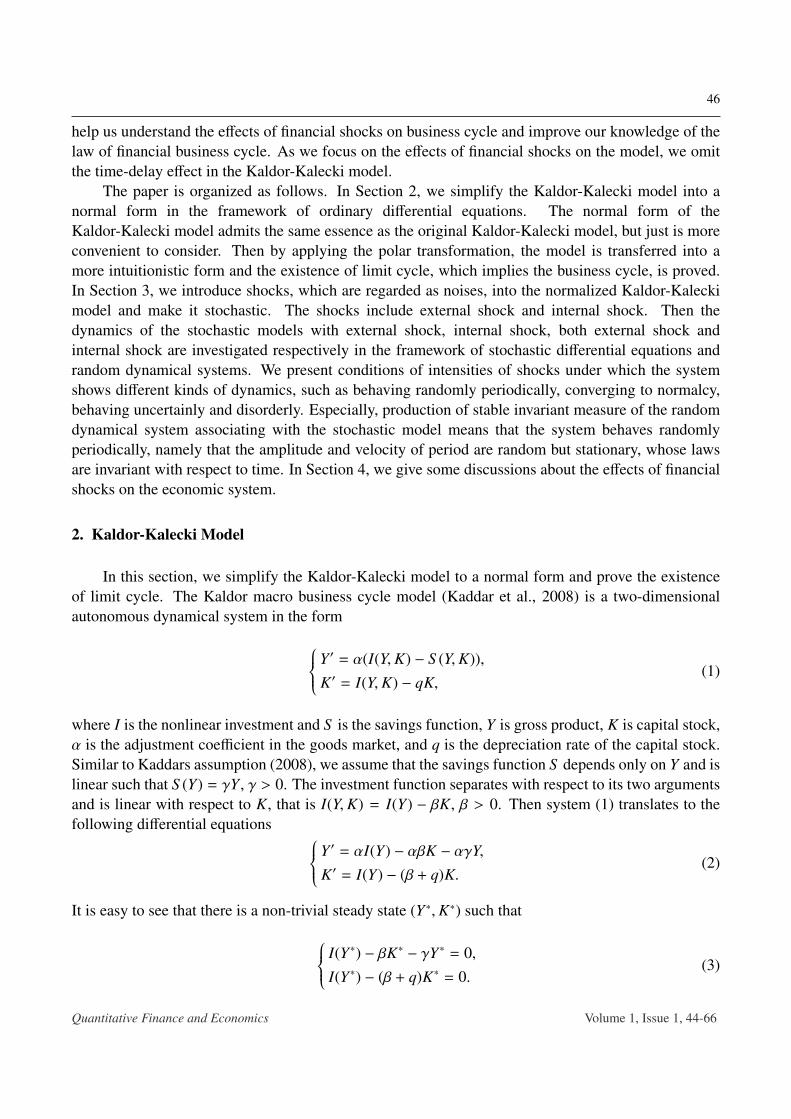
In Section 3, we have studied the dynamics of the business cycle model with external shock,internal shock, both external and internal shocks respectively in the framework of stochasticdifferential equations and random dynamical systems. The dynamics of the model can acquaint uswith the effects of shocks on the business cycle. In the case of external shock, if the intensity of theshock ε satisfies ε2 < 2λr, there exists an ergodic and stationary process r+(t) such that the original
amplitude r =
√−λrν
of the business cycle transfers to r+(t), which volatilities randomly. The original
velocity Θ′(t) = λcν−κλrν
of the business cycle transfers to Θ′(t) = λc + κr2+, which is also stationary. By
calculating the mean and mode of Θ′(t), we obtain two approximated estimations of period (26) and(28) in the case of external shock. Figure 1 shows the comparison among T , T1 and T2 as functions ofε. We can see that T1 and T2 are both larger than T for given an intensity of shock ε, namely that theperiod of business cycle may be enlarged due to the external shock. As the intensity of shockincreases, the period of business cycle increases as well. If the intensity of shock satisfies ε2 > 2λr,the amplitude of the business cycle converges to 0, which means that the economic system convergesto a normalcy (0, 0) (Actually, (0, 0) is not the real normalcy. One could understand this from (3), (4)and the context).
Figure 1. T , T1 and T2 as functions of ε in thecase of external shock, ε varies from 0.1 to 1,λr = λc = κ = 1, ν = −1.
In the case of internal shock, if the intensity of shock satisfies ε2 < 2λr
, the economic systemadmits the business cycle whose amplitude and velocity are the same as the original business cycle, soas the period.
Quantitative Finance and Economics Volume 1, Issue 1, 44-66
54
0.1 0.2 0.3 0.4 0.5 0.6 0.73
3.1
3.2
3.3
3.4
3.5
3.6
3.7
3.8
3.9
T
T1
T2
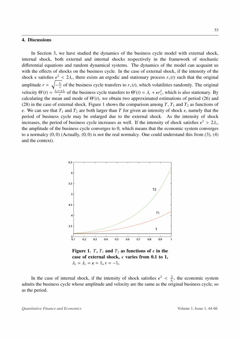
Figure 2. T , T1 and T2 as functions of ε2 in the case ofexternal and internal shocks, ε2 varies from 0.1 to 0.7,ε1 = 0.5, ρ = 0.5, λr = λc = κ = 1, ν = −1.
0.1 0.2 0.3 0.4 0.5 0.6 0.73
3.1
3.2
3.3
3.4
3.5
3.6
3.7
3.8
3.9
T
T1
T2
Figure 3. T , T1 and T2 as functions of ε1 in the case ofexternal and internal shocks, ε1 varies from 0.1 to 0.7,ε2 = 0.5, ρ = 0.5, λr = λc = κ = 1, ν = −1.
Quantitative Finance and Economics Volume 1, Issue 1, 44-66
55
0.1 0.2 0.3 0.4 0.5 0.6 0.73
3.1
3.2
3.3
3.4
3.5
3.6
3.7
3.8
3.9
T
T1
T2
Figure 4. T , T1 and T2 as functions of ε2 in the case ofexternal and internal shocks, ε2 varies from 0.1 to 0.7,ε1 = 0.5, ρ = −0.5, λr = λc = κ = 1, ν = −1.
0.1 0.2 0.3 0.4 0.5 0.6 0.73
3.1
3.2
3.3
3.4
3.5
3.6
3.7
3.8
3.9
T
T1
T2
Figure 5. T , T1 and T2 as functions of ε1 in the case ofexternal and internal shocks, ε1 varies from 0.1 to 0.7,ε2 = 0.5, ρ = −0.5, λr = λc = κ = 1, ν = −1.
If the intensity of shock satisfies ε2 > 2λr
, the business cycle exists in some probability less thanone. The system converges to a normalcy in residual probability. In summary, the system eitherbehaves periodically or converges to a normalcy. It is uncertain. In the case of external and internalshocks acting on the system, the effects of shocks on the business cycle are more complicated. If the
Quantitative Finance and Economics Volume 1, Issue 1, 44-66
56
intensities of shocks ε1 and ε2 satisfy 2λr > ε21 + 2ε1ε2ρλr + ε2
2λ2r , ε2
2ν2 < 3
2 , the economic systembehaves randomly periodically as the case of external shock, namely that the original amplitude andvelocity both transfer to stationary processes. We as well obtain two approximated periods given in(43) and (45). Figure 2 and Figure 3 show the comparison among T , T1 and T2 as functions of ε1 andε2 respectively under the assumption that external shock and internal shock are positively correlation,namely that ρ > 0. Figure 4 and Figure 5 show the same topic but under the assumption that externalshock and internal shock are negatively correlation, namely that ρ < 0. From the figures, we can seethat T1 is always larger than T regardless of the correlation of shocks. From Figure 2 and Figure 4,we can see that T2 may decrease as the intensity ε2 increases. In contrast, T1 increases as ε2 increases.Figure 3 and Figure 5 tell that both T1 and T2 may increase as the intensity ε1 increases. On the otherhand, from the increasing rate of T1, T2 and decreasing rate of T2 as functions of ε1 and ε2 in thefigures, we can see the sensitivity of the period of the business cycle on the intensities of shocks. Ifthe intensities of shocks satisfy 2λr < ε2
1 + 2ε1ε2ρλr + ε22λ
2r , ε2
2ν2 < 3
2 , the economic system convergesto the normalcy. However, if the intensities of shocks satisfy 2λr < ε2
1 + 2ε1ε2ρλr + ε22λ
2r , ε2
2ν2 > 3
2 ,the normalcy looses its stability and the system becomes disorder, which may implies the upcoming ofeconomic crisis.
A. The procedure of simplification of the system
To simplify the original system, denoting Λ = arg(λ), we can rewrite (11) asϕ′ =|λ| cos 2πΛϕ − |λ| sin 2πΛφ +
α
2λcI′′(0)ϕ2 +
α
6λ2cI′′′(0)ϕ3,
φ′ =|λ| sin 2πΛϕ + |λ| cos 2πΛφ −αq2λ2
cI′′(0)ϕ2 +
αq6λ3
cI′′′(0)ϕ3.
(A.1)
Then making the transformation of coordinates
ϕ =12
z +12
z, φ = −12
zi +12
zi, (A.2)
that isz = ϕ + φi, z = ϕ − φi, (A.3)
system (A.1) is translated into the following forms: z′ =λz + a20z2 + 2a11zz + a02z2+ b30z3 + 3b21z2z + 3b12zz2
Repeating the procedure above, denote h3(z, z) = h330z3 + h321z2z + h312zz2+ h303z3. Replacing z by
z + h3(z, z), then h3 must satisfy
− λ∂h3
∂zz + λ
∂h3
∂zz + λh3 + f30z3 + f21z2z + f12zz2
+ f03z3= 0. (A.12)
It is easy to solve that
h330 =f30
2λ, h321 = 0, h312 = −
f12
2λ, h303 = −
f03
4λ. (A.13)
Omitting the high order terms, system (A.10) is translated to
z′ = λz + f21z2z. (A.14)
Recalling that z = ϕ + φi, then we haveϕ′ = λrϕ − λcφ + (νϕ − κφ)(ϕ2 + φ2),φ′ = λcϕ + λrφ + (κϕ + νφ)(ϕ2 + φ2),
(A.15)
where ν = Re f21, κ = Im f21. From the arguments above, we can get
ν =αI′′′(0)16λ2
c−α2I′′2(0)8|λ|2λ2
c
(2q + λr +
(q + λr)2λr
λ2c
)(A.16)
and
κ = −α(q + λr)I′′′(0)
16λ3c
+α2I′′2(0)4|λ|2λc
(−
(q + λr)λr
λ2c
+(q + λr)2
2λ2c−
12
). (A.17)
Quantitative Finance and Economics Volume 1, Issue 1, 44-66
58
B. Proof of Proposition 3.1
The backward cocycle over θ := θ−1 corresponding to (18) is given by Φ(t, ω)r0 := Φ(−t, ω)r0. Itis generated by the stochastic differential equation
dr = −λrrdt − νr3dt + ε rdB(−t). (B.1)
First we restrict system Φ on R+. The Fokker-Plank equations of (18) and (B.1) are given respectivelyas
∂
∂tp(t, r) =
∂2
∂r2
(ε2
2r2 p(t, r)
)−∂
∂r((λrr + νr3)p(t, r)) (B.2)
and∂
∂tp(t, r) =
∂2
∂r2
(ε2
2r2 p(t, r)
)+∂
∂r((λrr + νr3) p(t, r)), (B.3)
whose time-homogeneous solutions can be solved by
p(r) = Cr(2λr−2ε2)/ε2exp
(ν
ε2 r2), p(r) = Cr−
2λrε2 exp
(−ν
ε2 r2). (B.4)
Then m(dr) = p(r)dr is the speed measure of Φ, which is an invariant measure of Markov semigroupPt associating with (18). m(dr) = p(r)dr is the speed measure of Φ, which is an invariant measure ofMarkov semigroup Pt associating with (B.1). Recall from Chapter 2 in Crauel and Gundlach (1999)that there is a bijection between the invariant probability measures of the semigroup and the Φ-invariantmeasures. If λr <
ε2
2 , m(R+) and m(R+) = ∞, which both can not be normalized. We conclude thatthere is no other Φ-invariant measures except δ0. To see the stability of invariant measure, we cancalculate the Lyapunov exponent. The linearization of Φ, DΦ(t, r) satisfies
2 , then m(R+) < ∞ and m(R+) = ∞. Moreover, for anyc > 0, m(R+/[0, c]) = ∞, which implies that Φ is forward complete (see Lemma 2.6 in Chapter 2in Crauel and Gundlach (1999)). Hence, there exists a random variable, denoted by r+, such thatδr+(ω) = lim
t→∞Φ(t, θtω)m/m(R+) is an ergodic Φ-invariant measure. Moreover,
r(ω) = 1/(− 2ν
∫ 0
−∞
exp(2λr s − ε2s + 2εB(s))ds) 1
2
(B.8)
Quantitative Finance and Economics Volume 1, Issue 1, 44-66
59
and
r(θtω) = exp(λrt −
ε2
2t + εB(t)
)/(− 2ν
∫ t
−∞
exp(2λr s − ε2s + 2εB(s))ds) 1
2
. (B.9)
The system occurs a D-bifurcation at λr = ε2
2 . To see the stability of δr+, we first give an estimation.
Denote R(r) = r2(t), where r is the solution of (18) with initial value r0 > 0. Then R satisfies
R(t) = exp(2λrt − ε2t + 2εB(t))/( 1r2
0
− 2ν∫ t
0exp(2λr s − ε2s + 2εB(s))ds
). (B.10)
Denote
Z(t) =1r2
0
− 2ν∫ t
0exp(2λr s − ε2s + 2εB(s))ds. (B.11)
It is easy to see that ∫ t
0R(s)ds = −
12ν
log Z(t) +12ν
log Z(0). (B.12)
By Doob’s inequality
P(
sup0≤s≤t|B(s)| ≥ ht
)≤ exp
(−
h2
2t), ∀h > 0, (B.13)
we have
P( 1r2
0
−2ν
2λr − ε2 exp((2λr − ε2 − 2εh)t) +
2ν2λr − ε2 exp(−2εht) ≤ Z(t)
≤1r2
0
−2ν
2λr − ε2 exp((2λr − ε2 + 2εh)t) +
2ν2λr − ε2 exp(2εht)
)≥ 1 − exp
(−
h2
2t).
(B.14)
It is easy to see that there exists T > 0, such that for t ≥ T ,
P(−
2ν2λr − ε2 exp((2λr − ε
2 − 2εh)t) ≤ Z(t) ≤ −2ν
2λr − ε2 exp((2λr − ε2 + 2εh)t)
)≥ 1 − exp
(−
h2
2t),
(B.15)
that is
P(−
12ν
log(−
2ν2λr − ε2
)−
12ν
(2λr − ε2 − 2εh)t ≤ −
12ν
log Z(t)
≤ −12ν
log(−
2νλr − ε2
)−
12ν
(2λr − ε2 + 2εh)t
)≥ 1 − exp
(−
h2
2t),
(B.16)
which implies
−12ν
(2λr − ε2 − 2εh) ≤ −
12ν
limt→∞
1t
log Z(t) ≤ −12ν
(2λr − ε2 + 2εh). (B.17)
Since h is arbitrary, we have
limt→∞
1t
∫ t
0R(s)ds = −
12ν
limt→∞
1t
log Z(t) =12ν
(ε2 − 2λr) (B.18)
Quantitative Finance and Economics Volume 1, Issue 1, 44-66
60
almost surely. Applying this result, the Lyapunov exponent of λΦ(δr+) satisfies
λΦ(δr+) =lim
t→∞
1t
log DΦ(t, r+)
=limt→∞
1t
∫ t
0
(λr −
ε2
2+ 2νr2
+(θsω))ds
=λr −ε2
2+ 2νlim
t→∞
1t
∫ t
0r2
+(θsω)ds
=λr −ε2
2− 2λr + ε2
= − λr +ε2
2< 0,
(B.19)
which implies that δr+is stable. At the same time, δ0 becomes unstable. If ε2
2 < λr < ε2, the maximum
of p is located at r = 0. If λr > ε2, the maximum of p is located at r∗, where
r∗ =
√ε2 − λr
ν. (B.20)
Therefore the system occurs a P-bifurcation at λr = ε2. Restricting Φ on R− and following thearguments above, similarly, we can obtain another ergodic Φ-invariant measure, denoted by δr− , whichis also stable. Hence, we conclude that the system occurs a pitchfork bifurcation at λr = ε2
2 .
C. Proof of Proposition 3.2
Denote R(t) = r2(t). Then by Ito’s formula, we have
Denote Y(t) = log R(t)λr+νR(t) = log R(t) − log(λr + νR(r)). Again by Ito’s formula, we have
dY = (2λr − ε2λ2
r − 3λrε2νR)dt + 2ελrdB(t), (C.2)
or
logR(t)
λr + νR(t)= log
R0
λr + νR0+ (2λr − ε
2λ2r )t − 3λrε
2ν
∫ t
0R(s)ds + 2ελrB(t), (C.3)
where we have assumed that B(0) = 0. By Doob’s inequality (C.4), we have
P(
logR(t)
λr + νR(t)≥ log
R0
λr + νR0+ (2λr − ε
2λ2r )t − 2ελrht
)≥ 1 − exp
(−
h2
2t), (C.4)
where R0 > 0 is the initial condition. Since ε2λr < 2, namely 2λr − ε2λ2
r > 0 and h > 0 is arbitrary, wehave
limt→∞
logR(t)
λr + νR(t)≥ log
R0
λr + νR0+ lim
t→∞(2λr − ε
2λ2r − 2ελrh)t = ∞ (C.5)
almost surely, which is possible only if limt→∞
R(t) = −λrν
almost surely.
Quantitative Finance and Economics Volume 1, Issue 1, 44-66
61
For a function f ∈ C2(R+), by Ito’s formula, we have
d f (R) = f ′(R)dR +12
f ′′(R)d〈R〉
= f ′(R)R(2 + λrε2 + ε2νR)(λr + νR)dt + 2ε f ′(R)R(λr + νR)dB(t)
+ 2ε2 f ′′(R)R2(λr + νR)2dt.
(C.6)
Letting f satisfy
f ′(R)R(2 + λrε2 + ε2νR)(λr + νR) + 2ε2 f ′′(R)R2(λr + νR)2 = 0, (C.7)
we can solve that
f (R) =
∫ R
0x−
(1
ε2λr+ 1
2
)(−λr
ν− x
) 1ε2λr dx. (C.8)
For 0 < R0 < −λrν
,
limt→∞E[ f (R(t))] = f
(−λr
ν
)P(R(t)→ −
λr
νas t → ∞
). (C.9)
On the other hand, since f (R(t)) is a martingale, we have
f (R0) = f(−λr
ν
)P(R(t)→ −
λr
νas t → ∞
), (C.10)
namely that
P(R(t)→ −
λr
νas t → ∞
)= f (R0)/ f
(−λr
ν
), (C.11)
which implies that
P(R(t)→ 0 as t → ∞) = 1 − f (R0)/ f(−λr
ν
). (C.12)
D. Proof of Proposition 3.3
Making the transformation B1(t) = B1(t),
B2(t) = ρB1(t) +√
1 − ρ2B2(t),(D.1)
it is easy to check that 〈B1, B2〉 = 0, namely that B1 and B2 are mutually independent Brownian motions.First equation in system (36) can be rewritten as
which is equivalent in law to the following equation
dx =
((λr −
α
2
)x + (ν − β)x3 −
32γx5
)dt +
√αx2 + βx4 + γx6 dB(t), (D.3)
whereα = ε2
1 + 2ε1ε2ρλr + ε22λ
2r , β = 2ε1ε2ρν + 2ε2
2λrν, γ = ε22ν
2, (D.4)
Quantitative Finance and Economics Volume 1, Issue 1, 44-66
62
associating with random dynamical system Φ represented by
Ψ(t, ω)x0 =x0 +
∫ t
0
((λr −
α
2
)Ψ(s, ω)x0 + (ν − β)Ψ3(s, ω)x0 −
32γΨ5(s, ω)x0
)ds
+
∫ t
0
√αΨ2(s, ω)x0 + βΨ4(s, ω)x0 + γΨ6(s, ω)x0 dB(s)
(D.5)
with initial value x0 > 0. The backward cocycle over θ corresponding to (D.5) is given by Ψ(t, ω)x0 :=Ψ(−t, ω)x0, which is generated by the stochastic differential equation
dx =
(−
(λr −
α
2
)x − (ν − β)x3 +
32γx5
)dt +
√αx2 + βx4 + γx6 dB(−t). (D.6)
The Fokker-Plank equations of (D.3) and (D.6) can be written as
∂
∂tp(t, x) =
∂2
∂x2
(12
(αx2 + βx4 + γx6)p(t, x))−∂
∂x((λr x + νx3)p(t, x)) (D.7)
and∂
∂tp(t, x) =
∂2
∂x2
(12
(αx2 + βx4 + γx6) p(t, x))
+∂
∂x((λr x + νx3) p(t, x)), (D.8)
whose time-homogeneous solutions can be solved by
p(x) =2√
αx2 + βx4 + γx6exp
(2∫ x
c
(λr −α2 )y + (ν − β)y3 − 3
2γy5
αy2 + βy4 + γy6 dy)
(D.9)
and
p(x) =2√
αx2 + βx4 + γx6exp
(2∫ x
c
−(λr −α2 )y − (ν − β)y3 + 3
2γy5
αy2 + βy4 + γy6 dy). (D.10)
m(dx) = p(x)dx is an invariant measure of the Markov semigroup associating with (D.3) and m(dx) =
p(x)dx is an invariant measure of Markov semigroup associating with (D.6). If x > 0 is small enough,it is easy to see that
exp(2∫ x
c
(λr −α2 )y + (ν − β)y3 − 3
2y5
αy2 + βy4 + γy6 dy)≈ exp
(2λr − α
α
∫ x
c
1y
dy)
= Cx2λr−αα (D.11)
and
exp(2∫ x
c
−(λr −α2 )y − (ν − β)y3 + 3
2y5
αy2 + βy4 + γy6 dy)≈ exp
(α − 2λr
α
∫ x
c
1y
dy)
= Cxα−2λrα , (D.12)
which implies that for x > 0 is small enough, p(x) ≈ Cx2λr−2α
α and p(x) ≈ Cx−2λrα . If x > 0 is large
enough, it is easy to see that
exp(2∫ x
c
(λr −α2 )y + (ν − β)y3 − 3
2y5
αy2 + βy4 + γy6 dy)≈ exp
(−
3γ
∫ x
c
1y
dy)
= Cx−3γ (D.13)
Quantitative Finance and Economics Volume 1, Issue 1, 44-66
63
and
exp(2∫ x
c
−(λr −α2 )y − (ν − β)y3 + 3
2y5
αy2 + βy4 + γy6 dy)≈ exp
(3γ
∫ x
c
1y
dy)
= Cx3γ , (D.14)
which implies that for x > 0 large enough, p(x) ≈ Cx−3− 3γ and p(x) ≈ Cx−3+ 3
γ . If λr >α2 , m(R+) < ∞
and m(R+) = ∞. If γ < 32 , then for any c > 0, m(R+/[0, c]) = ∞. From Lemma 2.6 in Chapter 2 in
Crauel and Gundlach (1999), Ψ is forward complete. Hence, there exists a random variable x+ suchthat δx+
= limt→∞
Ψ(t, θtω)m/m(R+) is an ergodic invariant measure. If λr <α2 , γ > 3
2 , then m(R+) < ∞and m(R+) = ∞. But for any c > 0, m(R+/[0, c]) < ∞, which implies that Ψ is not backward complete.Hence, there is no other invariant measures except δ0. We conclude that system occurs a D-bifurcationat λr = α
2 , γ = 32 . Now let γ < 3
2 . If α2 < λr < α, the maximum of p is located at 0. If λr > α, the
maximum of p is located at x∗, where x∗ satisfies
3γx4∗ + (2β − ν)x2
∗ + α − λr = 0, (D.15)
which can be solved as
x∗ =
√(ν − 2β) +
√(2β − ν)2 − 12γ(α − λr)
6γ. (D.16)
We conclude that system occurs a P-bifurcation at λr = α. The aforesaid results for Ψ hold for Φ
as well, namely that Φ occurs D-bifurcation at λr = α2 , γ = 3
2 . We denote the generated non-trivialinvariant measure as δr+
. Φ occurs P-bifurcation at λr = α, the maximum of the probability densityfunction is located at r∗ = x∗. To see the stabilities of the invariant measures, we calculate the Lyapunovexponents. The linearization of Φ, DΦ(t, r) satisfies
Quantitative Finance and Economics Volume 1, Issue 1, 44-66
64
Taking logarithm in (D.2) and dividing by t, we have
1t
log r(t) =1t
log r0 + λr + ν1t
∫ t
0r2(s)ds −
12t
∫ t
0(ε1 + ρε2(λr + νr2(s)))2ds
−12
(1 − ρ2)ε22
1t
∫ t
0(λr + νr2(s))2ds +
1t
∫ t
0(ε1 + ρε2(λr + νr2(s)))dB1(s)
+√
1 − ρ2ε21t
∫ t
0(λr + νr2(s))dB2(s)
=1t
log r0 + λr −α
2+
(ν −
β
2
)1t
∫ t
0r2(s)ds −
γ
21t
∫ t
0r4(s)ds
+ (ε1 + ρε2λr)1t
B1(t) + ρε2ν1t
∫ t
0r2(s)dB1(s)
+√
1 − ρ2ε2λr1t
B2(t) +√
1 − ρ2ε2ν1t
∫ t
0r2(s)dB2(s).
(D.19)
By Doob’s inequality, we know that limt→∞
1t B1(t) = lim
t→∞1t B2(t) = 0 almost surely. Since r+(θtω) is ergodic
and stationary process, letting r(t) = r+(θtω) in (D.19) and t → ∞, we have
limt→∞
((ν −
β
2
)1t
∫ t
0r2
+(θsω)ds −γ
2t
∫ t
0r4
+(θsω)ds
+ ρε2ν1t
∫ t
0r2
+(θsω)dB1(s) +√
1 − ρ2ε2ν1t
∫ t
0r2
+(θsω)dB2(s))
=α
2− λr
(D.20)
almost surely. If λr >α2 , associating with (D.18) and (D.20), we have
limt→∞
1t
log DΦ(t, r+)V = −2(λr −
α
2
)− 3γlim
t→∞
1t
∫ t
0r4
+(θsω)ds < 0 (D.21)
almost surely, which implies the stability of the invariant measure δr+. At the same time, it is easy to
check thatlimt→∞
1t
log DΦ(t, 0)V = λr −α
2> 0 (D.22)
almost surely, which implies that δ0 is unstable. If λr < α2 , then δ0 is stable. On the other hand,
restricting Φ on R− and following the arguments above, we obtain another ergodic invariant measuresupporting on R−, which is also stable if λr >
α2 , γ < 3
2 . We conclude that if γ < 32 , system Φ occurs a
pitchfork bifurcation at λr = α2 .
Acknowledgments
We are grateful to the fund project - the Key Subject Funds of Guangzhou Financial Research(No.16GFR02B09) providing us with funding support.
Conflict of Interest
The author declares no conflict of interest in this paper.
Quantitative Finance and Economics Volume 1, Issue 1, 44-66
65
References
Alpanda S, Aysun U (2014) International transmission of financial shocks in an estimated DSGEmodel. J Int Money Financ 47: 21-55.
Arnold L (1998) Random Dynamical Systems. Springer.
Bashkirtseva I, Ryashko L, Sysolyatina A (2016) Analysis of stochastic effects in Kaldor-typebusiness cycle discrete model. Commun Nonlinear Sci Numer Simulat 36: 446-456.
Chang W, Smyth DJ (1972) The existence and persistence of cycles in a nonlinear model: Kaldor’s1940 model reexamined. Rev Econ Stud 38: 37-44.
Christiano L, Motto R, Rostagno M (2007) Financial factors in business cycles. NorthwesternUniversity Working Paper.
Claessens S, Kose MA, Terrones ME (2012) How do business and financial cycles interact? J IntEcon 87: 178-190.
Crauel H, Gundlach M (1999) Stochastic Dynamics. Springer.
De Cesare L, Sportelli M (2012) Fiscal policy lags and income adjustment processes. Chaos, SolitonsFractals 45: 433-438.
Grasman J, Wentzel JJ (1994) Co-Existence of a limit cycle and an equilibrium in Kaldor’s businesscycle model and it’s consequences. J Econ Behav Organ 24: 369-377.
Huang Z, Liu Z (2016) Random traveling wave and bifurcations of asymptotic behaviors in thestochastic KPP equation driven by dual noises. J Differ Equ 261: 1317-1356.
Iacoviello M (2015) Financial business cycles. Rev Econ Dyn 18: 140-163.
Jerman U, Quadrini V (2012) Macroeconomic effects of financial shocks. Am Econ Rev 102: 238-271.
Kaddar A, Talibi Alaoui H (2008) Hopf bifurcation analysis in a delayed Kaldor-Kalecki model ofbusiness cycle. Nonlinear Anal: Model Control 13: 439-449.
Kaddar A, Talibi Alaoui H (2009) Local Hopf Bifurcation and Stability of Limit Cycle in a DelayedKaldor-Kalecki Model. Nonlinear Anal: Model Control 14: 333-343.
Kaldor N (1940) A model of the trade cycle. Econ J 50: 78-92.
Kalecki M (1935) A macrodynamic theory of business cycle. Econom 3: 327-344.
Kalecki M (1937) A theory of the business cycle. Rev Stud 4: 77-97.
Kamber G, Thoenissen C (2013) Financial exposure and the international transmission of financialshocks. J Money, Credit Bank 45: 127-158
Krawiec A, Szydłowski M (1999) The Kaldor-Kalecki business cycle model. Ann Oper Res 89: 89-100.
Quantitative Finance and Economics Volume 1, Issue 1, 44-66
66
Kollmann R (2013) Global banks, financial shocks, and international business cycles: Evidence froman estimated model. J Money, Credit Bank 45: 159-195.
Kynes JM (1936) The General Theory of Employment, Interest Money. Macmillan CambridgeUniversity Press.
Luca D, Lombardo G (2009) Financial frictions, financial integration and the internationalpropagation of shocks. Econ Policy 27: 321-359.
Liao X, Li C, Zhou S (2005) Hopf bifurcation and chaos in macroeconomic models with policy lag.Chaos, Solitons Fractals 25: 91-108.
Mimir Y (2016) Financial intermediaries, credit shocks and business cycles. Oxf Bul Econ Stat 78:42-74.
Mircea G, Neamtu M, Opris D (2011) The Kaldor-Kalecki stochastic model of business cycle.Nonlinear Anal: Model Control 16: 191-205.
Øksendal B (2000) Stochastic Differential Equations: An Introduction with Applications. Springer.
Øksendal B, Våge G, Zhao H (2001) Two properties of stochastic KPP equations: ergodicity andpathwise property. Nonlinearity 14: 639-662.
Szydłwski M, Krawiec A, Toboła J (2001) Nonlinear oscillations in business cycle model with timelags. Chaos, Solitons Fractals 12: 505-517.
Szydłwski M, Krawiec A (2001) The Kaldor-Kalecki Model of business cycle as a two-dimensionaldynamical system. J Nonlinear Math Phys 8: 266-271.
Szydłwski M, Krawiec A (2005) The stability problem in the Kaldor-Kalecki business cycle model.Chaos, Solitons Fractals 25: 299-305.
Varian HR (1979) Catastrophe theory and the business cycle. Econ Inq 17: 14-28.
Wang L, Wu X (2009) Bifurcation analysis of a Kaldor-Kalecki model of business cycle with timedelay. Electron J Qual Theory Differ Eq 27: 1-20.
Wu X (2012) Zero-Hopf bifurcation analysis of a Kaldor-Kalecki model of business cycle with delay.Nonlinear Anal: Real World Appl 13: 736-754.
Zhang C, Wei J (2004) Stability and bifurcation analysis in a kind of business cycle model with delay.Chaos, Solitons Fractals 22: 883-896.