60
Modeling Decision Process Chapter 5
| Date post: | 19-Dec-2015 |
| Category: |
Documents |
| View: | 214 times |
| Download: | 1 times |

Modeling Decision Process
Chapter 5

The What's & Whys of Modeling What is a model?
A replica of a real system or object. An abstraction of reality
Model formats: Physical Graphical Verbal Mathematical

The What's & Whys of Modeling Why do we use models:
Understanding through simplification. Demonstrating and evaluating cause and
effect relationships. Experimenting with decision alternatives
on the real system is infeasible, too expensive, too dangerous, or just plain impossible.
Need for time compression for analysis of a system or prediction of future values.
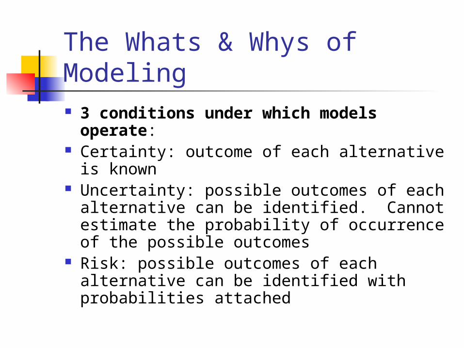
The Whats & Whys of Modeling 3 conditions under which models
operate: Certainty: outcome of each alternative is
known Uncertainty: possible outcomes of each
alternative can be identified. Cannot estimate the probability of occurrence of the possible outcomes
Risk: possible outcomes of each alternative can be identified with probabilities attached
Basic Model Types
A survey of Models
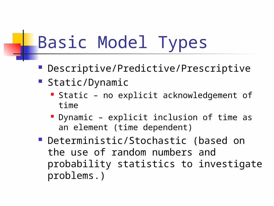
Basic Model Types Descriptive/Predictive/Prescriptive Static/Dynamic
Static – no explicit acknowledgement of time
Dynamic – explicit inclusion of time as an element (time dependent)
Deterministic/Stochastic (based on the use of random numbers and probability statistics to investigate problems.)

Decision Model Classification Deterministic – optimization, linear
programming, financial planning, production planning, convex programming.
Probabilistic – queuing theory, linear regression, logic analysis, path analysis, time series.
Simulation – production modeling, transportation and logistics analysis, econometrics.

Modeling Steps Define & analyze the problem Select and/or construct the model
Variables: controllable Parameters: not controllable Objectives: singular or multiple Constraints: limits on possible solution
The model establishes relationships among variables, parameters, objectives, and constraints

Modeling Steps Validate the model: does the model
accurately represent the real system? Compare model output with historical or
real world data Have model evaluated by experts Have model evaluated by decision-makers Compare model output with expectations
based on experience & expertise

Modeling Steps Acquire input data
Input data must be accurate & timely. Use data to design modeling experiments
Solve the model / develop the solution Test the model solution
Is it realistic ? Is it valid? Sensitivity analysis of modeling
results Implementation of modeling results

Modeling & Decision-Making Strategies
Optimization Economic Optimization Utility Optimization
Satisficing “Good enough” solution Application of Heuristics
Elimination-by-Aspects Stepwise application of decision criteria

Modeling & Decision-Making Strategies
Incrementalism Decision are based on past decision
outcomes Mixed Scanning
Elimination of alternatives through increasing amounts of information gathering

Influence Diagrams and Decision Trees
Influence Diagram A simple graphical representation of a
model Decision Tree
Complement influence diagram Modeling of choices and uncertainties

Components of Influence Diagrams and Decision Trees
DecisionsDecisions UncertaintiesUncertainties Final Outcomes
DecisionDecision
Alternative AAlternative A
Alternative B
Alternative CAlternative C
Alternative DAlternative D
Outcome AOutcome A
Outcome BOutcome B
Outcome COutcome C
Outcome DOutcome D

Uncertainty Model with Outcomes
Sales VolumeSales Volume
Low 0.30Low 0.30
Medium 0.50Medium 0.50
High 0.20High 0.20

Simple Decision Tree
Enter Contest
Do Not Enter Contest
Win ContestWin Contest
Lose Contest
Win large return on wager
Lose wager
Lose/Gain nothing

Basic Risky Decision
Decision
Uncertainty
ObjectiveObjective
Buy Stock
Do Not Buy Stock
Price goes upPrice goes up
Price goes down
Gain
Loss
Lose/Gain nothing

Decision Tree for Odds Forecasting Method
Bet on Vikes
Bet Against VikesBet Against Vikes
Vikes Win
Vikes Win
Vikes Lose
Vikes Lose
$X
-$X
-$Y
$Y

Decision Tree for Comparison Forecasting Method
Uncertainty Game
Reference GameReference Game
Win
(P)
Lose
(1 – P)
European Vacation
-$100
European Vacation
-$100

A Variety of Models Decision Tables Game Theory Mathematical & Linear
Programming Simulation Forecasting Analytic Hierarchy Process

Decision Tables Decision Alternatives
Controllable State of Nature
Not controllable Uncertainty or Risk
Payoffs Product of Decision Alternative and
states of Nature

Decision Tables Decision Goal: what new store to
open
State of Nature Alternative recision recovery economic boom
Stereo Eqpmt 10,000 30,000 60,000Book Store 30,000 45,000 20,000Food Store 55,000 30,000 10,000

Decision Tables / Uncertainty
State of Nature
Alternative recision recovery economic boom
Stereo Eqpmt 10,000 30,000 60,000
Book Store 30,000 45,000 20,000
Food Store 55,000 30,000 10,000
• Optimistic Criterion: Stereo Equipment
•Highest payoff in table
• Pessimistic criterion: Book Store
•Take best of the worst payoffs of each alternatives
• Equal likelihood Criterion: Stereo Eqpmt.
•Highest average payoff per alternative
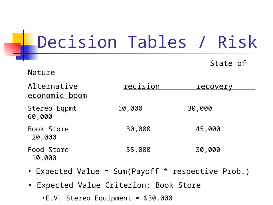
Decision Tables / Risk State of Nature
Alternative recision recovery economic boom
Stereo Eqpmt 10,000 30,000 60,000
Book Store 30,000 45,000 20,000
Food Store 55,000 30,000 10,000
• Expected Value = Sum(Payoff * respective Prob.)
• Expected Value Criterion: Book Store
•E.V. Stereo Equipment = $30,000
•E.V. Book Store = $35,500
•E.V. Discount Foods = $33,500

Game Theory Two (or more) players. Players act in self-interest only. Players have full information on
each other’s strategies or payoffs. Zero-Sum Game: one player’s
profit is the other player’s loss Non-Zero-Sum Game: both players
may win or lose simultaneously.

Mathematical Programming Modeling using mathematical
equations Usually requires solving for variables
and for simultaneous equations Linear Programming
Standard, programmable solution techniques
Non-Linear Programming Usually requires mathematical expertise

Linear Programming Furniture Makers Production Mix
Problem: Which production combination yields the
highest profit?
Tables Chairs Hours Avail.Carpentry 4 hrs 3 hrs 240 hours Painting 2 hrs 1 hr 100 hoursProfit/Unit $7 $5

Linear Programming Objective Function Max 7 T + 5 C
Constraints: Carpentry: 4 T + 3 C <= 240 Painting: 2 T + 1 C <=100 Non-negativity T,C >=0 Optimal Solution: Tables = 30 Chairs = 40 Revenue = 410

Simulation “The use of a model to represent the
critical characteristics of a system and to observe the system’s operations over time.”
Most common dynamic process modeling type.
Given heavy use of computers, simulation now very much resembles programming!
Monte Carlo Simulation Simulation of randomness into a
system, using Random Number Generator Cumulative Probability Distribution

Monte Carlo Simulation The Bakery Problem: how many
chocolate donuts to bake each day? Gather sales data for 100 days Sales Frequency Probability
30 20 days 20 %
31 35 days 35 %32 25 days 25 %33 15 days 15 %34 5 days 5 %
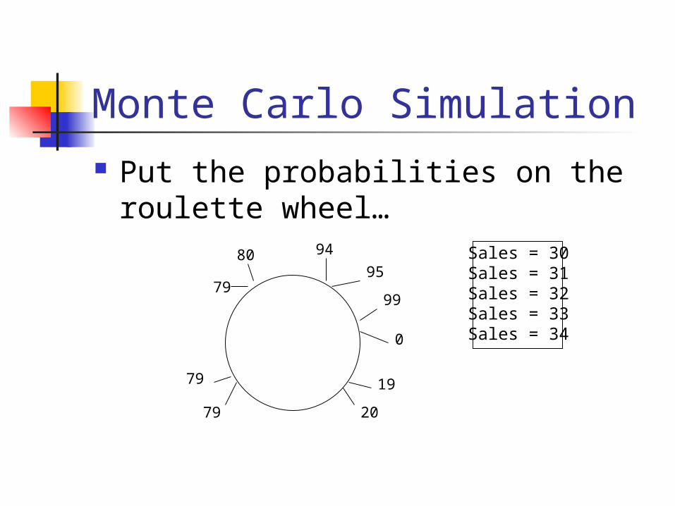
Monte Carlo Simulation Put the probabilities on the
roulette wheel…
79
80 94
95
99
0
79
20
19
79
Sales = 30Sales = 31Sales = 32Sales = 33Sales = 34

Monte Carlo Simulation …and start simulating
Generate a random number: 00-99 Find this number on the roulette-
wheel. Find the matching sales-levels Random Number Sales Level
35 31 donuts 82 33 donuts 01 30 donuts

Forecasting The prediction of future values,
based on past experience. Prediction based on personal
expertise. Prediction based on a mathematical
model.
Mathematical Forecasting A variety of techniques
Linear & Nonlinear regression Time Series / Box –Jenkins Technique Etc
These techniques differ in predictive quality, applicability, and ease of use

Forecasting - Regression The fitting of a line to a cloud of
observation-points, based on minimizing the distance between the line and the set of points
Dependentvariable
Independent variable

Forecasting - Regression Standard linear regression function:
Y = a + bX Y = dependent(forecast) variable X = independent variable a = intercept b = slope
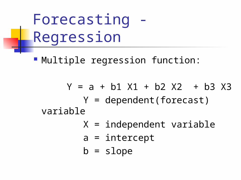
Forecasting - Regression Multiple regression function:
Y = a + b1 X1 + b2 X2 + b3 X3 Y = dependent(forecast) variable X = independent variable a = intercept b = slope

Analytic Hierarchy Process
Method to solve Multiple-criteria decision-making
Specifies: Decision goal Decision Criteria Decision Alternatives
Real world decision problems multiple, diverse criteria qualitative as well as quantitative
information

Analytic Hierarchy Process
Comparing apples and oranges?Spend on defense or agriculture?Open the refrigerator - apple or orange?

Analytic Hierarchy Process
Goal
Criterion
Criterion Criterion
Alt. 1 Alt. 1 Alt. 1Alt. 2 Alt. 2 Alt. 2
Alt. 3 Alt. 3Alt. 3
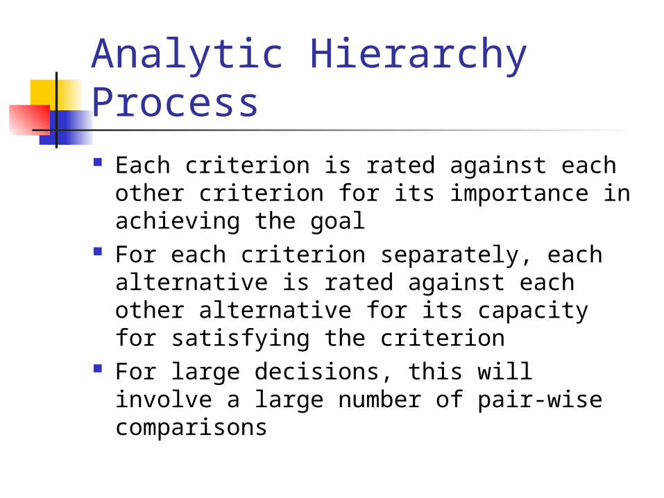
Analytic Hierarchy Process Each criterion is rated against each
other criterion for its importance in achieving the goal
For each criterion separately, each alternative is rated against each other alternative for its capacity for satisfying the criterion
For large decisions, this will involve a large number of pair-wise comparisons

Analytic Hierarchy Process AHP computer programs determine
the consistency of the pair-wise comparisons. Sometimes, the comparison-phase
will need to be repeated If consistent, the AHP program will
provide a rank-order of the alternatives
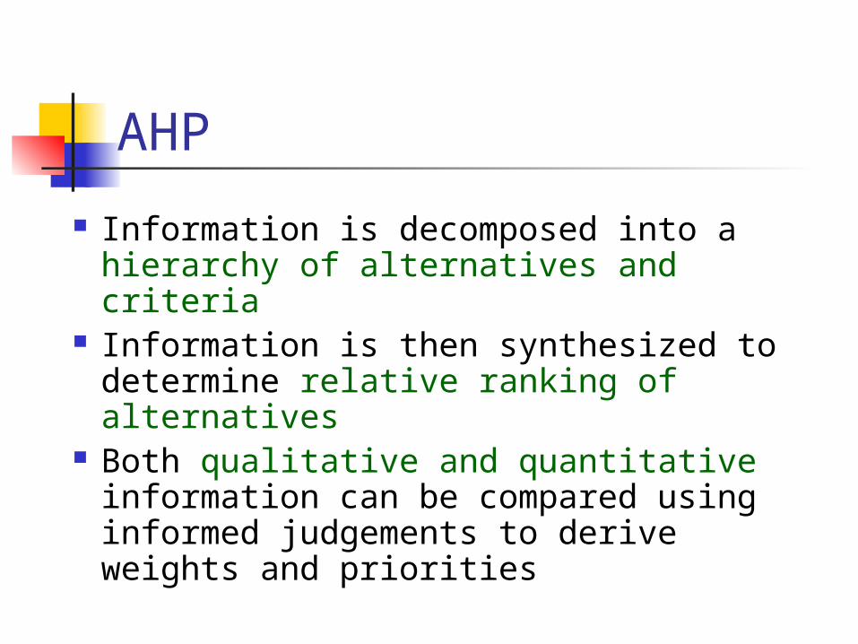
AHP
Information is decomposed into a hierarchy of alternatives and criteria
Information is then synthesized to determine relative ranking of alternatives
Both qualitative and quantitative information can be compared using informed judgements to derive weights and priorities

Example: Car Selection
Objective Selecting a car
Criteria Style, Reliability, Fuel-economy
Cost? Alternatives
Civic Coupe, Saturn Coupe, Ford Escort, Mazda Miata
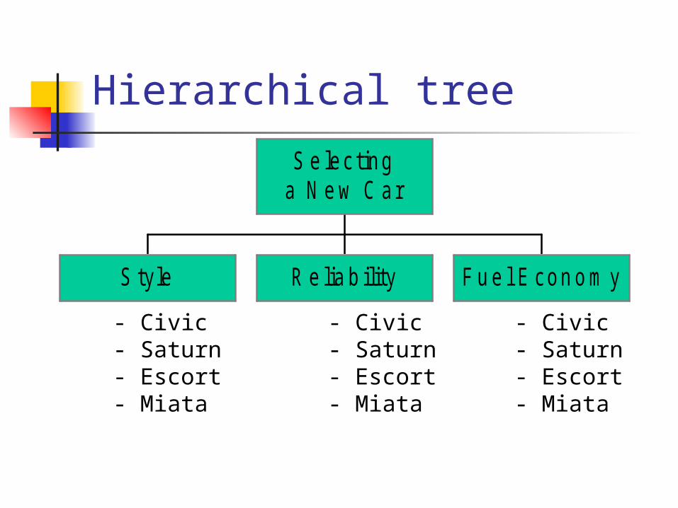
Hierarchical tree
S tyle R e lia b ility F u e l E con o m y
S e lec tinga N e w C ar
- Civic- Saturn- Escort- Miata
- Civic- Saturn- Escort- Miata
- Civic- Saturn- Escort- Miata

Ranking of criteria
Weights? AHP
pair-wise relative importance [1:Equal, 3:Moderate, 5:Strong, 7:Very strong,
9:Extreme]
Style Reliability Fuel Economy
Style
Reliability
Fuel Economy
1/1 1/2 3/1
2/1 1/1 4/1
1/3 1/4 1/1
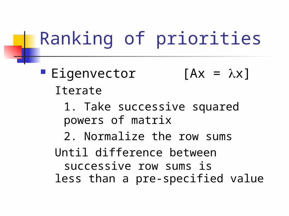
Ranking of priorities
Eigenvector [Ax = x]Iterate
1. Take successive squared powers of matrix2. Normalize the row sums
Until difference between successive row sums is
less than a pre-specified value

1 0.5 32 1 40.333 0.25 1.0
3.0 1.75 8.05.3332 3.0 14.01.1666 0.6667 3.0
squared
Row sums 12.75 22.3332 4.8333
39.9165
NormalizedRow sums 0.3194 0.5595 0.1211
1.0
• New iteration gives normalized row sum 0.3196 0.5584 0.1220
• Difference is: - 0.3194 0.5595 0.1211
0.3196 0.5584 0.1220
= - 0.0002 0.0011 - 0.0009

Preference Style .3196 Reliability .5584 Fuel Economy .1220
S tyle.3 196
R e lia b ility.5 584
F u e l E con o m y.1 220
S e lec tinga N e w C ar
1 .0

Ranking alternatives
Style
Civic
Saturn
Escort
1/1 1/4 4/1 1/6
4/1 1/1 4/1 1/4
1/4 1/4 1/1 1/5
Miata 6/1 4/1 5/1 1/1
Civic Saturn Escort Miata
Miata
Reliability
Civic
Saturn
Escort
1/1 2/1 5/1 1/1
1/2 1/1 3/1 2/1
1/5 1/3 1/1 1/4
Miata 1/1 1/2 4/1 1/1
Civic Saturn Escort Miata
.1160
.2470
.0600
.5770
Eigenvector
.3790
.2900
.0740
.2570

Fuel Economy(quantitative information)
Civic
Saturn
Escort
MiataMiata
34
27
24
28 113
Miles/gallon Normalized
.3010
.2390
.2120
.2480 1.0

S tyle.3 196
R e lia b ility.5 584
F u e l E con o m y.1 220
S e lec tinga N e w C ar
1 .0
- Civic .1160- Saturn .2470- Escort .0600- Miata .5770
- Civic .3790 - Saturn .2900- Escort .0740- Miata .2570
- Civic .3010- Saturn .2390- Escort .2120- Miata .2480

Ranking of alternatives
Style Reliability Fuel Economy
Civic
EscortMiataMiata
Saturn
.1160 .3790 .3010
.2470 .2900 .2390
.0600 .0740 .2120
.5770 .2570 .2480
* .3196
.5584
.1220
= .3060
.2720
.0940
.3280

Handling Costs
Dangers of including Cost as another criterion political, emotional responses?
Separate Benefits and Costs hierarchical trees
Costs vs. Benefits evaluation Alternative with best benefits/costs ratio

Cost vs. Benefits
MIATA $18K .333.9840
CIVIC $12K .222 1.3771
SATURN $15K .2778.9791
ESCORT $9K .1667.5639
CostNormalized Cost
Cost/Benefits Ratio

Complex decisions•Many levels of criteria and sub-criteria

Application areas strategic planning resource allocation source selection, program selection business policy etc., etc., etc..
AHP software (ExpertChoice) computations sensitivity analysis graphs, tables
Group AHP

Model Management Model Base Management System Basic Features:
Tracking a large variety of models, model-types, model-versions, purposes, etc.
Provide access to model & model descriptions.
Provide for new models and model updates to be placed in Model Base.

Model Management Model Base Management System Advanced Features Suggest appropriate models to
decision maker. Relate models to required data
from DSS database Allow decision maker to customize
models or build new models


