Contents: Textbook: References: Topic 18 Modeling of Elasto-Plastic and Creep Response Part II • Strain formulas to model creep strains • Assumption of creep strain hardening for varying stress situations • Creep in multiaxial stress conditions, use of effective stress and effective creep strain • Explicit and implicit integration of stress • Selection of size of time step in stress integration • Thermo-plasticity and creep, temperature-dependency of material constants • Example analysis: Numerical uniaxial creep results • Example analysis: Collapse analysis of a column with offset load • Example analysis: Analysis of cylinder subjected to heat treatment Section 6.4.2 The computations in thermo-elasto-plastic-creep analysis are described in Snyder, M. D., and K. J. Bathe, "A Solution Procedure for Thermo-Elas- tic-Plastic and Creep Problems," Nuclear Engineering and Design, 64, 49-80, 1981. Cesar, F., and K. J. Bathe, "A Finite Element Analysis of Quenching Processes," in Numerical Methods jor Non-Linear Problems, (Taylor, C., et al. eds.), Pineridge Press, 1984.
Transcript
Contents:
Textbook:
References:
Topic 18
Modeling ofElasto-Plastic andCreepResponse Part II
• Strain formulas to model creep strains
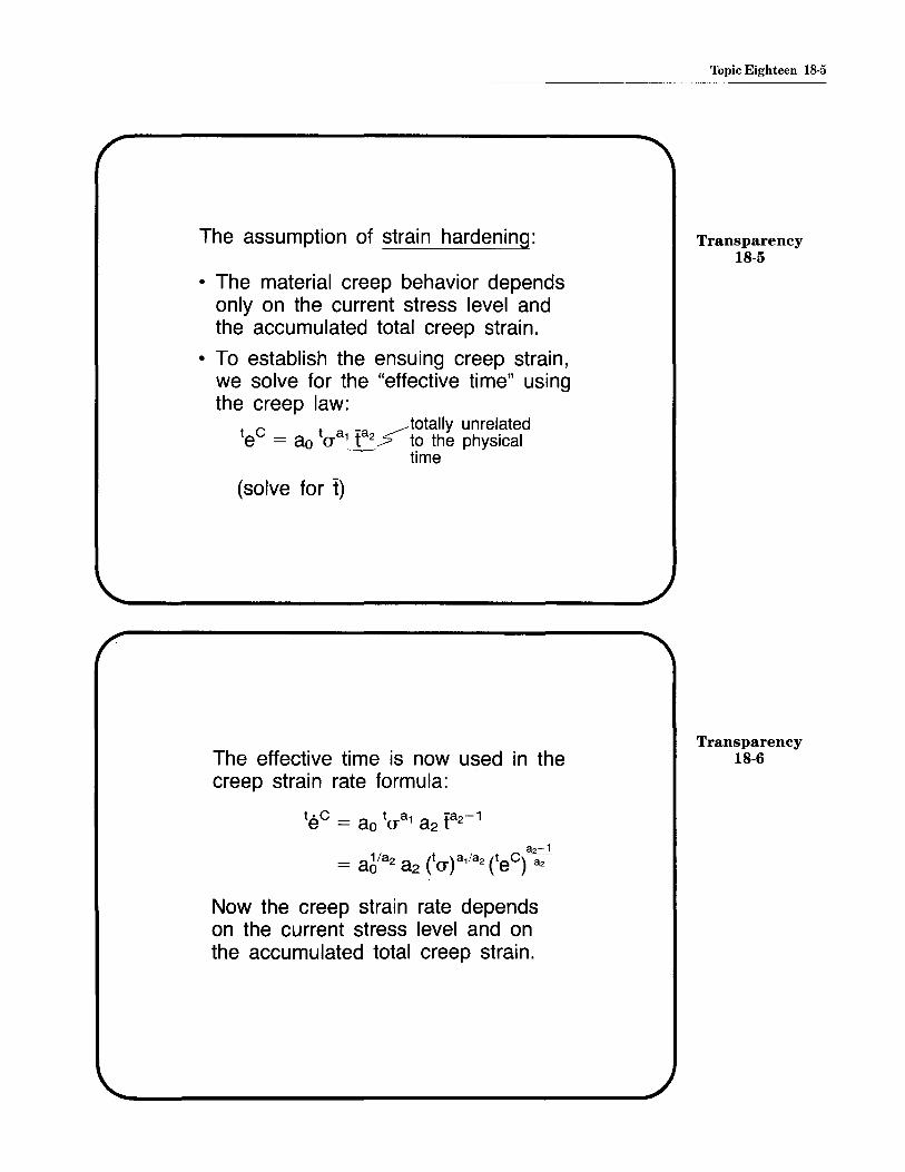
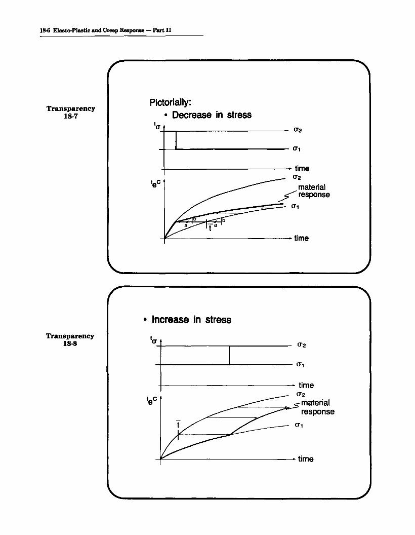
• Assumption of creep strain hardening for varying stresssituations
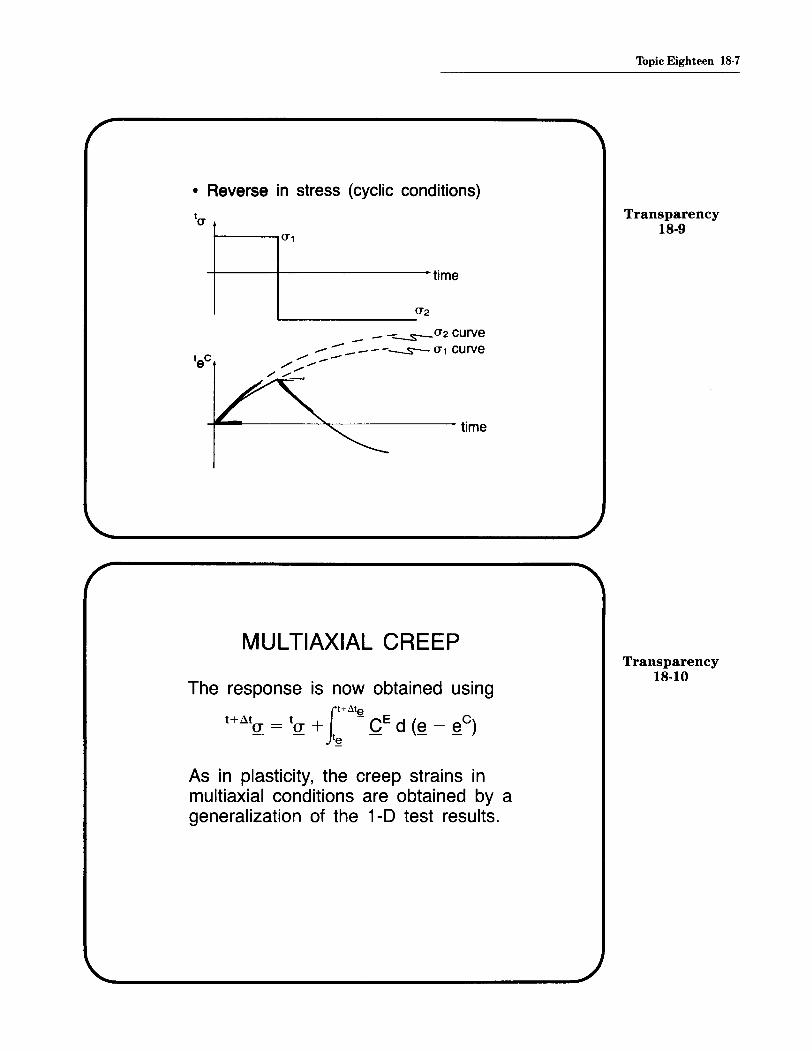
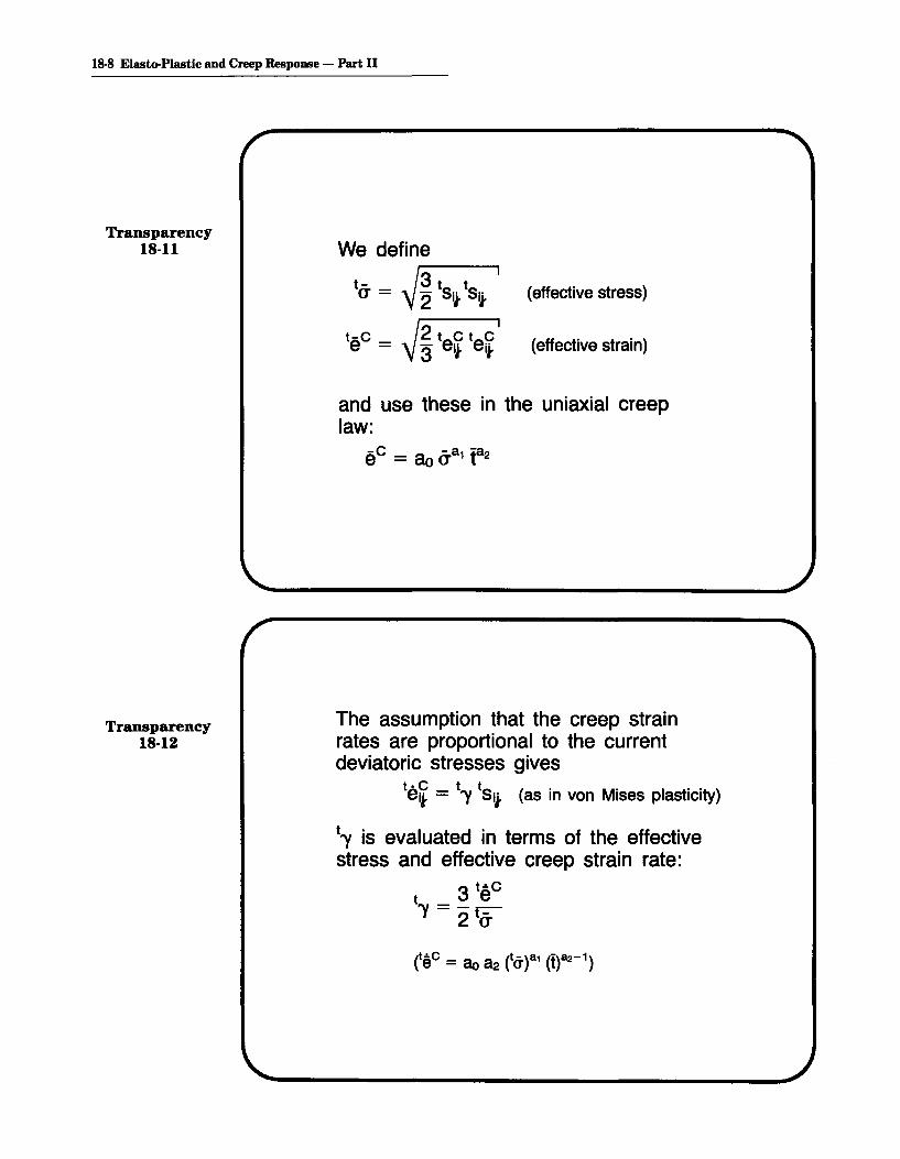
• Creep in multiaxial stress conditions, use of effectivestress and effective creep strain
• Explicit and implicit integration of stress
• Selection of size of time step in stress integration
• Thermo-plasticity and creep, temperature-dependency ofmaterial constants
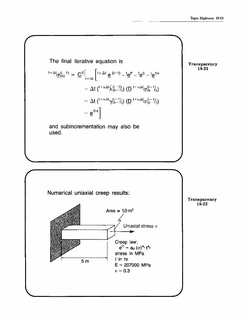
• Example analysis: Numerical uniaxial creep results
• Example analysis: Collapse analysis of a column withoffset load
• Example analysis: Analysis of cylinder subjected to heattreatment
Section 6.4.2
The computations in thermo-elasto-plastic-creep analysis are describedin
Snyder, M. D., and K. J. Bathe, "A Solution Procedure for Thermo-Elastic-Plastic and Creep Problems," Nuclear Engineering and Design, 64,49-80, 1981.
Cesar, F., and K. J. Bathe, "A Finite Element Analysis of QuenchingProcesses," in Numerical Methods jor Non-Linear Problems, (Taylor,C., et al. eds.), Pineridge Press, 1984.
18-2 Elasto-Plastic and Creep Response - Part II
References:(continued)
The effective-stress-function algorithm is presented in
Bathe, K. J., M. Kojic, and R. Slavkovic, "On Large Strain Elasto-Plasticand Creep Analysis," in Finite Element Methods for Nonlinear Problems (Bergan, P. G., K. J. Bathe, and W. Wunderlich, eds.), SpringerVerlag, 1986.
The cylinder subjected to heat treatment is considered in
Rammerstorfer, F. G., D. F. Fischer, W. Mitter, K. J. Bathe, and M. D.Snyder, "On Thermo-Elastic-Plastic Analysis of Heat-Treatment Processes Including Creep and Phase Changes," Computers & Structures,13, 771-779, 1981.
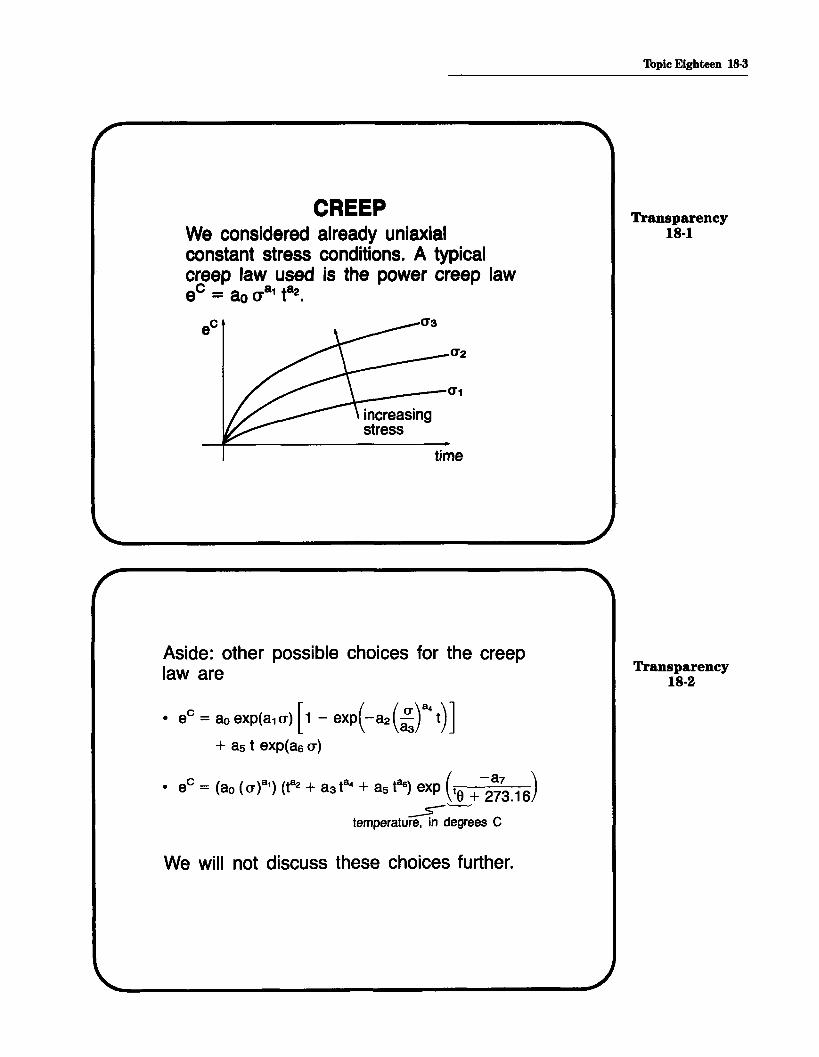
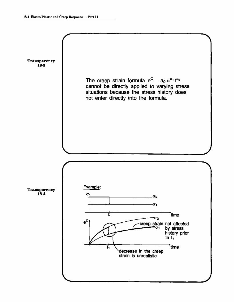
CREEPWe considered already uniaxialconstant stress conditions. A typicalcreep law used is the power creep laweO = ao (181 t~.
time
Aside: other possible choices for the creeplaw are
The results are obtained using twosolution algorithms:
• ex = 0, (no subincrementation)• ex = 1, effective-stress-function
procedure
In all cases, the MNO formulation isemployed. Full Newton iterationswithout line searches are used with
ETOL=0.001RTOL=0.01RNORM = 1.0 MN
Transparency18-24
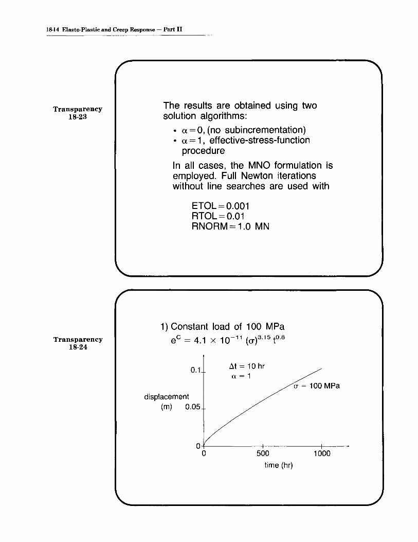
1) Constant load of 100 MPaeC = 4.1 x 10~11 (a)3.15 to.8
0.1 ~t = 10 hra=1
(J' = 100 MPa
displacement(m) 0.05
1000500
time (hr)
0+-------+------+----o
Topic Eighteen 18-15
Transparency18-25
at = 10 hr<x=1
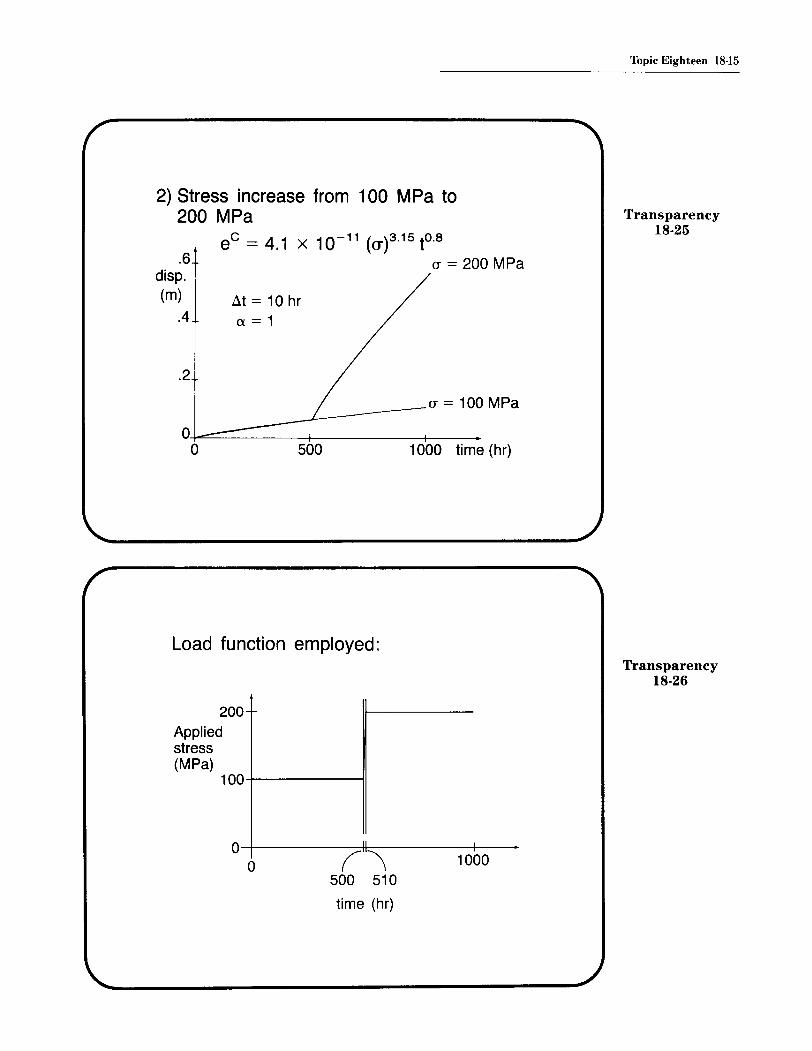
2) Stress increase from 100 MPa to200 MPa
eC = 4.1 x 10⁻¹¹ (cr)3.15 to.8
(J = 200 MPa.6disp.(m)
.4
.2
1000 time (hr)5000-+-==---- ----+ -+-__
o
(J = 100 MPaL---~
Load function employed:Transparency
18-26
200Appliedstress(MPa)
100+-------i1
1000O-+---------,H:-II -----+---
o (\500 510
time (hr)
18-16 Elasto-Plastic and Creep Response - Part II
~t = 10 hr(1=1
0.1disp.(m)0.0
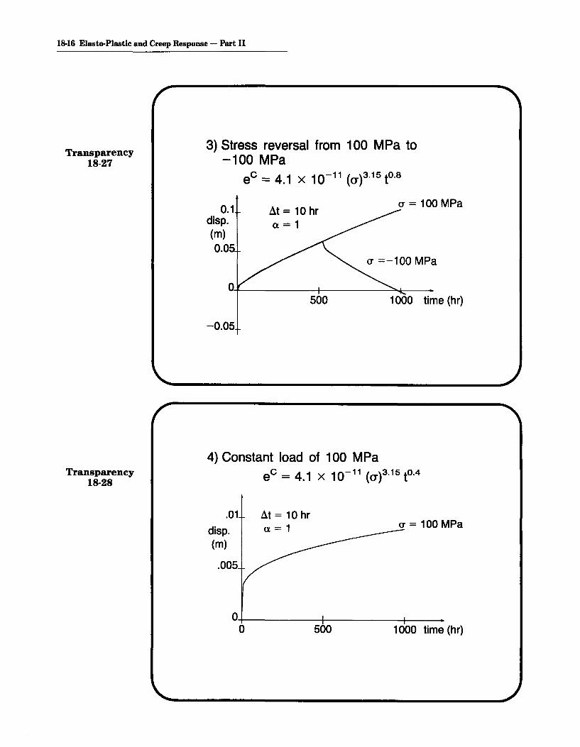
3) Stress reversal from 100 MPa to-100 MPa
eC = 4.1 x 10⁻¹¹ (cr)3.15 to.8
(J' = 100 MPa
Transparency18-27
500 1000 time (hr)
-0.05
Transparency18-28
4) Constant load of 100 MPaeC = 4.1 x 10⁻¹¹ (cr)3.15 t°.4
.01
disp.(m)
.005
~t = 10 hr(1=1 (J' = 100 MPa
1000 time (hr)500
0+- --+ -+-__
a
Topic Eighteen 18-17
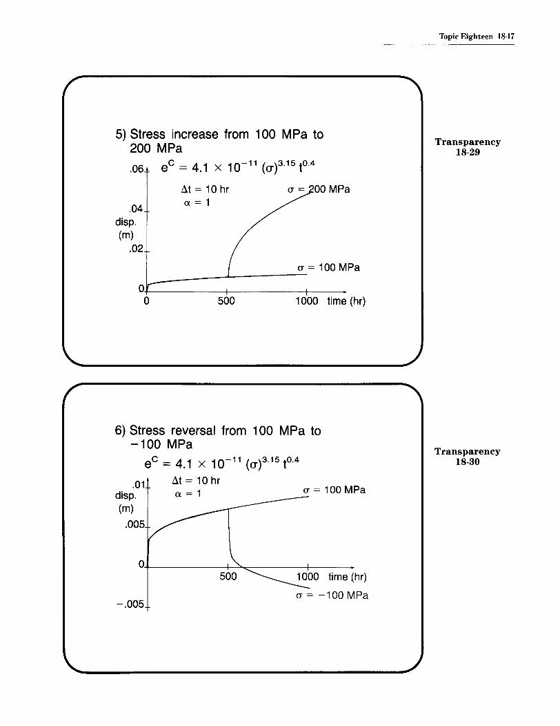
Transparency18-29
(T = 100 MPa
5) Stress increase from 100 MPa to200 MPa.06 eC = 4.1 x 10⁻¹¹ (cr)3.15 t°.4
8t=10hrex = 1
.04disp.(m)
.02
1000 time (hr)500
0,+-- --+ +- __
o
(T = 100 MPa
6) Stress reversal from 100 MPa to-100 MPa
eC = 4.1 x 10⁻¹¹ (cr)3.15 t°.4.01 8t = 10 hr
disp. ex = 1(m)
.005
Transparency18-30
O'+- -+~;;;:::__----+-------
1000 time (hr)
(T = -100 MPa-.005
18-18 Elasto-Plastic and Creep Response - Part II
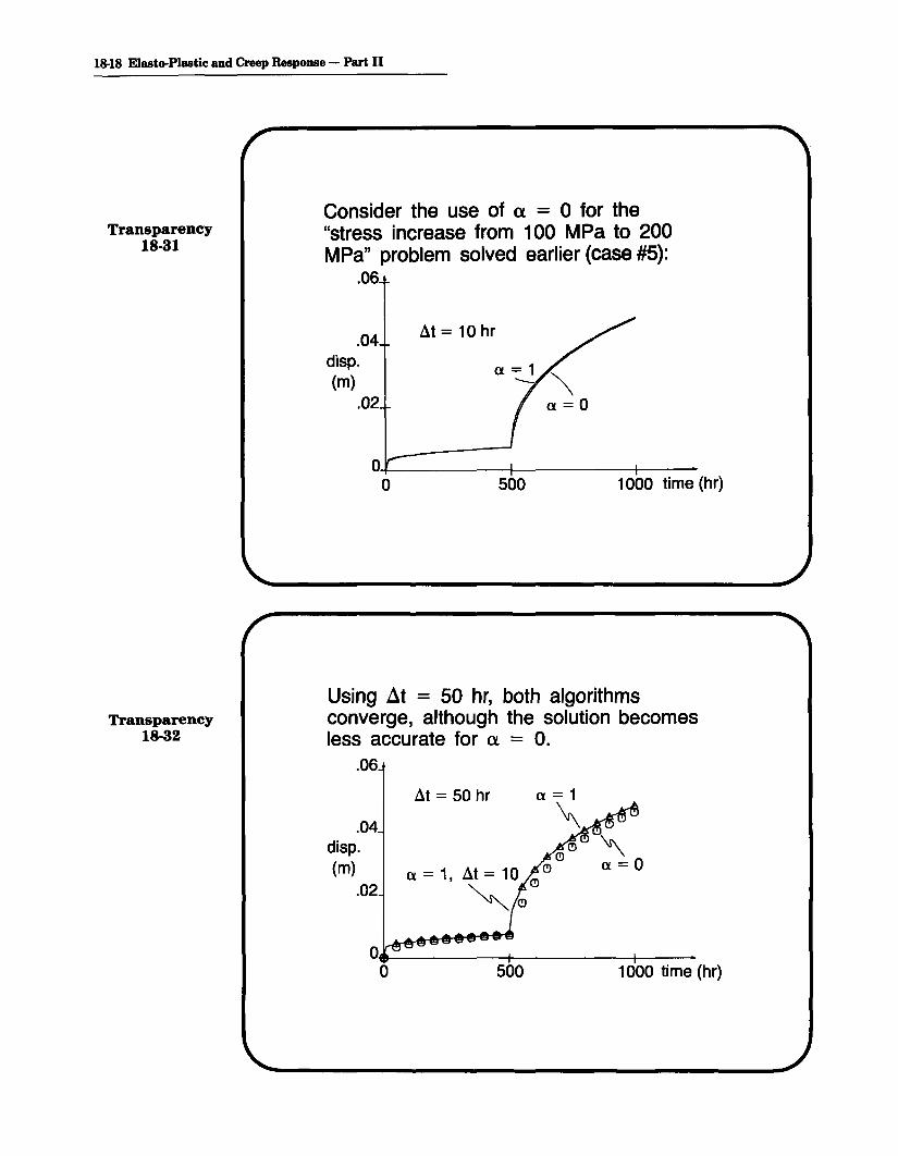
Transparency18-31
Consider the use of a = 0 for the"stress increase from 100 MPa to 200MPa" problem solved earlier (case #5):
.06
.04disp.(m)
.02
~t = 10 hr
1000 time (hr)500
0,+- -+ +-__o
Transparency18-32
Using dt = 50 hr, both algorithmsconverge, although the solution becomesless accurate for a - O.
.06
.04disp.(m)
.02
~t = 50 hr
(!)(!)
(!)
<X = 1 ~t = 10 (!), (!)
~ (!)
1000 time (hr)5000,_------+------4----o
Topic Eighteen 18-19
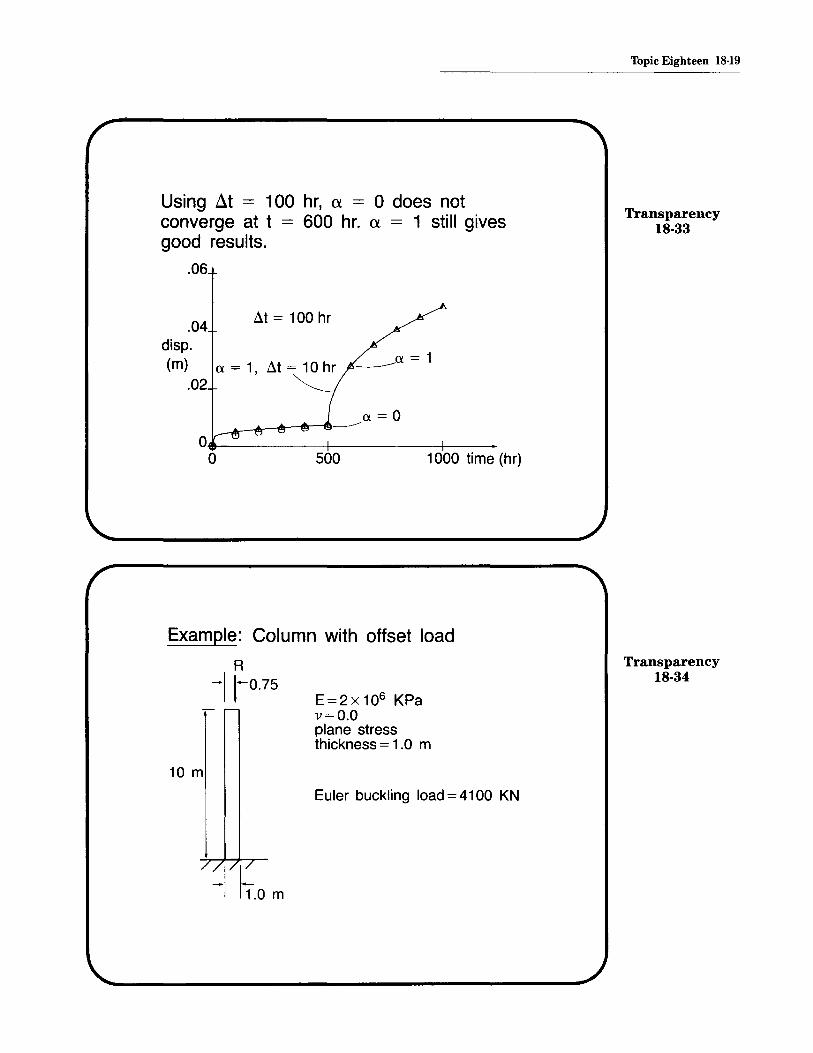
Using dt = 100 hr, (X = a does notconverge at t = 600 hr. (X = 1 still givesgood results.
.06
Transparency18-33
~t=100hr.04
disp.
(m) a = 1, ~t = 10 hr.02 ~
a=1--1000 time (hr)500
Oe--------t-~---__+_-o
E=2x10⁶ KPav=O.Oplane stressthickness = 1.0 m
Example: Column with offset load
R
-11-0.75
Transparency18-34
10 m
Euler buckling load = 41 00 KN
18-20 Elasto-Plastic and Creep Response - Part II
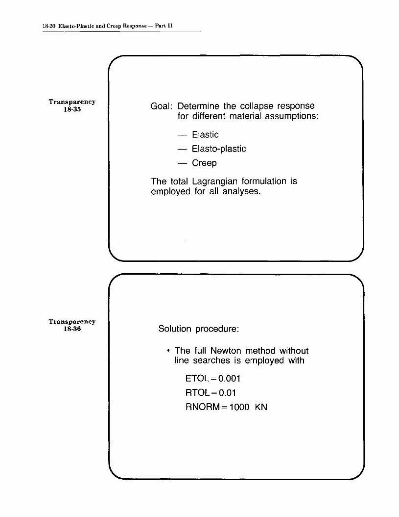
Transparency18-35
Transparency18-36
Goal: Determine the collapse responsefor different material assumptions:
Elastic
Elasto-plastic
Creep
The total Lagrangian formulation isemployed for all analyses.
Solution procedure:
• The full Newton method withoutline searches is employed with
ETOL=0.001
RTOL=0.01
RNORM = 1000 KN
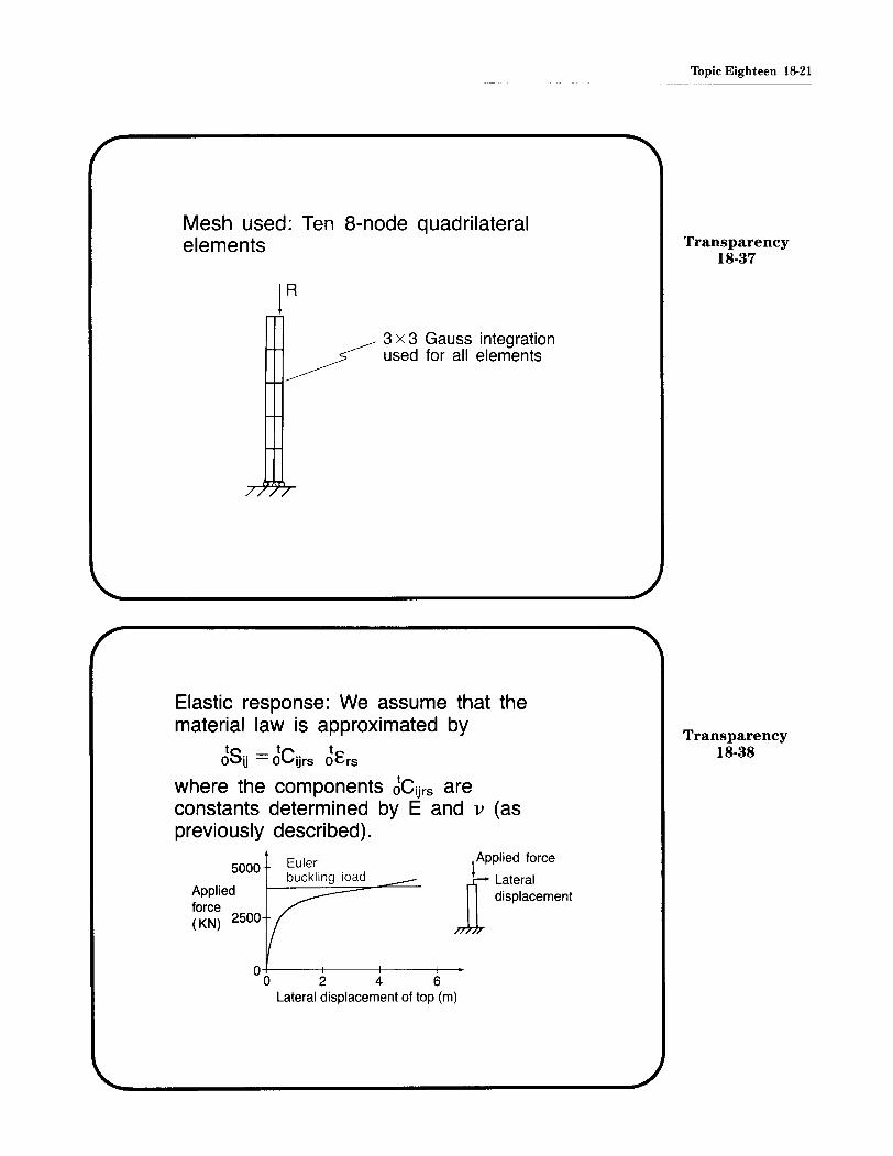
Mesh used: Ten 8-node quadrilateralelements
~ 3 x 3 Gauss integration~ used for all elements
Elastic response: We assume that thematerial law is approximated by
ts tc to ij = 0 ijrs OCrs
where the components JCijrS areconstants determined by E and v (aspreviously described).
Topic Eighteen 18·21
Transparency18-37
Transparency18-38
5000
Appliedforce(KN) 2500
Eulerbuckling ioad
tPPlied forcenLateraljJr displacement
O+-----t----+----+---a 2 4 6
Lateral displacement of top (m)
18-22 Elasto-Plastic and Creep Response - Part II
Transparency18-39
Transparency18-40
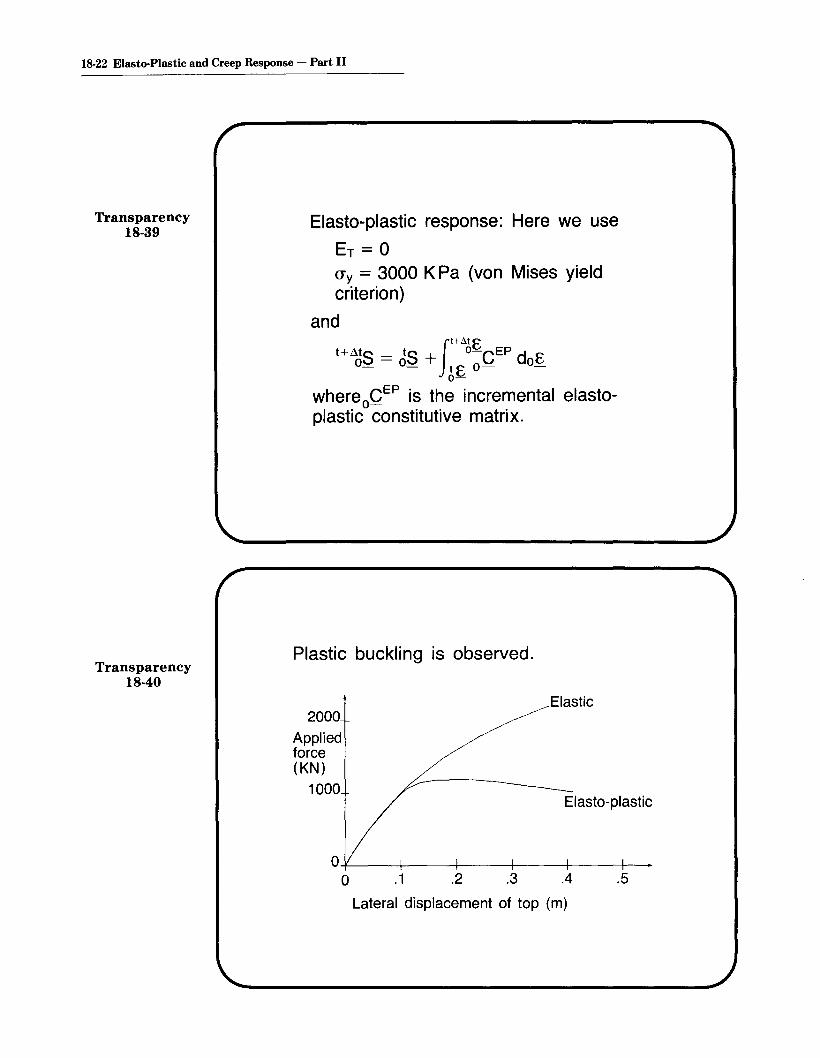
Elasto-plastic response: Here we use
ET = 0cry = 3000 K Pa (von Mises yieldcriterion)
and
JI+At E
t+LltS = cis + o-CEP doE0_ - tE 0- -
0-
whereoCEP is the incremental elastoplastic constitutive matrix.
Plastic buckling is observed.
Elastic2000
Appliedforce(KN)
1000Elasto-plastic
O+---t-----t---+---+---+---o .1 .2 .3 .4 .5
Lateral displacement of top (m)
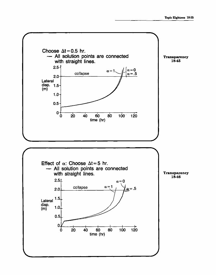
Creep response:
• Creep law: eC = 10-16(cr)3 t (t inhours)No plasticity effects are included.
• We apply a constant load of 2000K N and determine the time history ofthe column.
• For the purposes of this problem, thecolumn is considered to havecollapsed when a lateral displacementof 2 meters is reached. Thiscorresponds to a total strain of about2 percent at the base of the column.
We investigate the effect of differenttime integration procedures on theobtained solution:
• Vary At (At = .5, 1, 2, 5 hr.)
• Vary ex (ex=O, 0.5, 1)
'Ibpic Eighteen 18-23
Transparency18-41
Transparency18-42
18-24 Elasto-Plastic and Creep Response - Part II
Transparency18-43
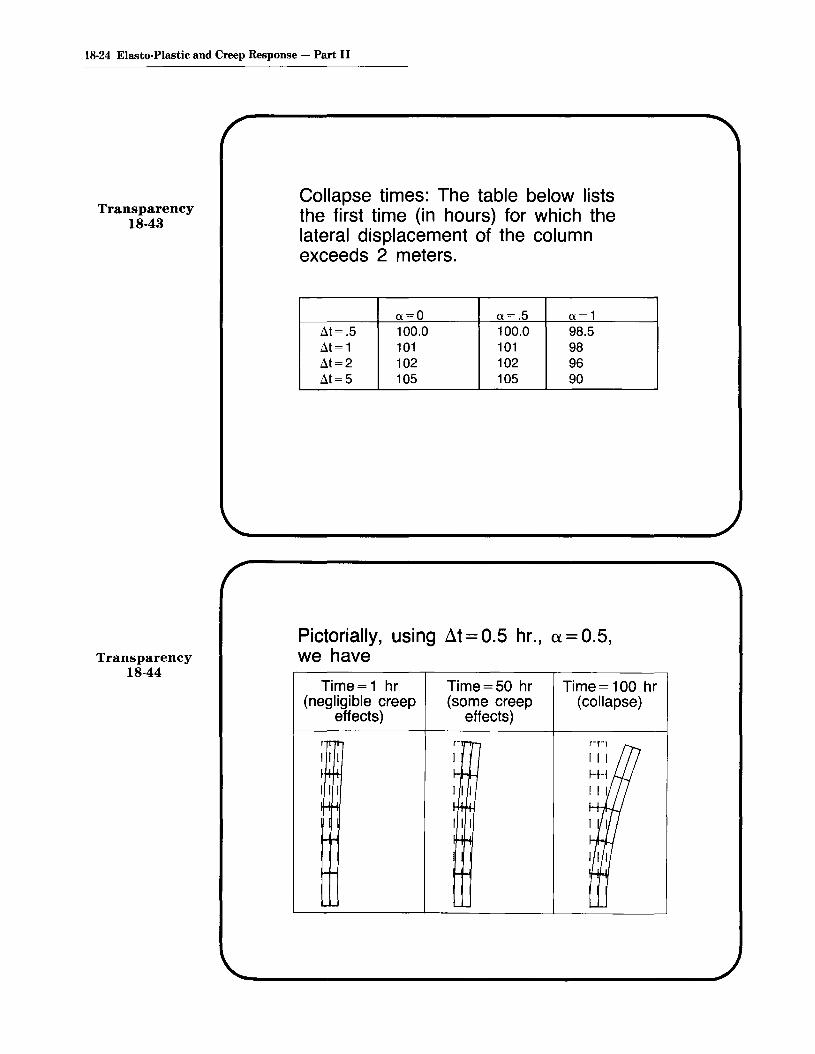
Collapse times: The table below liststhe first time (in hours) for which thelateral displacement of the columnexceeds 2 meters.
• As the time step is reduced, thecollapse times given by ex = 0,ex = .5, ex = 1 become closer. Forat = .5, the difference in collapsetimes is less than 2 hours.
• For a reasonable choice of timestep, solution instability is not aproblem.
r
I=-"T
II
zf-rl~2Ra
I I IS: : S!IL..............--JIL-IL.....L..I..L.IL..&II~I..LIu..111'"'r',~
Ra = 25 mm ~
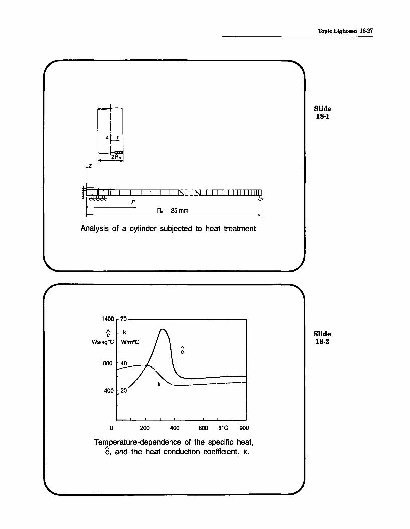
Analysis of a cylinder subjected to heat treatment
Topic Eighteen 18-27
Slide18-1
1400 70
/\ k SlidecWs/kgDC W/mDC 18-2
/\c
800
400 20
o 200 400 600 ODC 900
Temperature-dependence of the specific heat,~, and the heat conduction coefficient, k.
18-28 Elasto·Plastic and Creep Response - Part II
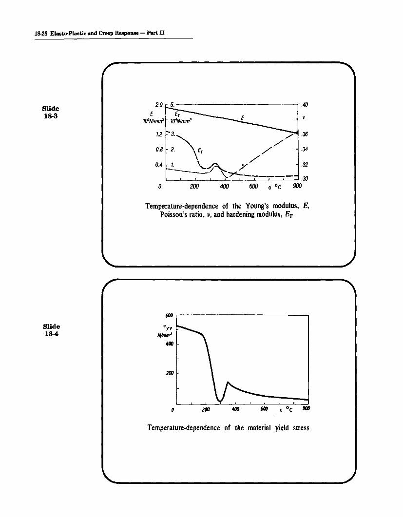
Slide18-3
1.2
0.4
----------------, .40
v
.32
Temperature-dependence of the Young's modulus, E,Poisson's ratio, II, and hardening modulus, ET
600 ,..-----------------..
Slide18-4
200
o
Temperature-dependence of the material yield stress
Thpic Eighteen 18-29
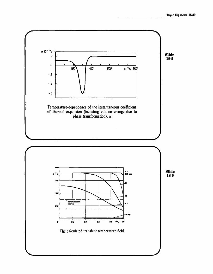
Slide18-5
600 0 °c 900o
-2
-6
-4
a 1O-5oc-/r------- --.
2
Temperature-dependence of the instantaneous coeffiCientof thermal expansion (including volume change due to
phase transformation), a
,.,..-------------------,
1SII+---+------t---+---"~_+---\--I
_+---+------t---""''''<:::'""""-+--_+*-----'I
t·IU'5_
D.5
J.j
Slide18-6
--fI fI.l fl.• (J.f II r/Ra Lfl
The calculated transient temperature field
18-30 Elasto-Plastic and Creep Response - Part II
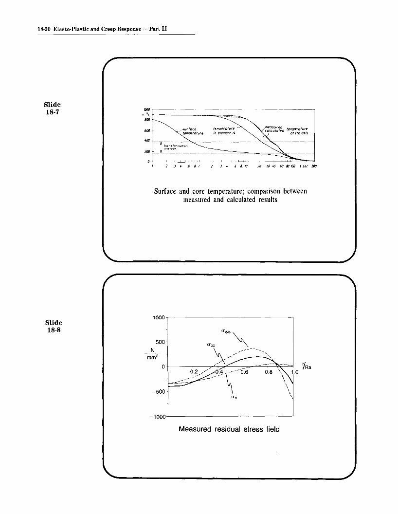
Slide18-7
1000 r-------------------------~
e °c r----------=-==~_600
10 3D to 60 txI 100 t.oc JOt)
temperatureIn element "
2 J. 6810
surfacet~mperaturl
1 J. 6 8 1
I§ranSformar-;;;: --------mr~rval
--------====~~=--
600
100
Surface and core temperature; comparison betweenmeasured and calculated results
Slide18-8
1000..----------------------,
500
Nmm2
-500Urr
-1000-'------------------~
Measured residual stress field
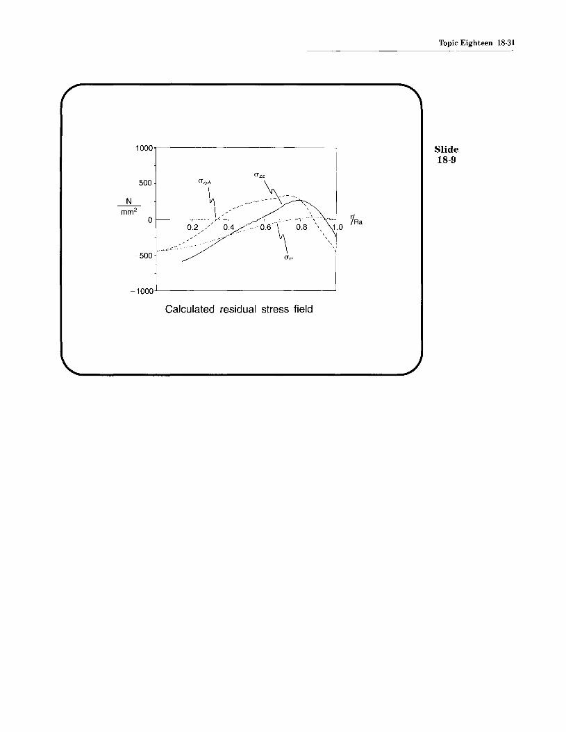
1000.,-------------------,
Topic Eighteen 18-31
Slide18-9
500
o
-500
\\
\
\ 1Ra0.8 " 1.0
\\
\\
\
-1000.L-------------------'
Calculated residual stress field
MIT OpenCourseWare http://ocw.mit.edu
Resource: Finite Element Procedures for Solids and Structures Klaus-Jürgen Bathe
The following may not correspond to a particular course on MIT OpenCourseWare, but has been provided by the author as an individual learning resource.
For information about citing these materials or our Terms of Use, visit: http://ocw.mit.edu/terms.