Page 1
MODELING OF SYNCHRONOUS GENERATOR AND FULL-SCALE
CONVERTER FOR DISTRIBUTION SYSTEM LOAD FLOW ANALYSIS
by
Inderpreet Singh Wander
Master of Technology, Electrical Engineering, P. A. University, India, 2000
A thesis
presented to Ryerson University
in partial fulfillment of the
requirements for the degree of
Master of Applied Science
in the program of
Electrical and Computer Engineering
Toronto, Ontario, Canada, 2011
© Inderpreet Singh Wander 2011
Page 3
iii
AUTHOR'S DECLARATION
I hereby declare that I am the sole author of this thesis or dissertation.
I authorize Ryerson University to lend this thesis or dissertation to other institutions or
individuals for the purpose of scholarly research.
_____________________________
(Inderpreet Singh Wander)
I further authorize Ryerson University to reproduce this thesis or dissertation by photocopying or
by other means, in total or in part, at the request of other institutions or individuals for the
purpose of scholarly research.
_____________________________
(Inderpreet Singh Wander)
Page 4
iv
ABSTRACT
MODELING OF SYNCHRONOUS GENERATOR AND FULL-SCALE CONVERTER
FOR DISTRIBUTION SYSTEM LOAD FLOW ANALYSIS
Inderpreet Singh Wander
Masters of Applied Science, Electrical and Computer Engineering, Ryerson University, 2011
Environmental awareness and the need to reduce greenhouse gas emissions have promoted the
use of green energy sources such as Wind Energy Conversion Systems (WECS). The Type 4
Permanent Magnet Synchronous Generator (PMSG) with a Full-Scale Converter has grown to be
a preferred choice among WECS. Conventionally these WECS are modeled as fixed PQ
injections in distribution system analysis studies and for that reason they are not accurately
represented. This inaccuracy is accentuated given the large-scale of integration of WECS. To
overcome this limitation, this thesis proposes to develop a steady-state model for the Type 4
PMSG WECS to be used in unbalanced three-phase distribution load flow programs. The
proposed model is derived from the analytical representation of its six main components: (1) the
wind turbine, (2) the synchronous generator, (3) the diode-bridge rectifier, (4) voltage source
inverter, (5) the dc-link with a boost converter that connects them, and (6) control mode action.
This proposed model is validated through mathematical analysis and by comparing with a
Matlab/Simulink model. Subsequently, the proposed model is integrated into a three-phase
unbalanced load flow program. The IEEE 37-bus test system data is used to benchmark the
results of the power flow method.
Page 5
v
ACKNOWLEDGMENTS
I express my deepest gratitude and appreciation to my supervisors, Dr. Bala Venkatesh of
Ryerson University and Dr. Vijay K. Sood of UOIT for their continuous guidance,
enlightenment, valuable instruction, encouragement and exceptional support throughout the
period of this research and Masters degree.
I gratefully acknowledge the financial support by the NSERC grant to Dr. Bala
Venkatesh and Dr. Vijay K. Sood.
My special thanks go to Dr. Alexandre Nassif, Post Doctoral Fellow at Ryerson
University for providing his valuable suggestion in improvement of this thesis.
I would like to express my thankfulness to faculty members and staff of Electrical and
Computer Engineering department of Ryerson University.
I will always remember all my friends in the Power and Energy Analysis Research
Laboratory, especially Amit, Bhanu, Inderdeep and Syed for the technical conversations,
exchange of ideas and moral support during my study at Ryerson University
I also thank my family and friends for their support and encouragement.
My deepest gratitude goes to my parents who have always provided unconditional
support. Thanks also go to my sister and brother-in-law.
Last but not least, my special thanks to my wife and two lovely kids for their love and
encouragement which has enabled me to complete this thesis.
Page 6
vi
TABLE OF CONTENT
Chapter Title Page
Title Page i
Author’s Declaration iii
Abstract iv
Acknowledgement v
Table of Content vi
List of Tables ix
List of Figures x
List of Abbreviations xi
Nomenclature xiii
1. Introduction 1
1.1 Background 1
1.2 Review of Related Research 3
1.3 Objective and Contributions of this Research and Thesis Outline 5
2. Wind Energy Systems 7
2.1 Wind Energy Conversion Systems 7
2.2 Classification 8
2.2.1 Aerodynamic Power Control 8
2.2.2 Speed Control 9
2.2.2.1 Fixed-speed WECS 9
2.2.2.2 Variable-speed WECS 10
2.3 Synchronous Generator and Full-Scale Converter WECS 13
2.3.1 Structure 13
2.3.2 Operation 14
Page 7
vii
3. Proposed Model of WECS 14
3.1 Model 16
3.1.1 Wind Turbine Model 17
3.1.2 Synchronous Generator Model 17
3.1.3 Three Phase Diode Bridge Rectifier Model 18
3.1.4 Boost Converter Model 19
3.1.5 Voltage Source Inverter 20
3.1.6 Control Mode Action 20
3.1.7 Proposed Complete Type 4 Generator Model Algorithm 20
3.2 Validation 20
4. New Load Flow approach with the Proposed Type 4 WECS Model 24
4.1 Load Flow Method Description 24
4.2 Test System Description 29
4.3 WECS Model in Load flow Analysis – Two Approaches 31
4.3.1 Conventional Load Flow Approach with the Conventional Type 4 WECS
Model (LF-1) 32
4.3.2 New Load Flow Approach with the Proposed Type 4 WECS Model (LF-2) 32
4.3.3 Results and Comparisons of Power Flow Methods 33
5. Conclusions and Suggestions for Future Research 37
5.1 Conclusions 37
5.2 Suggestions for Future Research 38
References 39
Appendices 40
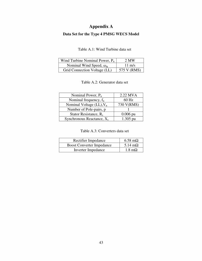
Appendix A: Data Set for the Type 4 PMSG WECS Model 43
Appendix B: Load Models Description with General Equations 44
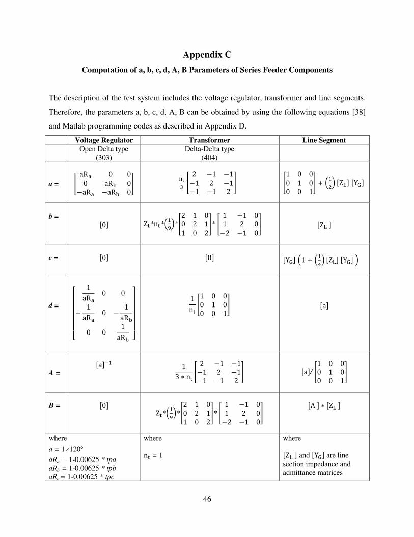
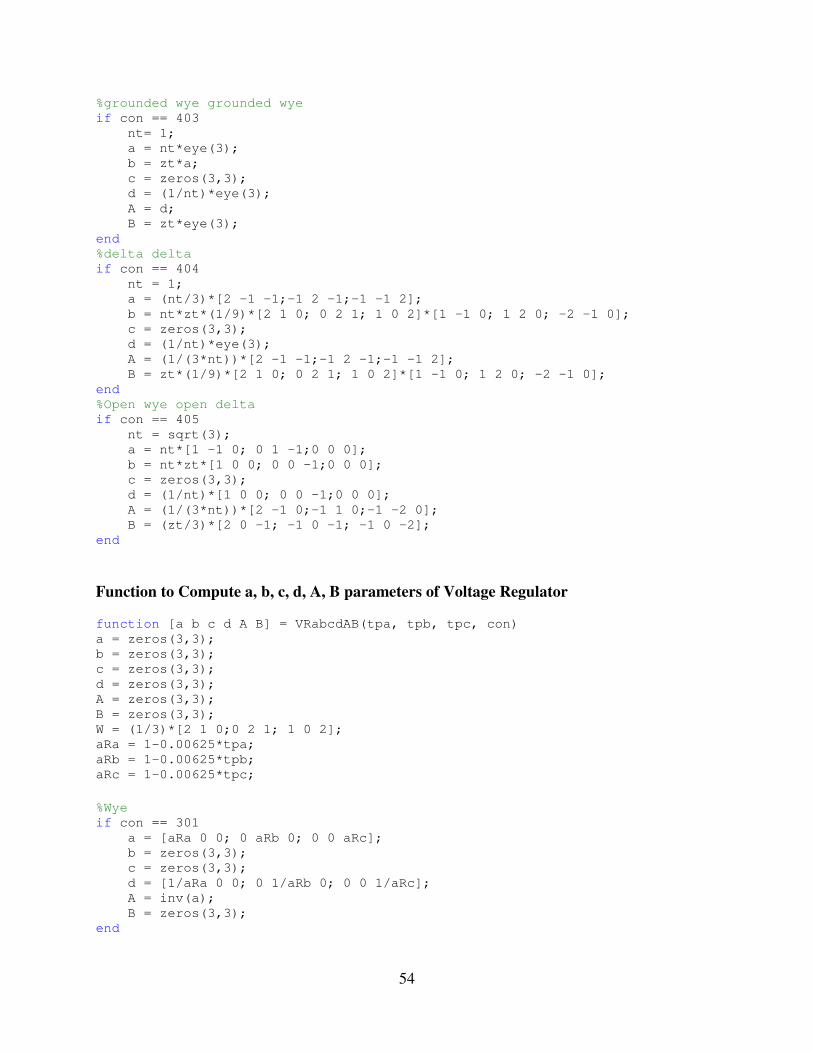
Appendix C: Computation of a, b, c, d, A, B Parameters of Series Feeder Components 46
Page 8
viii
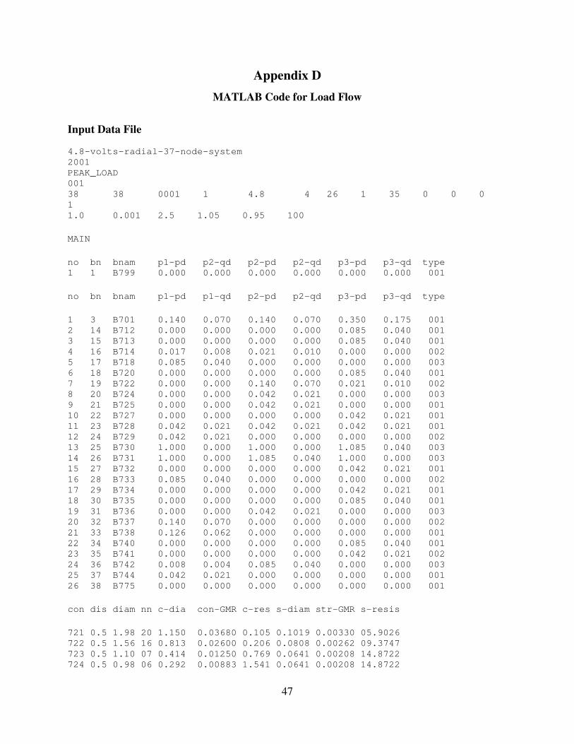
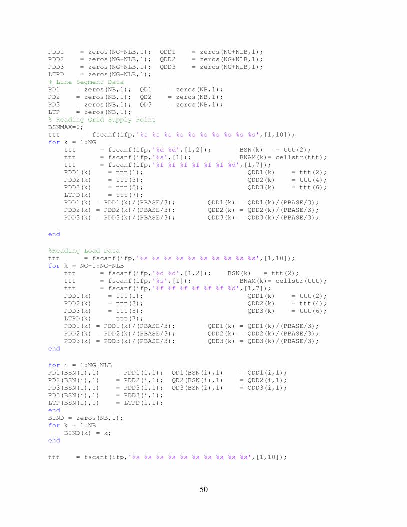
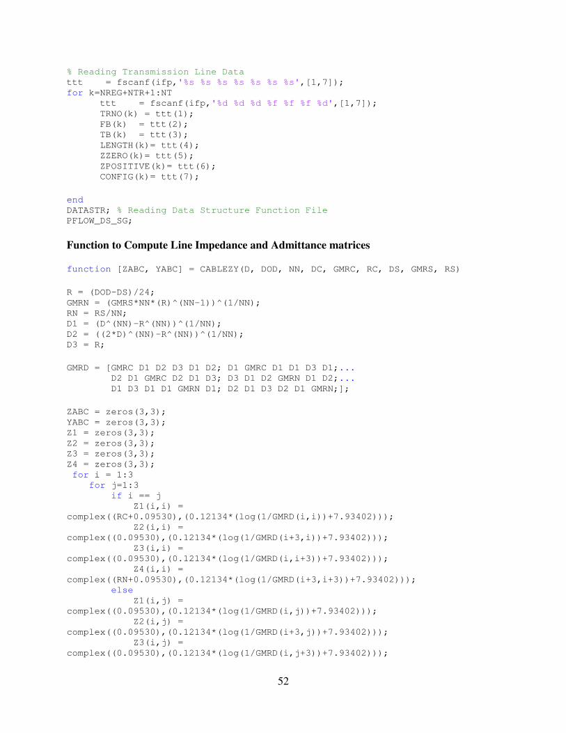
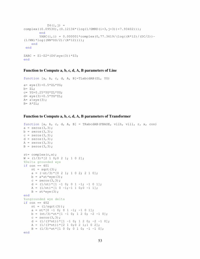
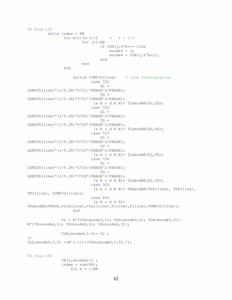
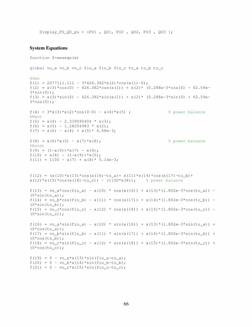
Appendix D: MATLAB Code for Load Flow 47
Appendix E: MATLAB Code for Proposed Type 4 Model 65
Page 9
ix
LIST OF TABLES
Table 3.1: Results from both models for the Type 4 WECS 22
Table 4.1: Comparison of results from both Load Flow methods for the IEEE 37-bus test
system 34
Table 4.2: Comparison of voltages and powers at the bus connecting the WECS for both
Load Flow methods 36
Table A.1: Wind Turbine data set 43
Table A.2: Generator data set 43
Table A.3: Converter data set 43
Page 10
x
LIST OF FIGURES
Figure 2.1: A generic Wind Energy Conversion System 7
Figure 2.2: Synchronous generator and full-scale converter WECS 13
Figure 3.1: Proposed equivalent model for the Type 4 WECS 16
Figure 3.2: Type 4 WECS model in Matlab-Simulink 22
Figure 4.1: Flowchart of Load Flow using conventional Ladder Iterative Technique 26
Figure 4.2: WECS connection to the IEEE 37-bus test system 30
Figure 4.3: Flowchart of Load Flow with Ladder Iterative Technique 31
Figure 4.4: WECS modeled as a fixed PQ load 32
Figure 4.5: Proposed WECS model integrated in the Load Flow solution 33
Figure 4.6: Comparison of line to line voltage a-b for both Load Flow approaches 35
Figure B.1: Delta connected load 44
Page 11
xi
LIST OF ABBREVIATIONS
AC Alternating current
CanWEA Canadian Wind Energy Association
DC Direct Current
DFIG Doubly Fed Induction Generator
DG Distributed Generation
DS Distribution System
ERR Error Value
EMF Electromotive Force
GW Giga Watts
GWEC Global Wind Energy Council
GSC Generator- Side Converter
HAWT Horizontal Axis Wind Turbine
IEEE Institute of Electrical and Electronics Engineers
IGBT Insulated Gate Bi-polar Junction Transistor
IT Iteration Number
KCL Kirchhoff Current Law
KVA Kilo Volt Ampere
KVL Kirchhoff Voltage Law
LF Load Flow
MW Mega Watts
NSC Network- Side Converter
PE Power Electronics
PMSG Permanent Magnet Synchronous Generator
PWM Pulse Width Modulation
TOL Tolerance
TS Transmission System
VAWT Vertical Axis Wind Turbine
VSC Voltage Source Converter
Page 12
xii
VSI Voltage Source Inverter
WECS Wind Energy Conversion Systems
WEG Wind Electric Generator
WF Wind Farm
WG Wind Generator
WT Wind Turbine
WRIG Wound Rotor Induction Generator
WRSG Wound Rotor Synchronous Generator
SG Synchronous Generator
Page 13
xiii
NOMENCLATURE
A Swept area of the rotor (m2)
β Blade pitch angle (°)
Cp Power coefficient
ωwind Wind speed (m/s)
ρ Air density (kg/m3)
PWind Power available in wind (W)
Pm Mechanical power developed by the wind turbine (W)
λ Tip speed ratio
f Frequency (Hz)
N Number of coil turns
ωe Electrical speed (radians/s)
ωm Mechanical speed(radians/s)
p Number of pairs of poles of the synchronous generator
Rs Generator winding resistance (Ω)
Xs Generator winding reactance (Ω)
E Induced electromotive force (V)
I_ Generator current in phase ph (A)
Generator magnetic flux (Wb)
φ_ Generator voltage phase angle
θ_ Generator current phase angle
V_ Generator terminal voltage of phase ph (V)
VLL Generator line-to-line output voltage (V)
Page 14
xiv
Vdcr Rectifier output DC voltage (V)
Idcr Rectifier output DC current (A)
IS1 Fundamental component of the generator stator current (A)
Pdci DC power flowing out of rectifier (W)
R Rectifier losses(Ω)
V DC voltage across the boost converter (V)
V DC voltage output at the boost converter (V)
D Boost converter duty cycle
Idcb DC current output from the boost converter (A)
Pdcb DC power output from the boost converter (W)
R Boost converter losses (Ω)
V_ Phase voltage at the VSI terminal (V)
ma VSI PWM modulation index
V_ Three-phase VSI output voltage (V)
φ_ Angle of each VSI output phase voltage
θ_ Angle of each VSI output phase current
R VSI output resistance including losses (Ω)
X VSI output reactance (Ω)
Po_ph VSI phase real power output (W)
Q_ VSI phase reactive power output (Var)
Page 15
1
Chapter 1
Introduction
1.1 Background
The deregulation of electric markets has led to the emergence of distributed generation
(DG). These units comprise renewable and non-renewable sources. With the increased awareness
for environmental preservation and the drive to reduce greenhouse gas emissions, there has been
a significant shift towards renewable energy sources, leading most people to associate the
acronym DG with such. Among those, wind energy, being clean and commercially competitive,
has been one of the most popular choices. A large number of Wind Energy Conversion Systems
(WECS) are already in operation and many new systems are being planned [1]-[3]. According to
the Global Wind Energy Council (GWEC), the total capacity of wind power operating in the
world reached 194.4 GW in 2010, an increase of 22.5 % from 159.2 GW in 2009 [4]. In Canada
alone, the installed capacity is 4009 MW in 2010, an increase of 17% from 2009 [5]. With many
government incentives across most of its provinces, it is expected that wind power installation
will experience steady growth in the forthcoming years.
Wind power conversion differs from other conventional sources due to (1) the
construction of WECS, which most commonly use power electronics-based converters, resulting
in the application of different topologies, (2) the unpredictable nature of wind power, which is
intermittent and uncertain, and (3) the change from a passive distribution network into an active
one with multiple energy sources and bidirectional power flow1. Due to these factors associated
with wind power, it interacts differently with the power system network. The most obvious
challenge that it can create is the dependence of the injected power on the wind speed. Therefore,
fluctuations in wind velocity can affect branch power flows, bus voltages, reactive power
injections, system balancing, frequency control, power system dynamics and stability. In
addition, it can also affect the power quality by introducing harmonics and flicker, due to the
1 Note that the reverse flow of power is not unique to wind energy conversion, but can take place in any scenario
where DGs are connected to distribution feeders.
Page 16
2
switching actions of the power electronics converters, and can also affect protection systems due
to the increase in fault levels [1]-[2].
Due to the aforementioned, different grid codes have been developed for wind power
integration so as to fulfill technical requirements such as frequency and voltage control, active
and reactive power management and fast response during transient and dynamic situations. To
satisfy these requirements and because of other technical and economical reasons, different
topologies of WECS have been developed. Variable-speed WECS are the favoured option due to
superior power extraction, controllable output power, quick response under transient and
dynamic situations, reduced mechanical stress and acoustical noise [1], [6], [7]. Variable-speed
WECS can apply Doubly-Fed Induction Generators (DFIGs or Type 3 generators) or
synchronous generators and full-scale converters (also referred to as Type 4 generators). While
DFIGs have gained popularity in recent years, Type 4 generators have been gradually capturing
the market [8]. More details on different WECS types are provided in Chapter 2.
Thus, electrical power systems are undergoing a change from a well-known and
developed topology to another new and partly unknown. The interaction of wind turbines with
electrical power systems is becoming more significant. With the rapid increase in the number of
WECS in power system, the effects of wind power on the grid need to be fully understood and
properly investigated. The steady-state investigation is done through Load Flow analysis, which
is an important tool in power system planning and operation. The objective of a load flow is to
determine the current flows on transmission lines (or distribution feeders) and transformers,
voltages on buses and to calculate power line losses [14]-[15]. This study is also important in the
planning and design of the interconnection of the wind farm to the system, to ensure that existing
scenarios are operated within their capabilities and new scenarios (after the installation of
WECS) are properly planned. The load flow is also commonly used to provide initial conditions
for dynamic and stability analyses.
To obtain accurate results in the load flow analysis and adequately investigate their
effects on the electric system, the detailed features of WECS must be included in the load flow
algorithms. Ideally, this integration should not impact the performance of the solution algorithm.
Page 17
3
1.2 Review of Related Research
With the growth of wind power in power systems, a large number of studies have been
done to investigate its behaviour and impact on the power system. Most of these studies are
performed to investigate the dynamic behaviour. Conversely, very few studies have been done to
understand the steady-state behaviour of wind turbines
In [11], comprehensive dynamic simulation models were implemented and advanced
control strategies were designed for different wind turbine concept which were claimed to
improve power system stability. The authors, in [12], have described the dynamic modelling and
control system of a direct-drive wind turbine which enabled the wind turbine to operate
optimally. In [13], converter driven synchronous generator models of various orders, which can
be used for simulating transients and dynamics in a very wide time range, were presented.
The power output of the wind generator depends on the characteristics of the turbine and
control systems. One of the important functions of the control systems is to determine the active
and reactive powers supplied by the wind turbine to the grid. Conversely, the performance of the
WECS is affected by the varying grid conditions. These conditions need to be considered when
developing steady-state models for WECS.
A previous number of studies have modeled WECS as a simple induction generator
equivalent circuit with very simple turbine characteristics [16]-[18]. In [16], two single-phase
steady-state models of asynchronous generators were presented. One is a constant PQ model, in
which active power is a function of wind speed. The other is a RX model, in which active and
reactive powers are calculated by using equivalent circuit parameters of induction machine. This
is claimed to be more accurate, with the advantage that the only input variable needed was the
wind speed. The authors of [17] have compared two models of induction generator. One is a
fixed PQ model whose reactive power is expressed as a function of WECS’s mechanical input.
The other is a fixed RX model, in which active and reactive power were calculated by using
equivalent circuit parameter. The developed models were incorporated into three-phase
distribution system load flow. A new approximate fixed PQ model of Asynchronous wind
Page 18
4
turbine was described in [18], in which mechanical power is the input variable and the reactive
power is calculated as a function of the machine parameters and the voltage of the machine.
The authors of [19] have proposed steady-state models for the Doubly Fed Induction
Generator (DFIG). These models ranged from a fixed PQ injection modeling approach to a more
detailed level of modeling. The DFIG is also modeled as fixed PV or RX model. In the RX fixed
model the wind speed was considered as input data, making the mechanical power as a function
of given wind data. The study was limited to a single-phase model and a load flow solution based
on the Newton-Raphson method.
As far as the Type 4 WECS is concerned, this WECS has been traditionally modeled by
utilities as a constant PQ or PV bus [20], [22], [24-[25]. In some cases it was modeled as a
single-phase system [21], [25] or as a three-phase balanced system [20]-[24].
In [20] and [24] different configurations were modeled as constant PQ and PV model,
depending on the control used, for balanced three-phase load flow analysis. Various components
of WECS were not considered in the models. In [21], steady-state models of different
configurations of WECS were developed for single-phase load flow. These were modeled as
fixed PQ and PV bus. Direct-Drive Synchronous Generator is then modelled as a PV bus in the
load flow study. With reactive power limits enforced, if the limit is reached, the PV bus is
converted to a PQ bus. These models do not consider the various components of whole WECS.
Different models of various DGs, including different configurations of Wind Turbines, were
developed in [22], with the claim that the traditional three-phase load low method was improved.
But details have not been provided. Another modeling variant was presented in [23]. In these
steady-state models of various types of WECS, the WECS components and losses have been
ignored. Single-phase models were developed in [25] for different configurations of WECS to be
used in the Newton-Raphson method-based load flow analysis. Variable-speed WTs were
modeled as constant PQ model. Therefore this technique also lacks modeling accuracy. In
addition, details of the asynchronous generator model is provided and not in the case of
synchronous generator.
Page 19
5
While such approaches were considered reasonable to represent a few generators under
balanced conditions, nowadays they are clearly inadequate to represent the Type 4 WECS given
the present and anticipated scale of penetration in distribution systems. Therefore, with the
noticeable acceptance of the Type 4 WECS by the market, it is visibly necessary to develop a
more accurate model to represent the technology in load flow studies.
1.3 Objective and Contribution of this Research and Thesis Outline
Despite the growing scale of integration of the Type 4 WECS, very little research has
been done towards developing an accurate model for distribution system planning and analysis
studies. Most of the WECS units are being connected in distribution networks, which are usually
unbalanced. Thus, with the anticipated large scale installation of Type 4 WECS, its accurate
modelling has become very important.
The main objective of this thesis is to propose a three-phase model for Type 4 WECS
representing all its components. The proposed model is validated by using Matlab-Simulink and
subsequently incorporated in a three-phase load flow program used to solve the IEEE 37-bus
unbalanced distribution system [39].
The main contributions of this research are those presented in Chapters 3 and 4.
The structure of this thesis is as follows:
Chapter 2 provides a background on wind energy conversion system along with their power
controls. A detailed analysis of the Type 4 topology is presented.
Chapter 3 presents the modeling of all WECS elements and the proposed algorithm to obtain its
complete model. This model is validated through time-domain simulations in Matlab-Simulink.
Chapter 4 presents the Load Flow solution using the ladder iterative technique with the
integration of both (1) the traditional WECS model, and (2) the proposed WECS model with the
Page 20
6
IEEE-37 bus distribution system. Finally the resulting errors from using the traditional WECS
model are quantified by comparing the results from both models.
Chapter 5 presents the conclusions and contributions of this thesis, as well as suggestions for
future work.
Page 21
7
Chapter 2
Wind Energy Conversion Systems
2.1 Wind Energy Conversion Systems
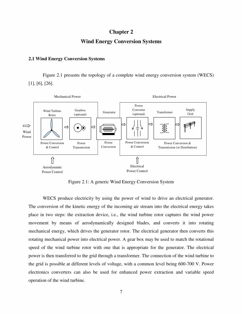
Figure 2.1 presents the topology of a complete wind energy conversion system (WECS)
[1], [6], [26].
Figure 2.1: A generic Wind Energy Conversion System
WECS produce electricity by using the power of wind to drive an electrical generator.
The conversion of the kinetic energy of the incoming air stream into the electrical energy takes
place in two steps: the extraction device, i.e., the wind turbine rotor captures the wind power
movement by means of aerodynamically designed blades, and converts it into rotating
mechanical energy, which drives the generator rotor. The electrical generator then converts this
rotating mechanical power into electrical power. A gear box may be used to match the rotational
speed of the wind turbine rotor with one that is appropriate for the generator. The electrical
power is then transferred to the grid through a transformer. The connection of the wind turbine to
the grid is possible at different levels of voltage, with a common level being 600-700 V. Power
electronics converters can also be used for enhanced power extraction and variable speed
operation of the wind turbine.
Generator
Power
Conversion
Mechanical Power
Wind
Power
Wind Turbine
Rotor
Power Conversion
& Control
Gearbox
(optional)
Power
Transmission
Aerodynamic
Power Control
Power Conversion &
Transmission (or Distribution)
Electrical Power
Power Conversion
& Control
Power
Converter
(optional) Transformer
Supply
Grid
Electrical
Power Control
Page 22
8
2.2 Classification
The development of various WECS concepts in the last decade has been very dynamic
and several new configurations have been developed. With the development of power converter
technologies, several different types of wind turbine configurations, using a wide variety of
electric generators, are available. One difference in the basic configuration is the vertical axis
wind turbine (VAWT) and horizontal axis wind turbine (HAWT). Today, the vast majority of
manufactured wind turbines apply the horizontal axis. Another major difference among WECS
concepts is the electrical design and control. So the WECS can be classified according to the
speed control ability, leading to WECS classes differentiated by generator speed, and according
to the power control ability, leading to WECS classes differentiated by the method employed for
limiting the aerodynamic efficiency above rated power. Input wind power control ability divides
WECS into three categories: Stall-controlled, Pitch-controlled, and Active-pitch controlled. The
speed control criterion leads to two types of WECS: Fixed-speed and Variable-speed [1], [6],
[26]. This chapter addresses most of the topologies widely in use today.
2.2.1 Aerodynamic Power Control
Power control ability refers to the aerodynamic performance of wind turbines. There are
different ways to control aerodynamic forces on the turbine rotor and thus to limit the power in
very high winds in order to avoid the damage to the wind turbine [1], [6], [26].
Passive Stall control
Input wind power is regulated by the aerodynamic design of the rotor blades. In this
design, the blades are fixed to the hub at a fixed angle. This design causes the rotor to stall (lose
power) when the wind speed exceeds a certain level. Thus, the aerodynamic power on the blades
is limited. This method is simple, inexpensive, and mostly used in fixed-speed WECS. This
arrangement causes less power fluctuations than a fast-pitch power regulation. On the negative
side, this method has lower efficiency at low wind speeds and has no assisted start-up.
Page 23
9
Pitch control (Active control)
Input wind power is controlled by feathering the blades. In this method, blades are turned
out or into the wind as the power output becomes too high or too low, respectively. Rotor blade
pitch is varied to control both the rotational speed and the coefficient of performance. At high
wind speeds the mean value of the power output is kept close to the rated power of the generator.
Thus, power is controlled by modifying the pitch-angle, which modifies the way the wind speed
is seen by the blade. This method has the advantages of good power control, assisted start-up and
emergency stop. This is the most commonly used in variable-speed wind turbines. But his
method suffers from extra complexity and higher power fluctuations at high wind speeds.
Active stall control
In this control method, the stall of the blade is actively controlled by pitching the blades.
The blade angle is adjusted in order to create stall along the blades. At low wind speeds the
blades are pitched similarly to a pitch-controlled wind turbine, in order to achieve maximum
extraction from the wind. At high wind speeds, i.e., above rated wind speeds, the blades go into a
deeper stall by being pitched slightly into the opposite direction to that of a pitch-controlled
turbine. Smoother limited power is achieved without high power fluctuations as in the case of
pitch-controlled wind turbines. This control type also compensates variations in air density. The
combination with pitch mechanism makes it easier to carry out emergency stops and to start up
the wind turbine.
Yaw control
Another control method is called the Yaw control, in which the entire nacelle is rotated
around the tower to yaw the rotor out of the wind. Due to its complexity, the Yaw control is less
utilized than other methods.
2.2.2 Speed Control
2.2.2.1 Fixed-speed WECS (the Type 1 WECS)
Fixed-speed WECS are electrically simple devices, consisting of an aerodynamic rotor
driving an Induction (Squirrel cage or wound rotor) generator which is directly connected
Page 24
10
through gearbox and shaft. The slip, and hence the rotor speed of generator, varies with the
amount of power generated. These rotor speed variations are, however, very small
(approximately 1 to 2 percent). Therefore, this WECS is normally referred to as a constant or
fixed speed system. The rotor speed is determined by the frequency of the supply grid, the gear
ratio and the number of pole-pairs of a generator, regardless of the wind speed. These are
designed to achieve maximum efficiency at one particular wind speed. At wind speeds above and
below the rated wind speed, the energy capture does not reach the maximum value. Fixed-speed
WECS are mechanically simple, reliable, stable, robust and well-proven. They have low cost
maintenance and electrical parts. Conversely, these suffer from the disadvantages of mechanical
stress, limited power quality control, and poor wind energy conversion efficiency.
2.2.2.2 Variable-speed WECS
As the size of WECS is becoming larger and the penetration of wind power in power
system is increasing, the inherent problems of fixed-speed WECS become more and more
pronounced, especially in areas with relatively weak supply grid. To overcome these problems
and to comply with the grid-code connection requirements, the trend in modern WECS
technology is to apply variable-speed concepts. With the developments in power electronics
converters, which are used to connect wind turbines to the grid, variable speed wind energy
systems are becoming common. The main advantages of variable-speed WECS are increased
power capture, improved system efficiency, improved power quality with less flicker, reduced
mechanical stress, reduced fatigue, and reduced acoustic noise. Additionally, the presence of
power converters in wind turbines also provides high potential control capabilities for both large
modern wind turbines and wind farms to fulfill the high technical demands imposed by the grid
operators. The main features of variable-speed WECS are controllable active and reactive power
(frequency and voltage control), quick response under transient and dynamic power system
situations, influence on network stability and improved power quality. Their disadvantages
include losses in power electronic elements and increased cost.
Variable-speed WECS are designed to achieve maximum aerodynamic efficiency over a
wide range of wind speeds. It is possible to continuously adapt (increase or decrease) the
rotational speed of WECS according to the wind speed. As the wind turbine operates at variable
Page 25
11
rotational speed, the electrical frequency of the generator varies and must therefore be decoupled
from the frequency of the grid. This is achieved by using a power electronic converter system,
between induction or synchronous generator and the grid. The power converter decouples the
network electrical frequency from the rotor mechanical frequency enabling variable speed
operation of the wind turbine. Variable-speed operation can be achieved by using any suitable
combination of generator (synchronous or asynchronous) and power electronics interface, as it
will be explained in the following subsections.
There are three main configurations of variable-speed converters. They are the limited
variable-speed, the variable-speed with partial-scale frequency converter, and the variable-speed
with full-scale frequency converter. These configurations can use any of the power-control
mechanisms, namely stall, pitch or active stall control. As mentioned earlier, the pitch control
mechanism is the most widely used.
Limited variable-speed (the Type 2 WECS)
This concept uses a wound rotor induction generator (WRIG), which is directly
connected to the grid. A capacitor bank is used for reactive power compensation and a soft-
starter is employed for smoother grid connection. A unique feature of this concept is that it has a
variable rotor resistance, which can be changed to control the slip. This way power output in the
system is controlled, typical speed range being 0-10% above synchronous speed.
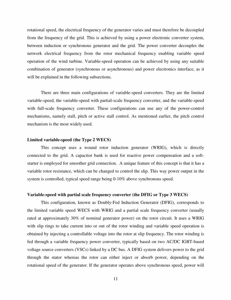
Variable-speed with partial scale frequency converter (the DFIG or Type 3 WECS)
This configuration, known as Doubly-Fed Induction Generator (DFIG), corresponds to
the limited variable speed WECS with WRIG and a partial scale frequency converter (usually
rated at approximately 30% of nominal generator power) on the rotor circuit. It uses a WRIG
with slip rings to take current into or out of the rotor winding and variable speed operation is
obtained by injecting a controllable voltage into the rotor at slip frequency. The rotor winding is
fed through a variable frequency power converter, typically based on two AC/DC IGBT-based
voltage source converters (VSCs) linked by a DC bus. A DFIG system delivers power to the grid
through the stator whereas the rotor can either inject or absorb power, depending on the
rotational speed of the generator. If the generator operates above synchronous speed, power will
Page 26
12
be delivered from the rotor through the converter to the network, and if the generator operates
below synchronous speed, the rotor will absorb power from the network through the converters.
The partial-scale frequency converter compensates for reactive power and provides a smoother
grid connection. It has a relatively wide range of dynamic speed control, typically 30% around
the synchronous speed. Its main drawbacks are the use of slip rings and high short-circuit
currents in the case of grid faults (as compared to the Type 4 WG – presented in the next
subsection). Thus in this system, it is possible to control both active and reactive power,
providing high grid performance. In addition, the power electronics converter enables the wind
turbine to act as a more dynamic power source to the grid.
Variable-speed with full-scale frequency converter (the Type 4 WECS)
This configuration corresponds to the full variable speed wind turbine, with the generator
connected to the grid through a full-scale frequency converter. The frequency converter
compensates for reactive power compensation and provides a smoother grid connection. The
generator is decoupled from the grid by a DC link. The power converter enables the system to
control active and reactive power very fast. The generator can be electrically excited (WRIG or
WRSG) or by a permanent magnet (PMSG). The gearbox may not be required in some
configurations using a direct driven multipole generator. Enercon, Made and Lagerway are well-
known manufacturers of this topology. The synchronous generators and full-scale converters
configuration is also referred to as Type 4 generators.
While DFIGs have gained popularity in recent years, Type 4 generators have been
gradually capturing the market [8]. As compared to the DFIGs, Type 4 WECSs have a wider
range for the controlled speed, are more efficient, less complicated, and easier to construct from
an electrical engineering perspective [8]-[12]. In addition, the Type 4 WECS can be made direct-
driven system without using a gear box, resulting in reduced noise, installation and maintenance
costs. SG can also be connected to diode rectifier or VSC. A major cost benefit is in using a
diode bridge rectifier [7]. The synchronous generators can be electrically excited or excited by
permanent magnets. The Permanent Magnet Synchronous Generators (PMSG) do not require
external excitation current, meaning less losses, improved efficiency and more compact size [7],
[13]. Further detailing of this topology is presented in the next section.
Page 27
13
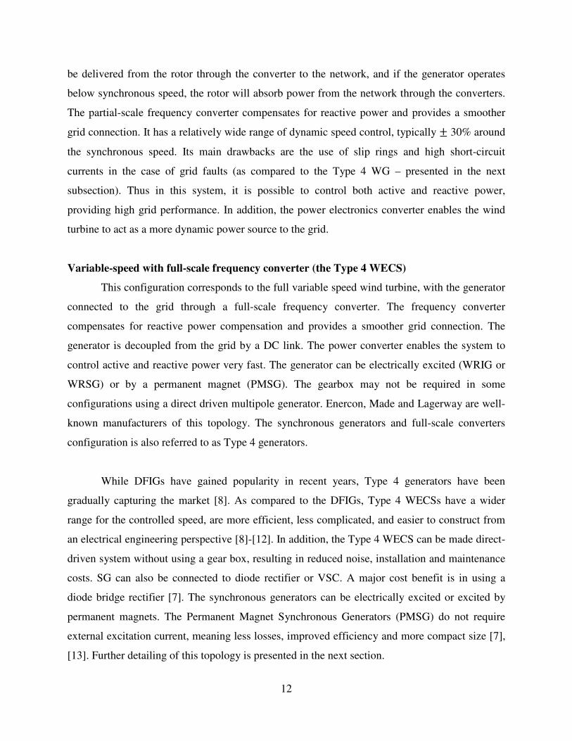
2.3 Synchronous Generator and Full-Scale Converter WECS
The topology of the Type 4 WECS is shown in Fig. 2.2.
Figure 2.2: Synchronous generator and full-scale converter WECS
2.3.1 Structure
As shown in Figure 2.2, the Type 4 WECS is composed of a synchronous generator, a
diode-bridge rectifier, a boost converter, and a Pulse-Width Modulation (PWM) Voltage Source
Inverter (VSI).
Generator
The generator can be magnetised electrically or by permanent magnets. Two types of
synchronous generators have often been used in the wind turbine industry: (1) the wound rotor
synchronous generator (WRSG) and (2) the permanent magnet synchronous generator (PMSG).
The wind turbine manufacturers Enercon, Lagerwey and Made apply the WRSG concept.
Examples of wind turbine manufacturers that use the configuration with PMSGs are Lagerwey,
WinWind and Multibrid. The synchronous generator with a suitable number of poles can be used
for direct-drive applications without any gearbox. PMSGs do not require external excitation
current, meaning less losses, improved efficiency and more compact size [7]-[13]. This is the
topology studied in this thesis.
PWind Pe Pdcr Pdc Po_abc
Wind
Turbine
Diode Bridge
Rectifier
Boost
Converter
PWM
Inverter
Grid
PMSG
+
Vdca
−
+
Vdci
−
Pm
Is
Idcr Idcb
Io_abc
Page 28
14
Converters
The topology used in this thesis applies an uncontrolled diode-bridge rectifier as the
generator-side converter. A DC booster is used to stabilize the DC link voltage whereas the
network-side inverter (PWM VSI) controls the operation of the generator. The PWM VSI can be
controlled using load-angle techniques or current controllers developed in a voltage-oriented dq
reference frame. Another existing topology applies a PMSG and a power converter system
consisting of two back-to-back voltage source converters.
Full-scale power converters ensure optimal wind energy conversion efficiency
throughout their operating range and enable the WECS to meet various grid codes. Power
converters are used to transfer power from the generator to the grid. The generator power is fed
via the stator windings into the suitable power converters, which convert a three-phase AC
voltage with variable frequency and magnitude into DC, and then convert the DC voltage into
AC with fixed frequency and magnitude for grid connection. However, the grid-side converter,
whose electric frequency and voltage are fixed to match those of the grid, can be set to control
the injection of reactive power and imposed voltage on the grid. The specific characteristics and
dynamics of the electrical generators are effectively isolated from the power network. Hence the
output of the generator system may vary as the wind speed changes, while the network frequency
remains unchanged, permitting variable speed operation. The power converter acts as an energy
buffer for the power fluctuations caused by the wind and for transients coming from the grid
side. Power converter can be arranged in various ways. While the generator-side converter
(GSC) can be a diode-based rectifier or a PWM voltage source converter, the network-side
converter (NSC) is typically a PWM source converter.
A DC inductor is used to smooth the ripple of the DC link. The small grid filter is used to
eliminate the high order harmonics. These are not shown in figure.
2.3.2 Operation
The working principle of this generator is as follows (refer to Figure 2.2). The wind
turbine axis is directly coupled to the generator rotor. Since the wind power fluctuates with the
Page 29
15
wind velocity, the PMSG output voltage and frequency vary continuously. The varying AC
voltage is rectified into DC by the diode bridge rectifier (Vdcr). The rectified DC voltage (Vdcr) is
boosted by the DC/DC boost converter by controlling its duty ratio to obtain a regulated voltage
(Vdca) across the capacitor. This DC voltage is inverted to obtain the desired AC voltage and
frequency by using the PWM VSI. The WECS can be operated under power factor control mode
to exchange only active power with the grid.
Page 30
16
Chapter 3
Proposed Model of the Type 4 PMSG WECS
The complete structure of a Type 4 PMSG WECS is modeled and validated in this
chapter. Section 3.1 presents the modeling technique and section 3.2 presents the validation of
the model.
3.1 Model
The complete model of the three-phase Type 4 WECS incorporates six sub-models: (1) a
Wind Turbine, (2) a Permanent Magnet Synchronous Generator, (3) a three-phase diode-bridge
rectifier, (4) a Boost Converter, (5) a Voltage Source Inverter, and (6) the control mode action.
Only the models at fundamental frequency are used in steady-state analysis of power
systems. These models represent AC fundamental frequency and DC average values of voltages
and currents [13]. The approach to develop models and equivalent circuit includes the balance of
power and inclusion of converter losses [30]-[31]. In converters, the conduction losses depend on
the on-state voltage, on-state resistance and current through it [32]. With the constant DC
voltage, the converter losses can be represented by a constant value [13]. This is done by the
drop across an equivalent series resistor which also includes the resistance of inductors [31].
Hence the equivalent circuit with a voltage source in series with impedance can be used for
inclusion in the power flow [34]. The equivalent circuit of the complete model is shown in
Figure 3.1.
Figure 3.1: Proposed equivalent model for the Type 4 WECS
Generator Boost
Converter Voltage Source Inv Rectifier
Ea
+
+ + +
-
Vt_a Rs
Rs
Rs
Xs
Xs
Xs
Rr Idcr
Vdcr
Rb Idcb
Vdcb Vdca -
Eb
Ec
"_ "_
Va_a
Va_b
Va_c
Vo_ab
Vo_bc - - -
Is_a
Is_b
Is_c
Vdci
Ro Xo
Ro Xo
Ro Xo
Io_a
Io_b
Io_c
Page 31
17
The six following sub-sections describe the models of each of the five components, and
the seventh sub-section presents the development of the proposed algorithm for obtaining the full
model of the Type 4 PMSG WECS.
3.1.1 Wind Turbine Model
The wind turbine extracts a portion of wind power (Pwind) from the swept area of the rotor
disc and converts it into mechanical power (%&) as determined below
%& ' 1 2⁄ . ,. -. ./0123 . 45 617
where ρ is the air density (approximately 1.225 kg/m3), A is the swept area of the rotor (m
2), and
ωwind is the free wind speed (m/s). The power coefficient (CP 8 0.593) can be maximized for a
given wind speed by optimally adjusting the values of tip speed ratio and the blade pitch angle
using data supplied by the manufacturer. In this thesis, through the optimal choice of CP for a
given wind speed, %& =>? .& (rotor mechanical speed) are assumed to be known and are used
as inputs to the synchronous generator.
3.1.2 Synchronous Generator Model
The induced EMFs (electromotive force) in the PMSG are considered sinusoidal [28] and
the saturation of magnetic core and the effect of saliency of the rotor are neglected [16]. In the
Type 4 PMSG WECS, the generator rotor shaft is directly coupled to the wind turbine such that
they have a mechanical speed of ωm.
The electrical speed (ωe), rotor mechanical speed (ωm), and the number of pair of poles (p) are
related as .@ ' A. .&. The PMSG is assumed balanced and its induced voltage in phase ph can
be expressed as
B5C ' 4.44. . E. FGHI 627
Page 32
18
where ϕ is magnetic flux which is a constant in a PMSG and N is the number of coil turns. This
value is known a priori in this work.
Therefore, the generator terminal voltage in phase ph is obtained as
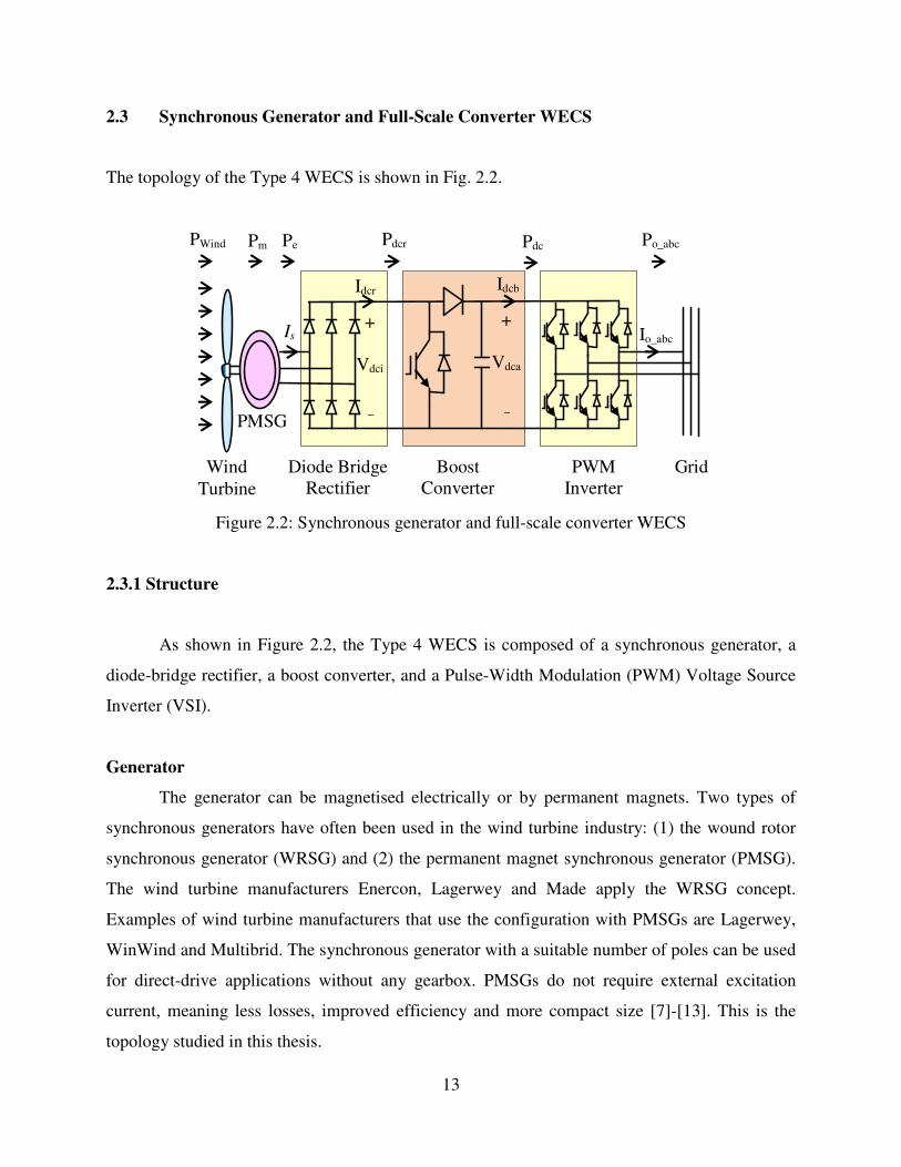
JK_5CLMK_5C ' B5CLMN_5C O PN_5CLQN_5C. 6RN S TUN7 637
where Rs is the winding resistance and Xs is the synchronous reactance. Also, MN_5C, MK_5C and
QN_5C are the phase angles of B"5C, J"K_5C and phase current P N_5C, respectively, for the phase ph.
This equation defines the steady-state characteristic of the generator and can be represented by
the corresponding equivalent circuit contained in Figure 3.1.
The generator’s input mechanical power can be calculated as
%& ' 3B5C. PN_5C . 4VW 6MNXY O QNXY7 647
3.1.3 Three Phase Diode Bridge Rectifier Model
Due to variations in wind speed, the generator output is of variable voltage and
frequency. In order to achieve controllable speed in the WECS application, the first step consists
of a three-phase diode-bridge rectifier being used to rectify the AC voltage into DC voltage. This
device is of simple design and low cost. Thus, as the commutation effect is neglected, the
generator output power factor is considered as unity. The rectifier output DC voltage is given by
J2Z[ ' 3 \⁄ . √6. JK_5C 657
The rectifier output DC current can be obtained as [35]
P2Z[ ' \ √6⁄ . PN_5C 667
Page 33
19
Finally, the terminal voltage of rectifier is given by
J2Z0 ' J2Z[ O R[ . P2Z[ 677
where R[ represents losses of the rectifier. The equivalent circuit used to represent the diode-
bridge rectifier is shown in Figure 3.1, which presents all major components of the Type 4
PMSG WECS. With the losses being represented in the series resistanceR[, the rectification
process is power invariant and therefore:
3 . JK_5C . PN_5C. 4VW `MK_5C O QN_5Ca ' J2Z[ . P2Z[ (8)
3.1.4 Boost Converter Model
The DC voltage across the boost converter is controlled to be approximately constant and
smooth by varying the duty cycle D in response to the variations in the input DC voltage. Thus it
stabilizes the voltage at the DC terminal of the inverter [35]. The controlled DC voltage across of
the boost converter is given by
J2Zb ' 161 O c7 J2Z0 697
while the DC current output from the boost converter is
P2Zb ' 61 O c7. P2Z[ 6107
Accounting for the Boost Converter losses in the series resistance Rb, the DC voltage output of
the boost converter is calculated as
J2Zd ' J2Zb O Rb . P2Zb 6117
Figure 3.1 shows the equivalent circuit used for the boost converter.
Page 34
20
3.1.5 Voltage Source Inverter
The connection of the WECS to the grid is done through a self commutated PWM VSI. A
filter is typically used to limit harmonics [35]. The line-to-neural voltage at the VSI terminal is
therefore
Jd_5C ' √32√2 . ed. J2Zd 6127
where ma is the modulation index that is bound as 0 ≤ ma ≤ 1.
The three-phase VSI output voltage is given by
Jf_5CLMf_5C ' Jd_5CLMd_5C. OPf_5CLQf_5C. 6Rf S T. Uf7 6137
The value of Rf is chosen as to include all losses associated in the in the VSI. With Rf
representing all losses, the conversion process is power invariant and hence,
3 Jd_5C. Pf_5C . 4VW `Md_5C O Qf_5Ca ' J2Zd P2Zb (14)
The power output from the VSI can be written as
%f_5C S T . gf_5C ' Jf_5CLMf_5C. `Pf_5CL Qf_5Cah 6157
The equivalent circuit used for the PWM VSI is shown in Figure 3.1.
3.1.6 Control Mode Action
The Type 4 WECS is modeled to operate under the power factor control mode such that
the output maintains a unity power factor. To represent the action of this control mode, at the bus
where the WECS is connected (Point of Common Coupling – PCC), the reactive power balance
equation is therefore given by
Page 35
21
i gf_5C5Cjd,b,Z
' 0 . 6167
3.1.7 Proposed Complete Type 4 PMSG WECS Model Algorithm
Subsections 3.1.1-3.1.6 were used to develop the models of the important elements of the
Type 4 PMSG WECS. The complete model was shown in Figure 3.1. The equations presented in
the previous sections used to represent the behaviour of the Type 4 generator are:
• Wind turbine: (1);
• Synchronous Generator Model: (2)-(4);
• Diode Bridge Rectifier: (5) - (8);
• Boost Converter: (9)-(11);
• Voltage Source Inverter: (12)-(15);
• Controller: (16)
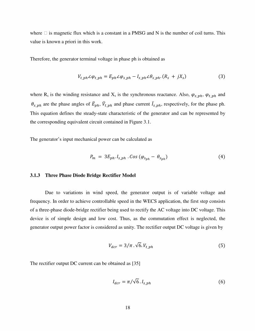
3.2 Validation
In this section, the developed model is validated by using time-domain simulation via the
Matlab-Simulink package. The Simulink diagram is shown in Figure 3.2. By using this model at
any given wind speed and bus bar voltage, the complete state of the Type 4 PMSG WECS can be
computed. During the validation process, the WECS is operated in the power factor control
mode.
Page 36
22
Figure 3.2: Type 4 WECS model in Matlab-Simulink
The results are tabulated in Table 3.1. The PMSG, Rectifier, Boost Converter and PMW
VSI data sets were used according to [37], and are presented in Appendix A. On solving the
same data set as that used by MATLAB-Simulink, virtually identical results were obtained.
Further, using hand calculations, the same results as those of the proposed model were obtained.
These results in Table 3.1 validate the proposed model.
Table 3.1: Results from both models for the Type 4 WECS
Parameter Matlab-Simulink Model Proposed Model
Pm (MW) 2.07711 2.07711
Vt_ph (Volt) 412.805 ∠0 412.805 ∠0
Pe (MW) 2.07468 2.07474
Vdcr (Volt) 910.2 910.2
Pdcr (MW) 2.04430 2.04428
Vdcb (Volt) 1100 1100
Pdcb (MW) 2.02686 2.02686
Vo_ph (Volt) 339.533 ∠0 339.533 ∠0
Po_abc (MW) 2.00589 2.00592
Note: The proposed model was also verified analytically.
Page 37
23
The Simulink model has been used for validation purposes only and it would have serious
limitations should it be used for load flow analysis because of computational time. For a simple
2-bus system, the Simulink model takes 10-20 times longer to compute than the proposed model
and for larger system this time difference will escalate.
Page 38
24
Chapter 4
New Load Flow Approach with the Proposed Type 4 WECS Model
There are many efficient and reliable load flow solution techniques, which have been
developed and widely used for power system operation, control and planning in the transmission
level. Most of the WECS units are being connected in distribution networks. Generally,
distribution systems are radial and have a high R/X ratio. Therefore distribution systems power
flow computation is different and the conventional Load Flow methods may fail to converge to a
solution. Moreover, most of the distribution systems are unbalanced because of single-phase,
two-phase and three-phase loads. Traditional load flow programs are designed to model only
balanced three-phase power systems. Therefore, the traditional power flow methods may not be
able to solve power flow problems of distribution systems in the presence of DGs. Recently,
various methods have been developed to carry out the analysis of balanced and unbalanced radial
distribution systems. A first category of methods is based on the modification of existing
methods such as the Newton-Raphson and Gauss-Seidel and the second category is based on
forward and/or backward sweep processes using Kirchoff’s Laws.
Forward/backward sweep-based algorithms are more popular because of their low
memory requirements, high computational efficiency and reliable convergence characteristic.
These methods take advantage of the radial nature of distribution networks where there is a
unique path from any given bus to the source.
In this chapter a new approach of load flow to which the proposed Type 4 PMSG WECS
model is integrated and presented. A comparison with the traditional fixed PQ model is also
presented.
4.1 Load Flow Method Description
There are many variants of Forward/backward sweep-based methods but the basic
algorithm is the same. The general algorithm consists of two basic steps, backward sweep and
Page 39
25
forward sweep, which are repeated until convergence is achieved. The backward sweep is
primarily a branch current or power flow summation with possible voltage updates, from the
receiving end to the sending end of the feeder and/or laterals. The forward sweep is primarily a
node voltage drop calculation with possible current or power flow updates. The load flow
technique based on the ladder network theory is used in this study [38].
A detailed explanation on the ladder iterative technique is presented in this section. The
flowchart presented in figure 4.1 presents the steps of the ladder-iterative technique power flow
algorithm.
Page 40
26
Start
Read input data &
Assume at WECS bus P = 01
4 Assume all Bus Voltages = 1pu
3 IT = 1
ERR =1
2 Model Series/Shunt feeder component
5 Compute Bus Currents
Stop
YES
WECS Model7
Not
Converged
NO
Back ward Sweep Calculation Determine voltage10
WECS Model11
NO
6 IT < 100
9 ERR < TOL
Voltage
Solution12
8Forward Sweep Calculation
Determine Current
Figure 4.1: Flowchart of Load Flow using conventional Ladder Iterative Technique
Page 41
27
Each step of this algorithm is presented in detail as follows.
Step 1: Read input data
The Matlab code including the algorithm to read the data is given in Appendix D. Initially at
WECS bus, power generation/consumption is considered as zero, i.e., Pabc = Qabc = 0.
Step 2: Modeling of Series Feeder Components
Different Series Feeder Components (SFC), such as lines, transformers, and etc, are modeled to
compute the generalized matrices a, b, c, d, A and B, which will be used in Step 8. This
modeling procedure is explained in Appendix C.
Step 3: Initialisation: assume IT = 1 and ERR =1
Step 4: Assume lbus = 1 pu at all buses
Voltage at all buses is assumed to be the same as the source voltage, i.e., = 1 p.u.
Step 5: Compute the bus currents
Bus load currents and thus bus currents at all buses, including the WECS bus, are computed
using the appropriate relations, depending on the type of load, as specified in Appendix B.
Step 6: While IT<100
The maximum number of iterations is specified (refer to algorithm in Appendix D).
Step 7: Integrate the WECS model
The Type 4 WECS model, as given in Appendix E, is integrated and values of system loads (P
and Q) are updated.
Page 42
28
Step 8: Forward Sweep Calculation
The current is determined during the Forward Sweep, starting from the last node and sweeping
every node until the first node (or source) is reached. After integrating the WECS model, bus
load currents and thus bus currents are updated, similarly to what was done in step 5. The line
current flowing from the last node to the first node is found. The voltage at the next bus and line
current in next section are updated by using this line current, the voltage at the previous node and
the a, b, c, d parameters obtained in Step 2.
The bus load currents and the bus currents are updated using updated bus voltages.
Step 9: Compute ERR and Check ERR<TOL
The error is computed by comparing the voltage found at the first bus in step 8 with the specified
voltage (i.e., 1 p.u.) at the first bus.
If this Error is more than the tolerance specified in the data file, then proceed with the Backward
sweep (Step 10); otherwise go to Step 12.
The processes of Forward sweep and Backward sweep continue until the error is smaller than the
specified tolerance value.
Step 10: Backward Sweep Calculation
During the Backward sweep, the voltage is determined, starting from the source node to the end
node.
The voltage at a node is determined using the specified voltage from the previous node, the
forward sweep bus current (Step 8) flowing between nodes, and the A & B parameters obtained
from the models of series components (Step 2).
In this way, the updated new voltages at all end nodes are computed.
Page 43
29
Step 11: IT = IT + 1
This completes the first iteration and the next iteration will start at Step 6. Now the forward
sweep calculation will start by using the new updated end voltages determined in the backward
sweep of the previous iteration.
Step 12: Solution:
The forward sweep and backward sweep calculations are continued until the calculated voltage
at the source or first node is smaller than the specified tolerance value, i.e., until ERR<TOL. At
this point the voltages at all nodes and current flowing in all components / segments are known.
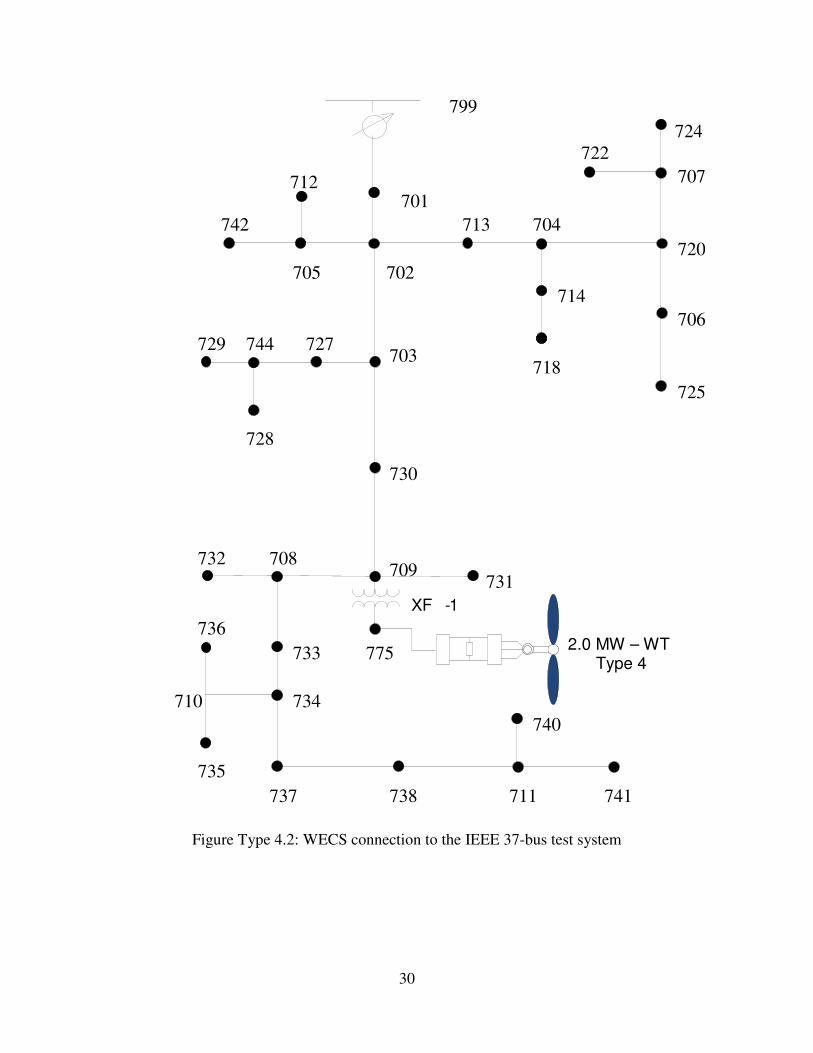
4.2 Test System Description
In this section, the unbalanced IEEE 37-bus test system (presented in [39]) is used to test
the proposed Type 4 WECS model. The proposed WG model was installed on bus # 775, as
shown in Figure 4.2.
Further changes were made into the original IEEE 37-bus system as follows:
1. The 2 MW rated Type 4 WG was connected to bus # 775.
2. According to the WG rating, the rating of the transformer XFM-1 was changed from 500
kVA to 2 MVA, and its low voltage side rating was changed from 480 V to 575V.
3. To clearly understand the effect of the WG model on the system, a 1.0 MW load was
added to each of the phases of buses # 730 and # 731. These additional loads make
voltage changes at the WG bus more pronounced.
Page 44
30
Figure Type 4.2: WECS connection to the IEEE 37-bus test system
799
701
742
705 702 720
704713
707
722
703744729
728
727
706
725
718
714
730
731709
708732
775733
736
734710
735 737 738 711 741
740
724
712
2.0 MW – WT Type 4
XF
-1
Page 45
31
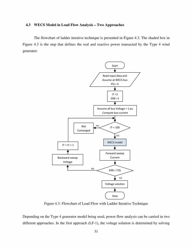
4.3 WECS Model in Load Flow Analysis – Two Approaches
The flowchart of ladder iterative technique is presented in Figure 4.3. The shaded box in
Figure 4.3 is the step that defines the real and reactive power transacted by the Type 4 wind
generator.
Figure 4.3: Flowchart of Load Flow with Ladder Iterative Technique
Depending on the Type 4 generator model being used, power flow analysis can be carried in two
different approaches. In the first approach (LF-1), the voltage solution is determined by solving
Read input data and
Assume at WECS bus
PQ = 0
Start
IT =1
ERR =1
Assume all bus Voltage = 1 pu
Compute bus current
IT < 100 NO Not
Converged
IT = IT + 1
YES
WECS model
Forward sweep
Current
NO ERR < TOL
Backward sweep
Voltage
YES
Voltage solution
Stop
Page 46
32
the power flow equations with the WECS represented as a fixed PQ load, i.e., P = Pa = Pb = Pc,
and Q = Qa = Qb = Qc are considered as input to the connection bus. This is the traditional
approach that has been widely adopted by industry. In the proposed approach (LF-2), the voltage
solution is determined by solving the power flow equations with the proposed WECS model as
presented in section 3.1.
4.3.1 Conventional Load Flow Method with the Conventional Type 4 WECS Model (LF-
1)
In this approach (LF-1), the Type 4 wind generator is represented as a fixed PQ load. To
represent the power factor control operating mode, the reactive power output of the Type 4
WECS was set to zero. For all iterations of the power flow algorithm (which was shown in
Figure 4.3), it was assumed that the Type 4 WECS generates fixed active power equal to Pabc = -
0.66832 MW in each of the phases, respectively. The results of this traditional method are shown
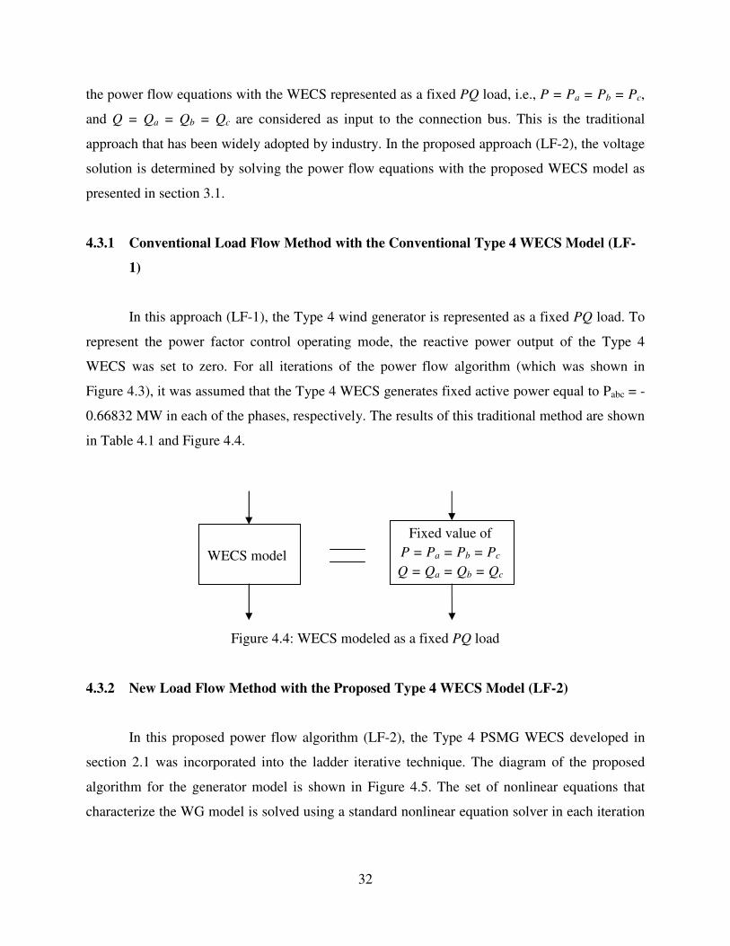
in Table 4.1 and Figure 4.4.
Figure 4.4: WECS modeled as a fixed PQ load
4.3.2 New Load Flow Method with the Proposed Type 4 WECS Model (LF-2)
In this proposed power flow algorithm (LF-2), the Type 4 PSMG WECS developed in
section 2.1 was incorporated into the ladder iterative technique. The diagram of the proposed
algorithm for the generator model is shown in Figure 4.5. The set of nonlinear equations that
characterize the WG model is solved using a standard nonlinear equation solver in each iteration
WECS model
Fixed value of
P = Pa = Pb = Pc
Q = Qa = Qb = Qc
Page 47
33
of the power flow algorithm. It computes the WG bus voltage computed in the preceding
iteration of the power flow algorithm.
In the first iteration of the ladder iterative technique, all bus voltages are assumed to be 1 p.u.
Therefore, the initial value of the PMSG WECS is also equal to Pa = Pb = Pc = -0.66832 MW and
reactive power is 0 MVAr on each phase. The resulting Pabc and Qabc act as a negative load bus
model for the next power flow iteration. In the following iterations, due to the presence of
unbalanced voltages, loads and system parameters, the PMSG WECS terminal voltage becomes
unbalanced and the PMSG WECS model yields unbalanced real power output values. The same
process will repeat until convergence. In each iterative step of the power flow algorithm, the
PMSG WECS model gives the actual value of currents, voltages, powers and losses on each
phase.
Figure 4.5: Proposed WECS model integrated in the Load Flow solution
4.3.3 Results and Comparison of the Power Flow Methods
The proposed Type 4 PMSG WECS model was integrated into the IEEE 37-bus
unbalanced test system for power flow studies. The voltage solutions of both power flow
approaches LF-1 (fixed PQ) and LF-2 (proposed WECS model) are presented in Table 4.1.
%& = f (./012) Normally
Va m Vb m Vcm 1 An
Wind Speed (./012) Bus Voltage
Pa , Qa Pb , Qb Pc , Qc
Solve proposed WECS Model
(1), (2)-(4), (5)-(8), (9)-(11), (12)-(15), (16)
Page 48
34
Table 4.1: Comparison of results from Load Flow methods for the IEEE 37-bus test system
Bus
Name
Phase a-b
Vab (pu)
Phase b-c
Vbc (pu)
Phase c-a
Vca (pu)
LF 1 LF 2 LF 1 LF 2 LF 1 LF 2
799 1.0000 1.0000 1.0000 1.0000 1.0000 1.0000
RG7 1.0437 1.0437 1.0250 1.0250 1.0345 1.0345
701 1.0193 1.0192 1.0022 1.0022 1.0033 1.0034
702 1.0029 1.0027 0.9883 0.9883 0.9846 0.9847
703 0.9831 0.9827 0.9732 0.9734 0.9640 0.9641
727 0.9819 0.9816 0.9726 0.9727 0.9630 0.9631
744 0.9812 0.9809 0.9722 0.9723 0.9625 0.9627
728 0.9808 0.9805 0.9718 0.9720 0.9621 0.9623
729 0.9809 0.9805 0.9721 0.9723 0.9624 0.9626
730 0.9627 0.9622 0.9564 0.9567 0.9440 0.9442
709 0.9600 0.9595 0.9546 0.9548 0.9416 0.9418
708 0.9575 0.9570 0.9535 0.9538 0.9393 0.9395
732 0.9574 0.9570 0.9534 0.9536 0.9388 0.9390
733 0.9551 0.9546 0.9525 0.9528 0.9373 0.9375
734 0.9517 0.9512 0.9510 0.9513 0.9339 0.9341
710 0.9512 0.9507 0.9500 0.9502 0.9323 0.9325
735 0.9511 0.9506 0.9498 0.9501 0.9318 0.9320
736 0.9506 0.9502 0.9484 0.9487 0.9320 0.9322
737 0.9483 0.9478 0.9500 0.9503 0.9317 0.9319
738 0.9471 0.9466 0.9496 0.9499 0.9306 0.9308
711 0.9468 0.9463 0.9494 0.9497 0.9296 0.9298
740 0.9467 0.9462 0.9493 0.9495 0.9291 0.9293
741 0.9468 0.9463 0.9494 0.9496 0.9293 0.9295
731 0.9479 0.9474 0.9429 0.9432 0.9299 0.9301
XF7 0.9600 0.9595 0.9546 0.9548 0.9416 0.9418
WECS 0.9599 0.9593 0.9551 0.9554 0.9419 0.9421
Page 49
35
705 1.0023 1.0020 0.9869 0.9870 0.9833 0.9834
712 1.0021 1.0019 0.9867 0.9868 0.9827 0.9828
742 1.0019 1.0017 0.9861 0.9862 0.9831 0.9832
713 1.0015 1.0013 0.9864 0.9865 0.9828 0.9829
704 0.9998 0.9996 0.9838 0.9839 0.9810 0.9811
714 0.9996 0.9994 0.9837 0.9838 0.9809 0.9810
718 0.9983 0.9980 0.9835 0.9836 0.9805 0.9806
720 0.9986 0.9984 0.9804 0.9805 0.9785 0.9786
706 0.9985 0.9983 0.9800 0.9801 0.9784 0.9785
725 0.9984 0.9982 0.9796 0.9797 0.9783 0.9784
707 0.9968 0.9966 0.9753 0.9754 0.9770 0.9771
722 0.9966 0.9964 0.9747 0.9748 0.9768 0.9769
724 0.9965 0.9963 0.9743 0.9744 0.9768 0.9769
LF-1: WG modeled as a Fixed PQ load LF-2: Proposed WG model
Figure 4.6 further quantifies the difference between the results from the two power flow
methods. Figure 4.6 shows that the difference between the line to line voltage (phases a-b)
solutions for both power flow methods is about 0.006 p.u. at the bus connecting the WECS and
nearby buses.
Figure 4.6: Comparison of line to line voltage a-b for both Load Flow approaches
0.9460
0.9480
0.9500
0.9520
0.9540
0.9560
0.9580
0.9600
79
9
70
1
70
3
74
4
72
9
70
9
73
2
73
4
73
5
73
7
71
1
74
1
XF
7
70
5
74
2
70
4
71
8
70
6
70
7
72
4
Vab
(p
.u.)
Bus Number
LF 1 - Fixed PQ
Approach
LF 2 - Proposed
Approach
Page 50
36
This comparison between the voltage solutions obtained by the two types of power flow
methods (LF-1 and LF-2) highlights the impact of the proposed active Type 4 PMSG WECS
model on each phase of the system. Significant differences in voltage and power on the generator
bus for both power flow methods can also be noticed and are summarized in Table 4.2.
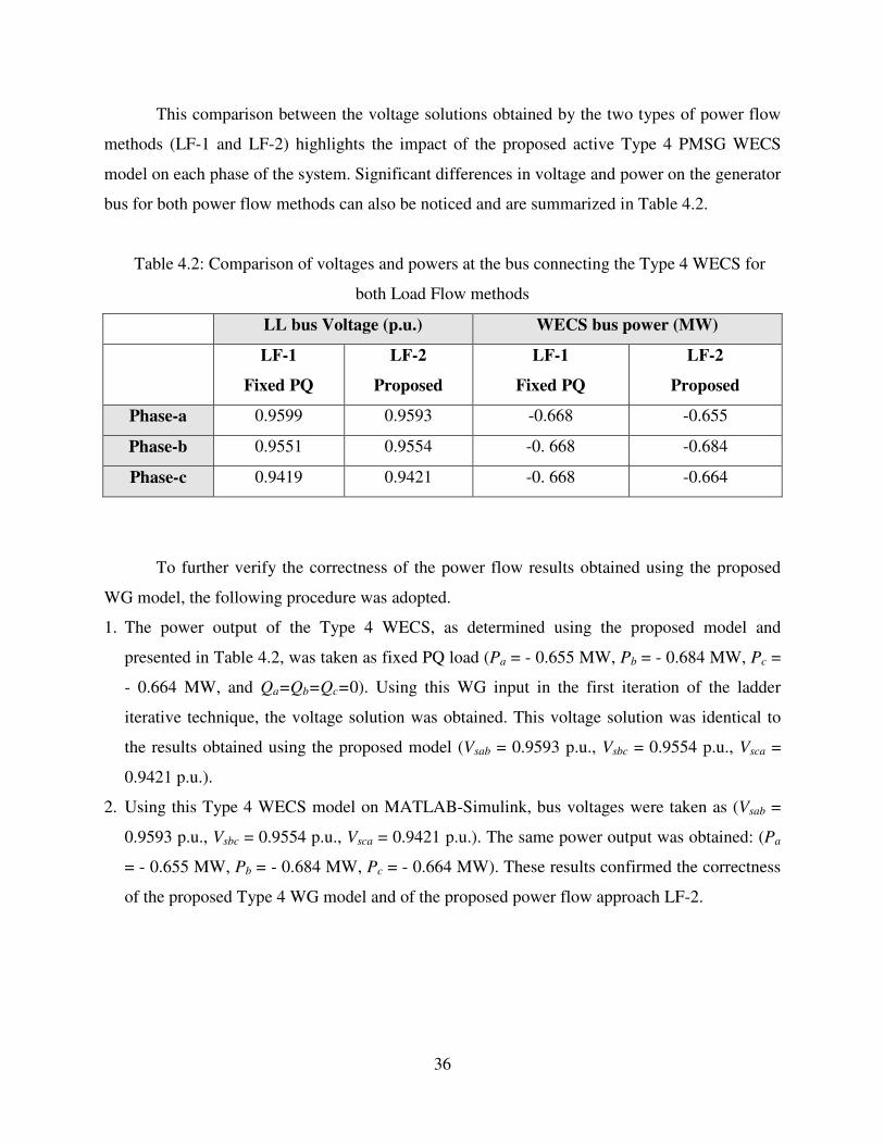
Table 4.2: Comparison of voltages and powers at the bus connecting the Type 4 WECS for
both Load Flow methods
LL bus Voltage (p.u.) WECS bus power (MW)
LF-1
Fixed PQ
LF-2
Proposed
LF-1
Fixed PQ
LF-2
Proposed
Phase-a 0.9599 0.9593 -0.668 -0.655
Phase-b 0.9551 0.9554 -0. 668 -0.684
Phase-c 0.9419 0.9421 -0. 668 -0.664
To further verify the correctness of the power flow results obtained using the proposed
WG model, the following procedure was adopted.
1. The power output of the Type 4 WECS, as determined using the proposed model and
presented in Table 4.2, was taken as fixed PQ load (Pa = - 0.655 MW, Pb = - 0.684 MW, Pc =
- 0.664 MW, and Qa=Qb=Qc=0). Using this WG input in the first iteration of the ladder
iterative technique, the voltage solution was obtained. This voltage solution was identical to
the results obtained using the proposed model (Vsab = 0.9593 p.u., Vsbc = 0.9554 p.u., Vsca =
0.9421 p.u.).
2. Using this Type 4 WECS model on MATLAB-Simulink, bus voltages were taken as (Vsab =
0.9593 p.u., Vsbc = 0.9554 p.u., Vsca = 0.9421 p.u.). The same power output was obtained: (Pa
= - 0.655 MW, Pb = - 0.684 MW, Pc = - 0.664 MW). These results confirmed the correctness
of the proposed Type 4 WG model and of the proposed power flow approach LF-2.
Page 51
37
Chapter 5
Conclusions and Suggestions for Future research
5.1 Conclusions
The Type 4 WECS (Synchronous Generator and Full-Scale Inverter) has gained popularity
and is capturing the market of wind generators. Traditionally, the Type 4 WG has been modeled
as a fixed negative PQ load in power flow studies. This fixed PQ model of a Type 4 WG leads to
inaccurate voltage solutions in power flow studies. With the widespread use of this technology of
wind generator in distribution systems, their accurate modeling is imperative, and is the focus of
this thesis. The main contributions of this research work can be summarized as follows:
1. This thesis has presented the development of an accurate three-phase model using a set of
nonlinear equations. The proposed model accounts for the synchronous generator, the
wind turbine, the three-phase diode bridge rectifier, the Boost converter, the PWM VSI,
and the Control Mode Action.
2. The proposed model was validated by comparing its results with those obtained from
MATLAB-Simulink and via analytical calculations. The proposed model takes much less
computational time than the Simulink model. For larger system, this time difference is
further increased.
3. The proposed model can be easily integrated into power flow algorithms. The integrated
power flow algorithm was presented and discussed.
4. Power Flow analysis results of an unbalanced three-phase IEEE 37-bus test system were
reported. The results obtained using the fixed PQ and the proposed models were
compared. The proposed model was once again validated using the 37-bus test system
and therefore shown to be accurate.
5. The proposed model creates an accurate three-phase representation of a Type 4 WG that
is suitable for power flow studies under unbalanced conditions. It is suitable for the
ladder iterative technique (as shown in this thesis) and equally suitable for Newton-
Raphson Technique as well.
Page 52
38
5.2 Suggestions for Future Research
The following are the suggestions for future research development.
• During this research work, the commutation effect in the synchronous-diode rectifier pair
was neglected. Further switching losses of converters were also neglected. Therefore, it is
possible to further modify the model by including these losses to obtain an even more
accurate model.
• A more detailed load flow analysis could also include models of other types of WECS
along with the Type 4 model. This would enable representing real distribution feeders
populated with a mix of different types of WECS.
Page 53
39
References
1. O. Anaya-Lara, N. Jenkins, J. Ekanayake, P. Cartwright, and M. Hughes , “Wind Energy
Generation: Modelling and Control ”, John Wiley & Sons Ltd, 2009.
2. F. Iov, M. Ciobotaru, and F. Blaabjerg, “Power Electronics Control of Wind Energy in
Distributed Power Systems.”
3. Z. Chen, “Wind turbine power converters: a comparative study,” Seventh International
Conference on Power Electronics and Variable Speed Drives, 1998, pp. 471-476.
4. Global Wind Energy Council, available online at http://www.gwec.net/index.php?id=97
5. Canadian Wind Energy Association, available online at
http://www.canwea.ca/media/index_e.php
6. T. Ackermann, “Wind Power in Power Systems”, John Wiley & Sons Ltd, 2005 pp. 64-
69.
7. J.A. Baroudi, V. Dinavahi, and A.M. Knight, “A review of power converter topologies
for wind generators,” Renewable Energy, vol. 32, 2007, pp. 2369-2385.
8. A.D. Hansen and L.H. Hansen, “Wind Turbine Concept Market Penetration over 10
Years (1995–2004),” Wind Energy, vol. 10, 2007, pp. 81-97.
9. H. Li and Z. Chen, “Overview of different wind generator systems and their
comparisons,” IET Renewable Power Generation Engineering and Technology, vol. 2,
2008, pp. 123-138.
10. A. Grauers, “Efficiency of three wind energy generator systems,” IEEE Transactions on
Energy Conversion, vol. 11, 1996, pp. 650-657.
11. A.D. Hansen and G. Michalke, “Modelling and Control of Variable -speed Multi-pole
Permanent Magnet Synchronous Generator Wind Turbine,” Wind Energy, vol. 11, 2008,
pp. 537-554.
12. L.M. Fernandez, C. a Garcia, and F. Jurado, “Operating capability as a PQ/PV node of a
direct-drive wind turbine based on a permanent magnet synchronous generator,”
Renewable Energy, vol. 35, Jun. 2010, pp. 1308-1318.
13. S. Achilles and M. Poller, “Direct Drive Synchronous Machine Models for Stability
Assessment of Wind Farms,” pp. 1-9. Available from,
http://www.digsilent.de/Consulting/Publications/DirectDrive_Modeling.pdf>.
Page 54
40
14. Y. Kazachkov, & R. Voelzke, “Modeling wind farms for power system load flow and
stability studies”. 2005 IEEE Russia Power Tech, pp. 1-8.
15. R. Ranjan, B. Venkatesh, A. Chaturvedi, and D. Das (2004) 'Power Flow Solution of
Three-Phase Unbalanced Radial Distribution Network', Electric Power Components and
Systems, vol. 32, no. 4, pp 421-433
16. A. E. Feijóo and J. Cidras, “Modeling of Wind Farms in the Load flow Analysis”, IEEE
Transactions on Power Systems, vol. 15, no. 1, Feb. 2000, pp. 110-115.
17. U. Eminoglu, “Modeling and application of wind turbine generating system (WTGS) to
distribution systems”, Renewable Energy, vol. 34, 2009, pp.2474-2483.
18. A. Feijóo, “On PQ Models for Asynchronous Wind Turbines”, IEEE Transactions on
Power Systems, vol. 24, No. 4, Nov. 2009, pp.1890-1891.
19. J. F. M. Padrón and A. E. Feijóo Lorenzo, “Calculating Steady-State Operating
Conditions for Doubly-Fed Induction Generator Wind Turbines”, IEEE Transactions on
Power Systems, vol. 25, no. 2, May 2010, pp. 922-928.
20. H. Chen, J. Chen, D. Shi, and X. Duan, “Power flow study and voltage stability analysis
for distribution systems with distributed generation,” 2006 IEEE Power Engineering
Society General Meeting, IEEE, 2006.
21. G. Coath and M. Al-Dabbagh, “Effect of Steady-State Wind Turbine Generator Models
on Power Flow Convergence and Voltage Stability Limit,” Australasian Universities
Power Engineering Conference, Hobart: 2005.
22. M. Ding, X. Guo, and Z. Zhang, “Three Phase Power Flow for Weakly Meshed
Distribution Network with Distributed Generation,” 2009 Asia-Pacific Power and Energy
Engineering Conference, 2009, pp. 1-7.
23. K. Divya and P. Rao, “Models for wind turbine generating systems and their application
in load flow studies,” Electric Power Systems Research, vol. 76, Jun. 2006, pp. 844-856.
24. S.M. Moghaddas-Tafreshi and E. Mashhour, “Distributed generation modeling for power
flow studies and a three-phase unbalanced power flow solution for radial distribution
systems considering distributed generation,” Electric Power Systems Research, vol. 79,
Apr. 2009, pp. 680-686.
25. M. Zhao, Z. Chen, and F. Blaabjerg, “Load flow analysis for variable speed offshore
wind farms,” IET Renewable Power Generation, vol. 3, 2009, pp. 120-132.
Page 55
41
26. F. Blaabjerg and Z. Chen, “Power Electronics for Modern Wind Turbines”, 1st ed.
Morgan & Claypool, 2006.
27. T. Burton, D. Sharpe, N. Jenkins, E. Bossanyi, “Wind Energy Hand Book”, John Wiley
& Sons, 2001, pp. 6-45.
28. Kundur P. Power System Stability and Control, EPRI. McGraw-Hill: New York, 1994.
pp.54.
29. An Introduction to Electrical Machines and Transformers - G. McPherson & R.D,
Laramore 2nd
ed. John Wiley & Sons-pp.47.
30. E. Muljadi, S. Drouilhet, R. Holz, and V. Gevorgian, “Analysis of permanent magnet
generator for wind power battery charging,” Thirty-First IAS Annual Meeting & Industry
Applications Conference, San Diego, CA: 1996, pp. 541-548.
31. A. de V. Jaén, E. Acha, and A.G. Expósito, “Voltage Source Converter Modeling for
Power System State Estimation: STATCOM and VSC-HVDC,” IEEE Transactions on
Power Systems, vol. 23, 2008, pp. 1552-1559.
32. K. Kretschmar and H.-P. Nee, “Analysis of the Efficiency and Suitability of Different
Converter Topologies for PM Integral Motors,” Proceedings of the Australian
Universities Power Engineering Conference, Perth, 2001, pp 519-525.
33. Angeles-Camacho, C., Tortelli, O., Acha, E., & Fuerte-Esquivel, C. (2003). Inclusion of a
high voltage DC-voltage source converter model in a Newton–Raphson power flow
algorithm. IEE Proceedings - Generation, Transmission and Distribution, vol. 150(6),
691-696.
34. F. Al Jowder and B.T. Ooi, “VSC-HVDC station with SSSC characteristics,” IEEE 34th
Annual Conference on Power Electronics Specialist. PESC ’03, 2003, pp. 1785-1791.
35. N. Mohan, T. M. Undeland, and W. P. Robbins, Power Electronics: Converters,
Applications and Design, 3rd ed. John Wiley & Sons, 2002.
36. C. Kim, V. K. Sood, G. Jang, S. Lim, and S. Lee, HVDC Transmission: Power
Conversion Applications in Power Systems,1st ed. John Wiley & Sons, 2009. pp. 329-
340.
37. The Mathworks Inc., “Simpower systemTM
5 Reference”, 2009, pp.2-17-2- 30, 2-881-2-
292.
Page 56
42
38. W. H. Kersting, “Distribution System Modeling and Analysis”, second edition, CRC
Press, 2007
39. IEEE PES, “Distribution Test feeders”,-37 bus feeder,
http://ewh.ieee.org/soc/pes/dsacom/testfeeders/index.html
Page 57
43
Appendix A
Data Set for the Type 4 PMSG WECS Model
Table A.1: Wind Turbine data set
Wind Turbine Nominal Power, Pn 2 MW
Nominal Wind Speed, .1 11 m/s
Grid Connection Voltage (LL) 575 V (RMS)
Table A.2: Generator data set
Nominal Power, Pn 2.22 MVA
Nominal frequency, fn 60 Hz
Nominal Voltage (LL),Vn 730 V(RMS)
Number of Pole-pairs, p 1
Stator Resistance, Rs 0.006 pu
Synchronous Reactance, Xs 1.305 pu
Table A.3: Converters data set
Rectifier Impedance 6.58 mΩ
Boost Converter Impedance 5.14 mΩ
Inverter Impedance 1.8 mΩ
Page 58
44
Appendix B
Load Models Description with General Equations
In distribution systems, loads can be wye (star) connected or delta connected and three-
phase, two-phase, or single-phase with unbalanced nature. These can be modeled as:
1. Constant real and reactive power (Constant PQ)
2. Constant current
3. Constant Impedance
4. Any combination of above.
Figure B.1 shows a generic delta connected load. In the IEEE-37 test feeder system, all loads are
delta connected. Therefore, only delta connected loads modeling is described here.
These load models are used in the iterative process of load-flow algorithm, where load voltages
are initially assumed.
For all loads, the line currents entering the load are required in order to perform the load-flow
analysis.
Figure B.1: Delta connected load
IBLb
IBLa
IBLc
a b
c
Sca
IBLca
Sbc
IBLbc
Sab
IBLab
Page 59
45
The general equations of current computations for each model are [38]:
Model
Computation of current
Constant PQ
(D-PQ)
(Type-001)
Popqq = rsttuttvh=
|stt||utt| ∠xqq O Qqq = |Popqq|∠yqq
The line to line voltages will change after each iteration and as a result the
new current magnitude and angles.
Constant I
(D-I)
(Type-002)
Magnitudes of currents are computed similarly to those in the constant PQ
model and held constant.
Meanwhile, the angle of the voltage changes after each iteration.
This keeps the power factor of the load constant.
Constant Z
(D-Z)
(Type-003)
Constant load impedance, zqq = |utt|
stth = |utt||stt| = |zqq|∠Qqq
The delta load IBL is a function of the constant load impedances and are
given by
Popqq = utt|tt =
|utt|||tt| ∠xqq O Qqq = |Popqq|∠yqq
VLL changes after each iteration until convergence is achieved.
Page 60
46
Appendix C
Computation of a, b, c, d, A, B Parameters of Series Feeder Components
The description of the test system includes the voltage regulator, transformer and line segments.
Therefore, the parameters a, b, c, d, A, B can be obtained by using the following equations [38]
and Matlab programming codes as described in Appendix D.
Voltage Regulator Transformer Line Segment
Open Delta type
(303)
Delta-Delta type
(404)
a =
aR 0 00 aR 0OaR OaR 0~
3 2 O1 O1O1 2 O1O1 O1 2 ~
1 0 00 1 00 0 1~ + rHv Z Y
b =
0
Z*n*rv*2 1 00 2 11 0 2~* 1 O1 01 2 0O2 O1 0~
Z
c =
0 0 Y r1 S rv Z Y v
d =
O
1aR 0 01aR 0 O 1aR0 0 1aR
1n 1 0 00 1 00 0 1~
a
A =
a
13 h n 2 O1 O1O1 2 O1O1 O1 2 ~
a/ 1 0 00 1 00 0 1~
B =
0
Z*rv*2 1 00 2 11 0 2~* 1 O1 01 2 0O2 O1 0~
A h Z
where
a = 1∠120°
aRa = 1-0.00625 * tpa
aRb = 1-0.00625 * tpb
aRc = 1-0.00625 * tpc
where
n = 1
where
Z and Y are line
section impedance and
admittance matrices
Page 61
47
Appendix D
MATLAB Code for Load Flow
Input Data File
4.8-volts-radial-37-node-system 2001 PEAK_LOAD 001 38 38 0001 1 4.8 4 26 1 35 0 0 0
1 1.0 0.001 2.5 1.05 0.95 100 MAIN no bn bnam p1-pd p2-qd p2-pd p2-qd p3-pd p3-qd type 1 1 B799 0.000 0.000 0.000 0.000 0.000 0.000 001 no bn bnam p1-pd p1-qd p2-pd p2-qd p3-pd p3-qd type 1 3 B701 0.140 0.070 0.140 0.070 0.350 0.175 001 2 14 B712 0.000 0.000 0.000 0.000 0.085 0.040 001 3 15 B713 0.000 0.000 0.000 0.000 0.085 0.040 001 4 16 B714 0.017 0.008 0.021 0.010 0.000 0.000 002 5 17 B718 0.085 0.040 0.000 0.000 0.000 0.000 003 6 18 B720 0.000 0.000 0.000 0.000 0.085 0.040 001 7 19 B722 0.000 0.000 0.140 0.070 0.021 0.010 002 8 20 B724 0.000 0.000 0.042 0.021 0.000 0.000 003 9 21 B725 0.000 0.000 0.042 0.021 0.000 0.000 001 10 22 B727 0.000 0.000 0.000 0.000 0.042 0.021 001 11 23 B728 0.042 0.021 0.042 0.021 0.042 0.021 001 12 24 B729 0.042 0.021 0.000 0.000 0.000 0.000 002 13 25 B730 1.000 0.000 1.000 0.000 1.085 0.040 003 14 26 B731 1.000 0.000 1.085 0.040 1.000 0.000 003 15 27 B732 0.000 0.000 0.000 0.000 0.042 0.021 001 16 28 B733 0.085 0.040 0.000 0.000 0.000 0.000 002 17 29 B734 0.000 0.000 0.000 0.000 0.042 0.021 001 18 30 B735 0.000 0.000 0.000 0.000 0.085 0.040 001 19 31 B736 0.000 0.000 0.042 0.021 0.000 0.000 003 20 32 B737 0.140 0.070 0.000 0.000 0.000 0.000 002 21 33 B738 0.126 0.062 0.000 0.000 0.000 0.000 001 22 34 B740 0.000 0.000 0.000 0.000 0.085 0.040 001 23 35 B741 0.000 0.000 0.000 0.000 0.042 0.021 002 24 36 B742 0.008 0.004 0.085 0.040 0.000 0.000 003 25 37 B744 0.042 0.021 0.000 0.000 0.000 0.000 001 26 38 B775 0.000 0.000 0.000 0.000 0.000 0.000 001 con dis diam nn c-dia con-GMR c-res s-diam str-GMR s-resis 721 0.5 1.98 20 1.150 0.03680 0.105 0.1019 0.00330 05.9026 722 0.5 1.56 16 0.813 0.02600 0.206 0.0808 0.00262 09.3747 723 0.5 1.10 07 0.414 0.01250 0.769 0.0641 0.00208 14.8722 724 0.5 0.98 06 0.292 0.00883 1.541 0.0641 0.00208 14.8722
Page 62
48
no fb tb tpa tpb tpc con 1 1 2 6.699843 3.902439024 0 303 no fb tb vllh vlll r x rat con 2 11 38 4.8 0.575 0.0009 0.0181 2.5 404 no fb tb lengt zer pos con 3 2 3 1.850 0.0 0.0 721 4 3 4 0.960 0.0 0.0 722 5 4 5 1.320 0.0 0.0 722 6 5 25 0.600 0.0 0.0 723 7 25 11 0.200 0.0 0.0 723 8 11 10 0.320 0.0 0.0 723 9 10 28 0.320 0.0 0.0 723 10 28 29 0.560 0.0 0.0 723 11 29 32 0.640 0.0 0.0 723 12 32 33 0.400 0.0 0.0 723 13 33 13 0.400 0.0 0.0 723 14 13 35 0.400 0.0 0.0 723 15 4 7 0.400 0.0 0.0 724 16 7 36 0.320 0.0 0.0 724 17 4 15 0.360 0.0 0.0 723 18 15 6 0.520 0.0 0.0 723 19 6 18 0.800 0.0 0.0 723 20 18 8 0.600 0.0 0.0 723 21 8 21 0.280 0.0 0.0 724 22 5 22 0.240 0.0 0.0 724 23 22 37 0.280 0.0 0.0 723 24 37 24 0.280 0.0 0.0 724 25 6 16 0.080 0.0 0.0 724 26 16 17 0.520 0.0 0.0 724 27 18 9 0.920 0.0 0.0 724 28 9 20 0.760 0.0 0.0 724 29 9 19 0.120 0.0 0.0 724 30 7 14 0.240 0.0 0.0 724 31 10 27 0.320 0.0 0.0 724 32 11 26 0.600 0.0 0.0 723 33 29 12 0.520 0.0 0.0 724 34 12 30 0.200 0.0 0.0 724 35 12 31 1.280 0.0 0.0 724 36 13 34 0.200 0.0 0.0 724 37 37 23 0.200 0.0 0.0 724 Main File to Read the Data and all Function Files
% File to read all data and function files function DATA global Z721 Z722 Z723 Z724 Y721 Y722 Y723 Y724 global LENGTH ZZERO ZPOSITIVE CONFIG global NB NBB NS NG NLB NTR NTRL NT NSHC NSVS NSHR NSH NREG global VSLACK TOLER PBASE VLMAX VLMIN ITMAX global BIND BSN BNAM PG QG PD1 QD1 PD2 QD2 PD3 QD3 LTP PDD1 QDD1 PDD2 QDD2
PDD3 QDD3 LTPD
Page 63
49
global TRNO FB TB VLLH VLLL R X PRAT global TPA TPB TPC global VBASE global ifp % input file pointers temp1 = input('Input File Name:' , 's' ); ifp = fopen(temp1,'r'); temp = fscanf(ifp,'%s',[1]); temp = fscanf(ifp,'%s',[1]); temp = fscanf(ifp,'%s',[1]); temp = fscanf(ifp,'%s',[1]); ttt = fscanf(ifp,'%d %d %d %d %f %d %d %d %d %d %d %d %d',[1,13]); % Reading
the following data NB = ttt(1); % Number of Buses NBB = ttt(2); NS = ttt(3); % Slack Bus Number NG = ttt(4); % Number of Generators VBASE = ttt(5); % Base Voltage in kV NCON = ttt(6); % Number of Line Configurations NLB = ttt(7); % Number of Load Buses NTR = ttt(8); % Number of Transformers NTRL = ttt(9); % Number of Transmission Lines NSHC = ttt(10); % Number of Shunt Capacitors NSVS = ttt(11); % Number of Switchable Capacitors NSHR = ttt(12); % Number of Shunt Reactors NREG = ttt(13); % Number of Regulators % Adding Components/Lines NT = NTR + NTRL+ NREG; % Number of Total Lines/Components NSH = NSHC + NSVS + NSHR; % Number of Shunts ttt = fscanf(ifp,'%f %f %f %f %f %d',[1,6]); % Reading the following data VSLACK = ttt(1); % Slack Bus Voltage TOLER = ttt(2); % Tolerance PBASE = ttt(3); % Base MVA VLMAX = ttt(4); % Maximum Load Bus Voltage VLMIN = ttt(5); % Minimum Load Bus Voltage ITMAX = ttt(6); % Maximum number of Iterations ttt = fscanf(ifp,'%s',[1]); % Reading the "Main" region % Initialising Matrix/Columns for Data BSN = zeros(NG+NLB,1); % Bus Serial Number BNAM = cell (NG+NLB); % Bus Name
Page 64
50
PDD1 = zeros(NG+NLB,1); QDD1 = zeros(NG+NLB,1); PDD2 = zeros(NG+NLB,1); QDD2 = zeros(NG+NLB,1); PDD3 = zeros(NG+NLB,1); QDD3 = zeros(NG+NLB,1); LTPD = zeros(NG+NLB,1); % Line Segment Data PD1 = zeros(NB,1); QD1 = zeros(NB,1); PD2 = zeros(NB,1); QD2 = zeros(NB,1); PD3 = zeros(NB,1); QD3 = zeros(NB,1); LTP = zeros(NB,1); % Reading Grid Supply Point BSNMAX=0; ttt = fscanf(ifp,'%s %s %s %s %s %s %s %s %s %s',[1,10]); for k = 1:NG ttt = fscanf(ifp,'%d %d',[1,2]); BSN(k) = ttt(2); ttt = fscanf(ifp,'%s',[1]); BNAM(k)= cellstr(ttt); ttt = fscanf(ifp,'%f %f %f %f %f %f %d',[1,7]); PDD1(k) = ttt(1); QDD1(k) = ttt(2); PDD2(k) = ttt(3); QDD2(k) = ttt(4); PDD3(k) = ttt(5); QDD3(k) = ttt(6); LTPD(k) = ttt(7); PDD1(k) = PDD1(k)/(PBASE/3); QDD1(k) = QDD1(k)/(PBASE/3); PDD2(k) = PDD2(k)/(PBASE/3); QDD2(k) = QDD2(k)/(PBASE/3); PDD3(k) = PDD3(k)/(PBASE/3); QDD3(k) = QDD3(k)/(PBASE/3); end %Reading Load Data ttt = fscanf(ifp,'%s %s %s %s %s %s %s %s %s %s',[1,10]); for k = NG+1:NG+NLB ttt = fscanf(ifp,'%d %d',[1,2]); BSN(k) = ttt(2); ttt = fscanf(ifp,'%s',[1]); BNAM(k)= cellstr(ttt); ttt = fscanf(ifp,'%f %f %f %f %f %f %d',[1,7]); PDD1(k) = ttt(1); QDD1(k) = ttt(2); PDD2(k) = ttt(3); QDD2(k) = ttt(4); PDD3(k) = ttt(5); QDD3(k) = ttt(6); LTPD(k) = ttt(7); PDD1(k) = PDD1(k)/(PBASE/3); QDD1(k) = QDD1(k)/(PBASE/3); PDD2(k) = PDD2(k)/(PBASE/3); QDD2(k) = QDD2(k)/(PBASE/3); PDD3(k) = PDD3(k)/(PBASE/3); QDD3(k) = QDD3(k)/(PBASE/3); end for i = 1:NG+NLB PD1(BSN(i),1) = PDD1(i,1); QD1(BSN(i),1) = QDD1(i,1); PD2(BSN(i),1) = PDD2(i,1); QD2(BSN(i),1) = QDD2(i,1); PD3(BSN(i),1) = PDD3(i,1); QD3(BSN(i),1) = QDD3(i,1); PD3(BSN(i),1) = PDD3(i,1); LTP(BSN(i),1) = LTPD(i,1); end BIND = zeros(NB,1); for k = 1:NB BIND(k) = k; end ttt = fscanf(ifp,'%s %s %s %s %s %s %s %s %s %s',[1,10]);
Page 65
51
%Reading Line Configarations for k=1:NCON ttt = fscanf(ifp,'%d %f %f %d %f %f %f %f %f %f',[1,10]); CONF(k) = ttt(1); switch CONF(k) case 721 [Z721 Y721]= CABLEZY(ttt(2), ttt(3), ttt(4), ttt(5), ttt(6),
ttt(7), ttt(8), ttt(9), ttt(10)); case 722 [Z722 Y722]= CABLEZY(ttt(2), ttt(3), ttt(4), ttt(5), ttt(6),
ttt(7), ttt(8), ttt(9), ttt(10)); case 723 [Z723 Y723]= CABLEZY(ttt(2), ttt(3), ttt(4), ttt(5), ttt(6),
ttt(7), ttt(8), ttt(9), ttt(10)); case 724 [Z724 Y724]= CABLEZY(ttt(2), ttt(3), ttt(4), ttt(5), ttt(6),
ttt(7), ttt(8), ttt(9), ttt(10)); end end TRNO = zeros(NT,1); FB = zeros(NT,1); TB = zeros(NT,1); LENGTH = zeros(NT,1); ZZERO = zeros(NT,1); ZPOSITIVE = zeros(NT,1); CONFIG = zeros(NT,1); ttt = fscanf(ifp,'%s %s %s %s %s %s %s',[1,7]); % Reading Voltage Regulator Data for k=1:NREG ttt = fscanf(ifp,'%d %d %d %f %f %f %d',[1,7]); VRNO(k) = ttt(1); FB(k)= ttt(2); TB(k)= ttt(3); TPA(k) = ttt(4); TPB(k) = ttt(5); TPC(k) = ttt(6); CONFIG(k)= ttt(7); end % Reading Transformer Data ttt = fscanf(ifp,'%s %s %s %s %s %s %s %s %s',[1,9]); for k=NREG+1:NREG+NTR ttt = fscanf(ifp,'%d %d %d %f %f %f %f %f %d',[1,9]); TRNO(k) = ttt(1); FB(k) = ttt(2); TB(k) = ttt(3); VLLH(k) = ttt(4); VLLL(k) = ttt(5); R(k) = ttt(6); X(k) = ttt(7); PRAT(k)=ttt(8); CONFIG(k)= ttt(9); R(k) = R(k)*(PBASE/PRAT(k))*((VLLH(k)/VBASE)^2); X(k) = X(k)*(PBASE/PRAT(k))*((VLLH(k)/VBASE)^2); end
Page 66
52
% Reading Transmission Line Data ttt = fscanf(ifp,'%s %s %s %s %s %s %s',[1,7]); for k=NREG+NTR+1:NT ttt = fscanf(ifp,'%d %d %d %f %f %f %d',[1,7]); TRNO(k) = ttt(1); FB(k) = ttt(2); TB(k) = ttt(3); LENGTH(k)= ttt(4); ZZERO(k)= ttt(5); ZPOSITIVE(k)= ttt(6); CONFIG(k)= ttt(7); end DATASTR; % Reading Data Structure Function File PFLOW_DS_SG; Function to Compute Line Impedance and Admittance matrices
function [ZABC, YABC] = CABLEZY(D, DOD, NN, DC, GMRC, RC, DS, GMRS, RS) R = (DOD-DS)/24; GMRN = (GMRS*NN*(R)^(NN-1))^(1/NN); RN = RS/NN; D1 = (D^(NN)-R^(NN))^(1/NN); D2 = ((2*D)^(NN)-R^(NN))^(1/NN); D3 = R; GMRD = [GMRC D1 D2 D3 D1 D2; D1 GMRC D1 D1 D3 D1;... D2 D1 GMRC D2 D1 D3; D3 D1 D2 GMRN D1 D2;... D1 D3 D1 D1 GMRN D1; D2 D1 D3 D2 D1 GMRN;]; ZABC = zeros(3,3); YABC = zeros(3,3); Z1 = zeros(3,3); Z2 = zeros(3,3); Z3 = zeros(3,3); Z4 = zeros(3,3); for i = 1:3 for j=1:3 if i == j Z1(i,i) =
complex((RC+0.09530),(0.12134*(log(1/GMRD(i,i))+7.93402))); Z2(i,i) =
complex((0.09530),(0.12134*(log(1/GMRD(i+3,i))+7.93402))); Z3(i,i) =
complex((0.09530),(0.12134*(log(1/GMRD(i,i+3))+7.93402))); Z4(i,i) =
complex((RN+0.09530),(0.12134*(log(1/GMRD(i+3,i+3))+7.93402))); else Z1(i,j) =
complex((0.09530),(0.12134*(log(1/GMRD(i,j))+7.93402))); Z2(i,j) =
complex((0.09530),(0.12134*(log(1/GMRD(i+3,j))+7.93402))); Z3(i,j) =
complex((0.09530),(0.12134*(log(1/GMRD(i,j+3))+7.93402)));
Page 67
53
Z4(i,j) =
complex((0.09530),(0.12134*(log(1/GMRD(i+3,j+3))+7.93402))); end YABC(i,i) = 0.000001*complex(0,77.3619/(log((R*12)/(DC/2))-
(1/NN)*log((NN*DS/2)/(R*12)))); end end ZABC = Z1-Z2*(Z4\eye(3))*Z3; end
Function to Compute a, b, c, d, A, B parameters of Line
function [a, b, c, d, A, B]=TLabcdAB(ZL, YG)
a= eye(3)+0.5*ZL*YG; b= ZL; c= YG+0.25*YG*ZL*YG; d= eye(3)+0.5*YG*ZL; A= a\eye(3); B= A*ZL;
Function to Compute a, b, c, d, A, B parameters of Transformer
function [a, b, c, d, A, B] = TRabcdAB(PBASE, vllh, vlll, r, x, con) a = zeros(3,3); b = zeros(3,3); c = zeros(3,3); d = zeros(3,3); A = zeros(3,3); B = zeros(3,3); zt= complex(r,x); W = (1/3)*[2 1 0;0 2 1; 1 0 2]; %Delta grounded wye if con == 401 nt = sqrt(3); a = (-nt/3)*[0 2 1; 1 0 2; 2 1 0]; b = a*zt*eye(3); c = zeros(3,3); d = (1/nt)*[1 -1 0; 0 1 -1; -1 0 1]; A = (1/nt)*[1 0 -1;-1 1 0;0 -1 1]; B = zt*eye(3); end %ungrounded wye delta if con == 402 nt = (1/sqrt(3)); a = nt*[0 -1 0; 0 1 -1; -1 0 1]; b = (nt/3)*zt*[1 -1 0; 1 2 0; -2 -1 0]; c = zeros(3,3); d = (1/(3*nt))*[1 -1 0; 1 2 0; -2 -1 0]; A = (1/(3*nt))*[2 1 0;0 2 1;1 0 2]; B = (1/3)*zt*[1 0 0; 0 1 0; -1 -1 0]; end
Page 68
54
%grounded wye grounded wye if con == 403 nt= 1; a = nt*eye(3); b = zt*a; c = zeros(3,3); d = (1/nt)*eye(3); A = d; B = zt*eye(3); end %delta delta if con == 404 nt = 1; a = (nt/3)*[2 -1 -1;-1 2 -1;-1 -1 2]; b = nt*zt*(1/9)*[2 1 0; 0 2 1; 1 0 2]*[1 -1 0; 1 2 0; -2 -1 0]; c = zeros(3,3); d = (1/nt)*eye(3); A = (1/(3*nt))*[2 -1 -1;-1 2 -1;-1 -1 2]; B = zt*(1/9)*[2 1 0; 0 2 1; 1 0 2]*[1 -1 0; 1 2 0; -2 -1 0]; end %Open wye open delta if con == 405 nt = sqrt(3); a = nt*[1 -1 0; 0 1 -1;0 0 0]; b = nt*zt*[1 0 0; 0 0 -1;0 0 0]; c = zeros(3,3); d = (1/nt)*[1 0 0; 0 0 -1;0 0 0]; A = (1/(3*nt))*[2 -1 0;-1 1 0;-1 -2 0]; B = (zt/3)*[2 0 -1; -1 0 -1; -1 0 -2]; end
Function to Compute a, b, c, d, A, B parameters of Voltage Regulator
function [a b c d A B] = VRabcdAB(tpa, tpb, tpc, con) a = zeros(3,3); b = zeros(3,3); c = zeros(3,3); d = zeros(3,3); A = zeros(3,3); B = zeros(3,3); W = (1/3)*[2 1 0;0 2 1; 1 0 2]; aRa = 1-0.00625*tpa; aRb = 1-0.00625*tpb; aRc = 1-0.00625*tpc; %Wye if con == 301 a = [aRa 0 0; 0 aRb 0; 0 0 aRc]; b = zeros(3,3); c = zeros(3,3); d = [1/aRa 0 0; 0 1/aRb 0; 0 0 1/aRc]; A = inv(a); B = zeros(3,3); end
Page 69
55
%Delta if con == 302 a = [aRa 1-aRb 0; 0 aRb 1-aRc; 1-aRa 0 aRc]; b = zeros(3,3); c = zeros(3,3); d = [aRa 0 1-aRc; 1-aRa aRb 0; 0 1-aRb aRc]; A = inv(a); B = zeros(3,3); end %Open delta if con == 303 a = [aRa 0 0; 0 aRb 0; -aRa -aRb 0]; a = W*a*(W^(-1)); b = zeros(3,3); c = zeros(3,3); d = [1/aRa 0 0; -1/aRa 0 -1/aRb; 0 0 1/aRb]; d = W*d*(W^(-1)); A = [1/aRa 0 0; 0 1/aRb 0; -1/aRa -1/aRb 0]; A = W*A*(W^(-1)); B = zeros(3,3); end
Ladder iterative Algorithm for Load Flow
function PFLOW_DS_SG global Z721 Z722 Z723 Z724 Y721 Y722 Y723 Y724 global NB NS NT global ZL global LENGTH CONFIG PBASE global a b c d A B V1 V2 I2 VLL VLN IB IBL AIBL ZB m n index enode enode2
enode3 enode4 line IE VBASE IL global PD1 QD1 PD2 QD2 PD3 QD3 LTP VLLH VLLL R X TOLER W D err_E E IP PG VP global CON TPA TPB TPC VF IF IT %% Initialise I and V : IBL= zeros(NB,3); % Load current at the bus AIBL= zeros(NB,3); IB= zeros(NB,3); % Incomming acurrent to the bus ZB = zeros(NB,3); VLN = zeros(NB,3); % Phase voltage VLL = zeros(NB,3); % Line to line voltage IP = zeros(NB,3); VP = zeros(NB,3); [m,n] = size(CON); D = [1 -1 0; 0 1 -1; -1 0 1]; W = (1/3)*[2 1 0;0 2 1; 1 0 2];
%% Step-3 Error E=1; IT=1 %% for i = 1:NB %% Step-4 VLN(i,1:3) = [1, 1*complex(-0.5,-0.866025), 1*complex(-0.5,0.866025)] ; VLL(i,1:3) = (W^(-1))*(VLN(i,:).');
Page 70
56
%% Step-5 switch LTP(i) case 001 % D-PQ Type Load IBL(i,1:3)=[conj(complex(PD1(i),QD1(i))/VLL(i,1))-
conj(complex(PD3(i),QD3(i))/VLL(i,3))... conj(complex(PD2(i),QD2(i))/VLL(i,2))-
conj(complex(PD1(i),QD1(i))/VLL(i,1)).... conj(complex(PD3(i),QD3(i))/VLL(i,3))-
conj(complex(PD2(i),QD2(i))/VLL(i,2))]; case 002 % D-I Type Load IBL(i,1:3)=[conj(complex(PD1(i),QD1(i))/VLL(i,1))-
conj(complex(PD3(i),QD3(i))/VLL(i,3))... conj(complex(PD2(i),QD2(i))/VLL(i,2))-
conj(complex(PD1(i),QD1(i))/VLL(i,1)).... conj(complex(PD3(i),QD3(i))/VLL(i,3))-
conj(complex(PD2(i),QD2(i))/VLL(i,2))]; AIBL(i,1:3)= [abs(IBL(i,1)) abs(IBL(i,2)) abs(IBL(i,3))]; case 003 % D-Z Type Load ZB(i,1:3)=[abs((VLL(i,1)))^2/conj(complex(PD1(i),QD1(i)))... abs((VLL(i,2)))^2/conj(complex(PD2(i),QD2(i))).... abs((VLL(i,3)))^2/conj(complex(PD3(i),QD3(i)))]; IBL(i,1:3)=[VLL(i,1)/ZB(i,1)-VLL(i,3)/ZB(i,3)... VLL(i,2)/ZB(i,2)-VLL(i,1)/ZB(i,1).... VLL(i,3)/ZB(i,3)-VLL(i,2)/ZB(i,2)]; case 011 % Y - PQ Load IBL(i,1:3)=[conj(sqrt(3)*complex(PD1(i),QD1(i))/VLL(i,1))... conj(sqrt(3)*complex(PD2(i),QD2(i))/VLL(i,2)).... conj(sqrt(3)*complex(PD3(i),QD3(i))/VLL(i,3))]; case 012 % Y - I Type Load IBL(i,1:3)=[conj(sqrt(3)*complex(PD1(i),QD1(i))/VLL(i,1))... conj(sqrt(3)*complex(PD2(i),QD2(i))/VLL(i,2)).... conj(sqrt(3)*complex(PD3(i),QD3(i))/VLL(i,3))]; AIBL(i,1:3) = [abs(IBL(i,1)) abs(IBL(i,2)) abs(IBL(i,3))]; case 013 % Y - Z Type Load
ZB(i,1:3)=[abs(VLL(i,1)/sqrt(3))^2/conj(complex(PD1(i),QD1(i)))...
abs(VLL(i,2)/sqrt(3))^2/conj(complex(PD2(i),QD2(i))).... abs(VLL(i,3)/sqrt(3))^2/conj(complex(PD3(i),QD3(i)))]; IBL(i,1:3)=[VLL(i,1)/(sqrt(3)*ZB(i,1))... VLL(i,2)/(sqrt(3)*ZB(i,2)).... VLL(i,3)/(sqrt(3)*ZB(i,3))]; end end IB=IBL ; %% Step-6 FORWARD SWEEP while IT<100 && abs(E) > TOLER*1 IL= zeros(NT,3); IE= zeros(NT,1); V2= zeros(3,3); I2= zeros(3,3); PG =
zeros(NB,3); enode = 0;
Page 71
57
%% Step-7 % % For LF=1 @1 pu % PD1(38)= -0.801984 ; PD2(38)= -0.801984 ; PD3(38)= -0.801984 ; % QD1(38)= 0 ; QD2(38)= 0 ; QD3(38)= 0 ; % For LF-2 [PD1(i) PD2(i) PD3(i) QD1(i) QD2(i) QD3(i)] =
wesfn(VLN(i,1),VLN(i,2),VLN(i,3)); % % For LF-3 % PD1(38)= -0.7832 ; PD2(38)= -0.8236 ; PD3(38)= -0.7955 ; % QD1(38)= 0 ; QD2(38)= 0 ; QD3(38)= 0 ; %% Step-8 for i = 1:NB %% Step-8A if CON(i,1)== 0 % branch end = 0 enode = i; % enode = receiving end specific bus
number. switch LTP(enode) % Update loads case 001
IBL(enode,1:3)=[conj(complex(PD1(enode),QD1(enode))/VLL(enode,1))-
conj(complex(PD3(enode),QD3(enode))/VLL(enode,3))...
conj(complex(PD2(enode),QD2(enode))/VLL(enode,2))-
conj(complex(PD1(enode),QD1(enode))/VLL(enode,1))....
conj(complex(PD3(enode),QD3(enode))/VLL(enode,3))-
conj(complex(PD2(enode),QD2(enode))/VLL(enode,2))]; case 002
IBL(enode,1:3)=[conj(complex(PD1(enode),QD1(enode))/VLL(enode,1))-
conj(complex(PD3(enode),QD3(enode))/VLL(enode,3))...
conj(complex(PD2(enode),QD2(enode))/VLL(enode,2))-
conj(complex(PD1(enode),QD1(enode))/VLL(enode,1))....
conj(complex(PD3(enode),QD3(enode))/VLL(enode,3))-
conj(complex(PD2(enode),QD2(enode))/VLL(enode,2))];
IBL(enode,1:3)=[AIBL(enode,1)*complex(cos(angle(IBL(enode,1))),sin(angle(IBL(
enode,1))))...
AIBL(enode,2)*complex(cos(angle(IBL(enode,2))),sin(angle(IBL(enode,2))))....
AIBL(enode,3)*complex(cos(angle(IBL(enode,3))),sin(angle(IBL(enode,3))))]; case 003 IBL(enode,1:3)=[VLL(enode,1)/ZB(enode,1)-
VLL(enode,3)/ZB(enode,3)...
Page 72
58
VLL(enode,2)/ZB(enode,2)-
VLL(enode,1)/ZB(enode,1).... VLL(enode,3)/ZB(enode,3)-
VLL(enode,2)/ZB(enode,2)] ; case 011
IBL(enode,1:3)=[conj(sqrt(3)*complex(PD1(enode),QD1(enode))/VLL(enode,1))...
conj(sqrt(3)*complex(PD2(enode),QD2(enode))/VLL(enode,2))....
conj(sqrt(3)*complex(PD3(enode),QD3(enode))/VLL(enode,3))] ; case 012
IBL(enode,1:3)=[conj(sqrt(3)*complex(PD1(enode),QD1(enode))/VLL(enode,1))...
conj(sqrt(3)*complex(PD2(enode),QD2(enode))/VLL(enode,2))....
conj(sqrt(3)*complex(PD3(enode),QD3(enode))/VLL(enode,3))];
IBL(enode,1:3)=[AIBL(enode,1)*complex(cos(angle(IBL(enode,1))),sin(angle(IBL(
enode,1))))...
AIBL(enode,2)*complex(cos(angle(IBL(enode,2))),sin(angle(IBL(enode,2))))....
AIBL(enode,3)*complex(cos(angle(IBL(enode,3))),sin(angle(IBL(enode,3))))] ; case 013
IBL(enode,1:3)=[VLL(enode,1)/(sqrt(3)*ZB(enode,1))...
VLL(enode,2)/(sqrt(3)*ZB(enode,2))....
VLL(enode,3)/(sqrt(3)*ZB(enode,3))]; end IB(enode,1:3)= IBL(enode,1:3); end %% Step-8B while enode > 0 for k=1:(n-1)/2 % k = 1:3 , n=7 for j=1:NB if CON(j,2*k+1)== enode enode2 = j ; line = CON(j,2*k); end end end switch CONFIG(line) case 721 ZL =
LENGTH(line)*(1/5.28)*Z721/(VBASE^2/PBASE); YG =
LENGTH(line)*(1/5.28)*Y721*(VBASE^2/PBASE); [a b c d A B]= TLabcdAB(ZL,YG); case 722
Page 73
59
ZL =
LENGTH(line)*(1/5.28)*Z722/(VBASE^2/PBASE); YG =
LENGTH(line)*(1/5.28)*Y722*(VBASE^2/PBASE); [a b c d A B]= TLabcdAB(ZL,YG); case 723 ZL =
LENGTH(line)*(1/5.28)*Z723/(VBASE^2/PBASE); YG =
LENGTH(line)*(1/5.28)*Y723*(VBASE^2/PBASE); [a b c d A B]= TLabcdAB(ZL,YG); case 724 ZL =
LENGTH(line)*(1/5.28)*Z724/(VBASE^2/PBASE); YG =
LENGTH(line)*(1/5.28)*Y724*(VBASE^2/PBASE); [a b c d A B]= TLabcdAB(ZL,YG); case 303 [a b c d A B]= VRabcdAB(TPA(line),
TPB(line), TPC(line), CONFIG(line)); case 404 [a b c d A B]= TRabcdAB(PBASE,
VLLH(line), VLLL(line), R(line), X(line), CONFIG(line)); otherwise ZL = LENGTH(line)*(1/5.28)*
Z(CONFIG(line))/(VBASE^2/PBASE); % Zpu = Zactual/Zbase YG = LENGTH(line)*(1/5.28)*
Y(CONFIG(line))*(VBASE^2/PBASE); [a b c d A B]= TLabcdAB(ZL,YG) ; end V2 = a*[VLN(enode,1); VLN(enode,2); VLN(enode,3);] +
b*[IB(enode,1); IB(enode,2); IB(enode,3);] ; % enode = receiving end bus no. I2 = c*[VLN(enode,1); VLN(enode,2); VLN(enode,3);] +
d*[IB(enode,1); IB(enode,2); IB(enode,3);] ; IL(line,1:3)= I2 ; IE(line,1) = 1 ; VLN(enode2,1:3)= V2; VLL(enode2,1:3)= ((W^(-1))*[VLN(enode2,1);
VLN(enode2,2); VLN(enode2,3)]).' ; % VLN to VLL convert %% Step-8C switch LTP(enode2) % Update loads case 001
IBL(enode2,1:3)=[conj(complex(PD1(enode2),QD1(enode2))/VLL(enode2,1))-
conj(complex(PD3(enode2),QD3(enode2))/VLL(enode2,3))... conj(complex(PD2(enode2),QD2(enode2))/VLL(enode2,2))-
conj(complex(PD1(enode2),QD1(enode2))/VLL(enode2,1))....
conj(complex(PD3(enode2),QD3(enode2))/VLL(enode2,3))-
conj(complex(PD2(enode2),QD2(enode2))/VLL(enode2,2))];
Page 74
60
case 002
IBL(enode2,1:3)=[conj(complex(PD1(enode2),QD1(enode2))/VLL(enode2,1))-
conj(complex(PD3(enode2),QD3(enode2))/VLL(enode2,3))...
conj(complex(PD2(enode2),QD2(enode2))/VLL(enode2,2))-
conj(complex(PD1(enode2),QD1(enode2))/VLL(enode2,1))....
conj(complex(PD3(enode2),QD3(enode2))/VLL(enode2,3))-
conj(complex(PD2(enode2),QD2(enode2))/VLL(enode2,2))];
IBL(enode2,1:3)=[AIBL(enode2,1)*complex(cos(angle(IBL(enode2,1))),sin(angle(I
BL(enode2,1))))...
AIBL(enode2,2)*complex(cos(angle(IBL(enode2,2))),sin(angle(IBL(enode2,2))))..
..
AIBL(enode2,3)*complex(cos(angle(IBL(enode2,3))),sin(angle(IBL(enode2,3))))]; case 003 IBL(enode2,1:3)=[VLL(enode2,1)/ZB(enode2,1)-
VLL(enode2,3)/ZB(enode2,3)... VLL(enode2,2)/ZB(enode2,2)-
VLL(enode2,1)/ZB(enode2,1).... VLL(enode2,3)/ZB(enode2,3)-
VLL(enode2,2)/ZB(enode2,2)] ; case 011
IBL(enode2,1:3)=[conj(sqrt(3)*complex(PD1(enode2),QD1(enode2))/VLL(enode2,1))
...
conj(sqrt(3)*complex(PD2(enode2),QD2(enode2))/VLL(enode2,2))....
conj(sqrt(3)*complex(PD3(enode2),QD3(enode2))/VLL(enode2,3))] ; case 012
IBL(enode2,1:3)=[conj(sqrt(3)*complex(PD1(enode2),QD1(enode2))/VLL(enode2,1))
...
conj(sqrt(3)*complex(PD2(enode2),QD2(enode2))/VLL(enode2,2))....
conj(sqrt(3)*complex(PD3(enode2),QD3(enode2))/VLL(enode2,3))];
IBL(enode2,1:3)=[AIBL(enode2,1)*complex(cos(angle(IBL(enode2,1))),sin(angle(I
BL(enode2,1))))...
AIBL(enode2,2)*complex(cos(angle(IBL(enode2,2))),sin(angle(IBL(enode2,2))))..
.. AIBL(enode2,3)*complex(cos(angle(IBL(enode2,3))),sin(angle(IBL(enode2,3))))]
; case 013
IBL(enode2,1:3)=[VLL(enode2,1)/(sqrt(3)*ZB(enode2,1))...
VLL(enode2,2)/(sqrt(3)*ZB(enode2,2))....
Page 75
61
VLL(enode2,3)/(sqrt(3)*ZB(enode2,3))]; end %% Step-8D if enode2==NS enode=0; IB(enode2,1:3)= IL(CON(enode2,2),1:3) +
IBL(enode2,1:3) ; elseif CON(enode2,1)== 1 enode=enode2; IB(enode2,1:3)=
IL(CON(enode2,2),1:3)+IBL(enode2,1:3) ; elseif (CON(enode2,1)== 2) &&
(IE(CON(enode2,2),1)+IE(CON(enode2,4),1)==2) enode=enode2; IB(enode2,1:3)=
IL(CON(enode2,2),1:3)+IL(CON(enode2,4),1:3)+IBL(enode2,1:3); elseif (CON(enode2,1)== 3) &&
(IE(CON(enode2,2),1)+IE(CON(enode2,4),1)+IE(CON(enode2,6),1)==3) enode=enode2; IB(enode2,1:3)=
IL(CON(enode2,2),1:3)+IL(CON(enode2,4),1:3)+IL(CON(enode2,6),1:3)+IBL(enode2,
1:3); else enode=0; end end end %% Step-9 Check Error V1=[1 , 1*complex(-0.5,-0.866025) , 1*complex(-0.5,0.866025)] ;
% s/s voltage 1 p.u. E = max([abs((V1(1,1)-VLN(NS,1)))+ abs((V1(1,2)-VLN(NS,2)))+ abs((V1(1,3)-
VLN(NS,3)))]); % Error err_E=abs(E) %% Step-10 BACKWARD SWEEP VLN = zeros(NB,3); VLN(NS,1:3)= V1 ; VE=zeros(1,NB); VE(1,NS)=1 ; line = CON(NS,2) ; index=0;
Page 76
62
%% Step-10A while index < NB for k=1:(n-1)/2 % k = 1:3 for j=1:NB if CON(j,2*k)== line enode3 = j; enode4 = CON(j,2*k+1); end end end switch CONFIG(line) % Line Configuration case 721 ZL =
LENGTH(line)*(1/5.28)*Z721/(VBASE^2/PBASE); YG =
LENGTH(line)*(1/5.28)*Y721*(VBASE^2/PBASE); [a b c d A B]= TLabcdAB(ZL,YG); case 722 ZL =
LENGTH(line)*(1/5.28)*Z722/(VBASE^2/PBASE); YG =
LENGTH(line)*(1/5.28)*Y722*(VBASE^2/PBASE); [a b c d A B]= TLabcdAB(ZL,YG); case 723 ZL =
LENGTH(line)*(1/5.28)*Z723/(VBASE^2/PBASE); YG =
LENGTH(line)*(1/5.28)*Y723*(VBASE^2/PBASE); [a b c d A B]= TLabcdAB(ZL,YG); case 724 ZL =
LENGTH(line)*(1/5.28)*Z724/(VBASE^2/PBASE); YG =
LENGTH(line)*(1/5.28)*Y724*(VBASE^2/PBASE); [a b c d A B]= TLabcdAB(ZL,YG); case 303 [a b c d A B]= VRabcdAB(TPA(line), TPB(line),
TPC(line), CONFIG(line)); case 404 [a b c d A B]=
TRabcdAB(PBASE,VLLH(line),VLLL(line),R(line),X(line),CONFIG(line)); end V2 = A*[VLN(enode3,1); VLN(enode3,2); VLN(enode3,3)]-
B*[IB(enode4,1); IB(enode4,2); IB(enode4,3)]; VLN(enode4,1:3)= V2 ; %% VLL(enode4,1:3) =(W^(-1))*(VLN(enode4,1:3).');
%% Step-10B VE(1,enode4)=1 ; index = sum(VE); for m = 1:NB
Page 77
63
for r=1:(n-1)/2 if CON(m,2*r+1)~=0 && VE(CON(m,2*r+1))==0 &&
VE(m)==1 line = CON(m,2*r); break end end end %% Step-10C end %% Results : VF = zeros(NB,7); IF = zeros(NB,7); VF_VLN=zeros(NB,7); VF_VLL=zeros(NB,7); PD_QD =zeros(NB,7); for i = 1:NB VLL(i,1:3) = (W^(-1))*(VLN(i,:).'); VF_VLN(i,1:7)= [i ... abs(VLN(i,1)) 180*angle(VLN(i,1))/pi.... abs(VLN(i,2)) 180*angle(VLN(i,2))/pi.... abs(VLN(i,3)) 180*angle(VLN(i,3))/pi] ; VF_VLL(i,1:7)= [i ... abs(VLL(i,1)) 180*angle(VLL(i,1))/pi.... abs(VLL(i,2)) 180*angle(VLL(i,2))/pi.... abs(VLL(i,3)) 180*angle(VLL(i,3))/pi] ; VF (i,1:7) = [i ... abs(VLL(i,1))/sqrt(3) (180*angle(VLL(i,1))/pi)-
30.... abs(VLL(i,2))/sqrt(3) (180*angle(VLL(i,2))/pi)-
30.... abs(VLL(i,3))/sqrt(3) (180*angle(VLL(i,3))/pi)-
30] ; IF(i,1:7) = [i ... (2500/(3*4.8))*abs(IB(i,1)) 180*angle(IB(i,1))/pi
.... (2500/(3*4.8))*abs(IB(i,2)) 180*angle(IB(i,2))/pi
.... (2500/(3*4.8))*abs(IB(i,3))
180*angle(IB(i,3))/pi]; PD_QD(i,1:7)= [i PD1(i) QD1(i) PD2(i) QD2(i) PD3(i) QD3(i) ] ; end
PD_QD ; VF_VLN;
Page 78
64
%% Step-11 Upgrade Iteration IT=IT+1 end %% Step-12 Solution PD_QD VLN_FINAL = VF_VLN; VF
Page 79
65
Appendix E
MATLAB Code for Proposed Type 4 Model
Main Function File
function [PO1, PO2, PO3, QO1, QO2, QO3]=wesfn(va, vb, vc) global vo_a vo_b vo_c fio_a fio_b fio_c x to_a to_b to_c vo_a=abs(va)*332; vo_b=abs(vb)*332; vo_c=abs(vc)*332; fio_a=angle(va)+pi/6; fio_b=angle(vb)+(2*pi/3)+pi/6; fio_c=angle(vc)-(2*pi/3)+pi/6; to_a = fio_a; to_b = fio_b; to_c = fio_c; x0 = zeros(18,1); options.MaxFunEvals = 1e6; options.MaxIter = 1e6; x = fsolve('weseqn', x0, options); ts = x(1); is = x(2); vt = x(3); vd1_in = x(4); id1 = x(5); vd1_out = x(6); vd2_out = x(7); id2 = x(8); d = x(9); vac_a = x(10); vac_b = x(11); vac_c = x(12); io_a = x(13); io_b = x(14); io_c = x(15); fia_a = x(16); fia_b = x(17); fia_c = x(18); f = (weseqn(x))'; P1 = vo_a*x(13)*cos(fio_a-to_a); P2 = vo_b*x(14)*cos(fio_b-to_b); P3 = vo_c*x(15)*cos(fio_c-to_c); Q1 = vo_a*x(13)*sin(fio_a-to_a); Q2 = vo_b*x(14)*sin(fio_b-to_b); Q3 = vo_c*x(15)*sin(fio_c-to_c); PO1 = -P1/(2.5e6/3); PO2 = -P2/(2.5e6/3); PO3 = -P3/(2.5e6/3); QO1 = -Q1/(2.5e6/3); QO2 = -Q2/(2.5e6/3); QO3 = -Q3/(2.5e6/3);
Page 80
66
Display_PD_QD_pu = [PO1 , QO1, PO2 , QO2, PO3 , QO3 ];
System Equations
function f=weseqn(x) global vo_a vo_b vo_c fio_a fio_b fio_c to_a to_b to_c %Gen f(1) = 2077111.111 - 3*426.382*x(2)*cos(x(1)-0); f(2) = x(3)*cos(0) - 426.382*cos(x(1)) + x(2)* (0.288e-3*cos(0) - 62.59e-
3*sin(0)); f(3) = x(3)*sin(0) - 426.382*sin(x(1)) + x(2)* (0.288e-3*sin(0) + 62.59e-
3*cos(0)); f(4) = 3*x(3)*x(2)*cos(0-0) - x(4)*x(5) ; % power balance %Rect f(5) = x(4) - 2.339090404 * x(3); f(6) = x(5) - 1.28254983 * x(2); f(7) = x(6) - x(4) + x(5)* 6.58e-3; f(8) = x(6)*x(5) - x(7)*x(8); % power balance %Boost f(9) = (1-x(9))*x(7) - x(6); f(10) = x(8) - (1-x(9))*x(5); f(11) = 1100 - x(7) + x(8)* 5.14e-3; f(12) = (x(10)*x(13)*cos(x(16)-to_a)+ x(11)*x(14)*cos(x(17)-to_b)+
x(12)*x(15)*cos(x(18)-to_c)) - (1100*x(8)); % power balance f(13) = vo_a*cos(fio_a) - x(10) * cos(x(16)) + x(13)*(1.802e-3*cos(to_a)) -
(0*sin(to_a)); f(14) = vo_b*cos(fio_b) - x(11) * cos(x(17)) + x(14)*(1.802e-3*cos(to_b)) -
(0*sin(to_b)); f(15) = vo_c*cos(fio_c) - x(12) * cos(x(18)) + x(15)*(1.802e-3*cos(to_c)) -
(0*sin(to_c)); f(16) = vo_a*sin(fio_a) - x(10) * sin(x(16)) + x(13)*(1.802e-3*sin(to_a)) +
(0*cos(to_a)); f(17) = vo_b*sin(fio_b) - x(11) * sin(x(17)) + x(14)*(1.802e-3*sin(to_b)) +
(0*cos(to_b)); f(18) = vo_c*sin(fio_c) - x(12) * sin(x(18)) + x(15)*(1.802e-3*sin(to_c)) +
(0*cos(to_c)); f(19) = 0 - vo_a*x(13)*sin(fio_a-to_a); f(20) = 0 - vo_b*x(14)*sin(fio_b-to_b); f(21) = 0 - vo_c*x(15)*sin(fio_c-to_c);