Page 1
THE UNIVERSITY OF MANCHESTER
DOCTORAL THESIS
Modelling and Control of
Advanced Mechatronic System
Author:
Xiaomo YAN
Supervisor:
Dr. Alexandru STANCU
Prof. Hong WANG
A thesis submitted in fulfillment of the requirements
for the degree of Doctor of Philosophy
in the Faculty of Science and Engineering
School of Electrical and Electronic Engineering
The University of Manchester
2017
Page 2
2
Contents
List of Figures 5
List of Abbreviations 7
Abstract 8
Declaration of Authorship 9
Copyright Statement 10
Acknowledgements 12
1 Introduction 13
1.1 Research Questions . . . . . . . . . . . . . . . . . . . . . . . 18
1.2 Thesis Objectives . . . . . . . . . . . . . . . . . . . . . . . . 18
1.3 Structure of Thesis . . . . . . . . . . . . . . . . . . . . . . . 20
2 Control Background and Preliminaries 21
2.1 Control Background . . . . . . . . . . . . . . . . . . . . . . 21
2.1.1 Mechatronic Systems . . . . . . . . . . . . . . . . . . 21
2.1.2 Sliding Mode Control . . . . . . . . . . . . . . . . . 23
2.1.3 Fault Tolerant Control . . . . . . . . . . . . . . . . . 25
2.1.4 System Optimisation . . . . . . . . . . . . . . . . . . 28
2.2 Preliminaries . . . . . . . . . . . . . . . . . . . . . . . . . . . 29
2.2.1 Continuous Nonlinear System . . . . . . . . . . . . 31
2.2.2 Discrete Time Nonlinear System . . . . . . . . . . . 32
Page 3
3
2.3 Stability Theory . . . . . . . . . . . . . . . . . . . . . . . . . 32
2.3.1 Continuous Time Systems . . . . . . . . . . . . . . . 32
2.3.2 Discrete Time Systems . . . . . . . . . . . . . . . . . 35
2.4 Summary . . . . . . . . . . . . . . . . . . . . . . . . . . . . . 35
3 Mechatronic System Modelling 37
3.1 Frame and Rotation . . . . . . . . . . . . . . . . . . . . . . . 38
3.1.1 Frame . . . . . . . . . . . . . . . . . . . . . . . . . . 38
3.1.2 Rotation . . . . . . . . . . . . . . . . . . . . . . . . . 39
3.2 Forward Kinematic of 3-DOF Manipulator . . . . . . . . . 41
3.3 Inverse Kinematic . . . . . . . . . . . . . . . . . . . . . . . . 45
3.3.1 Geometric solution for Horizontal Joint . . . . . . . 46
3.3.2 Geometric solution for Vertical Joints . . . . . . . . 47
3.4 Controller Design . . . . . . . . . . . . . . . . . . . . . . . . 49
3.4.1 Feedback Linearisation for Manipulator Modelling 49
3.4.2 Ackerman Controller . . . . . . . . . . . . . . . . . . 50
3.4.3 System State Observer Design . . . . . . . . . . . . 52
3.5 3-DOF Manipulator Visualization Programming . . . . . . 55
3.6 Simulation Results . . . . . . . . . . . . . . . . . . . . . . . 56
3.7 Summary . . . . . . . . . . . . . . . . . . . . . . . . . . . . . 59
4 Fault Matrix based Fault Tolerant Control 60
4.1 Problem Formulation . . . . . . . . . . . . . . . . . . . . . . 60
4.2 Terminal Sliding Mode Controller Design . . . . . . . . . . 62
4.3 Observer Design . . . . . . . . . . . . . . . . . . . . . . . . . 65
4.3.1 Disturbance Observer . . . . . . . . . . . . . . . . . 65
4.3.2 Fault Matrix Observer . . . . . . . . . . . . . . . . . 66
4.4 Fault Tolerant Controller Design . . . . . . . . . . . . . . . 69
4.5 Simulation Result . . . . . . . . . . . . . . . . . . . . . . . . 71
Page 4
4
4.6 Summary . . . . . . . . . . . . . . . . . . . . . . . . . . . . . 77
5 Set-point Re-planning 78
5.1 Problem Formulation . . . . . . . . . . . . . . . . . . . . . . 78
5.1.1 System Model . . . . . . . . . . . . . . . . . . . . . . 78
5.1.2 Terminal Sliding Mode . . . . . . . . . . . . . . . . . 80
5.2 Set-point Re-planning . . . . . . . . . . . . . . . . . . . . . 85
5.2.1 System Model with Disturbance . . . . . . . . . . . 86
5.2.2 Performance Optimisation . . . . . . . . . . . . . . . 88
5.2.3 Singular Problem . . . . . . . . . . . . . . . . . . . . 89
5.3 Case-study on Mobile Robot . . . . . . . . . . . . . . . . . . 93
5.4 Summary . . . . . . . . . . . . . . . . . . . . . . . . . . . . . 102
6 Conclusion and Future Work 104
6.1 Conclusion . . . . . . . . . . . . . . . . . . . . . . . . . . . . 104
6.2 Thesis Contributions . . . . . . . . . . . . . . . . . . . . . . 106
6.3 Future Work . . . . . . . . . . . . . . . . . . . . . . . . . . . 108
References 109
0Word Count: 19617
Page 5
5
List of Figures
1.1 Unimate Robot c©Unimation. . . . . . . . . . . . . . . . . . 13
1.2 IRB-6700 Manipulator c©ABB. . . . . . . . . . . . . . . . . . 14
1.3 Closed-loop System with Chattering in the output. . . . . . 16
1.4 Closed-loop System affected by Uncertainties. . . . . . . . 16
1.5 System Performance Deteriorating. . . . . . . . . . . . . . . 17
2.1 Function of Relay. . . . . . . . . . . . . . . . . . . . . . . . . 29
2.2 Function of Saturation. . . . . . . . . . . . . . . . . . . . . . 30
2.3 Fuction of Dead-zone. . . . . . . . . . . . . . . . . . . . . . 30
2.4 Discrete Nonlinear System. . . . . . . . . . . . . . . . . . . 33
3.1 The Basic Frames. . . . . . . . . . . . . . . . . . . . . . . . . 38
3.2 Point P in Frame A. . . . . . . . . . . . . . . . . . . . . . . . 39
3.3 Coordinate Rotation. . . . . . . . . . . . . . . . . . . . . . . 41
3.4 Frames Transfer . . . . . . . . . . . . . . . . . . . . . . . . . 42
3.5 Inertia Tensor . . . . . . . . . . . . . . . . . . . . . . . . . . 44
3.6 Geometric analysis for 3-DOF manipulator. . . . . . . . . . 46
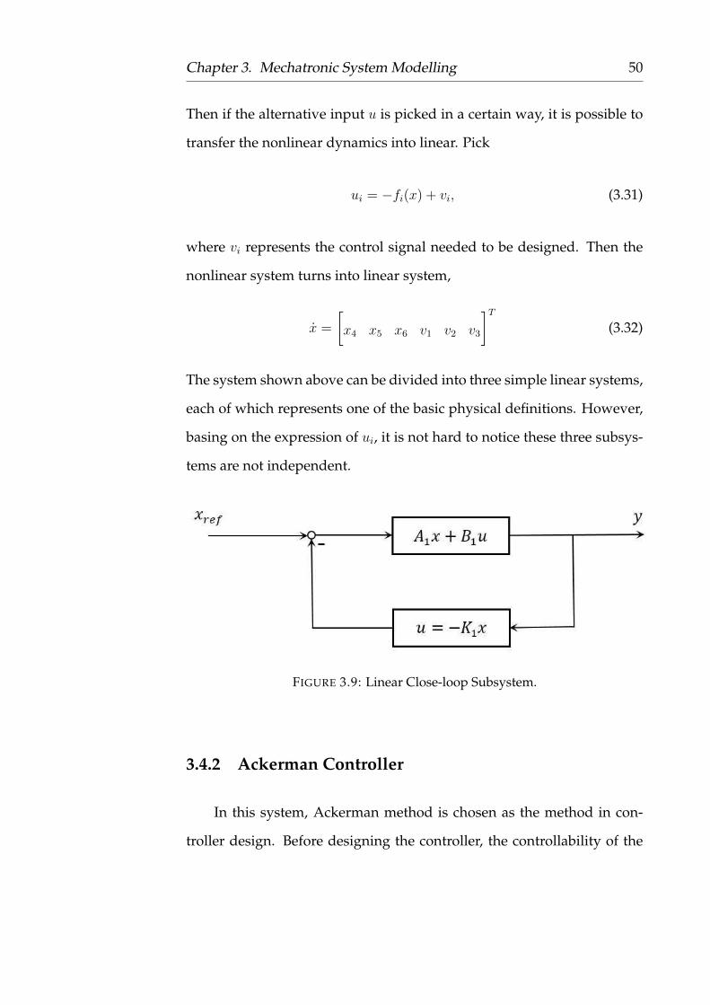
3.9 Linear Close-loop Subsystem. . . . . . . . . . . . . . . . . . 50
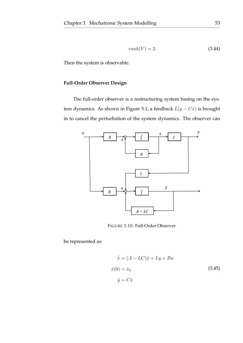
3.10 Full-Order Observer . . . . . . . . . . . . . . . . . . . . . . 53
3.11 Manipulator Simulation. . . . . . . . . . . . . . . . . . . . . 55
4.1 Fault Matrix Observer. . . . . . . . . . . . . . . . . . . . . . 67
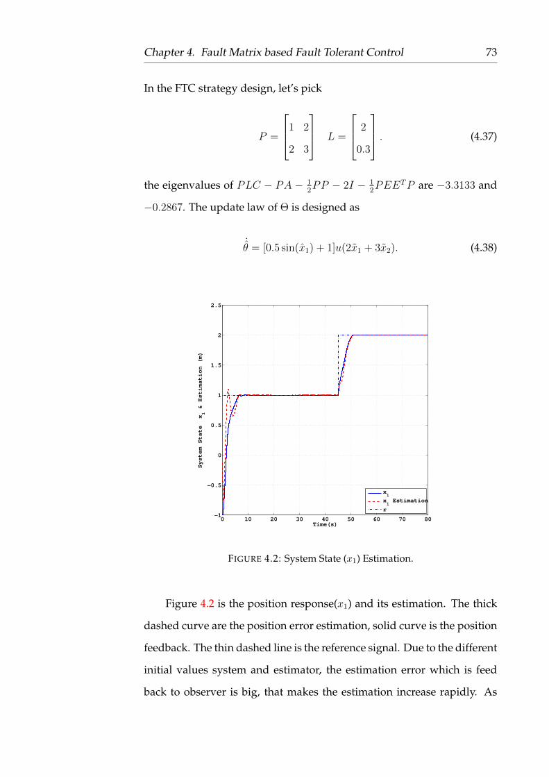
4.2 System State (x1) Estimation. . . . . . . . . . . . . . . . . . 73
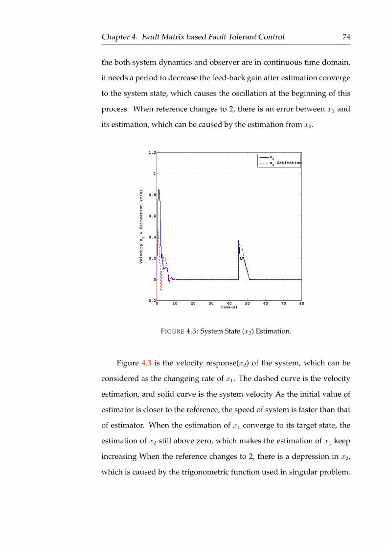
4.3 System State (x2) Estimation. . . . . . . . . . . . . . . . . . 74
Page 6
6
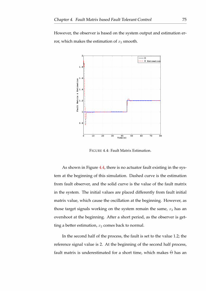
4.4 Fault Matrix Estimation. . . . . . . . . . . . . . . . . . . . . 75
4.5 Disturbance Estimation. . . . . . . . . . . . . . . . . . . . . 76
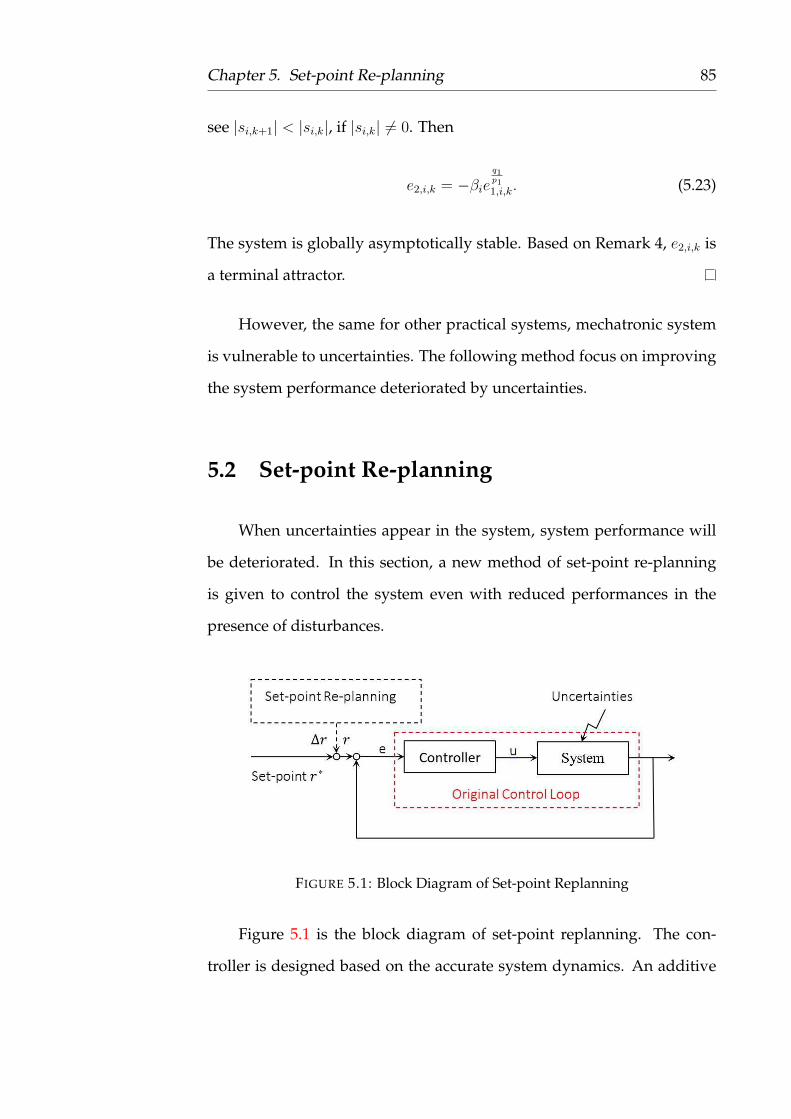
5.1 Block Diagram of Set-point Replanning . . . . . . . . . . . 85
5.2 Holonomic Mobile Robot c©Festo Didactic. . . . . . . . . . 94
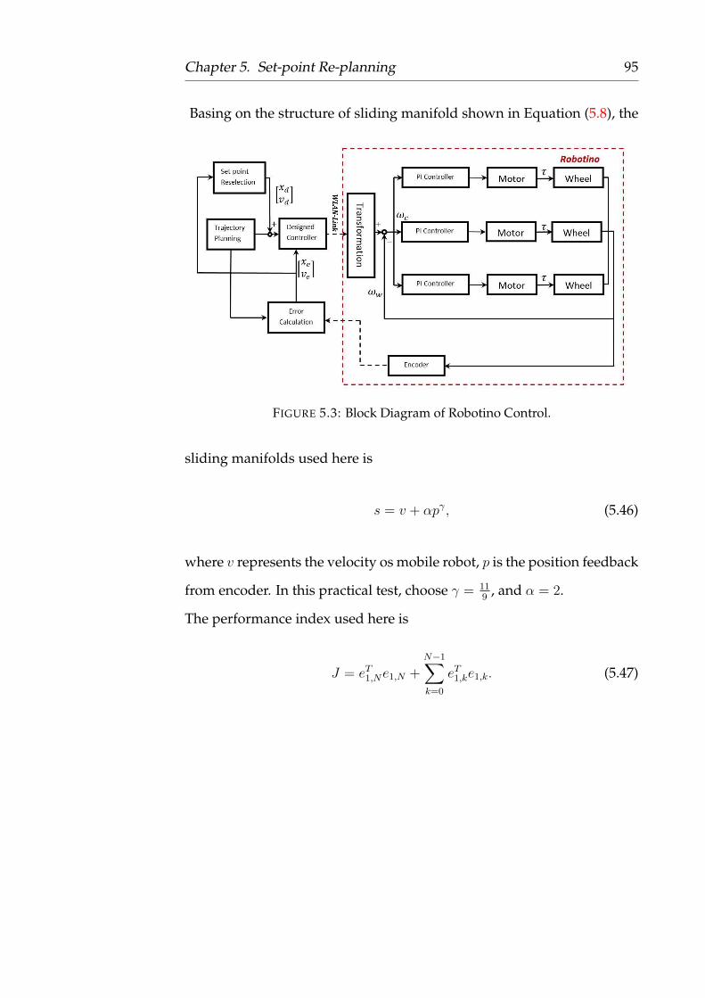
5.3 Block Diagram of Robotino Control. . . . . . . . . . . . . . 95
5.4 Position Error in x Direction . . . . . . . . . . . . . . . . . . 96
5.5 Position Error in y Direction. . . . . . . . . . . . . . . . . . 96
5.6 Velocity in x Direction. . . . . . . . . . . . . . . . . . . . . . 97
5.7 Velocity in y Direction . . . . . . . . . . . . . . . . . . . . . 98
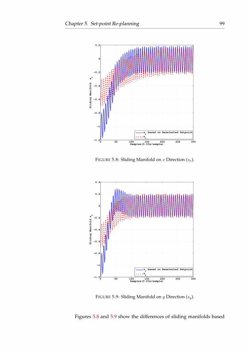
5.8 Sliding Manifold on x Direction (sx). . . . . . . . . . . . . . 99
5.9 Sliding Manifold on y Direction (sy). . . . . . . . . . . . . . 99
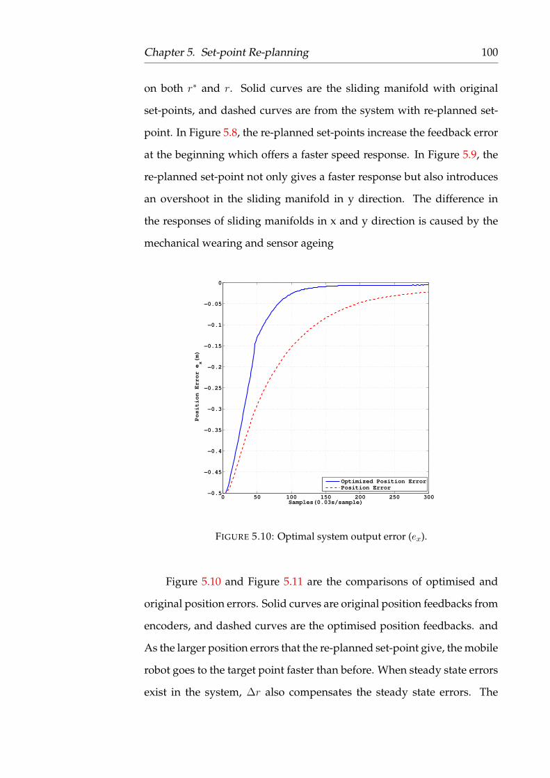
5.10 Optimal system output error (ex). . . . . . . . . . . . . . . . 100
5.11 Optimal system output error (ey). . . . . . . . . . . . . . . . 101
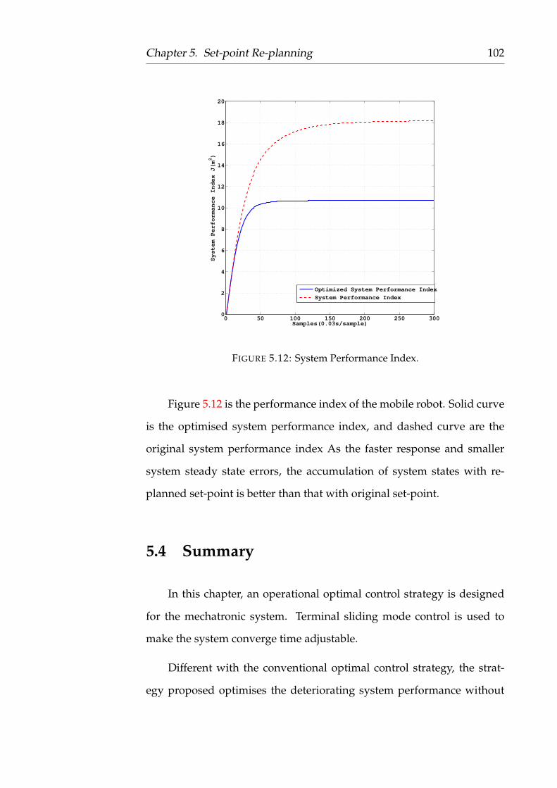
5.12 System Performance Index. . . . . . . . . . . . . . . . . . . 102
Page 7
7
List of Abbreviations
DOF Degree Of Freedom
SMC Sliding Mode Control
TSMC Terminal Sliding Mode Control
DTSMC Discrete Terminal Sliding Mode Control
MIMO Multi-Input Multi-Output
FTC Fault Tolerant Control
DC Direct Current
PI Proportional Integral
HJB Hamilton Jacobi Bellman
LQR Linear Quadratic Regulator
Page 8
8
Abstractby Xiaomo YAN
Control of mechatronic systems remain an open problem in control the-
ory despite the research work worldwide in the last decade. Uncertain-
ties in mechatronic systems, which includes faults, and disturbance, will
often cause undesired behaviours, affecting the systems performances,
may lead to the system failure, or even causing safety issues.
Control reconfiguration is an active approach in control systems field.
However, controller reconfiguration involves changes in its parameters
and structure. System stability might not be able to be guaranteed during
the parameters tuning, which might cause more damage to system stabil-
ity, sometimes may cause safety issues. Due the on-line reconfiguration
has a scope, during which the system stability can not be guaranteed.
This leads that the systems must be turned off during reconfiguration
process. In many industrial areas, such as metallurgy, forging, and man-
ufacturing, shutting down the streamline leads to significant levels of lost
productivity and unacceptable economic losses.
As alternative to control reconfiguration approach, in this thesis two
methods are proposed to deal with faults and disturbances. The first
method is the fault matrix observer and the second one is the set-point
re-planning. The idea of both methods is to compensate the faults and
disturbances which affect the system performances without changing the
controller structure or controller parameters.
Page 9
9
Declaration of Authorship
I, Xiaomo YAN, declare that this thesis titled, “Modelling and Control
of Advanced Mechatronic System” and the work presented in it are my
own. I confirm that:
• This work was done wholly or mainly while in candidature for a
research degree at this University.
• Where any part of this thesis has previously been submitted for a
degree or any other qualification at this University or any other in-
stitution, this has been clearly stated.
• Where I have consulted the published work of others, this is always
clearly attributed.
• Where I have quoted from the work of others, the source is always
given. With the exception of such quotations, this thesis is entirely
my own work.
• I have acknowledged all main sources of help.
• Where the thesis is based on work done by myself jointly with oth-
ers, I have made clear exactly what was done by others and what I
have contributed myself.
Signed:
Date: 13, Jun,2017
Page 10
10
Copyright Statement
• The author of this thesis (including any appendices and/or sched-
ules to this thesis) owns certain copyright or related rights in it (the
’Copyright’) and s/he has given The University of Manchester cer-
tain rights to use such Copyright, including for administrative pur-
poses.
• Copies of this thesis, either in full or in extracts and whether in hard
or electronic copy, may be made only in accordance with the Copy-
right, Designs and Patents Act 1988 (as amended) and regulations
issued under it or, where appropriate, in accordance with licensing
agreements which the University has from time to time. This page
must form part of any such copies made.
• The ownership of certain Copyright, patents, designs, trade marks
and other intellectual property (the ’Intellectual Property’) and any
reproductions of copyright works in the thesis, for example graphs
and tables (’Reproductions’), which may be described in this the-
sis, may not be owned by the author and may be owned by third
parties. Such Intellectual Property and Reproductions cannot and
must not be made available for use without the prior written per-
mission of the owner(s) of the relevant Intellectual Property and/or
Reproductions.
Page 11
11
• Further information on the conditions under which disclosure, pub-
lication 13 and commercialisation of this thesis, the Copyright and
any Intellectual Property and/or Reproductions described in it may
take place is available in the University IP Policy (see http://
documents.manchester.ac.uk/DocuInfo.aspx?DocID=487),
in any relevant Thesis restriction declarations deposited in the Uni-
versity Library, The University Library’s regulations (see http://
www.manchester.ac.uk/library/aboutus/regulations) and
in The University’s policy on presentation of Theses
Page 12
12
AcknowledgementsI would like to express my deepest thanks and sincere gratitude to my su-
pervisor, Prof. Hong Wang , not only for his thoughtful supervision, sin-
cere advice and guidance, but also for his unlimited assistance, valuable
consultation, helpful comments and critical remarks while reviewing the
thesis.
My deep thanks to my supervisor Dr. Alexandru Stancu for his great
support, valuable discussions and helpful comments while reviewing the
thesis.
I would also like to thank Control System Centre at the University
of Manchester for the excellent environment provided for postgraduate
students.
My special and sincere thanks to my beloved family. A special feel-
ing of gratitude to my loving parents, Mingyan Jiang and Wei Yan whose
words of encouragement and push for tenacity ring in my ears.
Last, but not least, I would like to dedicate this thesis to my wife
Ziwei for her love.
Page 13
13
Chapter 1
Introduction
Robotic manipulators are mechatronic systems mimicking the func-
tionality of a human arm. The first robot manipulator was developed in
1947 by Argonne National Laboratory (Goertz 64). Because of its bionic
structure, researches noticed that the robotic manipulator should have a
wider use in industry. The first robotic manipulator patent was filed by
George Devol in 1954, which implies that the value of robotic manipula-
tor has been recognized by industrial sectors.
FIGURE 1.1: Unimate Robot c©Unimation.
Two years later, in 1956, a robotic company called Unimation is founded
by Devol and Joseph F. Engelberger to develop the industrial robot. As
Page 14
Chapter 1. Introduction 14
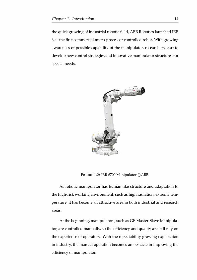
the quick growing of industrial robotic field, ABB Robotics launched IRB
6 as the first commercial micro-processor controlled robot. With growing
awareness of possible capability of the manipulator, researchers start to
develop new control strategies and innovative manipulator structures for
special needs.
FIGURE 1.2: IRB-6700 Manipulator c©ABB.
As robotic manipulator has human like structure and adaptation to
the high-risk working environment, such as high radiation, extreme tem-
perature, it has become an attractive area in both industrial and research
areas.
At the beginning, manipulators, such as GE Master-Slave Manipula-
tor, are controlled manually, so the efficiency and quality are still rely on
the experience of operators. With the repeatability growing expectation
in industry, the manual operation becomes an obstacle in improving the
efficiency of manipulator.
Page 15
Chapter 1. Introduction 15
Manipulator control is an important research in nonlinear system
control. In the trajectory control, the speed control is used to guarantee
that the end-effector will track set trajectory. As the dynamics of manipu-
lator has strong non-linearities, and system states are highly coupled, the
controller must have a good dynamic response and be adapt at stabiliz-
ing the nonlinear terms.
Proportional–integral–derivative (PID) controller is one of the famous
control strategies used in manipulators control due to its easy tuning
structure [1–3]. However, the easy parameter tuning brings some disad-
vantages. Because the tuning of PID is based on the system output, which
means the inner relationships of system states are ignored during the tun-
ing The neglect of the inner relationships of system states always cause
a energy waste. For instance, when the speed of system responses is in-
creased by the proportional coefficient, overshoots are introduced at the
same time. Then derivative coefficient has to be increased to reduce the
overshoot, which means derivative term goes against the proportional
term in the same PID controller.
Another control method widely used in industry is variable struc-
ture control (VSC). VSC is a discontinuous control method, achieving the
stability by switching between different controller structures. There are
two types of VSC, bang-bang control and sliding mode control. The con-
trol law used in bang-bang control is relay, which stabilizes the system by
thresholds of tracking errors. However, bang-bang control can only sta-
bilize the system states in the range of thresholds. Different with bang-
bang control, the states related structures used in sliding mode control
(SMC) can make the tracking a time variant reference. By choosing dif-
ferent structures of nonlinear sliding manifolds, the SMC is adaptable to
rapidly-change system states. As the sliding mode control is based on
Page 16
Chapter 1. Introduction 16
the system dynamics, it is easier to analysis system stability of SMC than
that of PID.
FIGURE 1.3: Closed-loop System with Chattering in theoutput.
Figure 1.3 is the block diagram of the closed-loop system. Sliding
mode controller (SMC) is used as the control strategy. The convergence
speed is always described qualitative, such as ’fast converge’ and ’slow
converge’. In this thesis an analytical solution of converge time is pro-
posed, such that the convergence speed can be described more precisely.
Because of the imperfections in real systems in reality SMC always presents
the chartering phenomenon.
FIGURE 1.4: Closed-loop System affected by Uncertainties.
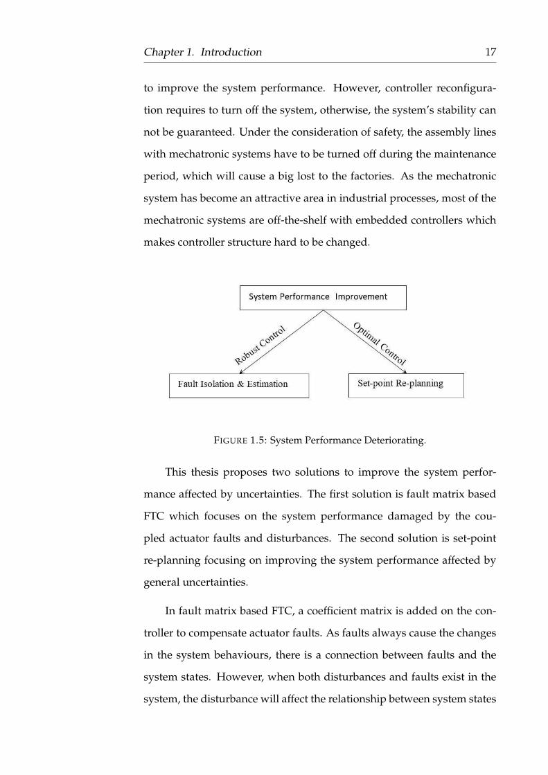
Uncertainties, which includes faults and disturbance, always deteri-
orate the system performance. Controller reconfiguration is always used
Page 17
Chapter 1. Introduction 17
to improve the system performance. However, controller reconfigura-
tion requires to turn off the system, otherwise, the system’s stability can
not be guaranteed. Under the consideration of safety, the assembly lines
with mechatronic systems have to be turned off during the maintenance
period, which will cause a big lost to the factories. As the mechatronic
system has become an attractive area in industrial processes, most of the
mechatronic systems are off-the-shelf with embedded controllers which
makes controller structure hard to be changed.
FIGURE 1.5: System Performance Deteriorating.
This thesis proposes two solutions to improve the system perfor-
mance affected by uncertainties. The first solution is fault matrix based
FTC which focuses on the system performance damaged by the cou-
pled actuator faults and disturbances. The second solution is set-point
re-planning focusing on improving the system performance affected by
general uncertainties.
In fault matrix based FTC, a coefficient matrix is added on the con-
troller to compensate actuator faults. As faults always cause the changes
in the system behaviours, there is a connection between faults and the
system states. However, when both disturbances and faults exist in the
system, the disturbance will affect the relationship between system states
Page 18
Chapter 1. Introduction 18
and actuator faults. If actuator fault can be isolated from disturbance, ac-
tuator faults can be compensated without changing controller structure.
In most instances, different kinds of uncertainties exist in the system
and are coupled to each other. To optimise system performance, opti-
mal control methods are always applied on the system. However, the
conventional system optimisation is also based on controller reconfigu-
ration. It will be convenient if we can find a method that optimises the
system performance, which is damaged by uncertainties, without chang-
ing controller.
1.1 Research Questions
• How can be computed analytically the convergence time for the
reaching phase in case of SMC?
• How to isolate, estimate and eliminate the actuator faults in the
nonlinear system when it is coupled with disturbance without chang-
ing controller?
• How to control the systems, even with reduced performances, in
presence of faults or any other types of disturbances without mod-
ifying the controller structure or parameters?
1.2 Thesis Objectives
This section gives a summary of the thesis objectives which are listed
as follows:
Page 19
Chapter 1. Introduction 19
• Investigating the effectiveness of nonlinear control design for con-
tinuous nonlinear system, as well as for discrete nonlinear system
using a special nonlinear structure.
• Designing a new fault tolerant control strategy for continuous time
kinematic systems subject to faults and disturbances, using fault
matrix to link actuator fault to control signal.
• Introducing a novel discrete time system optimisation strategy to
mechatronic systems subject to uncertainties without changing the
original closed-loop.
Page 20
Chapter 1. Introduction 20
1.3 Structure of Thesis
The rest of the thesis is organised as follows:
Chapter 2 contains a state of the art in areas related to this thesis.
In addition, some important stability theorems are introduced to help to
understand the methods proposed in this thesis.
Chapter 3 presents the modelling of n-DOF manipulator based on
Newton-Euler method. Then, parameters from ABB IRB 120 are used in
the Matlab based 3-DOF manipulator visualization program design. To
make the visualization program practical, both full-order observer and
reduced-order observer are implemented.
Chapter 4 introduces a fault matrix based FTC strategy. A terminal
slide mode control strategy is chosen to guarantee the system stability. In
addition, a fault matrix observer is designed to observe the relationships
between control signals and actuator faults.
Chapter 5 presents a novel operational control method. HJB equa-
tion is used to optimise the system performance. Due to the Cascade
control structure used in the design, multi-rate method is implemented
to reduce the affect from the delay between the outer loop and the inner-
loop.
Chapter 6 presents the conclusion and suggestions for future work.
Page 21
21
Chapter 2
Control Background and
Preliminaries
2.1 Control Background
2.1.1 Mechatronic Systems
There are two types of techniques in finding manipulator dynamics,
numerical and symbolical. However, before any of the techniques can be
used, the problem of complexity need to be solved [4–14]. In 1972, Paul
[15] presented a numerical solution of finding configuration-dependent
6-DOF manipulator based on force balance. Targets are recognized by the
information given by vision subsystem, and then the strategy subsystem
guarantees that the arm is capable of grabbing the target cube. In 1977,
a general symbolical 3-DOF dynamics is given by using Euler-Lagrange
formula [16]. It is clear to see that the torques of the motors are related
to angles, angular velocities and other constant parameters of the manip-
ulator. They also considered the offset of links to make their dynamics
more adaptable. But it is also clear to see that the symbolic technique is
only available in small DOF structure for the reason of complexity.
Page 22
Chapter 2. Control Background and Preliminaries 22
Indeed, it may not necessary to have all the details of manipulator
in control strategy design. But it turns out that Coriolis and centripetal
can be ignored to simplify the dynamics not only in low speed but also
high speed situations [17]. The dynamics left is still not ’brief’ enough to
be used in design, and people have never stop finding a more efficient
expression. As we can see that the most complex part in manipulator
dynamics is brought in by the inertia tensor, the dynamics will be sim-
plified greatly if they can be decoupled. Youcef-Touml and Asada [18]
attempted to solve this decoupling question in 1985. It turns out that
those components can only be decoupled when the revolute joints have a
specific structure, which is all joint axes must be orthogonal to each other.
In 1984, Tarn et al. [19] figure out a method called "External Linearisa-
tion, which remains more system features than Jacobian method. More-
over, a necessary and sufficient condition of decoupling is also given in
this paper. Kosuge and Furuta used Jacobian matrix to deduce the linear
mode. However, the disadvantage of Jacobian matrix is that the system
dynamics is linearised around a nominal point, which makes their dy-
namics only suitable for those slow-change processes [20]. Later in 1991,
Yurkovich et al. [21] applied feedback linearisation onto the manipulator
dynamics. By using this method, all the nonlinear components are elim-
inated by the first part of the controller, then the rest part of controller
only need to focus on maintaining the stability of a second order system
that represents the fundamental physical relationship.
Additionally, for a better understanding of the behaviours of manip-
ulator, a clear physical insight of manipulator is crucial [22, 23]. As a
result of the complex dynamics, the computation related manipulators
is always slow. It is essential to find a more efficient way to deal with
manipulator dynamics in the computer program. In 1981, Hewit and
Page 23
Chapter 2. Control Background and Preliminaries 23
Burdess [24] brought a fast control method by observing torque.
2.1.2 Sliding Mode Control
Sliding mode control (SMC) is known for its outstanding robust-
ness[25–34]. The SMC design can be considered as a mathematical ex-
planation of one basic reaction from actual operators. The sliding mode
controller is discontinuous, which can jump from one continuous surface
to another one. Utkin [35] proposed an idea of variable structure system
(VSS) control design. Furthermore, he also proved the existence of sliding
mode surface. Basing on Utkin’s method, Young [36] presented a prac-
tical example of SMC on 2-DOF manipulator. To apply the SMC control
strategy into practical processes, discrete time SMC control stability has
been proved based on a pair of selected state feedback control signal [37].
The amplitude of control has to be as small as possible, which is contrary
to the continuous system [38].
In 1996, Mnif et al. applied holonomic constraints to the manipulator
dynamics in SMC design. However, as problems were shown in these
methods [39–41], chattering phenomenon has long been a notable issue
in the SMC design. Those high-frequency components, which caused by
the ideal switch, will not only affect the system response but also damage
the switches of plants. To eliminate the chattering phenomenon, smooth
functions, such as saturation function, are usually used in the SMC de-
sign [42]. When the sliding manifold moves within the scope of the cho-
sen linear portion, the amplifier from saturation function slows the re-
sponse. As a good controller strategy, the convergence of the controller
need to be enhanced. Terminal sliding mode control (TSMC) had been
Page 24
Chapter 2. Control Background and Preliminaries 24
introduced in the early 90s, which guarantees the finite convergence time
[43–45].
In 1997, a new terminal sliding manifold had been proposed by Man
and Yu to guarantee the finite convergence for a type of linear MIMO
kinematic system [46]. The convergence time has been proved in the pa-
per, but the part that pulls the system states back to manifold remains
to be discontinuous. Young et al. [47] presented a practical SMC guide,
in which, boundary layer control was mentioned. Boundary layer con-
trol focuses on reducing the effect of chattering by replacing switching
function with the designed parasitic dynamics. But the boundary layer
control is doing a trade-off between chattering reduction and disturbance
rejection, which means it is necessary to find a balance between steady
state error and chattering. As the nonlinear sliding manifold introduced,
a singular problem has to be considered.
In 2002, a non-singular TSMC manifold has been proposed with an
additional limitation on the manifold parameter selection [48]. In the
conventional SMC design, a fast response relies on a large control gain,
which is another incentive of the chattering issue. Instead of using a lin-
ear function, nonlinear sliding manifolds give a more ’flexible’ response
[49–53]. To solve the chattering problem, Levant [54] proposed a high-
order SMC method, which is capable of guaranteeing the finite-time con-
vergence. The high-order SMC can reduce chattering while remaining
the robustness. The boundary of uncertainties and system relative de-
gree are needed. TSMC can only guarantee the system states converge to
the set-point within finite time, Polyakov [55] pointed out a certain type
of function, which guarantees a fast reach time with both large and small
variances. The consideration of their function is based on both fast con-
vergences on the small scalar and others. To approach the requirement,
Page 25
Chapter 2. Control Background and Preliminaries 25
they use the differences between different system states powers. Then on
account of the similar idea, the pull-back part is based on the norm of the
manifold.
2.1.3 Fault Tolerant Control
As the control theory has been approved by industry, the quality of
industrial products relies on control strategies more than ever [56–65].
Sometimes robustness is used to guarantee that controllers are capable of
working under harsh situations. However, there are demands for high
system performance, the robustness is always limited, which means the
inherent controller may not be able to guarantee the performance any
more when extra faults occur. Faults occur for many reasons, such as
ageing, temperature changing, and humidity increasing. Aiming for bet-
ter reliability and safety, the importance of fault tolerant control has been
increasingly recognized by more and more people [66–70]. By using the
fault tolerant control strategy, the system can continue working with a
reduced level performance rather than fail completely.
Fault tolerant control becomes challenging not only because of the
increasing the complexity of systems, but also the states coupling with
disturbance. Increasing the efficiency of the control strategy, accurate sys-
tem states value are needed. But in many practical industrial cases, states
required are not only the system outputs but also those hidden inside the
equipment. To achieve all the parameters needed, it is necessary to find
a way to gather those internal states. The observer is now a common
method used in control strategy design. The observer is mostly designed
by the computation based on knowledge of original system structure [71–
Page 26
Chapter 2. Control Background and Preliminaries 26
80]. By finding the mathematical relationships between observable sys-
tem outputs and states, those internal states’ value can be calculated.
There are two basic linear system state observer methods, full-order
and reduced order state observers [81]. The full-order observer is based
on the system output values and knowledge of system model. But some-
times, the system outputs are parts of the system states. It means there
might be another way to design the observer only for the states not in-
cluded in the output, which is named reduced-order observer. As most
of the practical industrial processes are nonlinear systems; it is neces-
sary to find methods that can estimate system states from nonlinear sys-
tems. The main idea of nonlinear observer designs [82], such as extended
Kalman filter, linearise the system around equilibrium points, then by us-
ing the constraints of systems, such as Lipschitz condition, to find out the
boundary of the Lyapunov candidate.
The internal relationships among sensor fault, actuator fault and dis-
turbance cannot be ignored during the strategy design. If those uncer-
tainties can be decoupled, it is possible to design an observer to estimate
the fault. To eliminate the disturbance, either disturbance observer or in-
crease the robustness of the controller can be used. For instance, Capisani
et al. [83] proposed two sliding mode control based fault observer when
either sensor fault or actuator fault occurs in the system. The basic idea
of fault matrix is representing the actuator faults basing on its relation-
ship with control inputs. Different from disturbance, faults always relate
to the system states [84]. Instead of analysing the linear system stability,
boundary of Jacobian matrix can also be used in tracking error analysis
to make sure zero is an equilibrium point of the observer [85].
However, the observer based strategy is not the only way to design
Page 27
Chapter 2. Control Background and Preliminaries 27
fault tolerant control strategy. Marx et al. [86] applied a H∞ filter to Youla
parametrized controller to minimize the responses of exogenous inputs.
In 2015, an adaptive fault tolerant control strategy was proposed by Liu
and his co-workers [87], the system they focus on is Markovian jump
system with constant parameters in each period. Both actuator fault and
disturbance have been considered.
In 2016, Defoort et al. [88] proposed an adaptive super-twisting ac-
tuator fault observer. However, super-twisting only works for second-
order system, which makes his method difficult to extend to higher order
system. The observer designed focus on estimate the real value of system
states, which means the state observer proposed only guarantee distur-
bance will not make system unstable. Actuator fault is approximated by
integrating the sign of estimation error, which reduce the chattering. But
due to the constant coefficient used in the fault estimation, the proposed
fault observer can only compensate the actuator fault roughly.
In 2017, Zhang et al. [89] proposed an adaptive fault-tolerant con-
trol strategy. Actuator fault is expressed by using control signal and bias
signals. The un-modelled nonlinear part in system is described by fuzzy
hyperbolic model, which transfer the non-linear system in to linear func-
tional. A fuzzy system state observer is designed based on the system
linear functional. However, disturbance is compensated by its boundary,
which means the proposed method can only improve the damage comes
from actuator fault, and guarantee the disturbance will not make the sys-
tem unstable.
Li et al. [90] proposed an adaptive fault tolerant control strategy in
2017. The proposed method focus on the SISO nonlinear system. A fuzzy
Page 28
Chapter 2. Control Background and Preliminaries 28
system states observer is designed. The un-modelled nonlinear part is ex-
pressed by fuzzy logic model. The actuator fault is expressed by control
signal. However, in their design, disturbance has not been taken into con-
sideration, which means their method cannot isolate actuator fault from
disturbance.
2.1.4 System Optimisation
The motive of optimal control theory is trying to find a result from
any possible solutions based on dynamic programming and maximum
principle [91–100]. To achieve the optimal value, feedback regulation is
always used in the design [101]. In 1961, Desoer et al. [102] presented a
force optimal tracking strategy, which not only guarantees the minimum
sample periods but also proves its finite time convergence. In the same
year, Smith [103] found a time-optimal method for high-order system,
which has a constraint of constant control signal value. His method is
based on optimising the switch time, but with the constant control signal
he used, chattering cannot be ignored. Instead of optimising the switch
time, a HJB based obstacle avoidance algorithm is proposed following
pseudo return function in 1997 [104]. In 2000, LQR method had been
applied on self-turning relay system [105]. To guarantee the fast conver-
gence, an auxiliary output had also been designed. However, conven-
tional optimal controls have focused on improving system performance
by optimising controller parameters, which is hard to . In 2014, T. Chai, S.
Qin, and H. Wang [106] proposed the idea of optimal operational control
for complex industrial processes. However, only the possible research
directions are given, methods to realize the ideas still remain to be open
Page 29
Chapter 2. Control Background and Preliminaries 29
questions. The main idea of the optimal operational control is to opti-
mise the damaged system performance on-line [107–110]. For the shake
of safety, the original control closed-loop is considered as inaccessible.
A. Wang, P. Zhou and H. Wang [111] proposed a set-point reselection
method for stochastic system. The reselected set-point is used to reshape
the system performance curve. The trough of performance curve has
been widen, so that the system performance is easier to converge the op-
timal point. However, only a brief mathematical description has been
given to generalize the idea. The authors also indicated that the conver-
gence of the set-point reselection remains to be an open question.
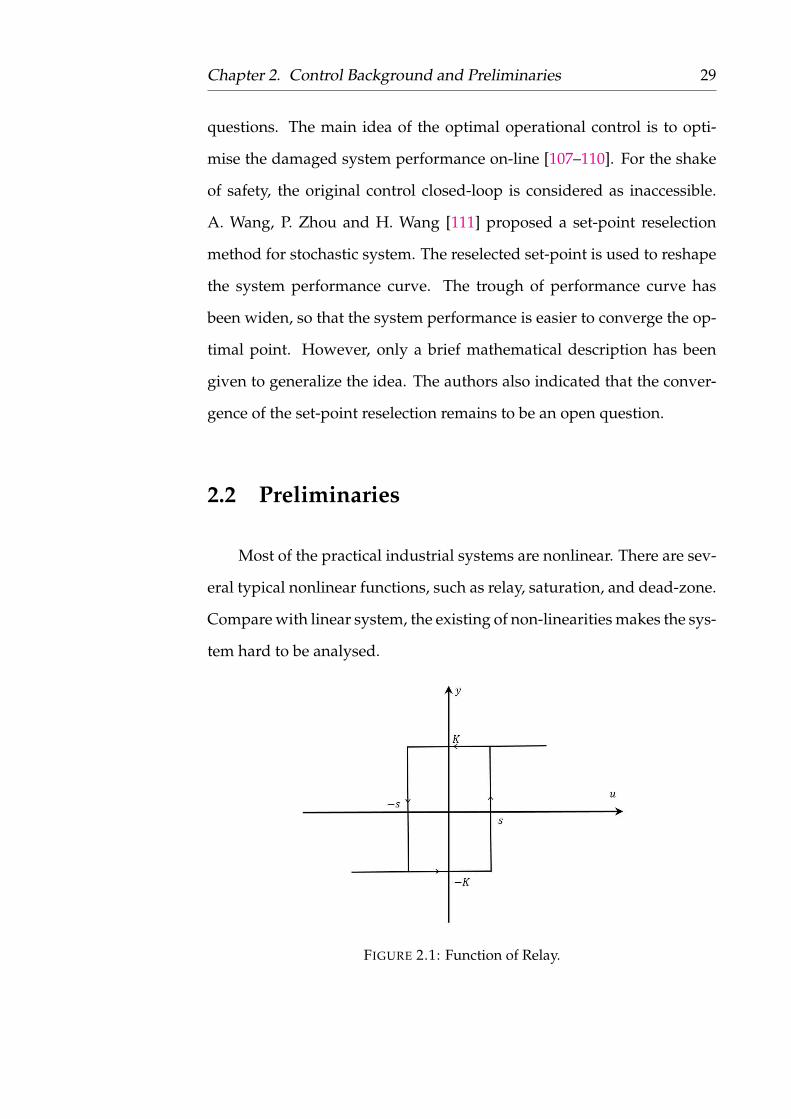
2.2 Preliminaries
Most of the practical industrial systems are nonlinear. There are sev-
eral typical nonlinear functions, such as relay, saturation, and dead-zone.
Compare with linear system, the existing of non-linearities makes the sys-
tem hard to be analysed.
FIGURE 2.1: Function of Relay.
Page 30
Chapter 2. Control Background and Preliminaries 30
FIGURE 2.2: Function of Saturation.
FIGURE 2.3: Fuction of Dead-zone.
Page 31
Chapter 2. Control Background and Preliminaries 31
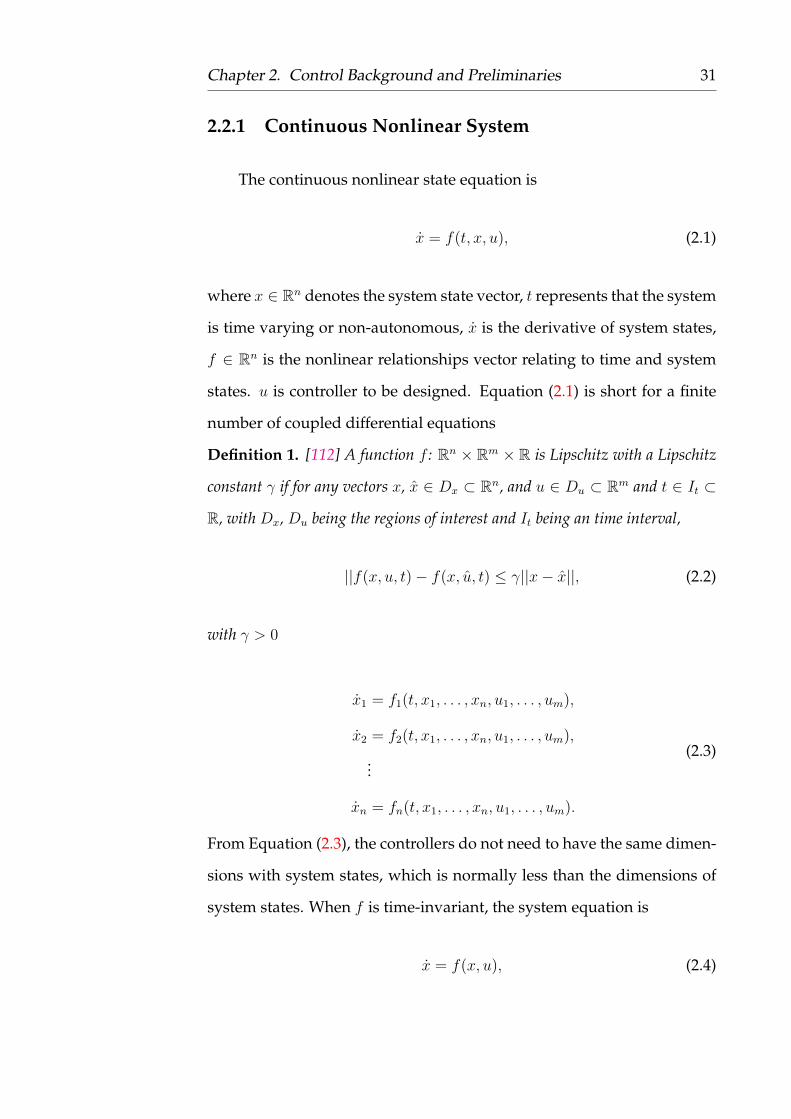
2.2.1 Continuous Nonlinear System
The continuous nonlinear state equation is
x = f(t, x, u), (2.1)
where x ∈ Rn denotes the system state vector, t represents that the system
is time varying or non-autonomous, x is the derivative of system states,
f ∈ Rn is the nonlinear relationships vector relating to time and system
states. u is controller to be designed. Equation (2.1) is short for a finite
number of coupled differential equations
Definition 1. [112] A function f : Rn × Rm × R is Lipschitz with a Lipschitz
constant γ if for any vectors x, x ∈ Dx ⊂ Rn, and u ∈ Du ⊂ Rm and t ∈ It ⊂
R, with Dx, Du being the regions of interest and It being an time interval,
||f(x, u, t)− f(x, u, t) ≤ γ||x− x||, (2.2)
with γ > 0
x1 = f1(t, x1, . . . , xn, u1, . . . , um),
x2 = f2(t, x1, . . . , xn, u1, . . . , um),
...
xn = fn(t, x1, . . . , xn, u1, . . . , um).
(2.3)
From Equation (2.3), the controllers do not need to have the same dimen-
sions with system states, which is normally less than the dimensions of
system states. When f is time-invariant, the system equation is
x = f(x, u), (2.4)
Page 32
Chapter 2. Control Background and Preliminaries 32
Equation (2.4) is an overview of the nonlinear system, which includes all
components in f . However, it is necessary to find an expression which
can demonstrate more details of the system.
x = Ax+ f(x) + g(x)u, (2.5)
where Ax represents the linear part related to system states, f(x) denotes
the system inner structure, g(x) is the relationship between the controller
and system inputs.
2.2.2 Discrete Time Nonlinear System
As shown in Figure 2.4, the discrete time nonlinear system can be
considered as a sampled continuous nonlinear system with sampling
time T . The discrete time nonlinear state equation is
xk+1 = f(xk, uk), (2.6)
where xk represents the kth sample of system state, f is nonlinear rela-
tionships relating to system states xk and control input uk.
2.3 Stability Theory
2.3.1 Continuous Time Systems
A key area of control engineering is stability theory. Controllers are
designed to guarantee the stability of system. One of the foundations of
Page 33
Chapter 2. Control Background and Preliminaries 33
FIGURE 2.4: Discrete Nonlinear System.
the equilibrium point is Lyapunov function. System described in Equa-
tion (2.4) with a state feedback controller can be rewritten as
x = f(x), (2.7)
Definition 2. The equilibrium point x = 0 in Equation (2.7) is
• stable if, for each ε > 0, there is δ = δ(ε) > 0 such that
||x(0)|| < δ ⇒ ||x(t)|| < ε,∀t ≥ 0. (2.8)
• unstable if it is not stable.
• asymptotically stable if it is stable and δ can be chosen such that
||x(0)|| < δ ⇒ limt→∞
x(t) = 0. (2.9)
Theorem 2.3.1 (Lyapunov Stability Theorem). Let x = 0 be an equilibrium
point for (2.7) and D ⊂ Rn be a domain containing x = 0. Let V :D → R be a
Page 34
Chapter 2. Control Background and Preliminaries 34
continuously differentiable function such that
V (0) = 0 and V (x) > 0 in D − {0}
V ≤ 0 in D.
Then, x = 0 is stable. Moreover, if
V (x) < 0 in D − {0}.
then x = 0 is asymptotically stable.
Theorem 2.3.2 (LaSalle’s Invariance Principle Theorem). For autonomous
systems, let D ⊂ Rn be a domain containing the equilibrium point of origin. If
there exists a continuously differentiable, positive definite function V : D → R
such that
V =∂V
∂x= −W (x) ≤ 0 (2.10)
in D. Let
S = {x ∈ D|V (x) = 0}, (2.11)
and suppose that no solution can stay identically in S, other than the origin.
Then, the origin is asymptotically stable.
In addition, if D = Rn and V is radially unbounded, the origin is globally
asymptotically stable.
Remark 1. The candidate chosen in this thesis is the square of system state,
which enables the candidate to be an expression of energy consumption.
Remark 2. Because the Lyapunov candidate is also the sum of the square of
system states, it is obvious that the candidate will greater than 0 when x 6= 0.
To make sure the system is stable, the L2 distance of system states need to be
bounded, which means the feasible domain of the system states will be a round
area. So the derivation of the candidate is less than or equal to 0. If the derivative
of the candidate is less than 0, the Lyapunov candidate is describing a system
whose states are stable in a smaller round than the one picked initially. As the
Page 35
Chapter 2. Control Background and Preliminaries 35
feasible domain goes smaller and smaller, system states will go to the original
point of the area x = 0, which is asymptotically stable.
2.3.2 Discrete Time Systems
Nonlinear time varying discrete system can be written as
xk+1 = f(xk), (2.12)
where x ∈ Rn, and f ∈ Rn.
Definition 3. Consider the system (2.12), V changes to ∆V of the form
∆Vk+1 = V (xk+1)− V (xk). (2.13)
Corollary 1 ([37]). The equilibrium point 0 is locally stable in the sense of
Lyapunov if there exists a positive definite Lyapunov candidate V (xk) such that
∆Vk+1 ≤ 0, (2.14)
for k ≥ k0 and all x such that ||x|| < r for some r > 0 in a deleted neighbourhood
of 0.
2.4 Summary
In this chapter, a state-of-the-art on the recent methods in mecha-
tronic systems, sliding mode control, fault tolerant control, and system
optimisation is provides. There are highlighted the last achievements in
each domain together with the open research topics which are addressed
in this thesis. Because one of the most important problems in control
Page 36
Chapter 2. Control Background and Preliminaries 36
community is the stability analysis, some fundamental definitions and
theorems are provided at the end of this chapter. These concepts will be
used in the rest of the thesis for prove the proposed theorems.
Page 37
37
Chapter 3
Mechatronic System Modelling
As mechatronic system modelling involves mechanical engineering,
electrical engineering, and materials engineering, the dynamics of the
mechatronic system is extremely complex. It is necessary to understand
the principles used in the mechatronic system before the design of con-
troller.
Robotic manipulators are widely used in industrial processes nowa-
days. The rigid n-DOF is driven by n motors, which are located at the
joints. Motors generate the necessary torques in movements. There are
two conventional methods of deriving the dynamics of robotic manipu-
lator, Newton-Euler formulation and Lagrangian formulation. These two
approaches are based on the two different but coexistent balances in all
systems.
Newton-Euler formulation builds on the force balance. Instead of
considering a complex mechatronic system, the process can be simplified
by moving the end point into the target area. With this simplification,
an involute process turns into a combination of rotations and transport-
ing, which perfectly fits into Newton-Euler method. Additionally, as the
kinematic system is practical, energy balance should also be satisfied dur-
ing the processes, which means Lagrangian method can also be used to
Page 38
Chapter 3. Mechatronic System Modelling 38
achieve the dynamics. Because of the consistent result between Newton-
Euler method and Lagrangian method, the Newton-Euler method is used
in the thesis.
3.1 Frame and Rotation
Before starting achieving the dynamics of manipulator, it is neces-
sary to considering two questions, how to describe the similar functions
of each joint and how to map those functions into the same frame. In this
part, definitions of frames and rotation matrices are given.
3.1.1 Frame
There are four basic frames used in the derivative of kinematic sys-
tem.
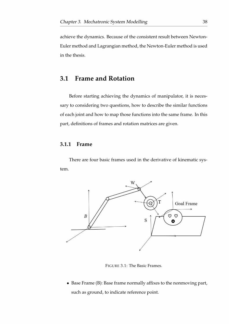
FIGURE 3.1: The Basic Frames.
• Base Frame (B): Base frame normally affixes to the nonmoving part,
such as ground, to indicate reference point.
Page 39
Chapter 3. Mechatronic System Modelling 39
• Station Frame (S): Station frame is a task relevant frame, which in-
dicates the working area of the kinematic system.
• Wrist Frame (W): Wrist frame represents the coordinate on the last
joint of kinematic system.
• Tool Frame (T): Tool frame affixes to the end effector.
Figure 3.2 represents point P in a frame. The position of P can be ex-
pressed as
FIGURE 3.2: Point P in Frame A.
AP =
Px
Py
Pz
, (3.1)
where Px, Py and Px represent the positions of P along axes XA, YA and
ZA respectively.
3.1.2 Rotation
As shown in Figure 3.1 and Figure 3.2, the description of a point
not only relate to its position but also relate to the frame category. For
example, targets are always described by the position relates to station
Page 40
Chapter 3. Mechatronic System Modelling 40
frame SP ; meanwhile, end effector is described by the position relates
to tool frame TP . It is necessary to find a way to transfer positions that
relate to different frames into one frame.
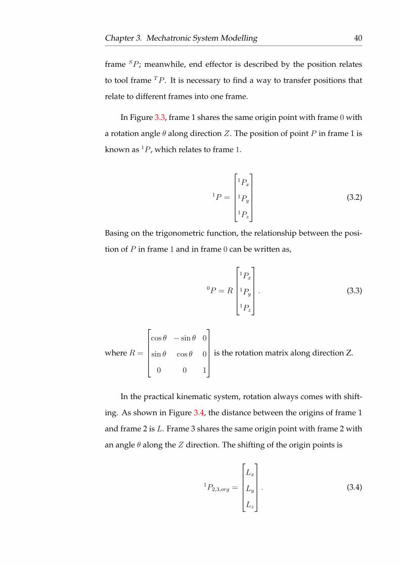
In Figure 3.3, frame 1 shares the same origin point with frame 0 with
a rotation angle θ along direction Z. The position of point P in frame 1 is
known as 1P , which relates to frame 1.
1P =
1Px
1Py
1Pz
(3.2)
Basing on the trigonometric function, the relationship between the posi-
tion of P in frame 1 and in frame 0 can be written as,
0P = R
1Px
1Py
1Pz
. (3.3)
where R =
cos θ − sin θ 0
sin θ cos θ 0
0 0 1
is the rotation matrix along direction Z.
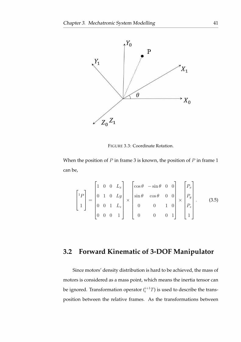
In the practical kinematic system, rotation always comes with shift-
ing. As shown in Figure 3.4, the distance between the origins of frame 1
and frame 2 is L. Frame 3 shares the same origin point with frame 2 with
an angle θ along the Z direction. The shifting of the origin points is
1P2,3,org =
Lx
Ly
Lz
. (3.4)
Page 41
Chapter 3. Mechatronic System Modelling 41
FIGURE 3.3: Coordinate Rotation.
When the position of P in frame 3 is known, the position of P in frame 1
can be,
1P
1
=
1 0 0 Lx
0 1 0 Ly
0 0 1 Lz
0 0 0 1
×
cos θ − sin θ 0 0
sin θ cos θ 0 0
0 0 1 0
0 0 0 1
×
Px
Py
Pz
1
. (3.5)
3.2 Forward Kinematic of 3-DOF Manipulator
Since motors’ density distribution is hard to be achieved, the mass of
motors is considered as a mass point, which means the inertia tensor can
be ignored. Transformation operator (i+1i T ) is used to describe the trans-
position between the relative frames. As the transformations between
Page 42
Chapter 3. Mechatronic System Modelling 42
FIGURE 3.4: Frames Transfer.
frames are invertible, we have i+1i T =i
i+1 T−1. The position matrix (iP ) of
a point in the ith frame can be transferred into the (i+ 1)th frame as,
i+1P =i+1i T iP. (3.6)
The method used here to derivate the manipulator dynamics is Newton-
Euler’s dynamics formulation [113]. Based on Newton’s second law, the
change of movement is related to its acceleration. As the constant length
every link has, changes of accelerations are only related to the angular
velocities.
The force of each joint has two components, the force needed to track
the trajectory and the force used to eliminate effects from other links. In
this part, the expression of the angular velocity of the (i+1)th link, which
is effected by the ith link, is given. The angular velocity of the (i + 1)th
link is
i+1ωi+1 =i+1i Riωi + θi+1
i+1Zi+1, (3.7)
Page 43
Chapter 3. Mechatronic System Modelling 43
where i+1ωi+1 is the angular velocity of (i+ 1)th link. i+1i R is the rotation
matrix from the ith link to the (i+ 1)th link. iωi is the angular velocity of
the ith link related to the ith frame. θi+1 is the increment of the (i+1)th an-
gle. i+1Zi+1 =
0
0
1
is the axis that the (i+ 1)th joint rotates along. i+1i Riωi
represents the shift caused by the rotation of the ith link. θi+1i+1Zi+1 is
the angular velocity needed for the (i + 1)th link. Then it is easy to have
the angular acceleration of the (i+ 1)th joint.
i+1ωi+1 =i+1i R iωi +i+1
i R iωi × θi+1i+1Zi+1 + θi+1
i+1Zi+1, (3.8)
where θi+1 is the angular acceleration needed to change θi+1. The pur-
pose of the outer interactions is to have the (i + 1)th link dynamics, use
θi+1i+1Zi+1 to represent the change of the frame.
i+1vi+1 = i+1i R[iωi × iPi+1 + iωi × (iωi × iPi+1) + ivi], (3.9)
where iPi+1 is the target position from the (i + 1)th frame into the ith
frame.
i+1vCi+1=i+1ωi+1 × i+1PCi+1
+ i+1ωi+1 × (i+1ωi+1 × i+1PCi+1)
+ i+1vi+1.
(3.10)
According to Newton’s Law, the force needed for reaching the designed
speed is
i+1Fi+1 = mi+1i+1vCi+1
. (3.11)
Page 44
Chapter 3. Mechatronic System Modelling 44
The force exerted on the ith joint from its neighbour is
ifi = ii+1R
i+1fi+1 + iFi. (3.12)
When talk about the rotation of rigid body, inertia tensor needs to be
FIGURE 3.5: Inertia Tensor.
considered for an accurate modelling. The rotation of rigid body can be
considered as the rotation of a combination of mass points, which is
I =
∫P × vdm, (3.13)
where P is the position vector of mass points. v is linear velocity. Iner-
tia tensor is used to describe the relationships between angular velocity,
torque and angular acceleration, which can be expressed as
I =
∫P × (ω × P )dm. (3.14)
Page 45
Chapter 3. Mechatronic System Modelling 45
Then according to Euler’s Law, the torque needed for the even mass dis-
tribution rigid body is
i+1Ni+1 = Ci+1Ii+1i+1ωi+1 + i+1ωi+1 × Ci+1Ii+1
i+1ωi+1. (3.15)
The torque exerted on the ith link from its neighbor is
ini = iNi + ii+1R
i+1ni+1 + iPCi × iFi + iPi+1 × ii+1R
i+1fi+1. (3.16)
Motors in each joint only supply the torque along the joint. The torque
from motor is
τi = inTiiZi. (3.17)
The torque of the ith link is used to drive the links above it.
Because every manipulator has its unique mass distribution, there is
no need for us to use a complicated distribution when trying to find gen-
eral dynamics. In this chapter, assume,
1) The base frame is ground.
2) The mass of each link is considered as a point at the end of each link.
3) Inertia tensor is ignored in the dynamics.
4) End-effector has no effect on the dynamics.
3.3 Inverse Kinematic
The inverse kinematic is a method to find out the angular positions
for each joint based on the position of the end-effector. There are two
basic solutions in the inverse kinematics, algebraic and geometric solu-
tions. The algebraic solution is based on the inverse transfer matrices;
Page 46
Chapter 3. Mechatronic System Modelling 46
the geometric solution is based on the geometric properties of the system
structure.
3.3.1 Geometric solution for Horizontal Joint
FIGURE 3.6: Geometric analysis for 3-DOF manipulator.
As mentioned above, the 3-DOF manipulator can be divided into
two groups. Joint 1 is the first group, and joint 2 and 3 are the second
group. From Figure 3.6, the set point of joint 1 is:
θ1 = ± arccos(Px√
P 2x + P 2
z
). (3.18)
From the expression of θ1, there is always a pair of solutions for θ1, and
that means when the manipulator passes the different half plant, the
value of θ1 might be changed.
Page 47
Chapter 3. Mechatronic System Modelling 47
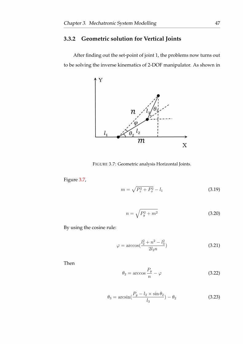
3.3.2 Geometric solution for Vertical Joints
After finding out the set-point of joint 1, the problems now turns out
to be solving the inverse kinematics of 2-DOF manipulator. As shown in
FIGURE 3.7: Geometric analysis Horizontal Joints.
Figure 3.7,
m =√P 2z + P 2
x − l1 (3.19)
n =√P 2y +m2 (3.20)
By using the cosine rule:
ϕ = arccos(l22 + n2 − l23
2l2n) (3.21)
Then
θ2 = arccosPyn− ϕ (3.22)
θ3 = arcsin(Py − l2 × sin θ2
l3)− θ2 (3.23)
Page 48
Chapter 3. Mechatronic System Modelling 48
The inverse kinematic above is only working on the upper half plant (y ≥
0), when working in the other half, let
θ2 = arccosPyn
+ ϕ (3.24)
θ3 = arcsin(Py − l2 × sin θ2
l3) (3.25)
As shown in Figure 3.8, the multiple solutions exist not only in the
angles but also in the pose choosing. The pose problems may be solved
FIGURE 3.8: Geometric analysis Vertical Joints.
by trajectory optimisation. In some cases, the physical structure of the
manipulator may also constrain the other possible poses.
Page 49
Chapter 3. Mechatronic System Modelling 49
3.4 Controller Design
The dynamics of n-DOF manipulator is
θ = M(θ)−1(τ − V (θ, θ)−G(θ)). (3.26)
In the simulation, an alternative control signal ui is used to represent the
coupled input torque. After having the proper control signal design, in-
verse kinematic is used to decouple the torques. Let
x = θ, (3.27)
where [x1 x2 x3]T = [θ1 θ2 θ3]T and [x4 x5 x6]T = [θ1 θ2 θ3]T .
3.4.1 Feedback Linearisation for Manipulator Modelling
From Equation (3.26), the manipulator dynamics has strong non-
linearity with coupled inputs, which can be represented by a general
nonlinear expression,
x = f(x) + g(x)τ, (3.28)
where x = θ, f(x) = M(θ)−1(−V (θ, θ) − G(θ)), g(x) = M(θ)−1. Then an
alternative control signal vector u is used to take place of system input,
x = f(x) + u, (3.29)
where
u =
[0 0 0 u1 u2 u3
]T= g(x)τ. (3.30)
Page 50
Chapter 3. Mechatronic System Modelling 50
Then if the alternative input u is picked in a certain way, it is possible to
transfer the nonlinear dynamics into linear. Pick
ui = −fi(x) + vi, (3.31)
where vi represents the control signal needed to be designed. Then the
nonlinear system turns into linear system,
x =
[x4 x5 x6 v1 v2 v3
]T(3.32)
The system shown above can be divided into three simple linear systems,
each of which represents one of the basic physical definitions. However,
basing on the expression of ui, it is not hard to notice these three subsys-
tems are not independent.
FIGURE 3.9: Linear Close-loop Subsystem.
3.4.2 Ackerman Controller
In this system, Ackerman method is chosen as the method in con-
troller design. Before designing the controller, the controllability of the
Page 51
Chapter 3. Mechatronic System Modelling 51
system needs to be checked.
Qc =
[B AB
]=
0 1
1 0
(3.33)
rank[Qc] = 2 (3.34)
The controllable matrix is full rank, so the linear system is controllable.
To make the system stable, move the poles to −1 ± j, the characteristic
polynomials are
(λ+ 1− j)(λ+ 1 + j) = λ2 − 2λ+ 2 (3.35)
λ(A) = A2 + 2A+ 2I (3.36)
K = [0 1]Q−1λ(A) (3.37)
K =
[2 2
](3.38)
The controller is
ui = −fi(x)−Kx (3.39)
From the simulation result, the system has been settled and the static
error goes to zero.
Page 52
Chapter 3. Mechatronic System Modelling 52
3.4.3 System State Observer Design
Observability
In the practical industrial processes, some of the states cannot be re-
flected directly by the output; moreover, some are even hard to be de-
tected by other methods. But in the controller these states are needed,
so it is necessary to design an observer to observe these states for the
controller designing.
Before design the observers, the system must be observable. But in
some special cases, if the unobservable parts are asymptotically stable, it
is still possible to design the observer for the system. For the system
x = Ax+Bu
y = Cx
(3.40)
If the system is observable, the system must satisfies the following con-
straints
V =
C
CA
...
CAn−1
(3.41)
rank(V ) = n (3.42)
For the subsystems in the dynamics
A =
0 1
0 0
C =
[1 0
](3.43)
Page 53
Chapter 3. Mechatronic System Modelling 53
rank(V ) = 2 (3.44)
Then the system is observable.
Full-Order Observer Design
The full-order observer is a restructuring system basing on the sys-
tem dynamics. As shown in Figure 5.1, a feedback L(y − Cx) is brought
in to cancel the perturbation of the system dynamics. The observer can
FIGURE 3.10: Full-Order Observer.
be represented as:
˙x = (A− LC)x+ Ly +Bu
x(0) = x0
y = Cx
(3.45)
Page 54
Chapter 3. Mechatronic System Modelling 54
For the manipulator dynamics,
A =
0 1
0 0
B =
0
1
C =
[1 0
](3.46)
The dual coefficient matrix is:
A = AT , B = CT (3.47)
Design the poles of the observer located at λ∗1,2 = −5
λi(A− BK) = λ∗i (3.48)
The state feedback matrix K is
K =
[10 25
](3.49)
Let
L = KT (3.50)
Then
A− LC =
−10 1
−25 0
(3.51)
The full-order observer is
˙x =
−10 1
−25 0
x+
0
1
u+
10
25
x1 (3.52)
Page 55
Chapter 3. Mechatronic System Modelling 55
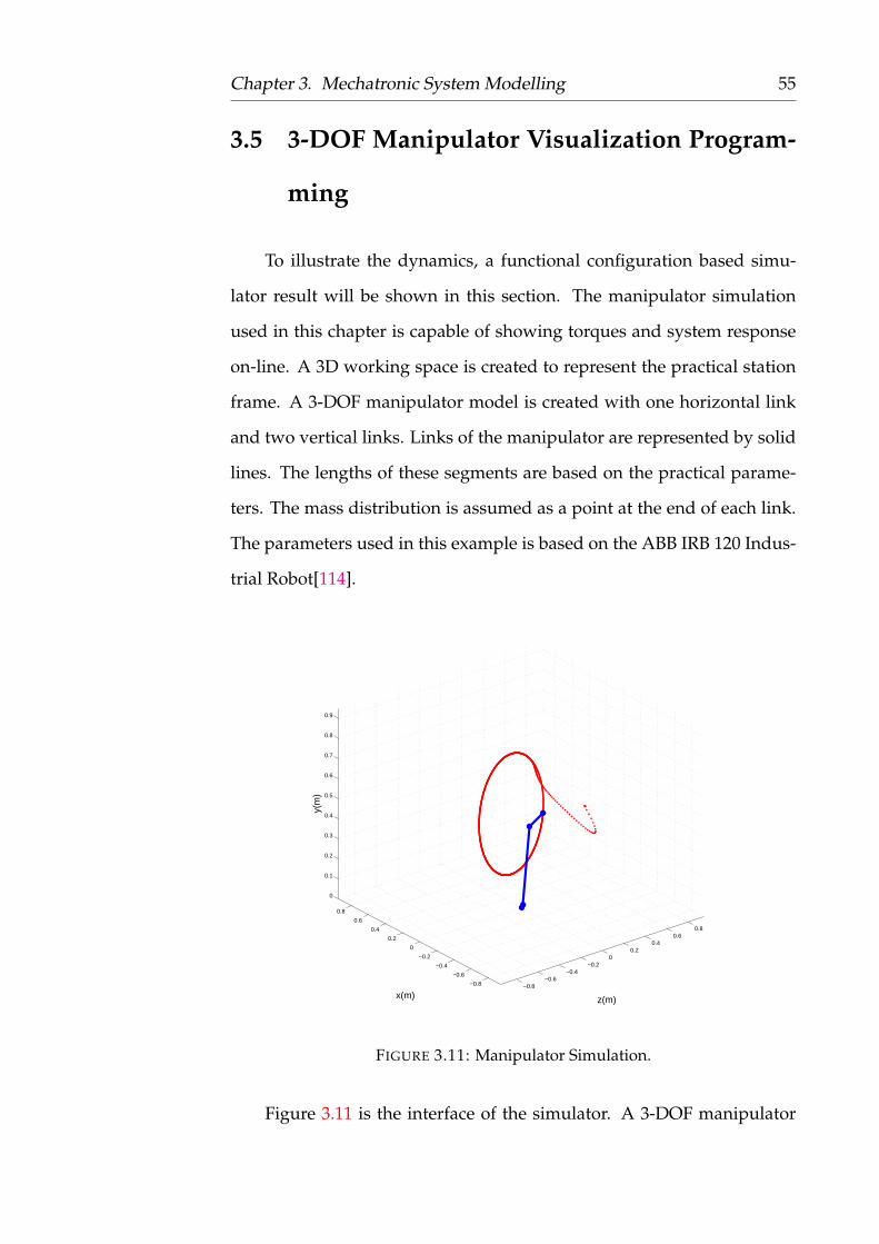
3.5 3-DOF Manipulator Visualization Program-
ming
To illustrate the dynamics, a functional configuration based simu-
lator result will be shown in this section. The manipulator simulation
used in this chapter is capable of showing torques and system response
on-line. A 3D working space is created to represent the practical station
frame. A 3-DOF manipulator model is created with one horizontal link
and two vertical links. Links of the manipulator are represented by solid
lines. The lengths of these segments are based on the practical parame-
ters. The mass distribution is assumed as a point at the end of each link.
The parameters used in this example is based on the ABB IRB 120 Indus-
trial Robot[114].
−0.8−0.6
−0.4−0.2
00.2
0.40.6
0.8
−0.8
−0.6
−0.4
−0.2
0
0.2
0.4
0.6
0.8
0
0.1
0.2
0.3
0.4
0.5
0.6
0.7
0.8
0.9
y(m
)
z(m)x(m)
FIGURE 3.11: Manipulator Simulation.
Figure 3.11 is the interface of the simulator. A 3-DOF manipulator
Page 56
Chapter 3. Mechatronic System Modelling 56
model is displayed to demonstrate the pose of manipulator on-line. The
trajectory of the manipulator is marked by dashed line.
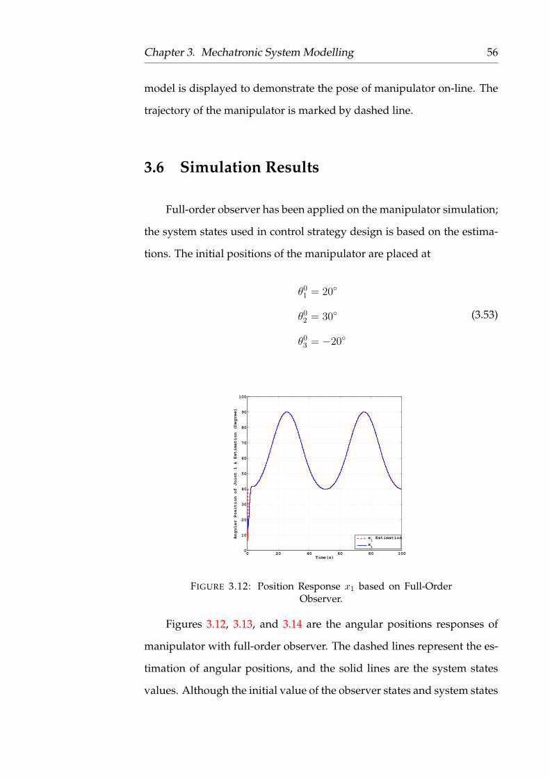
3.6 Simulation Results
Full-order observer has been applied on the manipulator simulation;
the system states used in control strategy design is based on the estima-
tions. The initial positions of the manipulator are placed at
θ01 = 20◦
θ02 = 30◦
θ03 = −20◦
(3.53)
0 20 40 60 80 1000
10
20
30
40
50
60
70
80
90
100
Time(s)
Angular Position of Joint 1 & Estimation (Degree)
x1 Estimation
x1
FIGURE 3.12: Position Response x1 based on Full-OrderObserver.
Figures 3.12, 3.13, and 3.14 are the angular positions responses of
manipulator with full-order observer. The dashed lines represent the es-
timation of angular positions, and the solid lines are the system states
values. Although the initial value of the observer states and system states
Page 57
Chapter 3. Mechatronic System Modelling 57
0 20 40 60 80 1000
10
20
30
40
50
60
70
80
90
100
Time(s)
Angular Position of Joint 2 & Estimation (Degree)
x2 Estimation
x2
FIGURE 3.13: Position Response x2 based on Full-OrderObserver.
0 20 40 60 80 100−120
−100
−80
−60
−40
−20
0
Time(s)
An
gu
lar
Po
sitio
n o
f Jo
int
3 &
Est
ima
tion
(D
eg
ree
)
x3 Estimation
x3
FIGURE 3.14: Position Response x3 based on Full-OrderObserver.
are different, the states observer need few seconds to converge to the tar-
get value. The difference between also makes the gain in the observer
loop higher than that in the control loop, which introduces the oscillation
at the beginning of the process.
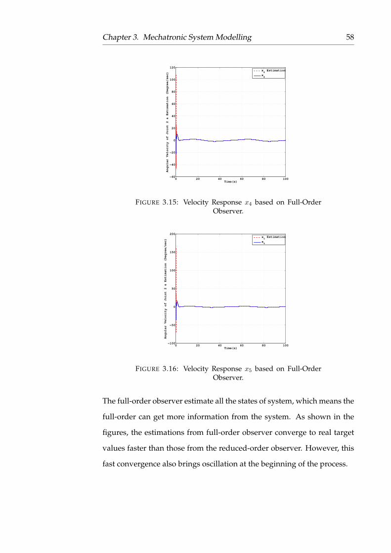
Figures 3.15, 3.16, and 3.17 are the angular velocity responses of the
system with full-order observer. The dashed lines are the estimations of
angular velocities, and the solid lines are the system angular velocities.
Page 58
Chapter 3. Mechatronic System Modelling 58
0 20 40 60 80 100−60
−40
−20
0
20
40
60
80
100
120
Time(s)
An
gu
lar
Ve
loci
ty o
f Jo
int
2 &
Est
ima
tion
(D
eg
ree
/se
c)
x4 Estimation
x4
FIGURE 3.15: Velocity Response x4 based on Full-OrderObserver.
0 20 40 60 80 100−100
−50
0
50
100
150
200
Time(s)
An
gu
lar
Ve
loci
ty o
f Jo
int
2 &
Est
ima
tion
(D
eg
ree
/se
c)
x5 Estimation
x5
FIGURE 3.16: Velocity Response x5 based on Full-OrderObserver.
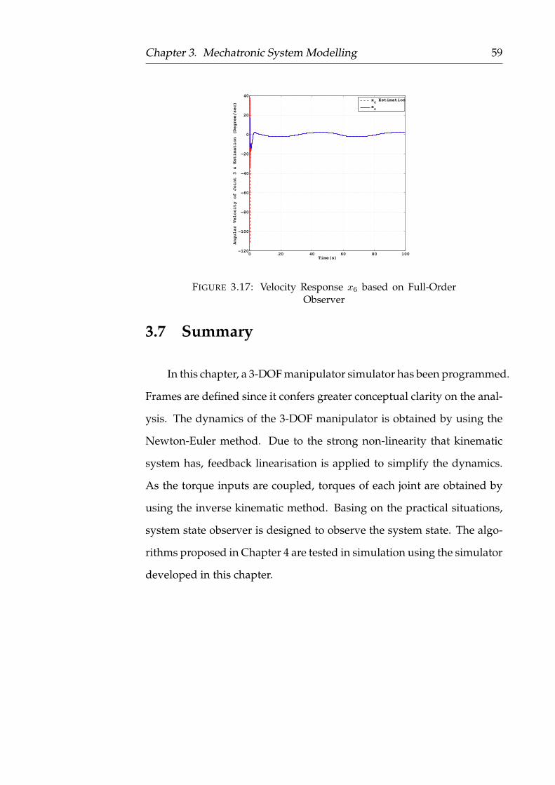
The full-order observer estimate all the states of system, which means the
full-order can get more information from the system. As shown in the
figures, the estimations from full-order observer converge to real target
values faster than those from the reduced-order observer. However, this
fast convergence also brings oscillation at the beginning of the process.
Page 59
Chapter 3. Mechatronic System Modelling 59
0 20 40 60 80 100−120
−100
−80
−60
−40
−20
0
20
40
Time(s)
An
gu
lar
Ve
loci
ty o
f Jo
int
3 &
Est
ima
tion
(D
eg
ree
/se
c)
x6 Estimation
x6
FIGURE 3.17: Velocity Response x6 based on Full-OrderObserver
3.7 Summary
In this chapter, a 3-DOF manipulator simulator has been programmed.
Frames are defined since it confers greater conceptual clarity on the anal-
ysis. The dynamics of the 3-DOF manipulator is obtained by using the
Newton-Euler method. Due to the strong non-linearity that kinematic
system has, feedback linearisation is applied to simplify the dynamics.
As the torque inputs are coupled, torques of each joint are obtained by
using the inverse kinematic method. Basing on the practical situations,
system state observer is designed to observe the system state. The algo-
rithms proposed in Chapter 4 are tested in simulation using the simulator
developed in this chapter.
Page 60
60
Chapter 4
Fault Matrix based Fault Tolerant
Control
With the increasing ageing and environmental damages, such as ex-
treme temperature, humidity, acidic, dynamics may not be accurate in
few months. Inaccurate dynamics may also be caused by actuator faults
or disturbance. When actuator fault is coupled with disturbance, the cur-
rent fault tolerant strategy may not work well anymore. so it is necessary
to find a method that can not only estimate actuator fault but also isolate
the actuator fault from disturbance.
4.1 Problem Formulation
The mechatronic system dynamics can be written as,
x = Ax+ F (x) + EgΘu+ E∆d(t)
y = Cx
(4.1)
where x =
[x1 x2
]Trepresents the system state vector. x1 ∈ Rn repre-
sents the position vector in mechatronic system, and x2 ∈ Rn is the speed
Page 61
Chapter 4. Fault Matrix based Fault Tolerant Control 61
vector. A =
0 I
0 0
is the coefficient of linear part. F (x) =
[0 f1
]Tis the
nonlinear part of the system. E =
[0 Es
]Tis the new coefficient matrix
with Es = I .
F ∈ Rn is the vector representing both the linear and the nonlinear
parts in the system which satisfies Lipschitz condition, |f(a) − f(b)| ≤
δf |a − b|. E ∈ Rn×n is a coefficient matrix. g ∈ Rm×m represents the non-
linearities between control input and system, which also satisfies |g(a)−
g(b)| ≤ δg|a−b|. Θ ∈ Rm×m is fault matrix with a prior knowledge . u ∈ Rm
is the control input vector. y is the system output. ∆d represents the un-
modelled parts in the system, and is bounded by |∆d| < δd. To make the
system more practical, let us assume that system input is bounded, which
means |Θu| < δu.
The disturbance is generated by a linear exogenous system
ζ = Aoζ
∆d = Dζ
(4.2)
where ζ ∈ Rn×n, ∆ ∈ Rn. The system can be written in a form suitable for
control strategy design. We need to transfer the system into error model.
As a pre-phase work for that, let us define
e1 = x1 − xd
e2 = e1
(4.3)
Page 62
Chapter 4. Fault Matrix based Fault Tolerant Control 62
then the system can be re-written as
e = Ae+ F + EgΘu+ E∆d(t)− Exd
y = C(e+ [xd xd]T )
(4.4)
If the strategy described in this paper is designed properly, both e1 and
e2 should converge to zero at the end, which means the system state x1
achieves the reference vector xd, and x2 guarantees that x1 stays with the
reference.
4.2 Terminal Sliding Mode Controller Design
In this section, a terminal sliding mode controller is proposed for
non-faulty system. Fault matrix is assumed to be constant Θ = I , where
I is an identity matrix.
Lemma 1 ([115]). If there exists a continuous radially unbounded function V :
Rn → R+ ∪ {0} such that 1) V (x) = 0 ⇒ x ∈ M ;2) any solution x(t) of
x = g(t, x), x(0) = x0 satisfies the inequality DV (x(t)) ≤ −(αV p(x(t)) +
βV q(x(t)))k for some α, β, q, p, k > 0, pk < 1, qk > 1, then the set M ⊂ Rn is
globally fixed-time attractive for the system x = g(t, x), x(0) = x0. and
T (x0) ≤ 1
αk(1− pk)+
1
βk(qk − 1),∀x0 ∈ Rn.
Based on the Lemma above, the sliding mode manifold can be ex-
pressed as
S =
e1,1 + α1,1e
γ1,11,1 + α2,1e
γ2,12,1
...
e1,n + α1,neγ1,n1,n + α2,ne
γ2,n2,n
, (4.5)
Page 63
Chapter 4. Fault Matrix based Fault Tolerant Control 63
where ei,j represents the jth element in ei. To make the sliding manifold
applicable to Lemma 1, pick αi > 0, βi > 0. Integers γ1 and γ2 satisfy
γ1 = 2n1−12n1−1
∈ (2,∞), and γ2 = 2n2−12m2−1
∈ (1, 2).
Remark 3. The manifold can transfer to e2 = −( 1α2e1 + α1
α2eγ11 )
1γ2 , which con-
tains two components e1γ21 and e
γ1γ21 . As γ1 ∈ (2,∞) and γ2 ∈ (1, 2), γ1
γ2∈ (1,∞)
and 1γ2∈ (0, 1), it means e
1γ21 can guarantee the fast convergence when |e1| < 1,
and eγ1γ21 guarantees the fast convergence when |e1| ≥ 1.
Dynamics on Manifold for Non-faulty System
The control law requires s = 0 [116],
si =e1,n + α1,nd
dt(eγ1,n1,n ) + α2,n
d
dt(eγ2,n2,n )
=e2,i + α1,iγ1,ieγ1,i−11,i e2,i + α2,iγ2,ie
γ2,i−12,i (fi
+ Es,igiui − xd,i)
=e2,i + α1,iγ1,ieγ1,i−11,i e2,i + α2,iγ2,ie
γ2,i−12,i f
+ α2,iγ2,ieγ2,i−12,i Es,igiui − α2,iγ2,ie
γ2,i−12,i xd,i
=0,
(4.6)
where i = 1, 2, ..., n. From Equation (4.6), the control efforts can be ex-
pressed as,
u∗i =− (α2,iγ2,iEs,igi)−1(e
2−γ2,i2,i + α1,iγ1,ie
γ1,i−11,i e
2−γ2,i2,i
+ α2,iγ2,if − α2,iγ2,ixd,i),
(4.7)
Page 64
Chapter 4. Fault Matrix based Fault Tolerant Control 64
Dynamics outside Manifold for Non-faulty System
Similar to the method described in [25], when the initial condition is
not on the manifold, it is necessary to design an additional part of con-
troller to pull the state towards manifold. Similar to the sliding manifold,
this additional part is structured as
u∗∗i = −(α2,iγ2,ieγ2,i−12,i Es,igi)
−1(β1,isξ1,ii + β2,is
ξ2,ii ), (4.8)
where β1,i and β2,i are positive constants, ξ1,i = 2n2−12m2−1
, ξ1,i = 2p2−12q2−1
,m2, n2, p2,
and q2 ∈ Z+. ξ1,i ∈ (0, 1) and ξ2,i > 1
Singular Problem
Due to the non-linearities of the sliding manifold, singular problem
should be taken into consideration. During the design of the dynamics
outside manifold, e1−γ2,i2,i appears in the controller. In addition, the range
of γ2,i ∈ (1, 2), which means e2,i = 0 is the singular point of the controller.
The singular problem is solved by introducing sinusoidal function as
µi =
sin(π
2
eγ2,i−1
2,i
τ) if e
γ2,i−12,i < τ
1 otherwise
(4.9)
By introducing the sinusoidal function designed above into the controller,
ui =− (α2,iγ2,iEs,igi)−1(e
2−γ2,i2,i + α1,iγ1,ie
γ1,i−11,i e
2−γ2,i2,i
+ α2,iγ2,if − α2,iγ2,ixd,i)−
µi(α2,iγ2,ieγ2,i−12,i Es,igi)
−1(β1,isξ1,ii + β2,is
ξ2,ii ),
(4.10)
Page 65
Chapter 4. Fault Matrix based Fault Tolerant Control 65
To check the stability of the sliding mode controller, choose the Lyapunov
candidate in the form as,
V =1
2s2i (4.11)
where si is the ith manifold. The derivative of the candidate is
V =sisi
=si(e2,i + α1,iγ1,ieγ1,i−11,i e2,i + α2,iγ2,ie
γ2,i−12,i (fi
+ Es,igiui))
=− µi(β1,isξ1,i+1i + β2,is
ξ2,i+1i )
<0.
(4.12)
Based on the expression of the sliding manifold, V = 0 only when e = 0.
Due to the singular problem, the system convergence time can be roughly
estimated by duplicating the conclusion of Lemma 1.
4.3 Observer Design
Uncertainties can be caused by many different reasons, such as ag-
ing, the unmeasured components, working environment changing. In
the controller design, robustness is always in the list of the considera-
tions.
4.3.1 Disturbance Observer
The uncertainties in nonlinear systems always increase the difficulty
level of controller design. In this paper, uncertainties bring chattering
into the sliding mode controller, but if the values of uncertainties can be
Page 66
Chapter 4. Fault Matrix based Fault Tolerant Control 66
estimated, the chattering is easy to deal with. In this section, a distur-
bance observer is used to achieve the dynamics of uncertainties. Moti-
vated by [117], the disturbance observer is suggested as
σ = (Ao − l(e)ED)σ + Aop(e)− l(e)(EDp(e)
+f(e) + Eg(e)Θu− Exd)
ζ = σ + p(e)
∆d = Dζ
, (4.13)
where l(e) is the gain function, p(e) is the nonlinear function to be de-
signed.
The nonlinear variable p(e) is picked as
p(e) = KLr−1f (Ce+ [xd xd]
T ) (4.14)
where r is the relative degree. The observer gain l(e) can be determined
by
l(e) = K∂Lr−1
f (Ce+ [xd xd]T )
∂e(4.15)
4.3.2 Fault Matrix Observer
In this section, an observer-based fault detection strategy is proposed
for the uncertain nonlinear system with both actuator and sensor faults.
Due to the existent of sensor fault, system states cannot be used in the
strategy design. As a result of actuator fault, fault matrix will no longer
be the same as its prior knowledge, which means
Θ = Constant 6= ΘH ,
Page 67
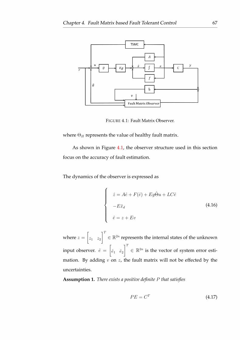
Chapter 4. Fault Matrix based Fault Tolerant Control 67
FIGURE 4.1: Fault Matrix Observer.
where ΘH represents the value of healthy fault matrix.
As shown in Figure 4.1, the observer structure used in this section
focus on the accuracy of fault estimation.
The dynamics of the observer is expressed as
z = Ae+ F (e) + EgΘu+ LCe
−Exd
e = z + Ev
(4.16)
where z =
[z1 z2
]T∈ R2n represents the internal states of the unknown
input observer. e =
[e1 e2
]T∈ R2n is the vector of system error esti-
mation. By adding v on z, the fault matrix will not be effected by the
uncertainties.
Assumption 1. There exists a positive definite P that satisfies
PE = CT (4.17)
Page 68
Chapter 4. Fault Matrix based Fault Tolerant Control 68
To make sure that the estimation will approach the real value of fault
matrix, stability is necessary to be checked. Choose the Lyapunov candi-
date as
V =1
2eTP e+
1
2tr(ΘT Θ) (4.18)
where e = e− e and Θ = Θ− Θ
The derivative of candidate
V =eTP ˙e+ tr(ΘT ˙Θ)
=eTP (Ae+ EgΘu− EgΘu− LCe
+ E∆d − Ev + F − F ) +m∑i=1
θi˙θi
≤− eT (PLC − PA− 1
2P TP − 1
2δ2fI
− 1
2PEETP − 1
2δ2uδ
2gI)e+ eTPET (∆d − v)
+m∑i=1
(ui
m∑j=1
(Ce)j gji + ˙θi)θi
(4.19)
From the expression above, the updating law of Θ is
˙Θ =
u1
m∑j=1
((Ce)j gj1) . . . 0
0. . . 0
0 . . . umm∑j=1
((Ce)j gjm)
(4.20)
The estimation of the disturbance is represented by ∆d. By choosing
v = ∆d (4.21)
Page 69
Chapter 4. Fault Matrix based Fault Tolerant Control 69
the derivative of candidate becomes
V ≤− eT (PLC − PA− 1
2P TP − 1
2δ2fI
− 1
2PEETP − 1
2δ2uδ
2gI)e
(4.22)
If there exists a P that guarantees that (PLC − PA − 12P TP − 1
2δ2fI −
12PEETP
− 12δ2uδ
2gI) ≺ 0, then the fault matrix estimation will be achieved asymp-
totically.
4.4 Fault Tolerant Controller Design
Uncertainties always bring chattering into sliding mode controller.
Those chattering may be caused by the delay of the system and inaccu-
rate system model. To make the uncertainties become an available signal,
disturbance observer is applied here to estimate the value of the uncer-
tainties. By applying multi-layer structure, the inner loop focus on the
stability of system. Disturbance observer is added on outer loop to mon-
itor uncertainties and feedback to the inner loop so that the uncertainties
can be eliminated. But if there is any error between disturbance and its
estimation, then chattering will not be totally eliminated.
Combining Equations (4.10), (4.21), and (4.20), the chattering-reduced
TSMC expression is
u∗i =− (α2,iγ2,iEs,igi)−1(e
2−γ2,i2,i + α1,iγ1,ie
γ1,i−11,i e
2−γ2,i2,i
+ α2,iγ2,if)− (α2,iγ2,ieγ2,i−12,i Es,igi)
−1µi(β1,isξ1,ii
+ β2,isξ2,ii )− (gi)
−1∆d,i + (Es,igi)−1xd,i.
(4.23)
Page 70
Chapter 4. Fault Matrix based Fault Tolerant Control 70
Based on the results above, both the fault matrix and disturbance
can be achieved, it is possible to design a fault tolerant control strategy to
improve the performance when faults occur. To eliminate the effect from
fault matrix, design the control signal as
u = Θ−1u∗ (4.24)
where Θ is the estimation of fault matrix.
The fault tolerant controller is
ui =− (α2,iγ2,iEs,igiθi)−1(e
2−γ2,i2,i + α1,iγ1,ie
γ1,i−11,i e
2−γ2,i2,i
+ α2,iγ2,if)− (α2,iγ2,ieγ2,i−12,i Es,igiθi)
−1µi(β1,isξ1,ii
+ β2,isξ2,ii )− (giθi)
−1∆d,i + (Es,igiθi)−1xd,i.
(4.25)
To check the stability of the system, choose the Lyapunov candidate as
Vi =1
2s2i . (4.26)
The derivative of the candidate is
Vi =sisi
=si[e2,i + α1,iγ1,ieγ1,i−11,i e2,i + α2,iγ2,ie
γ2,i−12,i (fi
+ Es,igiθiui − xd,i + Es∆d)]
=si[e2,i + α1,iγ1,ieγ1,i−11,i e2,i + α2,iγ2,ie
γ2,i−12,i (fi
+ Es,igiθi
θiu∗i − xd,i + Es∆d)]
. (4.27)
As proved above, when the fault happens, Θ → Θ which means Θ
Θ→ I .
The candidate derivative changes into
Page 71
Chapter 4. Fault Matrix based Fault Tolerant Control 71
Vi =sisi
=si[e2,i + α1,iγ1,ieγ1,i−11,i e2,i + α2,iγ2,ie
γ2,i−12,i (fi
+ Es,igiu∗i − xd,i + Es∆d)]
=− µi(β1,isξ1,i+1i + β2,is
ξ2,i+1i )
≤0.
(4.28)
From the proof above, the effect from the fault matrix can be eliminated
by introducing of the FD strategy, and the system remained stable.
4.5 Simulation Result
In order to illustrate the theoretical method proposed in this chapter,
the simulator developed will be used in Chapter 3. The system dynamics
can be written as,
x = Ax+ Eg(x)Θu+ E∆d, (4.29)
where x ∈ R2 is the system state vector, E is the conscience representing
the coupling of disturbance and system input. Θ is fault matrix.u and ∆d
are the system input and disturbance. The system parameters are picked
as
A =
0 1
1 0
E =
0
1
g = 0.5 sin(x1) + 1. (4.30)
When no fault occurs, the fault matrix remains a constant value, let us
assume
ΘH = I. (4.31)
Page 72
Chapter 4. Fault Matrix based Fault Tolerant Control 72
The disturbance in the system is generated by the function
ζ = Aoζ
∆d = Dζ
, (4.32)
where Ao =
0 −0.1
0.1 0
and D =
[0.5 0.5
], which introduces a cosine
disturbance into the system.
The sliding manifold can be written as
s = e1 + 0.2e23111 + 10e
752 , (4.33)
where e = x − [xd xd]. To satisfy the condition described in Equation
(4.12), the controller parameters are picked as
β1
β2
=
0.7
11
ξ1
ξ2
=
137
1115
. (4.34)
To solve the singular problem, µ is picked as
µi =
sin(π
2
e252
τ) if e
252 < 0.01
1 otherwise
. (4.35)
Based on the system dynamics, the disturbance observer gain K =
[5 0.5]. Then the nonlinear variable is determined by
l =
0 5
0 0.5
. (4.36)
Page 73
Chapter 4. Fault Matrix based Fault Tolerant Control 73
In the FTC strategy design, let’s pick
P =
1 2
2 3
L =
2
0.3
. (4.37)
the eigenvalues of PLC − PA − 12PP − 2I − 1
2PEETP are −3.3133 and
−0.2867. The update law of Θ is designed as
˙θ = [0.5 sin(x1) + 1]u(2x1 + 3x2). (4.38)
0 10 20 30 40 50 60 70 80−1
−0.5
0
0.5
1
1.5
2
2.5
Time(s)
Sys
tem
Sta
te
x1 &
Est
ima
tion
(m
)
x1
x1 Estimation
r
FIGURE 4.2: System State (x1) Estimation.
Figure 4.2 is the position response(x1) and its estimation. The thick
dashed curve are the position error estimation, solid curve is the position
feedback. The thin dashed line is the reference signal. Due to the different
initial values system and estimator, the estimation error which is feed
back to observer is big, that makes the estimation increase rapidly. As
Page 74
Chapter 4. Fault Matrix based Fault Tolerant Control 74
the both system dynamics and observer are in continuous time domain,
it needs a period to decrease the feed-back gain after estimation converge
to the system state, which causes the oscillation at the beginning of this
process. When reference changes to 2, there is an error between x1 and
its estimation, which can be caused by the estimation from x2.
0 10 20 30 40 50 60 70 80−0.2
0
0.2
0.4
0.6
0.8
1
1.2
Time(s)
Ve
loci
ty x
2 &
Esi
tma
tion
(m
/s)
x2
x2 Estimation
FIGURE 4.3: System State (x2) Estimation.
Figure 4.3 is the velocity response(x2) of the system, which can be
considered as the changeing rate of x1. The dashed curve is the velocity
estimation, and solid curve is the system velocity As the initial value of
estimator is closer to the reference, the speed of system is faster than that
of estimator. When the estimation of x1 converge to its target state, the
estimation of x2 still above zero, which makes the estimation of x1 keep
increasing When the reference changes to 2, there is a depression in x2,
which is caused by the trigonometric function used in singular problem.
Page 75
Chapter 4. Fault Matrix based Fault Tolerant Control 75
However, the observer is based on the system output and estimation er-
ror, which makes the estimation of x2 smooth.
0 10 20 30 40 50 60 70 80
0.8
1
1.2
1.4
1.6
1.8
2
Time(s)
Fault Matrix & Estimation
ΘΘ Estimation
FIGURE 4.4: Fault Matrix Estimation.
As shown in Figure 4.4, there is no actuator fault existing in the sys-
tem at the beginning of this simulation. Dashed curve is the estimation
from fault observer, and the solid curve is the value of the fault matrix
in the system. The initial values are placed differently from fault initial
matrix value, which cause the oscillation at the beginning. However, as
those target signals working on the system remain the same, x2 has an
overshoot at the beginning. After a short period, as the observer is get-
ting a better estimation, x2 comes back to normal.
In the second half of the process, the fault is set to the value 1.2; the
reference signal value is 2. At the beginning of the second half process,
fault matrix is underestimated for a short time, which makes Θ has an
Page 76
Chapter 4. Fault Matrix based Fault Tolerant Control 76
overshoot. When Θ has overshoot, has overshoot, the system has inade-
quate control, which is shown in the curve of x2.
0 10 20 30 40 50 60 70 80−1
−0.5
0
0.5
1
1.5
2
2.5
3
Time(s)
Dis
turb
an
ce &
Est
ima
tion
DisturbanceEstimation
FIGURE 4.5: Disturbance Estimation.
Figure 4.5 is the result from disturbance observer. Solid curve is the
disturbance generated by exogenous system, and dashed curve is the es-
timation from disturbance observer. As the big initial error from distur-
bance observer, there is an overshoot at the beginning. After the observer
states catch the system states, the disturbance can be observed accurately.
When reference changes to 2, there is only a small overshoot in the dis-
turbance estimation.
Page 77
Chapter 4. Fault Matrix based Fault Tolerant Control 77
4.6 Summary
In this chapter, a fault matrix based fault tolerant control strategy
is proposed. System considered in this chapter is nonlinear and satis-
fies Lipschitz condition. To guarantee the stability of non-faulty system,
terminal sliding mode is used. Different with the conventional sliding
mode control, fixed-time sliding manifold can guarantee system states
converge to zero within fixed-time boundary.
As the existing singular problem, sine function is introduced to guar-
antee the stability of the system. However, as the system states do not en-
force the sliding manifold strictly, the time boundary that calculated may
not guarantee the system converge time any more But as the trigonomet-
ric function only works within a small range, it is possible to add a small
constant in the time boundary to cover the execution time of the trigono-
metric function.
Both disturbance and actuator fault exist in the system. Fault matrix
is used to isolate the actuator fault from disturbance. Moreover, the fault
matrix can also be used to find the relationship between actuator fault
and control signal, which can be used as the coefficient of the controller
to compensate the fault in the system. Disturbance are observed by dis-
turbance observer, the value of disturbance estimation is used to improve
the performance of fault observer.
Page 78
78
Chapter 5
Set-point Re-planning
This chapter proposed a novel set-point re-planning method, which
optimise the deteriorating system performance without changing orig-
inal control loop. As a result of the long maintenance duration of the
manipulator, Robotino mobile robot is used as the experiment platform
for this method.
5.1 Problem Formulation
As most of the industrial processes are controlled by computers, the
signals used in the controller design are discrete.
5.1.1 System Model
The system dynamics considered here can be expressed as,
x1,k+1 = x1,k + hx2,k,
x2,k+1 = x2,k + h(fk + gkuk),
(5.1)
Page 79
Chapter 5. Set-point Re-planning 79
where h is the system sampling time, xi,k = xi(kh), xk =
[x1,k x2,k
]T∈
R2n is the system states vector, fk ∈ Rn represents the nonlinear function
in the system, uk ∈ Rn is the control input vector. gk ∈ Rn is an invertible
matrix that typifies the nonlinear relationships between the control input
uk and system states xk.
In this section, the set-point vector is denoted by r∗ ∈ Rn, and the
system is considered in fault free situation and not affected by distur-
bances. However, the case of systems affected by faults and/or distur-
bances is addressed in section 5.2.1. The errors between system states
and set-point vector can be expressed as,
e1,k = x1,k − r∗k, (5.2)
where r∗k is the set-point vector at time instant k, e1,k ∈ Rn is the vector of
position error at time instant k. Based on relation in Equation (5.2), the
position error at time instant k + 1 can be expressed as
e1,k+1 = x1,k+1 − r∗k+1. (5.3)
Using Equation (5.1), (5.2), and (5.3), the error between two consecu-
tive steps become
e1,k+1 − e1,k = hx2,k − (r∗k+1 − r∗k). (5.4)
In mechatronic systems, and in particular for robotic manipulators, the
set-point for the position of each joint is known and it is given by the
user. There is not any set-point for speeds or accelerations available. In
Page 80
Chapter 5. Set-point Re-planning 80
order to overcome this issue, in this thesis is proposed to be used
e2,k = x2,k −1
h(r∗k+1 − r∗k), (5.5)
where e2 ∈ Rn is the vector of velocity error at time instant k. Based on
Equation (5.1), Equation (5.3) and Equation (5.6),
e1,k+1 = e1,k − h(x2,k −1
h(r∗k+1 − r∗k)), (5.6)
the dynamics for the errors in discrete time become
e1,k+1 =e1,k + he2,k,
e2,k+1 =e2,k + h(fk + gkuk) +1
h(−r∗k+2
+ 2r∗k+1 − r∗k),
(5.7)
In the next paragraph, a SMC for the errors in Equation (5.7) is pro-
posed. The role of the controller is to make the errors to converge at zero
in finite time. This control problem is similar with a trajectory tracking
strategy.
5.1.2 Terminal Sliding Mode
The control method proposed to make the errors from Equation (5.7)
to converge to zero in finite time is terminal sliding mode control. Based
on the contribution made by Man et al. [44], the non-singular sliding
Page 81
Chapter 5. Set-point Re-planning 81
manifold is picked as,
sk =
s1
s2
...
sn
=
e2,1,k + β1eq1p11,1,k
e2,2,k + β2eq2p21,2,k
...
e2,n,k + βneqnpn
1,n,k
, (5.8)
where β ∈ Rn is positive defined. e1,j,k and e2,j,k are the jth component at
time instant k. pi and qi are positive odd integers satisfying qipi∈ (1,∞),
where pi and qi are design parameters. The sliding manifold is a con-
straint to the system states to make the system states to converge to the
origin point following a certain trajectory.
Proposition 1. It is necessary to have qipi∈ (1,∞) so that the sliding manifold
structure choose in (5.8) is a terminal attractor.
Proof. This proof shows x = 0 is an attractor of the sliding manifold.
As discrete time and continuous time are two alternative frame, which
means
e1 = e2 ⇔ e1,k+1 − e1,k. (5.9)
The sliding manifold chosen in Equation (5.8) can be transfer to continu-
ous time frame, which is,
s = e2 + βeqp
1 . (5.10)
When system states are on the manifold,
s = 0. (5.11)
Page 82
Chapter 5. Set-point Re-planning 82
e1 from Equation (5.7) can be expressed in continuous time as,
de1
dt= −βe
qp
1 , (5.12)
then
dt = − 1
βe− qp
1 de1. (5.13)
The convergence time is
t = −e1→0∫e1(0)
1
βe− qp
1 de1
= − 1
β
1
1− qp
e1(0)1− qp
(5.14)
e1(0) is the initial value of e1. The convergence time only meaningful
when t > 0, so qp> 1.
Observation 1. When system states move along the manifold,
si,k+1 = si,k = 0. (5.15)
Then by combining Equation (5.8) and Equation (5.15), the equiva-
lent control law that keeps states on the manifold (5.8) is given by
u∗i,k =− g−1i,k fi,k + g−1
i,k
1
h[βie
qipi1,i,k − βi(e1,i,k
+ he2,i,k)qipi ] + g−1
i,k
1
h2(r∗i,k+2 − 2r∗i,k+1
+ r∗i,k),
(5.16)
where ui,k is the ith control signal at time instant k. However, if the sys-
tem’s initial values are not placed on the manifold (sk = 0), controller
Page 83
Chapter 5. Set-point Re-planning 83
shown in Equation (5.16) cannot transport system states to the sliding
manifold.
To make sure the convergence of the system with initial values out-
side sliding manifold, an additional term need to be added. Based on
[115], the new controller is written as,
ui,k =− g−1i,k fi,k + g−1
i,k
1
h[βie
qipi1,i,k − βi(e1,i,k
+ he2,i,k)qipi ] + g−1
i,k
1
h2(r∗i,k+2 − 2r∗i,k+1
+ r∗i,k)− g−1i,k
1
h(α1,is
n1,im1,i
i,k + α2,is
n2,im2,i
i,k ),
(5.17)
where m1,i,m2,i, n1,i, n2,i are positive odd integers which satisfy n1,i
m1,i∈
(0, 1) and n2,i
m2,i∈ (1,∞). Use the controller described in Equation (5.17)
taking the place of uk in Equation (5.7),
e1,i,k+1 =e1,i,k + he2,i,k,
e2,i,k+1 =e2,i,k + βieqipi1,i,k − βi(e1,i,k + he2,i,k)
qipi
− (α1,is
n1,im1,i
i,k + α2,is
n2,im2,i
i,k ).
(5.18)
To prove the stability of system with the TSMC, the convergence of
the system states has to be checked.
Lemma 2. For the error dynamics shown in Equation (5.7), if the controller is
designed as
ui,k =− g−1i,k fi,k + g−1
i,k
1
h[βie
qipi1,i,k − βi(e1,i,k
+ he2,i,k)qipi ] + g−1
i,k
1
h2(r∗i,k+2 − 2r∗i,k+1
+ r∗i,k)− g−1i,k
1
h(α1,is
n1,im1,i
i,k + α2,is
n2,im2,i
i,k ),
(5.19)
where m1,i,m2,i, n1,i, n2,i are positive odd integers which satisfy n1,i
m1,i∈ (0, 1)
and n2,i
m2,i∈ (1,∞). Then the system state will converge to zero within finite
time.
Page 84
Chapter 5. Set-point Re-planning 84
Proof. By using the sliding manifold described in Equation (5.8), system
states are expected to stay on the manifold (si = 0) after reaching,
si,k+1 = si,k = 0. (5.20)
However, the initial values are not always placed on the sliding man-
ifold. To make the sliding manifold an attractor, it is necessary to prove
that the system states move toward the manifold when they are outside
the sliding manifold (si 6= 0), which means
|si,k+1| < |si,k|. (5.21)
If the convergence of the difference for the surfaces can be proved,
then the stability of the system is guaranteed. The difference between
si,k+1 and si,k is
si,k+1 − si,k
=e2,i,k+1 + βieqipi1,i,k+1 − e2,i,k − βie
qipi1,i,k
=e2,i,k + βieqipi1,i,k − βi(e1,i,k + he2,i,k)
qipi
− (α1,is
n1,im1,i
i,k + α2,is
n2,im2,i
i,k ) + βi(e1,i,k
+ he2,i,k)qipi − e2,i,k − βie
qipi1,i,k
=− (α1,is
n1,im1,i
i,k + α2,is
n2,im2,i
i,k ).
(5.22)
As described above,m1,m2, n1 and n2 are positive odd integer, which
guarantees that the numerator of nimi
+ 1 is even. αj,i is positively defined.
As the convergence of Equation (5.22) is proved in [55], it is obvious to
Page 85
Chapter 5. Set-point Re-planning 85
see |si,k+1| < |si,k|, if |si,k| 6= 0. Then
e2,i,k = −βieq1p11,i,k. (5.23)
The system is globally asymptotically stable. Based on Remark 4, e2,i,k is
a terminal attractor.
However, the same for other practical systems, mechatronic system
is vulnerable to uncertainties. The following method focus on improving
the system performance deteriorated by uncertainties.
5.2 Set-point Re-planning
When uncertainties appear in the system, system performance will
be deteriorated. In this section, a new method of set-point re-planning
is given to control the system even with reduced performances in the
presence of disturbances.
FIGURE 5.1: Block Diagram of Set-point Replanning
Figure 5.1 is the block diagram of set-point replanning. The con-
troller is designed based on the accurate system dynamics. An additive
Page 86
Chapter 5. Set-point Re-planning 86
set-point ∆r is designed to optimise the system performance in presence
of disturbances.
5.2.1 System Model with Disturbance
The system (5.1) can be written in presence of disturbances as in the
following x1,k+1 = x1,k + hx2,k + d1,
x2,k+1 = x2,k + h(fk + gkuk) + d2,
(5.24)
where d1 ∈ Rn and d2 ∈ Rn are the additive uncertainties in the system,
such as any unconsidered signal in the system dynamics. To improve the
system performance, an additional term ∆rζ is used to compensate the
effects of uncertainties. The new reference signal is
rk = ∆rζ + r∗k, (5.25)
where r∗k is the original reference vector. ∆r ∈ Rn is the new compen-
satory set-point to be designed. rk ∈ Rn is the new set-point that used in
the system. (•)ζ shows a different sampling time with the system states
because is computed by the outer loop (see Figure 5.1). As e is used to
represent the error between system states x and the original set-point r∗,
it is necessary to define another error vector for positions that represents
the deference between x and the new set-point r. To avoid confusion in
the notations, the new error vector will be epsilon. Define
ε1,k = x1,k − rk
ε2,k = x2,k − 1h(rk+1 − rk).
, (5.26)
Page 87
Chapter 5. Set-point Re-planning 87
where ε =
[ε1 ε2
]T∈ R2n is the vector representing the error between
system state x and new set-point r. ε1 ∈ Rn and ε2 ∈ Rn. h is the sampling
time. Based on the new vectors defined above, the error dynamics is
ε1,k+1 =ε1,k + hε2,k + d1,
ε2,k+1 =ε2,k + h(fk + gkuk) +1
h(−rk+2
+ 2rk+1 − rk) + d2,
, (5.27)
u is used to represent the controller based on the new error vector. h
is the length of system states sampling time. Similar to the definition
in Equation (5.17), the controller ui,k basing on the new error vector ε is
expressed as,
ui,k =− g−1i,k fi,k + g−1
i,k
1
h[βiε
qipi1,i,k − βi(ε1,i,k
+ hε2,i,k)qipi ] + g−1
i,k
1
h2(r∗i,k+2 − 2r∗i,k+1
+ r∗i,k)− g−1i,k
1
h(α1,is
n1,im1,i
i,k + α2,is
n2,im2,i
i,k ),
(5.28)
where si,k = ε2,i,k + βiεqipi1,i,k is the sliding manifold related to the new
system state vector ε. fi,k = fi(εk) and εj,i,k = εj,i(kh). Combine the
system dynamics described in Equation (5.27) and controller ui,k together,
ε1,k+1 =ε1,k + hε2,k + d1
ε2,k+1 =ε2,k + βεqp
1,k − β(ε1,k + hε2,k)qp + d2
+1
h(−∆rk+2 + ∆2rk+1 −∆rk).
(5.29)
Equation (5.29) is the system dynamics basing on the time-varying set-
point. A novel set-point re-planning method is proposed to improve the
performance of the system expressed in Equation (5.29).
Page 88
Chapter 5. Set-point Re-planning 88
5.2.2 Performance Optimisation
To eliminate the effect of uncertainties, a set-point re-planning method
is proposed. Choose the performance index as [118]
J = eT1,Ne1,N +N−1∑ζ=0
eT1,ζe1,ζ , (5.30)
whereN is the number of sampling points. By choosing this performance
index, system states are expected to stay as close as possible to the set-
point r∗. The outer loop is designed based on this performance index.
Define Hamilton equation [118],
Hζ = eT1,ζe1,ζ + λTζ+1fζ (5.31)
where fζ is the system dynamics, λζ is Hamiltonian. Hamilton equation
is used in the design of outer loop. Based on the chosen performance
index, the Hamiltonian becomes
Hζ =eT1,ζe1,ζ + λTζ+1(ε1,ζ+hε2,ζ+d1
ε2,ζ+h(fζ+gζ uζ)+d2)
=n∑i=1
{ε21,i,ζ + 2ε1,i,ζ∆ri,ζ + ∆2ri,ζ
+ λ1,i,ζ+1(ε1,i,ζ + hε2,i,ζ + d1)
+ λ2,i,ζ+1[ε2,i,ζ + βiεqipi1,i,ζ − βi(ε1,i,ζ
+ hε2,i,ζ)qipi − (α1,is
n1,im1,i
i,ζ + α2,is
n2,im2,i
i,ζ )
− 1
h(∆ri,ζ+2 − 2∆ri,ζ+1 + ∆ri,ζ) + d2]}.
(5.32)
where the λ1 ∈ Rn and λ2 ∈ Rn are the costates, and e1 = ε1 + ∆r.
Remark 4. Because of the sampling time of set-point re-planning loop is bigger
than that of control loop, system state ((•)k) will be sampled multiple times
Page 89
Chapter 5. Set-point Re-planning 89
during one sampling period of re-planned set-point ((•)ζ). In other words, the
re-planned set-point remains the same during each sampling time considering in
Hamilton equation (∆ri,ζ = ∆ri,k+1 = .. 6= ∆ri,ζ+1).
The basic idea of Hamilton equation is to find the minimum value
by using the partial derivative related to the performance index.
λ1,i,ζ =∂Hζ
∂ε1,i,ζ
=λ2,i,ζ+1[βiqipiεqipi−1
1,i,ζ − βiqipi
(ε1,i,ζ
+ hε2,i,ζ)qipi−1 − (α1,i
n1,i
m1,i
s
n1,im1,i−1
i,ζ
+ α2,in2,i
m2,i
s
n2,im2,i−1
i,ζ )βiqipiεqipi−1
1,i,ζ ]
+ 2ε1,i,ζ + 2∆ri,ζ + λ1,i,ζ+1,
λ2,i,ζ =∂Hζ
∂ε2,i,ζ
=λ1,i,ζ+1h+ λ2,i,ζ+1[1− βihqipi
(ε1,i,ζ
+ hε2,i,ζ)qipi−1 − (α1,i
n1
m1
s
n1,im1,i−1
i,ζ
+ α2,in2,i
m2,i
s
n2,im2,i−1
i,ζ )].
(5.33)
As Equation (5.33) has strong non-linearities, singular problem need
to be checked.
5.2.3 Singular Problem
As the component related to sn1,im1,i−1
i,ζ appears in the costate dynamics,
singular problem has to be considered. Meanwhile, n1
m1∈ (0, 1), the sin-
gular problem has to be taken into consideration when ε1 = 0 or when
the system reaches the manifold. To solve the singular problem, a new
Page 90
Chapter 5. Set-point Re-planning 90
coefficient is introduced [119],
µi,ζ =
sin(π
2
|s1−
n1,im1,i
i,ζ |τ
) if |s1−
n1,im1,i
i,ζ | ≤ τ
1 otherwise
, (5.34)
where τ is a small scalar that represents the execution area of the sinu-
soidal function. After introducing the new coefficient, the costates dy-
namics change into
λ1,i,ζ =∂Hζ
∂ε1,i,ζ
=λ2,i,ζ+1[βiqipiεqipi−1
1,i,ζ − βiqipi
(ε1,i,ζ
+ hε2,i,ζ)qipi−1 − (α1,i
n1,i
m1,i
µi,ζ s
n1,im1,i−1
i,ζ
+ α2,in2,i
m2,i
s
n2,im2,i−1
i,ζ )βiqipiεqipi−1
1,i,ζ ]
+ 2ε1,i,ζ + 2∆ri,ζ + λ1,i,ζ+1,
λ2,i,ζ =∂Hζ
∂ε2,i,ζ
=λ2,i,ζ+1[1− βihqipi
(ε1,i,ζ + hε2,i,ζ)qipi−1
− (α1,in1,i
m1,i
µi,ζ s
n1,im1,i−1
i,ζ + α2,in2,i
m2,i
s
n2,im2,i−1
i,ζ )]
+ λ1,i,ζ+1h.
(5.35)
where µi,ζ is added in front of sn1,im1,i−1
i,ζ to solve the singular problem.
To make sure that the re-planned set-point have the extremum, ∆ri has
to satisfies the stationary condition, which is
0 =∂Hζ
∂∆ri,ζ
= 2ε1,i,ζ + 2∆ri,ζ −1
hλ2,i,ζ+1.
(5.36)
Page 91
Chapter 5. Set-point Re-planning 91
The re-planned set-point is
∆ri,ζ = −ε1,i,ζ +1
2hλ2,i,ζ+1, (5.37)
where ∆ri,ζ is the additive set-point on the ith set-point component.
As an additional optimal closed-loop is added, the stability of the
new closed-loop system has to be checked.
Theorem 5.2.1. Suppose that the system (5.7) with the controller shown in
Equation (5.28) is affected by uncertainties denoted by d1 and d2 . Then under
the re-planned set-point ∆rζ , the performance index described as Equation (5.30)
will be optimised, moreover, the system states will track the original set-point r∗.
Proof. Since the set-point update law (Equation (5.37)) is introduced, the
new set-point becomes rζ = r∗ζ + ∆rζ , where ∆rζ has been derived by
Equation (5.37). The feedback errors used in the controller design change
from e to ε. If the convergence of ε to e can be proved, then the system
states will track r∗.
By combining Equation (5.35) and Equation (5.37) together, the costates
relationships become,
λ1,i,ζ+1 =λ1,i,ζ − Aλ2,i,ζ+1,
λ2,i,ζ+1 =λ2,i,ζ − λ1,i,ζ+1h+Bλ2,i,ζ+1,
(5.38)
whereA =
1
h− βi
qipiεqipi−1
1,i,ζ + βiqipi
(ε1,i,ζ + hε2,i,ζ)qipi−1
+ (α1,in1,i
m1,i
µi,ζ s
n1,im1,i−1
i,ζ
+ α2,in2,i
m2,i
s
n2,im2,i−1
i,ζ )βiqipiεqipi−1
1,i,ζ
(5.39)
Page 92
Chapter 5. Set-point Re-planning 92
andB =βih
qipi
(ε1,i,ζ + hε2,i,ζ)qipi−1
+ (α1,in1,i
m1,i
µi,ζ s
n1,im1,i−1
i,ζ + α2,in2,i
m2,i
sn2m2−1
i,ζ ).
(5.40)
If the system has equilibrium points, then system states will remain
at one of them eventually. Assume the system described in Equation
(5.44) has equilibrium points, based on the properties of equilibrium points,
λi,ζ = λi,ζ+1. (5.41)
Combining the relationship between λi,ζ and λi,ζ+1 with Equation (5.44),
0 = Aλ2,i,ζ+1,
0 = −λ1,i,ζ+1h+Bλ2,i,ζ+1.
(5.42)
WhenAλ2,i,ζ+1 = 0, eitherA or λ2,i,ζ+1 should be zero. AssumeA = 0,
1
h=βi
qipiεqipi−1
1,i,ζ − βiqipi
(ε1,i,ζ + hε2,i,ζ)qipi−1 − (α1,i
n1,i
m1,i
µi,ζ s
n1,im1,i−1
i,ζ
+ α2,in2,i
m2,i
s
n2,im2,i−1
i,ζ )βiqipiεqipi−1
1,i,ζ
(5.43)
If |εi,ζ | = 0, equation becomes 1h
= 0, which is impossible. So it is neces-
sary to guarantee |εi,ζ | 6= 0 to compensate 1h
. However, as the convergence
of system states is guaranteed, which shows that |εi,ζ | → 0. As |εi,ζ | → 0,
A does not converge to zero.
Page 93
Chapter 5. Set-point Re-planning 93
Based on Equation (5.44), if let λ2,ζ+1 = 0,
λ1,i,ζ+1 =λ1,i,ζ ,
λ2,i,ζ =λ1,i,ζ+1h,
(5.44)
As the λ2,i,ζ = λ2,i,ζ+1, it is clear that the system will stay at λi,ζ+1 = 0.
When λ1 = λ2 = 0, combine the system dynamics, which is shown
in Equation (5.26), and re-planned set-point in Equation (5.37),
0 =x1,i,ζ − r∗i,ζ ,
0 =x2,i,ζ −1
h(r∗ζ+1 − r∗ζ),
(5.45)
then it is obvious that x→ r∗.
The theorem 5.2.1 proves the set-point replanning not only optimise
the system performance in presence of disturbance, but also guarantee
the system states keep tracking the original set-point r∗ in presence of
disturbances.
5.3 Case-study on Mobile Robot
With increasing interest in industrial automation, mobile robot has
been playing an important role in transportation, rescue, etc.. Mobile
robot always works in complex situations in which uncertainties are in-
evitable. Most of those applications rely on the accurate robot locations
feedback; however, the original controller may not able to guarantee that
accuracy when uncertainties occur.
Mobile robot is used in the experiment. The programming environ-
ment is Ubuntu Linux. Based on the special distribution of three wheels,
Page 94
Chapter 5. Set-point Re-planning 94
FIGURE 5.2: Holonomic Mobile Robot c©Festo Didactic.
TABLE 5.1: Robotino DC Motor Parameters.
DC motor(GR 42x25)Rated Voltage 24VDCRated Speed 3600RPMRated Torque 3.8NcmRated Current 0.9AStarting Torque 20NcmStarting Current 4ANo Load Speed 4200RPMMotor Weight 390g
Robotino is capable of moving omni-directionally. Wheels are driven by
DC motors, whose data specification is shown in Table I.
Figure 5.3 is the block diagram of the basic close-loop design of Robotino.
The trajectory planning agency generates the set-points based on the re-
quirements. The control signals are generated from an external com-
puter. The control signals are passed to Robotino through the inherent
Robotino’s WLAN-Link. The embedded system in Robotino transfers the
velocity setting values into torques. To guarantee the primary stability of
the mobile robot, Robotino has a PI controller inside.
Page 95
Chapter 5. Set-point Re-planning 95
Basing on the structure of sliding manifold shown in Equation (5.8), the
FIGURE 5.3: Block Diagram of Robotino Control.
sliding manifolds used here is
s = v + αpγ, (5.46)
where v represents the velocity os mobile robot, p is the position feedback
from encoder. In this practical test, choose γ = 119
, and α = 2.
The performance index used here is
J = eT1,Ne1,N +N−1∑k=0
eT1,ke1,k. (5.47)
Page 96
Chapter 5. Set-point Re-planning 96
0 50 100 150 200 250 300−1
−0.8
−0.6
−0.4
−0.2
0
Samples(0.03s/sample)
Po
sitio
n E
rro
r e
x(m
)
Sampled Position ErrorPosistion Error
FIGURE 5.4: Position Error in x Direction
0 50 100 150 200 250 300−0.7
−0.6
−0.5
−0.4
−0.3
−0.2
−0.1
0
0.1
0.2
0.3
Samples(0.03s/sample)
Po
sitio
n E
rro
r e
y(m
)
Sampled Position ErrorPosistion Error
FIGURE 5.5: Position Error in y Direction.
Figure 5.4 and Figure 5.5 are the position errors in x and y directions.
Page 97
Chapter 5. Set-point Re-planning 97
Dashed curves are the resampled position errors which are used in the
controller design, and solid curves are the position feedbacks. Uncertain-
ties have been added to the controller inputs. Controller’s inputs affected
by uncertainties are represented by solid curves. The figures also show
that when system works without the optimal loop, the robot’s stability is
still guaranteed. According to the hardware structure and programming
logic, the optimised control signal may not able to follow the system if
their sampling frequencies remain the same. Multi-rate sampling method
is used in the experiment. Dotted curves represent the re-sampled sig-
nals. The new sampling frequency is one tenth of the system’s clock fre-
quency.
0 50 100 150 200 250 3000
0.02
0.04
0.06
0.08
0.1
0.12
0.14
0.16
0.18
0.2
Samples(0.03s/sample)
Linear Velocity vx(m/s)
Sampled System Velocity System Velocity
FIGURE 5.6: Velocity in x Direction.
Page 98
Chapter 5. Set-point Re-planning 98
0 50 100 150 200 250 300−0.05
0
0.05
0.1
0.15
0.2
0.25
0.3
0.35
0.4
Samples(0.03s/sample)
Lin
ea
r V
elo
city
vy(m
/s)
Sampled System Velocity System Velocity
FIGURE 5.7: Velocity in y Direction
Velocities of the mobile in each direction are shown in Figure 5.6 and
5.7. Dashed curves are the resampled velocities going to be used in con-
troller design, and solid curves are the velocity feedbacks. Same as posi-
tions, the re-sampled velocities are shown in dotted curves. At the begin-
ning of process, as the big errors between robot position and set-point,
controller contributes a high gain, which rise the speed rapidly. As the
position errors decrease, the speed decreases smoothly. As the existing
uncertainties, position errors can not converge to zero, and speeds keep
chattering at the end of process.
Page 99
Chapter 5. Set-point Re-planning 99
0 50 100 150 200 250 300−1.2
−1
−0.8
−0.6
−0.4
−0.2
0
0.2
Samples(0.03s/sample)
Slid
ing
Ma
nifo
ld
sx
sx based on Reselected Setpoint
sx
FIGURE 5.8: Sliding Manifold on x Direction (sx).
0 50 100 150 200 250 300−1.2
−1
−0.8
−0.6
−0.4
−0.2
0
0.2
0.4
Samples(0.03s/sample)
Slid
ing
Ma
nifo
ld s
y
sy based on Reselected Setpoint
sy
FIGURE 5.9: Sliding Manifold on y Direction (sy).
Figures 5.8 and 5.9 show the differences of sliding manifolds based
Page 100
Chapter 5. Set-point Re-planning 100
on both r∗ and r. Solid curves are the sliding manifold with original
set-points, and dashed curves are from the system with re-planned set-
point. In Figure 5.8, the re-planned set-points increase the feedback error
at the beginning which offers a faster speed response. In Figure 5.9, the
re-planned set-point not only gives a faster response but also introduces
an overshoot in the sliding manifold in y direction. The difference in
the responses of sliding manifolds in x and y direction is caused by the
mechanical wearing and sensor ageing
0 50 100 150 200 250 300−0.5
−0.45
−0.4
−0.35
−0.3
−0.25
−0.2
−0.15
−0.1
−0.05
0
Samples(0.03s/sample)
Po
sitio
n E
rro
r e
x(m
)
Optimized Position Error Position Error
FIGURE 5.10: Optimal system output error (ex).
Figure 5.10 and Figure 5.11 are the comparisons of optimised and
original position errors. Solid curves are original position feedbacks from
encoders, and dashed curves are the optimised position feedbacks. and
As the larger position errors that the re-planned set-point give, the mobile
robot goes to the target point faster than before. When steady state errors
exist in the system, ∆r also compensates the steady state errors. The
Page 101
Chapter 5. Set-point Re-planning 101
optimisation, the mobile robot not only has a faster response but also an
improved accuracy.
0 50 100 150 200 250 300−0.5
−0.4
−0.3
−0.2
−0.1
0
0.1
0.2
Samples(0.03s/sample)
Po
sitio
n E
rro
rey (
m)
230 240 250
−2
0
2
4
6
x 10−3
Optimized Position Error Position Error
FIGURE 5.11: Optimal system output error (ey).
Page 102
Chapter 5. Set-point Re-planning 102
0 50 100 150 200 250 3000
2
4
6
8
10
12
14
16
18
20
Samples(0.03s/sample)
System Performance Index J(m2)
Optimized System Performance Index
System Performance Index
FIGURE 5.12: System Performance Index.
Figure 5.12 is the performance index of the mobile robot. Solid curve
is the optimised system performance index, and dashed curve are the
original system performance index As the faster response and smaller
system steady state errors, the accumulation of system states with re-
planned set-point is better than that with original set-point.
5.4 Summary
In this chapter, an operational optimal control strategy is designed
for the mechatronic system. Terminal sliding mode control is used to
make the system converge time adjustable.
Different with the conventional optimal control strategy, the strat-
egy proposed optimises the deteriorating system performance without
Page 103
Chapter 5. Set-point Re-planning 103
change the controller parameters. The multi-rate method is used to make
sure that the system states can follow the re-planned set-point.
Hamilton-Jacobin-Bellman(HJB) equation is applied on the outer loop
as the optimal method. However, as the complex structure of the origi-
nal closed loop, the singular problem exists. A trigonometric function is
used to solve the singular problem. The convergence and stability of the
system with the optimal loop is proved in Theorem 5.2.1.
Page 104
104
Chapter 6
Conclusion and Future Work
6.1 Conclusion
In the first part of this thesis, a 3-DOF manipulator dynamics is built
based on the Newton-Euler method. Newton-Euler method is used to
achieved the dynamics. To make the dynamics easier to be tested, a visu-
alized program is designed. The control method used in the simulator is
state-feedback control. To make the simulator more practical, both full-
order and reduced-order observer have been applied to it.
In the second part, a fault matrix based fault tolerant control strategy
is proposed. A terminal sliding mode manifold is used in the controller
design to guarantee the system converge time. However, during the con-
troller design, (eγ2−12 )−1 appears. As γ2 ∈ (1, 2), singular problem has to
be considered. To solve the singular problem, a mathematical approxi-
mation, sin(x)x
= 1 when x → 0, is used. To eliminate the impact of dis-
turbance, a disturbance observer has been applied in the strategy. When
actuator fault exist in the system, fault matrix is used to represent the ac-
tuator fault based on its relationship with the control signal. Because of
the existence of sensor fault, system states cannot be used directly in the
fault tolerant control strategy design.
Page 105
Chapter 6. Conclusion and Future Work 105
As both actuator fault and control signal are related to system state,
fault matrix is used to represent the relationship between them. To esti-
mate the fault matrix, a Luenberger-like fault observer is designed, which
means output error will be used in the design. By using the bounds of
system non-linearities and a time domain disturbance observer, actuator
fault is isolated. Different with the typical target system of observer, fault
matrix is coupled in the middle of other nonlinear parts (EgΘu). Inequal-
ity features are used to uncoupled the fault matrix. A simulation result
has been given in the last section to illustrate the method.
In the third part, a novel set-point re-planning method is proposed.
Robotino mobile robot is chosen as real platform. Similar to FTC, a termi-
nal sliding mode controller is applied on the system to guarantee system
output tracking the desired trajectory. Different with the sliding manifold
used in FTC design, a simpler sliding manifold is used to give controller
better applicability. To make the convergence time controllable, was cho-
sen qipi> 1. The reaching part is still based on the similar structure as
in the fault observer design. As the exponential function takes the place
of sign function, system states converge to set-point smoothly. However,
the robustness of sliding mode control is decreased.
When uncertainties exist in the system, system performance will be
damaged. In conventional optimal control, controller parameters need
to be changed. As the increasing acceptance of industrial automation,
mechatronic systems are provided with embedded controller, which makes
controllers inaccessible. Instead of changing controller parameters, set-
point re-planning method is proposed. Although an additional set-point
(∆r) is added to the system, system states are still expected to tracking the
original set-point (r∗). As the new set-point in the system is (r = ∆r+r∗),
system states error has to be update. Because the target trajectory is r∗,
Page 106
Chapter 6. Conclusion and Future Work 106
system performance chosen here is based on the original error (e = x−r∗).
Hamilton-Jacobi-Bellman equation is used to achieve the update law. The
optimal loop is considered as an outer loop in the control scheme. If the
original control close-loop is considered as a black box, the stability of
optimal loop has to be proved, which is shown in Theorem 5.2.1.
6.2 Thesis Contributions
The contributions of this thesis are:
• Designed a terminal sliding mode controller. Exponential structure
guarantees the global fast convergence. The closed-loop system is
proved to be asymptotically stable. The singular problem in con-
troller design is solved by using mathematical approximation.
• Proposed a fault matrix based fault tolerant control strategy. Actu-
ator faults in the system are represented by using the relationships
between controller and actuator faults. Because disturbance is re-
lated to time, disturbance isolated by using a time relating distur-
bance observer.
• Proposed a set-point re-planning optimal method. Instead of chang-
ing controller parameters, set-point(rk = ∆rζ + r∗k) is used to opti-
mise the system performance. As the re-planned set-point (∆rζ) is
used to compensate the uncertainties, system states is still expected
to track the original set-point(r∗k). The convergence of the system
state is proved.
• Several papers related to the thesis have been published
Page 107
Chapter 6. Conclusion and Future Work 107
• X. Yan, B. Tian and H. Wang, "An adaptive observer-based
fault detection and diagnosis for nonlinear systems with sen-
sor and actuator faults," International Conference on Advanced
Mechatronic Systems (ICAMechS), Beijing, China, 2015, pp. 491-
496.
• X. Yan, Z. Zuo, L. Yin, A. Wang and H. Wang, "Chattering-
free sliding mode control for MIMO nonlinear manipulator
systems based on adaptive neural networks," The 54th IEEE
Conference on Decision and Control (CDC), Osaka, Japan, 2015,
pp. 6300-6305.
• B. Tian, Z. Wang, X. Yan, H. Wang, "Fault-tolerant control scheme
for manipulator with actuator and sensor failure," International
Journal of Advanced Mechatronic Systems 2015, 6(4), pp. 166-173.
• B. Tian, Z. Zuo, X. Yan, H. Wang. "A fixed-time output feed-
back control scheme for double integrator systems," Automat-
ica, 2017, 80, pp. 17-24.
Page 108
Chapter 6. Conclusion and Future Work 108
6.3 Future Work
In the thesis, the set-point re-planning strategy is designed for the
system with certain parameters, however, as loads of many mechatronic
systems, such as those in sorting, medical care, and transporting, are not
constants. It may necessary to let the set-point re-planning strategy more
adaptable to the time-varying loads.
With the increasing interests in machine learning, it is possible to
apply machine learning to fault tolerant control strategy. By using the
neural network, some of the prior knowledge about uncertainties, such
as boundary, may not be necessary any more However, as the possible
training time that neural network needs, it may not be an on-line method.
Most of the practical processes involve random signals, it is possible
to extend the set-point re-planning methods to stochastic system. As the
distributions of the stochastic system are ’static’, it is easy to extend the
set-point re-planning to the stochastic system. However, as the stochastic
noise exists in the system, Kalman filter may be used in the design to
have a better estimation of system states.
Page 109
109
References
[1] S. M. H. Sadati et al. “Control Space Reduction and Real-Time Ac-
curate Modeling of Continuum Manipulators Using Ritz and Ritz
Galerkin Methods”. In: IEEE Robotics and Automation Letters 3.1
(2018), pp. 328–335.
[2] W. Yu and J. Rosen. “Neural PID Control of Robot Manipulators
With Application to an Upper Limb Exoskeleton”. In: IEEE Trans-
actions on Cybernetics 43.2 (2013), pp. 673–684.
[3] H. Chunqing and S. Songjiao. “PID Feedback for Mixed H2 / Hinf
Tracking Control of Robotic Manipulators”. In: Journal of Systems
Engineering and Electronics 15.4 (2004), pp. 579–585.
[4] M.E. Kahn and B.B. Roth. “The Near-Minimum-Time Control Of
Open-Loop Articulated Kinematic Chains”. In: Journal of Dynamic
Systems, Measurement, and Control 3.93 (1971), pp. 164–172.
[5] J. Zhang, Y. Lu, and B. Wang. “A Nonrecursive Newton-Euler
Formulation for the Parallel Computation of Manipulator Inverse
Dynamics”. In: IEEE Transactions on Systems, Man, and Cybernetics,
Part C (Applications and Reviews) 28.3 (1998), pp. 467–471.
[6] W. He et al. “Model Identification and Control Design for a Hu-
manoid Robot”. In: IEEE Transactions on Systems, Man, and Cyber-
netics: Systems 47.1 (2017), pp. 45–57.
Page 110
REFERENCES 110
[7] G. Buondonno and A. De Luca. “Efficient Computation of Inverse
Dynamics and Feedback Linearization for VSA-Based Robots”. In:
IEEE Robotics and Automation Letters 1.2 (2016), pp. 908–915.
[8] G. Rodriguez, A. Jain, and K. Kreutz-Delgado. “A Spatial Opera-
tor Algebra for Manipulator Modeling and Control”. In: The Inter-
national Journal of Robotics Research 10.4 (1991), pp. 371–381.
[9] J. M. Hollerbach. “A Recursive Lagrangian Formulation of Ma-
niputator Dynamics and a Comparative Study of Dynamics For-
mulation Complexity”. In: IEEE Transactions on Systems, Man, and
Cybernetics 10.11 (1980), pp. 730–736.
[10] S. Faraji and A. J. Ijspeert. “Singularity-Tolerant Inverse Kinemat-
ics for Bipedal Robots: An Efficient Use of Computational Power
to Reduce Energy Consumption”. In: IEEE Robotics and Automation
Letters 2.2 (2017), pp. 1132–1139.
[11] G. Salvietti et al. “Multicontact Bilateral Telemanipulation With
Kinematic Asymmetries”. In: IEEE/ASME Transactions on Mecha-
tronics 22.1 (2017), pp. 445–456.
[12] W. Li et al. “Kinematic Bilateral Teledriving of Wheeled Mobile
Robots Coupled With Slippage”. In: IEEE Transactions on Industrial
Electronics 64.3 (2017), pp. 2147–2157.
[13] L. M. Millefiori et al. “Modeling Vessel Kinematics using a Stochas-
tic Mean-reverting Process for Long-term Prediction”. In: IEEE
Transactions on Aerospace and Electronic Systems 52.5 (2016), pp. 2313–
2330.
[14] M. L. Balter et al. “Adaptive Kinematic Control of a Robotic Venipunc-
ture Device Based on Stereo Vision, Ultrasound, and Force Guid-
ance”. In: IEEE Transactions on Industrial Electronics 64.2 (2017),
pp. 1626–1635.
Page 111
REFERENCES 111
[15] P. Richard. Modelling, Trajectory Calculation and Servoing of a Com-
puter Controlled Arm. Tech. rep. DTIC Document, 1972.
[16] B.K.P. Horn, K. Hirokawa, and Vazirani V.V. Dynamics of A Three
Degree of Freedom Kinematic Chain. Tech. rep. Massachusetts Insti-
tute of Technology Artificial Intelligence Lab., 1977.
[17] A.K. Bejczy and R.P. Paul. “Simplified Robot Arm Dynamics for
Control”. In: The 20th IEEE Conference on Decision and Control in-
cluding the Symposium on Adaptive Processes, San Diego, CA, USA
(1981), pp. 261–262.
[18] K. Youcef-Touml and H. Asada. “Dynamic Decoupling and Con-
trol of a Direct-Drive Manipulator”. In: The 24th IEEE Conference
on Decision and Control, Fort Lauderdale, FL, USA (1985), pp. 2052–
2058.
[19] T. J. Tarn et al. “Nonlinear Feedback in Robot Arm Control”. In:
The 23rd IEEE Conference on Decision and Control, Las Vegas, Nevada,
USA (1984), pp. 736–751.
[20] K. Kosuge and K. Furuta. “Kinematic and Dynamic Analysis of
Robot Arm”. In: IEEE International Conference on Robotics and Au-
tomation. Proceedings, St. Louis, MO, USA (1985), pp. 1039–1044.
[21] S. Yurkovich, E. Garcia-Benites, and J. Watkins. “Feedback Lin-
earization with Acceleration Feedback for a Two-Lin Flexible Ma-
nipulator”. In: American Control Conference, Boston, MA, USA (1991),
pp. 1360–1365.
[22] H. W. Stone and C. P. Neuman. “Dynamic Modeling of a Three
Degree-of-Freedom Robotic Manipulator”. In: IEEE transactions on
Systems, Man, and Cybernetics 4 (1984), pp. 643–654.
Page 112
REFERENCES 112
[23] Z. Li, T-J Tarn, and A. K. Bejczy. “Dynamic Workspace Analysis
of Multiple Cooperating Robot Arms”. In: IEEE Transactions on
Robotics and Automation 7.5 (1991), pp. 589–596.
[24] J. R. Hewit and J. S. Burdess. “Fast Dynamic Decoupled Control
for Robotics, Using Active Force Control”. In: Mechanism and Ma-
chine Theory 16.5 (1981), pp. 535–542.
[25] X. Yan et al. “Chattering-free Sliding Mode Control for MIMO
Nonlinear Manipulator Systems Based on Adaptive Neural Net-
works”. In: The 54th IEEE Conference on Decision and Control, Osaka,
Japan (2015), pp. 6300–6305.
[26] S. Li, M. Zhou, and X. Yu. “Design and Implementation of Ter-
minal Sliding Mode Control Method for PMSM Speed Regulation
System”. In: IEEE Transactions on Industrial Informatics 9.4 (2013),
pp. 1879–1891.
[27] J. Zhang, Y. Lin, and G. Feng. “Analysis and Synthesis of Memory-
Based Fuzzy Sliding Mode Controllers”. In: IEEE Transactions on
Cybernetics 45.12 (2015), pp. 2880–2889.
[28] M. W. Naouar et al. “FPGA-based Dynamic Reconfiguration of
Sliding Mode Current Controllers for Synchronous Machines”. In:
IEEE Transactions on Industrial Informatics 9.3 (2013), pp. 1262–1271.
[29] I. M. B. Hassine, M. W. Naouar, and N. Mrabet-Bellaaj. “Model
Predictive-Sliding Mode Control for Three-Phase Grid-Connected
Converters”. In: IEEE Transactions on Industrial Electronics 64.2 (2017),
pp. 1341–1349.
[30] J. Song, Y. Niu, and Y. Zou. “Finite-Time Stabilization via Slid-
ing Mode Control”. In: IEEE Transactions on Automatic Control 62.3
(2017), pp. 1478–1483.
Page 113
REFERENCES 113
[31] S. Wen et al. “Adaptive Neural-Fuzzy Sliding-Mode Fault-Tolerant
Control for Uncertain Nonlinear Systems”. In: IEEE Transactions
on Systems, Man, and Cybernetics: Systems 99 (2017), pp. 1–11.
[32] J. Mukherjee, S. Mukherjee, and I. N. Kar. “Sliding Mode Control
of Planar Snake Robot With Uncertainty Using Virtual Holonomic
Constraints”. In: IEEE Robotics and Automation Letters 2.2 (2017),
pp. 1077–1084.
[33] X. Guo et al. “Distributed Adaptive Sliding Mode Control Strat-
egy for Vehicle-Following Systems With Nonlinear Acceleration
Uncertainties”. In: IEEE Transactions on Vehicular Technology 66.2
(2017), pp. 981–991.
[34] Y. Zhang and Q. Xu. “Adaptive Sliding Mode Control With Pa-
rameter Estimation and Kalman Filter for Precision Motion Con-
trol of a Piezo-Driven Microgripper”. In: IEEE Transactions on Con-
trol Systems Technology 25.2 (2017), pp. 728–735.
[35] I.K. Vadim. “Survey Paper Variable Structure Systems With Slid-
ing Modes”. In: IEEE Transactions on Automatic control 22.2 (1977),
pp. 212–222.
[36] K.D. Young. “Controller Design for a Manipulator using Theory
of Variable Structure Systems”. In: IEEE Transactions on Systems,
Man, and Cybernetics 8.2 (1978), pp. 101–109.
[37] S. Sarpturk, Y. Istefanopulos, and O. Kaynak. “On the Stability of
Discrete-time Sliding Mode Control Systems”. In: IEEE Transac-
tions on Automatic Control 32.10 (1987), pp. 930–932.
[38] K. Furuta. “Sliding Mode Control of a Discrete System”. In: Sys-
tems & Control Letters 14.2 (1990), pp. 145–152.
Page 114
REFERENCES 114
[39] X. Zhang et al. “Nonlinear Speed Control for PMSM System Us-
ing Sliding-Mode Control and Disturbance Compensation Tech-
niques”. In: IEEE Transactions on Power Electronics 28.3 (2013), pp. 1358–
1365.
[40] J. D. Lee, S. Khoo, and Z. B. Wang. “DSP-Based Sliding-Mode Con-
trol for Electromagnetic-Levitation Precise-Position System”. In:
IEEE Transactions on Industrial Informatics 9.2 (2013), pp. 817–827.
[41] M. V. Basin and P. C. Rodríguez-Ramírez. “Sliding Mode Con-
troller Design for Stochastic Polynomial Systems With Unmea-
sured States”. In: IEEE Transactions on Industrial Electronics 61.1
(2014), pp. 387–396.
[42] A. Šabanovic, K. Jezernik, and K. Wada. “Chattering-free Sliding
Modes in Robotic Manipulators Control”. In: Robotica 14.01 (1996),
pp. 17–29.
[43] S. T. Venkataraman and S. Gulati. “Control of Nonlinear Systems
Using Terminal Sliding Modes”. In: Journal of Dynamic Systems,
Measurement, and Control 115.3 (1993), pp. 554–560.
[44] Z. Man, A. P. Paplinski, and H. R. Wu. “A Robust MIMO Terminal
Sliding Mode Control Scheme for Rigid Robotic Manipulators”.
In: IEEE Transactions on Automatic Control 39.12 (1994), pp. 2464–
2469.
[45] X. Yu and Z. Man. “Model Reference Adaptive Control Systems
with Terminal Sliding Modes”. In: International Journal of Control
64.6 (1996), pp. 1165–1176.
[46] Z. Man and X. Yu. “Terminal Sliding Mode Control of MIMO Lin-
ear Systems”. In: IEEE Transactions on Circuits and Systems I: Fun-
damental Theory and Applications 44.11 (1997), pp. 1065–1070.
Page 115
REFERENCES 115
[47] K. D. Young, V. I. Utkin, and U. Ozguner. “A Control Engineer’s
Guide to Sliding Mode Control”. In: IEEE International Workshop
on Variable Structure Systems. VSS ’96. Proceedings, Tokyo, Japan (1996),
pp. 1–14.
[48] Y. Feng, X. Yu, and Z. Man. “Non-singular Terminal Sliding Mode
Control of Rigid Manipulators”. In: Automatica 38.12 (2002), pp. 2159–
2167.
[49] Y. Feng, X. Yu, and F. Han. “High-Order Terminal Sliding-Mode
Observer for Parameter Estimation of a Permanent-Magnet Syn-
chronous Motor”. In: IEEE Transactions on Industrial Electronics 60.10
(2013), pp. 4272–4280.
[50] S. Janardhanan and B. Bandyopadhyay. “On Discretization of Continuous-
Time Terminal Sliding Mode”. In: IEEE Transactions on Automatic
Control 51.9 (2006), pp. 1532–1536.
[51] C. K. Lin. “Nonsingular Terminal Sliding Mode Control of Robot
Manipulators Using Fuzzy Wavelet Networks”. In: IEEE Transac-
tions on Fuzzy Systems 14.6 (2006), pp. 849–859.
[52] A. M. Zou et al. “Finite-Time Attitude Tracking Control for Space-
craft Using Terminal Sliding Mode and Chebyshev Neural Net-
work”. In: IEEE Transactions on Systems, Man, and Cybernetics, Part
B (Cybernetics) 41.4 (2011), pp. 950–963.
[53] Y. Wang et al. “Practical Tracking Control of Robot Manipulators
With Continuous Fractional-Order Nonsingular Terminal Sliding
Mode”. In: IEEE Transactions on Industrial Electronics 63.10 (2016),
pp. 6194–6204.
[54] A. Levant. “Quasi-continuous High-order Sliding-mode Controllers”.
In: IEEE Transactions on Automatic Control 50.11 (2005), pp. 1812–
1816.
Page 116
REFERENCES 116
[55] A. Polyakov. “Nonlinear Feedback Design for Fixed-Time Stabi-
lization of Linear Control Systems”. In: IEEE Transactions on Auto-
matic Control 57.8 (2012), pp. 2106–2110.
[56] X. Yan, B. Tian, and H. Wang. “An Adaptive Observer-based Fault
Detection and Diagnosis for Nonlinear Systems with Sensor and
Actuator Faults”. In: International Conference on Advanced Mecha-
tronic Systems (ICAMechS), Beijing, China (2015), pp. 491–496.
[57] B. Tian et al. “Fault-tolerant Control Scheme for Manipulator with
Actuator and Sensor Failure”. In: International Journal of Advanced
Mechatronic Systems 6.4 (2015), pp. 166–173.
[58] J. Yang. “Fault Tolerance in Asynchronous Sequential Machines
using Output Feedback Control”. In: IEEE Transactions on Auto-
matic Control 57.6 (2012), pp. 1604–1609.
[59] M. Staroswiecki et al. “Reducing the Reliability Over-cost in Reconfiguration-
based Fault Tolerant Control under Actuator Faults”. In: IEEE Trans-
actions on Automatic Control 57.12 (2012), pp. 3181–3186.
[60] M. Moradi and A. Fekih. “Adaptive PID-sliding-mode Fault-tolerant
Control Approach for Vehicle Suspension Systems Subject to Ac-
tuator Faults”. In: IEEE Transactions on Vehicular Technology 63.3
(2014), pp. 1041–1054.
[61] S. Li, H. Wang, and M. U. Rafique. “A Novel Recurrent Neural
Network for Manipulator Control With Improved Noise Toler-
ance”. In: IEEE Transactions on Neural Networks and Learning Sys-
tems PP.99 (2017), pp. 1–11.
[62] S. R. Naghibi, A. A. Pirmohamadi, and S. A. A. Moosavian. “Con-
trol of Flexible-joint Underactuated Manipulators in Task Space”.
In: The 4th International Conference on Robotics and Mechatronics (ICROM),
Tehran, Iran (2016), pp. 1–6.
Page 117
REFERENCES 117
[63] G. Chaudhary and J. Ohri. “3-DOF Parallel Manipulator Control
using PID Controller”. In: The 1st IEEE International Conference
on Power Electronics, Intelligent Control and Energy Systems (ICPE-
ICES), Delhi, India (2016), pp. 1–6.
[64] S. Li et al. “Distributed Recurrent Neural Networks for Cooper-
ative Control of Manipulators: A Game-Theoretic Perspective”.
In: IEEE Transactions on Neural Networks and Learning Systems 28.2
(2017), pp. 415–426.
[65] R. M. Robinson et al. “Nonlinear Control of Robotic Manipulators
Driven by Pneumatic Artificial Muscles”. In: IEEE/ASME Transac-
tions on Mechatronics 21.1 (2016), pp. 55–68.
[66] R. P. Patankar. “A Model for Fault-tolerant Networked Control
System using TTP/C Communication”. In: IEEE Transactions on
Vehicular Technology 53.5 (2004), pp. 1461–1467.
[67] I. Theiss and O. Lysne. “Froots: A Fault Tolerant and Topology-
flexible Routing Technique”. In: IEEE Transactions on Parallel and
Distributed Systems 17.10 (2006), pp. 1136–1150.
[68] R. J. Patton. “Fault-tolerant Control: The 1997 Situation”. In: IFAC
Proceedings Volumes 30.18 (1997), pp. 1029–1051.
[69] D. Zhou and P.M. Frank. “Fault Diagnostics and Fault Tolerant
Control”. In: IEEE Transactions on Aerospace and Electronic Systems
34.2 (1998), pp. 420–427.
[70] X. Zhang, T. Parisini, and M. M. Polycarpou. “Adaptive Fault-
tolerant Control of Nonlinear Uncertain Systems: an Information-
based Diagnostic Approach”. In: IEEE Transactions on Automatic
Control 49.8 (2004), pp. 1259–1274.
Page 118
REFERENCES 118
[71] T. R. Crossley and B. Porter. “Modal Theory of State Observers”.
In: Electrical Engineers, Proceedings of the Institution of 118.12 (1971),
pp. 1835–1838.
[72] A. Ibeas et al. “Discrete-time Observer-based State Feedback Con-
trol of Heart Rate during Treadmill Exercise”. In: The 20th Inter-
national Conference on System Theory, Control and Computing (IC-
STCC), Sinaia, Romania (2016), pp. 537–542.
[73] P. Martin and I. Sarras. “A Semi-global Model-based State Ob-
server for the Quadrotor using only Inertial Measurements”. In:
IEEE 55th Conference on Decision and Control (CDC), Las Vegas, NV,
USA (2016), pp. 7123–7128.
[74] S. Wang et al. “Extended-state-observer-based Funnel Control for
Nonlinear Servomechanisms With Prescribed Tracking Performance”.
In: IEEE Transactions on Automation Science and Engineering 14.1
(2017), pp. 98–108.
[75] L. Li et al. “Real-Time Fault Detection Approach for Nonlinear
Systems and its Asynchronous T-S Fuzzy Observer-Based Imple-
mentation”. In: IEEE Transactions on Cybernetics 47.2 (2017), pp. 283–
294.
[76] H. Sun et al. “Sensor Fault-tolerant Observer Applied in UAV
Anti-skid Braking Control under Control Input Constraint”. In:
Journal of Systems Engineering and Electronics 28.1 (2017), pp. 126–
136.
[77] K. Zhang, B. Jiang, and P. Shi. “Adjustable Parameter-Based Dis-
tributed Fault Estimation Observer Design for Multiagent Sys-
tems With Directed Graphs”. In: IEEE Transactions on Cybernetics
47.2 (2017), pp. 306–314.
Page 119
REFERENCES 119
[78] K. Zhang, B. Jiang, and V. Cocquempot. “Robust Fault Estimation
Observer Design with Finite-time Convergence Specification”. In:
IET Control Theory Applications 11.1 (2017), pp. 1–9.
[79] F. R. Segundo Sevilla et al. “A Semidefinite Relaxation Procedure
for Fault-Tolerant Observer Design”. In: IEEE Transactions on Au-
tomatic Control 60.12 (2015), pp. 3332–3337.
[80] J. V. Gorp et al. “Fault Detection based on Higher-order Sliding
Mode Observer for a class of Switched Linear Systems”. In: IET
Control Theory Applications 9.15 (2015), pp. 2249–2256.
[81] C. Chen. Linear System Theory and Design. 3rd. New York, NY, USA:
Oxford University Press, Inc., 1998. ISBN: 0195117778.
[82] Hassan K. Khalil. Nonlinear Control. Cambridge: Pearson, 2014.
ISBN: 013349926X.
[83] L. M. Capisani et al. “Manipulator Fault Diagnosis via Higher Or-
der Sliding-mode Observers”. In: IEEE Transactions on Industrial
Electronics 59.10 (2012), pp. 3979–3986.
[84] M. Massoumnia, G. C. Verghese, and A. S. Willsky. “Failure Detec-
tion and Identification”. In: IEEE Transactions on Automatic Control
34.3 (1989), pp. 316–321.
[85] P. Kaboré and H. Wang. “Design of Fault Diagnosis Filters and
Fault-tolerant Control for a Class of Nonlinear Systems”. In: IEEE
Transactions on Automatic Control 46.11 (2001), pp. 1805–1810.
[86] B. Marx, D. Koenig, and D. Georges. “Robust Fault-tolerant Con-
trol for Descriptor Systems”. In: IEEE Transactions on Automatic
Control 49.10 (2004), pp. 1869–1876.
[87] M. Liu, W. C. Ho, and P. Shi. “Adaptive Fault-tolerant Compensa-
tion Control for Markovian Jump Systems with Mismatched Ex-
ternal Disturbance”. In: Automatica 58 (2015), pp. 5–14.
Page 120
REFERENCES 120
[88] M. Defoort et al. “Adaptive Sensor and Actuator Fault Estimation
for A Class of Uncertain Lipschitz Nonlinear Systems”. In: Inter-
national Journal of Adaptive Control and Signal Processing 30.2 (2016),
pp. 271–283.
[89] H. Zhang, Y. Cui, and Y. Wang. “Hybrid Fuzzy Adaptive Fault-
tolerant Control for a Class of Uncertain Nonlinear Systems with
Unmeasured States”. In: IEEE Transactions on Fuzzy Systems 25.5
(2017), pp. 1041–1050.
[90] Y. Li, Z. Ma, and S. Tong. “Adaptive Fuzzy Fault-Tolerant Con-
trol of Non-Triangular Structure Nonlinear Systems with Error-
Constraint”. In: IEEE Transactions on Fuzzy Systems PP.99 (2017),
p. 1.
[91] V. Adetola and M. Guay. “Integration of Real-time Optimization
and Model Predictive Control”. In: Journal of Process Control 20.2
(2010), pp. 125–133.
[92] L.A. Alvarez and D. Odloak. “Robust Integration of Real Time Op-
timization with Linear Model Predictive Control”. In: Computers &
Chemical Engineering 34.12 (2010), pp. 1937–1944.
[93] T. Chai, J. Ding, and F. Wu. “Hybrid Intelligent Control for Op-
timal Operation of Shaft Furnace Process”. In: IFAC Proceedings
Volumes 41.2 (2008), pp. 1988–1995.
[94] P. Zhou, T. Chai, and H. Wang. “Intelligent Optimal-setting Con-
trol for Grinding Circuits of Mineral Processing Process”. In: IEEE
Transactions on Automation Science and Engineering 6.4 (2009), pp. 730–
743.
[95] T. Chai et al. “A Hybrid Intelligent Optimal Control Method for
Complex Flotation Process”. In: International Journal of Systems Sci-
ence 40.9 (2009), pp. 945–960.
Page 121
REFERENCES 121
[96] P. Kachroo et al. “Optimal Control for Congestion Pricing: The-
ory, Simulation, and Evaluation”. In: IEEE Transactions on Intelli-
gent Transportation Systems 18.5 (2017), pp. 1234–1240.
[97] X. Liu et al. “Near Optimal Control Based on the Tensor-Product
Technique”. In: IEEE Transactions on Circuits and Systems II: Express
Briefs 64.5 (2017), pp. 560–564.
[98] F. Yang, G. Enzner, and J. Yang. “Statistical Convergence Analysis
for Optimal Control of DFT-Domain Adaptive Echo Canceler”. In:
IEEE/ACM Transactions on Audio, Speech, and Language Processing
25.5 (2017), pp. 1095–1106.
[99] Y. Zhu et al. “Event-Triggered Optimal Control for Partially Un-
known Constrained-Input Systems via Adaptive Dynamic Pro-
gramming”. In: IEEE Transactions on Industrial Electronics 64.5 (2017),
pp. 4101–4109.
[100] G. Shi, D. Liu, and Q. Wei. “Echo State Network-based Q-learning
Method for Optimal Battery Control of Offices Combined with Re-
newable Energy”. In: IET Control Theory Applications 11.7 (2017),
pp. 915–922.
[101] S. Skogestad. “Plantwide Control: the Search for the Self-optimizing
Control Structure”. In: Journal of process control 10.5 (2000), pp. 487–
507.
[102] C.A. Desoer and J. Wing. “An Optimal Strategy for a Saturating
Sampled-data System”. In: IRE Transactions on Automatic Control 1
(1961), pp. 5–15.
[103] F. B. Smith. “Time-optimal Control of Higher-order Systems”. In:
IRE Transactions on Automatic Control 1 (1961), pp. 16–21.
Page 122
REFERENCES 122
[104] S. Sundar and Z. Shiller. “Optimal Obstacle Avoidance based on
the Hamilton-Jacobi-Bellman Equation”. In: IEEE Transactions on
Robotics and Automation 13.2 (1997), pp. 305–310.
[105] Y. Xia et al. “Self-tuning Relay Control design for MIMO Systems
with Fast Convergence”. In: IEEE Transactions on Circuits and Sys-
tems I: Fundamental Theory and Applications 47.10 (2000), pp. 1548–
1552.
[106] T. Chai, S. J. Qin, and H. Wang. “Optimal Operational Control for
Complex Industrial Processes”. In: Annual Reviews in Control 38.1
(2014), pp. 81–92.
[107] W. Dai, T. Chai, and S. X. Yang. “Data-Driven Optimization Con-
trol for Safety Operation of Hematite Grinding Process”. In: IEEE
Transactions on Industrial Electronics 62.5 (2015), pp. 2930–2941.
[108] M. Wu et al. “Intelligent Integrated Optimization and Control Sys-
tem for Lead–zinc Sintering Process”. In: Control Engineering Prac-
tice 17.2 (2009), pp. 280–290.
[109] T. Chai, J. Ding, and F. Wu. “Hybrid Intelligent Control for Op-
timal Operation of Shaft Furnace Roasting Process”. In: Control
Engineering Practice 19.3 (2011), pp. 264–275.
[110] P. Zhou, T. Chai, and J. Sun. “Intelligence-Based Supervisory Con-
trol for Optimal Operation of a DCS-Controlled Grinding Sys-
tem”. In: IEEE Transactions on Control Systems Technology 21.1 (2013),
pp. 162–175.
[111] A. Wang, P. Zhou, and H. Wang. “Performance Analysis for Op-
erational Optimal Control for Complex Industrial Processes un-
der Small Loop Control Errors”. In: Proceedings of the 2014 Interna-
tional Conference on Advanced Mechatronic Systems, Kumamoto, Japan
(2014), pp. 159–164.
Page 123
REFERENCES 123
[112] Z. Ding. Nonlinear and Adaptive Control Systems. Herts, UK: IET,
2013. ISBN: 978-1-84919-574-4.
[113] J. J. Craig. Introduction to Robotics, Mechanics and Control. 3rd. Stock-
port: Pearson Education,Incl, 2005. ISBN: 978-0201543612.
[114] IRB 120, Industrial Robot, ABB’s smallest robot-for flexible and compact
production. ROB0149END. ABB Robotics. May 2012.
[115] A. Polyakov. “Nonlinear Feedback Design for Fixed-time Stabi-
lization of Linear Control Systems”. In: IEEE Transactions on Auto-
matic Control 57.8 (2012), pp. 2106–2110.
[116] J. E. Slotine, W. Li, et al. Applied Nonlinear Control. Vol. 199. 1. En-
glewood Cliffs, NJ: Prentice Hall, 1991. ISBN: 9780130408907.
[117] W. Chen. “Disturbance Observer based Control for Nonlinear Sys-
tems”. In: IEEE/ASME Transactions on Mechatronics 9.4 (2004), pp. 706–
710.
[118] F. L Lewis, D. Vrabie, and V. L. Syrmos. Optimal Control. US: John
Wiley & Sons, 2012. ISBN: 9781118122631.
[119] Z. Zuo. “Nonsingular Fixed-time Consensus Tracking for Second-
order Multi-agent Networks”. In: Automatica 54 (2015), pp. 305–
309.