NH_Nonlinear modelling and control for a mechatronic protection valve.pdf

Nonlinear Modelling and Control for a

Mechatronic Protection Valve

Ph.D. Thesis

Huba Németh

Supervisor: László Palkovics

External advisor: Katalin Hangos

Vehicles and Mobile Machines Ph.D. School

Budapest University of Technology and Economics

Faculty of Transportation Engineering

Department of Automobiles

Budapest, Hungary

2004

Abstract

This dissertation deals with a mechatronic protection valve that is a part of the new generationair management systems applied in pneumatic brake systems of commercial vehicles. The maingoal of the thesis is to elaborate on the dynamic modelling, to prepare and apply a modelsimplification approach, to identify the unknown model parameters and to develop a pressurelimiting controller design using the nonlinear model of the mechatronic protection valve.

It has been shown that the mechatronic protection valve can be described as a mixed ther-modynamical, mechanical and electro-magnetic system. Its dynamic model is built and verifiedby using a systematic modelling methodology. The state equations of the nonlinear dynamicmodel possesses a special algebraic structure. The model exhibits hybrid or switching behaviorcaused by different included elements with inherently discrete behavior.

Having performed a systematic modelling procedure the obtained model for control designpurpose has been considered for model simplification. A systematic model simplification ap-proach has been developed. The simplification process has been applied to the model of themechatronic protection valve. The size of the state vector has been reduced and the structureof the algebraic equation has been simplified considerably. It has been shown that the inputand output vector structures have been invariant under the simplification process, moreover allretained system variable entries preserved their physical meaning.

The unknown model parameters have been identified by using measured step response func-tions and the simplified model containing the unknown parameters in nonlinear form. Theparameters have been identified by solving the general parameter estimation problem with L2

prediction error norm utilizing the simplex direct search optimization method. The identifiedmodel has been validated against independent measurements. It has been shown that it is ableto describe the dynamic behavior of the modelled system within the predefined tolerance limit.

When performing model analysis, it has been proved that the model can be rewritten intostandard input affine form moreover it has constant degrees of freedom regardless its hybridmodes. The analysis of the hybrid reachability has justified that all the hybrid modes, coveredby the operation domain of a pressure limiting controller, can be triggered by the model input.In addition, it has been proved that the simplified model is structurally state observable, statecontrollable and disturbance observable, moreover it has a maximum relative degrees. Thestability analysis has shown that the open loop system is locally stable in both of the two kindof characteristic operating points of a pressure limiting controller.

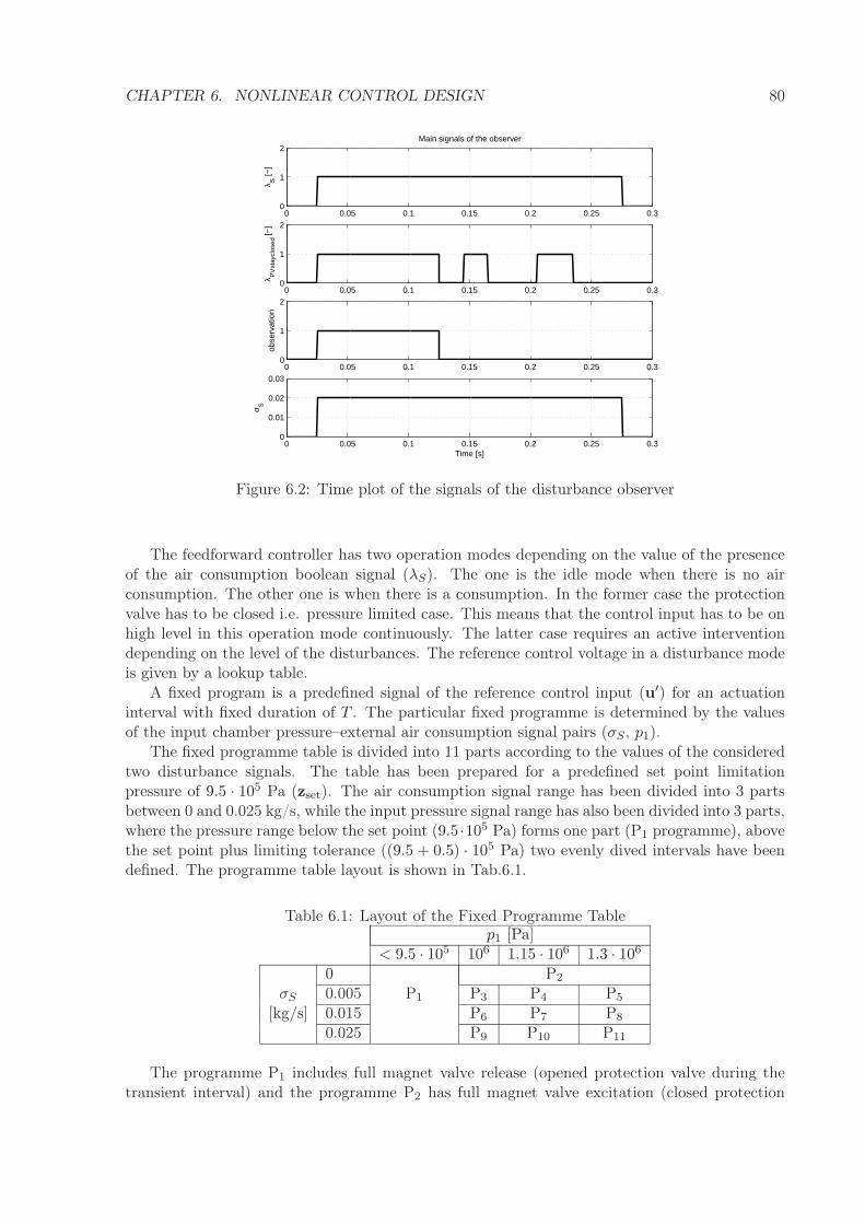
Based on the control aims and the input signal constraints a bang–bang controller has beendeveloped. Since some key disturbance signals are not measurable, a disturbance observer hasbeen added to the controller. The bang–bang controller includes a feedforward– and a feedbackmodule. For verification of the pressure limiting control computer simulations have been utilized.

i

Auszug

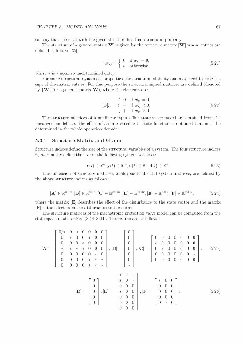
Diese Dissertation befaßt sich mit mechatronischen Überströmventielen verwendet in den Luft-aufbereitungssystemen von Nutzfahrzeugen der neuesten Generation. Das Hauptziel der Arbeitwar die Untersuchung des dynamischen Modells, die Identifikation der unbekannten Modellpa-rameter, die dynamische Analysis des Modells und ein Regelungsdesign für Druckbegrenzung.

Es wurde gezeigt, daß das dynamische Modell des mechatronischen Überströmventiels eineMixtur vom thermodynamischen, mechanischen und elektrodynamischen System ist, wobei diedynamische Gleichungen eine spezielle Struktur haben. Das Modell weist den so genneten hybridAufbau auf.

Das auf physikalische Basis aufgebaute Modell wurde zum Regelungsdesign weitervereinfacht.Zu diesem Zweck wurde ein Vereinfachungskonzept aufgebaut. Die Dimension des Statusvektorswurde reduziert. Der Komplexitätsgrad der algebrischen Strukturen der Modellgleichungen wur-de vereinfacht. Es wurde gezeigt, daß die Struktur der Ein- und Ausgangsvektoren und diephysikalische Bedeutung der Statusvariablen nicht geändert wurde.

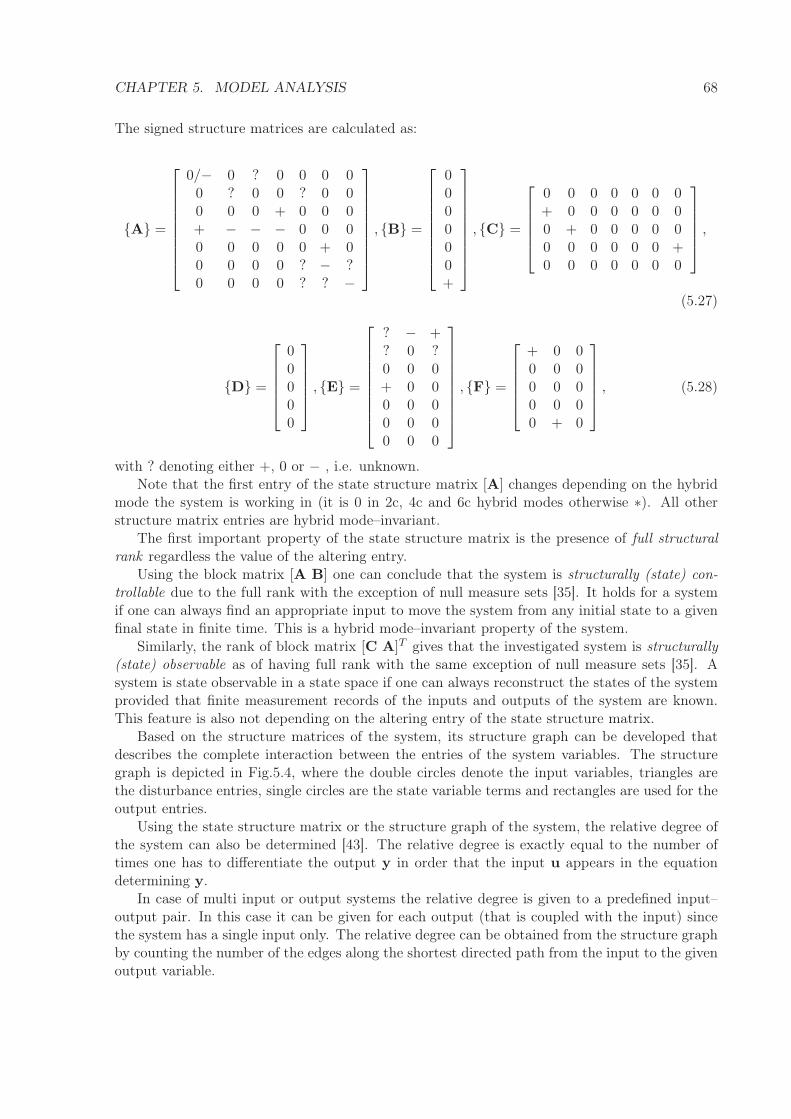
Die unbekannten Modellparameter wurden mit Hilfe von Messungen der dynamischen Ant-wort des realen Systems identifiziert. Das vereinfachte Modell beinhaltet die unbekannte Parame-ter in nichtlinearer Form. Diese Parameter wurden durch die Lösung des generellen Modellparam-terschätzungsproblems mit Beutzung der L2 Norm und der simplexen Optimierung geschätzt.Das kalibrierte Modell wurde durch unabhängige Messungen validiert. Es wurde dargestellt, daßdas validierte Modell das dynamische Benehmen des realen Systems innerhalb der angengebenenToleranz beschreiben kann.

Die Ananlysis des Modells hat gezeigt, daß das Modell auf standardisiertes eingangsaffinesFormat umgeschrieben werden kann. Weiterhin, es hat einen konstanten Freiheitsgrad unabhän-gig von den Hibridmodi. Das Analysis der Hybridmodi hat es gezeigt, daß jeder im Arbeitsbereichder Regelung befindliche Hibridmodus per Systemeingang erreichbar ist. Die weitere Untersu-chungen zeigten, daß das Modell strukturell statuskontrollierbar, statusbeobachbar und strö-rungsbeobachbar ist, und es hat einen maximalen relativen Grad. Die Stabilitätsuntersuchungenwiesen einen lokalen stabilen Betrieb in den typischen Arbeitspunkten des Druckbegrenzungs-reglers auf.

Entsprechend den Regelungszielen und den Begrenzungen am Systemeingang wurde ein bang-bang Regler verwendet. Da gewiße Störungssignale nicht meßbar sind, die Regelung wurde miteinem Strörungssignalbeobachter erweitert. Der bang-bang Regler besteht aus einem feedforwardund einem feedback Teil. Die Verifikation der Regelung wurde durch Simulationen bewertet.

ii

Tartalmi kivonat

A disszertáció mechatronikus védőszelepekkel foglalkozik, amelyek haszonjárművek légfékrend-szereiben alkalmazott új generációs levegőelőkészítő moduljaiban találhatók meg. A vizsgálattárgya a mechatronikus védőszelep dinamikus modellezése, a modell szabályozó–tervezés céljáravaló egyszerűsítése, az ismeretlen modell paraméterek becslése, valamint a modell dinamikusanalízise és egy nyomáskorlátozó szabályozó tervezése.

A vizsgálat megmutatta, hogy a mechatronikus védőszelep egy vegyes termodinamikai, me-chanikai és elektro–dinamikai rendszer, amelynek modellje szisztematikus modellezési eljárássalfelépíthető és verifikálható. Az így felépített nemlineáris dinamikus modell speciális struktúrájú.A modell hibrid, másnéven diszkrét–folytonos elemeket is tartalmaz.

A fizikai törvényszerűségek felhasználásával megalkotott modellt a szerző szabályozó–tervezéscéljára tovább egyszerűsítette. E célból egy modellegyszerűsítési eljárást dolgozott ki. A modellegyszerűsítése révén csökkent az állapot vektor dimenziója és jelentősen egyszerűsödött az egyen-letek algebrai alakja. A vizsgálat kimutatta, hogy a bemeneti–kimeneti vektorok nem változtakaz egyszerűsítés során, valamint, hogy a rendszer változói megtartják fizikai jelentésüket.

A modell ismeretlen paramétereit a valós rendszer dinamikus válaszai segítségével határoztameg a szerző. Az egyszerűsített modell az ismeretlen paramétereket nemlineáris formában tar-talmazza. Az ismeretlen paraméterek az általános paraméter becslési eljárás L2 normán alapulódirekt kereséses optimalizációs módszerével kerültek megállapításra. A kalibrált modell validá-lása független mérések segítségével történt. A vizsgálat bebizonyította, hogy a modell alkalmasa valós rendszer dinamikus viselkedésének megadott tolerancia szinten belüli leírására.

A modellanalízis során a szerző megmutatta, hogy a modell standard input affin alakra hoz-ható, valamint, hogy a modell szabadságfoka a hibrid állapotoktól függetlenül konstans. A hibridviselkedés elérhetőségi vizsgálataival megállapította, hogy a nyomáskorlátozó szabályozó műkö-dési tartományán belüli hibrid állapotok mind elérhetők a modell bemeneti változója segítségével.Ezenkívül a szerző azt is igazolta, hogy az egyszerűsített modell strukturálisan állapot– és zava-rás megfigyelhető, állapot–irányítható és maximális relatív fokkal rendelkezik. A nyitott rendszerstabilitási vizsgálata megmutatta, hogy a nyomáskorlátozó a két jellemző munkapont típusábana rendszer lokálisan stabil.

A szabályozási célok és a bemeneti jelre előírt korlátozás alapján egy bang–bang szabályozókerült kifejlesztésre. Mivel a rendszer nem mindegyik zavarása mérhető, ezért a szabályozásegy zavarás megfigyelővel egészült ki. A bang–bang szabályozó egy zavarás előrecsatolással ésegy modell prediktív visszacsatolásos szabályozóval került kialakításra. A tervezett szabályozótulajdonságait a szerző szimulációk segítségével ellenőrizte.

iii

Foreword

This thesis summarizes the contributions of my research work for obtaining Ph.D. degree inScience of Vehicles and Mobile Machines at the Faculty of Transportation Engineering of theBudapest University of Technology and Economics. The scientific part of the studies has beenmostly undertaken at the Knorr-Bremse Research and Development Centre Budapest and theSystems and Control Laboratory, Computer and Automation Research Institute of the HungarianAcademy of Sciences.

This work would have never been written without the help, continuous support and encou-ragement of several people. First of all, I want to express my sincere gratitude to my supervisorand head of the Knorr-Bremse R&D Center Budapest, Professor László Palkovics, for his patientguidance throughout my studies and support for realizing the opportunities for the experiments.

I express my thank to the fellowship of the Department of Automobiles at the BudapestUniversity of Technology and Economics for the helpful and supporting environment.

I gratefully thank to Professor Katalin M. Hangos, the head of the Process Control ResearchGroup in the Systems and Control Laboratory, Computer and Automation Research Instituteof the Hungarian Academy of Sciences, coauthor of many publications of mine for her excellentand tireless support and many reviews that inspired me to improve my papers significantly.

I would like to express my gratitude to Professor József Bokor, the head of Systems andControl Laboratory for providing me with the essential ideas and literature on nonlinear controlsystems. I am also grateful to my fellow students, Piroska Ailer, Zoltán Bordács and GáborSzederkényi for the joint work.

Finally, I am grateful to my wife Csilla and my parents for supporting my studies in manyways for such a long time.

The undersigned, Huba Németh declares that this Ph.D. thesis has been prepared by himselfas well as that the indicated sources have been used only. All parts that have been taken overliterally or by content are cited unambiguously.

Alulírott Németh Huba kijelentem, hogy ezt a doktori értekezést magam készítettem és abbancsak a megadott forrásokat használtam fel. Minden olyan részt, amelyet szó szerint, vagy azo-nos tartalomban, de átfogalmazva más forrásból átvettem, egyértelműen, a forrás megadásávalmegjelöltem.

Budapest, 2004.06.30.

. . . . . . . . . . . . . . . . . . . . . . . . . . .

iv

Contents

Abstract i

Auszug ii

Tartalmi kivonat iii

Foreword iv

Contents v

List of Figures ix

List of Tables xi

1 Introduction 11.1 Problem Setup and Motivation . . . . . . . . . . . . . . . . . . . . . . . . . . . . 11.2 Literature Review . . . . . . . . . . . . . . . . . . . . . . . . . . . . . . . . . . . . 3

1.2.1 Development of Pneumatic Brake Control of Commercial Vehicles . . . . . 31.2.2 Modelling and Control of Brake Systems Using Modern Approaches . . . 51.2.3 Modelling and Control of Pneumatic Systems . . . . . . . . . . . . . . . . 51.2.4 Results in Nonlinear System and Control Theory Related to this Thesis . 6

1.3 Target Setup . . . . . . . . . . . . . . . . . . . . . . . . . . . . . . . . . . . . . . 61.4 Layout of the Thesis . . . . . . . . . . . . . . . . . . . . . . . . . . . . . . . . . . 71.5 Nomenclature . . . . . . . . . . . . . . . . . . . . . . . . . . . . . . . . . . . . . . 9

2 Nonlinear Hybrid Model 112.1 System Definition . . . . . . . . . . . . . . . . . . . . . . . . . . . . . . . . . . . . 122.2 Modelling Goals . . . . . . . . . . . . . . . . . . . . . . . . . . . . . . . . . . . . . 142.3 Assumptions . . . . . . . . . . . . . . . . . . . . . . . . . . . . . . . . . . . . . . 152.4 Nominal Hybrid Mode . . . . . . . . . . . . . . . . . . . . . . . . . . . . . . . . . 152.5 Conservation Equations . . . . . . . . . . . . . . . . . . . . . . . . . . . . . . . . 16

2.5.1 Conservation of Gas Mass . . . . . . . . . . . . . . . . . . . . . . . . . . . 162.5.2 Conservation of Gas Energy . . . . . . . . . . . . . . . . . . . . . . . . . . 172.5.3 Conservation of Protection Valve Piston Momentum . . . . . . . . . . . . 182.5.4 Conservation of Magnet Valve Armature Momentum . . . . . . . . . . . . 192.5.5 Conservation of Magnetic Linkage . . . . . . . . . . . . . . . . . . . . . . 20

2.6 Constitutive Equations . . . . . . . . . . . . . . . . . . . . . . . . . . . . . . . . . 212.6.1 Chamber Gas Properties . . . . . . . . . . . . . . . . . . . . . . . . . . . . 212.6.2 Forces Acting on the Protection Valve Piston . . . . . . . . . . . . . . . . 222.6.3 Airflow Properties of the Protection Valve . . . . . . . . . . . . . . . . . . 22

v

CONTENTS vi

2.6.4 Forces Acting on the Magnet Valve Armature . . . . . . . . . . . . . . . . 232.6.5 Airflow Properties of the Magnet Valve . . . . . . . . . . . . . . . . . . . 242.6.6 Electro–Magnetic Relations . . . . . . . . . . . . . . . . . . . . . . . . . . 24

2.7 Hybrid Items . . . . . . . . . . . . . . . . . . . . . . . . . . . . . . . . . . . . . . 252.7.1 Gas Enthalpy . . . . . . . . . . . . . . . . . . . . . . . . . . . . . . . . . . 252.7.2 Cross-sections and Stroke Limiting . . . . . . . . . . . . . . . . . . . . . . 262.7.3 Air flows . . . . . . . . . . . . . . . . . . . . . . . . . . . . . . . . . . . . . 26

2.8 Model Equations in State Space Form . . . . . . . . . . . . . . . . . . . . . . . . 272.8.1 State Equation . . . . . . . . . . . . . . . . . . . . . . . . . . . . . . . . . 282.8.2 Output Equation . . . . . . . . . . . . . . . . . . . . . . . . . . . . . . . . 30

2.9 Model Verification . . . . . . . . . . . . . . . . . . . . . . . . . . . . . . . . . . . 302.9.1 System fill up process . . . . . . . . . . . . . . . . . . . . . . . . . . . . . 312.9.2 Circuit defect situation . . . . . . . . . . . . . . . . . . . . . . . . . . . . . 312.9.3 Circuit pressure limiting . . . . . . . . . . . . . . . . . . . . . . . . . . . . 31

2.10 Summary . . . . . . . . . . . . . . . . . . . . . . . . . . . . . . . . . . . . . . . . 32

3 Model Simplification 333.1 The Model Simplification Approach . . . . . . . . . . . . . . . . . . . . . . . . . . 34

3.1.1 The Structure of the Model Elements . . . . . . . . . . . . . . . . . . . . . 343.1.2 Sensitivity analysis . . . . . . . . . . . . . . . . . . . . . . . . . . . . . . . 343.1.3 Methodology . . . . . . . . . . . . . . . . . . . . . . . . . . . . . . . . . . 353.1.4 General Applicability . . . . . . . . . . . . . . . . . . . . . . . . . . . . . . 35

3.2 Test Cases and Decision Making . . . . . . . . . . . . . . . . . . . . . . . . . . . 363.3 Simplification of Balance Volumes . . . . . . . . . . . . . . . . . . . . . . . . . . . 38

3.3.1 Simplification 1: Input Chamber Dynamics Neglected . . . . . . . . . . . 383.3.2 Effect Analysis of Simplification 1 . . . . . . . . . . . . . . . . . . . . . . . 38

3.4 Simplification of Balance Equations . . . . . . . . . . . . . . . . . . . . . . . . . . 383.4.1 Simplification 2: Gas Temperature Dynamics Neglected . . . . . . . . . . 383.4.2 Effect Analysis of Simplification 2 . . . . . . . . . . . . . . . . . . . . . . . 39

3.5 Simplifications of Constitutive Equations . . . . . . . . . . . . . . . . . . . . . . . 403.5.1 Simplification 3: Continuous Streaming Cross Section Equation . . . . . . 403.5.2 Simplification 4: Subsonic Reverse MV Input Air Flow . . . . . . . . . . . 403.5.3 Simplification 5: Sonic MV Exhaust Air Flow . . . . . . . . . . . . . . . . 403.5.4 Effect Analysis of Simplifications 3–5 . . . . . . . . . . . . . . . . . . . . . 41

3.6 Simplified State Space Model . . . . . . . . . . . . . . . . . . . . . . . . . . . . . 413.6.1 State Equation . . . . . . . . . . . . . . . . . . . . . . . . . . . . . . . . . 423.6.2 Output Equation . . . . . . . . . . . . . . . . . . . . . . . . . . . . . . . . 43

3.7 Summary . . . . . . . . . . . . . . . . . . . . . . . . . . . . . . . . . . . . . . . . 43

4 System Identification 454.1 The Investigated Electro–Pneumatic System . . . . . . . . . . . . . . . . . . . . . 464.2 The Measurement System . . . . . . . . . . . . . . . . . . . . . . . . . . . . . . . 474.3 Statistical Signal Quality Evaluation . . . . . . . . . . . . . . . . . . . . . . . . . 48

4.3.1 Descriptive Statistics . . . . . . . . . . . . . . . . . . . . . . . . . . . . . . 484.3.2 Normality Assessment . . . . . . . . . . . . . . . . . . . . . . . . . . . . . 504.3.3 Time Domain Analysis . . . . . . . . . . . . . . . . . . . . . . . . . . . . . 504.3.4 Frequency Domain Analysis . . . . . . . . . . . . . . . . . . . . . . . . . . 50

4.4 Operation Domain . . . . . . . . . . . . . . . . . . . . . . . . . . . . . . . . . . . 514.5 Sensitivity Analysis . . . . . . . . . . . . . . . . . . . . . . . . . . . . . . . . . . . 51

CONTENTS vii

4.5.1 Parameter Clustering . . . . . . . . . . . . . . . . . . . . . . . . . . . . . . 524.5.2 Parametric Sensitivity Assessment . . . . . . . . . . . . . . . . . . . . . . 53

4.6 Dynamic Parameter Estimation . . . . . . . . . . . . . . . . . . . . . . . . . . . . 534.6.1 Parameters to Be Identified . . . . . . . . . . . . . . . . . . . . . . . . . . 534.6.2 The Dynamic Nonlinear Parameter Estimation Method . . . . . . . . . . 554.6.3 Minimizing the Cost Function . . . . . . . . . . . . . . . . . . . . . . . . . 574.6.4 Model Parameter Estimation . . . . . . . . . . . . . . . . . . . . . . . . . 574.6.5 Assessing the Fit . . . . . . . . . . . . . . . . . . . . . . . . . . . . . . . . 58

4.7 Model Validation . . . . . . . . . . . . . . . . . . . . . . . . . . . . . . . . . . . . 594.8 Summary . . . . . . . . . . . . . . . . . . . . . . . . . . . . . . . . . . . . . . . . 59

5 Model Analysis 615.1 Basic Model Properties . . . . . . . . . . . . . . . . . . . . . . . . . . . . . . . . . 62

5.1.1 Nonlinear Input Affine Structure . . . . . . . . . . . . . . . . . . . . . . . 625.1.2 Degrees of Freedom . . . . . . . . . . . . . . . . . . . . . . . . . . . . . . . 62

5.2 Hybrid Analysis . . . . . . . . . . . . . . . . . . . . . . . . . . . . . . . . . . . . . 625.2.1 Hybrid Transitions . . . . . . . . . . . . . . . . . . . . . . . . . . . . . . . 655.2.2 Hybrid Reachability . . . . . . . . . . . . . . . . . . . . . . . . . . . . . . 66

5.3 Structural Dynamic Properties . . . . . . . . . . . . . . . . . . . . . . . . . . . . 665.3.1 Structure Matrix and Graph . . . . . . . . . . . . . . . . . . . . . . . . . . 675.3.2 Disturbance Observability . . . . . . . . . . . . . . . . . . . . . . . . . . . 69

5.4 Disturbance Sensitivity Analysis . . . . . . . . . . . . . . . . . . . . . . . . . . . 705.5 Stability Analysis . . . . . . . . . . . . . . . . . . . . . . . . . . . . . . . . . . . . 71

5.5.1 BIBO Stability . . . . . . . . . . . . . . . . . . . . . . . . . . . . . . . . . 715.5.2 Asymptotic Stability . . . . . . . . . . . . . . . . . . . . . . . . . . . . . . 72

5.6 Summary . . . . . . . . . . . . . . . . . . . . . . . . . . . . . . . . . . . . . . . . 73

6 Nonlinear Control Design 756.1 Control Aims . . . . . . . . . . . . . . . . . . . . . . . . . . . . . . . . . . . . . . 766.2 Control Constraint: Two-level Input . . . . . . . . . . . . . . . . . . . . . . . . . 766.3 Assumptions on the Disturbance . . . . . . . . . . . . . . . . . . . . . . . . . . . 776.4 Controller Structure: Bang-Bang Controller . . . . . . . . . . . . . . . . . . . . . 776.5 Design of the Disturbance Observer . . . . . . . . . . . . . . . . . . . . . . . . . . 786.6 Design of the Feedforward Controller . . . . . . . . . . . . . . . . . . . . . . . . . 79

6.6.1 Optimization Method . . . . . . . . . . . . . . . . . . . . . . . . . . . . . 816.6.2 Optimization Results . . . . . . . . . . . . . . . . . . . . . . . . . . . . . . 82

6.7 Design of the Feedback Controller . . . . . . . . . . . . . . . . . . . . . . . . . . . 846.8 Simulation Results . . . . . . . . . . . . . . . . . . . . . . . . . . . . . . . . . . . 866.9 Discussion . . . . . . . . . . . . . . . . . . . . . . . . . . . . . . . . . . . . . . . . 896.10 Summary . . . . . . . . . . . . . . . . . . . . . . . . . . . . . . . . . . . . . . . . 90

7 Conclusions 917.1 Theses . . . . . . . . . . . . . . . . . . . . . . . . . . . . . . . . . . . . . . . . . . 917.2. Tézisek magyar nyelven . . . . . . . . . . . . . . . . . . . . . . . . . . . . . . . . 937.3 Publications . . . . . . . . . . . . . . . . . . . . . . . . . . . . . . . . . . . . . . . 95

7.3.1 Publications Directly Related to the Thesis . . . . . . . . . . . . . . . . . 957.3.2 Other Publications . . . . . . . . . . . . . . . . . . . . . . . . . . . . . . . 96

7.4 Directions for Future Research . . . . . . . . . . . . . . . . . . . . . . . . . . . . 96

Bibliography 98

CONTENTS viii

A Figures and Tables 106A.1 Model Verification . . . . . . . . . . . . . . . . . . . . . . . . . . . . . . . . . . . 107

A.1.1 Simulation Results . . . . . . . . . . . . . . . . . . . . . . . . . . . . . . . 107A.1.2 Parameter Setup . . . . . . . . . . . . . . . . . . . . . . . . . . . . . . . . 110

A.2 Model Simplification . . . . . . . . . . . . . . . . . . . . . . . . . . . . . . . . . . 111A.2.1 Simulation Results . . . . . . . . . . . . . . . . . . . . . . . . . . . . . . . 111A.2.2 Parameter Setup . . . . . . . . . . . . . . . . . . . . . . . . . . . . . . . . 116

A.3 System Identification and Model Validation . . . . . . . . . . . . . . . . . . . . . 117A.4 Response Functions for the Fixed Programmes . . . . . . . . . . . . . . . . . . . 133

B Program Lists 137B.1 Substitutions of the Detailed Model . . . . . . . . . . . . . . . . . . . . . . . . . . 138B.2 Substitutions of the Simplified Model . . . . . . . . . . . . . . . . . . . . . . . . . 147B.3 Model Linearization . . . . . . . . . . . . . . . . . . . . . . . . . . . . . . . . . . 154

List of Figures

2.1 Layout of the electro–pneumatic brake system of a towing vehicle (4x2) . . . . . 122.2 Internal layout of an electronic air treatment control unit . . . . . . . . . . . . . 132.3 Schematic of the single mechatronic protection valve . . . . . . . . . . . . . . . . 142.4 The protection valve piston with its close surrounding . . . . . . . . . . . . . . . 192.5 Layout of the solenoid magnet valve . . . . . . . . . . . . . . . . . . . . . . . . . 202.6 Electronic circuit diagram of the solenoid magnet valve . . . . . . . . . . . . . . . 202.7 Magnetic circuit diagram of the MV . . . . . . . . . . . . . . . . . . . . . . . . . 23

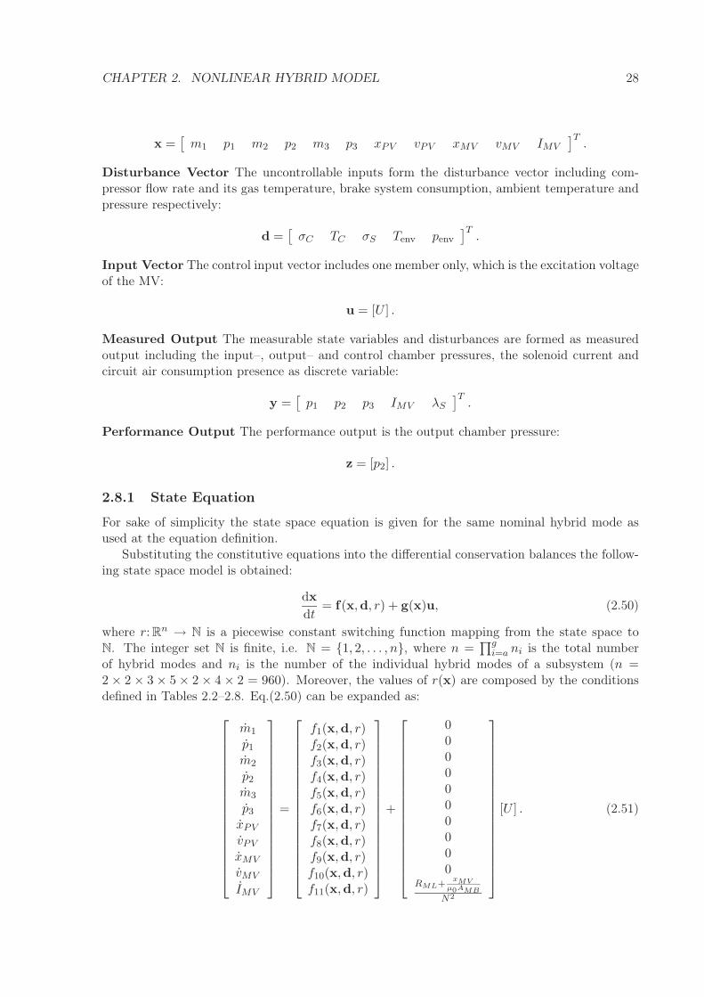
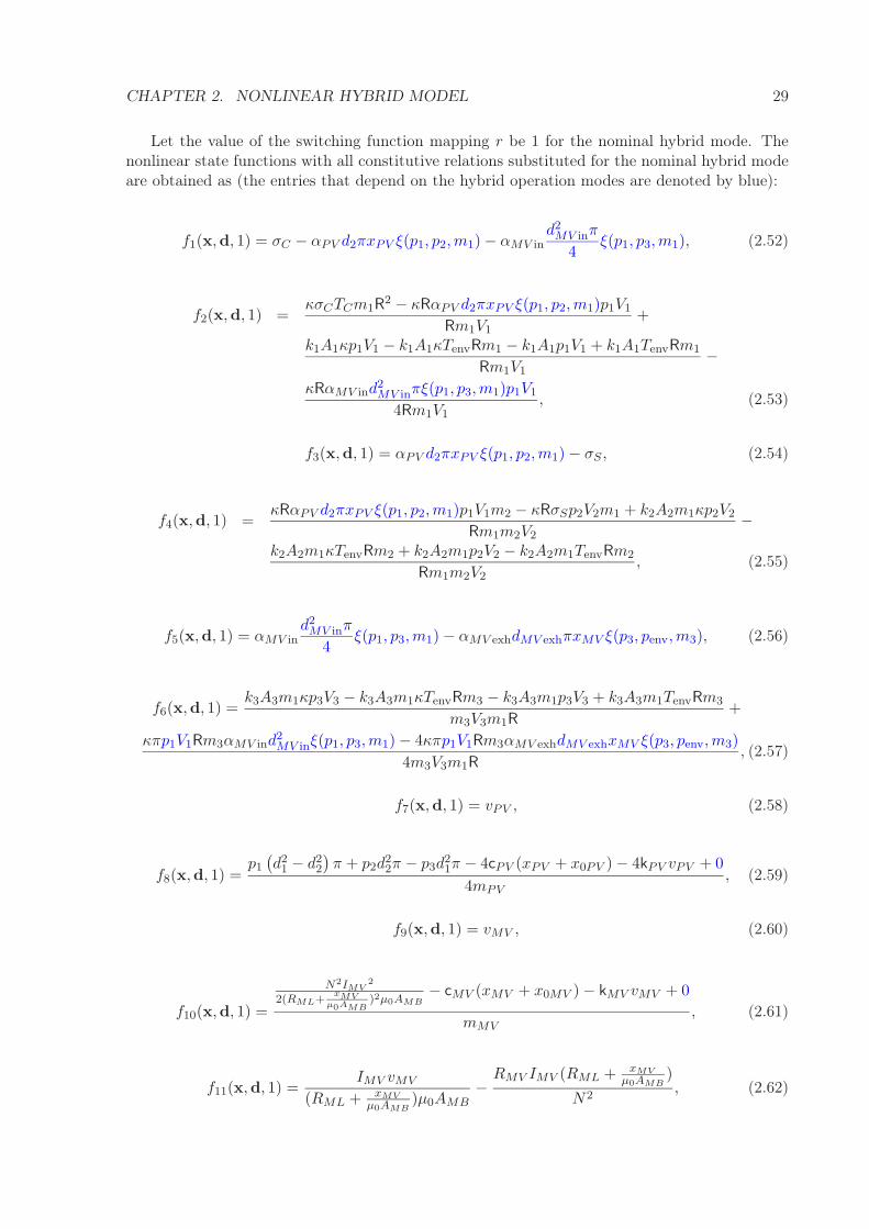
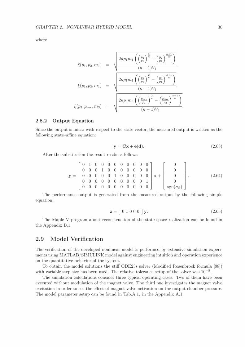
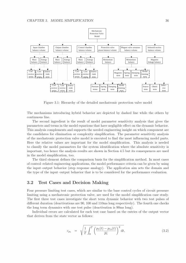
3.1 Hierarchy of the detailed mechatronic protection valve model . . . . . . . . . . . 363.2 Excitation voltage (system input) as function of time in the four test cases . . . . 373.3 Schematic of simplified mechatronic protection valve . . . . . . . . . . . . . . . . 423.4 Hierarchy of the simplified mechatronic protection valve model . . . . . . . . . . 44

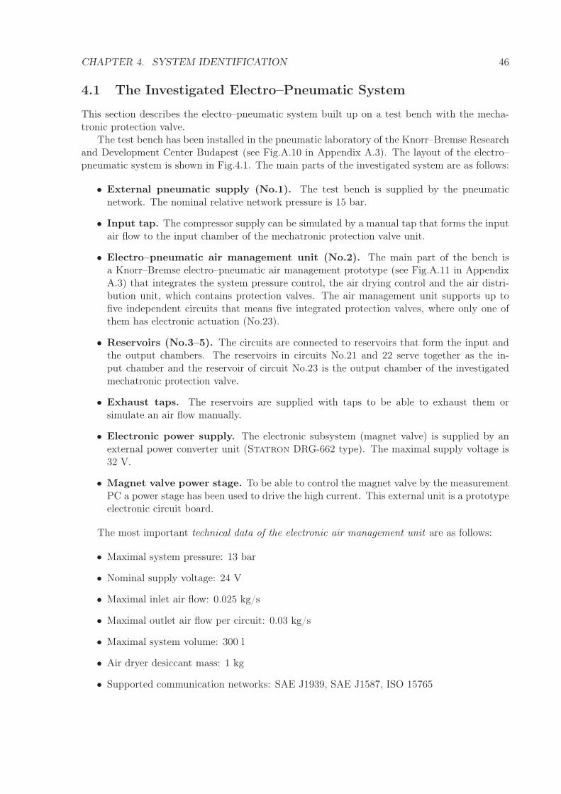
4.1 Schematic of the investigated system on the test bench . . . . . . . . . . . . . . . 47

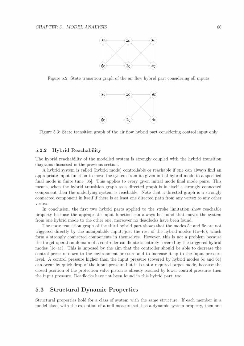
5.1 State transition graphs of the protection- and magnet valve stroke limiting . . . . 655.2 State transition graph of the air flow hybrid part considering all inputs . . . . . . 665.3 State transition graph of the air flow hybrid part considering control input only . 665.4 Structure graph of the model of the mechatronic protection valve . . . . . . . . . 69

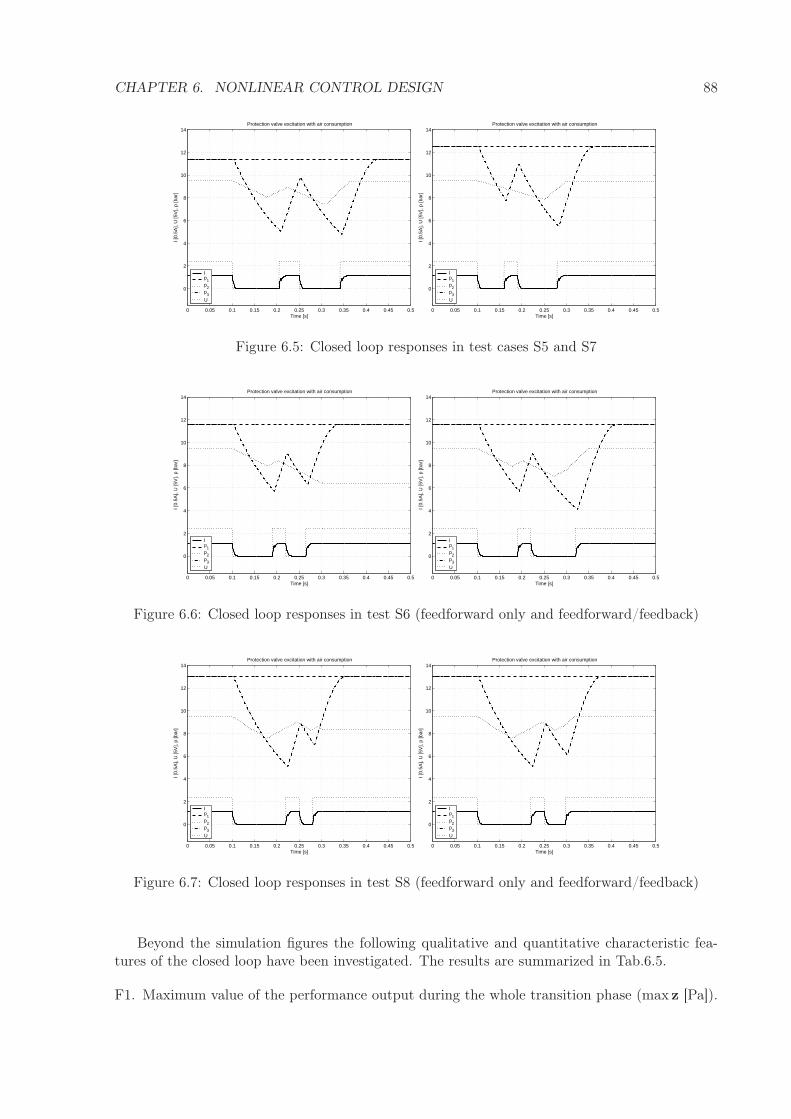
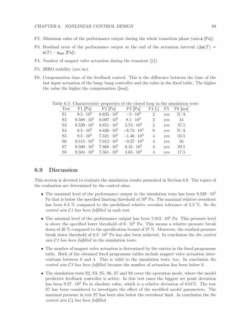
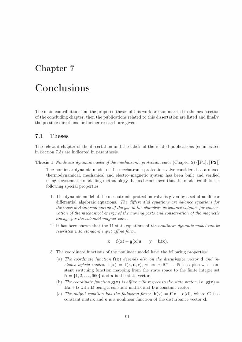
6.1 Block scheme of the closed loop system . . . . . . . . . . . . . . . . . . . . . . . . 786.2 Time plot of the signals of the disturbance observer . . . . . . . . . . . . . . . . . 806.3 Closed loop responses in test cases S1 and S2 . . . . . . . . . . . . . . . . . . . . 876.4 Closed loop responses in test cases S3 and S4 . . . . . . . . . . . . . . . . . . . . 876.5 Closed loop responses in test cases S5 and S7 . . . . . . . . . . . . . . . . . . . . 886.6 Closed loop responses in test S6 (feedforward only and feedforward/feedback) . . 886.7 Closed loop responses in test S8 (feedforward only and feedforward/feedback) . . 88

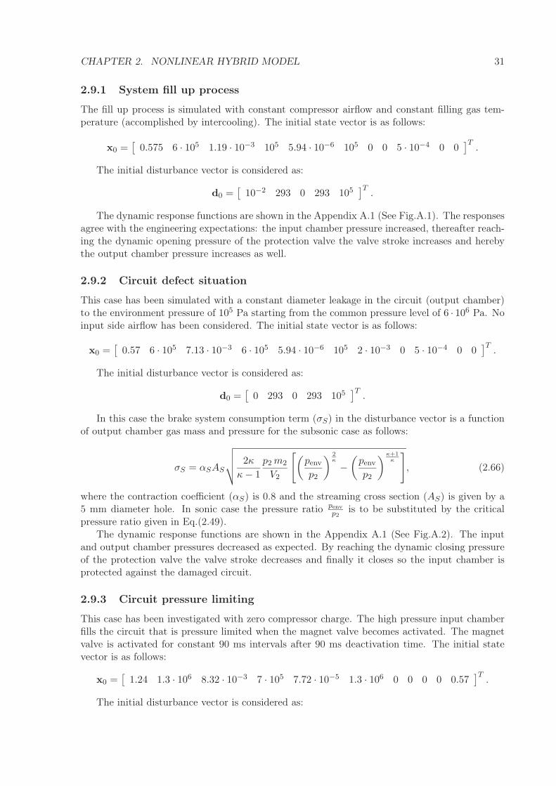
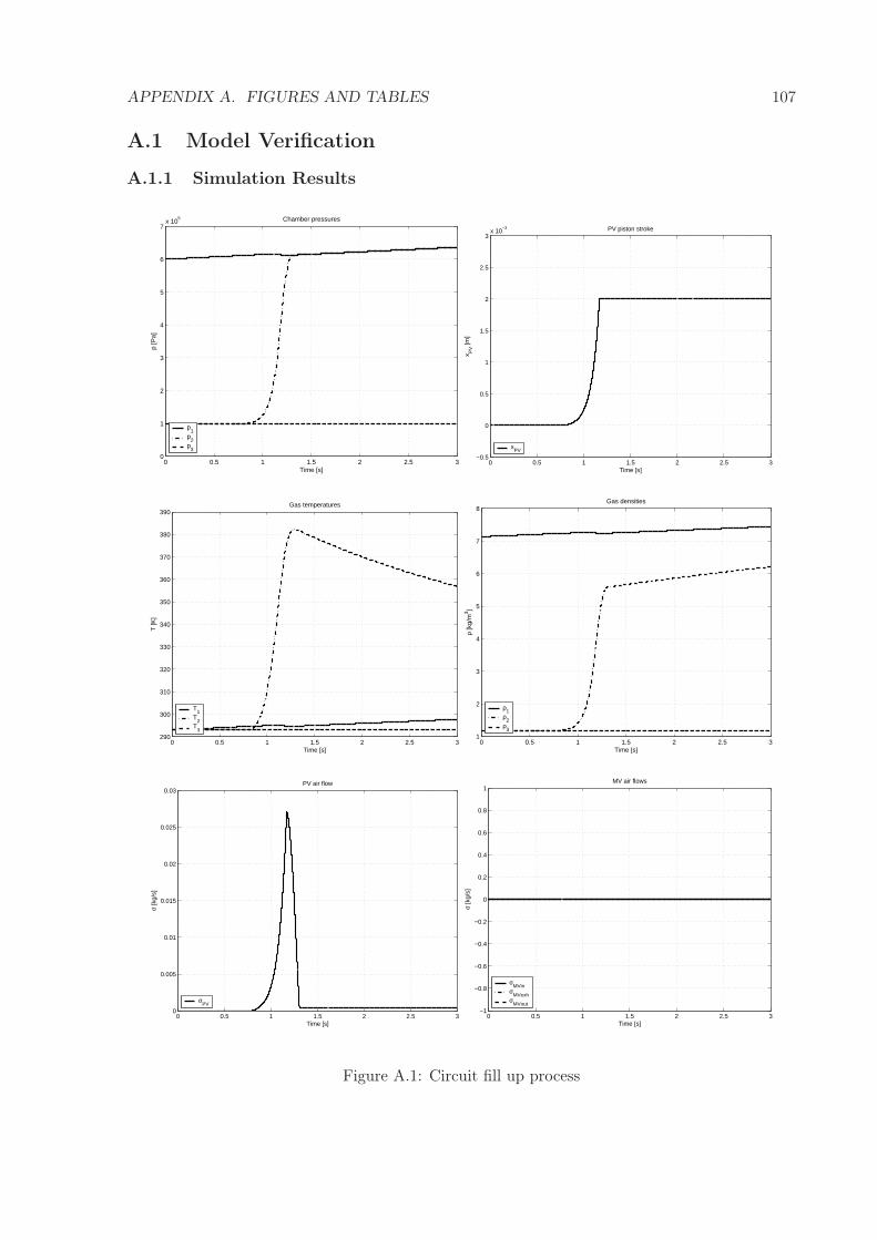
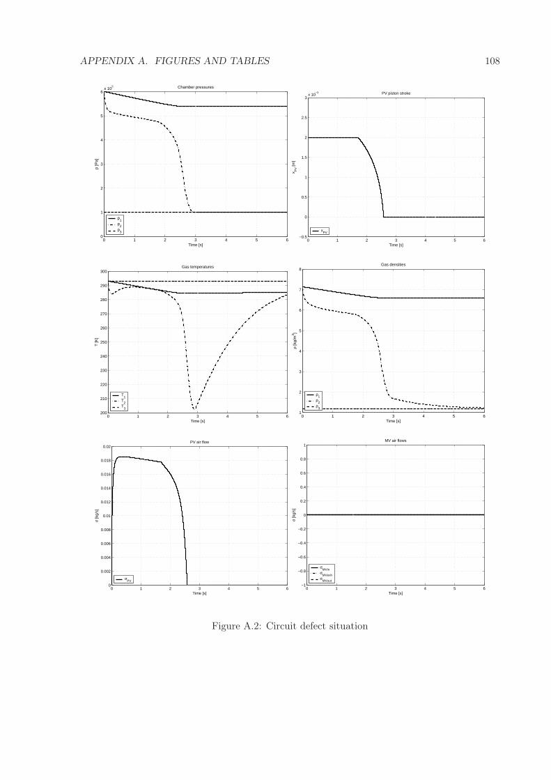
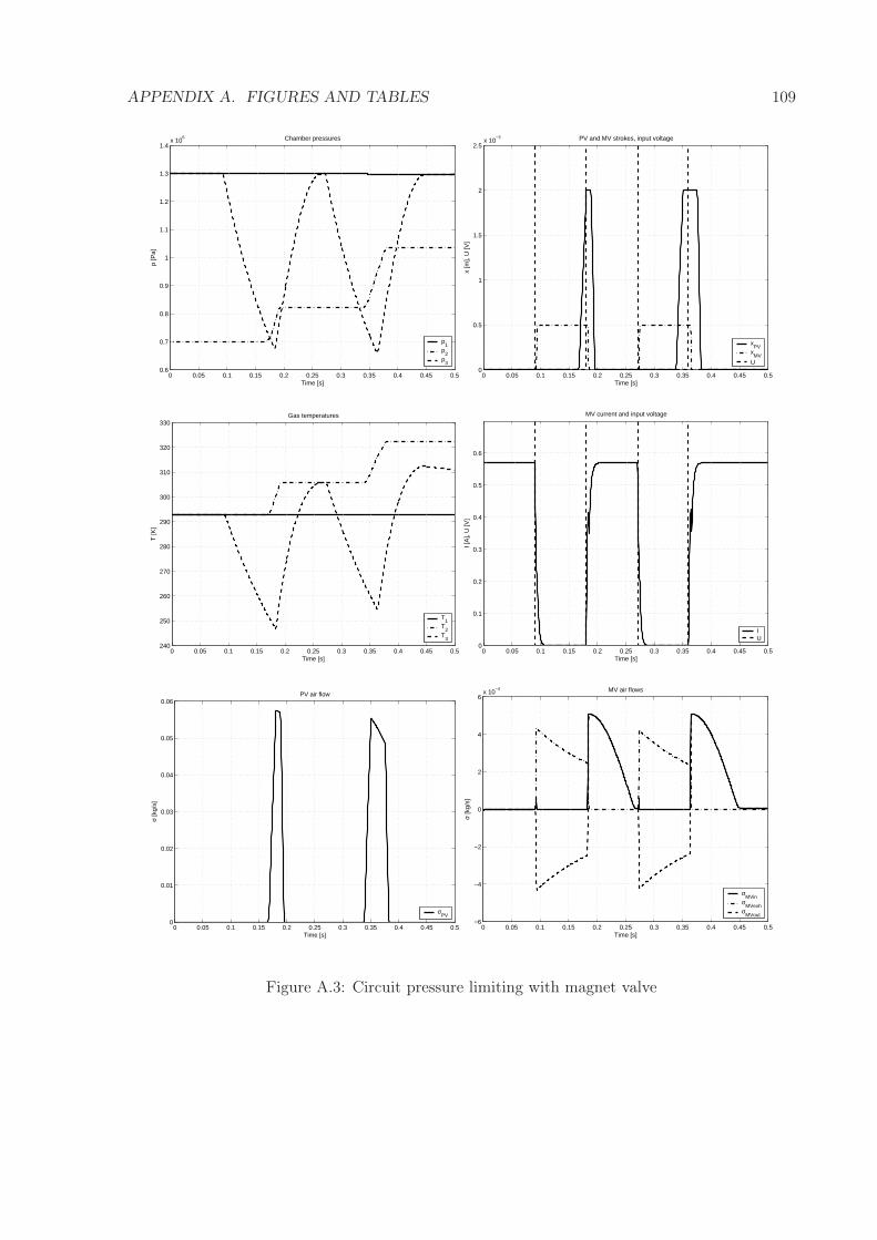
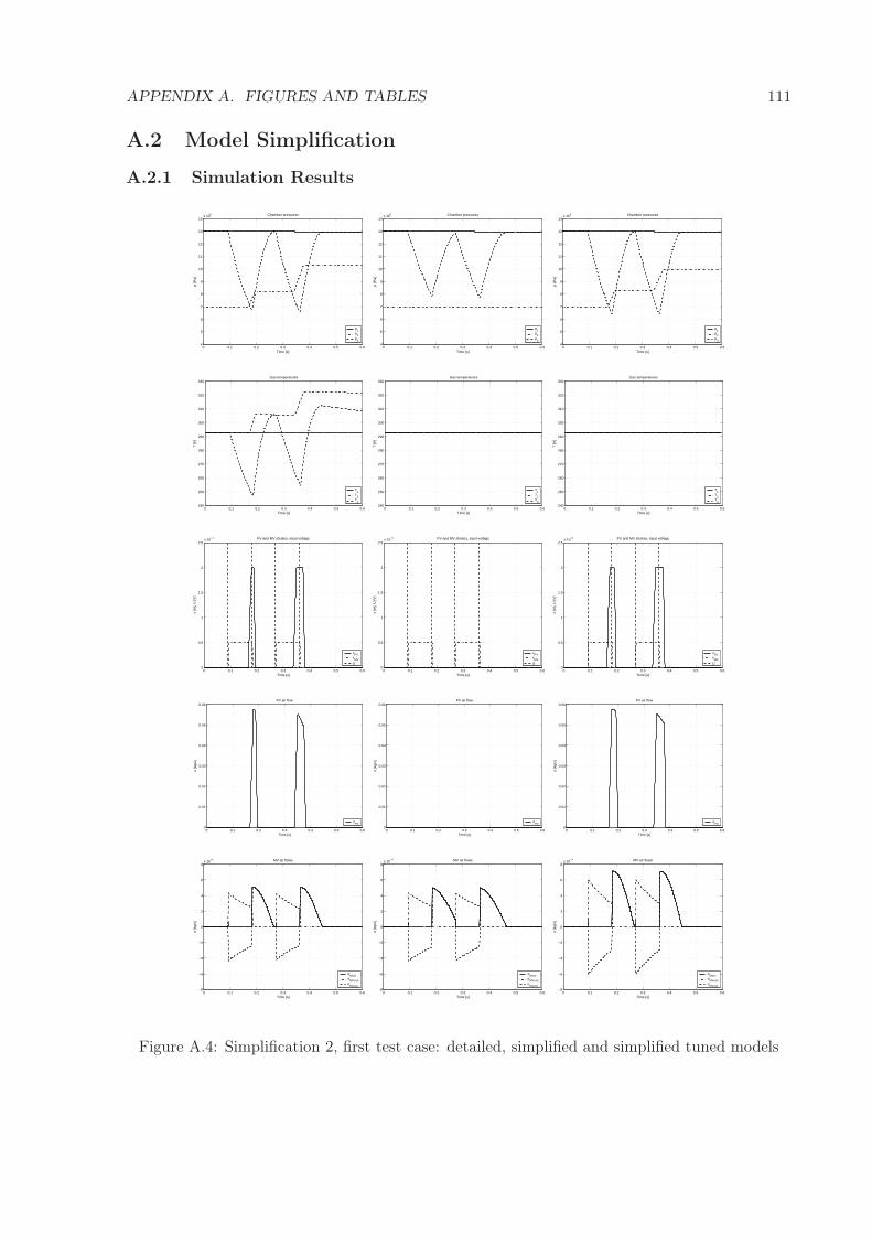
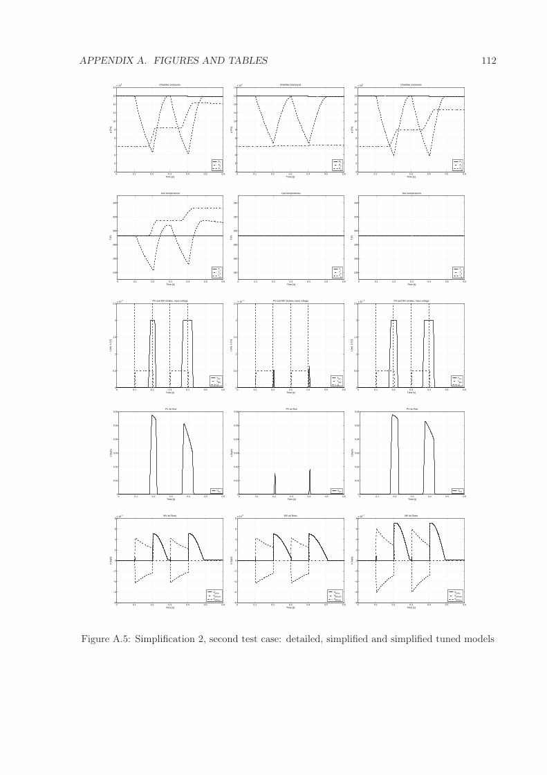
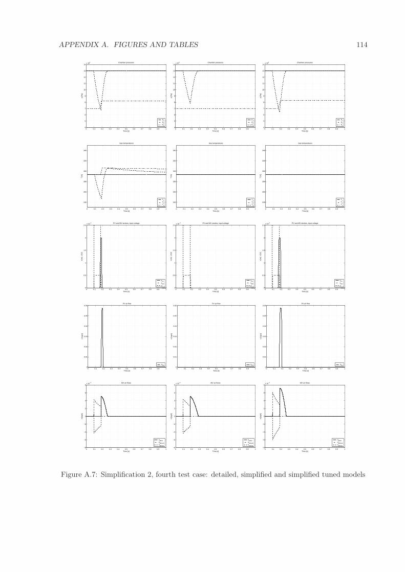
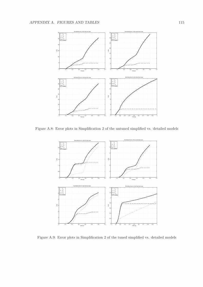
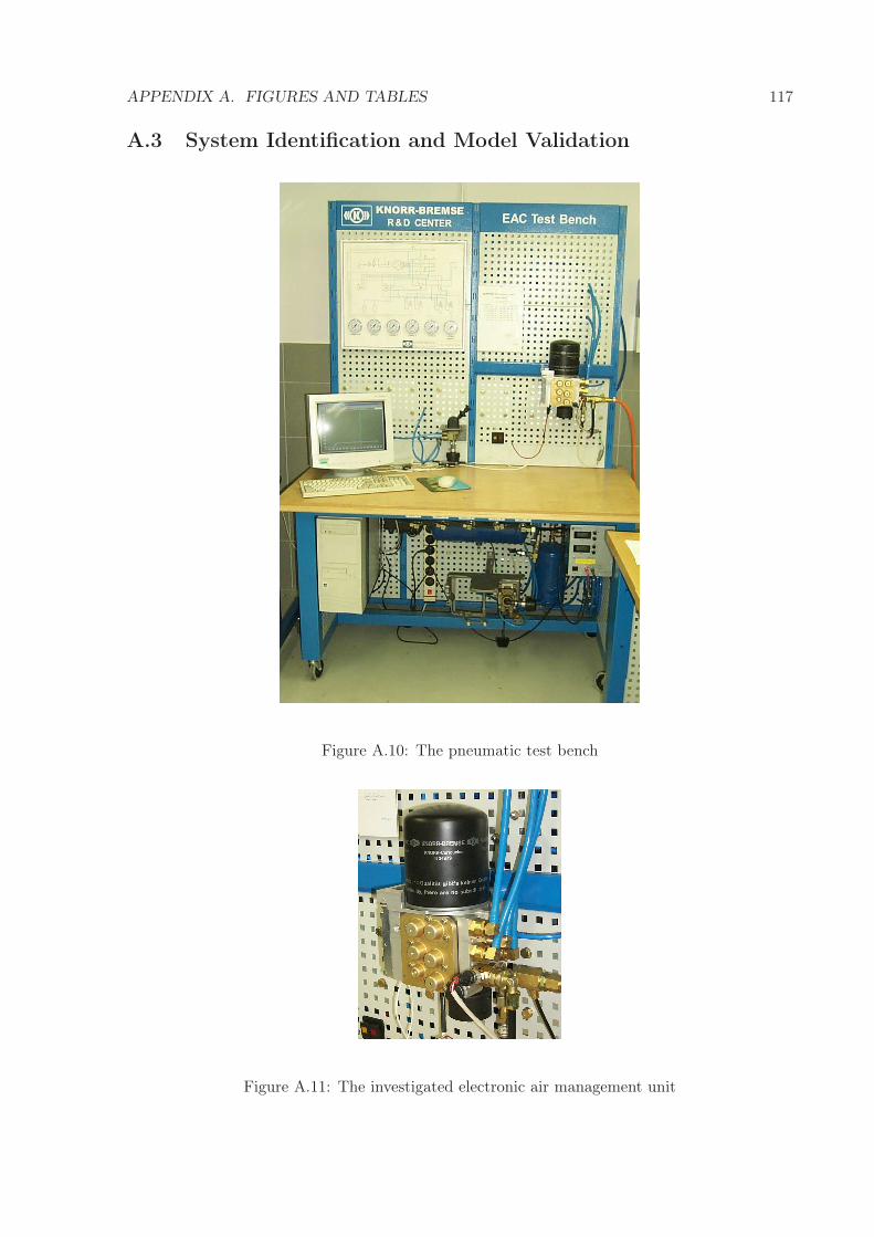
A.1 Circuit fill up process . . . . . . . . . . . . . . . . . . . . . . . . . . . . . . . . . . 107A.2 Circuit defect situation . . . . . . . . . . . . . . . . . . . . . . . . . . . . . . . . . 108A.3 Circuit pressure limiting with magnet valve . . . . . . . . . . . . . . . . . . . . . 109A.4 Simplification 2, first test case: detailed, simplified and simplified tuned models . 111A.5 Simplification 2, second test case: detailed, simplified and simplified tuned models 112A.6 Simplification 2, third test case: detailed, simplified and simplified tuned models 113A.7 Simplification 2, fourth test case: detailed, simplified and simplified tuned models 114A.8 Error plots in Simplification 2 of the untuned simplified vs. detailed models . . . 115A.9 Error plots in Simplification 2 of the tuned simplified vs. detailed models . . . . 115A.10 The pneumatic test bench . . . . . . . . . . . . . . . . . . . . . . . . . . . . . . . 117A.11 The investigated electronic air management unit . . . . . . . . . . . . . . . . . . 117A.12 Acquired data for signal quality check . . . . . . . . . . . . . . . . . . . . . . . . 118

ix

LIST OF FIGURES x

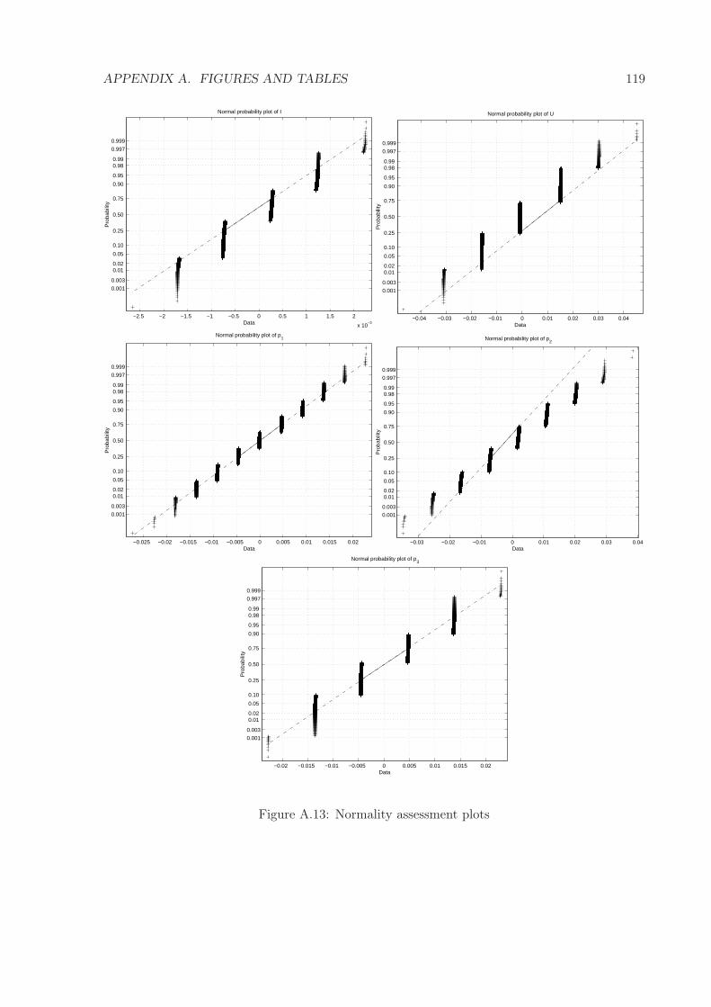
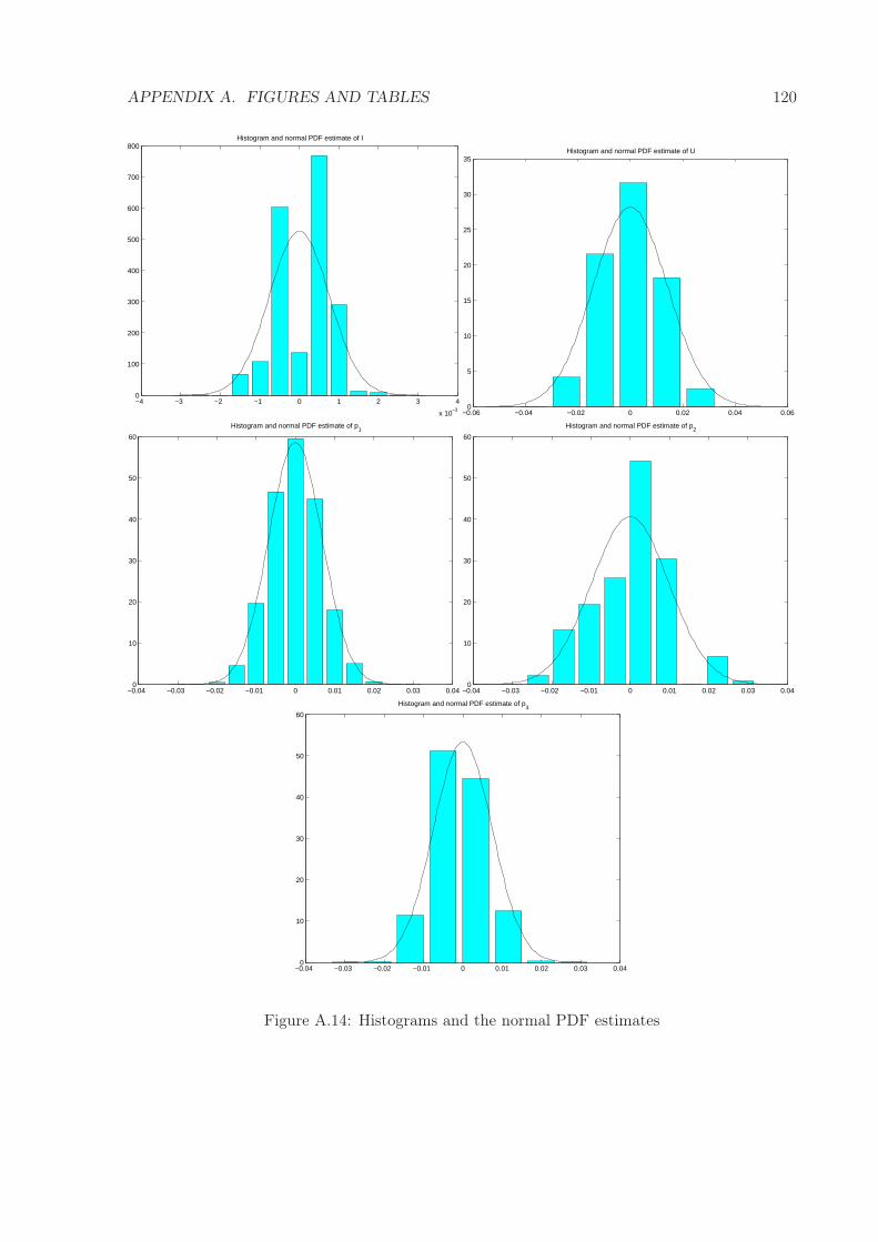
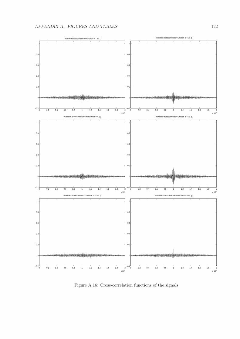
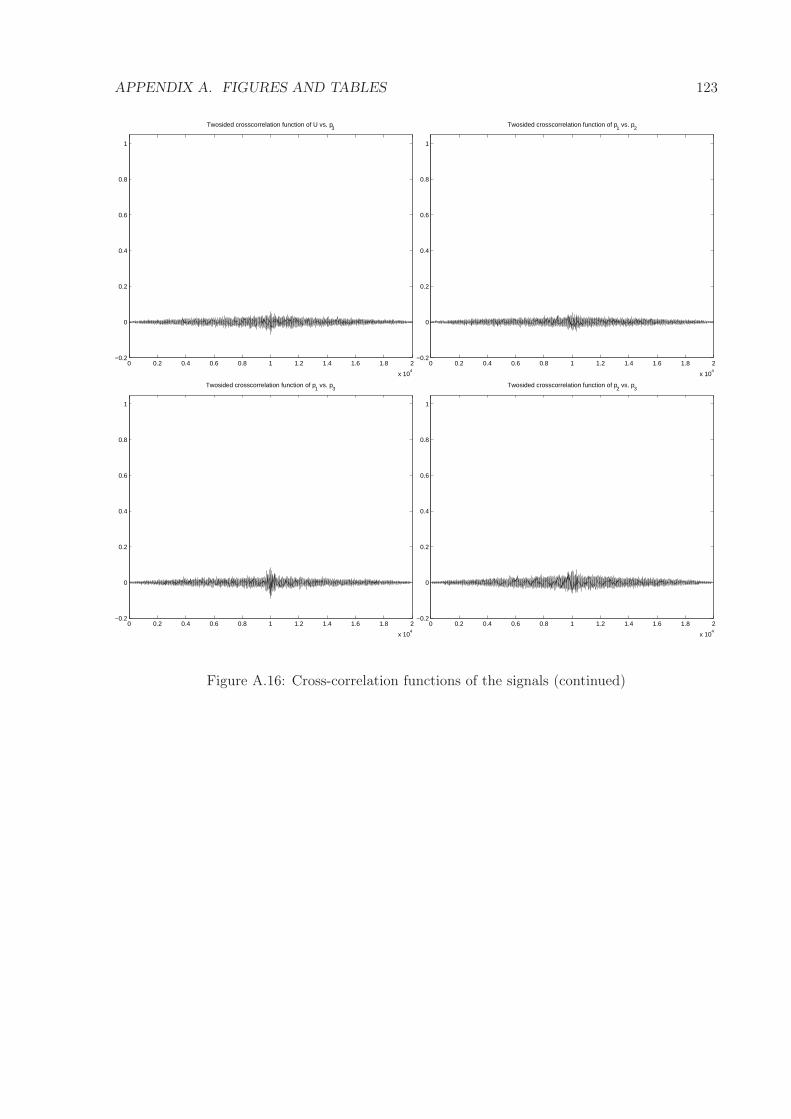
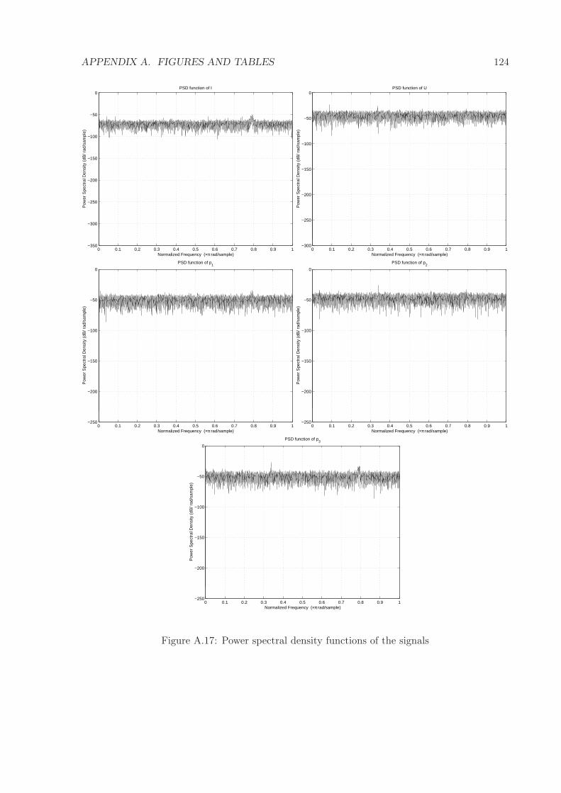
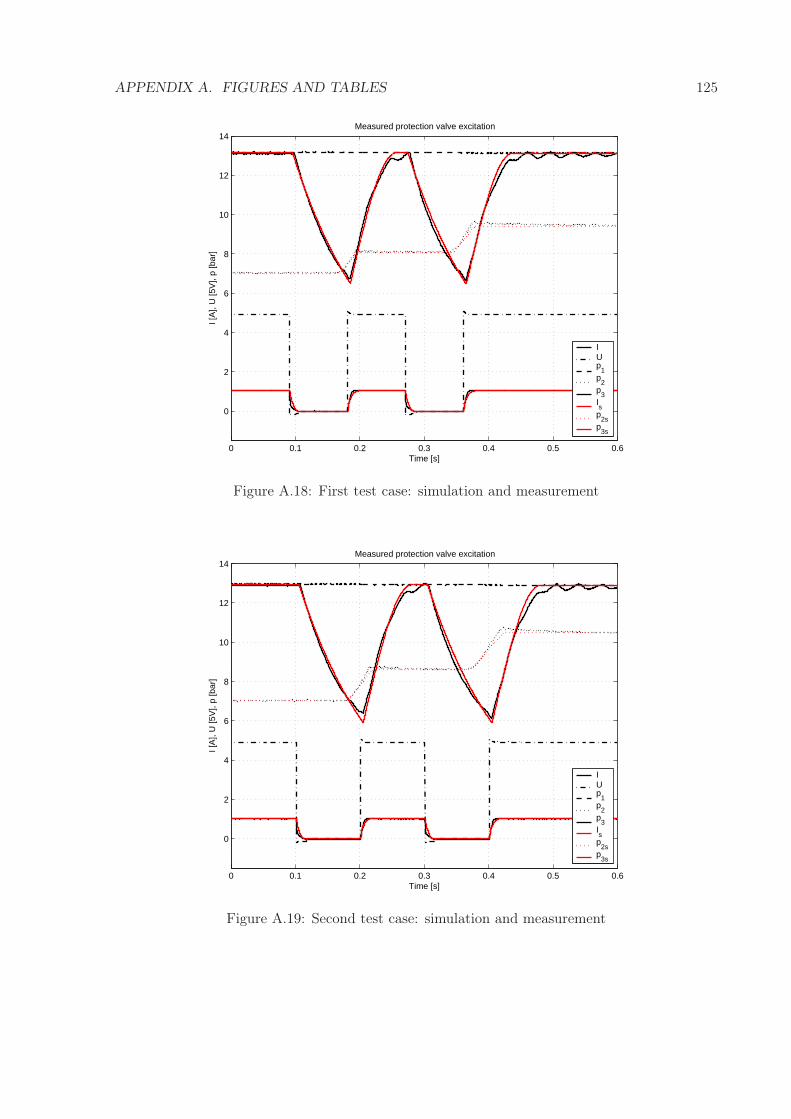
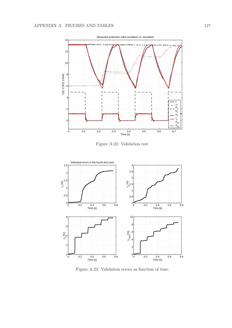
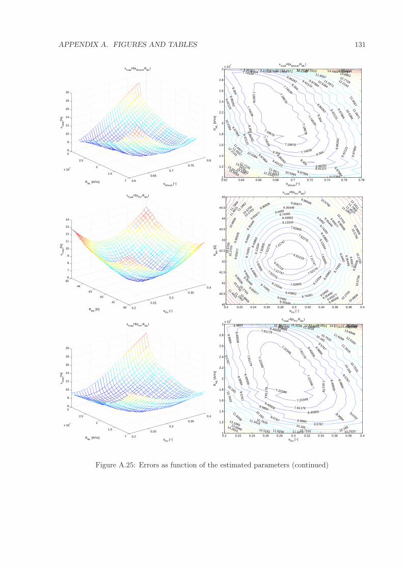
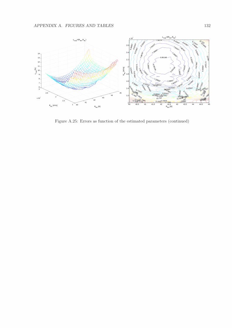
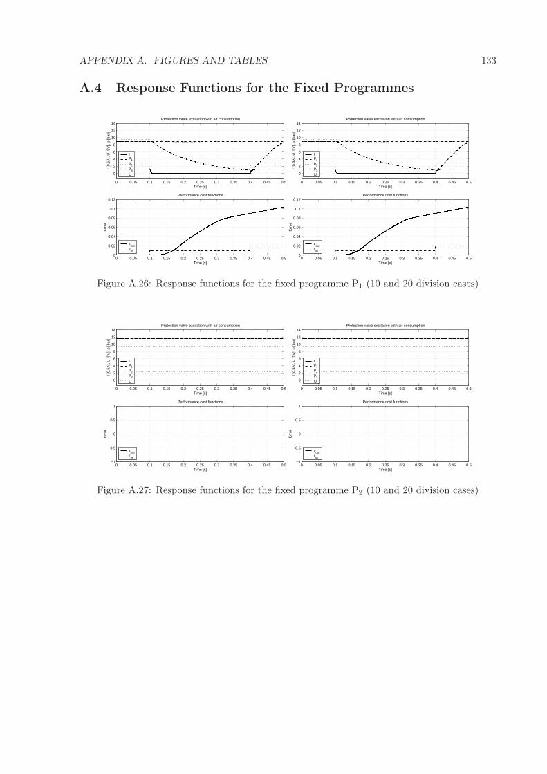
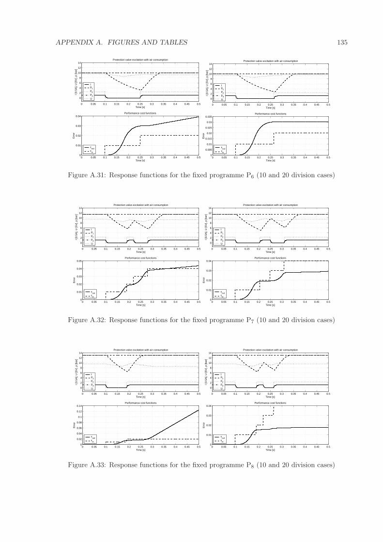
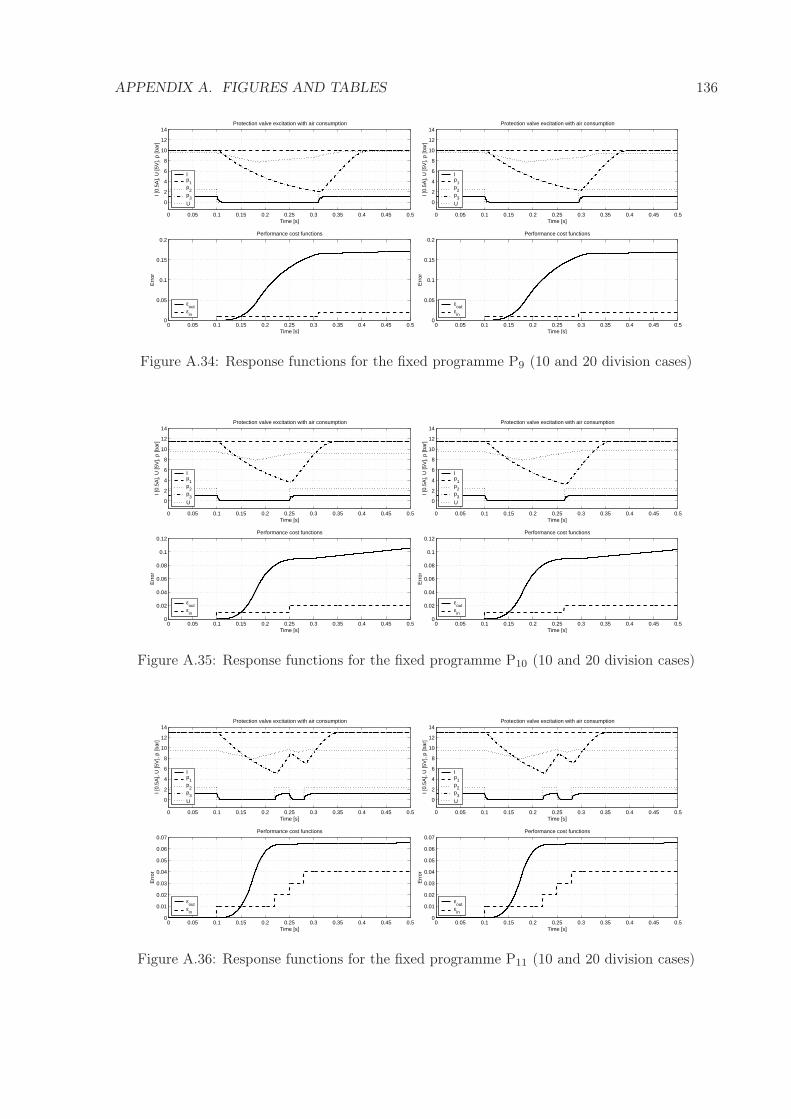
A.13 Normality assessment plots . . . . . . . . . . . . . . . . . . . . . . . . . . . . . . 119A.14 Histograms and the normal PDF estimates . . . . . . . . . . . . . . . . . . . . . . 120A.15 Autocorrelation functions of the signals . . . . . . . . . . . . . . . . . . . . . . . 121A.16 Cross-correlation functions of the signals . . . . . . . . . . . . . . . . . . . . . . . 122A.16 Cross-correlation functions of the signals (continued) . . . . . . . . . . . . . . . . 123A.17 Power spectral density functions of the signals . . . . . . . . . . . . . . . . . . . . 124A.18 First test case: simulation and measurement . . . . . . . . . . . . . . . . . . . . . 125A.19 Second test case: simulation and measurement . . . . . . . . . . . . . . . . . . . 125A.20 Third test case: simulation measurement . . . . . . . . . . . . . . . . . . . . . . . 126A.21 Fourth test case: simulation and measurement . . . . . . . . . . . . . . . . . . . . 126A.22 Validation test . . . . . . . . . . . . . . . . . . . . . . . . . . . . . . . . . . . . . 127A.23 Validation errors as function of time . . . . . . . . . . . . . . . . . . . . . . . . . 127A.24 Errors as function of parameters one by one . . . . . . . . . . . . . . . . . . . . . 128A.25 Errors as function of the estimated parameters . . . . . . . . . . . . . . . . . . . 129A.25 Errors as function of the estimated parameters (continued) . . . . . . . . . . . . . 130A.25 Errors as function of the estimated parameters (continued) . . . . . . . . . . . . . 131A.25 Errors as function of the estimated parameters (continued) . . . . . . . . . . . . . 132A.26 Response functions for the fixed programme P1 (10 and 20 division cases) . . . . 133A.27 Response functions for the fixed programme P2 (10 and 20 division cases) . . . . 133A.28 Response functions for the fixed programme P3 (10 and 20 division cases) . . . . 134A.29 Response functions for the fixed programme P4 (10 and 20 division cases) . . . . 134A.30 Response functions for the fixed programme P5 (10 and 20 division cases) . . . . 134A.31 Response functions for the fixed programme P6 (10 and 20 division cases) . . . . 135A.32 Response functions for the fixed programme P7 (10 and 20 division cases) . . . . 135A.33 Response functions for the fixed programme P8 (10 and 20 division cases) . . . . 135A.34 Response functions for the fixed programme P9 (10 and 20 division cases) . . . . 136A.35 Response functions for the fixed programme P10 (10 and 20 division cases) . . . . 136A.36 Response functions for the fixed programme P11 (10 and 20 division cases) . . . . 136

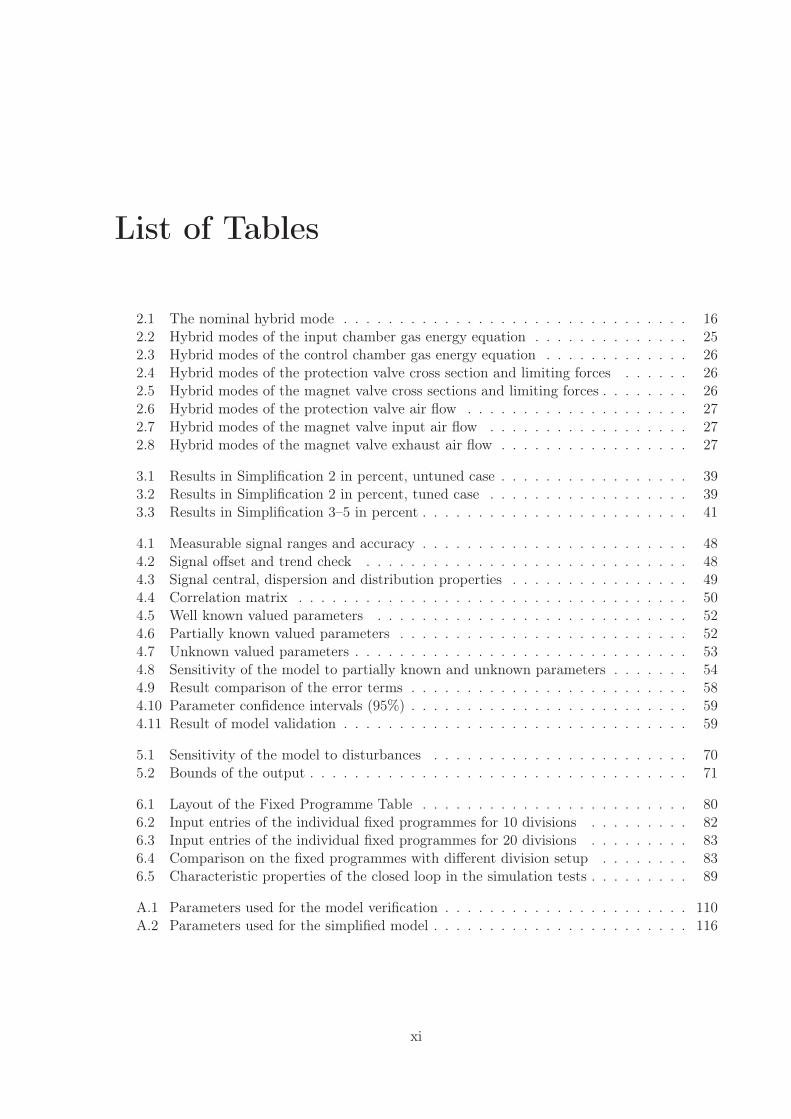
List of Tables

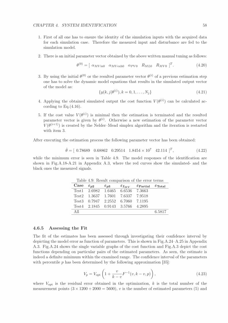
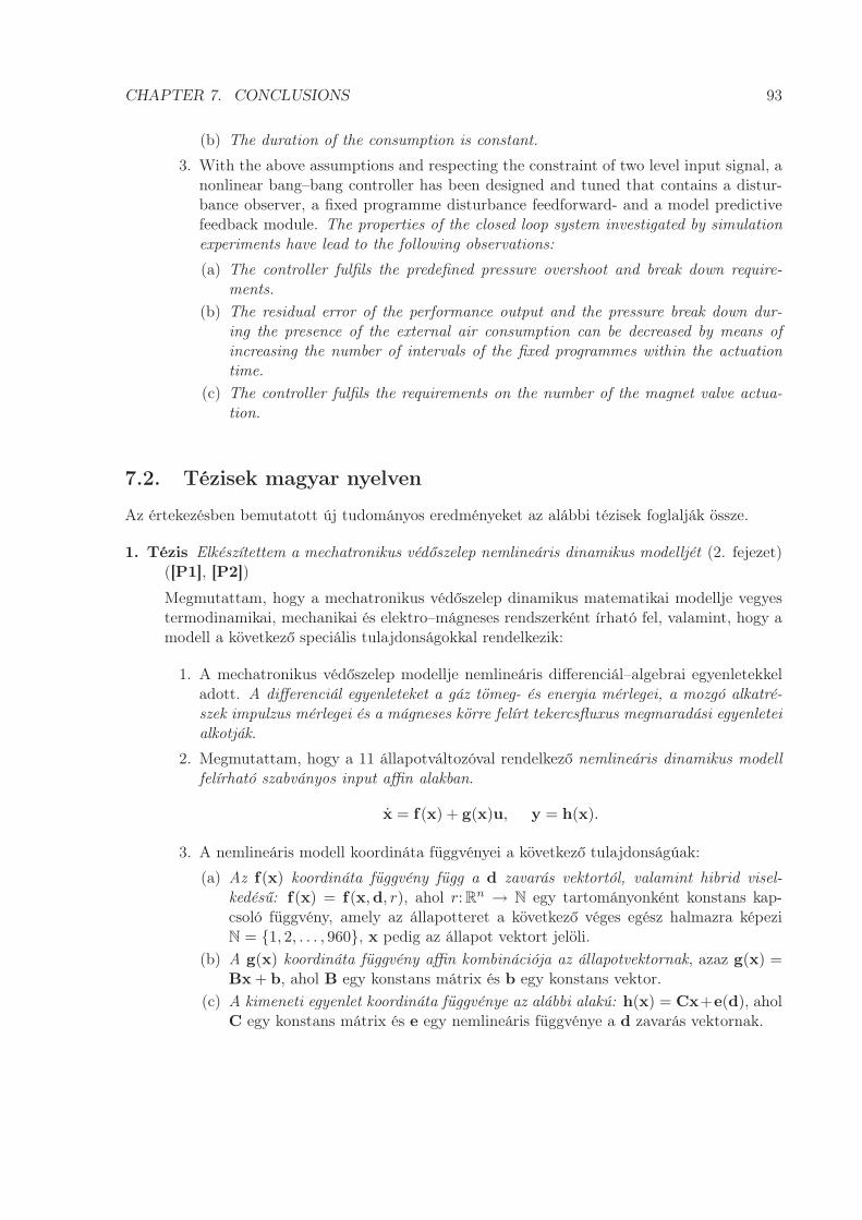
2.1 The nominal hybrid mode . . . . . . . . . . . . . . . . . . . . . . . . . . . . . . . 162.2 Hybrid modes of the input chamber gas energy equation . . . . . . . . . . . . . . 252.3 Hybrid modes of the control chamber gas energy equation . . . . . . . . . . . . . 262.4 Hybrid modes of the protection valve cross section and limiting forces . . . . . . 262.5 Hybrid modes of the magnet valve cross sections and limiting forces . . . . . . . . 262.6 Hybrid modes of the protection valve air flow . . . . . . . . . . . . . . . . . . . . 272.7 Hybrid modes of the magnet valve input air flow . . . . . . . . . . . . . . . . . . 272.8 Hybrid modes of the magnet valve exhaust air flow . . . . . . . . . . . . . . . . . 27

3.1 Results in Simplification 2 in percent, untuned case . . . . . . . . . . . . . . . . . 393.2 Results in Simplification 2 in percent, tuned case . . . . . . . . . . . . . . . . . . 393.3 Results in Simplification 3–5 in percent . . . . . . . . . . . . . . . . . . . . . . . . 41

4.1 Measurable signal ranges and accuracy . . . . . . . . . . . . . . . . . . . . . . . . 484.2 Signal offset and trend check . . . . . . . . . . . . . . . . . . . . . . . . . . . . . 484.3 Signal central, dispersion and distribution properties . . . . . . . . . . . . . . . . 494.4 Correlation matrix . . . . . . . . . . . . . . . . . . . . . . . . . . . . . . . . . . . 504.5 Well known valued parameters . . . . . . . . . . . . . . . . . . . . . . . . . . . . 524.6 Partially known valued parameters . . . . . . . . . . . . . . . . . . . . . . . . . . 524.7 Unknown valued parameters . . . . . . . . . . . . . . . . . . . . . . . . . . . . . . 534.8 Sensitivity of the model to partially known and unknown parameters . . . . . . . 544.9 Result comparison of the error terms . . . . . . . . . . . . . . . . . . . . . . . . . 584.10 Parameter confidence intervals (95%) . . . . . . . . . . . . . . . . . . . . . . . . . 594.11 Result of model validation . . . . . . . . . . . . . . . . . . . . . . . . . . . . . . . 59

5.1 Sensitivity of the model to disturbances . . . . . . . . . . . . . . . . . . . . . . . 705.2 Bounds of the output . . . . . . . . . . . . . . . . . . . . . . . . . . . . . . . . . . 71

6.1 Layout of the Fixed Programme Table . . . . . . . . . . . . . . . . . . . . . . . . 806.2 Input entries of the individual fixed programmes for 10 divisions . . . . . . . . . 826.3 Input entries of the individual fixed programmes for 20 divisions . . . . . . . . . 836.4 Comparison on the fixed programmes with different division setup . . . . . . . . 836.5 Characteristic properties of the closed loop in the simulation tests . . . . . . . . . 89

A.1 Parameters used for the model verification . . . . . . . . . . . . . . . . . . . . . . 110A.2 Parameters used for the simplified model . . . . . . . . . . . . . . . . . . . . . . . 116

xi

Chapter 1

Introduction

A particular new scientific result does not usuallygain a victory in a way that the opponents suffer adefeat and declare that they are converted but muchrather the opponents gradually die out and the newgenerations grow ab ovo familiar with the truth. . .

/Max Planck, 1900/

1.1 Problem Setup and Motivation

The automotive industry is one of the leading industry branches all around the world. The mainreason of this fact is that this is the primary field of “civil” application of the newest scientificresults reached in the space, aviation and military research, as well as a good trial opportunityfor the new innovations in other scientific areas. No doubt, the passenger car development, ap-plication of new ideas and technology is leading compared to the other road vehicle systems.The explanation for it is obvious: the price of passenger cars, usually bought for pleasure ratherthan making profit, can incorporate the extra costs of the advanced systems. This is the groundfor the wide application of controlled vehicle systems in passenger cars: Anti-lock braking sys-tem, traction control system, electronic engine control, semi-active and/or adaptive suspensioncontrols are all standard in even medium size passenger cars.

The application of advanced, electronically controlled systems in commercial vehicles some-how has not been as fast as in the passenger cars in the past. The explanation of this situationshows the constrains for the development and marketing of these systems:

1. The primary reason why a commercial vehicle is purchased in business like: making profit,which means low price of the vehicle, low maintenance cost, reliability throughout the lifecycle of the vehicle. This fact is contradictory to the application of any advanced system,since normally they make the vehicle more expensive, although their impact on the vehiclesafety and on the costs of operation is obviously advantageous.

2. The commercial vehicle market is more conservative, does not like to accept new systemsunless it is convinced about the definitive advantages. Typical example is the reluctance ofthe market concerning the electro-pneumatic brake systems for heavy commercial vehicles,whereas the advantages are obvious, but people “would not see” the brake actuation (i.e.there are no pneumatic lines, tubes, valves to control the wheel brake) since it is doneelectronically. This was the reason (besides the legislation) that redundant pneumaticcircuits had to be installed in parallel to the otherwise very safe electronic brake system.

1

CHAPTER 1. INTRODUCTION 2

However, with growing number of the vehicles all around the world, the demand of the societyon the traffic safety is also increasing. Since the transportation infrastructure cannot keep upwith rising number of vehicles there is a severe task for the transportation as well as control andmechanical engineers to control the traffic flow in the way of enhancing traffic safety and, at thesame time, increasing the efficiency of the transportation, i.e. increasing the traffic density. Asseen, there is an obvious contradiction between the mentioned two facts, since increasing thetraffic density will result in growing probability of traffic accidents. This contradiction cannotbe relieved, but it can be optimized by a certain way, giving intelligence both to the vehicleitself, and also to the infrastructure, making the information flow between the road and the carpossible.

These and similar requirements explain the need of the society for safer, less polluting, lessdangerous and last but not least less expensive heavy vehicles, which have no significantly differ-ent performance as the passenger cars. These fact make the development of commercial vehicleadvanced systems more interesting and more challenging for development engineers and scien-tists, since to fulfil all the technical conditions, at relatively lower price, resulting in a less complexsystem is not an easy task.

An important part of this innovation of commercial vehicles is the brake system. The functionof the brake systems is to supply the deceleration of the towing vehicle and its trailer(s) accordingto the demand of the driver. Current and former commercial brake systems use the pneumaticenergy as source for the brake application process thus they are called as pneumatic brakesystems. If one investigates the pneumatic brake systems of commercial vehicles two decades agothen one can conclude that their performance was far from the performance of the brake systemof the passenger cars or even more from the physical limits. This gave an enormous driving forcein the research and development in the last decade resulting in the electro–pneumatic brakingsystem (EBS) also known as brake–by–wire. The foundation of the EBS has changed almosteverything in the control and transmission subsystem of the brake system. The performance ofthe products of the competitive companies are already very close to the physical bounds arisingin a considerable improvement of the vehicle safety.

After that the performance differences in the present generation electro-pneumatic brakesystem does not gain a further improvement to the consumer, the main driving force of thedevelopment moves towards the cost reduction.

There were still some major parts of the pneumatic brake system untouched for many yearsafter the launch of the EBS. These are the air supply and control subsystems of the brake system.They have not much to do with the braking performance or the braking feel of the vehicle, soit was not that interesting for a while. Considering the current main driving force of the costimprovements this translated into the foundation of the electronic air management systems.

The task of the electronic air management system is to control the air delivery (suppliedby a compressor), the air quality (such as the humidity and the pollution level) and the airdistribution into independent consumer units, also called as circuits. These three basic functionsof the air management units are now integrated into one device (as of reducing the purchasingand mounting costs by that, moreover reliability is improved) unlike its conventional counterpartswhere each of these functions are provided by different units (valves). All these functions arecovered now by an electronic control unit.

The air distribution part of the electronic air management systems has to provide differentpressure levels to the different consumer units as being a general requirement. This is oftensolved by applying mechanic pressure limiting valves into the affected circuits although manycircuits have electronic actuators used for other purposes such as controlling the fill up sequenceof the circuits or providing the protection in case of defect in any of the circuits. Such units ofthe distribution part of the electronic air management systems are called mechatronic protection


valves (MPV).There is an obvious development opportunity for further cost reduction to use the MPV units

of the air management system for the circuit pressure limiting function as well, while omittingthe mechanic pressure reduction valves. This was the initial motivation for the research studiesof the author.

1.2 Literature Review

The results presented in this thesis have been established by the synthesis of the dynamic mod-elling and control of pneumatic brake systems and the theory of nonlinear systems and control.

The first part of the literature review gives an overview of the development and importantmilestones of the pneumatic brake control of commercial vehicles. It investigates the alreadyavailable practical solutions. The literature of the theory of the modern brake and pneumaticsystem control is presented in the second and third part of this review. The last fourth partcontains the results of the science of nonlinear system and control theory related to this thesis.

1.2.1 Development of Pneumatic Brake Control of Commercial Vehicles

The applied control of the pneumatic brake systems of commercial vehicles can be divided intothree main era considering the employed components and methods. The most important mile-stones are as follows:

• Mechanically controlled pneumatic brake system (Conventional pneumatic brake system)

• Conventional brake system with digital ABS/TCS extension

• Electronic Brake System (EBS) with Electronic Air treatment Control (EAC) system

The purely mechanically controlled or conventional pneumatic brake systems havebeen used for the new vehicles from the appearance of the pneumatic brakes till the mid of theeighties. There are still some vehicles operating with such systems (e.g. agricultural vehicles).These systems could handle approximately 50 different signals and internal or external variables.These signals or variables are mainly mechanic or pneumatic signals extended with few analogueonly electronic signals. The reader can find a detailed description of these systems in the followingliteratures [27, 59].

The main functions of the mechanically controlled pneumatic brake systems are the air supplyby a compressor, system pressure control, separation of independent circuits, fixed characteristicservice brake actuation and brake force distribution of the towing vehicle (later extended withload sensing), parking brake, supply of the trailer and control of the trailer brake.

At the beginning these systems had a single air supply circuit only. The usage of independentbrake circuits has been introduced later in the sixties. However, the supply pressure level of theseindependent circuits was the same for each.

The positive property of these systems is the full functionality in case of electric damage orrestriction. The disadvantageous properties are that the system consists of a lot of componentsand the brake force distribution does not consider the optimal dynamic characteristics of thevehicle. Moreover, the retardation of the vehicle with constant brake pedal position depends verymuch on the loading conditions and last but not least the operation of a vehicle combination canbe unsafe on slippery road.

The conventional pneumatic brake systems have been extended with anti-lockbraking (ABS) and traction control systems (TCS) to improve the dynamic behavior


of the vehicle considerably. These systems have been launched in the mid of eighties and areproduced nowadays as well. Such systems form the main basis for the heavy vehicle brake systemsoutside of Europe. Description of the ABS and TCS systems can be found in [54, 113].

The extension with ABS and TCS functions are made using a digital controller unit. Thedigital controller increases the number of the managed signals and reaches approximately 500signal and/or system variables.

The basic functions of the conventional pneumatic brake system are not changed. During thenormal operation this system has only few performance improvements (e.g. the braking distanceis more or less the same in normal, non slippery conditions). Its big advantage is however, themaintaining of the wheel and vehicle stability on slippery road.

The ABS function is triggered during the brake application to maintain the wheel dynamicsin the maximal longitudinal adhesion coefficient range that provides a good transversal drivingforce as well to keep the vehicle combination stable.

The TCS function is the same in concept with the ABS but it is used for controlling thetraction force of the engine to keep the vehicle stable.

The electronic brake system (EBS) caused a breakthrough in the pneumatic brake sys-tems of the commercial vehicles. It was first introduced in the mid of the nineties by differentmanufacturers and is widespread first of all in Europe. The following literatures provide a de-scription on the EBS [3, 42, 72, 87, 123, 124, 125, 128, 129].

The EBS is based on a digital electronic control unit that handles approximately 2000 signalsand internal or external variables. It is a member of the integrated vehicle control system that isconnected among others to the engine-, transmission-, retarder- and instrument cluster controllerunits. The main functions of the EBS are as follows:

• Slip control that is used to provide the same slip on each wheel of the vehicle to reach anoptimal brake force distribution and neutral vehicle behavior.

• Retardation control. Its target is to reach the same deceleration independently of the vehicleloading.

• Retarder integration. This function includes the retarder into the service brake applicationprocess to increase the lifetime of the service brakes and reduce the wear of the brake pads.

• Coupling force control. It is used to control the trailer to reach a neutral dynamic behaviorof the whole vehicle combination.

• Electronic stability program. This big function aims to reach a stable behavior of thevehicle in extreme conditions by individual braking of the wheels without needing anybraking intervention by the driver. A comprehensive description of the ESP control can befound in the following literatures [84, 121, 122].

• Roll over prevention. The possibility of individual braking application makes it possible toprevent the vehicle from roll over situations. The reader can find some publications on itsconcept in [22, 23, 24, 25, 26, 86].

The EBS has been extended with Electronic Air treatment Control (EAC) systemsproviding an intelligent air supply and control. Such systems are nowadays in series introductionphase so there are only few literature available about them [68]. The main functions are:

• System pressure control which regulates the compressor and sets the maximal availablepressure in the pneumatic system.


• Air drying control. This function controls the wetness level of the compressed air and keepsit below a prescribed level.

• Air distribution control. It ensures the independence and safety of the circuits and providesa prescribed fill up sequence. This function uses protection valves for the operation.

1.2.2 Modelling and Control of Brake Systems Using Modern Approaches

There are many publications on the field of brake control. The focus of the papers are in a widerange from the control of brake components to the control of vehicle fleets. There are also bigdifferences in the applied methods and techniques. The literature on the brake system controlcan be divided into the following categories with respect to the application focus:

• Platooning and control of the vehicle as an autonomous system using brake application.The control aims of these systems is to control the vehicle position or spacing in case ofvehicle caravans according to predefined requirements. An important research field here isthe so called adaptive cruise control (ACC). The applied controllers are the member of thefuzzy or sliding mode controllers [17, 19, 39, 50, 51, 60, 71, 104].

• Many publications discuss the improvement opportunities of the anti lock braking and elec-tronic braking system. There is a neural network application for ABS control in [105].The sliding mode theory is applied for yaw moment control in [134]. The following papersdiscuss the vehicle stability improvement by individual brake application [76, 85, 131, 133].The modularity improvements of EBS is discussed in [20]. An EBS application to an airover hydraulic system is described in [15].

• Mechatronic models and components. The following papers describe advanced sensors andactuators that offer improved performance characteristics and higher integration level bymodularity [11, 21, 47, 69].

• Application and control of eddy current brakes. Such principles are applied in the retardersystem of commercial brake systems. A sliding mode control application is presented in[61] and a nonlinear controller design is given in [102].

• Fault detection for brake control systems. This field researches the possible methods fordiscovering hazardous operation in the brake system by using the system output. Thereader can find an investigation of the effect of the faults on the braking performance in[110]. A theoretical and experimental validation for thermal diagnosis of vehicle brakes isgiven in [97].

1.2.3 Modelling and Control of Pneumatic Systems

The main driving force in the research of modelling and control of pneumatic systems is theindustrial application. The publications on modelling and control of pneumatic systems can bedivided into the following categories:

• Kinematic and kinetic control of servo valves for pneumatic cylinders. The most publi-cations cover this kind of application area. The most widely used methods are the PIDcontrol [29, 36, 64, 100, 126], the fuzzy control [18, 88, 93, 96, 99], the hybrid PID-fuzzytechnique [126] and the sliding mode control [12, 106]. A block oriented approximate feed-back linearization for control design is proposed in [130]. A nonlinear position control ispresented in [5].


• Fault diagnostics of pneumatic systems. For fault detection in pneumatic systems a neuralnetwork solution is proposed in [48], a fuzzy based method is given in [1] and a linearparameter varying (LPV) model based solution is published in [2].

• Valve actuator design optimization to enhance performance. There are only few publica-tions in this field. A pneumatic valve parameter optimization is proposed in [7].

1.2.4 Results in Nonlinear System and Control Theory Related to this Thesis

The nonlinear system and control theory has a wide range of literature. That kind of publicationsare listed here only that are related to the methods presented in this thesis and are importantfor the understanding and the application. The selected topics are hybrid modelling, modelreduction/simplification, nonlinear system identification and nonlinear control.

• Modelling and analysis of switching or hybrid models. The development and analysis ofswitching or hybrid models are intensive research fields nowadays. Many extensive studiesare presented by different researchers from the Linköping University in Sweden in thefollowing publications [13, 14, 52, 53, 66, 74, 75, 90, 111, 112]. However, there are only fewmethods for the analysis of general nonlinear switching models. The reader can find resultsfor the switching linear models in [89, 108, 119, 132, 136]. Some more hybrid systems forautomotive control are presented in [45].

• Model reduction and simplification. As the application of the advanced model based con-trol increases there is an increased requirement for systematic model reduction and sim-plification methods. A comprehensive description of the available methods in model orderreduction can be found in the following book [79]. Some new methods on linear continuousmodels are proposed in [101, 117, 118, 127, 135] on discrete linear in [80] and on nonlinearmodels in [62, 67, 94, 107].

• System identification. The general time domain system identification process is discussedin the comprehensive books of [65, 103], while the nonlinear system identification usingan input–output approach is given in [28]. An identification method for piecewise affinesystems is proposed in [95]. An approach with the usage of orthonormal basis functions isgiven in the following articles [4, 38, 77].

• Nonlinear control theory. The modern control techniques are usually based on state spacerepresentation. A good overview on the basic notions of state space approach is given forlinear systems in [31, 46, 57]. For general nonlinear systems a comprehensive discussion ismade in [43, 58]. A process control focused discussion of nonlinear control is presented in[32]. A computational technique for finding bang-bang controls of non-linear time-varyingsystems is proposed in [8]. The theory of the model predictive control is described in thefollowing textbooks [6, 10, 40, 73].

1.3 Target Setup

Considering the initial motivations and the results of the literature review the target of thestudy described in this thesis is to investigate the application possibility of a nonlinear pressurelimiting control of the mechatronic protection valve and to design and tune a possible nonlinearcontroller. For this research aim first a nonlinear lumped parameter dynamic model had tobe derived with appropriate dimension and complexity level for control design purposes. Theunknown parameters of the nonlinear model had to be estimated and the model should have been


validated for the above application aim. Therefore one had to investigate the dynamic propertiesof the model by means of dynamic model analysis and finally after defining the control aims anonlinear controller had to be designed and tuned.

1.4 Layout of the Thesis

The thesis consists of 7 chapters (including this Introduction) and an Appendix of 2 parts. Eachchapter begins with a motivation part that describes the main problem statement and aim ofthe corresponding part. The chapters are finished with a summary where the conclusions aredrawn. The layout of the thesis and the main scientific contributions are described below.

Chapter 2 The nonlinear hybrid model of the mechatronic protection valve is derived in thispart utilizing thermodynamic, mechanic and electro-magnetic first engineering principles.This is described as conservation and constitutive equations in Sections 2.5–2.6. Theseequations form a set of differential-algebraic equations. The model parts that exhibitswitching behavior are discussed in Section 2.7. Finally the model is given in state spaceform in Section 2.8.

Chapter 3 The mathematic model based on first engineering principles from Chapter 2 has beenconsidered too complex for control design purposes applied to the mechatronic protectionvalve. This chapter deals with a model simplification procedure. First a systematic modelsimplification approach is given in Section 3.1. The criteria of the simplifications aredefined in Section 3.2. The effective simplification steps are shown in Sections 3.3–3.5.The chapter is closed with the simplified state space model of the mechatronic protectionvalve in Section 3.6.

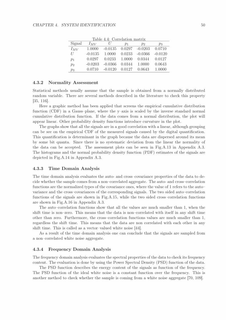
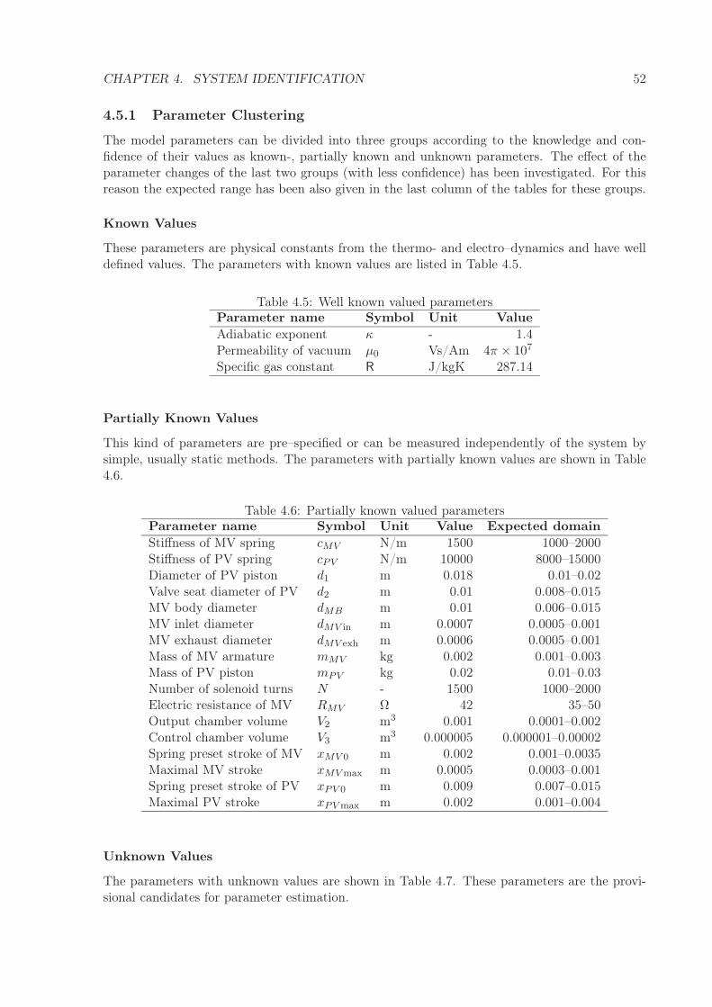
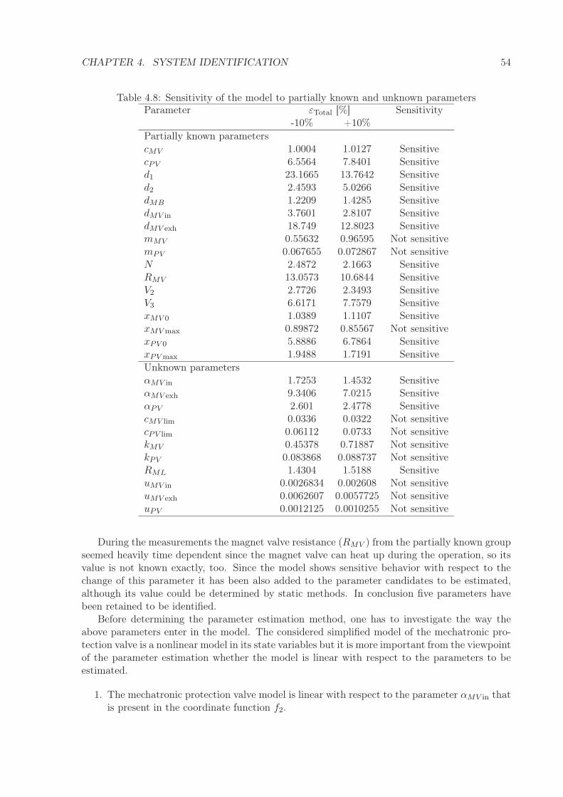
Chapter 4 This part is devoted to the identification of the unknown model parameters andvalidation of the model utilizing laboratory measurements. Sections 4.1–4.2 present themeasurement system with the investigated electro-pneumatic system. The signal qualityof the measurement system is investigated by using statistical methods in Section 4.3.The operation domain of the model is defined in Section 4.4. The model parameters areclassified in order to select the candidates for estimation by sensitivity analysis in Section4.5. The unknown parameters are identified by solving the general dynamic parameterestimation problem in Section 4.6. The identified model is validated against independentmeasurements in Section 4.7.

Chapter 5 The chapter contains the dynamic analysis of the validated model. The investiga-tions are divided into four main parts. The basic properties of the model equations arediscussed in Section 5.1. The properties of the hybrid switching behavior is presented inSection 5.2. The structural dynamical model properties such as state reachability andstate observability are investigated in Section 5.3. The system sensitivity to disturbancesis investigated in Section 5.4. Finally the stability of the open loop system is assessed inSection 5.5.

Chapter 6 This part shows a control design method of a pressure limiting controller for themechatronic protection valve. The designed bang-bang controller structure is discussed inSection 6.4. The controller utilizes a disturbance observer that is designed in Section 6.5.The feedforward module of the controller is given in Section 6.6. The feedback module issynthesized in Section 6.7. The simulation results are presented and discussed in Sections6.8 and 6.9 respectively.


Chapter 7 This chapter contains the final conclusions and the related publications of the thesis,moreover it describes the possible directions for future research.

Appendix A This part of the Appendix contains figures and tables that could not be fit to themain text due to space limitations.

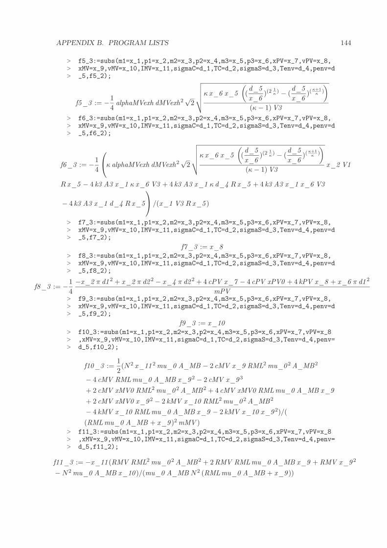
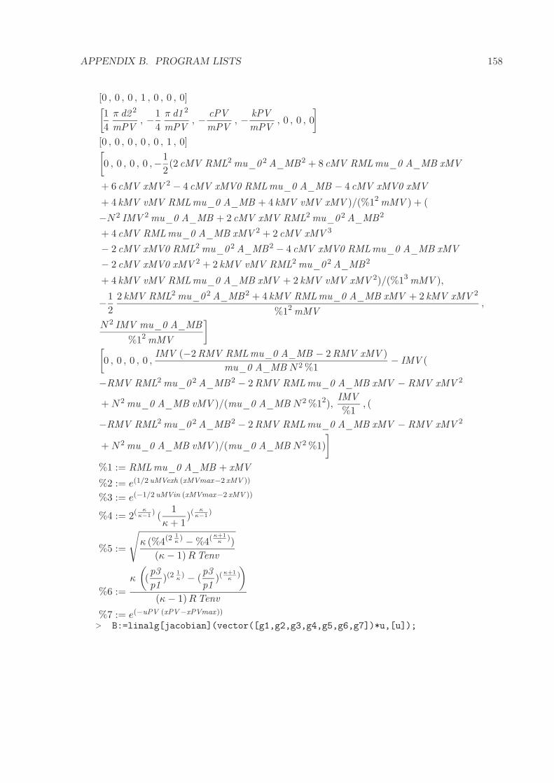
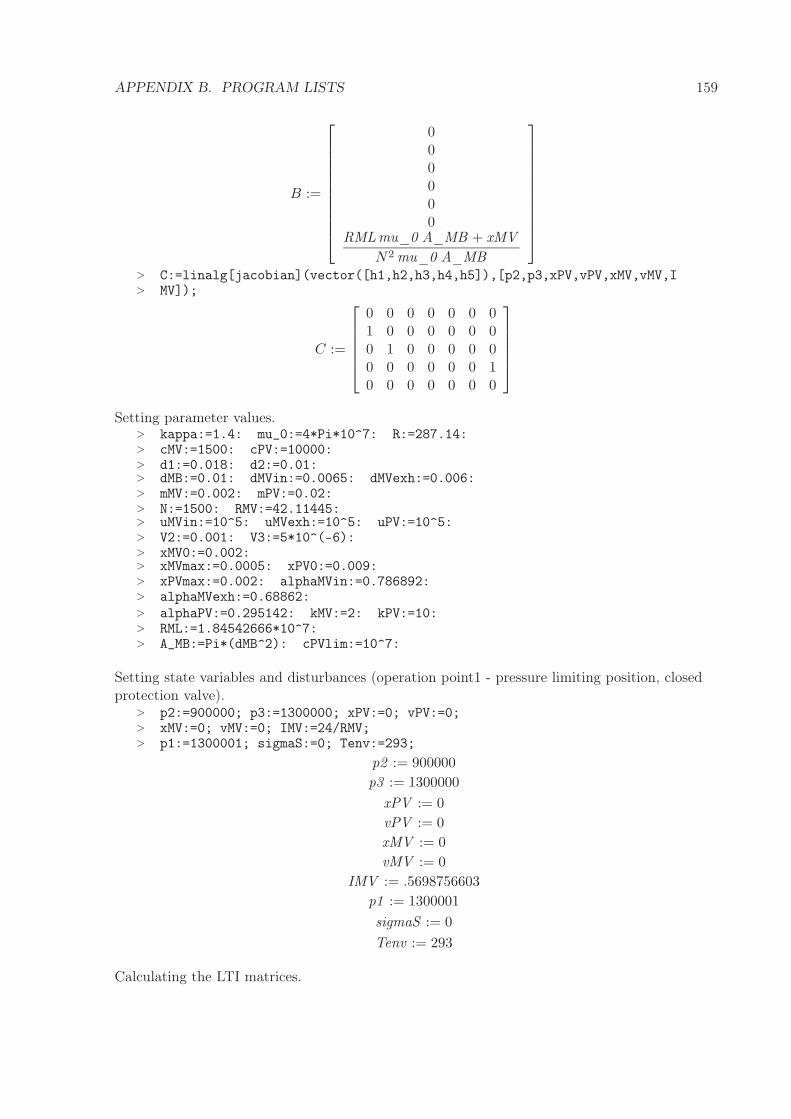
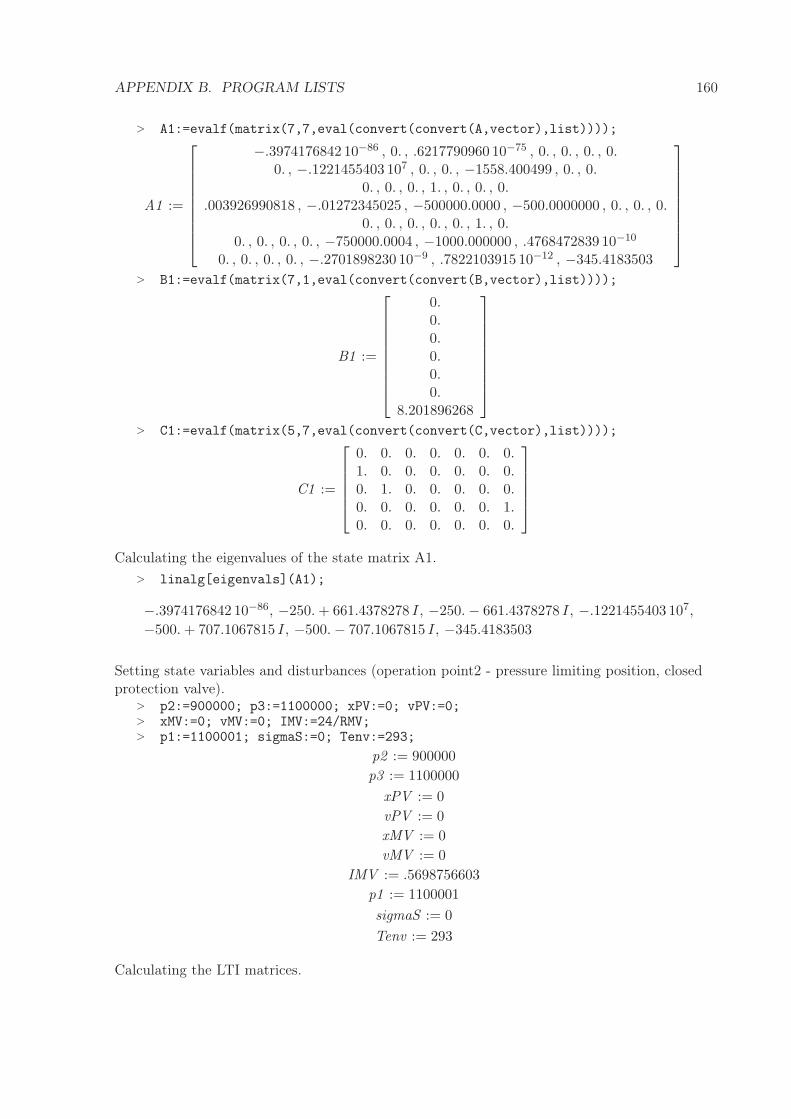
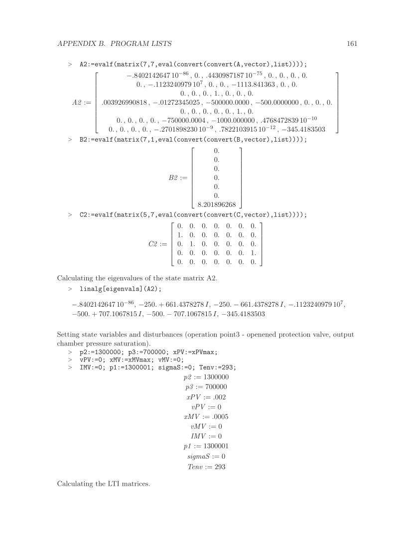
Appendix B This part includes the program lists that has been used for the most importantcontributions of the thesis.


1.5 Nomenclature

The notation list contains all the commonly used symbols and abbreviations throughout thethesis. The units of the physical variables are given in brackets that refer to the SI standard.

Notation of variables and parameters of the mechatronic protection valve

Variables Indices

A area, surface [m2] 0 refers to initial state or vacuumα contraction coefficient [-] 1 refers to input chamberB magnetic induction [Vs/m2] 2 refers to output chamberc specific heat [J/kgK] 3 refers to control chamberc spring coefficient [N/m] ∞ refers to limit in infinityd diameter [m] PV refers to protection valveE energy [J] MV refers to magnet valveE electric field strength [V/m] C refers to compressorI electric current [A] S refers to brake systemF force [N] v refers to constant volumeh specific enthalpy [J/K] p refers to constant pressurek heat transfer coefficient [W/m2K] env refers to environmentk damping coefficient [Ns/m] in refers to inletκ adiabatic exponent [-] out refers to outletλ air flow presence [-] exh refers to exhaustL inductance [Vs/A] max refers to maximumm mass [kg] lim refers to limitationµ permeability [Vs/Am] Σ refers to magnetic resultantN solenoid turns [-] MB refers to magnet valve body – armatureQ heat flux [J/s] ML refers to magnetic loop of constant partsp absolute pressure [Pa] MP refers to magnet valve plug partΦ magnetic flux (magnetic current) [Vs] MF refers to magnet valve frameΨ magnetic linkage [Vs] MJ refers to magnet valve jacketR resistance [electric-Ω; magnetic-A/V] MC1 refers to magnet valve air clearance 1R specific gas constant [J/kgK] MC2 refers to magnet valve air clearance 2σ air flow [kg/s]t time [s]T absolute temperature [K]Θ excitation (magnetic voltage) [A]u cross section factor [-]U voltage [V]U internal energy of gas [J]v speed [m/s]V volume [m3]x stroke [m]

Notation for state space models

d disturbance vector (d: A ⊂ R → D ⊂ Rv)

u input vector (u: A ⊂ R → U ⊂ Rp)

r hybrid mode mapping (r: X ⊂ Rn → R ⊂ N)

x state vector (x: A ⊂ R → X ⊂ Rn)


y = h(x) measured output vector (y: A ⊂ R → Y ⊂ Rm)

z performance output vector (z: A ⊂ R → Z ⊂ Rr)

f(x), g(x), h(x) coordinate functions of the nonlinear modelx = dx

dt time derivative of the state vector x∂f∂x

Jacobi-matrix of the function f : Rn → Rn, x → f(x)

dh = ∂h∂x

gradient vector of the function h: Rn → R

A, B, C, D matrices of the linear model

Acronyms

ADC analogue to digital converterCDF cumulative distribution functionDAC digital to analogue converterEAC electronic air treatment control systemEBS electronic brake systemECU electronic control unitLS least squaresLTI linear time-invariantMIMO multiple-input multiple-outputMPV mechatronic protection valveMV magnet valvePDF probability density functionPSD power spectral densityPV protection valveSISO single-input single-output

Chapter 2

Nonlinear Hybrid Model of the


The aim of this chapter is to construct a systematically developed model of the single mechatronicprotection valve unit.

A model is a simplified description of a real world object for a given application aim. Thereal processes of the modelled object are first translated into mathematical forms which is thensolved. The solution helps the user to understand the real world system better or design anappropriate control or diagnostic method to the corresponding object of the modelling.

The model is prepared using first engineering principles such as thermo–dynamic, mechanicaland electro–magnetic laws. It is then equipped with constitutive equations to obtain a solvableset of equations. This final set is then transformed into the form required or convenient to thegiven application.

The following steps are considered in this chapter for a systematic modelling procedure [35]:

• Description of the system and its boundary. This gives the components that are needed tobe included, all the inputs/outputs that occur on the system boundary and all the processeswithin this boundary

• Definition of the modelling goals that prescribe the aim of the model and the requiredaccuracy.

• Supplying of simplification assumptions that enable to eliminate unimportant phenomenaand thus to obtain simpler mathematic forms.

• Derivation of conservation equations that are the core equations of the model and are basedon first engineering principles.

• Construction of constitutive equations.

• Transformation of the model into standard state space form for control design applications.

11

CHAPTER 2. NONLINEAR HYBRID MODEL 12

2.1 System Definition

The location and the parts of the system to be modelled are given by a top–down investigationprocedure. First the complete architecture of a pneumatic brake system of commercial heavyvehicles is given then we zoom into that in two steps to obtain the object of the modelling, thesingle mechatronic protection valve unit.

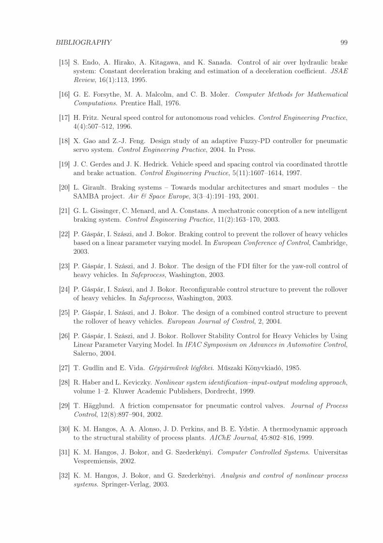
From the air conservation point of view, pneumatic brake systems of commercial vehicles canbe divided into three main hierarchical parts (see Fig.2.1):

1. Air supply subsystem.

2. Air treatment and control subsystem.

3. Air consumption subsystems.

The air supply part has only one operating unit: the compressor (denoted by 3 in Fig.2.1).The air treatment and control part, being in the focus of this thesis, is integrated into one unit(denoted by 4 in Fig.2.1). The air consumption part has several units carrying out the controlof the brake chamber pressure to satisfy the deceleration demand of the driver. Furthermore, airspring and some auxiliary systems (e.g. boosters) belong to the air consumption subsystem, too.

Figure 2.1: Layout of the electro–pneumatic brake system of a towing vehicle (4x2)

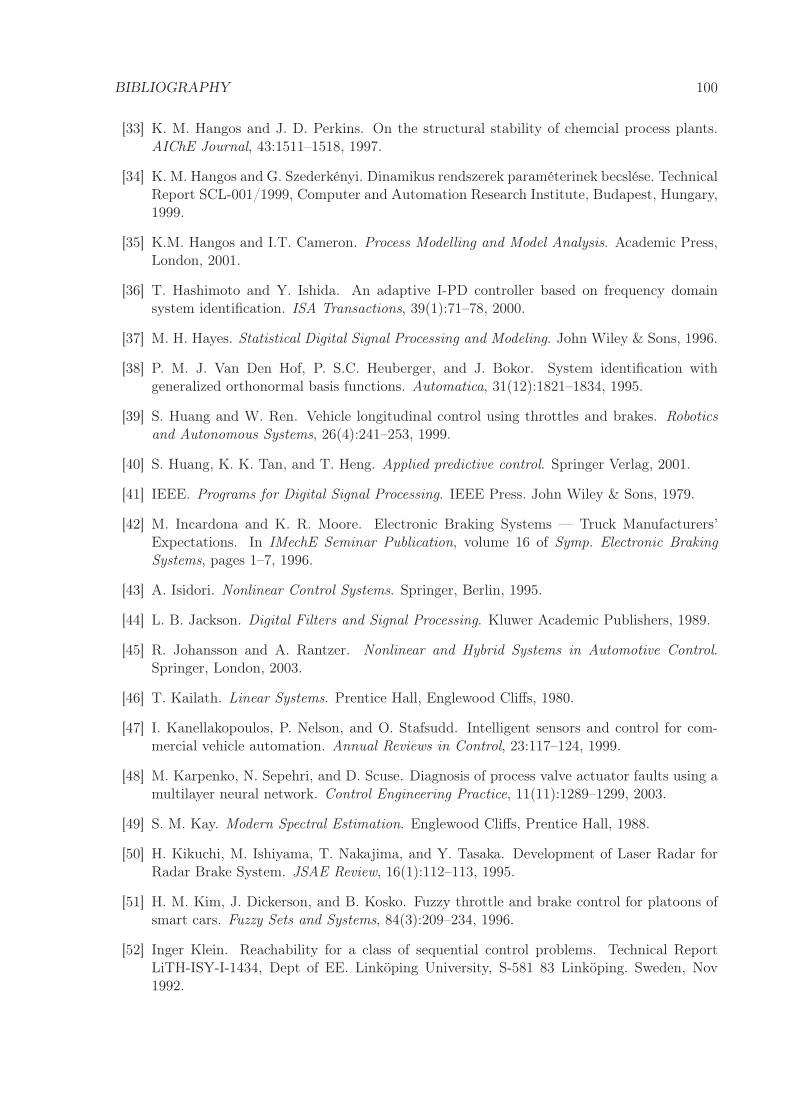
Inside the air treatment and control unit the following three functional components are in-cluded (see Fig.2.2):

1. Electronic control unit (ECU).

2. System pressure and air drying control unit.

3. Air distribution unit.


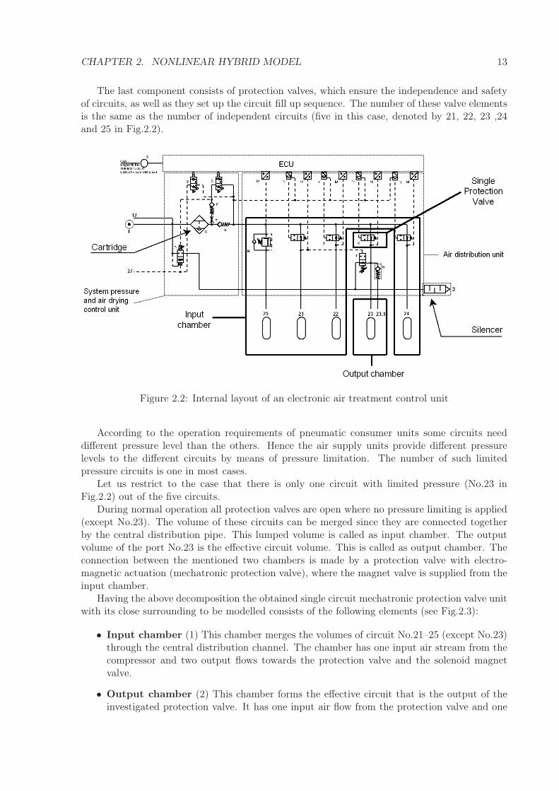
The last component consists of protection valves, which ensure the independence and safetyof circuits, as well as they set up the circuit fill up sequence. The number of these valve elementsis the same as the number of independent circuits (five in this case, denoted by 21, 22, 23 ,24and 25 in Fig.2.2).

Figure 2.2: Internal layout of an electronic air treatment control unit

According to the operation requirements of pneumatic consumer units some circuits needdifferent pressure level than the others. Hence the air supply units provide different pressurelevels to the different circuits by means of pressure limitation. The number of such limitedpressure circuits is one in most cases.

Let us restrict to the case that there is only one circuit with limited pressure (No.23 inFig.2.2) out of the five circuits.

During normal operation all protection valves are open where no pressure limiting is applied(except No.23). The volume of these circuits can be merged since they are connected togetherby the central distribution pipe. This lumped volume is called as input chamber. The outputvolume of the port No.23 is the effective circuit volume. This is called as output chamber. Theconnection between the mentioned two chambers is made by a protection valve with electro-magnetic actuation (mechatronic protection valve), where the magnet valve is supplied from theinput chamber.

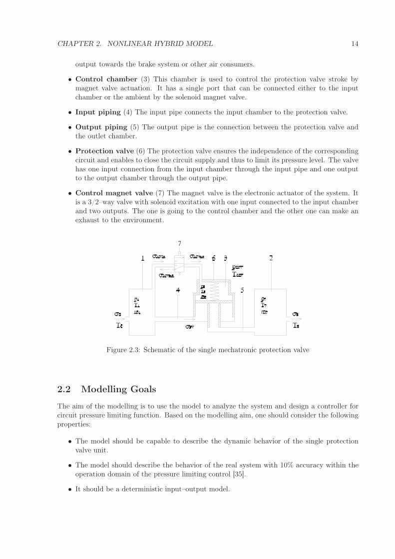
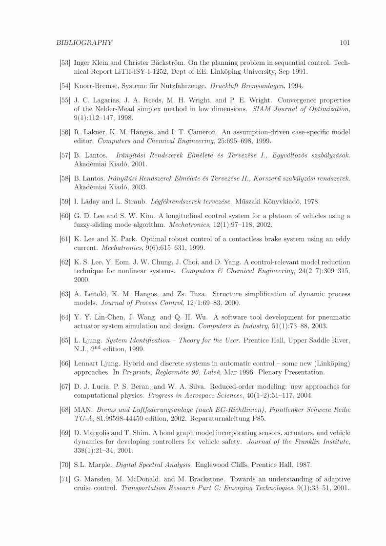
Having the above decomposition the obtained single circuit mechatronic protection valve unitwith its close surrounding to be modelled consists of the following elements (see Fig.2.3):

• Input chamber (1) This chamber merges the volumes of circuit No.21–25 (except No.23)through the central distribution channel. The chamber has one input air stream from thecompressor and two output flows towards the protection valve and the solenoid magnetvalve.

• Output chamber (2) This chamber forms the effective circuit that is the output of theinvestigated protection valve. It has one input air flow from the protection valve and one


output towards the brake system or other air consumers.

• Control chamber (3) This chamber is used to control the protection valve stroke bymagnet valve actuation. It has a single port that can be connected either to the inputchamber or the ambient by the solenoid magnet valve.

• Input piping (4) The input pipe connects the input chamber to the protection valve.

• Output piping (5) The output pipe is the connection between the protection valve andthe outlet chamber.

• Protection valve (6) The protection valve ensures the independence of the correspondingcircuit and enables to close the circuit supply and thus to limit its pressure level. The valvehas one input connection from the input chamber through the input pipe and one outputto the output chamber through the output pipe.

• Control magnet valve (7) The magnet valve is the electronic actuator of the system. Itis a 3/2–way valve with solenoid excitation with one input connected to the input chamberand two outputs. The one is going to the control chamber and the other one can make anexhaust to the environment.

Figure 2.3: Schematic of the single mechatronic protection valve

2.2 Modelling Goals

The aim of the modelling is to use the model to analyze the system and design a controller forcircuit pressure limiting function. Based on the modelling aim, one should consider the followingproperties:

• The model should be capable to describe the dynamic behavior of the single protectionvalve unit.

• The model should describe the behavior of the real system with 10% accuracy within theoperation domain of the pressure limiting control [35].

• It should be a deterministic input–output model.


2.3 Assumptions

When constructing the model of the single mechatronic protection valve system the followingassumptions have been made in order to reduce complexity:

A1. The gas physical properties such as specific heats, gas constant and adiabatic exponent areassumed to be constant over the whole time, pressure and temperature domain.

A2. All chamber pressures are higher or equal to the environment pressure.

A3. The gas in the cambers is perfectly mixed, no spatial variation is considered.

A4. The magnet valve elements are modelled assuming linear magneto–dynamically homoge-neous material.

A5. Heat radiation is neglected.

A6. Compressor air flow, air consumption by the brake system and protection valve air flow areassumed to have non–negative values only, all other airflows can have negative and positivevalues as well depending on the flow direction.

A7. The protection valve piston stroke and its valve seat diameter are assumed to satisfy theinequality: xPV max > d2

4 .

A8. The maximal magnet valve body stroke, inlet and exhaust port diameters are assumed tosatisfy the inequality: xMV max > dMV in

4 + dMV exh

4 .

A9. The magnet valve port cross sections are assumed to satisfy the condition: AMV out ≫AMV in, AMV exh.

A10. Kinetic and potential energy of the gas is neglected.

A11. All pressure forces are neglected on the magnet valve armature.

A12. All gas chambers have invariant volumes.

2.4 Nominal Hybrid Mode

The system contains several parts that exhibit switching– or hybrid behavior. This means thatthe equations, which describe the dynamic behavior of the corresponding subsystem vary accord-ing to certain circumstances [35]. This applies to the conservation and constitutive equations aswell.

To keep the model definition simple the system equations are shown in one dedicated hybridmode only, that is, we fix certain circumstances to obtain a model with well–defined uniquestructure. After that a separate section discusses all the hybrid modes included into the model.

This dedicated hybrid mode corresponds to the fill up procedure of the output chamber (brakecircuit). In this case the input chamber is filled by the compressor meanwhile the output chamberhas lower pressure producing a positive direction air flow through the protection valve, whereits piston stroke has an intermediate position (no stroke limiting). The streaming process issubsonic. The magnet valve has small stroke. The detailed conditions of the nominal hybridmode are shown in Tab.2.1.


Table 2.1: The nominal hybrid modeNo. Condition

1 σMV in ≥ 02 σMV out ≥ 03 0 ≤ xPV < xPV max

4 0 ≤ xMV < dMV exh

45 1 ≥ p2

p1> Πcrit

6 1 ≥ p3

p1> Πcrit

7 1 ≥ penv

p3> Πcrit

2.5 Conservation Equations

The dynamic equations describing the mathematic model of the mechatronic protection valveunit are based on first engineering principles that are applied to predefined balance volumes.

According to assumption A3 the model is a lumped dynamic model, where the balances areobtained as ordinary differential equations.

In order to derive the conservation equations six balance volumes are defined as follows:

1. Input chamber balance volume.

2. Output chamber balance volume.

3. Control chamber balance volume.

4. Protection valve piston balance volume.

5. Magnet valve armature balance volume.

6. Solenoid cross section balance volume.

The balance equations are based on the conservation of mass, energy, momentum and linkagewithin the given balance volume. In most cases open balance volumes are considered where mass,energy or momentum can flow across the boundary surface. One can write a general conservationfor an extensive system property as:

net change ofquantity in time

=

flow inthrough boundary

−

flow outthrough boundary

+

netgeneration

−

netconsumption

.

2.5.1 Conservation of Gas Mass

The general expression for mass balance considering no generation and consumption terms canbe written in word form as:

rate of massaccumulation

=

mass flowin

−

mass flowout

.

It forms the following equation in case of lumped parameter systems with p input and qoutput flows:


dm

dt=

p∑

j=1

σj −q

∑

k=1

σk. (2.1)

The three balance volumes formed by the three gas chambers are denoted by No.1–3 inFig.2.3. The input chamber has one input mass flow from the compressor and two output massflows to the protection valve and the solenoid magnet valve. This gives the following equation:

dm1

dt= σC − σPV − σMV in. (2.2)

The output chamber has one input mass flow from the protection valve and one output massflow to the air consumers (brake system, etc.). The equation reads as:

dm2

dt= σPV − σS . (2.3)

The control chamber has a single port that serves as input according to the flow directionshown in Fig.2.3. The mass balance is obtained:

dm3

dt= σMV out. (2.4)

2.5.2 Conservation of Gas Energy

The general conservation for total energy over a balance volume can be given by:

rate of changeof total energy

=

flow of energyinto the system

−

flow of energyout of the system

+

sourcesor sinks

.

The general form of total energy for a given balance volume with p input and q output flowsis written as [35]:

dE

dt=

p∑

j=1

σj(h + ek + ep) −q

∑

k=1

σk(h + ek + ep) + Q + W, (2.5)

where h, ek and ep denotes the mass specific– enthalpy, kinetic energy and potential energy termsrespectively. Q is the heat source and W is the work term.

According to assumption A10 the potential and kinetic energy terms are neglected. Sinceassumption A12 states that all the three gas balance volumes have constant volumes the workterm is also neglected. In conclusion the simplified energy balance equation is written:

dU

dt=

p∑

j=1

σjhj −q

∑

k=1

σkhk + Q, (2.6)

where the extensive conserved quantity is the internal energy on the left hand side that dominatesthe total energy content of the gas.

The above extensive form of the conservation balance equation should be transformed intoits intensive form, in order to have a measurable intensive variable as its differential variable.For this purpose the chamber pressure has been selected.

The chamber pressure change can be expressed using the definition of the internal energyand the ideal gas equation (pV = mRT ) as follows:


dU

dt=

d (cvmT )

dt=

d(

cvpVR

)

dt=

cvV

R

dp

dt=

V

κ − 1

dp

dt, (2.7)

where

κ =cp

cv. (2.8)

The mass specific enthalpy term h is defined as the product of the coefficient of specific heatat constant pressure and the source side temperature as:

h = cpT. (2.9)

Since this temperature depends on the source side that is depending on the direction of theair flow, this term introduces hybrid or switching behavior (see later in Section 2.7). That givesmany definitions to the same equation that are valid in a given hybrid mode only.

Similarly to the mass balance equations, the same balance volumes are used for the deriva-tion of the energy balance equations. Considering the different input and output air flows andtemperatures that depend on the hybrid mode the input chamber pressure balance can be givenby four equations. In the predefined nominal hybrid mode (when σC ≥ 0, σPV ≥ 0, σMV in ≥ 0)the pressure change in the input chamber is as follows:

dp1

dt=

κR

V1(σCTC − σPV T1 − σMV inT1) +

κ − 1

V1Q1. (2.10)

Similarly, in the given nominal hybrid mode (when σPV ≥ 0, σS ≥ 0) the pressure change inthe output chamber reads as:

dp2

dt=

κR

V2(σPV T1 − σST2) +

κ − 1

V2Q2. (2.11)

Finally, in the given nominal hybrid mode (when σMV out ≥ 0) the following pressure changeis obtained for the control chamber:

dp3

dt=

κR

V3(σMV outT1) +

κ − 1

V3Q3. (2.12)

2.5.3 Conservation of Protection Valve Piston Momentum

Momentum is the product of mass and velocity. The general conservation equation for momentumis written as:

rate of changeof momentum

=

rate of momentuminto the system

−

rate of momentumout of the system

+

sum of all forceson the system

.

The general form of momentum balance volume with p forces acting on the system is writtenas [35]:

dM

dt= Mi − Mo +

p∑

k=1

Fk, (2.13)


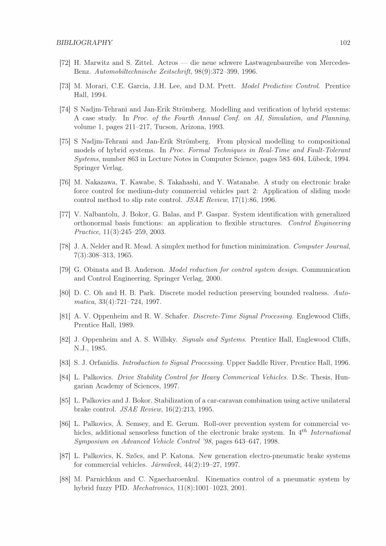
Figure 2.4: The protection valve piston with its close surrounding

where Mi and Mo are the momentum into and out of the system respectively and Fk denotesthe forces acting on the system.

Considering the forces acting on the system generated by the pressure, springs, etc. shownin Fig.2.4 the momentum balance of the protection valve piston is obtained as follows:

d(mPV vPV )

dt= FPV 1 + FPV 2 − cPV (xPV + x0PV ) − kPV vPV − FPV 3 + FPV lim, (2.14)

where FPV 1 and FPV 2 are the forces generated by the input and output chamber pressures.In the equation above there are spring– and damping forces, FPV 3 is the force generated bythe control chamber pressure and finally FPV lim is the stroke limiting force since the piston isintegrated into a housing.

Assuming constant piston mass the equation can be rearranged as follows:

dvPV

dt=

FPV 1 + FPV 2 − cPV (xPV + x0PV ) − kPV vPV − FPV 3 + FPV lim

mPV. (2.15)

The stroke change of the piston is obtained as:

dxPV

dt= vPV . (2.16)

2.5.4 Conservation of Magnet Valve Armature Momentum

Similarly to the momentum balance of the protection valve piston the magnet valve body (ar-mature) balance is derived considering assumption A11 and Fig.2.5.

The obtained momentum balance is as follows:

d(mMV vMV )

dt= FMV − cMV (xMV + x0MV ) − kMV vMV + FMV lim, (2.17)

where FMV is the magnetic force generated by the solenoid. There are spring–, damping– andthe stroke limiting force FMV lim in the above equation.

The rearranged equations are written for armature velocity and position change as:

dvMV

dt=

FMV − cMV (xMV + x0MV ) − kMV vMV + FMV lim

mMV, (2.18)

dxMV

dt= vMV . (2.19)


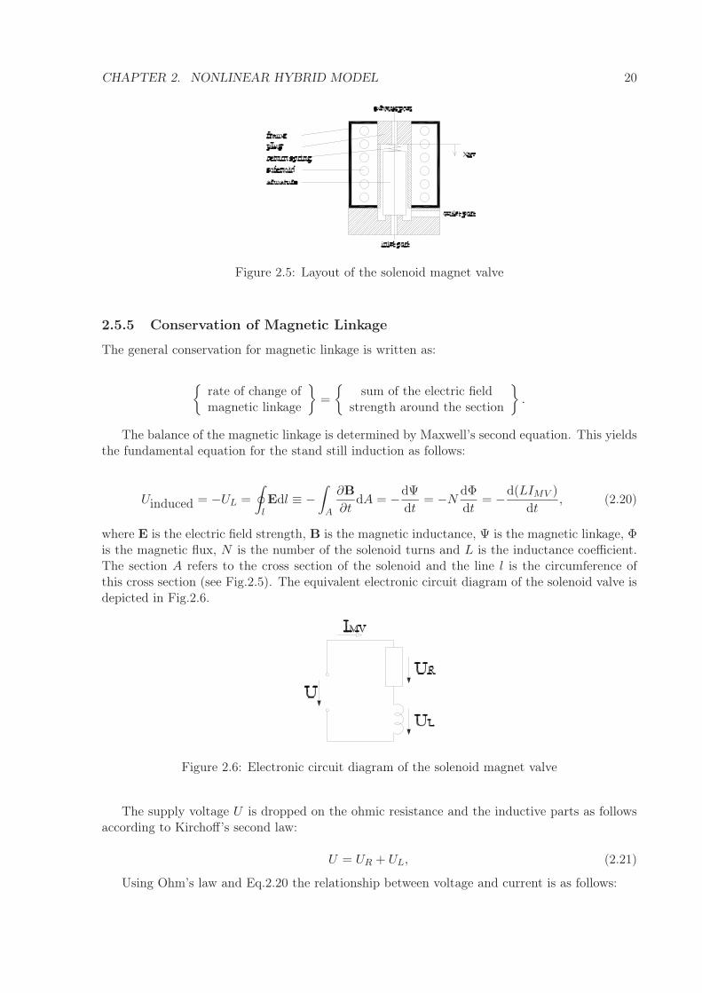
Figure 2.5: Layout of the solenoid magnet valve

2.5.5 Conservation of Magnetic Linkage

The general conservation for magnetic linkage is written as:

rate of change ofmagnetic linkage

=

sum of the electric fieldstrength around the section

.

The balance of the magnetic linkage is determined by Maxwell’s second equation. This yieldsthe fundamental equation for the stand still induction as follows:

Uinduced = −UL =

∮

lEdl ≡ −

∫

A

∂B

∂tdA = −dΨ

dt= −N

dΦ

dt= −d(LIMV )

dt, (2.20)

where E is the electric field strength, B is the magnetic inductance, Ψ is the magnetic linkage, Φis the magnetic flux, N is the number of the solenoid turns and L is the inductance coefficient.The section A refers to the cross section of the solenoid and the line l is the circumference ofthis cross section (see Fig.2.5). The equivalent electronic circuit diagram of the solenoid valve isdepicted in Fig.2.6.

Figure 2.6: Electronic circuit diagram of the solenoid magnet valve

The supply voltage U is dropped on the ohmic resistance and the inductive parts as followsaccording to Kirchoff’s second law:

U = UR + UL, (2.21)

Using Ohm’s law and Eq.2.20 the relationship between voltage and current is as follows:


U = RMV IMV +d(LIMV )

dt. (2.22)

After expansion of the induced voltage term one obtains that:

U = RMV IMV + LdIMV

dt+ IMV

dL

dt, (2.23)

where RMV denotes the ohmic resistance. In Eq.(2.23) dLdt can be expressed as dL

dxMV

dxMV

dt anddL

dxMVcan be written as dL

dRΣ

dRΣ

dxMVso the equation can be rewritten as:

dIMV

dt=

U

L− RMV IMV

L− IMV

L

dL

dRΣ

dRΣ

dxMVvMV , (2.24)

where RΣ is the magnetic resistance of the solenoid magnet valve.

2.6 Constitutive Equations

To complete the above equations some additional algebraic constraints are needed to be definedsuch as transfer rates, property relations, equipment constraints and defining equations for othercharacterizing variables.

2.6.1 Chamber Gas Properties

The temperature of the gas in the chambers is obtained using the ideal gas equation. The inputchamber gas temperature is written:

T1 =p1V1

m1R. (2.25)

Similarly one obtains the gas temperatures in the output and control chambers as follows:

T2 =p2V2

m2R. (2.26)

T3 =p3V3

m3R. (2.27)

The heat transfer in the gas chambers is calculated according to Newton’s heat transfer lawthat gives the following equation for the input chamber:

Q1 = k1A1(T1 − Tenv), (2.28)

where k is the heat transfer coefficient and A is the surface area of the chamber. Similarly theoutput and control chamber heat energy flows are written as:

Q2 = k2A2(T2 − Tenv). (2.29)

Q3 = k3A3(T3 − Tenv). (2.30)


2.6.2 Forces Acting on the Protection Valve Piston

On the upper side the protection valve piston is affected by a cylindrical spring and the controlpressure (p3). On the lower side it is affected by the pressure distribution from the output (p2)and input (p1) chamber pressures (inner circular section – output side and outer ring section –input side). The pressure force acting on the outer ring surface can be written as:

FPV 1 = p1d2

1 − d22

4π. (2.31)

FPV 2 is generated on the inner circular surface:

FPV 2 = p2d2

2π

4. (2.32)

The force of the control chamber pressure is given as:

FPV 3 = p3d2

1π

4. (2.33)

The stroke limiting force of the protection valve piston is modelled as a stiff spring if thestroke exceeds the limits. This introduces three hybrid modes, two limiting positions at thestroke ends and the third one corresponds to the intermediate stroke position. According to theselected nominal hybrid mode the piston is in intermediate position so the stroke limiting forceis zero:

FPV lim = 0. (2.34)

2.6.3 Airflow Properties of the Protection Valve

The streaming cross section of the protection valve is determined by the orifice between thevalve seat and the piston. If the piston stroke is zero (or less) then there is no streaming. Ifthe stroke is above zero the orifice is determined by a cylindrical surface. If there is a big strokethen the orifice is limited by the circular surface of the valve seat. This implies hybrid behavior.According to the nominal hybrid mode with intermediate stroke position (when 0 < xPV ≤ d2/4)the streaming cross section of the protection valve is written as follows:

APV = xPV d2π. (2.35)

The local gas speed in the protection valve at vena contracta is determined by the pressureratio between the two ports of the protection valve since the streaming conditions are subsonicaccording to the nominal hybrid mode. The mass flow through the protection valve consideringthe subsonic conditions is written as:

σPV = αPV APV

√

√

√

√2κ

κ − 1

p1 m1

V1

[

(

p2

p1

) 2

κ

−(

p2

p1

)κ+1

κ

]

, (2.36)

where αPV is the contraction coefficient of the stream.


2.6.4 Forces Acting on the Magnet Valve Armature

Similarly to the protection valve piston stroke limitation the magnet valve stroke limiting forceis modelled as a stiff spring if the stroke exceeds the limits. This introduces three more hybridmodes the same way as already been discussed.

Since the magnet valve has a small but intermediate stroke in the nominal hybrid mode thestroke limiting force is zero.

FMV lim = 0. (2.37)

The magnetic force can be calculated as the partial derivative of the energy of the magneticfield with respect to the stroke as:

FMV = −∂EMV

∂xMV=

Θ2

2R2Σ

dRΣ

dxMV=

(N IMV )2

2R2Σ

dRΣ

dxMV, (2.38)

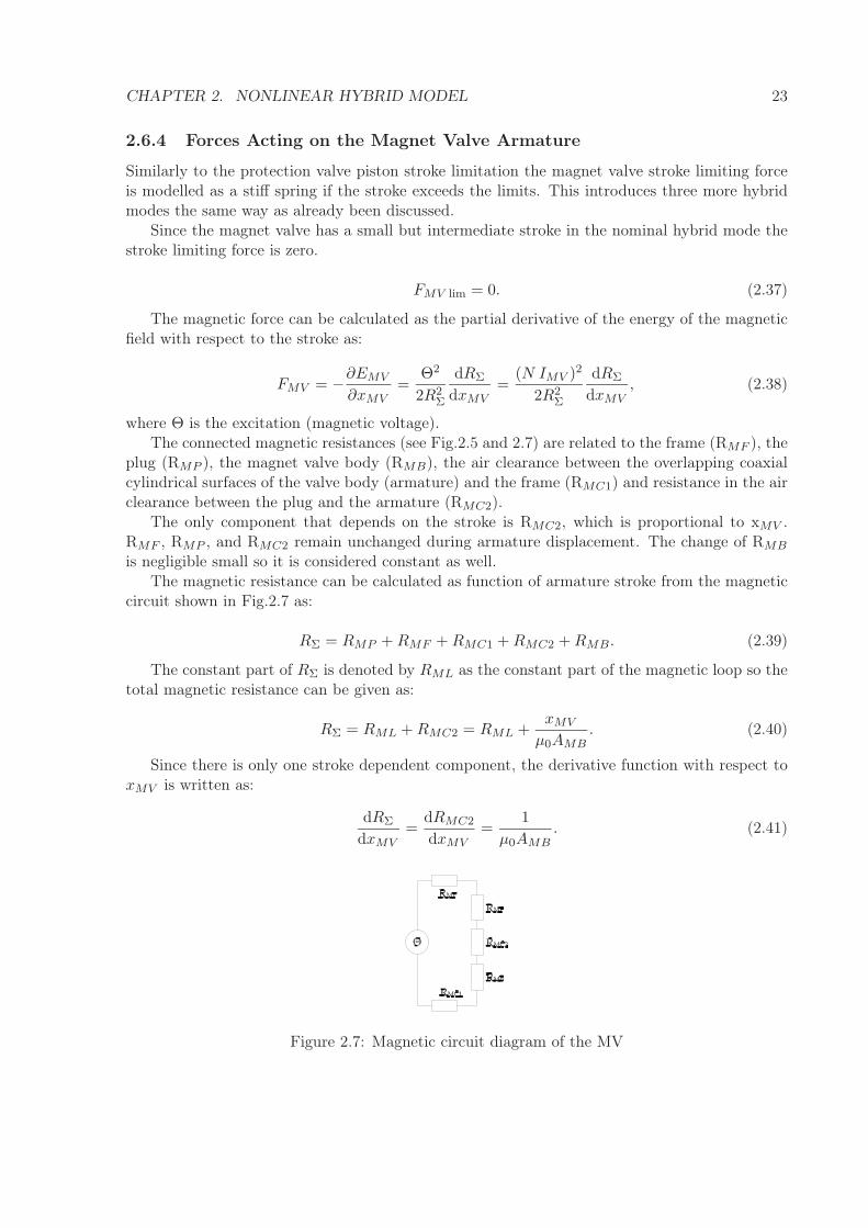
where Θ is the excitation (magnetic voltage).The connected magnetic resistances (see Fig.2.5 and 2.7) are related to the frame (RMF ), the

plug (RMP ), the magnet valve body (RMB), the air clearance between the overlapping coaxialcylindrical surfaces of the valve body (armature) and the frame (RMC1) and resistance in the airclearance between the plug and the armature (RMC2).

The only component that depends on the stroke is RMC2, which is proportional to xMV .RMF , RMP , and RMC2 remain unchanged during armature displacement. The change of RMB

is negligible small so it is considered constant as well.The magnetic resistance can be calculated as function of armature stroke from the magnetic

circuit shown in Fig.2.7 as:

RΣ = RMP + RMF + RMC1 + RMC2 + RMB. (2.39)

The constant part of RΣ is denoted by RML as the constant part of the magnetic loop so thetotal magnetic resistance can be given as:

RΣ = RML + RMC2 = RML +xMV

µ0AMB. (2.40)

Since there is only one stroke dependent component, the derivative function with respect toxMV is written as:

dRΣ

dxMV=

dRMC2

dxMV=

1

µ0AMB. (2.41)

Figure 2.7: Magnetic circuit diagram of the MV


2.6.5 Airflow Properties of the Magnet Valve

The magnet valve streaming cross section relation forms hybrid modes similarly to the protectionvalve streaming cross sections but the magnet valve has two ports and cross section that arerelated to the armature stroke (exhaust and inlet ports).

This results in five hybrid modes considering the assumption A8, which means that there isa particular stroke when both cross sections are limited by circular sections.

According to the selected nominal hybrid mode an intermediate armature position applies(see Fig.2.7), where the exhaust cross section is given by a cylindrical surface:

AMV exh = xMV dMV exhπ. (2.42)

The inlet port section is limited in this position by a circular section as:

AMV in =d2

MV inπ

4. (2.43)

According to the magnet valve streaming cross section assumption A9, the control chamberpressure can be used as internal pressure level inside the magnet valve. This means that the inletand exhaust air flows are defined by the pressure ratio between the control chamber pressureand the corresponding port pressures. Moreover the outlet airflow is determined by the followingalgebraic equation:

σMV out = σMV in − σMV exh. (2.44)

The nominal hybrid mode selection assumes subsonic streaming conditions so the exhaustairflow of the magnet valve is written as:

σMV exh = αMV exhAMV exh

√

√

√

√2κ

κ − 1

p3 m3

V3

[

(

penv

p3

) 2

κ

−(

penv

p3

)κ+1

κ

]

, (2.45)

where αMV exh is the magnet valve exhaust port contraction coefficient. The inlet air flow of themagnet valve is:

σMV in = αMV inAMV in

√

√

√

√2κ

κ − 1

p1 m1

V1

[

(

p3

p1

) 2

κ

−(

p3

p1

)κ+1

κ

]

, (2.46)

where αMV in is the magnet valve inlet port contraction coefficient.

2.6.6 Electro–Magnetic Relations

The inductance of the solenoid magnet valve is written as the following equality of the numberof solenoid turns and the magnetic resistance:

L =N2

RΣ. (2.47)

Its derivative with respect to the magnetic resistance is given as follows:

dL

dRΣ= −N2

R2Σ

. (2.48)


2.7 Hybrid Items

The above defined equations describe the system in a special hybrid mode only. To generalizethe model all of the cases have to be collected that describe the changes in the model equationsand their domains.

The model includes three subsystem types that exhibit hybrid behavior. These are as followswith the included components:

• Enthalpy terms in the pressure equations

– Inlet chamber (2 hybrid modes)

– Control chamber (2 hybrid modes)

• Streaming cross-sections and stroke limiting forces

– Protection valve (3 hybrid modes)

– Magnet valve (5 hybrid modes)

• Air flow terms

– Protection valve (2 hybrid modes)

– Magnet valve (4 and 2 hybrid modes)

Streaming cross–section and valve stroke limiting subsystems are dependent from each othercorresponding the same stroke. For this reason they are listed above together.

2.7.1 Gas Enthalpy

According to Eq.(2.9) the enthalpy term considers the source side gas temperature wherefromthe stream is coming (gas energy inherited with the stream). This implies different temperatureexpressions depending on the streaming direction.

The input chamber has three ports that realizes air flow into or out of the chamber. Assump-tion A6 states that the compressor– and protection valve air flows have non–negative values sothe input chamber has one port only where the enthalpy term is influenced by the flow direction.

Let us denote the temperature multiplier of σMV in by TMV in in Eq.(2.10). The hybrid modesof the input chamber gas energy equation are shown in Tab.2.2 including the correspondingtemperature expressions and the conditions.

Table 2.2: Hybrid modes of the input chamber gas energy equationName Condition TMVin

HM1a σMV in ≥ 0 T1

HM2a σMV in < 0 T3

The output chamber has two ports that realizes air flow into or out of the chamber. Assump-tion A6 states that both flows have non-negative values so the output chamber has no portswhere the enthalpy term is influenced by the flow direction.

The control chamber has one port only that realizes air flow into or out of the chamber. Letus denote the temperature multiplier of σMV out by TMV out in Eq.(2.12). The hybrid modes ofthe control chamber gas energy equation are shown in Tab.2.3.


Table 2.3: Hybrid modes of the control chamber gas energy equationName Condition TMVout

HM1b σMV out ≥ 0 T1

HM2b σMV out < 0 T3

2.7.2 Cross-sections and Stroke Limiting

The streaming cross section expressions and stroke limiting forces are depending on the strokeof the corresponding valve unit this way they are dependent hybrid modes regarding the samevalve unit.

The protection valve streaming cross section is zero if the piston is closed. If there is a positivestroke the cross section is determined by a cylindrical surface area. If there is a big stroke thenthe cross section is limited by the circular area of the valve seat. Assumption A7 ensures thatsuch a big stroke does not occur due to stroke limitation. That implies two hybrid modes dueto the streaming cross section.

The stroke limitation is modelled by stiff springs if the stroke exceeds the limits. In interme-diate position this limiting force is absent. In conclusion the protection valve has three hybridmodes that are stroke dependent due to the streaming cross section and stroke limiting forceequations. The hybrid modes of the protection valve streaming cross section and stroke limitingforce equations are shown in Tab.2.4.

Table 2.4: Hybrid modes of the protection valve cross section and limiting forcesName Condition APV FPVlim

HM1c xPV < 0 0 −cPV limxPV

HM2c 0 ≤ xPV < xPV max xPV d2π 0HM3c xPV ≥ xPV max xPV d2π −cPV lim(xPV − xPV max)

The magnet valve has similar properties related to the streaming cross section and strokelimiting. The stroke limiting works exactly the same. The difference with cross sections is thatit has two ports where the streaming cross section is stroke dependent. Assumption A8 givesthat there are five hybrid modes due to the cross sections. Let x′

MV = xMV max − xMV denotethe complementary stroke of the magnet valve. The hybrid modes of the magnet valve streamingcross section and stroke limiting force equations are shown in Tab.2.5.

Table 2.5: Hybrid modes of the magnet valve cross sections and limiting forcesName Condition AMVin AMVexh FMVlim

HM1d xMV < 0d2

MV inπ

40 −cMV limxMV

HM2d 0 ≤ xMV < dMV exh

4

d2MV in

π4 xMV dMV exhπ 0

HM3d dMV exh

4≤ xMV < xMV max − dMV in

4

d2

MV inπ

4

d2MV exh

π4 0

HM4d xMV max − dMV in

4≤ xMV < xMV max x′

MVdMV inπ

d2MV exh

π4 0

HM5d xMV max ≤ xMV 0d2

MV exhπ

4 cMV limx′

MV

2.7.3 Air flows

The air flow on a port between two chambers is governed by the pressure ratio and four casescan be distinguished that can be subsonic and sonic in both directions (assuming that no Laval


geometry is met). The sonic streaming conditions are determined by the critical pressure ratio,which can be written as:

Πcrit =

(

2

κ + 1

) κκ−1

. (2.49)

Assumption A6 states that the protection valve air flow is considered as a non–negative airflow. This implies two hybrid modes only both in the same streaming direction. There is onlyone part in Eq.(2.36) that depends on the hybrid mode: the pressure ratio under the exponents.The corresponding hybrid modes are shown in Tab.2.6.

Table 2.6: Hybrid modes of the protection valve air flowName Condition Pressure ratio

HM1e 1 ≥ p2

p1> Πcrit

p2

p1

HM2e p2

p1≤ Πcrit Πcrit

Similarly the magnet valve input air flow has hybrid modes but four pieces due to the possiblenegative direction. So there are three parts of Eq.(2.46) that depend on the hybrid mode: thesign of the whole expression (streaming direction), the pm

V expression that originates from thesource side gas density and the pressure ratio under the exponents. Its hybrid modes are shownin Tab.2.7.

Table 2.7: Hybrid modes of the magnet valve input air flowName Condition Sign Density term Pressure ratio

HM1f 1 ≥ p3

p1> Πcrit + p1m1

V1

p3

p1

HM2f p3

p1≤ Πcrit + p1m1

V1Πcrit

HM3f 1 > p1

p3≥ Πcrit − p3m3

V3

p1

p3

HM4f p1

p3< Πcrit − p3m3

V3Πcrit

According to assumption A2 the magnet valve exhaust air flow is always non–negative so thesign of Eq.(2.45) is always positive and the density term is also not changed. The only changingpart is the pressure ratio. The hybrid modes of the magnet valve exhaust air flow are shown inTab.2.8.

Table 2.8: Hybrid modes of the magnet valve exhaust air flowName Condition Pressure ratio

HM1g 1 ≥ penv

p3> Πcrit

penv

p3

HM2g penv

p3≤ Πcrit Πcrit

2.8 Model Equations in State Space Form

The most convenient model representation for analysis and control design purposes is the statespace realization. This requires that the model variables are arranged in vector format. Thefollowing five system variables are composed.

State Vector of the Nonlinear Model From the conservation equations the state vector iscomposed of their differential variables as:


x =[

m1 p1 m2 p2 m3 p3 xPV vPV xMV vMV IMV

]T.

Disturbance Vector The uncontrollable inputs form the disturbance vector including com-pressor flow rate and its gas temperature, brake system consumption, ambient temperature andpressure respectively:

d =[

σC TC σS Tenv penv

]T.

Input Vector The control input vector includes one member only, which is the excitation voltageof the MV:

u = [U ] .

Measured Output The measurable state variables and disturbances are formed as measuredoutput including the input–, output– and control chamber pressures, the solenoid current andcircuit air consumption presence as discrete variable:

y =[

p1 p2 p3 IMV λS

]T.

Performance Output The performance output is the output chamber pressure:

z = [p2] .

2.8.1 State Equation

For sake of simplicity the state space equation is given for the same nominal hybrid mode asused at the equation definition.

Substituting the constitutive equations into the differential conservation balances the follow-ing state space model is obtained:

dx

dt= f(x,d, r) + g(x)u, (2.50)

where r: Rn → N is a piecewise constant switching function mapping from the state space toN. The integer set N is finite, i.e. N = 1, 2, . . . , n, where n =

∏gi=a ni is the total number

of hybrid modes and ni is the number of the individual hybrid modes of a subsystem (n =2 × 2 × 3 × 5 × 2 × 4 × 2 = 960). Moreover, the values of r(x) are composed by the conditionsdefined in Tables 2.2–2.8. Eq.(2.50) can be expanded as:

m1

p1

m2

p2

m3

p3

xPV

vPV

xMV

vMV

IMV

=

f1(x,d, r)f2(x,d, r)f3(x,d, r)f4(x,d, r)f5(x,d, r)f6(x,d, r)f7(x,d, r)f8(x,d, r)f9(x,d, r)f10(x,d, r)f11(x,d, r)

+

0000000000

RML+xMV

µ0AMB

N2

[U ] . (2.51)


Let the value of the switching function mapping r be 1 for the nominal hybrid mode. Thenonlinear state functions with all constitutive relations substituted for the nominal hybrid modeare obtained as (the entries that depend on the hybrid operation modes are denoted by blue):

f1(x,d, 1) = σC − αPV d2πxPV ξ(p1, p2, m1) − αMV ind2

MV inπ

4ξ(p1, p3, m1), (2.52)

f2(x,d, 1) =κσCTCm1R

2 − κRαPV d2πxPV ξ(p1, p2, m1)p1V1

Rm1V1+

k1A1κp1V1 − k1A1κTenvRm1 − k1A1p1V1 + k1A1TenvRm1

Rm1V1−

κRαMV ind2MV inπξ(p1, p3, m1)p1V1

4Rm1V1, (2.53)

f3(x,d, 1) = αPV d2πxPV ξ(p1, p2, m1) − σS , (2.54)

f4(x,d, 1) =κRαPV d2πxPV ξ(p1, p2, m1)p1V1m2 − κRσSp2V2m1 + k2A2m1κp2V2

Rm1m2V2−

k2A2m1κTenvRm2 + k2A2m1p2V2 − k2A2m1TenvRm2

Rm1m2V2, (2.55)

f5(x,d, 1) = αMV ind2

MV inπ

4ξ(p1, p3, m1) − αMV exhdMV exhπxMV ξ(p3, penv, m3), (2.56)

f6(x,d, 1) =k3A3m1κp3V3 − k3A3m1κTenvRm3 − k3A3m1p3V3 + k3A3m1TenvRm3

m3V3m1R+

κπp1V1Rm3αMV ind2MV inξ(p1, p3, m1) − 4κπp1V1Rm3αMV exhdMV exhxMV ξ(p3, penv, m3)

4m3V3m1R, (2.57)

f7(x,d, 1) = vPV , (2.58)

f8(x,d, 1) =p1

(

d21 − d2

2

)

π + p2d22π − p3d

21π − 4cPV (xPV + x0PV ) − 4kPV vPV + 0

4mPV, (2.59)

f9(x,d, 1) = vMV , (2.60)

f10(x,d, 1) =

N2IMV2

2(RML+xMV

µ0AMB)2µ0AMB

− cMV (xMV + x0MV ) − kMV vMV + 0

mMV, (2.61)

f11(x,d, 1) =IMV vMV

(RML + xMV

µ0AMB)µ0AMB

−RMV IMV (RML + xMV

µ0AMB)

N2, (2.62)


where

ξ(p1, p2, m1) =

√

√

√

√

√

2κp1m1

(

(

p2

p1

) 2

κ −(

p2

p1

)κ+1

κ

)

(κ − 1)V1,

ξ(p1, p3, m1) =

√

√

√

√

√

2κp1m1

(

(

p3

p1

) 2

κ −(

p3

p1

)κ+1

κ

)

(κ − 1)V1,

ξ(p3, penv, m3) =

√

√

√

√

√

2κp3m3

(

(

penv

p3

) 2

κ −(

penv

p3

)κ+1

κ

)

(κ − 1)V3.

2.8.2 Output Equation

Since the output is linear with respect to the state vector, the measured output is written as thefollowing state–affine equation:

y = Cx + e(d). (2.63)

After the substitution the result reads as follows:

y =

0 1 0 0 0 0 0 0 0 0 00 0 0 1 0 0 0 0 0 0 00 0 0 0 0 1 0 0 0 0 00 0 0 0 0 0 0 0 0 0 10 0 0 0 0 0 0 0 0 0 0

x +

0000

sgn(σS)

. (2.64)

The performance output is generated from the measured output by the following simpleequation:

z =[

0 1 0 0 0]

y. (2.65)

The Maple V program about reconstruction of the state space realization can be found inthe Appendix B.1.

2.9 Model Verification

The verification of the developed nonlinear model is performed by extensive simulation experi-ments using MATLAB/SIMULINK model against engineering intuition and operation experienceon the quantitative behavior of the system.

To obtain the model solutions the stiff ODE23s solver (Modified Rosenbrock formula [98])with variable step size has been used. The relative tolerance setup of the solver was 10−8.

The simulation calculations consider three typical operating cases. Two of them have beenexecuted without modulation of the magnet valve. The third one investigates the magnet valveexcitation in order to see the effect of magnet valve activation on the output chamber pressure.The model parameter setup can be found in Tab.A.1. in the Appendix A.1.


2.9.1 System fill up process

The fill up process is simulated with constant compressor airflow and constant filling gas tem-perature (accomplished by intercooling). The initial state vector is as follows:

x0 =[

0.575 6 · 105 1.19 · 10−3 105 5.94 · 10−6 105 0 0 5 · 10−4 0 0]T

.

The initial disturbance vector is considered as:

d0 =[

10−2 293 0 293 105]T

.

The dynamic response functions are shown in the Appendix A.1 (See Fig.A.1). The responsesagree with the engineering expectations: the input chamber pressure increased, thereafter reach-ing the dynamic opening pressure of the protection valve the valve stroke increases and herebythe output chamber pressure increases as well.

2.9.2 Circuit defect situation

This case has been simulated with a constant diameter leakage in the circuit (output chamber)to the environment pressure of 105 Pa starting from the common pressure level of 6 · 106 Pa. Noinput side airflow has been considered. The initial state vector is as follows:

x0 =[

0.57 6 · 105 7.13 · 10−3 6 · 105 5.94 · 10−6 105 2 · 10−3 0 5 · 10−4 0 0]T

.


d0 =[

0 293 0 293 105]T

.

In this case the brake system consumption term (σS) in the disturbance vector is a functionof output chamber gas mass and pressure for the subsonic case as follows:

σS = αSAS

√

√

√

√

2κ

κ − 1

p2 m2

V2

[

(

penv

p2

) 2

κ

−(

penv

p2

)κ+1

κ

]

, (2.66)

where the contraction coefficient (αS) is 0.8 and the streaming cross section (AS) is given by a5 mm diameter hole. In sonic case the pressure ratio penv

p2is to be substituted by the critical

pressure ratio given in Eq.(2.49).The dynamic response functions are shown in the Appendix A.1 (See Fig.A.2). The input

and output chamber pressures decreased as expected. By reaching the dynamic closing pressureof the protection valve the valve stroke decreases and finally it closes so the input chamber isprotected against the damaged circuit.

2.9.3 Circuit pressure limiting

This case has been investigated with zero compressor charge. The high pressure input chamberfills the circuit that is pressure limited when the magnet valve becomes activated. The magnetvalve is activated for constant 90 ms intervals after 90 ms deactivation time. The initial statevector is as follows:

x0 =[

1.24 1.3 · 106 8.32 · 10−3 7 · 105 7.72 · 10−5 1.3 · 106 0 0 0 0 0.57]T

.



d0 =[

0 293 0 293 105]T

.

The dynamic response functions are shown in the Appendix A.1 (See Fig.A.3). As seen inthe figure the magnet valve releases after a certain retardation time and exhausts the controlchamber. By this means the protection valve opens and fills the circuit. After a new solenoidexcitation the control chamber is filled up again and the protection valve closes. This is arealization of the circuit pressure limiting cycle.

2.10 Summary

In this section the dynamic model of the mechatronic protection valve has been derived system-atically that satisfies simplifying assumptions. The model has two main parts as follows:

• Conservation equations for gas mass and energy, momentum and magnetic linkage. Theseequations are composed for six predefined balance volumes, where the characterizing exten-sive and intensive quantities are perfectly mixed. The conservation balance equations forma set of nonlinear ordinary differential equations. The presented model contains elevensuch equations.

• The algebraic part of the model contains all relationships to make the model complete.

– The first part of the constitutive equations contain all required equations for thechamber gas properties such as the ideal gas equation and the heat transfer law.

– The second part gives all the unknown forces acting on the protection valve piston.These forces are partly generated by gas pressures and the rest is the stroke limitingforce.

– The third part defines the air flow properties of the protection valve including thestreaming cross sections and flow rates.

– The fourth part defines the unknown forces acting on the magnet valve armature.There are two types of forces: the magnetic– and the stroke limiting force.

– The fifth part gives the air flow properties of the magnet valve with the streamingcross sections and flow rates.

– The last sixth part gives magnetic property relations for the inductance and its deriva-tive with respect to the armature stroke.

The model includes several parts that exhibit mode switching or hybrid behavior. There arethree groups of these parts as follows:

• Enthalpy terms

• Streaming cross sections and stroke limiting forces

• Air flow terms

It has been shown that the dynamic model of the mechatronic protection valve is given by aset of differential–algebraic equations where all the algebraic equations can be substituted intothe differential ones. This equation has a special form given by Eqs.(2.50) and (2.64) with 11state–, 1 input–, 5 disturbance– and 5 output variables. The model has been verified againstengineering expectations.

Chapter 3

Model Simplification

Dynamic system models derived from systematic modelling approaches are sometimes too de-tailed and complex for control purposes. A model for control purpose should retain all majordynamic characteristics of the real plant (such as its stability and main time constants) but omitall details that are weakly represented in the state variables and not related to the control aims.

Therefore a systematically derived model using first engineering principles should often besimplified by reducing the dimension of its state vector and the complexity of its equation formby reducing the number of its parameters using engineering judgement and operating experienceabout the qualitative and quantitative behavior of the real world system.

There are several methods proposed in the literature for performing model simplification andreduction in different ways to obtain a model with suitable size and complexity. These methodscan be classified based on the underlying engineering knowledge used during model simplification.

The so called model reduction methods are entirely of black–box type: they apply statetransformations to find out which combinations of the original state variables do not contributesignificantly to the input–output behavior of the system and thus can be omitted. An exampleis the well–known modred procedure in MATLAB for LTI state space models [35, 114].

The other class, called model simplification uses engineering insight and operation experienceto leave out state variables to be omitted based on the dynamics of the original state variableswith physical meaning. For example Leitold, Hangos and Tuza proposed a graph–theoreticmethod for structure simplification of lumped dynamic process models [35, 63].

The dynamic model presented in the previous chapter contains 11 state–, 5 disturbance–,1 input-, 5 output variables, complex equations forms and many hybrid modes. This modelis capable to describe the dynamic processes of the mechatronic protection valve but it is toocomplex for control design purposes.

The aim of this chapter is to establish a systematic approach to model simplification oflumped parameter nonlinear state space models that respects to pre–defined performance criteriaconsidering the application aim and is based on physical insights. Then this method is appliedto the model derived in the previous chapter.

This chapter describes the following items related to model simplification:

• Definition of a systematic model simplification approach.

• Finding a proper decision making method that considers the application aim of controldesign for circuit pressure limiting.

• Simplification of the mechatronic protection valve model to obtain a lower order model.

• Description of the final simplified state space model of the mechatronic protection valve.

33

CHAPTER 3. MODEL SIMPLIFICATION 34

3.1 The Model Simplification Approach

A dynamic state space model (the simplified model) is considered simpler than another (thedetailed one) with the same set of input- and output variables, if

• the number of its state variables is less than that of the detailed one, and/or

• the algebraic form of its model equations is simpler, together with the number of the modelparameters being less than that of the corresponding model elements in the detailed model.

Model simplification is performed by applying model simplification assumptions [35] to thedynamic model. A model simplification assumption is formally described by a triplet of a modelelement (e.g. a model parameter), an operation (say “=”) and a constant or another modelelement. A simple example is a = 0, where a is a model parameter.

3.1.1 The Structure of the Model Elements

Before attempting to simplify a model that is systematically derived from first engineering prin-ciples, one has to consider the hierarchy of the model elements [56]. A dynamic model can beseen as a hierarchically structured set of the following model elements:

• balance volumes over which conservation balances are constructed (the highest level),

• balance equations,

• terms in balance equations corresponding to mechanisms,

• constitutive equations,

• variables and parameters (the lowest level)

If one makes a simplification assumption to any of the model elements that will influence all theother elements on the lower level(s) that are related to it. For example, leaving out a balancevolume from a model implies to leave out all the balance equations, their terms, constitutiveequations, variables and parameters that belong to that particular balance volume.

Two simplifying assumptions are not related if they are hierarchically independent, i.e. theyhave no common elements in their sub-hierarchy. Naturally, one tries to perform model simpli-fication by applying

• not related assumptions,

• assumptions in their descending order of hierarchy levels, i.e. to apply the most influentialassumption first.

3.1.2 Sensitivity analysis

Another useful and necessary preparatory step of model simplification is to carry out sensitivityanalysis [35] of model parameters that are multiplicative factors of the influential model elements(for example cross sections or characteristic volumes) to see their effect on the input–outputbehavior of the system. If any of such effect is negligible then one can consider the correspondingmodel element as a potential target of model simplification.

This way one can combine engineering insight to the system which is highly domain specificwith empirical (numerical) analysis of the model to be simplified.


3.1.3 Methodology

The systematic method for model simplification consists of the following conceptual steps.

1. Test case selectionThe test cases to be used as reference cases for model simplification are determined basedon the desired use of the model and its operation domain. These test cases should havecharacteristic samples from the entire operation domain and capture the most importantdynamic behavior the system is able to produce. Reference inputs are selected and referenceoutput response to these inputs are generated using the detailed model (i.e. the model tobe simplified) under the test case conditions.

2. Decision criterion selectionThe modelling goal determines the desired accuracy of a model developed for a givenpurpose. Two models have the same performance with respect to a modelling goal, if theirinput–output behavior is the same within that accuracy. The accuracy is then usuallyspecified in terms of a tolerance limit for a signal norm applied to the difference betweenthe output response of the detailed and simplified models to the same reference input. Asimplification is then acceptable with respect to a modelling goal, if the simplified modelproduces the same output as the detailed one within the prescribed accuracy.

‖yorig − ysimpl‖ ≤ ε. (3.1)

3. SimplificationHaving the test cases and the decision criterion, simplifications are carried out step–by–steprepeating the same cycle as follows:

3.1 Select a simplification step based on engineering judgement and perform the modelsimplification to get a simplified model,

3.2 Generate the output response with the simplified model and perform the comparisonwith the response of the detailed model in the test cases,

3.1 Decide on the acceptance of the simplification step based on the decision criterion.

3.1.4 General Applicability

This section is devoted to give the conditions of applying the above described model simplificationmethod in general cases. The necessary preparatory steps that one should perform on the actualsystem are as follows:

• Construct the model hierarchy structure diagram.

• Perform model parameter sensitivity analysis to pre–select model elements from the hier-archy to be omitted.

• Define model performance criteria that is used as decision criterion selection in accordancewith the application aim.

The model hierarchy diagram is automatically obtained if the model is derived by a systematicmodelling procedure by using first engineering principles. This ingredient makes it possible toapply a top–down simplification procedure. The model hierarchy of the detailed mechatronicprotection valve model with balancevolume, equation and mechanism layers is shown in Fig.3.1.



Model

Input chamber balance volume

Output chamber balance volume

Control chamber balance volume

Protection valve piston balance volume

Magnet valve armature balance volume

Solenoid section balance volume

Mass balance

Energy balance

Mass balance

Energy balance

Mass balance

Energy balance

Momentum balance

Momentum balance

Magnetic linkage balance

Con- vective terms

Source /sink term

Con- vective terms

Con- vective terms

Source /sink term

Con- vective terms

Con- vective terms

Source /sink term

Con- vective terms

Pressure terms

Spring term

Damping term

Stroke limiting

term

Magnetic term

Spring term

Damping term

Stroke limiting

term

Source term

Ohmic term

Induc- tive term

Figure 3.1: Hierarchy of the detailed mechatronic protection valve model

The mechanisms introducing hybrid behavior are depicted by dashed line while the others bycontinuous line.

The second ingredient is the result of model parameter sensitivity analysis that gives theparameters and terms in the model equations that have negligible effect on the dynamic behavior.This analysis complements and supports the needed engineering insight on which component arethe candidates for elimination or complexity simplification. The parameter sensitivity analysisof the mechatronic protection valve model is executed to find the most influencing model parts.Here the relative values are important for the model simplification. This analysis is neededto classify the model parameters for the system identification where the absolute sensitivity isimportant, too hence the analysis results are shown in Section 4.5 but its consequences are usedin the model simplification, too.

The third element defines the comparison basis for the simplification method. In most casesof control–related engineering applications, the model performance criteria can be given by usingthe input–output behavior (step response analogy). The application aim sets the domain andthe type of the input–output behavior that is to be considered for the performance evaluation.

3.2 Test Cases and Decision Making

Four pressure limiting test cases, which are similar to the base control cycles of circuit pressurelimiting using a mechatronic protection valve, are used for the model simplification case study.The first three test cases investigate the short term dynamic behavior with two test pulses ofdifferent duration (deactivations are 90, 100 and 110ms long respectively). The fourth one checksthe long term dynamics with one test pulse (deactivation is 90ms long).

Individual errors are calculated for each test case based on the entries of the output vectorthat derives from the state vector as follows:

εp1=

√

1

T

∫ T

0

(

p1(t) − p1s(t)

p1

)2

dt, (3.2)


0 0.1 0.2 0.3 0.4 0.5 0.60

10

20

30Input voltages in the test cases

U [V

]

0 0.1 0.2 0.3 0.4 0.5 0.60

10

20

30

U [V

]

0 0.1 0.2 0.3 0.4 0.5 0.60

10

20

30

U [V

]

0 0.1 0.2 0.3 0.4 0.5 0.6 0.7 0.8 0.9 10

10

20

30

U [V

]

Time [s]

Figure 3.2: Excitation voltage (system input) as function of time in the four test cases

εp2=

√

1

T

∫ T

0

(

p2(t) − p2s(t)

p2

)2

dt, (3.3)

εp3=

√

1

T

∫ T

0

(

p3(t) − p3s(t)

p3

)2

dt, (3.4)

εIMV=

√

1

T

∫ T

0

(

IMV (t) − IMV s(t)

IMV

)2

dt, (3.5)

where the suffix s refers to the corresponding output vector entries of the simplified model andthe signals without suffix to the entries of the original detailed model. The overline refers to theintegral mean of the particular signal and T is the duration of the test case. Each individualerror is an Euclidian signal norm of the prediction error in the particular output compared toresponse of the detailed model. A partial error is calculated based on these individual error termsfor each test case as:

εPartial =√

ε2p1

+ ε2p2

+ ε2p3

+ ε2IMV

, (3.6)

This error shows the total error of the corresponding test case. Finally the total error iscalculated on the individual errors of the four test cases using the squared mean as follows:

εTotal =

√

√

√

√

1

4

4∑

k=1

(

ε2p1,k + ε2

p2,k + ε2p3,k + ε2

IMV ,k

)

, (3.7)

where the index k refers to the corresponding testing case.A simplification step is accepted if the total error remains below the pre–specified tolerance

of 10 percent. Otherwise it is refused. If a simplification step is accepted then the next step willbe applied to the already simplified model and the resulted behavior is compared to the originaldetailed model. This way the error bound is accumulated by all the previous and the currentsimplification assumptions.


3.3 Simplification of Balance Volumes

3.3.1 Simplification 1: Input Chamber Dynamics Neglected

The first simplification step is done in the form of problem reformulation by focusing only onsystem members that are strongly related to the control aims.

The pressure limiting problem is only related to the performance output pressure of p2. Themeans to influence the target pressure are as follows: solenoid current that affects to MV strokeand velocity that influences the control pressure to apply the desired PV piston velocity andstroke. The only missing element in this analysis is the input pressure that can be found in thestate vector. This member serves rather as a disturbance to the control problem and not as realstate variable. In conclusion the following assumption can be made.

A13. Remove input chamber dynamics from the model and apply the input pressure as distur-bance.

This assumption removes the input pressure p1 (mass m1 is removed as well) from the statevector and adds it to the disturbance vector but it also removes the compressor air flow andtemperature (σC , TC) terms from d.

3.3.2 Effect Analysis of Simplification 1

This simplification basically does not affect the model error unless the input chamber pressure asdisturbance is not known exactly. Since this signal is measurable the assumption can be made.

Due to the role change of p1 from state variable to disturbance variable its effect (εp1) is no

longer considered into the error bound caused by the simplifying assumptions.

3.4 Simplification of Balance Equations

3.4.1 Simplification 2: Gas Temperature Dynamics Neglected

Gas temperatures converge to the environment temperature due to the presence of heat transfer.When one assumes steady state temperatures in the gas chambers it means a significant simplifi-cation on the number of state variables and on the complexity of the conservation equations. Sothe first simplification assumption to the conservation equations on gas dynamics is as follows:

A14. The variation of gas temperatures is neglected over the whole time, pressure and temperaturedomain. So dTi

dt = 0 ⇒ Ti = Tenv for i = 2, 3.

According to assumption A14 the pressure change of the output chamber can be written asfollows using the ideal gas equation (pV = mRT ) and the mass balance equation Eq.(2.3):

dp2

dt=

RTenv

V2(σPV − σS) , (3.8)

Using the same approach the control chamber pressure variation can be expressed as:

dp3

dt=

RTenv

V3σMV out. (3.9)

One has to mention that this assumption eliminates 2 state variables (m2 and m3) since theabove equations are derived from the gas mass balances only and the gas energy balance equation


is not needed anymore, so the number of total state variables is reduced to 7. The dimension ofthe disturbance vector is reduced to 4.

The original pressure change equations are based on the energy balance equation includingconvective terms that exhibited hybrid behavior (the convective term is depending on the energy(temperature) of the gas where it is coming from, i.e. streaming direction). This caused twohybrid modes for the control chamber. Since the above two simplified state equations are basedon the mass balance only the hybrid modes are eliminated, too.

3.4.2 Effect Analysis of Simplification 2

Having applied the above simplified state equations the comparison results are shown in Table 3.1and the step responses are plotted in Fig.A.4–A.7 in the Appendix A.2. The cumulative errorsas function of time are shown in Fig.A.8–A.9. The results show significant error compared tothe original model. The major difference is seen on the output members p2 and p3. Furthermorequalitative error is observed in cases Test1 and Test4. An error is called qualitative error if a keybehavior of the system is suppressed or eliminated (e.g. the valve does not open at all contraryto the detailed model). The reason for this qualitative error is the smaller decrease of the controlpressure p3 due to the absence of the gas temperature decrease. The two test cases showingqualitative error use the shortest solenoid deactivation, where the PV does not reach its openingsituation by the smaller control pressure decrease.

Table 3.1: Results in Simplification 2 in percent, untuned caseCase εp2 εp3 εIM V

εPartial εTotal Qualitative error

Test1 25.22 4.65 0 25.65 PresentTest2 33.21 5.34 0 33.63 Not presentTest3 29.64 6.02 0 30.24 Not presentTest4 13.61 2.24 0 13.79 PresentAll 26.89

An additional attempt of applying Simplification 2 has been made based on the idea toemulate an increase on the MV air flows since the presence of the temperature change has asimilar effect to that. The tools for that are the MV contraction coefficient parameters (αMV in

and αMV exh) increased to 0.7 from the original value of 0.5.These modified parameters loose then their real world meaning so they are rather fictive ones.

The comparison results with this tuned simplified model are shown in Table 3.2.

Table 3.2: Results in Simplification 2 in percent, tuned caseCase εp2 εp3 εIM V


Test1 2.61 1.28 0 2.9 Not presentTest2 5.1 1.57 0 5.34 Not presentTest3 4.73 1.90 0 5.1 Not presentTest4 0.854 0.773 0 1.15 Not presentAll 4.01

The results show significant improvement concerning the level of total error. The error on theoutput member p3 has reduced below 2 percent. An additional improvement is the absence ofthe qualitative error in each case. The dynamic behavior of the simplified system is very similarto the detailed one. In conclusion: Simplification 2 can be accepted if the parameters αMV in

and αMV exh are adjusted properly.


3.5 Simplifications of Constitutive Equations

3.5.1 Simplification 3: Continuous Streaming Cross Section Equation

The streaming cross section equations form many hybrid modes due to the many switching points.Although the particular equation forms are not so complex but these many hybrid modes couldbe eliminated if one can find an appropriate continuous nonlinear function with similar shapeinstead of the piecewise linear ones. For the streaming cross sections the following assumptionhas been made:

A15. The streaming cross section functions can be approximated by a sigmoid shape.

In this case the streaming cross section function of the protection valve reads as follows:

APV =d2πxPV max

1 + e−uPV (xPV −xPV max/2), (3.10)

where the parameter uPV has been introduced that determines the shape (gradient) of thesigmoid. Similarly, the magnet valve inlet and exhaust cross sections are calculated as:

AMV in =d2

MV inπ

4 + 4e−uMV in(xMV max/2−xMV ), (3.11)

AMV exh =d2

MV exhπ

4 + 4e−uMV exh(xMV −xMV max/2). (3.12)

This change eliminates the hybrid modes from the state equations related to the cross sectionswitches only (HM2d–HM4d in Tab.2.5). The rest of the stroke dependent hybrid modes areretained due to the stroke limiting.

3.5.2 Simplification 4: Subsonic Reverse MV Input Air Flow

The magnet valve input air flow is typically positive in streaming direction when the controlchamber is in fill up process. Sometimes when the input chamber pressure drops while thecontrol chamber is filled up to the recent level of the input chamber then the input air flow hasa negative streaming direction. However the amount of the pressure drop in the input chamberis never such big (considering the big volume) that the pressure ratio can reach the critical rateof the sonic limit. This implies the following assumption:

A16. The negative magnet valve input air flow is considered as subsonic flow, i.e. 1 > p1

p3≥ Πcrit

holds always when p1 < p3.

The assumption eliminates the fourth hybrid mode (HM4f) of the magnet valve input airflow presented in Tab.2.7. Since the test cases do not target this mode (as being not typical) theexpected error caused by this simplification is zero.

3.5.3 Simplification 5: Sonic MV Exhaust Air Flow

The control chamber pressure is often close to the input chamber pressure that is usually thehighest pressure in the system. Therefore the MV exhaust air flow is a sound speed limitedflow down to Πcrit pressure ratio times the environment pressure. This leads to the followingassumption.


A17. Magnet valve exhaust air flow is considered as sonic flow, i.e. penv

p3≤ Πcrit.

Since this limit is rarely exceeded the subsonic hybrid mode (HM1g in Tab.2.8) can beeliminated and the sonic is retained as:

σMV exh = αMV AMV exh

√

2κ

κ − 1

p3 m3

V3

[

Π2

κ

crit − Πκ+1

κ

crit

]

, (3.13)

The above assumption eliminates the hybrid behavior of the magnet valve exhaust air flowcompletely. Similarly to the previous simplification the test cases do not address the range wherethe eliminated hybrid mode would shoot so the expected effect of this simplification is zero, too.

3.5.4 Effect Analysis of Simplifications 3–5

The results of simplification errors for the case when all the Simplifications 3–5 are applied canbe seen in Table 3.3. One can see that the results do not differ too much from the errors obtainedat the conservation equation simplifications. The difference is mainly caused by simplification 3since the rest are not in the typical working range of the pressure limiting controller.

Table 3.3: Results in Simplification 3–5 in percentCase εp2 εp3 εIM V


Test1 3.54 1.32 0 3.78 Not presentTest2 5.76 1.62 0 5.98 Not presentTest3 5.21 1.97 0 5.57 Not presentTest4 0.232 0.781 0 0.815 Not presentAll 4.52

In conclusion: The total error remains below the specified threshold so Simplifications 3–5can be accepted.

3.6 Simplified State Space Model

The system schematic of the simplified model of the mechatronic protection valve with theremaining important variables are shown in Fig.3.3. The parameter setup of the simplifiedmodel can be found in Tab.A.2 in the Appendix A.2.

State Vector The number of the state vector entries have been reduced to 7 as:

x =[

p2 p3 xPV vPV xMV vMV IMV

]T.

Disturbance Vector The compressor and system gas temperatures and compress air flow andenvironment pressure terms have been removed here. The input chamber pressure has beenadded to the disturbance vector to have:

d =[

p1 σS Tenv

]T.

Input Vector Similarly to the original detailed model the control input vector includes onemember only, which is the excitation voltage of the MV:

u = [U ] .


Figure 3.3: Schematic of simplified mechatronic protection valve

Measured Output The output vector has not been modified, too:

y =[

p1 p2 p3 IMV λS

]T.

Performance Output The performance output is the output chamber pressure:

z = [p2] .

3.6.1 State Equation

The simplified state space model has been obtained as follows:

p2

p3

xPV

vPV

xMV

vMV

IMV

=

f1(x,d, r)f2(x,d, r)f3(x,d, r)f4(x,d, r)f5(x,d, r)f6(x,d, r)f7(x,d, r)

+

000000

(RML+xMV

µ0AMB)

N2

[U ] , (3.14)

where the total number of the hybrid modes has been reduced to 54 (n = 3 × 3 × 3 × 2). Thenonlinear state functions referring to the nominal hybrid mode are as (the entries that dependon the hybrid operation modes are denoted by blue):

f1(x,d, 1) =RTenv

V2

(

αPV d2πxPV maxp1ξ(p1, p2)

1 + e−uPV (xPV −xPV max/2)− σS

)

, (3.15)

f2(x,d, 1) =RTenv

V3

(

αMV indMV in2πp1ξ(p1, p3)

4 + 4e−uMV in(xMV max/2−xMV )− αMV exhdMV exh

2πp3ζ

4 + 4e−uMV exh(xMV −xMV max/2)

)

, (3.16)

f3(x,d, 1) = vPV , (3.17)

f4(x,d, 1) =p1

(

d21 − d2

2

)

π + p2d22π − p3d

21π − 4cPV (xPV + x0PV ) − 4kPV vPV + 0

4mPV, (3.18)


f5(x,d, 1) = vMV , (3.19)

f6(x,d, 1) =

N2I2MV

2(RML+xMV

µ0AMB)2µ0AMB

− cMV (xMV + x0MV ) − kMV vMV + 0

mMV, (3.20)

f7(x,d, 1) =IMV vMV

(RML + xMV

µ0AMB)µ0AMB

−RMV IMV (RML + xMV

µ0AMB)

N2, (3.21)

where

ξ(pa, pb) =

√

√

√

√

√

2κ

(

(

pb

pa

) 2

κ −(

pb

pa

)κ+1

κ

)

(κ − 1)RTenv, ζ =

√

√

√

√

√

2κ

(

Π2

κ

crit − Πκ+1

κ

crit

)

(κ − 1)RTenv. (3.22)

3.6.2 Output Equation

The measured output is written as the following state–affine equation:

y = Cx + Fd + e(d). (3.23)

The substituted result reads as follows:

y =

0 0 0 0 0 0 01 0 0 0 0 0 00 1 0 0 0 0 00 0 0 0 0 0 10 0 0 0 0 0 0

x +

1 0 00 0 00 0 00 0 00 0 0

d +

0000

sgn(σS)

. (3.24)

The equation of the performance output remained the same as defined by Eq.(2.65). TheMaple V program about reconstruction of the simplified state space realization can be found inthe Appendix B.2. The hierarchy diagram of the simplified mechatronic protection valve model isshown in Fig.3.4. Similarly to Fig.3.1 the mechanisms introducing hybrid behavior are depictedby dashed line.

3.7 Summary

A systematic approach has been proposed in this chapter for model simplification using engineer-ing insight to find model elements to be left out or simplified and a decision method based onthe analysis of the effect of the simplification on the input–output behavior of the model usingperformance norms.

The key properties of the model simplification method are as follows:

• It is based on the model hierarchy that determines the simplification execution order tohave it as effective as possible (greedy scheme).

• It uses model parameter sensitivity analysis to obtain engineering insight from the modelelements and mechanisms that may have less effect on the behavior of the model.



Model

Output chamber balance volume

Control chamber balance volume

Protection valve piston balance volume

Magnet valve armature balance volume

Solenoid section balance volume

Mass balance

Mass balance

Momentum balance

Momentum balance

Magnetic linkage balance

Con- vective terms

Con- vective terms

Pressure terms

Spring term

Damping term

Stroke limiting

term

Magnetic term

Spring term

Damping term

Stroke limiting

term

Source term

Ohmic term

Induc- tive term

Figure 3.4: Hierarchy of the simplified mechatronic protection valve model

• It applies test cases that determine the key model behavior and application aim that shouldbe invariant under the simplification procedure.

• Error metrics is employed to give measure of the applied simplification assumption. Ifthis metrics exceeds a predefined threshold of the application aim then the correspondingsimplification cannot be accepted.

The above approach has been applied for simplifying the lumped hybrid model of the mecha-tronic protection valve with electronic actuation that has been originally developed from firstengineering principles. The most important results of this procedure are:

• Number of the state variables has been reduced from 11 to 7. This can be called asminimum order of state variables considering the retained 5 balance volumes whereas twodetermine the balance of momentum that needs 2 state variables/balance volume if strokesare needed as in the current case.

• Number of disturbance variables has been cut to 3 from the original 5.

• The input- and output variables have been invariant under the process.

• Equation forms are much simpler by eliminating the gas energy equations. The number ofthe hybrid modes has been significantly reduced (gas enthalpy, streaming cross sections,air flows).

• All retained system variables (state-, input, disturbance- and output variables) have pre-served their physical meaning. Some model parameters (αMV in and αMV exh) have changedslightly their meaning due to the lumping and simplification effects.

Chapter 4

System Identification

Modelling of real world processes does not terminate at determining the desired use of the modeland developing the model equations with their solutions. Some key ingredients of the model areusually not yet exactly known at this point of the modelling process. These are the parametersof the model and sometimes structural ingredients.

In practical cases one often does not have available values of the model parameters and/orpart of the model structure. Therefore one wants to obtain these parameters and/or structuralelements using experimental data from the real process. Because measured data contain measure-ment errors, the missing model parameters or structural elements can only be estimated. Thisestimation is called statistical system identification, and it is a structural step in the modellingcycle.

Model validation is the final step of the model development process. This is the principalstep where the developed and identified model is checked whether it is appropriate to the desiredpurpose.

A general procedure of model development including model identification and validation isdiscussed in [35]. The theory of system identification is presented in [34, 65, 103].

The aims of this chapter are twofold. The first is to determine the parameters of the simplifiedmodel of the mechatronic protection valve utilizing laboratory measurements. The other is tovalidate the identified model by using independent measurements. The content of the chapter isas follows.

• Description of the investigated electro–pneumatic system including the mechatronic pro-tection valve as it is installed on a test bench.

• Presentation of the measurement system.

• Statistical quality evaluation of the signals of the measurement system, because the successof system identification methods are strongly influenced by the quality of the acquiredsignals.

• Determination of parameters that are the candidates of the statistical parameter estimation.

• Validation of the identified model against independent measurements.

45

CHAPTER 4. SYSTEM IDENTIFICATION 46

4.1 The Investigated Electro–Pneumatic System

This section describes the electro–pneumatic system built up on a test bench with the mecha-tronic protection valve.

The test bench has been installed in the pneumatic laboratory of the Knorr–Bremse Researchand Development Center Budapest (see Fig.A.10 in Appendix A.3). The layout of the electro–pneumatic system is shown in Fig.4.1. The main parts of the investigated system are as follows:

• External pneumatic supply (No.1). The test bench is supplied by the pneumaticnetwork. The nominal relative network pressure is 15 bar.

• Input tap. The compressor supply can be simulated by a manual tap that forms the inputair flow to the input chamber of the mechatronic protection valve unit.

• Electro–pneumatic air management unit (No.2). The main part of the bench isa Knorr–Bremse electro–pneumatic air management prototype (see Fig.A.11 in AppendixA.3) that integrates the system pressure control, the air drying control and the air distri-bution unit, which contains protection valves. The air management unit supports up tofive independent circuits that means five integrated protection valves, where only one ofthem has electronic actuation (No.23).

• Reservoirs (No.3–5). The circuits are connected to reservoirs that form the input andthe output chambers. The reservoirs in circuits No.21 and 22 serve together as the in-put chamber and the reservoir of circuit No.23 is the output chamber of the investigatedmechatronic protection valve.

• Exhaust taps. The reservoirs are supplied with taps to be able to exhaust them orsimulate an air flow manually.

• Electronic power supply. The electronic subsystem (magnet valve) is supplied by anexternal power converter unit (Statron DRG-662 type). The maximal supply voltage is32 V.

• Magnet valve power stage. To be able to control the magnet valve by the measurementPC a power stage has been used to drive the high current. This external unit is a prototypeelectronic circuit board.

The most important technical data of the electronic air management unit are as follows:

• Maximal system pressure: 13 bar

• Nominal supply voltage: 24 V

• Maximal inlet air flow: 0.025 kg/s

• Maximal outlet air flow per circuit: 0.03 kg/s

• Maximal system volume: 300 l

• Air dryer desiccant mass: 1 kg

• Supported communication networks: SAE J1939, SAE J1587, ISO 15765


Figure 4.1: Schematic of the investigated system on the test bench

4.2 The Measurement System

The measurement system includes a measurement PC with data acquisition card that is con-nected to the individual measurement sensors. The data acquisition card is able to measure upto 16 analogue–to–digital converted (ADC) channels. The card has 2 further digital I/O and 2digital–to–analogue converted (DAC) channels respectively that can be used as control outputs.The resolution of the ADC and DAC channels is 12 bits. The sampling frequency can be set upbetween 1 and 2500 Hz.

The target is to measure all the members of the output- and disturbance vectors of themodel and to control the real system by its single entry input vector to execute predefined testsequences.

All the non–discrete members of the output vector are measured on the test bench. Thisintroduces four signals to the measurement system of IMV , p1, p2 and p3.

To predict the behavior of the real system the disturbance variables should be known aswell. From the three signals of the disturbance vector there is a quasi–constant signal (Tenv)that changes slowly so its value is assumed to be constant (293 K). The other two can changedynamically, so they should be acquired as well. However, the instrumental conditions in thelaboratory did not make it possible to measure the signal σS , which reflects the air flow of theconsumed air from the circuit. This constraint has been considered in the development of thetest cases. In conclusion all test cases use no external air consumption. So this is also a constantsignal with zero value. Unlike the signal σS , the input chamber pressure p1 can be measured.This is obtained from the arithmetic mean of two pressure sensor signals (p1a and p1b), since thevolume of the input chamber is divided into two reservoirs with the same volume size (40 l), sothe unweighted average is appropriate.

The input voltage is controlled by the measurement system in binary manner, that is, thevoltage is switched on to the supply voltage or off to the zero voltage. Although the supplyvoltage is constant the voltage on the solenoid can vary slightly due to the voltage drop on thesemiconductor power stages. This is depending on the solenoid current. So the value of thesolenoid voltage has also fed back to acquire its exact value.

In final conclusion the measurement system includes five acquired signals that are as follows:IMV , U , p1, p2 and p3. The accuracy and the range of the measured signals according to thespecification of the sensor suppliers are seen in Table 4.1.


Table 4.1: Measurable signal ranges and accuracySignal IMV [A] U [V] p1 [bar] p2 [bar] p3 [bar]minima -1 -32 1 1 1maxima 1 32 16 16 16accuracy [%] ±1 ±1 ±1.6 ±1.6 ±1.6

4.3 Statistical Signal Quality Evaluation

Before making any use of the measurement system for identification, its data quality is assessedto qualify whether it is appropriate for this purpose.

Almost every system identification method has assumptions with respect to data quality andproperty such that the distribution is normal, the data are independent and covered with whitenoise. This data evaluation qualifies the suitability of the complete measurement system, too.

The theoretical background of digital signal processing applied in data acquisition is given in[37, 41, 44, 49, 70, 81, 82, 83, 91, 92, 109].

To evaluate the measurement system and data quality, the same sampling frequency has beenused as selected for acquiring the identification data. After examining the time constants of thesystem the sampling frequency has been set to 2000 Hz considering the fastest one.

A steady–state sample of 5 second duration has been acquired for data quality evaluationthat corresponds to 10000 samples. The steady–state test has been performed by exhausting thesystem to the environment pressure and deactivating the excitation voltage of the solenoid. Thissteady–state case enables one to check the signal offsets and trends as well. The acquired signalsfor data quality evaluation are seen in Fig.A.12 in Appendix A.3.

4.3.1 Descriptive Statistics

This section describes the basic properties of the five acquired signals. To evaluate the offseterrors and signal trends a simple linear least–squares fit has been applied to the data. Theobtained parameter estimates are shown in Table 4.2:

Table 4.2: Signal offset and trend checkParameter IMV [A] U [V] p1 [bar] p2 [bar] p3 [bar]offset [unit] -0.000235 0.001837 1.000909 0.992720 0.996888offset deviance [%] -0.0118 0.0038 0.0061 -0.0485 -0.0207factor [unit/s] -0.000006 0.000058 0.000079 -0.000116 -0.000082relative factor [%/s] -0.000323 0.000121 0.000526 -0.000776 -0.000548

The offsets are compared to the expected zero current and voltage and the one bar absoluteenvironment pressure, moreover scaled to the possible range of the signal obtaining the relativeoffset deviance as follows:

εoffset =yoffset − yexpected

ymax − ymin. (4.1)

The results show that all the relative offset deviances are below 0.05 % in absolute value, sothe calibration can be approved.

The trends have been checked through the signal factors. The factor has been scaled to thesignal range that gives the relative factor as follows:


εfactor =yfactor

ymax − ymin. (4.2)

The analysis shows that all of them are below 0.001 %/s in absolute value, so the steady–stateproperty of the signals can be accepted.

To prepare the next assessments this marginal trend and the signal mean is removed andfrom now on only the obtained detrended signals are evaluated. Table 4.3. shows the importantcentral and dispersion properties of the detrended signals.

Table 4.3: Signal central, dispersion and distribution propertiesParameter IMV [A] U [V] p1 [bar] p2 [bar] p3 [bar]arithmetic mean 0.0000 0.0000 0.0000 0.0000 0.0000trimmed mean [by 5%] 0.0000 -0.0001 0.0000 0.0000 0.0000median 0.0003 -0.0009 0.0007 0.0017 -0.0044standard deviation 0.0008 0.0122 0.0068 0.0098 0.0075interquartile range 0.0010 0.0160 0.0074 0.0093 0.0093absolute deviation 0.0006 0.0089 0.0055 0.0078 0.0065range 0.0049 0.0921 0.0507 0.0733 0.0459SNR [dB] 68.937 70.475 66.669 63.69 66.435outlier factor 3.5130 3.8362 3.7353 3.9119 3.0882kurtosis 2.5794 2.7138 3.0520 3.1001 2.6351skewness 0.0825 0.0972 0.0583 0.0193 0.1150

The arithmetic mean of the signals is in correlation with the applied detrending, all of themare zero. The median values are also close to zero. The trimmed mean, where 5% of the extremevalues are excluded, shows that the bias effect of the outliers is negligible on the mean.

The standard deviation properties show the presence of a small noise in the signals. TheSignal–to–Noise Ratio has been calculated based on the standard deviation and the possiblerange of the signal as [37, 83, 91]:

SNR = 20 log10

ymax − ymin

σy

. (4.3)

The Signal–to–Noise Ratio of the signals was over 63 dB in all cases, which is a good value.The signal range shows small values, too. The signal outliers have been checked through the socalled outlier factor that is defined as follows [35]:

C∆ =‖y − y‖∞

σy

. (4.4)

The analysis shows that all of them are below 4, so the biggest outlier is less than factor fourof the standard deviation of the given signal. This means small outliers.

The kurtosis values of the measured signals are near to 3 that refers to the kurtosis ofthe standard normal distribution. The skewness values are close to zero that show symmetricprobability density estimates.

The correlation matrix of the signals shows non correlated data. The matrix is shown inTable 4.4.


Table 4.4: Correlation matrixSignal IMV U p1 p2 p3

IMV 1.0000 -0.0135 0.0297 -0.0203 0.0710U -0.0135 1.0000 0.0233 -0.0366 -0.0120p1 0.0297 0.0233 1.0000 0.0344 0.0127p2 -0.0203 -0.0366 0.0344 1.0000 0.0643p3 0.0710 -0.0120 0.0127 0.0643 1.0000

4.3.2 Normality Assessment

Statistical methods usually assume that the sample is obtained from a normally distributedrandom variable. There are several methods described in the literature to check this property[35, 116].

Here a graphic method has been applied that screens the empirical cumulative distributionfunction (CDF) in a Gauss–plane, where the y–axis is scaled by the inverse standard normalcumulative distribution function. If the data comes from a normal distribution, the plot willappear linear. Other probability density functions introduce curvature in the plot.

The graphs show that all the signals are in a good correlation with a linear, although groupingcan be see on the empirical CDF of the measured signals caused by the digital quantification.This quantification is determinant in the graph because the data are dispersed around its meanby some bit quanta. Since there is no systematic deviation from the linear the normality ofthe data can be accepted. The assessment plots can be seen in Fig.A.13 in Appendix A.3.The histograms and the normal probability density function (PDF) estimates of the signals aredepicted in Fig.A.14 in Appendix A.3.

4.3.3 Time Domain Analysis

The time domain analysis evaluates the auto- and cross–covariance properties of the data to de-cide whether the sample comes from a non–correlated aggregate. The auto- and cross–correlationfunctions are the normalized types of the covariance ones, where the value of 1 refers to the auto–variance and the cross–covariances of the corresponding signals. The two sided auto–correlationfunctions of the signals are shown in Fig.A.15, while the two sided cross–correlation functionsare shown in Fig.A.16 in Appendix A.3.

The auto–correlation functions show that all the values are much smaller than 1, when theshift time is non–zero. This means that the data is non–correlated with itself in any shift timeother than zero. Furthermore, the cross–correlation functions values are much smaller than 1,regardless the shift time. This means that the data are non correlated with each other in anyshift time. This is called as a vector–valued white noise [44].

As a result of the time domain analysis one can conclude that the signals are sampled froma non–correlated white noise aggregate.

4.3.4 Frequency Domain Analysis

The frequency domain analysis evaluates the spectral properties of the data to check its frequencycontent. The evaluation is done by using the Power Spectral Density (PSD) function of the data.

The PSD function describes the energy content of the signals as function of the frequency.The PSD function of the ideal white noise is a constant function over the frequency. This isanother method to check whether the sample is coming from a white noise aggregate [70, 109].


The PSD plots are depicted with normalized frequency scale, where 1 refers to the Nyquist-frequency (1000 Hz in this case). The PSD functions of the signals are shown in Fig.A.17 inAppendix A.3. As seen all of them depict a constant spectrum reflecting that the signals areindeed covered with white noise.

4.4 Operation Domain

The operation domain of the model must be given to define the validity domain of the modelthat is important for the simulations and the model analysis. The following constraints can bedefined:

• The electronic air management system is specified up to the pressure level of 1.3× 106 Pa.So the input-, output and control chamber pressures are upper bounded by this threshold.Moreover these pressure signals are lower bounded by the environment pressure of 105 Pa.

• All the moving parts of the mechatronic protection valve unit are integrated into a housingthus have limited strokes. The protection valve piston is constrained to 0.002 m maximalstroke. The minimal stroke is 0 m corresponding to the closed valve. The magnet valvearmature stroke can vary between 0 m and 0.0005 m.

• The magnet valve current is lower bounded by 0 A corresponding to the inactive state.The upper bound is 1 A that is determined by the maximal permitted load of the powerstage of the magnet valve.

• The minimal input voltage of the magnet valve is 0 V in inactive position. The upperbound is given by the supply voltage of 24 V.

• The ambient temperature domain is given by the working temperature of the electronic airmanagement system in the laboratory of 288 K minimal and 303 K maximal temperature.

• The air consumption in the output chamber is also given by the system specification with0.03 kg/s maximal flow rate. The lower bound is 0 kg/s corresponding to the absence ofthe consumption.

The above investigation results in the following bounds of the state vector members as follows:

105 ≤ p2 ≤ 1.3 × 106 [Pa], 105 ≤ p3 ≤ 1.3 × 106 [Pa], 0 ≤ xPV ≤ 0.002 [m],−1 ≤ vPV ≤ 1 [m/s], 0 ≤ xMV ≤ 0.0005 [m], −1 ≤ vMV ≤ 1 [m/s],

0 ≤ IMV ≤ 1 [A].

The input variable has the following limits:

0 ≤ U ≤ 24 [V].

The disturbance variables are limited by the following constraints:

105 ≤ p1 ≤ 1.3 × 106 [Pa], 0 ≤ σS ≤ 0.03 [kg/s], 288 ≤ Tenv ≤ 303 [K].

4.5 Sensitivity Analysis

Sensitivity analysis with respect to model parameters is performed to investigate the effect oftheir changes on the model output and behavior. The simplified model from Chapter 3 hasbeen used for sensitivity analysis and model parameter estimation. This tool helps to select theimportant parameters with respect to the current application aim.


4.5.1 Parameter Clustering

The model parameters can be divided into three groups according to the knowledge and con-fidence of their values as known-, partially known and unknown parameters. The effect of theparameter changes of the last two groups (with less confidence) has been investigated. For thisreason the expected range has been also given in the last column of the tables for these groups.

Known Values

These parameters are physical constants from the thermo- and electro–dynamics and have welldefined values. The parameters with known values are listed in Table 4.5.

Table 4.5: Well known valued parametersParameter name Symbol Unit Value

Adiabatic exponent κ - 1.4Permeability of vacuum µ0 Vs/Am 4π × 107

Specific gas constant R J/kgK 287.14

Partially Known Values

This kind of parameters are pre–specified or can be measured independently of the system bysimple, usually static methods. The parameters with partially known values are shown in Table4.6.

Table 4.6: Partially known valued parametersParameter name Symbol Unit Value Expected domain

Stiffness of MV spring cMV N/m 1500 1000–2000Stiffness of PV spring cPV N/m 10000 8000–15000Diameter of PV piston d1 m 0.018 0.01–0.02Valve seat diameter of PV d2 m 0.01 0.008–0.015MV body diameter dMB m 0.01 0.006–0.015MV inlet diameter dMV in m 0.0007 0.0005–0.001MV exhaust diameter dMV exh m 0.0006 0.0005–0.001Mass of MV armature mMV kg 0.002 0.001–0.003Mass of PV piston mPV kg 0.02 0.01–0.03Number of solenoid turns N - 1500 1000–2000Electric resistance of MV RMV Ω 42 35–50Output chamber volume V2 m3 0.001 0.0001–0.002Control chamber volume V3 m3 0.000005 0.000001–0.00002Spring preset stroke of MV xMV 0 m 0.002 0.001–0.0035Maximal MV stroke xMV max m 0.0005 0.0003–0.001Spring preset stroke of PV xPV 0 m 0.009 0.007–0.015Maximal PV stroke xPV max m 0.002 0.001–0.004

Unknown Values

The parameters with unknown values are shown in Table 4.7. These parameters are the provi-sional candidates for parameter estimation.


Table 4.7: Unknown valued parametersParameter name Symbol Unit Value Expected domain

MV exhaust contraction coefficient αMV exh - 0.7 0.5–1MV input contraction coefficient αMV in - 0.7 0.5–1PV Contraction coefficient αPV - 0.27 0.2–1Stiffness of stroke limiter of MV cMV lim N/m 107 106–108

Stiffness of stroke limiter of PV cPV lim N/m 2 × 108 107–109

Damping coefficient of MV kMV Ns/m 2 0–10Damping coefficient of PV kPV Ns/m 10 0–100Magnetic loop resistance RML A/Vs 1.7 × 107 107–108

Exhaust cross section factor of MV uMV exh - 105 104–106

Input cross section factor of MV uMV in - 105 104–106

Cross section factor of PV uPV - 2 × 105 104–106

4.5.2 Parametric Sensitivity Assessment

Parametric sensitivity assessment has been performed on the parameters with partially- andunknown values. The aim is to identify members that have negligible impact on the modeloutput and to remove them from the candidate parameters to be estimated by simply settingthem to an arbitrary value in their expected range.

To investigate the impact of model parameter change the same error metrics (see Eqs.(3.5–3.7)) and test cases (see Fig.3.2) have been applied as used for the model simplification process.

Parameter sensitivity assessment has been made one–by–one on the parameters, where onlyone parameter value has been changed and the output of this modified model has been comparedto the original one.

Sensitivity Evaluation

All the investigated parameters have been changed with -10 and +10 percents from their originalvalues. If the total error remains below the pre–specified tolerance of 1 percent in case of bothdirections the model is found to be not sensitive to the change of that parameter.

The results of the parametric sensitivity assessment on the parameters with partially knownand unknown values are shown in Table 4.8.

The sensitivity results of parameters with partially known values show that many of themhave a big impact on the model error so their values have to be set very carefully.

Four members from the third group of parameters with unknown values show big impact onthe model response. The other members, where the model is not sensitive to their change, areremoved from the parameter candidates to be estimated.

4.6 Dynamic Parameter Estimation

4.6.1 Parameters to Be Identified

As a first step of the parameter estimation the unknown parameters to be identified shouldbe determined. The parameter sensitivity analysis has shown that there are four unknownparameters that have considerable impact on the behavior of the model. These are considered foridentification and read as αMV in, αMV exh, αPV , RML respectively. These parameters are calledunknown dynamic parameters because they can only be measured by using dynamic processesand estimated by dynamic parameter estimation methods.


Table 4.8: Sensitivity of the model to partially known and unknown parametersParameter εTotal [%] Sensitivity

-10% +10%Partially known parameterscMV 1.0004 1.0127 SensitivecPV 6.5564 7.8401 Sensitived1 23.1665 13.7642 Sensitived2 2.4593 5.0266 SensitivedMB 1.2209 1.4285 SensitivedMV in 3.7601 2.8107 SensitivedMV exh 18.749 12.8023 SensitivemMV 0.55632 0.96595 Not sensitivemPV 0.067655 0.072867 Not sensitiveN 2.4872 2.1663 SensitiveRMV 13.0573 10.6844 SensitiveV2 2.7726 2.3493 SensitiveV3 6.6171 7.7579 SensitivexMV 0 1.0389 1.1107 SensitivexMV max 0.89872 0.85567 Not sensitivexPV 0 5.8886 6.7864 SensitivexPV max 1.9488 1.7191 SensitiveUnknown parametersαMV in 1.7253 1.4532 SensitiveαMV exh 9.3406 7.0215 SensitiveαPV 2.601 2.4778 SensitivecMV lim 0.0336 0.0322 Not sensitivecPV lim 0.06112 0.0733 Not sensitivekMV 0.45378 0.71887 Not sensitivekPV 0.083868 0.088737 Not sensitiveRML 1.4304 1.5188 SensitiveuMV in 0.0026834 0.002608 Not sensitiveuMV exh 0.0062607 0.0057725 Not sensitiveuPV 0.0012125 0.0010255 Not sensitive

During the measurements the magnet valve resistance (RMV ) from the partially known groupseemed heavily time dependent since the magnet valve can heat up during the operation, so itsvalue is not known exactly, too. Since the model shows sensitive behavior with respect to thechange of this parameter it has been also added to the parameter candidates to be estimated,although its value could be determined by static methods. In conclusion five parameters havebeen retained to be identified.

Before determining the parameter estimation method, one has to investigate the way theabove parameters enter in the model. The considered simplified model of the mechatronic pro-tection valve is a nonlinear model in its state variables but it is more important from the viewpointof the parameter estimation whether the model is linear with respect to the parameters to beestimated.

1. The mechatronic protection valve model is linear with respect to the parameter αMV in thatis present in the coordinate function f2.


2. Considering the parameter αMV exh, included into the coordinate function f2, the model islinear similarly to the previous parameter.

3. The parameter αPV is included as a linear expression in the coordinate function f1.

4. The investigation of the parameter RML shows that it is nonlinearly included into thecoordinate functions f6 and f7.

5. The parameter RMV is linearly included into the coordinate function f7.

In conclusion the mechatronic protection valve model is nonlinear in the parameters to beidentified.

4.6.2 The Dynamic Nonlinear Parameter Estimation Method

The estimation of nonlinear parameters requires the solution of the general parameter estimation-optimization problem [34, 65, 82, 103].

The estimation of nonlinear dynamic parameters being a general optimization problem canbe characterized as follows:

Given:

1. A measured sequence DN that is called sample, which contains the measured input–outputpairs of the system up to the time instant N , i.e. DN = (y(k), u(k)) |k = 1, . . . , N.In the current case there are 4 such samples that contains the input–response pairs of thesystem for the four test cases defined in Section 3.2. The system input contains both thecontrollable and uncontrollable inputs of u(k) = [ U(k) p1(k) ]T that are the measurablesystem inputs. The system output is formed of the measurable state vector members, i.e.y(k) = [ p2(k) p3(k) IMV (k) ]T . This results in the fact that the measured signals con-tains all the non–discrete measurable signals of the measured output vector and the inputvector of the mechatronic protection valve unit (see Section 3.6).The variable k is the sequence number of the input–output sample pair that correspond tothe same sampling time. Considering the sampling frequency of 2000 Hz and the investi-gated four test cases the sizes of the samples (N) are 1200 in the first three tests and 2000in the fourth one according to the test durations of 0.6 and 1 s respectively.

2. The predictive form of the estimation model of the system is in the following form:

y(k|θ) = l(k, Dk−1; θ), (4.5)

where the function l(.) is a given nonlinear vector function that can be derived from thenonlinear input–output model. The parameter vector θ contains the unknown parameters.In the current case there are three estimation models for each member of the vector y(k).This estimation model determines the corresponding output in the k–th step consideringthe previous k − 1 measured samples and the parameter vector θ as:

y1(k|θ) = p2(k) = l1(k, Dk−1; θ), (4.6)

y2(k|θ) = p3(k) = l2(k, Dk−1; θ), (4.7)

y3(k|θ) = IMV (k) = l3(k, Dk−1; θ). (4.8)

The parameter vector contains the following members:

θ = [ αMV in αMV exh αPV RML RMV ]T . (4.9)


3. The estimation error can be calculated from the measured- and estimated outputs asfollows:

ǫ(k, j|θ) = y(k, j) − y(k, j|θ), (4.10)

where the index j refers to the particular test case. There are three error estimationsequences since there are three output estimations. To have comparable output errormetrics the estimated errors need to be scaled. This results in a dimensionless relativeerror metrics as:

ǫ(k, j|θ) =y(k, j) − y(k, j|θ)

y(j)=

y(k, j) − y(k, j|θ)1N

∑Ni=1 y(i, j)

, (4.11)

where the overline refers to the integrated mean of the signal. The output error estimationsfor each test case are obtained from the following expressions:

ǫ1(k, j|θ) =y1(k, j) − y1(k, j|θ)

y1(j), (4.12)

ǫ2(k, j|θ) =y2(k, j) − y2(k, j|θ)

y2(j), (4.13)

ǫ2(k, j|θ) =y3(k, j) − y3(k, j|θ)

y3(j), (4.14)

4. The cost function for each test case is given by the Euclidian norm in case of the LeastSquares (LS) method:

VNj ,j(θ, DNj ) =

√

√

√

√

1

N

N∑

k=1

ǫ(k, j|θ)2, (4.15)

where the indices j, k refer to the test case and the sample respectively. The total costfunction in this case is written as the squared mean of the above partial cost functions forthe four test cases as:

V (θ) =

√

√

√

√

√

1

4

4∑

j=1

1

Nj

Nj∑

k=1

(ǫ1(k, j|θ)2 + ǫ2(k, j|θ)2 + ǫ3(k, j|θ)2). (4.16)

Note that this cost function is the same as the L2 error norm given in Eq.(3.7) used forthe model simplification method in the previous chapter that can be expressed as:

V (θ) = εTotal(θ) =

√

√

√

√

1

4

4∑

j=1

(εp2(j|θ)2 + εp3

(j|θ)2 + εIMV(j|θ)2). (4.17)

Calculate:

The estimation of the unknown parameter vector θ such that the V (θ) cost function isminimal.

First of all one has to determine the parameter estimation method that calculates the estimateθmethod such that the cost function Eq.(4.16) is minimal. This cost function is a quadratic functionbut due to the nonlinear output estimation functions li(k, j, Dk−1,j ; θ), i = 1, 2, 3 the problemis usually not solvable analytically. The quadratic form in general ensures the existence of theminimum but accidentally there can be more local minima. This is often the case in the practicalapplications. Due to the lack of the analytic solution the problem can be solved by one of thefollowing methods:


1. Solving a set of nonlinear equationsThe optimum is obtained by solving the following nonlinear equations:

1

N

N∑

k=1

[y(k) − l(k, j, Dk−1,j ; θ)]∂l

∂θm= 0, m = 1, . . . , M, (4.18)

where M is the number of the unknown parameters. The approximating solution can bedetermined by several methods. The typical problems with solving the above equationsare the ambiguous solution and the slow convergence.

2. Direct solution by minimizing the cost function V (θ) with respect to θThis problem can be solved by various function minimizing methods like the gradient-or the simplex search method. Here one has to verify that the found minimum is a realminima moreover a global minima of the cost function [9, 115].

From the above two solution methods the second one has been selected, i.e. to minimize thecost function (4.16) with respect the parameter vector θ.

4.6.3 Minimizing the Cost Function

To find the minimum of the cost function (4.16) the Nelder–Mead simplex search method hasbeen selected [78]. This algorithm is a heuristic method to find the extreme values of an arbitrarynonlinear function, i.e. it is not guaranteed that the extreme values of the function are found.This fact implies that the result of this method needs to be verified thoroughly. The reason forits popularity is that it does not need any analytic or numeric gradient input information of theparticular function. Moreover the solution is more robust in case the function to be minimizedor maximized is not smooth or highly discontinuous than other algorithms. On the other handthere are only few theoretic results about its convergence even for low dimensional cases [55].

The brief algorithm of the direct search method is as follows. If n is the length of x, a simplexin the n-dimensional space is characterized by the n + 1 distinct vectors that are its vertices. Intwo–space, a simplex is a triangle; in three–space, it is a pyramid. At each step of the search, anew point in or near the current simplex is generated. The function value at the new point iscompared with the function values at the vertices of the simplex and, usually, one of the verticesis replaced by the new point, giving a new simplex. This step is repeated until the diameter ofthe simplex is less than the specified tolerance.

4.6.4 Model Parameter Estimation

In the last sections the unknown parameters and an appropriate method for identifying their valuehas been given. In conclusion the Nelder–Mead simplex search algorithm has been selected todetermine the nonlinear unknown dynamic parameters. It is important to note that the simplexsearch method, similarly to the other nonlinear optimization methods, does not guarantee thatthe obtained point is a global minima of the function in the whole parameter domain.

Therefore it is crucially important that the initial parameter vector is close to the globalminima. It is practical to tune the parameters manually before starting the optimization process.The manually tuned initial parameter vector is as follows:

θ(0) = [ 0.778 0.6925 0.2975 1.84 × 107 42.1 ]T . (4.19)

The dynamic parameter estimation process for the four measured test cases is executed asfollows [35]:


1. First of all one has to ensure the identity of the simulation inputs with the acquired datafor each simulation case. Therefore the measured input and disturbance are fed to thesimulation model.

2. There is an initial parameter vector obtained by the above written manual tuning as follows:

θ(0) = [ αMV in0 αMV exh0 αPV 0 RML0 RMV 0 ]T . (4.20)

3. By using the initial θ(0) or the resulted parameter vector θ(i) of a previous estimation stepone has to solve the dynamic model equations that results in the simulated output vectorof the model as:

y(k, j|θ(i)), k = 0, 1, . . . , Nj (4.21)

4. Applying the obtained simulated output the cost function V (θ(i)) can be calculated ac-cording to Eq.(4.16).

5. If the cost value V (θ(i)) is minimal then the estimation is terminated and the resultedparameter vector is given by θ(i). Otherwise a new estimation of the parameter vectorV (θ(i+1)) is created by the Nelder–Mead simplex algorithm and the iteration is restartedwith item 3.

After executing the estimation process the following parameter vector has been obtained:

θ = [ 0.78689 0.68862 0.29514 1.8454 × 107 42.114 ]T , (4.22)

while the minimum error is seen in Table 4.9. The model responses of the identification areshown in Fig.A.18-A.21 in Appendix A.3, where the red curves show the simulated- and theblack ones the measured signals.

Table 4.9: Result comparison of the error termsCase εp2 εp3 εIM V

εPartial εTotal

Test1 2.6982 1.6465 6.6536 7.3663Test2 1.3637 1.7601 7.6337 7.9518Test3 0.7947 2.2552 6.7060 7.1195Test4 2.1845 0.9143 3.5766 4.2895All 6.5817

4.6.5 Assessing the Fit

The fit of the estimates has been assessed through investigating their confidence interval bydepicting the model error as function of parameters. This is shown in Fig.A.24–A.25 in AppendixA.3. Fig.A.24 shows the single variable graphs of the cost function and Fig.A.3 depict the costfunctions depending on particular pairs of the estimated parameters. As seen, the estimate isindeed a definite minimum within the examined range. The confidence interval of the parameterswith percentile p has been determined by the following approximation [35]:

Vp = Vopt

(

1 +v

k − vF−1(v, k − v, p)

)

, (4.23)

where Vopt is the residual error obtained in the optimization, k is the total number of themeasurement points (3× 1200 + 2000 = 5600), v is the number of estimated parameters (5) and


F−1 is the inverse Fisher distribution. The confidence intervals of the estimated parameters with95% percentile are seen in Table 4.10.

The gradient vector and the Hesse-matrix with respect to the estimated parameters havealso been investigated in the minimum error point. The analysis shows that the gradient vectorhas zero value and the Hesse-matrix is positive definite in the estimate point. In conclusion, theoptimum point is indeed a minimum of the cost function.

Table 4.10: Parameter confidence intervals (95%)Parameter name Symbol Lower value Upper Value

MV inlet contraction coefficient αMV in 0.78525 0.7873MV exhaust contraction coefficient αMV exh 0.6883 0.6887PV Contraction coefficient αPV 0.2947 0.2961Magnetic loop resistance RML 1.844 × 107 1.846 × 107

Electric resistance of MV RMV 42.1142 42.1145

4.7 Model Validation

In order to validate the model against measurements, the output of the identified model hasbeen compared to independent measurements. For this purpose an additional test case has beenacquired that includes three test pulses with 110 ms duration. The total duration of the test is750 ms. The predefined loss function is the same as used for model identification. The modelerror in the model validation is shown in Table 4.11. The response and the error of the identifiedmodel in the model validation are depicted in Fig.A.22-A.23 in the Appendix A.3.

Table 4.11: Result of model validationCase εp2 εp3 εIM V

εPartial

Validation 2.1257 2.7511 7.7690 8.5114

In conclusion, the error in the validation test is also below the tolerance limit, so the modelidentification can be accepted and the model fits to the original modelling goal.

4.8 Summary

This chapter describes the estimation of the unknown parameters of the mechatronic protec-tion valve model and the validation of the identified model by using additional independentmeasurements. The main results described in this chapter are as follows:

• The operation domain of the model has been established by the constraints of the realsystem and the measurements conditions.

• The sensitivity of the model has been analyzed in order to classify the model parametersto be estimated. In conclusion five parameters has been retained for estimations. So theparameter vector is θ = [ αMV in αMV exh αPV RML RMV ]T . The first four entriesoriginate from the unknown group of parameters and the fifth has been selected due to itstime varying behavior from the partially known group of parameters. The first four mem-bers originating form the unknown group can only be estimated by dynamic measurements.The fifth one can be measured by static methods, too. One model parameter (RML) isincluded in a nonlinear way into the model while the rest enter in linear expressions.


• L2 prediction error has been used to measure the deviation of the model response from themeasurements. The prediction error has been minimized by the Nelder–Mead optimizationmethod to obtain the unknown model parameter estimates. The global optimality of thesolution has been investigated by the prediction error variances.

• The identified model has been validated against independent measurements, where it hasfulfilled the predefined performance criteria given in terms of maximal modelling error forcontrol design purpose.

The identified model is able to describe the dynamic behavior of the mechatronic protectionvalve concerning the pressure limiting function within the error tolerance, so it can be used fordesigning an appropriate controller.

Chapter 5

Model Analysis

A model based controller design usually requires information about the dynamic properties ofthe model that determines the kind of the control significantly. This information is supplied bythe model analysis. In most cases the model analysis is based on determining the following threebasic dynamic properties of the model: controllability, observability and stability. If there areadditional preferences or requirements that determine the possible controller types, this analysiscan be restricted or extended to include other investigations.

In this case the aim of the model analysis is not to perform a usual exhaustive investigationbut to deal with the key properties of the hybrid model and to cover the required dynamic propertiesrelevant to a controller with feedforward and feedback structure, which is the candidate for thecircuit pressure limiting control of the mechatronic protection valve.

The main topics of the model analysis covered in this chapter consists of the following items:

• Checking the basic computational properties of the model such as the structure of theequations and the degrees of freedom.

• Analysis of the hybrid behavior. This includes the retained hybrid equations and hybridmodes of the simplified model. Only the most important hybrid properties are investigatedsuch as transitions between hybrid modes and reachability of different hybrid modes. Thelatter is an important property that determines if certain hybrid modes are accessible byan appropriate input signal.

• Investigation of the structural dynamic properties. This type of analysis determines thedynamic properties of models with the same structure. The structural investigations in-clude the check of structural state observability and state controllability, as well as relativedegrees of the input–output pairs of the model and the observability of the disturbances.The latter is considered for a feedforward controller since not all of the disturbances aremeasurable.

• Analysis of the model sensitivity with respect to disturbance signals. This investigation isalso an input ingredient to a feedforward control design. This analysis determines whichunmeasurable disturbances should be considered for estimation.

• Open loop stability analysis of the system. The BIBO stability is investigated by checkingthe physical constraints of the system and the local linear asymptotic stability is analysedin predefined operating points.

61

CHAPTER 5. MODEL ANALYSIS 62

5.1 Basic Model Properties

5.1.1 Nonlinear Input Affine Structure

By substituting the algebraic equations into the differential ones the nonlinear state equationshave been transformed into intensive variable form described in Eq. (3.14) that can be expressedin a special format called input affine state equation [32] as:

dx

dt= f(x) + g(x)u. (5.1)

Observe in Eq.(3.21) that the coordinate function g(x) is an affine combination of the statevector implying that the effect of the input is bilinear to the time derivative of the state vector.Moreover the last member (g7) is the only one that is different from zero. This property isinvariant under all hybrid modes.

5.1.2 Degrees of Freedom

The basic concept of degrees of freedom (DOF) analysis is to determine the differences betweenthe number of variables (unknowns) and the number of equations that describe a mathematicalrepresentation of a problem.

Thus,

NDF = Nu − Ne, (5.2)

where NDF represents the DOF, Nu is the number of independent variables (unknowns) and Ne

is the number of independent equations.Let Eqs.(3.14–3.24) be considered for the DOF analysis. The analysis shows that:

• The state variables: p2, p3, xPV , vPV , xMV , vMV , IMV .

• Auxiliary variables: p1, σS , Tenv, U .

• The model parameters: αMV exh, αMV in, αPV , cMV , cMV lim, cPV , cPV lim, d1, d2, dMB,dMV in, dMV exh, kMV , kPV , κ, mMV , mPV , µ0, N , RMV , RML, R, uMV exh, uMV in, uPV ,V2, V3, x0MV , xMV max, x0PV , xPV max.

Hence the number of variables is Nu = 7 + 4 + 31 = 42 including the state and auxiliaryvariables and the parameters. The number of equations is Ne = 7+31 = 38 that contains the stateequations and the defining equations of the parameters. Thus the DOF are NDF = 42− 38 = 4.The free variables are always composed of the controllable and uncontrollable (i.e. disturbances)inputs of the system. This property is also invariant under all hybrid modes.

5.2 Hybrid Analysis

The above presented model possesses the important property that the state functions are piece-wise defined functions depending on certain operating variables [45]. These state functions,however, are continuous even on the boundary of two different hybrid operation modes andcontinuously differentiable within these domains. As the result of the systematic model simplifi-cation the number of the hybrid parts and the total number of hybrid modes have been reducedconsiderably. Thus the final model includes two kinds of hybrid behavior. The first one repre-sents the stroke limiting behavior of the moving elements that refers to both moving elements


and the second one is connected to air flows. It is important to note that these parts exhibittheir hybrid behavior independently of each other. To have a plain notation the hybrid modesof the simplified model are renumbered compared to the definitions in Chapter 2.

The first phenomenon containing hybrid behavior is the stroke limitation of the protectionvalve piston. This involves a linear stiff spring model on both sides when the piston stroke exceedsthe limits, otherwise no such addition is included. The three state functions are as follows.

Hybrid-Mode 1a when xPV < 0:

f4(x,d) =p1

(

d21 − d2

2

)

π + p2d22π − p3d

21π − 4cPV (xPV + x0PV ) − 4kPV vPV − 4cPV limxPV

4mPV,(5.3)

Hybrid-Mode 2a when 0 ≤ xPV < xPV max:

f4(x,d) =p1

(

d21 − d2

2

)

π + p2d22π − p3d

21π − 4cPV (xPV + x0PV ) − 4kPV vPV

4mPV, (5.4)

Hybrid-Mode 3a when xPV ≥ xPV max:

f4(x,d) =p1

(

d21 − d2

2

)

π + p2d22π − p3d

21π − 4cPV (xPV + x0PV )

4mPV−

4kPV vPV + 4cPV lim(xPV − xPV max)

4mPV. (5.5)

The second hybrid part is associated to the magnet valve armature stroke limitation that issimilar to the stroke limitation of the protection valve piston. The following three state functionsare obtained.

Hybrid-Mode 1b when xMV < 0:

f6(x,d) =

N2I2MV

2(RML+xMV

µ0AMB)2µ0AMB

− cMV (xMV + x0MV ) − kMV vMV − cMV limxMV

mMV, (5.6)

Hybrid-Mode 2b when 0 ≤ xMV ≤ xMV max:

f6(x,d) =

N2I2MV

2(RML+xMV

µ0AMB)2µ0AMB

− cMV (xMV + x0MV ) − kMV vMV

mMV, (5.7)

Hybrid-Mode 3b when xMV > xMV max:

f6(x,d) =

N2I2MV

2(RML+xMV

µ0AMB)2µ0AMB

− cMV (xMV + x0MV )

mMV−

kMV vMV + cMV lim(xMV − xMV max)

mMV(5.8)

Observe that these hybrid modes depend on the associated strokes (xPV and xMV ) only.Since the parameters cPV lim and cMV lim have much higher values than the associated springstiffnesses cPV and cMV this stroke limiting model is called stiff in mathematical sense.


The third part is jointly coupled to the airflows of the protection- and the magnet valve. Theresulted six state functions are obtained as:

Hybrid-Mode 1c when 1 ≥ p2

p1> Πcrit and 1 ≥ p3

p1> Πcrit:

f1(x,d) =RTenv

V2

(



)

, (5.9)

f2(x,d) =RTenv

V3

(

αMV dMV in2πp1ξ(p1, p3) − αMV dMV exh

2πp3ζ

4 + 4e−uMV (xMV max/2−xMV )

)

, (5.10)

Hybrid-Mode 2c when p2

p1≤ Πcrit and 1 ≥ p3

p1> Πcrit:

f1(x,d) =RTenv

V2

(

αPV d2πxPV maxp1ζ


)

, (5.11)

f2(x,d) =RTenv

V3

(

αMV dMV in2πp1ξ(p1, p3) − αMV dMV exh

2πp3ζ


)

, (5.12)


p1> Πcrit and p3

p1≤ Πcrit:

f1(x,d) =RTenv

V2

(



)

, (5.13)

f2(x,d) =RTenv

V3

(

αMV dMV in2πp1ζ − αMV dMV exh

2πp3ζ


)

, (5.14)


p1≤ Πcrit and p3

p1≤ Πcrit:

f1(x,d) =RTenv

V2

(



)

, (5.15)

f2(x,d) =RTenv

V3

(

αMV dMV in2πp1ζ − αMV dMV exh

2πp3ζ


)

, (5.16)


p1> Πcrit and 1 > p1

p3> Πcrit:

f1(x,d) =RTenv

V2

(



)

, (5.17)

f2(x,d) =RTenv

V3

(−αMV dMV in2πp3ξ(p3, p1) − αMV dMV exh

2πp3ζ


)

, (5.18)


p1≤ Πcrit and 1 > p1

p3> Πcrit:

f1(x,d) =RTenv

V2

(



)

, (5.19)

f2(x,d) =RTenv

V3

(−αMV dMV in2πp3ξ(p3, p1) − αMV dMV exh

2πp3ζ


)

, (5.20)

where the meaning of the functions ξ and ζ is given by Eq.(3.22). The above state functions arepaired due to the common disturbance variable p1 included into the pressure ratio dependence inboth hybrid conditions. The properties of these six hybrid modes can be summarized as follows:


• The oddly numbered hybrid modes have subsonic streaming property in the first statefunction (f1)

• The evenly numbered hybrid modes have sonic streaming property in the first state function(f1)

• The hybrid modes 1c and 2c have subsonic streaming property in the first term (σMV in)of the second state function (f2)

• The hybrid modes 3c and 4c have sonic streaming property in the first term (σMV in) ofthe second state function (f2)

• The hybrid modes 5c and 6c have subsonic streaming property with negative streamingdirection in the first term (σMV in) of the second state function (f2)

Since the conditions of the presented three hybrid parts (PV-, MV stroke limiting and airflow) of the model include different terms, the corresponding hybrid modes form independenthybrid modes.

The simplified state space model is a set of ordinary differential equations (ODEs), whereall the state functions are explicitly defined in all the hybrid modes (there are no algebraicconstraints on the state variables). Moreover, all the hybrid modes define smooth state functionson the boundary of the corresponding hybrid domain. This means, that the derivatives of thestate variables are piecewise defined continuous functions as the system moves from one hybridmode to another, i.e. the state variables are smooth functions in at least first order.

5.2.1 Hybrid Transitions

The transitions of a hybrid part defines which are the possible transitions that can occur drivenby the inputs of the system if the system is in the corresponding hybrid mode.

The first two hybrid parts have three hybrid modes each where a sequential state transitioncan occur driven by the manipulable input. This means that all the hybrid modes marked witha and b can be triggered by the input voltage.

The state transition diagrams of the protection valve piston- and magnet valve armaturestroke limitation can be see in Fig.5.1.

Figure 5.1: State transition graphs of the protection- and magnet valve stroke limiting

The transitions of the third hybrid part, defining the state equations of the output- andcontrol chamber pressures, varies depending on the considered input. If all the system inputs(manipulable and uncontrollable, i.e. disturbances) are considered, then all the hybrid modescan be reached from any other one. This hybrid mode transition graph is seen in Fig.5.2. Ifthe manipulable input is considered exclusively, then four hybrid modes are triggered only. Thecorresponding state transition diagram can be seen in Fig.5.3.


Figure 5.2: State transition graph of the air flow hybrid part considering all inputs

Figure 5.3: State transition graph of the air flow hybrid part considering control input only

5.2.2 Hybrid Reachability

The hybrid reachability of the modelled system is strongly coupled with the hybrid transitiondiagrams discussed in the previous section.

A hybrid system is called (hybrid mode) controllable or reachable if one can always find anappropriate input function to move the system from its given initial hybrid mode to a specifiedfinal mode in finite time [35]. This applies to every given initial mode final mode pairs. Thismeans, when the hybrid transition graph as a directed graph is in itself a strongly connectedcomponent then the underlying system is reachable. Note that a directed graph is a stronglyconnected component in itself if there is at least one directed path from any vertex to any othervertex.

In conclusion, the first two hybrid parts applied to the stroke limitation show reachableproperty because the appropriate input function can always be found that moves the systemfrom one hybrid mode to the other one, moreover no deadlocks have been found.

The state transition graph of the third hybrid part shows that the modes 5c and 6c are nottriggered directly by the manipulable input, just the rest of the hybrid modes (1c–4c), whichform a strongly connected components in themselves. However, this is not a problem becausethe target operation domain of a controller candidate is entirely covered by the triggered hybridmodes (1c–4c). This is imposed by the aim that the controller should be able to decrease thecontrol pressure down to the environment pressure and to increase it up to the input pressurelevel. A control pressure higher than the input pressure (covered by hybrid modes 5c and 6c)can occur by quick drop of the input pressure but it is not a required target mode, because theclosed position of the protection valve piston is already reached by lower control pressures thenthe input pressure. Deadlocks have not been found in this hybrid part, too.

5.3 Structural Dynamic Properties

Structural properties hold for a class of system with the same structure. If each member in amodel class, with the exception of a null measure set, has a dynamic system property, then one


can say that the class with the given structure has that structural property.The structure of a general matrix W is given by the structure matrix [W] whose entries are

defined as follows [35]:

[w]ij =

0 if wij = 0,∗ otherwise,

(5.21)

where ∗ is a nonzero undetermined entry.For some structural dynamical properties like structural stability one may need to note the

sign of the matrix entries. For this purpose the structural signed matrices are defined (denotedby W for a general matrix W), where the elements are:

[w]ij =

0 if wij = 0,− if wij < 0,+ if wij > 0.

(5.22)

The structure matrices of a nonlinear input affine state space model are obtained from thelinearized model, i.e. the effect of a state variable to state function is obtained that must bedetermined in the whole operation domain.

5.3.1 Structure Matrix and Graph

Structure indices define the size of the structural variables of a system. The four structure indicesn, m, r and v define the size of the following system variables:

x(t) ∈ Rn,y(t) ∈ R

m,u(t) ∈ Rr,d(t) ∈ R

v. (5.23)

The dimension of structure matrices, analogous to the LTI system matrices, are defined bythe above structure indices as follows:

[A] ∈ Rn×n, [B] ∈ R

n×r, [C] ∈ Rm×n, [D] ∈ R

m×r, [E] ∈ Rn×v, [F] ∈ R

m×v, (5.24)

where the matrix [E] describes the effect of the disturbance to the state vector and the matrix[F] is the effect from the disturbance to the output.

The structure matrices of the mechatronic protection valve model can be computed from thestate space model of Eqs.(3.14–3.24). The results are as follows:

[A] =

0/∗ 0 ∗ 0 0 0 00 ∗ 0 0 ∗ 0 00 0 0 ∗ 0 0 0∗ ∗ ∗ ∗ 0 0 00 0 0 0 0 ∗ 00 0 0 0 ∗ ∗ ∗0 0 0 0 ∗ ∗ ∗

, [B] =

000000∗

, [C] =

0 0 0 0 0 0 0∗ 0 0 0 0 0 00 ∗ 0 0 0 0 00 0 0 0 0 0 ∗0 0 0 0 0 0 0

, (5.25)

[D] =

00000

, [E] =

∗ ∗ ∗∗ 0 ∗0 0 0∗ 0 00 0 00 0 00 0 0

, [F] =

∗ 0 00 0 00 0 00 0 00 ∗ 0

. (5.26)


The signed structure matrices are calculated as:

A =

0/− 0 ? 0 0 0 00 ? 0 0 ? 0 00 0 0 + 0 0 0+ − − − 0 0 00 0 0 0 0 + 00 0 0 0 ? − ?0 0 0 0 ? ? −

, B =

000000+

, C =

0 0 0 0 0 0 0+ 0 0 0 0 0 00 + 0 0 0 0 00 0 0 0 0 0 +0 0 0 0 0 0 0

,

(5.27)

D =

00000

, E =

? − +? 0 ?0 0 0+ 0 00 0 00 0 00 0 0

, F =

+ 0 00 0 00 0 00 0 00 + 0

, (5.28)

with ? denoting either +, 0 or − , i.e. unknown.Note that the first entry of the state structure matrix [A] changes depending on the hybrid

mode the system is working in (it is 0 in 2c, 4c and 6c hybrid modes otherwise ∗). All otherstructure matrix entries are hybrid mode–invariant.

The first important property of the state structure matrix is the presence of full structuralrank regardless the value of the altering entry.

Using the block matrix [A B] one can conclude that the system is structurally (state) con-trollable due to the full rank with the exception of null measure sets [35]. It holds for a systemif one can always find an appropriate input to move the system from any initial state to a givenfinal state in finite time. This is a hybrid mode–invariant property of the system.

Similarly, the rank of block matrix [C A]T gives that the investigated system is structurally(state) observable as of having full rank with the same exception of null measure sets [35]. Asystem is state observable in a state space if one can always reconstruct the states of the systemprovided that finite measurement records of the inputs and outputs of the system are known.This feature is also not depending on the altering entry of the state structure matrix.

Based on the structure matrices of the system, its structure graph can be developed thatdescribes the complete interaction between the entries of the system variables. The structuregraph is depicted in Fig.5.4, where the double circles denote the input variables, triangles arethe disturbance entries, single circles are the state variable terms and rectangles are used for theoutput entries.

Using the state structure matrix or the structure graph of the system, the relative degree ofthe system can also be determined [43]. The relative degree is exactly equal to the number oftimes one has to differentiate the output y in order that the input u appears in the equationdetermining y.

In case of multi input or output systems the relative degree is given to a predefined input–output pair. In this case it can be given for each output (that is coupled with the input) sincethe system has a single input only. The relative degree can be obtained from the structure graphby counting the number of the edges along the shortest directed path from the input to the givenoutput variable.


Figure 5.4: Structure graph of the model of the mechatronic protection valve

Using the graph the relative degree can be determined to the outputs IMV , p3 and p2 that are1, 4, and 7 respectively. This way one can conclude that the investigated system is of maximumrelative degree considering the performance output (p2) that is a hybrid mode–invariant property.

5.3.2 Disturbance Observability

The model has disturbance signals that are not measurable. To be able to establish a disturbancefeedforward control, the particular disturbance signals should be known to the controller. Thissection investigates whether the disturbance signals can be estimated provided the inputs andthe outputs of the system are known.

The analysis is based on the previous results of the structural state observability of thesimplified model of the mechatronic protection valve.

First the disturbance signals are introduced to the system as fictive states and if this aug-mented system is still structurally state observable then the disturbance signals are structurallyobservable.

Let the derivative of the input chamber pressure be given by the following equation.

dp1

dt= ap1, (5.29)

where the term a is a constant parameter. Similarly the change of the brake system consumptionand environment temperature can be given as follows:

dσS

dt= aσS , (5.30)

dTenv

dt= aTenv. (5.31)

The augmented state and output structure matrices are obtained as:


[Aaug] =

0/∗ 0 ∗ 0 0 0 0 ∗ ∗ ∗0 ∗ 0 0 ∗ 0 0 ∗ 0 ∗0 0 0 ∗ 0 0 0 0 0 0∗ ∗ ∗ ∗ 0 0 0 ∗ 0 00 0 0 0 0 ∗ 0 0 0 00 0 0 0 ∗ ∗ ∗ 0 0 00 0 0 0 ∗ ∗ ∗ 0 0 0

0 0 0 0 0 0 0 ∗ 0 00 0 0 0 0 0 0 0 ∗ 00 0 0 0 0 0 0 0 0 ∗

, [Caug] =

0 0 0 0 0 0 0 ∗ 0 0∗ 0 0 0 0 0 0 0 0 00 ∗ 0 0 0 0 0 0 0 00 0 0 0 0 0 ∗ 0 0 00 0 0 0 0 0 0 0 ∗ 0

.

(5.32)One can now apply the same theorem: the system is structurally state observable if the block

matrix [Caug Aaug]T is of full rank. The analysis shows that the above block matrix is of full

rank so the augmented system is structurally state observable i.e. the system is structurallydisturbance observable.

5.4 Disturbance Sensitivity Analysis

Disturbance sensitivity assessment is performed on each disturbance signals. The aim is toidentify members that have negligible impact on the model output and remove them from theset of candidate disturbances to be considered for control.

To investigate the impact of a disturbance change, the same error metrics has been appliedas used for the simplification process (see Eqs.(3.5–3.7)). The test cases are also the same to theones applied to the model simplifications (see Fig.3.2).

The sensitivity assessment has been made one–by–one on the disturbances, where only onedisturbance value has been changed at the same time and the output of this modified model hasbeen compared to the original one. All the other disturbance signals had the original constantvalues.

The investigated disturbances have been modified with -10 and +10 percents from theiroriginal values, although one exception has been needed to be done, since the relative range ofthe signal Tenv is about 5 percent of its mean value only. So this signal has been modified by-2.5 and +2.5 percents that covers its whole operation range. If the total error remains belowthe pre–specified tolerance of 1 percent in case of both directions the model is found not to besensitive to the change of that signal. The results of the sensitivity assessment are shown inTable 5.1.

Table 5.1: Sensitivity of the model to disturbancesParameter εTotal [%] Sensitivity

-10 (2.5) % +10 (2.5)%p1 12.0784 12.1071 SensitiveσS 5.6371 5.7957 SensitiveTenv 0.74062 0.74019 Not sensitive

The sensitivity results of the disturbance signals show that the input pressure and brakesystem air consumption signals have a big impact on model output so these signals are importantinputs to the controller.


5.5 Stability Analysis

There are two related but different kinds of stability in the literature [32, 35].

• BIBO stability which is also known as external stability.

• Asymptotic stability, known as internal stability.

They are defined for both SISO and MIMO systems as well. In case of LTI systems there arenecessary and sufficient conditions to check both kinds of stability [46]. For nonlinear systemsthere are some methods to check the stability for special model classes [43].

It is important to note that the asymptotic stability implies the BIBO stability but the reversedoes not hold.

For LTI models the stability is a system property however it is clearly a property of theoperation point in case of nonlinear models. If a system is stable in an operation point then it iscalled locally stable in that operation point. This holds for a region of the operation point. Theaggregate of regions of stable operation points is called stability region. If this stability regioncovers the whole operation domain of the system then the system is termed globally stable.

5.5.1 BIBO Stability of the Mechatronic Protection Valve Model

A system is called Bounded Input Bounded Output (BIBO) or externally stable if it respondsto any bounded input signal to bounded output signal. Hence, for any

‖u(t)‖ ≤ M1 < ∞| − T ≤ t ≤ ∞ ⇒ ‖y(t)‖ ≤ M2 < ∞| − T ≤ t ≤ ∞, (5.33)

where ‖ · ‖ is a suitable vector norm and M1 and M2 are constants.Note that the above definition says nothing about the states. The variation of the state

variables may or may not be bounded, given a bounded input signal to the system.Let the controllable and uncontrollable inputs be bounded as defined in Section 4.4. The

members of the output vector are then bounded by the following values:

Table 5.2: Bounds of the outputSignal Bounds RemarkInput chamber pressure penv ≤ p1 ≤ p1max

Input signalOutput chamber pressure penv ≤ p2 ≤ p1

Control chamber pressure penv ≤ p3 ≤ p1

Solenoid current 0 ≤ IMV ≤ URMV

Air consumption presence 0 ≤ λS ≤ 1 Discrete signal

The input chamber pressure is an uncontrollable input of the system so it is bounded byassumption. The output- and control chamber pressures are lower bounded by the environmentpressure because they cannot be emptied to a lower level and they are upper bounded by theinput chamber pressure because it is the supply unit to both chambers. The solenoid current islower bounded by zero corresponding to the inactive state and upper bounded by the maximalcurrent corresponding to the active state. The air consumption presence signal is bounded bydefinition being a discrete signal with 0 and 1 values. In conclusion the open loop system is BIBOstable established by physical constraints. This property is invariant under the hybrid modes.

Moreover, the state variables xPV and xMV , not included into the output vector, are bounded,too due to the stroke limitation.


5.5.2 Asymptotic Stability of the Mechatronic Protection Valve Model

The nonlinear investigation of the asymptotic stability means the determination of the stability ina region of the operation domain of the system. Since the investigated system contains infinitelymany operation points that is covered by many hybrid modes, therefore the verification of allthe operation points is not possible in the practice.

Moreover, the global asymptotic stability property is implied by the local asymptotic stabilityin all the operation points with some restrictions only [30, 33].

Therefore the local linear asymptotic stability of the system is investigated in two kinds ofoperation regions with two operation points each. An LTI system is internally stable if and onlyif all the eigenvalues of the state matrix A have strictly negative real parts:

ℜλi(A) < 0, ∀i. (5.34)

For this purpose the model has been linearized in the above four operation points. A nonlinearmodel can be linearized around an operation point x0, u0, d0 with respect to the deviationvariables:

x = x − x0, d = u − u0, u = d − d0, (5.35)

to obtain the locally linearized state equation in the form of:

dx

dt= Ax + Bu + Ed. (5.36)

The LTI state matrix is obtained from the state function f(x,d, r) as follows:

A =∂f

∂x

∣

∣

∣

∣

x0,d0

=

∂f1

∂x1

∂f1

∂x2· · · ∂f1

∂xn∂f2

∂x1

∂f2

∂x2· · · ∂f2

∂xn

......

. . ....

∂fn

∂x1

∂fn

∂x2· · · ∂fn

∂xn

. (5.37)

The Maple program of the model linearization is found in Section B.3 in the Appendix. Thetwo kinds of investigated operation points aim to cover the two main operation domains of themechatronic protection valve. The first one is when the protection valve is closed by the magnetvalve that realizes the pressure limitation in the output chamber. The two operation points forthis behavior are as follows:

x10 =

[

9 · 105 1.3 · 106 0 0 0 0 0.5699]T

d10 =

[

1.3 · 106 0 293]T

. (5.38)

x20 =

[

9 · 106 1.1 · 106 0 0 0 0 0.5699]T

d20 =

[

1.3 · 106 0 293]T

. (5.39)

The other kind of operation condition covers the opened protection valve position when theoutput chamber is filled up by the input chamber. A typical pressure limiting control cycle issuperimposed of these two kinds of operation points. The operation points for the second kindof operation condition are as follows:

x30 =

[

1.3 · 106 7 · 105 0.02 0 0.005 0 0]T

d30 =

[

1.3 · 106 0 293]T

.(5.40)

x40 =

[

1.1 · 106 7 · 105 0.02 0 0.005 0 0]T

d40 =

[

1.1 · 106 0 293]T

.(5.41)

The eigenvalues for the operation points given by Eqs.(5.38) and (5.39) are as follows:


λ(A1) =

−3.9742 · 10−87

−250 + 661.44I−250 − 661.44I−1.2215 · 106

−500 + 707.11I−500 − 707.11I

−345.42

, λ(A2) =

−8.4021 · 10−87

−250 + 661.44I−250 − 661.44I−1.1232 · 106

−500 + 707.11I−500 − 707.11I

−345.42

. (5.42)

The analysis shows that all the eigenvalues have strictly negative real parts in both operationpoints. However, the first eigenvalues in both cases have very small values close to zero. This iscaused by the output chamber dynamics with no source present in this operation point since thechamber is closed from the input side and there is no consumption on the output. Consideringthe calculation accuracy these eigenvalues are considered being zero. So the system is BIBOstable but not asymptotically stable in these operation points.

The eigenvalues for the operation points given by Eqs.(5.40) and (5.41) are as follows:

λ(A3) =

−2168.48−250.1 + 661.14I−250.1 − 661.14I−1.2215 · 106

−499.99 + 707.11I−499.99 − 707.11I

−345.42

, λ(A4) =

−1994.08−250.11 + 661.14I−250.11 − 661.14I

−1.2215 · 106

−499.99 + 707.11I−499.99 − 707.11I

−345.42

. (5.43)

In this two cases all the eigenvalues have strictly negative real parts. So the system isasymptotically stable in the last two operation points. Experimental step response tests showthat the system exhibits asymptotically stable behavior in a wide neighborhood of these operationpoints.

5.6 Summary

This chapter has dealt with the analysis of the simplified mechatronic protection valve model.The main results of the model analysis are as follows:

• The basic computational model properties have been investigated including the state equa-tion structure and degrees of freedom. The model exhibits an input affine structure wherethe degrees of freedom is 4. These properties are invariant under the hybrid mode thesystem is working in.

• The analysis of the hybrid properties has included the description of the state equationsin each hybrid mode and checking the transitions between them. The state equationsshow smooth behavior in at least first order as the system moves from one hybrid mode toanother. The transition graphs of the hybrid modes show that all the modes are reachableby the manipulable input that are in the target operation domain of a pressure limitingcontroller.

• The checking of the structural dynamic properties of the model has included the inves-tigation of the state observability, state controllability, disturbance observability and theinput–output relative degree. The model exhibits structural state observable and control-lable and disturbance observable dynamic properties. Moreover the simplified model of the


mechatronic protection valve is of maximum relative degree with respect to the performanceoutput. These structural properties are invariant with respect to the hybrid modes of themodel.

• The disturbance sensitivity analysis has shown that the system is sensitive to two of thedisturbance signals (p1, σS). From this two signals p1 is measurable only so the other oneneeds to be observed for a disturbance feedforward control.

• The stability of the open loop system has been checked in BIBO and local asymptotic sense.The BIBO stability has been investigated by checking the bounds of the output. The systemexhibits BIBO stable behavior in its whole operation domain given by physical bounds. Thelocal asymptotic stability has been analysed by using locally linearized forms of the stateequation. Two kinds of operation points have been considered with two points each. Thefirst kind reflects the closed, pressure limiting operation of the protection valve. In theseoperation points the system shows no local asymptotic stability since the output chamberis on the stability boundary due to a missing mass source term when no consumption ispresent. The other kind of operation points have been chosen from the refill phase of thepressure limiting cycle. Here the model shows locally asymptotically stable behavior.

Chapter 6

Nonlinear Control Design: Bang-Bang

Controller

This chapter is devoted to the design of a controller for the circuit pressure limiting function ofthe mechatronic protection valve.

First the requirements of the circuit pressure limiting are defined that determine the controlaims. Then further constraints are supplied that strongly influence the kind of the controller.

Based on the control aims and the constraints, the controller structure is selected as a bang–bang type controller. It includes three blocks in form of a disturbance observer supplying theunmeasurable disturbance signals, a disturbance feedforward controller unit producing the majorpart of the input signal, and a model predictive feedback controller unit that provides robustnessto the closed loop.

The main tasks of the controller design are the determination of the mentioned three blocks.These tasks are based on the simplified nonlinear state space model developed and identified inthe previous chapters.

The obtained closed loop is investigated by extensive simulation experiments to verify theproperties of the controller. The results are then discussed and finally conclusions are drawn.

The main topics of the chapter are as follows:

• Specification of the control aims.

• Description of the control constraints on the input signal.

• Supplying assumptions on the disturbances.

• Determination of the controller structure based on the model analysis results, control aimsand the control constraints on the input signal.

• Designing a disturbance observer.

• Designing a disturbance feedforward controller based on off–line optimization.

• Designing a model predictive feedback controller.

• Simulation experiments on the closed loop.

75

CHAPTER 6. NONLINEAR CONTROL DESIGN 76

6.1 Control Aims

The requirements of the pressure limiting is mainly determined by the consumer units connectedto the output chamber (i.e. the brake circuit) of the mechatronic protection valve such aspark brake valves/chambers, trailer control valve and trailers used in commercial application.Moreover, there are also legal regulations (see ECE Regulation No.13 on the brake system ofcommercial vehicles [120]) that prescribe a maximal pressure level in certain circuits.

The following control aims are considered for circuit pressure limiting function of the mecha-tronic protection valve:

C1. The circuit pressure has to be limited according to a static set point pressure with 5 · 104 Patolerance. This limiting tolerance is usually fulfilled by the conventional mechanic pressurelimiting valves.

C2. The pressure breakdown caused by the external air consumption should be minimized. Thepressure breakdown performance of the conventional systems is in a wide range. This require-ment is partly limited by mechanical constraints like diameters, strokes etc. The minimalpressure during the air consumption transient has to be above 6 · 105 Pa and above 8.5 · 105

Pa after the transient (residual break down).

C3. The number of the magnet valve actuation (switching) has to be minimized. This requirementis imposed by life cycle limits of the magnet valve. The number of the magnet valve actuationhas to be below 6 per air consumption transient.

C4. The control has to be robust with respect to the change of the parameters of the simplifiedmodel, i.e. the overshoot on the performance output has to be insensitive to the change ofthe model parameters. As obtained during the parameter sensitivity assessment (see Section4.5) there are many parameters of the model where the change of the parameter determinesthe output significantly. So the control has to be designed to reject the effect of such“disturbances”.

C5. The closed loop has to be stable in the operation domain of the system. In Section 5.5 thestability of the open loop system has been investigated, which resulted in stable operation(at least in BIBO sense) in the whole operation domain. The closed loop has to retain thestability of the open loop system.

6.2 Control Constraint: Two-level Input

There is a limitation of the Electronic Control Unit (ECU) of the electronic air managementsystem that has an impact on the input signal of the mechatronic protection valve. This limitationis twofold:

I1. The maximal input voltage of the solenoid magnet valve is determined by the supply voltageof the vehicle. This supply voltage can be assumed as a constant value. However its exactvalue is slowly changing depending in the charging level of the batteries and the speed ofthe dynamo–electric machine of the vehicle.

I2. The input voltage of the solenoid magnet valve can take two levels only, the zero voltagecorresponding to the switch off phase (load phase) and the supply voltage corresponding tothe switch on phase (hold phase). This is imposed by the simple electronic actuator (tran-sistor) connected to the solenoid valve, which can switch on or off the supply voltage to the


solenoid. The exact voltage on the magnet valve in switch off phase is little bit differentfrom zero due to the voltage drop on the fly back diode connected parallel to the solenoidthat protects the semiconductor power stage from the induced voltage, so the voltage cango down approximately to -0.6 V for short time (approximately 10 ms long), which can beneglected.

6.3 Assumptions on the Disturbance

The results of the disturbance sensitivity analysis obtained in Section 5.4 shows that the modelis sensitive to the air consumption (σS) and the input pressure (p1) disturbance signals. Thelast entry of the disturbance vector (Tenv) does not produce a significant effect on the outputvariables, moreover, its operation range is small and the change of this disturbance signal is slow(some K per hour) compared to the processes in the mechatronic protection valve.

Based on these results one can conclude that the first two disturbance entries (σS , p1) containkey information for the pressure limiting controller as having considerable effect and dynamicbehavior.

Since only one of the key disturbance signals (p1) is directly measurable while the other isknown in terms of an indicator discrete signal only (λS – presence of the consumption), the signalσS needs to be estimated from the measurable signals.

The analysis of the structural dynamic properties in Section 5.3 has shown that the modelhas a maximal relative degree (7) with respect to the control input–performance output pair.Moreover, the relative degree with respect to the external air consumption (σS)–performanceoutput pair is one (1). This means that the disturbance signal of σS has a direct effect on theperformance output while the control input has a higher order dynamics to have its effect on theperformance output.

Considering the main control aim of avoiding overshoots of the performance output (pres-sure limitation), the problem is therefore not causal with respect to arbitrary air consumptiondisturbance signal due to the high difference of the relative degrees from the control input andthe air consumption disturbance to the performance output (i.e. the controller should know thefuture disturbance values to avoid the overshoot).

Therefore a restricted part of the problem has been investigated further. For this purposethe following assumptions have been considered:

D1. The air consumption caused by the brake system is constant over the time during a singlebrake intervention.

D2. The duration of the air consumption is a known constant of 200 ms.

6.4 Controller Structure: Bang-Bang Controller

Considering the constraints on the control input signal the possible controller should be a memberof the bang–bang controller family, where the manipulable variable is the actuation time. Thebang–bang controller consists of the following modules (see Fig.6.1):

1. Disturbance observer

2. Fixed programme feedforward controller

3. Model predictive feedback controller


Based on the results of the model analysis and using the disturbance assumptions from theprevious section a disturbance observer has been considered for the controller to supply the valueof the external air consumption. The input of the observer is the measured output vector (y) ofthe mechatronic protection valve. Its output is the estimated external air consumption (σS).

As the control problem is the rejection of the disturbance made by the external air con-sumption, a fixed programme feedforward controller has been considered to produce the referencecontrol signal. This module has to fulfil the first three control aims (C1–C3) for the nominalsystem. The fixed programmes are prepared by off–line simulation/optimization and the resultis stored in a lookup table. The input signals of the fixed programme feedforward controllerare the measured output vector (y) and the external air consumption (σS) estimated by thedisturbance observer. The feedforward controller selects the appropriate fixed programme basedon the measurable outputs and the air consumption and gives a reference control voltage signal(u′) as output.

The robustness of the closed loop, the rejection of the uncertainties of the system and thedecreasing of the residual error (C4) has to be fulfilled by a model predictive feedback controllerthat processes the reference control voltage (u′) supplied by the feedforward controller using themeasured output vector (y) and the estimated air consumption (σS). The final control inputis prepared by the model predictive feedback controller fed to the mechatronic protection valve(u). The whole control system has to be built to provide a stable closed loop operation (C5).

f( x , d )+g( x ) u h( x , d )

Fixed

Programme

Feedforward Controller

Disturbance

Observer

u

d

x

d

y

u' σ S

y

Plant

Model

Predictive

Feedback Controller

y

σ S

y

Figure 6.1: Block scheme of the closed loop system

6.5 Design of the Disturbance Observer

The observer for the air consumption considers the assumptions described in Section 6.3. Theobserver assumes

1. constant unknown value (given by D1),

2. constant known duration of 200 ms (given by D2)

of the consumption. It provides σS for both the fixed programme selection and the modelpredictive module of the bang–bang controller.


The main input signal of the observer is the discrete indicator signal of the air consumption.This signal indicates when the observer should supply a valid output signal (λS = 1). Otherwiseits output has to be zero (λS = 0).

The estimation of the external air consumption is based on the state equation for the outputchamber pressure balance given by Eq.(3.15). The first part on the right side of the equation isthe air flow produced by the protection valve provided by the input chamber while the secondpart is the effect of the external consumption. Since the first part is zero if the protection valvepiston is closed the following simple equation is obtained after rearranging:

σS = − p2V2

RTenv. (6.1)

From the viewpoint of the observer, the interval of the active air consumption can be dividedinto two parts. In the first part the output of the observer is continuously updated, while itsvalue is artificially frozen during the second part. The separation of the two parts is based onthe position of the protection valve piston. During the first part the piston is in closed position.This condition can be obtained by the state equation for the velocity balance of the protectionvalve piston described by Eq.(3.18).

During the closed phase of the piston the pressure forces are in balance with the spring- andthe stroke limiting forces (assuming closed initial state, as the case when λS becomes 1). Thatis, the input- and output pressure forces are smaller than the spring- and the control pressureforces, the damping force is zero in this case since the piston is not moving, i.e.

p1

(

d21 − d2

2

)

π + p2d22π < p3d

21π + 4cPV (xPV + x0PV ). (6.2)

So the boolean state of the closed position (provided that the initial state is the closed state)is given by the following expression:

λPV stayclosed =

1 if p1

(

d21 − d2

2

)

π + p2d22π < p3d

21π + 4cPV (xPV + x0PV ),

0 otherwise.(6.3)

The estimated air consumption is given by the following equation:

σS(t) =

(p2(t0)−p2(t))V2

(t−t0)RTenvif (λS = 1) ∧ (t0 < t ≤ t1),

(p2(t0)−p2(t1))V2

(t1−t0)RTenvif (λS = 1) ∧ (t > t1),

0 otherwise,

(6.4)

where t0 is the time when the λS becomes 1 and t1 is the time when λPV stayclosed becomes 0,i.e. the protection valve piston opens first time during the air consumption. The time plot ofthe observer output and its important signals are depicted in Fig.6.2.

6.6 Design of the Feedforward Controller

The feedforward control module is used to determine the reference control signal. This controllerassumes that the main disturbance signals such as the measurable input chamber pressure (p1)and the observed external air consumption (σS) are known.

The feedforward control module has been implemented as a fixed programme table controller.The reference voltage profile (one entry of the fixed programme table) has been obtained by off–line step response optimizations that considers the control aims (C1–C3), the input constraints(I1–I2) and the assumptions on the air consumption disturbance (D1–D2).


0 0.05 0.1 0.15 0.2 0.25 0.30

1

2Main signals of the observer

λ S [−

]

0 0.05 0.1 0.15 0.2 0.25 0.30

1

2

λ PV

stay

clos

ed [−

]

0 0.05 0.1 0.15 0.2 0.25 0.30

1

2

obse

rvat

ion

0 0.05 0.1 0.15 0.2 0.25 0.30

0.01

0.02

0.03

σ S

Time [s]

Figure 6.2: Time plot of the signals of the disturbance observer

The feedforward controller has two operation modes depending on the value of the presenceof the air consumption boolean signal (λS). The one is the idle mode when there is no airconsumption. The other one is when there is a consumption. In the former case the protectionvalve has to be closed i.e. pressure limited case. This means that the control input has to be onhigh level in this operation mode continuously. The latter case requires an active interventiondepending on the level of the disturbances. The reference control voltage in a disturbance modeis given by a lookup table.

A fixed program is a predefined signal of the reference control input (u′) for an actuationinterval with fixed duration of T . The particular fixed programme is determined by the valuesof the input chamber pressure–external air consumption signal pairs (σS , p1).

The fixed programme table is divided into 11 parts according to the values of the consideredtwo disturbance signals. The table has been prepared for a predefined set point limitationpressure of 9.5 · 105 Pa (zset). The air consumption signal range has been divided into 3 partsbetween 0 and 0.025 kg/s, while the input pressure signal range has also been divided into 3 parts,where the pressure range below the set point (9.5 ·105 Pa) forms one part (P1 programme), abovethe set point plus limiting tolerance ((9.5 + 0.5) · 105 Pa) two evenly dived intervals have beendefined. The programme table layout is shown in Tab.6.1.

Table 6.1: Layout of the Fixed Programme Tablep1 [Pa]

< 9.5 · 105 106 1.15 · 106 1.3 · 106

0 P2

σS 0.005 P1 P3 P4 P5

[kg/s] 0.015 P6 P7 P8

0.025 P9 P10 P11

The programme P1 includes full magnet valve release (opened protection valve during thetransient interval) and the programme P2 has full magnet valve excitation (closed protection


valve during tiny air consumption presence). The other programmes include individual inputvoltage profiles obtained from off–line optimization.

The selection of the appropriate fixed programme is based on the air consumption estimatedby the observer and the measured input pressure. The nearest lower air consumption is selected,while the nearest upper input pressure gives the actual fixed programme. These considerationshave been made to avoid the overshoot rather than the pressure break down.

6.6.1 Optimization Method

This section describes how a single element programme Pi ∈ P3, P4, . . . ,P11 in the fixedprogramme table has been determined by off–line optimization. The control design problem canbe characterized as follows:

Given:

1. A performance output set point (zset) and a predefined duration of the actuation (T ). Theset point for the performance is 9.5·105 Pa. The duration of the actuation has been selectedto 300 ms based on simulation experiments.

2. The predictive form of the estimation model of the system in the following form:

z(u,d) = l(u,d), (6.5)

where the function l(.) is a given nonlinear scalar function that can be derived from thenonlinear input–output model. The input vector u contains the unknown parameters. Theactuation interval is evenly divided into n parts implying that the duration of one divisionis calculated as τ = T

n . The input vector is then defined as follows:

u′(t) = qiUnom

∣

∣

(i−1)τ≤t<iτ qi ∈ 0, 1, i = 1, 2, . . . , n, (6.6)

where Unom is the supply voltage (24 V). So the unknown 0–1 valued parameter vectorcontains the following members:

θFF = [ q1 q2 . . . qn ]T . (6.7)

There are two investigated cases. The first one is with 10 divisions (τ1 = 30 ms) and theother one is considered with 20 divisions (τ2 = 15 ms).

3. A performance cost function that can be calculated from the performance output and theinput as follows:

JFF (z,u) =1

2

∫ T

0

(

Q(∆z)∆z2 + S

(

du

dt

)2)

dt, (6.8)

where ∆z = z−zset is the performance output set point deviation, dudt is the time derivative

of the input, Q(∆z) is the performance output error weighting function and S is an inputweighting scalar.

Both the weighting scalars Q and S are positive definite. The performance output errorweighting function is used to penalize the overshoot more intensively than the break downin the following piecewise defined form:

Q(∆z) =

ea∆z if ∆z > 0,1 otherwise,

(6.9)


where a is a tuning parameter. The parameter a has been set so that the weight at themaximal prescribed overshoot is 5 (i.e. a = ln 5

5·105 = 3.22 ·10−6). The parameter S has beenset to 10−5.

Calculate:

The estimation of the unknown parameter vector θFF such that the cost function JFF isminimal such that the entries of the disturbance vector correspond to the conditions of the givenprogramme in the lookup table:

d =[

p1 σS 293]T

, (6.10)

where p1 is a constant signal during the actuation time (300 ms) and σS is a piecewise constantsignal with a nonzero value during the first part for constant duration (200 ms) and a zero valuethereafter.

The selected solution method has been the direct solution by minimizing the cost functionJFF with respect to θFF , i.e. to minimize the cost function (6.8) with respect the parametervector θFF . To find the minimum of the cost function the Nelder–Mead simplex search methodhas been selected [78].

6.6.2 Optimization Results

The input voltage profile for the individual fixed programmes are shown in Tab.6.2–6.3, where0 refers to the off phase and 1 to the on phase of the reference control voltage. The responsefunction for the particular fixed programmes are shown in Fig.A.26–A.36 in Appendix A.4. Thedisplayed error signal εout is the output term and the signal εin is the input term in Eq.(6.8).

The programme P1 has been checked with 0.015 kg/s external air consumption and 9 · 105

Pa input chamber pressure, while the programme P2 has been investigated with 1.15 · 106 Painput chamber pressure since these programmes are applied to a wide range of disturbance valuesaccording to the programme table.

Table 6.2: Input entries of the individual fixed programmes for 10 divisionsPrg. Input Segments

1 2 3 4 5 6 7 8 9 10P1 0 0 0 0 0 0 0 0 0 0P2 1 1 1 1 1 1 1 1 1 1P3 0 0 0 1 1 1 1 1 1 1P4 0 0 1 0 0 1 1 1 1 1P5 0 0 1 0 0 1 1 1 1 1P6 0 0 0 0 0 1 1 1 1 1P7 0 0 0 1 0 0 1 1 1 1P8 0 0 0 1 1 1 1 1 1 1P9 0 0 0 0 0 0 0 1 1 1P10 0 0 0 0 0 1 1 1 1 1P11 0 0 0 0 1 0 1 1 1 1

The main characteristics of the fixed programmes have been investigated considering thefollowing properties.

• First switch on time of the input voltage after the appearance of the external air consump-tion (tON1).


Table 6.3: Input entries of the individual fixed programmes for 20 divisionsPrg. Input Segments

1 2 3 4 5 6 7 8 9 10 11 12 13 14 15 16 17 18 19 20P1 0 0 0 0 0 0 0 0 0 0 0 0 0 0 0 0 0 0 0 0P2 1 1 1 1 1 1 1 1 1 1 1 1 1 1 1 1 1 1 1 1P3 0 0 0 0 0 0 0 1 1 1 1 1 1 1 1 1 1 1 1 1P4 0 0 0 0 0 1 1 0 0 0 1 1 1 1 1 1 1 1 1 1P5 0 0 0 0 1 1 0 0 0 0 1 1 1 1 1 1 1 1 1 1P6 0 0 0 0 0 0 0 0 0 0 0 1 1 1 1 1 1 1 1 1P7 0 0 0 0 0 0 0 1 1 1 0 0 0 0 1 1 1 1 1 1P8 0 0 0 0 0 0 1 1 0 0 0 1 1 1 1 1 1 1 1 1P9 0 0 0 0 0 0 0 0 0 0 0 0 0 1 1 1 1 1 1 1P10 0 0 0 0 0 0 0 0 0 0 0 1 1 1 1 1 1 1 1 1P11 0 0 0 0 0 0 0 0 1 1 0 0 1 1 1 1 1 1 1 1

• Residual error of the performance output at the end of the actuation interval (∆z(T ) =z(T ) − zset).

• Value of the cost function at the end of the actuation interval (JFF (T )).

• Number of magnet valve switches (N).

The results of the fixed programme comparison are shown in Tab.6.4.

Table 6.4: Comparison on the fixed programmes with different division setupPrg. Division n tON1 [ms] ∆z(T ) [Pa] JFF (T ) N

P1 10 300 −5 · 104 0.1238 220 300 −5 · 104 0.1238 2

P2 10 N/A 0 0 020 N/A 0 0 0

P3 10 90 −3.02 · 104 0.0331 220 105 −3.11 · 103 0.0248 2

P4 10 60 −3.51 · 104 0.0669 420 75 −1.24 · 104 0.0438 4

P5 10 60 −1.78 · 103 0.0511 420 60 −1.78 · 103 0.0511 4

P6 10 150 −2.79 · 104 0.0593 220 165 3.21 · 103 0.0505 2

P7 10 90 −2.22 · 104 0.0838 420 105 1.03 · 104 0.0691 4

P8 10 90 −9.38 · 104 0.145 220 90 −2.72 · 103 0.057 4

P9 10 210 1.844 · 104 0.192 220 195 −1.01 · 104 0.188 2

P10 10 150 −3.72 · 104 0.126 220 165 2.39 · 104 0.124 2

P11 10 120 4.83 · 103 0.105 420 120 4.83 · 103 0.105 4


In conclusion the most important characteristics of the fixed programmes can be summarizedas follows:

• As the input pressure increases the first switch on time shifts to earlier (e.g. P9, P10, P11)or has the same value depending on which division is considered. As the air consumptionincreases the time of the first switch on intervention shifts to later (e.g. P3, P6, P9).

• The performance output residual error of the high division case is always less or equal (inabsolute value) to the low division case.

• The cost function value of the high division case is always less or equal than the value ofthe low division case.

• The number of magnet valve switches (actuation) is between 0 and 4 in the investigatedinterval (300 ms). The number of switches is the same for the low and high division cases(with one exception of the fixed programme P8).

• The same fixed programmes have been obtained with both the low and high divisions forthe P5 and P11 entries.

Considering the better properties of the high division case the fixed programme table shownin Tab.6.3 has been used for the further steps of the bang–bang controller design.

6.7 Design of the Feedback Controller

The feedback module of the pressure limiting controller is used to reduce the residual error of thecontrol and to make the loop insensitive with respect to the change of model parameters (C4).The feedback unit has been considered in the form of a model predictive controller (MPC). Ituses the reference control voltage calculated by the feedforward module considering the measuredoutput and the estimated air consumption signals and it modifies the input such that the residualerror is minimal.

Inactive operation mode

The model predictive control is not triggered if there is no external air consumption transient.That is, if the predefined prediction horizon of the last air consumption transition is over then thefeedback module simply passes the reference input to the system coming from the feedforwardmodule (active state of the magnet valve – corresponding to the circuit pressure limiting).

The other inactive operation case is if an external consumption is present but there is no needfor a final adjustment. This case is covered by the fix programmes P1 and P2. In the former casethe input pressure (which is slowly changing) is below the set point of the performance outputso there is no limitation. In the latter case the air consumption is small therefore no actuationof the magnet valve is foreseen.

In conclusion the feedback module is activated for the postprocessing of the reference signalprovided by the feedforward module in the following cases:

ΥFB =

1 t0 ≤ t < t0 + T ∧ Pi ∈ P3, P4, . . . ,P110 otherwise,

(6.11)

where ΥFB denotes the discrete variable of the activation of the feedback module, t0 is the timeof the appearance of the (last) air consumption presence, T is the predefined air consumptiontransient (300 ms) and Pi is the selected fixed programme of the feedforward module.


Active operation mode

In active operation mode the model predictive feedback module modifies the time instanceof the last input actuation (switch on) only in order to minimize the residual error of the perfor-mance output.

The design problem of the model predictive controller for the pressure limiting function canbe characterized as follows:

Given:

1. The predictive form of the dynamic model :

y(u,d) = l(u,d), (6.12)

where the function l(.) is a given nonlinear vector valued function derived from the nonlinearinput–output model.

2. A performance output set point and a predefined duration of the actuation.

zset = [9.5 · 105] Pa, T = 300 ms. (6.13)

3. A control voltage signal for the whole transient. At the beginning of the air consumptiontransient this signal is obtained from the feedforward control (u′). At further time instancesit is obtained from the previous model predictive step. Let t3 denote the time instance ofthe last magnet valve actuation (i.e. last switch on time) and t2 be the previous actuationrelative to t3 (i.e. last switch off time). The only modified parameter in this case is thetime of the last actuation.

θFB = [t3]. (6.14)

4. An input constraint to t3 in the following form:

t2 ≤ t3 ≤ T. (6.15)

5. The disturbance signals at the given time instance. These are partly measured (p1), partlyestimated (σS) and the last one is a constant signal (Tenv).

6. A set of initial states of the predictive model. For the measurable states it is obtainedfrom the measurement at the given time instance. For the unmeasurable states they areobtained from the previous model predictive step for the current time (i.e. the modelpredictive steps are not independent).

7. A prediction horizon: T − t, where t0 ≤ t ≤ t3.

8. A performance cost function that can be calculated from the performance output:

JFB(z) =1

2

∫ T

0∆z2dt, (6.16)

where ∆z = z − zset is the performance output deviation.


Calculate:

The estimation of the unknown parameter vector θFB such that the cost function JFB isminimal. That is, the time t3 is searched within the given constraints such that the quadraticperformance output error is minimal. This implies that this process is over if the time goesbeyond the parameter t3 obtained in the last predictive step (i.e. t > t3).

The selected solution method has been the direct solution by minimizing the cost functionJFB with respect to θFB, i.e. to minimize the cost function (6.16) with respect the parametervector θFB. To find the minimum of the cost function the constrained golden section search andparabolic interpolation algorithm has been selected [16].

6.8 Simulation Results

To evaluate the main properties of the bang–bang controller test cases have to be defined whichhelp to evaluate the criteria given by the control aims.

Eight basic test cases have been defined for verification purposes. With the exception of theinput chamber pressure the same initial conditions have been used for each test. The initial statevector is as follows:

x0 =[

9.5 · 105 p1 0 0 0 0 0.571]T

.


d0 =[

p1 0 293]T

.

The duration of the air consumption disturbance is 200 ms in each case. The values of themain disturbances and the characteristics of the particular test cases are as follows:

S1. This test targets a low input chamber pressure case where no pressure limitation is needed.The input pressure has a constant value of 9 · 105 Pa, which is below the initial value andthe set point of the output chamber pressure. The value of the air consumption is 0.01 kg/s.The closed loop response function is shown in Fig.6.3.

S2. This test is considered to simulate a case where the input chamber pressure is above the setpoint of the output chamber pressure but within the tolerance range. The input pressure is9.6 · 105 Pa and the air consumption is 0.02 kg/s. The response is shown in Fig.6.3.

S3. This test is also used to simulate a case where the input chamber pressure is above the setpoint of the output chamber pressure but within the tolerance range. An increased inputpressure of 9.7 · 105 Pa and a smaller air consumption of 0.01 kg/s are considered. Theresponse is shown in Fig.6.4.

S4. This test is used to simulate a small air consumption, where no actuation is foreseen. Thepressure drop is investigated. The input pressure is 10.5 · 105 Pa and the air consumption is0.004 kg/s. The response is shown in Fig.6.4.

S5. This test considers an extreme condition on the air consumption value with respect to thethreshold in the fixed programme table. Its effect and the compensation are investigated. Theinput pressure is 11.4 · 105 Pa. The air consumption is 0.022 kg/s. The response is shown inFig.6.5.


S6. This simulation is used to investigate an extreme input pressure and air consumption con-ditions with respect to the fixed program table. The compensation of the feedback is investi-gated. The input pressure is 11.6 ·105 Pa. The air consumption is 0.024 kg/s. A comparisontest has been also made where no feedback control has been considered. The responses withfeedforward only and feedforward with feedback controls are shown in Fig.6.6.

S7. This test is another extreme condition on the air consumption value with respect to thethreshold in the fixed programme table with an increased pressure but the value of the pa-rameters αMV exh and αPV is decreased by 10 %. The compensation is investigated. Theinput pressure is 12.5 · 105 Pa. The air consumption is 0.013 kg/s. The response is shown inFig.6.5.

S8. This last test simulates the maximal values of the input pressure and the air consumptionincluded into the operation range of the mechatronic protection valve. The input pressure andthe air consumption are 13·105 Pa and 0.03 kg/s respectively. A small feedback compensationis expected in this case. For comparison a simulation with no feedback control is alsoconsidered. The responses with feedforward only and feedforward with feedback controls areshown in Fig.6.7.

0 0.05 0.1 0.15 0.2 0.25 0.3 0.35 0.4 0.45 0.5

0

2

4

6

8

10

12

14

Time [s]

I [0.

5A],

U [5

V],

p [b

ar]

Protection valve excitation with air consumption

Ip

1p

2p

3U

0 0.05 0.1 0.15 0.2 0.25 0.3 0.35 0.4 0.45 0.5

0

2

4

6

8

10

12

14

Time [s]

I [0.

5A],

U [5

V],

p [b

ar]


Ip

1p

2p

3U

Figure 6.3: Closed loop responses in test cases S1 and S2

0 0.05 0.1 0.15 0.2 0.25 0.3 0.35 0.4 0.45 0.5

0

2

4

6

8

10

12

14

Time [s]

I [0.

5A],

U [5

V],

p [b

ar]


Ip

1p

2p

3U

0 0.05 0.1 0.15 0.2 0.25 0.3 0.35 0.4 0.45 0.5

0

2

4

6

8

10

12

14

Time [s]

I [0.

5A],

U [5

V],

p [b

ar]


Ip

1p

2p

3U



0 0.05 0.1 0.15 0.2 0.25 0.3 0.35 0.4 0.45 0.5

0

2

4

6

8

10

12

14

Time [s]

I [0.

5A],

U [5

V],

p [b

ar]


Ip

1p

2p

3U

0 0.05 0.1 0.15 0.2 0.25 0.3 0.35 0.4 0.45 0.5

0

2

4

6

8

10

12

14

Time [s]

I [0.

5A],

U [5

V],

p [b

ar]


Ip

1p

2p

3U


0 0.05 0.1 0.15 0.2 0.25 0.3 0.35 0.4 0.45 0.5

0

2

4

6

8

10

12

14

Time [s]

I [0.

5A],

U [5

V],

p [b

ar]


Ip

1p

2p

3U

0 0.05 0.1 0.15 0.2 0.25 0.3 0.35 0.4 0.45 0.5

0

2

4

6

8

10

12

14

Time [s]

I [0.

5A],

U [5

V],

p [b

ar]


Ip

1p

2p

3U

Figure 6.6: Closed loop responses in test S6 (feedforward only and feedforward/feedback)

0 0.05 0.1 0.15 0.2 0.25 0.3 0.35 0.4 0.45 0.5

0

2

4

6

8

10

12

14

Time [s]

I [0.

5A],

U [5

V],

p [b

ar]


Ip

1p

2p

3U

0 0.05 0.1 0.15 0.2 0.25 0.3 0.35 0.4 0.45 0.5

0

2

4

6

8

10

12

14

Time [s]

I [0.

5A],

U [5

V],

p [b

ar]


Ip

1p

2p

3U

Figure 6.7: Closed loop responses in test S8 (feedforward only and feedforward/feedback)

Beyond the simulation figures the following qualitative and quantitative characteristic fea-tures of the closed loop have been investigated. The results are summarized in Tab.6.5.

F1. Maximum value of the performance output during the whole transition phase (max z [Pa]).


F2. Minimum value of the performance output during the whole transition phase (min z [Pa]).

F3. Residual error of the performance output at the end of the actuation interval (∆z(T ) =z(T ) − zset [Pa]).

F4. Number of magnet valve actuation during the transient ([-]).

F5. BIBO stability (yes/no).

F6. Compensation time of the feedback control. This is the difference between the time of thelast input actuation of the bang–bang controller and the value in the fixed table. The higherthe value the higher the compensation ([ms]).

Table 6.5: Characteristic properties of the closed loop in the simulation testsTest F1 [Pa] F2 [Pa] F3 [Pa] F4 [-] F5 F6 [ms]S1 9.5 · 105 8.825 · 105 −5 · 104 2 yes N/AS2 9.508 · 105 8.097 · 105 8.1 · 102 2 yes 44S3 9.529 · 105 8.851 · 105 2.74 · 102 2 yes 37.5S4 9.5 · 105 8.826 · 105 −6.73 · 104 0 yes N/AS5 9.5 · 105 7.521 · 105 −1.46 · 102 4 yes 33.5S6 9.515 · 105 7.012 · 105 −9.27 · 102 4 yes 56S7 9.506 · 105 7.868 · 105 6.45 · 102 4 yes 29.5S8 9.504 · 105 7.561 · 105 4.65 · 102 4 yes 17.5

6.9 Discussion

This section is devoted to evaluate the simulation results presented in Section 6.8. The topics ofthe evaluation are determined by the control aims.

• The maximal level of the performance output in the simulation tests has been 9.529 · 105

Pa that is below the specified limiting threshold of 106 Pa. The maximal relative overshoothas been 0.3 % compared to the predefined relative overshot tolerance of 5.3 %. So thecontrol aim C1 has been fulfilled in each test.

• The minimal level of the performance output has been 7.012 · 105 Pa. This pressure levelis above the specified lower threshold of 6 · 105 Pa. This means a relative pressure breakdown of 26 % compared to the specification bound of 37 %. Moreover, the residual pressurebreak down threshold of 8.5 · 105 Pa has also been achieved. In conclusion the the controlaim C2 has been fulfilled in the simulation tests.

• The number of magnet valve actuation is determined by the entries in the fixed programmetable. Both of the obtained fixed programme tables include magnet valve actuation inter-ventions between 0 and 4. This is valid to the simulation tests, too. In conclusion thecontrol aim C3 has been fulfilled because the number of actuation has been below 6.

• The simulation tests S2, S3, S5, S6, S7 and S8 cover the operation mode, where the modelpredictive feedback controller is active. In this test cases the biggest set point deviationhas been 9.27 · 102 Pa in absolute value, which is a relative deviation of 0.01%. The testS7 has been considered to investigate the effect of the modified model parameters. Themaximal pressure in test S7 has been also below the overshoot limit. In conclusion the thecontrol aim C4 has been fulfilled.


• The response functions in each test show bounded output signals and asymptotic behavior.Moreover, the performance output signal converges asymptotically to the set point pressurein the tests S2, S3, S5, S6, S7 and S8. So the the control aim C5 has been fulfilled.

6.10 Summary

It has been identified that the circuit pressure limiting control problem of the mechatronic pro-tection valve with respect to arbitrary air consumption as disturbance signal is not causal due tothe included relative degree advantage of the air consumption disturbance to the control input.With supplying additional assumptions on the time function of the external air consumptionsignal in Section 6.3 the problem has been converted to a causal one and this case has beenfurther considered for controller design.

Based on the predefined control aims described in Section 6.1 and considering the inputsignal constraints given in Section 6.2 a nonlinear bang–bang type controller has been designedand tuned for the circuit pressure limiting function of the mechatronic protection valve. Thecontroller has the following modules:

1. Disturbance observer. This module estimates the unmeasurable external air consumptionsignal.

2. Fixed programme disturbance feedforward controller. It supplies the reference signal forthe model predictive controller.

3. Model predictive feedback controller. This part ensures the robustness in the closed loop.

The behavior of the closed loop has been verified by extensive simulation experiments. Themost important properties of the closed loop using the above controller are as follows:

• The controller fulfils the predefined overshoot and break down requirements.

• The residual error of the performance output can be decreased by means of increasing thenumber of intervals within the actuation time.

• The pressure break down during the presence of the external air consumption can bereduced by increasing the number of intervals within the actuation time.

• The controller fulfils the requirements on the number of the magnet valve actuation.

• The closed loop is stable.

Chapter 7

Conclusions

The main contributions and the proposed theses of this work are summarized in the next sectionof the concluding chapter, then the publications related to this dissertation are listed and finally,the possible directions for further research are given.

7.1 Theses

The relevant chapter of the dissertation and the labels of the related publications (enumeratedin Section 7.3) are indicated in parenthesis.

Thesis 1 Nonlinear dynamic model of the mechatronic protection valve (Chapter 2) ([P1], [P2])

The nonlinear dynamic model of the mechatronic protection valve considered as a mixedthermodynamical, mechanical and electro–magnetic system has been built and verifiedusing a systematic modelling methodology. It has been shown that the model exhibits thefollowing special properties:

1. The dynamic model of the mechatronic protection valve is given by a set of nonlineardifferential–algebraic equations. The differential equations are balance equations forthe mass and internal energy of the gas in the chambers as balance volume, for conser-vation of the mechanical energy of the moving parts and conservation of the magneticlinkage for the solenoid magnet valve.

2. It has been shown that the 11 state equations of the nonlinear dynamic model can berewritten into standard input affine form.

x = f(x) + g(x)u, y = h(x).

3. The coordinate functions of the nonlinear model have the following properties:

(a) The coordinate function f(x) depends also on the disturbance vector d and in-cludes hybrid modes: f(x) = f(x,d, r), where r: Rn → N is a piecewise con-stant switching function mapping from the state space to the finite integer setN = 1, 2, . . . , 960 and x is the state vector.

(b) The coordinate function g(x) is affine with respect to the state vector, i.e. g(x) =Bx + b with B being a constant matrix and b a constant vector.

(c) The output equation has the following form: h(x) = Cx + e(d), where C is aconstant matrix and e is a nonlinear function of the disturbance vector d.

91

CHAPTER 7. CONCLUSIONS 92

Thesis 2 Simplification of the mechatronic protection valve model (Chapter 3) ([P3], [P4])

A systematic model simplification method has been developed and applied to the nonlineardynamic model of the mechatronic protection valve to obtain a lower order model suitablefor control design purposes. The obtained simplified model has the following properties:

1. The input affine structure of the state equation has been retained. The dimension ofthe state vector has been reduced from 11 to 7. The dimension of the disturbance vectorhas been cut to 3 from the original 5.

2. Equation forms have become much simpler. The finite integer set N = 1, 2, . . . , 960of the hybrid modes of the coordinate function f has been reduced significantly to haveN = 1, 2, . . . , 54.

3. The input and output vectors have been invariant under the simplification process.

4. All retained system variable entries (state-, input-, disturbance- and output variables)have preserved their physical meaning. Some model parameters have changed slightlytheir meaning caused by lumping effects.

Thesis 3 Identification of the mechatronic protection valve (Chapter 4) ([P5], [P6])

The unknown parameters of the simplified model of the mechatronic protection valve havebeen estimated and the model has been validated against independent measurements byperforming the following non–standard steps:

1. With help of parameter sensitivity analysis the candidate unknown parameters havebeen selected for identification. In conclusion five parameters have been retained andthe parameter vector has been formed as follows:

θ = [ αMV in αMV exh αPV RML RMV ]T .

The last member (RMV ), being originally a known static parameter, has been includeddue to its time dependent behavior.

2. One of the five retained parameters (RML) is included into the model in a nonlinearway, the others enter linearly. They have been identified by solving the general pa-rameter estimation problem with L2 prediction error norm utilizing the simplex directsearch optimization method, where a continuous time model has been used with discretetime samples.

3. The identified model has been validated against independent measurements. It hasbeen found that it is able to describe the dynamic behavior of the investigated systemwithin the predefined tolerance limit of 10% for the pressure limiting controller designapplication aim.

Thesis 4 Specification of the pressure limiting control problem and design of the nonlinear pres-sure limiting controller for the mechatronic protection valve (Chapter 6) ([P7], [P8], [P9],[P10])

1. The circuit pressure limiting control problem using a mechatronic protection valve withrespect to arbitrary external air consumption as a disturbance signal has been foundnot causal.

2. With the following additional assumptions to the external air consumption the controlproblem can be converted to a causal one:

(a) The external air consumption is a constant function of time.


(b) The duration of the consumption is constant.

3. With the above assumptions and respecting the constraint of two level input signal, anonlinear bang–bang controller has been designed and tuned that contains a distur-bance observer, a fixed programme disturbance feedforward- and a model predictivefeedback module. The properties of the closed loop system investigated by simulationexperiments have lead to the following observations:

(a) The controller fulfils the predefined pressure overshoot and break down require-ments.

(b) The residual error of the performance output and the pressure break down dur-ing the presence of the external air consumption can be decreased by means ofincreasing the number of intervals of the fixed programmes within the actuationtime.

(c) The controller fulfils the requirements on the number of the magnet valve actua-tion.

7.2. Tézisek magyar nyelven

Az értekezésben bemutatott új tudományos eredményeket az alábbi tézisek foglalják össze.

1. Tézis Elkészítettem a mechatronikus védőszelep nemlineáris dinamikus modelljét (2. fejezet)([P1], [P2])

Megmutattam, hogy a mechatronikus védőszelep dinamikus matematikai modellje vegyestermodinamikai, mechanikai és elektro–mágneses rendszerként írható fel, valamint, hogy amodell a következő speciális tulajdonságokkal rendelkezik:

1. A mechatronikus védőszelep modellje nemlineáris differenciál–algebrai egyenletekkeladott. A differenciál egyenleteket a gáz tömeg- és energia mérlegei, a mozgó alkatré-szek impulzus mérlegei és a mágneses körre felírt tekercsfluxus megmaradási egyenleteialkotják.

2. Megmutattam, hogy a 11 állapotváltozóval rendelkező nemlineáris dinamikus modellfelírható szabványos input affin alakban.

x = f(x) + g(x)u, y = h(x).

3. A nemlineáris modell koordináta függvényei a következő tulajdonságúak:

(a) Az f(x) koordináta függvény függ a d zavarás vektortól, valamint hibrid visel-kedésű: f(x) = f(x,d, r), ahol r: Rn → N egy tartományonként konstans kap-csoló függvény, amely az állapotteret a következő véges egész halmazra képeziN = 1, 2, . . . , 960, x pedig az állapot vektort jelöli.

(b) A g(x) koordináta függvény affin kombinációja az állapotvektornak, azaz g(x) =Bx + b, ahol B egy konstans mátrix és b egy konstans vektor.

(c) A kimeneti egyenlet koordináta függvénye az alábbi alakú: h(x) = Cx+e(d), aholC egy konstans mátrix és e egy nemlineáris függvénye a d zavarás vektornak.


2. Tézis Eljárást mutattam be a mechatronikus védőszelep modelljének egyszerűsítésére (3. fe-jezet) ([P3], [P4])

Megállapítottam, hogy az általam javasolt szisztematikus modellegyszerűsítési eljárás se-gítségével a mechatronikus védőszelep modellje szabályozás–tervezés céljára alacsonyabbrendűvé alakítható, s az így kapott modell az alábbiakkal jellemezhető:

1. A modell megtartja input affin struktúráját az egyszerűsítés során. Az állapotvektordimenziója 11-ről 7-re csökken, a zavarás vektor dimenziója pedig 5-ről 3-ra.

2. Az egyenletek algebrai alakja jelentősen egyszerűsödik. Az f koordináta függvényhibrid módjait megadó N = 1, 2, . . . , 960 egész halmaz mérete jelentősen csökken:N = 1, 2, . . . , 54.

3. A bemeneti- és kimeneti vektorok nem változnak az egyszerűsítés során.

4. A modell minden visszamaradt változója (állapot-, bemeneti-, kimeneti- és zavarásváltozó) megtartja fizikai jelentését, néhány modell paraméter azonban elveszti fizikaijelentését az egyszerűsítés során.

3. Tézis Identifikáció segítségével meghatároztam a mechatronikus védőszelep modelljének isme-retlen paramétereit (4. fejezet) ([P5], [P6])

Az egyszerűsített modell ismeretlen paramétereinek becslése és a modell validációja labo-ratóriumi mérések segítségével történt. Az identifikációt az alábbi nem szokásos lépésekbenvégeztem:

1. A modell paramétereinek érzékenységi vizsgálata révén kiválasztottam a dinamikusmérések segítségével becsülendő paramétereket. A paraméter vektor így a következőöt tagból áll:

θ = [ αMV in αMV exh αPV RML RMV ]T .

Az utolsó tag (RMV ) ugyan független statikus mérésekkel is meghatározható lenne, dejelentős időfüggő viselkedése miatt került be a becsülendő paraméterek közé.

2. Az öt paraméter egyike (RML) függvényében a modell nemlineáris, míg a többi függvé-nyében lineáris. A paramétereket az általános paraméterbecslési feladat megoldásával,az L2 norma és a simplex direkt kereséses optimalizációs módszer, valamint a folytonosidejű modell és a diszkrét idejű mérési adatok segítségével becsültem meg.

3. Az identifikált modellt független mérések segítségével validáltam. Ilymódon megmu-tattam, hogy a modell a szabályozás–tervezés céljára képes leírni a valós rendszer di-namikus viselkedését az előre definiált 10%-os hibahatáron belül.

4. Tézis Meghatároztam a nyomáskorlátozási szabályozási feladatot, és terveztem egy nemline-áris nyomáskorlátozó szabályozót a mechatronikus védőszelephez (6. fejezet) ([P7], [P8],[P9], [P10])

1. A szabályozási feladat analízisével megállapítottam, hogy a mechatronikus védőszelep-pel történő nyomáskorlátozási feladat nem kauzális tetszőleges külső légfogyasztásra,mint zavarásra nézve.

2. Megmutattam, hogy a következő két, a légfogyasztásra vonatkozó feltételezéssel a feladatkauzálissá tehető:

(a) A külső légfogyasztás időben konstans értékű.

(b) A légyfogyasztás időtartama állandó.


3. A fenti feltételezések, valamint a beavatkozó jelre vonatkozó korlátozások alapján egynemlineáris bang–bang szabályozó struktúrát terveztem, amely egy zavarás megfigye-lőt, egy fix programú zavarás előrecsatoló modult és egy modell prediktív visszacsa-tolást tartalmaz. A zárt kör számítógépes szimulációi alapján bizonyítottam, hogy aszabályozás a következő tulajdonságokkal rendelkezik:

(a) A szabályozó teljesíti az előírt nyomástúllendülési és nyomáscsökkenési követel-ményeket.

(b) A szabályozott kimenet maradó hibája és a külső fogyasztás hatására létrejövőnyomáscsökkenés a fix programok intervallumának sűrítésével csökkenthető.

(c) A szabályozó teljesíti a mágnesszelep beavatkozásainak számára vonatkozó felsőkorlátozási követelményt.

7.3 Publications

7.3.1 Publications Directly Related to the Thesis

The results of this thesis have been presented at conferences and published or accepted in journalsand research reports as follows (in parenthesis the relevant Thesis is indicated):

[P1] H. Németh, P. Ailer, and K. M. Hangos. Nonlinear hybrid model of a single protection valvefor pneumatic brake systems. Technical Report SCL-002/2002, Computer and AutomationResearch Institute, Budapest, Hungary, 2002. http://daedalus.scl.sztaki.hu. (Thesis1)

[P2] H. Németh, P. Ailer, and K. M. Hangos. Nonlinear modelling and model verification of asingle protection valve. Periodica Polytechnica, Ser. Transportation Eng., 30(1–2):69–92,2002. (Thesis 1)

[P3] H. Németh, L. Palkovics, and K. M. Hangos. Model simplification of a single protectionvalve; a systematic approach. Technical Report SCL-004/2002, Computer and AutomationResearch Institute, Budapest, Hungary, 2002. http://daedalus.scl.sztaki.hu. (Thesis2)

[P4] H. Németh, L. Palkovics, and K. M. Hangos. Unified model simplification procedure appliedto a single protection valve. Control Engineering Practice, 2003, Exeter, Devon, UK.Accepted. (Thesis 2)

[P5] H. Németh, L. Palkovics, and K. M. Hangos. System identification of an electro-pneumaticprotection valve. Technical Report SCL-001/2003, Computer and Automation ResearchInstitute, Budapest, Hungary, 2003. http://daedalus.scl.sztaki.hu. (Thesis 3)

[P6] H. Németh and K. M. Hangos. Elektro-pneumatikus védőszelep rendszeridentifikációja.Gép, 56(3–4):33–42, 2003. In Hungarian. (Thesis 3)

[P7] H. Németh, L. Palkovics, and J. Bokor. Electro-pneumatic protection valve with robustcontrol for commercial vehicle air supply systems. In I. Kageyama, T. Fujioka, and T. Taka-hashi, editors, 6th International Symposium on Advanced Vehicle Control ’02, volume 1,pages 757–762, Hiroshima, Japan, Sept. 2002. Society of Automotive Engineers of Japan.(Thesis 4)

http://daedalus.scl.sztaki.hu




[P8] H. Németh and K. M. Hangos. Nonlinear control of an electro-pneumatic protection valvefor circuit pressure limiting. Technical Report SCL-005/2003, Computer and AutomationResearch Institute, Budapest, Hungary, 2003. http://daedalus.scl.sztaki.hu. (Thesis4)

[P9] H. Németh, L. Palkovics, and K. M. Hangos. Feedforward bang-bang control design forelectro-pneumatic protection valves. Periodica Polytechnica, Ser. Transportation Eng.,32(1–2):1–18, 2004. (Thesis 4)

[P10] H. Németh, L. Palkovics, and K. M. Hangos. Feedforward Pressure Limiter Control forMechatronic Air Management Systems. 7th International Symposium on Advanced VehicleControl ’04, Arnhem, The Netherlands, Accepted. (Thesis 4)

7.3.2 Other Publications

Publications not directly related to this thesis are the following:

[O1] F. Varga, I. Wahl, and H. Németh. Definite project plan of electro-pneumatic braking,hardware-in-the-loop simulation model. Technical report, Department of Automobiles,Technical University of Budapest, 1997.

[O2] F. Varga, L. Kádár, I. Wahl, and H. Németh. Kísérő Gépjármű Kifejlesztése. Technicalreport, Department of Automobiles, Technical University of Budapest, 1997. In Hungarian.

[O3] H. Németh. Hygrometric measurement and error estimation for electronic air treatmentsystems of commercial vehicles. Járművek, 11–12:315–318, 2001.

[O4] B. Istók, J. Vad, Zs. Szabó, T. Gáspár, H. Németh, and G. Lóránt. On the resonance effectsof pneumatic unloader valves. In 3rd International Fluid Power Conference, volume 2,pages 581–592, Aachen, Germany, 2002.

7.4 Directions for Future Research

The results presented in this thesis are planned to be extended. The extension targets first of allthe controller design and its improvement to cover a wider range of operation conditions.

In particular, the following topics are planned for future research.

• Nonlinear asymptotic stability analysis. The open loop stability properties of the simplifiedmodel have been analysed by checking the bounds of the output resulting in BIBO sta-bility and additionally checking the local linear asymptotic stability in some characteristicoperation points of the pressure limiter controller. To have a more accurate view of thestability region a nonlinear asymptotic stability analysis is planned utilizing Ljapunov’smethod.

• Consideration of wider operation range of the ambient temperature. Although the ambienttemperature is a slowly changing disturbance its value may have a considerable effect inextreme conditions. Its value could be fed to the controller by measurement that can beconsidered by the feedforward and feedback controls as well.

• Investigation of the effect of the supply voltage level. The supply voltage is the upper boundof the input voltage that is applied to the magnet valve in switched on phase. Similarlyto the ambient temperature its value is also not constant during the operation. It depends



on the balance of the supply and consumer units in the electric circuit of the vehicle. Thesupply voltage level impacts on the actuation of the magnet valve, where the low voltagesituation can have considerable impact on the control performance through the increasedactivation and decreased release time. By measuring the voltage level the controller couldutilize this information and compensate the input signal profile.

• Design of a nonlinear state observer. In case of the current proposed solution of the pressurelimiting controller the model predictive unit utilizes the results of the previous predictivestep to prepare the non–measurable states of the model as the initial values for the currentstep. This implies that the subsequent simulation steps are not independent. To overcomethis dependency the investigation and a design of a nonlinear state observer is planned forthe non–measurable states.

• Modification of the causality assumptions. There are two supplied assumptions for thetime function of the external air consumption as a disturbance signal to convert the con-trol problem to a causal one. These assumptions form a constraint to the application ofthe mechatronic protection valve for circuit pressure limiting. Further research work isconsidered to investigate these limits in two parts:

– Investigation of the system with an external air consumption with constant value butdifferent durations.

– Study of the impacts of a time varying air consumption to the control problem.

• Enhancement of the valve design. The mechatronic protection valve included into the in-vestigated electronic air management system has been designed first of all considering otherfunctionalities, e.g. determining the circuit fill up sequence, providing adaptive circuit pro-tection. These functions require less dynamic behavior than the circuit pressure limitingbeing the main focus of this thesis. Thus the requirements of such a controlled operationhas not been considered during the design of the mechanics of the valve unit. The dy-namic model of the mechatronic protection valve provides an effective way to improve themechanic design of the valve such that its response is more optimal for the circuit pres-sure limiting function. The already performed parameter sensitivity study supports andcomplements this task, too.

Bibliography

[1] C. Aubrun, M. Robert, and T. Cecchin. Fault detection in a control loop. Control Engi-neering Practice, 3(10):1441–1446, 1995.

[2] P. Ballé and D. Fuessel. Closed-loop fault diagnosis based on a nonlinear process modeland automatic fuzzy rule generation. Engineering Applications of Artificial Intelligence,13(6):695–704, 2000.

[3] M. Bassi. Electronic Braking System: Present and Future Developments. In IMechESeminar Publication, volume 16 of Symp. Electronic Braking Systems, 1996.

[4] J. Bokor and F. Schipp. Approximate identification in laguerre and kautz bases. Automat-ica, 34(4):463–468, 1998.

[5] X. Brun, D. Thomasset, and E. Bideaux. Influence of the process design on the controlstrategy: application in electropneumatic field. Control Engineering Practice, 10(7):727–735, 2002.

[6] E. F. Camacho and C. Bordons. Model predictive control. Springer Verlag, 1999.

[7] R. P. Champagne and S. J. Boyle. Optimizing valve actuator parameters to enhance controlvalve performance. ISA Transactions, 35(3):217–223, 1996.

[8] E. J. Davison and D. M. Monro. A computational technique for finding bang-bang controlsof non-linear time-varying systems. Automatica, 7(2):255–260, 1971.

[9] J. E. Jr. Dennis and R. B. Schnabel. Numerical Methods for Unconstrained Optimizationand Nonlinear Equations. Prentice Hall, Englewood Cliffs, N.J., 1983.

[10] P.B. Deshpande and R.H. Ash. Computer Process Control with Advanced Control Appli-cations. ISA, 2nd edition, 1988.

[11] H. T. Dorissen and K. Dürkopp. Mechatronics and drive-by-wire systems advanced non-contacting position sensors. Control Engineering Practice, 11(2):191–197, 2003.

[12] S. Drakunov, G. D. Hanchin, W. C. Su, and Ü. Özgüner. Nonlinear control of a rod-less pneumatic servoactuator, or sliding modes versus coulomb friction. Automatica,33(7):1401–1408, 1997.

[13] Krister Edström. Physically based initialization of modes when simulating hybrid systems.In Proc. Reglermöte, Lund, Sweden, Jun 1998.

[14] Krister Edström and Jan-Erik Strömberg. Modelling and simulation of hybrid systems. InPreprints, Reglermöte, pages 185–190. Reglermöte, Jun 1996.

98

BIBLIOGRAPHY 99

[15] S. Endo, A. Hirako, A. Kitagawa, and K. Sanada. Control of air over hydraulic brakesystem: Constant deceleration braking and estimation of a deceleration coefficient. JSAEReview, 16(1):113, 1995.

[16] G. E. Forsythe, M. A. Malcolm, and C. B. Moler. Computer Methods for MathematicalComputations. Prentice Hall, 1976.

[17] H. Fritz. Neural speed control for autonomous road vehicles. Control Engineering Practice,4(4):507–512, 1996.

[18] X. Gao and Z.-J. Feng. Design study of an adaptive Fuzzy-PD controller for pneumaticservo system. Control Engineering Practice, 2004. In Press.

[19] J. C. Gerdes and J. K. Hedrick. Vehicle speed and spacing control via coordinated throttleand brake actuation. Control Engineering Practice, 5(11):1607–1614, 1997.

[20] L. Girault. Braking systems – Towards modular architectures and smart modules – theSAMBA project. Air & Space Europe, 3(3–4):191–193, 2001.

[21] G. L. Gissinger, C. Menard, and A. Constans. A mechatronic conception of a new intelligentbraking system. Control Engineering Practice, 11(2):163–170, 2003.

[22] P. Gáspár, I. Szászi, and J. Bokor. Braking control to prevent the rollover of heavy vehiclesbased on a linear parameter varying model. In European Conference of Control, Cambridge,2003.

[23] P. Gáspár, I. Szászi, and J. Bokor. The design of the FDI filter for the yaw-roll control ofheavy vehicles. In Safeprocess, Washington, 2003.

[24] P. Gáspár, I. Szászi, and J. Bokor. Reconfigurable control structure to prevent the rolloverof heavy vehicles. In Safeprocess, Washington, 2003.

[25] P. Gáspár, I. Szászi, and J. Bokor. The design of a combined control structure to preventthe rollover of heavy vehicles. European Journal of Control, 2, 2004.

[26] P. Gáspár, I. Szászi, and J. Bokor. Rollover Stability Control for Heavy Vehicles by UsingLinear Parameter Varying Model. In IFAC Symposium on Advances in Automotive Control,Salerno, 2004.

[27] T. Gudlin and E. Vida. Gépjárművek légfékei. Műszaki Könyvkiadó, 1985.

[28] R. Haber and L. Keviczky. Nonlinear system identification–input-output modeling approach,volume 1–2. Kluwer Academic Publishers, Dordrecht, 1999.

[29] T. Hägglund. A friction compensator for pneumatic control valves. Journal of ProcessControl, 12(8):897–904, 2002.

[30] K. M. Hangos, A. A. Alonso, J. D. Perkins, and B. E. Ydstie. A thermodynamic approachto the structural stability of process plants. AIChE Journal, 45:802–816, 1999.

[31] K. M. Hangos, J. Bokor, and G. Szederkényi. Computer Controlled Systems. UniversitasVespremiensis, 2002.

[32] K. M. Hangos, J. Bokor, and G. Szederkényi. Analysis and control of nonlinear processsystems. Springer-Verlag, 2003.

BIBLIOGRAPHY 100

[33] K. M. Hangos and J. D. Perkins. On the structural stability of chemcial process plants.AIChE Journal, 43:1511–1518, 1997.

[34] K. M. Hangos and G. Szederkényi. Dinamikus rendszerek paraméterinek becslése. TechnicalReport SCL-001/1999, Computer and Automation Research Institute, Budapest, Hungary,1999.

[35] K.M. Hangos and I.T. Cameron. Process Modelling and Model Analysis. Academic Press,London, 2001.

[36] T. Hashimoto and Y. Ishida. An adaptive I-PD controller based on frequency domainsystem identification. ISA Transactions, 39(1):71–78, 2000.

[37] M. H. Hayes. Statistical Digital Signal Processing and Modeling. John Wiley & Sons, 1996.

[38] P. M. J. Van Den Hof, P. S.C. Heuberger, and J. Bokor. System identification withgeneralized orthonormal basis functions. Automatica, 31(12):1821–1834, 1995.

[39] S. Huang and W. Ren. Vehicle longitudinal control using throttles and brakes. Roboticsand Autonomous Systems, 26(4):241–253, 1999.

[40] S. Huang, K. K. Tan, and T. Heng. Applied predictive control. Springer Verlag, 2001.

[41] IEEE. Programs for Digital Signal Processing. IEEE Press. John Wiley & Sons, 1979.

[42] M. Incardona and K. R. Moore. Electronic Braking Systems — Truck Manufacturers’Expectations. In IMechE Seminar Publication, volume 16 of Symp. Electronic BrakingSystems, pages 1–7, 1996.

[43] A. Isidori. Nonlinear Control Systems. Springer, Berlin, 1995.

[44] L. B. Jackson. Digital Filters and Signal Processing. Kluwer Academic Publishers, 1989.

[45] R. Johansson and A. Rantzer. Nonlinear and Hybrid Systems in Automotive Control.Springer, London, 2003.

[46] T. Kailath. Linear Systems. Prentice Hall, Englewood Cliffs, 1980.

[47] I. Kanellakopoulos, P. Nelson, and O. Stafsudd. Intelligent sensors and control for com-mercial vehicle automation. Annual Reviews in Control, 23:117–124, 1999.

[48] M. Karpenko, N. Sepehri, and D. Scuse. Diagnosis of process valve actuator faults using amultilayer neural network. Control Engineering Practice, 11(11):1289–1299, 2003.

[49] S. M. Kay. Modern Spectral Estimation. Englewood Cliffs, Prentice Hall, 1988.

[50] H. Kikuchi, M. Ishiyama, T. Nakajima, and Y. Tasaka. Development of Laser Radar forRadar Brake System. JSAE Review, 16(1):112–113, 1995.

[51] H. M. Kim, J. Dickerson, and B. Kosko. Fuzzy throttle and brake control for platoons ofsmart cars. Fuzzy Sets and Systems, 84(3):209–234, 1996.

[52] Inger Klein. Reachability for a class of sequential control problems. Technical ReportLiTH-ISY-I-1434, Dept of EE. Linköping University, S-581 83 Linköping. Sweden, Nov1992.

BIBLIOGRAPHY 101

[53] Inger Klein and Christer Bäckström. On the planning problem in sequential control. Tech-nical Report LiTH-ISY-I-1252, Dept of EE. Linköping University, Sep 1991.

[54] Knorr-Bremse, Systeme für Nutzfahrzeuge. Druckluft Bremsanlagen, 1994.

[55] J. C. Lagarias, J. A. Reeds, M. H. Wright, and P. E. Wright. Convergence propertiesof the Nelder-Mead simplex method in low dimensions. SIAM Journal of Optimization,9(1):112–147, 1998.

[56] R. Lakner, K. M. Hangos, and I. T. Cameron. An assumption-driven case-specific modeleditor. Computers and Chemical Engineering, 25:695–698, 1999.

[57] B. Lantos. Irányítási Rendszerek Elmélete és Tervezése I., Egyváltozós szabályzások.Akadémiai Kiadó, 2001.

[58] B. Lantos. Irányítási Rendszerek Elmélete és Tervezése II., Korszerű szabályzási rendszerek.Akadémiai Kiadó, 2003.

[59] I. Láday and L. Straub. Légfékrendszerek tervezése. Műszaki Könyvkiadó, 1978.

[60] G. D. Lee and S. W. Kim. A longitudinal control system for a platoon of vehicles using afuzzy-sliding mode algorithm. Mechatronics, 12(1):97–118, 2002.

[61] K. Lee and K. Park. Optimal robust control of a contactless brake system using an eddycurrent. Mechatronics, 9(6):615–631, 1999.

[62] K. S. Lee, Y. Eom, J. W. Chung, J. Choi, and D. Yang. A control-relevant model reductiontechnique for nonlinear systems. Computers & Chemical Engineering, 24(2–7):309–315,2000.

[63] A. Leitold, K. M. Hangos, and Zs. Tuza. Structure simplification of dynamic processmodels. Journal of Process Control, 12/1:69–83, 2000.

[64] Y. Y. Lin-Chen, J. Wang, and Q. H. Wu. A software tool development for pneumaticactuator system simulation and design. Computers in Industry, 51(1):73–88, 2003.

[65] L. Ljung. System Identification – Theory for the User. Prentice Hall, Upper Saddle River,N.J., 2nd edition, 1999.

[66] Lennart Ljung. Hybrid and discrete systems in automatic control – some new (Linköping)approaches. In Preprints, Reglermöte 96, Luleå, Mar 1996. Plenary Presentation.

[67] D. J. Lucia, P. S. Beran, and W. A. Silva. Reduced-order modeling: new approaches forcomputational physics. Progress in Aerospace Sciences, 40(1–2):51–117, 2004.

[68] MAN. Brems und Luftfederungsanlage (nach EG-Richtlinien), Frontlenker Schwere ReiheTG-A, 81.99598-44450 edition, 2002. Reparaturnaleitung P85.

[69] D. Margolis and T. Shim. A bond graph model incorporating sensors, actuators, and vehicledynamics for developing controllers for vehicle safety. Journal of the Franklin Institute,338(1):21–34, 2001.

[70] S.L. Marple. Digital Spectral Analysis. Englewood Cliffs, Prentice Hall, 1987.

[71] G. Marsden, M. McDonald, and M. Brackstone. Towards an understanding of adaptivecruise control. Transportation Research Part C: Emerging Technologies, 9(1):33–51, 2001.

BIBLIOGRAPHY 102

[72] H. Marwitz and S. Zittel. Actros — die neue schwere Lastwagenbaureihe von Mercedes-Benz. Automobiltechnische Zeitschrift, 98(9):372–399, 1996.

[73] M. Morari, C.E. Garcia, J.H. Lee, and D.M. Prett. Model Predictive Control. PrenticeHall, 1994.

[74] S Nadjm-Tehrani and Jan-Erik Strömberg. Modelling and verification of hybrid systems:A case study. In Proc. of the Fourth Annual Conf. on AI, Simulation, and Planning,volume 1, pages 211–217, Tucson, Arizona, 1993.

[75] S Nadjm-Tehrani and Jan-Erik Strömberg. From physical modelling to compositionalmodels of hybrid systems. In Proc. Formal Techniques in Real-Time and Fault-TolerantSystems, number 863 in Lecture Notes in Computer Science, pages 583–604, Lübeck, 1994.Springer Verlag.

[76] M. Nakazawa, T. Kawabe, S. Takahashi, and Y. Watanabe. A study on electronic brakeforce control for medium-duty commercial vehicles part 2: Application of sliding modecontrol method to slip rate control. JSAE Review, 17(1):86, 1996.

[77] V. Nalbantolu, J. Bokor, G. Balas, and P. Gaspar. System identification with generalizedorthonormal basis functions: an application to flexible structures. Control EngineeringPractice, 11(3):245–259, 2003.

[78] J. A. Nelder and R. Mead. A simplex method for function minimization. Computer Journal,7(3):308–313, 1965.

[79] G. Obinata and B. Anderson. Model reduction for control system design. Communicationand Control Engineering. Springer Verlag, 2000.

[80] D. C. Oh and H. B. Park. Discrete model reduction preserving bounded realness. Auto-matica, 33(4):721–724, 1997.

[81] A. V. Oppenheim and R. W. Schafer. Discrete-Time Signal Processing. Englewood Cliffs,Prentice Hall, 1989.

[82] J. Oppenheim and A. S. Willsky. Signals and Systems. Prentice Hall, Englewood Cliffs,N.J., 1985.

[83] S. J. Orfanidis. Introduction to Signal Processing. Upper Saddle River, Prentice Hall, 1996.

[84] L. Palkovics. Drive Stability Control for Heavy Commerical Vehicles. D.Sc. Thesis, Hun-garian Academy of Sciences, 1997.

[85] L. Palkovics and J. Bokor. Stabilization of a car-caravan combination using active unilateralbrake control. JSAE Review, 16(2):213, 1995.

[86] L. Palkovics, Á. Semsey, and E. Gerum. Roll-over prevention system for commercial ve-hicles, additional sensorless function of the electronic brake system. In 4th InternationalSymposium on Advanced Vehicle Control ’98, pages 643–647, 1998.

[87] L. Palkovics, K. Szőcs, and P. Katona. New generation electro-pneumatic brake systemsfor commercial vehicles. Járművek, 44(2):19–27, 1997.

[88] M. Parnichkun and C. Ngaecharoenkul. Kinematics control of a pneumatic system byhybrid fuzzy PID. Mechatronics, 11(8):1001–1023, 2001.

BIBLIOGRAPHY 103

[89] P. Peleties and R. DeCarlo. Analysis of a hybrid system using symbolic dynamics and petrinets. Automatica, 30(9):1421–1427, 1994.

[90] A. Yu. Pogromsky, Mats Jirstrand, and Per Spångéus. On stability and passivity of aclass of hybrid systems. In Proceedings of 37rd IEEE Conference on Decision and Control(CDC), pages 3705–3710, Tampa, Florida, Dec 1998.

[91] J. G. Proakis and D. G. Manolakis. Digital Signal Processing: Principles, Algorithms, andApplications. Upper Saddle River, Prentice Hall, 1996.

[92] L. R. Rabiner and B. Gold. Theory and Application of Digital Signal Processing. EnglewoodCliffs, Prentice Hall, 1975.

[93] M. Yu. Rachkov, M. Crisóstomo, L. Marques, and A. T. de Almeida. Positional control ofpneumatic manipulators for construction tasks. Automation in Construction, 11(6):655–665, 2002.

[94] G. A. Robertson and I. T. Cameron. Analysis of dynamic process models for structural in-sight and model reduction–part 1. structural identification measures. Computers & Chem-ical Engineering, 21(5):455–473, 1996.

[95] J. Roll, A. Bemporad, and L. Ljung. Identification of piecewise affine systems via mixed-integer programming. Automatica, 40(1):37–50, 2004.

[96] H. Schulte and H. Hahn. Fuzzy state feedback gain scheduling control of servo-pneumaticactuators. Control Engineering Practice, 12(5):639–650, 2004.

[97] L. Segal. Diagnostic method for vehicle brakes. NDT & E International, 32(7):369–373,1999.

[98] L. F. Shampine and M. W. Reichelt. The MATLAB ODE suite. SIAM Journal on ScientificComputing, 18:1–22, 1997.

[99] M.-C. Shih and M.-A. Ma. Position control of a pneumatic cylinder using fuzzy PWMcontrol method. Mechatronics, 8(3):241–253, 1998.

[100] M.-C. Shih and S.-I. Tseng. Identification and position control of a servo pneumatic cylin-der. Control Engineering Practice, 3(9):1285–1290, 1995.

[101] F. F. ShojiK and AbeH. Takeda. Model reduction for a class of linear dynamic systems.Journal of the Franklin Institute, 319(6):549–558, 1992.

[102] E. Simeu and D. Georges. Modeling and control of an eddy current brake. Control Engi-neering Practice, 4(1):19–26, 1996.

[103] T. Söderström and P. Stoica. System Identification. Prentice Hall International, London,1989.

[104] M. Soga, M. Shimada, J.-I. Sakamoto, and A. Otomo. Development of vehicle dynam-ics management system for hybrid vehicles: Ecb system for improved environmental andvehicle dynamic performance. JSAE Review, 23(4):459–464, 2002.

[105] R. Somakumar and J. Chandrasekhar. Intelligent anti-skid brake controller using a neuralnetwork. Control Engineering Practice, 7(5):611–621, 1999.

BIBLIOGRAPHY 104

[106] J. Song and Y. Ishida. A robust sliding mode control for pneumatic servo systems. Inter-national Journal of Engineering Science, 35(8):711–723, 1997.

[107] J. T. Spanos, M. H. Milman, and D. L. Mingori. A new algorithm for L2 optimal modelreduction. Automatica, 28(5):897–909, 1992.

[108] G. Stikkel, J. Bokor, and Z. Szabó. Necessary and sufficient condition for the controllabilityof switching linear hybrid systems. Automatica, 2004. In Press.

[109] P. Stoica and R. Moses. Introduction to Spectral Analysis. Upper Saddle River, PrenticeHall, 1997.

[110] H. Straky, M. Kochem, J. Schmitt, and R. Isermann. Influences of braking system faultson vehicle dynamics. Control Engineering Practice, 11(3):337–343, 2003.

[111] Jan-Erik Strömberg and S Nadjm-Tehrani. On discrete and hybrid representation of hy-brid systems. In Proc. European Simulation Multiconference (ESM ’94), pages 1085–1089,Barcelona, Jun 1994.

[112] Jan-Erik Strömberg, Ulf Söderman, and Jan Top. Conceptual modelling of hybrid systems.In Proc. European Simulation Multiconference (ESM ’94), pages 1095–1099, Barcelona, Jun1994.

[113] K. Szőcs, P. Kőfalusi, and S. Németh. Fékrendszerek. Maróti-Goda, 1998.

[114] The MathWorks Inc., Natick, MA, USA. Using the Control System Toolbox (v5.2), 2002.

[115] The MathWorks Inc., Natick, MA, USA. Using the Optimization Toolbox (v2.2), 2002.

[116] The MathWorks Inc., Natick, MA, USA. Using the Statistics Toolbox (v4.0), 2002.

[117] Fredrik Tjärnström. Variance aspects of l2 model reduction when undermodeling - theoutput error case. In Proceedings of the 15th IFAC World Congress, Barcelona, Spain, Jul2002.

[118] Fredrik Tjärnström and Lennart Ljung. L2-model reduction and variance reduction. InPRoc IFAC Symposium, SYSID 2000, pages 929–935, Santa Barbara, Jun 2000.

[119] G. F. Trecate, F. A. Cuzzola, D. Mignone, and M. Morari. Analysis of discrete-timepiecewise affine and hybrid systems. Automatica, 38(12):2139–2146, 2002.

[120] United Nations, ECE Regulation No. 13, 2004. Concerning adoption of uniform conditionsof approval and reciprocal recognition of approval for motor vehicle equipment and parts.

[121] A. T. van Zanten. Evolution of Electronic Control Systems for Improving the VehicleDynamic Behavior. In 6th International Symposium on Advanced Vehicle Control ’02,pages 13–22, 2002.

[122] A. T. van Zanten, R. Erhardt, G. Pfaff, F. Kost, U. Hartmann, and T. Ehret. Controlaspects of the Bosch-VDC. In 3th International Symposium on Advanced Vehicle Control’96, pages 573–608, 1996.

[123] E. C. von Glasner. Fahr- und Bremsverhalten von Nutzfahrzeugen. Technische UniversitätBudapest, 1997.

[124] Wabco, Westinghouse. EBS - Electronically Controlled Braking System, 1996.

BIBLIOGRAPHY 105

[125] M. Walter and J. Wrede. EBS - A Modular Concept. Robert Bosch GmbH, 1996.

[126] J. Wang, J. Pu, and P. Moore. A practical control strategy for servo-pneumatic actuatorsystems. Control Engineering Practice, 7(12):1483–1488, 1999.

[127] Q.-G. Wang and Y. Zhang. A fast algorithm for reduced-order modeling. ISA Transactions,38(3):225–230, 1999.

[128] C. Wiehen and D. Neuhaus. EBS - Ready for Introduction. In IMechE Seminar Publication,volume 16 of Symp. Electronic Braking Systems, pages 10–23, 1996.

[129] J. Winterhagen. Das Bremssystem EBS von Scania. Automobiltechnische Zeitschrift,98(9):406–417, 1996.

[130] F. Xiang and J. Wikander. Block-oriented approximate feedback linearization for controlof pneumatic actuator system. Control Engineering Practice, 12(4):387–399, 2004.

[131] M. Yamamoto, K. Koibuchi, Y. Fukada, and S. Inagaki. Vehicle stability control in limitcornering by active brake. JSAE Review, 16(3):323, 1995.

[132] Z. Yang. An algebraic approach towards the controllability of controlled switching linearhybrid systems. Automatica, 38(7):1221–1228, 2002.

[133] Y. Yasui, K. Tozu, N. Hattori, and M. Sugisawa. Improvement of vehicle stability usingactive brake control. JSAE Review, 17(1):86, 1996.

[134] T. Yoshioka, T. Adachi, T. Butsuen, H. Okazaki, and H. Mochizuki. Application of sliding-mode theory to direct yaw-moment control. JSAE Review, 20(4):523–529, 1999.

[135] L. Zhang and J. Lam. On H2 model reduction of bilinear systems. Automatica, 38(2):205–216, 2002.

[136] P. V. Zhivoglyadov and R. H. Middleton. Stability and switching control design issues fora class of discrete time hybrid systems. Automatica, 39(6):981–987, 2003.

Appendix A

Figures and Tables

A.1 Model Verification

A.2 Model Simplification

A.3 System Identification and Model Validation

A.4 Response Functions for the Fixed Programmes

106

APPENDIX A. FIGURES AND TABLES 107

A.1 Model Verification

A.1.1 Simulation Results

0 0.5 1 1.5 2 2.5 30

1

2

3

4

5

6

7x 10

5

Time [s]

p [P

a]

Chamber pressures

p1

p2

p3

0 0.5 1 1.5 2 2.5 3−0.5

0

0.5

1

1.5

2

2.5

3x 10

−3

Time [s]x P

V [m

]

PV piston stroke

xPV

0 0.5 1 1.5 2 2.5 3290

300

310

320

330

340

350

360

370

380

390

Time [s]

T [K

]

Gas temperatures

T1

T2

T3

0 0.5 1 1.5 2 2.5 31

2

3

4

5

6

7

8

Time [s]

ρ [k

g/m

3 ]

Gas densities

ρ1

ρ2

ρ3

0 0.5 1 1.5 2 2.5 30

0.005

0.01

0.015

0.02

0.025

0.03

Time [s]

σ [k

g/s]

PV air flow

σPV

0 0.5 1 1.5 2 2.5 3−1

−0.8

−0.6

−0.4

−0.2

0

0.2

0.4

0.6

0.8

1

Time [s]

σ [k

g/s]

MV air flows

σMVin

σMVexh

σMVout

Figure A.1: Circuit fill up process


0 1 2 3 4 5 60

1

2

3

4

5

6x 10

5

Time [s]

p [P

a]

Chamber pressures

p1

p2

p3

0 1 2 3 4 5 6−0.5

0

0.5

1

1.5

2

2.5

3x 10

−3

Time [s]

x PV [m

]

PV piston stroke

xPV

0 1 2 3 4 5 6200

210

220

230

240

250

260

270

280

290

300

Time [s]

T [K

]

Gas temperatures

T1

T2

T3

0 1 2 3 4 5 61

2

3

4

5

6

7

8

Time [s]

ρ [k

g/m

3 ]

Gas densities

ρ1

ρ2

ρ3

0 1 2 3 4 5 60

0.002

0.004

0.006

0.008

0.01

0.012

0.014

0.016

0.018

0.02

Time [s]

σ [k

g/s]

PV air flow

σPV

0 1 2 3 4 5 6−1

−0.8

−0.6

−0.4

−0.2

0

0.2

0.4

0.6

0.8

1

Time [s]

σ [k

g/s]

MV air flows

σMVin

σMVexh

σMVout

Figure A.2: Circuit defect situation


0 0.05 0.1 0.15 0.2 0.25 0.3 0.35 0.4 0.45 0.50.6

0.7

0.8

0.9

1

1.1

1.2

1.3

1.4x 10

6

Time [s]

p [P

a]

Chamber pressures

p1

p2

p3

0 0.05 0.1 0.15 0.2 0.25 0.3 0.35 0.4 0.45 0.50

0.5

1

1.5

2

2.5x 10

−3

Time [s]

x [m

], U

[V]

PV and MV strokes, input voltage

xPV

xMV

U

0 0.05 0.1 0.15 0.2 0.25 0.3 0.35 0.4 0.45 0.5240

250

260

270

280

290

300

310

320

330

Time [s]

T [K

]

Gas temperatures

T1

T2

T3

0 0.05 0.1 0.15 0.2 0.25 0.3 0.35 0.4 0.45 0.50

0.1

0.2

0.3

0.4

0.5

0.6

Time [s]

I [A

], U

[V]

MV current and input voltage

IU

0 0.05 0.1 0.15 0.2 0.25 0.3 0.35 0.4 0.45 0.50

0.01

0.02

0.03

0.04

0.05

0.06

Time [s]

σ [k

g/s]

PV air flow

σPV

0 0.05 0.1 0.15 0.2 0.25 0.3 0.35 0.4 0.45 0.5−6

−4

−2

0

2

4

6x 10

−4

Time [s]

σ [k

g/s]

MV air flows

σMVin

σMVexh

σMVout

Figure A.3: Circuit pressure limiting with magnet valve


A.1.2 Parameter Setup

Table A.1: Parameters used for the model verificationParameter name Symbol Unit Value

Input chamber surface area A1 m2 0.1Output chamber surface area A2 m2 0.01Control chamber surface area A3 m2 0.001Magnet valve exhaust contraction coefficient αMV exh - 0.5Magnet valve input contraction coefficient αMV in - 0.5Protection valve contraction coefficient αPV - 0.3Stiffness of spring cMV N/m 11500Stiffness of stroke limiter of magnet valve cMV lim N/m 107

Stiffness of spring cPV N/m 10000Stiffness of stroke limiter of protection valve cPV lim N/m 2 × 108

Diameter of protection valve piston d1 m 0.018Valve seat diameter of protection valve d2 m 0.01Magnet valve body diameter dMB m 0.01Magnet valve inlet diameter dMV in m 0.00065Magnet valve exhaust diameter dMV exh m 0.0006Input chamber heat transfer coefficient k1 W/m2K 100Output chamber heat transfer coefficient k2 W/m2K 100Control chamber heat transfer coefficient k3 W/m2K 100Damping coefficient of magnet valve kMV Ns/m 2Damping coefficient of protection valve kPV Ns/m 10Adiabatic exponent κ - 1.4Mass of magnet valve body mMV kg 0.002Mass of protection valve piston mPV kg 0.02Permeability of vacuum µ0 Vs/Am 4π × 107

Number of solenoid turns N - 1500Electric resistance of magnet valve RMV Ω 42Magnetic resistance of constant loop RML A/Vs 1.7 × 107

Specific gas constant R J/kgK 287.14Input chamber volume V1 m3 0.08Output chamber volume V2 m3 0.001Control chamber volume V3 m3 0.000005Spring preset stroke of magnet valve x0MV m 0.002Maximal magnet valve stroke xMV max m 0.0005Spring preset stroke of protection valve x0PV m 0.009Maximal piston stroke xPV max m 0.002


A.2 Model Simplification

A.2.1 Simulation Results

0 0.1 0.2 0.3 0.4 0.5 0.64

5

6

7

8

9

10

11

12

13

14x 10

5

Time [s]

p [P

a]

Chamber pressures

p1

p2

p3

0 0.1 0.2 0.3 0.4 0.5 0.64

5

6

7

8

9

10

11

12

13

14x 10

5

Time [s]

p [P

a]

Chamber pressures

p1

p2

p3

0 0.1 0.2 0.3 0.4 0.5 0.64

5

6

7

8

9

10

11

12

13

14x 10

5

Time [s]

p [P

a]

Chamber pressures

p1

p2

p3

0 0.1 0.2 0.3 0.4 0.5 0.6240

250

260

270

280

290

300

310

320

330

Time [s]

T [K

]

Gas temperatures

T1

T2

T3

0 0.1 0.2 0.3 0.4 0.5 0.6240

250

260

270

280

290

300

310

320

330

Time [s]

T [K

]Gas temperatures

T1

T2

T3

0 0.1 0.2 0.3 0.4 0.5 0.6240

250

260

270

280

290

300

310

320

330

Time [s]

T [K

]

Gas temperatures

T1

T2

T3

0 0.1 0.2 0.3 0.4 0.5 0.60

0.5

1

1.5

2

2.5x 10

−3

Time [s]

x [m

], U

[V]


xPV

xMV

U

0 0.1 0.2 0.3 0.4 0.5 0.60

0.5

1

1.5

2

2.5x 10

−3

Time [s]

x [m

], U

[V]


xPV

xMV

U

0 0.1 0.2 0.3 0.4 0.5 0.60

0.5

1

1.5

2

2.5x 10

−3

Time [s]

x [m

], U

[V]


xPV

xMV

U

0 0.1 0.2 0.3 0.4 0.5 0.60

0.01

0.02

0.03

0.04

0.05

0.06

Time [s]

σ [k

g/s]

PV air flow

σPV

0 0.1 0.2 0.3 0.4 0.5 0.60

0.01

0.02

0.03

0.04

0.05

0.06

Time [s]

σ [k

g/s]

PV air flow

σPV

0 0.1 0.2 0.3 0.4 0.5 0.60

0.01

0.02

0.03

0.04

0.05

0.06

Time [s]

σ [k

g/s]

PV air flow

σPV

0 0.1 0.2 0.3 0.4 0.5 0.6−8

−6

−4

−2

0

2

4

6

8x 10

−4

Time [s]

σ [k

g/s]

MV air flows

σMVin

σMVexh

σMVout

0 0.1 0.2 0.3 0.4 0.5 0.6−8

−6

−4

−2

0

2

4

6

8x 10

−4

Time [s]

σ [k

g/s]

MV air flows

σMVin

σMVexh

σMVout

0 0.1 0.2 0.3 0.4 0.5 0.6−8

−6

−4

−2

0

2

4

6

8x 10

−4

Time [s]

σ [k

g/s]

MV air flows

σMVin

σMVexh

σMVout

Figure A.4: Simplification 2, first test case: detailed, simplified and simplified tuned models


0 0.1 0.2 0.3 0.4 0.5 0.64

5

6

7

8

9

10

11

12

13

14x 10

5

Time [s]

p [P

a]

Chamber pressures

p1

p2

p3

0 0.1 0.2 0.3 0.4 0.5 0.64

5

6

7

8

9

10

11

12

13

14x 10

5

Time [s]

p [P

a]

Chamber pressures

p1

p2

p3

0 0.1 0.2 0.3 0.4 0.5 0.64

5

6

7

8

9

10

11

12

13

14x 10

5

Time [s]

p [P

a]

Chamber pressures

p1

p2

p3

0 0.1 0.2 0.3 0.4 0.5 0.6

240

260

280

300

320

340

Time [s]

T [K

]

Gas temperatures

T1

T2

T3

0 0.1 0.2 0.3 0.4 0.5 0.6

240

260

280

300

320

340

Time [s]

T [K

]

Gas temperatures

T1

T2

T3

0 0.1 0.2 0.3 0.4 0.5 0.6

240

260

280

300

320

340

Time [s]

T [K

]

Gas temperatures

T1

T2

T3

0 0.1 0.2 0.3 0.4 0.5 0.60

0.5

1

1.5

2

2.5x 10

−3

Time [s]

x [m

], U

[V]


xPV

xMV

U

0 0.1 0.2 0.3 0.4 0.5 0.60

0.5

1

1.5

2

2.5x 10

−3

Time [s]

x [m

], U

[V]


xPV

xMV

U

0 0.1 0.2 0.3 0.4 0.5 0.60

0.5

1

1.5

2

2.5x 10

−3

Time [s]

x [m

], U

[V]


xPV

xMV

U

0 0.1 0.2 0.3 0.4 0.5 0.60

0.01

0.02

0.03

0.04

0.05

0.06

Time [s]

σ [k

g/s]

PV air flow

σPV

0 0.1 0.2 0.3 0.4 0.5 0.60

0.01

0.02

0.03

0.04

0.05

0.06

Time [s]

σ [k

g/s]

PV air flow

σPV

0 0.1 0.2 0.3 0.4 0.5 0.60

0.01

0.02

0.03

0.04

0.05

0.06

Time [s]

σ [k

g/s]

PV air flow

σPV

0 0.1 0.2 0.3 0.4 0.5 0.6−8

−6

−4

−2

0

2

4

6

8x 10

−4

Time [s]

σ [k

g/s]

MV air flows

σMVin

σMVexh

σMVout

0 0.1 0.2 0.3 0.4 0.5 0.6−8

−6

−4

−2

0

2

4

6

8x 10

−4

Time [s]

σ [k

g/s]

MV air flows

σMVin

σMVexh

σMVout

0 0.1 0.2 0.3 0.4 0.5 0.6−8

−6

−4

−2

0

2

4

6

8x 10

−4

Time [s]

σ [k

g/s]

MV air flows

σMVin

σMVexh

σMVout

Figure A.5: Simplification 2, second test case: detailed, simplified and simplified tuned models


0 0.1 0.2 0.3 0.4 0.5 0.64

5

6

7

8

9

10

11

12

13

14x 10

5

Time [s]

p [P

a]

Chamber pressures

p1

p2

p3

0 0.1 0.2 0.3 0.4 0.5 0.64

5

6

7

8

9

10

11

12

13

14x 10

5

Time [s]

p [P

a]

Chamber pressures

p1

p2

p3

0 0.1 0.2 0.3 0.4 0.5 0.64

5

6

7

8

9

10

11

12

13

14x 10

5

Time [s]

p [P

a]

Chamber pressures

p1

p2

p3

0 0.1 0.2 0.3 0.4 0.5 0.6

240

260

280

300

320

340

Time [s]

T [K

]

Gas temperatures

T1

T2

T3

0 0.1 0.2 0.3 0.4 0.5 0.6

240

260

280

300

320

340

Time [s]

T [K

]

Gas temperatures

T1

T2

T3

0 0.1 0.2 0.3 0.4 0.5 0.6

240

260

280

300

320

340

Time [s]

T [K

]

Gas temperatures

T1

T2

T3

0 0.1 0.2 0.3 0.4 0.5 0.60

0.5

1

1.5

2

2.5x 10

−3

Time [s]

x [m

], U

[V]


xPV

xMV

U

0 0.1 0.2 0.3 0.4 0.5 0.60

0.5

1

1.5

2

2.5x 10

−3

Time [s]

x [m

], U

[V]


xPV

xMV

U

0 0.1 0.2 0.3 0.4 0.5 0.60

0.5

1

1.5

2

2.5x 10

−3

Time [s]

x [m

], U

[V]


xPV

xMV

U

0 0.1 0.2 0.3 0.4 0.5 0.60

0.01

0.02

0.03

0.04

0.05

0.06

Time [s]

σ [k

g/s]

PV air flow

σPV

0 0.1 0.2 0.3 0.4 0.5 0.60

0.01

0.02

0.03

0.04

0.05

0.06

Time [s]

σ [k

g/s]

PV air flow

σPV

0 0.1 0.2 0.3 0.4 0.5 0.60

0.01

0.02

0.03

0.04

0.05

0.06

Time [s]

σ [k

g/s]

PV air flow

σPV

0 0.1 0.2 0.3 0.4 0.5 0.6−8

−6

−4

−2

0

2

4

6

8x 10

−4

Time [s]

σ [k

g/s]

MV air flows

σMVin

σMVexh

σMVout

0 0.1 0.2 0.3 0.4 0.5 0.6−8

−6

−4

−2

0

2

4

6

8x 10

−4

Time [s]

σ [k

g/s]

MV air flows

σMVin

σMVexh

σMVout

0 0.1 0.2 0.3 0.4 0.5 0.6−8

−6

−4

−2

0

2

4

6

8x 10

−4

Time [s]

σ [k

g/s]

MV air flows

σMVin

σMVexh

σMVout

Figure A.6: Simplification 2, third test case: detailed, simplified and simplified tuned models


0 0.1 0.2 0.3 0.4 0.5 0.6 0.7 0.8 0.9 14

5

6

7

8

9

10

11

12

13

14x 10

5

Time [s]

p [P

a]

Chamber pressures

p1

p2

p3

0 0.1 0.2 0.3 0.4 0.5 0.6 0.7 0.8 0.9 14

5

6

7

8

9

10

11

12

13

14x 10

5

Time [s]

p [P

a]

Chamber pressures

p1

p2

p3

0 0.1 0.2 0.3 0.4 0.5 0.6 0.7 0.8 0.9 14

5

6

7

8

9

10

11

12

13

14x 10

5

Time [s]

p [P

a]

Chamber pressures

p1

p2

p3

0 0.1 0.2 0.3 0.4 0.5 0.6 0.7 0.8 0.9 1

240

260

280

300

320

340

Time [s]

T [K

]

Gas temperatures

T1

T2

T3

0 0.1 0.2 0.3 0.4 0.5 0.6 0.7 0.8 0.9 1

240

260

280

300

320

340

Time [s]

T [K

]

Gas temperatures

T1

T2

T3

0 0.1 0.2 0.3 0.4 0.5 0.6 0.7 0.8 0.9 1

240

260

280

300

320

340

Time [s]

T [K

]

Gas temperatures

T1

T2

T3

0 0.1 0.2 0.3 0.4 0.5 0.6 0.7 0.8 0.9 10

0.5

1

1.5

2

2.5x 10

−3

Time [s]

x [m

], U

[V]


xPV

xMV

U

0 0.1 0.2 0.3 0.4 0.5 0.6 0.7 0.8 0.9 10

0.5

1

1.5

2

2.5x 10

−3

Time [s]

x [m

], U

[V]


xPV

xMV

U

0 0.1 0.2 0.3 0.4 0.5 0.6 0.7 0.8 0.9 10

0.5

1

1.5

2

2.5x 10

−3

Time [s]

x [m

], U

[V]


xPV

xMV

U

0 0.1 0.2 0.3 0.4 0.5 0.6 0.7 0.8 0.9 10

0.01

0.02

0.03

0.04

0.05

0.06

Time [s]

σ [k

g/s]

PV air flow

σPV

0 0.1 0.2 0.3 0.4 0.5 0.6 0.7 0.8 0.9 10

0.01

0.02

0.03

0.04

0.05

0.06

Time [s]

σ [k

g/s]

PV air flow

σPV

0 0.1 0.2 0.3 0.4 0.5 0.6 0.7 0.8 0.9 10

0.01

0.02

0.03

0.04

0.05

0.06

Time [s]

σ [k

g/s]

PV air flow

σPV

0 0.1 0.2 0.3 0.4 0.5 0.6 0.7 0.8 0.9 1−8

−6

−4

−2

0

2

4

6

8x 10

−4

Time [s]

σ [k

g/s]

MV air flows

σMVin

σMVexh

σMVout

0 0.1 0.2 0.3 0.4 0.5 0.6 0.7 0.8 0.9 1−8

−6

−4

−2

0

2

4

6

8x 10

−4

Time [s]

σ [k

g/s]

MV air flows

σMVin

σMVexh

σMVout

0 0.1 0.2 0.3 0.4 0.5 0.6 0.7 0.8 0.9 1−8

−6

−4

−2

0

2

4

6

8x 10

−4

Time [s]

σ [k

g/s]

MV air flows

σMVin

σMVexh

σMVout

Figure A.7: Simplification 2, fourth test case: detailed, simplified and simplified tuned models


0 0.1 0.2 0.3 0.4 0.5 0.6 0.70

5

10

15

20

25

30Normalized error in the first test case

Time [s]

ε [%

]

εp

2εp

3εIMV

εPartial

0 0.1 0.2 0.3 0.4 0.5 0.6 0.70

5

10

15

20

25

30

35Normalized error in the second test case

Time [s]

ε [%

]

εp

2εp

3εIMV

εPartial

0 0.1 0.2 0.3 0.4 0.5 0.6 0.70

5

10

15

20

25

30

35Normalized error in the third test case

Time [s]

ε [%

]

εp

2εp

3εIMV

εPartial

0 0.1 0.2 0.3 0.4 0.5 0.6 0.7 0.8 0.9 10

2

4

6

8

10

12

14Normalized error in the fourth test case

Time [s]

ε [%

]

εp

2εp

3εIMV

εPartial

Figure A.8: Error plots in Simplification 2 of the untuned simplified vs. detailed models

0 0.1 0.2 0.3 0.4 0.5 0.6 0.70

0.5

1

1.5

2

2.5

3Normalized error in the first test case

Time [s]

ε [%

]

εp

2εp

3εIMV

εPartial

0 0.1 0.2 0.3 0.4 0.5 0.6 0.70

1

2

3

4

5

6Normalized error in the second test case

Time [s]

ε [%

]

εp

2εp

3εIMV

εPartial

0 0.1 0.2 0.3 0.4 0.5 0.6 0.70

1

2

3

4

5

6Normalized error in the third test case

Time [s]

ε [%

]

εp

2εp

3εIMV

εPartial

0 0.1 0.2 0.3 0.4 0.5 0.6 0.7 0.8 0.9 10

0.2

0.4

0.6

0.8

1

1.2

1.4Normalized error in the fourth test case

Time [s]

ε [%

]

εp

2εp

3εIMV

εPartial

Figure A.9: Error plots in Simplification 2 of the tuned simplified vs. detailed models


A.2.2 Parameter Setup

Table A.2: Parameters used for the simplified modelParameter name Symbol Unit Value

Magnet valve exhaust contraction coefficient αMV exh - 0.7Magnet valve input contraction coefficient αMV in - 0.7Protection valve contraction coefficient αPV - 0.3Stiffness of spring cMV N/m 1500Stiffness of stroke limiter of magnet valve cMV lim N/m 107

Stiffness of spring cPV N/m 10000Stiffness of stroke limiter of protection valve cPV lim N/m 2 × 108

Diameter of protection valve piston d1 m 0.018Valve seat diameter of protection valve d2 m 0.01Magnet valve body diameter dMB m 0.01Magnet valve inlet diameter dMV in m 0.00065Magnet valve exhaust diameter dMV exh m 0.0006Damping coefficient of magnet valve kMV Ns/m 2Damping coefficient of protection valve kPV Ns/m 10Adiabatic exponent κ - 1.4Mass of magnet valve body mMV kg 0.002Mass of protection valve piston mPV kg 0.02Permeability of vacuum µ0 Vs/Am 4π × 107

Number of solenoid turns N - 1500Electric resistance of magnet valve RMV Ω 42Magnetic resistance of constant loop RML A/Vs 1.7 × 107

Specific gas constant R J/kgK 287.14Magnet valve exhaust cross section factor uMV exh - 105

Magnet valve input cross section factor uMV in - 105

Protection valve cross section factor uPV - 2 × 105

Output chamber volume V2 m3 0.001Control chamber volume V3 m3 0.000005Spring preset stroke of magnet valve x0MV m 0.002Maximal magnet valve stroke xMV max m 0.0005Spring preset stroke of protection valve x0PV m 0.009Maximal piston stroke xPV max m 0.002


A.3 System Identification and Model Validation

Figure A.10: The pneumatic test bench

Figure A.11: The investigated electronic air management unit


0 1000 2000 3000 4000 5000 6000 7000 8000 9000 10000−5

0

5x 10

−3

I [A

]

0 1000 2000 3000 4000 5000 6000 7000 8000 9000 10000

−0.05

0

0.05

U [V

]

0 1000 2000 3000 4000 5000 6000 7000 8000 9000 100000.960.98

11.021.04

p 1 [bar

]

0 1000 2000 3000 4000 5000 6000 7000 8000 9000 100000.95

1

1.05

p 2 [bar

]

0 1000 2000 3000 4000 5000 6000 7000 8000 9000 10000

0.98

1

1.02

Sample

p 3 [bar

]

Figure A.12: Acquired data for signal quality check


−2.5 −2 −1.5 −1 −0.5 0 0.5 1 1.5 2

x 10−3

0.001

0.003

0.01 0.02

0.05

0.10

0.25

0.50

0.75

0.90

0.95

0.98 0.99

0.997

0.999

Data

Pro

babi

lity

Normal probability plot of I

−0.04 −0.03 −0.02 −0.01 0 0.01 0.02 0.03 0.04

0.001

0.003

0.01 0.02

0.05

0.10

0.25

0.50

0.75

0.90

0.95

0.98 0.99

0.997

0.999

Data

Pro

babi

lity

Normal probability plot of U

−0.025 −0.02 −0.015 −0.01 −0.005 0 0.005 0.01 0.015 0.02

0.001

0.003

0.01 0.02

0.05

0.10

0.25

0.50

0.75

0.90

0.95

0.98 0.99

0.997

0.999

Data

Pro

babi

lity

Normal probability plot of p1

−0.03 −0.02 −0.01 0 0.01 0.02 0.03 0.04

0.001

0.003

0.01 0.02

0.05

0.10

0.25

0.50

0.75

0.90

0.95

0.98 0.99

0.997

0.999

Data

Pro

babi

lity


−0.02 −0.015 −0.01 −0.005 0 0.005 0.01 0.015 0.02

0.001

0.003

0.01 0.02

0.05

0.10

0.25

0.50

0.75

0.90

0.95

0.98 0.99

0.997

0.999

Data

Pro

babi

lity


Figure A.13: Normality assessment plots


−4 −3 −2 −1 0 1 2 3 4

x 10−3

0

100

200

300

400

500

600

700

800Histogram and normal PDF estimate of I

−0.06 −0.04 −0.02 0 0.02 0.04 0.060

5

10

15

20

25

30

35Histogram and normal PDF estimate of U

−0.04 −0.03 −0.02 −0.01 0 0.01 0.02 0.03 0.040

10

20

30

40

50

60

Histogram and normal PDF estimate of p1

−0.04 −0.03 −0.02 −0.01 0 0.01 0.02 0.03 0.040

10

20

30

40

50

60


−0.04 −0.03 −0.02 −0.01 0 0.01 0.02 0.03 0.040

10

20

30

40

50

60


Figure A.14: Histograms and the normal PDF estimates


0 0.2 0.4 0.6 0.8 1 1.2 1.4 1.6 1.8 2

x 104

−0.2

0

0.2

0.4

0.6

0.8

1

Twosided autocorrelation function of I

0 0.2 0.4 0.6 0.8 1 1.2 1.4 1.6 1.8 2

x 104

−0.2

0

0.2

0.4

0.6

0.8

1

Twosided autocorrelation function of U

0 0.2 0.4 0.6 0.8 1 1.2 1.4 1.6 1.8 2

x 104

−0.2

0

0.2

0.4

0.6

0.8

1

Twosided autocorrelation function of p1

0 0.2 0.4 0.6 0.8 1 1.2 1.4 1.6 1.8 2

x 104

−0.2

0

0.2

0.4

0.6

0.8

1


0 0.2 0.4 0.6 0.8 1 1.2 1.4 1.6 1.8 2

x 104

−0.2

0

0.2

0.4

0.6

0.8

1


Figure A.15: Autocorrelation functions of the signals


0 0.2 0.4 0.6 0.8 1 1.2 1.4 1.6 1.8 2

x 104

−0.2

0

0.2

0.4

0.6

0.8

1

Twosided crosscorrelation function of I vs. U

0 0.2 0.4 0.6 0.8 1 1.2 1.4 1.6 1.8 2

x 104

−0.2

0

0.2

0.4

0.6

0.8

1

Twosided crosscorrelation function of I vs. p1

0 0.2 0.4 0.6 0.8 1 1.2 1.4 1.6 1.8 2

x 104

−0.2

0

0.2

0.4

0.6

0.8

1


0 0.2 0.4 0.6 0.8 1 1.2 1.4 1.6 1.8 2

x 104

−0.2

0

0.2

0.4

0.6

0.8

1


0 0.2 0.4 0.6 0.8 1 1.2 1.4 1.6 1.8 2

x 104

−0.2

0

0.2

0.4

0.6

0.8

1

Twosided crosscorrelation function of U vs. p1

0 0.2 0.4 0.6 0.8 1 1.2 1.4 1.6 1.8 2

x 104

−0.2

0

0.2

0.4

0.6

0.8

1


Figure A.16: Cross-correlation functions of the signals


0 0.2 0.4 0.6 0.8 1 1.2 1.4 1.6 1.8 2

x 104

−0.2

0

0.2

0.4

0.6

0.8

1


0 0.2 0.4 0.6 0.8 1 1.2 1.4 1.6 1.8 2

x 104

−0.2

0

0.2

0.4

0.6

0.8

1

Twosided crosscorrelation function of p1 vs. p

2

0 0.2 0.4 0.6 0.8 1 1.2 1.4 1.6 1.8 2

x 104

−0.2

0

0.2

0.4

0.6

0.8

1


3

0 0.2 0.4 0.6 0.8 1 1.2 1.4 1.6 1.8 2

x 104

−0.2

0

0.2

0.4

0.6

0.8

1


3

Figure A.16: Cross-correlation functions of the signals (continued)


0 0.1 0.2 0.3 0.4 0.5 0.6 0.7 0.8 0.9 1−350

−300

−250

−200

−150

−100

−50

0

Normalized Frequency (×π rad/sample)

Pow

er S

pect

ral D

ensi

ty (

dB/ r

ad/s

ampl

e)PSD function of I

0 0.1 0.2 0.3 0.4 0.5 0.6 0.7 0.8 0.9 1−300

−250

−200

−150

−100

−50

0


Pow

er S

pect

ral D

ensi

ty (

dB/ r

ad/s

ampl

e)

PSD function of U

0 0.1 0.2 0.3 0.4 0.5 0.6 0.7 0.8 0.9 1−250

−200

−150

−100

−50

0


Pow

er S

pect

ral D

ensi

ty (

dB/ r

ad/s

ampl

e)

PSD function of p1

0 0.1 0.2 0.3 0.4 0.5 0.6 0.7 0.8 0.9 1−250

−200

−150

−100

−50

0


Pow

er S

pect

ral D

ensi

ty (

dB/ r

ad/s

ampl

e)

PSD function of p2

0 0.1 0.2 0.3 0.4 0.5 0.6 0.7 0.8 0.9 1−250

−200

−150

−100

−50

0


Pow

er S

pect

ral D

ensi

ty (

dB/ r

ad/s

ampl

e)

PSD function of p3

Figure A.17: Power spectral density functions of the signals


0 0.1 0.2 0.3 0.4 0.5 0.6

0

2

4

6

8

10

12

14

Time [s]

I [A

], U

[5V

], p

[bar

]

Measured protection valve excitation

IUp

1p

2p

3Isp

2sp

3s

Figure A.18: First test case: simulation and measurement

0 0.1 0.2 0.3 0.4 0.5 0.6

0

2

4

6

8

10

12

14

Time [s]

I [A

], U

[5V

], p

[bar

]


IUp

1p

2p

3Isp

2sp

3s

Figure A.19: Second test case: simulation and measurement


0 0.1 0.2 0.3 0.4 0.5 0.6

0

2

4

6

8

10

12

14

Time [s]

I [A

], U

[5V

], p

[bar

]


IUp

1p

2p

3Isp

2sp

3s

Figure A.20: Third test case: simulation measurement

0 0.1 0.2 0.3 0.4 0.5 0.6 0.7 0.8 0.9 1

0

2

4

6

8

10

12

14

Time [s]

I [A

], U

[5V

], p

[bar

]


IUp

1p

2p

3Isp

2sp

3s

Figure A.21: Fourth test case: simulation and measurement


0 0.1 0.2 0.3 0.4 0.5 0.6 0.7

0

2

4

6

8

10

12

14

Time [s]

I [A

], U

[5V

], p

[bar

]

Measured protection valve excitation vs. simulation

IUp

1p

2p

3Isp

2sp

3s

Figure A.22: Validation test

0 0.2 0.4 0.6 0.80

0.5

1

1.5

2

2.5

Time [s]

ε 1 [%]

Individual errors in the fourth test case

0 0.2 0.4 0.6 0.80

0.5

1

1.5

2

2.5

3

Time [s]

ε 2 [%]

0 0.2 0.4 0.6 0.80

2

4

6

8

Time [s]

ε 3 [%]

0 0.2 0.4 0.6 0.80

2

4

6

8

10

Time [s]

ε Tot

al [%

]

Figure A.23: Validation errors as function of time


0.5 0.6 0.7 0.8 0.9 1 1.1 1.2 1.3 1.4 1.5

7

7.5

8

8.5

9

9.5

10

αMVin

[−]

ε Tot

al [%

]εTotal

=f(αMVin

)

0.62 0.64 0.66 0.68 0.7 0.72 0.74 0.76 0.78

7

7.5

8

8.5

9

9.5

10

10.5

11

αMVexh

[−]

ε Tot

al [%

]

εTotal

=f(αMVexh

)

0.2 0.22 0.24 0.26 0.28 0.3 0.32 0.34 0.36 0.38 0.4

7

7.5

8

8.5

9

9.5

10

10.5

αPV

[−]

ε Tot

al [%

]

εTotal

=f(αPV

)

40 40.5 41 41.5 42 42.5 43 43.5 44 44.5 45

7

7.5

8

8.5

9

9.5

RMV

[Ω]

ε Tot

al [%

]

εTotal

=f(RMV

)

1 1.2 1.4 1.6 1.8 2 2.2 2.4 2.6 2.8 3

x 107

7

7.5

8

8.5

9

9.5

10

10.5

11

11.5

12

RML

[A/Vs]

ε Tot

al [%

]

εTotal

=f(RML

)

Figure A.24: Errors as function of parameters one by one


0.5

1

1.5

0.6

0.65

0.7

0.75

0.86

8

10

12

14

16

18

αMVin

[−]

εTotal

=f(αMVin

,αMVexh

)

αMVexh

[−]

ε Tot

al [%

]

0.5 0.6 0.7 0.8 0.9 1 1.1 1.2 1.3 1.4 1.50.62

0.64

0.66

0.68

0.7

0.72

0.74

0.76

0.78

αMVin

[−]

α MV

exh [−

]

εTotal

=f(αMVin

,αMVexh

)

7.12956

7.12956

7.12956

7.65892

7.65892

7.65

892

7.65892

7.65

892

8.18829

8.18829

8.18829

8.18

829

8.18829

8.18829

8.18

829

8.71

766

8.717

66

8.71766 8.71766

8.71

766

8.71766

8.71766

8.71766

9.24702

9.24702

9.24

702

9.24702

9.24702

9.24702

9.24702

9.77639

9.77639

9.77639

9.77639

9.77

639

10.3058

10.3058

10.3058

10.30

58

10.3

058

10.8351

10.8351

10.8351

10.8

351

10.8

351

11.3

645

11.3645

11.3645

11.8

939

11.8939

11.8939

12.4

232

12.4232

12.4232

12.9

526

12.9526

13.4

82

13.482

14.0

113

14.5

40715

.070

1

0.5

1

1.5

0.2

0.25

0.3

0.35

0.46

8

10

12

14

16

18

αMVin

[−]

εTotal

=f(αMVin

,αPV

)

αPV

[−]

ε Tot

al [%

]

0.5 0.6 0.7 0.8 0.9 1 1.1 1.2 1.3 1.4 1.50.2

0.22

0.24

0.26

0.28

0.3

0.32

0.34

0.36

0.38

0.4

αMVin

[−]

α PV [−

]

εTotal

=f(αMVin

,αPV

)

7.06

75

7.0675

7.0675

7.53903

7.53903

7.53

903

7.53903

7.53

903

8.01056

8.01056

8.01056

8.01056

8.01056

8.01

056

8.48

209

8.48209

8.48209

8.48

209

8.48209

8.48209

8.48

209

8.95

362

8.95362

8.953628.95362

8.95362

8.95362

8.95362

8.95362

9.42515

9.42

515

9.42515

9.42515

9.42515

9.42515

9.89668

9.89668

9.89668

9.89668

9.89

668

10.3682

10.3682

10.3682

10.3

682

10.8

397

10.8397

10.8397

11.3

113

11.3113

11.3113

11.7

828

11.7828

11.7828

12.2

543

12.2543

12.7

259

12.7259

13.1

974

13.6

68914.1

405

0.5

1

1.5

40

41

42

43

44

456

7

8

9

10

11

12

13

14

αMVin

[−]

εTotal

=f(αMVin

,RMV

)

RMV

[Ω]

ε Tot

al [%

]

0.5 0.6 0.7 0.8 0.9 1 1.1 1.2 1.3 1.4 1.540

40.5

41

41.5

42

42.5

43

43.5

44

44.5

45

αMVin

[−]

RM

V [Ω

]

εTotal

=f(αMVin

,RMV

)

6.91944

6.91944

7.22521

7.22

521

7.22521

7.53098 7.53098

7.53098

7.53

098

7.83676

7.83676

7.83676

7.83676

7.83

676

8.14253

8.14253

8.14

253

8.14253

8.14253

8.44831

8.44831

8.44831

8.44831

8.44831

8.44

831

8.75

408

8.75408

8.75408

8.75

408

8.75408

8.75408

8.75

408

9.05

985

9.05985

9.05985

9.05985

9.05985

9.05985

9.05985

9.05

985

9.36563

9.36563

9.36563

9.36563

9.36563

9.36563

9.36563

9.36

563

9.6714

9.67

14

9.6714

9.6714

9.6714

9.6714

9.6714

9.6714

9.97717

9.97

717

9.97717

9.97717

9.97717

9.97717

9.97717

10.2829

10.2

829

10.2

829

10.2829

10.2829

10.2829

10.5887

10.5

887

10.5887

10.5887

10.8945

10.8

945

10.8945

10.8945

11.2

003

11.2003

11.2003

11.5

06

11.506

Figure A.25: Errors as function of the estimated parameters


0.5

1

1.5

1

1.5

2

2.5

3

x 107

6

8

10

12

14

16

18

20

αMVin

[−]

εTotal

=f(αMVin

,RML

)

RML

[A/Vs]

ε Tot

al [%

]

0.5 0.6 0.7 0.8 0.9 1 1.1 1.2 1.3 1.4 1.51

1.2

1.4

1.6

1.8

2

2.2

2.4

2.6

2.8

3x 10

7

αMVin

[−]

RM

L [A/V

s]

εTotal

=f(αMVin

,RML

)

7.25672

7.25672

7.25

672

7.25672

7.25

672

7.88478

7.88478

7.88478

7.88

478

7.88478

7.88478

7.88

478

8.512848.51284

8.51

284

8.51

284

8.51284

8.51284

8.51284

8.51

284

9.14099.1409

9.1409

9.14

09

9.1409

9.1409

9.1409

9.1409

9.14

09

9.76896

9.76896

9.76

896

9.76896

9.76896

9.76896

9.76896

10.397

10.397

10.3

97

10.39710.397

10.397

11.0251

11.0

251

11.0251

11.0251

11.0251

11.6531

11.6531

11.6531

11.6531

11.6

531

12.2

812

12.2812

12.2812

12.9

093

12.9093

12.9093

13.5373

13.5373

14.1654

14.1654

14.7934

0.6

0.65

0.7

0.75

0.8

0.2

0.25

0.3

0.35

0.46

8

10

12

14

16

18

αMVexh

[−]

εTotal

=f(αMVexh

,αPV

)

αPV

[−]

ε Tot

al [%

]

0.62 0.64 0.66 0.68 0.7 0.72 0.74 0.76 0.780.2

0.22

0.24

0.26

0.28

0.3

0.32

0.34

0.36

0.38

0.4

αMVexh

[−]

α PV [−

]

εTotal

=f(αMVexh

,αPV

)

7.1467

7.1467

7.1467

7.1467

7.1467

7.1467

7.68908

7.68908

7.68908

7.68908

7.68908

7.68908

7.68908

8.23147

8.23147

8.23147

8.23147

8.23147

8.23147

8.23147

8.77385

8.77385

8.77385

8.77385

8.77385

8.77385

9.31624

9.31624

9.31624

9.31624

9.31624

9.85862

9.85862

9.85862

9.85862

10.401

10.401

10.401

10.401

10.9434

10.9434

10.9434

10.9434

11.4858

11.4858

11.4858

12.0282

12.0282

12.0282

12.5705

12.5705

12.5705

13.1129

13.1129

13.6553

13.6553

14.1977

14.1977

14.7401

15.2825

15.8248

0.6

0.65

0.7

0.75

0.8

40

41

42

43

44

456

7

8

9

10

11

12

13

14

αMVexh

[−]

εTotal

=f(αMVexh

,RMV

)

RMV

[Ω]

ε Tot

al [%

]

0.62 0.64 0.66 0.68 0.7 0.72 0.74 0.76 0.7840

40.5

41

41.5

42

42.5

43

43.5

44

44.5

45

αMVexh

[−]

RM

V [Ω

]

εTotal

=f(αMVexh

,RMV

)

6.94612

6.946127.28565

7.28565

7.28565

7.62518

7.62518

7.62518

7.62518

7.96

471

7.96471

7.96

471

7.96471

7.96

471

8.30

424

8.30424

8.30

424

8.30424

8.30424

8.64377

8.64377

8.64

377

8.64377

8.64377

8.64

377

8.9833

8.9833

8.983

3

8.9833

8.98338.9833

8.98

33

9.32

283

9.32283

9.32283

9.32

283

9.32283

9.32283

9.32283

9.66236

9.66

236

9.66236

9.66236

9.66236

9.66

236

9.66236

10.0019

10.0

019

10.0019

10.0019

10.0019

10.0

019

10.0019

10.3414

10.3

414

10.3

414

10.3414

10.3414

10.3414

10.6

809

10.6

809

10.6809

10.6809

10.6809

10.6

809

11.0

205

11.0

205

11.0205

11.0205

11.0205

11.0

205

11.3

6

11.3

6

11.36

11.36

11.3

6

11.6

995

11.6995

11.6995

12.0

391

12.0391

12.0391

12.3

786

12.3786

Figure A.25: Errors as function of the estimated parameters (continued)


0.6

0.65

0.7

0.75

0.8

1

1.5

2

2.5

3

x 107

6

8

10

12

14

16

18

20

αMVexh

[−]

εTotal

=f(αMVexh

,RML

)

RML

[A/Vs]

ε Tot

al [%

]

0.62 0.64 0.66 0.68 0.7 0.72 0.74 0.76 0.781

1.2

1.4

1.6

1.8

2

2.2

2.4

2.6

2.8

3x 10

7

αMVexh

[−]

RM

L [A/V

s]

εTotal

=f(αMVexh

,RML

)

7.18678

7.18678

7.18678

7.18678

7.18678

7.74539

7.74539

7.74539

7.745397.74539

7.745398.304

8.3048.304

8.3048.3048.304

8.304

8.304

8.86262

8.862628.86262

8.86

262

8.86262

8.86262

8.86262

8.86262

9.42123

9.42123

9.42123

9.42

123

9.42123

9.42123

9.42123

9.42123

9.97984

9.97984

9.97984

9.97

984

9.97984

9.97984

9.97984

9.97984

10.5384

10.5384

10.5384

10.5384

10.5384

10.538410.5384

11.0971

11.0971

11.0971

11.0971

11.0971

11.6557

11.6557

11.6557

11.6557

12.2143

12.2143

12.2143

12.2143

12.7729

12.7729

12.7729

13.3315

13.3315

13.8901

13.8901

14.4487

14.4487

15.0073

15.0073

15.5659

15.565916.1246

0.2

0.25

0.3

0.35

0.4

40

41

42

43

44

456

7

8

9

10

11

12

13

14

αPV

[−]

εTotal

=f(αPV

,RMV

)

RMV

[Ω]

ε Tot

al [%

]

0.2 0.22 0.24 0.26 0.28 0.3 0.32 0.34 0.36 0.38 0.440

40.5

41

41.5

42

42.5

43

43.5

44

44.5

45

αPV

[−]

RM

V [Ω

]

εTotal

=f(αPV

,RMV

)

6.91219

6.91219

7.21747

7.21747

7.21747

7.522767.52276

7.52276

7.52

276

7.82805

7.82805

7.82805

7.82805

7.82

805

8.13334

8.13

334

8.13334

8.13334

8.13

334

8.43862

8.43862

8.43

862

8.43862

8.43862

8.43

862

8.74

391

8.74391

8.74391

8.74

391

8.74391

8.74391

9.0492

9.04929.0492

9.0492

9.0492

9.0492

9.04

92

9.35449

9.35449

9.35449

9.35449

9.35449

9.35449

9.35

449

9.65977

9.65

977

9.65977

9.65977

9.65977

9.65977

9.65977

9.96506

9.96

506

9.96506

9.96506

9.96506

9.96

506

9.96506

10.2703

10.2

703

10.2703

10.2703

10.2703

10.2

703

10.5756

10.57

56

10.5

756

10.5756

10.5756

10.5

756

10.8809

10.8

809

10.8809

10.8809

11.1

862

11.1862

11.1862

11.4

915

11.4915

11.4915

11.7

968 11.7968

12.1021

0.2

0.25

0.3

0.35

0.4

1

1.5

2

2.5

3

x 107

6

8

10

12

14

16

18

20

αPV

[−]

εTotal

=f(αPV

,RML

)

RML

[A/Vs]

ε Tot

al [%

]

0.2 0.22 0.24 0.26 0.28 0.3 0.32 0.34 0.36 0.38 0.41

1.2

1.4

1.6

1.8

2

2.2

2.4

2.6

2.8

3x 10

7

αPV

[−]

RM

L [A/V

s]

εTotal

=f(αPV

,RML

)

7.22349

7.22349

7.22349

7.22349

7.22349

7.81179

7.81

179

7.81179

7.81179

7.81179

7.811798.40009

8.40009

8.40009

8.40009

8.40009

8.40009

8.40009

8.9884

8.9884

8.9884

8.9884

8.9884

8.9884

8.9884

8.98848.9884 9.5767

9.5767

9.5767

9.5767

9.5767

9.5767

9.5767

9.5767

10.165

10.165

10.165

10.165

10.165

10.16510.165

10.7533

10.7533

10.7533

10.7533

10.7533

10.7533 10.7533

11.3416

11.3416

11.3416

11.3416

11.9299

11.9299

11.9299

11.9299

12.5182

12.5182

12.5182

13.1065

13.1065

13.6948

13.6948

14.2831

14.2831 14.871415.459716.04816.636317.2246



4041

4243

4445

1

1.5

2

2.5

3

x 107

6

7

8

9

10

11

12

13

14

RMV

[Ω]

εTotal

=f(RMV

,RML

)

RML

[A/Vs]

ε Tot

al [%

]

40 40.5 41 41.5 42 42.5 43 43.5 44 44.5 451

1.2

1.4

1.6

1.8

2

2.2

2.4

2.6

x 107

RMV

[Ω]

RM

L [A/V

s]

εTotal

=f(RMV

,RML

)

6.95148

6.95

148

6.95148

7.29697

7.29697 7.29697

7.296977.29697

7.29697

7.642477.64247 7.64247

7.64

247

7.642477.64247

7.98797

7.987977.98797

7.98

797

7.98797

7.98797

7.98

797

8.33

347

8.33347

8.333478.33347

8.33

347

8.333478.33347

8.67

897

8.67897

8.67897

8.67897

8.67897

8.67897

8.67

897

8.67897

9.02

447

9.02447

9.02447

9.02447

9.02447

9.02

447

9.02447

9.36

997 9.36997

9.36

997

9.36

997

9.36

997

9.36997

9.36997

9.71547

9.71547

9.71

547

9.715479.71547

9.71547

10.061

10.061

10.06110.061

10.061

10.4065

10.4065

10.4065 10.4065

10.4065

10.752

10.752

10.752 10.752

10.752

11.0975

11.097511.0975

11.09

7511.443

11.443 11.443

11.4

43

11.7885

11.788511.7885

11.7

885

12.13412.134

12.479512.4795

12.82512.825



A.4 Response Functions for the Fixed Programmes

0 0.05 0.1 0.15 0.2 0.25 0.3 0.35 0.4 0.45 0.5

0

2

4

6

8

10

12

14

Time [s]

I [0.

5A],

U [5

V],

p [b

ar]


Ip

1p

2p

3U

0 0.05 0.1 0.15 0.2 0.25 0.3 0.35 0.4 0.45 0.50

0.02

0.04

0.06

0.08

0.1

0.12

Time [s]

Err

or

Performance cost functions

εout

εin

0 0.05 0.1 0.15 0.2 0.25 0.3 0.35 0.4 0.45 0.5

0

2

4

6

8

10

12

14

Time [s]

I [0.

5A],

U [5

V],

p [b

ar]


Ip

1p

2p

3U

0 0.05 0.1 0.15 0.2 0.25 0.3 0.35 0.4 0.45 0.50

0.02

0.04

0.06

0.08

0.1

0.12

Time [s]

Err

or


εout

εin

Figure A.26: Response functions for the fixed programme P1 (10 and 20 division cases)

0 0.05 0.1 0.15 0.2 0.25 0.3 0.35 0.4 0.45 0.5

0

2

4

6

8

10

12

14

Time [s]

I [0.

5A],

U [5

V],

p [b

ar]


Ip

1p

2p

3U

0 0.05 0.1 0.15 0.2 0.25 0.3 0.35 0.4 0.45 0.5−1

−0.5

0

0.5

1

Time [s]

Err

or


εout

εin

0 0.05 0.1 0.15 0.2 0.25 0.3 0.35 0.4 0.45 0.5

0

2

4

6

8

10

12

14

Time [s]

I [0.

5A],

U [5

V],

p [b

ar]


Ip

1p

2p

3U

0 0.05 0.1 0.15 0.2 0.25 0.3 0.35 0.4 0.45 0.5−1

−0.5

0

0.5

1

Time [s]

Err

or


εout

εin



0 0.05 0.1 0.15 0.2 0.25 0.3 0.35 0.4 0.45 0.5

0

2

4

6

8

10

12

14

Time [s]

I [0.

5A],

U [5

V],

p [b

ar]


Ip

1p

2p

3U

0 0.05 0.1 0.15 0.2 0.25 0.3 0.35 0.4 0.45 0.50

0.005

0.01

0.015

0.02

Time [s]

Err

or


εout

εin

0 0.05 0.1 0.15 0.2 0.25 0.3 0.35 0.4 0.45 0.5

0

2

4

6

8

10

12

14

Time [s]

I [0.

5A],

U [5

V],

p [b

ar]


Ip

1p

2p

3U

0 0.05 0.1 0.15 0.2 0.25 0.3 0.35 0.4 0.45 0.50

0.005

0.01

0.015

0.02

Time [s]

Err

or


εout

εin


0 0.05 0.1 0.15 0.2 0.25 0.3 0.35 0.4 0.45 0.5

0

2

4

6

8

10

12

14

Time [s]

I [0.

5A],

U [5

V],

p [b

ar]


Ip

1p

2p

3U

0 0.05 0.1 0.15 0.2 0.25 0.3 0.35 0.4 0.45 0.50

0.01

0.02

0.03

0.04

Time [s]

Err

or


εout

εin

0 0.05 0.1 0.15 0.2 0.25 0.3 0.35 0.4 0.45 0.5

0

2

4

6

8

10

12

14

Time [s]

I [0.

5A],

U [5

V],

p [b

ar]


Ip

1p

2p

3U

0 0.05 0.1 0.15 0.2 0.25 0.3 0.35 0.4 0.45 0.50

0.01

0.02

0.03

0.04

Time [s]

Err

or


εout

εin


0 0.05 0.1 0.15 0.2 0.25 0.3 0.35 0.4 0.45 0.5

0

2

4

6

8

10

12

14

Time [s]

I [0.

5A],

U [5

V],

p [b

ar]


Ip

1p

2p

3U

0 0.05 0.1 0.15 0.2 0.25 0.3 0.35 0.4 0.45 0.50

0.01

0.02

0.03

0.04

Time [s]

Err

or


εout

εin

0 0.05 0.1 0.15 0.2 0.25 0.3 0.35 0.4 0.45 0.5

0

2

4

6

8

10

12

14

Time [s]

I [0.

5A],

U [5

V],

p [b

ar]


Ip

1p

2p

3U

0 0.05 0.1 0.15 0.2 0.25 0.3 0.35 0.4 0.45 0.50

0.01

0.02

0.03

0.04

Time [s]

Err

or


εout

εin



0 0.05 0.1 0.15 0.2 0.25 0.3 0.35 0.4 0.45 0.5

0

2

4

6

8

10

12

14

Time [s]

I [0.

5A],

U [5

V],

p [b

ar]


Ip

1p

2p

3U

0 0.05 0.1 0.15 0.2 0.25 0.3 0.35 0.4 0.45 0.50

0.01

0.02

0.03

0.04

Time [s]

Err

or


εout

εin

0 0.05 0.1 0.15 0.2 0.25 0.3 0.35 0.4 0.45 0.5

0

2

4

6

8

10

12

14

Time [s]

I [0.

5A],

U [5

V],

p [b

ar]


Ip

1p

2p

3U

0 0.05 0.1 0.15 0.2 0.25 0.3 0.35 0.4 0.45 0.50

0.005

0.01

0.015

0.02

0.025

0.03

0.035

Time [s]

Err

or


εout

εin


0 0.05 0.1 0.15 0.2 0.25 0.3 0.35 0.4 0.45 0.5

0

2

4

6

8

10

12

14

Time [s]

I [0.

5A],

U [5

V],

p [b

ar]


Ip

1p

2p

3U

0 0.05 0.1 0.15 0.2 0.25 0.3 0.35 0.4 0.45 0.50

0.01

0.02

0.03

0.04

0.05

Time [s]

Err

or


εout

εin

0 0.05 0.1 0.15 0.2 0.25 0.3 0.35 0.4 0.45 0.5

0

2

4

6

8

10

12

14

Time [s]

I [0.

5A],

U [5

V],

p [b

ar]


Ip

1p

2p

3U

0 0.05 0.1 0.15 0.2 0.25 0.3 0.35 0.4 0.45 0.50

0.01

0.02

0.03

0.04

Time [s]

Err

or


εout

εin


0 0.05 0.1 0.15 0.2 0.25 0.3 0.35 0.4 0.45 0.5

0

2

4

6

8

10

12

14

Time [s]

I [0.

5A],

U [5

V],

p [b

ar]


Ip

1p

2p

3U

0 0.05 0.1 0.15 0.2 0.25 0.3 0.35 0.4 0.45 0.50

0.02

0.04

0.06

0.08

0.1

0.12

0.14

Time [s]

Err

or


εout

εin

0 0.05 0.1 0.15 0.2 0.25 0.3 0.35 0.4 0.45 0.5

0

2

4

6

8

10

12

14

Time [s]

I [0.

5A],

U [5

V],

p [b

ar]


Ip

1p

2p

3U

0 0.05 0.1 0.15 0.2 0.25 0.3 0.35 0.4 0.45 0.50

0.01

0.02

0.03

0.04

Time [s]

Err

or


εout

εin



0 0.05 0.1 0.15 0.2 0.25 0.3 0.35 0.4 0.45 0.5

0

2

4

6

8

10

12

14

Time [s]

I [0.

5A],

U [5

V],

p [b

ar]


Ip

1p

2p

3U

0 0.05 0.1 0.15 0.2 0.25 0.3 0.35 0.4 0.45 0.50

0.05

0.1

0.15

0.2

Time [s]

Err

or


εout

εin

0 0.05 0.1 0.15 0.2 0.25 0.3 0.35 0.4 0.45 0.5

0

2

4

6

8

10

12

14

Time [s]

I [0.

5A],

U [5

V],

p [b

ar]


Ip

1p

2p

3U

0 0.05 0.1 0.15 0.2 0.25 0.3 0.35 0.4 0.45 0.50

0.05

0.1

0.15

0.2

Time [s]

Err

or


εout

εin


0 0.05 0.1 0.15 0.2 0.25 0.3 0.35 0.4 0.45 0.5

0

2

4

6

8

10

12

14

Time [s]

I [0.

5A],

U [5

V],

p [b

ar]


Ip

1p

2p

3U

0 0.05 0.1 0.15 0.2 0.25 0.3 0.35 0.4 0.45 0.50

0.02

0.04

0.06

0.08

0.1

0.12

Time [s]

Err

or


εout

εin

0 0.05 0.1 0.15 0.2 0.25 0.3 0.35 0.4 0.45 0.5

0

2

4

6

8

10

12

14

Time [s]

I [0.

5A],

U [5

V],

p [b

ar]


Ip

1p

2p

3U

0 0.05 0.1 0.15 0.2 0.25 0.3 0.35 0.4 0.45 0.50

0.02

0.04

0.06

0.08

0.1

0.12

Time [s]

Err

or


εout

εin


0 0.05 0.1 0.15 0.2 0.25 0.3 0.35 0.4 0.45 0.5

0

2

4

6

8

10

12

14

Time [s]

I [0.

5A],

U [5

V],

p [b

ar]


Ip

1p

2p

3U

0 0.05 0.1 0.15 0.2 0.25 0.3 0.35 0.4 0.45 0.50

0.01

0.02

0.03

0.04

0.05

0.06

0.07

Time [s]

Err

or


εout

εin

0 0.05 0.1 0.15 0.2 0.25 0.3 0.35 0.4 0.45 0.5

0

2

4

6

8

10

12

14

Time [s]

I [0.

5A],

U [5

V],

p [b

ar]


Ip

1p

2p

3U

0 0.05 0.1 0.15 0.2 0.25 0.3 0.35 0.4 0.45 0.50

0.01

0.02

0.03

0.04

0.05

0.06

0.07

Time [s]

Err

or


εout

εin


Appendix B

Program Lists

B.1 Substitution of the Algebraic Equations into the Differential Equations of the Detailed Model

B.2 Substitution of the Algebraic Equations into the Differential Equations of the SimplifiedModel

B.3 Model Linearization of the Simplified Model, Calculation of Eigenvalues of the LinearizedState Matrix

137

APPENDIX B. PROGRAM LISTS 138

B.1 Substitution of the Algebraic Equations into the Differential

Equations of the Detailed Model

This Maple V program shows the substitution of the algebraic equations into the differentialones of the detailed model of the mechatronic protection valve in the nominal hybrid mode. Itcontains the reconstruction of the model to nonlinear state space representation.

> restart;

Definition of balance equations:> fg1_1:=sigmaC-sigmaPV-sigmaMVin;

fg1_1 := sigmaC − sigmaPV − sigmaMVin> fg2_1:=kappa*R*(sigmaC*TC-sigmaPV*T1-sigmaMVin*T1)/V1+(kappa-1)*Q1/V1> ;

fg2_1 :=κ R (sigmaC TC − sigmaPV T1 − sigmaMVin T1 )

V1+

(κ − 1)Q1

V1> fg3_1:=sigmaPV-sigmaS;

fg3_1 := sigmaPV − sigmaS

> fg4_1:=kappa*R*(sigmaPV*T1-sigmaS*T2)/V2+(kappa-1)*Q2/V2;

fg4_1 :=κ R (sigmaPV T1 − sigmaS T2 )

V2+

(κ − 1)Q2

V2> fg5_1:=sigmaMVout;

fg5_1 := sigmaMVout

> fg6_1:=kappa*R*(sigmaMVout*T1)/V3+(kappa-1)*Q3/V3;

fg6_1 :=κ R sigmaMVout T1

V3+

(κ − 1)Q3

V3> fg7_1:=vPV;

fg7_1 := vPV

> fg8_1:=(FPV1+FPV2-cPV*(xPV-xPV0)-kPV*vPV-FPV3+FPVlim)/mPV;

fg8_1 :=FPV1 + FPV2 − cPV (xPV − xPV0 ) − kPV vPV − FPV3 + FPVlim

mPV> fg9_1:=vMV;

fg9_1 := vMV

> fg10_1:=(FMV-cMV*(xMV-xMV0)-kMV*vMV+FMVlim)/mMV;

fg10_1 :=FMV − cMV (xMV − xMV0 ) − kMV vMV + FMVlim

mMV> fg11_1:=(U-RMV*IMV-IMV*dLdRSigma*dRSigmadxMV*vMV)/L;

fg11_1 :=U − RMV IMV − IMV dLdRSigma dRSigmadxMV vMV

L

Coordinate functions of the nonlinear state space model:> f1_1:=fg1_1;

f1_1 := sigmaC − sigmaPV − sigmaMVin

> f2_1:=fg2_1;


f2_1 :=κ R (sigmaC TC − sigmaPV T1 − sigmaMVin T1 )

V1+

(κ − 1)Q1

V1> f3_1:=fg3_1;

f3_1 := sigmaPV − sigmaS

> f4_1:=fg4_1;

f4_1 :=κ R (sigmaPV T1 − sigmaS T2 )

V2+

(κ − 1)Q2

V2> f5_1:=fg5_1;

f5_1 := sigmaMVout

> f6_1:=fg6_1;

f6_1 :=κ R sigmaMVout T1

V3+

(κ − 1)Q3

V3> f7_1:=fg7_1;

f7_1 := vPV

> f8_1:=fg8_1;

f8_1 :=FPV1 + FPV2 − cPV (xPV − xPV0 ) − kPV vPV − FPV3 + FPVlim

mPV> f9_1:=fg9_1;

f9_1 := vMV

> f10_1:=fg10_1;

f10_1 :=FMV − cMV (xMV − xMV0 ) − kMV vMV + FMVlim

mMV> f11_1:=(-RMV*IMV-IMV*dLdRSigma*dRSigmadxMV*vMV)/L;

f11_1 :=−RMV IMV − IMV dLdRSigma dRSigmadxMV vMV

L

> g1_1:=0;

g1_1 := 0

> g2_1:=0;

g2_1 := 0

> g3_1:=0;

g3_1 := 0

> g4_1:=0;

g4_1 := 0

> g5_1:=0;

g5_1 := 0

> g6_1:=0;

g6_1 := 0

> g7_1:=0;

g7_1 := 0

> g8_1:=0;

g8_1 := 0

> g9_1:=0;

g9_1 := 0

> g10_1:=0;


g10_1 := 0

> g11_1:=1/L;

g11_1 :=1

L

> h1_1:=p1;

h1_1 := p1

> h2_1:=p2;

h2_1 := p2

> h3_1:=p3;

h3_1 := p3

> h4_1:=IMV;

h4_1 := IMV

> h5_1:=signum(sigmaS);

h5_1 := signum(sigmaS )

Substituation of the constitutive equations into the differential balance equations:

> f1_2:=simplify(subs(sigmaPV=alphaPV*APV*sqrt(2*kappa/(kappa-1)*p1*m1/> V1*((p2/p1)^(2/kappa)-(p2/p1)^((kappa+1)/kappa))),sigmaMVin=alphaMVin*> AMVin*sqrt(2*kappa/(kappa-1)*p1*m1/V1*((p3/p1)^(2/kappa)-(p3/p1)^((kap> pa+1)/kappa))),APV=d2*pi*xPV,AMVin=0,f1_1));

f1_2 := sigmaC − alphaPV d2 π xPV√

2

√

√

√

√

√

κ p1 m1

(

(p2

p1)(2

1

κ) − (

p2

p1)(

κ+1

κ)

)

(κ − 1)V1

> f2_2:=simplify(subs(sigmaPV=alphaPV*APV*sqrt(2*kappa/(kappa-1)*p1*m1/> V1*((p2/p1)^(2/kappa)-(p2/p1)^((kappa+1)/kappa))),sigmaMVin=alphaMVin*> AMVin*sqrt(2*kappa/(kappa-1)*p1*m1/V1*((p3/p1)^(2/kappa)-(p3/p1)^((kap> pa+1)/kappa))),APV=d2*pi*xPV,AMVin=0,Q1=k1*A1*(T1-Tenv),T1=p1*V1/R/m1,> f2_1));

f2_2 := −

− κ R2 sigmaC TC m1

+ κ R alphaPV d2 π xPV√

2

√

√

√

√

√−κ p1 m1

(

−(p2

p1)(2

1

κ) + (

p2

p1)(

κ+1

κ)

)

(κ − 1)V1p1 V1

− k1 A1 κ p1 V1 + k1 A1 κTenv R m1 + k1 A1 p1 V1 − k1 A1 Tenv R m1

/(R m1 V1 )

> f3_2:=simplify(subs(sigmaPV=alphaPV*APV*sqrt(2*kappa/(kappa-1)*p1*m1/> V1*((p2/p1)^(2/kappa)-(p2/p1)^((kappa+1)/kappa))),APV=d2*pi*xPV,f3_1))> ;


f3_2 := alphaPV d2 π xPV√

2

√

√

√

√

√−κ p1 m1

(

−(p2

p1)(2

1

κ) + (

p2

p1)(

κ+1

κ)

)

(κ − 1)V1− sigmaS

> f4_2:=simplify(subs(sigmaPV=alphaPV*APV*sqrt(2*kappa/(kappa-1)*p1*m1/> V1*((p2/p1)^(2/kappa)-(p2/p1)^((kappa+1)/kappa))),APV=d2*pi*xPV,Q2=k2*> A2*(T2-Tenv),T1=p1*V1/R/m1,T2=p2*V2/R/m2,f4_1));

f4_2 :=

κ R alphaPV d2 π xPV√

2

√

√

√

√

√−κ p1 m1

(

−(p2

p1)(2

1

κ) + (

p2

p1)(

κ+1

κ)

)

(κ − 1)V1p1 V1 m2

− κ R sigmaS p2 V2 m1 + k2 A2 m1 κ p2 V2 − k2 A2 m1 κTenv R m2

− k2 A2 m1 p2 V2 + k2 A2 m1 Tenv R m2

/(R m1 m2 V2 )

> f5_2:=simplify(subs(sigmaMVout=sigmaMVin-sigmaMVexh,sigmaMVin=alphaMV> in*AMVin*sqrt(2*kappa/(kappa-1)*p1*m1/V1*((p3/p1)^(2/kappa)-(p3/p1)^((> kappa+1)/kappa))),sigmaMVexh=alphaMVexh*AMVexh*sqrt(2*kappa/(kappa-1)*> p3*m3/V3*((penv/p3)^(2/kappa)-(penv/p3)^((kappa+1)/kappa))),AMVin=0,AM> Vexh=(dMVexh^2)/4,f5_1));

f5_2 := −1

4alphaMVexh dMVexh2

√2

√

√

√

√

√

κ p3 m3

(

(penv

p3)(2

1

κ) − (

penv

p3)(

κ+1

κ)

)

(κ − 1)V3

> f6_2:=simplify(subs(sigmaMVout=sigmaMVin-sigmaMVexh,sigmaMVin=alphaMV> in*AMVin*sqrt(2*kappa/(kappa-1)*p1*m1/V1*((p3/p1)^(2/kappa)-(p3/p1)^((> kappa+1)/kappa))),sigmaMVexh=alphaMVexh*AMVexh*sqrt(2*kappa/(kappa-1)*> p3*m3/V3*((penv/p3)^(2/kappa)-(penv/p3)^((kappa+1)/kappa))),AMVin=0,AM> Vexh=(dMVexh^2)/4,Q3=k3*A3*(T3-Tenv),T1=p1*V1/R/m1,T3=p3*V3/R/m3,f6_1)> );

f6_2 := −1

4

κ alphaMVexh dMVexh2√

2

√

√

√

√

√

κ p3 m3

(

(penv

p3)(2

1

κ) − (

penv

p3)(

κ+1

κ)

)

(κ − 1)V3p1 V1

R m3 − 4 k3 A3 m1 κ p3 V3 + 4 k3 A3 m1 κTenv R m3 + 4 k3 A3 m1 p3 V3

− 4 k3 A3 m1 Tenv R m3

/(m1 V3 R m3 )

> f7_2:=f7_1;

f7_2 := vPV> f8_2:=simplify(subs(FPV1=p1*(d1^2/4-d2^2/4)*pi,FPV2=p2*pi*d2^2/4,FPV3> =p3*pi*d1^2/4,FPVlim=0,f8_1));

f8_2 := −1

4

−p1 π d1 2 + p1 π d2 2 − p2 π d2 2 + 4 cPV xPV − 4 cPV xPV0 + 4 kPV vPV + p3 π d1 2

mPV> f9_2:=f9_1;

f9_2 := vMV


> f10_2:=simplify(subs(FMV=(N*IMV)^2/(2*RSigma^2)*dRSigmadxMV,RSigma=RM> L+xMV/(mu_0*A_MB),dRSigmadxMV=1/(mu_0*A_MB),FMVlim=0,f10_1));

f10_2 :=1

2(N2 IMV 2 mu_0 A_MB − 2 cMV xMV RML2 mu_0 2 A_MB2

− 4 cMV RMLmu_0 A_MB xMV 2 − 2 cMV xMV 3

+ 2 cMV xMV0 RML2 mu_0 2 A_MB2 + 4 cMV xMV0 RMLmu_0 A_MB xMV

+ 2 cMV xMV0 xMV 2 − 2 kMV vMV RML2 mu_0 2 A_MB2

− 4 kMV vMV RMLmu_0 A_MB xMV − 2 kMV vMV xMV 2)/(

(RMLmu_0 A_MB + xMV )2 mMV )> f11_2:=simplify(subs(L=N^2/RSigma,dLdRSigma=-N^2/(RSigma^2),RSigma=RM> L+xMV/(mu_0*A_MB),dRSigmadxMV=1/(mu_0*A_MB),f11_1));

f11_2 := −IMV (RMV RML2 mu_0 2 A_MB2 + 2RMV RMLmu_0 A_MB xMV + RMV xMV 2

− N2 mu_0 A_MB vMV )/(mu_0 A_MB N2 (RMLmu_0 A_MB + xMV ))

> g1_2:=g1_1;

g1_2 := 0

> g2_2:=g2_1;

g2_2 := 0

> g3_2:=g3_1;

g3_2 := 0

> g4_2:=g4_1;

g4_2 := 0

> g5_2:=g5_1;

g5_2 := 0

> g6_2:=g6_1;

g6_2 := 0

> g7_2:=g7_1;

g7_2 := 0

> g8_2:=g8_1;

g8_2 := 0

> g9_2:=g9_1;

g9_2 := 0

> g10_2:=g10_1;

g10_2 := 0

> g11_2:=simplify(subs(L=N^2/RSigma,RSigma=RML+xMV/(mu_0*A_MB),g11_1));

g11_2 :=RMLmu_0 A_MB + xMV

N2 mu_0 A_MB

> h1_2:=h1_1;

h1_2 := p1

> h2_2:=h2_1;

h2_2 := p2

> h3_2:=h3_1;

h3_2 := p3


> h4_2:=h4_1;

h4_2 := IMV

> h5_2:=h5_1;


Defintion of system variables of the state space model:

> f1_3:=subs(m1=x_1,p1=x_2,m2=x_3,p2=x_4,m3=x_5,p3=x_6,xPV=x_7,vPV=x_8,> xMV=x_9,vMV=x_10,IMV=x_11,sigmaC=d_1,TC=d_2,sigmaS=d_3,Tenv=d_4,penv=d> _5,f1_2);

f1_3 := d_1 − alphaPV d2 π x_7√

2

√

√

√

√

√

κ x_2 x_1

(

(x_4

x_2)(2

1

κ) − (

x_4

x_2)(

κ+1

κ)

)

(κ − 1)V1


f2_3 := −

− κ R2 d_1 d_2 x_1

+ κ R alphaPV d2 π x_7√

2

√

√

√

√

√−κ x_2 x_1

(

−(x_4

x_2)(2

1

κ) + (

x_4

x_2)(

κ+1

κ)

)

(κ − 1)V1x_2 V1

− k1 A1 κ x_2 V1 + k1 A1 κ d_4 R x_1 + k1 A1 x_2 V1 − k1 A1 d_4 R x_1

/(

R x_1 V1 )> f3_3:=subs(m1=x_1,p1=x_2,m2=x_3,p2=x_4,m3=x_5,p3=x_6,xPV=x_7,vPV=x_8,> xMV=x_9,vMV=x_10,IMV=x_11,sigmaC=d_1,TC=d_2,sigmaS=d_3,Tenv=d_4,penv=d> _5,f3_2);

f3_3 := alphaPV d2 π x_7√

2

√

√

√

√

√−κ x_2 x_1

(

−(x_4

x_2)(2

1

κ) + (

x_4

x_2)(

κ+1

κ)

)

(κ − 1)V1− d_3


f4_3 :=

κ R alphaPV d2 π x_7√

2

√

√

√

√

√−κ x_2 x_1

(

−(x_4

x_2)(2

1

κ) + (

x_4

x_2)(

κ+1

κ)

)

(κ − 1)V1x_2 V1 x_3

− κ R d_3 x_4 V2 x_1 + k2 A2 x_1 κ x_4 V2 − k2 A2 x_1 κ d_4 R x_3

− k2 A2 x_1 x_4 V2 + k2 A2 x_1 d_4 R x_3

/(R x_1 x_3 V2 )



f5_3 := −1

4alphaMVexh dMVexh2

√2

√

√

√

√

√

κ x_6 x_5

(

(d_5

x_6)(2

1

κ) − (

d_5

x_6)(

κ+1

κ)

)

(κ − 1)V3


f6_3 := −1

4

κ alphaMVexh dMVexh2√

2

√

√

√

√

√

κ x_6 x_5

(

(d_5

x_6)(2

1

κ) − (

d_5

x_6)(

κ+1

κ)

)

(κ − 1)V3x_2 V1

R x_5 − 4 k3 A3 x_1 κ x_6 V3 + 4 k3 A3 x_1 κ d_4 R x_5 + 4 k3 A3 x_1 x_6 V3

− 4 k3 A3 x_1 d_4 R x_5

/(x_1 V3 R x_5 )


f7_3 := x_8> f8_3:=subs(m1=x_1,p1=x_2,m2=x_3,p2=x_4,m3=x_5,p3=x_6,xPV=x_7,vPV=x_8,> xMV=x_9,vMV=x_10,IMV=x_11,sigmaC=d_1,TC=d_2,sigmaS=d_3,Tenv=d_4,penv=d> _5,f8_2);

f8_3 := −1

4

−x_2 π d1 2 + x_2 π d2 2 − x_4 π d2 2 + 4 cPV x_7 − 4 cPV xPV0 + 4 kPV x_8 + x_6 π d1 2

mPV> f9_3:=subs(m1=x_1,p1=x_2,m2=x_3,p2=x_4,m3=x_5,p3=x_6,xPV=x_7,vPV=x_8,> xMV=x_9,vMV=x_10,IMV=x_11,sigmaC=d_1,TC=d_2,sigmaS=d_3,Tenv=d_4,penv=d> _5,f9_2);

f9_3 := x_10> f10_3:=subs(m1=x_1,p1=x_2,m2=x_3,p2=x_4,m3=x_5,p3=x_6,xPV=x_7,vPV=x_8> ,xMV=x_9,vMV=x_10,IMV=x_11,sigmaC=d_1,TC=d_2,sigmaS=d_3,Tenv=d_4,penv=> d_5,f10_2);

f10_3 :=1

2(N2 x_11 2 mu_0 A_MB − 2 cMV x_9 RML2 mu_0 2 A_MB2

− 4 cMV RMLmu_0 A_MB x_9 2 − 2 cMV x_9 3

+ 2 cMV xMV0 RML2 mu_0 2 A_MB2 + 4 cMV xMV0 RMLmu_0 A_MB x_9

+ 2 cMV xMV0 x_9 2 − 2 kMV x_10 RML2 mu_0 2 A_MB2

− 4 kMV x_10 RMLmu_0 A_MB x_9 − 2 kMV x_10 x_9 2)/(

(RMLmu_0 A_MB + x_9 )2 mMV )> f11_3:=subs(m1=x_1,p1=x_2,m2=x_3,p2=x_4,m3=x_5,p3=x_6,xPV=x_7,vPV=x_8> ,xMV=x_9,vMV=x_10,IMV=x_11,sigmaC=d_1,TC=d_2,sigmaS=d_3,Tenv=d_4,penv=> d_5,f11_2);

f11_3 := −x_11 (RMV RML2 mu_0 2 A_MB2 + 2RMV RMLmu_0 A_MB x_9 + RMV x_9 2

− N2 mu_0 A_MB x_10 )/(mu_0 A_MB N2 (RMLmu_0 A_MB + x_9 ))


> g1_3:=subs(m1=x_1,p1=x_2,m2=x_3,p2=x_4,m3=x_5,p3=x_6,xPV=x_7,vPV=x_8,> xMV=x_9,vMV=x_10,IMV=x_11,sigmaC=d_1,TC=d_2,sigmaS=d_3,Tenv=d_4,penv=d> _5,g1_2);

g1_3 := 0> g2_3:=subs(m1=x_1,p1=x_2,m2=x_3,p2=x_4,m3=x_5,p3=x_6,xPV=x_7,vPV=x_8,> xMV=x_9,vMV=x_10,IMV=x_11,sigmaC=d_1,TC=d_2,sigmaS=d_3,Tenv=d_4,penv=d> _5,g2_2);








g9_3 := 0> g10_3:=subs(m1=x_1,p1=x_2,m2=x_3,p2=x_4,m3=x_5,p3=x_6,xPV=x_7,vPV=x_8> ,xMV=x_9,vMV=x_10,IMV=x_11,sigmaC=d_1,TC=d_2,sigmaS=d_3,Tenv=d_4,penv=> d_5,g10_2);

g10_3 := 0> g11_3:=subs(m1=x_1,p1=x_2,m2=x_3,p2=x_4,m3=x_5,p3=x_6,xPV=x_7,vPV=x_8> ,xMV=x_9,vMV=x_10,IMV=x_11,sigmaC=d_1,TC=d_2,sigmaS=d_3,Tenv=d_4,penv=> d_5,g11_2);

g11_3 :=RMLmu_0 A_MB + x_9

N2 mu_0 A_MB

> h1_3:=subs(m1=x_1,p1=x_2,m2=x_3,p2=x_4,m3=x_5,p3=x_6,xPV=x_7,vPV=x_8,> xMV=x_9,vMV=x_10,IMV=x_11,sigmaC=d_1,TC=d_2,sigmaS=d_3,Tenv=d_4,penv=d> _5,h1_2);

h1_3 := x_2


> h2_3:=subs(m1=x_1,p1=x_2,m2=x_3,p2=x_4,m3=x_5,p3=x_6,xPV=x_7,vPV=x_8,> xMV=x_9,vMV=x_10,IMV=x_11,sigmaC=d_1,TC=d_2,sigmaS=d_3,Tenv=d_4,penv=d> _5,h2_2);

h2_3 := x_4> h3_3:=subs(m1=x_1,p1=x_2,m2=x_3,p2=x_4,m3=x_5,p3=x_6,xPV=x_7,vPV=x_8,> xMV=x_9,vMV=x_10,IMV=x_11,sigmaC=d_1,TC=d_2,sigmaS=d_3,Tenv=d_4,penv=d> _5,h3_2);



h5_3 := signum(d_3 )


B.2 Substitution of the Algebraic Equation into the Differential

Ones of the Simplified Model

This Maple V program shows the substitution of the algebraic equations into the differentialones of the simplified model of the mechatronic protection valve in the nominal hybrid mode.It contains the reconstruction of the model to nonlinear state space representation.

> restart;

Definition of balance equations:> fg1_1:=R*Tenv*(sigmaPV-sigmaS)/V2;

fg1_1 :=R Tenv (sigmaPV − sigmaS )

V2> fg2_1:=R*Tenv*(sigmaMVout)/V3;

fg2_1 :=R Tenv sigmaMVout

V3> fg3_1:=vPV;

fg3_1 := vPV

> fg4_1:=(FPV1+FPV2-cPV*(xPV-xPV0)-kPV*vPV-FPV3+FPVlim)/mPV;

fg4_1 :=FPV1 + FPV2 − cPV (xPV − xPV0 ) − kPV vPV − FPV3 + FPVlim

mPV> fg5_1:=vMV;

fg5_1 := vMV

> fg6_1:=(FMV-cMV*(xMV-xMV0)-kMV*vMV+FMVlim)/mMV;

fg6_1 :=FMV − cMV (xMV − xMV0 ) − kMV vMV + FMVlim

mMV> fg7_1:=(U-RMV*IMV-IMV*dLdRSigma*dRSigmadxMV*vMV)/L;

fg7_1 :=U − RMV IMV − IMV dLdRSigma dRSigmadxMV vMV

L

Coordinate functions of the nonlinear state space model:> f1_1:=fg1_1;

f1_1 :=R Tenv (sigmaPV − sigmaS )

V2> f2_1:=fg2_1;

f2_1 :=R Tenv sigmaMVout

V3> f3_1:=fg3_1;

f3_1 := vPV

> f4_1:=fg4_1;

f4_1 :=FPV1 + FPV2 − cPV (xPV − xPV0 ) − kPV vPV − FPV3 + FPVlim

mPV> f5_1:=fg5_1;

f5_1 := vMV


> f6_1:=fg6_1;

f6_1 :=FMV − cMV (xMV − xMV0 ) − kMV vMV + FMVlim

mMV> f7_1:=(-RMV*IMV-IMV*dLdRSigma*dRSigmadxMV*vMV)/L;

f7_1 :=−RMV IMV − IMV dLdRSigma dRSigmadxMV vMV

L

> g1_1:=0;

g1_1 := 0

> g2_1:=0;

g2_1 := 0

> g3_1:=0;

g3_1 := 0

> g4_1:=0;

g4_1 := 0

> g5_1:=0;

g5_1 := 0

> g6_1:=0;

g6_1 := 0

> g7_1:=1/L;

g7_1 :=1

L

> h1_1:=p1;

h1_1 := p1

> h2_1:=p2;

h2_1 := p2

> h3_1:=p3;

h3_1 := p3

> h4_1:=IMV;

h4_1 := IMV

> h5_1:=signum(sigmaS);


> z1_1:=h2_1;

z1_1 := p2

Substituation of the constitutive equations into the differential balance equations:

> f1_2:=simplify(subs(sigmaPV=alphaPV*APV*p1*sqrt(2*kappa/(kappa-1)/(R*> Tenv)*((p2/p1)^(2/kappa)-(p2/p1)^((kappa+1)/kappa))),APV=d2*pi*xPVmax/> (1+exp(-uPV*(xPV-xPVmax))),f1_1));


f1_2 := R Tenv

alphaPV d2 π xPVmax p1√

2

√

√

√

√

√

κ

(

(p2

p1)(2

1

κ) − (

p2

p1)(

κ+1

κ)

)

(κ − 1)R Tenv− sigmaS

− sigmaS e(−uPV (xPV−xPVmax))

/

((1 + e(−uPV (xPV−xPVmax)))V2 )

> f2_2:=simplify(subs(sigmaMVout=sigmaMVin-sigmaMVexh,sigmaMVin=alphaMV> in*AMVin*p1*sqrt(2*kappa/(kappa-1)/(R*Tenv)*((p3/p1)^(2/kappa)-(p3/p1)> ^((kappa+1)/kappa))),sigmaMVexh=alphaMVexh*AMVexh*p3*sqrt(2*kappa/(kap> pa-1)/(R*Tenv)*(Picrit^(2/kappa)-Picrit^((kappa+1)/kappa))),AMVin=dMVi> n^2*pi/(4+4*exp(-uMVin*((xMVmax/2)-xMV))),AMVexh=dMVexh^2*pi/(4+4*exp(> -uMVexh*(xMV-(xMVmax/2)))),Picrit=(2/(kappa+1))^(kappa/(kappa-1)),f2_1> ));

f2_2 :=1

4R Tenv π

√2

alphaMVin dMVin2 p1

√

√

√

√

√−κ

(

−(p3

p1)(2

1

κ) + (

p3

p1)(

κ+1

κ)

)

(κ − 1)R Tenv+

alphaMVin dMVin2 p1

√

√

√

√

√−κ

(

−(p3

p1)(2

1

κ) + (

p3

p1)(

κ+1

κ)

)

(κ − 1)R Tenv

e(1/2 uMVexh (xMVmax−2 xMV ))

− alphaMVexh dMVexh2 p3

√

−κ (−%1(2 1

κ) + %1(κ+1

κ))

(κ − 1)R Tenv−

alphaMVexh dMVexh2 p3

√

−κ (−%1(2 1

κ) + %1(κ+1

κ))

(κ − 1)R Tenve(−1/2 uMVin (xMVmax−2 xMV ))

/

((1 + e(−1/2 uMVin (xMVmax−2 xMV ))) (1 + e(1/2 uMVexh (xMVmax−2 xMV )))V3 )

%1 := 2( κκ−1

) (1

κ + 1)(

κκ−1

)

> f3_2:=f3_1;

f3_2 := vPV> f4_2:=simplify(subs(FPV1=p1*(d1^2/4-d2^2/4)*pi,FPV2=p2*pi*d2^2/4,FPV3> =p3*pi*d1^2/4,FPVlim=0,f4_1));

f4_2 :=1

4

p1 π d1 2 − p1 π d2 2 + p2 π d2 2 − 4 cPV xPV + 4 cPV xPV0 − 4 kPV vPV − p3 π d1 2

mPV> f5_2:=f5_1;

f5_2 := vMV> f6_2:=simplify(subs(FMV=(N*IMV)^2/(2*RSigma^2)*dRSigmadxMV,RSigma=RML> +xMV/(mu_0*A_MB),dRSigmadxMV=1/(mu_0*A_MB),FMVlim=0,f6_1));


f6_2 := −1

2(−N2 IMV 2 mu_0 A_MB + 2 cMV xMV RML2 mu_0 2 A_MB2

+ 4 cMV RMLmu_0 A_MB xMV 2 + 2 cMV xMV 3

− 2 cMV xMV0 RML2 mu_0 2 A_MB2 − 4 cMV xMV0 RMLmu_0 A_MB xMV

− 2 cMV xMV0 xMV 2 + 2 kMV vMV RML2 mu_0 2 A_MB2

+ 4 kMV vMV RMLmu_0 A_MB xMV + 2 kMV vMV xMV 2)/(

(RMLmu_0 A_MB + xMV )2 mMV )> f7_2:=simplify(subs(L=N^2/RSigma,dLdRSigma=-N^2/(RSigma^2),RSigma=RML> +xMV/(mu_0*A_MB),dRSigmadxMV=1/(mu_0*A_MB),f7_1));

f7_2 := −IMV (RMV RML2 mu_0 2 A_MB2 + 2RMV RMLmu_0 A_MB xMV + RMV xMV 2

− N2 mu_0 A_MB vMV )/(mu_0 A_MB N2 (RMLmu_0 A_MB + xMV ))

> g1_2:=g1_1;

g1_2 := 0

> g2_2:=g2_1;

g2_2 := 0

> g3_2:=g3_1;

g3_2 := 0

> g4_2:=g4_1;

g4_2 := 0

> g5_2:=g5_1;

g5_2 := 0

> g6_2:=g6_1;

g6_2 := 0

> g7_2:=simplify(subs(L=N^2/RSigma,RSigma=RML+xMV/(mu_0*A_MB),g7_1));;

g7_2 :=RMLmu_0 A_MB + xMV

N2 mu_0 A_MB

> h1_2:=h1_1;

h1_2 := p1

> h2_2:=h2_1;

h2_2 := p2

> h3_2:=h3_1;

h3_2 := p3

> h4_2:=h4_1;

h4_2 := IMV

> h5_2:=h5_1;


> z1_2:=z1_1;

z1_2 := p2

Defintion of system variables of the state space model:


> f1_3:=subs(p2=x_1,p3=x_2,xPV=x_3,vPV=x_4,xMV=x_5,vMV=x_6,IMV=x_7,p1=d> _1,sigmaS=d_2,Tenv=d_3,f1_2);

f1_3 := R d_3

alphaPV d2 π xPVmax d_1√

2

√

√

√

√

√

κ

(

(x_1

d_1)(2

1

κ) − (

x_1

d_1)(

κ+1

κ)

)

(κ − 1)R d_3− d_2

− d_2 e(−uPV (x_3−xPVmax))

/

((1 + e(−uPV (x_3−xPVmax)))V2 )


f2_3 :=1

4R d_3 π

√2

alphaMVin dMVin2 d_1

√

√

√

√

√−κ

(

−(x_2

d_1)(2

1

κ) + (

x_2

d_1)(

κ+1

κ)

)

(κ − 1)R d_3+

alphaMVin dMVin2 d_1

√

√

√

√

√−κ

(

−(x_2

d_1)(2

1

κ) + (

x_2

d_1)(

κ+1

κ)

)

(κ − 1)R d_3

e(1/2 uMVexh (xMVmax−2 x_5 ))

− alphaMVexh dMVexh2 x_2

√

−κ (−%1(2 1

κ) + %1(κ+1

κ))

(κ − 1)R d_3− alphaMVexh

dMVexh2 x_2

√

−κ (−%1(2 1

κ) + %1(κ+1

κ))

(κ − 1)R d_3e(−1/2 uMVin (xMVmax−2 x_5 ))

/

(

(1 + e(−1/2 uMVin (xMVmax−2 x_5 ))) (1 + e(1/2 uMVexh (xMVmax−2 x_5 )))V3 )

%1 := 2( κκ−1

) (1

κ + 1)(

κκ−1

)


f3_3 := x_4> f4_3:=subs(p2=x_1,p3=x_2,xPV=x_3,vPV=x_4,xMV=x_5,vMV=x_6,IMV=x_7,p1=d> _1,sigmaS=d_2,Tenv=d_3,f4_2);

f4_3 :=1

4

d_1 π d1 2 − d_1 π d2 2 + x_1 π d2 2 − 4 cPV x_3 + 4 cPV xPV0 − 4 kPV x_4 − x_2 π d1 2

mPV> f5_3:=subs(p2=x_1,p3=x_2,xPV=x_3,vPV=x_4,xMV=x_5,vMV=x_6,IMV=x_7,p1=d> _1,sigmaS=d_2,Tenv=d_3,f5_2);

f5_3 := x_6> f6_3:=subs(p2=x_1,p3=x_2,xPV=x_3,vPV=x_4,xMV=x_5,vMV=x_6,IMV=x_7,p1=d> _1,sigmaS=d_2,Tenv=d_3,f6_2);


f6_3 := −1

2(−N2 x_7 2 mu_0 A_MB + 2 cMV x_5 RML2 mu_0 2 A_MB2

+ 4 cMV RMLmu_0 A_MB x_5 2 + 2 cMV x_5 3

− 2 cMV xMV0 RML2 mu_0 2 A_MB2 − 4 cMV xMV0 RMLmu_0 A_MB x_5

− 2 cMV xMV0 x_5 2 + 2 kMV x_6 RML2 mu_0 2 A_MB2

+ 4 kMV x_6 RMLmu_0 A_MB x_5 + 2 kMV x_6 x_5 2)/(

(RMLmu_0 A_MB + x_5 )2 mMV )> f7_3:=subs(p2=x_1,p3=x_2,xPV=x_3,vPV=x_4,xMV=x_5,vMV=x_6,IMV=x_7,p1=d> _1,sigmaS=d_2,Tenv=d_3,f7_2);

f7_3 := −x_7 (RMV RML2 mu_0 2 A_MB2 + 2RMV RMLmu_0 A_MB x_5 + RMV x_5 2

− N2 mu_0 A_MB x_6 )/(mu_0 A_MB N2 (RMLmu_0 A_MB + x_5 ))

> g1_3:=subs(p2=x_1,p3=x_2,xPV=x_3,vPV=x_4,xMV=x_5,vMV=x_6,IMV=x_7,p1=d> _1,sigmaS=d_2,Tenv=d_3,g1_2);

g1_3 := 0> g2_3:=subs(p2=x_1,p3=x_2,xPV=x_3,vPV=x_4,xMV=x_5,vMV=x_6,IMV=x_7,p1=d> _1,sigmaS=d_2,Tenv=d_3,g2_2);






g7_3 :=RMLmu_0 A_MB + x_5

N2 mu_0 A_MB

> h1_3:=subs(p2=x_1,p3=x_2,xPV=x_3,vPV=x_4,xMV=x_5,vMV=x_6,IMV=x_7,p1=d> _1,sigmaS=d_2,Tenv=d_3,h1_2);

h1_3 := d_1> h2_3:=subs(p2=x_1,p3=x_2,xPV=x_3,vPV=x_4,xMV=x_5,vMV=x_6,IMV=x_7,p1=d> _1,sigmaS=d_2,Tenv=d_3,h2_2);

h2_3 := x_1> h3_3:=subs(p2=x_1,p3=x_2,xPV=x_3,vPV=x_4,xMV=x_5,vMV=x_6,IMV=x_7,p1=d> _1,sigmaS=d_2,Tenv=d_3,h3_2);

h3_3 := x_2> h4_3:=subs(p2=x_1,p3=x_2,xPV=x_3,vPV=x_4,xMV=x_5,vMV=x_6,IMV=x_7,p1=d> _1,sigmaS=d_2,Tenv=d_3,h4_2);

h4_3 := x_7


> h5_3:=subs(p2=x_1,p3=x_2,xPV=x_3,vPV=x_4,xMV=x_5,vMV=x_6,IMV=x_7,p1=d> _1,sigmaS=d_2,Tenv=d_3,h5_2);

h5_3 := signum(d_2 )> z1_3:=subs(p2=x_1,p3=x_2,xPV=x_3,vPV=x_4,xMV=x_5,vMV=x_6,IMV=x_7,p1=d> _1,sigmaS=d_2,Tenv=d_3,z1_2);

z1_3 := x_1


B.3 Model Linearization of the Simplified Model, Calculation of

Eigenvalues of the Linearized State Matrix

This Maple V program shows a model linearization of the simplified model of the mechatronicprotection valve around a preselected operation point in the nominal hybrid mode. Thelinearized model is used for stability check in the given operation point.

> restart;

Definition of the simplified state space equations in the nominal hybrid mode.> f1 :=> R*Tenv*(alphaPV*d2*Pi*xPVmax*p1*sqrt(2)*sqrt(kappa*((p2/p1)^(2*1/kappa> )-(p2/p1)^((kappa+1)/kappa))/((kappa-1)*R*Tenv))-sigmaS-sigmaS*exp(-uP> V*(xPV-xPVmax)))/((1+exp(-uPV*(xPV-xPVmax)))*V2);

f1 := R Tenv


2

√

√

√

√

√

κ

(

(p2

p1)(2

1

κ) − (

p2

p1)(

κ+1

κ)

)


− sigmaS e(−uPV (xPV−xPVmax))

/

((1 + e(−uPV (xPV−xPVmax)))V2 )

> f2 :=> -1/4*R*Tenv*Pi*sqrt(2)*(-alphaMVin*dMVin^2*p1*sqrt(kappa*((p3/p1)^(2*1> /kappa)-(p3/p1)^((kappa+1)/kappa))/((kappa-1)*R*Tenv))-alphaMVin*dMVin> ^2*p1*sqrt(kappa*((p3/p1)^(2*1/kappa)-(p3/p1)^((kappa+1)/kappa))/((kap> pa-1)*R*Tenv))*exp(1/2*uMVexh*(xMVmax-2*xMV))+alphaMVexh*dMVexh^2*p3*s> qrt(kappa*((2^(kappa/(kappa-1))*(1/(kappa+1))^(kappa/(kappa-1)))^(2*1/> kappa)-(2^(kappa/(kappa-1))*(1/(kappa+1))^(kappa/(kappa-1)))^((kappa+1> )/kappa))/((kappa-1)*R*Tenv))+alphaMVexh*dMVexh^2*p3*sqrt(kappa*((2^(k> appa/(kappa-1))*(1/(kappa+1))^(kappa/(kappa-1)))^(2*1/kappa)-(2^(kappa> /(kappa-1))*(1/(kappa+1))^(kappa/(kappa-1)))^((kappa+1)/kappa))/((kapp> a-1)*R*Tenv))*exp(-1/2*uMVin*(xMVmax-2*xMV)))/((1+exp(-1/2*uMVin*(xMVm> ax-2*xMV)))*(1+exp(1/2*uMVexh*(xMVmax-2*xMV)))*V3);


f2 := −1

4R Tenv π

√2

− alphaMVin dMVin2 p1

√

√

√

√

√

κ

(

(p3

p1)(2

1

κ) − (

p3

p1)(

κ+1

κ)

)

(κ − 1)R Tenv−

alphaMVin dMVin2 p1

√

√

√

√

√

κ

(

(p3

p1)(2

1

κ) − (

p3

p1)(

κ+1

κ)

)

(κ − 1)R Tenve(1/2 uMVexh (xMVmax−2 xMV ))

+ alphaMVexh dMVexh2 p3

√

κ (%1(2 1

κ) − %1(κ+1

κ))

(κ − 1)R Tenv+

alphaMVexh dMVexh2 p3

√

κ (%1(2 1

κ) − %1(κ+1

κ))

(κ − 1)R Tenve(−1/2 uMVin (xMVmax−2 xMV ))

/

((1 + e(−1/2 uMVin (xMVmax−2 xMV ))) (1 + e(1/2 uMVexh (xMVmax−2 xMV )))V3 )

%1 := 2( κκ−1

) (1

κ + 1)(

κκ−1

)

> f3 := vPV;

f3 := vPV> f4 :=> 1/4*(p1*Pi*d1^2-p1*Pi*d2^2+p2*Pi*d2^2-4*cPV*xPV+4*cPV*xPV0-4*kPV*vPV-p> 3*Pi*d1^2)/mPV;

f4 :=1

4

p1 π d1 2 − p1 π d2 2 + p2 π d2 2 − 4 cPV xPV + 4 cPV xPV0 − 4 kPV vPV − p3 π d1 2

mPV> f5 := vMV;

f5 := vMV> f6 :=> -1/2*(-N^2*IMV^2*mu_0*A_MB+2*cMV*xMV*RML^2*mu_0^2*A_MB^2+4*cMV*RML*mu_> 0*A_MB*xMV^2+2*cMV*xMV^3-2*cMV*xMV0*RML^2*mu_0^2*A_MB^2-4*cMV*xMV0*RML> *mu_0*A_MB*xMV-2*cMV*xMV0*xMV^2+2*kMV*vMV*RML^2*mu_0^2*A_MB^2+4*kMV*vM> V*RML*mu_0*A_MB*xMV+2*kMV*vMV*xMV^2)/((RML*mu_0*A_MB+xMV)^2*mMV);

f6 := −1

2(−N2 IMV 2 mu_0 A_MB + 2 cMV xMV RML2 mu_0 2 A_MB2




+ 4 kMV vMV RMLmu_0 A_MB xMV + 2 kMV vMV xMV 2)/(

(RMLmu_0 A_MB + xMV )2 mMV )> f7 :=> IMV*(-RMV*RML^2*mu_0^2*A_MB^2-2*RMV*RML*mu_0*A_MB*xMV-RMV*xMV^2+N^2*mu> _0*A_MB*vMV)/(mu_0*A_MB*N^2*(RML*mu_0*A_MB+xMV));

f7 := IMV (−RMV RML2 mu_0 2 A_MB2 − 2RMV RMLmu_0 A_MB xMV − RMV xMV 2

+ N2 mu_0 A_MB vMV )/(mu_0 A_MB N2 (RMLmu_0 A_MB + xMV ))> g1 := 0; g2 := 0; g3 := 0; g4 := 0; g5 :=> 0; g6 := 0; g7 :=> (RML*mu_0*A_MB+xMV)/(N^2*mu_0*A_MB);


g1 := 0

g2 := 0

g3 := 0

g4 := 0

g5 := 0

g6 := 0

g7 :=RMLmu_0 A_MB + xMV

N2 mu_0 A_MB> h1 := p1; h2 := p2; h3 := p3; h4 := IMV; h5 := signum(sigmaS);

h1 := p1

h2 := p2

h3 := p3

h4 := IMV

h5 := signum(sigmaS )

> z1 := p2;

z1 := p2

Linearizing the model by calculating the Jacobian matrices of the system.

> A:=linalg[jacobian](vector([f1,f2,f3,f4,f5,f6,f7]),[p2,p3,xPV,vPV,xMV> ,vMV,IMV]);


A :=

1

2


2 κ

2

(p2

p1)(2

1

κ)

κ p2−

(p2

p1)(

κ+1

κ) (κ + 1)

κ p2

√

√

√

√

√

κ

(

(p2

p1)(2

1

κ) − (

p2

p1)(

κ+1

κ)

)

(κ − 1)R Tenv(κ − 1) (1 + %7)V2

, 0 ,

R Tenv sigmaS uPV %7

(1 + %7)V2+ R Tenv


2

√

√

√

√

√

κ

(

(p2

p1)(2

1

κ) − (

p2

p1)(

κ+1

κ)

)


− sigmaS %7

uPV %7/

((1 + %7)2 V2 ), 0 , 0 , 0 , 0

0 ,−1

4R Tenv π

√2

− 1

2

alphaMVin dMVin2 p1 κ

2

(p3

p1)(2

1

κ)

κ p3−

(p3

p1)(

κ+1

κ) (κ + 1)

κ p3

√%6 (κ − 1)R Tenv

− 1

2

alphaMVin dMVin2 p1 %2 κ

2

(p3

p1)(2

1

κ)

κ p3−

(p3

p1)(

κ+1

κ) (κ + 1)

κ p3

√%6 (κ − 1)R Tenv

+ alphaMVexh dMVexh2 %5 + alphaMVexh dMVexh2 %5 %3

/((1 + %3) (1 + %2)V3

), 0 , 0 ,−1

4R Tenv π

√2(alphaMVin dMVin2 p1

√%6 uMVexh %2

+ alphaMVexh dMVexh2 p3 %5 uMVin %3)/((1 + %3) (1 + %2)V3 ) +1

4R Tenv π

√2

(−alphaMVin dMVin2 p1√

%6 − alphaMVin dMVin2 p1√

%6 %2

+ alphaMVexh dMVexh2 p3 %5 + alphaMVexh dMVexh2 p3 %5 %3)uMVin %3/

((1 + %3)2 (1 + %2)V3 ) − 1

4R Tenv π

√2(−alphaMVin dMVin2 p1

√%6

− alphaMVin dMVin2 p1√

%6 %2 + alphaMVexh dMVexh2 p3 %5

+ alphaMVexh dMVexh2 p3 %5 %3)uMVexh %2/

((1 + %3) (1 + %2)2 V3 ), 0 , 0


[0 , 0 , 0 , 1 , 0 , 0 , 0][

1

4

π d2 2

mPV, −1

4

π d1 2

mPV, − cPV

mPV, − kPV

mPV, 0 , 0 , 0

]

[0 , 0 , 0 , 0 , 0 , 1 , 0][

0 , 0 , 0 , 0 ,−1

2(2 cMV RML2 mu_0 2 A_MB2 + 8 cMV RMLmu_0 A_MB xMV

+ 6 cMV xMV 2 − 4 cMV xMV0 RMLmu_0 A_MB − 4 cMV xMV0 xMV

+ 4 kMV vMV RMLmu_0 A_MB + 4 kMV vMV xMV )/(%12mMV ) + (

−N2 IMV 2 mu_0 A_MB + 2 cMV xMV RML2 mu_0 2 A_MB2




+ 4 kMV vMV RMLmu_0 A_MB xMV + 2 kMV vMV xMV 2)/(%13 mMV ),

−1

2

2 kMV RML2 mu_0 2 A_MB2 + 4 kMV RMLmu_0 A_MB xMV + 2 kMV xMV 2

%12 mMV,

N2 IMV mu_0 A_MB

%12mMV

]

[

0 , 0 , 0 , 0 ,IMV (−2RMV RMLmu_0 A_MB − 2RMV xMV )

mu_0 A_MB N2 %1− IMV (

−RMV RML2 mu_0 2 A_MB2 − 2RMV RMLmu_0 A_MB xMV − RMV xMV 2

+ N2 mu_0 A_MB vMV )/(mu_0 A_MB N2 %12),IMV

%1, (

−RMV RML2 mu_0 2 A_MB2 − 2RMV RMLmu_0 A_MB xMV − RMV xMV 2

+ N2 mu_0 A_MB vMV )/(mu_0 A_MB N2 %1)

]

%1 := RMLmu_0 A_MB + xMV

%2 := e(1/2 uMVexh (xMVmax−2 xMV ))

%3 := e(−1/2 uMVin (xMVmax−2 xMV ))

%4 := 2( κκ−1

) (1

κ + 1)(

κκ−1

)

%5 :=

√

κ (%4(2 1

κ) − %4(κ+1

κ))

(κ − 1)R Tenv

%6 :=

κ

(

(p3

p1)(2

1

κ) − (

p3

p1)(

κ+1

κ)

)

(κ − 1)R Tenv

%7 := e(−uPV (xPV−xPVmax))

> B:=linalg[jacobian](vector([g1,g2,g3,g4,g5,g6,g7])*u,[u]);


B :=

000000

RMLmu_0 A_MB + xMV

N2 mu_0 A_MB

> C:=linalg[jacobian](vector([h1,h2,h3,h4,h5]),[p2,p3,xPV,vPV,xMV,vMV,I> MV]);

C :=

0 0 0 0 0 0 01 0 0 0 0 0 00 1 0 0 0 0 00 0 0 0 0 0 10 0 0 0 0 0 0

Setting parameter values.> kappa:=1.4: mu_0:=4*Pi*10^7: R:=287.14:> cMV:=1500: cPV:=10000:> d1:=0.018: d2:=0.01:> dMB:=0.01: dMVin:=0.0065: dMVexh:=0.006:> mMV:=0.002: mPV:=0.02:> N:=1500: RMV:=42.11445:> uMVin:=10^5: uMVexh:=10^5: uPV:=10^5:> V2:=0.001: V3:=5*10^(-6):> xMV0:=0.002:> xMVmax:=0.0005: xPV0:=0.009:> xPVmax:=0.002: alphaMVin:=0.786892:> alphaMVexh:=0.68862:> alphaPV:=0.295142: kMV:=2: kPV:=10:> RML:=1.84542666*10^7:> A_MB:=Pi*(dMB^2): cPVlim:=10^7:

Setting state variables and disturbances (operation point1 - pressure limiting position, closedprotection valve).

> p2:=900000; p3:=1300000; xPV:=0; vPV:=0;> xMV:=0; vMV:=0; IMV:=24/RMV;> p1:=1300001; sigmaS:=0; Tenv:=293;

p2 := 900000

p3 := 1300000

xPV := 0

vPV := 0

xMV := 0

vMV := 0

IMV := .5698756603

p1 := 1300001

sigmaS := 0

Tenv := 293

Calculating the LTI matrices.


> A1:=evalf(matrix(7,7,eval(convert(convert(A,vector),list))));

A1 :=

−.3974176842 10−86 , 0. , .6217790960 10−75 , 0. , 0. , 0. , 0.0. , −.1221455403 107 , 0. , 0. , −1558.400499 , 0. , 0.

0. , 0. , 0. , 1. , 0. , 0. , 0..003926990818 , −.01272345025 , −500000.0000 , −500.0000000 , 0. , 0. , 0.

0. , 0. , 0. , 0. , 0. , 1. , 0.0. , 0. , 0. , 0. , −750000.0004 , −1000.000000 , .4768472839 10−10

0. , 0. , 0. , 0. , −.2701898230 10−9 , .7822103915 10−12 , −345.4183503

> B1:=evalf(matrix(7,1,eval(convert(convert(B,vector),list))));

B1 :=

0.0.0.0.0.0.

8.201896268

> C1:=evalf(matrix(5,7,eval(convert(convert(C,vector),list))));

C1 :=

0. 0. 0. 0. 0. 0. 0.1. 0. 0. 0. 0. 0. 0.0. 1. 0. 0. 0. 0. 0.0. 0. 0. 0. 0. 0. 1.0. 0. 0. 0. 0. 0. 0.

Calculating the eigenvalues of the state matrix A1.> linalg[eigenvals](A1);

−.3974176842 10−86, −250. + 661.4378278 I, −250. − 661.4378278 I, −.1221455403 107,

−500. + 707.1067815 I, −500. − 707.1067815 I, −345.4183503

Setting state variables and disturbances (operation point2 - pressure limiting position, closedprotection valve).

> p2:=900000; p3:=1100000; xPV:=0; vPV:=0;> xMV:=0; vMV:=0; IMV:=24/RMV;> p1:=1100001; sigmaS:=0; Tenv:=293;

p2 := 900000

p3 := 1100000

xPV := 0

vPV := 0

xMV := 0

vMV := 0

IMV := .5698756603

p1 := 1100001

sigmaS := 0

Tenv := 293




A2 :=

−.8402142647 10−86 , 0. , .4430987187 10−75 , 0. , 0. , 0. , 0.0. , −.1123240979 107 , 0. , 0. , −1113.841363 , 0. , 0.

0. , 0. , 0. , 1. , 0. , 0. , 0..003926990818 , −.01272345025 , −500000.0000 , −500.0000000 , 0. , 0. , 0.

0. , 0. , 0. , 0. , 0. , 1. , 0.0. , 0. , 0. , 0. , −750000.0004 , −1000.000000 , .4768472839 10−10

0. , 0. , 0. , 0. , −.2701898230 10−9 , .7822103915 10−12 , −345.4183503


B2 :=

0.0.0.0.0.0.

8.201896268


C2 :=

0. 0. 0. 0. 0. 0. 0.1. 0. 0. 0. 0. 0. 0.0. 1. 0. 0. 0. 0. 0.0. 0. 0. 0. 0. 0. 1.0. 0. 0. 0. 0. 0. 0.


−.8402142647 10−86, −250. + 661.4378278 I, −250. − 661.4378278 I, −.1123240979 107,

−500. + 707.1067815 I, −500. − 707.1067815 I, −345.4183503

Setting state variables and disturbances (operation point3 - openened protection valve, outputchamber pressure saturation).

> p2:=1300000; p3:=700000; xPV:=xPVmax;> vPV:=0; xMV:=xMVmax; vMV:=0;> IMV:=0; p1:=1300001; sigmaS:=0; Tenv:=293;

p2 := 1300000

p3 := 700000

xPV := .002

vPV := 0

xMV := .0005

vMV := 0

IMV := 0

p1 := 1300001

sigmaS := 0

Tenv := 293




A3 :=

−2168.686538 , 0. , .2167900202 109 , 0. , 0. , 0. , 0.0. , −773.3978268 , 0. , 0. , 0. , 0. , 0.

0. , 0. , 0. , 1. , 0. , 0. , 0..003926990818 , −.01272345025 , −500000.0000 , −500.0000000 , 0. , 0. , 0.

0. , 0. , 0. , 0. , 0. , 1. , 0.0. , 0. , 0. , 0. , −750000.0000 , −999.9999995 , 0.

0. , 0. , 0. , 0. , 0. , 0. , −345.4183502


B3 :=

0.0.0.0.0.0.

8.201896266


C3 :=

0. 0. 0. 0. 0. 0. 0.1. 0. 0. 0. 0. 0. 0.0. 1. 0. 0. 0. 0. 0.0. 0. 0. 0. 0. 0. 1.0. 0. 0. 0. 0. 0. 0.


−2168.479807, −250.1033656 + 661.1379430 I, −250.1033656 − 661.1379430 I,

−499.9999997 + 707.1067814 I, −499.9999997 − 707.1067814 I, −773.3978268,

−345.4183502

Setting state variables and disturbances (operation point3 - openened protection valve, outputchamber pressure saturation).

> p2:=1100000; p3:=700000; xPV:=xPVmax;> vPV:=0; xMV:=xMVmax; vMV:=0;> IMV:=0; p1:=1100001; sigmaS:=0; Tenv:=293;

p2 := 1100000

p3 := 700000

xPV := .002

vPV := 0

xMV := .0005

vMV := 0

IMV := 0

p1 := 1100001

sigmaS := 0

Tenv := 293




A4 :=

−1994.307434 , 0. , .1994771820 109 , 0. , 0. , 0. , 0.0. , −773.3978268 , 0. , 0. , 0. , 0. , 0.

0. , 0. , 0. , 1. , 0. , 0. , 0..003926990818 , −.01272345025 , −500000.0000 , −500.0000000 , 0. , 0. , 0.

0. , 0. , 0. , 0. , 0. , 1. , 0.0. , 0. , 0. , 0. , −750000.0000 , −999.9999995 , 0.

0. , 0. , 0. , 0. , 0. , 0. , −345.4183502


B4 :=

0.0.0.0.0.0.

8.201896266


C4 :=

0. 0. 0. 0. 0. 0. 0.1. 0. 0. 0. 0. 0. 0.0. 1. 0. 0. 0. 0. 0.0. 0. 0. 0. 0. 0. 1.0. 0. 0. 0. 0. 0. 0.


−1994.082291, −250.1125715 + 661.1409226 I, −250.1125715 − 661.1409226 I,

−499.9999997 + 707.1067814 I, −499.9999997 − 707.1067814 I, −773.3978268,

−345.4183502

Date post:	09-Feb-2022
Category:	Documents
Upload:	others
View:	2 times
Download:	0 times

NH_Nonlinear modelling and control for a mechatronic protection valve.pdf

Documents