Modelling damping in linear dynamic systems - TU/e · Modelling damping in linear dynamic systems...

Modelling damping in linear dynamic systems

Final Bachelor ProjectDCT report number : DCT 2005.39

D.J. RijlaarsdamCoach: dr. ir. R.H.B. Fey

21st April 2005

Abstract

Damping is an important issue in modelling dynamic systems. Different models like modal orproportional damping, Rayleigh damping, viscous damping and structural or hysteresis dampingare available. They each have their specific characteristics. This report compares the abovementioned models with respect to the response in the time domain as well as in the frequencydomain. This is accomplished by searching for equivalent parameters for the damping constants,so that the damping levels in the various damping models are more or less comparable. Differencesand similarities between the different damping models are explored. In this report conclusions aredrawn with respect to implementation as well as usage of the different models.

Damping can be velocity and displacement dependent. In case of general viscous damping andboth subtypes of general viscous damping: modal and Rayleigh damping, damping is velocitydependent. Hysteresis damping on the other hand leads to displacement dependent energy dis-sipation. The last model is therefore useful in modelling damping in situations where energydissipation does not depend on velocity, for example hysteresis.

When viscous dashpots are modelled or present in a dynamic system, general viscous dampingcan be used as a damping model. Eigenvalues and eigenmodes of this system will in most casesbe complex if the system is under damped. Although modal and Rayleigh damping are subtypesof general viscous damping the eigenmodes are real in these cases which means that all DOF passthrough their zero at the same time. Modal damping leads to as many damping coefficients asthere are modes (and DOF), which enables easy tuning of these coefficients to measurements.Rayleigh damping only offers two damping coefficients which only makes correct tuning of twomodes possible and possibly leads to unrealistic damping levels of the remaining modes.

Hysteresis damping is a useful but complex damping model. Energy dissipation is modelled bymeans of a complex stiffness, which leads to displacement dependent damping. Complex stiffnessis no property that can be derived using physical laws. It is only applicable in the frequencydomain, because it leads to non causal behavior in the time domain.

The values calculated in this report, although only valid for the specified reference system andthe specified static displacement field, clearly show the different properties of the four differentdamping models. The advantages an disadvantages of the different models are discussed usingthese calculations in combination with existing theory.

D.J. Rijlaarsdam, Eindhoven, 21st April 2005

Contents

1 Introduction 6

2 Theoretical background of damping models 7

2.1 Undamped systems . . . . . . . . . . . . . . . . . . . . . . . . . . . . . . . . . . . . 7

2.2 General viscously damped systems . . . . . . . . . . . . . . . . . . . . . . . . . . . 7

2.2.1 Interpretation of complex eigenvalues and eigenmodes . . . . . . . . . . . . 9

2.2.2 Dashpots . . . . . . . . . . . . . . . . . . . . . . . . . . . . . . . . . . . . . 9

2.3 Three other methods of modelling damping in linear dynamic systems . . . . . . . 9

2.3.1 Weakly and proportionally damped systems . . . . . . . . . . . . . . . . . . 9

2.3.2 Modal damping . . . . . . . . . . . . . . . . . . . . . . . . . . . . . . . . . . 10

2.3.3 Rayleigh damping . . . . . . . . . . . . . . . . . . . . . . . . . . . . . . . . 11

2.3.4 Structural damping or hysteresis damping . . . . . . . . . . . . . . . . . . . 11

3 The reference system 13

3.1 General . . . . . . . . . . . . . . . . . . . . . . . . . . . . . . . . . . . . . . . . . . 13

3.2 Initial displacement . . . . . . . . . . . . . . . . . . . . . . . . . . . . . . . . . . . . 13

3.3 Undamped eigenmode and eigenfrequencies . . . . . . . . . . . . . . . . . . . . . . 14

3.4 Equivalent damping . . . . . . . . . . . . . . . . . . . . . . . . . . . . . . . . . . . 15

4 Modal damping 16

4.1 Free vibration . . . . . . . . . . . . . . . . . . . . . . . . . . . . . . . . . . . . . . . 16

4.2 Forced vibration . . . . . . . . . . . . . . . . . . . . . . . . . . . . . . . . . . . . . 18

5 Rayleigh damping 19

5.1 Damping only proportional to the mass matrix (α > 0, β = 0) or stiffness matrix(α = 0, β > 0) . . . . . . . . . . . . . . . . . . . . . . . . . . . . . . . . . . . . . . 19

5.2 Damping proportional to both the mass matrix and the stiffness matrix (α > 0, β > 0) 21

5.3 Forced vibration . . . . . . . . . . . . . . . . . . . . . . . . . . . . . . . . . . . . . 23

6 Viscous damping 24

6.1 Eigenvalues and eigenvectors . . . . . . . . . . . . . . . . . . . . . . . . . . . . . . 25

6.2 An extreme example . . . . . . . . . . . . . . . . . . . . . . . . . . . . . . . . . . . 25

6.3 Equivalent values for viscous damping . . . . . . . . . . . . . . . . . . . . . . . . . 26

6.4 The Frequency Response Function . . . . . . . . . . . . . . . . . . . . . . . . . . . 27

7 Structural damping or hysteresis damping 29

7.1 Fitting first mode resonance peak FRF . . . . . . . . . . . . . . . . . . . . . . . . . 29

7.2 FRF in case of structural damping . . . . . . . . . . . . . . . . . . . . . . . . . . . 30

8 Conclusions 32

1

A Derivations 33

A.1 General formulation of the frequency response matrix . . . . . . . . . . . . . . . . 33

B Eigenvalues 34

C Additional figures 36

C.1 Additional figures chapter 2 . . . . . . . . . . . . . . . . . . . . . . . . . . . . . . . 36





List of symbols 45

References 46

Index 47

2

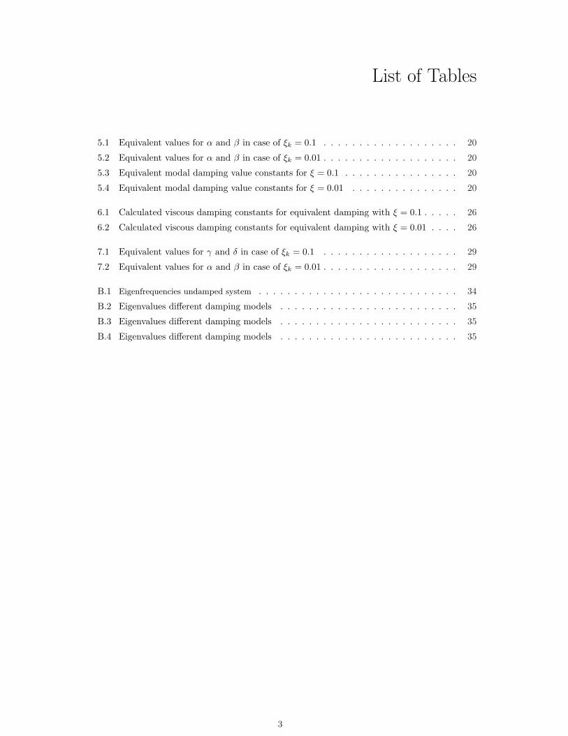
List of Tables

5.1 Equivalent values for α and β in case of ξk = 0.1 . . . . . . . . . . . . . . . . . . . 20


5.3 Equivalent modal damping value constants for ξ = 0.1 . . . . . . . . . . . . . . . . 20

5.4 Equivalent modal damping value constants for ξ = 0.01 . . . . . . . . . . . . . . . 20

6.1 Calculated viscous damping constants for equivalent damping with ξ = 0.1 . . . . . 26

6.2 Calculated viscous damping constants for equivalent damping with ξ = 0.01 . . . . 26

7.1 Equivalent values for γ and δ in case of ξk = 0.1 . . . . . . . . . . . . . . . . . . . 29


B.1 Eigenfrequencies undamped system . . . . . . . . . . . . . . . . . . . . . . . . . . . . 34

B.2 Eigenvalues different damping models . . . . . . . . . . . . . . . . . . . . . . . . . 35



3

List of Figures

1.1 Different damping models . . . . . . . . . . . . . . . . . . . . . . . . . . . . . . . . 6

2.1 Comparing generally valid equations and assuming proportional damping . . . . . 10

3.1 The modelled system . . . . . . . . . . . . . . . . . . . . . . . . . . . . . . . . . . . 13

3.2 Visualisation eigenmodes . . . . . . . . . . . . . . . . . . . . . . . . . . . . . . . . . 15

4.1 Free respons of the sixth DOF (undamped and modal damping ξ = 0.01) . . . . . 16

4.2 Energy change in case of no damping . . . . . . . . . . . . . . . . . . . . . . . . . . 17

4.3 Energy change in case of modal damping ξ = 0.01 . . . . . . . . . . . . . . . . . . 17

4.4 Bodeplot: modal damping ξ = 0.01 versus undamped . . . . . . . . . . . . . . . . . 18

5.1 Free response (Modal damping ξ = 0.01 and equivalent Rayleigh damping) . . . . . 21

5.2 Solutions for α and β for equivalent damping . . . . . . . . . . . . . . . . . . . . . 21

5.3 Equivalent modal damping factors as a function of α and β (ξ = 0.01) . . . . . . . 22

5.4 Equivalent ξ1Rto ξ6R

as a function of the eigenfrequenties (α = 0.0803 and β = 0.0705) 22

5.5 Bodeplot for modal damping (ξ = 0.01) and equivalent Rayleigh damping . . . . . 23

6.1 Energy change for interconnected DOF, equivalent with modal damping ξk = 0.01 24

6.2 Example of the FRF when a strong viscous damper has been placed between thethird and fourth DOF. . . . . . . . . . . . . . . . . . . . . . . . . . . . . . . . . . . 25

6.3 Free response when a viscous damper has been placed between the third and fourthDOF (ξk = 0.01) . . . . . . . . . . . . . . . . . . . . . . . . . . . . . . . . . . . . . 27

6.4 FRF when a viscous damper has been placed between the third and fourth DOF(ξk = 0.01) . . . . . . . . . . . . . . . . . . . . . . . . . . . . . . . . . . . . . . . . 28

7.1 FRF of structural damping compared to the FRF of modal damping ξ = 0.01 (δ = 0) 30

7.2 Difference between the FRF in case of modal damping (ξk = 0.1) structural damping(γ = 0) . . . . . . . . . . . . . . . . . . . . . . . . . . . . . . . . . . . . . . . . . . . 31

C.1 Calculation of the (6,6)-term of the frequency response matrix with first orderformulation and equation (2.14) . . . . . . . . . . . . . . . . . . . . . . . . . . . . . 36

C.2 Free respons of mass six (undamped and modal damping ξ = 0.1) . . . . . . . . . . 37

C.3 Bodeplot: modal damping ξ = 0.1 versus undamped . . . . . . . . . . . . . . . . . 37

C.4 Energy change in case of modal damping ξ = 0.1 . . . . . . . . . . . . . . . . . . . 38

C.5 Free response (Modal damping ξ = 0.1 and equivalent Rayleigh damping) . . . . . 38

C.6 Free response (α 6= 0 and beta 6= 0 ) . . . . . . . . . . . . . . . . . . . . . . . . . . 39

C.7 Equivalent modal damping factors as a function of α and β (ξ = 0.1) . . . . . . . . 39

C.8 Bodeplot for modal damping (ξ = 0.1) and two kinds of equivalent Rayleigh damp-ing . . . . . . . . . . . . . . . . . . . . . . . . . . . . . . . . . . . . . . . . . . . . 40

C.9 Bodeplot for modal damping (ξ = 0.01) and equivalent Rayleigh damping α 6= 0 enbeta 6= 0 . . . . . . . . . . . . . . . . . . . . . . . . . . . . . . . . . . . . . . . . . . 40

4

C.10 Energy change for interconnected DOF, equivalent with modal damping ξk = 0.1 . 41

C.11 FRF when a viscous damper has been placed between the sixth DOF and the solidworld (ξk = 0.01) . . . . . . . . . . . . . . . . . . . . . . . . . . . . . . . . . . . . . 41

C.12 Free response when a viscous damper has been placed between the sixth DOF andthe solid world (ξk = 0.01) . . . . . . . . . . . . . . . . . . . . . . . . . . . . . . . . 42

C.13 Energy change for DOF connected to the solid world, equivalent with modal damp-ing ξ = 0.01 . . . . . . . . . . . . . . . . . . . . . . . . . . . . . . . . . . . . . . . . 42

C.14 Energy change for DOF connected to the solid world, equivalent with modal damp-ing ξ = 0.1 . . . . . . . . . . . . . . . . . . . . . . . . . . . . . . . . . . . . . . . . 43

C.15 FRF of structural damping compared to the FRF of modal damping ξ = 0.1 (δ = 0) 43

C.16 FRF of structural damping compared to the FRF of modal damping ξ = 0.01 (γ = 0) 44

C.17 FRF of structural damping compared to the FRF of modal damping ξ = 0.1 (γ = 0) 44

5

1Introduction

Over the years modelling the behavior of dynamic systems has become more and more important,mainly because cost savings when using models instead of numerous prototypes in early stagesof development. In these models damping must be introduced to account for energy dissipa-tion during motion. This energy dissipation may depend on velocity (general viscous damping),displacement (hysteresis damping) or a combination of both. Many different ways of modellingdamping in (linear) dynamic systems are available these days. However each model possessesdifferent properties and a thorough knowledge regarding the differences between these models isnecessary in order to correctly choose and use one or more of these models.

The main goal of this report is to elucidate the differences between several damping models. Fourtypes of models will be treated in this report. After introducing the theoretical background of thefour damping models shown in figure 1.1, in chapter 2, a reference or test system is introducedin chapter 3 which will be used in the numerical analysis of several damping models which isdiscussed in chapter 4 to 7.

Damping models

General viscous damping

Rayleigh damping

Modal / proportionaldamping

Structural / hysteresis damping

Displacement dependentVelocity dependent

Figure 1.1: Different damping models

In chapter 8 these four ways of modelling damping are compared. All comparisons will be madewith respect to two levels of modal damping introduced in chapter 4. As the main references forthis report [De Kraker and Van Campen - 01] and [De Kraker - 04] have been used. Mathematicalderivations which are presented in these references will be referred to rather than repeated in thisreport.

6

2Theoretical background of damping models

After a short introduction to undamped systems the general viscous damping model will be in-troduced. The first order formulation will be derived and explained and an introduction to theinterpretation of complex eigenmodes will be made. Next three other damping models will beintroduced. Modal and Rayleigh damping are forms of general viscous damping where structuraldamping is not related to velocity but is displacement dependent.

2.1 Undamped systems

The dynamic behavior of an undamped mechanical system consisting of n degrees of freedom(DOF) is described by the following equation of motion:

M q˜(t) + K q

˜(t) = f

˜(t) (2.1)

where M (n × n) is the mass matrix and K (n × n) is referred to as the stiffness matrix. Thematrix M is positive definite and K is (semi) positive definite [De Kraker - 04]. When calculatingthe eigenvalues (or in this case undamped eigenfrequencies ωok) and undamped eigenmodes of thisundamped system the eigenvalue problem in equation (2.2) is solved.

[−ω2okM + K

]uõk = 0 k = 1, 2, ..., n (2.2)

It becomes clear that solving the eigenvalue problem in equation (2.2) leads to n real eigenfre-quencies ωok and n eigenmodes uok of the undamped system.

2.2 General viscously damped systems

In case of damped motion the systems’ dynamics are no longer fully described by equation (2.1),but an additional damping term should be added. In case of viscous damping the damping isaccounted for by adding a velocity dependent term. However in case of structural damping,damping is accounted for by means of a complex stiffness (see §2.3.4). The equation of motionthen becomes:

M q˜(t) + B q

˜(t) + K q

˜(t) = f

˜(t) (2.3)

The corresponding eigenvalue problem is defined below.

[ω2

kM + ωkB + K]u˜k = 0 k = 1, 2, ..., n (2.4)

7

This quadratic eigenvalue problem can not be solved by conventional eigenvalue solvers. In thefollowing paragraph therefore a method called first order formulation will be introduced to convertthe quadratic eigenvalue problem in equation (2.4) to a lineair eigenvalue problem that can besolved by conventional eigenvalue solvers.

First order formulation

The first order formulation as described in [De Kraker - 04], starts by rewriting the system of nsecond order, coupled differential equations in (2.3) to a set of 2n first order, coupled differentialequations, see equations (2.5) to (2.7).

C y˜(t) + D y

˜(t) = g

˜(t) (2.5)

where:

C =[

B MM 0

]D =

[K 00 −M

](2.6)

y˜(t) =

[q˜(t)

q˜(t)

]g˜(t) =

[f˜(t)0˜

](2.7)

Usually equation (2.5) leads to both a right and a left eigenvalue problem. However, the matricesof the system that will be dealt with in this report are symmetric, which leads to identical solutionsof the left and the right eigenvalue problem. Solving only one of the eigenvalue problems thensuffices. These eigenvalue problems can be formulated as below.

[λkC + D] v˜k =[λkCT + DT

]w˜k = 0˜ (2.8)

v˜k =[

u˜k

λku˜k

]w˜k =

[x˜k

λkx˜k

]

Where λk, v˜k and w˜k are the 2n eigenvalues and eigenmodes. With respect to the eigenvectors,one should realize that only the first n terms give essential information about the vibration. Thelast n terms are velocity terms that are directly related to the first n terms by the correspondingeigenvalue. For more detailed information and proof of the statements above, the reader is referredto [De Kraker - 04, §1.3].

Normalization of the (complex) eigenmodes is accomplished by dividing each of the componentsof the eigenmode by the term of the first n terms of the eigenmode with the largest modulus. Asa result one of the first n components will always be equal to 1.

For the (p, q)-term of the frequency response matrix H(ω) that relates the n physical coordinatesq˜

to the excitations f˜

we can now write:

Hp,q(ω) =2n∑

k=1

Ak(p, q)(jω − λk)

(2.9)

where:

Ak =u˜ku˜

Tk

c∗(2.10)

This relation is derived in appendix A.1. Relation (2.9) is valid for general viscously dampedsystems. This equation will be used to calculate frequency response matrices throughout thisreport. Still, in some cases, simplifications can be made to this equation. They will be introducedin §2.3.

8

2.2.1 Interpretation of complex eigenvalues and eigenmodes

The eigenvalue problem defined in equation (2.8) generally leads to 2n complex eigenvalues andeigenmodes. The imginary and real parts of the eigenvalues (λk) each have a physical meaning.The arbitrary eigenvalue λk is defined as follows:

λk = µk + jωk (2.11)

The real part of the eigenvalue (µk) now accounts for the rate of convergence to zero (µk < 0)when the system is freely vibrating with damped frequency ωk

[radsec

]using eigenmode uk as initial

conditions.

Complex eigenmodes will lead to asynchronic movement of the different DOF. This means that notall DOF pass though their equilibrium point at the same time as is the case when the eigenmodesare real.

2.2.2 Dashpots

When a physical dashpot is placed between two DOF or one DOF and the solid world this willlead to general viscous damping.

In case of a linear viscous dashpot with damping coefficient c[

Nsm

]the element damping matrix

becomes:

[fi

fi+1

]=

[c −c−c c

] [qi

qi+1

](2.12)

A remark is in order here. A higher value of c will damp out the vibration between the twoconnected DOF earlier. But the opposite may be true for the vibration of the total structure, ifthe dashpot more or less starts to behave as a rigid link.

2.3 Three other methods of modelling damping in lineardynamic systems

First the terms weakly and proportionally damped will be defined. Further on in this paragrapha short introduction with respect to different ways of modelling damping in linear dynamic sys-tems will be given. First general viscous damping is further introduced. Then modal dampingand Rayleigh damping are described. Finally structural damping will be introduced and somesimplifications are made to this particular model to make it easier to handle.

2.3.1 Weakly and proportionally damped systems

Under certain conditions equation (2.9) can be simplified, see also chapter 4. In view of thesesimplifications the terms proportional damping and weak damping should be well defined.

A thorough definition of these terms is given in [De Kraker and Van Campen - 01, p.228-240]. Inthis report weak damping will simply be defined as damping where the damped eigenmodes differlittle from the eigenmodes of the undamped system u˜k ≈ uõk. Proportional damping will bedefined as a system where UT B U results in a diagonal matrix leading to uncoupled equations ofmotion. Please note that these definitions are not equivalent, as is illustrated by figure 2.1 wherethe frequency response matrix has been calculated using (2.9) and using the simplified formulationof equation (2.14) assuming proportional damping (not weak damping!), which will be introduced

9

in §2.3.2. All modes of the system are over damped and thus not weakly damped. UT B U ,however, still results in a diagonal matrix and so the results of both equations are identical.

0 0.1 0.2 0.3 0.4 0.5 0.6 0.710

−2

100

102

Frequency [Hz]

|H(6

,6)|

[m/N

]

Modulus of H(6,6)

Equation 2.14, modal or proportional dampingEquation 2.9, general viscous damping

0 0.1 0.2 0.3 0.4 0.5 0.6 0.7 0.8−150

−100

−50

0

Frequency [Hz]

Ang

le H

(6,6

) [o ]

Phase H(6,6)


Figure 2.1: Compared calculations performed with generally valid equations and simplified equationsassuming proportional damping (modal damping ξk = 1.2).

2.3.2 Modal damping

When applying modal damping or proportional damping, a dimensionless damping factor ξk isdefined for each mode uok. A particular motion is thus damped, depending on the relative presenceof each of the systems’ modes (see chapter 3). A diagonal dimensionless damping matrix Ξ is thendefined, with diagonal elements ξk, which satisfies 2Ξ Ω = U0

T B U0. The eigenmodes in this caseare equal to the eigenmodes uõk of the undamped system so I = UT

0 M U0 and Ω2 = UT0 K U0.

Using the definition above a direct relation between the damping matrix BM and the modaldamping matrix Ξ can be formulated:

BM = 2U−T Ξ ΩU−1 (2.13)

This equation is valid for proportionally damped systems and is only approximately valid forweakly damped systems. In this report two levels of modal damping, ξk = 0.1 and ξk = 0.01 areused as reference levels of damping for the three other damping models.

Furthermore a simplification with respect to equation (2.9) can be made in case of modal damping.Assuming proportional damping the (p, q)-term of the frequency response matrix can be definedas:

Hp,q(ω) =n∑

k=1

uok˜

uok˜

T (p, q)

mk(ω2ok − ω2 + 2jξkωokω)

(2.14)

This equation is derived in [De Kraker - 04, §1.3]. A figure showing the similarity between equation(2.14) and (2.9) is included in appendix C.1 (figure C.1). Note that modal damping or proportionaldamping is a special form of general viscous damping.

10

2.3.3 Rayleigh damping

Sometimes damping is assumed to be proportional to the mass and stiffness matrix. This is calledRayleigh damping. The damping matrix can then be formulated as:

BRαβ= α M + β K (2.15)

Because this model only possesses two variables it’s of little use when tuning of multiple modesis required. A direct relation between modal and Rayleigh damping can easily be derived whencombining equation (2.13), (2.15) and the basic relations defined in the first alinea of §2.3.2.

ΞRαβ=

12UT [αM + βK] U Ω−1 (2.16)

ΞRαβ=

12αI Ω−1 +

12β Ω (2.17)

Note that Rayleigh damping is a special form of modal damping.

2.3.4 Structural damping or hysteresis damping

Structural damping is used in situations where energy dissipation depends on displacement andnot on velocity. In this case terms as introduced in equation (2.3) will thus have no effect. Inthe case of structural damping or hysteresis damping this is accomplished by introducing complexstiffness. The equation of motion and the eigenvalue problem below describe this model.

M q(t) +[K + jHs

]q(t) = f

˜ejωt (2.18)

[λ2

kM +(K + jHs

)]u˜k = 0˜ (2.19)

One of the advantages of equation (2.19) is that the eigenvalue is of the form of equation (2.2) andcan thus be solved by conventional eigenvalue solvers. However, calculation of the matrix Hs toobtain a certain level of damping will be very difficult. This problem originates in te fact that theeigenmodes uk

ãre necessary to calculate Hs and that Hs is needed to calculate the eigenmodes

on their turn... The structural damping matrix Hs is therefore defined as:

Hs = γM + δK (2.20)

In this case the corresponding eigenvalue problem becomes:

[λ2 + jγ

1 + jδM + K

]u˜ = 0˜ (2.21)

It’s now possible to define the solutions of this eigenvalue problem as shown below. Furthermorea so called structural loss factor ηk is defined, which can be expressed in the parameters γ, δ andωok.

u˜k = uõk λk = jωok

√1 + jηk (2.22)

ηk = δ +γ

ω2ok

(2.23)

11

These solutions are only valid for proportionally structurally damped systems. For an elaboratederivation of the equations and solutions in this paragraph, the reader is referred to [De Kraker - 04,§1.4].

Because the only damping parameters used in equation (2.20) to (2.23) are γ, δ and known systemparameters this formulation makes it possible to compare structural damping to modal damping.The equation used to calculate frequency response matrix can again be simplified and is definedas in (2.24). Again the reader is referred to [De Kraker - 04, §1.4] for more information.

H(ω) =n∑

k=1

uõku˜Tok

mk [ω2ok − ω2 + jω2

okηk](2.24)

Because of the non-physical character of this structural damping model it is only applicable in thefrequency domain. In order to compare the motion of a system to the motion obtained when modaldamping is applied, frequent Fourier and inverse Fourier transformation is necessary. Because ofsignificant disadvantages (signal leakage and aliasing), a more elegant methode is chosen whichwill be described in chapter 7. One of the difficulties of structural damping modal is that it resultsin non-causal behavior in the time domain. This means that the system responds to forces beforethey are actually applied.

12

3The reference system

3.1 General

In this report the different damping models are explored and compared by means of a simplesystem consisting of six masses of m = 0.5 kg each which are connected by six linear springs withspring stiffness k = 2 N

m , see figure 3.1.

M = 0.5 [kg]1 M = 0.5 [kg]2M = 0.5 [kg]6

K = 2 [N/m]1 K = 2 [N/m]2 k = 2 [N/m]6

x ,f1 1 x ,f2 2x ,f6 6

Figure 3.1: The modelled system

The mass and stiffness matrix are easily determined for this undamped system and result in thefollowing equation of motion:

Mq˜(t) + Kq

˜(t) = f

˜(t) (3.1)

Pleas note that on the remaining pages of this report all figures and FRF’s presentedresemble the movement or direct transfer function1 of the sixth DOF.

3.2 Initial displacement

In this report a force will only be applied to the sixth DOF. A static initial displacement of 0.1 mof this DOF is assumed for investigation of the free vibration. To calculate the force necessary toaccomplish a displacement of 0.1 m for the sixth DOF and to calculate the displacements of allother mass Finite Element Methode (FEM) will be used. A column q

˜containing all displacements

and a column f˜

containing all external forces acting on the system are introduced. After evaluatingforce balance in the system it follows that:

Kq˜

= f˜

(3.2)

1The direct transfer function is the response of a DOF related to a force applied on this DOF.

13

After realizing that all terms of f˜

except f˜

6 are zero and q˜

f = [q1 q2 q3 q4 q5]T is unknown while

q˜

g = q˜6 = 0.1 m the system can be partitioned as below.

Kff | Kgf

− + −Kfg | Kgg

q˜

f

−0.1

=

0−f˜

g

(3.3)

fg

˜= Kgg q

˜g + Kfg q

˜f (3.4)

The force needed to realize the prescribed displacement turns out to be fg = f6 = 0.033 N andq˜

g = [q1 q2 q3 q4 q5]T = [0.017 0.033 0.05 0.067 0.083]T .

3.3 Undamped eigenmode and eigenfrequencies

With both the stiffness matrix and mass matrix know, the undamped eigenvalues and undampedeigenmodes of this system can be calculated as defined in §2.1. The results are shown below.

f1

f2

f3

f4

f5

f6

=

0.48211.41842.27232.99403.54183.8838

rad

sec=

0.07670.22570.36160.47650.56370.6181

Hz (3.5)

u˜T1

u˜T2

u˜T3

u˜T4

u˜T5

u˜T6

T

=

−0.1877 0.5202 −0.7335 0.7787 0.6456 −0.3646−0.3646 0.7787 −0.5202 −0.1877 −0.7335 0.6456−0.5202 0.6456 0.3646 −0.7335 0.1877 −0.7787−0.6456 0.1877 0.7787 0.3646 0.5202 0.7335−0.7335 −0.3646 0.1877 0.6456 −0.7787 −0.5202−0.7787 −0.7335 −0.6456 −0.5202 0.3646 0.1877

(3.6)

The eigenmodes has been normalized with respect to M so that UT M U = I. Each term in eacheigenmode describes the amplitude of DOF concerned. When this is visualized as in figure 3.2it is clear that the first mode looks much like the initial static displacement found in §3.2. Thisstatement can also be formulated in a more mathematical way if an arbitrary displacement isdefined as a weighted sum of the eigenmodes.

q˜

=n∑

k=1

aku˜k (3.7)

In this case we find that a1 = 0.11 while the sum of all other weight factors is less than 0.02. Itcan now be formally stated that the first mode is dominantly present in the chosen initial staticdisplacementfield. This knowledge will be used in chapter 7, where hysteresis damping is discussed.The effects of the great resemblance between the first mode and the initial static displacementfield are visible in all bodeplots in this report.

14

1

2

3

4

5

6

Figure 3.2: Visualisation of the eigenmodes

3.4 Equivalent damping

The term equivalent damping will be frequently used when comparing different models. Thismeans that 90 percent of the systems’ total energy should have been dissipated within a giventime span. Two levels of modal damping will be used as reference. The time at which 90 percentof the total energy has been dissipated (t = τ) can be formulated as the time when:

12 q˜(τ)M q

˜(τ)T + 1

2 q˜(τ)K q

˜(τ)T

12 q˜(0)M q

˜(0)T + 1

2 q˜(0) K q

˜(0)T

= 0.1 (3.8)

where the static displacement field of section 3.2 is taken as q˜(0) and q

˜(0) = 0. Because q

˜(0)

resembles the first mode very much, not only will both compared models have dissipated an equalamount of energy at t = τ but the first peaks in the bodeplot will also look very similar. Thisknowledge is used in chapter 7 for calculation equivalent damping in case of structural dampingin the frequency domain. It should be noted that any equivalent damping constant found in thisreport is only valid for the given initial conditions q

˜(0) and q

˜(0) = 0.

15

4Modal damping

As stated in §2.3.2 modal damping is a damping model where each mode is damped by a di-mensionless constant ξk. Two levels of modal damping (ξk = 0.01) and (ξk = 0.1) are used as areference for other ways of modelling damping in the next three chapters. In this chapter modaldamping will be introduced.

4.1 Free vibration

Because both damping factors result in an under damped system (ξk < 1), the systems’ movementwhen released from the initial displacement introduced in §3.2, is expected to be a vibration withdecreasing amplitude. This is shown for ξk = 0.01 in figure 4.1. A similar figure for ξk = 0.1 canbe found in appendix C.2 (figure C.2). The ∗-sign indicates the point at which 90 percent of thetotal energy has been dissipated (t = τ). Calculations show that 90 percent of the total energyhas been dissipated after τξ0.1 = 22.94 s in case of ξk = 0.1 and after τξ0.01 = 224.75 s in case ofξk = 0.01.

0 50 100 150 200 250−0.1

−0.08

−0.06

−0.04

−0.02

0

0.02

0.04

0.06

0.08

0.1

Time [s]

Dis

plac

emen

t m6 [m

]

Modal or proportional damping ξ = 0.01Undamped

Figure 4.1: Free respons of mass six (undamped and modal damping ξ = 0.01)

The figures below illustrate the change of energy in both the undamped and modally damped(ξk = 0.01) case. Any change in the amplitude of the vibration of the sixth DOF in cases of the

16

undamped system, in figure 4.1, originates in energy transfer beween different masses. In figure4.3 a significant decrease in energy is seen as a result of modal damping. A similar figure forξk = 0.1 is presented in appendix C.2 (figure C.4). This energy decrease has been used and willbe used to formulate a specific time at which the specified amplitude decrease (90 percent) hasbeen accomplished (τξ0.1 and τξ0.01).

0 5 10 15 20 25 30 35 40 45 500

0.2

0.4

0.6

0.8

1

1.2

1.4

1.6

1.8x 10

−3

Time [sec]

Ene

rgy

[J]

Potential energy (undamped)Kinetic energy (undamped)Total energy (undamped)

Figure 4.2: Energy change in case of no damping

0 50 100 150 200 2500

0.2

0.4

0.6

0.8

1

1.2

1.4

1.6

1.8x 10

−3

Time [sec]

Ene

rgy

[J]

Potential energy (ξ = 0.01)Kinetic energy (ξ = 0.01)Total energy (ξ = 0.01)

Figure 4.3: Energy change in case of modal damping ξ = 0.01

17

4.2 Forced vibration

The eigenvalues in case of modal damping with damping level ξk = 0.1 and ξk = 0.01 have beenincluded in appendix B. In the direct FRF of the sixth DOF the resonance peaks also appear atalmost the same frequency as in the undamped case. These resonance and antiresonance peaksare, however, less high and less steep as is to be expected in a damped system. The FRF formodal damping in case of ξk = 0.1 can be found in appendix C.2 (figure C.3).

0 0.1 0.2 0.3 0.4 0.5 0.6 0.710

−2

100

102

Frequency [Hz]

|H(6

,6)|

[m/N

]

Modulus of H(6,6)


0 0.1 0.2 0.3 0.4 0.5 0.6 0.7 0.8−200

−100

0

100

200

Frequency [Hz]

Ang

le H

(6,6

) [o ]

Phase H(6,6)


Figure 4.4: Bodeplot: modal damping ξ = 0.01 versus undamped

18

5Rayleigh damping

When the damping matrix is assumed to be proportional to the mass and stiffness matrix, this iscalled Rayleigh damping. This damping model has been introduced in §2.3.3. For the calculationof the damping matrix, equation (2.15) has been formulated. This equation is repeated here forthe readers convenience.

BRαβ= α M + β K (5.1)

This chapter will focus on finding values for α, β that damp the system in such a way that 90percent of all energy will have dissipated after either τξ0.1 = 22.94 s or τξ0.01 = 224.75 s. Pleasenote that these are the reference times already found for modal damping in §4.1.

First the cases where α = 0, β > 0 and α > 0, β = 0 are dealt with. Then combinations of α andβ will be looked at in more detail1. Because Rayleigh damping is a special form of modal dampinga closer look will also be taken at the equivalent damping factors resulting from equation (2.17),which is also repeated here:

ΞRαβ=

12αI Ω−1 +

12β Ω (5.2)

Finally the FRF’s for different forms of Rayleigh damping will be presented and compared withthose resulting from modal damping. The eigenvalues and eigenmodes calculated in chapter 3remain almost the same (for the evaluated cases of equivalent damping) and can be found inappendix B.

5.1 Damping only proportional to the mass matrix (α > 0,β = 0) or stiffness matrix (α = 0, β > 0)

If damping is only proportional to the mass matrix equation (5.1) and (5.2) simplify becausethe last terms of these equations become zero. Calculation of equivalent values for α, so thatthe system dissipates 90 percent of it’s energy in respectively τξ0.1 = 22.94 s or τξ0.01 = 224.75 s,seconds have been performed using matlab.

A similar calculation was performed in case of α = 0, β > 0. The results for equivalent dampingare presented below. The factor 10 which is present in the two considered modal damping levelsξk = 0.01 and ξk = 0.1 dos not stay exactly 10 when comparing the equivalent damping values forα and β.

1Please note that all equivalent constants presented are only equivalent for the free vibration based on the initialconditions qe(0) as defined in §3.2 and qe(0) = 0.

19

ξk = 0.1 β = 0 β =α = 0 X 0.4145α = 0.1026 figure 5.2

Table 5.1: Equivalent values for α and β in case of ξk = 0.1

ξk = 0.01 β = 0 β =α = 0 X 0.0415α = 0.0103 figure 5.2


Using equation (5.2) it is now possible to calculate the modal damping factors ξkRfor the different

values of α and β that are presented in table 5.1 and 5.2. The eigenvalues for the cases presentedin 5.1 and 5.2 can be found in appendix B.

α = 0.1026 β = 0 α = 0 β = 0.4145ξ1R 0.1064 0.0999ξ2R 0.0362 0.2940ξ3R 0.0226 0.4709ξ4R 0.0171 0.6205ξ5R 0.0145 0.7340ξ6R 0.0132 0.8049

Table 5.3: Equivalent modal damping value constants for ξ = 0.1

α = 0.0103 β = 0 α = 0 β = 0.0415ξ1R

0.0106 0.0100ξ2R

0.0036 0.0294ξ3R

0.0023 0.0471ξ4R

0.0017 0.0620ξ5R

0.0145 0.0734ξ6R

0.0014 0.0805

Table 5.4: Equivalent modal damping value constants for ξ = 0.01

Tables 5.3 and 5.4 show that the equivalent modal damping constant of the first mode is almostequal to respectively 0.1 and 0.01 while all other equivalent damping constants are significantlylarger or smaller. This is a result of the resemblance between the initial static displacement field(on which all values are based) and the first mode (see §3.3). The damping factor ξ1 of thefirst mode will therefore dominate the free vibration compared to the dampening factors of theother modes. When calculating damping factors that result in the same free vibration as modaldamping2 (ξk = 0.01 or ξk = 0.01) ξ1R

will thus bo close to respectively 0.01 or 0.1. In case ofα = 0 the tables above show that the higher modes are damped stronger than the first modewhile the opposite is true when β = 0. This also follows directly from equation (5.2). The nextparagraph shows how the different equivalent modal damping factors behave when α and β vary.

Figure 5.1 gives a graphical representation of the movement of the sixth mass when two kinds ofRayleigh damping are applied. The free responses are not exactly the same, but the indicated

2It should again be noted that all equivalent constants presented are only equivalent for the free vibration basedon the initial conditions qe(0) as defined in §3.2 and qe(0) = 0.

20

times when 90 percent of the total energy has been dissipated, are identical. A similar figure incase of ξk = 0.1 can be found in appendix C.3 (figure C.5).

0 50 100 150 200 250−0.1

−0.08

−0.06

−0.04

−0.02

0

0.02

0.04

0.06

0.08

0.1

Time [s]

Dis

plac

emen

t m6 [m

]Modal or proportional damping ξ = 0.01Rayleigh damping α = 0.0103, β = 0Rayleigh damping α = 0, β = 0.0415

Figure 5.1: Free response (modal damping ξ = 0.01 and equivalent Rayleigh damping)

5.2 Damping proportional to both the mass matrix and thestiffness matrix (α > 0, β > 0)

In the preceding paragraph a number of calculations were performed to calculate equivalent valuesfor α and β for equivalent damping with modal damping with ξk = 0.1 and ξk = 0.01. Naturally,a range of solutions exists when both α > 0 and β > 0. In figure 5.2 these solutions are shown.In appendix C.3 (figure C.6) a graph showing the motion of the sixth mass when damped by thiskind of Rayleigh damping has been included to verify these results.

0 0.02 0.04 0.06 0.08 0.1 0.120

0.05

0.1

0.15

0.2

0.25

0.3

0.35

0.4

0.45

α [−]

β [−

]

Modal or proportional damping ξ = 0.1Modal or proportional damping ξ = 0.01

Figure 5.2: Solutions for α and β for equivalent damping with modal damping (ξ = 0.1 and ξ = 0.01)

21

An infinite number of combinations of α and β are thus possible, all producing the desired result.This should result in an infinite number of corresponding sets of equivalent modal damping factors.Figure3 5.3 shows how the different equivalent modal damping factors change for different combi-nations of α and β. As already noted in the preceding paragraph the effect of stronger dampingof the higher modes when α = 0, β > 0 and weaker damping of these modes when α > 0, β = 0can also be observed here. Another effect is shown by plotting the different equivalent modaldamping factors with respect to the eigenfrequencies corresponding to the different eigenmodes ofthe system for combination α = 0.0803 and β0.0705. A clear minimum is observed in figure 5.4.

0 0.002 0.004 0.006 0.008 0.01 0.0120

0.02

0.04

0.06

0.08

0.1ξ(α, β) (equivalent with ξ = 0.01)

α [−]

ξ [−

]

ξ1

ξ2

ξ3

ξ4

ξ5

ξ6

0 0.02 0.04 0.06 0.08 0.1 0.120

0.1

0.2

0.3

0.4

0.5α(β) (equivalent with ξ = 0.1)

α [−]

β [−

]

Figure 5.3: Equivalent modal damping factors as a function of α and β (equivalent for modal damping(ξ = 0.01))

0 0.1 0.2 0.3 0.4 0.5 0.6 0.70.07

0.08

0.09

0.1

0.11

0.12

0.13

0.14

0.15

0.16

Eigenfrequency (ωok

/2π) [Hz]

ξ [−

]

Figure 5.4: Equivalent ξ1R to ξ6R as a function of the eigenfrequenties (α = 0.0803 and β = 0.0705)

3A similar figure for the situation where ξk = 0.1 is included in appendix C.3 (figure C.7).

22

5.3 Forced vibration

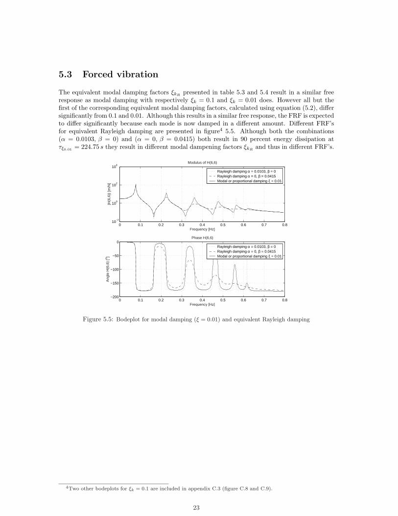
The equivalent modal damping factors ξkRpresented in table 5.3 and 5.4 result in a similar free

response as modal damping with respectively ξk = 0.1 and ξk = 0.01 does. However all but thefirst of the corresponding equivalent modal damping factors, calculated using equation (5.2), differsignificantly from 0.1 and 0.01. Although this results in a similar free response, the FRF is expectedto differ significantly because each mode is now damped in a different amount. Different FRF’sfor equivalent Rayleigh damping are presented in figure4 5.5. Although both the combinations(α = 0.0103, β = 0) and (α = 0, β = 0.0415) both result in 90 percent energy dissipation atτξ0.01 = 224.75 s they result in different modal dampening factors ξkR

and thus in different FRF’s.

0 0.1 0.2 0.3 0.4 0.5 0.6 0.7 0.810

−2

100

102

104

Frequency [Hz]

|H(6

,6)|

[m/N

]

Modulus of H(6,6)

Rayleigh damping α = 0.0103, β = 0Rayleigh damping α = 0, β = 0.0415Modal or proportional damping ξ = 0.01

0 0.1 0.2 0.3 0.4 0.5 0.6 0.7 0.8−200

−150

−100

−50

0

Frequency [Hz]

Ang

le H

(6,6

) [o ]

Phase H(6,6)

Rayleigh damping α = 0.0103, β = 0Rayleigh damping α = 0, β = 0.0415Modal or proportional damping ξ = 0.01

Figure 5.5: Bodeplot for modal damping (ξ = 0.01) and equivalent Rayleigh damping

4Two other bodeplots for ξk = 0.1 are included in appendix C.3 (figure C.8 and C.9).

23

6Viscous damping

General viscous damping is obtained when using dashpot elements. As described in §2.2.2 thedamping matrix is easily constructed, but for some system configurations it appeares to be im-possible to place a damper strong enough to dissipate enough energy within the specified timespans.

The following example illustrates this. Viscous dampers are placed between different two DOF (notthe solid world). It’s now possible to compute the total energy of the system at τξ0.01 = 224.75 sas a function of the viscous damping constant c. Figure 6.1 it shows that for four out of the fivepossible locations, it is possible to define a viscous damping constant that leads to a 90 percentdecrease in energy at time τξ0.01 = 224.75 s. However, if the damper is placed between the fifthand sixth DOF, the total energy reaches a minimum of about 32 percent around c = 4Ns

m and thenstarts to increase, because the effect of linking the two mass starts to dominate the dissipationcapacity of the damper. Increasing the damping constant wil now only lead to more synchronicmovement of the fifth and sixth DOF. An extreme example of this effect is given in §6.2. Moreenergy graphs are included in appendix C.4 (figure C.10, C.13 and C.14). These support theequivalent viscous damping constants presented in this chapter but are excluded from this text toincrease readability of this report.

0 1 2 3 4 5 60

0.1

0.2

0.3

0.4

0.5

0.6

0.7

0.8

0.9

1

c [Ns/m]

Eto

tal /

E0

[−]

Dashpot interconnecting m1 and m

2 (eq. ξ = 0.01)


3 (eq. ξ = 0.01)


4 (eq. ξ = 0.01)


5 (eq. ξ = 0.01)


6 (eq. ξ = 0.01)

Figure 6.1: Energy change at τξ0.01 = 224.75 s (equivalent with modal damping ξk = 0.01) as afunction of the viscous damping constant c for interconnected DOF.

24

6.1 Eigenvalues and eigenvectors

In case of modal and Rayleigh damping it has been observed that the eigenvalues and eigenvectorsdid not significantly change with respect to the undamped eigenvectors and eigenvalues (for eigen-values see appendix B). Moreover all the eigenvectors were found to be the real eigenvectors ofthe undamped system, which means that all DOF pass through zero at the same time. In generalviscously damped systems the eigenvectors will, however, be complex, and the different DOF willnot pass through zero at the same time. The interpretation of the eigenvectors is much moredifficult in these cases, because we now have include the phase difference as well as the amplitudein the interpretation.

6.2 An extreme example

An (almost) infinitely strong damper placed between the third and fourth DOF gives a clearillustration of the effect described in the introduction of this chapter. In this case the FRF isgiven by figure 6.2 and only five resonance peaks are found instead of the former six.

0 0.1 0.2 0.3 0.4 0.5 0.6 0.710

−2

100

102

Frequency [Hz]

|H(6

,6)|

[m/N

]

Modulus of H(6,6)


4 (semi rigid link)

Modal or proportional damping ξ = 0.01

0 0.1 0.2 0.3 0.4 0.5 0.6 0.7 0.8−200

−150

−100

−50

0

Frequency [Hz]

Ang

le H

(6,6

) [o ]

Phase H(6,6)


4 (semi rigid link)


Figure 6.2: Example of the FRF when a strong viscous damper has been placed between the thirdand fourth DOF.

The complex eigenvalues offer an explanation in this case. Close examination of the eigenvaluesshows that the complex part (responsible for the vibration frequency) of λ7,8 and λ9,10 are almostthe same. In the FRF they will show up as one peak. One should however realize that no matterhow few peak show up in the FRF there will always be 2n = 12 distinct complex conjugatedeigenvalues and eigenmodes .

25

λ1,2 = −0.0048± 0.4828i (6.1)λ3,4 = −0.0596± 1.4394i (6.2)λ5,6 = −0.0358± 2.2990i (6.3)λ7,8 = −0.9456± 3.2767i (6.4)

λ9,10 = −0.1873± 3.2909i (6.5)λ11,12 = −0.0127± 3.5599i (6.6)

6.3 Equivalent values for viscous damping

Equivalent dashpot damping, with respect to modal damping levels ξk = 0.01 and ξk = 0.1 fromchapter 4 can now be further investigated. The energy graphs presented at the beginning of thischapter show that only a limited number of optional locations exist to place a viscous damper. Intable 6.1 and 6.2 the result of the performed calculations are presented1. The eigenvalues for anumber of situations presented in table 6.1 and 6.2 can be found in appendix B.

Table 6.1: Calculated viscous damping constants for equivalent damping with ξ = 0.1

Location viscous damper Calculated viscous damping constants [Ns/m]Between DOF 1 and 2 ImpossibleBetween DOF 2 and 3 ImpossibleBetween DOF 3 and 4 ImpossibleBetween DOF 4 and 5 ImpossibleBetween DOF 5 and 6 ImpossibleBetween DOF 1 and solid world ImpossibleBetween DOF 2 and solid world 0.7469Between DOF 3 and solid world 0.3795Between DOF 4 and solid world 0.3816Between DOF 5 and solid world 0.2621Between DOF 6 and solid world 0.1741

Table 6.2: Calculated viscous damping constants for equivalent damping with ξ = 0.01

Location viscous damper Calculated viscous damping constants [Ns/m]Between DOF 1 and 2 0.3131Between DOF 2 and 3 0.4376Between DOF 3 and 4 0.6229Between DOF 4 and 5 1.3732Between DOF 5 and 6 ImpossibleBetween DOF 1 and solid world 0.2740Between DOF 2 and solid world 0.0746Between DOF 3 and solid world 0.0381Between DOF 4 and solid world 0.0363Between DOF 5 and solid world 0.0262Between DOF 6 and solid world 0.0177

1The values correspond to the previously defined initial excitation an are only valid for this specific initialconditions qe(0) (static displacement field) and qe(0) = 0.

26

Checking the results that are presented in the tables above, one should realize that ξk is in theorder of c

2√

km= c

2 , which corresponds to the values that are presented here. Another importantconclusion that should be drawn from table 6.1 and 6.2, is that the equivalent damping constantincreases when we interconnect two DOF further from the solid world and that the calculated valuesdecrease when we connect a DOF further from the solid world to the solid world. Dampers betweentwo DOF further in the chain cannot influence the motion of the system as good as dampers placedcloser to the solid world. This is why higher viscous damper constants are necessary to accomplishequivalent damping. An example of the free vibration2 of the sixth DOF when a viscous dashpotis placed between the third and fourth DOF is given in figure 6.3 (third case in table 6.2).

0 50 100 150 200 250−0.1

−0.08

−0.06

−0.04

−0.02

0

0.02

0.04

0.06

0.08

0.1

Time [sec]

Dis

plac

emen

t m6 [m

]

Dashpot between m3 and m

4 (eq. ξ = 0.01)


Figure 6.3: Free response when a viscous damper has been placed between the third and fourthDOF (equivalent with modal damping ξk = 0.01)

.

6.4 The Frequency Response Function

The FRF in figure 6.4 refers to the case where a dashpot with c = 0.6229 Nsm (equivalent damping

ξk = 0.01) has been placed between the third and fourth DOF. Another FRF for one of the casespresented in table 6.1 and 6.2 is presented in appendix C.4 (figure C.11).

2A similar graph for equivalent damping in case of ξk = 0.1 is included in appendix C.4 (figure C.12)

27

0 0.1 0.2 0.3 0.4 0.5 0.6 0.710

−2

100

102

Frequency [Hz]

|H(6

,6)|

[m/N

]

Modulus of H(6,6)


4 (eq. ξ = 0.01)


0 0.1 0.2 0.3 0.4 0.5 0.6 0.7 0.8−200

−150

−100

−50

0

Frequency [Hz]

Ang

le H

(6,6

) [o ]

Phase H(6,6)


4 (eq. ξ = 0.01)


Figure 6.4: FRF when a viscous damper has been placed between the third and fourth DOF(equivalent with modal damping ξk = 0.01).

28

7Structural damping or hysteresis damping

As already stated in §2.3.4, in case of structural damping, energy dissipation is not modelled by adamping matrix, but by means of complex stiffness. The energy dissipation is no longer dependenton velocity. Complex stiffness is no property that can be derived using physical laws. It can onlybe applied in the frequency domain, because it leads to non causal behavior in the time domain,which means that the system responds to forces before they are actually applied. This is simplystated here as a property of structural damping. In this report no further attention will be givento the concept of non-causal behavior.

7.1 Fitting first mode resonance peak FRF

Because structural damping is applied in the frequency domain, frequent Fourier and inverseFourier transformation would be necessary to find the appropriate hysteretic damping constants(γ and δ, see §2.3.4) for equivalent damping. In case of the particular system and the free vibrationintroduced in chapter 3, it has been shown that the first mode shows a close resemblance to theinitial static displacement field. In the former chapters it has been observed that equivalentdamping more or less leads to equality of the first resonance peak (see FRF’s plotted). Thisknowledge can now be used to find equivalent damping factors in case of structural damping.Instead of calculating the total energy as a function of time, the peak of the FRF in case ofstructural damping is fitted to the first peak of the FRF in case of modal damping. The calculatedvalues are presented in table 7.1 and 7.2.

ξk = 0.1 δ = 0 δ =γ = 0 X 0.1992γ = 0.0460 X

Table 7.1: Equivalent values for γ and δ in case of ξk = 0.1

ξk = 0.01 δ = 0 δ =γ = 0 X 0.0199γ = 0.0046 X


The factor 10 which is present in the two considered modal damping levels ξk = 0.01 and ξk =0.1 dos not stay exactly 10 when comparing the equivalent damping values for γ and δ.. Theeigenvalues in case of the situations presented in table 7.1 and 7.2 can be found in appendix B.It’s striking that the values of δ seem almost twice the values of ξk if γ = 0. This phenomenon

29

can be explained by comparing equation (2.14) and (2.24) using equation (2.23), repeated below.Note that only the Rayleigh variant of hysteresis damping is considered where Hs = γM + δK.

Hp,q(ω) =n∑

k=1

uok˜

uok˜

T (p, q)

mk(ω2ok − ω2 + 2jξkωokω)

(7.1)

H(ω) =n∑

k=1

uõku˜Tok

mk [ω2ok − ω2 + jω2

okηk](7.2)

ηk = δ +γ

ω2ok

(7.3)

If δ = 0 and γ > 0 the relation between γ and ξk follows from comparing of the last terms in thedenominator of equation (7.1) and (7.2).

δ = 0 ⇒ γ = 2ξkωωok (7.4)

This proces is repeated for the case where γ = 0 and δ > 0.

γ = 0 ⇒ δ = 2ξkω

ωok(7.5)

In case of equation (7.4) it is clear that higher modes will be less damped than lower modes (seenext paragraph). In case of equation (7.5) (γ = 0) for equivalent damping one should expect δto be equal to 2ξk when the system is vibrating in eigenmode uok with the undamped frequencyωok. This is indeed approximately the case if when the system is vibrating freely with the staticdisplacement field q

˜(0) defined in §3.2 and q

˜(0) = 0, as initial conditions. These effects also

influences the FRF’s in both cases γ = 0 and δ = 0. This will be discussed in the next paragraph.Next to that the first peaks show great resemblance due to the applied fitting procedure.

7.2 FRF in case of structural damping

When looking at the FRF in case of δ = 0 and γ = 0.0046 (figure 7.1)1 it’s observed that thehigher modes are clearly less damped than the lower modes because ξk = γ

2ωωok.

0 0.1 0.2 0.3 0.4 0.5 0.6 0.710

−2

100

102

Frequency [Hz]

|H(6

,6)|

[m/N

]

Modulus of H(6,6)

Modal or proportional damping ξ = 0.01Structural or hysteresis damping δ = 0

0 0.1 0.2 0.3 0.4 0.5 0.6 0.7 0.8−200

−150

−100

−50

0

Frequency [Hz]

Ang

le H

(6,6

) [o ]

Phase H(6,6)


Figure 7.1: FRF of structural damping compared to the FRF of modal damping ξ = 0.01 (fitting firstresonance peak) γ = 0.00460 en δ = 0

1A similar figure for ξk = 0.1 can be found in appendix C.5 (figure C.15)

30

If δ = 0.01992 and γ = 0 the FRF’s of modal and structural damping seem to be the same overthe whole frequency range. Equation (7.5), however, shows that this would only exactly be thecase when (ω = ωok). As shown below2 both FRF’s are not exactly the same and a clear drop inerror is observed when approaching ω = ωok.

0 0.1 0.2 0.3 0.4 0.5 0.6 0.710

−2

100

102

Frequency [Hz]

|H(6

,6)|

[m/N

]

Modulus of H(6,6)

Modal or proportional damping ξ = 0.1Structural or hysteresis damping γ = 0

0 0.1 0.2 0.3 0.4 0.5 0.6 0.7 0.810

−5

100

Frequency [Hz]

Err

or [m

/N]

Figure 7.2: Difference between the FRF in case of modal damping (ξk = 0.1) structural damping (γ = 0)

2Although modal damping with ξk = 0.01 had been used as reference throughout this report an exception hasbeen made in case of the FRF in figure 7.2 because the described effects are much better shown in case of ξk = 0.1than in case of ξk = 0.01.

31

8Conclusions

In this report four different damping models for dynamic systems have been presented. The modelscompared are general viscous damping, modal or proportional damping, Rayleigh damping andstructural or hysteresis damping. Each of the models possesses different properties and has it’sadvantages and disadvantages. The first three models are velocity dependent whereas the lattermodel is displacement dependent.

General viscous damping occurs in systems where discrete dashpots are applied. Eigenmodes willgenerally be complex, which means that not each DOF passes through it‘s zero at the same time.This makes interpretation of these complex eigenmodes more difficult than for real eigenmodes.

In case of modal damping each eigenmode is damped separately. This means that there are as manydamping coefficients as there are modes, which enables easy tuning of these coefficients with respectto measurements. The eigenmodes of modally damped systems are real (after normalization) whichmeans that all DOF pass through their zeros at the same time. Modal damping is a subclass ofgeneral viscous damping.

Rayleigh damping leads to a damping matrix proportional to the mass and stiffness matrix. Onlytwo tuning parameters are available. Consequently the damping levels of only two modes can betuned independently, which may lead to unrealistic damping levels for the other modes. Rayleighdamping is a subclass of modal damping. The eigenmodes remain real.

For systems in which displacement dependent energy dissipation takes place structural or hysteresisdamping can be applied. In this case energy dissipation is modelled by a complex stiffness. Thiskind of damping is only applied in the frequency domain because it leads to non-causal behaviorin the time domain. As may be expected, the eigenmodes in case of structural damping will becomplex.

In this report the free and forced vibrations of a specific structure have been studied for theseveral damping models. Two modal damping levels have been taken as a reference and equivalentdamping values have been obtained for the other damping models based on the free vibrationbehavior. These values are however only valid for this specific structure and the initial conditionsused. The advantages an disadvantages of the different models have been discussed using thesecalculations in combination with existing theory.

32

ADerivations

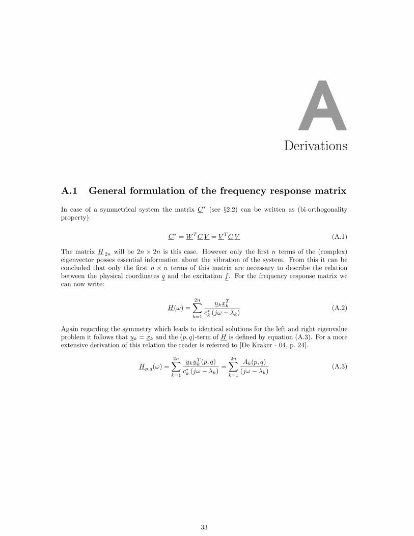
A.1 General formulation of the frequency response matrix

In case of a symmetrical system the matrix C∗ (see §2.2) can be written as (bi-orthogonalityproperty):

C∗ = WT C V = V T C V (A.1)

The matrix H 2n will be 2n × 2n is this case. However only the first n terms of the (complex)eigenvector posses essential information about the vibration of the system. From this it can beconcluded that only the first n × n terms of this matrix are necessary to describe the relationbetween the physical coordinates q

ãnd the excitation f

˜. For the frequency response matrix we

can now write:

H(ω) =2n∑

k=1

u˜kx˜Tk

c∗k (jω − λk)(A.2)

Again regarding the symmetry which leads to identical solutions for the left and right eigenvalueproblem it follows that u˜k = x˜k and the (p, q)-term of H is defined by equation (A.3). For a moreextensive derivation of this relation the reader is referred to [De Kraker - 04, p. 24].

Hp,q(ω) =2n∑

k=1

u˜ku˜Tk (p, q)

c∗k (jω − λk)=

2n∑

k=1

Ak(p, q)(jω − λk)

(A.3)

33

BEigenvalues

Table B.1: Eigenfrequencies undamped system

Eigenfrequency[

radsec

]ω1 0.4821ω2 1.4184ω3 2.2723ω4 2.9940ω5 3.5418ω6 3.8838

34

A Modal damping: ξk = 0.01

B Modal damping: ξk = 0.1

C Rayleigh damping: α = 0.0103, β = 0, equivalent with ξ = 0.01

D Rayleigh damping: α = 0.1026, β = 0, equivalent with ξ = 0.1

E Rayleigh damping: α = 0, β = 0.0415, equivalent with ξ = 0.01

F Rayleigh damping: α = 0, β = 0.4145, equivalent with ξ = 0.1

G General viscous damping: Viscous damper between m6 and world, c = 0.0177, equivalent withξk = 0.01

H General viscous damping: Viscous damper between m6 and world, c = 0.1741, equivalent withξk = 0.1

I Hysteresis damping: δ = 0, γ = 0.0046, equivalent with ξ = 0.01

J Hysteresis damping: δ = 0, γ = 0.0460, equivalent with ξ = 0.1

K Hysteresis damping: δ = 0.0199, γ = 0, equivalent with ξ = 0.01

L Hysteresis damping: δ = 0.1992, γ = 0, equivalent with ξ = 0.1

Table B.2: Eigenvalues different damping modelsA B C D

λ1,2 −0.0048 ± 0.4821i −0.0482 ± 0.4797i −0.0051 ± 0.4821i −0.0513 ± 0.4794iλ3,4 −0.0142 ± 1.4183i −0.1418 ± 1.4113i −0.0051 ± 0.4184i −0.0513 ± 1.4175iλ5,6 −0.0227 ± 2.2721i −0.2272 ± 2.2609i −0.0051 ± 2.2723i −0.0513 ± 2.2717iλ7,8 −0.0299 ± 2.9939i −0.2994 ± 2.9790i −0.0051 ± 2.9940i −0.0513 ± 2.9936iλ9,10 −0.0354 ± 3.5416i −0.3542 ± 3.5241i −0.0051 ± 3.5418i −0.0513 ± 3.5415iλ11,12 −0.0388 ± 3.8836i −0.3884 ± 3.8643i −0.0051 ± 3.8838i −0.0513 ± 3.8834i

Table B.3: Eigenvalues different damping modelsE F G H

λ1,2 −0.0048 ± 0.4821i −0.0482 ± 0.4797i −0.0054 ± 0.4821i −0.0532 ± 0.4811iλ3,4 −0.0412 ± 1.4178i −0.4170 ± 1.3558i −0.0048 ± 1.4184i −0.0470 ± 1.4158iλ5,6 −0.1070 ± 2.2697i −1.0700 ± 2.0045i −0.0037 ± 2.2722i −0.0362 ± 2.2691iλ7,8 −0.1858 ± 2.9883i −1.8578 ± 2.3480i −0.0024 ± 2.9940i −0.0233 ± 2.9913iλ9,10 −0.2600 ± 3.5323i −2.5998 ± 2.4053i −0.0012 ± 3.5418i −0.0114 ± 3.5403iλ11,12 −0.3126 ± 3.8712 −3.1260 ± 2.3047i −0.0003 ± 3.8838i −0.0030 ± 3.8833i

Table B.4: Eigenvalues different damping modelsI J K L

λ1 0 + 0.4869i 0 + 0.5280i 0 + 0.4833i 0 + 0.4931iλ2 0 + 1.4325i 0 + 1.5533i 0 + 1.4217i 0 + 1.4507iλ3 0 + 2.2948i 0 + 2.4883i 0 + 2.2775i 0 + 2.3240iλ4 0 + 3.0237i 0 + 3.2787i 0 + 3.0009i 0 + 3.0622iλ5 0 + 3.5769i 0 + 3.8786i 0 + 3.5500i 0 + 3.6224iλ6 0 + 3.9223i 0 + 4.2530i 0 + 3.8927i 0 + 3.9721i

35

CAdditional figures

C.1 Additional figures chapter 2

0 0.1 0.2 0.3 0.4 0.5 0.6 0.710

−2

100

102

Frequency [Hz]

|H(6

,6)|

[m/N

]

Modulus of H(6,6)


0 0.1 0.2 0.3 0.4 0.5 0.6 0.7 0.8−200

−150

−100

−50

0

Frequency [Hz]

Ang

le H

(6,6

) [o ]

Phase H(6,6)


Figure C.1: Calculation of the (6,6)-term of the frequency response matrix with first order formulationand equation (2.14) (modal damping, ξ = 0.01).

36


0 5 10 15 20 25 30 35 40 45 50−0.1

−0.08

−0.06

−0.04

−0.02

0

0.02

0.04

0.06

0.08

0.1

Time [s]

Dis

plac

emen

t m6 [m

]Modal or proportional damping ξ = 0.1Undamped

Figure C.2: Free respons of mass six (undamped and modal damping ξ = 0.1)

0 0.1 0.2 0.3 0.4 0.5 0.6 0.710

−2

100

102

Frequency [Hz]

|H(6

,6)|

[m/N

]

Modulus of H(6,6)


0 0.1 0.2 0.3 0.4 0.5 0.6 0.7 0.8−200

−100

0

100

200

Frequency [Hz]

Ang

le H

(6,6

) [o ]

Phase H(6,6)


Figure C.3: Bodeplot: modal damping ξ = 0.1 versus undamped

37

0 5 10 15 20 25 30 35 40 45 500

0.2

0.4

0.6

0.8

1

1.2

1.4

1.6

1.8x 10

−3

Time [sec]

Ene

rgy

[J]

Potential energy (ξ = 0.1)Kinetic energy (ξ = 0.1)Total energy (ξ = 0.1)

Figure C.4: Energy change in case of modal damping ξ = 0.1


0 5 10 15 20 25 30 35 40 45 50−0.08

−0.06

−0.04

−0.02

0

0.02

0.04

0.06

0.08

0.1

Time [s]

Dis

plac

emen

t m6 [m

]

Modal or proportional damping ξ = 0.1Rayleigh damping α = 0.1026, β = 0Rayleigh damping α = 0, β = 0.4145

Figure C.5: Free response (Modal damping ξ = 0.1 and equivalent Rayleigh damping)

38

0 5 10 15 20 25 30 35 40 45 50−0.08

−0.06

−0.04

−0.02

0

0.02

0.04

0.06

0.08

0.1

Time [s]

Dis

plac

emen

t m6 [m

]

Modal or proportional damping ξ = 0.1Rayleigh damping α = 0.0685, β = 0.1202

Figure C.6: Free response (modal damping with ξ = 0.01 and equivalent Rayleigh damping (α 6= 0 andbeta 6= 0 ))

0 0.02 0.04 0.06 0.08 0.1 0.120

0.2

0.4

0.6

0.8

1ξ(α, β) (equivalent with ξ = 0.1)

α [−]

ξ [−

]

ξ1

ξ2

ξ3

ξ4

ξ5

ξ6

0 0.02 0.04 0.06 0.08 0.1 0.120

0.1

0.2

0.3

0.4

0.5α(β) (equivalent with ξ = 0.1)

α [−]

β [−

]

Figure C.7: Equivalent modal damping factors as a function of α and β (equivalent with modal damping(ξ = 0.1))

39

0 0.1 0.2 0.3 0.4 0.5 0.6 0.7 0.810

−2

10−1

100

101

102

Frequency [Hz]

|H(6

,6)|

[m/N

]

Modulus of H(6,6)

Rayleigh damping α = 0, β = 0.0415Rayleigh damping α = 0.0103, β = 0Modal or proportional damping ξ = 0.1

0 0.1 0.2 0.3 0.4 0.5 0.6 0.7 0.8−200

−150

−100

−50

0

Frequency [Hz]

Ang

le H

(6,6

) [o ]

Phase H(6,6)

Rayleigh damping α = 0, β = 0.0415Rayleigh damping α = 0.0103, β = 0Modal or proportional damping ξ = 0.1

Figure C.8: Bodeplot for modal damping (ξ = 0.1) and two kinds of equivalent Rayleigh damping

0 0.1 0.2 0.3 0.4 0.5 0.6 0.7 0.810

−2

10−1

100

101

102

Frequency [Hz]

|H(6

,6)|

[m/N

]

Modulus of H(6,6)

Rayleigh damping α = 0.0685, β = 0.1202Modal or proportional damping ξ = 0.1

0 0.1 0.2 0.3 0.4 0.5 0.6 0.7 0.8−200

−150

−100

−50

0

Frequency [Hz]

Ang

le H

(6,6

) [o ]

Phase H(6,6)

Rayleigh damping α = 0.0685, β = 0.1202Modal or proportional damping ξ = 0.1

Figure C.9: Bodeplot for modal damping (ξ = 0.1) and equivalent Rayleigh damping α 6= 0 en beta 6= 0

40


0 2 4 6 8 10 12 14 160

0.1

0.2

0.3

0.4

0.5

0.6

0.7

0.8

0.9

1

c [Ns/m]

Eto

tal /

E0

[−]


2 (eq. ξ = 0.1)


3 (eq. ξ = 0.1)


4 (eq. ξ = 0.1)


5 (eq. ξ = 0.1)


6 (eq. ξ = 0.1)

Figure C.10: Energy change at τξ0.1 = 22.94 s (equivalent with modal damping ξk = 0.1) as afunction of the viscous damping constant c for interconnected DOF.

0 0.1 0.2 0.3 0.4 0.5 0.6 0.710

−2

100

102

Frequency [Hz]

|H(6

,6)|

[m/N

]

Modulus of H(6,6)

Dashpot interconnecting m6 and world (eq. ξ = 0.1)


0 0.1 0.2 0.3 0.4 0.5 0.6 0.7 0.8−200

−150

−100

−50

0

50

100

Frequency [Hz]

Ang

le H

(6,6

) [o ]

Phase H(6,6)



Figure C.11: FRF when a viscous damper has been placed between the sixth DOF and the solidworld (equivalent with modal damping ξk = 0.1).

41

0 5 10 15 20 25 30 35 40 45 50−0.08

−0.06

−0.04

−0.02

0

0.02

0.04

0.06

0.08

0.1

Time [sec]

Dis

plac

emen

t m6 [m

]



Figure C.12: Free response when a viscous damper has been placed between the sixth DOF andthe solid world (equivalent with modal damping ξk = 0.1).

0 0.05 0.1 0.15 0.2 0.25 0.3 0.35 0.4 0.45 0.50

0.1

0.2

0.3

0.4

0.5

0.6

0.7

0.8

0.9

1

c [Ns/m]

Eto

tal /

E0

[−]







Figure C.13: Energy change at τξ0.01 = 224.75 s (equivalent with modal damping ξ = 0.01) as afunction of the viscous damping constant c for DOF connected to the solid world.

42

0 1 2 3 4 5 60

0.1

0.2

0.3

0.4

0.5

0.6

0.7

0.8

0.9

1

c [Ns/m]

Eto

tal /

E0

[−]






Dashpot interconnecting m6 and world (eq. ξ = .01)

Figure C.14: Energy change at τξ0.1 = 22.94 s (equivalent with modal damping ξ = 0.1) as afunction of the viscous damping constant c for DOF connected to the solid world.


0 0.1 0.2 0.3 0.4 0.5 0.6 0.710

−2

100

102

Frequency [Hz]

|H(6

,6)|

[m/N

]

Modulus of H(6,6)


0 0.1 0.2 0.3 0.4 0.5 0.6 0.7 0.8−200

−150

−100

−50

0

Frequency [Hz]

Ang

le H

(6,6

) [o ]

Phase H(6,6)


Figure C.15: FRF of structural damping compared to the FRF of modal damping ξ = 0.1 (fitting firstresonance peak) γ = 0.04602 en δ = 0

43

0 0.1 0.2 0.3 0.4 0.5 0.6 0.710

−2

100

102

Frequency [Hz]

|H(6

,6)|

[m/N

]

Modulus of H(6,6)


0 0.1 0.2 0.3 0.4 0.5 0.6 0.7 0.8−200

−150

−100

−50

0

Frequency [Hz]

Ang

le H

(6,6

) [o ]

Phase H(6,6)


Figure C.16: FRF of structural damping compared to the FRF of modal damping ξ = 0.01 (fitting firstresonance peak) γ = 0 en δ = 0.01992

0 0.1 0.2 0.3 0.4 0.5 0.6 0.710

−2

100

102

Frequency [Hz]

|H(6

,6)|

[m/N

]

Modulus of H(6,6)


0 0.1 0.2 0.3 0.4 0.5 0.6 0.7 0.8−200

−150

−100

−50

0

Frequency [Hz]

Ang

le H

(6,6

) [o ]

Phase H(6,6)


Figure C.17: FRF of structural damping compared to the FRF of modal damping ξ = 0.1 (fitting firstresonance peak) γ = 0 en δ = 0.19922

44

List of symbols

Symbol Unit Descriptionα − damping constant for Rayleigh dampingβ − damping constant for Rayleigh dampingδ − damping constant for structural dampingη − structural loss factorγ − damping constant for structural dampingλ − eigenvalueµ − real part of the eigenvalueω rad

sec frequencyωo

radsec undamped eigenfrequency

Ω radsec matrix of eigenfrequencies

τ sec specific damping timesξ − modal damping factorΞ − matrix of modal damping factorsB − damping matrixc Ns

m viscous damping constantf Hz frequencym kg massn − number of DOFk N

m stiffnessu˜ − eigenmodeU − matrix of eigenmodesv˜ − eigenmodew˜ − eigenmode

q˜(0) m initial displacement

45

Bibliography

[De Kraker - 04] B. de Kraker (2004)A Numerica-Experimental Approach in Structural Dynamics Eindhoven Technological Univer-sity, The Netherlands

[De Kraker and Van Campen - 01] B. de Kraker and D.H. van Campen (2001)Mechanical Vibrations Shaker Publishing BV, The NetherlandsISBN 90-423-0165-1

46

Index

complex stiffness, 11

dampingproportional, 9weak, 9

eigenfrequenciesundamped, 14

eigenmodesinterpretation, 9

eigenvalue problemdamped systems, 7left, 8right, 8undamped systems, 7

energy change, 16equivalent

modal damping factors, 20values for α and β, 19

equivalent dampingdefinition, 15

first order formulation, 8eigenvalue problem, 8

fitting peak FRF, 29frequency response function

modal damping, 18Rayleigh damping, 23structural damping, 30viscous damping, 27

frequency response matrixderivation general formulation, 33general formulation, 8

hysteresis damping, 29

initial displacement, 13

mass matrix, 7modal damping, 10, 16

free vibration, 16

Rayleigh damping, 11, 19proportional to mass and stiffness ma-

trix, 21roportional to mass or stiffness matrix,

19reference system, 13

stiffness matrix, 7structural damping, 11, 29

undamped mechanical system, 7

viscous damping, 9, 24eigenwaarden and eigenmodes, 25

47

Date post:	21-Apr-2018
Category:	Documents
Upload:	votuyen
View:	218 times
Download:	3 times

Modelling damping in linear dynamic systems - TU/e · Modelling damping in linear dynamic systems...

Documents