Modelling social dynamics of a structured

population.

Abstract

We present a model for the dynamics of a population where the age

distribution and the social structure are taken into account. This results

in an integro-differential equation in which the kernel of the integral term

may depend on a functional of the solution itself. We prove the well

posedness of the problem with some regularity properties of the solution.

Then, we consider some special cases and provide some simulations.

1 Introduction

Mathematical models to describe social phenomena have been proposed andstudied in many contexts. Quite recently, some special attention has been fo-cussed on the evolution of criminality in the society (see e.g. the workshops [1]and the special volume [2] where a great deal of references can be found [10]).

Confining ourselves to models based on the methods of population dynamics,the society is described as composed by sub-populations (in the simplest case,the classical “triangle” model: criminals, guards, potential targets) mutuallyinteracting and connected by fluxes of individuals (see e.g. [14],[19],[20],[17]).It is evident that more accurate models should take into account the quantitiesthat influence e.g. the recruitment of criminals, or the effect and attractivityof crime1. In [16] and [15] one of such quantities was identified as the “socialclass”. More specifically the population of law-abiding people is considered tobe composed of n classes (of increasing wealth) and the rate of transition fromeach of these classes to the adjacent one is assumed to be linear and governedby suitable non-negative coefficients of “social promotion“ αk and of “socialrelegation” βk, while the transition to a social class not adjacent is forbidden.

In this perspective if we consider for simplicity the case of a closed populationin which there are no criminals, and denoting by uk(t), k = 1, . . . , n the numberof individuals belonging to the k-th class, one has to study the following systemof linear ordinary differential equations:

uk(t) = αk−1uk(t) − (αk + βk)uk(t) + βk+1uk+1(t), k = 1, 2, . . . , n, (1)

1Here we have to point out that, when attempting to model the “crime” evolution, onehas to identify the kind of illegal behavior that is considered, since the dynamics is of coursevery different when different crimes are taken into account.

1

where we set conventionally u0(t) = un+1(t) = 0 and β1 = αn = 0. In this case,if αk and βk are constant for any k, the stationary solution has to satisfy

uk =α1

β2

α2

β3. . .

αk−1

βk

u1, (2)

and hence is uniquely determined once we impose the condition

n∑

k=1

uk = N, (3)

where N is known once the initial conditions for the system (1) are prescribed.The system (1) has been studied (with or without the presence of other

populations, criminals, guards, prisoners, etc) under different assumptions onthe α’s and the β’s. These coefficients, that represent the “social mobility”of the society one is considering, are known to depend on several factors. Forexample in [11] it is stipulated that the mobility is increasing with the totaldimension of the population - i.e. with N - whereas in [16] [15] the coefficientsof social promotion and relegation are assumed to depend on the total wealth ofthe population, and in turn this quantity is supposed to be a linear combinationof uk(t)

W (t) =n

∑

k=1

pkuk(t), (4)

or, more generally it is assumed that it is the solution of an ordinary differentialequation of the form

W (t) =

n∑

k=1

pkuk(t) − Ψ(W (t), t), (5)

where the first term on the r.h.s. represents the rate of wealth production andΨ takes into account the expenses that the society has to face, according to achosen budgetary policy.

2 A continuous model

Here we want to introduce a continuous model based on the following features:

(i) the influence of the age structure of the population is taken into account;

(ii) the social structure of the society is in the form of a distribution functionn(x, a, t) satisfying suitable integrability conditions such that, at any timet and for any 0 ≤ a1 < a2, 0 ≤ x1 < x2

∫ x2

x1

∫ a2

a1

n(x, a, t) dx da represents

the number of the individuals having age between a1 and a2 and “wealth”2

between x1 and x2.

2Whatever this might mean (yearly income, property, taxes paid, etc.), according to thespecific phenomenon that is relevant to our model.

2

Concerning (i), in [8] it has been pointed out that this is a crucial factor forthe dynamics of crime. Indeed, for each crime there is a sort of “age window”,and the influence of age in the dynamics of “recruitment” of criminals seems tobe as important as the influence of social environment.

To take age dependence into account an alternative approach would be toconsider also the age dependence in terms of compartmental models. It is wellknown that, as far as demography is concerned, this approach (Lefkovitich ma-trix) is extensively used (see e.g. [7] [12]). For its applications to social dynamicssee [3] and [21].

Assume that the wealth index x in the population can take values in [0,X]and let

γ(x, y, a, t) : [0,X]2 × R+ × R

+ → R+ (6)

be a piecewise continuous function denoting the rate of transition from x toy. Moreover, let µ(x, a, t) be the exit rate from the population (by death oremigration) at time t for individuals of age a and wealth x.

Then the dynamics of the society in terms of the state variables is found tobe expressed by

∂

∂tn(x, a, t) +

∂

∂an(x, a, t) =

− n(x, a, t)

∫ X

0

γ(x, y, a, t) dy +

∫ X

0

n(y, a, t)γ(y, x, a, t) dy

− µ(x, a, t)n(x, a, t). (7)

Equation (7) has to be complemented with initial condition

n(x, a, 0) = n0(x, a), x ∈ [0,X], a ≥ 0, (8)

and by a condition on the birth rate that could be simply

n(x, 0, t) = n1(x, t), x ∈ [0,X], t ≥ 0, (9)

or, more naturally, given in terms of the fertility of the population φ(x, a, t)

n(x, 0, t) =

∫

∞

0

φ(x, a, t)n(x, a, t) da, x ∈ [0,X], t ≥ 0, (10)

where (no sex distinction is made) it is assumed that the newborns have thesame wealth index as the parents.

It is clear that the dependence of the social mobility on the total dimensionof the population and/or the total wealth can be expressed postulating that γdepends in a given way on N(t) and/or W (t) where

N(t) =

∫

∞

0

∫ X

0

n(x, a, t) dx da, t ≥ 0, (11)

3

and where, in analogy with (4), (5) either

W (t) =

∫

∞

0

∫ X

0

Π(x, a, t)n(x, a, t) dx da, t ≥ 0, (12)

where Π(x, a, t) is a suitable weight function, or it is the solution of the O.D.E.

W (t) =

∫

∞

0

∫ X

0

Π(x, a, t)n(x, a, t) dx da − Ψ(W (t), t), t ≥ 0, (13)

with Ψ ≥ 0 representing the global expense rate.From now on, we set X = 1 with no loss of generality.

Remark 1. Before proceeding further, for the sake of simplicity, we neglectthe dependence an age and mortality. Then, compartmental model (1) clearlycorresponds to the integro-differential equation (7) when the social mobility γ isdefined according to the following scheme

0 0

0

0

0

0 0

0

0

0 0

0

0

0

0

0

0

0

0

0

00

0

00

0 0

0 0 0 0

00000

y

x

α2

β2

α1 β3

βn

αn−1

αn−2

βn−1

. . .

...

c0 c1 c2 cn−1 cn

c0

c1

c2

cn

cn−1

cn−2

cn−2

and where the k-th “compartment” on model (1) is formed by individuals ofwealth between ck−1 and ck.

4

3 Well-posedness of the problem

As we pointed out in the previous sections, the aim of this paper is to presentthe model and to analyze its basic mathematical features rather than to studyin detail the most general cases. Consequently, in this section we will confineourselves to considering the case in which the dependence on age is neglectedand the following simplified problem is studied.Problem (P)

Let L1(0, 1) the Banach space of the class of equivalence of the Lebesgueintegrable functions on the interval (0, 1) with the usual norm || · ||1. Find acontinuously differentiable function of t ∈ [0,∞) with values in L1(0, 1) satisfy-ing the differential equation

dn

dt= F (t;n), (14)

and the initial condition n(x, t = 0) = n0(x), where F (t, n) which is the timedependent nonlinear operator with values in L1(0, 1) acting on n in the followingway

F (t;n)(x) = −n(x, t)

∫ 1

0

γ(x, y, t;W ) dy +

∫ 1

0

γ(y, x, t;W )n(y, t) dy. (15)

Here W is the linear operator depending on t ∈ [0,∞] defined as

W (t) =

∫ 1

0

θ(x, t)n(x, t) dx. (16)

The assumptions on γ and θ will be listed later.

Remark 2. Age dependence introduces in general the additional complicationof the boundary condition for n(x, a, t) for a = 0. If the latter is simply givenas a known function n1(x, t), the essential difference w.r.t. Problem (P) is thesubstitution on the l.h.s. of (14) of the operator ∂

∂tby the directional derivative

in the plane (a, t): ∂∂t

+ ∂∂a

. If the boundary equation is given in terms of thefertility of the population, the model becomes much more complicated and itsanalysis is beyond the scope of this paper.

We list the assumptions we will use

(H1)n0 ∈ L1(0, 1); (17)

(H2) γ : Ω = (0, 1) × (0, 1) × [0,∞] × R → R is such that

ess supΩ|γ(x, y, t;W )| = γ < ∞; (18)

∂γ

∂Wexists for W ∈ R a.e. (x, y, t) ∈ (0, 1) × (0, 1) × [0,∞),

and it is such that ess supΩ|∂γ

∂W(x, y, t;W )| = γ1 < ∞; (19)

5

|∂γ

∂W(x, y, t;W ) −

∂γ

∂W(x, y, t;W1)| ≤ l1|W − W1|, l1 < ∞,

∀ W,W1 ∈ R, a.e. (x, y, t) ∈ (0, 1) × (0, 1) × [0,∞); (20)

|∂γ

∂W(x, y, t;W ) −

∂γ

∂W(x, y, t1;W )| ≤ l2|t − t1|, l2 < ∞,

∀ t, t1 ∈ R, a.e. (x, y,W ) ∈ (0, 1) × (0, 1) × R; (21)

(H3) θ : (0, 1) × [0,∞] → R is such that

ess sup[0,1]×[0,∞)|θ(x, t)| = θ < ∞; (22)

|θ(x, t) − θ(x, t1)| < ε, |t − t1| < δ(ε) and a.e. x ∈ (0, 1). (23)

Remark 3. In the present model n0, γ, θ are non-negative elements of therespective spaces, but the proofs we give do not require positivity assumptions.We will see that n0, γ, θ non-negative imply n(x, t) non-negative too.

We state the theorem

Theorem 1. Under assumptions (17)-(23), problem (P) has one and only onesolution.

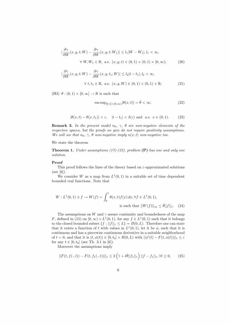
ProofThis proof follows the lines of the theory based on ε-approximated solutions

(see [6]).We consider W as a map from L1(0, 1) in a suitable set of time dependent

bounded real functions. Note that

W : L1(0, 1) ∋ f → W (f) =

∫ 1

0

θ(x, t)f(x) dx,∀f ∈ L1(0, 1),

is such that ||W (f)||∞ ≤ θ||f ||1. (24)

The assumptions on W and γ assure continuity and boundedness of the mapF , defined in (15) on [0,∞)×L1(0, 1), for any f ∈ L1(0, 1) such that it belongsto the closed bounded subset f : ||f ||1 ≤ L = B(0, L). Therefore one can statethat it exists a function of t with values in L1(0, 1), let it be φ, such that it iscontinuous and has a piecewise continuous derivative in a suitable neighborhoodof t = 0, and that it is (t, φ(t)) ∈ [0, t0]×B(0, L) with ||φ′(t)− F (t, φ(t))||1 ≤ εfor any t ∈ [0, t0] (see Th. 3.1 in [6]).

Moreover the assumptions imply

||F (t, f(·, t)) − F (t, f1(·, t))||1 ≤ 2(

γ + lθ||f1||1

)

||f − f1||1,∀t ≥ 0, (25)

6

and consequently if f, f1 ∈ B(f0, r) = f ∈ L1(0, 1) : ||f − f0||1 ≤ r ⊂ B(0, L),the truth of the estimate

||F (t, f(·, t)) − F (t, f1(·, t))||1 ≤ 2(

γ + lθ(||f1||1 + r))

||f − f1||1,∀t ≥ 0. (26)

This inequality imply that two ε1 and ε2-approximated solutions to equation(14), corresponding to the initial values f(·, 0) and f1(·, 0) are such that

||f(·, t)− f1(·, t)||1 ≤ ||f(·, 0)− f1(·, 0)||1 expkt+ (ε1 + ε2)expkt − 1

k. (27)

Here k is the Lipschitz constant of F in the ball B(0, L).Consequently (see Th. 1.6.1 and 1.7.1 of [6]) existence and uniqueness of

the solution of problem (P) can be proved in a suitable bounded closed interval[0, t0].

The fact that the integral of the r.h.s. in (15)

−

∫ 1

0

n(x, t)

∫ 1

0

γ(x, y, t;W ) dy dx +

∫ 1

0

∫ 1

0

γ(y, x, t,W )n(y, t) dy dx = 0, (28)

for any t ≥ 0 in the time interval of existence of the solution, for any n0 ∈L1(0, 1), assure that the solution can be extended to the interval [0,∞).

Remark 4. The solution is such that

∫ 1

0

n(x, t) dx =

∫ 1

0

n0(x) dx,∀t ≥ 0,∀n0 ∈ L1(0, 1). (29)

Remark 5. If γ, θ, n0 are non-negative elements in the respective domains,then the approximated solutions are non-negative; hence the unique solution isnon-negative.

Remark 6. An alternative strategy of proving the existence theorem is based onthe theory of semi-groups of operators. The proofs are essentially generalizationsof the methods of successive approximations which are suitable for nonlinearevolution problems (see e.g. [4], [5]).

Even if proofs are given there for autonomous equations, a careful reader canmodify and fit them to many non autonomous problems. For instance, the caseγ and θ independent of t is well described by the theory exposed in section 3.4and/or 5.4 of [4], and in chapter 3 of [5].

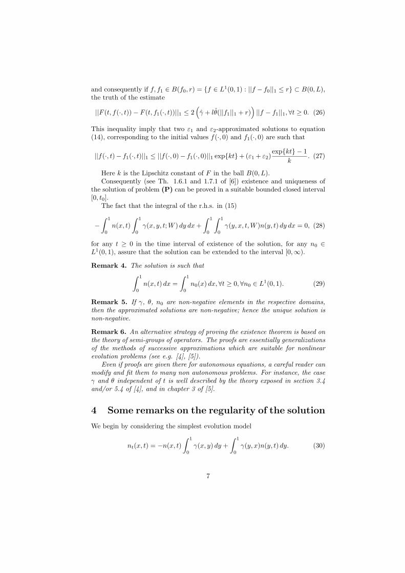
4 Some remarks on the regularity of the solution

We begin by considering the simplest evolution model

nt(x, t) = −n(x, t)

∫ 1

0

γ(x, y) dy +

∫ 1

0

γ(y, x)n(y, t) dy. (30)

7

Theorem 2. If the functions n0(x), γ(x, y) are k-times continuously differen-tiable in [0, 1] and [0, 1]2, respectively, then the unique solution n(x, t) of (30)with the initial condition n(x, 0) = n0(x) has k continuous derivatives with re-spect to x, and all of them are continuously differentiable w.r.t. t.

ProofBy formal differentiation of (30) w.r.t. x we obtain the Cauchy problem

ξt = −ξ(x, t)

∫ 1

0

γ(x, y) dy−n(x, t)

∫ 1

0

γx(x, y) dy+

∫ 1

0

γy(y, x)n(y, t) dy, (31)

ξ(x, 0) = n′

0(x), (32)

where n(x, t) is the known solution of (30). Such a problem has a unique so-lution, which is continuous, with a continuous t-derivative and that coincidesnecessarily with nx. Its explicit expression is

nx(x, t) = n′

0(x)e−g(x)t +

∫ t

0

S(x, τ)e−g(x)(t−τ) dτ, (33)

where

g(x) =

∫ 1

0

γ(x, y) dy, (34)

and S(x, y) denotes the free term in (31).Under the differentiability assumptions on n0(x), γ(x, y) the procedure can

be iterated to calculate ∂kxn.

Theorem 3. Under the assumptions of Theorem 1 the function n(x, t) is C∞

w.r.t. t, for almost all x ∈ (0, 1).

ProofFrom Theorem 1 we already know that nt exists and is continuous in t for

x a.e. in (0, 1). Moreover we can write

nt(x, 0) = n1(x) = −n0(x)g(x) +

∫ 1

0

γ(y, x)n0(y) dy. (35)

The function η(x, t) satisfying the Cauchy problem

ηt(x, t) = −η(x, t)g(x) +

∫ 1

0

γ(y, x)η(y, t) dy, (36)

η(x, 0) = n1(x), (37)

which coincides with the original problem for n with the only change of the initialdata, necessarily coincides with nt. Not only it exists, but has the derivative∂2

t n continuous in t. Next we can calculate the initial value of

∂2t n(x, 0) = n2(x) = −n1(x)g(x) +

∫ 1

0

γ(y, x)n1(y) dy, (38)

8

and iterate the procedure infinitely many times.In the particular case in which the initial distribution n0(x) is bounded we

can say more.

Theorem 4. If ess supΩ n0(x) ≤ A0 the function n(x, t) is analytic with respectto t, a.e in x.

ProofBesides the function g(x) we define h(x) =

∫ 1

0γ(y, x) dy, and we denote by

g and h the L∞ norm of g, h. From (34) we deduce that |n1| ≤ A0(g + h), and

from (38) that |n2| ≤ A0(g + h)2, and so on. Thus we have the estimates∣

∣∂kt |t=0

∣

∣ ≤ A0(g + h)k, (39)

showing that n(x, t) has a uniformly convergent Taylor expansion for t ≥ 0, a.e.in x. Moreover, we have the estimates

|∂mt | ≤ A0(g + h)me(g+h)t, m = 0, 1, 2, . . . . (40)

Theorems 2, 3 and 4 were proved in the case (30) i.e. when social mobilitydoes not depend on the total wealth W (t).

For the more complicated model

nt(x, t) = −n(x, t)

∫ 1

0

γ(x, y,W (t)) dy +

∫ 1

0

γ(y, x,W (t))n(y, t) dy (41)

W (t) =

∫ 1

0

θ(x)n(x, t) dx (42)

the argument for the differentiability of n w.r.t. x goes exactly as in the prof ofTheorem 2.

Proving higher-order differentiability w.r.t. t is still possible but estimatesof the kind (39) cannot be obtained.

5 Some particular cases

This section will be devoted to the analysis of some qualitative properties ofthe solution of problem (P). To be specific we will consider first the case W -independent that is not so far from the concrete situation3. Then we will discussa case of uniform promotion/relegation depending on W .

The scheme of the session is the following.

5.1 We consider the case in which γ has constant values in the regions A =(x, y) : 0 < x < y < 1 and B = (x, y) : 0 < y < x < 1 above and belowthe diagonal of the square (0, 1)2,

3Indeed one can study the problem in a given time interval (say 1-year) and assume thatthe social mobility does not depend on time and corresponds to the total wealth of the societyat the beginning of the period considered. The change of the total wealth can be thought tobe relevant to the social dynamics of the following year.

9

5.2 We allow dependence on just one variable in A and B,

5.3 We consider the symmetric case γ(x, y) = γ(y, x),

5.4 We study the case γ(x, y) = p(x)q(y),

5.5 We consider the case where γ is a given function of W in each of theregions A and B.

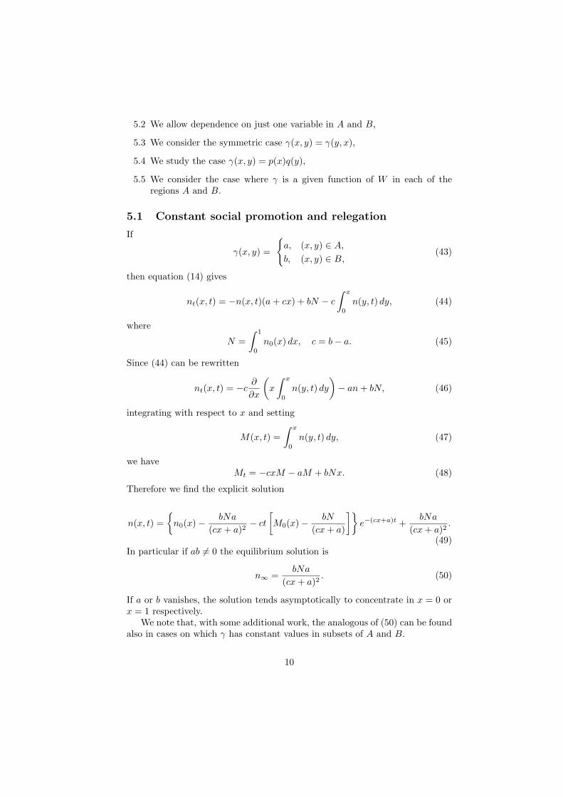
5.1 Constant social promotion and relegation

If

γ(x, y) =

a, (x, y) ∈ A,

b, (x, y) ∈ B,(43)

then equation (14) gives

nt(x, t) = −n(x, t)(a + cx) + bN − c

∫ x

0

n(y, t) dy, (44)

where

N =

∫ 1

0

n0(x) dx, c = b − a. (45)

Since (44) can be rewritten

nt(x, t) = −c∂

∂x

(

x

∫ x

0

n(y, t) dy

)

− an + bN, (46)

integrating with respect to x and setting

M(x, t) =

∫ x

0

n(y, t) dy, (47)

we haveMt = −cxM − aM + bNx. (48)

Therefore we find the explicit solution

n(x, t) =

n0(x) −bNa

(cx + a)2− ct

[

M0(x) −bN

(cx + a)

]

e−(cx+a)t +bNa

(cx + a)2.

(49)In particular if ab 6= 0 the equilibrium solution is

n∞ =bNa

(cx + a)2. (50)

If a or b vanishes, the solution tends asymptotically to concentrate in x = 0 orx = 1 respectively.

We note that, with some additional work, the analogous of (50) can be foundalso in cases on which γ has constant values in subsets of A and B.

10

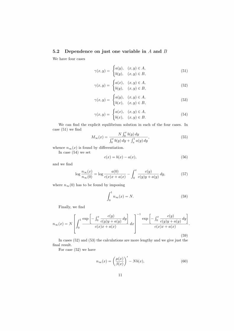
5.2 Dependence on just one variable in A and B

We have four cases

γ(x, y) =

a(y), (x, y) ∈ A,

b(y), (x, y) ∈ B,(51)

γ(x, y) =

a(x), (x, y) ∈ A,

b(y), (x, y) ∈ B,(52)

γ(x, y) =

a(y), (x, y) ∈ A,

b(x), (x, y) ∈ B,(53)

γ(x, y) =

a(x), (x, y) ∈ A,

b(x), (x, y) ∈ B.(54)

We can find the explicit equilibrium solution in each of the four cases. Incase (51) we find

M∞(x) =N

∫ x

0b(y) dy

∫ x

0b(y) dy +

∫ 1

xa(y) dy

, (55)

whence n∞(x) is found by differentiation.In case (54) we set

c(x) = b(x) − a(x), (56)

and we find

logn∞(x)

n∞(0)= log

a(0)

c(x)x + a(x)−

∫ x

0

c(y)

c(y)y + a(y)dy, (57)

where n∞(0) has to be found by imposing

∫ 1

0

n∞(x) = N. (58)

Finally, we find

n∞(x) = N

∫ 1

0

exp

[

−∫ x

0

c(y)

c(y)y + a(y)dy

]

c(x)x + a(x)dx

−1

exp

[

−∫ x

0

c(y)

c(y)y + a(y)dy

]

c(x)x + a(x).

(59)In cases (52) and (53) the calculations are more lengthy and we give just the

final result.For case (52) we have

n∞(x) =

(

µ(x)

β(x)

)

′

− Nb(x), (60)

11

where

µ(x) = (1 − x)

∫ x

0

a′(y)M∞(y) dy, (61)

β(x) =

∫ x

0

b(y) dy + a(x)(1 − x). (62)

For case (53) we define

λ(x) =

∫ 1

x

a(y) dy + xb(x), (63)

ν(x) = λ(x)M∞(x) − N

∫ x

0

b(y) dy, (64)

and we find

ν(x) = N

∫ x

0

x

yexp

∫ x

y

zb′(z)

γ(z)dz

[

1

y

∫ y

0

b(z) dz − b(y)

]

dy. (65)

5.3 The symmetric case γ(x, y) = γ(y, x)

It is immediately verified that in this case we have the constant equilibriumsolution

n∞ = N. (66)

5.4 The case of factorized kernel γ(x, y) = p(x)q(y)

In the particular case p = 1 equation (14) can be written

∂

∂tn(x, t) = −n(x, t)q + q(x)N, (67)

where

q =

∫ 1

0

q(y) dy. (68)

Hence

n(x, t) = n0(x)e−qt +q(x)N

q

(

1 − e−qt)

, (69)

having the asymptotic profile

n∞(x) = q(x)N/q. (70)

In the general factorized case, defining

ν(x) = p(x)n∞(x), (71)

we find that the equilibrium solution n∞ has to satisfy

qν(x) = q(x)ν, (72)

12

where

ν =

∫ 1

0

p(x)n∞(x) dx. (73)

Hence n∞ is given by

n∞(x) = Kq(x)

p(x), (74)

where K is found by imposing that∫ 1

0n∞(x) dx = N

K = N

[∫ 1

0

q(x)

p(x)dx

]−1

. (75)

Of course, we excluded the possibility that p(x) = 0 for some x. But thisfact would mean that there is no possibility of leaving the state x, whereas (ifq(x) 6= 0) there is a finite rate of “arrival” in x from other states. Of course,if x is the unique zero of p(x) the final situation would be n∞(x) = Nδ(x − x)where δ is the Dirac’s delta.

We also note that this result still holds if γ is allowed to depend on W in afactorized form

γ = p(x)q(y)Φ(W ). (76)

Indeed, looking for a stationary solution of (14) Φ(W ) cancels and we areback to the previous case.

5.5 Uniform promotion/relegation rates, depending on W .

Let us go back to the case examined in Sect 5.1, but letting a,b depend on W .Thus we assume

γ(x, y,W ) =

a(W ), (x, y) ∈ A,

b(W ), (x, y) ∈ B,(77)

with a, b continuous and positive for W ∈ [0, N ||θ||], and we look for a steadystate solution4 From Sect. 5.1 we know that if n∞(x) is such a solution, then

n∞(x) = Na(W∞)b(W∞)

[a(W∞) + c(W∞)x]2 , (78)

where W∞ is the wealth index corresponding to n∞(x), namely

W∞ =

∫ 1

0

θ(x)n∞(x) dx. (79)

In the following it will be convenient to define

ω = W∞, H(ω) =b(ω)

a(ω),

4We have seen that the fact that a or b vanish can be associated to singular solutions.

13

so thatc(ω)

a(ω)= H(ω) − 1.

Thus equation (78) can be written as

n∞(x) = NH(ω)

1 + [H(ω) − 1] x2 . (80)

Imposing (79) we conclude that steady state solutions correspond to theroots of the algebraic equation

ω = NH(ω)

∫ 1

0

θ(x)

1 + [H(ω) − 1] x2 dx. (81)

Of course (81) has one unique solution for any θ(x) in the particular case inwhich a and b are proportional, while (81) is identically satisfied for ω = NK0

when θ = K0.We will consider with some more detail the case

θ(x) = λx, (82)

which is, in some sense, the most natural way of associating the wealth indexto the produced wealth W .

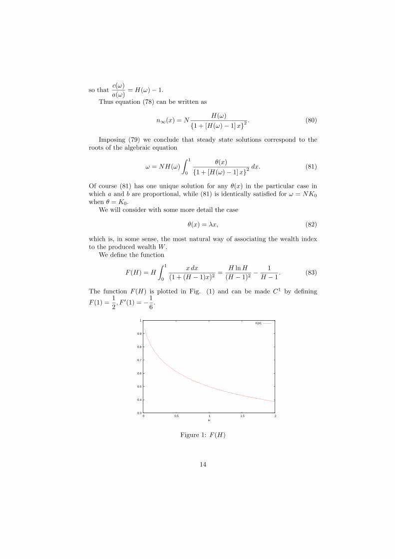
We define the function

F (H) = H

∫ 1

0

x dx

(1 + (H − 1)x)2=

H lnH

(H − 1)2−

1

H − 1. (83)

The function F (H) is plotted in Fig. (1) and can be made C1 by defining

F (1) =1

2, F ′(1) = −

1

6.

0.3

0.4

0.5

0.6

0.7

0.8

0.9

1

0 0.5 1 1.5 2

H

F(H)

Figure 1: F (H)

14

Thus, the solutions of (71) are the values of ω corresponding to the intersec-tion of the curves

y = NλF (H(ω)), (84)

y = ω, (85)

in the strip ω ∈ [0, Nλ] of the (ω, y) plane.Since the range of F in [0, 1] (including also the limit case a(W ) = 0 for

some W ∈ [0, Nλ]) we can conclude that

Proposition 1. In the assumptions (77) there exists at least one solution ofthe problem.

Moreover

Remark 7. IfdH

dW> 1 there exists one and only one stationary solution.

To be specific we consider the following example

a = KW (λN − W ), b = 1, (86)

so that

H(W ) =1

KW (λN − W ), (87)

and we rewrite (81) as1

λNW−1(H) = F (H), (88)

where W−1(H) is the inverse of the function H(W ) and when H is not invertiblewe mean one branch of its inverse graph.

In the example we are considering we have two branches

Ω1(H) =1

2

1 +

√

1 −4

KHλ2N2

, (89)

Ω2(H) =1

2

1 −

√

1 −4

KHλ2N2

, (90)

both defined for H > Hmin =4

Kλ2N2and such that

Ω1(Hmin) = Ω2(Hmin) =1

2. (91)

Note that Ω1 takes values in [1

2, 1] and Ω2 in (0,

1

2] .

We distinguish two cases:

• Hmin ≤ 1,

• Hmin > 1,

15

In the first case the branch Ω1 gives a finite solution, while the branch Ω2 mayhave no finite intersection with the graph of F (H). However it does provide thesolution Ω = 0 (intersection at infinity). This is related (as we have remarkedin Sect. 5.1) with the fact that a(0) = 0.

In the second case we lose the intersection of the first branch, but a finiteintersection will exist with the second branch, since F (H) decays at infinity aslnH

H, while Ω2 decays like

1

KHλ2N2. The intersection at infinity still exists.

0

500

1000

1500

2000

2500

3000

0 0.2 0.4 0.6 0.8 1

t

(a)

230

240

250

260

270

280

290

300

310

320

330

340

0 50 100 150 200

t

(b)

0.76

0.765

0.77

0.775

0.78

0.785

0.79

0.795

0.8

0 50 100 150 200

t

(c)

0 50

100 150

200t 0

0.2

0.4

0.6

0.8

1

x

0

500

1000

1500

2000

2500

3000

(d)

Figure 2: γ as in (93). a: n(x, t) for t = 0 (dotted line), t = 2.0e2 (filled curve);b: W (t); c: ρ(t); d: n(x, t).

6 Some simulations

In this section we will display some numerical simulations that have the sole aimof showing how the model - once calibrated on data taken from some concretesituation - can give some ideas on the social dynamics.

It is commonly accepted that the policy of a society should tend to increasethe total wealth, preserving at the same time some equity.

To measure the latter quantity, several indexes have been proposed. One ofthem is based on the so-called Lorenz curve [13]. In our model it is the curvethat expresses the quantity R(x) =

∫ x

0ξn(ξ) dξ/W with respect to M(x) =

∫ x

0n(ξ) dξ/N .The Gini index (see [9]) is defined as the double of the area between the

16

0

1000

2000

3000

4000

5000

6000

0 0.2 0.4 0.6 0.8 1

t

(a)

330

340

350

360

370

380

390

400

410

0 20 40 60 80 100

t

(b)

0.763

0.764

0.765

0.766

0.767

0.768

0.769

0.77

0.771

0.772

0 20 40 60 80 100

t

(c)

0 20

40 60

80 100

t 0

0.2

0.4

0.6

0.8

1

x

0

1000

2000

3000

4000

5000

6000

(d)

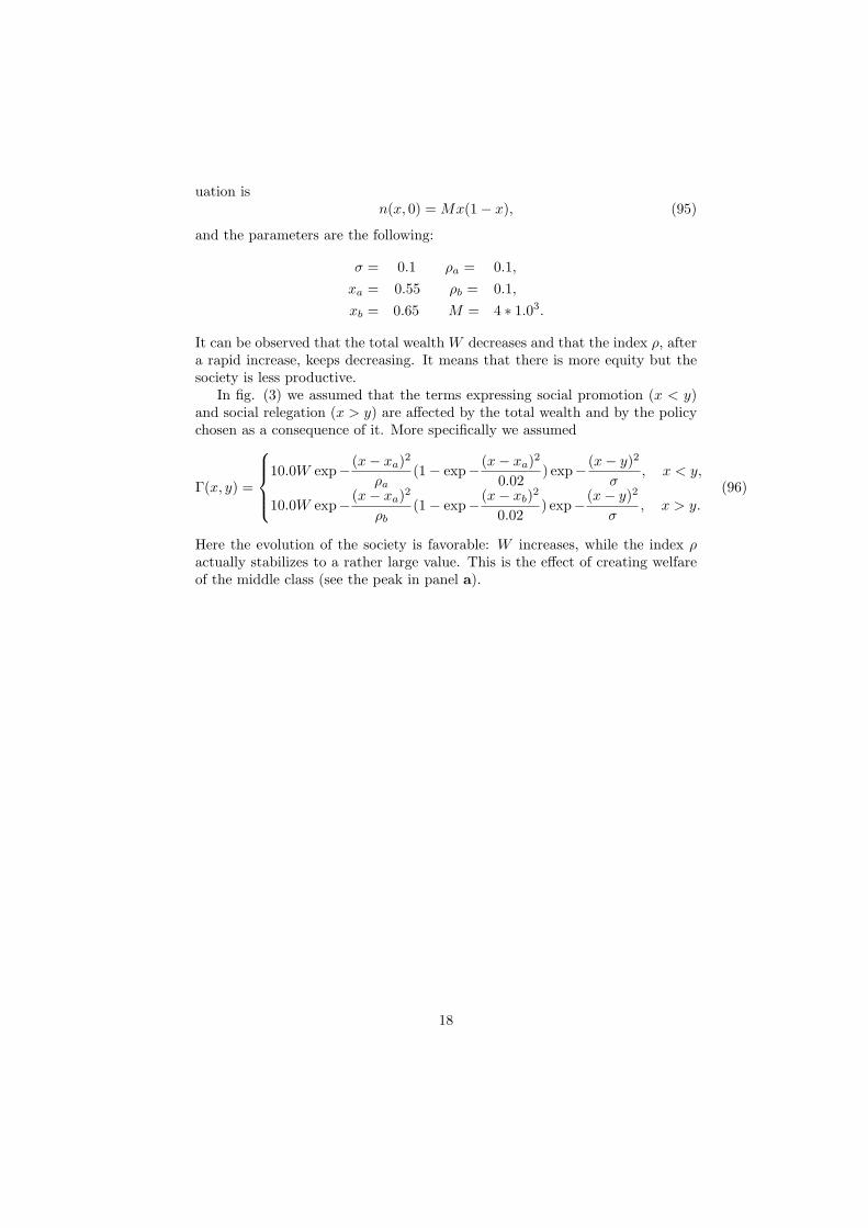
Figure 3: γ as in (96). a: n(x, t) for t = 0 (dotted line), t = 2.0e2 (filled curve);b: W (t); c: ρ(t); d: n(x, t).

diagonal of the two positive axes in the plane (M,R) and the Lorenz curve forthe given society.

It is a number ranging from 0 (total “equity”: a limit case in which all theindividuals have the same individual wealth) to 1 (a limit case in which one hastwo subpopulations of wealth 0 and of wealth 1).

Another possibility of measuring the equity is the fraction of the total wealththat is in the hands - say - the richest 25% of the population: in our notation

ρ = 1 − R(0.75). (92)

Just to have an idea of the dynamics, we have considered the social mobilityof our societies defined as follows

γ(x, y) = exp

[

−−(x − y)2

σ

]

Γ(x, y), (93)

where

Γ(x, y) =

exp−(x − xa)2

ρa

, x < y,

exp−(x − xb)

2

ρb

, x > y.(94)

Fig (2) displays the evolution for different time values where the initial sit-

17

uation isn(x, 0) = Mx(1 − x), (95)

and the parameters are the following:

σ = 0.1 ρa = 0.1,

xa = 0.55 ρb = 0.1,

xb = 0.65 M = 4 ∗ 1.03.

It can be observed that the total wealth W decreases and that the index ρ, aftera rapid increase, keeps decreasing. It means that there is more equity but thesociety is less productive.

In fig. (3) we assumed that the terms expressing social promotion (x < y)and social relegation (x > y) are affected by the total wealth and by the policychosen as a consequence of it. More specifically we assumed

Γ(x, y) =

10.0W exp−(x − xa)2

ρa

(1 − exp−(x − xa)2

0.02) exp−

(x − y)2

σ, x < y,

10.0W exp−(x − xa)2

ρb

(1 − exp−(x − xb)

2

0.02) exp−

(x − y)2

σ, x > y.

(96)

Here the evolution of the society is favorable: W increases, while the index ρactually stabilizes to a rather large value. This is the effect of creating welfareof the middle class (see the peak in panel a).

18

References

[1] http://www.ipam.ucla.edu/programs/chs2007/, 2007.

[2] European Journal of Applied Mathematics, 2010. vol 21, #4-5.

[3] S. Barontini. Popolazioni con strutture sociali e di eta, 2011. Master thesis,Universita di Firenze.

[4] A. Belleni Morante. Applied Semigroups and Evolution Equations. Claren-don Press, Oxford, 1979.

[5] A. Belleni Morante and A.C. McBride. Applied Nonlinear Semigroups.Wiley, 1998.

[6] H. Cartan. Calcul Differentiel. Hermann, Paris, 1967.

[7] H. Caswell. Matrix Population Models: Construction, Analysis and In-terpretation. Sinauer Associates, Sunderland, Massachusetts, 2nd edition,2001.

[8] M. Felson. What every mathematician should know about modelling crime.Eur. J. Appl. Math., 21:275–281, 2010.

[9] C. Gini. Measurement of inequality of incomes. Econ. J., 31(121):124–126,1921.

[10] M.B. Gordon. A random walk in the literature on crominality” a partialand critical view on some statistical analysis and modelling approach. Eur.J. Appl. Math., 21:283–306, 2010.

[11] N Keyfitz. Mathematics and population. SIAM Rev., 15(2):370–375, 1973.

[12] D.O. Logofet and I.N. Belova. Nonnegative matrices as a tool to modelpopulation dynamics: classical models and contemporary expansions. J.Math. Sci., 155:894–907, 2008.

[13] M.O. Lorenz. Methods of measuring the concentration of wealth. Amer.Statistical Assoc., 9:209–219, 1905.

[14] J.C. Nuno, M.A. Herrero, and M. Primicerio. A triangle model of crimi-nality. Physica A, 12(387):2926–2936, 2008.

[15] J.C. Nuno, M.A. Herrero, and M. Primicerio. Fighting cheaters: how andhow much to invest. Eur. J. Appl. Math., 21:459–478, 2010.

[16] J.C. Nuno, M.A. Herrero, and M. Primicerio. A mathematical model of acriminal-prone society. DCDS-S, 4:193–207, 2011.

[17] P. Ormerod, C. Mounfield, and L. Smith. Non-linear modelling of burglaryand violent crime in the UK. Volterra Consulting Ltd, 2001.

19

[18] M.B. Short, P. J. Brantingham, A. L. Bertozzi, and G. E. Tita. Dissipationand displacement of hotspots in reaction-diffusion models of crime. Proc.Nat. Acad. Sci., 107(9):3961–3965, 2010.

[19] D. Usher. The dynastic cycle and the stationary state. Amer. Econ. Rev.,79(5):1031–44, 1989.

[20] L.G. Vargo. A note on crime control. Bull Math Biophys., 28:375–378,1966.

[21] G. F. Webb. Theory of nonlinear age-dependent population dynamics.Dekker, 1985.

20