Models of foreign exchange settlement and informational efficiency

in liquidity risk management

Jochen Schanz*

Bank of England, Financial Resilience Division

Draft, September 2007. Do not quote without the author’s written consent.

The views expressed in this paper are those of the author, and not necessarily those of

the Bank of England.

Abstract: Large, international banking groups have increasingly sought to centralise their cross-currency liquidity management: liquidity shortages in one currency are financed using liquidity surpluses in another currency. We investigate how the degree of coordination in settlement of the associated foreign exchange transactions affects two aspects of banks’ liquidity management: the likelihood that a liquidity-short bank does not meet its obligations but declares technical default, and the likelihood that other banks suffer losses if the liquidity-short bank is also hit by a solvency shock. Our main assumption is that intra-group lending takes place under symmetric information, while interbank market loans are extended under asymmetric information. Better coordinated settlement increases the exposure of the intra-group lender relative to the external lender and leads to more informed lending. We find that better coordination increases the incidence of technical default but reduces the likelihood that solvency shocks are transmitted. * Bank of England, Threadneedle Street, London, EC2R 8AH. E-mail: jochen.schanz@bankofengland.co.uk. I would like to thank Mark Manning, Erlend Nier, Julian Oliver and William Speller for repeated thorough reviews of earlier drafts, and seminar participants at workshops on payment systems and liquidity management at the Bank of England for helpful suggestions. The usual disclaimer applies.

1 Introduction

In 2006, a report by The Joint Forum1 found that �nancial groups have adopted a wide range

of approaches to liquidity risk management in response to greater internationalisation, a de�ning

characteristic of which is the degree of centralisation. Under local liquidity management, each

subsidiary of a �nancial group maintains a separate pool of liquidity in its local currency and funds

its obligations domestically in each market. Under global liquidity management, �nancial groups

also fund liquidity shortfalls (or recycle liquidity surpluses) via intra-group, cross-currency and / or

cross-border transfers of liquidity or collateral: there is a global �ow of liquidity within the group.

In practice, there are many barriers to this global �ow of liquidity. These include: transac-

tion fees; time zone frictions; restrictions on intra-group lending; constraints to accessing intraday

credit at foreign central banks; and a lack of connectivity and harmonisation between the various

national and international payment and settlement systems. We focus on the design of the set-

tlement infrastructure for the cross-currency transfer of liquidity. Would �nancial stability bene�t

from a greater degree of centralisation of liquidity management? And if so, how can the design of

the settlement infrastructure facilitate it? These are current topics of discussions at the Bank for

International Settlement�s Committee for Payment and Settlement Systems (CPSS), and the New

York Fed�s Payments Risk Committee.

A key design feature is the degree of coordination of the settlements of the two currencies which

are exchanged in a foreign exchange (FX) transaction. In July 2007, the CPSS found that an

important share of FX transactions continues to settle �in ways that still generate signi�cant potential

risks across the global �nancial system.� One-third of the $3.8 trillion that settle every day in FX

markets were still subject to such risks. Shocks to an institution could propagate through the

�nancial system: FX exposures to single counterparties typically exceed 5% of an institution�s total

capital in about one-fourth of the institutions on an average day, and in every second institution on a

peak day.2 According to CPSS, one of the reasons for this risk is the absence of complete coordination

of settlement for FX transactions which settle on the day on which they are traded. Such complete

coordination would be o¤ered by a simultaneous (�Payment-versus-Payment�, or PvP) settlement

of both currencies.3 This paper shows that while there are bene�ts to increased coordination for

same-day settlement of foreign exchange transactions, there may also be costs for �nancial stability.

1The Joint Forum (2006)2CPSS (2007, Table 2). The CPSS�s de�nition of total capital is, approximately, equal to the sum of tier 1 capital

(equity and retained earnings), tier 2 capital (supplementary capital) and tier 3 capital (short-term subordinated

debt) as de�ned by the Basel Committee on Banking Supervision.3CLS Bank o¤ers a corresponding service for overnight settlement.

1

Our starting point is the assumption that only external but not internal (within-group) credit

relationships su¤er from asymmetric information between the borrower and the lender. When liq-

uidity is managed locally, a liquidity-short bank has to resort to external �nance. In contrast, when

liquidity is managed globally, such a bank can additionally access foreign-denominated liquidity at

a foreign subsidiary by exchanging it into the home currency. We show that this FX transaction

involves a mixture of external and internal �nance. The higher the degree of coordination in FX

settlement, the larger the share of internal �nance, and the higher the informational e¢ ciency of the

credit relationship. Informational e¢ ciency matters in particular in situations of crises, in which

liquidity is needed on the same day, and in which the lender has little time to evaluate the bor-

rower�s solvency. Indeed, The Joint Forum report found that most �nancial groups expect to rely

upon intra-group, cross-border and cross-currency transfers in stress situations.

We show that the transition from local to global liquidity management, and better coordination of

settlement of FX transactions, have two consequences on �nancial stability. First, the transmission

of solvency shocks from one institution to another would be less likely because banks with high

solvency risks would not be able to re�nance themselves at all in response to liquidity out�ows,

neither domestically nor via FX transactions. But this implies that these banks would have to delay

the payment of their obligations beyond their due-date: they would be in �technical default�. Hence

the second consequence: Technical default might become more likely. These results continue to hold

when we endogenise banks�ex-ante liquidity holdings.

The following section reviews related literature. Sections 3-5 present the model�s setup and guide

the reader through the derivation of the main results. Section 6 shows how these results extend to a

comparison of local with global liquidity management. A discussion of the model�s main assumptions

can be found in section 7. Proofs are presented in the appendix.

2 Related literature

Net redemptions from the banking system are an exception in economies with well-developed �-

nancial markets: if liquidity leaves one bank, it generally �ows via a payment system directly into

the accounts of another bank. If there was no market failure in the domestic interbank market, no

bank would ever experience a liquidity crisis, because it could always re-borrow the liquidity it lost.

Global liquidity management would not have any advantages.

The key assumption in this paper is that there is a market failure in the domestic interbank

market that prevents liquidity from being lent out by a liquidity-rich bank to a liquidity-poor bank.

2

This market failure is due to asymmetric information and was described as a screening problem

by Stiglitz and Weiss (1981). Stiglitz and Weiss argued that borrower/lender relationships are

characterised by asymmetric information. Credit rationing occurs in equilibrium because of two

e¤ects: First, a bank attracts only riskier borrowers when it increases its interest rate (adverse

selection). Second, the borrower might be inclined to increase the risk of his project if the bank

cannot perfectly monitor his choice (moral hazard). Gorton and Huang (2004), Mallick (2004) and

Skeie (2004) suggest other reasons for market failures; but these are more likely to hold for longer-

term exposures. In our model, exposures do not last more than 24 hours; hence our choice to make

adverse selection and not moral hazard the cornerstone of the market imperfection in our model.

Screening problems appear to be very important in reality: banks generally refuse to grant intraday

credit to counterparties which do not have excellent credit status (instead of simply charging them a

higher interest rate); and our market intelligence suggests that even high-quality credit institutions

do not rely on uncollateralised borrowing in their contingency plans.

There are several other strands of models that dealt with related questions. Manning andWillison

(2005) analyse the bene�ts of the cross-border use of collateral in payment systems. In contrast,

we focus on a (more extreme) situation in which banks have no collateralisable assets: thus, banks

have to resort to unsecured borrowing and/or an exchange of foreign currency to transfer their

foreign liquidity holdings into domestic currency. (See section 7 for a discussion.) The literature

on (the limits of) internal capital markets discusses the degree to which internal borrowing takes

place under symmetric information and identi�es a variety of factors that inhibit the information

�ow within a multinational company (e.g., Stein (1997), Scharfstein and Stein (2000)). We abstract

from these frictions to keep the analysis tractable. Kahn and Roberds (2001) describe settlement

banks�incentives in CLS Bank, which started to o¤ered PvP settlement for some foreign exchange

transactions (but not those requiring same-day settlement) in 2002. They argue that PvP increases

the certainty that the counterparty will settle its part of the FX transaction. This improves banks�

incentives to have good liquidity management procedures, but may also reduce their incentive to

monitor counterparties. The authors do not discuss the relative merits of global and local liquidity

management, nor do they show the trade-o¤ between the likelihoods of transmission of shocks and

of technical default. Freixas and Holthausen (2004) study the cross-country integration of interbank

markets. They argue that cross-country interbank market integration may not be perfect when

banks have less knowledge about the solvency of foreign banks. Over the short time-frame we have

in mind, we abstract from the possibility of raising liquidity abroad. Ratnovski (2007) investigates

banks�liquidity holdings under assumptions not unlike our own. In his model, a bank cannot access

3

liquidity held elsewhere within the same group. However, he allows a bank to invest in transparency,

which facilitates the communication of its solvency status when they needs to raise liquidity. We

abstract from investment in communication; if there are serious doubts about a bank�s solvency, this

bank�s statements are unlikely to be believed, and in the short time horizon we focus on a bank is

unlikely to be able to prove its solvency. Fujiki (2006) shows that PvP settlement, together with free

daylight overdrafts from the central bank, is one possibility to yield e¢ ciency gains in an extension

of Freeman�s (1996) island model. Finally, there is a distinct strand of models investigating banks�

reserve management: Tapking (2006) and Ewerhart et al (2004) show that interbank interest rates

do not necessarily have to increase when liquidity becomes scarce. Ho and Saunders (1985) derive

optimal interbank lending to meet reserve requirements.

3 Setup

This section describes the main assumptions (in particular regarding the distribution of information)

and the timing of the game. Figure 1 contains a stylised game tree with the global bank�s most

important decisions. Variables are also listed on page 38 for ease of reference. There are three days

and three players: One global bank with two subsidiaries, GE and GW , and two local banks DE and

DW , one in each country (East or West). Banks are owned by their depositors (equity is zero) and

maximise undiscounted end-of-day-two payo¤s. Local banks are, by assumption, liquidity-rich and

�safe�in that their illiquid assets are not subject to real shocks.

Day zero. The global bank invests its deposits into a risky, illiquid and a risk-free liquid asset.

The risk-free asset pays o¤ one for each unit invested, ie, it has a return of zero. With probability

pi, one unit of the risky asset has a payo¤ of (1 + �) =pi. With probability (1� pi), it becomes

worthless. Thus, one unit of the risky asset is expected to pay o¤ (1 + �); after investment outlays,

the expected pro�t is simply � per unit invested. (Notice that the payo¤ assumptions imply that �

does not depend on pi: this simpli�es the following analysis.) Both pE and pW are distributed as

follows: Either pE = 1, in which case pW is distributed uniformly in [0; 1]; or pW = 1, in which case

pE is distributed uniformly in [0; 1]. Both events have probability 1=2. Their realisations remain the

global bank�s private information. Notice that pE and pW can be interpreted as the likelihood that

a subsidiary�s loan portfolio will not default within the next 24 hours. These probabilities should

generally be very close to one. Thus, it appears justi�able to exclude the case that both portfolios

have a non-zero likelihood of default within the next 24 hours. (See section 7 for a discussion.)

After having learnt the risk of its illiquid assets, the global bank decides how to invest the deposit

4

base of 1 in each country into a risk-free liquid asset (shares LE and LW ) and a risky illiquid asset

(shares 1� LE and 1� LW of its deposit base). The exchange rate between currencies is 1:1.

Nature

Global bank

(pE,pW)

(LE,LW)

Nature

GE is hit byliquidity outflow;GW by an inflow

Global bank (GE) Global bank (GW)

Technicaldefault Refinancing

via o/n loan

Refinancingvia FX swap

Technicaldefault

Refinancingvia o/n loan

(1­LE)ρ­C+(1­LW)ρ

(1­LE)ρ­rDBE+(1­LW)ρ

(1­LE)ρ­rFXBE+(1­LW)ρ

(1­LW)ρ­C+(1­LE)ρ

(1­LW)ρ­rDBW+(1­LE)ρ

GW is hit byliquidity outflow;GE by an inflow

1/2 1/2

Figure 1: The global bank�s main decisions under global liquidity management.

Day one. Banks are hit by liquidity shocks of size �. These liquidity shocks are independent of

pi and sum to zero in two ways: First, if a subsidiary in country i experiences a liquidity out�ow,

the domestic bank in the same country experiences a liquidity in�ow of the same size. This is a

quite natural assumption, given that without central bank intervention, the total amount of central

bank money in an economy remains constant. Second, if a subsidiary in country i experiences a

liquidity out�ow, the subsidiary in the other country j experiences an in�ow of the same size. This

assumption is made to maximise the bene�ts of global liquidity management. It also means that

one subsidiary always has su¢ cient liquidity available to lend out to the other subsidiary, even when

it decides ex ante to hold no liquidity. Thus, the liquidity shock has the following two realisations,

where each has probability 1=2 of occurring:

5

Realisation 1 Realisation 2

GE � ��

GW �� �

DE �� �

DW � ��

In response to the liquidity shock, the global bank has several options. It may have su¢ cient

liquidity to absorb the shock. If, in contrast, there is a shortfall, it may raise BE east dollars (or BW

west dollars, respectively). For its eastern subsidiary, GE , it can choose between re�nancing via a

domestic interbank loan, transferring liquidity between subsidiaries via an FX swap (both with DE

as counterparty), and a declaration that it will have to delay payment until day 2, also referred to

as �technical default�. We assume that the per-dollar cost of the domestic interbank loan, rD, and

the per-dollar cost of the FX swap, rFX , are such that all parties with an exposure to GE expect to

break even. Technical default entails a �xed cost of C, independent of the amount of the payments

that did not settle on day 1: A proxy for the associated reputational damage. (We abstract from

any contagious e¤ect technical default may have on other banks.)

For its western subsidiary, GW , the options are more restricted. This is because of date conven-

tions used in the settlement of foreign exchange transactions explained in more detail in section 5.

The result is that GW only has two options: Technical default and a domestic interbank loan with

DW as counterparty.

Day two. During the subsequent 24 hours, each subsidiary�s illiquid asset may be hit by the

aforementioned real shock. The payo¤s in �gure 1 show expected payo¤s over the possible realisations

of the real shock. If the shock hits a subsidiary, it is forced to default on its obligations, such that its

creditor (if there is one) loses the entire principal amount of its loan. (Notice that this implies that

the illiquid asset cannot be used to collateralise the liquidity-short bank�s loan.) This is referred to

as �transmission of losses�from the debtor to the creditor.

On day 2, if the real shock did not hit Gi�s illiquid asset (probability pi 2 [0; 1]), it pays o¤

su¢ cient liquid assets such that obligations incurred on day 1 can be ful�lled. The assumption

that the asset�s payo¤ is �su¢ cient� is made so as to abstract from repercussions that re�nancing

decisions on day 1 may have for the availability of liquidity on day 2.4 Outstanding interbank loans

are paid back and FX swaps reversed. Each bank distributes its assets among its (local) depositors.

(The need to enter an FX swap rather than just a simple FX transaction is motivated by the latter

4This is clearly a strong simplifation but we would have faced this problem in all games with a �nite number of

periods.

6

assumption).

The following sections �rst derive the optimal liquidity holdings and the likelihood of technical

default and transmission of losses for the base case of symmetric information. The paper�s main

results refer to the case of asymmetric information. Section 4�s results for local liquidity management

are also informative for global liquidity management: as we will argue in section 5, the decisions of

the Western subsidiary are identical in both cases.

4 Local liquidity management

When liquidity is managed locally, each subsidiary of the global bank seeks recourse to the domestic

interbank market if it experiences a liquidity out�ow and does not want to declare technical default.

In market i, it borrows Bi at rate rDi. Its expected payo¤s are independent of the realisation of pi.

This follows from our assumptions that �rst, the risky asset�s return is independent of pi; second,

that the real shock is distributed independently of the liquidity shock; and third, that its potential

lenders only know the prior distribution of pi, such that rDi does not depend on the realisation of

pi. The global bank�s expected payo¤ can be written as

�G = �GE + �GW

= (1� LE) ��1

2pE min fC; rDEBEg

+(1� LW ) ��1

2pW min fC; rDWBW g

where the second line is the expected pro�t from the eastern, and the third line the expected pro�t

from the western subsidiary. (1� Li) � is the expected payo¤ from the illiquid asset, given that a

share (1� Li) of Gi�s balance sheet is invested in it. 12pirDiBi is the expected borrowing cost if

Gi decides to raise funds when short of liquidity (rather than declare technical default). rDiBi, the

interest payment on the loan over Bi, is only made if Gi is still solvent on day 2. This happens

with probability pi. Finally, Gi only su¤ers a liquidity out�ow on day 1 with probability 1=2. If, in

contrast, Gi experiences a liquidity in�ow on day 1, it cannot pro�tably lend out its excess liquidity

on the interbank market because by assumption, the domestic interbank market is already liquidity

rich (i.e., Di does not need to borrow).5 Correspondingly, 12piC is the expected cost of declaring

technical default. (The associated costs C only matter if Gi expects to survive until day 2.)

5 Including a demand for liquidity from a domestic bank would increase the bene�t the global bank derives from

holding liquidity, but not change the dependence between liquidity holding and solvency risk, which is in the focus of

this paper.

7

Two assumptions enable us to solve each subsidiary�s problem independently: Most importantly,

each subsidiary can go bankrupt independently; there are no spillovers from this bankruptcy to the

surviving subsidiary above and beyond a loss resulting from direct credit exposure. (See section 7

for a discussion.) Second, because liquidity management is local in this section, such intra-group

credit exposures never arise. The following results refer to the eastern subsidiary�s decision problem;

the western subsidiary�s are identical.

Because borrowing is costly, GE never borrows more than necessary to cover its liquidity shortfall:

BE � � � LE in all equilibria. Because the cost of technical default is independent of the amount

outstanding at the end of day 1, BE 2 f0; �� LEg in equilibrium: GE either borrows su¢ ciently to

avoid technical default, or nothing at all. If BE = �� LE , its expected pro�t is

�GE (LE ; pE) =

8<: (1� LE) �� 12pErDE (�� LE) if �� C=rDE � LE

(1� LE) �� 12pEC if �� C=rDE > LE

The following lemma shows that the pro�t-maximising ex-ante liquidity holdings must lie in a corner.

Lemma 1 LE 2 f0; �g

Proof. �GE (LE ; pE) is declining in the ex-ante liquidity holding LE with slope � for small

LE � � � C=rD. For larger LE , the slope increases to � + 12pErDE . Thus, �GE (LE ; pE) is convex

in LE .

We also refer to the choice LE = � as �hoarding liquidity�. Whether hoarding liquidity is pro�table

depends, among other factors, on the interest rate rDE which the domestic lender DE charges. By

assumption, liquidity is provided at an interest rate at which DE expects to break even. Break-even

is achieved if

rDE =1� E [pE jpE 2 PDE ]E [pE jpE 2 PDE ]

where PDE is the set of risk types that opt for the interbank loan in equilibrium.

There are three types of equilibria: Those in which PD = ? (either because both the opportunity

costs of holding liquidity and the cost of technical default are low, or because the lender would

expect to face bad risks if, o¤ equilibrium, he was approached for an interbank loan); those in which

PD = [0; 1] (because the opportunity costs of holding liquidity are low, and the cost of technical

default high); and those in which some, but not all risks take out the overnight loan. Lemma 2

provides details.

Lemma 2 GE�s equilibrium strategy ful�ls one of the following:

8

(D1): PD = ?. Then

LE =

8<: 0 if pE � 2��=C

� if pE � 2��=Cand bad risks declare technical default if hit by a liquidity out�ow. This equilibrium exists for all

�, C, and �.

(D2): PD = [0; 2 (1� �)]. Then

LE =

8<: 0 if pE � 2 (1� �)

� if pE � 2 (1� �)

and bad risks take out an overnight loan if hit by a liquidity out�ow. This equilibrium exists if and

only if � � C and � > 1=2.

(D3): PD = [0; 1]. Then LE = 0 for all risks and all risks take out an overnight loan if hit by a

liquidity out�ow. This equilibrium exists if and only if � � C and � > 1=2.

Notice that in both D1 and D2, a bank�s liquidity shortfall is correctly interpreted by the potential

lender as a re�ection of high solvency risk, even though the solvency shock and the liquidity shock

are independent. In case D1, this leads the market to deny credit to the liquidity-short bank. We

abstract from equilibrium D2 because it is unstable, in a sense made more precise in the appendix,

and hence is unlikely to be observed in reality.

The following lemma collects results regarding the ex-ante likelihood of transmission of losses and

technical default under symmetric information for the �stable�equilibria D1 and D3. Transmission

of losses (from GE to its domestic creditor DE) occurs in circumstances in which GE�s illiquid assets

fail (probability (1� pE)) given that GE opted for re�nancing after having been hit by a liquidity

out�ow (probability 1=2). Technical default occurs in circumstances in which GE did not opt for

re�nancing Pr (pE < 2��=C) after having been hit by a liquidity out�ow (probability 1=2).

Lemma 3 Likelihood of technical default and transmission of losses under local liquidity manage-

ment.

1. In equilibrium (D1), the likelihood of transmission of losses is zero. The likelihood of technical

default is1

2Pr (pE � 2��=C) =

��

C

2. In equilibrium (D3), the likelihood of technical default is zero. The likelihood of transmission

of losses is

1

2E [1� pE jpE 2 [0; 1]] Pr (pE 2 [0; 1]) =

1

2

Z 1

0

(1� pE) dpE =1

4

9

Unsurprisingly, the likelihood of technical default is increasing in � (because this increases the

opportunity costs of holding liquidity ex ante) and � (because this makes re�nancing more costly),

and decreasing in C (because for lower C, technical default is associated with a lower penalty).

5 Globally centralised liquidity management

We assume that each subsidiary holds liquidity in its own currency but not in other currencies. A

single unit within the global bank decides on how much liquidity each subsidiary holds. We impose

that intra-group loans of liquidity are charged at an interest rate at which the lender just expects

to break even; a more explicit modelling of the bargaining between lender and borrower is left for

future research. We abstract from regulatory barriers to the transfer of liquidity across jurisdictions

and focus instead on the in�uence the model of settlement of foreign exchange transactions has on

the informational e¢ ciency of the FX market, and thereby on the likelihoods of technical default

and transmission of losses. Importantly, we assume that each subsidiary can default independently,

and that there are no obligations by the surviving part of the global bank to support an insolvent

subsidiary. See section 7 for a discussion.

In reality, an important constraint to foreign exchange trades arises from calendar day conven-

tions. When two banks trade dollars for euros, both the sale and the purchase (the transfer of

dollars and the transfer of euros) have to settle on the same calendar day; otherwise the bank that

receives its payment only on the next calendar day e¤ectively grants the other bank an overnight

loan which is repaid in another currency. This implies that a US subsidiary of a global bank that

�nds itself short of liquidity will not be able to sell euros against dollars without incurring charges

for an overnight loan if the euro payment only settles on the following calendar day. We capture this

asymmetry by assuming that only the eastern subsidiary GE , but not the western subsidiary GW ,

has the option to raise liquidity via an FX transaction.

Because the liquidity shocks are by assumption perfectly negatively correlated across subsidiaries

of the global bank, GW always has su¢ cient liquidity available when GE experiences a liquidity

out�ow. Thus, there is no need for GW to hold ex ante additional liquidity to support GE in case

GE experiences a liquidity out�ow. Equally, GE�s liquidity holdings are independent of GW�s needs

because GW does not have access to FX swaps. This implies that the optimal liquidity holdings

can be derived independently for both subsidiaries and that GW�s optimal liquidity holdings are the

10

same under global and local liquidity management.

Global day 1 Global day 2

GE declared insolventif real shock hits

€ paid to GE $ paid to DE(via DW)

€ repaidto DE

$ repaid toGE (via GW)

Externallender DEhas exposure

Internallender GWhas exposure

Liquidityshock

t 1­t

Risky assetmay pay off

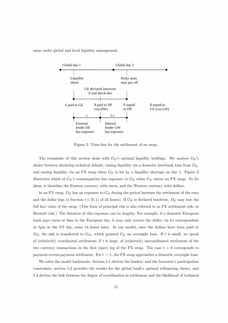
Figure 2: Time-line for the settlement of an swap.

The remainder of this section deals with GE�s optimal liquidity holdings. We analyse GE�s

choice between declaring technical default, raising liquidity via a domestic interbank loan from DE ,

and raising liquidity via an FX swap when GE is hit by a liquidity shortage on day 1. Figure 2

illustrates which of GE�s counterparties has exposure to GE when GE enters an FX swap. To �x

ideas, it identi�es the Eastern currency with euros, and the Western currency with dollars.

In an FX swap, DE has an exposure to GE during the period between the settlement of the euro

and the dollar legs (a fraction t 2 [0; 1) of 24 hours). If GE is declared insolvent, DE may lose the

full face value of the swap. (This form of principal risk is also referred to as FX settlement risk, or

Herstatt risk.) The duration of this exposure can be lengthy: For example, if a domestic European

bank pays euros at 9am in the European day, it may only receive the dollar via its correspondent

at 5pm in the US day, some 14 hours later. In our model, once the dollars have been paid to

DE , the risk is transferred to GW , which granted GE an overnight loan. If t is small, we speak

of (relatively) coordinated settlement; if t is large, of (relatively) uncoordinated settlement of the

two currency transactions in the �rst (spot) leg of the FX swap. The case t = 0 corresponds to

payment-versus-payment settlement. For t! 1, the FX swap approaches a domestic overnight loan.

We solve the model backwards. Section 5.1 derives the lenders�and the borrower�s participation

constraints; section 5.2 provides the results for the global bank�s optimal re�nancing choice, and

5.3 derives the link between the degree of coordination in settlement and the likelihood of technical

11

default and transmission of losses.

5.1 Participation constraints: Determination of the cost of re�nancing

This section derives the lenders� and the borrower�s participation constraints. Consider �rst the

internal lender:

Lemma 4 GW charges the borrower a per-dollar fee of

rG = (1� t)1� pEpE

for the intra-group loan.

Notice that this per-dollar fee is the full-information interest rate appropriate to the borrower�s

risk, (1� pE) =pE , times a factor for the duration of GW�s exposure to GE�s default risk, (1� t). Of

course, the shorter the duration of the exposure, and the lower GE�s risk of default, the lower the

fee. The proof is in the appendix.

The eastern domestic bank, DE , now o¤ers two products: an interbank loan at interest rate rD,

and an FX swap at a fee sD. For the interbank loan, the participation constraint is, as before,

rD �1� E [pjp 2 PI ]E [pjp 2 PI ]

where all pE 2 PI opt for the interbank loan. Lemma 5 provides the corresponding per-dollar fee

for the FX swap:

Lemma 5 As compensation for Herstatt risk, DE charges the borrower a fee of

sD =t (1� E [pjp 2 PFX ])

1� t (1� E [pjp 2 PFX ])

for each unit borrowed, where all pE 2 PFX opt for the FX swap.

This fee is, of course, decreasing in the time t that DE has exposure to GE . It is also decreasing

in DE�s expectation of the borrower�s risk. The proof is in the appendix.

The total per-dollar cost of the FX swap is the sum of both lenders�fees:

rFX (pE ; t; PFX) = (1� t)1� pEpE

+ t

�1� E [pjp 2 PFX ]

1� t (1� E [pjp 2 PFX ])

�Lemma 6 contains comparative static properties:

Lemma 6 For a given PFX 6= ?, the following holds:

12

1. rFX is strictly declining in pE:

@rFX@pE

=@�(1� t) 1�pEpE

+ t�

1�x1�t(1�x)

��@pE

= �1� tp2E

< 0

2. GE�s expected payment for the FX swap, pErFX (pE ; t)BE, is strictly monotone in pE: There

is a unique t0 (PFX) 2 (0; 1] such that

@ (pErFX)

@pE

8>>><>>>:> 0 if t > t0

= 0 if t = t0

< 0 if t < t0

That rFX decreases in pE should be intuitive: A part of the FX transaction is �nanced by an

informed lender, who charges bad risks a higher fee. The strict monotonicity of pErFX (pE ; t) is

important for the structure of the equilibria. A decline in the borrower�s risk has two e¤ects: First,

he is less likely to fail, implying that rFX falls, such that his expected costs of taking out the FX

swap falls. (Recall that only survivors pay.) But for the same reason, he is more likely to have to pay

back the loan, increasing the expected cost of the FX swap. If t is small, both legs of the FX swap

are settled within a short time interval. This implies that the informed lender, GW , carries most of

the exposure. Then rFX declines rapidly in response to better risks, dominating the multiplication

by pE . This case will, in particular, apply for PvP settlement. If, in contrast, t is large, some

time passes until the second currency transaction of the spot leg is settled, such that the external,

uninformed lender carries most of the exposure. The total cost of the FX swap then does not react

much to changes in the borrower�s risk, such that pErFX (pE ; t) is increasing in pE .

5.2 The liquidity-short subsidiary�s re�nancing decision

This section starts out with a presentation of the formal results. The following subsections provide

an intuition.

5.2.1 Equilibrium re�nancing decisions - formal results.

Proposition 1 characterises the forms GE�s equilibrium strategy under global liquidity management.

(There may be additional mixed equilibria for speci�c parameter constellations, e.g., for t = t0; these

are ignored here.)

There are three main classes of equilibria. The �rst two are not able to inform us about global

liquidity management. In the �rst, no loan is made in equilibrium, and the external lender would be

13

very pessimistic about a potential borrower�s risk should he be approached by one. In the second, all

re�nancing is via the interbank loan and no FX swap is o¤ered in equilibrium because the external

lender would be very pessimistic about a potential counterparty�s risk should he be approached

for an FX swap. This type of equilibrium does not appear to be very informative about actual

behaviour because it assumes that DE is happy to take over the exposure to GE overnight, but not

for a fraction of that time.

Of more interest is the third class of equilibria. Here, some re�nancing is carried out via FX

swaps. Proposition 1 shows that if some re�nancing is done via an FX swap (PFX 6= ?), there is

no recourse to overnight loans (PI = ?). Put di¤erently, the model predicts that once the tools

for global liquidity management are in place, a liquidity manager will whenever possible re�nance

himself using internal funds rather than rely on borrowing externally. If the expected return, �, on

the illiquid, risky asset is su¢ ciently high, the liquidity manager will opt to hold no liquid assets

ex ante (equilibria of type G3 in proposition 1 below). Here, good risks will re�nance themselves,

whereas bad risks will opt for technical default if hit by a liquidity out�ow. If, in contrast, the

expected return is low, some risks will opt for hoarding liquidity to avoid borrowing altogether.

Which risks do indeed hold LE = � depends on whether the expected cost of re�nancing via an FX

swap is increasing or decreasing in pE . If pErFX (pE) is strictly increasing in pE (equilibria of type

G4), then the best risks face the highest expected cost of re�nancing (and of technical default), so

they opt for hoarding liquidity. If pErFX (pE) is strictly decreasing in pE (equilibria of type G5),

then the best risks expect to face a relatively low cost of re�nancing via an FX swap, while the worst

risks expect to face a relatively low cost of technical default, such that only the intermediate risks

may have an interest in hoarding liquidity.

Notice that in all equilibria in which there is global re�nancing, the worst risks will prefer to

declare technical default. This is because any FX swap involves at least some portion of informed

lending (t < 1), and because the expected costs, pEC, of the reputational penalty, is very small for

bad risks.

The following two de�nitions will be used:

De�nition 1 Indi¤erent risk types.

p00 : p00 2 [0; 1] and rFX (p00; t; PFX) = C=�

p000 : p000 2 [0; 1] and � = 1

2p000rFX (p

000; t; PFX)

Type p00 is indi¤erent between re�nancing via an FX swap and technical default, given that he

has experienced a liquidity out�ow of size �. All types pE > p00 strictly prefer to re�nance. Type p000

14

is indi¤erent between hoarding liquidity ex ante (and incurring an opportunity cost of �), and relying

on re�nancing via an FX swap should he experience a liquidity out�ow. Notice that, depending on

the equilibrium, PFX may depend on p00 and/or p000, so neither uniqueness nor existence of p00 and

p000 is guaranteed.

Proposition 1 GE�s (Bayesian Nash) equilibrium strategy ful�ls one of the following:

� (G1) No re�nancing: PFX = PI = ? and

LE =

8<: 0 if pE � 2��=C

� if pE � 2��=C

� (G2) Only local re�nancing: PI 6= ? and PFX = ?. Here, the equilibria have the same form

as under local liquidity management.

� Global re�nancing: PFX 6= ?. Then PI = ? and p00 exists and

� Large opportunity cost of holding liquidity:

� G3: If � > prFX (p) =2 for all p > p00, p00 is unique. LE = 0 for all types and

PFX = [p00; 1].

� Small opportunity costs of holding liquidity:

� (G4): If pErFX (pE) is strictly increasing in pE, then for all p000 > p00, PFX = [p00; p000]

and

LE =

8<: 0 if pE � p000

� if pE > p000

G5: If pErFX (pE) is strictly decreasing in pE, then for all p000 > p00, PFX = [p000; 1]

and

LE =

8<: 0 if pE � 2��=C or pE � p000

� if 2��=C < pE < p000

The formal proof can be found in the appendix. As in the case of local liquidity management,

equilibria of the type G4 are unstable in the best-reply dynamic sense. In contrast, equilibria of

types G3 and G5 do not su¤er from this instability.6

Corollary 1 contains speci�c results for the very policy-relevant case of payment-versus-payment

settlement (t = 0). Here, the uninformed lender has no exposure, and information is symmetric.

6To see this, consider equilibria of the form G3 or G5. Here, PFX = [p0; 1] for p0 2 fp00; p000g. A slight exogenous

increase in p0 would improve DE�s expectation and make the FX swap attractive for types below p0 + ", such that p0

would return to equilibrium in a best-reply dynamic.

15

Corollary 1 (PvP settlement) If t = 0,

p00 = �= (�+ C)

p000 = 1� 2�

pErFX (pE) = 1� pE

and there are two equilibria:

� G3 If � >�1� �

C+�

�=2, then PFX = [p00; 1] and LE = 0

� G5 If � <�1� �

C+�

�=2, then PFX = [p000; 1] and

LE =

8<: 0 if pE � 2��=C or pE � p000

� if 2��=C < pE < p000

Notice that for t = 0, pErFX (pE) is strictly decreasing in pE , so G4 does not exist. G1 and G2

also do not exist; in the game under incomplete information (i.e., for t > 0), they owe their existence

to speci�c o¤-equilibrium beliefs.

The following two subsections provide some intuition for the result. The �rst illustrates why

a global liquidity manager generally prefers to re�nance internally. The second shows how the

equilibria of type G3 and G5 are derived.

5.2.2 The availability of an FX swap crowds out re�nancing via domestic overnight

loans.

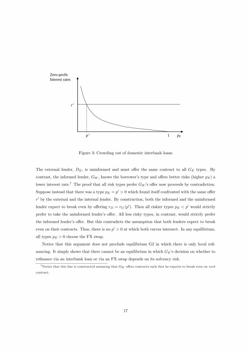
To see why internal re�nancing is preferred, consider �gure 3. It is drawn for a special case, in which

C is high (such that technical default is not an option for any type); � is high (such that GE would

opt to hold no liquidity ex ante independently of its risk), and in which settlement is PvP for the

FX swap (such that GE faces a fully informed counterparty when it enters an FX swap, and an

uninformed counterparty when it re�nances itself domestically). The x-axis shows the likelihood pE

that GE�s illiquid assets pay o¤ on day 2. Thus, GE�s default risk is increasing from the right to the

left. The y-axis shows the interest rates at which GW is willing to grant the intra-group loan (the

downwards sloping line), and the interest rate at which DE is willing to grant the overnight loan

(the horizontal line).

16

1

Zero­profitInterest rates

pE

r’

p’

Figure 3: Crowding out of domestic interbank loans

The external lender, DE , is uninformed and must o¤er the same contract to all GE types. By

contrast, the informed lender, GW , knows the borrower�s type and o¤ers better risks (higher pE) a

lower interest rate.7 The proof that all risk types prefer GW�s o¤er now proceeds by contradiction.

Suppose instead that there was a type pE = p0 > 0 which found itself confronted with the same o¤er

r0 by the external and the internal lender. By construction, both the informed and the uninformed

lender expect to break even by o¤ering rD = rG (p0). Then all riskier types pE < p0 would strictly

prefer to take the uninformed lender�s o¤er. All less risky types, in contrast, would strictly prefer

the informed lender�s o¤er. But this contradicts the assumption that both lenders expect to break

even on their contracts. Thus, there is no p0 > 0 at which both curves intersect. In any equilibrium,

all types pE > 0 choose the FX swap.

Notice that this argument does not preclude equilibrium G2 in which there is only local re�-

nancing. It simply shows that there cannot be an equilibrium in which GE�s decision on whether to

re�nance via an interbank loan or via an FX swap depends on its solvency risk.

7Notice that this line is constructed assuming that GW o¤ers contracts such that he expects to break even on each

contract.

17

5.2.3 Derivation of proposition 1 - intuition

This section provides some graphical intuition for the derivation of equilibria of type G5. Figure 4

shows how the model is solved backwards in this case. It takes the result that the availability of an

FX swap crowds out re�nancing via domestic overnight loans as given.

The �rst panel shows the (second-stage) decision between re�nancing via an FX swap and tech-

nical default. Only good risks (pE � p00) prefer to take out the FX swap. The second panel shows

the (�rst-stage) decision about how much liquidity to hold ex ante. The opportunity cost of hold-

ing liquidity is constant in pE . (This is where the assumption enters that the expected return on

the risky asset is independent of pE .) Re�nancing via an FX swap is preferred by the best risks

(pE � p000). The worst risks (pE � 2��=C) opt for technical default, while intermediate risks prefer

to hoard su¢ cient liquidity to avoid any borrowing. The third panel summarises the results. The

arrows indicate reactions to a decline in the degree of coordination in FX settlement (an increase

in t). Notice that the equilibrium only exists for su¢ ciently small t < t0; only for these t is the

expected cost of re�nancing via an FX swap a declining function of pE . They ultimately determine

the reaction of the likelihood of technical default and of transmission of losses. Their direction is

proven in the following section, also for equilibria of type G3.

18

Expectedcost ofFX swap

1

1

Cost offinancingoptions

pEp’’

Cost of FX swap

Cost of technicaldefault

Cost offinancingoptions

pE

Opportunity cost ofholding liquidity

Expected cost oftechnical default

p’’’

Second stage: Refinancing decision given that liquidity shock cannot be absorbed

First stage: Optimal liquidity holding, given second­stage refinancing decision.

Equilibrium decisions

1

Sufficient liquidity toabsorb liquidityoutflow

No liquidity andtechnical default

No liquidity andrefinancing via FXswap

2λρ/C

Optimal refinancing decisions for highly coordinated (including PvP) settlement

1­t

Figure 4: Construction of equilibrium G5. Arrows indicate comparative static

reactions to an increase in t (decline in coordination).19

5.3 Likelihood of technical default and of transmission of losses

As argued above, it seems reasonable to focus in the following on equilibria of types G3 and G5.

Lemma 7 describes how the degree of coordination of settlement of FX transactions in�uences

the equilibrium proportion of risks which take out an FX swap. This proportion determines the

likelihoods of technical default and transmission of losses (propositions 2 and 3).

Lemma 7 In all stable equilibria in which there is re�nancing via an FX swap, the total derivatives

of p00 and p000 with respect to t are

dp00

dt= �@rFX (p

00; t)

@t=@rFX (p; t)

@p jp=p00< 0

dp000

dt= �@rFX (p

000; t)

@t=@prFX (p; t)

@p jp=p000< 0

The more time elapses between the settlement of the �rst (euro) and the second (dollar) transac-

tions of the spot leg of the FX swap, the larger the share of exposure born by the uninformed lender,

the lower the fee the worst risk in PFX is charged for the FX swap and hence the more attractive it

is to take out the FX swap. As a result, PFX contains worse risks in equilibrium. Essentially, highly

uncoordinated settlement allows relatively bad risks to hide among the good risks when taking out

an FX swap. Put di¤erently, by introducing PvP settlement, the informed lender carries all the

risk, so he increases the charge for bad risks, which in response opt for other alternatives (technical

default in G3; hoarding liquidity in G5).

Ex ante, the increase in the likelihood that GE takes out an FX swap also increases the like-

lihood of transmission of losses: GE�s insolvency only matters for other banks when GE owes

them money. In the equilibria in which the best risks take out the FX swaps (cases G3 and

G5), losses are transmitted if GE is hit by a liquidity out�ow on day 1 (probability 1=2) and,

given this out�ow, re�nances itself (ex ante with probability Pr (pE 2 [p0; 1]) for p0 2 fp00; p000g) and,

given this re�nancing decision, its risky assets are hit by the real shock; that is, with probability12E [1� pE jpE 2 [p

0; 1]] Pr (pE 2 [p0; 1]). Proposition 2 states the result formally:

Proposition 2 In all stable equilibria in which there is re�nancing via an FX swap, losses are more

likely to be transmitted the less coordinated the FX settlement. Formally, for p0 2 fp00; p000g,

@

@t

�1

2E [1� pE jpE 2 [p0; 1]] Pr (pE 2 [p0; 1])

�=

@

@t

�1

4(1� p0)2

�=1

2(1� p0)

��@p

0

@t

�> 0

20

The distribution between domestic and global transmission of losses is also of interest. If GE�s

default occurs while DE has exposure, losses are contained domestically. If, in contrast, GE�s default

occurs while GW has exposure, losses are transmitted only within the same banking group, but across

countries. Clearly, the likelihood of domestic transmission of losses is increasing in t. In contrast,

the likelihood of global transmission of losses may be declining in t, given that GW has, on average,

exposure to worse risks, but only for a shorter duration.

If GE opts against taking out an FX swap, he may choose to declare technical default instead. In

equilibria of the form G3, GE declares technical default whenever he does not take out the FX swap.

Consequently, the ex-ante likelihood of technical default is falling in t. In equilibria of the form G5,

there may be an intermediate interval of risks (pE 2 [2��=C; p000]) which opt for hoarding liquidity.

If this interval is non-empty, the likelihood of technical default is constant in t: only risks worse

than 2��=C opt for technical default, and none of these parameters depend on t. If, in contrast,

the interval is empty, all risks worse than p000 opt for technical default, and p000 is declining in t. So,

again, the ex-ante likelihood of technical default is falling in t. The following proposition summarises

the results:

Proposition 3 In all stable equilibria in which there is re�nancing via an FX swap, the likelihood

of technical default falls the less coordinated the settlement of the two currency transactions in the

spot leg of the FX swap.

The following pictures illustrate these comparative static properties for a special case in which

C=� = 2 and relatively high opportunity costs of liquidity holdings (� = 20%). For some t, both

equilibria G3 and G5 exist. The reader might want to compare the charts with �gure 4, which is

drawn for a speci�c value of t. Shifting the respective lines in �gure 4 in the directions given by the

21

arrows, that is, increasing t, yields the results in �gures 5.4-5.6.

Equilibrium G3 Equilibrium G5

5.1 Refinancing choice

0%

20%

40%

60%

80%

100%

0 0.1 0.2 0.3 0.4 0.5 0.6 0.7 0.8 0.9 1Degree of miscoordination in FX settlement t

Like

lihoo

d of

 pro

ject

 suc

cess

 (lac

kof

 sol

venc

y ri

sk)p

Technical default

Refinancing via FX swap

5.4 Refinancing choice

0%

20%

40%

60%

80%

100%

0 0.1 0.2 0.3 0.4 0.5 0.6Degree of miscoordination in FX settlement t

Like

lihoo

d of

 pro

ject

 suc

cess

 (lac

k of

solv

ency

 risk

)p

Technical default

Refinancing via FX swap

Liquidity hoarding

5.2 Likelihood of transmission of losses

0%

10%

20%

30%

0 0.1 0.2 0.3 0.4 0.5 0.6 0.7 0.8 0.9 1Degree of miscoordination in FX settlement t

Domestic transmission of losses

Global transmission of losses

5.5 Likelihood of transmission of losses

0%

2%

4%

6%

8%

10%

0 0.1 0.2 0.3 0.4 0.5 0.6Degree of miscoordination in FX settlement t

Domestic trans­mission of losses

Global transmission of losses

5.3 Likelihood of technical default

0%

5%

10%

15%

20%

0 0.1 0.2 0.3 0.4 0.5 0.6 0.7 0.8 0.9 1Degree of miscoordination in FX settlement t

5.6 Likelihood of technical default

0%

5%

10%

15%

20%

25%

0 0.1 0.2 0.3 0.4 0.5 0.6Degree of miscoordination in FX settlement t

Figure 5.1 in the top left panel illustrates that as the degree of miscoordination increases, riskier

borrowers are able to take out the FX swap because the uninformed lender determines a larger part

of the FX swap. For t! 1, the FX swap becomes formally equivalent to a domestic overnight loan,

and equilibrium G3 approaches equilibrium D3 (see lemma 8). As a consequence of the decreased

coordination, the likelihood of transmission of shocks rises. Figure 5.2 splits this up into domestic

and global transmission of losses. Also, as riskier borrowers �nd the FX swap more attractive, the

likelihood of technical default decreases (�gure 5.3).

Figure 5.4 illustrates that because the expected cost of re�nancing via an FX swap is decreasing

in t in equilibrium G5, more re�nancing takes place as t rises. Both the opportunity cost of hoarding

liquidity and the expected costs of technical default are constant in t, which is re�ected in the fact

22

that the line that separates the regions in which the subsidiary opts for liquidity hoarding, and

the one in which it prefers technical default, is horizontal. In contrast to the opportunity cost of

hoarding liquidity, the expected costs of technical default are decreasing in pE . Thus, the worst risks

opt for technical default, whereas intermediate risks hoard liquidity. Figures 5.5 and 5.6 show the

resulting consequences on the transmission of losses and the likelihood of technical default.

It is interesting to see how the likelihood of technical default and transmission of losses react

to a change in the size of the liquidity shock, and the cost of technical default. For the interesting

equilibria G3 and G5, proposition 4 shows that the likelihood of technical default is decreasing the

higher the cost of technical default, and the smaller the liquidity shock. This is intuitive: The smaller

the liquidity shock, the lower the re�nancing costs via an FX swap, so the more likely a liquidity-

short bank is to either hoard liquidity or to re�nance when hit by a liquidity out�ow. But a greater

likelihood of re�nancing also implies that transmission of losses has become more likely. Equally

intuitive, both likelihoods of transmission of losses and technical default rise in the opportunity cost

of hoarding liquidity. The proof is in the appendix.

Proposition 4 In all stable equilibria in which there is re�nancing via an FX swap, the likelihood

of technical default falls and the likelihood of transmission of losses rises in C=�. Both rise in �.

6 Comparison between global and local liquidity manage-

ment

When global liquidity management is introduced, equilibrium D1, in which some types re�nance

domestically, does not survive. This is because some of the lending involved in an FX swap is done

by an informed lender, who can o¤er better terms than an uninformed lender for each level of the

borrower�s risk (see section 5.2). Lemma 8 states that equilibrium D3, in which all risks re�nance

domestically, survives as the limit case when the coordination of FX settlement is close to zero:

Lemma 8 For t! 1, equilibrium G3 converges to D3.

The statement is made more precise and proven in the appendix, but the reader can gather the

intuition from �gure 5.1, which shows that for t ! 1, all risks re�nance via an FX swap, which

is virtually identical to a domestic overnight loan (because the domestic lender holds the exposure

for virtually an entire day). Thus, the results in propositions 2 and 3 are equally applicable for a

comparison between local and global liquidity management: Technical default becomes more likely,

and transmission of losses less likely when we move from local to global liquidity management. A

23

considerable caveat to these statements is, of course, that there are multiple equilibria under global

as well under local liquidity management; it is not certain whether banks would indeed move from

equilibrium D3 to G3 once they switch to global liquidity management.

7 Discussion

This section discusses the implications of some of the key assumptions made in the model.

Absence of reputational contagion. We assume that the Eastern subsidiary�s default only

impacts the Western subsidiary to the extent that the Western subsidiary loses the principal amount

of the intragroup loan. However, in practice, the Western subsidiary would probably su¤er some

reputational damage as well.8 If, in response, the Western subsidiary required a higher compensation

for the intragroup loan, the cost of an FX swap would increase, and domestic interbank lending might

not be crowded out. However, one might also argue that the Western subsidiary would be willing to

lend at a lower rate if the Eastern subsidiary otherwise su¤ered re�nancing problems on the following

day.

If the presence of reputational contagion did not change the price of the FX swap, our results

would presumably still hold with respect to actual losses incurred by the depositors: Reputational

contagion is by de�nition independent of the existence of actual exposures. Should depositors decide

to run the surviving subsidiary, fewer assets could be distributed among them if the surviving

subsidiary had to write o¤ a loan to the failed subsidiary. Also, reputational contagion would

presumably be independent of whether the bank manages its liquidity locally or globally. The

comparison between local and global management would then still hold.

It would probably be interesting to study risks of transmission of losses and technical default in a

model in which both GE and GW are not subsidiaries, but branches, which could not fail separately.

This is left for future research.9

Abstraction from re�nancing via cross-border collateral movements. Another option8Notice that for simplicity, we also abstract from any contagion as a consequence of technical default. This would

have required more detailed modelling of the payment �ows on each day and is left for future research.9Relatedly, notice that we restricted attention to the case that only one subsidiary�s loan portfolio was risky at a

time. This appeared to be justi�able given our focus on risk of imminent failure (ie, within the next 24 hours). If

we allowed both portfolios to default and GW defaults before it takes over the exposure to GE in the FX swap, but

after GE received Eastern dollars from DE , GE would not be able to raise Western dollars in time to pay DE . Then

DE would e¤ectively grant GE an overnight loan and require additional payments. This would raise the costs of the

FX swap for good risks, and reduce it for bad risks of GE . In expectation, more risks might opt to take out the FX

swap, but we do not think that our results would change qualitatively.

24

that banks might have available when managing their liquidity globally is the movement of collateral

across borders. Continuing the example in which the Eastern subsidiary su¤ers a liquidity out�ow,

the Western subsidiary could sell (or repo) West-$ denominated collateral in the domestic market.

The Eastern subsidiary could access this liquidity via an FX swap, exactly as discussed above.

The situation would change if the Eastern subsidiary could use West-$ denominated collateral to

raise liquidity from the Eastern subsidiary. In this case, the Western subsidiary could lend the

Eastern subsidiary the West-$ denominated collateral; this would enable the Eastern subsidiary

to raise liquidity under symmetric information. From a modelling perspective, this corresponds

exactly to the situation of PvP settlement of FX swaps. Thus, widening collateral requirements,

and simplifying the process for cross-border transfer of collateral, could be another policy option to

improve the informational e¢ ciency in global liquidity management.

Opportunity costs of liquidity-rich banks and their bargaining power. We assume that

both the internal lender and the external lender are willing to grant a loan at an interest rate at which

they just break even. It might be desirable to endogenise the bargaining between the liquidity-short

bank and its potential lenders. At the moment, we e¤ectively assume that the liquidity-short bank

has all the bargaining power. Consider for the moment the opposite case in which the liquidity-

short bank has no bargaining power, and the lender(s) make take-it-or-leave-it o¤ers. Proposition 1

would then not hold any more. To see this, consider for simplicity the case of PvP settlement. The

informed lender would charge an interest rate high enough to ensure that the liquidity-short bank

would not declare technical default, i.e. such that

� (1� LE)� pErGBE � � (1� LE)� pEC

holds as an equality, leading to rG = C=BE . Then the cost of an FX swap is constant in pE , and

identical to what the outside lender would charge for a domestic overnight loan: rDE would be set

such that

� (1� LE)� E [pE jpE 2 PI ] rDBE � � (1� LE)� E [pE jpE 2 PI ]C

holds as an equality, leading to rDE = C=BE . In practice, the borrower is likely to have some

bargaining power, such that better risks pay less for an FX swap than worse risks, and proposition

1 would presumably go through as in the extreme case we consider.

The speci�cation of the outside option, that is, of declaring technical default, also has

important consequences for the results we derived. First, we assumed that a bank maximises its

payo¤ at the end of day 2; the cost of technical default incurred on day 1 does not matter for a

bank that is declared bankrupt on day 2. In equilibrium, a bank whose illiquid assets do not pay

25

o¤ has no assets left (it either had zero liquid assets when the liquidity shock hit, or borrowed

only just enough to make all necessary payments). There is no additional penalty depositors could

su¤er from technical default. This assumption implies that if funds are insu¢ cient to absorb the

liquidity shock, the liquidity-short bank either declares technical default or takes out the overnight

loan independently of its risk, because the relative size of the expected borrowing cost pErDBE

and the expected cost of technical default pEC is independent of pE . Second, the assumption that

the costs of failing to raise su¢ cient funds are independent of the amount that a bank falls short

appears reasonable when the alternative is a declaration of technical default. However, it would be

less convincing if one interpreted C as the cost of �re-selling assets; an option that is usually open

to banks. Increasing the banks�action space by allowing them to �re-sell assets appears to be an

interesting extension which is left for future research.

8 Conclusion and future research

We show that the transition from local to global liquidity management, and better coordination of

settlement of FX transactions, have two consequences on �nancial stability. First, the transmission

of solvency shocks from one institution to another would be less likely because banks with high

solvency risks would not be able to re�nance themselves at all in response to liquidity out�ows,

neither domestically nor via FX transactions. But this implies that these banks would have to delay

the payment of their obligations beyond their due-date. Hence the second consequence: Technical

default might become more likely. These results continue to hold when we endogenise banks�ex-ante

liquidity holdings.

The paper could be extended in a number of ways. Most importantly, the second-round e¤ects

of technical default and insolvency could be modelled in more detail. In the current version of the

model, only the bank that declares technical default su¤ers a loss. In practice, other banks might

have expected to receive liquidity from this bank and now �nd themselves short of liquidity as well.

However, given that the total amount of (central bank) liquidity is constant in each system, we

would need a slightly more complex scenario for the liquidity shocks. Similarly, there might be

second-round e¤ects for the solvency shock as well: The equity of the defaulting bank�s creditor is

impaired. It might then be more likely to default on its own liabilities and could �nd it di¢ cult to

fund itself, if necessary, on the following day.

26

9 References

Committee for Payment and Settlement Systems (2007), Progress in reducing foreign exchange

settlement risk, Basel.

Committee for Payment and Settlement Systems (2006), Cross-border collateral arrangements,

Basel.

Ewerhart, Christian et al (2004), Liquidity, information and the overnight rate, ECB Working

Paper No. 378

Flannery, Mark J (1996), Financial Crises, Payment System Problems, and Discount Window

Lending, Journal of Money, Credit and Banking 28 (4), 802-824

Freeman, Scott (1996), The Payment System, Liquidity, and Rediscounting, American Economic

Review 86, 1126-1138.

Fujiki, H. 2006. Institutions of Foreign Exchange Settlement in a Two-Country Model. Journal

of Money Credit and Banking 38 (3), 697-719.

Gorton, Garry and Lixin Huang (2004), Liquidity, E¢ ciency and bank bailouts, American Eco-

nomic Review 94 (3), 455-483

Ho, Thomas S Y and Anthony Saunders (1985), A Micro Model of the Federal Funds Market,

Journal of Finance 40(3), 977-988

Kahn, Charles M., and William, Roberds (2001a). The CLS Bank: A Solution to the Risks

of International Payments Settlements. Carnegie-Rochester Conference Series on Public Policy 54,

191-226.

Mallick, Indrajit (2004), Ine¢ ciency of bilateral bargaining in interbank markets, International

Review of Economics and Finance 13, 43-55

Manning, Mark and Matthew Willison (2005), Modelling the cross-border use of collateral in

payment systems, Bank of England Working Paper No 286

Ratnovski, Lev (2007), Liquidity and transparency in bank risk management, mimeo, Bank of

England

Rochet, Jean-Charles and Xavier Vives (2004), Coordination failures and the lender of last resort,

Journal of the European Economic Association 2, 1116�1148.

Skeie, David R (2004), Money and modern bank runs, mimeo

Scharfstein, David S. and Jeremy Stein (2000), The dark side of internal capital markets: divi-

sional rent-seeking and ine¢ cient investment, Journal of Finance 55 (6), 2537-2564.

Stein, Jeremy C (1997), Internal Capital Markets and the Competition for Corporate Resources,

Journal of Finance 52 (1), 111-133.

27

Tapking, Jens (2006), Multiple equilibrium overnight rates in a dynamic interbank market game,

Games and Economic Behavior 56, 350-370

10 Appendix

10.1 Proofs

10.1.1 Local liquidity management

Proof of lemma 2 First recall that the (second-stage) decision over borrowing vs technical default

is independent of pE . Thus, abstracting from the special case that all risks are indi¤erent between

these options, either all pE : LE (pE) = 0 declare technical default (such that PD = ?), or all

pE : LE (pE) = 0 take out an interbank loan (such that PD = fpE 2 [0; 1] : LE (pE) = 0g).

1. Suppose PD = ?. This equilibrium always exists given the o¤-equilibrium belief Pr (pE = 0jPD = ?) =

1. Then LE = 0 is preferred over LE = � if (1� 0) �� 12pEC � (1� �) �, such that

LE =

8<: 0 if pE � 2��=C

� if pE � 2��=C

2. Suppose instead PD 6= ?. Then all pE 2 PD prefer holding LE = 0 over holding LE = � if

(1� 0) �� 12pErD (�� 0) � (1� �) � (1)

equivalently, pE � 2�=rD. This is an upper bound to pE , implying that PD must have the

form [0; p0] where p0 � 1. However, such an equilibrium is unstable in the following sense:

Consider the sequences frD (k) ; p0 (k) ; PD (k)g1k=1 where PD (k) = [0; p0 (k)],

rD (k) =1� E [pE jpE 2 PD (k)]E [pE jpE 2 PD (k)]

=1� 1

2 (1� p0 (k))

12 (1� p0 (k))

=2� p0 (k)p0 (k)

and p0 (k + 1) = 2�=p0 (k), starting at p0 (0) = p0. Then

p0 (k + 1)� p0 (k) = 2�p0

2� p0 � p0 = p0 (k)

p0 (k)� 2 (1� �)2� p0 (k)

This di¤erence is strictly positive for all k if p0 (k) > 2 (1� �), and strictly negative for all k

if p0 (k) < 2 (1� �). But given PD (0) = [0; p0 (0)], p0 2 f0; 2 (1� �)g solve 1 as an equality

(and PD 6= ? only if p0 = 2 (1� �)), so p0 (0) = 2 (1� �). Hence, if the initial shock to p0 was

positive (" > 0), the sequence fp0 (k)g1k=1will at some point increase above 1, whereas it will

fall below zero if " < 0.

28

3. Finally, consider an equilibrium in which PD = [0; 1] and there is no p0 which is indi¤erent

between LE = 0 and LE = �. Then rD = 1. This equilibrium exists under two conditions:

�rst, in the second stage of the game, that borrowing is preferred over technical default given

LE = 0:

(1� 0) �� 12pE (1) (�� 0) � (1� 0) ��

1

2pEC

equivalently, � � C, and second, in the �rst stage of the game, that LE = 0 is strictly preferred

over LE = � for all pE 2 [0; 1], i.e., that

(1� 0) �� 12pE (1) (�� 0) > (1� �) �

equivalently, 2� > pE holds for all types, so also for pE = 1, so this equilibrium exists if

� > 1=2.

10.1.2 Global liquidity management

Proof of lemma 4 This is very straightforward. If GW does not grant the intragroup loan, his

payo¤ is �GW = (1� LW ) �. If he grants the intragroup loan, and GE defaults, his payo¤ is (notice

that we assume that the occurrence of the real shock is uniformly distributed during the day)

�GW = Pr (GE defaults while DE has exposure) (1� LW ) �

+Pr (GE defaults while GW has exposure) ((1� LW ) ��BE)

= t (1� LW ) �+ (1� t) ((1� LW ) �� (1� t)BE)

= (1� LW ) �� (1� t)BE

If GE does not default, the payo¤ is �GW = (1� LW ) �+ rGBE . Then GW is willing to grant the

intragroup loan if

(1� pE) ((1� LW ) �� (1� t)BE) + pE ((1� LW ) �+ rGBE) � (1� LW ) �

equivalently, if� (1� pE) (1� t)+pErG � 0. GW�s break-even per-unit fee rG = (1� t) (1� pE) =pEsolves this equation as an equality.

Proof of lemma 5 Assuming that all pE 2 PFX choose the swap, DE�s payo¤s are �DE = sDBEif GE does not default and, if GE defaults,

�DE = Pr (GE defaults while DE has exposure) (�BE)

+Pr (GE defaults while GW has exposure) (sDBE)

= t (�BE) + (1� t) (sDBE)

29

DE is willing to o¤er the FX swap if his expected payo¤ from doing is (at least) equal to zero,

i.e., if

E [(1� pE) (t (�BE) + (1� t) sDBE) + pEsDBE jpE 2 PFX ] � 0

DE�s break-even per-unit fee sD (t) = t (1� E [pjp 2 PFX ]) = (1� t (1� E [pjp 2 PFX ])) solves this

equation as an equality.

Proof of lemma 6 The change of the total expected cost of the FX swap with respect to pE is,

for a given PE , independent of pE :

@pErFX@pE

= � (1� t) + t�

1� E [pjp 2 PFX ]1� t (1� E [pjp 2 PFX ])

�This implies that the expected costs of an FX swap are monotone in pE for all pE 2 PFX . This

derivative is positive if

t2 � 3� 2E [pjp 2 PFX ]1� E [pjp 2 PFX ]

t+1

1� E [pjp 2 PFX ]� 0

The solutions to the corresponding quadratic equation are

t1;2 =3� 2E [pjp 2 PFX ]2 (1� E [pjp 2 PFX ])

�

q4 (1� E [pjp 2 PFX ])2 + 12 (1� E [pjp 2 PFX ])

It is straighforward to show that the larger root is always larger than 1. Thus,

@ (pErFX)

@pE

8<: > 0 if t � t2< 0 if t < t2

One can show that the smaller root t2 is strictly increasing in E [pjp 2 PFX ]. Also, t2 2 [0:38; 1]

because

limE[pjp2PFX ]!0

t2 =3� 2 (0)2 (1� 0) �

q4 (1� 0)2 + 12 (1� 0) =

3

2� 12

p5 = 0:38

limE[pjp2PFX ]!1

t2 = limx!1

0@ 3� 2x2 (1� x) �

q4 (1� x)2 + 12 (1� x)

1A = 1

Proof of proposition 1 As with local liquidity management, GE�s expected payo¤s

�GE (LE ; pE) =

8>>><>>>:(1� LE) � if LE � �

(1� LE) �� 12pE min frD; rFXgBE if LE < � and min frD; rFXgBE � C

(1� LE) �� 12pEC if LE < � and min frD; rFXgBE � C

30

are declining in BE because borrowing is costly, BE � �� LE in all equilibria. Because the cost of

technical default is independent of the amount outstanding at the end of day 1, BE 2 f0; �� LEg

in equilibrium: GE either borrows su¢ ciently to avoid technical default, or nothing at all. If

BE = �� LE , then

�GE (LE ; pE) =

8<: (1� LE) �� 12pErD (�� LE) if min frD; rFXg (�� LE) � C

(1� LE) �� 12pEC if min frD; rFXg (�� LE) � C

=

8<: (1� LE) �� 12pE min frD; rFXg (�� LE) if �� C=min frD; rFXg � LE

(1� LE) �� 12pEC if �� C=min frD; rFXg > LE

Let PI be the set of types that opt for an interbank loan, and PFX the set of types that opt

for an FX swap. The following paragraphs establish the existence conditions for the equilibria. The

equilibria are grouped by whether or not some risks choose to re�nance themselves via an FX swap

or an interbank loan: i.e., whether in a certain class of equilibria, PFX and PI are non-empty. For

each of the possible cases, conditions for the existence of such equilibria are derived.

1. Suppose PFX = PI = ?. As in the case of local liquidity management, this equilibrium always

exists if t > 0 given GE�s o¤-equilibrium belief that he faces the worst risk if GE asks for

an interbank loan or an FX swap. Then LE = 0 is preferred over LE = � under the same

conditions as in local liquidity management, and

LE =

8<: 0 if pE � 2��=C

� if pE � 2��=C

2. Suppose PFX 6= ?.

First notice that in all equilibria in which there is global re�nancing, the worst risks will prefer

to declare technical default. This is because any FX swap involves at least some portion of

informed lending (t < 1), and because the expected costs, pEC, of the reputational penalty, is

very small for bad risks. Thus, PFX 6= ? requires that p00 exists.

Proof that PI = ?. Suppose in contrast that in equilibrium, PI 6= ?. For this to be an

equilibrium, we need that rD � rFX (p0E) for any p0E 2 PI . Now rFX is strictly decreasing in

pE , so all pE < p0E strictly prefer the external loan to the FX swap. Thus, for any p0E 2 PI and

p00E 2 PFX , p00E > p0E (in words: If PI 6= ?, in equilibrium the better risks go for the FX swap).

Because all p0E 2 PI take out the interbank loan in equilibrium, all pE < max (PI) also prefer

re�nancing via an interbank loan over technical default. (Recall that the choice between an

interbank loan and technical default is independent of pE .) Because all p0E decided to hold no

31

liquidity ex ante, all pE < max (PI) prefer to hold no liquidity ex ante because their expected

borrowing costs, pErD, are even smaller than the best risk�s in PI , while the opportunity costs

of holding liquidity are constant for all risks. Thus, all pE < max (PI) take out the interbank

loan in equilibrium. (Notice that this uses the assumption that the expected return from the

illiquid asset is independent of pE .) Thus, if PI 6= ?, then PI = [0; p0] for some p0 2 (0; 1].

Now consider pE = p0. p0 is indi¤erent between an interbank loan and the cheaper of his

other two options: an FX swap and technical default. But PI = [0; p0] implies that �rst,

rD > (1� p0) =p0, and second, that sD < (1� p0) =p0 because only risks better than p0 choose

the FX swap. This implies that for all t, rFX (p0) = (1� t) (1� p0) =p0 + tsD < rD. But then

p0 strictly prefers the FX swap over the interbank loan, a contradiction. Thus, we cannot have

PI 6= ? if PFX 6= ?.

Having established that PFX 6= ? implies PI = ?, we can rewrite GE�s expected pro�t as

�GE (LE ; pE) =

8<: (1� LE) �� 12pErFX (�� LE) if �� C=rFX � LE

(1� LE) �� 12pEC if �� C=rFX > LE

For a given PFX 6= ?, rFX does not depend on LE . Then �GE (LE ; pE) is declining in LE

with slope � for small LE � � � C=min frD; rFXg. For larger LE , the slope increases to

�+ 12pE . Thus, in all equilibria in which PFX 6= ?, �GE (LE ; pE) is convex in LE and the LE

that maximises �GE must be a corner solution, i.e., in f0; �g. Clearly, if LE = �, only BE = 0

is optimal. If LE = 0, both BE 2 f0; �g can be optimal depending on whether the costs of

raising liquidity exceed the costs of technical default.

Notice that the calculations of the following paragraphs are illustrated in �gure 4 for the case

that pErFX (pE) is strictly decreasing in pE .

(a) Second stage. Consider the re�nancing decision for those types which do not have enough

liquidity to absorb the liquidity shock. Risk pE prefers re�nancing over technical default

if

(1� 0) �� 12pErFX (pE) (�� 0) � (1� 0) ��

1

2pEC

equivalently, rFX (pE) � C=�. Let P 00 = fp 2 [0; 1] : rFX (p) = C=�g.

(b) First stage. Given the second-round decision, LE = � is preferred if

(1� �) � � max�(1� 0) �� 1

2pErFX (pE) (�� 0) ; (1� 0) ��

1

2pEC

�equivalently, 2�� � pE min f�rFX (pE) ; Cg. Let P 000 = fp 2 [0; 1] : 2�� = pmax f�rFX (p) ; Cgg

32

Notice that we have not shown that P 00 and P 000 contain only one point. This is because rFX

depends on PFX , which, in turn, depends on P 00 and P 000. However, we can say something

about the structure of P 00 and P 000 in all equilibria in which PFX 6= ?: For any PFX 6= ?, rFXis strictly declining in pE . Thus

P 00 = fp00 : p00 2 [0; 1] ; rFX (p00) = C=�g

Also, for any PFX 6= ?, prFX (p) is strictly monotone in p. Thus

P 000 = fp000 : p00 2 [0; 1] ; 2�� = p000min f�rFX (p000) ; Cgg

The following paragraphs simply characterise the equilibria depending on whether P 00 and P 000

are empty. This is done �rst for the case that pErFX (pE) is strictly increasing in pE , and then

for the case that pErFX (pE) is strictly decreasing in pE .

(a) Suppose pErFX (pE) is strictly increasing in pE . Then the expected costs of re�nancing,

and the expected costs of declaring technical default are highest for the best risks. Thus,

in equilibrium, at most the best risks prefer to hold LE = �.

i. P 00 = ?. This may occur for two reasons. First, rFX (p) > C=� for all p. Then

technical default would always be preferred over re�nancing via an FX swap. But

then PFX = ?. Second, rFX (p) < C=� for all p, implying that re�nancing via an

FX swap would always be preferred over technical default. If P 000 6= ?, then all p000

ful�l 2� = p000rFX (p000) and for each p000 there is an equilibrium in which

LE =

8<: 0 if pE � p000

� if pE > p000

and PFX = [0; p000]. If P 000 = ? because for all p 2 [0; 1], 2� > prFX (p), then LE = 0

for all p and PFX = [0; 1]. If P 000 = ? because for all p 2 [0; 1], 2� < prFX (p), there

is no equilibrium in which PFX 6= ?.

ii. P 00 6= ?.

A. Suppose �rst that P 000 = ?. This may occur for two reasons. First, for all p 2

[0; 1], 2�� > pmin f�rFX (p) ; Cg. In this case, the expected costs of re�nancing

or technical default are smaller than the opportunity cost for holding liquidity,

and LE = 0 for all types. For each p00 2 P 00, there is an equilibrium in which

LE = 0 for all types. If a liquidity out�ow occurs, only good risks will re�nance:

P 00 6= ? implies that pEC and pErFX (pE) intersect at least once; also, both are

33

linear in pE , and for bad risks, technical default is expected to be less expensive

than re�nancing because

limpE!0

pEC = 0 < limpE!0

pErFX (pE) = 1� t

Thus, in these equilibria, PFX = [p00; 1]. Second, if P 000 = ? because for all

p 2 [0; 1], 2�� < pmin f�rFX (p) ; Cg, then there is no equilibrium in which

PFX 6= ?.

B. Now suppose that P 000 6= ?. Take any p00 2 P 00, p000 2 P 000. Assume �rst that

p000 < p00. But then PFX = ?: P 00 6= ? implies that pEC and pErFX (pE)

intersect at least once; hence, limpE!0 pEC < limpE!0 pErFX (pE) implies that

pEC < pErFX (pE) for all pE < p00. But by de�nition of p000 and increasingness of

pErFX (pE), all risks pE > p000 prefer to hoard liquidity over re�nancing. Assume

instead that p000 � p00. Then p000 is determined by indi¤erence between LE =

0 cum re�nancing and LE = �; that is, p000 : 2� < p000rFX (p000). Then the

equilibrium takes the form

LE =

8<: 0 if pE � p000

� if pE > p000

and PFX = [p00; p000]. All risks worse than p00 declare technical default if hit by a

liquidity out�ow.

(b) Suppose pErFX (pE) is strictly decreasing in pE . Then the expected costs of re�nancing

are decreasing in pE , and the expected costs of declaring technical default are increasing

in pE . Thus, if PFX 6= ?, then PFX =�pIV ; 1

�for some pIV 2 [0; 1). Then pIV is

determined either by indi¤erence between LE = 0 cum re�nancing and LE = �, or by

indi¤erence between LE = 0 cum re�nancing and LE = 0 cum technical default.

i. P 00 = ?. As above, we need rFX (p) < C=� for all p for PFX 6= ?. Then pIV is

determined by indi¤erence between LE = 0 cum re�nancing and LE = �. LE = �

is preferred if 2� < pErFX (pE), i.e., if pE is su¢ ciently small (recall that here we

assume that pErFX (pE) is strictly decreasing in pE). Thus, pIV = p000 and there is

an equilibrium such that

LE =

8<: 0 if pE � p000

� if pE < p000

and PFX = [p000; 1].

34

ii. P 00 6= ?. pE prefers LE = 0 if 2�� � pE min f�rFX (pE) ; Cg. Strict decreasingness of

pErFX (pE) and strict increasingness of pEC in pE imply that pE min f�rFX (pE) ; Cg

is maximal at p00C. Then there are two cases:

A. First, 2�� > pE min f�rFX (pE) ; Cg for all pE , equivalently, 2�� > p00C (or again

equivalently, 2� > p00rFX (p00)). Then pIV is determined by indi¤erence between

LE = 0 cum re�nancing and LE = 0 cum technical default. LE = 0 for all pE .

Consequently, pIV = p00 and PFX = [p00; 1] and all pE � p00 declare technical

default.

B. Alternatively, there are pE such that 2�� = pE min f�rFX (pE) ; Cg. Then pIV

is determined by indi¤erence between LE = 0 cum re�nancing and LE = �.

Consequently, pIV = p000. In this case, su¢ ciently low pE prefer LE = 0 cum

technical default over LE = � if, as before, pE � 2��=C. (p00 < pIV implies

p000 > 2��=C.) Thus, there is an equilibrium such that

LE =

8<: 0 if pE � 2��=C or pE � p000

� if 2��=C < pE < p000

and PFX = [p000; 1].

3. Finally, suppose PFX = ? and PI 6= ?. This equilibrium only exists for non-PvP settlement

and is supported by the (not very convincing) o¤-equilibrium belief that if GE asks o¤ equi-

librium for an FX swap, DE refuses, believing that it faces the worst risk. Given these beliefs,

the FX swap is essentially unavailable for GE , so the situation is exactly the same as under

local liquidity management. The o¤-equilibrium belief is classi�ed as unconvincing because it

implies that DE is ready to accept an overnight exposure to GE , but not the shorter exposure

it would carry if it granted an FX swap.

Proof of lemma 7 p00 is de�ned by rFX (p00) = C=�. Taking total derivatives yields�@rFX@p

� @ (C=�)@p

�dp+

�@rFX@t

� @ (C=�)@t

�dt =

@rFX@p

dp+@rFX@t

dt = 0

such thatdp00

dt= �@rFX

@t=@rFX@p

p000 is de�ned by p000rFX (p000) = 2�. Taking total derivatives yields�@ (prFX)

@p� @ (2�)

@p

�dp+

�@ (prFX)

@t� @ (2�)

@t

�dt

=@ (prFX)

@pdp+ p

@rFX@t

dt = 0

35

such thatdp000

dt= �@rFX

@t=@prFX@p

The remainder of the proof computes the signs of the derivatives. In the equilibria under consider-

ation, PFX = [p; 1] for p 2 fp00; p000g. Then E [pjp 2 PFX ] = (p+ 1) =2. Then

rFX (p; t) = (1� t)1� pp

+ t

�1� (p+ 1) =2

1� t (1� (p+ 1) =2)

�� Regarding the derivative with respect to p,

@rFX@p

=@�(1� t) 1�pp + t

�1�(p+1)=2

1�t(1�(p+1)=2)

��@p

= � (2� t)(p� 1)2 t2 +

�p2 + 2p� 3

�t+ 2

p2 (�t+ pt+ 2)2< 0

if (p� 1)2 t2 +�p2 + 2p� 3

�t+ 2 > 0, equivalently,

t2 +

�p2 + 2p� 3

�(p� 1)2

t+2

(p� 1)2> 0

This holds always true because the roots of the corresponding quadratic equation

t1;2 = ��p2 + 2p� 3

�2 (p� 1)2

�

vuut (p2 + 2p� 3)2 (p� 1)2

!2� 2

(p� 1)2

are both negative.

� Regarding the derivative with respect to t,

@rFX@t

=@�(1� t) 1�pp + t

�1�(p+1)=2

1�t(1�(p+1)=2)

��@t

= � (1� p) (�t+ pt+ 2)2 � 2p

p (�t+ pt+ 2)2< 0

It is straightforward to show that the right-hand side is negative as intuition suggests: A

decrease in the share of informed lending reduces the costs for the marginal lender. Thus,

dp00

dt= �@rFX

@t=@rFX@p

< 0

� Regarding dp000=dt, in equilibria of type (C5), we have @prFX=@p < 0, so

dp000

dt= �@rFX

@t=@prFX@p

< 0

Proof of proposition 4 p00 is de�ned by rFX (p00) = C=�. Taking total derivatives yields�@rFX@p

� @ (C=�)@p

�dp+

�@rFX@ (C=�)

� @ (C=�)@ (C=�)

�d (C=�) =

@rFX@p

dp� d (C=�) = 0

such thatdp00

d (C=�)= 1=

@rFX@p

< 0

36

p000 is de�ned by 2� = p000rFX (p000). Neither side of this equation depends on C=�. (Also notice

that there is no indirect dependence on C=� via p00: in equilibria of type (C5), PFX = [p000; 1]. C=�

only determines the parameter range of � for which the equilibrium (C5) exists (cf. �gure 4).

From proposition 2, the likelihood of transmission of losses is equal to 14 (1� p

0)2 or p0 2 fp00; p000g.

Thus, the likelihood of transmission of losses is declining in p0, and decreasing in (C=�). From

proposition 1, the likelihood of technical default is Pr (pE < p00) in equilibria of type (C3), and

Pr (pE < 2�= (C=�)) in equilibria of type (C5). Both p00 and 2�= (C=�) are decreasing in C=�,

implying that the likelihood of technical default is decreasing in the cost of technical default, and

increasing in the size of the liquidity shock.

The comparative statics with respect to � are straightforward: � only a¤ects the existence of

equilibrium G3 when � = 12p00rFX (p

00), but not p00; hence, if G3 exists, there is no e¤ect of a

marginal change in � on the likelihood of technical default and transmission of losses. For equilibria

in G5, an increase in � makes hoarding liquidity more expensive. This increases the likelihood of

technical default. Regarding the likelihood of transmission of losses, recall that p000 : p000 2 [0; 1] and

� = 12p000rFX (p

000; t; PFX) and, in G5, PFX = [p000; 1]. Taking total derivatives yields�@prFX@p

� @�@p

�dp+

�@prFX@�

� @�@�

�d� =

@prFX@p

dp� d� = 0

such thatdp000

d�= 1=

@prFX@p

< 0

10.1.3 Proof of lemma 8

G3 converges to D3 in the following sense: For t! 1, G3 exists if and only if D3 exists, and liquidity

holding and re�nancing conditions are identical in the sense that all types that re�nance in G3 also

re�nance in D3.

Using PFX = [p00; 1] and p00 : rFX (p00) = C=�, one can solve explicitly for p00:

p00 = �

�2C + 2�� 5t�+ 2t2�� Ct�

q� (t� 2)

�4C�+ 2�2 � C2t� t�2 + 2C2 � 6Ct�

��2t (C + � (2� t))

Taking limits yields

limt!1

p00 =�� C +

q(C � �)2

2 (C + �)=

8<: 0 if C > �

(�� C) = (�+ C) if C � �

D3 exists if and only if � > prFX (p) =2 for all p > p00. Given p00 < 1, we have t0 < 1 (cf. the

proof of lemma 6), so @pErFX (pE) =@pE < 0. Thus, D3 exists if and only if � > rFX (1) =2. Taking

37

limits wrt t yields

� >1

2limt!1

�(1� t) 1� 1

1+ t

�1� E [pjp 2 PFX ]

1� t (1� E [pjp 2 PFX ])

��

=1

2

0@ 1� 12

�1 + max

n0; ��CC+�

o�1�

�1� 1

2

�1 + max

n0; ��CC+�

o��1A =

1

2

1�maxn0; ��CC+�

o1 + max

n0; ��CC+�

oNow C > � implies that this condition is equal to � > 1=2, which is the condition under which D3

exists. Also, for C > �, limt!1 p00 = 0, such that PFX = [0; 1] = PD and LE = 0 in both equilibria.

That is, for t ! 1, the global bank�s subsidiaries do not hold liquidity in either equilibrium, and if

hit by a liquidity out�ow, they both re�nance independently of their risk using an overnight loan

(or, in G3, an FX swap that is indistinguishable from an overnight loan).

10.2 List of symbols

� DE and DW for the domestic banks in countries E and W ; GE and GW for the subsidiaries

of the global bank.

� � is the size of the liquidity shock

� pE and pW are the likelihoods that the subsidiaries�illiquid assets pay o¤ R=pE (R=pW )

� � is the expected net payo¤of each subsidiary�s illiquid assets (i.e., expected gross return minus

1)

� C is the cost of technical default

� LE and LW : Liquidity holdings of the global bank�s subsidiaries. Total balance sheet size is 1

in period zero.

� BE and BW is the amount the liquidity-short branch borrows.

� rDi is the interest rate the domestic bank Di charges for its loan

� sD is the per-dollar fee the domestic bank requires as compensation for Herstatt risk in an FX

swap

� rG is the intragroup per-dollar fee the liquidity-rich subsidiary charges the liquidity-poor sub-

sidiary as part of the FX swap

38