243
Modern Computer Arithmetic Richard P. Brent and Paul Zimmermann Version 0.5.1 of 5 March 2010
Modern Computer Arithmetic
Richard P. Brent and Paul Zimmermann
Version 0.5.1 of 5 March 2010

iii
Copyright c© 2003-2010 Richard P. Brent and Paul Zimmermann
This electronic version is distributed under the terms and conditions of theCreative Commons license “Attribution-Noncommercial-NoDerivative Works3.0”. You are free to copy, distribute and transmit this bookunder the followingconditions:
• Attribution. You must attribute the work in the manner specified by theauthor or licensor (but not in any way that suggests that theyendorse you oryour use of the work).
• Noncommercial.You may not use this work for commercial purposes.• No Derivative Works. You may not alter, transform, or build upon this
work.
For any reuse or distribution, you must make clear to others the license termsof this work. The best way to do this is with a link to the web page below. Anyof the above conditions can be waived if you get permission from the copyrightholder. Nothing in this license impairs or restricts the author’s moral rights.
For more information about the license, visithttp://creativecommons.org/licenses/by-nc-nd/3.0/
Contents
Preface pageixAcknowledgements xiNotation xiii
1 Integer Arithmetic 11.1 Representation and Notations 11.2 Addition and Subtraction 21.3 Multiplication 3
1.3.1 Naive Multiplication 41.3.2 Karatsuba’s Algorithm 51.3.3 Toom-Cook Multiplication 61.3.4 Use of the Fast Fourier Transform (FFT) 81.3.5 Unbalanced Multiplication 81.3.6 Squaring 111.3.7 Multiplication by a Constant 13
1.4 Division 141.4.1 Naive Division 141.4.2 Divisor Preconditioning 161.4.3 Divide and Conquer Division 181.4.4 Newton’s Method 211.4.5 Exact Division 211.4.6 Only Quotient or Remainder Wanted 221.4.7 Division by a Single Word 231.4.8 Hensel’s Division 24
1.5 Roots 251.5.1 Square Root 251.5.2 k-th Root 271.5.3 Exact Root 28
Contents v
1.6 Greatest Common Divisor 291.6.1 Naive GCD 291.6.2 Extended GCD 321.6.3 Half Binary GCD, Divide and Conquer GCD 33
1.7 Base Conversion 371.7.1 Quadratic Algorithms 371.7.2 Subquadratic Algorithms 38
1.8 Exercises 391.9 Notes and References 44
2 Modular Arithmetic and the FFT 472.1 Representation 47
2.1.1 Classical Representation 472.1.2 Montgomery’s Form 482.1.3 Residue Number Systems 482.1.4 MSB vs LSB Algorithms 492.1.5 Link with Polynomials 49
2.2 Modular Addition and Subtraction 502.3 The Fourier Transform 50
2.3.1 Theoretical Setting 502.3.2 The Fast Fourier Transform 512.3.3 The Schonhage-Strassen Algorithm 55
2.4 Modular Multiplication 582.4.1 Barrett’s Algorithm 582.4.2 Montgomery’s Multiplication 602.4.3 McLaughlin’s Algorithm 642.4.4 Special Moduli 65
2.5 Modular Division and Inversion 652.5.1 Several Inversions at Once 67
2.6 Modular Exponentiation 682.6.1 Binary Exponentiation 702.6.2 Exponentiation With a Larger Base 712.6.3 Sliding Window and Redundant Representation 72
2.7 Chinese Remainder Theorem 732.8 Exercises 752.9 Notes and References 77
3 Floating-Point Arithmetic 813.1 Representation 81
3.1.1 Radix Choice 823.1.2 Exponent Range 83
vi Contents
3.1.3 Special Values 843.1.4 Subnormal Numbers 843.1.5 Encoding 853.1.6 Precision: Local, Global, Operation, Operand 863.1.7 Link to Integers 873.1.8 Ziv’s Algorithm and Error Analysis 883.1.9 Rounding 893.1.10 Strategies 93
3.2 Addition, Subtraction, Comparison 933.2.1 Floating-Point Addition 943.2.2 Floating-Point Subtraction 96
3.3 Multiplication 973.3.1 Integer Multiplication via Complex FFT 1013.3.2 The Middle Product 102
3.4 Reciprocal and Division 1043.4.1 Reciprocal 1043.4.2 Division 108
3.5 Square Root 1133.5.1 Reciprocal Square Root 114
3.6 Conversion 1173.6.1 Floating-Point Output 1173.6.2 Floating-Point Input 120
3.7 Exercises 1203.8 Notes and References 122
4 Elementary and Special Function Evaluation 1274.1 Introduction 1274.2 Newton’s Method 128
4.2.1 Newton’s Method for Inverse Roots 1294.2.2 Newton’s Method for Reciprocals 1304.2.3 Newton’s Method for (Reciprocal) Square Roots 1314.2.4 Newton’s Method for Formal Power Series 1314.2.5 Newton’s Method for Functional Inverses 1324.2.6 Higher Order Newton-like Methods 133
4.3 Argument Reduction 1344.3.1 Repeated Use of a Doubling Formula 1364.3.2 Loss of Precision 1364.3.3 Guard Digits 1374.3.4 Doubling versus Tripling 138
4.4 Power Series 138
Contents vii
4.4.1 Direct Power Series Evaluation 1424.4.2 Power Series With Argument Reduction 1424.4.3 Rectangular Series Splitting 143
4.5 Asymptotic Expansions 1464.6 Continued Fractions 1524.7 Recurrence Relations 154
4.7.1 Evaluation of Bessel Functions 1554.7.2 Evaluation of Bernoulli and Tangent numbers 156
4.8 Arithmetic-Geometric Mean 1604.8.1 Elliptic Integrals 1604.8.2 First AGM Algorithm for the Logarithm 1614.8.3 Theta Functions 1624.8.4 Second AGM Algorithm for the Logarithm 1644.8.5 The Complex AGM 165
4.9 Binary Splitting 1664.9.1 A Binary Splitting Algorithm for sin, cos 1684.9.2 The Bit-Burst Algorithm 169
4.10 Contour Integration 1714.11 Exercises 1734.12 Notes and References 181
5 Implementations and Pointers 1875.1 Software Tools 187
5.1.1 CLN 1875.1.2 GNU MP (GMP) 1875.1.3 MPFQ 1885.1.4 MPFR 1895.1.5 Other Multiple-Precision Packages 1895.1.6 Computational Algebra Packages 190
5.2 Mailing Lists 1915.2.1 The BNIS Mailing List 1915.2.2 The GMP Lists 1925.2.3 The MPFR List 192
5.3 On-line Documents 192Bibliography 195
Index 211Summary of Complexities 227

Preface
This is a book about algorithms for performing arithmetic, and their imple-mentation on modern computers. We are concerned with software more thanhardware — we do not cover computer architecture or the design of com-puter hardware since good books are already available on these topics. Insteadwe focus on algorithms for efficiently performing arithmetic operations suchas addition, multiplication and division, and their connections to topics suchas modular arithmetic, greatest common divisors, the Fast Fourier Transform(FFT), and the computation of special functions.
The algorithms that we present are mainly intended for arbitrary-precisionarithmetic. That is, they are not limited by the computer wordsize of32 or 64
bits, only by the memory and time available for the computation. We considerboth integer and real (floating-point) computations.
The book is divided into four main chapters, plus one short chapter (essen-tially an appendix). Chapter 1 covers integer arithmetic. This has, of course,been considered in many other books and papers. However, there has beenmuch recent progress, inspired in part by the application topublic key cryp-tography, so most of the published books are now partly out ofdate or incom-plete. Our aim is to present the latest developments in a concise manner. At thesame time, we provide a self-contained introduction for thereader who is notan expert in the field.
Chapter 2 is concerned with modular arithmetic and the FFT, and their appli-cations to computer arithmetic. We consider different number representations,fast algorithms for multiplication, division and exponentiation, and the use ofthe Chinese Remainder Theorem (CRT).
Chapter 3 covers floating-point arithmetic. Our concern is with high-precision floating-point arithmetic, implemented in software if the precisionprovided by the hardware (typically IEEE standard53-bit significand) is
x Preface
inadequate. The algorithms described in this chapter focuson correct round-ing, extending the IEEE standard to arbitrary precision.
Chapter 4 deals with the computation, to arbitrary precision, of functionssuch as sqrt, exp, ln, sin, cos, and more generally functionsdefined by powerseries or continued fractions. Of course, the computation of special functions isa huge topic so we have had to be selective. In particular, we have concentratedon methods that are efficient and suitable for arbitrary-precision computations.
The last chapter contains pointers to implementations, useful web sites,mailing lists, and so on. Finally, at the end there is a one-page Summary ofComplexitieswhich should be a usefulaide-memoire.
The chapters are fairly self-contained, so it is possible toread them out oforder. For example, Chapter 4 could be read before Chapters 1–3, and Chapter5 can be consulted at any time. Some topics, such as Newton’s method, ap-pear in different guises in several chapters. Cross-references are given whereappropriate.
For details that are omitted we give pointers in theNotes and Referencessections of each chapter, as well as in the bibliography. We have tried, as faras possible, to keep the main text uncluttered by footnotes and references, somost references are given in theNotes and Referencessections.
The book is intended for anyone interested in the design and implementationof efficient algorithms for computer arithmetic, and more generally efficientnumerical algorithms. We did our best to present algorithmsthat are ready toimplement in your favorite language, while keeping a high-level descriptionand not getting too involved in low-level or machine-dependent details. Analphabetical list of algorithms can be found in the index.
Although the book is not specifically intended as a textbook,it could beused in a graduate course in mathematics or computer science, and for thisreason, as well as to cover topics that could not be discussedat length in thetext, we have included exercises at the end of each chapter. The exercises varyconsiderably in difficulty, from easy to small research projects, but we havenot attempted to assign them a numerical rating. For solutions to the exercises,please contact the authors.
We welcome comments and corrections. Please send them to either of theauthors.
Richard Brent and Paul [email protected]
[email protected] and Nancy, February 2010
Acknowledgements
We thank the French National Institute for Research in Computer Science andControl (INRIA), the Australian National University (ANU), and the Aus-tralian Research Council (ARC), for their support. The bookcould not havebeen written without the contributions of many friends and colleagues, too nu-merous to mention here, but acknowledged in the text and in the Notes andReferencessections at the end of each chapter.
We also thank those who have sent us comments on and corrections to ear-lier versions of this book: Jorg Arndt, Marco Bodrato, Wolfgang Ehrhardt (withspecial thanks), Steven Galbraith, Torbjorn Granlund, Guillaume Hanrot, MarcMezzarobba, Jean-Michel Muller, Denis Roegel, Wolfgang Schmid, ArnoldSchonhage, Sidi Mohamed Sedjelmaci, Emmanuel Thome, and Mark Weze-lenburg. Two anonymous reviewers provided very helpful suggestions.
TheMathematics Genealogy Project(http://www.genealogy.ams.org/ ) and Don Knuth’sThe Art of Computer Programming[143] were usefulresources for details of entries in the index.
We also thank the authors of the LATEX program, which allowed us to pro-duce this book, the authors of thegnuplot program, and the authors of theGNU MP library, which helped us to illustrate several algorithms with concretefigures.
Finally, we acknowledge the contribution of Erin Brent, whofirst suggestedwriting the book; and thank our wives, Judy-anne and Marie, for their patienceand encouragement.

Notation
C set of complex numbersC set of extended complex numbersC ∪ ∞N set of natural numbers (nonnegative integers)N∗ set of positive integersN\0Q set of rational numbersR set of real numbersZ set of integersZ/nZ ring of residues modulonCn set of (real or complex) functions withn continuous derivatives
in the region of interest
ℜ(z) real part of a complex numberzℑ(z) imaginary part of a complex numberz
z conjugate of a complex numberz
|z| Euclidean norm of a complex numberz,or absolute value of a scalarz
Bn Bernoulli numbers,∑
n≥0 Bnzn/n! = z/(ez − 1)
Cn scaled Bernoulli numbers,Cn = B2n/(2n)! ,∑Cnz2n = (z/2)/ tanh(z/2)
Tn tangent numbers,∑
Tnz2n−1/(2n − 1)! = tan z
Hn harmonic number∑n
j=1 1/j (0 if n ≤ 0)
(nk
)binomial coefficient “n choosek” = n!/(k! (n − k)!)
(0 if k < 0 or k > n)
xiv Notation
β “word” base (usually232 or 264) or “radix” (floating-point)n “precision”: number of baseβ digits in an integer or in a
floating-point significand, or a free variableε “machine precision”β1−n/2 or (in complexity bounds)
an arbitrarily small positive constantη smallest positive subnormal number
(x), n(x) rounding of real numberx in precisionn (Definition 3.1.1)ulp(x) for a floating-point numberx, one unit in the last place
M(n) time to multiplyn-bit integers, or polynomials ofdegreen − 1, depending on the context
∼M(n) a functionf(n) such thatf(n)/M(n) → 1 asn → ∞(we sometimes lazily omit the “∼” if the meaning is clear)
M(m,n) time to multiply anm-bit integer by ann-bit integerD(n) time to divide a2n-bit integer by ann-bit integer,
giving quotient and remainderD(m,n) time to divide anm-bit integer by ann-bit integer,
giving quotient and remainder
a|b a is a divisor ofb, that isb = ka for somek ∈ Z
a = b mod m modular equality,m|(a − b)
q ← a div b assignment of integer quotient toq (0 ≤ a − qb < b)r ← a mod b assignment of integer remainder tor (0 ≤ r = a − qb < b)(a, b) greatest common divisor ofa andb(
ab
)or (a|b) Jacobi symbol (b odd and positive)
iff if and only ifi ∧ j bitwiseandof integersi andj,
or logicalandof two Boolean expressionsi ∨ j bitwiseor of integersi andj,
or logicalor of two Boolean expressionsi ⊕ j bitwiseexclusive-orof integersi andj
i ≪ k integeri multiplied by2k
i ≫ k quotient of division of integeri by 2k
a · b, a × b product of scalarsa, b
a ∗ b cyclic convolution of vectorsa, b
ν(n) 2-valuation: largestk such that2k dividesn (ν(0) = ∞)σ(e) length of the shortest addition chain to computee
φ(n) Euler’s totient function,#m : 0 < m ≤ n ∧ (m,n) = 1
Notation xv
deg(A) for a polynomialA, the degree ofAord(A) for a power seriesA =
∑j ajz
j ,ord(A) = minj : aj 6= 0 (ord(0) = +∞)
exp(x) or ex exponential functionln(x) natural logarithmlogb(x) base-b logarithmln(x)/ ln(b)
lg(x) base-2 logarithmln(x)/ ln(2) = log2(x)
log(x) logarithm to any fixed baselogk(x) (log x)k
⌈x⌉ ceiling function,minn ∈ Z : n ≥ x⌊x⌋ floor function,maxn ∈ Z : n ≤ x⌊x⌉ nearest integer function,⌊x + 1/2⌋
sign(n) +1 if n > 0, −1 if n < 0, and0 if n = 0
nbits(n) ⌊lg(n)⌋ + 1 if n > 0, 0 if n = 0
[a, b] closed intervalx ∈ R : a ≤ x ≤ b (empty ifa > b)(a, b) open intervalx ∈ R : a < x < b (empty ifa ≥ b)[a, b), (a, b] half-open intervals,a ≤ x < b, a < x ≤ b respectively
t[a, b] or [a, b]t column vector
(a
b
)
[a, b; c, d] 2 × 2 matrix
(a b
c d
)
aj element of the (forward) Fourier transform of vectora
aj element of the backward Fourier transform of vectora
f(n) = O(g(n)) ∃c, n0 such that|f(n)| ≤ cg(n) for all n ≥ n0
f(n) = Ω(g(n)) ∃c > 0, n0 such that|f(n)| ≥ cg(n) for all n ≥ n0
f(n) = Θ(g(n)) f(n) = O(g(n)) andg(n) = O(f(n))
f(n) ∼ g(n) f(n)/g(n) → 1 asn → ∞f(n) = o(g(n)) f(n)/g(n) → 0 asn → ∞f(n) ≪ g(n) f(n) = O(g(n))
f(n) ≫ g(n) g(n) ≪ f(n)
f(x) ∼ ∑n0 aj/xj f(x) − ∑n
0 aj/xj = o(1/xn) asx → +∞
xvi Notation
123 456 789 123456789 (for large integers, we may use a space afterevery third digit)
xxx.yyyρ a numberxxx.yyy written in baseρ;for example, the decimal number3.25 is 11.012 in binary
ab+
cd+
ef+ · · · continued fractiona/(b + c/(d + e/(f + · · · )))
|A| determinant of a matrixA, e.g.
∣∣∣∣a b
c d
∣∣∣∣ = ad − bc
PV∫ b
af(x) dx Cauchy principal value integral, defined by a limit
if f has a singularity in(a, b)
s || t concatenation of stringss andt
⊲ <text> comment in an algorithm
end of a proof
1
Integer Arithmetic
In this chapter our main topic is integer arithmetic. However, weshall see that many algorithms for polynomial arithmetic are sim-ilar to the corresponding algorithms for integer arithmetic, butsimpler due to the lack of carries in polynomial arithmetic.Con-sider for example addition: the sum of two polynomials of degreen always has degree at mostn, whereas the sum of twon-digitintegers may haven+1 digits. Thus we often describe algorithmsfor polynomials as an aid to understanding the corresponding al-gorithms for integers.
1.1 Representation and Notations
We consider in this chapter algorithms working on integers.We distinguishbetween the logical — or mathematical — representation of aninteger, and itsphysical representation on a computer. Our algorithms are intended for “large”integers — they are not restricted to integers that can be represented in a singlecomputer word.
Several physical representations are possible. We consider here only themost common one, namely a dense representation in a fixed base. Choose anintegralbaseβ > 1. (In case of ambiguity,β will be called theinternal base.)A positive integerA is represented by the lengthn and the digitsai of its baseβ expansion:
A = an−1βn−1 + · · · + a1β + a0,
where0 ≤ ai ≤ β − 1, andan−1 is sometimes assumed to be non-zero.Since the baseβ is usually fixed in a given program, only the lengthn andthe integers(ai)0≤i<n need to be stored. Some common choices forβ are232 on a32-bit computer, or264 on a64-bit machine; other possible choices

2 Integer Arithmetic
are respectively109 and1019 for a decimal representation, or253 when usingdouble-precision floating-point registers. Most algorithms given in this chapterwork in any base; the exceptions are explicitly mentioned.
We assume that the sign is stored separately from the absolute value. Thisis known as the “sign-magnitude” representation. Zero is animportant specialcase; to simplify the algorithms we assume thatn = 0 if A = 0, and we usuallyassume that this case is treated separately.
Except when explicitly mentioned, we assume that all operations areoff-line,i.e., all inputs (resp. outputs) are completely known at thebeginning (resp. end)of the algorithm. Different models includelazyandrelaxedalgorithms, and arediscussed in the Notes and References (§1.9).
1.2 Addition and Subtraction
As an explanatory example, here is an algorithm for integer addition. In thealgorithm,d is acarry bit.
Our algorithms are given in a language which mixes mathematical notationand syntax similar to that found in many high-level computerlanguages. Itshould be straightforward to translate into a language suchas C. Note that“ :=” indicates a definition, and “←” indicates assignment. Line numbers areincluded if we need to refer to individual lines in the description or analysis ofthe algorithm.
Algorithm 1.1 IntegerAddition
Input: A =∑n−1
0 aiβi, B =
∑n−10 biβ
i, carry-in0 ≤ din ≤ 1
Output: C :=∑n−1
0 ciβi and0 ≤ d ≤ 1 such thatA + B + din = dβn + C
1: d ← din
2: for i from 0 to n − 1 do3: s ← ai + bi + d
4: (d, ci) ← (s div β, s mod β)
5: returnC, d.
Let T be the number of different values taken by the data type representingthe coefficientsai, bi. (Clearlyβ ≤ T but equality does not necessarily hold,e.g.,β = 109 andT = 232.) At step 3, the value ofs can be as large as2β − 1,which is not representable ifβ = T . Several workarounds are possible: eitheruse a machine instruction that gives the possible carry ofai +bi; or use the factthat, if a carry occurs inai+bi, then the computed sum — if performed modulo
1.3 Multiplication 3
T — equalst := ai + bi − T < ai; thus comparingt andai will determine ifa carry occurred. A third solution is to keep a bit in reserve,takingβ ≤ T/2.
The subtraction code is very similar. Step 3 simply becomess ← ai−bi+d,whered ∈ −1, 0 is theborrow of the subtraction, and−β ≤ s < β. Theother steps are unchanged, with the invariantA − B + din = dβn + C.
We use thearithmetic complexitymodel, wherecost is measured by thenumber of machine instructions performed, or equivalently(up to a constantfactor) thetimeon a single processor.
Addition and subtraction ofn-word integers costO(n), which is negligiblecompared to the multiplication cost. However, it is worth trying to reduce theconstant factor implicit in thisO(n) cost. We shall see in§1.3 that “fast” mul-tiplication algorithms are obtained by replacing multiplications by additions(usually more additions than the multiplications that theyreplace). Thus, thefaster the additions are, the smaller will be the thresholdsfor changing over tothe “fast” algorithms.
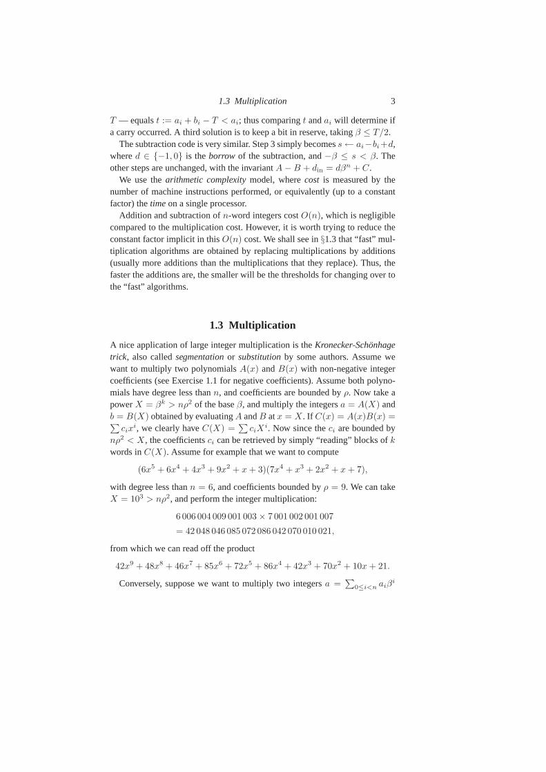
1.3 Multiplication
A nice application of large integer multiplication is theKronecker-Schonhagetrick, also calledsegmentationor substitutionby some authors. Assume wewant to multiply two polynomialsA(x) andB(x) with non-negative integercoefficients (see Exercise 1.1 for negative coefficients). Assume both polyno-mials have degree less thann, and coefficients are bounded byρ. Now take apowerX = βk > nρ2 of the baseβ, and multiply the integersa = A(X) andb = B(X) obtained by evaluatingA andB atx = X. If C(x) = A(x)B(x) =∑
cixi, we clearly haveC(X) =
∑ciX
i. Now since theci are bounded bynρ2 < X, the coefficientsci can be retrieved by simply “reading” blocks ofk
words inC(X). Assume for example that we want to compute
(6x5 + 6x4 + 4x3 + 9x2 + x + 3)(7x4 + x3 + 2x2 + x + 7),
with degree less thann = 6, and coefficients bounded byρ = 9. We can takeX = 103 > nρ2, and perform the integer multiplication:
6 006 004 009 001 003 × 7 001 002 001 007
= 42 048 046 085 072 086 042 070 010 021,
from which we can read off the product
42x9 + 48x8 + 46x7 + 85x6 + 72x5 + 86x4 + 42x3 + 70x2 + 10x + 21.
Conversely, suppose we want to multiply two integersa =∑
0≤i<n aiβi
4 Integer Arithmetic
andb =∑
0≤j<n bjβj . Multiply the polynomialsA(x) =
∑0≤i<n aix
i andB(x) =
∑0≤j<n bjx
j , obtaining a polynomialC(x), then evaluateC(x) atx = β to obtainab. Note that the coefficients ofC(x) may be larger thanβ, infact they may be up to aboutnβ2. For example, witha = 123, b = 456, andβ = 10, we obtainA(x) = x2 + 2x + 3, B(x) = 4x2 + 5x + 6, with productC(x) = 4x4 +13x3 +28x2 +27x+18, andC(10) = 56088. These examplesdemonstrate the analogy between operations on polynomialsand integers, andalso show the limits of the analogy.
A common and very useful notation is to letM(n) denote the time to mul-tiply n-bit integers, or polynomials of degreen− 1, depending on the context.In the polynomial case, we assume that the cost of multiplying coefficients isconstant; this is known as thearithmetic complexitymodel, whereas thebitcomplexitymodel also takes into account the cost of multiplying coefficients,and thus their bit-size.
1.3.1 Naive Multiplication
Algorithm 1.2 BasecaseMultiply
Input: A =∑m−1
0 aiβi, B =
∑n−10 bjβ
j
Output: C = AB :=∑m+n−1
0 ckβk
1: C ← A · b0
2: for j from 1 to n − 1 do3: C ← C + βj(A · bj)
4: returnC.
Theorem 1.3.1 AlgorithmBasecaseMultiplycomputes the productAB cor-rectly, and usesΘ(mn) word operations.
The multiplication byβj at step 3 is trivial with the chosen dense representa-tion: it simply requires shifting byj words towards the most significant words.The main operation in AlgorithmBasecaseMultiply is the computation ofA · bj and its accumulation intoC at step 3. Since all fast algorithms rely onmultiplication, the most important operation to optimize in multiple-precisionsoftware is thus the multiplication of an array ofm words by one word, withaccumulation of the result in another array ofm + 1 words.
We sometimes call AlgorithmBasecaseMultiplyschoolbook multiplicationsince it is close to the “long multiplication” algorithm that used to be taught atschool.
1.3 Multiplication 5
Since multiplication with accumulation usually makes extensive use of thepipeline, it is best to give it arrays that are as long as possible, which meansthatA rather thanB should be the operand of larger size (i.e.,m ≥ n).
1.3.2 Karatsuba’s Algorithm
Karatsuba’s algorithm is a “divide and conquer” algorithm for multiplicationof integers (or polynomials). The idea is to reduce a multiplication of lengthnto three multiplications of lengthn/2, plus some overhead that costsO(n).
In the following,n0 ≥ 2 denotes the threshold between naive multiplica-tion and Karatsuba’s algorithm, which is used forn0-word and larger inputs.The optimal “Karatsuba threshold”n0 can vary from about10 to about100
words, depending on the processor and on the relative cost ofmultiplicationand addition (see Exercise 1.6).
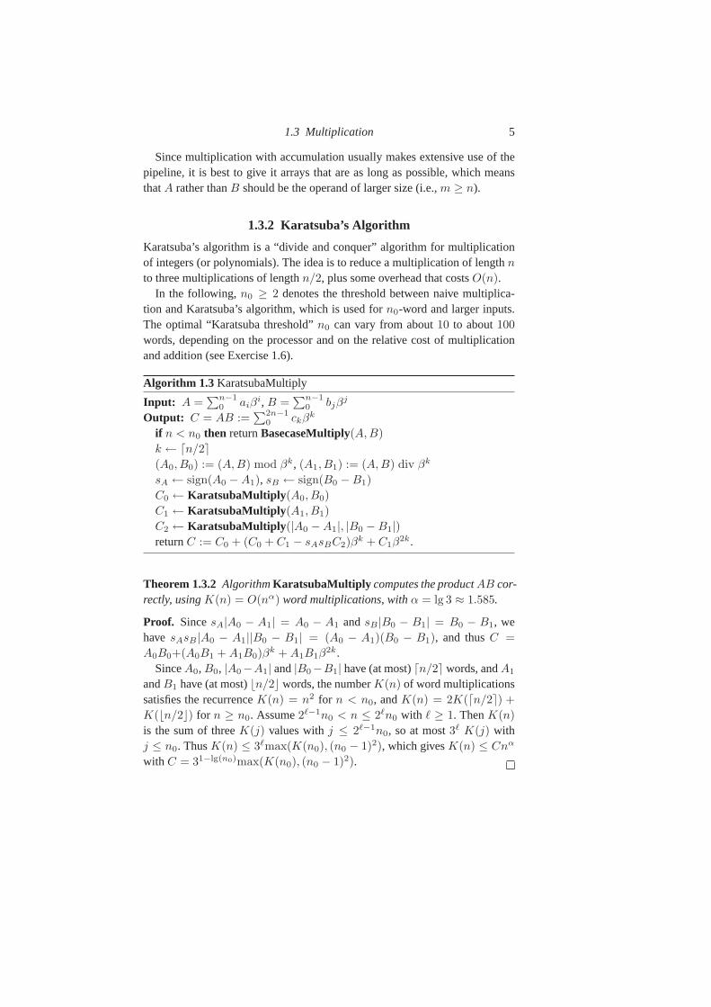
Algorithm 1.3 KaratsubaMultiply
Input: A =∑n−1
0 aiβi, B =
∑n−10 bjβ
j
Output: C = AB :=∑2n−1
0 ckβk
if n < n0 then returnBasecaseMultiply(A,B)
k ← ⌈n/2⌉(A0, B0) := (A,B) mod βk, (A1, B1) := (A,B) div βk
sA ← sign(A0 − A1), sB ← sign(B0 − B1)
C0 ← KaratsubaMultiply (A0, B0)
C1 ← KaratsubaMultiply (A1, B1)
C2 ← KaratsubaMultiply (|A0 − A1|, |B0 − B1|)returnC := C0 + (C0 + C1 − sAsBC2)β
k + C1β2k.
Theorem 1.3.2 AlgorithmKaratsubaMultiply computes the productAB cor-rectly, usingK(n) = O(nα) word multiplications, withα = lg 3 ≈ 1.585.
Proof. SincesA|A0 − A1| = A0 − A1 andsB |B0 − B1| = B0 − B1, wehavesAsB |A0 − A1||B0 − B1| = (A0 − A1)(B0 − B1), and thusC =
A0B0+(A0B1 + A1B0)βk + A1B1β
2k.SinceA0, B0, |A0−A1| and|B0−B1| have (at most)⌈n/2⌉ words, andA1
andB1 have (at most)⌊n/2⌋ words, the numberK(n) of word multiplicationssatisfies the recurrenceK(n) = n2 for n < n0, andK(n) = 2K(⌈n/2⌉) +
K(⌊n/2⌋) for n ≥ n0. Assume2ℓ−1n0 < n ≤ 2ℓn0 with ℓ ≥ 1. ThenK(n)
is the sum of threeK(j) values withj ≤ 2ℓ−1n0, so at most3ℓ K(j) withj ≤ n0. ThusK(n) ≤ 3ℓmax(K(n0), (n0 − 1)2), which givesK(n) ≤ Cnα
with C = 31−lg(n0)max(K(n0), (n0 − 1)2).
6 Integer Arithmetic
Different variants of Karatsuba’s algorithm exist; the variant presented hereis known as thesubtractiveversion. Another classical one is theadditivever-sion, which usesA0+A1 andB0+B1 instead of|A0−A1| and|B0−B1|. How-ever, the subtractive version is more convenient for integer arithmetic, since itavoids the possible carries inA0 + A1 andB0 + B1, which require either anextra word in these sums, or extra additions.
The efficiency of an implementation of Karatsuba’s algorithm depends heav-ily on memory usage. It is important to avoid allocating memory for the inter-mediate results|A0 − A1|, |B0 − B1|, C0, C1, andC2 at each step (althoughmodern compilers are quite good at optimising code and removing unneces-sary memory references). One possible solution is to allow alarge temporarystorage ofm words, used both for the intermediate results and for the recur-sive calls. It can be shown that an auxiliary space ofm = 2n words — or evenm = O(log n) — is sufficient (see Exercises 1.7 and 1.8).
Since the productC2 is used only once, it may be faster to have auxiliaryroutinesKaratsubaAddmul andKaratsubaSubmul that accumulate their re-sult, calling themselves recursively, together withKaratsubaMultiply (seeExercise 1.10).
The version presented here uses∼4n additions (or subtractions):2× (n/2)
to compute|A0 − A1| and |B0 − B1|, thenn to addC0 andC1, againn toadd or subtractC2, andn to add(C0 + C1 − sAsBC2)β
k to C0 + C1β2k. An
improved scheme uses only∼7n/2 additions (see Exercise 1.9).When considered as algorithms on polynomials, most fast multiplication
algorithms can be viewed as evaluation/interpolation algorithms. Karatsuba’salgorithm regards the inputs as polynomialsA0+A1x andB0+B1x evaluatedat x = βk; since their productC(x) is of degree2, Lagrange’s interpolationtheorem says that it is sufficient to evaluateC(x) at three points. The subtrac-tive version evaluates1 C(x) at x = 0,−1,∞, whereas the additive versionusesx = 0,+1,∞.
1.3.3 Toom-Cook Multiplication
Karatsuba’s idea readily generalizes to what is known as Toom-Cookr-waymultiplication. Write the inputs asa0+· · ·+ar−1x
r−1 andb0+· · ·+br−1xr−1,
with x = βk, andk = ⌈n/r⌉. Since their productC(x) is of degree2r − 2,it suffices to evaluate it at2r − 1 distinct points to be able to recoverC(x),and in particularC(βk). If r is chosen optimally, Toom-Cook multiplicationof n-word numbers takes timen1+O(1/
√log n).
1 EvaluatingC(x) at∞ means computing the productA1B1 of the leading coefficients.
1.3 Multiplication 7
Most references, when describing subquadratic multiplication algorithms,only describe Karatsuba and FFT-based algorithms. Nevertheless, the Toom-Cook algorithm is quite interesting in practice.
Toom-Cookr-way reduces onen-word product to2r − 1 products of aboutn/r words, thus costsO(nν) with ν = log(2r − 1)/ log r. However, the con-stant hidden by the big-O notation depends strongly on the evaluation andinterpolation formulæ, which in turn depend on the chosen points. One possi-bility is to take−(r − 1), . . . ,−1, 0, 1, . . . , (r − 1) as evaluation points.
The caser = 2 corresponds to Karatsuba’s algorithm (§1.3.2). The caser =
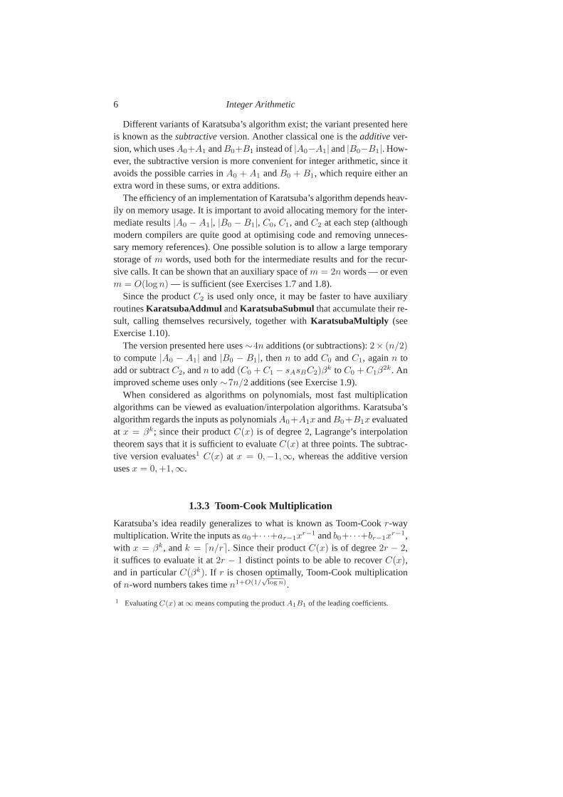
3 is known as Toom-Cook3-way, sometimes simply called “the Toom-Cookalgorithm”. AlgorithmToomCook3uses evaluation points0, 1,−1, 2,∞, andtries to optimize the evaluation and interpolation formulæ.
Algorithm 1.4 ToomCook3Input: two integers0 ≤ A,B < βn
Output: AB := c0 + c1βk + c2β
2k + c3β3k + c4β
4k with k = ⌈n/3⌉Require: a thresholdn1 ≥ 3
1: if n < n1 then returnKaratsubaMultiply (A,B)
2: write A = a0 + a1x + a2x2, B = b0 + b1x + b2x
2 with x = βk.3: v0 ← ToomCook3(a0, b0)
4: v1 ← ToomCook3(a02+a1, b02+b1) wherea02 ← a0+a2, b02 ← b0+b2
5: v−1 ← ToomCook3(a02 − a1, b02 − b1)
6: v2 ← ToomCook3(a0 + 2a1 + 4a2, b0 + 2b1 + 4b2)
7: v∞ ← ToomCook3(a2, b2)
8: t1 ← (3v0 + 2v−1 + v2)/6 − 2v∞, t2 ← (v1 + v−1)/2
9: c0 ← v0, c1 ← v1 − t1, c2 ← t2 − v0 − v∞, c3 ← t1 − t2, c4 ← v∞.
The divisions at step 8 are exact; ifβ is a power of two, the division by6 canbe done using a division by2 — which consists of a single shift — followedby a division by3 (see§1.4.7).
Toom-Cookr-way has to invert a(2r − 1) × (2r − 1) Vandermonde ma-trix with parameters the evaluation points; if one chooses consecutive integerpoints, the determinant of that matrix contains all primes up to 2r − 2. Thisproves that division by (a multiple of)3 can not be avoided for Toom-Cook3-way with consecutive integer points. See Exercise 1.14 fora generalizationof this result.
8 Integer Arithmetic
1.3.4 Use of the Fast Fourier Transform (FFT)
Most subquadratic multiplication algorithms can be seen asevaluation-inter-polation algorithms. They mainly differ in the number of evaluation points, andthe values of those points. However, the evaluation and interpolation formulæbecome intricate in Toom-Cookr-way for larger, since they involveO(r2)
scalar operations. The Fast Fourier Transform (FFT) is a wayto perform eval-uation and interpolation efficiently for some special points (roots of unity) andspecial values ofr. This explains why multiplication algorithms with the bestknown asymptotic complexity are based on the Fast Fourier transform.
There are different flavours of FFT multiplication, depending on the ringwhere the operations are performed. The Schonhage-Strassen algorithm, witha complexity ofO(n log n log log n), works in the ringZ/(2n + 1)Z. Since itis based on modular computations, we describe it in Chapter 2.
Other commonly used algorithms work with floating-point complex num-bers. A drawback is that, due to the inexact nature of floating-point computa-tions, a careful error analysis is required to guarantee thecorrectness of the im-plementation, assuming an underlying arithmetic with rigorous error bounds.See Theorem 3.3.2 in Chapter 3.
We say that multiplication isin the FFT rangeif n is large and the multi-plication algorithm satisfiesM(2n) ∼ 2M(n). For example, this is true if theSchonhage-Strassen multiplication algorithm is used, but notif the classicalalgorithm or Karatsuba’s algorithm is used.
1.3.5 Unbalanced Multiplication
The subquadratic algorithms considered so far (Karatsuba and Toom-Cook)work with equal-size operands. How do we efficiently multiply integers ofdifferent sizes with a subquadratic algorithm? This case isimportant in practicebut is rarely considered in the literature. Assume the larger operand has sizem, and the smaller has sizen ≤ m, and denote byM(m,n) the correspondingmultiplication cost.
If evaluation-interpolation algorithms are used, the costdepends mainly onthe size of the result, that ism+n, so we haveM(m,n) ≤ M((m+n)/2), atleast approximately. We can do better thanM((m+n)/2) if n is much smallerthanm, for exampleM(m, 1) = O(m).
Whenm is an exact multiple ofn, saym = kn, a trivial strategy is to cut thelarger operand intok pieces, givingM(kn, n) = kM(n) + O(kn). However,this is not always the best strategy, see Exercise 1.16.
Whenm is not an exact multiple ofn, several strategies are possible:
1.3 Multiplication 9
• split the two operands into an equal number of pieces of unequal sizes;• or split the two operands into different numbers of pieces.
Each strategy has advantages and disadvantages. We discusseach in turn.
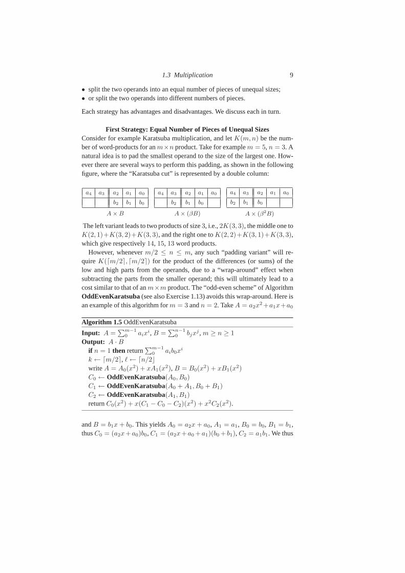
First Strategy: Equal Number of Pieces of Unequal SizesConsider for example Karatsuba multiplication, and letK(m,n) be the num-ber of word-products for anm×n product. Take for examplem = 5, n = 3. Anatural idea is to pad the smallest operand to the size of the largest one. How-ever there are several ways to perform this padding, as shownin the followingfigure, where the “Karatsuba cut” is represented by a double column:
a4 a3 a2 a1 a0
b2 b1 b0
A × B
a4 a3 a2 a1 a0
b2 b1 b0
A × (βB)
a4 a3 a2 a1 a0
b2 b1 b0
A × (β2B)
The left variant leads to two products of size3, i.e.,2K(3, 3), the middle one toK(2, 1)+K(3, 2)+K(3, 3), and the right one toK(2, 2)+K(3, 1)+K(3, 3),which give respectively14, 15, 13 word products.
However, wheneverm/2 ≤ n ≤ m, any such “padding variant” will re-quire K(⌈m/2⌉, ⌈m/2⌉) for the product of the differences (or sums) of thelow and high parts from the operands, due to a “wrap-around” effect whensubtracting the parts from the smaller operand; this will ultimately lead to acost similar to that of anm×m product. The “odd-even scheme” of AlgorithmOddEvenKaratsuba(see also Exercise 1.13) avoids this wrap-around. Here isan example of this algorithm form = 3 andn = 2. TakeA = a2x
2 +a1x+a0
Algorithm 1.5 OddEvenKaratsuba
Input: A =∑m−1
0 aixi, B =
∑n−10 bjx
j , m ≥ n ≥ 1
Output: A · Bif n = 1 then return
∑m−10 aib0x
i
k ← ⌈m/2⌉, ℓ ← ⌈n/2⌋write A = A0(x
2) + xA1(x2), B = B0(x
2) + xB1(x2)
C0 ← OddEvenKaratsuba(A0, B0)
C1 ← OddEvenKaratsuba(A0 + A1, B0 + B1)
C2 ← OddEvenKaratsuba(A1, B1)
returnC0(x2) + x(C1 − C0 − C2)(x
2) + x2C2(x2).
andB = b1x + b0. This yieldsA0 = a2x + a0, A1 = a1, B0 = b0, B1 = b1,thusC0 = (a2x+a0)b0, C1 = (a2x+a0 +a1)(b0 + b1), C2 = a1b1. We thus

10 Integer Arithmetic
getK(3, 2) = 2K(2, 1) + K(1) = 5 with the odd-even scheme. The generalrecurrence for the odd-even scheme is:
K(m,n) = 2K(⌈m/2⌉, ⌈n/2⌉) + K(⌊m/2⌋, ⌊n/2⌋),
instead of
K(m,n) = 2K(⌈m/2⌉, ⌈m/2⌉) + K(⌊m/2⌋, n − ⌈m/2⌉)
for the classical variant, assumingn > m/2. We see that the second parameterin K(·, ·) only depends on the smaller sizen for the odd-even scheme.
As for the classical variant, there are several ways of padding with the odd-even scheme. Considerm = 5, n = 3, and writeA := a4x
4 + a3x3 + a2x
2 +
a1x + a0 = xA1(x2) + A0(x
2), with A1(x) = a3x + a1, A0(x) = a4x2 +
a2x+ a0; andB := b2x2 + b1x+ b0 = xB1(x
2)+B0(x2), with B1(x) = b1,
B0(x) = b2x+b0. Without padding, we writeAB = x2(A1B1)(x2)+x((A0+
A1)(B0 + B1)−A1B1 −A0B0)(x2) + (A0B0)(x
2), which givesK(5, 3) =
K(2, 1) + 2K(3, 2) = 12. With padding, we considerxB = xB′1(x
2) +
B′0(x
2), with B′1(x) = b2x+b0, B′
0 = b1x. This givesK(2, 2) = 3 for A1B′1,
K(3, 2) = 5 for (A0 + A1)(B′0 + B′
1), andK(3, 1) = 3 for A0B′0 — taking
into account the fact thatB′0 has only one non-zero coefficient — thus a total
of 11 only.
Note that when the variablex corresponds to sayβ = 264, AlgorithmOddEvenKaratsuba as presented above is not very practical in the integercase, because of a problem with carries. For example, in the sumA0 + A1 wehave⌊m/2⌋ carries to store. A workaround is to considerx to be sayβ10, inwhich case we have to store only one carry bit for10 words, instead of onecarry bit per word.
The first strategy, which consists in cutting the operands into an equal num-ber of pieces of unequal sizes, does not scale up nicely. Assume for examplethat we want to multiply a number of999 words by another number of699
words, using Toom-Cook3-way. With the classical variant — without padding— and a “large” base ofβ333, we cut the larger operand into three pieces of333 words and the smaller one into two pieces of333 words and one smallpiece of33 words. This gives four full333 × 333 products — ignoring carries— and one unbalanced333 × 33 product (for the evaluation atx = ∞). The“odd-even” variant cuts the larger operand into three pieces of333 words, andthe smaller operand into three pieces of233 words, giving rise to five equallyunbalanced333 × 233 products, again ignoring carries.
1.3 Multiplication 11
Second Strategy: Different Number of Pieces of Equal SizesInstead of splitting unbalanced operands into an equal number of pieces —which are then necessarily of different sizes — an alternative strategy is tosplit the operands into a different number of pieces, and usea multiplicationalgorithm which is naturally unbalanced. Consider again the example of mul-tiplying two numbers of999 and699 words. Assume we have a multiplicationalgorithm, say Toom-(3, 2), which multiplies a number of3n words by anothernumber of2n words; this requires four products of numbers of aboutn words.Usingn = 350, we can split the larger number into two pieces of350 words,and one piece of299 words, and the smaller number into one piece of350
words and one piece of349 words.Similarly, for two inputs of1000 and500 words, we can use a Toom-(4, 2)
algorithm which multiplies two numbers of4n and2n words, withn = 250.Such an algorithm requires five evaluation points; if we choose the same pointsas for Toom3-way, then the interpolation phase can be shared between bothimplementations.
It seems that this second strategy is not compatible with the“odd-even”variant, which requires that both operands are cut into the same number ofpieces. Consider for example the “odd-even” variant modulo3. It writes thenumbers to be multiplied asA = a(β) andB = b(β) with a(t) = a0(t
3) +
ta1(t3) + t2a2(t
3), and similarlyb(t) = b0(t3) + tb1(t
3) + t2b2(t3). We see
that the number of pieces of each operand is the chosen modulus, here3 (seeExercise 1.11).
Asymptotic complexity of unbalanced multiplicationSupposem ≥ n andn is large. To use an evaluation-interpolation schemewe need to evaluate the product atm + n points, whereas balancedk by k
multiplication needs2k points. Takingk ≈ (m+n)/2, we see thatM(m,n) ≤M((m + n)/2)(1 + o(1)) asn → ∞. On the other hand, from the discussionabove, we haveM(m,n) ≤ ⌈m/n⌉M(n). This explains the upper bound onM(m,n) given in theSummary of Complexitiesat the end of the book.
1.3.6 Squaring
In many applications, a significant proportion of the multiplications have equaloperands, i.e., are squarings. Hence it is worth tuning a special squaring im-plementation as much as the implementation of multiplication itself, bearingin mind that the best possible speedup is two (see Exercise 1.17).
For naive multiplication, AlgorithmBasecaseMultiply(§1.3.1) can be mod-
12 Integer Arithmetic
4 18 32 46 60 74 88 102 116 130 144 1584 bc
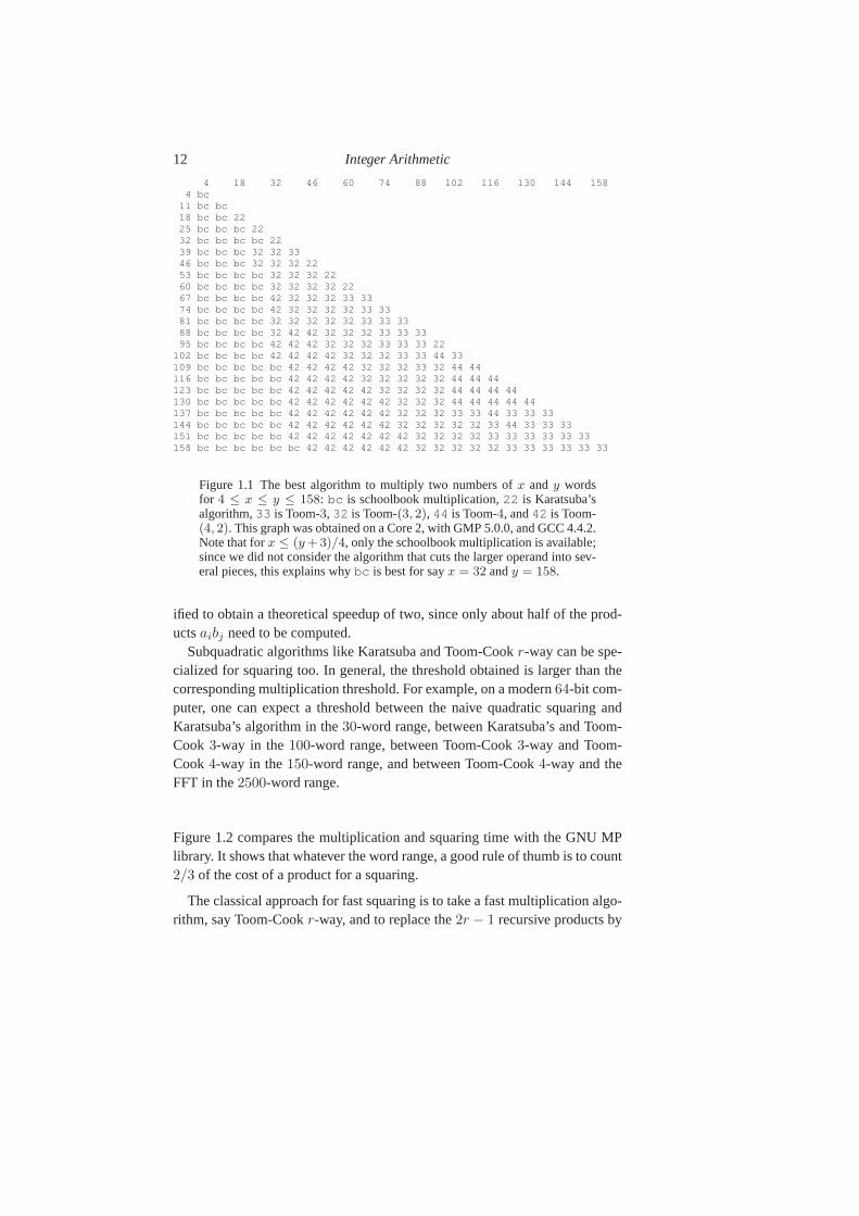
11 bc bc18 bc bc 2225 bc bc bc 2232 bc bc bc bc 2239 bc bc bc 32 32 3346 bc bc bc 32 32 32 2253 bc bc bc bc 32 32 32 2260 bc bc bc bc 32 32 32 32 2267 bc bc bc bc 42 32 32 32 33 3374 bc bc bc bc 42 32 32 32 32 33 3381 bc bc bc bc 32 32 32 32 32 33 33 3388 bc bc bc bc 32 42 42 32 32 32 33 33 3395 bc bc bc bc 42 42 42 32 32 32 33 33 33 22
102 bc bc bc bc 42 42 42 42 32 32 32 33 33 44 33109 bc bc bc bc bc 42 42 42 42 32 32 32 33 32 44 44116 bc bc bc bc bc 42 42 42 42 32 32 32 32 32 44 44 44123 bc bc bc bc bc 42 42 42 42 42 32 32 32 32 44 44 44 44130 bc bc bc bc bc 42 42 42 42 42 42 32 32 32 44 44 44 44 44137 bc bc bc bc bc 42 42 42 42 42 42 32 32 32 33 33 44 33 33 33144 bc bc bc bc bc 42 42 42 42 42 42 32 32 32 32 32 33 44 33 33 33151 bc bc bc bc bc 42 42 42 42 42 42 42 32 32 32 32 33 33 33 33 33 33158 bc bc bc bc bc bc 42 42 42 42 42 42 32 32 32 32 32 33 33 33 33 33 33
Figure 1.1 The best algorithm to multiply two numbers ofx andy wordsfor 4 ≤ x ≤ y ≤ 158: bc is schoolbook multiplication,22 is Karatsuba’salgorithm,33 is Toom-3, 32 is Toom-(3, 2), 44 is Toom-4, and42 is Toom-(4, 2). This graph was obtained on a Core 2, with GMP 5.0.0, and GCC 4.4.2.Note that forx ≤ (y +3)/4, only the schoolbook multiplication is available;since we did not consider the algorithm that cuts the larger operand into sev-eral pieces, this explains whybc is best for sayx = 32 andy = 158.
ified to obtain a theoretical speedup of two, since only abouthalf of the prod-uctsaibj need to be computed.
Subquadratic algorithms like Karatsuba and Toom-Cookr-way can be spe-cialized for squaring too. In general, the threshold obtained is larger than thecorresponding multiplication threshold. For example, on amodern64-bit com-puter, one can expect a threshold between the naive quadratic squaring andKaratsuba’s algorithm in the30-word range, between Karatsuba’s and Toom-Cook 3-way in the100-word range, between Toom-Cook3-way and Toom-Cook4-way in the150-word range, and between Toom-Cook4-way and theFFT in the2500-word range.
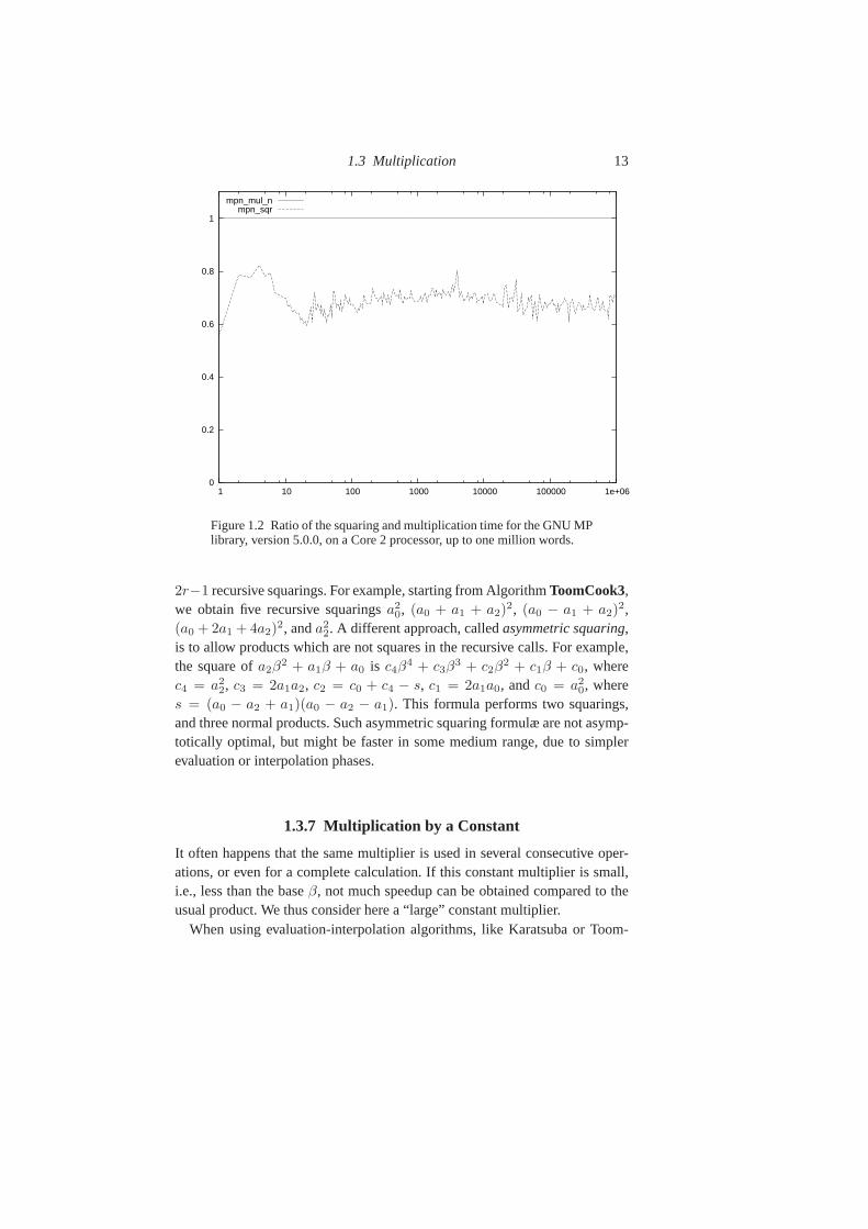
Figure 1.2 compares the multiplication and squaring time with the GNU MPlibrary. It shows that whatever the word range, a good rule ofthumb is to count2/3 of the cost of a product for a squaring.
The classical approach for fast squaring is to take a fast multiplication algo-rithm, say Toom-Cookr-way, and to replace the2r − 1 recursive products by
1.3 Multiplication 13
0
0.2
0.4
0.6
0.8
1
1 10 100 1000 10000 100000 1e+06
mpn_mul_nmpn_sqr
Figure 1.2 Ratio of the squaring and multiplication time for the GNU MPlibrary, version 5.0.0, on a Core 2 processor, up to one million words.
2r−1 recursive squarings. For example, starting from AlgorithmToomCook3,we obtain five recursive squaringsa2
0, (a0 + a1 + a2)2, (a0 − a1 + a2)
2,(a0 + 2a1 + 4a2)
2, anda22. A different approach, calledasymmetric squaring,
is to allow products which are not squares in the recursive calls. For example,the square ofa2β
2 + a1β + a0 is c4β4 + c3β
3 + c2β2 + c1β + c0, where
c4 = a22, c3 = 2a1a2, c2 = c0 + c4 − s, c1 = 2a1a0, andc0 = a2
0, wheres = (a0 − a2 + a1)(a0 − a2 − a1). This formula performs two squarings,and three normal products. Such asymmetric squaring formulæ are not asymp-totically optimal, but might be faster in some medium range,due to simplerevaluation or interpolation phases.
1.3.7 Multiplication by a Constant
It often happens that the same multiplier is used in several consecutive oper-ations, or even for a complete calculation. If this constantmultiplier is small,i.e., less than the baseβ, not much speedup can be obtained compared to theusual product. We thus consider here a “large” constant multiplier.
When using evaluation-interpolation algorithms, like Karatsuba or Toom-
14 Integer Arithmetic
Cook (see§1.3.2–1.3.3), one may store the evaluations for that fixed multiplierat the different points chosen.
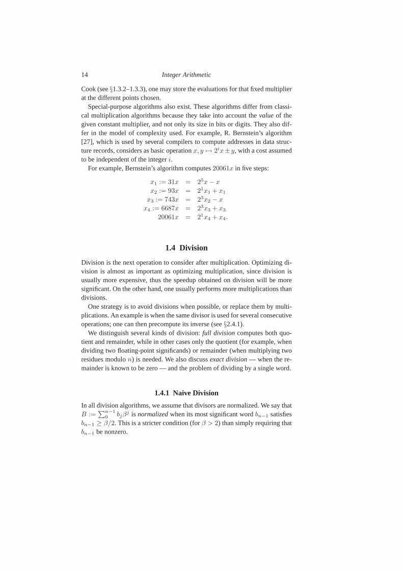
Special-purpose algorithms also exist. These algorithms differ from classi-cal multiplication algorithms because they take into account thevalueof thegiven constant multiplier, and not only its size in bits or digits. They also dif-fer in the model of complexity used. For example, R. Bernstein’s algorithm[27], which is used by several compilers to compute addresses in data struc-ture records, considers as basic operationx, y 7→ 2ix± y, with a cost assumedto be independent of the integeri.
For example, Bernstein’s algorithm computes20061x in five steps:
x1 := 31x = 25x − x
x2 := 93x = 21x1 + x1
x3 := 743x = 23x2 − x
x4 := 6687x = 23x3 + x3
20061x = 21x4 + x4.
1.4 Division
Division is the next operation to consider after multiplication. Optimizing di-vision is almost as important as optimizing multiplication, since division isusually more expensive, thus the speedup obtained on division will be moresignificant. On the other hand, one usually performs more multiplications thandivisions.
One strategy is to avoid divisions when possible, or replacethem by multi-plications. An example is when the same divisor is used for several consecutiveoperations; one can then precompute its inverse (see§2.4.1).
We distinguish several kinds of division:full division computes both quo-tient and remainder, while in other cases only the quotient (for example, whendividing two floating-point significands) or remainder (when multiplying tworesidues modulon) is needed. We also discussexact division— when the re-mainder is known to be zero — and the problem of dividing by a single word.
1.4.1 Naive Division
In all division algorithms, we assume that divisors are normalized. We say thatB :=
∑n−10 bjβ
j is normalizedwhen its most significant wordbn−1 satisfiesbn−1 ≥ β/2. This is a stricter condition (forβ > 2) than simply requiring thatbn−1 be nonzero.
1.4 Division 15
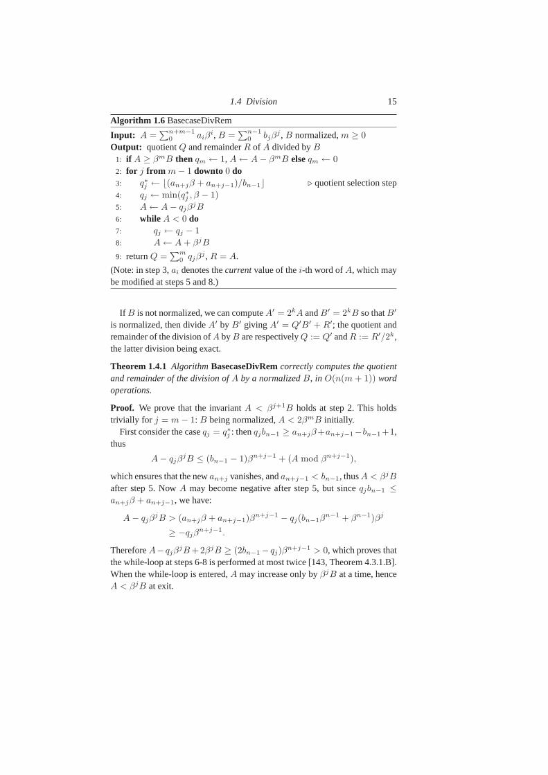
Algorithm 1.6 BasecaseDivRem
Input: A =∑n+m−1
0 aiβi, B =
∑n−10 bjβ
j , B normalized,m ≥ 0
Output: quotientQ and remainderR of A divided byB
1: if A ≥ βmB then qm ← 1, A ← A − βmB elseqm ← 0
2: for j from m − 1 downto 0 do3: q∗j ← ⌊(an+jβ + an+j−1)/bn−1⌋ ⊲ quotient selection step4: qj ← min(q∗j , β − 1)
5: A ← A − qjβjB
6: while A < 0 do7: qj ← qj − 1
8: A ← A + βjB
9: returnQ =∑m
0 qjβj , R = A.
(Note: in step 3,ai denotes thecurrentvalue of thei-th word ofA, which maybe modified at steps 5 and 8.)
If B is not normalized, we can computeA′ = 2kA andB′ = 2kB so thatB′
is normalized, then divideA′ by B′ giving A′ = Q′B′ + R′; the quotient andremainder of the division ofA byB are respectivelyQ := Q′ andR := R′/2k,the latter division being exact.
Theorem 1.4.1 AlgorithmBasecaseDivRemcorrectly computes the quotientand remainder of the division ofA by a normalizedB, in O(n(m + 1)) wordoperations.
Proof. We prove that the invariantA < βj+1B holds at step 2. This holdstrivially for j = m − 1: B being normalized,A < 2βmB initially.
First consider the caseqj = q∗j : thenqjbn−1 ≥ an+jβ+an+j−1−bn−1+1,thus
A − qjβjB ≤ (bn−1 − 1)βn+j−1 + (A mod βn+j−1),
which ensures that the newan+j vanishes, andan+j−1 < bn−1, thusA < βjB
after step 5. NowA may become negative after step 5, but sinceqjbn−1 ≤an+jβ + an+j−1, we have:
A − qjβjB > (an+jβ + an+j−1)β
n+j−1 − qj(bn−1βn−1 + βn−1)βj
≥ −qjβn+j−1.
ThereforeA− qjβjB +2βjB ≥ (2bn−1 − qj)β
n+j−1 > 0, which proves thatthe while-loop at steps 6-8 is performed at most twice [143, Theorem 4.3.1.B].When the while-loop is entered,A may increase only byβjB at a time, henceA < βjB at exit.
16 Integer Arithmetic
In the caseqj 6= q∗j , i.e., q∗j ≥ β, we have before the while-loop:A <
βj+1B − (β − 1)βjB = βjB, thus the invariant holds. If the while-loop isentered, the same reasoning as above holds.
We conclude that when the for-loop ends,0 ≤ A < B holds, and since(∑m
j qjβj)B + A is invariant throughout the algorithm, the quotientQ and
remainderR are correct.The most expensive part is step 5, which costsO(n) operations forqjB (the
multiplication byβj is simply a word-shift); the total cost isO(n(m + 1)).(Form = 0 we needO(n) work if A ≥ B, and even ifA < B to compare theinputs in the caseA = B − 1.)
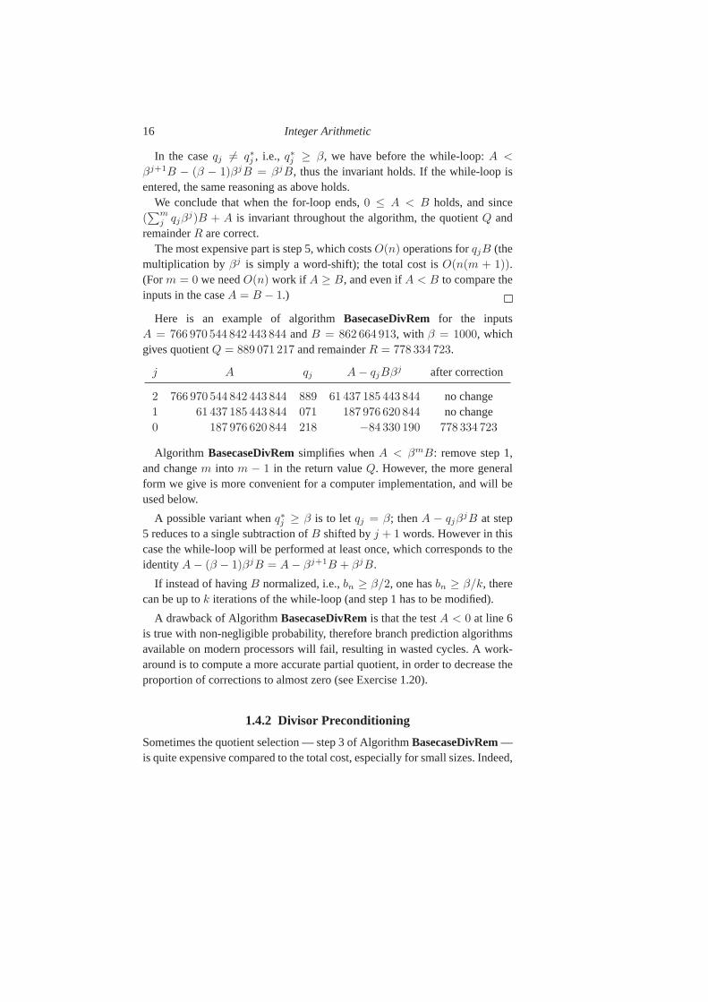
Here is an example of algorithmBasecaseDivRemfor the inputsA = 766 970 544 842 443 844 andB = 862 664 913, with β = 1000, whichgives quotientQ = 889 071 217 and remainderR = 778 334 723.
j A qj A − qjBβj after correction
2 766 970 544 842 443 844 889 61 437 185 443 844 no change1 61 437 185 443 844 071 187 976 620 844 no change0 187 976 620 844 218 −84 330 190 778 334 723
Algorithm BasecaseDivRemsimplifies whenA < βmB: remove step 1,and changem into m − 1 in the return valueQ. However, the more generalform we give is more convenient for a computer implementation, and will beused below.
A possible variant whenq∗j ≥ β is to let qj = β; thenA − qjβjB at step
5 reduces to a single subtraction ofB shifted byj + 1 words. However in thiscase the while-loop will be performed at least once, which corresponds to theidentityA − (β − 1)βjB = A − βj+1B + βjB.
If instead of havingB normalized, i.e.,bn ≥ β/2, one hasbn ≥ β/k, therecan be up tok iterations of the while-loop (and step 1 has to be modified).
A drawback of AlgorithmBasecaseDivRemis that the testA < 0 at line 6is true with non-negligible probability, therefore branchprediction algorithmsavailable on modern processors will fail, resulting in wasted cycles. A work-around is to compute a more accurate partial quotient, in order to decrease theproportion of corrections to almost zero (see Exercise 1.20).
1.4.2 Divisor Preconditioning
Sometimes the quotient selection — step 3 of AlgorithmBasecaseDivRem—is quite expensive compared to the total cost, especially for small sizes. Indeed,
1.4 Division 17
some processors do not have a machine instruction for the division of twowords by one word; one way to computeq∗j is then to precompute a one-wordapproximation of the inverse ofbn−1, and to multiply it byan+jβ + an+j−1.
Svoboda’s algorithm makes the quotient selection trivial,after precondition-ing the divisor. The main idea is that ifbn−1 equals the baseβ in AlgorithmBasecaseDivRem, then the quotient selection is easy, since it suffices to takeq∗j = an+j . (In addition,q∗j ≤ β − 1 is then always fulfilled, thus step 4 ofBasecaseDivRemcan be avoided, andq∗j replaced byqj .)
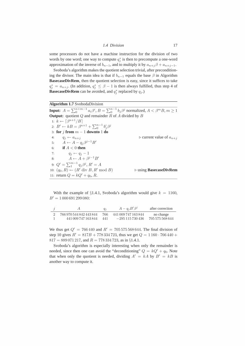
Algorithm 1.7 SvobodaDivision
Input: A =∑n+m−1
0 aiβi, B =
∑n−10 bjβ
j normalized,A < βmB, m ≥ 1
Output: quotientQ and remainderR of A divided byB
1: k ← ⌈βn+1/B⌉2: B′ ← kB = βn+1 +
∑n−10 b′jβ
j
3: for j from m − 1 downto 1 do4: qj ← an+j ⊲ current value ofan+j
5: A ← A − qjβj−1B′
6: if A < 0 then7: qj ← qj − 1
8: A ← A + βj−1B′
9: Q′ =∑m−1
1 qjβj , R′ = A
10: (q0, R) ← (R′ div B,R′ mod B) ⊲ usingBasecaseDivRem11: returnQ = kQ′ + q0, R.
With the example of§1.4.1, Svoboda’s algorithm would givek = 1160,B′ = 1000 691 299 080:
j A qj A − qjB′βj after correction
2 766 970 544 842 443 844 766 441 009 747 163 844 no change1 441 009 747 163 844 441 −295 115 730 436 705 575 568 644
We thus getQ′ = 766 440 andR′ = 705 575 568 644. The final division ofstep 10 givesR′ = 817B + 778 334 723, thus we getQ = 1160 · 766 440 +
817 = 889 071 217, andR = 778 334 723, as in§1.4.1.Svoboda’s algorithm is especially interesting when only the remainder is
needed, since then one can avoid the “deconditioning”Q = kQ′ + q0. Notethat when only the quotient is needed, dividingA′ = kA by B′ = kB isanother way to compute it.
18 Integer Arithmetic
1.4.3 Divide and Conquer Division
The base-case division of§1.4.1 determines the quotient word by word. Anatural idea is to try getting several words at a time, for example replacing thequotient selection step in AlgorithmBasecaseDivRemby:
q∗j ←⌊
an+jβ3 + an+j−1β
2 + an+j−2β + an+j−3
bn−1β + bn−2
⌋.
Sinceq∗j has then two words, fast multiplication algorithms (§1.3) might speedup the computation ofqjB at step 5 of AlgorithmBasecaseDivRem.
More generally, the most significant half of the quotient — say Q1, ofℓ = m − k words — mainly depends on theℓ most significant words of thedividend and divisor. Once a good approximation toQ1 is known, fast multi-plication algorithms can be used to compute the partial remainderA−Q1Bβk.The second idea of the divide and conquer algorithmRecursiveDivRemis tocompute the corresponding remainder together with the partial quotientQ1; insuch a way, one only has to subtract the product ofQ1 by the low part of thedivisor, before computing the low part of the quotient.
Algorithm 1.8 RecursiveDivRem
Input: A =∑n+m−1
0 aiβi, B =
∑n−10 bjβ
j , B normalized,n ≥ m
Output: quotientQ and remainderR of A divided byB
1: if m < 2 then returnBasecaseDivRem(A,B)
2: k ← ⌊m/2⌋, B1 ← B div βk, B0 ← B mod βk
3: (Q1, R1) ← RecursiveDivRem(A div β2k, B1)
4: A′ ← R1β2k + (A mod β2k) − Q1B0β
k
5: while A′ < 0 doQ1 ← Q1 − 1, A′ ← A′ + βkB
6: (Q0, R0) ← RecursiveDivRem(A′ div βk, B1)
7: A′′ ← R0βk + (A′ mod βk) − Q0B0
8: while A′′ < 0 doQ0 ← Q0 − 1, A′′ ← A′′ + B
9: returnQ := Q1βk + Q0, R := A′′.
In Algorithm RecursiveDivRem, one may replace the conditionm < 2 atstep 1 bym < T for any integerT ≥ 2. In practice,T is usually in the range50 to 200.
One can not requireA < βmB at input, since this condition may not besatisfied in the recursive calls. Consider for exampleA = 5517, B = 56 withβ = 10: the first recursive call will divide55 by 5, which yields a two-digitquotient11. EvenA ≤ βmB is not recursively fulfilled, as this example shows.The weakest possible input condition is that then most significant words ofA
1.4 Division 19
do not exceed those ofB, i.e.,A < βm(B + 1). In that case, the quotient isbounded byβm + ⌊(βm − 1)/B⌋, which yieldsβm + 1 in the casen = m
(compare Exercise 1.19). See also Exercise 1.22.
Theorem 1.4.2 Algorithm RecursiveDivRem is correct, and usesD(n +
m,n) operations, whereD(n+m,n) = 2D(n, n−m/2)+2M(m/2)+O(n).In particular D(n) := D(2n, n) satisfiesD(n) = 2D(n/2) + 2M(n/2) +
O(n), which givesD(n) ∼ M(n)/(2α−1 − 1) for M(n) ∼ nα, α > 1.
Proof. We first check the assumption for the recursive calls:B1 is normalizedsince it has the same most significant word thanB.
After step 3, we haveA = (Q1B1 + R1)β2k + (A mod β2k), thus after
step 4:A′ = A − Q1βkB, which still holds after step 5. After step 6, we have
A′ = (Q0B1 + R0)βk + (A′ mod βk), thus after step 7:A′′ = A′ − Q0B,
which still holds after step 8. At step 9 we thus haveA = QB + R.A div β2k hasm+n−2k words, whileB1 hasn−k words, thus0 ≤ Q1 <
2βm−k and0 ≤ R1 < B1 < βn−k. Thus at step 4,−2βm+k < A′ < βkB.SinceB is normalized, the while-loop at step 5 is performed at most four times(this can happen only whenn = m). At step 6 we have0 ≤ A′ < βkB, thusA′ div βk has at mostn words.
It follows 0 ≤ Q0 < 2βk and0 ≤ R0 < B1 < βn−k. Hence at step7, −2β2k < A′′ < B, and after at most four iterations at step 8, we have0 ≤ A′′ < B.
Theorem 1.4.2 givesD(n) ∼ 2M(n) for Karatsuba multiplication, andD(n) ∼ 2.63M(n) for Toom-Cook3-way; in the FFT range, see Exercise 1.23.
The same idea as in Exercise 1.20 applies: to decrease the probability thatthe estimated quotientsQ1 andQ0 are too large, use one extra word of thetruncated dividend and divisors in the recursive calls toRecursiveDivRem.
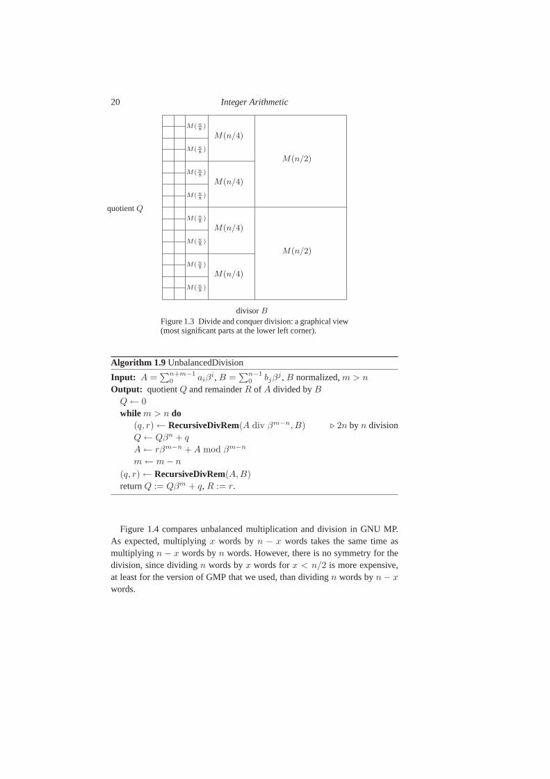
A graphical view of AlgorithmRecursiveDivRem in the casem = n isgiven in Figure 1.3, which represents the multiplicationQ · B: one first com-putes the lower left corner inD(n/2) (step 3), second the lower right cornerin M(n/2) (step 4), third the upper left corner inD(n/2) (step 6), and finallythe upper right corner inM(n/2) (step 7).
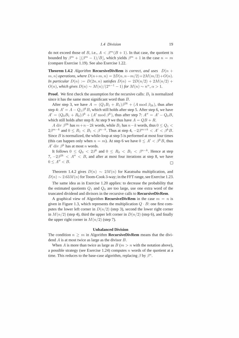
Unbalanced DivisionThe conditionn ≥ m in Algorithm RecursiveDivRemmeans that the divi-dendA is at most twice as large as the divisorB.
WhenA is more than twice as large asB (m > n with the notation above),a possible strategy (see Exercise 1.24) computesn words of the quotient at atime. This reduces to the base-case algorithm, replacingβ by βn.
20 Integer Arithmetic
quotientQ
divisorB
M(n/2)
M(n/2)
M(n/4)
M(n/4)
M(n/4)
M(n/4)
M( n8)
M( n8)
M( n8)
M( n8)
M( n8)
M( n8)
M( n8)
M( n8)
Figure 1.3 Divide and conquer division: a graphical view(most significant parts at the lower left corner).
Algorithm 1.9 UnbalancedDivision
Input: A =∑n+m−1
0 aiβi, B =
∑n−10 bjβ
j , B normalized,m > n
Output: quotientQ and remainderR of A divided byB
Q ← 0
while m > n do(q, r) ← RecursiveDivRem(A div βm−n, B) ⊲ 2n by n divisionQ ← Qβn + q
A ← rβm−n + A mod βm−n
m ← m − n
(q, r) ← RecursiveDivRem(A,B)
returnQ := Qβm + q, R := r.
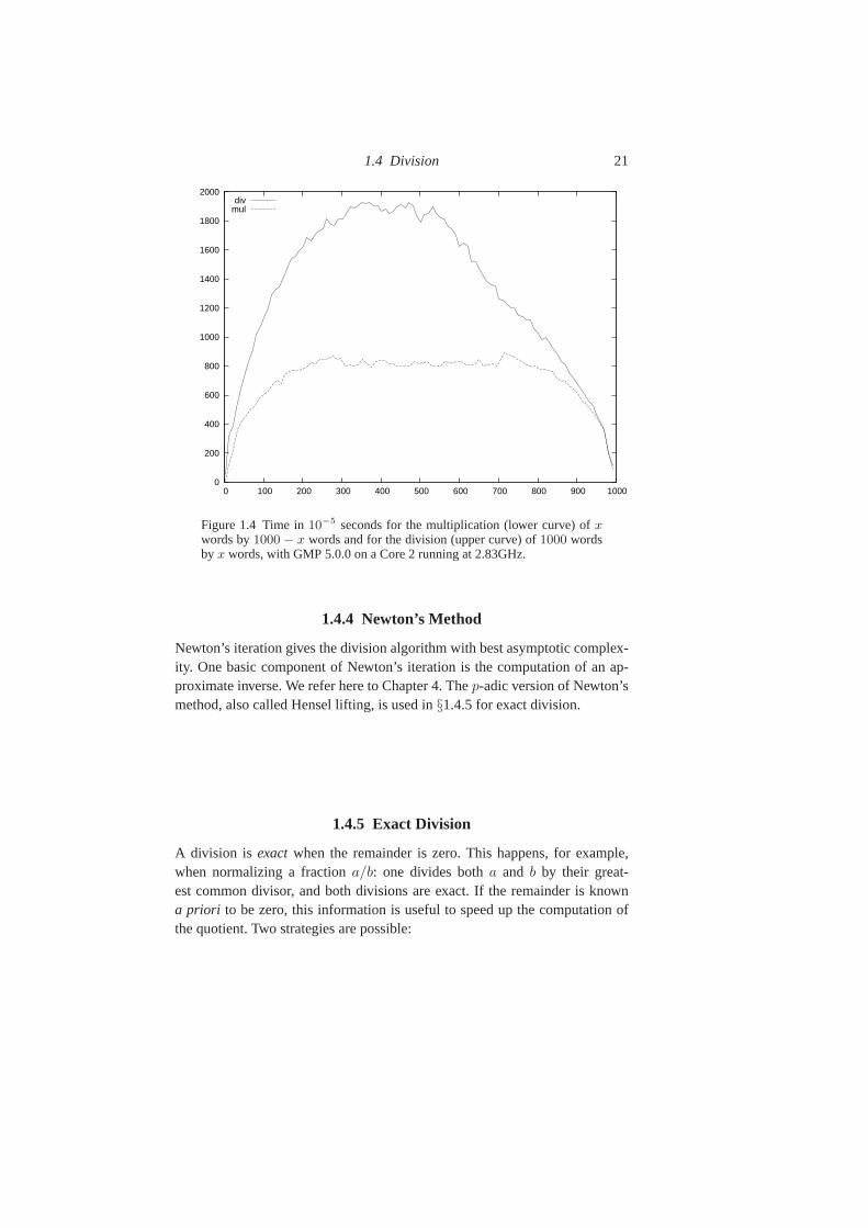
Figure 1.4 compares unbalanced multiplication and division in GNU MP.As expected, multiplyingx words byn − x words takes the same time asmultiplying n − x words byn words. However, there is no symmetry for thedivision, since dividingn words byx words forx < n/2 is more expensive,at least for the version of GMP that we used, than dividingn words byn − x
words.
1.4 Division 21
0
200
400
600
800
1000
1200
1400
1600
1800
2000
0 100 200 300 400 500 600 700 800 900 1000
divmul
Figure 1.4 Time in10−5 seconds for the multiplication (lower curve) ofxwords by1000 − x words and for the division (upper curve) of1000 wordsby x words, with GMP 5.0.0 on a Core 2 running at 2.83GHz.
1.4.4 Newton’s Method
Newton’s iteration gives the division algorithm with best asymptotic complex-ity. One basic component of Newton’s iteration is the computation of an ap-proximate inverse. We refer here to Chapter 4. Thep-adic version of Newton’smethod, also called Hensel lifting, is used in§1.4.5 for exact division.
1.4.5 Exact Division
A division is exactwhen the remainder is zero. This happens, for example,when normalizing a fractiona/b: one divides botha and b by their great-est common divisor, and both divisions are exact. If the remainder is knowna priori to be zero, this information is useful to speed up the computation ofthe quotient. Two strategies are possible:
22 Integer Arithmetic
• use MSB (most significant bits first) division algorithms, without computingthe lower part of the remainder. Here, one has to take care of rounding errors,in order to guarantee the correctness of the final result; or
• use LSB (least significant bits first) algorithms. If the quotient is known tobe less thanβn, computinga/b mod βn will reveal it.
Subquadratic algorithms can use both strategies. We describe a least significantbit algorithm using Hensel lifting, which can be viewed as ap-adic version ofNewton’s method:
Algorithm 1.10 ExactDivision
Input: A =∑n−1
0 aiβi, B =
∑n−10 bjβ
j
Output: quotientQ = A/B mod βn
Require: gcd(b0, β) = 1
1: C ← 1/b0 mod β
2: for i from ⌈lg n⌉ − 1 downto 1 do3: k ← ⌈n/2i⌉4: C ← C + C(1 − BC) mod βk
5: Q ← AC mod βk
6: Q ← Q + C(A − BQ) mod βn.
Algorithm ExactDivision uses the Karp-Markstein trick: lines 1-4 compute1/B mod β⌈n/2⌉, while the two last lines incorporate the dividend to obtainA/B mod βn. Note that themiddle product(§3.3.2) can be used in lines 4 and6, to speed up the computation of1 − BC andA − BQ respectively.
A further gain can be obtained by using both strategies simultaneously: com-pute the most significantn/2 bits of the quotient using the MSB strategy, andthe least significantn/2 bits using the LSB strategy. Since a division of sizen
is replaced by two divisions of sizen/2, this gives a speedup of up to two forquadratic algorithms (see Exercise 1.27).
1.4.6 Only Quotient or Remainder Wanted
When both the quotient and remainder of a division are needed,it is best tocompute them simultaneously. This may seem to be a trivial statement, nev-ertheless some high-level languages provide bothdiv andmod, but no singleinstruction to compute both quotient and remainder.
Once the quotient is known, the remainder can be recovered bya singlemultiplication asA − QB; on the other hand, when the remainder is known,the quotient can be recovered by an exact division as(A − R)/B (§1.4.5).
1.4 Division 23
However, it often happens that only one of the quotient or remainder isneeded. For example, the division of two floating-point numbers reduces to thequotient of their significands (see Chapter 3). Conversely,the multiplication oftwo numbers moduloN reduces to the remainder of their product after divi-sion byN (see Chapter 2). In such cases, one may wonder if faster algorithmsexist.
For a dividend of2n words and a divisor ofn words, a significant speedup— up to a factor of two for quadratic algorithms — can be obtained when onlythe quotient is needed, since one does not need to update the low n words ofthe current remainder (step 5 of AlgorithmBasecaseDivRem).
It seems difficult to get a similar speedup when only the remainder is re-quired. One possibility is to use Svoboda’s algorithm, but this requires someprecomputation, so is only useful when several divisions are performed withthe same divisor. The idea is the following: precompute a multiple B1 of B,having 3n/2 words, then/2 most significant words beingβn/2. Then re-ducing A mod B1 requires a singlen/2 × n multiplication. OnceA is re-duced toA1 of 3n/2 words by Svoboda’s algorithm with cost2M(n/2), useRecursiveDivRemon A1 andB, which costsD(n/2) + M(n/2). The to-tal cost is thus3M(n/2) + D(n/2), instead of2M(n/2) + 2D(n/2) for afull division with RecursiveDivRem. This gives5M(n)/3 for Karatsuba and2.04M(n) for Toom-Cook3-way, instead of2M(n) and2.63M(n) respec-tively. A similar algorithm is described in§2.4.2 (Subquadratic MontgomeryReduction) with further optimizations.
1.4.7 Division by a Single Word
We assume here that we want to divide a multiple precision number by a one-word integerc. As for multiplication by a one-word integer, this is an importantspecial case. It arises for example in Toom-Cook multiplication, where one hasto perform an exact division by3 (§1.3.3). One could of course use a classicaldivision algorithm (§1.4.1). Whengcd(c, β) = 1, Algorithm DivideByWordmight be used to compute a modular division:
A + bβn = cQ,
where the “carry”b will be zero when the division is exact.
Theorem 1.4.3 The output of Alg.DivideByWord satisfiesA + bβn = cQ.
Proof. We show that after stepi, 0 ≤ i < n, we haveAi+bβi+1 = cQi, whereAi :=
∑ij=0 aiβ
i andQi :=∑i
j=0 qiβi. For i = 0, this isa0 + bβ = cq0,
which is just line 7: sinceq0 = a0/c mod β, q0c−a0 is divisible byβ. Assume
24 Integer Arithmetic
Algorithm 1.11 DivideByWord
Input: A =∑n−1
0 aiβi, 0 ≤ c < β, gcd(c, β) = 1
Output: Q =∑n−1
0 qiβi and0 ≤ b < c such thatA + bβn = cQ
1: d ← 1/c mod β ⊲ might be precomputed2: b ← 0
3: for i from 0 to n − 1 do4: if b ≤ ai then (x, b′) ← (ai − b, 0)
5: else(x, b′) ← (ai − b + β, 1)
6: qi ← dx mod β
7: b′′ ← (qic − x)/β
8: b ← b′ + b′′
9: return∑n−1
0 qiβi, b.
now thatAi−1 + bβi = cQi−1 holds for1 ≤ i < n. We haveai − b+ b′β = x,sox + b′′β = cqi, thusAi + (b′ + b′′)βi+1 = Ai−1 + βi(ai + b′β + b′′β) =
cQi−1 − bβi + βi(x + b− b′β + b′β + b′′β) = cQi−1 + βi(x + b′′β) = cQi.
REMARK : at step 7, since0 ≤ x < β, b′′ can also be obtained as⌊qic/β⌋.Algorithm DivideByWord is just a special case of Hensel’s division, which
is the topic of the next section; it can easily be extended to divide by integersof a few words.
1.4.8 Hensel’s Division
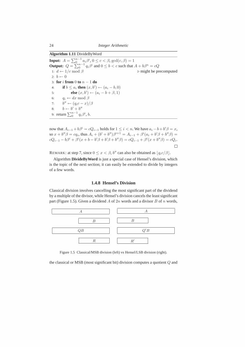
Classical division involves cancelling the most significant part of the dividendby a multiple of the divisor, while Hensel’s division cancels the least significantpart (Figure 1.5). Given a dividendA of 2n words and a divisorB of n words,
A
B
QB
R
A
B
Q′B
R′
Figure 1.5 Classical/MSB division (left) vs Hensel/LSB division (right).
the classical or MSB (most significant bit) division computes a quotientQ and
1.5 Roots 25
a remainderR such thatA = QB+R, while Hensel’s or LSB (least significantbit) division computes a LSB-quotientQ′ and a LSB-remainderR′ such thatA = Q′B + R′βn. While MSB division requires the most significant bit ofB
to be set, LSB division requiresB to be relatively prime to the word baseβ,i.e.,B to be odd forβ a power of two.
The LSB-quotient is uniquely defined byQ′ = A/B mod βn, with0 ≤ Q′ < βn. This in turn uniquely defines the LSB-remainderR′ =
(A − Q′B)β−n, with −B < R′ < βn.
Most MSB-division variants (naive, with preconditioning,divide and con-quer, Newton’s iteration) have their LSB-counterpart. Forexample, LSB pre-conditioning involves using a multiplekB of the divisor such thatkB =
1 mod β, and Newton’s iteration is called Hensel lifting in the LSB case. Theexact division algorithm described at the end of§1.4.5 uses both MSB- andLSB-division simultaneously. One important difference isthat LSB-divisiondoes not need any correction step, since the carries go in thedirection oppositeto the cancelled bits.
When only the remainder is wanted, Hensel’s division is usually known asMontgomery reduction (see§2.4.2).
1.5 Roots
1.5.1 Square Root
The “paper and pencil” method once taught at school to extract square roots isvery similar to “paper and pencil” division. It decomposes an integerm of theform s2 + r, taking two digits ofm at a time, and finding one digit ofs foreach two digits ofm. It is based on the following idea. Ifm = s2 + r is thecurrent decomposition, then taking two more digits of the argument, we have adecomposition of the form100m+r′ = 100s2 +100r+r′ with 0 ≤ r′ < 100.Since(10s + t)2 = 100s2 + 20st + t2, a good approximation to the next digitt can be found by dividing10r by 2s.
Algorithm SqrtRem generalizes this idea to a powerβℓ of the internal baseclose tom1/4: one obtains a divide and conquer algorithm, which is in factanerror-free variant of Newton’s method (cf Chapter 4):
26 Integer Arithmetic
Algorithm 1.12 SqrtRem
Input: m = an−1βn−1 + · · · + a1β + a0 with an−1 6= 0
Output: (s, r) such thats2 ≤ m = s2 + r < (s + 1)2
Require: a base-case routineBasecaseSqrtRemℓ ← ⌊(n − 1)/4⌋if ℓ = 0 then returnBasecaseSqrtRem(m)
write m = a3β3ℓ + a2β
2ℓ + a1βℓ + a0 with 0 ≤ a2, a1, a0 < βℓ
(s′, r′) ← SqrtRem(a3βℓ + a2)
(q, u) ← DivRem(r′βℓ + a1, 2s′)s ← s′βℓ + q
r ← uβℓ + a0 − q2
if r < 0 thenr ← r + 2s − 1, s ← s − 1
return(s, r).
Theorem 1.5.1 AlgorithmSqrtRem correctly returns the integer square roots and remainderr of the inputm, and has complexityR(2n) ∼ R(n) +
D(n) + S(n) whereD(n) andS(n) are the complexities of the division withremainder and squaring respectively. This givesR(n) ∼ n2/2 with naivemultiplication,R(n) ∼ 4K(n)/3 with Karatsuba’s multiplication, assumingS(n) ∼ 2M(n)/3.
As an example, assume AlgorithmSqrtRem is called onm = 123 456 789
with β = 10. One hasn = 9, ℓ = 2, a3 = 123, a2 = 45, a1 = 67, anda0 = 89. The recursive call fora3β
ℓ + a2 = 12 345 yields s′ = 111 andr′ = 24. TheDivRem call yieldsq = 11 andu = 25, which givess = 11 111
andr = 2468.
Another nice way to compute the integer square root of an integerm, i.e.,⌊m1/2⌋, is Algorithm SqrtInt , which is an all-integer version of Newton’smethod (§4.2).
Still with input123 456 789, we successively gets = 61 728 395, 30 864 198,15 432 100, 7 716 053, 3 858 034, 1 929 032, 964 547, 482 337, 241 296,120 903, 60 962, 31 493, 17 706, 12 339, 11 172, 11 111, 11 111. Convergenceis slow because the initial value ofu assigned at line 1 is much too large. How-ever, any initial value greater than or equal to⌊m1/2⌋ works (see the proof ofAlgorithm RootInt below): starting froms = 12 000, one getss = 11 144
thens = 11 111. See Exercise 1.28.
1.5 Roots 27
Algorithm 1.13 SqrtIntInput: an integerm ≥ 1
Output: s = ⌊m1/2⌋1: u ← m ⊲ any valueu ≥ ⌊m1/2⌋ works2: repeat3: s ← u
4: t ← s + ⌊m/s⌋5: u ← ⌊t/2⌋6: until u ≥ s
7: returns.
1.5.2 k-th Root
The idea of AlgorithmSqrtRem for the integer square root can be generalizedto any power: if the current decomposition ism = m′βk + m′′βk−1 + m′′′,first compute ak-th root of m′, saym′ = sk + r, then dividerβ + m′′ byksk−1 to get an approximation of the next root digitt, and correct it if needed.Unfortunately the computation of the remainder, which is easy for the squareroot, involvesO(k) terms for thek-th root, and this method may be slowerthan Newton’s method with floating-point arithmetic (§4.2.3).
Similarly, AlgorithmSqrtInt can be generalized to thek-th root (see Algo-rithm RootInt ).
Algorithm 1.14 RootIntInput: integersm ≥ 1, andk ≥ 2
Output: s = ⌊m1/k⌋1: u ← m ⊲ any valueu ≥ ⌊m1/k⌋ works2: repeat3: s ← u
4: t ← (k − 1)s + ⌊m/sk−1⌋5: u ← ⌊t/k⌋6: until u ≥ s
7: returns.
Theorem 1.5.2 AlgorithmRootInt terminates and returns⌊m1/k⌋.
Proof. As long asu < s in step 6, the sequence ofs-values is decreasing,thus it suffices to consider what happens whenu ≥ s. First it is easy so seethatu ≥ s impliesm ≥ sk, becauset ≥ ks thus(k − 1)s + m/sk−1 ≥ ks.
28 Integer Arithmetic
Consider now the functionf(t) := [(k − 1)t + m/tk−1]/k for t > 0; itsderivative is negative fort < m1/k, and positive fort > m1/k, thusf(t) ≥f(m1/k) = m1/k. This proves thats ≥ ⌊m1/k⌋. Together withs ≤ m1/k, thisproves thats = ⌊m1/k⌋ at the end of the algorithm.
Note that any initial value greater than or equal to⌊m1/k⌋ works at step 1.Incidentally, we have proved the correctness of AlgorithmSqrtInt , which isjust the special casek = 2 of Algorithm RootInt .
1.5.3 Exact Root
When ak-th root is known to be exact, there is of course no need to com-pute exactly the final remainder in “exact root” algorithms,which saves somecomputation time. However, one has to check that the remainder is sufficientlysmall that the computed root is correct.
When a root is known to be exact, one may also try to compute it startingfrom the least significant bits, as for exact division. Indeed, if sk = m, thensk = m mod βℓ for any integerℓ. However, in the case of exact division, theequationa = qb mod βℓ has only one solutionq as soon asb is relativelyprime toβ. Here, the equationsk = m mod βℓ may have several solutions,so the lifting process is not unique. For example,x2 = 1 mod 23 has foursolutions1, 3, 5, 7.
Suppose we havesk = m mod βℓ, and we want to lift toβℓ+1. This implies(s + tβℓ)k = m + m′βℓ mod βℓ+1 where0 ≤ t,m′ < β. Thus
kt = m′ +m − sk
βℓmod β.
This equation has a unique solutiont when k is relatively prime toβ. Forexample, we can extract cube roots in this way forβ a power of two. Whenkis relatively prime toβ, we can also compute the root simultaneously from themost significant and least significant ends, as for exact division.
Unknown ExponentAssume now that one wants to check if a given integerm is an exact power,without knowing the corresponding exponent. For example, some primalitytesting or factorization algorithms fail when given an exact power, so this hasto be checked first. AlgorithmIsPower detects exact powers, and returns thelargest corresponding exponent (or1 if the input is not an exact power).
To quickly detect non-k-th powers at step 2, one may use modular algo-rithms whenk is relatively prime to the baseβ (see above).REMARK : in Algorithm IsPower, one can limit the search to prime exponents
1.6 Greatest Common Divisor 29
Algorithm 1.15 IsPowerInput: a positive integermOutput: k ≥ 2 whenm is an exactk-th power,1 otherwise
1: for k from ⌊lg m⌋ downto 2 do2: if m is ak-th powerthen returnk
3: return1.
k, but then the algorithm does not necessarily return the largest exponent, andwe might have to call it again. For example, takingm = 117649, the modifiedalgorithm first returns3 because117649 = 493, and when called again withm = 49 it returns2.
1.6 Greatest Common Divisor
Many algorithms for computing gcds may be found in the literature. We candistinguish between the following (non-exclusive) types:
• left-to-right (MSB) versus right-to-left (LSB) algorithms: in the former theactions depend on the most significant bits, while in the latter the actionsdepend on the least significant bits;
• naive algorithms: theseO(n2) algorithms consider one word of each operandat a time, trying to guess from them the first quotients; we count in this classalgorithms considering double-size words, namely Lehmer’s algorithm andSorenson’sk-ary reduction in the left-to-right and right-to-left cases respec-tively; algorithms not in this class consider a number of words that dependson the input sizen, and are often subquadratic;
• subtraction-only algorithms: these algorithms trade divisions for subtrac-tions, at the cost of more iterations;
• plain versus extended algorithms: the former just compute the gcd of theinputs, while the latter express the gcd as a linear combination of the inputs.
1.6.1 Naive GCD
For completeness we mention Euclid’s algorithm for finding the gcd of twonon-negative integersu, v.
Euclid’s algorithm is discussed in many textbooks, and we donot recom-mend it in its simplest form, except for testing purposes. Indeed, it is usually a
30 Integer Arithmetic
Algorithm 1.16 EuclidGcdInput: u, v nonnegative integers (not both zero)Output: gcd(u, v)
while v 6= 0 do(u, v) ← (v, u mod v)
returnu.
slow way to compute a gcd. However, Euclid’s algorithm does show the con-nection between gcds and continued fractions. Ifu/v has a regular continuedfraction of the form
u/v = q0 +1
q1+
1
q2+
1
q3+· · · ,
then the quotientsq0, q1, . . . are precisely the quotientsu div v of the divisionsperformed in Euclid’s algorithm. For more on continued fractions, see§4.6.
Double-Digit Gcd. A first improvement comes from Lehmer’s observation:the first few quotients in Euclid’s algorithm usually can be determined fromthe most significant words of the inputs. This avoids expensive divisions thatgive small quotients most of the time (see [143,§4.5.3]). Consider for exam-ple a = 427 419 669 081 andb = 321 110 693 270 with 3-digit words. Thefirst quotients are1, 3, 48, . . . Now if we consider the most significant words,namely427 and 321, we get the quotients1, 3, 35, . . .. If we stop after thefirst two quotients, we see that we can replace the initial inputs bya − b and−3a + 4b, which gives106 308 975 811 and2 183 765 837.
Lehmer’s algorithm determines cofactors from the most significant wordsof the input integers. Those cofactors usually have size only half a word. TheDoubleDigitGcd algorithm — which should be called “double-word” — usesthe two most significant words instead, which gives cofactorst, u, v, w of onefull-word each, such thatgcd(a, b) = gcd(ta+ub, va+wb). This is optimal forthe computation of the four productsta, ub, va, wb. With the above example,if we consider427 419 and321 110, we find that the first five quotients agree,so we can replacea, b by −148a + 197b and441a − 587b, i.e.,695 550 202
and97 115 231.The subroutineHalfBezout takes as input two2-word integers, performs
Euclid’s algorithm until the smallest remainder fits in one word, and returnsthe corresponding matrix[t, u; v, w].
Binary Gcd. A better algorithm than Euclid’s, though also ofO(n2) com-plexity, is thebinaryalgorithm. It differs from Euclid’s algorithm in two ways:
1.6 Greatest Common Divisor 31
Algorithm 1.17 DoubleDigitGcd
Input: a := an−1βn−1 + · · · + a0, b := bm−1β
m−1 + · · · + b0
Output: gcd(a, b)
if b = 0 then returna
if m < 2 then returnBasecaseGcd(a, b)
if a < b or n > m then returnDoubleDigitGcd(b, a mod b)
(t, u, v, w) ← HalfBezout(an−1β + an−2, bn−1β + bn−2)
returnDoubleDigitGcd(|ta + ub|, |va + wb|).
it consider least significant bits first, and it avoids divisions, except for divi-sions by two (which can be implemented as shifts on a binary computer). SeeAlgorithm BinaryGcd. Note that the first three “while” loops can be omittedif the inputsa andb are odd.
Algorithm 1.18 BinaryGcdInput: a, b > 0
Output: gcd(a, b)
t ← 1
while a mod 2 = b mod 2 = 0 do(t, a, b) ← (2t, a/2, b/2)
while a mod 2 = 0 doa ← a/2
while b mod 2 = 0 dob ← b/2 ⊲ nowa andb are both odd
while a 6= b do(a, b) ← (|a − b|,min(a, b))
a ← a/2ν(a) ⊲ ν(a) is the2-valuation ofa
returnta.
Sorenson’sk-ary reductionThe binary algorithm is based on the fact that ifa andb are both odd, thena−b
is even, and we can remove a factor of two sincegcd(a, b) is odd. Sorenson’sk-ary reduction is a generalization of that idea: givena andb odd, we try tofind small integersu, v such thatua− vb is divisible by a large power of two.
Theorem 1.6.1 [227] If a, b > 0, m > 1 with gcd(a,m) = gcd(b,m) = 1,there existu, v, 0 < |u|, v <
√m such thatua = vb mod m.
32 Integer Arithmetic
Algorithm ReducedRatModfinds such a pair(u, v); it is a simple variation ofthe extended Euclidean algorithm; indeed, theui are quotients in the continuedfraction expansion ofc/m.
Algorithm 1.19 ReducedRatModInput: a, b > 0, m > 1 with gcd(a,m) = gcd(b,m) = 1
Output: (u, v) such that0 < |u|, v <√
m andua = vb mod m
1: c ← a/b mod m
2: (u1, v1) ← (0,m)
3: (u2, v2) ← (1, c)
4: while v2 ≥ √m do
5: q ← ⌊v1/v2⌋6: (u1, u2) ← (u2, u1 − qu2)
7: (v1, v2) ← (v2, v1 − qv2)
8: return(u2, v2).
Whenm is a prime power, the inversion1/b mod m at step 1 of AlgorithmReducedRatModcan be performed efficiently using Hensel lifting (§2.5).
Given two integersa, b of sayn words, AlgorithmReducedRatModwithm = β2 returns two integersu, v such thatvb − ua is a multiple ofβ2. Sinceu, v have at most one word each,a′ = (vb−ua)/β2 has at mostn−1 words —plus possibly one bit — therefore withb′ = b mod a′ we obtaingcd(a, b) =
gcd(a′, b′), where botha′ andb′ have about one word less thanmax(a, b). Thisgives an LSB variant of the double-digit (MSB) algorithm.
1.6.2 Extended GCD
Algorithm ExtendedGcdsolves theextendedgreatest common divisor prob-lem: given two integersa andb, it computes their gcdg, and also two integersu andv (calledBezout coefficientsor sometimescofactorsor multipliers) suchthatg = ua + vb.
If a0 andb0 are the input numbers, anda, b the current values, the followinginvariants hold at the start of each iteration of the while loop and after the whileloop: a = ua0 + vb0, andb = wa0 + xb0. (See Exercise 1.30 for a bound onthe cofactoru.)
An important special case is modular inversion (see Chapter2): given anintegern, one wants to compute1/a mod n for a relatively prime ton. Onethen simply runs AlgorithmExtendedGcdwith inputa andb = n: this yields
1.6 Greatest Common Divisor 33
Algorithm 1.20 ExtendedGcdInput: positive integersa andb
Output: integers(g, u, v) such thatg = gcd(a, b) = ua + vb
1: (u,w) ← (1, 0)
2: (v, x) ← (0, 1)
3: while b 6= 0 do4: (q, r) ← DivRem(a, b)
5: (a, b) ← (b, r)
6: (u,w) ← (w, u − qw)
7: (v, x) ← (x, v − qx)
8: return(a, u, v).
u andv with ua + vn = 1, thus1/a = u mod n. Sincev is not needed here,we can simply avoid computingv andx, by removing steps 2 and 7.
It may also be worthwhile to compute onlyu in the general case, as thecofactorv can be recovered fromv = (g − ua)/b, this division being exact(see§1.4.5).
All known algorithms for subquadratic gcd rely on an extended gcd subrou-tine which is called recursively, so we discuss the subquadratic extended gcdin the next section.
1.6.3 Half Binary GCD, Divide and Conquer GCD
Designing a subquadratic integer gcd algorithm that is bothmathematicallycorrect and efficient in practice is a challenging problem.
A first remark is that, starting fromn-bit inputs, there areO(n) terms in theremainder sequencer0 = a, r1 = b, . . . ,ri+1 = ri−1 mod ri, . . . , and the sizeof ri decreases linearly withi. Thus, computing all the partial remaindersri
leads to a quadratic cost, and a fast algorithm should avoid this.However, the partial quotientsqi = ri−1 div ri are usually small: the main
idea is thus to compute them without computing the partial remainders. Thiscan be seen as a generalization of theDoubleDigitGcd algorithm: instead ofconsidering a fixed baseβ, adjust it so that the inputs have four “big words”.The cofactor-matrix returned by theHalfBezout subroutine will then reducethe input size to about3n/4. A second call with the remaining two most sig-nificant “big words” of the new remainders will reduce their size to half theinput size. See Exercise 1.31.
The same method applies in the LSB case, and is in fact simplerto turninto a correct algorithm. In this case, the termsri form a binary remainder
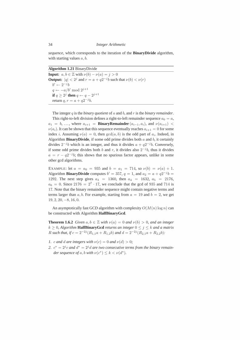
34 Integer Arithmetic
sequence, which corresponds to the iteration of theBinaryDivide algorithm,with starting valuesa, b.
Algorithm 1.21 BinaryDivide
Input: a, b ∈ Z with ν(b) − ν(a) = j > 0
Output: |q| < 2j andr = a + q2−jb such thatν(b) < ν(r)
b′ ← 2−jb
q ← −a/b′ mod 2j+1
if q ≥ 2j then q ← q − 2j+1
returnq, r = a + q2−jb.
The integerq is thebinary quotientof a andb, andr is thebinary remainder.This right-to-left division defines a right-to-left remainder sequencea0 = a,
a1 = b, . . . , whereai+1 = BinaryRemainder (ai−1, ai), andν(ai+1) <
ν(ai). It can be shown that this sequence eventually reachesai+1 = 0 for someindex i. Assumingν(a) = 0, thengcd(a, b) is the odd part ofai. Indeed, inAlgorithm BinaryDivide , if some odd prime divides botha andb, it certainlydivides2−jb which is an integer, and thus it dividesa + q2−jb. Conversely,if some odd prime divides bothb andr, it divides also2−jb, thus it dividesa = r − q2−jb; this shows that no spurious factor appears, unlike in someother gcd algorithms.
EXAMPLE : let a = a0 = 935 and b = a1 = 714, so ν(b) = ν(a) + 1.Algorithm BinaryDivide computesb′ = 357, q = 1, anda2 = a + q2−jb =
1292. The next step givesa3 = 1360, then a4 = 1632, a5 = 2176,a6 = 0. Since2176 = 27 · 17, we conclude that the gcd of935 and714 is17. Note that the binary remainder sequence might contain negative terms andterms larger thana, b. For example, starting froma = 19 andb = 2, we get19, 2, 20,−8, 16, 0.
An asymptotically fast GCD algorithm with complexityO(M(n) log n) canbe constructed with AlgorithmHalfBinaryGcd .
Theorem 1.6.2 Givena, b ∈ Z with ν(a) = 0 andν(b) > 0, and an integerk ≥ 0, AlgorithmHalfBinaryGcd returns an integer0 ≤ j ≤ k and a matrixR such that, ifc = 2−2j(R1,1a + R1,2b) andd = 2−2j(R2,1a + R2,2b):
1. c andd are integers withν(c) = 0 andν(d) > 0;
2. c∗ = 2jc andd∗ = 2jd are two consecutive terms from the binary remain-der sequence ofa, b with ν(c∗) ≤ k < ν(d∗).
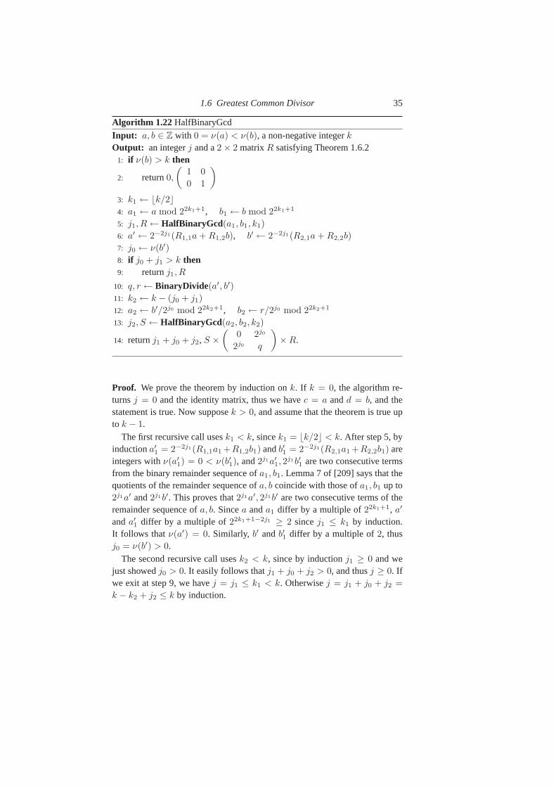
1.6 Greatest Common Divisor 35
Algorithm 1.22 HalfBinaryGcd
Input: a, b ∈ Z with 0 = ν(a) < ν(b), a non-negative integerkOutput: an integerj and a2 × 2 matrixR satisfying Theorem 1.6.2
1: if ν(b) > k then
2: return0,
(1 0
0 1
)
3: k1 ← ⌊k/2⌋4: a1 ← a mod 22k1+1, b1 ← b mod 22k1+1
5: j1, R ← HalfBinaryGcd (a1, b1, k1)
6: a′ ← 2−2j1(R1,1a + R1,2b), b′ ← 2−2j1(R2,1a + R2,2b)
7: j0 ← ν(b′)8: if j0 + j1 > k then9: returnj1, R
10: q, r ← BinaryDivide(a′, b′)11: k2 ← k − (j0 + j1)
12: a2 ← b′/2j0 mod 22k2+1, b2 ← r/2j0 mod 22k2+1
13: j2, S ← HalfBinaryGcd (a2, b2, k2)
14: returnj1 + j0 + j2, S ×(
0 2j0
2j0 q
)× R.
Proof. We prove the theorem by induction onk. If k = 0, the algorithm re-turnsj = 0 and the identity matrix, thus we havec = a andd = b, and thestatement is true. Now supposek > 0, and assume that the theorem is true upto k − 1.
The first recursive call usesk1 < k, sincek1 = ⌊k/2⌋ < k. After step 5, byinductiona′
1 = 2−2j1(R1,1a1 +R1,2b1) andb′1 = 2−2j1(R2,1a1 +R2,2b1) areintegers withν(a′
1) = 0 < ν(b′1), and2j1a′1, 2
j1b′1 are two consecutive termsfrom the binary remainder sequence ofa1, b1. Lemma 7 of [209] says that thequotients of the remainder sequence ofa, b coincide with those ofa1, b1 up to2j1a′ and2j1b′. This proves that2j1a′, 2j1b′ are two consecutive terms of theremainder sequence ofa, b. Sincea anda1 differ by a multiple of22k1+1, a′
anda′1 differ by a multiple of22k1+1−2j1 ≥ 2 sincej1 ≤ k1 by induction.
It follows that ν(a′) = 0. Similarly, b′ andb′1 differ by a multiple of2, thusj0 = ν(b′) > 0.
The second recursive call usesk2 < k, since by inductionj1 ≥ 0 and wejust showedj0 > 0. It easily follows thatj1 + j0 + j2 > 0, and thusj ≥ 0. Ifwe exit at step 9, we havej = j1 ≤ k1 < k. Otherwisej = j1 + j0 + j2 =
k − k2 + j2 ≤ k by induction.
36 Integer Arithmetic
If j0 + j1 > k, we haveν(2j1b′) = j0 + j1 > k, we exit the algorithm andthe statement holds. Now assumej0 + j1 ≤ k. We compute an extra termrof the remainder sequence froma′, b′, which up to multiplication by2j1 , is anextra term of the remainder sequence ofa, b. Sincer = a′ + q2−j0b′, we have
(b′
r
)= 2−j0
(0 2j0
2j0 q
)(a′
b′
).
The new terms of the remainder sequence areb′/2j0 andr/2j0 , adjusted so thatν(b′/2j0) = 0. The same argument as above holds for the second recursivecall, which stops when the2-valuation of the sequence starting froma2, b2
exceedsk2; this corresponds to a2-valuation larger thanj0 + j1 + k2 = k forthea, b remainder sequence.
Given twon-bit integersa andb, andk = n/2, HalfBinaryGcd yields twoconsecutive elementsc∗, d∗ of their binary remainder sequence with bit-sizeaboutn/2 (for their odd part).EXAMPLE : let a = 1889 826 700 059 andb = 421 872 857 844, with k = 20.The first recursive call witha1 = 1243 931, b1 = 1372 916, k1 = 10 givesj1 = 8 andR =
„
352 280260 393
«
, which corresponds toa′ = 11 952 871 683
and b′ = 10 027 328 112, with j0 = 4. The binary division yields the newterm r = 8819 331 648, and we havek2 = 8, a2 = 52 775, b2 = 50 468.The second recursive call givesj2 = 8 andS =
„
64 272212 −123
«
, which finally
givesj = 20 and the matrix„
1 444 544 1 086 512349 084 1 023 711
«
, which corresponds to the
remainder termsr8 = 2899 749 · 2j , r9 = 992 790 · 2j . With the samea, b
values, but withk = 41, which corresponds to the bit-size ofa, we get asfinal values of the algorithmr15 = 3 · 241 andr16 = 0, which proves thatgcd(a, b) = 3.
Let H(n) be the complexity ofHalfBinaryGcd for inputs of n bits andk = n/2; a1 andb1 have∼n/2 bits, the coefficients ofR have∼n/4 bits, anda′, b′ have∼3n/4 bits. The remaindersa2, b2 have∼n/2 bits, the coefficientsof S have∼n/4 bits, and the final valuesc, d have∼n/2 bits. The main costsare the matrix-vector product at step 6, and the final matrix-matrix product.We obtainH(n) ∼ 2H(n/2) + 4M(n/4, n) + 7M(n/4), assuming we useStrassen’s algorithm to multiply two2×2 matrices with7 scalar products, i.e.,H(n) ∼ 2H(n/2) + 17M(n/4), assuming that we compute eachM(n/4, n)
product with a single FFT transform of width5n/4, which gives cost aboutM(5n/8) ∼ 0.625M(n) in the FFT range. ThusH(n) = O(M(n) log n).
For the plain gcd, we callHalfBinaryGcd with k = n, and instead of com-puting the final matrix product, we multiply2−2j2S by (b′, r) — the com-
1.7 Base Conversion 37
ponents have∼n/2 bits — to obtain the finalc, d values. The first recur-sive call hasa1, b1 of sizen with k1 ≈ n/2, and corresponds toH(n); thematrix R anda′, b′ haven/2 bits, andk2 ≈ n/2, thus the second recursivecall corresponds to a plain gcd of sizen/2. The costG(n) satisfiesG(n) =
H(n)+G(n/2)+4M(n/2, n)+4M(n/2) ∼ H(n)+G(n/2)+10M(n/2).ThusG(n) = O(M(n) log n).
An application of the half gcdper sein the MSB case is therational recon-structionproblem. Assume one wants to compute a rationalp/q wherep andq
are known to be bounded by some constantc. Instead of computing with ratio-nals, one may perform all computations modulo some integern > c2. Henceone will end up withp/q = m mod n, and the problem is now to find theunknownp andq from the known integerm. To do this, one starts an extendedgcd fromm andn, and one stops as soon as the currenta andu values — as inExtendedGcd— are smaller thanc: since we havea = um + vn, this givesm = a/u mod n. This is exactly what is called a half-gcd; a subquadraticversion in the LSB case is given above.
1.7 Base Conversion
Since computers usually work with binary numbers, and humanprefer decimalrepresentations, input/output base conversions are needed. In a typical com-putation, there are only a few conversions, compared to the total number ofoperations, so optimizing conversions is less important than optimizing otheraspects of the computation. However, when working with hugenumbers, naiveconversion algorithms may slow down the whole computation.
In this section we consider that numbers are represented internally in baseβ— usually a power of2 — and externally in baseB — say a power of10. Whenboth bases arecommensurable, i.e., both are powers of a common integer, likeβ = 8 andB = 16, conversions ofn-digit numbers can be performed inO(n)
operations. We assume here thatβ andB are not commensurable.One might think that only one algorithm is needed, since input and output
are symmetric by exchanging basesβ andB. Unfortunately, this is not true,since computations are done only in baseβ (see Exercise 1.37).
1.7.1 Quadratic Algorithms
Algorithms IntegerInput and IntegerOutput respectively read and writen-word integers, both with a complexity ofO(n2).
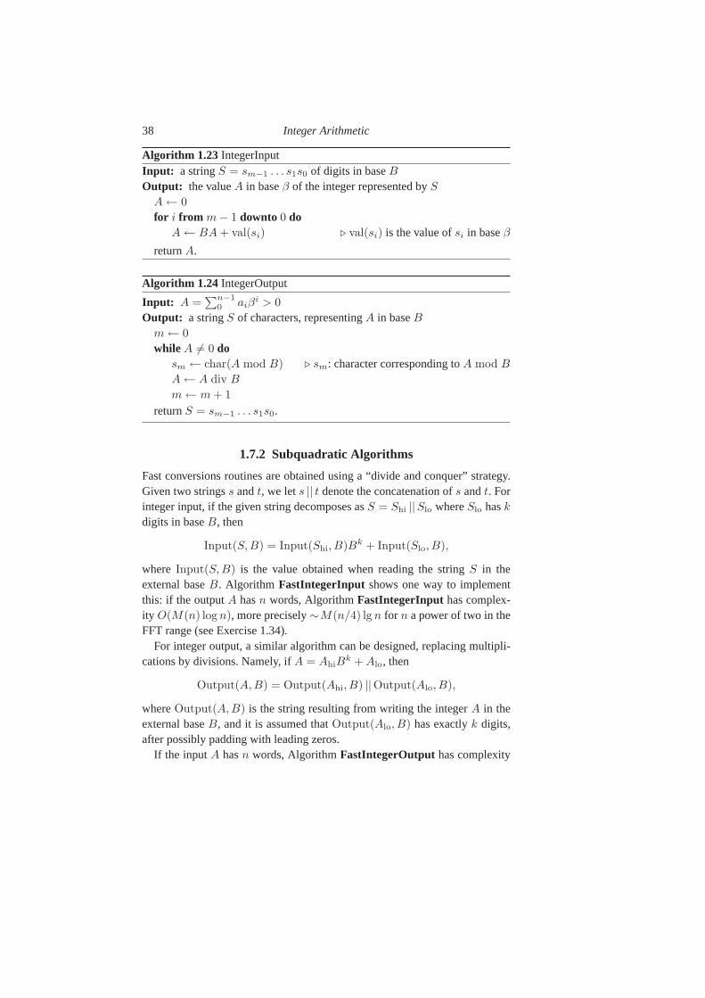
38 Integer Arithmetic
Algorithm 1.23 IntegerInputInput: a stringS = sm−1 . . . s1s0 of digits in baseBOutput: the valueA in baseβ of the integer represented byS
A ← 0
for i from m − 1 downto 0 doA ← BA + val(si) ⊲ val(si) is the value ofsi in baseβ
returnA.
Algorithm 1.24 IntegerOutput
Input: A =∑n−1
0 aiβi > 0
Output: a stringS of characters, representingA in baseBm ← 0
while A 6= 0 dosm ← char(A mod B) ⊲ sm: character corresponding toA mod B
A ← A div B
m ← m + 1
returnS = sm−1 . . . s1s0.
1.7.2 Subquadratic Algorithms
Fast conversions routines are obtained using a “divide and conquer” strategy.Given two stringss andt, we lets || t denote the concatenation ofs andt. Forinteger input, if the given string decomposes asS = Shi ||Slo whereSlo haskdigits in baseB, then
Input(S,B) = Input(Shi, B)Bk + Input(Slo, B),
where Input(S,B) is the value obtained when reading the stringS in theexternal baseB. Algorithm FastIntegerInput shows one way to implementthis: if the outputA hasn words, AlgorithmFastIntegerInput has complex-ity O(M(n) log n), more precisely∼M(n/4) lg n for n a power of two in theFFT range (see Exercise 1.34).
For integer output, a similar algorithm can be designed, replacing multipli-cations by divisions. Namely, ifA = AhiB
k + Alo, then
Output(A,B) = Output(Ahi, B) ||Output(Alo, B),
whereOutput(A,B) is the string resulting from writing the integerA in theexternal baseB, and it is assumed thatOutput(Alo, B) has exactlyk digits,after possibly padding with leading zeros.
If the inputA hasn words, AlgorithmFastIntegerOutput has complexity
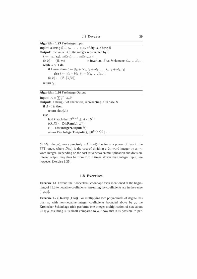
1.8 Exercises 39
Algorithm 1.25 FastIntegerInputInput: a stringS = sm−1 . . . s1s0 of digits in baseBOutput: the valueA of the integer represented byS
ℓ ← [val(s0), val(s1), . . . , val(sm−1)]
(b, k) ← (B,m) ⊲ Invariant:ℓ hask elementsℓ0, . . . , ℓk−1
while k > 1 doif k eventhen ℓ ← [ℓ0 + bℓ1, ℓ2 + bℓ3, . . . , ℓk−2 + bℓk−1]
elseℓ ← [ℓ0 + bℓ1, ℓ2 + bℓ3, . . . , ℓk−1]
(b, k) ← (b2, ⌈k/2⌉)returnℓ0.
Algorithm 1.26 FastIntegerOutput
Input: A =∑n−1
0 aiβi
Output: a stringS of characters, representingA in baseBif A < B then
returnchar(A)
elsefind k such thatB2k−2 ≤ A < B2k
(Q,R) ← DivRem(A,Bk)
r ← FastIntegerOutput(R)
returnFastIntegerOutput(Q) || 0k−len(r) || r.
O(M(n) log n), more precisely∼D(n/4) lg n for n a power of two in theFFT range, whereD(n) is the cost of dividing a2n-word integer by ann-word integer. Depending on the cost ratio between multiplication and division,integer output may thus be from2 to 5 times slower than integer input; seehowever Exercise 1.35.
1.8 Exercises
Exercise 1.1Extend the Kronecker-Schonhage trick mentioned at the begin-ning of§1.3 to negative coefficients, assuming the coefficients are in the range[−ρ, ρ].
Exercise 1.2 (Harvey[114]) For multiplying two polynomials of degree lessthan n, with non-negative integer coefficients bounded above byρ, theKronecker-Schonhage trick performs one integer multiplication of size about2n lg ρ, assumingn is small compared toρ. Show that it is possible to per-
40 Integer Arithmetic
form two integer multiplications of sizen lg ρ instead, and even four integermultiplications of size(n/2) lg ρ.
Exercise 1.3Assume your processor provides an instructionfmaa (a, b, c, d)
returningh, ℓ such thatab + c + d = hβ + ℓ where0 ≤ a, b, c, d, ℓ, h < β.Rewrite AlgorithmBasecaseMultiplyusingfmaa .
Exercise 1.4 (Harvey, Khachatrianet al.[139]) For A =∑n−1
i=0 aiβi and
B =∑n−1
j=0 biβi, prove the formula:
AB =
n−1∑
i=1
i−1∑
j=0
(ai + aj)(bi + bj)βi+j + 2
n−1∑
i=0
aibiβ2i −
n−1∑
i=0
βin−1∑
j=0
ajbjβj .
Deduce a new algorithm for schoolbook multiplication.
Exercise 1.5 (Hanrot) Prove that the numberK(n) of word products (as de-fined in the proof of Thm. 1.3.2) in Karatsuba’s algorithm is non-decreasing,providedn0 = 2. Plot the graph ofK(n)/nlg 3 with a logarithmic scale forn,for 27 ≤ n ≤ 210, and find experimentally where the maximum appears.
Exercise 1.6 (Ryde)Assume the basecase multiply costsM(n) = an2 + bn,and that Karatsuba’s algorithm costsK(n) = 3K(n/2)+cn. Show that divid-ing a by two increases the Karatsuba thresholdn0 by a factor of two, and onthe contrary decreasingb andc decreasesn0.
Exercise 1.7 (Maeder[158], Thome [216]) Show that an auxiliary memoryof 2n + o(n) words is enough to implement Karatsuba’s algorithm in-place,for ann-word×n-word product. In the polynomial case, prove that an auxiliaryspace ofn coefficients is enough, in addition to then + n coefficients of theinput polynomials, and the2n− 1 coefficients of the product. [You can use the2n result words, but must not destroy then + n input words.]
Exercise 1.8 (Roche[191]) If Exercise 1.7 was too easy for you, design aKaratsuba-like algorithm using onlyO(log n) extra space (you are allowed toread and write in the2n output words, but then+n input words are read-only).
Exercise 1.9 (Quercia, McLaughlin)Modify Algorithm KaratsubaMultiplyto use only∼7n/2 additions/subtractions. [Hint: decompose each ofC0, C1
andC2 into two parts.]
Exercise 1.10Design an in-place version ofKaratsubaMultiply (see Exer-cise 1.7) that accumulates the result inc0, . . . , cn−1, and returns a carry bit.
1.8 Exercises 41
Exercise 1.11 (Vuillemin) Design an algorithm to multiplya2x2+a1x+a0 by
b1x+ b0 using4 multiplications. Can you extend it to a6× 6 product using16
multiplications?
Exercise 1.12 (Weimerskirch, Paar)Extend the Karatsuba trick to computean n × n product inn(n + 1)/2 multiplications. For whichn does this winover the classical Karatsuba algorithm?
Exercise 1.13 (Hanrot) In Algorithm OddEvenKaratsuba, if both m andn
are odd, one combines the larger partsA0 andB0 together, and the smallerpartsA1 andB1 together. Find a way to get instead:
K(m,n) = K(⌈m/2⌉, ⌊n/2⌋) + K(⌊m/2⌋, ⌈n/2⌉) + K(⌈m/2⌉, ⌈n/2⌉).
Exercise 1.14Prove that if5 integer evaluation points are used for Toom-Cook 3-way (§1.3.3), the division by (a multiple of)3 can not be avoided.Does this remain true if only4 integer points are used together with∞?
Exercise 1.15 (Quercia, Harvey)In Toom-Cook3-way (§1.3.3), take as eval-uation point2w instead of2, wherew is the number of bits per word (usuallyw = 32 or 64). Which division is then needed? Similarly for the evaluationpoint2w/2.
Exercise 1.16For an integerk ≥ 2 and multiplication of two numbers of sizekn andn, show that the trivial strategy which performsk multiplications, eachn × n, is not the best possible in the FFT range.
Exercise 1.17 (Karatsuba, Zuras[236]) Assuming the multiplication has su-perlinear cost, show that the speedup of squaring with respect to multiplicationcan not significantly exceed2.
Exercise 1.18 (Thome, Quercia) Consider two setsA = a, b, c, . . . andU = u, v, w, . . ., and a setX = x, y, z, . . . of sums of products of el-ements ofA andU (assumed to be in some fieldF ). We can ask “what isthe least number of multiplies required to compute all elements of X?”. Ingeneral, this is a difficult problem, related to the problem of computing tensorrank, which is NP-complete (see for example Hastad [119] and the book byBurgisseret al. [59]). Special cases include integer/polynomial multiplication,the middle product, and matrix multiplication (for matrices of fixed size). As aspecific example, can we computex = au+ cw, y = av + bw, z = bu+ cv infewer than6 multiplies? Similarly forx = au−cw, y = av−bw, z = bu−cv.
Exercise 1.19In Algorithm BasecaseDivRem(§1.4.1), prove thatq∗j ≤ β+1.Can this bound be reached? In the caseq∗j ≥ β, prove that the while-loop at

42 Integer Arithmetic
steps 6-8 is executed at most once. Prove that the same holds for Svoboda’salgorithm, i.e., thatA ≥ 0 after step 8 of AlgorithmSvobodaDivision(§1.4.2).
Exercise 1.20 (Granlund, Moller) In Algorithm BasecaseDivRem, estimatethe probability thatA < 0 is true at step 6, assuming the remainderrj from thedivision ofan+jβ + an+j−1 by bn−1 is uniformly distributed in[0, bn−1 − 1],A mod βn+j−1 is uniformly distributed in[0, βn+j−1 − 1], andB mod βn−1
is uniformly distributed in[0, βn−1−1]. Then replace the computation ofq∗j bya division of the three most significant words ofA by the two most significantwords ofB. Prove the algorithm is still correct. What is the maximal numberof corrections, and the probability thatA < 0?
Exercise 1.21 (Montgomery[172]) Let 0 < b < β, and0 ≤ a4, . . . , a0 < β.Prove thata4(β
4 mod b) + · · ·+ a1(β mod b) + a0 < β2, providedb < β/3.Use this fact to design an efficient algorithm dividingA = an−1β
n−1+· · ·+a0
by b. Does the algorithm extend to division by the least significant digits?
Exercise 1.22In Algorithm RecursiveDivRem, find inputs that require1, 2, 3or 4 corrections in step 8. [Hint: considerβ = 2.] Prove that whenn = m andA < βm(B + 1), at most two corrections occur.
Exercise 1.23Find the complexity of AlgorithmRecursiveDivRem in theFFT range.
Exercise 1.24Consider the division ofA of kn words byB of n words, withintegerk ≥ 3, and the alternate strategy that consists of extending the divisorwith zeros so that it has half the size of the dividend. Show that this is al-ways slower than AlgorithmUnbalancedDivision[assuming that division hassuperlinear cost].
Exercise 1.25An important special base of division is when the divisor is ofthe formbk. For example, this is useful for an integer output routine (§1.7).Can one design a fast algorithm for this case?
Exercise 1.26 (Sedoglavic)Does the Kronecker-Schonhage trick to reducepolynomial multiplication to integer multiplication (§1.3) also work — in anefficient way — for division? Assume that you want to divide a degree-2n
polynomialA(x) by a monic degree-n polynomialB(x), both polynomialshaving integer coefficients bounded byρ.
Exercise 1.27Design an algorithm that performs an exact division of a4n-bitinteger by a2n-bit integer, with a quotient of2n bits, using the idea mentionedin the last paragraph of§1.4.5. Prove that your algorithm is correct.
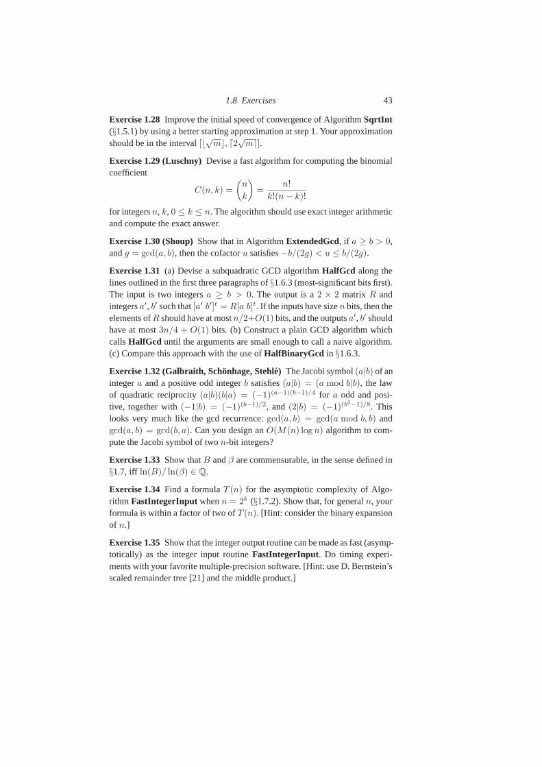
1.8 Exercises 43
Exercise 1.28Improve the initial speed of convergence of AlgorithmSqrtInt(§1.5.1) by using a better starting approximation at step 1. Your approximationshould be in the interval[⌊√m⌋, ⌈2√m⌉].
Exercise 1.29 (Luschny)Devise a fast algorithm for computing the binomialcoefficient
C(n, k) =
(n
k
)=
n!
k!(n − k)!
for integersn, k, 0 ≤ k ≤ n. The algorithm should use exact integer arithmeticand compute the exact answer.
Exercise 1.30 (Shoup)Show that in AlgorithmExtendedGcd, if a ≥ b > 0,andg = gcd(a, b), then the cofactoru satisfies−b/(2g) < u ≤ b/(2g).
Exercise 1.31(a) Devise a subquadratic GCD algorithmHalfGcd along thelines outlined in the first three paragraphs of§1.6.3 (most-significant bits first).The input is two integersa ≥ b > 0. The output is a2 × 2 matrix R andintegersa′, b′ such that[a′ b′]t = R[a b]t. If the inputs have sizen bits, then theelements ofR should have at mostn/2+O(1) bits, and the outputsa′, b′ shouldhave at most3n/4 + O(1) bits. (b) Construct a plain GCD algorithm whichcallsHalfGcd until the arguments are small enough to call a naive algorithm.(c) Compare this approach with the use ofHalfBinaryGcd in §1.6.3.
Exercise 1.32 (Galbraith, Schonhage, Stehle) The Jacobi symbol(a|b) of anintegera and a positive odd integerb satisfies(a|b) = (a mod b|b), the lawof quadratic reciprocity(a|b)(b|a) = (−1)(a−1)(b−1)/4 for a odd and posi-tive, together with(−1|b) = (−1)(b−1)/2, and(2|b) = (−1)(b
2−1)/8. Thislooks very much like the gcd recurrence:gcd(a, b) = gcd(a mod b, b) andgcd(a, b) = gcd(b, a). Can you design anO(M(n) log n) algorithm to com-pute the Jacobi symbol of twon-bit integers?
Exercise 1.33Show thatB andβ are commensurable, in the sense defined in§1.7, iff ln(B)/ ln(β) ∈ Q.
Exercise 1.34Find a formulaT (n) for the asymptotic complexity of Algo-rithm FastIntegerInput whenn = 2k (§1.7.2). Show that, for generaln, yourformula is within a factor of two ofT (n). [Hint: consider the binary expansionof n.]
Exercise 1.35Show that the integer output routine can be made as fast (asymp-totically) as the integer input routineFastIntegerInput. Do timing experi-ments with your favorite multiple-precision software. [Hint: use D. Bernstein’sscaled remainder tree [21] and the middle product.]
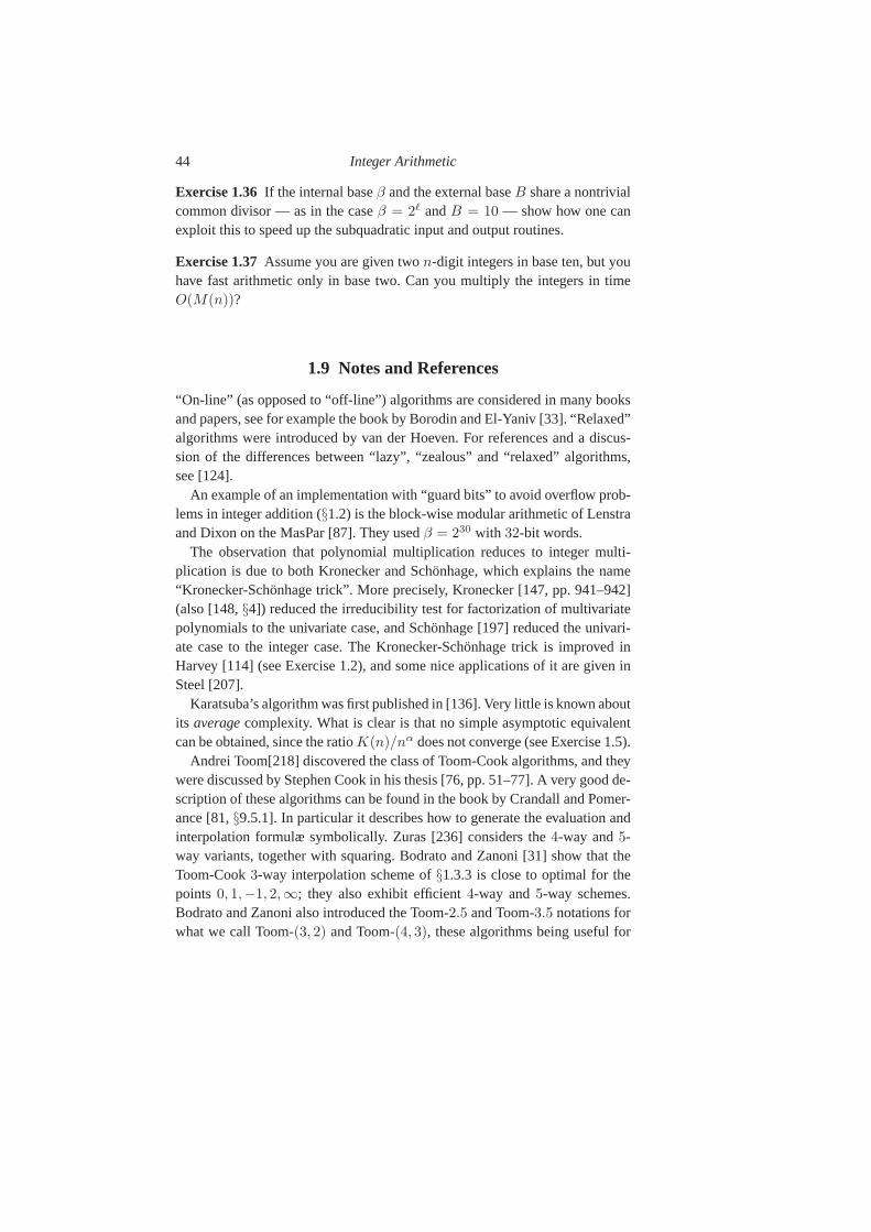
44 Integer Arithmetic
Exercise 1.36If the internal baseβ and the external baseB share a nontrivialcommon divisor — as in the caseβ = 2ℓ andB = 10 — show how one canexploit this to speed up the subquadratic input and output routines.
Exercise 1.37Assume you are given twon-digit integers in base ten, but youhave fast arithmetic only in base two. Can you multiply the integers in timeO(M(n))?
1.9 Notes and References
“On-line” (as opposed to “off-line”) algorithms are considered in many booksand papers, see for example the book by Borodin and El-Yaniv [33]. “Relaxed”algorithms were introduced by van der Hoeven. For references and a discus-sion of the differences between “lazy”, “zealous” and “relaxed” algorithms,see [124].
An example of an implementation with “guard bits” to avoid overflow prob-lems in integer addition (§1.2) is the block-wise modular arithmetic of Lenstraand Dixon on the MasPar [87]. They usedβ = 230 with 32-bit words.
The observation that polynomial multiplication reduces tointeger multi-plication is due to both Kronecker and Schonhage, which explains the name“Kronecker-Schonhage trick”. More precisely, Kronecker [147, pp. 941–942](also [148,§4]) reduced the irreducibility test for factorization of multivariatepolynomials to the univariate case, and Schonhage [197] reduced the univari-ate case to the integer case. The Kronecker-Schonhage trick is improved inHarvey [114] (see Exercise 1.2), and some nice applicationsof it are given inSteel [207].
Karatsuba’s algorithm was first published in [136]. Very little is known aboutits averagecomplexity. What is clear is that no simple asymptotic equivalentcan be obtained, since the ratioK(n)/nα does not converge (see Exercise 1.5).
Andrei Toom[218] discovered the class of Toom-Cook algorithms, and theywere discussed by Stephen Cook in his thesis [76, pp. 51–77].A very good de-scription of these algorithms can be found in the book by Crandall and Pomer-ance [81,§9.5.1]. In particular it describes how to generate the evaluation andinterpolation formulæ symbolically. Zuras [236] considers the4-way and5-way variants, together with squaring. Bodrato and Zanoni [31] show that theToom-Cook3-way interpolation scheme of§1.3.3 is close to optimal for thepoints 0, 1,−1, 2,∞; they also exhibit efficient4-way and5-way schemes.Bodrato and Zanoni also introduced the Toom-2.5 and Toom-3.5 notations forwhat we call Toom-(3, 2) and Toom-(4, 3), these algorithms being useful for
1.9 Notes and References 45
unbalanced multiplication using a different number of pieces. They noticedthat Toom-(4, 2) only differs from Toom3-way in the evaluation phase, thusmost of the implementation can be shared.
The Schonhage-Strassen algorithm first appeared in [200], and is describedin §2.3.3. Algorithms using floating-point complex numbers arediscussed inKnuth’s classic [143,§4.3.3.C]. See also§3.3.1.
The odd-even scheme is described in Hanrot and Zimmermann [112], andwas independently discovered by Andreas Enge. The asymmetric squaring for-mula given in§1.3.6 was invented by Chung and Hasan (see their paper [66]for other asymmetric formulæ). Exercise 1.4 was suggested by David Harvey,who independently discovered the algorithm of Khachatrianet al. [139].
See Lefevre [153] for a comparison of different algorithms for the problemof multiplication by an integer constant.
Svoboda’s algorithm was introduced in [212]. The exact division algorithmstarting from least significant bits is due to Jebelean [130]. Jebelean andKrandick invented the “bidirectional” algorithm [145]. The Karp-Marksteintrick to speed up Newton’s iteration (or Hensel lifting overp-adic numbers)is described in [138]. The “recursive division” of§1.4.3 is from Burnikel andZiegler [60], although earlier but not-so-detailed ideas can be found in Jebe-lean [132], and even earlier in Moenck and Borodin [167]. Thedefinition ofHensel’s division used here is due to Shand and Vuillemin [202], who alsopoint out the duality with Euclidean division.
Algorithm SqrtRem (§1.5.1) was first described in Zimmermann [235], andproved correct in Bertotet al. [29]. Algorithm SqrtInt is described in [73]; itsgeneralization tok-th roots (AlgorithmRootInt ) is due to Keith Briggs. Thedetection of exact powers is discussed in Bernstein, Lenstra and Pila [23] andearlier in Bernstein [17] and Cohen [73]. It is necessary, for example, in theAKS primality test [2].
The classical (quadratic) Euclidean algorithm has been considered by manyauthors — a good reference is Knuth [143]. The Gauss-Kuz’mintheorem2
gives the distribution of quotients in the regular continued fraction of almostall real numbers, and hence is a good guide to the distribution of quotients inthe Euclidean algorithm for large, random inputs. Lehmer’soriginal algorithmis described in [155]. The binary gcd is almost as old as the classical Euclideanalgorithm — Knuth [143] has traced it back to a first-century AD Chinese textChiu Chang Suan Shu(see also Mikami [166]). It was rediscovered severaltimes in the 20th century, and it is usually attributed to Stein [210]. The bi-nary gcd has been analysed by Brent [44, 50], Knuth [143], Maze [160] and
2 According to the Gauss-Kuz’min theorem [140], the probability of a quotientq ∈ N∗ islg(1 + 1/q) − lg(1 + 1/(q + 1)).
46 Integer Arithmetic
Vallee [222]. A parallel (systolic) version that runs inO(n) time usingO(n)
processors was given by Brent and Kung [53].The double-digit gcd is due to Jebelean [131]. Thek-ary gcd reduction is
due to Sorenson [206], and was improved and implemented in GNU MP byWeber. Weber also invented AlgorithmReducedRatMod [227], inspired byprevious work of Wang.
The first subquadratic gcd algorithm was published by Knuth [142], buthis complexity analysis was suboptimal — he gaveO(n log5 n log log n). Thecorrect complexityO(n log2 n log log n) was given by Schonhage [196]; forthis reason the algorithm is sometimes called the Knuth-Schonhage algorithm.A description for the polynomial case can be found in Aho, Hopcroft andUllman [3], and a detailed (but incorrect) description for the integer case inYap [233]. The subquadratic binary gcd given in§1.6.3 is due to Stehle andZimmermann [209]. Moller [169] compares various subquadratic algorithms,and gives a nice algorithm without “repair steps”.
Several authors mention anO(n log2 n log log n) algorithm for the compu-tation of the Jacobi symbol [89, 201]. The earliest reference that we know isa paper by Bach [8], which gives the basic idea (due to Gauss [101, p. 509]).Details are given in the book by Bach and Shallit [9, Solutionof Exercise5.52], where the algorithm is said to be “folklore”, with theideas going backto Bachmann [10] and Gauss. The existence of such an algorithm is mentionedin Schonhage’s book [199,§7.2.3], but without details. See also Exercise 1.32.
2
Modular Arithmetic and the FFT
In this chapter our main topic is modular arithmetic, i.e., howto compute efficiently modulo a given integerN . In most appli-cations, the modulusN is fixed, and special-purpose algorithmsbenefit from some precomputations, depending only onN , tospeed up arithmetic moduloN .There is an overlap between Chapter 1 and this chapter. For ex-ample, integer division and modular multiplication are closely re-lated. In Chapter 1 we present algorithms where no (or only a few)precomputations with respect to the modulusN are performed. Inthis chapter we consider algorithms which benefit from such pre-computations.Unless explicitly stated, we consider that the modulusN occupiesn words in the word-baseβ, i.e.,βn−1 ≤ N < βn.
2.1 Representation
We consider in this section the different possible representations of residuesmoduloN . As in Chapter 1, we consider mainly dense representations.
2.1.1 Classical Representation
The classical representation stores a residue (class)a as an integer0 ≤ a < N .Residues are thus always fully reduced, i.e., incanonicalform.
Another non-redundant form consists in choosing a symmetric representa-tion, say−N/2 ≤ a < N/2. This form might save some reductions in addi-tions or subtractions (see§2.2). Negative numbers might be stored either witha separate sign (sign-magnitude representation) or with a two’s-complementrepresentation.
48 Modular Arithmetic and the FFT
SinceN takesn words in baseβ, an alternativeredundantrepresentationchooses0 ≤ a < βn to represent a residue class. If the underlying arithmeticis word-based, this will yield no slowdown compared to the canonical form. Anadvantage of this representation is that, when adding two residues, it suffices tocompare their sum toβn in order to decide whether the sum has to be reduced,and the result of this comparison is simply given by the carrybit of the addition(see AlgorithmIntegerAddition in §1.2), instead of by comparing the sumwith N . However, in the case that the sum has to be reduced, one or morefurther comparisons are needed.
2.1.2 Montgomery’s Form
Montgomery’s form is another representation widely used when several mod-ular operations have to be performed modulo the same integerN (additions,subtractions, modular multiplications). It implies a small overhead to convert— if needed — from the classical representation to Montgomery’s and vice-versa, but this overhead is often more than compensated by the speedup ob-tained in the modular multiplication.
The main idea is to represent a residuea by a′ = aR mod N , whereR = βn, andN takesn words in baseβ. Thus Montgomery is not concernedwith the physicalrepresentation of a residue class, but with themeaningas-sociated to a given physical representation. (As a consequence, the differentchoices mentioned above for the physical representation are all possible.) Ad-dition and subtraction are unchanged, but (modular) multiplication translatesto a different, much simpler, algorithm (§2.4.2).
In most applications using Montgomery’s form, all inputs are first convertedto Montgomery’s form, usinga′ = aR mod N , then all computations are per-formed in Montgomery’s form, and finally all outputs are converted back — ifneeded — to the classical form, usinga = a′/R mod N . We need to assumethat (R,N) = 1, or equivalently that(β,N) = 1, to ensure the existence of1/R mod N . This is not usually a problem becauseβ is a power of two andN can be assumed to be odd.
2.1.3 Residue Number Systems
In a Residue Number System, a residuea is represented by a list of residuesai moduloNi, where the moduliNi are coprime and their product isN . Theintegersai can be efficiently computed froma using a remainder tree, and theunique integer0 ≤ a < N = N1N2 · · · is computed from theai by an Ex-plicit Chinese Remainder Theorem (§2.7). The residue number system is inter-
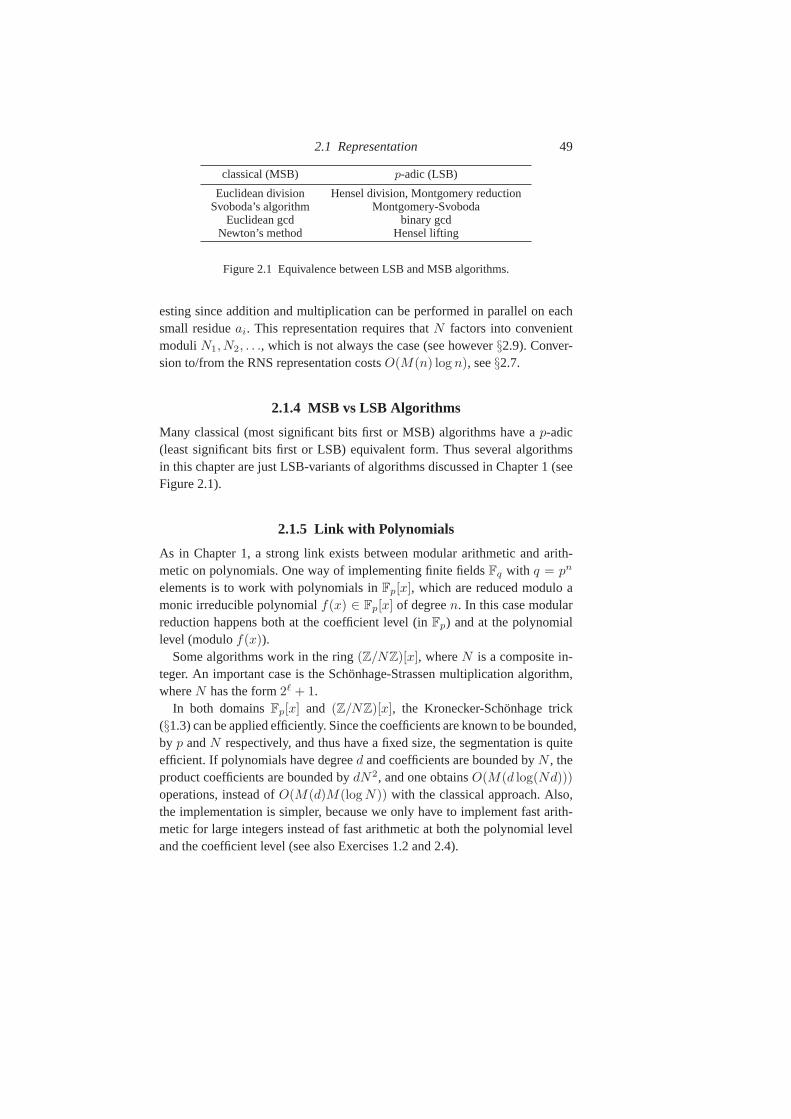
2.1 Representation 49
classical (MSB) p-adic (LSB)
Euclidean division Hensel division, Montgomery reductionSvoboda’s algorithm Montgomery-Svoboda
Euclidean gcd binary gcdNewton’s method Hensel lifting
Figure 2.1 Equivalence between LSB and MSB algorithms.
esting since addition and multiplication can be performed in parallel on eachsmall residueai. This representation requires thatN factors into convenientmoduli N1, N2, . . ., which is not always the case (see however§2.9). Conver-sion to/from the RNS representation costsO(M(n) log n), see§2.7.
2.1.4 MSB vs LSB Algorithms
Many classical (most significant bits first or MSB) algorithms have ap-adic(least significant bits first or LSB) equivalent form. Thus several algorithmsin this chapter are just LSB-variants of algorithms discussed in Chapter 1 (seeFigure 2.1).
2.1.5 Link with Polynomials
As in Chapter 1, a strong link exists between modular arithmetic and arith-metic on polynomials. One way of implementing finite fieldsFq with q = pn
elements is to work with polynomials inFp[x], which are reduced modulo amonic irreducible polynomialf(x) ∈ Fp[x] of degreen. In this case modularreduction happens both at the coefficient level (inFp) and at the polynomiallevel (modulof(x)).
Some algorithms work in the ring(Z/NZ)[x], whereN is a composite in-teger. An important case is the Schonhage-Strassen multiplication algorithm,whereN has the form2ℓ + 1.
In both domainsFp[x] and (Z/NZ)[x], the Kronecker-Schonhage trick(§1.3) can be applied efficiently. Since the coefficients are known to be bounded,by p andN respectively, and thus have a fixed size, the segmentation isquiteefficient. If polynomials have degreed and coefficients are bounded byN , theproduct coefficients are bounded bydN2, and one obtainsO(M(d log(Nd)))
operations, instead ofO(M(d)M(log N)) with the classical approach. Also,the implementation is simpler, because we only have to implement fast arith-metic for large integers instead of fast arithmetic at both the polynomial leveland the coefficient level (see also Exercises 1.2 and 2.4).
50 Modular Arithmetic and the FFT
2.2 Modular Addition and Subtraction
The addition of two residues in classical representation can be done as in Al-gorithmModularAdd .
Algorithm 2.1 ModularAddInput: residuesa, b with 0 ≤ a, b < N
Output: c = a + b mod N
c ← a + b
if c ≥ N thenc ← c − N .
Assuming thata andb are uniformly distributed inZ ∩ [0, N − 1], the sub-tractionc ← c − N is performed with probability(1 − 1/N)/2. If we useinstead a symmetric representation in[−N/2, N/2), the probability that weneed to add or subtractN drops to1/4 + O(1/N2) at the cost of an additionaltest. This extra test might be expensive for smallN — say one or two words— but should be relatively cheap ifN is large enough, say at least ten words.
2.3 The Fourier Transform
In this section we introduce the discrete Fourier transform(DFT). An impor-tant application of the DFT is in computing convolutions viatheConvolutionTheorem. In general, the convolution of two vectors can be computed usingthree DFTs (for details see§2.9). Here we show how to compute the DFT effi-ciently (via theFast Fourier Transformor FFT), and show how it can be usedto multiply two n-bit integers in timeO(n log n log log n) (the Schonhage-Strassen algorithm, see§2.3.3).
2.3.1 Theoretical Setting
Let R be a ring,K ≥ 2 an integer, andω a K-th principal root of unity inR, i.e., such thatωK = 1 and
∑K−1j=0 ωij = 0 for 1 ≤ i < K. TheFourier
transform(or forward (Fourier) transform) of a vectora = [a0, a1, . . . , aK−1]
of K elements fromR is the vectora = [a0, a1, . . . , aK−1] such that
ai =
K−1∑
j=0
ωijaj . (2.1)
If we transform the vectora twice, we get back to the initial vector, apart
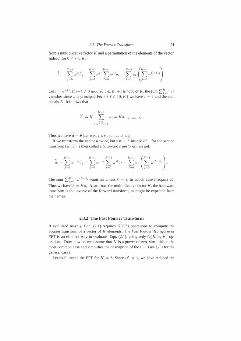
2.3 The Fourier Transform 51
from a multiplicative factorK and a permutation of the elements of the vector.Indeed, for0 ≤ i < K,
ai =
K−1∑
j=0
ωij aj =
K−1∑
j=0
ωijK−1∑
ℓ=0
ωjℓaℓ =
K−1∑
ℓ=0
aℓ
K−1∑
j=0
ω(i+ℓ)j
.
Let τ = ωi+ℓ. If i+ℓ 6= 0 mod K, i.e., if i+ℓ is not0 orK, the sum∑K−1
j=0 τ j
vanishes sinceω is principal. Fori + ℓ ∈ 0,K we haveτ = 1 and the sumequalsK. It follows that
ai = K
K−1∑
ℓ=0
i+ℓ∈0,K
aℓ = Ka(−i) mod K .
Thus we havea = K[a0, aK−1, aK−2, . . . , a2, a1].If we transform the vectora twice, but useω−1 instead ofω for the second
transform (which is then called abackward transform), we get:
˜ai =
K−1∑
j=0
ω−ij aj =
K−1∑
j=0
ω−ijK−1∑
ℓ=0
ωjℓaℓ =
K−1∑
ℓ=0
aℓ
K−1∑
j=0
ω(ℓ−i)j
.
The sum∑K−1
j=0 ω(ℓ−i)j vanishes unlessℓ = i, in which case it equalsK.
Thus we haveai = Kai. Apart from the multiplicative factorK, the backwardtransform is the inverse of the forward transform, as might be expected fromthe names.
2.3.2 The Fast Fourier Transform
If evaluated naively, Eqn. (2.1) requiresΩ(K2) operations to compute theFourier transform of a vector ofK elements. TheFast Fourier TransformorFFT is an efficient way to evaluate Eqn. (2.1), using onlyO(K log K) op-erations. From now on we assume thatK is a power of two, since this is themost common case and simplifies the description of the FFT (see §2.9 for thegeneral case).
Let us illustrate the FFT forK = 8. Sinceω8 = 1, we have reduced the
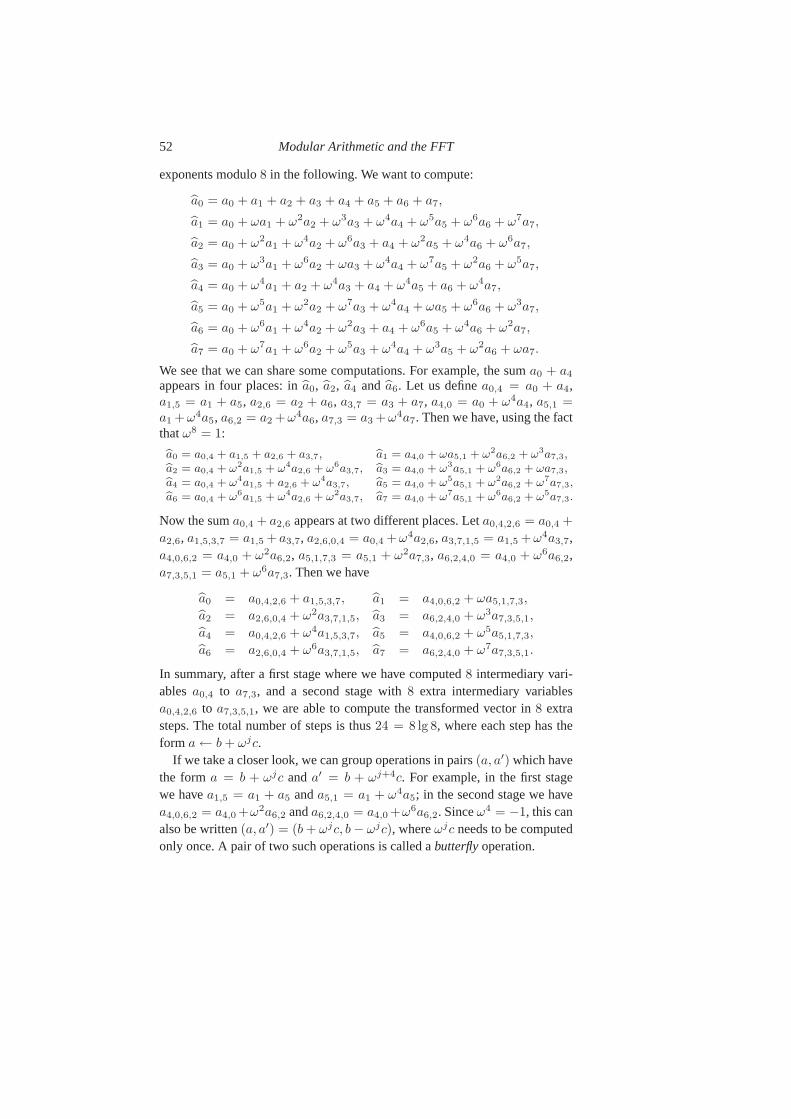
52 Modular Arithmetic and the FFT
exponents modulo8 in the following. We want to compute:
a0 = a0 + a1 + a2 + a3 + a4 + a5 + a6 + a7,
a1 = a0 + ωa1 + ω2a2 + ω3a3 + ω4a4 + ω5a5 + ω6a6 + ω7a7,
a2 = a0 + ω2a1 + ω4a2 + ω6a3 + a4 + ω2a5 + ω4a6 + ω6a7,
a3 = a0 + ω3a1 + ω6a2 + ωa3 + ω4a4 + ω7a5 + ω2a6 + ω5a7,
a4 = a0 + ω4a1 + a2 + ω4a3 + a4 + ω4a5 + a6 + ω4a7,
a5 = a0 + ω5a1 + ω2a2 + ω7a3 + ω4a4 + ωa5 + ω6a6 + ω3a7,
a6 = a0 + ω6a1 + ω4a2 + ω2a3 + a4 + ω6a5 + ω4a6 + ω2a7,
a7 = a0 + ω7a1 + ω6a2 + ω5a3 + ω4a4 + ω3a5 + ω2a6 + ωa7.
We see that we can share some computations. For example, the sum a0 + a4
appears in four places: ina0, a2, a4 and a6. Let us definea0,4 = a0 + a4,a1,5 = a1 + a5, a2,6 = a2 + a6, a3,7 = a3 + a7, a4,0 = a0 + ω4a4, a5,1 =a1 +ω4a5, a6,2 = a2 +ω4a6, a7,3 = a3 +ω4a7. Then we have, using the factthatω8 = 1:
ba0 = a0,4 + a1,5 + a2,6 + a3,7, ba1 = a4,0 + ωa5,1 + ω2a6,2 + ω3a7,3,ba2 = a0,4 + ω2a1,5 + ω4a2,6 + ω6a3,7, ba3 = a4,0 + ω3a5,1 + ω6a6,2 + ωa7,3,ba4 = a0,4 + ω4a1,5 + a2,6 + ω4a3,7, ba5 = a4,0 + ω5a5,1 + ω2a6,2 + ω7a7,3,ba6 = a0,4 + ω6a1,5 + ω4a2,6 + ω2a3,7, ba7 = a4,0 + ω7a5,1 + ω6a6,2 + ω5a7,3.
Now the suma0,4 + a2,6 appears at two different places. Leta0,4,2,6 = a0,4 +
a2,6, a1,5,3,7 = a1,5 + a3,7, a2,6,0,4 = a0,4 +ω4a2,6, a3,7,1,5 = a1,5 +ω4a3,7,a4,0,6,2 = a4,0 + ω2a6,2, a5,1,7,3 = a5,1 + ω2a7,3, a6,2,4,0 = a4,0 + ω6a6,2,a7,3,5,1 = a5,1 + ω6a7,3. Then we have
a0 = a0,4,2,6 + a1,5,3,7, a1 = a4,0,6,2 + ωa5,1,7,3,
a2 = a2,6,0,4 + ω2a3,7,1,5, a3 = a6,2,4,0 + ω3a7,3,5,1,
a4 = a0,4,2,6 + ω4a1,5,3,7, a5 = a4,0,6,2 + ω5a5,1,7,3,
a6 = a2,6,0,4 + ω6a3,7,1,5, a7 = a6,2,4,0 + ω7a7,3,5,1.
In summary, after a first stage where we have computed8 intermediary vari-ablesa0,4 to a7,3, and a second stage with8 extra intermediary variablesa0,4,2,6 to a7,3,5,1, we are able to compute the transformed vector in8 extrasteps. The total number of steps is thus24 = 8 lg 8, where each step has theform a ← b + ωjc.
If we take a closer look, we can group operations in pairs(a, a′) which havethe forma = b + ωjc anda′ = b + ωj+4c. For example, in the first stagewe havea1,5 = a1 + a5 anda5,1 = a1 + ω4a5; in the second stage we havea4,0,6,2 = a4,0 +ω2a6,2 anda6,2,4,0 = a4,0 +ω6a6,2. Sinceω4 = −1, this canalso be written(a, a′) = (b + ωjc, b − ωjc), whereωjc needs to be computedonly once. A pair of two such operations is called abutterflyoperation.
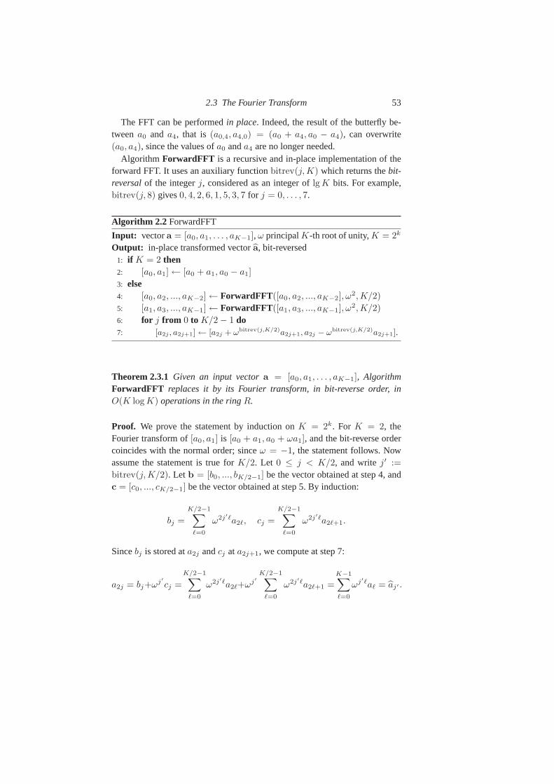
2.3 The Fourier Transform 53
The FFT can be performedin place. Indeed, the result of the butterfly be-tweena0 and a4, that is (a0,4, a4,0) = (a0 + a4, a0 − a4), can overwrite(a0, a4), since the values ofa0 anda4 are no longer needed.
Algorithm ForwardFFT is a recursive and in-place implementation of theforward FFT. It uses an auxiliary functionbitrev(j,K) which returns thebit-reversalof the integerj, considered as an integer oflg K bits. For example,bitrev(j, 8) gives0, 4, 2, 6, 1, 5, 3, 7 for j = 0, . . . , 7.
Algorithm 2.2 ForwardFFT
Input: vectora = [a0, a1, . . . , aK−1], ω principalK-th root of unity,K = 2k
Output: in-place transformed vectora, bit-reversed1: if K = 2 then2: [a0, a1] ← [a0 + a1, a0 − a1]
3: else4: [a0, a2, ..., aK−2] ← ForwardFFT ([a0, a2, ..., aK−2], ω
2,K/2)
5: [a1, a3, ..., aK−1] ← ForwardFFT ([a1, a3, ..., aK−1], ω2,K/2)
6: for j from 0 to K/2 − 1 do7: [a2j , a2j+1] ← [a2j + ωbitrev(j,K/2)a2j+1, a2j − ωbitrev(j,K/2)a2j+1].
Theorem 2.3.1 Given an input vectora = [a0, a1, . . . , aK−1], AlgorithmForwardFFT replaces it by its Fourier transform, in bit-reverse order,inO(K log K) operations in the ringR.
Proof. We prove the statement by induction onK = 2k. For K = 2, theFourier transform of[a0, a1] is [a0 + a1, a0 + ωa1], and the bit-reverse ordercoincides with the normal order; sinceω = −1, the statement follows. Nowassume the statement is true forK/2. Let 0 ≤ j < K/2, and writej′ :=
bitrev(j,K/2). Let b = [b0, ..., bK/2−1] be the vector obtained at step 4, andc = [c0, ..., cK/2−1] be the vector obtained at step 5. By induction:
bj =
K/2−1∑
ℓ=0
ω2j′ℓa2ℓ, cj =
K/2−1∑
ℓ=0
ω2j′ℓa2ℓ+1.
Sincebj is stored ata2j andcj ata2j+1, we compute at step 7:
a2j = bj+ωj′
cj =
K/2−1∑
ℓ=0
ω2j′ℓa2ℓ+ωj′K/2−1∑
ℓ=0
ω2j′ℓa2ℓ+1 =K−1∑
ℓ=0
ωj′ℓaℓ = aj′ .

54 Modular Arithmetic and the FFT
Similarly, since−ωj′
= ωK/2+j′
:
a2j+1 =
K/2−1∑
ℓ=0
ω2j′ℓa2ℓ + ωK/2+j′K/2−1∑
ℓ=0
ω2j′ℓa2ℓ+1
=
K−1∑
ℓ=0
ω(K/2+j′)ℓaℓ = aK/2+j′ ,
where we used the fact thatω2j′
= ω2(j′+K/2). Sincebitrev(2j,K) =
bitrev(j,K/2) andbitrev(2j + 1,K) = K/2 + bitrev(j,K/2), the first partof the theorem follows. The complexity bound follows from the fact that thecostT (K) satisfies the recurrenceT (K) ≤ 2T (K/2) + O(K).
Algorithm 2.3 BackwardFFT
Input: vectora bit-reversed,ω principalK-th root of unity,K = 2k
Output: in-place transformed vectora, normal order1: if K = 2 then2: [a0, a1] ← [a0 + a1, a0 − a1]
3: else4: [a0, ..., aK/2−1] ← BackwardFFT([a0, ..., aK/2−1], ω
2,K/2)
5: [aK/2, ..., aK−1] ← BackwardFFT([aK/2, ..., aK−1], ω2,K/2)
6: for j from 0 to K/2 − 1 do ⊲ ω−j = ωK−j
7: [aj , aK/2+j ] ← [aj + ω−jaK/2+j , aj − ω−jaK/2+j ].
Theorem 2.3.2 Given an input vectora = [a0, aK/2, . . . , aK−1] in bit-reverseorder, AlgorithmBackwardFFT replaces it by its backward Fourier trans-form, in normal order, inO(K log K) operations inR.
Proof. The complexity bound follows as in the proof of Theorem 2.3.1. Forthe correctness result, we again use induction onK = 2k. For K = 2 thebackward Fourier transforma = [a0 + a1, a0 + ω−1a1] is exactly what thealgorithm returns, sinceω = ω−1 = −1 in that case. Assume nowK ≥ 4,a power of two. The first half, sayb, of the vectora corresponds to the bit-reversed vector of the even indices, sincebitrev(2j,K) = bitrev(j,K/2).Similarly, the second half, sayc, corresponds to the bit-reversed vector of theodd indices, sincebitrev(2j + 1,K) = K/2 + bitrev(j,K/2). Thus we canapply the theorem by induction tob andc. It follows thatb is the backwardtransform of lengthK/2 with ω2 for the even indices (in normal order), and
2.3 The Fourier Transform 55
similarly c is the backward transform of lengthK/2 for the odd indices:
bj =
K/2−1∑
ℓ=0
ω−2jℓa2ℓ, cj =
K/2−1∑
ℓ=0
ω−2jℓa2ℓ+1.
Sincebj is stored inaj andcj in aK/2+j , we have:
aj = bj + ω−jcj =
K/2−1∑
ℓ=0
ω−2jℓa2ℓ + ω−j
K/2−1∑
ℓ=0
ω−2jℓa2ℓ+1
=
K−1∑
ℓ=0
ω−jℓaℓ = aj ,
and similarly, using−ω−j = ω−K/2−j andω−2j = ω−2(K/2+j):
aK/2+j =
K/2−1∑
ℓ=0
ω−2jℓa2ℓ + ω−K/2−j
K/2−1∑
ℓ=0
ω−2jℓa2ℓ+1
=K−1∑
ℓ=0
ω−(K/2+j)ℓaℓ = aK/2+j .
2.3.3 The Schonhage-Strassen Algorithm
We now describe the Schonhage-StrassenO(n log n log log n) algorithm tomultiply two integers ofn bits. The heart of the algorithm is a routine to mul-tiply two integers modulo2n + 1.
Theorem 2.3.3 Given0 ≤ A,B < 2n +1, AlgorithmFFTMulMod correctlyreturnsA ·B mod (2n + 1), and it costsO(n log n log log n) bit-operations ifK = Θ(
√n).
Proof. The proof is by induction onn, because at step 8 we call FFTMulModrecursively unlessn′ is sufficiently small that a simpler algorithm (classical,Karatsuba or Toom-Cook) can be used. There is no difficulty instarting theinduction.
With aj , bj the values at steps 1 and 2, we haveA =∑K−1
j=0 aj2jM and
B =∑K−1
j=0 bj2jM , thusA · B =
∑K−1j=0 cj2
jM mod (2n + 1) with
cj =
K−1∑
ℓ,m=0
ℓ+m=j
aℓbm −K−1∑
ℓ,m=0
ℓ+m=K+j
aℓbm. (2.2)
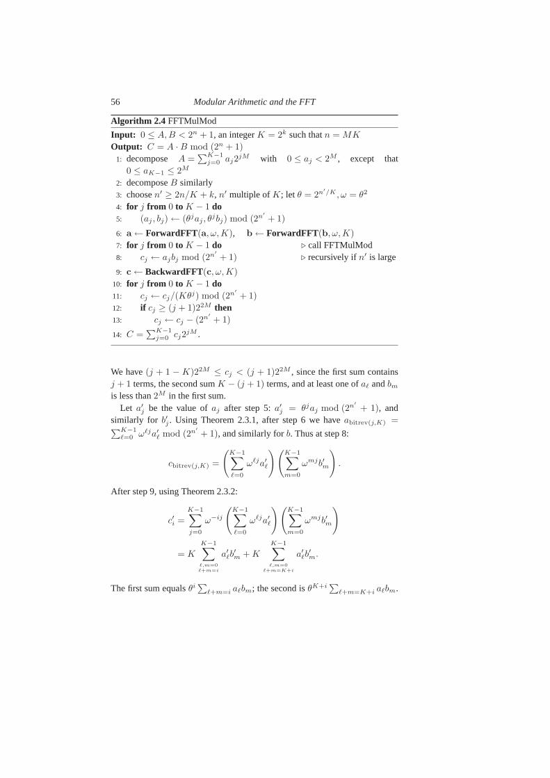
56 Modular Arithmetic and the FFT
Algorithm 2.4 FFTMulMod
Input: 0 ≤ A,B < 2n + 1, an integerK = 2k such thatn = MK
Output: C = A · B mod (2n + 1)
1: decompose A =∑K−1
j=0 aj2jM with 0 ≤ aj < 2M , except that
0 ≤ aK−1 ≤ 2M
2: decomposeB similarly3: choosen′ ≥ 2n/K + k, n′ multiple ofK; let θ = 2n′/K , ω = θ2
4: for j from 0 to K − 1 do5: (aj , bj) ← (θjaj , θ
jbj) mod (2n′
+ 1)
6: a ← ForwardFFT (a, ω,K), b ← ForwardFFT (b, ω,K)
7: for j from 0 to K − 1 do ⊲ call FFTMulMod8: cj ← ajbj mod (2n′
+ 1) ⊲ recursively ifn′ is large
9: c ← BackwardFFT(c, ω,K)
10: for j from 0 to K − 1 do11: cj ← cj/(Kθj) mod (2n′
+ 1)
12: if cj ≥ (j + 1)22M then13: cj ← cj − (2n′
+ 1)
14: C =∑K−1
j=0 cj2jM .
We have(j + 1 − K)22M ≤ cj < (j + 1)22M , since the first sum containsj + 1 terms, the second sumK − (j + 1) terms, and at least one ofaℓ andbm
is less than2M in the first sum.Let a′
j be the value ofaj after step 5:a′j = θjaj mod (2n′
+ 1), andsimilarly for b′j . Using Theorem 2.3.1, after step 6 we haveabitrev(j,K) =∑K−1
ℓ=0 ωℓja′ℓ mod (2n′
+ 1), and similarly forb. Thus at step 8:
cbitrev(j,K) =
(K−1∑
ℓ=0
ωℓja′ℓ
) (K−1∑
m=0
ωmjb′m
).
After step 9, using Theorem 2.3.2:
c′i =
K−1∑
j=0
ω−ij
(K−1∑
ℓ=0
ωℓja′ℓ
) (K−1∑
m=0
ωmjb′m
)
= K
K−1∑
ℓ,m=0
ℓ+m=i
a′ℓb
′m + K
K−1∑
ℓ,m=0
ℓ+m=K+i
a′ℓb
′m.
The first sum equalsθi∑
ℓ+m=i aℓbm; the second isθK+i∑
ℓ+m=K+i aℓbm.

2.3 The Fourier Transform 57
SinceθK = −1 mod (2n′
+ 1), after step 11 we have:
ci =
K−1∑
ℓ,m=0
ℓ+m=i
aℓbm −K−1∑
ℓ,m=0
ℓ+m=K+i
aℓbm mod (2n′
+ 1).
The correction at step 13 ensures thatci lies in the correct interval, as given byEqn. (2.2).
For the complexity analysis, assume thatK = Θ(√
n). Thus we haven′ =
Θ(√
n). Steps 1 and 2 costO(n); step 5 also costsO(n) (counting the cu-mulated cost for all values ofj). Step 6 costsO(K log K) times the costof one butterfly operation mod(2n′
+ 1), which is O(n′), thus a total ofO(Kn′ log K) = O(n log n). Step 8, using the same algorithm recursively,costsO(n′ log n′ log log n′) per value ofj by the induction hypothesis, giv-ing a total ofO(n log n log log n). The backward FFT costsO(n log n) too,and the final steps costO(n), giving a total cost ofO(n log n log log n). Thelog log n term is the depth of the recursion, each level reducingn to n′ =
O(√
n).
EXAMPLE : to multiply two integers modulo(21 048 576 +1), we can takeK =
210 = 1024, andn′ = 3072. We recursively compute1024 products modulo(23072 + 1). Alternatively, we can take the smaller valueK = 512, with 512
recursive products modulo(24608 + 1).REMARK 1: the “small” products at step 8 (mod(23072+1) or mod(24608+1)
in our example) can be performed by the same algorithm applied recursively,but at some point (determined by details of the implementation) it will be moreefficient to use a simpler algorithm, such as the classical orKaratsuba algo-rithm (see§1.3). In practice the depth of recursion is a small constant,typically1 or2. Thus, for practical purposes, thelog log n term can be regarded as a con-stant. For a theoretical way of avoiding thelog log n term, see the commentson Furer’s algorithm in§2.9.REMARK 2: if we replaceθ by 1 in Algorithm FFTMulMod , i.e., removestep 5, replace step 11 bycj ← cj/K mod (2n′
+1), and replace the conditionat step 12 bycj ≥ K·22M , then we computeC = A·B mod (2n−1) instead ofmod (2n +1). This is useful, for example, in McLaughlin’s algorithm (§2.4.3).
Algorithm FFTMulMod enables us to multiply two integers modulo(2n +
1) in O(n log n log log n) operations, for a suitablen and a corresponding FFTlengthK = 2k. Since we should haveK ≈ √
n andK must dividen, suitablevalues ofn are the integers with the low-order half of their bits zero; there isno shortage of such integers. To multiply two integers of at most n bits, wefirst choose a suitable bit sizem ≥ 2n. We consider the integers as residues
58 Modular Arithmetic and the FFT
modulo(2m + 1), then AlgorithmFFTMulMod gives their integer product.The resulting complexity isO(n log n log log n), sincem = O(n). In practicethelog log n term can be regarded as a constant; theoretically it can be replacedby an extremely slowly-growing function (see Remark1 above).
In this book, we sometimes implicitly assume thatn-bit integer multiplica-tion costs the same as three FFTs of length2n, since this is true if an FFT-basedalgorithm is used for multiplication. The constant “three”can be reduced ifsome of the FFTs can be precomputed and reused many times, forexample ifsome of the operands in the multiplications are fixed.
2.4 Modular Multiplication
Modular multiplication means computingA · B mod N , whereA andB areresidues moduloN . Of course, once the productC = A·B has been computed,it suffices to perform amodular reductionC mod N , which itself reduces toan integer division. The reader may ask why we did not cover this topic in§1.4. There are two reasons. First, the algorithms presentedbelow benefit fromsome precomputations involvingN , and are thus specific to the case whereseveral reductions are performed with the same modulus. Second, some algo-rithms avoid performing the full productC = A · B; one such example isMcLaughlin’s algorithm (§2.4.3).
Algorithms with precomputations include Barrett’s algorithm (§2.4.1), whichcomputes an approximation to the inverse of the modulus, thus trading divisionfor multiplication; Montgomery’s algorithm, which corresponds to Hensel’sdivision with remainder only (§1.4.8), and its subquadratic variant, which isthe LSB-variant of Barrett’s algorithm; and finally McLaughlin’s algorithm(§2.4.3). The cost of the precomputations is not taken into account: it is as-sumed to be negligible if many modular reductions are performed. However,we assume that the amount of precomputed data uses only linear, that isO(log N), space.
As usual, we assume that the modulusN hasn words in baseβ, thatA andB have at mostn words, and in some cases that they are fully reduced, i.e.,0 ≤ A,B < N .
2.4.1 Barrett’s Algorithm
Barrett’s algorithm is attractive when many divisions haveto be made withthe same divisor; this is the case when one performs computations modulo a
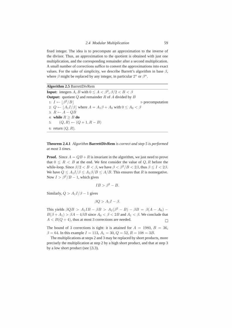
2.4 Modular Multiplication 59
fixed integer. The idea is to precompute an approximation to the inverse ofthe divisor. Thus, an approximation to the quotient is obtained with just onemultiplication, and the corresponding remainder after a second multiplication.A small number of corrections suffice to convert the approximations into exactvalues. For the sake of simplicity, we describe Barrett’s algorithm in baseβ,whereβ might be replaced by any integer, in particular2n or βn.
Algorithm 2.5 BarrettDivRem
Input: integersA, B with 0 ≤ A < β2, β/2 < B < β
Output: quotientQ and remainderR of A divided byB
1: I ← ⌊β2/B⌋ ⊲ precomputation2: Q ← ⌊A1I/β⌋ whereA = A1β + A0 with 0 ≤ A0 < β
3: R ← A − QB
4: while R ≥ B do5: (Q,R) ← (Q + 1, R − B)
6: return(Q,R).
Theorem 2.4.1 AlgorithmBarrettDivRem is correct and step 5 is performedat most3 times.
Proof. SinceA = QB +R is invariant in the algorithm, we just need to provethat 0 ≤ R < B at the end. We first consider the value ofQ,R before thewhile-loop. Sinceβ/2 < B < β, we haveβ < β2/B < 2β, thusβ ≤ I < 2β.We haveQ ≤ A1I/β ≤ A1β/B ≤ A/B. This ensures thatR is nonnegative.Now I > β2/B − 1, which gives
IB > β2 − B.
Similarly, Q > A1I/β − 1 gives
βQ > A1I − β.
This yieldsβQB > A1IB − βB > A1(β2 − B) − βB = β(A − A0) −
B(β + A1) > βA− 4βB sinceA0 < β < 2B andA1 < β. We conclude thatA < B(Q + 4), thus at most3 corrections are needed.
The bound of3 corrections is tight: it is attained forA = 1980, B = 36,β = 64. In this exampleI = 113, A1 = 30, Q = 52, R = 108 = 3B.
The multiplications at steps 2 and 3 may be replaced by short products, moreprecisely the multiplication at step 2 by a high short product, and that at step 3by a low short product (see§3.3).
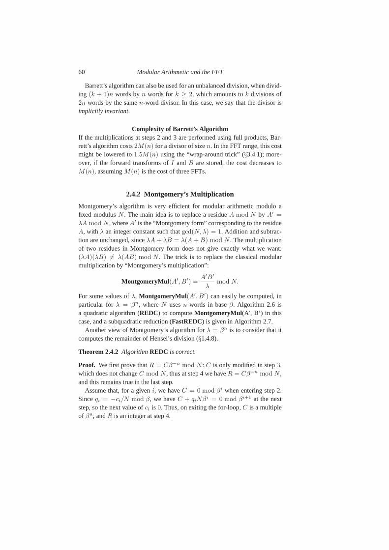
60 Modular Arithmetic and the FFT
Barrett’s algorithm can also be used for an unbalanced division, when divid-ing (k + 1)n words byn words fork ≥ 2, which amounts tok divisions of2n words by the samen-word divisor. In this case, we say that the divisor isimplicitly invariant.
Complexity of Barrett’s AlgorithmIf the multiplications at steps 2 and 3 are performed using full products, Bar-rett’s algorithm costs2M(n) for a divisor of sizen. In the FFT range, this costmight be lowered to1.5M(n) using the “wrap-around trick” (§3.4.1); more-over, if the forward transforms ofI andB are stored, the cost decreases toM(n), assumingM(n) is the cost of three FFTs.
2.4.2 Montgomery’s Multiplication
Montgomery’s algorithm is very efficient for modular arithmetic modulo afixed modulusN . The main idea is to replace a residueA mod N by A′ =
λA mod N , whereA′ is the “Montgomery form” corresponding to the residueA, with λ an integer constant such thatgcd(N,λ) = 1. Addition and subtrac-tion are unchanged, sinceλA + λB = λ(A + B) mod N . The multiplicationof two residues in Montgomery form does not give exactly whatwe want:(λA)(λB) 6= λ(AB) mod N . The trick is to replace the classical modularmultiplication by “Montgomery’s multiplication”:
MontgomeryMul (A′, B′) =A′B′
λmod N.
For some values ofλ, MontgomeryMul (A′, B′) can easily be computed, inparticular forλ = βn, whereN usesn words in baseβ. Algorithm 2.6 isa quadratic algorithm (REDC) to computeMontgomeryMul (A’, B’) in thiscase, and a subquadratic reduction (FastREDC) is given in Algorithm 2.7.
Another view of Montgomery’s algorithm forλ = βn is to consider that itcomputes the remainder of Hensel’s division (§1.4.8).
Theorem 2.4.2 AlgorithmREDC is correct.
Proof. We first prove thatR = Cβ−n mod N : C is only modified in step 3,which does not changeC mod N , thus at step 4 we haveR = Cβ−n mod N ,and this remains true in the last step.
Assume that, for a giveni, we haveC = 0 mod βi when entering step 2.Sinceqi = −ci/N mod β, we haveC + qiNβi = 0 mod βi+1 at the nextstep, so the next value ofci is 0. Thus, on exiting the for-loop,C is a multipleof βn, andR is an integer at step 4.
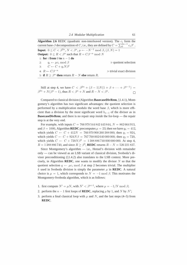
2.4 Modular Multiplication 61
Algorithm 2.6 REDC (quadratic non-interleaved version). Theci form thecurrent base-β decomposition ofC, i.e., they are defined byC =
∑2n−10 ciβ
i .
Input: 0 ≤ C < β2n, N < βn, µ ← −N−1 mod β, (β,N) = 1
Output: 0 ≤ R < βn such thatR = Cβ−n mod N
1: for i from 0 to n − 1 do2: qi ← µci mod β ⊲ quotient selection3: C ← C + qiNβi
4: R ← Cβ−n ⊲ trivial exact division5: if R ≥ βn then returnR − N elsereturnR.
Still at step 4, we haveC < β2n + (β − 1)N(1 + β + · · · + βn−1) =
β2n + N(βn − 1), thusR < βn + N andR − N < βn.
Compared to classical division (AlgorithmBasecaseDivRem, §1.4.1), Mont-gomery’s algorithm has two significant advantages: the quotient selection isperformed by a multiplication modulo the word baseβ, which is more effi-cient than a division by the most significant wordbn−1 of the divisor as inBasecaseDivRem; and there is no repair stepinsidethe for-loop — the repairstep is at the very end.
For example, with inputsC = 766 970 544 842 443 844, N = 862 664 913,andβ = 1000, AlgorithmREDC precomputesµ = 23; then we haveq0 = 412,which yieldsC ← C + 412N = 766 970 900 260 388 000; then q1 = 924,which yieldsC ← C + 924Nβ = 767 768 002 640 000 000; thenq2 = 720,which yieldsC ← C + 720Nβ2 = 1388 886 740 000 000 000. At step 4,R = 1388 886 740, and sinceR ≥ β3, REDC returnsR − N = 526 221 827.
Since Montgomery’s algorithm — i.e., Hensel’s division with remainderonly — can be viewed as an LSB variant of classical division, Svoboda’s di-visor preconditioning (§1.4.2) also translates to the LSB context. More pre-cisely, in AlgorithmREDC, one wants to modify the divisorN so that thequotient selectionq ← µci mod β at step 2 becomes trivial. The multiplierk used in Svoboda division is simply the parameterµ in REDC. A naturalchoice isµ = 1, which corresponds toN = −1 mod β. This motivates theMontgomery-Svoboda algorithm, which is as follows:
1. first computeN ′ = µN , with N ′ < βn+1, whereµ = −1/N mod β;
2. perform then − 1 first loops ofREDC, replacingµ by 1, andN by N ′;
3. perform a final classical loop withµ andN , and the last steps (4–5) fromREDC.
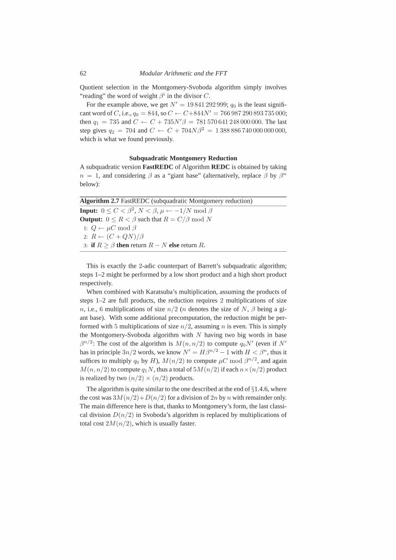
62 Modular Arithmetic and the FFT
Quotient selection in the Montgomery-Svoboda algorithm simply involves“reading” the word of weightβi in the divisorC.
For the example above, we getN ′ = 19 841 292 999; q0 is the least signifi-cant word ofC, i.e.,q0 = 844, soC ← C+844N ′ = 766 987 290 893 735 000;thenq1 = 735 andC ← C + 735N ′β = 781 570 641 248 000 000. The laststep givesq2 = 704 andC ← C + 704Nβ2 = 1388 886 740 000 000 000,which is what we found previously.
Subquadratic Montgomery ReductionA subquadratic versionFastREDCof Algorithm REDC is obtained by takingn = 1, and consideringβ as a “giant base” (alternatively, replaceβ by βn
below):
Algorithm 2.7 FastREDC (subquadratic Montgomery reduction)
Input: 0 ≤ C < β2, N < β, µ ← −1/N mod β
Output: 0 ≤ R < β such thatR = C/β mod N
1: Q ← µC mod β
2: R ← (C + QN)/β
3: if R ≥ β then returnR − N elsereturnR.
This is exactly the2-adic counterpart of Barrett’s subquadratic algorithm;steps 1–2 might be performed by a low short product and a high short productrespectively.
When combined with Karatsuba’s multiplication, assuming the products ofsteps 1–2 are full products, the reduction requires2 multiplications of sizen, i.e., 6 multiplications of sizen/2 (n denotes the size ofN , β being a gi-ant base). With some additional precomputation, the reduction might be per-formed with5 multiplications of sizen/2, assumingn is even. This is simplythe Montgomery-Svoboda algorithm withN having two big words in baseβn/2: The cost of the algorithm isM(n, n/2) to computeq0N
′ (even if N ′
has in principle3n/2 words, we knowN ′ = Hβn/2 − 1 with H < βn, thus itsuffices to multiplyq0 by H), M(n/2) to computeµC mod βn/2, and againM(n, n/2) to computeq1N , thus a total of5M(n/2) if eachn×(n/2) productis realized by two(n/2) × (n/2) products.
The algorithm is quite similar to the one described at the endof §1.4.6, wherethe cost was3M(n/2)+D(n/2) for a division of2n byn with remainder only.The main difference here is that, thanks to Montgomery’s form, the last classi-cal divisionD(n/2) in Svoboda’s algorithm is replaced by multiplications oftotal cost2M(n/2), which is usually faster.
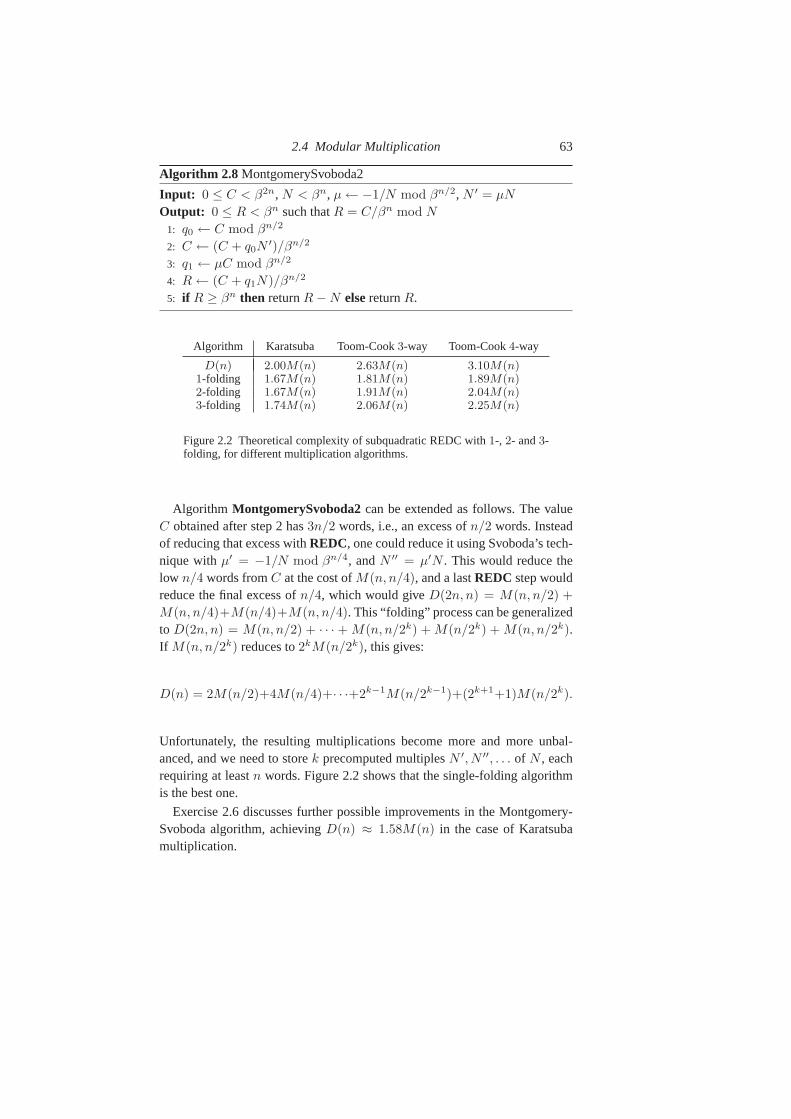
2.4 Modular Multiplication 63
Algorithm 2.8 MontgomerySvoboda2
Input: 0 ≤ C < β2n, N < βn, µ ← −1/N mod βn/2, N ′ = µN
Output: 0 ≤ R < βn such thatR = C/βn mod N
1: q0 ← C mod βn/2
2: C ← (C + q0N′)/βn/2
3: q1 ← µC mod βn/2
4: R ← (C + q1N)/βn/2
5: if R ≥ βn then returnR − N elsereturnR.
Algorithm Karatsuba Toom-Cook3-way Toom-Cook4-way
D(n) 2.00M(n) 2.63M(n) 3.10M(n)1-folding 1.67M(n) 1.81M(n) 1.89M(n)2-folding 1.67M(n) 1.91M(n) 2.04M(n)3-folding 1.74M(n) 2.06M(n) 2.25M(n)
Figure 2.2 Theoretical complexity of subquadratic REDC with1-, 2- and3-folding, for different multiplication algorithms.
Algorithm MontgomerySvoboda2can be extended as follows. The valueC obtained after step 2 has3n/2 words, i.e., an excess ofn/2 words. Insteadof reducing that excess withREDC, one could reduce it using Svoboda’s tech-nique withµ′ = −1/N mod βn/4, andN ′′ = µ′N . This would reduce thelow n/4 words fromC at the cost ofM(n, n/4), and a lastREDC step wouldreduce the final excess ofn/4, which would giveD(2n, n) = M(n, n/2) +
M(n, n/4)+M(n/4)+M(n, n/4). This “folding” process can be generalizedto D(2n, n) = M(n, n/2) + · · · + M(n, n/2k) + M(n/2k) + M(n, n/2k).If M(n, n/2k) reduces to2kM(n/2k), this gives:
D(n) = 2M(n/2)+4M(n/4)+· · ·+2k−1M(n/2k−1)+(2k+1+1)M(n/2k).
Unfortunately, the resulting multiplications become moreand more unbal-anced, and we need to storek precomputed multiplesN ′, N ′′, . . . of N , eachrequiring at leastn words. Figure 2.2 shows that the single-folding algorithmis the best one.
Exercise 2.6 discusses further possible improvements in the Montgomery-Svoboda algorithm, achievingD(n) ≈ 1.58M(n) in the case of Karatsubamultiplication.
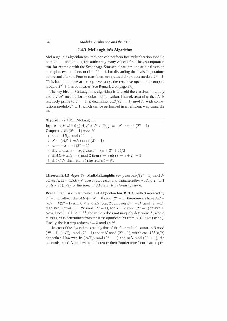
64 Modular Arithmetic and the FFT
2.4.3 McLaughlin’s Algorithm
McLaughlin’s algorithm assumes one can perform fast multiplication moduloboth2n − 1 and2n + 1, for sufficiently many values ofn. This assumption istrue for example with the Schonhage-Strassen algorithm: the original versionmultiplies two numbers modulo2n + 1, but discarding the “twist” operationsbefore and after the Fourier transforms computes their product modulo2n −1.(This has to be done at the top level only: the recursive operations computemodulo2n′
+ 1 in both cases. See Remark 2 on page 57.)The key idea in McLaughlin’s algorithm is to avoid the classical “multiply
and divide” method for modular multiplication. Instead, assuming thatN isrelatively prime to2n − 1, it determinesAB/(2n − 1) mod N with convo-lutions modulo2n ± 1, which can be performed in an efficient way using theFFT.
Algorithm 2.9 MultMcLaughlin
Input: A,B with 0 ≤ A,B < N < 2n, µ = −N−1 mod (2n − 1)
Output: AB/(2n − 1) mod N
1: m ← ABµ mod (2n − 1)
2: S ← (AB + mN) mod (2n + 1)
3: w ← −S mod (2n + 1)
4: if 2|w then s ← w/2 elses ← (w + 2n + 1)/2
5: if AB + mN = s mod 2 then t ← s elset ← s + 2n + 1
6: if t < N then returnt elsereturnt − N .
Theorem 2.4.3 AlgorithmMultMcLaughlin computesAB/(2n−1) mod N
correctly, in∼ 1.5M(n) operations, assuming multiplication modulo2n ± 1
costs∼M(n/2), or the same as3 Fourier transforms of sizen.
Proof. Step 1 is similar to step 1 of AlgorithmFastREDC, with β replaced by2n −1. It follows thatAB +mN = 0 mod (2n −1), therefore we haveAB +
mN = k(2n−1) with 0 ≤ k < 2N . Step 2 computesS = −2k mod (2n+1),then step 3 givesw = 2k mod (2n + 1), ands = k mod (2n + 1) in step 4.Now, since0 ≤ k < 2n+1, the values does not uniquely determinek, whosemissing bit is determined from the least significant bit fromAB+mN (step 5).Finally, the last step reducest = k moduloN .
The cost of the algorithm is mainly that of the four multiplicationsAB mod
(2n ±1), (AB)µ mod (2n −1) andmN mod (2n +1), which cost4M(n/2)
altogether. However, in(AB)µ mod (2n − 1) and mN mod (2n + 1), theoperandsµ andN are invariant, therefore their Fourier transforms can be pre-
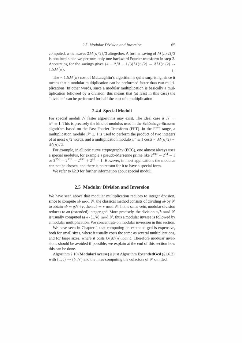
2.5 Modular Division and Inversion 65
computed, which saves2M(n/2)/3 altogether. A further saving ofM(n/2)/3
is obtained since we perform only one backward Fourier transform in step 2.Accounting for the savings gives(4 − 2/3 − 1/3)M(n/2) = 3M(n/2) ∼1.5M(n).
The∼1.5M(n) cost of McLaughlin’s algorithm is quite surprising, since itmeans that a modular multiplication can be performed fasterthan two multi-plications. In other words, since a modular multiplicationis basically a mul-tiplication followed by a division, this means that (at least in this case) the“division” can be performed for half the cost of a multiplication!
2.4.4 Special Moduli
For special moduliN faster algorithms may exist. The ideal case isN =
βn ± 1. This is precisely the kind of modulus used in the Schonhage-Strassenalgorithm based on the Fast Fourier Transform (FFT). In the FFT range, amultiplication moduloβn ± 1 is used to perform the product of two integersof at mostn/2 words, and a multiplication moduloβn ± 1 costs∼M(n/2) ∼M(n)/2.
For example, in elliptic curve cryptography (ECC), one almost always usesa special modulus, for example a pseudo-Mersenne prime like2192 − 264 − 1
or 2256 − 2224 + 2192 + 296 − 1. However, in most applications the moduluscan not be chosen, and there is no reason for it to have a special form.
We refer to§2.9 for further information about special moduli.
2.5 Modular Division and Inversion
We have seen above that modular multiplication reduces to integer division,since to computeab mod N , the classical method consists of dividingab by N
to obtainab = qN+r, thenab = r mod N . In the same vein, modular divisionreduces to an (extended) integer gcd. More precisely, the divisiona/b mod N
is usually computed asa · (1/b) mod N , thus a modular inverse is followed bya modular multiplication. We concentrate on modular inversion in this section.
We have seen in Chapter 1 that computing an extended gcd is expensive,both for small sizes, where it usually costs the same as several multiplications,and for large sizes, where it costsO(M(n) log n). Therefore modular inver-sions should be avoided if possible; we explain at the end of this section howthis can be done.
Algorithm 2.10 (ModularInverse) is just AlgorithmExtendedGcd(§1.6.2),with (a, b) → (b,N) and the lines computing the cofactors ofN omitted.
66 Modular Arithmetic and the FFT
Algorithm 2.10 ModularInverseInput: integersb andN , b prime toN
Output: integeru = 1/b mod N
(u,w) ← (1, 0), c ← N
while c 6= 0 do(q, r) ← DivRem(b, c)
(b, c) ← (c, r)
(u,w) ← (w, u − qw)
returnu.
Algorithm ModularInverse is the naive version of modular inversion, withcomplexity O(n2) if N takes n words in baseβ. The subquadraticO(M(n) log n) algorithm is based on theHalfBinaryGcd algorithm (§1.6.3).
When the modulusN has a special form, faster algorithms may exist. Inparticular forN = pk, O(M(n)) algorithms exist, based on Hensel lifting,which can be seen as thep-adic variant of Newton’s method (§4.2). To compute1/b mod N , we use ap-adic version of the iteration (4.5):
xj+1 = xj + xj(1 − bxj) mod pk. (2.3)
Assumexj approximates1/b to “p-adic precision”ℓ, i.e.,bxj = 1 + εpℓ, andk = 2ℓ. Then, modulopk: bxj+1 = bxj(2 − bxj) = (1 + εpℓ)(1 − εpℓ) =
1− ε2p2ℓ. Thereforexj+1 approximates1/b to double precision (in thep-adicsense).
As an example, assume one wants to compute the inverse of an odd integerbmodulo232. The initial approximationx0 = 1 satisfiesx0 = 1/b mod 2, thusfive iterations are enough. The first iteration isx1 ← x0+x0(1−bx0) mod 22,which simplifies tox1 ← 2 − b mod 4 sincex0 = 1. Now whetherb =
1 mod 4 or b = 3 mod 4, we have2−b = b mod 4, thus one can immediatelystart the second iteration withx1 = b implicit:
x2 ← b(2 − b2) mod 24, x3 ← x2(2 − bx2) mod 28,
x4 ← x3(2 − bx3) mod 216, x5 ← x4(2 − bx4) mod 232.
Consider for exampleb = 17. The above algorithm yieldsx2 = 1, x3 = 241,x4 = 61 681 andx5 = 4042 322 161. Of course, any computation modpℓ
might be computed modulopk for k ≥ ℓ. In particular, all the above compu-tations might be performed modulo232. On a32-bit computer, arithmetic onbasic integer types is usually performed modulo232, thus the reduction comes

2.5 Modular Division and Inversion 67
for free, and one can write in the C language (usingunsigned variables andthe same variablex for x2, . . . , x5):
x = b * (2-b * b); x * = 2-b * x; x * = 2-b * x; x * = 2-b * x;
Another way to perform modular division when the modulus hasa specialform is Hensel’s division (§1.4.8). For a modulusN = βn, given two integersA,B, we computeQ andR such that
A = QB + Rβn.
Therefore we haveA/B = Q mod βn. While Montgomery’s modular mul-tiplication only computes the remainderR of Hensel’s division, modular di-vision computes the quotientQ, thus Hensel’s division plays a central role inmodular arithmetic moduloβn.
2.5.1 Several Inversions at Once
A modular inversion, which reduces to an extended gcd (§1.6.2), is usuallymuch more expensive than a multiplication. This is true not only in the FFTrange, where a gcd takes timeΘ(M(n) log n), but also for smaller numbers.When several inversions are to be performed modulo the same number, Algo-rithm MultipleInversion is usually faster.
Algorithm 2.11 MultipleInversionInput: 0 < x1, . . . , xk < N
Output: y1 = 1/x1 mod N, . . . , yk = 1/xk mod N
1: z1 ← x1
2: for i from 2 to k do3: zi ← zi−1xi mod N
4: q ← 1/zk mod N
5: for i from k downto 2 do6: yi ← qzi−1 mod N
7: q ← qxi mod N
8: y1 ← q.
Theorem 2.5.1 AlgorithmMultipleInversion is correct.
Proof. We havezi = x1x2 . . . xi mod N , thus at the beginning of step 6 for agiveni, q = (x1 . . . xi)
−1 mod N , which indeed givesyi = 1/xi mod N .
68 Modular Arithmetic and the FFT
This algorithm uses only one modular inversion (step 4), and3(k−1) modularmultiplications. Thus it is faster thank inversions when a modular inversion ismore than three times as expensive as a product. Figure 2.3 shows a recursivevariant of the algorithm, with the same number of modular multiplications: onefor each internal node when going up the (product) tree, and two for each in-ternal node when going down the (remainder) tree. The recursive variant mightbe performed in parallel inO(log k) operations usingO(k/ log k) processors.
¡¡
¡¡
¡
@@
@@
@¡
¡¡
@@@
¡¡¡
@@@
1/(x1x2x3x4)
1/(x1x2) 1/(x3x4)
1/x1 1/x2 1/x3 1/x4
Figure 2.3 A recursive variant of AlgorithmMultipleInversion . First goup the tree, buildingx1x2 mod N from x1 and x2 in the left branch,x3x4 mod N in the right branch, andx1x2x3x4 mod N at the root of thetree. Then invert the root of the tree. Finally go down the tree, multiplying1/(x1x2x3x4) by the stored valuex3x4 to get1/(x1x2), and so on.
A dual case is when there are several moduli but the number to invert isfixed. Say we want to compute1/x mod N1, . . . , 1/x mod Nk. We illustratea possible algorithm in the casek = 4. First computeN = N1 . . . Nk usinga product tree like that in Figure 2.3, for example first compute N1N2 andN3N4, then multiply both to getN = (N1N2)(N3N4). Then computey =
1/x mod N , and go down the tree, while reducing the residue at each node. Inour example we computez = y mod (N1N2) in the left branch, thenz mod
N1 yields1/x mod N1. An important difference between this algorithm andthe algorithm illustrated in Figure 2.3 is that here, the numbers grow whilegoing up the tree. Thus, depending on the sizes ofx and theNj , this algorithmmight be of theoretical interest only.
2.6 Modular Exponentiation
Modular exponentiation is the most time-consuming mathematical operationin several cryptographic algorithms. The well-known RSA public-key cryp-tosystem is based on the fact that computing
c = ae mod N (2.4)
2.6 Modular Exponentiation 69
is relatively easy, but recoveringa from c, e andN is difficult whenN hasat least two (unknown) large prime factors. The discrete logarithm problem issimilar: herec, a andN are given, and one looks fore satisfying Eqn. (2.4).In this case the problem is difficult whenN has at least one large prime factor(for example,N could be prime). The discrete logarithm problem is the basisof the El Gamal cryptosystem, and a closely related problem is the basis of theDiffie-Hellman key exchange protocol.
When the exponente is fixed (or known to be small), an optimal sequenceof squarings and multiplications might be computed in advance. This is relatedto the classicaladdition chainproblem: What is the smallest chain of additionsto reach the integere, starting from1? For example, ife = 15, a possible chainis:
1, 1 + 1 = 2, 1 + 2 = 3, 1 + 3 = 4, 3 + 4 = 7, 7 + 7 = 14, 1 + 14 = 15.
The length of a chain is defined to be the number of additions needed to com-pute it (the above chain has length6). An addition chain readily translates to amultiplication chain:
a, a ·a = a2, a ·a2 = a3, a ·a3 = a4, a3 ·a4 = a7, a7 ·a7 = a14, a ·a14 = a15.
A shorter chain fore = 15 is:
1, 1 + 1 = 2, 1 + 2 = 3, 2 + 3 = 5, 5 + 5 = 10, 5 + 10 = 15.
This chain is the shortest possible fore = 15, so we writeσ(15) = 5, where ingeneralσ(e) denotes the length of the shortest addition chain fore. In the casewheree is small, and an addition chain of shortest lengthσ(e) is known fore,computingae mod N may be performed inσ(e) modular multiplications.
Whene is large and(a,N) = 1, thene might be reduced moduloφ(N),whereφ(N) is Euler’s totient function, i.e., the number of integers in[1, N ]
which are relatively prime toN . This is becauseaφ(N) = 1 mod N whenever(a,N) = 1 (Fermat’s little theorem).
Sinceφ(N) is a multiplicative function, it is easy to computeφ(N) if weknow the prime factorisation ofN . For example,
φ(1001) = φ(7 · 11 · 13) = (7 − 1)(11 − 1)(13 − 1) = 720,
and2009 = 569 mod 720, so172009 = 17569 mod 1001.Assume now thate is smaller thanφ(N). Since a lower bound on the length
σ(e) of the addition chain fore is lg e, this yields a lower bound(lg e)M(n)
for modular exponentiation, wheren is the size ofN . Whene is of sizek, amodular exponentiation costsO(kM(n)). Fork = n, the costO(nM(n)) ofmodular exponentiation is much more than the cost of operations considered in
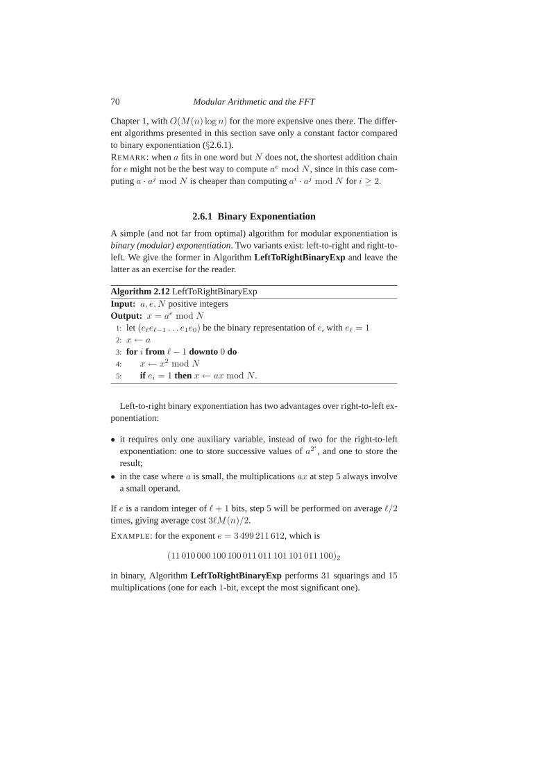
70 Modular Arithmetic and the FFT
Chapter 1, withO(M(n) log n) for the more expensive ones there. The differ-ent algorithms presented in this section save only a constant factor comparedto binary exponentiation (§2.6.1).REMARK : whena fits in one word butN does not, the shortest addition chainfor e might not be the best way to computeae mod N , since in this case com-putinga · aj mod N is cheaper than computingai · aj mod N for i ≥ 2.
2.6.1 Binary Exponentiation
A simple (and not far from optimal) algorithm for modular exponentiation isbinary (modular) exponentiation. Two variants exist: left-to-right and right-to-left. We give the former in AlgorithmLeftToRightBinaryExp and leave thelatter as an exercise for the reader.
Algorithm 2.12 LeftToRightBinaryExpInput: a, e,N positive integersOutput: x = ae mod N
1: let (eℓeℓ−1 . . . e1e0) be the binary representation ofe, with eℓ = 1
2: x ← a
3: for i from ℓ − 1 downto 0 do4: x ← x2 mod N
5: if ei = 1 then x ← ax mod N .
Left-to-right binary exponentiation has two advantages over right-to-left ex-ponentiation:
• it requires only one auxiliary variable, instead of two for the right-to-leftexponentiation: one to store successive values ofa2i
, and one to store theresult;
• in the case wherea is small, the multiplicationsax at step 5 always involvea small operand.
If e is a random integer ofℓ + 1 bits, step 5 will be performed on averageℓ/2
times, giving average cost3ℓM(n)/2.
EXAMPLE : for the exponente = 3499 211 612, which is
(11 010 000 100 100 011 011 101 101 011 100)2
in binary, AlgorithmLeftToRightBinaryExp performs31 squarings and15
multiplications (one for each1-bit, except the most significant one).
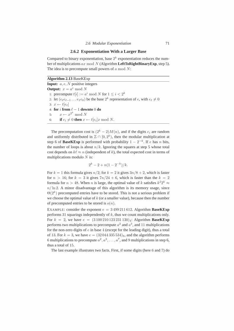
2.6 Modular Exponentiation 71
2.6.2 Exponentiation With a Larger Base
Compared to binary exponentiation, base2k exponentiation reduces the num-ber of multiplicationsax mod N (AlgorithmLeftToRightBinaryExp , step 5).The idea is to precompute small powers ofa mod N :
Algorithm 2.13 BaseKExpInput: a, e,N positive integersOutput: x = ae mod N
1: precomputet[i] := ai mod N for 1 ≤ i < 2k
2: let (eℓeℓ−1 . . . e1e0) be the base2k representation ofe, with eℓ 6= 0
3: x ← t[eℓ]
4: for i from ℓ − 1 downto 0 do5: x ← x2k
mod N
6: if ei 6= 0 then x ← t[ei]x mod N .
The precomputation cost is(2k − 2)M(n), and if the digitsei are randomand uniformly distributed inZ ∩ [0, 2k), then the modular multiplication atstep 6 ofBaseKExp is performed with probability1 − 2−k. If e hasn bits,the number of loops is aboutn/k. Ignoring the squares at step 5 whose totalcost depends onkℓ ≈ n (independent ofk), the total expected cost in terms ofmultiplications moduloN is:
2k − 2 + n(1 − 2−k)/k.
Fork = 1 this formula givesn/2; for k = 2 it gives3n/8 + 2, which is fasterfor n > 16; for k = 3 it gives 7n/24 + 6, which is faster than thek = 2
formula forn > 48. Whenn is large, the optimal value ofk satisfiesk22k ≈n/ ln 2. A minor disadvantage of this algorithm is its memory usage,sinceΘ(2k) precomputed entries have to be stored. This is not a serious problem ifwe choose the optimal value ofk (or a smaller value), because then the numberof precomputed entries to be stored iso(n).
EXAMPLE : consider the exponente = 3499 211 612. Algorithm BaseKExpperforms31 squarings independently ofk, thus we count multiplications only.For k = 2, we havee = (3 100 210 123 231 130)4: Algorithm BaseKExpperforms two multiplications to precomputea2 anda3, and11 multiplicationsfor the non-zero digits ofe in base4 (except for the leading digit), thus a totalof 13. Fork = 3, we havee = (32 044 335 534)8, and the algorithm performs6 multiplications to precomputea2, a3, . . . , a7, and9 multiplications in step 6,thus a total of15.
The last example illustrates two facts. First, if some digits (here6 and7) do
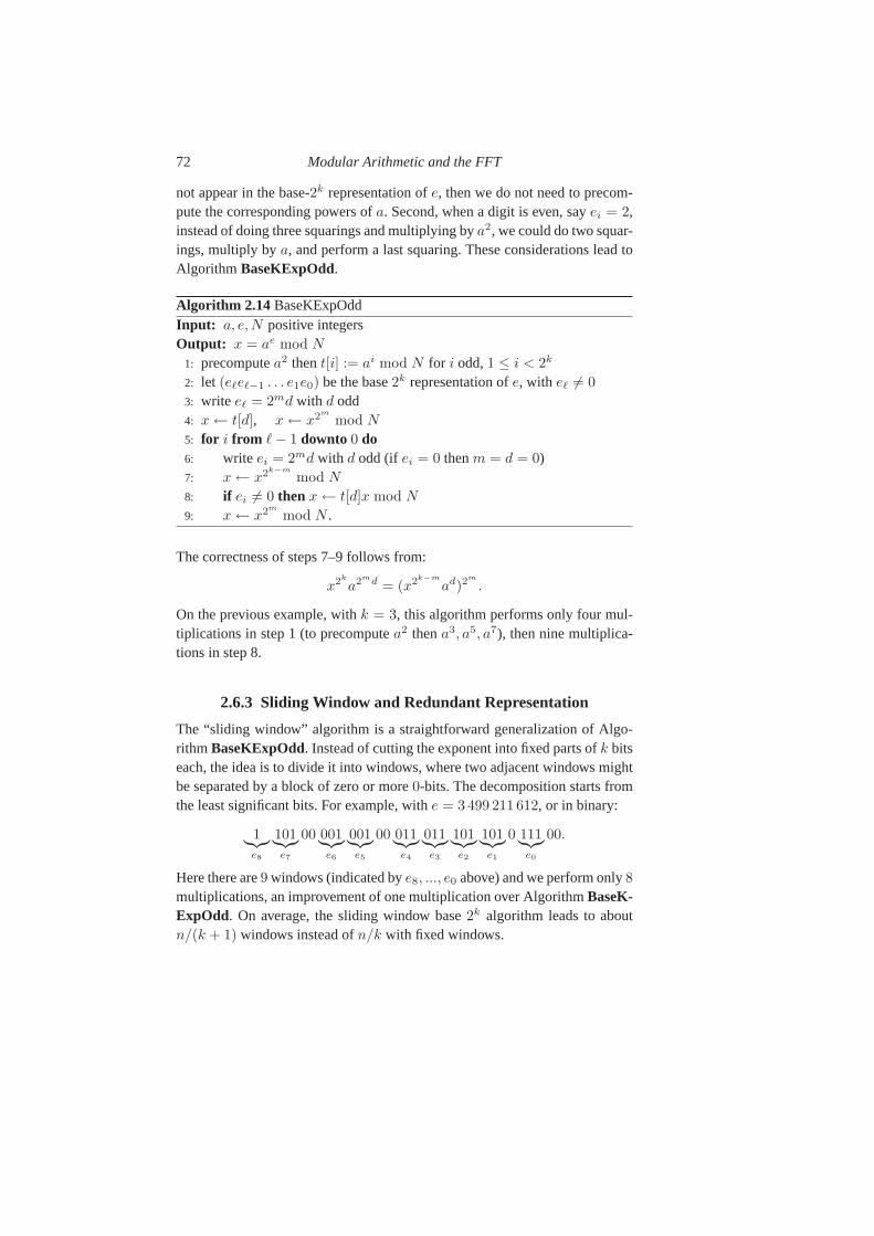
72 Modular Arithmetic and the FFT
not appear in the base-2k representation ofe, then we do not need to precom-pute the corresponding powers ofa. Second, when a digit is even, sayei = 2,instead of doing three squarings and multiplying bya2, we could do two squar-ings, multiply bya, and perform a last squaring. These considerations lead toAlgorithm BaseKExpOdd.
Algorithm 2.14 BaseKExpOddInput: a, e,N positive integersOutput: x = ae mod N
1: precomputea2 thent[i] := ai mod N for i odd,1 ≤ i < 2k
2: let (eℓeℓ−1 . . . e1e0) be the base2k representation ofe, with eℓ 6= 0
3: write eℓ = 2md with d odd4: x ← t[d], x ← x2m
mod N
5: for i from ℓ − 1 downto 0 do6: write ei = 2md with d odd (if ei = 0 thenm = d = 0)7: x ← x2k−m
mod N
8: if ei 6= 0 then x ← t[d]x mod N
9: x ← x2m
mod N .
The correctness of steps 7–9 follows from:
x2k
a2md = (x2k−m
ad)2m
.
On the previous example, withk = 3, this algorithm performs only four mul-tiplications in step 1 (to precomputea2 thena3, a5, a7), then nine multiplica-tions in step 8.
2.6.3 Sliding Window and Redundant Representation
The “sliding window” algorithm is a straightforward generalization of Algo-rithm BaseKExpOdd. Instead of cutting the exponent into fixed parts ofk bitseach, the idea is to divide it into windows, where two adjacent windows mightbe separated by a block of zero or more0-bits. The decomposition starts fromthe least significant bits. For example, withe = 3499 211 612, or in binary:
1︸︷︷︸e8
101︸︷︷︸e7
00 001︸︷︷︸e6
001︸︷︷︸e5
00 011︸︷︷︸e4
011︸︷︷︸e3
101︸︷︷︸e2
101︸︷︷︸e1
0 111︸︷︷︸e0
00.
Here there are9 windows (indicated bye8, ..., e0 above) and we perform only8multiplications, an improvement of one multiplication over Algorithm BaseK-ExpOdd. On average, the sliding window base2k algorithm leads to aboutn/(k + 1) windows instead ofn/k with fixed windows.
2.7 Chinese Remainder Theorem 73
Another improvement may be feasible when division is feasible (and cheap)in the underlying group. For example, if we encounter three consecutive ones,say111, in the binary representation ofe, we may replace some bits by−1,denoted by1, as in1001. We have thus replaced three multiplications by onemultiplication and one division, in other wordsx7 = x8 ·x−1. For our runningexample, this gives:
e = 11 010 000 100 100 100 100 010 010 100 100,
which has only10 non-zero digits, apart from the leading one, instead of15
with bits0 and1 only. The redundant representation with bits0, 1, 1 is calledthe Booth representation. It is a special case of theAvizienis signed-digit re-dundant representation. Signed-digit representations exist in any base.
For simplicity we have not distinguished between the cost ofmultiplica-tion and the cost of squaring (when the two operands in the multiplication areknown to be equal), but this distinction is significant in some applications (e.g.,elliptic curve cryptography). Note that, when the underlying group operationis denoted by addition rather than multiplication, as is usually the case forabelian groups (such as groups defined over elliptic curves), then the discus-sion above applies with “multiplication” replaced by “addition”, “division” by“subtraction”, and “squaring” by “doubling”.
2.7 Chinese Remainder Theorem
In applications where integer or rational results are expected, it is often worth-while to use a “residue number system” (as in§2.1.3) and perform all compu-tations modulo several small primes (or pairwise coprime integers). The finalresult can then be recovered via the Chinese Remainder Theorem (CRT). Forsuch applications, it is important to have fast conversion routines from integerto modular representation, and vice versa.
The integer to modular conversion problem is the following:given an integerx, and several pairwise coprime modulimi, 1 ≤ i ≤ k, how to efficientlycomputexi = x mod mi, for 1 ≤ i ≤ k? This is the remainder tree problem ofAlgorithm IntegerToRNS, which is also discussed in§2.5.1 and Exercise 1.35.
If all moduli mi have the same size, and if the sizen of x is comparable tothat of the productm1m2 · · ·mk, the costT (k) of Algorithm IntegerToRNSsatisfies the recurrenceT (n) = 2D(n/2) + 2T (n/2), which yieldsT (n) =
O(M(n) log n). Such a conversion is therefore more expensive than a multipli-cation or division, and is comparable in complexity terms toa base conversionor a gcd.
74 Modular Arithmetic and the FFT
Algorithm 2.15 IntegerToRNSInput: integerx, modulim1,m2, . . . ,mk pairwise coprime,k ≥ 1
Output: xi = x mod mi for 1 ≤ i ≤ k
1: if k ≤ 2 then2: returnx1 = x mod m1, . . . ,xk = x mod mk
3: ℓ ← ⌊k/2⌋4: M1 ← m1m2 · · ·mℓ, M2 ← mℓ+1 · · ·mk ⊲ might be precomputed5: x1, . . . , xℓ ← IntegerToRNS(x mod M1,m1, . . . ,mℓ)
6: xℓ+1, . . . , xk ← IntegerToRNS(x mod M2,mℓ+1, . . . ,mk).
The converseCRT reconstructionproblem is the following: given thexi,how to efficiently reconstruct the unique integerx, 0 ≤ x < m1m2 · · ·mk,such thatx = xi mod mi, for 1 ≤ i ≤ k? AlgorithmRNSToIntegerperformsthat conversion, where the valuesu, v at step 7 might be precomputed if severalconversions are made with the same moduli, and step 11 ensures that the finalresultx lies in the interval[0,M1M2).
Algorithm 2.16 RNSToIntegerInput: residuesxi, 0 ≤ xi < mi for 1 ≤ i ≤ k, mi pairwise coprimeOutput: 0 ≤ x < m1m2 · · ·mk with x = xi mod mi
1: if k = 1 then2: returnx1
3: ℓ ← ⌊k/2⌋4: M1 ← m1m2 · · ·mℓ, M2 ← mℓ+1 · · ·mk ⊲ might be precomputed5: X1 ← RNSToInteger([x1, . . . , xℓ], [m1, . . . ,mℓ])
6: X2 ← RNSToInteger([xℓ+1, . . . , xk], [mℓ+1, . . . ,mk])
7: computeu, v such thatuM1 + vM2 = 1 ⊲ might be precomputed8: λ1 ← uX2 mod M2, λ2 ← vX1 mod M1
9: x ← λ1M1 + λ2M2
10: if x ≥ M1M2 then11: x ← x − M1M2.
To see that AlgorithmRNSToInteger is correct, consider an integeri, 1 ≤i ≤ k, and show thatx = xi mod mi. If k = 1, it is trivial. Assumek ≥ 2,and without loss of generality1 ≤ i ≤ ℓ. SinceM1 is a multiple ofmi, wehavex mod mi = (x mod M1) mod mi, where
x mod M1 = λ2M2 mod M1 = vX1M2 mod M1 = X1 mod M1,
and the result follows from the induction hypothesis thatX1 = xi mod mi.
2.8 Exercises 75
Like IntegerToRNS, Algorithm RNSToInteger costsO(M(n) log n) forM = m1m2 · · ·mk of sizen, assuming that themi are of equal sizes.
The CRT reconstruction problem is analogous to the Lagrangepolynomialinterpolation problem: find a polynomial of minimal degree interpolating givenvaluesxi atk pointsmi.
A “flat” variant of the explicit Chinese remainder reconstruction is thefollowing, taking for examplek = 3:
x = λ1x1 + λ2x2 + λ3x3,
whereλi = 1 mod mi, andλi = 0 mod mj for j 6= i. In other words,λi isthe reconstruction ofx1 = 0, . . . , xi−1 = 0, xi = 1, xi+1 = 0, . . . , xk = 0.For example, withm1 = 11, m2 = 13 andm3 = 17 we get:
x = 221x1 + 1496x2 + 715x3.
To reconstruct the integer corresponding tox1 = 2, x2 = 3, x3 = 4, wegetx = 221 · 2 + 1496 · 3 + 715 · 4 = 7790, which after reduction modulo11 · 13 · 17 = 2431 gives497.
2.8 Exercises
Exercise 2.1 In §2.1.3 we considered the representation of nonnegative inte-gers using a residue number system. Show that a residue number system canalso be used to represent signed integers, provided their absolute values are nottoo large. (Specifically, if relatively prime modulim1,m2, . . . ,mk are used,andB = m1m2 · · ·mk, the integersx should satisfy|x| < B/2.)
Exercise 2.2Suppose two nonnegative integersx and y are represented bytheir residues modulo a set of relatively prime modulim1,m2, . . . ,mk as in§2.1.3. Consider thecomparison problem: is x < y? Is it necessary to convertx andy back to a standard (non-CRT) representation in order to answer thisquestion? Similarly, if a signed integerx is represented as in Exercise 2.1,consider thesign detection problem: is x < 0?
Exercise 2.3Consider the use of redundant moduli in the Chinese remainderrepresentation. In other words, using the notation of Exercise 2.2, consider thecase thatx could be reconstructed without using all the residues. Showthat thiscould be useful for error detection (and possibly error correction) if arithmeticoperations are performed on unreliable hardware.
76 Modular Arithmetic and the FFT
Exercise 2.4Consider the two complexity boundsO(M(d log(Nd))) andO(M(d)M(log N)) given at the end of§2.1.5. Compare the bounds in threecases: (a)d ≪ N ; (b) d ∼ N ; (c) d ≫ N . Assume two subcases for the mul-tiplication algorithm: (i)M(n) = O(n2); (ii) M(n) = O(n log n). (For thesake of simplicity, ignore anylog log factors.)
Exercise 2.5Show that, if a symmetric representation in[−N/2, N/2) is usedin Algorithm ModularAdd (§2.2), then the probability that we need to add orsubtractN is 1/4 if N is even, and(1 − 1/N2)/4 if N is odd (assuming inboth cases thata andb are uniformly distributed).
Exercise 2.6Write down the complexity of the Montgomery-Svoboda algo-rithm (§2.4.2, page 61) fork steps. Fork = 3, use van der Hoeven’s relaxedKaratsuba multiplication [124] to save oneM(n/3) product.
Exercise 2.7Assume you have an FFT algorithm computing products modulo2n +1. Prove that, with some preconditioning, you can perform a division withremainder of a2n-bit integer by ann-bit integer as fast as1.5 multiplicationsof n bits byn bits.
Exercise 2.8Assume you knowp(x) mod (xn1−1) andp(x) mod (xn2−1),wherep(x) ∈ F [x] has degreen−1, andn1 > n2, andF is a field. Up to whichvalue ofn can you uniquely reconstructp? Design a corresponding algorithm.
Exercise 2.9Consider the problem of computing the Fourier transform of avectora = [a0, a1, . . . , aK−1], defined in Eqn. (2.1), when the sizeK is not apower of two. For example,K might be an odd prime or an odd prime power.Can you find an algorithm to do this inO(K log K) operations?
Exercise 2.10Consider the problem of computing the cyclic convolution oftwo K-vectors, whereK is not a power of two. (For the definition, withKreplaced byN , see§3.3.1.) Show that the cyclic convolution can be computedusing FFTs on2λ points for some suitableλ, or by using DFTs onK points(see Exercise 2.9). Which method is better?
Exercise 2.11Devise a parallel version of AlgorithmMultipleInversion asoutlined in§2.5.1. Analyse its time and space complexity. Try to minimise thenumber of parallel processors required while achieving a parallel time com-plexity of O(log k).
Exercise 2.12Analyse the complexity of the algorithm outlined at the endof §2.5.1 to compute1/x mod N1, . . . , 1/x mod Nk, when all theNi havesizen, andx has sizeℓ. For which values ofn, ℓ is it faster than the naive
2.9 Notes and References 77
algorithm which computes all modular inverses separately?[AssumeM(n) isquasi-linear, and neglect multiplicative constants.]
Exercise 2.13Write aRightToLeftBinaryExp algorithm and compare it withAlgorithm LeftToRightBinaryExp of §2.6.1.
Exercise 2.14Investigate heuristic algorithms for obtaining close-to-optimaladdition (or multiplication) chains when the cost of a general additiona + b
(or multiplicationa · b) is λ times the cost of duplicationa + a (or squaringa · a), andλ is some fixed positive constant. (This is a reasonable model formodular exponentiation, because multiplicationmod N is generally more ex-pensive than squaringmod N . It is also a reasonable model for operations ingroups defined by elliptic curves, since in this case the formulæ for additionand duplication are usually different and have different costs.)
2.9 Notes and References
Several number-theoretic algorithms make heavy use of modular arithmetic, inparticular integer factorization algorithms (for example: Pollard’sρ algorithmand the elliptic curve method).
Another important application of modular arithmetic in computer algebrais computing the roots of a univariate polynomial over a finite field, whichrequires efficient arithmetic overFp[x]. See for example the excellent book“MCA” by von zur Gathen and Gerhard [100].
We say in§2.1.3 that residue number systems can only be used whenN
factors intoN1N2 . . .; this is not quite true, since Bernstein and Sorenson showin [24] how to perform modular arithmetic using a residue number system.
For notes on the Kronecker-Schonhage trick, see§1.9.Barrett’s algorithm is described in [14], which also mentions the idea of
using two short products. The original description of Montgomery’s REDC al-gorithm is [170]. It is now widely used in several applications. However, onlya few authors considered using a reduction factor which is not of the formβn, among them McLaughlin [161] and Mihailescu [165]. The Montgomery-Svoboda algorithm (§2.4.2) is also called “Montgomery tail tayloring” byHars [113], who attributes Svoboda’s algorithm — more precisely its variantwith the most significant word beingβ − 1 instead ofβ — to Quisquater. Thefolding optimization of REDC described in§2.4.2 (Subquadratic MontgomeryReduction) is an LSB-extension of the algorithm described in the context ofBarrett’s algorithm by Hasenplaugh, Gaubatz and Gopal [118]. Amongst the
78 Modular Arithmetic and the FFT
algorithms not covered in this book, we mention the “bipartite modular multi-plication” of Kaihara and Takagi [134], which involves performing both MSB-and LSB-division in parallel.
The description of McLaughlin’s algorithm in§2.4.3 follows [161, Varia-tion 2]; McLaughlin’s algorithm was reformulated in a polynomial context byMihailescu [165].
Many authors have proposed FFT algorithms, or improvementsof such al-gorithms, and applications such as fast computation of convolutions. Somereferences are Aho, Hopcroft and Ullman [3]; Nussbaumer [177]; Borodinand Munro [35], who describe the polynomial approach; Van Loan [223] forthe linear algebra approach; and Pollard [186] for the FFT over finite fields.Rader [188] considered the case where the number of data points is a prime,and Winograd [231] generalised Rader’s algorithm to prime powers. Bluestein’salgorithm [30] is also applicable in these cases. In Bernstein [22, §23] thereader will find some historical remarks and several nice applications of theFFT.
The Schonhage-Strassen algorithm first appeared in [200]. RecentlyFurer [98] has proposed an integer multiplication algorithmthat is asymptot-ically faster than the Schonhage-Strassen algorithm. Furer’s algorithmalmostachieves the conjectured best possibleΘ(n log n) running time.
Concerning special moduli, Percival considers in [184] thecaseN = a ± b
where botha andb are highly composite; this is a generalization of the caseN = βn ± 1. The pseudo-Mersenne primes of§2.4.4 are recommended by theNational Institute of Standards and Technology (NIST) [75]. See also the bookby Hankerson, Menezes and Vanstone [110].
Algorithm MultipleInversion — also known as “batch inversion” — is dueto Montgomery [171]. The application of Barrett’s algorithm for an implicitlyinvariant divisor was suggested by Granlund.
Modular exponentiation and cryptographic algorithms are described in muchdetail in the book by Menezes, van Oorschot and Vanstone [162, Chapter 14].A detailed description of the best theoretical algorithms,with references, canbe found in Bernstein [18]. When both the modulus and base are invariant,modular exponentiation withk-bit exponent andn-bit modulus can be per-formed in timeO((k/ log k)M(n)), after a precomputation ofO(k/ log k)
powers in timeO(kM(n)). Take for exampleb = 2k/t in Note 14.112 andAlgorithm 14.109 of [162], witht log t ≈ k, where the powersabi
mod N
for 0 ≤ i < t are precomputed. An algorithm of same complexity using aDBNS (Double-Base Number System) was proposed by Dimitrov,Jullien andMiller [86], however with a larger table ofΘ(k2) precomputed powers.
2.9 Notes and References 79
Original papers on Booth recoding, SRT division,etc., are reprinted in thebook by Swartzlander [213].
A quadratic algorithm for CRT reconstruction is discussed in [73]; Mollergives some improvements in the case of a small number of smallmoduli knownin advance [168]. AlgorithmIntegerToRNS can be found in Borodin andMoenck [34]. The explicit Chinese Remainder Theorem and itsapplicationsto modular exponentiation are discussed by Bernstein and Sorenson in [24].

3
Floating-Point Arithmetic
This chapter discusses the basic operations — addition, subtrac-tion, multiplication, division, square root, conversion —on arbi-trary precision floating-point numbers, as Chapter 1 does for ar-bitrary precision integers. More advanced functions like elemen-tary and special functions are covered in Chapter 4. This chapterlargely follows the IEEE 754 standard, and extends it in a naturalway to arbitrary precision; deviations from IEEE 754 are explic-itly mentioned. By default IEEE 754 refers to the 2008 revision,known as IEEE 754-2008; we write IEEE 754-1985 when we ex-plicitly refer to the 1985 initial standard. Topics not discussedhere include: hardware implementations, fixed-precision imple-mentations, special representations.
3.1 Representation
The classical non-redundant representation of a floating-point numberx inradixβ > 1 is the following (other representations are discussed in§3.8):
x = (−1)s · m · βe, (3.1)
where(−1)s, s ∈ 0, 1, is thesign, m ≥ 0 is thesignificand, and the integere is theexponentof x. In addition, a positive integern defines theprecisionofx, which means that the significandm contains at mostn significant digits inradixβ.
An important special case ism = 0 representing zero. In this case the signs and exponente are irrelevant and may be used to encode other information(see for example§3.1.3).
Form 6= 0, several semantics are possible; the most common ones are:
82 Floating-Point Arithmetic
• β−1 ≤ m < 1, thenβe−1 ≤ |x| < βe. In this casem is an integer multipleof β−n. We say that theunit in the last placeof x is βe−n, and we writeulp(x) = βe−n. For example,x = 3.1416 with radix β = 10 is encodedby m = 0.31416 ande = 1. This is the convention that we will use in thischapter;
• 1 ≤ m < β, thenβe ≤ |x| < βe+1, andulp(x) = βe+1−n. With radix tenthe numberx = 3.1416 is encoded bym = 3.1416 ande = 0. This is theconvention adopted in the IEEE 754 standard;
• we can also use an integer significandβn−1 ≤ m < βn, thenβe+n−1 ≤|x| < βe+n, andulp(x) = βe. With radix ten the numberx = 3.1416 isencoded bym = 31416 ande = −4.
Note that in the above three cases, there is only one possiblerepresentation ofa non-zero floating-point number: we have acanonicalrepresentation. In someapplications, it is useful to relax the lower bound on nonzero m, which in thethree cases above gives respectively0 < m < 1, 0 < m < β, and0 < m <
βn, with m an integer multiple ofβe−n, βe+1−n, and1 respectively. In thiscase, there is no longer a canonical representation. For example, with an integersignificand and a precision of5 digits, the number3.1400 might be encoded by(m = 31400, e = −4), (m = 03140, e = −3), or (m = 00314, e = −2). Thisnon-canonical representation has the drawback that the most significant non-zero digit of the significand is not known in advance. The unique encodingwith a non-zero most significant digit, i.e.,(m = 31400, e = −4) here, iscalled thenormalised— or simplynormal— encoding.
The significand is also sometimes called themantissaor fraction. The aboveexamples demonstrate that the different significand semantics correspond todifferent positions of the decimal (or radixβ) point, or equivalently to differentbiasesof the exponent. We assume in this chapter that both the radixβ andthe significand semantics are implicit for a given implementation, thus are notphysically encoded.
The words “base” and “radix” have similar meanings. For clarity we reserve“radix” for the constantβ in a floating-point representation such as (3.1). Thesignificandm and exponente might be stored in a different base, as discussedbelow.
3.1.1 Radix Choice
Most floating-point implementations use radixβ = 2 or a power of two, be-cause this is convenient and efficient on binary computers. For a radixβ whichis not a power of2, two choices are possible:
3.1 Representation 83
• store the significand in baseβ, or more generally in baseβk for an integerk ≥ 1. Each digit in baseβk requires⌈k lg β⌉ bits. With such a choice,individual digits can be accessed easily. Withβ = 10 andk = 1, this isthe “Binary Coded Decimal” or BCD encoding: each decimal digit is repre-sented by4 bits, with a memory loss of about 17% (sincelg(10)/4 ≈ 0.83).A more compact choice is radix103, where3 decimal digits are stored in10
bits, instead of in12 bits with the BCD format. This yields a memory lossof only 0.34% (sincelg(1000)/10 ≈ 0.9966);
• store the significand in binary. This idea is used in Intel’s Binary-IntegerDecimal (BID) encoding, and in one of the two decimal encodings in IEEE754-2008. Individual digits can not be accessed directly, but one can use ef-ficient binary hardware or software to perform operations onthe significand.
A drawback of the binary encoding is that, during the addition of two arbitrary-precision numbers, it is not easy to detect if the significandexceeds the max-imum valueβn − 1 (when considered as an integer) and thus if rounding isrequired. Eitherβn is precomputed, which is only realistic if all computationsinvolve the same precisionn, or it is computed on the fly, which might resultin increased complexity (see Chapter 1 and§2.6.1).
3.1.2 Exponent Range
In principle, one might consider an unbounded exponent. In other words, theexponente might be encoded by an arbitrary-precision integer (see Chapter 1).This would have the great advantage that no underflow or overflow could occur(see below). However, in most applications, an exponent encoded in32 bits ismore than enough: this enables us to represent values up to about10646 456 993
for β = 2. A result exceeding this value most probably corresponds toan errorin the algorithm or the implementation. Using arbitrary-precision integers forthe exponent induces an extra overhead that slows down the implementation inthe average case, and it usually requires more memory to store each number.
Thus, in practice the exponent nearly always has a limited rangeemin ≤e ≤ emax. We say that a floating-point number isrepresentableif it can berepresented in the form(−1)s · m · βe with emin ≤ e ≤ emax. The set ofrepresentable numbers clearly depends on the significand semantics. For theconvention we use here, i.e.,β−1 ≤ m < 1, the smallest positive representablefloating-point number isβemin−1, and the largest one isβemax(1 − β−n).
Other conventions for the significand yield different exponent ranges. Forexample the double-precision format — calledbinary64 in IEEE 754-2008— hasemin = −1022, emax = 1023 for a significand in[1, 2); this corre-
84 Floating-Point Arithmetic
sponds toemin = −1021, emax = 1024 for a significand in[1/2, 1), andemin = −1074, emax = 971 for an integer significand in[252, 253).
3.1.3 Special Values
With a bounded exponent range, if we want a complete arithmetic, we needsome special values to represent very large and very small values. Very smallvalues are naturally flushed to zero, which is a special number in the sensethat its significand ism = 0, which is not normalised. For very large values,it is natural to introduce two special values−∞ and+∞, which encode largenon-representable values. Since we have two infinities, it is natural to have twozeros−0 and+0, for example1/(−∞) = −0 and1/(+∞) = +0. This isthe IEEE 754 choice. Another possibility would be to have only one infinity∞ and one zero0, forgetting the sign in both cases.
An additional special value isNot a Number(NaN), which either repre-sents an uninitialised value, or is the result of aninvalid operation like
√−1 or
(+∞)− (+∞). Some implementations distinguish between different kinds ofNaN, in particular IEEE 754 definessignallingandquietNaNs.
3.1.4 Subnormal Numbers
Subnormal numbersare required by the IEEE 754 standard, to allow what iscalled gradual underflowbetween the smallest (in absolute value) non-zeronormalised numbers and zero. We first explain what subnormalnumbers are;then we will see why they are not necessary in arbitrary precision.
Assume we have an integer significand in[βn−1, βn) wheren is the pre-cision, and an exponent in[emin, emax]. Write η = βemin . The two smallestpositive normalised numbers arex = βn−1η andy = (βn−1 + 1)η. The dif-ferencey − x equalsη, which is tiny compared tox. In particular,y − x cannot be represented exactly as a normalised number (assumingβn−1 > 1) andwill be rounded to zero in “rounding to nearest” mode (§3.1.9). This has theunfortunate consequence that instructions like:
if (y != x) thenz = 1.0/(y - x);
will produce a “division by zero” error when executing1.0/(y - x) .Subnormal numbers solve this problem. The idea is to relax the condition
βn−1 ≤ m for the exponentemin. In other words, we include all numbersof the formm · βemin for 1 ≤ m < βn−1 in the set of valid floating-point
3.1 Representation 85
numbers. One could also permitm = 0, and then zero would be a subnormalnumber, but we continue to regard zero as a special case.
Subnormal numbers are all positive integer multiples of±η, with a multi-plier m, 1 ≤ m < βn−1. The difference betweenx = βn−1η andy = (βn−1 + 1)η is now representable, since it equalsη, the smallest positivesubnormal number. More generally, all floating-point numbers are multiples ofη, likewise for their sum or difference (in other words, operations in the subnor-mal domain correspond to fixed-point arithmetic). If the sumor difference isnon-zero, it has magnitude at leastη, thus can not be rounded to zero. Thus the“division by zero” problem mentioned above does not occur with subnormalnumbers.
In the IEEE 754 double-precision format — calledbinary64 in IEEE754-2008 — the smallest positive normal number is2−1022, and the small-est positive subnormal number is2−1074. In arbitrary precision, subnormalnumbers seldom occur, since usually the exponent range is huge compared tothe expected exponents in a given application. Thus the onlyreason for imple-menting subnormal numbers in arbitrary precision is to provide an extension ofIEEE 754 arithmetic. Of course, if the exponent range is unbounded, then thereis absolutely no need for subnormal numbers, because any nonzero floating-point number can be normalised.
3.1.5 Encoding
The encodingof a floating-point numberx = (−1)s · m · βe is the way thevaluess, m ande are stored in the computer. Remember thatβ is implicit, i.e.,is considered fixed for a given implementation; as a consequence, we do notconsider heremixed radixoperations involving numbers with different radicesβ andβ′.
We have already seen that there are several ways to encode thesignificandm whenβ is not a power of two: in base-βk or in binary. For normal numbersin radix2, i.e.,2n−1 ≤ m < 2n, the leading bit of the significand is necessarily1, thus one might choose not the encode it in memory, to gain an extra bit ofprecision. This is called theimplicit leading bit, and it is the choice made in theIEEE 754 formats. For example the double-precision format has a sign bit, anexponent field of11 bits, and a significand of53 bits, with only52 bits stored,which gives a total of64 stored bits:
sign (biased) exponent significand(1 bit) (11 bits) (52 bits, plus implicit leading bit)
A nice consequence of this particular encoding is the following. Let x be a
86 Floating-Point Arithmetic
double-precision number, neither subnormal,±∞, NaN, nor the largest normalnumber in absolute value. Consider the64-bit encoding ofx as a64-bit integer,with the sign bit in the most significant bit, the exponent bits in the next mostsignificant bits, and the explicit part of the significand in the low significantbits. Adding1 to this 64-bit integer yields the next double-precision numberto x, away from zero. Indeed, if the significandm is smaller than253 − 1, m
becomesm + 1 which is smaller than253. If m = 253 − 1, then the lowest52 bits are all set, and a carry occurs between the significand field and theexponent field. Since the significand field becomes zero, the new significand is252, taking into account the implicit leading bit. This corresponds to a changefrom (253 − 1) · 2e to 252 · 2e+1, which is exactly the next number away fromzero. Thanks to this consequence of the encoding, an integercomparison oftwo words (ignoring the actual type of the operands) should give the sameresult as a floating-point comparison, so it is possible to sort normal positivefloating-point numbers as if they were integers of the same length (64-bit fordouble precision).
In arbitrary precision, saving one bit is not as crucial as infixed (small)precision, where one is constrained by the word size (usually 32 or 64 bits).Thus, in arbitrary precision, it is easier and preferable toencode the wholesignificand. Also, note that having an “implicit bit” is not possible in radixβ > 2, since for a normal number the most significant digit might take severalvalues, from1 to β − 1.
When the significand occupies several words, it can be stored in a linkedlist, or in an array (with a separate size field). Lists are easier to extend, butaccessing arrays is usually more efficient because fewer memory referencesare required in the inner loops and memory locality is better.
The signs is most easily encoded as a separate bit field, with a non-negativesignificand. This is thesign-magnitudeencoding. Other possibilities are tohave a signed significand, using either1’s complement or2’s complement,but in the latter case a special encoding is required for zero, if it is desired todistinguish+0 from −0. Finally, the exponent might be encoded as a signedword (for example, typelong in the C language).
3.1.6 Precision: Local, Global, Operation, Operand
The different operands of a given operation might have different precisions,and the result of that operation might be desired with yet another precision.There are several ways to address this issue.
• The precision, sayn is attached to a given operation. In this case, operands
3.1 Representation 87
with a smaller precision are automatically converted to precisionn. Operandswith a larger precision might either be left unchanged, or rounded to preci-sionn. In the former case, the code implementing the operation must be ableto handle operands with different precisions. In the lattercase, the round-ing mode to shorten the operands must be specified. Note that this round-ing mode might differ from that of the operation itself, and that operandrounding might yield large errors. Consider for examplea = 1.345 andb = 1.234567 with a precision of4 digits. If b is taken as exact, the exactvalue ofa − b equals0.110433, which when rounded to nearest becomes0.1104. If b is first rounded to nearest to4 digits, we getb′ = 1.235, anda − b′ = 0.1100 is rounded to itself.
• The precisionn is attached to each variable. Here again two cases may occur.If the operation destination is part of the operation inputs, as insub(c, a, b) , which meansc ← round(a−b), then the precision of theresult operandc is known, thus the rounding precision is known in advance.Alternatively, if no precision is given for the result, one might choose themaximal (or minimal) precision from the input operands, or use a globalvariable, or request an extra precision parameter for the operation, as inc = sub(a, b, n) .
Of course, these different semantics are inequivalent, andmay yield differentresults. In the following, we consider the case where each variable, includingthe destination variable, has its own precision, and no pre-rounding or post-rounding occurs. In other words, the operands are considered exact to their fullprecision.
Rounding is considered in detail in§3.1.9. Here we define what we mean bythecorrect roundingof a function.
Definition 3.1.1 Leta, b, . . . be floating-point numbers,f a mathematical func-tion, n ≥ 1 an integer, and a rounding mode. We say thatc is the cor-rect roundingof f(a, b, . . .), and we writec = n(f(a, b, . . .)), if c is thefloating-point number closest tof(a, b, . . .) in precisionn and according tothe given rounding mode. In case several numbers are at the same distancefrom f(a, b, . . .), the rounding mode must define in a deterministic way whichone is “the closest”. When there is no ambiguity, we omitn and write simplyc = (f(a, b, . . .)).
3.1.7 Link to Integers
Most floating-point operations reduce to arithmetic on the significands, whichcan be considered as integers as seen at the beginning of thissection. Therefore
88 Floating-Point Arithmetic
efficient arbitrary precision floating-point arithmetic requires efficient under-lying integer arithmetic (see Chapter 1).
Conversely, floating-point numbers might be useful for the implementationof arbitrary precision integer arithmetic. For example, one might use hard-ware floating-point numbers to represent an arbitrary precision integer. Indeed,since a double-precision floating-point number has53 bits of precision, it canrepresent an integer up to253 − 1, and an integerA can be represented as:A = an−1β
n−1 + · · · + aiβi + · · · + a1β + a0, whereβ = 253, and theai
are stored in double-precision data types. Such an encodingwas popular whenmost processors were32-bit, and some had relatively slow integer operationsin hardware. Now that most computers are64-bit, this encoding is obsolete.
Floating-pointexpansionsare a variant of the above. Instead of storingai
and havingβi implicit, the idea is to directly storeaiβi. Of course, this only
works for relatively smalli, i.e., wheneveraiβi does not exceed the format
range. For example, for IEEE 754 double precision, the maximal integer preci-sion is1024 bits. (Alternatively, one might represent an integer as a multiple ofthe smallest positive number2−1074, with a corresponding maximal precisionof 2098 bits.)
Hardware floating-point numbers might also be used to implement the FastFourier Transform (FFT), using complex numbers with floating-point real andimaginary part (see§3.3.1).
3.1.8 Ziv’s Algorithm and Error Analysis
A rounding boundaryis a point at which the rounding function(x) is discon-tinuous.
In fixed precision, for basic arithmetic operations, it is sometimes possibleto design one-pass algorithms that directly compute a correct rounding. How-ever, in arbitrary precision, or for elementary or special functions, the classicalmethod is to use Ziv’s algorithm:
1. we are given an inputx, a target precisionn, and a rounding mode;2. compute an approximationy with precisionm > n, and a corresponding
error boundε such that|y − f(x)| ≤ ε;3. if [y − ε, y + ε] contains a rounding boundary, increasem and go to step 2;4. output the rounding ofy, according to the given rounding mode.
The error boundε at step 2 might be computed eithera priori, i.e., fromx andn only, ordynamically, i.e., from the different intermediate values computed bythe algorithm. A dynamic bound will usually be tighter, but will require extracomputations (however, those computations might be done inlow precision).

3.1 Representation 89
Depending on the mathematical function to be implemented, one might pre-fer an absolute or a relative error analysis. When computing arelative errorbound, at least two techniques are available: one might express the errors interms of units in the last place (ulps), or one might express them in terms oftrue relative error. It is of course possible in a given analysis to mix both kindsof errors, but in general one loses a constant factor — the radix β — whenconverting from one kind of relative error to the other kind.
Another important distinction isforward versusbackwarderror analysis.Assume we want to computey = f(x). Because the input is rounded, and/orbecause of rounding errors during the computation, we mightactually computey′ ≈ f(x′). Forward error analysis will bound|y′ − y| if we have a bound on|x′ − x| and on the rounding errors that occur during the computation.
Backward error analysis works in the other direction. If thecomputed valueis y′, then backward error analysis will give us a numberδ such that, forsomex′ in the ball|x′ − x| ≤ δ, we havey′ = f(x′). This means that the error isno worsethan might have been caused by an error ofδ in the input value. Notethat, if the problem is ill-conditioned,δ might be small even if|y′− y| is large.
In our error analyses, we assume that no overflow or underflow occurs, orequivalently that the exponent range is unbounded, unless the contrary is ex-plicitly stated.
3.1.9 Rounding
There are several possible definitions of rounding. For example probabilisticrounding— also calledstochastic rounding— chooses at random a roundingtowards+∞ or −∞ for each operation. The IEEE 754 standard defines fourrounding modes: towards zero,+∞, −∞ and to nearest (with ties broken toeven). Another useful mode is “rounding away from zero”, which rounds in theopposite direction from zero: a positive number is rounded towards+∞, and anegative number towards−∞. If the sign of the result is known, all IEEE 754rounding modes might be converted to either rounding to nearest, roundingtowards zero, or rounding away from zero.
Theorem 3.1.1 Consider a floating-point system with radixβ and precisionn.Letu be the rounding to nearest of some realx, then the following inequalities
90 Floating-Point Arithmetic
hold:
|u − x| ≤ 1
2ulp(u)
|u − x| ≤ 1
2β1−n|u|
|u − x| ≤ 1
2β1−n|x|.
Proof. Forx = 0, necessarilyu = 0, and the statement holds. Without loss ofgenerality, we can assumeu andx positive. The first inequality is the definitionof rounding to nearest, and the second one follows fromulp(u) ≤ β1−nu.(In the caseβ = 2, it gives |u − x| ≤ 2−n|u|.) For the last inequality, wedistinguish two cases: ifu ≤ x, it follows from the second inequality. Ifx < u,then if x and u have the same exponent, i.e.,βe−1 ≤ x < u < βe, thenulp(u) = βe−n ≤ β1−nx. The only remaining case isβe−1 ≤ x < u =
βe. Since the floating-point number precedingβe is βe(1 − β−n), andx wasrounded to nearest, we have|u − x| ≤ βe−n/2 here too.
In order to round according to a given rounding mode, one proceeds as fol-lows:
1. first round as if the exponent range was unbounded, with thegiven roundingmode;
2. if the rounded result is within the exponent range, returnthis result;3. otherwise raise the “underflow” or “overflow” exception, and return±0 or
±∞ accordingly.
For example, assume radix10 with precision4, emax = 3, with x = 0.9234 ·103, y = 0.7656·102. The exact sumx+y equals0.99996·103. With roundingtowards zero, we obtain0.9999 · 103, which is representable, so there is nooverflow. With rounding to nearest,x + y rounds to0.1000 · 104, where theexponent4 exceedsemax = 3, so we get+∞ as the result, with an overflow.In this model, overflow depends not only on the operands, but also on therounding mode.
The “round to nearest” mode of IEEE 754 rounds the result of anoperationto the nearest representable number. In case the result of anoperation is exactlyhalfway between two consecutive numbers, the one with leastsignificant bitzero is chosen (for radix2). For example1.10112 is rounded with a precisionof 4 bits to1.1102, as is1.11012. However this rule does not readily extend toan arbitrary radix. Consider for example radixβ = 3, a precision of4 digits,and the number1212.111 . . .3. Both 12123 and12203 end in an even digit.The natural extension is to require the whole significand to be even, when
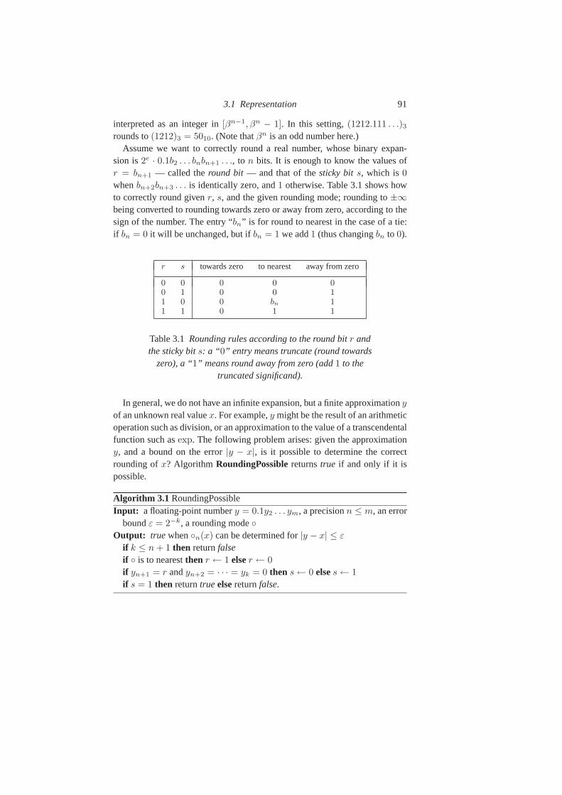
3.1 Representation 91
interpreted as an integer in[βn−1, βn − 1]. In this setting,(1212.111 . . .)3rounds to(1212)3 = 5010. (Note thatβn is an odd number here.)
Assume we want to correctly round a real number, whose binaryexpan-sion is2e · 0.1b2 . . . bnbn+1 . . ., to n bits. It is enough to know the values ofr = bn+1 — called theround bit — and that of thesticky bits, which is0
whenbn+2bn+3 . . . is identically zero, and1 otherwise. Table 3.1 shows howto correctly round givenr, s, and the given rounding mode; rounding to±∞being converted to rounding towards zero or away from zero, according to thesign of the number. The entry “bn” is for round to nearest in the case of a tie:if bn = 0 it will be unchanged, but ifbn = 1 we add1 (thus changingbn to 0).
r s towards zero to nearest away from zero
0 0 0 0 00 1 0 0 11 0 0 bn 11 1 0 1 1
Table 3.1Rounding rules according to the round bitr andthe sticky bits: a “ 0” entry means truncate (round towards
zero), a “1” means round away from zero (add1 to thetruncated significand).
In general, we do not have an infinite expansion, but a finite approximationyof an unknown real valuex. For example,y might be the result of an arithmeticoperation such as division, or an approximation to the valueof a transcendentalfunction such asexp. The following problem arises: given the approximationy, and a bound on the error|y − x|, is it possible to determine the correctrounding ofx? Algorithm RoundingPossiblereturnstrue if and only if it ispossible.
Algorithm 3.1 RoundingPossibleInput: a floating-point numbery = 0.1y2 . . . ym, a precisionn ≤ m, an error
boundε = 2−k, a rounding modeOutput: truewhenn(x) can be determined for|y − x| ≤ ε
if k ≤ n + 1 then returnfalseif is to nearestthen r ← 1 elser ← 0
if yn+1 = r andyn+2 = · · · = yk = 0 then s ← 0 elses ← 1
if s = 1 then returntrueelsereturnfalse.
92 Floating-Point Arithmetic
Proof. Since rounding is monotonic, it is possible to determine(x) exactlywhen(y− 2−k) = (y +2−k), or in other words when the interval[y− 2−k,
y + 2−k] contains no rounding boundary (or only one asy − 2−k or y + 2−k).If k ≤ n + 1, then the interval[−2−k, 2−k] has width at least2−n, thus
contains at least one rounding boundary in its interior, or two rounding bound-aries, and it is not possible to round correctly. In the case of directed round-ing (resp. rounding to nearest), ifs = 0 the approximationy is representable(resp. the middle of two representable numbers) in precision n, and it is clearlynot possible to round correctly; ifs = 1 the interval[y − 2−k, y + 2−k] con-tains at most one rounding boundary, and if so it is one of the bounds, thus itis possible to round correctly.
The Double Rounding ProblemWhen a given real valuex is first rounded to precisionm, then to precisionn < m, we say that a “double rounding” occurs. The “double rounding prob-lem” happens when this latter value differs from the direct rounding ofx tothe smaller precisionn, assuming the same rounding mode is used in all cases,i.e., when:
n(m(x)) 6= n(x).
The double rounding problem does not occur for directed rounding modes.For these rounding modes, the rounding boundaries at the larger precisionmrefine those at the smaller precisionn, thus all real valuesx that round to thesame valuey at precisionm also round to the same value at precisionn, namelyn(y).
Consider the decimal valuex = 3.14251. Rounding to nearest to5 digits, wegety = 3.1425; roundingy to nearest-even to4 digits, we get3.142, whereasdirect rounding ofx would give3.143.
With rounding to nearest mode, the double rounding problem only occurswhen the second rounding involves the even-rule, i.e., the valuey = m(x) isa rounding boundary at precisionn. Otherwisey has distance at least one ulp(in precisionm) from a rounding boundary at precisionn, and since|y − x| isbounded by half an ulp (in precisionm), all possible values forx round to thesame value in precisionn.
Note that the double rounding problem does not occur with allways ofbreaking ties for rounding to nearest (Exercise 3.2).
3.2 Addition, Subtraction, Comparison 93
3.1.10 Strategies
To determine the correct rounding off(x) with n bits of precision, the beststrategy is usually to first compute an approximationy to f(x) with a workingprecision ofm = n+h bits, withh relatively small. Several strategies are pos-sible in Ziv’s algorithm (§3.1.8) when this first approximationy is not accurateenough, or too close to a rounding boundary:
• compute the exact value off(x), and round it to the target precisionn.This is possible for a basic operation, for examplef(x) = x2, or moregenerallyf(x, y) = x + y or x × y. Some elementary functions may yieldan exactly representable output too, for example
√2.25 = 1.5. An “exact
result” test after the first approximation avoids possibly unnecessary furthercomputations;
• repeat the computation with a larger working precisionm′ = n+h′. Assum-ing that the digits off(x) behave “randomly” and that|f ′(x)/f(x)| is nottoo large, usingh′ ≈ lg n is enough to guarantee that rounding is possiblewith probability1 − O(1/n). If rounding is still not possible, because theh′ last digits of the approximation encode0 or 2h′ − 1, one can increase theworking precision and try again. A check for exact results guarantees thatthis process will eventually terminate, provided the algorithm used has theproperty that it gives the exact result if this result is representable and theworking precision is high enough. For example, the square root algorithmshould return the exact result if it is representable (see AlgorithmFPSqrt in§3.5, and also Exercise 3.3).
3.2 Addition, Subtraction, Comparison
Addition and subtraction of floating-point numbers operatefrom the most sig-nificant digits, whereas integer addition and subtraction start from the leastsignificant digits. Thus completely different algorithms are involved. Also, inthe floating-point case, part or all of the inputs might have no impact on theoutput, except in the rounding phase.
In summary, floating-point addition and subtraction are more difficult to im-plement than integer addition/subtraction for two reasons:
• scaling due to the exponents requires shifting the significands before addingor subtracting them. In principle one could perform all operations using onlyinteger operations, but this might require huge integers, for example whenadding1 and2−1000;
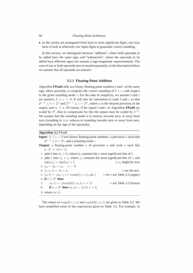
94 Floating-Point Arithmetic
• as the carries are propagated from least to most significant digits, one mayhave to look at arbitrarily low input digits to guarantee correct rounding.
In this section, we distinguish between “addition”, where both operands tobe added have the same sign, and “subtraction”, where the operands to beadded have different signs (we assume a sign-magnitude representation). Thecase of one or both operands zero is treated separately; in the description belowwe assume that all operands are nonzero.
3.2.1 Floating-Point Addition
Algorithm FPadd adds two binary floating-point numbersb andc of the samesign. More precisely, it computes the correct rounding ofb + c, with respectto the given rounding mode. For the sake of simplicity, we assumeb andc
are positive,b ≥ c > 0. It will also be convenient to scaleb and c so that2n−1 ≤ b < 2n and2m−1 ≤ c < 2m, wheren is the desired precision of theoutput, andm ≤ n. Of course, if the inputsb andc to Algorithm FPadd arescaled by2k, then to compensate for this the output must be scaled by2−k.We assume that the rounding mode is to nearest, towards zero,or away fromzero (rounding to±∞ reduces to rounding towards zero or away from zero,depending on the sign of the operands).
Algorithm 3.2 FPaddInput: b ≥ c > 0 two binary floating-point numbers, a precisionn such that
2n−1 ≤ b < 2n, and a rounding modeOutput: a floating-point numbera of precision n and scalee such that
a · 2e = (b + c)
1: split b into bh + bℓ wherebh contains then most significant bits ofb.2: split c into ch + cℓ wherech contains the most significant bits ofc, and
ulp(ch) = ulp(bh) = 1 ⊲ ch might be zero3: ah ← bh + ch, e ← 0
4: (c, r, s) ← bℓ + cℓ ⊲ see the text5: (a, t) ← (ah + c + round(, r, s), etc.) ⊲ for t see Table 3.2 (upper)6: if a ≥ 2n then7: (a, e) ← (round2(, a, t), e + 1) ⊲ see Table 3.2 (lower)8: if a = 2n then (a, e) ← (a/2, e + 1)
9: return(a, e).
The values ofround(, r, s) andround2(, a, t) are given in Table 3.2. Wehave simplified some of the expressions given in Table 3.2. For example, in
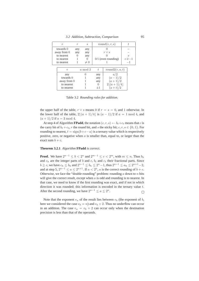
3.2 Addition, Subtraction, Comparison 95
r s round(, r, s) t
towards0 any any 0 –away from0 any any r ∨ s –
to nearest 0 any 0 sto nearest 1 0 0/1 (even rounding) +1/−1to nearest 1 6= 0 1 −1
a mod 2 t round2(, a, t)
any 0 any a/2towards0 1 any (a − 1)/2
away from0 1 any (a + 1)/2to nearest 1 0 2⌊(a + 1)/4⌋to nearest 1 ±1 (a + t)/2
Table 3.2Rounding rules for addition.
the upper half of the table,r ∨ s means0 if r = s = 0, and1 otherwise. Inthe lower half of the table,2⌊(a + 1)/4⌋ is (a − 1)/2 if a = 1 mod 4, and(a + 1)/2 if a = 3 mod 4.
At step 4 of AlgorithmFPadd, the notation(c, r, s) ← bℓ+cℓ means thatc isthe carry bit ofbℓ + cℓ, r the round bit, ands the sticky bit;c, r, s ∈ 0, 1. Forrounding to nearest,t = sign(b+c−a) is a ternary value which is respectivelypositive, zero, or negative whena is smaller than, equal to, or larger than theexact sumb + c.
Theorem 3.2.1 AlgorithmFPadd is correct.
Proof. We have2n−1 ≤ b < 2n and2m−1 ≤ c < 2m, with m ≤ n. Thusbh
andch are the integer parts ofb andc, bℓ andcℓ their fractional parts. Sinceb ≥ c, we havech ≤ bh and2n−1 ≤ bh ≤ 2n−1, thus2n−1 ≤ ah ≤ 2n+1−2,and at step 5,2n−1 ≤ a ≤ 2n+1. If a < 2n, a is the correct rounding ofb + c.Otherwise, we face the “double rounding” problem: roundinga down ton bitswill give the correct result, except whena is odd and rounding is to nearest. Inthat case, we need to know if the first rounding was exact, and if not in whichdirection it was rounded; this information is encoded in theternary valuet.After the second rounding, we have2n−1 ≤ a ≤ 2n.
Note that the exponentea of the result lies betweeneb (the exponent ofb,here we considered the caseeb = n) andeb + 2. Thus no underflow can occurin an addition. The caseea = eb + 2 can occur only when the destinationprecision is less than that of the operands.
96 Floating-Point Arithmetic
3.2.2 Floating-Point Subtraction
Floating-point subtraction (of positive operands) is verysimilar to addition,with the difference thatcancellationcan occur. Consider for example the sub-traction6.77823− 5.98771. The most significant digit of both operands disap-peared in the result0.79052. This cancellation can be dramatic, as in6.7782357934 − 6.7782298731 = 0.0000059203, where six digits were can-celled.
Two approaches are possible, assumingn result digits are wanted, and theexponent difference between the inputs isd:
• subtract then − d most-significant digits of the smaller operand from then
most-significant digits of the larger operand. If the resulthasn − e digitswith e > 0, restart withn+ e digits from the larger operand and(n+ e)−d
from the smaller operand;• alternatively, predict the numbere of cancelled digits in the subtraction, and
directly subtract the(n+e)−d most-significant digits of the smaller operandfrom then + e most-significant digits of the larger one.
Note that in the first approach, we might havee = n if all most-significantdigits cancel, thus the process might need to be repeated several times.
The first step in the second approach is usually calledleading zero detec-tion. Note that the numbere of cancelled digits might depend on the roundingmode. For example,6.778 − 5.7781 with a 3-digit result yields0.999 withrounding toward zero, and1.00 with rounding to nearest. Therefore, in a realimplementation, the definition ofe has to be made precise.
In practice we might considern + g and(n + g)− d digits instead ofn andn − d, where theg “guard digits” would prove useful (i) to decide the finalrounding, and/or (ii) to avoid another loop in casee ≤ g.
Sterbenz’s TheoremSterbenz’s Theorem is an important result concerning floating-point subtrac-tion (of operands of the same sign). It states that the rounding error is zero insome common cases. More precisely:
Theorem 3.2.2 (Sterbenz)If x andy are two floating-point numbers of sameprecisionn, such thaty lies in the interval[x/2, 2x] ∪ [2x, x/2], theny − x isexactly representable in precisionn, if there is no underflow.
Proof. The casex = y = 0 is trivial, so assume thatx 6= 0. Sincey ∈[x/2, 2x] ∪ [2x, x/2], x andy must have the same sign. We assume withoutloss of generality thatx andy are positive, soy ∈ [x/2, 2x].
3.3 Multiplication 97
Assumex ≤ y ≤ 2x (the same reasoning applies forx/2 ≤ y ≤ x, i.e.,y ≤x ≤ 2y, by interchangingx andy). Sincex ≤ y, we haveulp(x) ≤ ulp(y),thus y is an integer multiple ofulp(x). It follows that y − x is an integermultiple of ulp(x). Since0 ≤ y − x ≤ x, y − x is necessarily representablewith the precision ofx.
It is important to note that Sterbenz’s Theorem applies for any radix β; theconstant2 in [x/2, 2x] has nothing to do with the radix.
3.3 Multiplication
Multiplication of floating-point numbers is called ashort product. This reflectsthe fact that, in some cases, the low part of the full product of the signifi-cands has no impact — except perhaps for the rounding — on the final re-sult. Consider the multiplicationx × y, wherex = ℓβe andy = mβf . Then(xy) = (ℓm)βe+f , thus it suffices to consider the case thatx = ℓ andy = m
are integers, and the product is rounded at some weightβg for g ≥ 0. Eitherthe integer productℓ × m is computed exactly, using one of the algorithmsfrom Chapter 1, and then rounded; or the upper part is computed directly usinga “short product algorithm”, with correct rounding. The different cases that canoccur are depicted in Figure 3.1.
An interesting question is: how many consecutive identicalbits can occurafter the round bit? Without loss of generality, we can rephrase this questionas follows. Given two odd integers of at mostn bits, what is the longest run ofidentical bits in their product? (In the case of an even significand, one mightwrite it m = ℓ2e with ℓ odd.) There is noa priori bound except the trivial oneof 2n − 2 for the number of zeros, and2n − 1 for the number of ones. Forexample, with a precision5 bits,27× 19 = (1 000 000 001)2. More generally,such a case corresponds to a factorisation of22n−1 + 1 into two integers ofn bits, for example258 513 × 132 913 = 235 + 1. 2n consecutive ones arenot possible since22n − 1 can not factor into two integers of at mostn bits.Therefore the maximal runs have2n − 1 ones, for example217 × 151 =
(111 111 111 111 111)2 for n = 8. A larger example is849 583 × 647 089 =
239 − 1.The exact product of two floating-point numbersmβe and m′βe′
is(mm′)βe+e′
. Therefore, if no underflow or overflow occurs, the problem re-duces to the multiplication of the significandsm and m′. See AlgorithmFPmultiply .
The product at step 1 ofFPmultiply is ashort product, i.e., a product whose
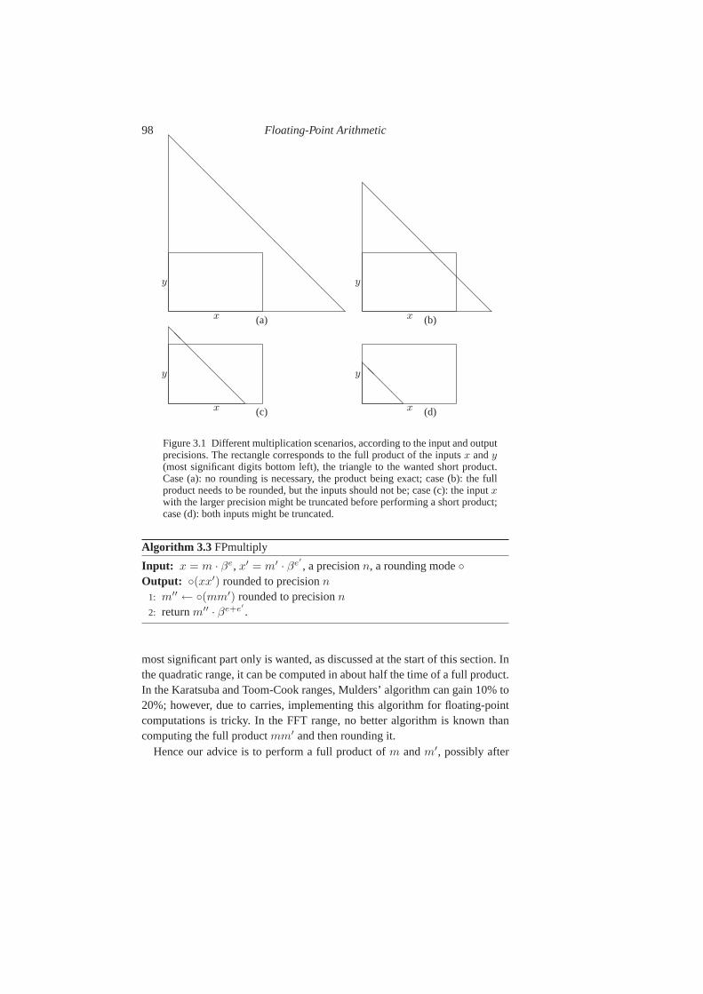
98 Floating-Point Arithmetic
x
y
@@
@@
@@
@@
@@
@@
@@
@
x
y
@@
@@
@@
@@
@@
@
(a) (b)
x
y
@@
@@
@@@
x
y
@@
@@
(c) (d)
Figure 3.1 Different multiplication scenarios, according to the input and outputprecisions. The rectangle corresponds to the full product of the inputsx andy(most significant digits bottom left), the triangle to the wanted short product.Case (a): no rounding is necessary, the product being exact; case (b): the fullproduct needs to be rounded, but the inputs should not be; case (c):the inputxwith the larger precision might be truncated before performing a short product;case (d): both inputs might be truncated.
Algorithm 3.3 FPmultiply
Input: x = m · βe, x′ = m′ · βe′
, a precisionn, a rounding modeOutput: (xx′) rounded to precisionn
1: m′′ ← (mm′) rounded to precisionn2: returnm′′ · βe+e′
.
most significant part only is wanted, as discussed at the start of this section. Inthe quadratic range, it can be computed in about half the timeof a full product.In the Karatsuba and Toom-Cook ranges, Mulders’ algorithm can gain 10% to20%; however, due to carries, implementing this algorithm for floating-pointcomputations is tricky. In the FFT range, no better algorithm is known thancomputing the full productmm′ and then rounding it.
Hence our advice is to perform a full product ofm andm′, possibly after

3.3 Multiplication 99
truncating them ton+ g digits if they have more thann+ g digits. Hereg (thenumber ofguard digits) should be positive (see Exercise 3.4).
It seems wasteful to multiplyn-bit operands, producing a2n-bit product,only to discard the low-ordern bits. Algorithm ShortProduct computes anapproximation to the short product without computing the2n-bit full product.It uses a thresholdn0 ≥ 1, which should be optimized for the given code base.
Error analysis of the short product. Consider twon-word normalised sig-nificandsA andB that we multiply using a short product algorithm, where thenotationFullProduct(A,B) means the full integer productA · B.
Algorithm 3.4 ShortProductInput: integersA,B, andn, with 0 ≤ A,B < βn
Output: an approximation toAB div βn
Require: a thresholdn0
if n ≤ n0 then returnFullProduct(A,B) div βn
choosek ≥ n/2, ℓ ← n − k
C1 ← FullProduct(A div βℓ, B div βℓ) div βk−ℓ
C2 ← ShortProduct(A mod βℓ, B div βk, ℓ)
C3 ← ShortProduct(A div βk, B mod βℓ, ℓ)
returnC1 + C2 + C3.
@
@@
@@
@
@
A
B
C1
C2
C3
C′2
C′3
C4
Figure 3.2 Graphical view of AlgorithmShortProduct:the computed parts areC1, C2, C3, and the neglectedparts areC′
2, C′3, C4 (most significant part bottom left).
Theorem 3.3.1 The valueC ′ returned by AlgorithmShortProduct differs fromthe exact short productC = AB div βn by at most3(n − 1):
C ′ ≤ C ≤ C ′ + 3(n − 1).
100 Floating-Point Arithmetic
Proof. First, sinceA,B are nonnegative, and all roundings are truncations, theinequalityC ′ ≤ C follows.
Let A =∑
i aiβi andB =
∑j bjβ
j , where0 ≤ ai, bj < β. The possibleerrors come from: (i) the neglectedaibj terms, i.e., partsC ′
2, C′3, C4 of Fig-
ure 3.2; (ii) the truncation while computingC1; (iii) the error in the recursivecalls forC2 andC3.
We first prove that the algorithm accumulates all productsaibj with i +
j ≥ n − 1. This corresponds to all terms on and below the diagonal in Fig-ure 3.2. The most significant neglected terms are the bottom-left terms fromC ′
2 andC ′3, respectivelyaℓ−1bk−1 andak−1bℓ−1. Their contribution is at most
2(β−1)2βn−2. The neglected terms from the next diagonal contribute at most4(β − 1)2βn−3, and so on. The total contribution of neglected terms is thusbounded by:
(β − 1)2βn[2β−2 + 4β−3 + 6β−4 + · · · ] < 2βn
(the inequality is strict since the sum is finite).The truncation error inC1 is at mostβn, thus the maximal differenceε(n)
betweenC andC ′ satisfies:
ε(n) < 3 + 2ε(⌊n/2⌋),
which givesε(n) < 3(n − 1), sinceε(1) = 0.
REMARK : if one of the operands was truncated before applying AlgorithmShortProduct, simply add one unit to the upper bound (the truncated part isless than1, thus its product by the other operand is bounded byβn).
The complexityS(n) of Algorithm ShortProduct satifies the recurrenceS(n) = M(k)+2S(n−k). The optimal choice ofk depends on the underlyingmultiplication algorithm. AssumingM(n) ≈ nα for α > 1 andk = γn, weget
S(n) =γα
1 − 2(1 − γ)αM(n),
where the optimal value isγ = 1/2 in the quadratic range,γ ≈ 0.694 inthe Karatsuba range, andγ ≈ 0.775 in the Toom-Cook3-way range, givingrespectivelyS(n) ∼ 0.5M(n), S(n) ∼ 0.808M(n), andS(n) ∼ 0.888M(n).The ratioS(n)/M(n) → 1 as r → ∞ for Toom-Cookr-way. In the FFTrange, AlgorithmShortProduct is not any faster than a full product.
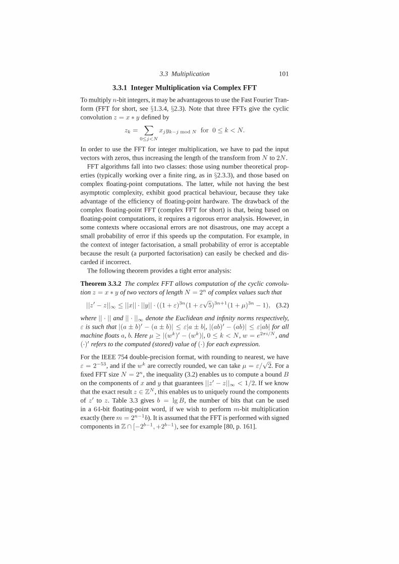
3.3 Multiplication 101
3.3.1 Integer Multiplication via Complex FFT
To multiplyn-bit integers, it may be advantageous to use the Fast FourierTran-form (FFT for short, see§1.3.4,§2.3). Note that three FFTs give the cyclicconvolutionz = x ∗ y defined by
zk =∑
0≤j<N
xjyk−j mod N for 0 ≤ k < N.
In order to use the FFT for integer multiplication, we have topad the inputvectors with zeros, thus increasing the length of the transform fromN to 2N .
FFT algorithms fall into two classes: those using number theoretical prop-erties (typically working over a finite ring, as in§2.3.3), and those based oncomplex floating-point computations. The latter, while nothaving the bestasymptotic complexity, exhibit good practical behaviour,because they takeadvantage of the efficiency of floating-point hardware. The drawback of thecomplex floating-point FFT (complex FFT for short) is that, being based onfloating-point computations, it requires a rigorous error analysis. However, insome contexts where occasional errors are not disastrous, one may accept asmall probability of error if this speeds up the computation. For example, inthe context of integer factorisation, a small probability of error is acceptablebecause the result (a purported factorisation) can easily be checked and dis-carded if incorrect.
The following theorem provides a tight error analysis:
Theorem 3.3.2 The complex FFT allows computation of the cyclic convolu-tion z = x ∗ y of two vectors of lengthN = 2n of complex values such that
||z′ − z||∞ ≤ ||x|| · ||y|| · ((1 + ε)3n(1 + ε√
5)3n+1(1 + µ)3n − 1), (3.2)
where|| · || and || · ||∞ denote the Euclidean and infinity norms respectively,ε is such that|(a ± b)′ − (a ± b)| ≤ ε|a ± b|, |(ab)′ − (ab)| ≤ ε|ab| for allmachine floatsa, b. Hereµ ≥ |(wk)′ − (wk)|, 0 ≤ k < N , w = e2πi/N , and(·)′ refers to the computed (stored) value of(·) for each expression.
For the IEEE 754 double-precision format, with rounding to nearest, we haveε = 2−53, and if thewk are correctly rounded, we can takeµ = ε/
√2. For a
fixed FFT sizeN = 2n, the inequality (3.2) enables us to compute a boundB
on the components ofx andy that guarantees||z′ − z||∞ < 1/2. If we knowthat the exact resultz ∈ ZN , this enables us to uniquely round the componentsof z′ to z. Table 3.3 givesb = lg B, the number of bits that can be usedin a 64-bit floating-point word, if we wish to performm-bit multiplicationexactly (herem = 2n−1b). It is assumed that the FFT is performed with signedcomponents inZ ∩ [−2b−1,+2b−1), see for example [80, p. 161].
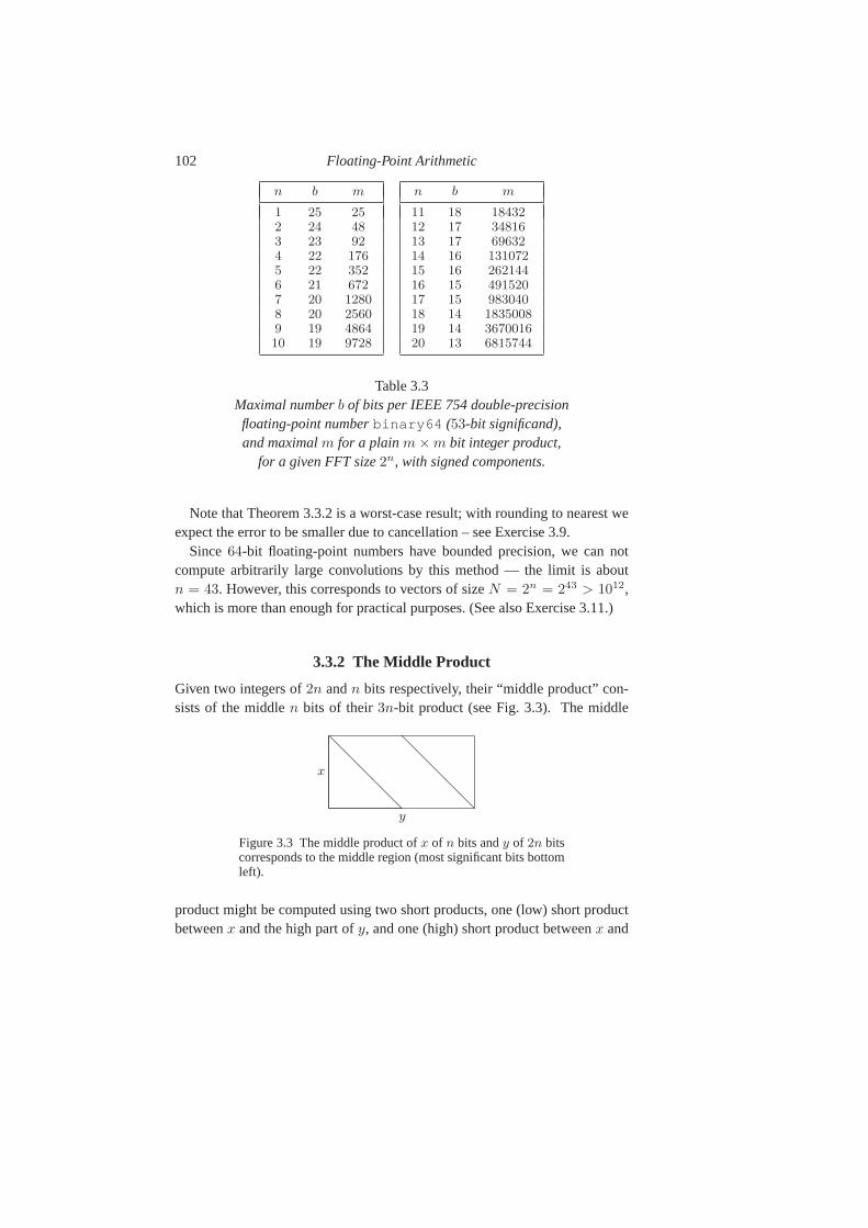
102 Floating-Point Arithmetic
n b m
1 25 252 24 483 23 924 22 1765 22 3526 21 6727 20 12808 20 25609 19 486410 19 9728
n b m
11 18 1843212 17 3481613 17 6963214 16 13107215 16 26214416 15 49152017 15 98304018 14 183500819 14 367001620 13 6815744
Table 3.3Maximal numberb of bits per IEEE 754 double-precisionfloating-point numberbinary64 (53-bit significand),and maximalm for a plainm × m bit integer product,
for a given FFT size2n, with signed components.
Note that Theorem 3.3.2 is a worst-case result; with rounding to nearest weexpect the error to be smaller due to cancellation – see Exercise 3.9.
Since64-bit floating-point numbers have bounded precision, we can notcompute arbitrarily large convolutions by this method — thelimit is aboutn = 43. However, this corresponds to vectors of sizeN = 2n = 243 > 1012,which is more than enough for practical purposes. (See also Exercise 3.11.)
3.3.2 The Middle Product
Given two integers of2n andn bits respectively, their “middle product” con-sists of the middlen bits of their3n-bit product (see Fig. 3.3). The middle
y
x
@@
@@
@
@@
@@
@
Figure 3.3 The middle product ofx of n bits andy of 2n bitscorresponds to the middle region (most significant bits bottomleft).
product might be computed using two short products, one (low) short productbetweenx and the high part ofy, and one (high) short product betweenx and
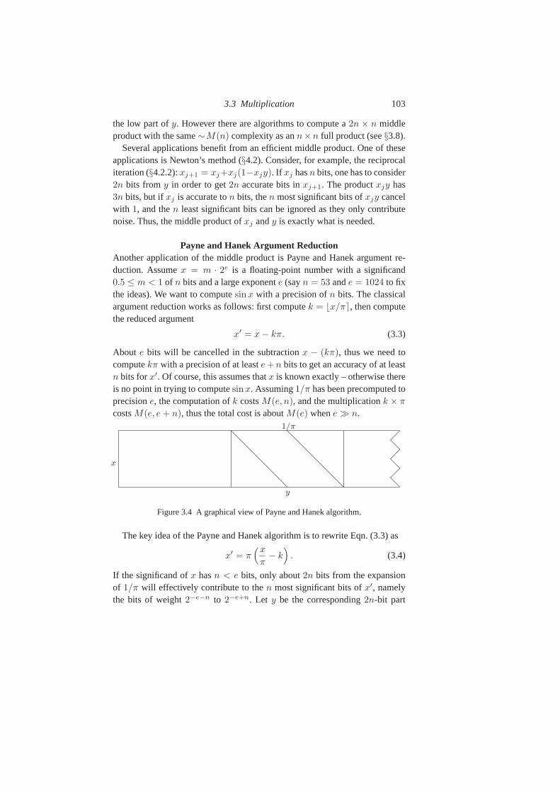
3.3 Multiplication 103
the low part ofy. However there are algorithms to compute a2n × n middleproduct with the same∼M(n) complexity as ann×n full product (see§3.8).
Several applications benefit from an efficient middle product. One of theseapplications is Newton’s method (§4.2). Consider, for example, the reciprocaliteration (§4.2.2):xj+1 = xj+xj(1−xjy). If xj hasn bits, one has to consider2n bits fromy in order to get2n accurate bits inxj+1. The productxjy has3n bits, but ifxj is accurate ton bits, then most significant bits ofxjy cancelwith 1, and then least significant bits can be ignored as they only contributenoise. Thus, the middle product ofxj andy is exactly what is needed.
Payne and Hanek Argument ReductionAnother application of the middle product is Payne and Hanekargument re-duction. Assumex = m · 2e is a floating-point number with a significand0.5 ≤ m < 1 of n bits and a large exponente (sayn = 53 ande = 1024 to fixthe ideas). We want to computesin x with a precision ofn bits. The classicalargument reduction works as follows: first computek = ⌊x/π⌉, then computethe reduced argument
x′ = x − kπ. (3.3)
About e bits will be cancelled in the subtractionx − (kπ), thus we need tocomputekπ with a precision of at leaste + n bits to get an accuracy of at leastn bits forx′. Of course, this assumes thatx is known exactly – otherwise thereis no point in trying to computesin x. Assuming1/π has been precomputed toprecisione, the computation ofk costsM(e, n), and the multiplicationk × π
costsM(e, e + n), thus the total cost is aboutM(e) whene ≫ n.
y
x
1/π
@@
@@
@@
@@
@@
@@
@¡@¡@¡
Figure 3.4 A graphical view of Payne and Hanek algorithm.
The key idea of the Payne and Hanek algorithm is to rewrite Eqn. (3.3) as
x′ = π(x
π− k
). (3.4)
If the significand ofx hasn < e bits, only about2n bits from the expansionof 1/π will effectively contribute to then most significant bits ofx′, namelythe bits of weight2−e−n to 2−e+n. Let y be the corresponding2n-bit part
104 Floating-Point Arithmetic
of 1/π. Payne and Hanek’s algorithm works as follows: first multiply the n-bit significand ofx by y, keep then middle bits, and multiply by ann-bitapproximation ofπ. The total cost is∼(M(2n, n)+M(n)), or even∼2M(n)
if the middle product is performed in timeM(n), thus independent ofe.
3.4 Reciprocal and Division
As for integer operations (§1.4), one should try as far as possible to tradefloating-point divisions for multiplications, since the cost of a floating-pointmultiplication is theoretically smaller than the cost of a division by a constantfactor (usually from2 to 5, depending on the algorithm used). In practice, theratio might not even be constant unless care is taken in implementing division.Some implementations provide division with costΘ(M(n) log n) or Θ(n2).
When several divisions have to be performed with the same divisor, a well-known trick is to first compute the reciprocal of the divisor (§3.4.1); then eachdivision reduces to a multiplications by the reciprocal. A small drawback isthat each division incurs two rounding errors (one for the reciprocal and one formultiplication by the reciprocal) instead of one, so we can no longer guaranteea correctly rounded result. For example, in base ten with sixdigits, 3.0/3.0
might evaluate to0.999 999 = 3.0 × 0.333 333.The cases of a single division, or several divisions with a varying divisor,
are considered in§3.4.2.
3.4.1 Reciprocal
Here we describe algorithms that compute an approximate reciprocal of a pos-itive floating-point numbera, using integer-only operations (see Chapter 1).The integer operations simulate floating-point computations, but all roundingsare made explicit. The numbera is represented by an integerA of n words inradix β: a = β−nA, and we assumeβn/2 ≤ A, thus requiring1/2 ≤ a < 1.(This does not cover all cases forβ ≥ 3, but if βn−1 ≤ A < βn/2, multiplyingA by some appropriate integerk < β will reduce to the caseβn/2 ≤ A, thenit suffices to multiply the reciprocal ofka by k.)
We first perform an error analysis of Newton’s method (§4.2) assuming allcomputations are done with infinite precision, thus neglecting roundoff errors.
Lemma 3.4.1 Let 1/2 ≤ a < 1, ρ = 1/a, x > 0, andx′ = x + x(1 − ax).Then:
0 ≤ ρ − x′ ≤ x2
θ3(ρ − x)2,

3.4 Reciprocal and Division 105
for someθ ∈ [min(x, ρ),max(x, ρ)].
Proof. Newton’s iteration is based on approximating the function by its tan-gent. Letf(t) = a − 1/t, with ρ the root off . The second-order expansion off at t = ρ with explicit remainder is:
f(ρ) = f(x) + (ρ − x)f ′(x) +(ρ − x)2
2f ′′(θ),
for someθ ∈ [min(x, ρ),max(x, ρ)]. Sincef(ρ) = 0, this simplifies to
ρ = x − f(x)
f ′(x)− (ρ − x)2
2
f ′′(θ)
f ′(x). (3.5)
Substitutingf(t) = a− 1/t, f ′(t) = 1/t2 andf ′′(t) = −2/t3, it follows that:
ρ = x + x(1 − ax) +x2
θ3(ρ − x)2,
which proves the claim.
Algorithm ApproximateReciprocal computes an approximate reciprocal.The inputA is assumed to be normalised, i.e.,βn/2 ≤ A < βn. The outputintegerX is an approximation toβ2n/A.
Algorithm 3.5 ApproximateReciprocal
Input: A =∑n−1
i=0 aiβi, with 0 ≤ ai < β andβ/2 ≤ an−1
Output: X = βn +∑n−1
i=0 xiβi with 0 ≤ xi < β
1: if n ≤ 2 then return⌈β2n/A⌉ − 1
2: ℓ ← ⌊(n − 1)/2⌋, h ← n − ℓ
3: Ah ← ∑h−1i=0 aℓ+iβ
i
4: Xh ← ApproximateReciprocal(Ah)
5: T ← AXh
6: while T ≥ βn+h do7: (Xh, T ) ← (Xh − 1, T − A)
8: T ← βn+h − T
9: Tm ← ⌊Tβ−ℓ⌋10: U ← TmXh
11: returnXhβℓ + ⌊Uβℓ−2h⌋.
Lemma 3.4.2 If β is a power of two satisfyingβ ≥ 8, andβn/2 ≤ A < βn,then the outputX of AlgorithmApproximateReciprocal satisfies:
AX < β2n < A(X + 2).
106 Floating-Point Arithmetic
Proof. For n ≤ 2 the algorithm returnsX = ⌊β2n/A⌋, unlessA = βn/2
when it returnsX = 2βn − 1. In both cases we haveAX < β2n ≤ A(X +1),thus the lemma holds forn ≤ 2.
Now considern ≥ 3. We haveℓ = ⌊(n − 1)/2⌋ and h = n − ℓ, thusn = h + ℓ andh > ℓ. The algorithm first computes an approximate reciprocalof the upperh words ofA, and then updates it ton words using Newton’siteration.
After the recursive call at line 4, we have by induction
AhXh < β2h < Ah(Xh + 2). (3.6)
After the productT ← AXh and the while-loop at steps 6–7, we still haveT = AXh, whereT andXh may have new values, and in additionT < βn+h.We also haveβn+h < T + 2A; we prove this by distinguishing two cases.Either we entered the while-loop, then since the value ofT decreased byA ateach loop, the previous valueT + A was necessarily≥ βn+h. If we did notenter the while-loop, the value ofT is still AXh. Multiplying Eqn. (3.6) byβℓ
gives:βn+h < Ahβℓ(Xh + 2) ≤ A(Xh + 2) = T + 2A. Thus we have:
T < βn+h < T + 2A.
It follows thatT > βn+h−2A > βn+h−2βn. As a consequence, the value ofβn+h−T computed at step 8 can not exceed2βn−1. The last lines compute theproductTmXh, whereTm is the upper part ofT , and put itsℓ most significantwords in the low partXℓ of the resultX.
Now let us perform the error analysis. Compared to Lemma 3.4.1, x standsfor Xhβ−h, a stands forAβ−n, andx′ stands forXβ−n. The while-loop en-sures that we start from an approximationx < 1/a, i.e.,AXh < βn+h. ThenLemma 3.4.1 guarantees thatx ≤ x′ ≤ 1/a if x′ is computed with infiniteprecision. Here we havex ≤ x′, sinceX = Xhβh + Xℓ, whereXℓ ≥ 0. Theonly differences compared to infinite precision are:
• the lowℓ words from1 − ax — hereT at line 8 — are neglected, and onlyits upper part(1 − ax)h — hereTm — is considered;
• the low2h − ℓ words fromx(1 − ax)h are neglected.
Those two approximations make the computed value ofx′ ≤ the value whichwould be computed with infinite precision. Thus, for the computed valuex′,we have:
x ≤ x′ ≤ 1/a.
From Lemma 3.4.1, the mathematical error is bounded byx2θ−3(ρ−x)2 <
4β−2h, sincex2 ≤ θ3 and|ρ−x| < 2β−h. The truncation from1−ax, which
3.4 Reciprocal and Division 107
is multiplied byx < 2, produces an error< 2β−2h. Finally, the truncation ofx(1 − ax)h produces an error< β−n. The final result is thus:
x′ ≤ ρ < x′ + 6β−2h + β−n.
Assuming6β−2h ≤ β−n, which holds as soon asβ ≥ 6 since2h > n, thissimplifies to:
x′ ≤ ρ < x′ + 2β−n,
which gives withx′ = Xβ−n andρ = βn/A:
X ≤ β2n
A< X + 2.
Sinceβ is assumed to be a power of two, equality can hold only whenA isitself a power of two, i.e.,A = βn/2. In this case there is only one valueof Xh that is possible for the recursive call, namelyXh = 2βh − 1. In thiscaseT = βn+h − βn/2 before the while-loop, which is not entered. Thenβn+h−T = βn/2, which multiplied byXh gives (again)βn+h−βn/2, whoseh most significant words areβ − 1. ThusXℓ = βℓ − 1, andX = 2βn − 1.
REMARK . Lemma 3.4.2 might be extended to the caseβn−1 ≤ A < βn or toa radixβ which is not a power of two. However, we prefer to state a restrictedresult with simple bounds.
COMPLEXITY ANALYSIS. Let I(n) be the cost to invert ann-word numberusing AlgorithmApproximateReciprocal. If we neglect the linear costs, wehaveI(n) ≈ I(n/2) + M(n, n/2) + M(n/2), whereM(n, n/2) is the costof an n × (n/2) product — the productAXh at step 5 — andM(n/2) thecost of an(n/2) × (n/2) product — the productTmXh at step 10. If then × (n/2) product is performed via two(n/2) × (n/2) products, we haveI(n) ≈ I(n/2)+3M(n/2), which yieldsI(n) ∼ M(n) in the quadratic range,∼ 1.5M(n) in the Karatsuba range,∼ 1.704M(n) in the Toom-Cook3-wayrange, and∼3M(n) in the FFT range. In the FFT range, ann× (n/2) productmight be directly computed by three FFTs of length3n/2 words, amountingto ∼ M(3n/4); in this case the complexity decreases to∼ 2.5M(n) (see thecomments at the end of§2.3.3, page 58).
THE WRAP-AROUND TRICK. We now describe a slight modification of Al-gorithm ApproximateReciprocal which yields a complexity2M(n). In theproductAXh at step 5, Eqn. (3.6) tells us that the result approachesβn+h, ormore precisely:
βn+h − 2βn < AXh < βn+h + 2βn. (3.7)
108 Floating-Point Arithmetic
Assume we use an FFT-based algorithm such as the Schonhage-Strassen al-gorithm that computes products moduloβm +1, for some integerm ∈ (n, n+
h). Let AXh = Uβm + V with 0 ≤ V < βm. It follows from Eqn. (3.7) thatU = βn+h−m or U = βn+h−m−1. LetT = AXh mod (βm+1) be the valuecomputed by the algorithm. We haveT = V −U or T = V −U + (βm + 1).It follows thatAXh = T + U(βm + 1) or AXh = T + (U − 1)(βm + 1).Taking into account the two possible values ofU , we have
AXh = T + (βn+h−m − ε)(βm + 1),
whereε ∈ 0, 1, 2. Sinceβ ≥ 6, βm > 4βn, thus only one value ofε yieldsa value ofAXh in the interval(βn+h − 2βn, βn+h + 2βn).
Thus, we can replace step 5 in AlgorithmApproximateReciprocal by thefollowing code:
ComputeT = AXh mod (βm + 1) using FFTs with lengthm > nT ← T + βn+h + βn+h−m ⊲ the caseε = 0while T ≥ βn+h + 2βn do
T ← T − (βm + 1)
Assuming that one can takem close ton, the cost of the productAXh isonly about that of three FFTs of lengthn, that is∼M(n/2).
3.4.2 Division
In this section we consider the case where the divisor changes between succes-sive operations, so no precomputation involving the divisor can be performed.We first show that the number of consecutive zeros in the result is bounded bythe divisor length, then we consider the division algorithmand its complexity.Lemma 3.4.3 analyses the case where the division operands are truncated, be-cause they have a larger precision than desired in the result. Finally we discuss“short division” and the error analysis of Barrett’s algorithm.
A floating-point division reduces to an integer division as follows. Assumedividenda = ℓ · βe and divisord = m · βf , whereℓ,m are integers. Thena/d = (ℓ/m)βe−f . If k bits of the quotient are needed, we first determinea scaling factorg such thatβk−1 ≤ |ℓβg/m| < βk, and we divideℓβg —truncated if needed — bym. The following theorem gives a bound on thenumber of consecutive zeros after the integer part of the quotient of ⌊ℓβg⌋ bym.
Theorem 3.4.1 Assume we divide anm-digit positive integer by ann-digitpositive integer in radixβ, with m ≥ n. Then the quotient is either exact, or
3.4 Reciprocal and Division 109
its radixβ expansion admits at mostn − 1 consecutive zeros or ones after thedigit of weightβ0.
Proof. We first consider consecutive zeros. If the expansion of the quotientqadmitsn or more consecutive zeros after the binary point, we can write q =
q1+β−nq0, whereq1 is an integer and0 ≤ q0 < 1. If q0 = 0, then the quotientis exact. Otherwise, ifa is the dividend andd is the divisor, one should havea = q1d+β−nq0d. However,a andq1d are integers, and0 < β−nq0d < 1, soβ−nq0d can not be an integer, so we have a contradiction.
For consecutive ones, the proof is similar: writeq = q1 − β−nq0, with0 ≤ q0 ≤ 1. Sinced < βn, we still have0 ≤ β−nq0d < 1.
Algorithm DivideNewton performs the division of twon-digit floating-point numbers. The key idea is to approximate the inverse of the divisor to halfprecision only, at the expense of additional steps. At step 4, MiddleProduct(q0, d) denotes the middle product ofq0 andd, i.e., then/2 middle digits ofthat product. At step 2,r is an approximation to1/d1, and thus to1/d, withprecisionn/2 digits. Therefore at step 3,q0 approximatesc/d to aboutn/2
digits, and the uppern/2 digits of q0d at step 4 agree with those ofc. Thevaluee computed at step 4 thus equalsq0d− c to precisionn/2. It follows thatre ≈ e/d agrees withq0 − c/d to precisionn/2; hence the correction term(which is really a Newton correction) added in the last step.
Algorithm 3.6 DivideNewtonInput: n-digit floating-point numbersc andd, with n even,d normalisedOutput: an approximation ofc/d
1: write d = d1βn/2 + d0 with 0 ≤ d1, d0 < βn/2
2: r ← ApproximateReciprocal(d1, n/2)
3: q0 ← cr truncated ton/2 digits4: e ← MiddleProduct(q0, d)
5: q ← q0 − re.
In the FFT range, the cost of AlgorithmDivideNewton is∼2.5M(n): step 2costs∼ 2M(n/2) ∼ M(n) with the wrap-around trick, and steps 3–5 eachcost∼M(n/2) — using a fast middle product algorithm for step 4. By way ofcomparison, if we computed a full precision inverse as in Barrett’s algorithm(see below), the cost would be∼3.5M(n). (See§3.8 for improved asymptoticbounds on division.)
In the Karatsuba range, AlgorithmDivideNewton costs∼1.5M(n), and isuseful provided the middle product of step 4 is performed with cost∼M(n/2).
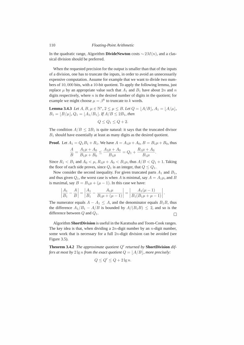
110 Floating-Point Arithmetic
In the quadratic range, AlgorithmDivideNewton costs∼ 2M(n), and a clas-sical division should be preferred.
When the requested precision for the output is smaller than that of the inputsof a division, one has to truncate the inputs, in order to avoid an unnecessarilyexpensive computation. Assume for example that we want to divide two num-bers of10, 000 bits, with a10-bit quotient. To apply the following lemma, justreplaceµ by an appropriate value such thatA1 andB1 have about2n andn
digits respectively, wheren is the desired number of digits in the quotient; forexample we might chooseµ = βk to truncate tok words.
Lemma 3.4.3 LetA,B, µ ∈ N∗, 2 ≤ µ ≤ B. LetQ = ⌊A/B⌋, A1 = ⌊A/µ⌋,B1 = ⌊B/µ⌋, Q1 = ⌊A1/B1⌋. If A/B ≤ 2B1, then
Q ≤ Q1 ≤ Q + 2.
The conditionA/B ≤ 2B1 is quite natural: it says that the truncated divisorB1 should have essentially at least as many digits as the desired quotient.
Proof. Let A1 = Q1B1 + R1. We haveA = A1µ + A0, B = B1µ + B0, thus
A
B=
A1µ + A0
B1µ + B0≤ A1µ + A0
B1µ= Q1 +
R1µ + A0
B1µ.
SinceR1 < B1 andA0 < µ, R1µ + A0 < B1µ, thusA/B < Q1 + 1. Takingthe floor of each side proves, sinceQ1 is an integer, thatQ ≤ Q1.
Now consider the second inequality. For given truncated parts A1 andB1,and thus givenQ1, the worst case is whenA is minimal, sayA = A1µ, andB
is maximal, sayB = B1µ + (µ − 1). In this case we have:∣∣∣∣A1
B1− A
B
∣∣∣∣ =
∣∣∣∣A1
B1− A1µ
B1µ + (µ − 1)
∣∣∣∣ =
∣∣∣∣A1(µ − 1)
B1(B1µ + µ − 1)
∣∣∣∣ .
The numerator equalsA − A1 ≤ A, and the denominator equalsB1B, thusthe differenceA1/B1 − A/B is bounded byA/(B1B) ≤ 2, and so is thedifference betweenQ andQ1.
Algorithm ShortDivision is useful in the Karatsuba and Toom-Cook ranges.The key idea is that, when dividing a2n-digit number by ann-digit number,some work that is necessary for a full2n-digit division can be avoided (seeFigure 3.5).
Theorem 3.4.2 The approximate quotientQ′ returned byShortDivision dif-fers at most by2 lg n from the exact quotientQ = ⌊A/B⌋, more precisely:
Q ≤ Q′ ≤ Q + 2 lg n.
3.4 Reciprocal and Division 111
Algorithm 3.7 ShortDivision
Input: 0 ≤ A < β2n, βn/2 ≤ B < βn
Output: an approximation ofA/B
Require: a thresholdn0
1: if n ≤ n0 then return⌊A/B⌋2: choosek ≥ n/2, ℓ ← n − k
3: (A1, A0) ← (A div β2ℓ, A mod β2ℓ)
4: (B1, B0) ← (B div βℓ, B mod βℓ)
5: (Q1, R1) ← DivRem(A1, B1)
6: A′ ← R1β2ℓ + A0 − Q1B0β
ℓ
7: Q0 ← ShortDivision(A′ div βk, B div βk)
8: returnQ1βℓ + Q0.
Proof. If n ≤ n0, Q = Q′ so the statement holds. Assumen > n0. WehaveA = A1β
2ℓ + A0 andB = B1βℓ + B0, thus sinceA1 = Q1B1 + R1,
A = (Q1B1 + R1)β2ℓ + A0 = Q1Bβℓ + A′, with A′ < βn+ℓ. Let A′ =
A′1β
k+A′0, andB = B′
1βk+B′
0, with 0 ≤ A′0, B
′0 < βk, andA′
1 < β2ℓ. FromLemma 3.4.3, the exact quotient ofA′ div βk by B div βk is greater or equalto that ofA′ byB, thus by inductionQ0 ≥ A′/B. SinceA/B = Q1β
ℓ+A′/B,this proves thatQ′ ≥ Q.
Now by inductionQ0 ≤ A′1/B′
1 + 2 lg ℓ, andA′1/B′
1 ≤ A′/B + 2 (fromLemma 3.4.3 again, whose hypothesisA′/B ≤ 2B′
1 is satisfied, sinceA′ <
B1β2ℓ, thusA′/B ≤ βℓ ≤ 2B′
1), soQ0 ≤ A′/B + 2 lg n, andQ′ ≤ A/B +
2 lg n.
As shown at the lower half of Figure 3.5, we can use a short product to com-puteQ1B0 at step 6. Indeed, we need only the upperℓ words ofA′, thus onlythe upperℓ words ofQ1B0. The complexity of AlgorithmShortDivision satis-fiesD∗(n) = D(k)+M∗(n−k)+D∗(n−k) with k ≥ n/2, whereD(n) de-notes the cost of a division with remainder, andM∗(n) the cost of a short prod-uct. In the Karatsuba range we haveD(n) ∼ 2M(n), M∗(n) ∼ 0.808M(n),and the best possible value ofk is k ≈ 0.542n, with corresponding costD∗(n) ∼ 1.397M(n). In the Toom-Cook3-way range,k ≈ 0.548n is op-timal, and givesD∗(n) ∼ 1.988M(n).
Barrett’s floating-point division algorithmHere we consider floating-point division using Barrett’s algorithm and providea rigorous error bound (see§2.4.1 for an exact integer version). The algorithm
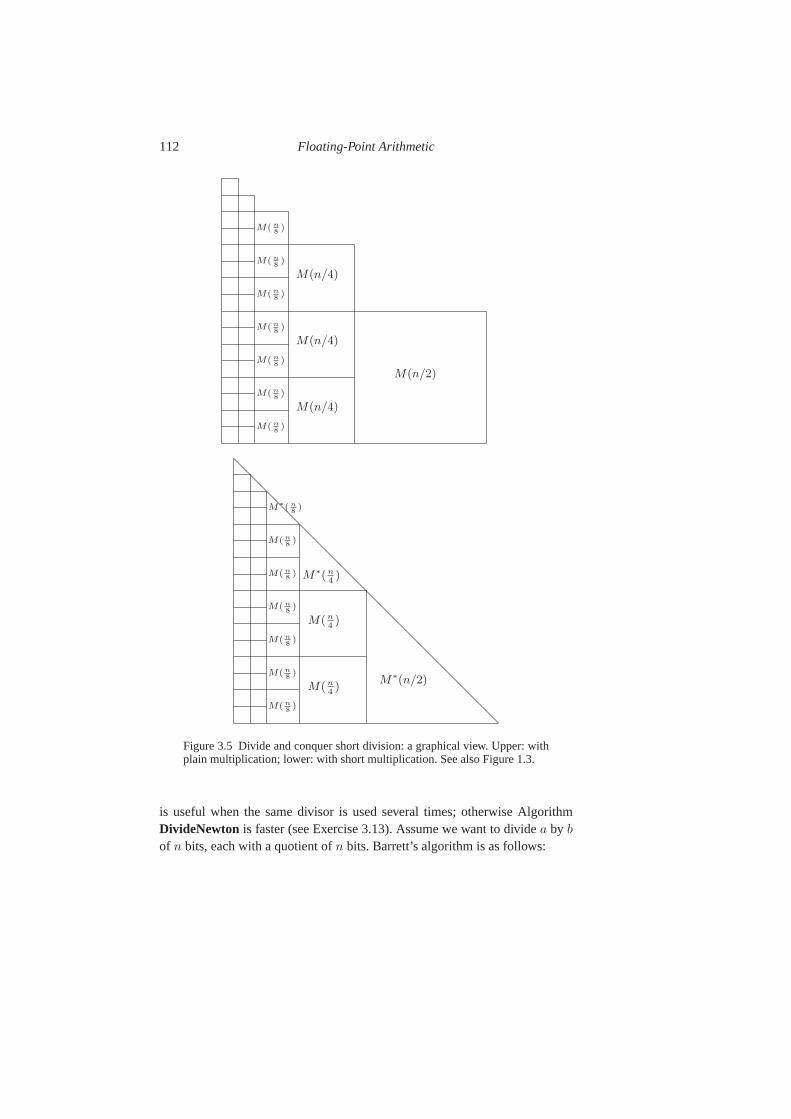
112 Floating-Point Arithmetic
M(n/2)
M(n/4)
M(n/4)
M(n/4)
M( n8)
M( n8)
M( n8)
M( n8)
M( n8)
M( n8)
M( n8)
@@
@@
@@
@@
@@
@@
@@
@@
@@
@@
M∗(n/2)M(n
4)
M(n4)
M∗(n4)
M( n8)
M( n8)
M( n8)
M( n8)
M( n8)
M( n8)
M∗( n8)
Figure 3.5 Divide and conquer short division: a graphical view. Upper: withplain multiplication; lower: with short multiplication. See also Figure 1.3.
is useful when the same divisor is used several times; otherwise AlgorithmDivideNewton is faster (see Exercise 3.13). Assume we want to dividea by b
of n bits, each with a quotient ofn bits. Barrett’s algorithm is as follows:
3.5 Square Root 113
1. Compute the reciprocalr of b to n bits [rounding to nearest]2. q ← n(a × r) [rounding to nearest]
The cost of the algorithm in the FFT range is∼3M(n): ∼2M(n) to computethe reciprocal with the wrap-around trick, andM(n) for the producta × r.
Lemma 3.4.4 At step 2 of Barrett’s algorithm, we have|a − bq| ≤ 3|b|/2.
Proof. By scalinga and b, we can assume thatb and q are integers, that2n−1 ≤ b, q < 2n, thusa < 22n. We haver = 1/b+ε with |ε| ≤ ulp(2−n/2) =
2−2n. Also q = ar + ε′ with |ε′| ≤ ulp(q)/2 = 1/2 sinceq hasn bits. Thusq = a(1/b + ε) + ε′ = a/b + aε + ε′, and|bq − a| = |b||aε + ε′| ≤ 3|b|/2.
As a consequence,q differs by at most one unit in last place from then-bitquotient ofa andb, rounded to nearest.
Lemma 3.4.4 can be applied as follows: to perform several divisions with aprecision ofn bits with the same divisor, precompute a reciprocal withn + g
bits, and use the above algorithm with a working precision ofn + g bits. If thelastg bits of q are neither000 . . . 00x nor111 . . . 11x (wherex stands for0 or1), then roundingq down ton bits will yield n(a/b) for a directed roundingmode.
Which Algorithm to Use?In this section, we described three algorithms to computex/y: Divide-Newtonuses Newton’s method for1/y and incorporates the dividendx at the last itera-tion, ShortDivision is a recursive algorithm using division with remainder andshort products, and Barrett’s algorithm assumes we have precomputed an ap-proximation to1/y. When the same divisory is used several times, clearly Bar-rett’s algorithm is better, since each division costs only ashort product. Oth-erwiseShortDivision is theoretically faster thanDivideNewton in the school-book and Karatsuba ranges, and takingk = n/2 as parameter inShortDivisionis close to optimal. In the FFT range,DivideNewtonshould be preferred.
3.5 Square Root
Algorithm FPSqrt computes a floating-point square root, using as subroutineAlgorithm SqrtRem (§1.5.1 to determine an integer square root (with remain-der). It assumes an integer significandm, and a directed rounding mode (seeExercise 3.14 for rounding to nearest).
Theorem 3.5.1 Algorithm FPSqrt returns the correctly rounded square rootof x.
114 Floating-Point Arithmetic
Algorithm 3.8 FPSqrtInput: x = m · 2e, a target precisionn, a directed rounding modeOutput: y = n(
√x)
if e is oddthen (m′, f) ← (2m, e − 1) else(m′, f) ← (m, e)
definem′ := m122k + m0, m1 integer of2n or 2n − 1 bits,0 ≤ m0 < 22k
(s, r) ← SqrtRem(m1)
if ( is round towards zero or down) or(r = m0 = 0)
then returns · 2k+f/2 elsereturn(s + 1) · 2k+f/2.
Proof. Sincem1 has2n or 2n − 1 bits, s has exactlyn bits, and we havex ≥ s222k+f , thus
√x ≥ s2k+f/2. On the other hand,SqrtRem ensures that
r ≤ 2s, thusx2−f = (s2 + r)22k + m0 < (s2 + r + 1)22k ≤ (s + 1)222k.Sincey := s · 2k+f/2 andy+ = (s + 1) · 2k+f/2 are two consecutiven-bitfloating-point numbers, this concludes the proof.
NOTE: in the cases = 2n − 1, s + 1 = 2n is still representable inn bits.
A different method is to use an initial approximation to the reciprocal squarerootx−1/2 (§3.5.1), see Exercise 3.15. Faster algorithms are mentionedin §3.8.
3.5.1 Reciprocal Square Root
In this section we describe an algorithm to compute the reciprocal square roota−1/2 of a floating-point numbera, with a rigorous error bound.
Lemma 3.5.1 Leta, x > 0, ρ = a−1/2, andx′ = x + (x/2)(1 − ax2). Then
0 ≤ ρ − x′ ≤ 3x3
2θ4(ρ − x)2,
for someθ ∈ [min(x, ρ),max(x, ρ)].
Proof. The proof is very similar to that of Lemma 3.4.1. Here we usef(t) =
a − 1/t2, with ρ the root off . Eqn. (3.5) translates to:
ρ = x +x
2(1 − ax2) +
3x3
2θ4(ρ − x)2,
which proves the Lemma.
Lemma 3.5.2 Provided thatβ ≥ 38, if X is the value returned by AlgorithmApproximateRecSquareRoot, a = Aβ−n, x = Xβ−n, then1/2 ≤ x < 1
and
|x − a−1/2| ≤ 2β−n.
3.5 Square Root 115
Algorithm 3.9 ApproximateRecSquareRootInput: integerA with βn ≤ A < 4βn, β ≥ 38
Output: integerX, βn/2 ≤ X < βn satisfying Lemma 3.5.21: if n ≤ 2 then returnmin(βn − 1, ⌊βn/
√Aβ−n⌋)
2: ℓ ← ⌊(n − 1)/2⌋, h ← n − ℓ
3: Ah ← ⌊Aβ−ℓ⌋4: Xh ← ApproximateRecSquareRoot(Ah)
5: T ← AX2h
6: Th ← ⌊Tβ−n⌋7: Tℓ ← β2h − Th
8: U ← TℓXh
9: returnmin(βn − 1,Xhβℓ + ⌊Uβℓ−2h/2⌉).
Proof. We have1 ≤ a < 4. SinceX is bounded byβn − 1 at lines 1 and 9,we havex, xh < 1, with xh = Xhβ−h. We prove the statement by inductiononn. It is true forn ≤ 2. Now assume the valueXh at step 4 satisfies:
|xh − a−1/2h | ≤ β−h,
whereah = Ahβ−h. We have three sources of error, that we will bound sepa-rately:
1. the rounding errors in steps 6 and 9;
2. the mathematical error given by Lemma 3.5.1, which would occur even ifall computations were exact;
3. the error coming from the fact we useAh instead ofA in the recursive callat step 4.
At step 5 we have exactly:
t := Tβ−n−2h = ax2h,
which gives|th − ax2h| < β−2h with th := Thβ−2h, and in turn|tℓ − (1 −
ax2h)| < β−2h with tℓ := Tℓβ
−2h. At step 8, it follows|u − xh(1 − ax2h)| <
β−2h, whereu = Uβ−3h. Thus, finally|x− [xh+xh(1−ax2h)/2]| < (β−2h+
β−n)/2, after taking into account the rounding error in the last step.Now we apply Lemma 3.5.1 tox → xh, x′ → x, to bound the mathematical
error, assuming no rounding error occurs:
0 ≤ a−1/2 − x ≤ 3x3h
2θ4(a−1/2 − xh)2,
116 Floating-Point Arithmetic
which gives1 |a−1/2 − x| ≤ 3.04(a−1/2 − xh)2. Now |a−1/2 − a−1/2h | ≤
|a − ah|ν−3/2/2 for ν ∈ [min(ah, a),max(ah, a)], thus|a−1/2 − a−1/2h | ≤
β−h/2.Together with the induction hypothesis|xh − a
−1/2h | ≤ 2β−h, it follows that
|a−1/2 − xh| ≤ 2.5β−h. Thus|a−1/2 − x| ≤ 19β−2h.The total error is thus bounded by:
|a−1/2 − x| ≤ 3
2β−n + 19β−2h.
Since2h ≥ n + 1, we see that19β−2h ≤ β−n/2 for β ≥ 38, and the lemmafollows.
NOTE: if AhX2h ≤ β3h at step 4 of AlgorithmApproximateRecSquareRoot,
we could haveAX2h > βn+2h at step 5, which might causeTℓ to be negative.
Let R(n) be the cost ofApproximateRecSquareRootfor ann-digit input.We haveh, ℓ ≈ n/2, thus the recursive call costsR(n/2), step 5 costsM(n/2)
to computeX2h, andM(n) for the productAX2
h (orM(3n/4) in the FFT rangeusing the wrap-around trick described in§3.4.1, since we know the uppern/2
digits of the product give1), and againM(n/2) for step 8. We getR(n) =
R(n/2) + 2M(n) (or R(n/2) + 7M(n)/4 in the FFT range), which yieldsR(n) ∼ 4M(n) (or R(n) ∼ 3.5M(n) in the FFT range).
This algorithm is not optimal in the FFT range, especially when using anFFT algorithm with cheap point-wise products (such as the complex FFT, see§3.3.1). Indeed, AlgorithmApproximateRecSquareRootuses the followingform of Newton’s iteration:
x′ = x +x
2(1 − ax2).
It might be better to write:
x′ = x +1
2(x − ax3).
Here, the productx3 might be computed with asingleFFT transform of length3n/2, replacing the point-wise productsx2
i by x3i , with a total cost∼0.75M(n).
Moreover, the same idea can be used for the full productax3 of 5n/2 bits,whose uppern/2 bits match those ofx. Thus, using the wrap-around trick,
1 Sinceθ ∈ [xh, a−1/2] and|xh − a−1/2| ≤ 2.5β−h, we haveθ ≥ xh − 2.5β−h, thusxh/θ ≤ 1 + 2.5β−h/θ ≤ 1 + 5β−h (rememberθ ∈ [xh, a−1/2]), and it follows thatθ ≥ 1/2. Forβ ≥ 38, sinceh ≥ 2, we have1 + 5β−h ≤ 1.0035, thus1.5x3
h/θ4 ≤ (1.5/θ)(1.0035)3 ≤ 3.04.
3.6 Conversion 117
a transform of length2n is enough, with a cost of∼ M(n) for the last iter-ation, and a total cost of∼ 2M(n) for the reciprocal square root. With thisimprovement, the algorithm of Exercise 3.15 costs only∼2.25M(n).
3.6 Conversion
Since most software tools work in radix2 or 2k, and humans usually enter orread floating-point numbers in radix10 or 10k, conversions are needed fromone radix to the other one. Most applications perform very few conversions,in comparison to other arithmetic operations, thus the efficiency of the conver-sions is rarely critical.2 The main issue here is therefore more correctness thanefficiency. Correctness of floating-point conversions is not an easy task, as canbe seen from the history of bugs in Microsoft Excel.3
The algorithms described in this section use as subroutinesthe integer-conversion algorithms from Chapter 1. As a consequence, their efficiency de-pends on the efficiency of the integer-conversion algorithms.
3.6.1 Floating-Point Output
In this section we follow the convention of using lower-caseletters for param-eters related to the internal radixb, and upper-case for parameters related tothe external radixB. Consider the problem of printing a floating-point num-ber, represented internally in radixb (sayb = 2) in an external radixB (sayB = 10). We distinguish here two kinds of floating-point output:
• fixed-format output, where the output precision is given by the user, andwe want the output value to be correctly rounded according tothe givenrounding mode. This is the usual method when values are to be used byhumans, for example to fill a table of results. The input and output precisionsmay be very different: for example one may want to print1000 digits of2/3,which uses only one digit internally in radix3. Conversely, one may want toprint only a few digits of a number accurate to1000 bits.
• free-format output, where we want the output value, when read with correctrounding (usually to nearest), to giveexactlythe initial number. Here theminimal number of printed digits may depend on the input number. This
2 An important exception is the computation of billions of digits of constants likeπ, log 2,where a quadratic conversion routine would be far too slow.
3 In Excel 2007, the product850 × 77.1 prints as100, 000 instead of65, 535; this is really anoutput bug, since if one multiplies “100, 000” by 2, one gets131, 070. An input bug occurredin Excel 3.0 to 7.0, where the input1.40737488355328 gave0.64.
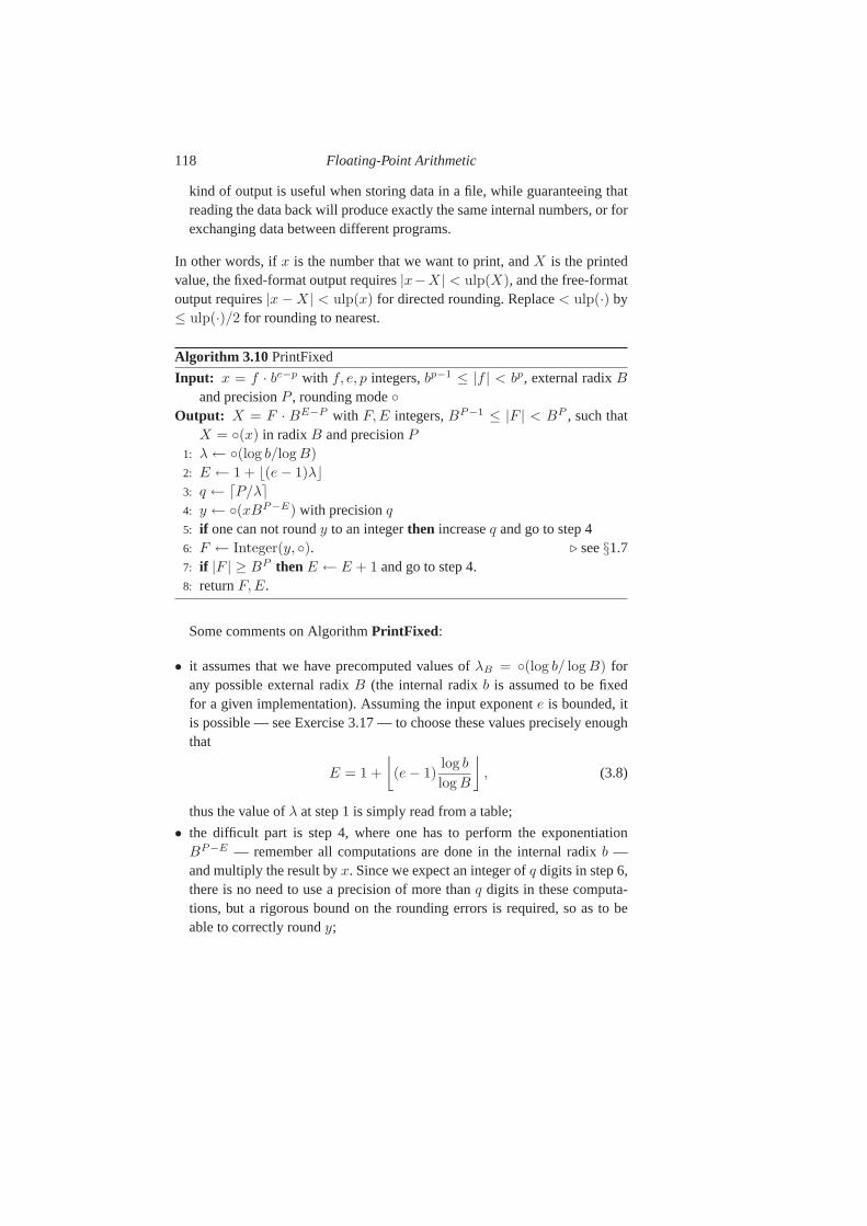
118 Floating-Point Arithmetic
kind of output is useful when storing data in a file, while guaranteeing thatreading the data back will produce exactly the same internalnumbers, or forexchanging data between different programs.
In other words, ifx is the number that we want to print, andX is the printedvalue, the fixed-format output requires|x−X| < ulp(X), and the free-formatoutput requires|x − X| < ulp(x) for directed rounding. Replace< ulp(·) by≤ ulp(·)/2 for rounding to nearest.
Algorithm 3.10 PrintFixed
Input: x = f · be−p with f, e, p integers,bp−1 ≤ |f | < bp, external radixBand precisionP , rounding mode
Output: X = F · BE−P with F,E integers,BP−1 ≤ |F | < BP , such thatX = (x) in radixB and precisionP
1: λ ← (log b/log B)
2: E ← 1 + ⌊(e − 1)λ⌋3: q ← ⌈P/λ⌉4: y ← (xBP−E) with precisionq5: if one can not roundy to an integerthen increaseq and go to step 46: F ← Integer(y, ). ⊲ see§1.77: if |F | ≥ BP then E ← E + 1 and go to step 4.8: returnF,E.
Some comments on AlgorithmPrintFixed :
• it assumes that we have precomputed values ofλB = (log b/ log B) forany possible external radixB (the internal radixb is assumed to be fixedfor a given implementation). Assuming the input exponente is bounded, itis possible — see Exercise 3.17 — to choose these values precisely enoughthat
E = 1 +
⌊(e − 1)
log b
log B
⌋, (3.8)
thus the value ofλ at step 1 is simply read from a table;
• the difficult part is step 4, where one has to perform the exponentiationBP−E — remember all computations are done in the internal radixb —and multiply the result byx. Since we expect an integer ofq digits in step 6,there is no need to use a precision of more thanq digits in these computa-tions, but a rigorous bound on the rounding errors is required, so as to beable to correctly roundy;
3.6 Conversion 119
• in step 5, “one can roundy to an integer” means that the interval contain-ing all possible values ofxBP−E — including the rounding errors whileapproachingxBP−E , and the error while rounding to precisionq — con-tains no rounding boundary (if is a directed rounding, it should contain nointeger; if is rounding to nearest, it should contain no half-integer).
Theorem 3.6.1 AlgorithmPrintFixed is correct.
Proof. First assume that the algorithm finishes. Eqn. (3.8) impliesBE−1 ≤be−1, thus|x|BP−E ≥ BP−1, which implies that|F | ≥ BP−1 at step 6. ThusBP−1 ≤ |F | < BP at the end of the algorithm. Now, printingx givesF · Ba
iff printing xBk givesF ·Ba+k for any integerk. Thus it suffices to check thatprintingxBP−E givesF , which is clear by construction.
The algorithm terminates because at step 4,xBP−E , if not an integer, cannot be arbitrarily close to an integer. IfP −E ≥ 0, letk be the number of digitsof BP−E in radixb, thenxBP−E can be represented exactly withp+k digits.If P − E < 0, let g = BE−P , of k digits in radixb. Assumef/g = n + ε
with n integer; thenf −gn = gε. If ε is not zero,gε is a non-zero integer, thus|ε| ≥ 1/g ≥ 2−k.
The case|F | ≥ BP at step 7 can occur for two reasons: either|x|BP−E ≥BP , thus its rounding also satisfies this inequality; or|x|BP−E < BP , butits rounding equalsBP (this can only occur for rounding away from zero orto nearest). In the former case we have|x|BP−E ≥ BP−1 at the next passin step 4, while in the latter case the rounded valueF equalsBP−1 and thealgorithm terminates.
Now consider free-format output. For a directed rounding mode we want|x − X| < ulp(x) knowing |x − X| < ulp(X). Similarly for rounding tonearest, if we replaceulp by ulp /2.
It is easy to see that a sufficient condition is thatulp(X) ≤ ulp(x), orequivalentlyBE−P ≤ be−p in Algorithm PrintFixed (with P not fixed atinput, which explain the “free-format” name). To summarise, we have
be−1 ≤ |x| < be, BE−1 ≤ |X| < BE .
Since|x| < be, andX is the rounding ofx, it suffices to haveBE−1 ≤ be. Itfollows thatBE−P ≤ beB1−P , and the above sufficient condition becomes:
P ≥ 1 + plog b
log B.
For example, withb = 2 andB = 10, p = 53 givesP ≥ 17, andp = 24 givesP ≥ 9. As a consequence, if a double-precision IEEE 754 binary floating-point number is printed with at least17 significant decimal digits, it can be read
120 Floating-Point Arithmetic
back without any discrepancy, assuming input and output areperformed withcorrect rounding to nearest (or directed rounding, with appropriately chosendirections).
3.6.2 Floating-Point Input
The problem of floating-point input is the following. Given afloating-pointnumberX with a significand ofP digits in some radixB (sayB = 10), aprecisionp and a given rounding mode, we want to correctly roundX to afloating-point numberx with p digits in the internal radixb (sayb = 2).
At first glance, this problem looks very similar to the floating-point out-put problem, and one might think it suffices to apply Algorithm PrintFixed ,simply exchanging(b, p, e, f) and(B,P,E, F ). Unfortunately, this is not thecase. The difficulty is that, in AlgorithmPrintFixed , all arithmetic operationsare performed in theinternal radix b, and we do not have such operations inradixB (see however Exercise 1.37).
3.7 Exercises
Exercise 3.1 In §3.1.5 we described a trick to get the next floating-point num-ber in the direction away from zero. Determine for which IEEE754 double-precision numbers the trick works.
Exercise 3.2 (Kidder, Boldo) Assume a binary representation. The “roundingto odd” mode [42, 149, 221] is defined as follows: in case the exact value is notrepresentable, it rounds to the unique adjacent number withan odd significand.(“Von Neumann rounding” [42] omits the test for the exact value being repre-sentable or not, and rounds to odd in all nonzero cases.) Notethat overflownever occurs during rounding to odd. Prove that ify = round(x, p + k, odd)
andz = round(y, p,nearest even), andk > 1, then
z = round(x, p,nearest even),
i.e., the double-rounding problem does not occur.
Exercise 3.3Show that, if√
a is computed using Newton’s iteration fora−1/2:
x′ = x +3
2(1 − ax2)
(see§3.5.1), and the identity√
a = a× a−1/2, with rounding mode “round to-wards zero”, then it might never be possible to determine thecorrectly rounded
3.7 Exercises 121
value of√
a, regardless of the number of additional guard digits used inthecomputation.
Exercise 3.4How does truncating the operands of a multiplication ton + g
digits (as suggested in§3.3) affect the accuracy of the result? Considering thecasesg = 1 andg > 1 separately, what could happen if the same strategy wereused for subtraction?
Exercise 3.5 Is the bound of Theorem 3.3.1 optimal?
Exercise 3.6Adapt Mulders’ short product algorithm [174] to floating-pointnumbers. In case the first rounding fails, can you compute additional digitswithout starting again from scratch?
Exercise 3.7Show that, if a balanced ternary system is used (radix3 withdigits0,±1), then “round to nearest” is equivalent to truncation.
Exercise 3.8 (Percival)Suppose we compute the product of two complexfloating-point numbersz0 = a0 + ib0 and z1 = a1 + ib1 in the follow-ing way: xa = (a0a1), xb = (b0b1), ya = (a0b1), yb = (a1b0), z =
(xa−xb)+i(ya+yb). All computations are done in precisionn, with round-ing to nearest. Compute an error bound of the form|z − z0z1| ≤ c2−n|z0z1|.What is the best possible constantc?
Exercise 3.9Show that, ifµ = O(ε) andnε < 1, the bound in Theorem 3.3.2simplifies to
||z′ − z||∞ = O(|x| · |y| · nε).
If the rounding errors cancel we expect the error in each component ofz′ to beO(|x|·|y|·n1/2ε). The error||z′−z||∞ could be larger since it is a maximum ofN = 2n component errors. Using your favourite implementation of the FFT,compare the worst-case error bound given by Theorem 3.3.2 with the error||z′ − z||∞ that occurs in practice.
Exercise 3.10 (Enge)Design an algorithm that correctly rounds the productof two complex floating-point numbers with3 multiplications only. [Hint: as-sume all operands and the result haven-bit significand.]
Exercise 3.11Write a computer program to check the entries of Table 3.3 arecorrect and optimal, given Theorem 3.3.2.
Exercise 3.12 (Bodrato)Assuming one uses an FFT moduloβm − 1 in thewrap-around trick, how should one modify step 5 ofApproximateReciprocal?
122 Floating-Point Arithmetic
Exercise 3.13To performk divisions with the same divisor, which of Algo-rithm DivideNewtonand Barrett’s algorithm is faster?
Exercise 3.14Adapt AlgorithmFPSqrt to the rounding to nearest mode.
Exercise 3.15Devise an algorithm similar to AlgorithmFPSqrt but using Al-gorithmApproximateRecSquareRootto compute ann/2-bit approximationto x−1/2, and doing one Newton-like correction to return ann-bit approxima-tion to x1/2. In the FFT range, your algorithm should take time∼ 3M(n) (orbetter).
Exercise 3.16Prove that for anyn-bit floating-point numbers(x, y) 6= (0, 0),and if all computations are correctly rounded, with the samerounding mode,the result ofx/
√x2 + y2 lies in [−1, 1], except in a special case. What is this
special case and for what rounding mode does it occur?
Exercise 3.17Show that the computation ofE in Algorithm PrintFixed ,step 2, is correct — i.e.,E = 1 + ⌊(e − 1) log b/ log B⌋ — as long as there isno integern such that|n/(e − 1) log B/ log b − 1| < ε, whereε is the relativeprecision when computingλ: λ = log B/ log b(1 + θ) with |θ| ≤ ε. For afixed range of exponents−emax ≤ e ≤ emax, deduce a working precisionε.Application: for b = 2, andemax = 231, compute the required precision for3 ≤ B ≤ 36.
Exercise 3.18 (Lefevre) The IEEE 754-1985 standard required binary to dec-imal conversions to be correctly rounded in the rangem·10n for |m| ≤ 1017−1
and |n| ≤ 27 in double precision. Find the hardest-to-print double-precisionnumber in this range (with rounding to nearest, for example). Write a C pro-gram that outputs double-precision numbers in this range, and compare it tothesprintf C-language function of your system. Similarly for a conversionfrom the IEEE 754-2008binary64 format (significand of53 bits,2−1074 ≤|x| < 21024) to thedecimal64 format (significand of16 decimal digits).
Exercise 3.19The same question as in Exercise 3.18, but for decimal to binaryconversion, and theatof C-language function.
3.8 Notes and References
In her PhD thesis [163, Chapter V], Valerie Menissier-Morain discusses con-tinued fractions and redundant representations as alternatives to the classical
3.8 Notes and References 123
non-redundant representation considered here. She also considers [163, Chap-ter III] the theory of computable reals, their representation byB-adic numbers,and the computation of algebraic or transcendental functions.
Other representations were designed to increase the range of representablevalues; in particular Clenshaw and Olver [70] inventedlevel-index arithmetic,where for example2009 is approximated by3.7075, since 2009 ≈exp(exp(exp(0.7075))), and the leading3 indicates the number of iterated ex-ponentials. The obvious drawback is that it is expensive to perform arithmeticoperations such as addition on numbers in the level-index representation.
Clenshaw and Olver [69] also introduced the idea ofunrestricted algorithm(meaning no restrictions on the precision or exponent range). Several such al-gorithms were described in [48].
Nowadays most computers use radix two, but other choices (for exampleradix 16) were popular in the past, before the widespread adoption of the IEEE754 standard. A discussion of the best choice of radix is given in [42].
For a general discussion of floating-point addition, rounding modes, thesticky bit,etc., see Hennessy, Patterson and Goldberg [120, Appendix A.4].4
The main reference for floating-point arithmetic is the IEEE754 standard[5], which defines four binary formats: single precision, single extended (dep-recated), double precision, and double extended. The IEEE 854 standard [72]defines radix-independent arithmetic, and mainly decimal arithmetic. Both stan-dards were replaced by the revision of IEEE 754 (approved by the IEEE Stan-dards Committee on June 12, 2008).
We have not found the source of Theorem 3.1.1 — it seems to be “folklore”.The rule regarding the precision of a result given possibly differing precisionsof the operands was considered by Brent [49] and Hull [127].
Floating-point expansions were introduced by Priest [187]. They are mainlyuseful for a small number of summands, typically two or three, and when themain operations are additions or subtractions. For a largernumber of sum-mands the combinatorial logic becomes complex, even for addition. Also, ex-cept in simple cases, it seems difficult to obtain correct rounding with expan-sions.
Some good references on error analysis of floating-point algorithms are thebooks by Higham [121] and Muller [175]. Older references include Wilkin-son’s classics [229, 230].
Collins and Krandick [74], and Lefevre [154], proposed algorithms formultiple-precision floating-point addition.
The problem of leading zero anticipation and detection in hardware is classi-
4 We refer to the first edition as later editions may not include the relevant Appendix byGoldberg.
124 Floating-Point Arithmetic
cal; see [195] for a comparison of different methods. Sterbenz’s theorem maybe found in his book [211].
The idea of having a “short product” together with correct rounding wasstudied by Krandick and Johnson [146]. They attributed the term “short prod-uct” to Knuth. They considered both the schoolbook and the Karatsuba do-mains. AlgorithmsShortProduct andShortDivision are due to Mulders [174].The problem of consecutive zeros or ones — also calledrunsof zeros or ones— has been studied by several authors in the context of computer arithmetic:Iordache and Matula [129] studied division (Theorem 3.4.1), square root, andreciprocal square root. Muller and Lang [152] generalised their results to alge-braic functions.
The Fast Fourier Transform (FFT) using complex floating-point numbersand the Schonhage-Strassen algorithm are described in Knuth [143]. Manyvariations of the FFT are discussed in the books by Crandall [79, 80]. Forfurther references, see§2.9.
Theorem 3.3.2 is from Percival [184]; previous rigorous error analyses ofcomplex FFT gave very pessimistic bounds. Note that [55] corrects the erro-neous proof given in [184] (see also Exercise 3.8).
The concept of “middle product” for power series is discussed in Hanrotet al. [111]. Bostan, Lecerf and Schost [40] have shown that it can be seenas a special case of “Tellegen’s principle”, and have generalised it to oper-ations other than multiplication. The link between usual multiplication andthe middle product using trilinear forms was mentioned by Victor Pan [182]for the multiplication of two complex numbers: “The duality technique en-ables us to extend any successful bilinear algorithms to twonew ones for thenew problems, sometimes quite different from the original problem· · · ” DavidHarvey [115] has shown how to efficiently implement the middle product forintegers. A detailed and comprehensive description of the Payne and Hanekargument reduction method can be found in Muller [175].
In this section we drop the “∼” that strictly should be included in the com-plexity bounds. The2M(n) reciprocal algorithm of§3.4.1 — with the wrap-around trick — is due to Schonhage, Grotefeld and Vetter [199]. It can beimproved, as noticed by Dan Bernstein [20]. If we keep the FFT-transform ofx, we can saveM(n)/3 (assuming the term-to-term products have negligiblecost), which gives5M(n)/3. Bernstein also proposes a “messy”3M(n)/2 al-gorithm [20]. Schonhage’s3M(n)/2 algorithm is simpler [198]. The idea isto write Newton’s iteration asx′ = 2x − ax2. If x is accurate ton/2 bits,thenax2 has (in theory)2n bits, but we know the uppern/2 bits cancel withx, and we are not interested in the lown bits. Thus we can perform modu-lar FFTs of size3n/2, with costM(3n/4) for the last iteration, and1.5M(n)
3.8 Notes and References 125
overall. This1.5M(n) bound for the reciprocal was improved to1.444M(n)
by Harvey [116]. See also [78] for the roundoff error analysis when using afloating-point multiplier.
The idea of incorporating the dividend in AlgorithmDivideNewton is due toKarp and Markstein [138], and is usually known as the Karp-Markstein trick;we already used it in AlgorithmExactDivision in Chapter 1. The asymptoticcomplexity5M(n)/2 of floating-point division can be improved to5M(n)/3,as shown by van der Hoeven in [125]. Another well-known method to performa floating-point division is Goldschmidt’s iteration: starting froma/b, first findc such thatb1 = cb is close to1, anda/b = a1/b1 with a1 = ca. At stepk, assuminga/b = ak/bk, we multiply bothak and bk by 2 − bk, givingak+1 andbk+1. The sequence(bk) converges to1, and(ak) converges toa/b.Goldschmidt’s iteration works because, ifbk = 1 + εk with εk small, thenbk+1 = (1 + εk)(1 − εk) = 1 − ε2
k. Goldschmidt’s iteration admits quadraticconvergence like Newton’s method. However, unlike Newton’s method, Gold-schmidt’s iteration is not self-correcting. Thus, it yields an arbitrary preci-sion division with costΘ(M(n) log n). For this reason, Goldschmidt’s iter-ation should only be used for small, fixed precision. A detailed analysis ofGoldschmidt’s algorithms for division and square root, anda comparison withNewton’s method, is given in Markstein [159].
Bernstein [20] obtained faster square root algorithms in the FFT domain,by caching some Fourier transforms. More precisely, he obtained11M(n)/6
for the square root, and5M(n)/2 for the simultaneous computation ofx1/2
andx−1/2. The bound for the square root was reduced to4M(n)/3 by Har-vey [116].
Classical floating-point conversion algorithms are due to Steele and White[208], Gay [103], and Clinger [71]; most of these authors assume fixed pre-cision. Cowlishaw maintains an extensive bibliography of conversion to andfrom decimal formats (see§5.3). What we call “free-format” output is called“idempotent conversion” by Kahan [133]; see also Knuth [143, exercise 4.4-18]. Another useful reference on binary to decimal conversion is Corneaetal. [77].
Burgisser, Clausen and Shokrollahi [59] is an excellent bookon topics suchas lower bounds, fast multiplication of numbers and polynomials, Strassen-likealgorithms for matrix multiplication, and the tensor rank problem.
There is a large literature on interval arithmetic, which isoutside the scopeof this chapter. A recent book is Kulisch [150], and a good entry point is theInterval Computations web page (see Chapter 5).
In this chapter we did not consider complex arithmetic, except where rele-vant for its use in the FFT. An algorithm for the complex (floating-point) square

126 Floating-Point Arithmetic
root, which allows correct rounding, is given in [91]. See also the commentson Friedland’s algorithm in§4.12.
4
Elementary and Special Function Evaluation
Here we consider various applications of Newton’s method,which can be used to compute reciprocals, square roots, and moregenerally algebraic and functional inverse functions. We thenconsider unrestricted algorithms for computing elementary andspecial functions. The algorithms of this chapter are presented ata higher level than in Chapter 3. A full and detailed analysisofone special function might be the subject of an entire chapter!
4.1 Introduction
This chapter is concerned with algorithms for computing elementary and spe-cial functions, although the methods apply more generally.First we considerNewton’s method, which is useful for computing inverse functions. For exam-ple, if we have an algorithm for computingy = lnx, then Newton’s methodcan be used to computex = exp y (see§4.2.5). However, Newton’s methodhas many other applications. In fact we already mentioned Newton’s methodin Chapters 1–3, but here we consider it in more detail.
After considering Newton’s method, we go on to consider various methodsfor computing elementary and special functions. These methods include powerseries (§4.4), asymptotic expansions (§4.5), continued fractions (§4.6), recur-rence relations (§4.7), the arithmetic-geometric mean (§4.8), binary splitting(§4.9), and contour integration (§4.10). The methods that we consider areun-restrictedin the sense that there is no restriction on the attainable precision —in particular, it is not limited to the precision of IEEE standard 32-bit or 64-bitfloating-point arithmetic. Of course, this depends on the availability of a suit-able software package for performing floating-point arithmetic on operands ofarbitrary precision, as discussed in Chapter 3.

128 Elementary and Special Function Evaluation
Unless stated explicitly, we do not consider rounding issues in this chapter;it is assumed that methods described in Chapter 3 are used. Also, to simplifythe exposition, we assume a binary radix (β = 2), although most of the contentcould be extended to any radix. We recall thatn denotes the relative precision(in bits here) of the desired approximation; if the absolutecomputed value isclose to1, then we want an approximation to within2−n.
4.2 Newton’s Method
Newton’s method is a major tool in arbitrary-precision arithmetic. We have al-ready seen it or itsp-adic counterpart, namely Hensel lifting, in previous chap-ters (see for example AlgorithmExactDivision in §1.4.5, or the iteration (2.3)to compute a modular inverse in§2.5). Newton’s method is also useful in smallprecision: most modern processors only implement additionand multiplicationin hardware; division and square root are microcoded, usingeither Newton’smethod if a fused multiply-add instruction is available, orthe SRT algorithm.See the algorithms to compute a floating-point reciprocal orreciprocal squareroot in §3.4.1 and§3.5.1.
This section discusses Newton’s method is more detail, in the context offloating-point computations, for the computation of inverse roots (§4.2.1), re-ciprocals (§4.2.2), reciprocal square roots (§4.2.3), formal power series (§4.2.4),and functional inverses (§4.2.5). We also discuss higher order Newton-likemethods (§4.2.6).
Newton’s Method via LinearisationRecall that a functionf of a real variable is said to have azeroζ if f(ζ) = 0. Iff is differentiable in a neighbourhood ofζ, andf ′(ζ) 6= 0, thenζ is said to beasimplezero. Similarly for functions of several real (or complex) variables. Inthe case of several variables,ζ is a simple zero if the Jacobian matrix evaluatedat ζ is nonsingular.
Newton’s methodfor approximating a simple zeroζ of f is based on the ideaof making successive linear approximations tof(x) in a neighbourhood ofζ.Suppose thatx0 is an initial approximation, and thatf(x) has two continuousderivatives in the region of interest. From Taylor’s theorem,1
f(ζ) = f(x0) + (ζ − x0)f′(x0) +
(ζ − x0)2
2f ′′(ξ) (4.1)
1 Here we use Taylor’s theorem atx0, since this yields a formula in terms of derivatives atx0,which is known, instead of atζ, which is unknown. Sometimes (for example in the derivationof (4.3)), it is preferable to use Taylor’s theorem at the (unknown) zeroζ.
4.2 Newton’s Method 129
for some pointξ in an interval includingζ, x0. Sincef(ζ) = 0, we see that
x1 = x0 − f(x0)/f ′(x0)
is an approximation toζ, and
x1 − ζ = O(|x0 − ζ|2
).
Providedx0 is sufficiently close toζ, we will have
|x1 − ζ| ≤ |x0 − ζ|/2 < 1.
This motivates the definition ofNewton’s methodas the iteration
xj+1 = xj −f(xj)
f ′(xj), j = 0, 1, . . . (4.2)
Provided|x0 − ζ| is sufficiently small, we expectxn to converge toζ. Theorder of convergencewill be at least two, that is
|en+1| ≤ K|en|2
for some constantK independent ofn, whereen = xn − ζ is the error afterniterations.
A more careful analysis shows that
en+1 =f ′′(ζ)
2f ′(ζ)e2n + O
(|e3
n|), (4.3)
providedf ∈ C3 nearζ. Thus, the order of convergence is exactly two iff ′′(ζ) 6= 0 ande0 is sufficiently small but nonzero. (Such an iteration is alsosaid to bequadratically convergent.)
4.2.1 Newton’s Method for Inverse Roots
Consider applying Newton’s method to the function
f(x) = y − x−m,
wherem is a positive integer constant, and (for the moment)y is a positiveconstant. Sincef ′(x) = mx−(m+1), Newton’s iteration simplifies to
xj+1 = xj + xj(1 − xmj y)/m. (4.4)
This iteration converges toζ = y−1/m provided the initial approximationx0
is sufficiently close toζ. It is perhaps surprising that (4.4) does not involvedivisions, except for a division by the integer constantm. In particular, we caneasily compute reciprocals (the casem = 1) and reciprocal square roots (thecasem = 2) by Newton’s method. These cases are sufficiently importantthatwe discuss them separately in the following subsections.
130 Elementary and Special Function Evaluation
4.2.2 Newton’s Method for Reciprocals
Takingm = 1 in (4.4), we obtain the iteration
xj+1 = xj + xj(1 − xjy) (4.5)
which we expect to converge to1/y providedx0 is a sufficiently good approx-imation. (See§3.4.1 for a concrete algorithm with error analysis.) To see what“sufficiently good” means, define
uj = 1 − xjy.
Note thatuj → 0 if and only if xj → 1/y. Multiplying each side of (4.5) byy,we get
1 − uj+1 = (1 − uj)(1 + uj),
which simplifies to
uj+1 = u2j . (4.6)
Thus
uj = (u0)2j
. (4.7)
We see that the iteration converges if and only if|u0| < 1, which (for realx0
andy) is equivalent to the conditionx0y ∈ (0, 2). Second-order convergenceis reflected in the double exponential with exponent2 on the right-hand-sideof (4.7).
The iteration (4.5) is sometimes implemented in hardware tocompute re-ciprocals of floating-point numbers (see§4.12). The sign and exponent of thefloating-point number are easily handled, so we can assume thaty ∈ [0.5, 1.0)
(recall we assume a binary radix in this chapter). The initial approximationx0
is found by table lookup, where the table is indexed by the first few bits ofy.Since the order of convergence is two, the number of correct bits approximatelydoubles at each iteration. Thus, we can predict in advance how many iterationsare required. Of course, this assumes that the table is initialised correctly.2
Computational IssuesAt first glance, it seems better to replace Eqn. (4.5) by
xj+1 = xj(2 − xjy), (4.8)
which looks simpler. However, although those two forms are mathematicallyequivalent, they are not computationally equivalent. Indeed, in Eqn. (4.5), if
2 In the case of the infamousPentiumfdiv bug[109, 176], a lookup table used for divisionwas initialised incorrectly, and the division was occasionally inaccurate. In this case divisionused the SRT algorithm, but the moral is the same – tables must be initialised correctly.
4.2 Newton’s Method 131
xj approximates1/y to within n/2 bits, then1 − xjy = O(2−n/2), and theproduct ofxj by 1 − xjy might be computed with a precision of onlyn/2
bits. In the apparently simpler form (4.8),2 − xjy = 1 + O(2−n/2), thus theproduct ofxj by 2−xjy has to be performed with a full precision ofn bits, togetxj+1 accurate to withinn bits.
As a general rule, it is best to separate the terms of different order in New-ton’s iteration, and not try to factor common expressions. For an exception, seethe discussion of Schonhage’s3M(n)/2 reciprocal algorithm in§3.8.
4.2.3 Newton’s Method for (Reciprocal) Square Roots
Takingm = 2 in (4.4), we obtain the iteration
xj+1 = xj + xj(1 − x2jy)/2, (4.9)
which we expect to converge toy−1/2 providedx0 is a sufficiently good ap-proximation.
If we want to computey1/2, we can do this in one multiplication after firstcomputingy−1/2, since
y1/2 = y × y−1/2.
This method does not involve any divisions (except by2, see Ex. 3.15). Incontrast, if we apply Newton’s method to the functionf(x) = x2 − y, weobtain Heron’s3 iteration (see AlgorithmSqrtInt in §1.5.1) for the square rootof y:
xj+1 =1
2
(xj +
y
xj
). (4.10)
This requires a division byxj at iterationj, so it is essentially different fromthe iteration (4.9). Although both iterations have second-order convergence,we expect (4.9) to be more efficient (however this depends on the relative costof division compared to multiplication). See also§3.5.1 and, for various opti-misations,§3.8.
4.2.4 Newton’s Method for Formal Power Series
This section is not required for function evaluation, however it gives a comple-mentary point of view on Newton’s method, and has applications to computingconstants such as Bernoulli numbers (see Exercises 4.41–4.42).
3 Heron of Alexandria,circa 10–75 AD.
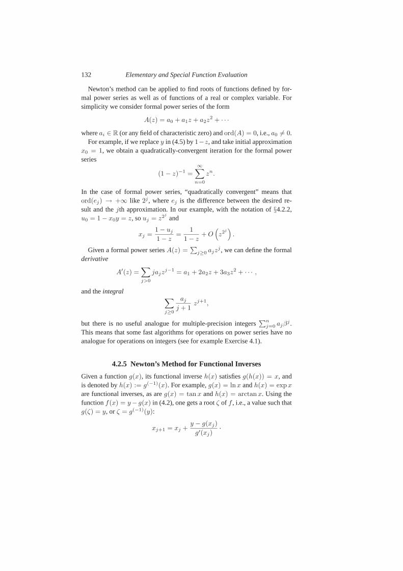
132 Elementary and Special Function Evaluation
Newton’s method can be applied to find roots of functions defined by for-mal power series as well as of functions of a real or complex variable. Forsimplicity we consider formal power series of the form
A(z) = a0 + a1z + a2z2 + · · ·
whereai ∈ R (or any field of characteristic zero) andord(A) = 0, i.e.,a0 6= 0.For example, if we replacey in (4.5) by1−z, and take initial approximation
x0 = 1, we obtain a quadratically-convergent iteration for the formal powerseries
(1 − z)−1 =
∞∑
n=0
zn.
In the case of formal power series, “quadratically convergent” means thatord(ej) → +∞ like 2j , whereej is the difference between the desired re-sult and thejth approximation. In our example, with the notation of§4.2.2,u0 = 1 − x0y = z, souj = z2j
and
xj =1 − uj
1 − z=
1
1 − z+ O
(z2j
).
Given a formal power seriesA(z) =∑
j≥0 ajzj , we can define the formal
derivative
A′(z) =∑
j>0
jajzj−1 = a1 + 2a2z + 3a3z
2 + · · · ,
and theintegral∑
j≥0
aj
j + 1zj+1,
but there is no useful analogue for multiple-precision integers∑n
j=0 ajβj .
This means that some fast algorithms for operations on powerseries have noanalogue for operations on integers (see for example Exercise 4.1).
4.2.5 Newton’s Method for Functional Inverses
Given a functiong(x), its functional inverseh(x) satisfiesg(h(x)) = x, andis denoted byh(x) := g(−1)(x). For example,g(x) = lnx andh(x) = exp x
are functional inverses, as areg(x) = tan x andh(x) = arctan x. Using thefunctionf(x) = y− g(x) in (4.2), one gets a rootζ of f , i.e., a value such thatg(ζ) = y, or ζ = g(−1)(y):
xj+1 = xj +y − g(xj)
g′(xj).
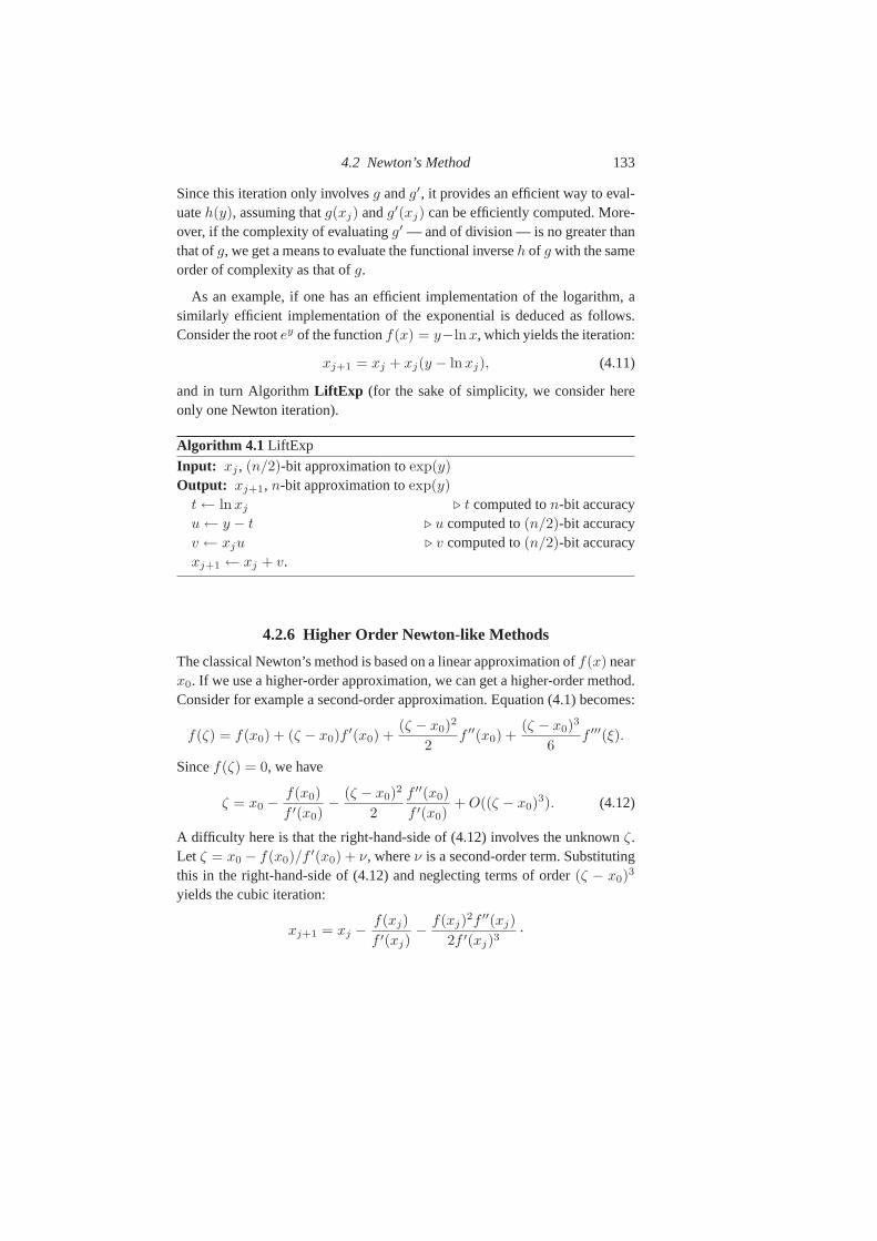
4.2 Newton’s Method 133
Since this iteration only involvesg andg′, it provides an efficient way to eval-uateh(y), assuming thatg(xj) andg′(xj) can be efficiently computed. More-over, if the complexity of evaluatingg′ — and of division — is no greater thanthat ofg, we get a means to evaluate the functional inverseh of g with the sameorder of complexity as that ofg.
As an example, if one has an efficient implementation of the logarithm, asimilarly efficient implementation of the exponential is deduced as follows.Consider the rootey of the functionf(x) = y−lnx, which yields the iteration:
xj+1 = xj + xj(y − lnxj), (4.11)
and in turn AlgorithmLiftExp (for the sake of simplicity, we consider hereonly one Newton iteration).
Algorithm 4.1 LiftExp
Input: xj , (n/2)-bit approximation toexp(y)
Output: xj+1, n-bit approximation toexp(y)
t ← lnxj ⊲ t computed ton-bit accuracyu ← y − t ⊲ u computed to(n/2)-bit accuracyv ← xju ⊲ v computed to(n/2)-bit accuracyxj+1 ← xj + v.
4.2.6 Higher Order Newton-like Methods
The classical Newton’s method is based on a linear approximation of f(x) nearx0. If we use a higher-order approximation, we can get a higher-order method.Consider for example a second-order approximation. Equation (4.1) becomes:
f(ζ) = f(x0) + (ζ − x0)f′(x0) +
(ζ − x0)2
2f ′′(x0) +
(ζ − x0)3
6f ′′′(ξ).
Sincef(ζ) = 0, we have
ζ = x0 −f(x0)
f ′(x0)− (ζ − x0)
2
2
f ′′(x0)
f ′(x0)+ O((ζ − x0)
3). (4.12)
A difficulty here is that the right-hand-side of (4.12) involves the unknownζ.Let ζ = x0 − f(x0)/f ′(x0) + ν, whereν is a second-order term. Substitutingthis in the right-hand-side of (4.12) and neglecting terms of order (ζ − x0)
3
yields the cubic iteration:
xj+1 = xj −f(xj)
f ′(xj)− f(xj)
2f ′′(xj)
2f ′(xj)3.
134 Elementary and Special Function Evaluation
For the computation of the reciprocal (§4.2.2) withf(x) = y−1/x, this yields
xj+1 = xj + xj(1 − xjy) + xj(1 − xjy)2. (4.13)
For the computation ofexp y using functional inversion (§4.2.5), one gets:
xj+1 = xj + xj(y − lnxj) +1
2xj(y − lnxj)
2. (4.14)
These iterations can be obtained in a more systematic way that generalises togive iterations of arbitrarily high order. For the computation of the reciprocal,let εj = 1 − xjy, soxjy = 1 − εj and (assuming|εj | < 1),
1/y = xj/(1 − εj) = xj(1 + εj + ε2j + · · · ).
Truncating after the termεk−1j gives ak-th order iteration
xj+1 = xj(1 + εj + ε2j + · · · + εk−1
j ) (4.15)
for the reciprocal. The casek = 2 corresponds to Newton’s method, and thecasek = 3 is just the iteration (4.13) that we derived above.
Similarly, for the exponential we takeεj = y − lnxj = ln(x/xj), so
x/xj = exp εj =∞∑
m=0
εmj
m!.
Truncating afterk terms gives ak-th order iteration
xj+1 = xj
(k−1∑
m=0
εmj
m!
)(4.16)
for the exponential function. The casek = 2 corresponds to the Newton itera-tion, the casek = 3 is the iteration (4.14) that we derived above, and the casesk > 3 give higher-order Newton-like iterations. For a generalisation to otherfunctions, see Exercises 4.3, 4.6.
4.3 Argument Reduction
Argument reductionis a classical method to improve the efficiency of the eval-uation of mathematical functions. The key idea is to reduce the initial problemto a domain where the function is easier to evaluate. More precisely, givenf
to evaluate atx, one proceeds in three steps:
4.3 Argument Reduction 135
• argument reduction: x is transformed into areduced argumentx′;• evaluation: f is evaluated atx′;• reconstruction: f(x) is computed fromf(x′) using a functional identity.
In some cases the argument reduction or the reconstruction is trivial, for ex-amplex′ = x/2 in radix 2, or f(x) = ±f(x′) (some examples illustrate thisbelow). It might also be that the evaluation step uses a different functiong
instead off ; for examplesin(x + π/2) = cos(x).Unfortunately, argument reduction formulæ do not exist forevery function;
for example, no argument reduction is known for the error function. Argumentreduction is only possible when a functional identity relatesf(x) andf(x′) (org(x) andg(x′)). The elementary functions haveaddition formulaesuch as
exp(x + y) = exp(x) exp(y),
log(xy) = log(x) + log(y),
sin(x + y) = sin(x) cos(y) + cos(x) sin(y),
tan(x + y) =tan(x) + tan(y)
1 − tan(x) tan(y). (4.17)
We use these formulæ to reduce the argument so that power series convergemore rapidly. Usually we takex = y to getdoubling formulaesuch as
exp(2x) = exp(x)2, (4.18)
though occasionallytripling formulaesuch as
sin(3x) = 3 sin(x) − 4 sin3(x)
might be useful. This tripling formula only involves one function (sin), whereasthe doubling formulasin(2x) = 2 sin x cos x involves two functions (sin andcos), but this problem can be overcome: see§4.3.4 and§4.9.1.
We usually distinguish two kinds of argument reduction:
• additive argument reduction, wherex′ = x − kc, for some real constantc and some integerk. This occurs in particular whenf(x) is periodic, forexample for the sine and cosine functions withc = 2π;
• multiplicative argument reduction, wherex′ = x/ck for some real constantc and some integerk. This occurs withc = 2 in the computation ofexp x
when using the doubling formula (4.18): see§4.3.1.
Note that, for a given function, both kinds of argument reduction might beavailable. For example, forsinx, one might either use the tripling formulasin(3x) = 3 sin x − 4 sin3 x, or the additive reductionsin(x + 2kπ) = sin x
that arises from the periodicity ofsin.
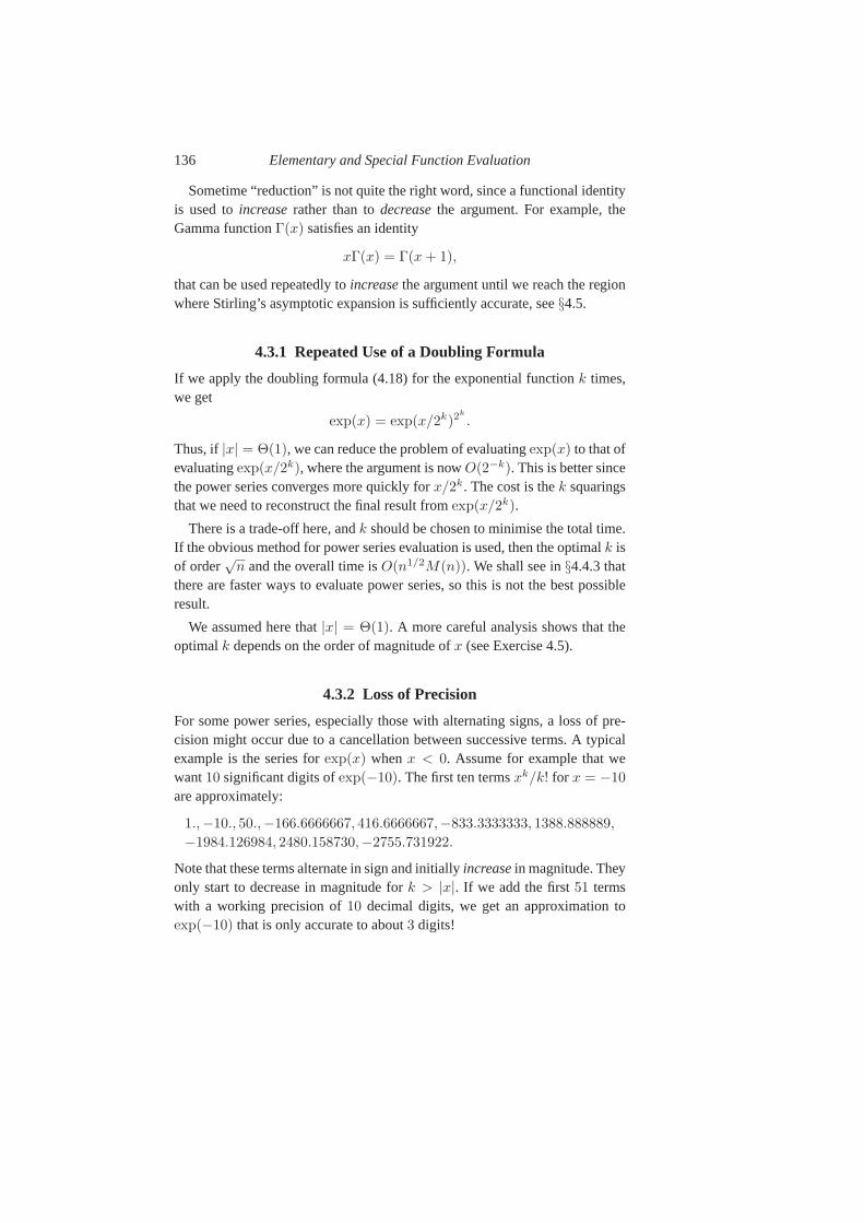
136 Elementary and Special Function Evaluation
Sometime “reduction” is not quite the right word, since a functional identityis used toincreaserather than todecreasethe argument. For example, theGamma functionΓ(x) satisfies an identity
xΓ(x) = Γ(x + 1),
that can be used repeatedly toincreasethe argument until we reach the regionwhere Stirling’s asymptotic expansion is sufficiently accurate, see§4.5.
4.3.1 Repeated Use of a Doubling Formula
If we apply the doubling formula (4.18) for the exponential functionk times,we get
exp(x) = exp(x/2k)2k
.
Thus, if|x| = Θ(1), we can reduce the problem of evaluatingexp(x) to that ofevaluatingexp(x/2k), where the argument is nowO(2−k). This is better sincethe power series converges more quickly forx/2k. The cost is thek squaringsthat we need to reconstruct the final result fromexp(x/2k).
There is a trade-off here, andk should be chosen to minimise the total time.If the obvious method for power series evaluation is used, then the optimalk isof order
√n and the overall time isO(n1/2M(n)). We shall see in§4.4.3 that
there are faster ways to evaluate power series, so this is notthe best possibleresult.
We assumed here that|x| = Θ(1). A more careful analysis shows that theoptimalk depends on the order of magnitude ofx (see Exercise 4.5).
4.3.2 Loss of Precision
For some power series, especially those with alternating signs, a loss of pre-cision might occur due to a cancellation between successiveterms. A typicalexample is the series forexp(x) whenx < 0. Assume for example that wewant10 significant digits ofexp(−10). The first ten termsxk/k! for x = −10
are approximately:
1.,−10., 50.,−166.6666667, 416.6666667,−833.3333333, 1388.888889,
−1984.126984, 2480.158730,−2755.731922.
Note that these terms alternate in sign and initiallyincreasein magnitude. Theyonly start to decrease in magnitude fork > |x|. If we add the first51 termswith a working precision of10 decimal digits, we get an approximation toexp(−10) that is only accurate to about3 digits!
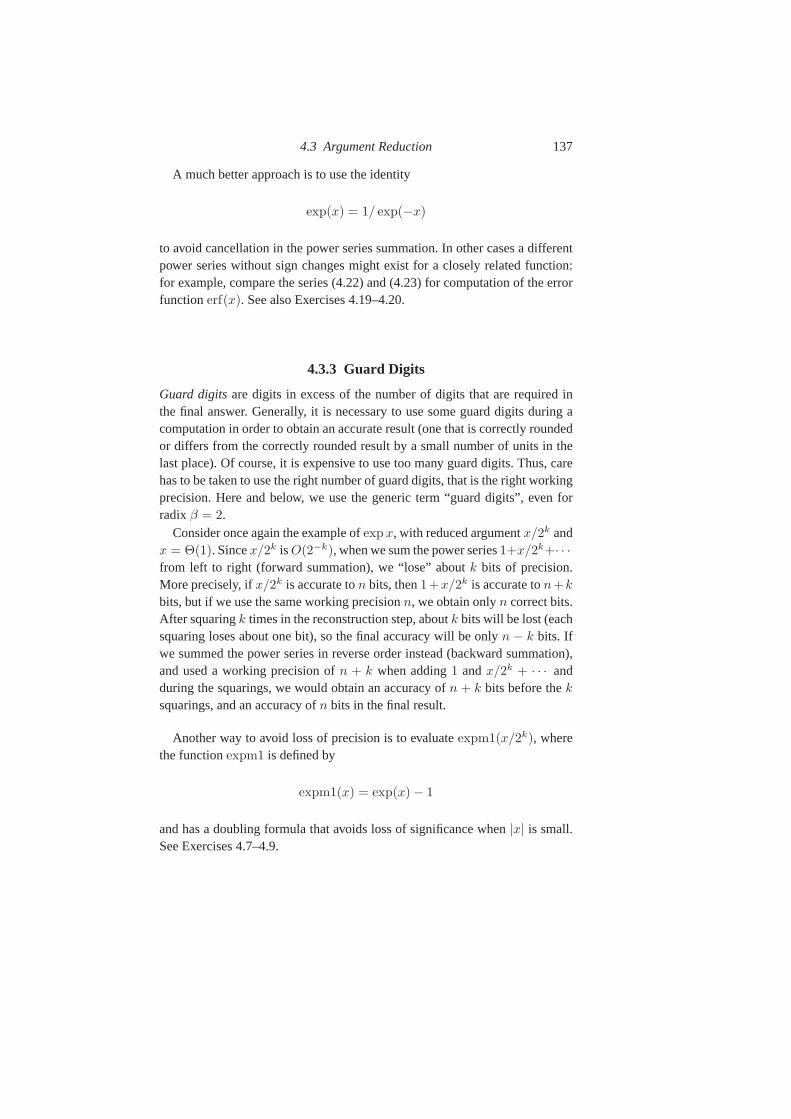
4.3 Argument Reduction 137
A much better approach is to use the identity
exp(x) = 1/ exp(−x)
to avoid cancellation in the power series summation. In other cases a differentpower series without sign changes might exist for a closely related function:for example, compare the series (4.22) and (4.23) for computation of the errorfunctionerf(x). See also Exercises 4.19–4.20.
4.3.3 Guard Digits
Guard digitsare digits in excess of the number of digits that are requiredinthe final answer. Generally, it is necessary to use some guarddigits during acomputation in order to obtain an accurate result (one that is correctly roundedor differs from the correctly rounded result by a small number of units in thelast place). Of course, it is expensive to use too many guard digits. Thus, carehas to be taken to use the right number of guard digits, that isthe right workingprecision. Here and below, we use the generic term “guard digits”, even forradixβ = 2.
Consider once again the example ofexp x, with reduced argumentx/2k andx = Θ(1). Sincex/2k isO(2−k), when we sum the power series1+x/2k+· · ·from left to right (forward summation), we “lose” aboutk bits of precision.More precisely, ifx/2k is accurate ton bits, then1+x/2k is accurate ton+k
bits, but if we use the same working precisionn, we obtain onlyn correct bits.After squaringk times in the reconstruction step, aboutk bits will be lost (eachsquaring loses about one bit), so the final accuracy will be only n − k bits. Ifwe summed the power series in reverse order instead (backward summation),and used a working precision ofn + k when adding1 andx/2k + · · · andduring the squarings, we would obtain an accuracy ofn + k bits before theksquarings, and an accuracy ofn bits in the final result.
Another way to avoid loss of precision is to evaluateexpm1(x/2k), wherethe functionexpm1 is defined by
expm1(x) = exp(x) − 1
and has a doubling formula that avoids loss of significance when |x| is small.See Exercises 4.7–4.9.
138 Elementary and Special Function Evaluation
4.3.4 Doubling versus Tripling
Suppose we want to compute the functionsinh(x) = (ex − e−x)/2. The ob-vious doubling formula forsinh,
sinh(2x) = 2 sinh(x) cosh(x),
involves the auxiliary functioncosh(x) = (ex + e−x)/2. Sincecosh2(x) −sinh2(x) = 1, we could use the doubling formula
sinh(2x) = 2 sinh(x)
√1 + sinh2(x),
but this involves the overhead of computing a square root. This suggests usingthe tripling formula
sinh(3x) = sinh(x)(3 + 4 sinh2(x)). (4.19)
However, it is usually more efficient to do argument reduction via the doublingformula (4.18) forexp, because it takes one multiplication and one squaringto apply the tripling formula, but only two squarings to apply the doublingformula twice (and3 < 22). A drawback is loss of precision, caused by can-cellation in the computation ofexp(x) − exp(−x), when|x| is small. In thiscase it is better to use (see Exercise 4.10)
sinh(x) = (expm1(x) − expm1(−x))/2. (4.20)
See§4.12 for further comments on doubling versus tripling, especially in theFFT range.
4.4 Power Series
Once argument reduction has been applied, where possible (§4.3), one is usu-ally faced with the evaluation of a power series. The elementary and specialfunctions have power series expansions such as:
exp x =∑
j≥0
xj
j!, ln(1 + x) =
∑
j≥0
(−1)jxj+1
j + 1,
arctan x =∑
j≥0
(−1)jx2j+1
2j + 1, sinhx =
∑
j≥0
x2j+1
(2j + 1)!, etc.
This section discusses several techniques to recommend or to avoid. We usethe following notations:x is the evaluation point,n is the desired precision,andd is the number of terms retained in the power series, ord−1 is the degreeof the corresponding polynomial
∑0≤j<d ajx
j .
4.4 Power Series 139
If f(x) is analytic in a neighbourhood of some pointc, an obvious methodto consider for the evaluation off(x) is summation of the Taylor series
f(x) =
d−1∑
j=0
(x − c)j f (j)(c)
j!+ Rd(x, c).
As a simple but instructive example we consider the evaluation of exp(x)
for |x| ≤ 1, using
exp(x) =
d−1∑
j=0
xj
j!+ Rd(x), (4.21)
where|Rd(x)| ≤ |x|d exp(|x|)/d! ≤ e/d!.Using Stirling’s approximation ford!, we see thatd ≥ K(n) ∼ n/ lg n is
sufficient to ensure that|Rd(x)| = O(2−n). Thus, the time required to evaluate(4.21) with Horner’s rule4 is O(nM(n)/ log n).
In practice it is convenient to sum the series in the forward direction(j = 0, 1, . . . , d − 1). The termstj = xj/j! and partial sums
Sj =
j∑
i=0
ti
may be generated by the recurrencetj = xtj−1/j, Sj = Sj−1 + tj , and thesummation terminated when|td| < 2−n/e. Thus, it is not necessary to estimated in advance, as it would be if the series were summed by Horner’s rule in thebackward direction(j = d − 1, d − 2, . . . , 0) (see however Exercise 4.4).
We now consider the effect of rounding errors, under the assumption thatfloating-point operations are correctly rounded, i.e., satisfy
(x op y) = (x op y)(1 + δ),
where|δ| ≤ ε and “op” = “+”, “−”, “×” or “/”. Here ε = 2−n is the “machineprecision” or “working precision”. Lettj be the computed value oftj , etc.Thus
|tj − tj | / |tj | ≤ 2jε + O(ε2)
4 By Horner’s rule(with argumentx) we mean evaluating the polynomials0 =
P
0≤j≤d ajxj of degreed (notd − 1 in this footnote) by the recurrencesd = ad,
sj = aj + sj+1x for j = d − 1, d − 2, . . . , 0. Thussk =P
k≤j≤d ajxj−k. Anevaluation by Horner’s rule takesd additions andd multiplications, and is more efficient thanexplicitly evaluating the individual termsajxj .
140 Elementary and Special Function Evaluation
and using∑d
j=0 tj = Sd ≤ e:
|Sd − Sd| ≤ deε +d∑
j=1
2jε|tj | + O(ε2)
≤ (d + 2)eε + O(ε2) = O(nε).
Thus, to get|Sd−Sd| = O(2−n), it is sufficient thatε = O(2−n/n). In otherwords, we need to work with aboutlg n guard digits. This is not a significantoverhead if (as we assume) the number of digits may vary dynamically. Wecan sum withj increasing (theforwarddirection) or decreasing (thebackwarddirection). A slightly better error bound is obtainable forsummation in thebackward direction, but this method has the disadvantage that the number oftermsd has to be decided in advance (see however Exercise 4.4).
In practice it is inefficient to keep the working precisionε fixed. We canprofitably reduce it when computingtj from tj−1 if |tj−1| is small, withoutsignificantly increasing the error bound. We can also vary the working preci-sion when accumulating the sum, especially if it is computedin the backwarddirection (so the smallest terms are summed first).
It is instructive to consider the effect of relaxing our restriction that|x| ≤ 1.First suppose thatx is large and positive. Since|tj | > |tj−1| whenj < |x|, itis clear that the number of terms required in the sum (4.21) isat least of order|x|. Thus, the method is slow for large|x| (see§4.3 for faster methods in thiscase).
If |x| is large andx is negative, the situation is even worse. From Stirling’sapproximation we have
maxj≥0
|tj | ≃ exp |x|√2π|x|
,
but the result isexp(−|x|), so about2|x|/ log 2 guard digits are required tocompensate for what Lehmer called “catastrophic cancellation” [94]. Sinceexp(x) = 1/ exp(−x), this problem may easily be avoided, but the corre-sponding problem is not always so easily avoided for other analytic functions.
Here is a less trivial example. To compute the error function
erf(x) =2√π
∫ x
0
e−u2
du,
we may use either the power series
erf(x) =2x√π
∞∑
j=0
(−1)j x2j
j!(2j + 1)(4.22)
4.4 Power Series 141
or the (mathematically, but not numerically) equivalent
erf(x) =2xe−x2
√π
∞∑
j=0
2j x2j
1 · 3 · 5 · · · (2j + 1). (4.23)
For small|x|, the series (4.22) is slightly faster than the series (4.23)becausethere is no need to compute an exponential. However, the series (4.23) is prefer-able to (4.22) for moderate|x| because it involves no cancellation. For large|x| neither series is satisfactory, becauseΩ(x2) terms are required, and in thiscase it is preferable to use the asymptotic expansion forerfc(x) = 1 − erf(x):see§4.5. In the borderline region use of the continued fraction (4.40) could beconsidered: see Exercise 4.31.
In the following subsections we consider different methodsto evaluate powerseries. We generally ignore the effect of rounding errors, but the results ob-tained above are typical.
Assumption about the CoefficientsWe assume in this section that we have a power series
∑j≥0 ajx
j whereaj+δ/aj is a rational functionR(j) of j, and hence it is easy to evaluatea0, a1, a2, . . . sequentially. Hereδ is a fixed positive constant, usually1 or2. For example, in the case ofexp x, we haveδ = 1 and
aj+1
aj=
j!
(j + 1)!=
1
j + 1.
Our assumptions cover the common case of hypergeometric functions. For themore general case of holonomic functions, see§4.9.2.
In common cases where our assumption is invalid, other good methods areavailable to evaluate the function. For example,tan x does not satisfy our as-sumption (the coefficients in its Taylor series are calledtangent numbersandare related to Bernoulli numbers – see§4.7.2), but to evaluatetan x we canuse Newton’s method on the inverse function (arctan, which does satisfy ourassumptions – see§4.2.5), or we can usetan x = sin x/ cos x.
The Radius of ConvergenceIf the elementary function is an entire function (e.g.,exp, sin) then the powerseries converges in the whole complex plane. In this case thedegree of thedenominator ofR(j) = aj+1/aj is greater than that of the numerator.
In other cases (such asln, arctan) the function is not entire. The powerseries only converges in a disk because the function has a singularity on theboundary of this disk. In factln(x) has a singularity at the origin, which is
142 Elementary and Special Function Evaluation
why we consider the power series forln(1 + x). This power series has radiusof convergence 1.
Similarly, the power series forarctan(x) has radius of convergence 1 be-causearctan(x) has singularities on the unit circle (at±i) even though it isuniformly bounded for all realx.
4.4.1 Direct Power Series Evaluation
Suppose that we want to evaluate a power series∑
j≥0 ajxj at a given argu-
mentx. Using periodicity (in the cases ofsin, cos) and/or argument reductiontechniques (§4.3), we can often ensure that|x| is sufficiently small. Thus, letus assume that|x| ≤ 1/2 and that the radius of convergence of the series is atleast 1.
As above, assume thataj+δ/aj is a rational function ofj, and hence easyto evaluate. For simplicity we consider only the caseδ = 1. To sum the serieswith errorO(2−n) it is sufficient to taken + O(1) terms, so the time requiredis O(nM(n)). If the function is entire, then the series converges fasterand thetime is reduced toO(nM(n)/(log n)). However, we can do much better bycarrying the argument reduction further, as demonstrated in the next section.
4.4.2 Power Series With Argument Reduction
Consider the evaluation ofexp(x). By applying argument reductionk + O(1)
times, we can ensure that the argumentx satisfies|x| < 2−k. Then, to obtainn-bit accuracy we only need to sumO(n/k) terms of the power series. Assumingthat a step of argument reduction isO(M(n)), which is true for the elementaryfunctions, the total cost isO((k+n/k)M(n)). Indeed, the argument reductionand/or reconstruction requiresO(k) steps ofO(M(n)), and the evaluation ofthe power series of ordern/k costs(n/k)M(n); so choosingk ∼ n1/2 givescost
O(n1/2M(n)
).
For example, our comments apply to the evaluation ofexp(x) using
exp(x) = exp(x/2)2,
to log1p(x) = ln(1 + x) using
log1p(x) = 2 log1p
(x
1 +√
1 + x
),
4.4 Power Series 143
and toarctan(x) using
arctan x = 2arctan
(x
1 +√
1 + x2
).
Note that in the last two cases each step of the argument reduction requiresa square root, but this can be done with costO(M(n)) by Newton’s method(§3.5). Thus in all three cases the overall cost isO(n1/2M(n)), although theimplicit constant might be smaller forexp than forlog1p or arctan. See Exer-cises 4.8–4.9.
Using SymmetriesA not-so-well-known idea is to evaluateln(1 + x) using the power series
ln
(1 + y
1 − y
)= 2
∑
j≥0
y2j+1
2j + 1
with y defined by(1 + y)/(1 − y) = 1 + x, i.e.,y = x/(2 + x). This saveshalf the terms and also reduces the argument, sincey < x/2 if x > 0. Un-fortunately this nice idea can be applied only once. For a related example, seeExercise 4.11.
4.4.3 Rectangular Series Splitting
Once we determine how many terms in the power series are required for thedesired accuracy, the problem reduces to evaluating a truncated power series,i.e., a polynomial.
Let P (x) =∑
0≤j<d ajxj be the polynomial that we want to evaluate,
deg(P ) < d. In the general casex is a floating-point number ofn bits, andwe aim at an accuracy ofn bits for P (x). However the coefficientsaj , ortheir ratiosR(j) = aj+1/aj , are usually small integers or rational numbers ofO(log n) bits. A scalar multiplicationinvolves one coefficientaj and the vari-ablex (or more generally ann-bit floating-point number), whereas anonscalarmultiplication involves two powers ofx (or more generally twon-bit floating-point numbers). Scalar multiplications are cheaper because theaj are smallrationals of sizeO(log n), whereasx and its powers generally haveΘ(n) bits.It is possible to evaluateP (x) with O(
√n) nonscalar multiplications (plus
O(n) scalar multiplications andO(n) additions, usingO(√
n) storage). Thesame idea applies, more generally, to evaluation of hypergeometric functions.
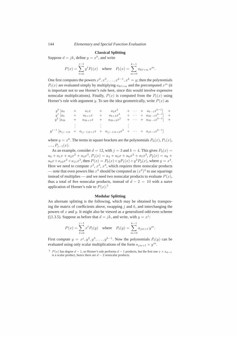
144 Elementary and Special Function Evaluation
Classical SplittingSupposed = jk, definey = xk, and write
P (x) =
j−1∑
ℓ=0
yℓPℓ(x) where Pℓ(x) =k−1∑
m=0
akℓ+m xm.
One first computes the powersx2, x3, . . . , xk−1, xk = y; then the polynomialsPℓ(x) are evaluated simply by multiplyingakℓ+m and the precomputedxm (itis important not to use Horner’s rule here, since this would involve expensivenonscalar multiplications). Finally,P (x) is computed from thePℓ(x) usingHorner’s rule with argumenty. To see the idea geometrically, writeP (x) as
y0 [a0 + a1x + a2x2 + · · · + ak−1x
k−1] +y1 [ak + ak+1x + ak+2x
2 + · · · + a2k−1xk−1] +
y2 [a2k + a2k+1x + a2k+2x2 + · · · + a3k−1x
k−1] +...
......
yj−1 [a(j−1)k + a(j−1)k+1x + a(j−1)k+2x2 + · · · + ajk−1x
k−1]
wherey = xk. The terms in square brackets are the polynomialsP0(x), P1(x),. . . ,Pj−1(x).
As an example, considerd = 12, with j = 3 andk = 4. This givesP0(x) =
a0 + a1x + a2x2 + a3x
3, P1(x) = a4 + a5x + a6x2 + a7x
3, P2(x) = a8 +
a9x+a10x2 +a11x
3, thenP (x) = P0(x)+yP1(x)+y2P2(x), wherey = x4.Here we need to computex2, x3, x4, which requires three nonscalar products— note that even powers likex4 should be computed as(x2)2 to use squaringsinstead of multiplies — and we need two nonscalar products toevaluateP (x),thus a total of five nonscalar products, instead ofd − 2 = 10 with a naiveapplication of Horner’s rule toP (x).5
Modular SplittingAn alternate splitting is the following, which may be obtained by transpos-ing the matrix of coefficients above, swappingj andk, and interchanging thepowers ofx andy. It might also be viewed as a generalized odd-even scheme(§1.3.5). Suppose as before thatd = jk, and write, withy = xj :
P (x) =
j−1∑
ℓ=0
xℓPℓ(y) where Pℓ(y) =
k−1∑
m=0
ajm+ℓ ym.
First computey = xj , y2, y3, . . . , yk−1. Now the polynomialsPℓ(y) can beevaluated using only scalar multiplications of the formajm+ℓ × ym.
5 P (x) has degreed − 1, so Horner’s rule performsd − 1 products, but the first onex × ad−1
is a scalar product, hence there ared − 2 nonscalar products.
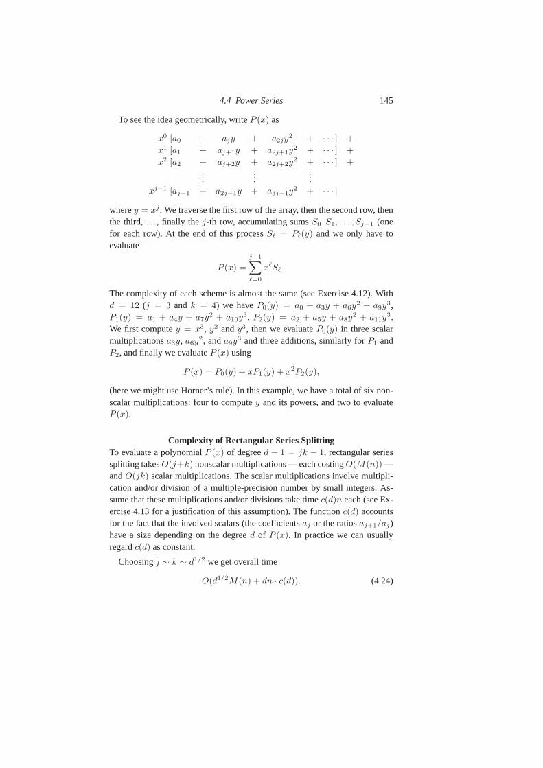
4.4 Power Series 145
To see the idea geometrically, writeP (x) as
x0 [a0 + ajy + a2jy2 + · · · ] +
x1 [a1 + aj+1y + a2j+1y2 + · · · ] +
x2 [a2 + aj+2y + a2j+2y2 + · · · ] +
......
...xj−1 [aj−1 + a2j−1y + a3j−1y
2 + · · · ]
wherey = xj . We traverse the first row of the array, then the second row, thenthe third,. . ., finally the j-th row, accumulating sumsS0, S1, . . . , Sj−1 (onefor each row). At the end of this processSℓ = Pℓ(y) and we only have toevaluate
P (x) =
j−1∑
ℓ=0
xℓSℓ .
The complexity of each scheme is almost the same (see Exercise 4.12). Withd = 12 (j = 3 andk = 4) we haveP0(y) = a0 + a3y + a6y
2 + a9y3,
P1(y) = a1 + a4y + a7y2 + a10y
3, P2(y) = a2 + a5y + a8y2 + a11y
3.We first computey = x3, y2 andy3, then we evaluateP0(y) in three scalarmultiplicationsa3y, a6y
2, anda9y3 and three additions, similarly forP1 and
P2, and finally we evaluateP (x) using
P (x) = P0(y) + xP1(y) + x2P2(y),
(here we might use Horner’s rule). In this example, we have a total of six non-scalar multiplications: four to computey and its powers, and two to evaluateP (x).
Complexity of Rectangular Series SplittingTo evaluate a polynomialP (x) of degreed − 1 = jk − 1, rectangular seriessplitting takesO(j+k) nonscalar multiplications — each costingO(M(n)) —andO(jk) scalar multiplications. The scalar multiplications involve multipli-cation and/or division of a multiple-precision number by small integers. As-sume that these multiplications and/or divisions take timec(d)n each (see Ex-ercise 4.13 for a justification of this assumption). The function c(d) accountsfor the fact that the involved scalars (the coefficientsaj or the ratiosaj+1/aj)have a size depending on the degreed of P (x). In practice we can usuallyregardc(d) as constant.
Choosingj ∼ k ∼ d1/2 we get overall time
O(d1/2M(n) + dn · c(d)). (4.24)

146 Elementary and Special Function Evaluation
If d is of the same order as the precisionn of x, this is not an improvementon the boundO(n1/2M(n)) that we obtained already by argument reductionand power series evaluation (§4.4.2). However, we can do argument reductionbefore applying rectangular series splitting. Assuming that c(n) = O(1) (seeExercise 4.14 for a detailed analysis), the total complexity is:
T (n) = O(n
dM(n) + d1/2M(n) + dn
),
where the extra(n/d)M(n) term comes from argument reduction and/or re-construction. Which term dominates? There are two cases:
1. M(n) ≫ n4/3. Here the minimum is obtained when the first two terms— argument reduction/reconstruction and nonscalar multiplications — areequal, i.e., ford ∼ n2/3, which yieldsT (n) = O(n1/3M(n)). This caseapplies if we use classical or Karatsuba multiplication, since lg 3 > 4/3,and similarly for Toom-Cook3-, 4-, 5-, or 6-way multiplication (but not7-way, sincelog7 13 < 4/3). In this caseT (n) ≫ n5/3.
2. M(n) ≪ n4/3. Here the minimum is obtained when the first and the lastterms — argument reduction/reconstruction and scalar multiplications —are equal. The optimal value ofd is then
√M(n), and we get an improved
boundΘ(n√
M(n)) ≫ n3/2. We can not approach theO(n1+ε) that isachievable with AGM-based methods (if applicable) – see§4.8.
4.5 Asymptotic Expansions
Often it is necessary to use different methods to evaluate a special function indifferent parts of its domain. For example, the exponentialintegral6
E1(x) =
∫ ∞
x
exp(−u)
udu (4.25)
is defined for allx > 0. However, the power series
E1(x) + γ + lnx =∞∑
j=1
(−1)j−1xj
j!j(4.26)
is unsatisfactory as a means of evaluatingE1(x) for large positivex, for thereasons discussed in§4.4 in connection with the power series (4.22) forerf(x),
6 E1(x) andEi(x) = PVR x−∞
(exp(t)/t) dt are both called “exponential integrals”. Closely
related is the “logarithmic integral”li(x) = Ei(ln x) = PVR x0 (1/ ln t) dt. Here the integrals
PVR
· · · should be interpreted as Cauchy principal values if there isa singularity in the rangeof integration. The power series (4.26) is valid forx ∈ C if | arg x| < π (see Exercise 4.16).

4.5 Asymptotic Expansions 147
or the power series forexp(x) (x negative). For sufficiently large positivex itis preferable to use
ex E1(x) =k∑
j=1
(j − 1)!(−1)j−1
xj+ Rk(x), (4.27)
where
Rk(x) = k! (−1)k exp(x)
∫ ∞
x
exp(−u)
uk+1du. (4.28)
Note that
|Rk(x)| <k!
xk+1,
so
limx→+∞
Rk(x) = 0,
but limk→∞ Rk(x) does not exist. In other words, the series∞∑
j=1
(j − 1)! (−1)j−1
xj
is divergent. In such cases we call this anasymptotic seriesand write
ex E1(x) ∼∑
j>0
(j − 1)!(−1)j−1
xj. (4.29)
Although they do not generally converge, asymptotic seriesare very useful.Often (though not always!) the error is bounded by the last term taken in theseries (or by the first term omitted). Also, when the terms in the asymptoticseries alternate in sign, it can often be shown that the true value lies betweentwo consecutive approximations obtained by summing the series with (say)kandk + 1 terms. For example, this is true for the series (4.29) above,providedx is real and positive.
Whenx is large and positive, the relative error attainable by using (4.27)with k = ⌊x⌋ is O(x1/2 exp(−x)), because
|Rk(k)| ≤ k!/kk+1 = O(k−1/2 exp(−k)) (4.30)
and the leading term on the right side of (4.27) is1/x. Thus, the asymp-totic series may be used to evaluateE1(x) to precisionn wheneverx >
n ln 2+O(ln n). More precise estimates can be obtained by using a version ofStirling’s approximation with error bounds, for example
(k
e
)k √2πk < k! <
(k
e
)k √2πk exp
(1
12k
).
148 Elementary and Special Function Evaluation
If x is too small for the asymptotic approximation to be sufficiently accurate,we can avoid the problem of cancellation in the power series (4.26) by thetechnique of Exercise 4.19. However, the asymptotic approximation is fasterand hence is preferable whenever it is sufficiently accurate.
Examples where asymptotic expansions are useful include the evaluation oferfc(x), Γ(x), Bessel functions,etc.We discuss some of these below.
Asymptotic expansions often arise when the convergence of series is accel-erated by the Euler-Maclaurin sum formula.7 For example, Euler’s constantγ
is defined by
γ = limN→∞
(HN − lnN) , (4.31)
whereHN =∑
1≤j≤N 1/j is a harmonic number. However, Eqn. (4.31) con-verges slowly, so to evaluateγ accurately we need to accelerate the conver-gence. This can be done using the Euler-Maclaurin formula. The idea is tosplit the sumHN into two parts:
HN = Hp−1 +N∑
j=p
1
j.
We approximate the second sum using the Euler-Maclaurin formula7 witha = p, b = N , f(x) = 1/x, then letN → +∞. The result is
γ ∼ Hp − ln p +∑
k≥1
B2k
2kp−2k. (4.32)
If p and the number of terms in the asymptotic expansion are chosen judi-ciously, this gives a good algorithm for computingγ (though not the best algo-rithm: see§4.12 for a faster algorithm that uses properties of Bessel functions).
Here is another example. The Riemann zeta-functionζ(s) is defined fors ∈ C, ℜ(s) > 1, by
ζ(s) =∞∑
j=1
j−s, (4.33)
and by analytic continuation for others 6= 1. ζ(s) may be evaluated to any
7 The Euler-Maclaurin sum formula is a way of expressing the difference between a sum andan integral as an asymptotic expansion. For example, assuming thata ∈ Z, b ∈ Z, a ≤ b, andf(x) satisfies certain conditions, one form of the formula is
X
a≤k≤b
f(k) −
Z b
af(x) dx ∼
f(a) + f(b)
2+
X
k≥1
B2k
(2k)!
“
f (2k−1)(b) − f (2k−1)(a)”
.
Often we can letb → +∞ and omit the terms involvingb on the right-hand-side. For moreinformation see§4.12.
4.5 Asymptotic Expansions 149
desired precision ifm andp are chosen large enough in the Euler-Maclaurinformula
ζ(s) =
p−1∑
j=1
j−s +p−s
2+
p1−s
s − 1+
m∑
k=1
Tk,p(s) + Em,p(s), (4.34)
where
Tk,p(s) =B2k
(2k)!p1−s−2k
2k−2∏
j=0
(s + j), (4.35)
|Em,p(s)| < |Tm+1,p(s) (s + 2m + 1)/(σ + 2m + 1)|, (4.36)
m ≥ 0, p ≥ 1, σ = ℜ(s) > −(2m + 1), and theB2k are Bernoulli numbers.In arbitrary-precision computations we must be able to compute as many
terms of an asymptotic expansion as are required to give the desired accuracy.It is easy to see that, ifm in (4.34) is bounded as the precisionn goes to∞, thenp has to increase as an exponential function ofn. To evaluateζ(s)
from (4.34) to precisionn in time polynomial inn, bothm andp must tend toinfinity with n. Thus, the Bernoulli numbersB2, . . . , B2m can not be stored ina table of fixed size,8 but must be computed when needed (see§4.7). For thisreason we can not use asymptotic expansions when the generalform of thecoefficients is unknown or the coefficients are too difficult to evaluate. Oftenthere is a related expansion with known and relatively simple coefficients. Forexample, the asymptotic expansion (4.38) forln Γ(x) has coefficients related tothe Bernoulli numbers, like the expansion (4.34) forζ(s), and thus is simpler toimplement than Stirling’s asymptotic expansion forΓ(x) (see Exercise 4.42).
Consider the computation of the error functionerf(x). As seen in§4.4, theseries (4.22) and (4.23) are not satisfactory for large|x|, since they requireΩ(x2) terms. For example, to evaluateerf(1000) with an accuracy of six digits,Eqn. (4.22) requires at least2 718 279 terms! Instead, we may use an asymp-totic expansion. The complementary error functionerfc(x) = 1 − erf(x) sat-isfies
erfc(x) ∼ e−x2
x√
π
k∑
j=0
(−1)j (2j)!
j!(2x)−2j , (4.37)
with the error bounded in absolute value by the next term and of the same sign.In the casex = 1000, the term forj = 1 of the sum equals−0.5 × 10⁻⁶; thus
8 In addition, we would have to store them as exact rationals, taking∼ m2 lg m bits of storage,since a floating-point representation would not be convenient unless the target precisionnwere known in advance. See§4.7.2 and Exercise 4.37.
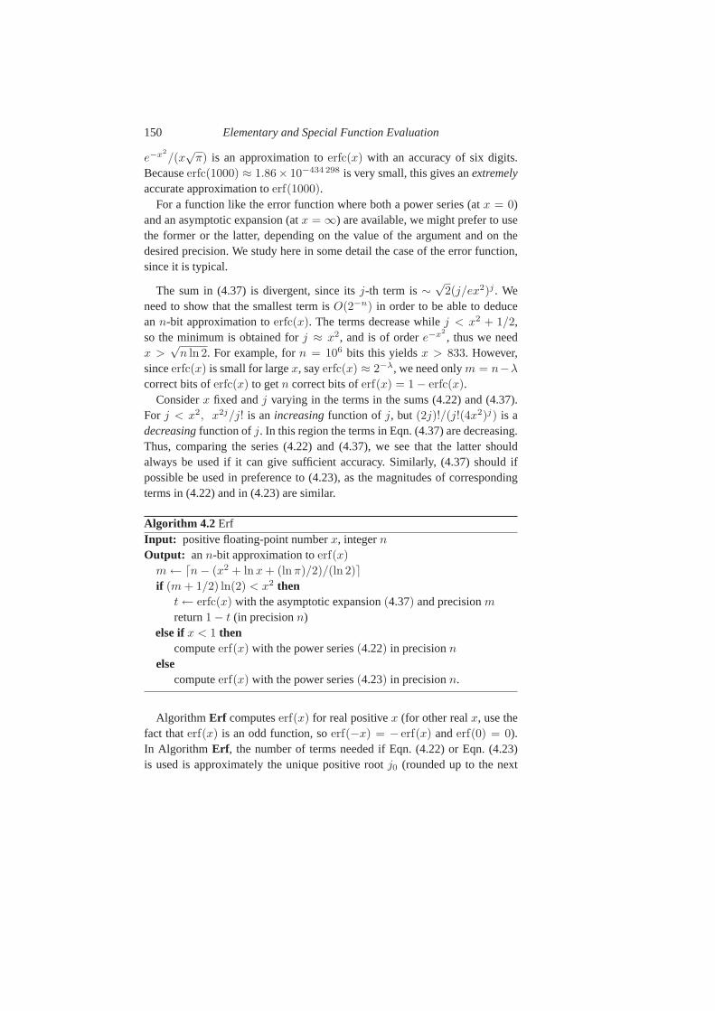
150 Elementary and Special Function Evaluation
e−x2
/(x√
π) is an approximation toerfc(x) with an accuracy of six digits.Becauseerfc(1000) ≈ 1.86× 10−434 298 is very small, this gives anextremelyaccurate approximation toerf(1000).
For a function like the error function where both a power series (atx = 0)and an asymptotic expansion (atx = ∞) are available, we might prefer to usethe former or the latter, depending on the value of the argument and on thedesired precision. We study here in some detail the case of the error function,since it is typical.
The sum in (4.37) is divergent, since itsj-th term is∼√
2(j/ex2)j . Weneed to show that the smallest term isO(2−n) in order to be able to deduceann-bit approximation toerfc(x). The terms decrease whilej < x2 + 1/2,so the minimum is obtained forj ≈ x2, and is of ordere−x2
, thus we needx >
√n ln 2. For example, forn = 106 bits this yieldsx > 833. However,
sinceerfc(x) is small for largex, sayerfc(x) ≈ 2−λ, we need onlym = n−λ
correct bits oferfc(x) to getn correct bits oferf(x) = 1 − erfc(x).Considerx fixed andj varying in the terms in the sums (4.22) and (4.37).
For j < x2, x2j/j! is an increasingfunction of j, but (2j)!/(j!(4x2)j) is adecreasingfunction ofj. In this region the terms in Eqn. (4.37) are decreasing.Thus, comparing the series (4.22) and (4.37), we see that thelatter shouldalways be used if it can give sufficient accuracy. Similarly,(4.37) should ifpossible be used in preference to (4.23), as the magnitudes of correspondingterms in (4.22) and in (4.23) are similar.
Algorithm 4.2 ErfInput: positive floating-point numberx, integernOutput: ann-bit approximation toerf(x)
m ← ⌈n − (x2 + lnx + (lnπ)/2)/(ln 2)⌉if (m + 1/2) ln(2) < x2 then
t ← erfc(x) with the asymptotic expansion(4.37) and precisionmreturn1 − t (in precisionn)
else ifx < 1 thencomputeerf(x) with the power series(4.22) in precisionn
elsecomputeerf(x) with the power series(4.23) in precisionn.
Algorithm Erf computeserf(x) for real positivex (for other realx, use thefact thaterf(x) is an odd function, soerf(−x) = − erf(x) anderf(0) = 0).In Algorithm Erf , the number of terms needed if Eqn. (4.22) or Eqn. (4.23)is used is approximately the unique positive rootj0 (rounded up to the next
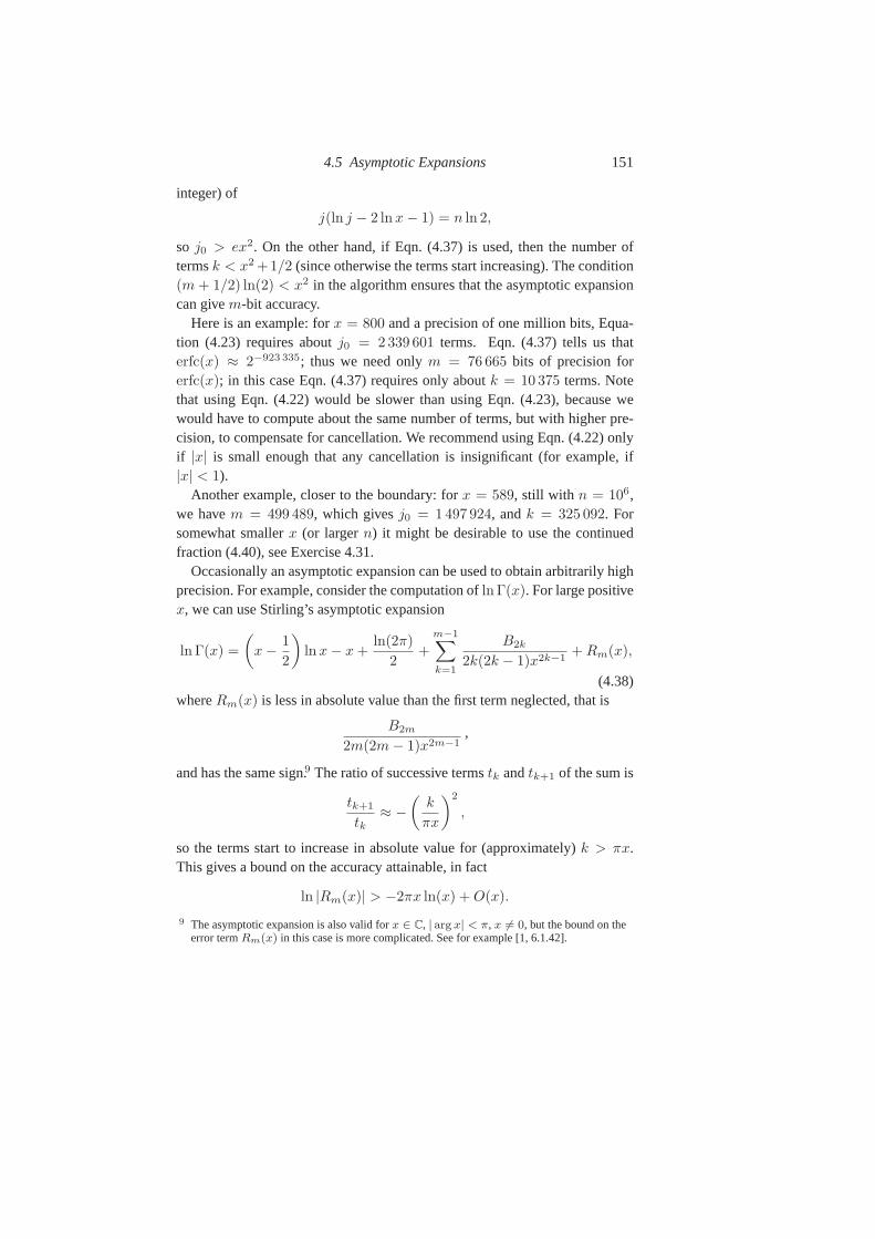
4.5 Asymptotic Expansions 151
integer) of
j(ln j − 2 ln x − 1) = n ln 2,
so j0 > ex2. On the other hand, if Eqn. (4.37) is used, then the number oftermsk < x2 +1/2 (since otherwise the terms start increasing). The condition(m + 1/2) ln(2) < x2 in the algorithm ensures that the asymptotic expansioncan givem-bit accuracy.
Here is an example: forx = 800 and a precision of one million bits, Equa-tion (4.23) requires aboutj0 = 2339 601 terms. Eqn. (4.37) tells us thaterfc(x) ≈ 2−923 335; thus we need onlym = 76 665 bits of precision forerfc(x); in this case Eqn. (4.37) requires only aboutk = 10 375 terms. Notethat using Eqn. (4.22) would be slower than using Eqn. (4.23), because wewould have to compute about the same number of terms, but withhigher pre-cision, to compensate for cancellation. We recommend usingEqn. (4.22) onlyif |x| is small enough that any cancellation is insignificant (for example, if|x| < 1).
Another example, closer to the boundary: forx = 589, still with n = 106,we havem = 499 489, which givesj0 = 1497 924, andk = 325 092. Forsomewhat smallerx (or largern) it might be desirable to use the continuedfraction (4.40), see Exercise 4.31.
Occasionally an asymptotic expansion can be used to obtain arbitrarily highprecision. For example, consider the computation ofln Γ(x). For large positivex, we can use Stirling’s asymptotic expansion
ln Γ(x) =
(x − 1
2
)lnx − x +
ln(2π)
2+
m−1∑
k=1
B2k
2k(2k − 1)x2k−1+ Rm(x),
(4.38)whereRm(x) is less in absolute value than the first term neglected, that is
B2m
2m(2m − 1)x2m−1,
and has the same sign.9 The ratio of successive termstk andtk+1 of the sum is
tk+1
tk≈ −
(k
πx
)2
,
so the terms start to increase in absolute value for (approximately)k > πx.This gives a bound on the accuracy attainable, in fact
ln |Rm(x)| > −2πx ln(x) + O(x).
9 The asymptotic expansion is also valid forx ∈ C, | arg x| < π, x 6= 0, but the bound on theerror termRm(x) in this case is more complicated. See for example [1, 6.1.42].
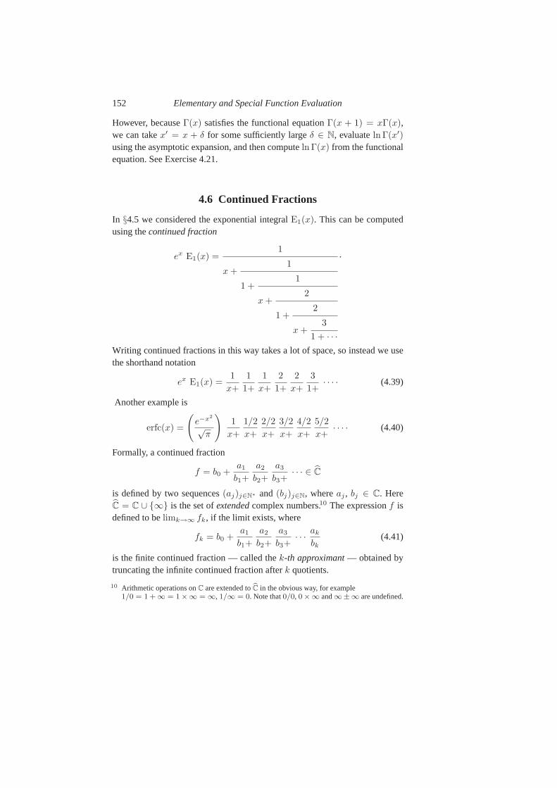
152 Elementary and Special Function Evaluation
However, becauseΓ(x) satisfies the functional equationΓ(x + 1) = xΓ(x),we can takex′ = x + δ for some sufficiently largeδ ∈ N, evaluateln Γ(x′)using the asymptotic expansion, and then computeln Γ(x) from the functionalequation. See Exercise 4.21.
4.6 Continued Fractions
In §4.5 we considered the exponential integralE1(x). This can be computedusing thecontinued fraction
ex E1(x) =1
x +1
1 +1
x +2
1 +2
x +3
1 + · · ·
.
Writing continued fractions in this way takes a lot of space, so instead we usethe shorthand notation
ex E1(x) =1
x+
1
1+
1
x+
2
1+
2
x+
3
1+· · · · (4.39)
Another example is
erfc(x) =
(e−x2
√π
)1
x+
1/2
x+
2/2
x+
3/2
x+
4/2
x+
5/2
x+· · · · (4.40)
Formally, a continued fraction
f = b0 +a1
b1+
a2
b2+
a3
b3+· · · ∈ C
is defined by two sequences(aj)j∈N∗ and(bj)j∈N, whereaj , bj ∈ C. HereC = C ∪ ∞ is the set ofextendedcomplex numbers.10 The expressionf isdefined to belimk→∞ fk, if the limit exists, where
fk = b0 +a1
b1+
a2
b2+
a3
b3+· · · ak
bk(4.41)
is the finite continued fraction — called thek-th approximant— obtained bytruncating the infinite continued fraction afterk quotients.
10 Arithmetic operations onC are extended tobC in the obvious way, for example1/0 = 1 + ∞ = 1 ×∞ = ∞, 1/∞ = 0. Note that0/0, 0 ×∞ and∞±∞ are undefined.
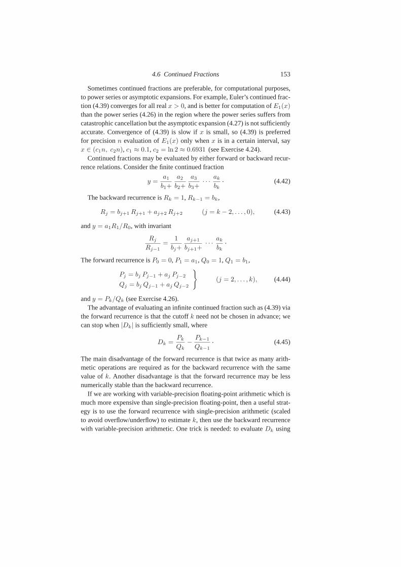
4.6 Continued Fractions 153
Sometimes continued fractions are preferable, for computational purposes,to power series or asymptotic expansions. For example, Euler’s continued frac-tion (4.39) converges for all realx > 0, and is better for computation ofE1(x)
than the power series (4.26) in the region where the power series suffers fromcatastrophic cancellation but the asymptotic expansion (4.27) is not sufficientlyaccurate. Convergence of (4.39) is slow ifx is small, so (4.39) is preferredfor precisionn evaluation ofE1(x) only whenx is in a certain interval, sayx ∈ (c1n, c2n), c1 ≈ 0.1, c2 = ln 2 ≈ 0.6931 (see Exercise 4.24).
Continued fractions may be evaluated by either forward or backward recur-rence relations. Consider the finite continued fraction
y =a1
b1+
a2
b2+
a3
b3+· · · ak
bk
. (4.42)
The backward recurrence isRk = 1, Rk−1 = bk,
Rj = bj+1 Rj+1 + aj+2 Rj+2 (j = k − 2, . . . , 0), (4.43)
andy = a1R1/R0, with invariant
Rj
Rj−1=
1
bj+
aj+1
bj+1+· · · ak
bk
.
The forward recurrence isP0 = 0, P1 = a1, Q0 = 1, Q1 = b1,
Pj = bj Pj−1 + aj Pj−2
Qj = bj Qj−1 + aj Qj−2
(j = 2, . . . , k), (4.44)
andy = Pk/Qk (see Exercise 4.26).The advantage of evaluating an infinite continued fraction such as (4.39) via
the forward recurrence is that the cutoffk need not be chosen in advance; wecan stop when|Dk| is sufficiently small, where
Dk =Pk
Qk− Pk−1
Qk−1
. (4.45)
The main disadvantage of the forward recurrence is that twice as many arith-metic operations are required as for the backward recurrence with the samevalue ofk. Another disadvantage is that the forward recurrence may belessnumerically stable than the backward recurrence.
If we are working with variable-precision floating-point arithmetic which ismuch more expensive than single-precision floating-point,then a useful strat-egy is to use the forward recurrence with single-precision arithmetic (scaledto avoid overflow/underflow) to estimatek, then use the backward recurrencewith variable-precision arithmetic. One trick is needed: to evaluateDk using
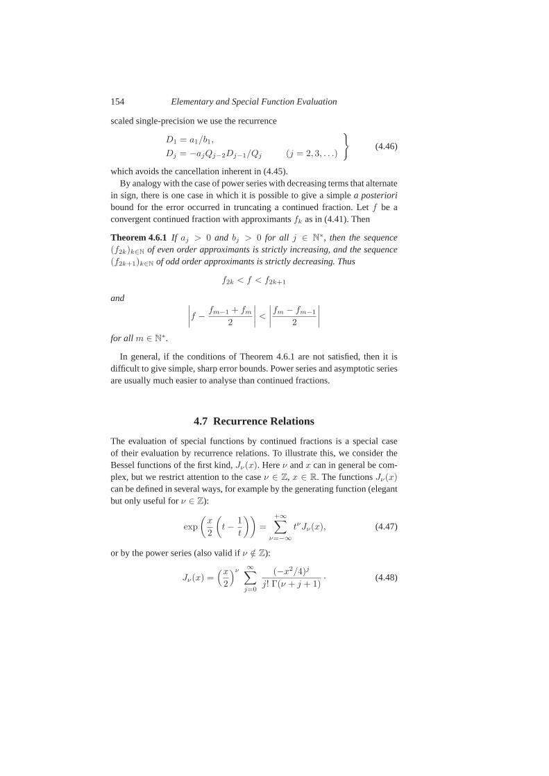
154 Elementary and Special Function Evaluation
scaled single-precision we use the recurrence
D1 = a1/b1,
Dj = −ajQj−2Dj−1/Qj (j = 2, 3, . . .)
(4.46)
which avoids the cancellation inherent in (4.45).By analogy with the case of power series with decreasing terms that alternate
in sign, there is one case in which it is possible to give a simple a posterioribound for the error occurred in truncating a continued fraction. Let f be aconvergent continued fraction with approximantsfk as in (4.41). Then
Theorem 4.6.1 If aj > 0 and bj > 0 for all j ∈ N∗, then the sequence(f2k)k∈N of even order approximants is strictly increasing, and the sequence(f2k+1)k∈N of odd order approximants is strictly decreasing. Thus
f2k < f < f2k+1
and ∣∣∣∣f − fm−1 + fm
2
∣∣∣∣ <
∣∣∣∣fm − fm−1
2
∣∣∣∣
for all m ∈ N∗.
In general, if the conditions of Theorem 4.6.1 are not satisfied, then it isdifficult to give simple, sharp error bounds. Power series and asymptotic seriesare usually much easier to analyse than continued fractions.
4.7 Recurrence Relations
The evaluation of special functions by continued fractionsis a special caseof their evaluation by recurrence relations. To illustratethis, we consider theBessel functions of the first kind,Jν(x). Hereν andx can in general be com-plex, but we restrict attention to the caseν ∈ Z, x ∈ R. The functionsJν(x)
can be defined in several ways, for example by the generating function (elegantbut only useful forν ∈ Z):
exp
(x
2
(t − 1
t
))=
+∞∑
ν=−∞tνJν(x), (4.47)
or by the power series (also valid ifν /∈ Z):
Jν(x) =(x
2
)ν ∞∑
j=0
(−x2/4)j
j! Γ(ν + j + 1). (4.48)
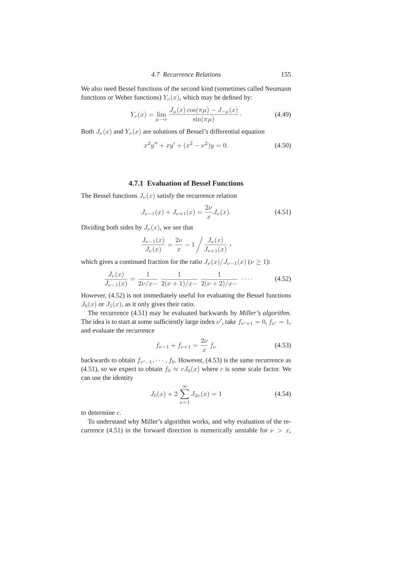
4.7 Recurrence Relations 155
We also need Bessel functions of the second kind (sometimes called Neumannfunctions or Weber functions)Yν(x), which may be defined by:
Yν(x) = limµ→ν
Jµ(x) cos(πµ) − J−µ(x)
sin(πµ). (4.49)
BothJν(x) andYν(x) are solutions of Bessel’s differential equation
x2y′′ + xy′ + (x2 − ν2)y = 0. (4.50)
4.7.1 Evaluation of Bessel Functions
The Bessel functionsJν(x) satisfy the recurrence relation
Jν−1(x) + Jν+1(x) =2ν
xJν(x). (4.51)
Dividing both sides byJν(x), we see that
Jν−1(x)
Jν(x)=
2ν
x− 1
/Jν(x)
Jν+1(x),
which gives a continued fraction for the ratioJν(x)/Jν−1(x) (ν ≥ 1):
Jν(x)
Jν−1(x)=
1
2ν/x−1
2(ν + 1)/x−1
2(ν + 2)/x− · · · · (4.52)
However, (4.52) is not immediately useful for evaluating the Bessel functionsJ0(x) or J1(x), as it only gives their ratio.
The recurrence (4.51) may be evaluated backwards byMiller’s algorithm.The idea is to start at some sufficiently large indexν′, takefν′+1 = 0, fν′ = 1,and evaluate the recurrence
fν−1 + fν+1 =2ν
xfν (4.53)
backwards to obtainfν′−1, · · · , f0. However, (4.53) is the same recurrence as(4.51), so we expect to obtainf0 ≈ cJ0(x) wherec is some scale factor. Wecan use the identity
J0(x) + 2
∞∑
ν=1
J2ν(x) = 1 (4.54)
to determinec.To understand why Miller’s algorithm works, and why evaluation of the re-
currence (4.51) in the forward direction is numerically unstable forν > x,
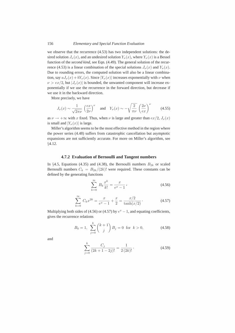
156 Elementary and Special Function Evaluation
we observe that the recurrence (4.53) has two independent solutions: the de-sired solutionJν(x), and an undesired solutionYν(x), whereYν(x) is a Besselfunction of thesecond kind, see Eqn. (4.49). The general solution of the recur-rence (4.53) is a linear combination of the special solutions Jν(x) andYν(x).Due to rounding errors, the computed solution will also be a linear combina-tion, sayaJν(x)+ bYν(x). Since|Yν(x)| increases exponentially withν whenν > ex/2, but |Jν(x)| is bounded, the unwanted component will increase ex-ponentially if we use the recurrence in the forward direction, but decrease ifwe use it in the backward direction.
More precisely, we have
Jν(x) ∼ 1√2πν
(ex
2ν
)ν
and Yν(x) ∼ −√
2
πν
(2ν
ex
)ν
(4.55)
asν → +∞ with x fixed. Thus, whenν is large and greater thanex/2, Jν(x)
is small and|Yν(x)| is large.Miller’s algorithm seems to be the most effective method in the region where
the power series (4.48) suffers from catastrophic cancellation but asymptoticexpansions are not sufficiently accurate. For more on Miller’s algorithm, see§4.12.
4.7.2 Evaluation of Bernoulli and Tangent numbers
In §4.5, Equations (4.35) and (4.38), the Bernoulli numbersB2k or scaledBernoulli numbersCk = B2k/(2k)! were required. These constants can bedefined by the generating functions
∞∑
k=0
Bkxk
k!=
x
ex − 1, (4.56)
∞∑
k=0
Ckx2k =x
ex − 1+
x
2=
x/2
tanh(x/2). (4.57)
Multiplying both sides of (4.56) or (4.57) byex − 1, and equating coefficients,gives the recurrence relations
B0 = 1,
k∑
j=0
(k + 1
j
)Bj = 0 for k > 0, (4.58)
andk∑
j=0
Cj
(2k + 1 − 2j)!=
1
2 (2k)!. (4.59)
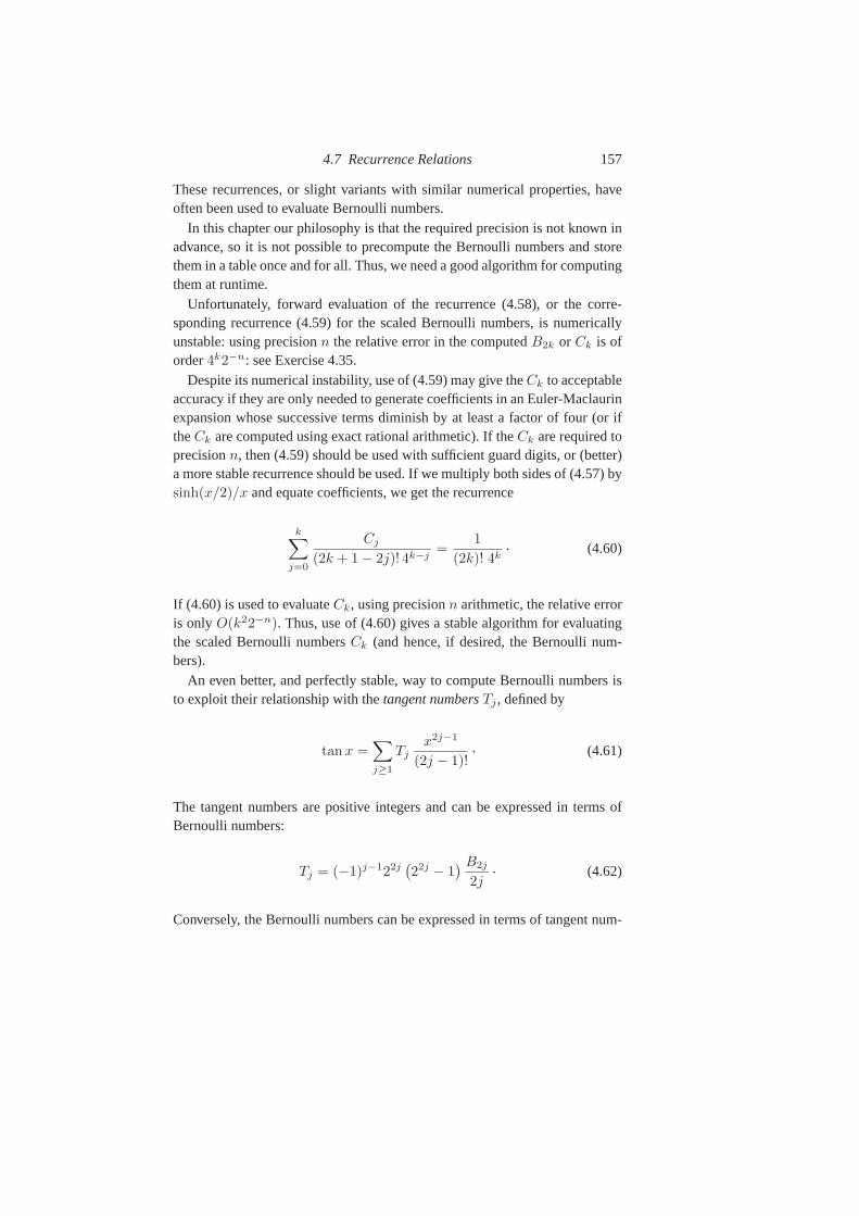
4.7 Recurrence Relations 157
These recurrences, or slight variants with similar numerical properties, haveoften been used to evaluate Bernoulli numbers.
In this chapter our philosophy is that the required precision is not known inadvance, so it is not possible to precompute the Bernoulli numbers and storethem in a table once and for all. Thus, we need a good algorithmfor computingthem at runtime.
Unfortunately, forward evaluation of the recurrence (4.58), or the corre-sponding recurrence (4.59) for the scaled Bernoulli numbers, is numericallyunstable: using precisionn the relative error in the computedB2k or Ck is oforder4k2−n: see Exercise 4.35.
Despite its numerical instability, use of (4.59) may give theCk to acceptableaccuracy if they are only needed to generate coefficients in an Euler-Maclaurinexpansion whose successive terms diminish by at least a factor of four (or iftheCk are computed using exact rational arithmetic). If theCk are required toprecisionn, then (4.59) should be used with sufficient guard digits, or (better)a more stable recurrence should be used. If we multiply both sides of (4.57) bysinh(x/2)/x and equate coefficients, we get the recurrence
k∑
j=0
Cj
(2k + 1 − 2j)! 4k−j=
1
(2k)! 4k. (4.60)
If (4.60) is used to evaluateCk, using precisionn arithmetic, the relative erroris only O(k22−n). Thus, use of (4.60) gives a stable algorithm for evaluatingthe scaled Bernoulli numbersCk (and hence, if desired, the Bernoulli num-bers).
An even better, and perfectly stable, way to compute Bernoulli numbers isto exploit their relationship with thetangent numbersTj , defined by
tan x =∑
j≥1
Tjx2j−1
(2j − 1)!. (4.61)
The tangent numbers are positive integers and can be expressed in terms ofBernoulli numbers:
Tj = (−1)j−122j(22j − 1
) B2j
2j. (4.62)
Conversely, the Bernoulli numbers can be expressed in termsof tangent num-
158 Elementary and Special Function Evaluation
bers:
Bj =
1 if j = 0,
−1/2 if j = 1,
(−1)j/2−1jTj/2/(4j − 2j) if j > 0 is even,
0 otherwise.
Eqn. (4.62) shows that the odd primes in the denominator of the BernoullinumberB2j must be divisors of22j − 1. In fact, this is a consequence ofFermat’s little theorem and the Von Staudt-Clausen theorem, which says thatthe primesp dividing the denominator ofB2j are precisely those for which(p − 1)|2j (see§4.12).
We now derive a recurrence that can be used to compute tangentnumbers,using only integer arithmetic. For brevity writet = tanx andD = d/dx.ThenDt = sec2 x = 1 + t2. It follows thatD(tn) = ntn−1(1 + t2) for alln ∈ N∗.
It is clear thatDnt is a polynomial int, sayPn(t). For example,P0(t) = t,P1(t) = 1+t2, etc.WritePn(t) =
∑j≥0 pn,jt
j . From the recurrencePn(t) =
DPn−1(t), and the formula forD(tn) just noted, we see thatdeg(Pn) = n+1
and ∑
j≥0
pn,jtj =
∑
j≥0
jpn−1,jtj−1(1 + t2),
so
pn,j = (j − 1)pn−1,j−1 + (j + 1)pn−1,j+1 (4.63)
for all n ∈ N∗. Using (4.63) it is straightforward to compute the coefficients ofthe polynomialsP1(t), P2(t), etc.
Algorithm 4.3 TangentNumbersInput: positive integermOutput: Tangent numbersT1, . . . , Tm
T1 ← 1
for k from 2 to m doTk ← (k − 1)Tk−1
for k from 2 to m dofor j from k to m do
Tj ← (j − k)Tj−1 + (j − k + 2)Tj
returnT1, T2, . . . , Tm.
Observe that, sincetan x is an odd function ofx, the polynomialsP2k(t) are
4.7 Recurrence Relations 159
odd, and the polynomialsP2k+1(t) are even. Equivalently,pn,j = 0 if n + j iseven.
We are interested in the tangent numbersTk = P2k−1(0) = p2k−1,0. Us-ing the recurrence (4.63) but avoiding computation of the coefficients thatare known to vanish, we obtain AlgorithmTangentNumbersfor the in-placecomputation of tangent numbers. Note that this algorithm uses only arithmeticon non-negative integers. If implemented with single-precision integers, theremay be problems with overflow as the tangent numbers grow rapidly. If imple-mented using floating-point arithmetic, it is numerically stable because thereis no cancellation. An analogous algorithmSecantNumbersis the topic ofExercise 4.40.
The tangent numbers grow rapidly because the generating functiontan x haspoles atx = ±π/2. Thus, we expectTk to grow roughly like(2k−1)! (2/π)2k.More precisely,
Tk
(2k − 1)!=
22k+1(1 − 2−2k)ζ(2k)
π2k, (4.64)
whereζ(s) is the usual Riemann zeta-function, and
(1 − 2−s)ζ(s) = 1 + 3−s + 5−s + · · ·
is sometimes called theoddzeta-function.The Bernoulli numbers also grow rapidly, but not quite as fast as the tangent
numbers, because the singularities of the generating function (4.56) are fur-ther from the origin (at±2iπ instead of±π/2). It is well-known that the Rie-mann zeta-function for even non-negative integer arguments can be expressedin terms of Bernoulli numbers – the relation is
(−1)k−1 B2k
(2k)!=
2ζ(2k)
(2π)2k. (4.65)
Sinceζ(2k) = 1 + O(4−k) ask → +∞, we see that
|B2k| ∼2 (2k)!
(2π)2k. (4.66)
It is easy to see that (4.64) and (4.65) are equivalent, in view of the rela-tion (4.62).
An asymptotically fast way of computing Bernoulli numbers is the topic ofExercise 4.41. For yet another way of computing Bernoulli numbers, usingvery little space, see§4.10.
160 Elementary and Special Function Evaluation
4.8 Arithmetic-Geometric Mean
The (theoretically) fastest known methods for very large precisionn use thearithmetic-geometric mean (AGM) iteration of Gauss and Legendre. The AGMis another nonlinear recurrence, important enough to treatseparately. Its com-plexity isO(M(n) ln n); the implicit constant here can be quite large, so othermethods are better for smalln.
Given(a0, b0), the AGM iteration is defined by
(aj+1, bj+1) =
(aj + bj
2,√
ajbj
).
For simplicity we only consider real, positive starting values (a0, b0) here(for complex starting values, see§§4.8.5, 4.12). The AGM iteration convergesquadraticallyto a limit which we denote byAGM(a0, b0).
The AGM is useful because:
1. it converges quadratically. Eventually the number of correct digits doublesat each iteration, so onlyO(log n) iterations are required;
2. each iteration takes timeO(M(n)) because the square root can be com-puted in timeO(M(n)) by Newton’s method (see§3.5 and§4.2.3);
3. if we take suitable starting values(a0, b0), the resultAGM(a0, b0) can beused to compute logarithms (directly) and other elementaryfunctions (lessdirectly), as well as constants such asπ andln 2.
4.8.1 Elliptic Integrals
The theory of the AGM iteration is intimately linked to the theory of ellipticintegrals. Thecomplete elliptic integral of the first kindis defined by
K(k) =
∫ π/2
0
dθ√1 − k2 sin2 θ
=
∫ 1
0
dt√(1 − t2)(1 − k2t2)
, (4.67)
and thecomplete elliptic integral of the second kindis
E(k) =
∫ π/2
0
√1 − k2 sin2 θ dθ =
∫ 1
0
√1 − k2t2
1 − t2dt,
wherek ∈ [0, 1] is called themodulusandk′ =√
1 − k2 is thecomplemen-tary modulus. It is traditional (though confusing as the prime does not denotedifferentiation) to writeK ′(k) for K(k′) andE′(k) for E(k′).
4.8 Arithmetic-Geometric Mean 161
The Connection With Elliptic Integrals. Gauss discovered that
1
AGM(1, k)=
2
πK ′(k). (4.68)
This identity can be used to compute the elliptic integralK rapidly via theAGM iteration. We can also use it to compute logarithms. Fromthe defini-tion (4.67), we see thatK(k) has a series expansion that converges for|k| < 1
(in fact K(k) = (π/2)F (1/2, 1/2; 1; k2) is a hypergeometric function). Forsmallk we have
K(k) =π
2
(1 +
k2
4+ O(k4)
). (4.69)
It can also be shown that
K ′(k) =2
πln
(4
k
)K(k) − k2
4+ O(k4). (4.70)
4.8.2 First AGM Algorithm for the Logarithm
From the formulæ (4.68), (4.69) and (4.70), we easily get
π/2
AGM(1, k)= ln
(4
k
)(1 + O(k2)
). (4.71)
Thus, ifx = 4/k is large, we have
ln(x) =π/2
AGM(1, 4/x)
(1 + O
(1
x2
)).
If x ≥ 2n/2, we can computeln(x) to precisionn using the AGM iteration. Ittakes about2 lg(n) iterations to converge ifx ∈ [2n/2, 2n].
Note that we need the constantπ, which could be computed by using ourformula twice with slightly different argumentsx1 andx2, then taking differ-ences to approximate(d ln(x)/dx)/π atx1 (see Exercise 4.44). More efficientis to use theBrent-Salamin(or Gauss-Legendre) algorithm, which is based onthe AGM and the Legendre relation
EK ′ + E′K − KK ′ =π
2. (4.72)
Argument Expansion. If x is not large enough, we can compute
ln(2ℓx) = ℓ ln 2 + lnx
162 Elementary and Special Function Evaluation
by the AGM method (assuming the constantln 2 is known). Alternatively, ifx > 1, we can squarex enough times and compute
ln(x2ℓ
)= 2ℓ ln(x).
This method withx = 2 gives a way of computingln 2, assuming we alreadyknowπ.
The Error Term. TheO(k2) error term in the formula (4.71) is a nuisance.A rigorous bound is
∣∣∣∣π/2
AGM(1, k)− ln
(4
k
)∣∣∣∣ ≤ 4k2(8 − ln k) (4.73)
for all k ∈ (0, 1], and the bound can be sharpened to0.37k2(2.4 − ln(k)) ifk ∈ (0, 0.5].
The errorO(k2| ln k|) makes it difficult to accelerate convergence by usinga larger value ofk (i.e., a value ofx = 4/k smaller than2n/2). There is anexactformula which is much more elegant and avoids this problem. Beforegiving this formula we need to define sometheta functionsand show how theycan be used to parameterise the AGM iteration.
4.8.3 Theta Functions
We need the theta functionsθ2(q), θ3(q) andθ4(q), defined for|q| < 1 by:
θ2(q) =+∞∑
n=−∞q(n+1/2)2 = 2q1/4
+∞∑
n=0
qn(n+1), (4.74)
θ3(q) =+∞∑
n=−∞qn2
= 1 + 2+∞∑
n=1
qn2
, (4.75)
θ4(q) = θ3(−q) = 1 + 2
+∞∑
n=1
(−1)nqn2
. (4.76)
Note that the defining power series are sparse so it is easy to computeθ2(q)
andθ3(q) for smallq. Unfortunately, the rectangular splitting method of§4.4.3does not help to speed up the computation.
The asymptotically fastest methods to compute theta functions use the AGM.However, we do not follow this trail because it would lead us in circles! Wewant to use theta functions to give starting values for the AGM iteration.
4.8 Arithmetic-Geometric Mean 163
Theta Function Identities. There are many classical identities involving thetafunctions. Two that are of interest to us are:
θ23(q) + θ2
4(q)
2= θ2
3(q2) and θ3(q)θ4(q) = θ2
4(q2).
The latter may be written as√
θ23(q)θ
24(q) = θ2
4(q2)
to show the connection with the AGM:
AGM(θ23(q), θ
24(q)) = AGM(θ2
3(q2), θ2
4(q2)) = · · ·
= AGM(θ23(q
2k
), θ24(q
2k
)) = · · · = 1
for any |q| < 1. (The limit is 1 becauseq2k
converges to0, thus bothθ3 andθ4 converge to1.) Apart from scaling, the AGM iteration is parameterised by(θ2
3(q2k
), θ24(q
2k
)) for k = 0, 1, 2, . . .
The Scaling Factor. SinceAGM(θ23(q), θ
24(q)) = 1, andAGM(λa, λb) =
λ · AGM(a, b), scaling givesAGM(1, k′) = 1/θ23(q) if k′ = θ2
4(q)/θ23(q).
Equivalently, sinceθ42 + θ4
4 = θ43 (Jacobi),k = θ2
2(q)/θ23(q). However, we
know (from (4.68) withk → k′) that1/AGM(1, k′) = 2K(k)/π, so
K(k) =π
2θ23(q). (4.77)
Thus, the theta functions are closely related to elliptic integrals. In the literatureq is usually called thenomeassociated with the modulusk.
From q to k and k to q. We saw thatk = θ22(q)/θ2
3(q), which givesk interms ofq. There is also a nice inverse formula which givesq in terms ofk:q = exp(−πK ′(k)/K(k)), or equivalently
ln
(1
q
)=
πK ′(k)
K(k). (4.78)
Sasaki and Kanada’s Formula. Substituting (4.68) and (4.77) withk =
θ22(q)/θ2
3(q) into (4.78) gives Sasaki and Kanada’s elegant formula:
ln
(1
q
)=
π
AGM(θ22(q), θ
23(q))
. (4.79)
This leads to the following algorithm to computelnx.
164 Elementary and Special Function Evaluation
4.8.4 Second AGM Algorithm for the Logarithm
Supposex is large. Letq = 1/x, computeθ2(q4) andθ3(q
4) from their defin-ing series (4.74) and (4.75), then computeAGM(θ2
2(q4), θ2
3(q4)). Sasaki and
Kanada’s formula (withq replaced byq4 to avoid theq1/4 term in the definitionof θ2(q)) gives
ln(x) =π/4
AGM(θ22(q
4), θ23(q
4)).
There is a trade-off between increasingx (by squaring or multiplication by apower of2, see the paragraph on “Argument Expansion” in§4.8.2), and tak-ing longer to computeθ2(q
4) andθ3(q4) from their series. In practice it seems
good to increasex until q = 1/x is small enough thatO(q36) terms are negli-gible. Then we can use
θ2(q4) = 2
(q + q9 + q25 + O(q49)
),
θ3(q4) = 1 + 2
(q4 + q16 + O(q36)
).
We needx ≥ 2n/36 which is much better than the requirementx ≥ 2n/2 forthe first AGM algorithm. We save about four AGM iterations at the cost of afew multiplications.
Implementation Notes. Since
AGM(θ22, θ
23) =
AGM(θ22 + θ2
3, 2θ2θ3)
2,
we can avoid the first square root in the AGM iteration. Also, it only takes twononscalar multiplications to compute2θ2θ3 andθ2
2 + θ23 from θ2 andθ3: see
Exercise 4.45. Another speedup is possible by trading the multiplications forsquares, see§4.12.
Drawbacks of the AGM. The AGM has three drawbacks:
1. the AGM iteration isnotself-correcting, so we have to work with full preci-sion (plus any necessary guard digits) throughout. In contrast, when usingNewton’s method or evaluating power series, many of the computationscan be performed with reduced precision, which saves alog n factor (thisamounts to using anegativenumber of guard digits);
2. the AGM with real arguments givesln(x) directly. To obtainexp(x) weneed to apply Newton’s method (§4.2.5 and Exercise 4.6). To evaluatetrigonometric functions such assin(x), cos(x), arctan(x) we need to workwith complex arguments, which increases the constant hidden in the “O”
4.8 Arithmetic-Geometric Mean 165
time bound. Alternatively, we can use Landen transformations for incom-plete elliptic integrals, but this gives even larger constants;
3. because it converges so fast, it is difficult to speed up theAGM. At best wecan saveO(1) iterations (see however§4.12).
4.8.5 The Complex AGM
In some cases the asymptotically fastest algorithms require the use of complexarithmetic to produce a real result. It would be nice to avoidthis because com-plex arithmetic is significantly slower than real arithmetic. Examples where weseem to need complex arithmetic to get the asymptotically fastest algorithmsare:
1. arctan(x), arcsin(x), arccos(x) via the AGM, using, for example,
arctan(x) = ℑ(ln(1 + ix));
2. tan(x), sin(x), cos(x) using Newton’s method and the above, or
cos(x) + i sin(x) = exp(ix),
where the complex exponential is computed by Newton’s method from thecomplex logarithm (see Eqn. (4.11)).
The theory that we outlined for the AGM iteration and AGM algorithms forln(z) can be extended without problems to complexz /∈ (−∞, 0], providedwe always choose the square root with positive real part.
A complex multiplication takes three real multiplications(using Karatsuba’strick), and a complex squaring takes two real multiplications. We can do evenbetter in the FFT domain, assuming that one multiplication of cost M(n) isequivalent to three Fourier transforms. In this model a squaring costs2M(n)/3.A complex multiplication(a+ib)(c+id) = (ac−bd)+i(ad+bc) requires fourforward and two backward transforms, thus costs2M(n). A complex squaring(a + ib)2 = (a + b)(a − b) + i(2ab) requires two forward and two backwardtransforms, thus costs4M(n)/3. Taking this into account, we get the asymp-totic upper bounds relative to the cost of one multiplication given in Table 4.1(0.666 should be interpreted as∼ 2M(n)/3, and so on). See§4.12 for detailsof the algorithms giving these constants.
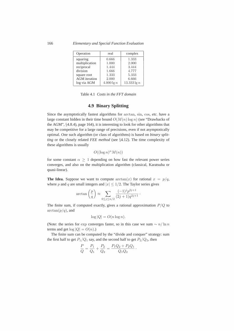
166 Elementary and Special Function Evaluation
Operation real complex
squaring 0.666 1.333multiplication 1.000 2.000reciprocal 1.444 3.444division 1.666 4.777square root 1.333 5.333AGM iteration 2.000 6.666log via AGM 4.000 lg n 13.333 lg n
Table 4.1Costs in the FFT domain
4.9 Binary Splitting
Since the asymptotically fastest algorithms forarctan, sin, cos, etc. have alarge constant hidden in their time boundO(M(n) log n) (see “Drawbacks ofthe AGM”, §4.8.4), page 164), it is interesting to look for other algorithms thatmay be competitive for a large range of precisions, even if not asymptoticallyoptimal. One such algorithm (or class of algorithms) is based onbinary split-ting or the closely relatedFEE method(see§4.12). The time complexity ofthese algorithms is usually
O((log n)αM(n))
for some constantα ≥ 1 depending on how fast the relevant power seriesconverges, and also on the multiplication algorithm (classical, Karatsuba orquasi-linear).
The Idea. Suppose we want to computearctan(x) for rational x = p/q,wherep andq are small integers and|x| ≤ 1/2. The Taylor series gives
arctan
(p
q
)≈
∑
0≤j≤n/2
(−1)jp2j+1
(2j + 1)q2j+1.
The finite sum, if computed exactly, gives a rational approximationP/Q toarctan(p/q), and
log |Q| = O(n log n).
(Note: the series forexp converges faster, so in this case we sum∼ n/ ln n
terms and getlog |Q| = O(n).)The finite sum can be computed by the “divide and conquer” strategy: sum
the first half to getP1/Q1 say, and the second half to getP2/Q2, then
P
Q=
P1
Q1+
P2
Q2=
P1Q2 + P2Q1
Q1Q2
.
4.9 Binary Splitting 167
The rationalsP1/Q1 andP2/Q2 are computed by a recursive application ofthe same method, hence the term “binary splitting”. If used with quadraticmultiplication, this way of computingP/Q does not help; however, fast mul-tiplication speeds up the balanced productsP1Q2, P2Q1, andQ1Q2.
Complexity. The overall time complexity is
O
⌈lg(n)⌉∑
k=1
2k M(2−kn log n)
= O((log n)αM(n)), (4.80)
whereα = 2 in the FFT range; in generalα ≤ 2 (see Exercise 4.47).
We can save a little by working to precisionn rather thann log n at the toplevels; but we still haveα = 2 for quasi-linear multiplication.
In practice the multiplication algorithm would not be fixed but would dependon the size of the integers being multiplied. The complexitywould depend onthe algorithm(s) used at the top levels.
Repeated Application of the Idea. If x ∈ (0, 0.25) and we want to computearctan(x), we can approximatex by a rationalp/q and computearctan(p/q)
as a first approximation toarctan(x), say p/q ≤ x < (p + 1)/q. Now,from (4.17),
tan(arctan(x) − arctan(p/q)) =x − p/q
1 + px/q,
so
arctan(x) = arctan(p/q) + arctan(δ),
where
δ =x − p/q
1 + px/q=
qx − p
q + px.
We can apply the same idea to approximatearctan(δ), until eventually we geta sufficiently accurate approximation toarctan(x). Note that|δ| < |x − p/q|< 1/q, so it is easy to ensure that the process converges.
Complexity of Repeated Application. If we use a sequence of aboutlg n
rationalsp1/q1, p2/q2, . . ., where
qi = 22i
,
then the computation of eacharctan(pi/qi) takes timeO((log n)αM(n)), andthe overall time to computearctan(x) is
O((log n)α+1M(n)).
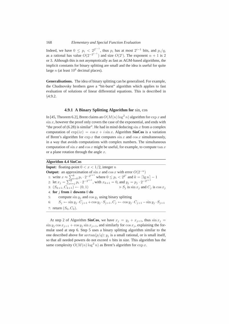
168 Elementary and Special Function Evaluation
Indeed, we have0 ≤ pi < 22i−1
, thuspi has at most2i−1 bits, andpi/qi
as a rational has valueO(2−2i−1
) and sizeO(2i). The exponentα + 1 is 2
or 3. Although this is not asymptotically as fast as AGM-based algorithms, theimplicit constants for binary splitting are small and the idea is useful for quitelargen (at least106 decimal places).
Generalisations. The idea of binary splitting can be generalised. For example,the Chudnovsky brothers gave a “bit-burst” algorithm whichapplies to fastevaluation of solutions of linear differential equations.This is described in§4.9.2.
4.9.1 A Binary Splitting Algorithm for sin, cos
In [45, Theorem 6.2], Brent claims anO(M(n) log2 n) algorithm forexp x andsin x, however the proof only covers the case of the exponential, and ends with“the proof of (6.28) is similar”. He had in mind deducingsinx from a complexcomputation ofexp(ix) = cos x + i sin x. Algorithm SinCos is a variationof Brent’s algorithm forexp x that computessin x andcos x simultaneously,in a way that avoids computations with complex numbers. The simultaneouscomputation ofsin x andcos x might be useful, for example, to computetan x
or a plane rotation through the anglex.
Algorithm 4.4 SinCosInput: floating-point0 < x < 1/2, integernOutput: an approximation ofsin x andcos x with errorO(2−n)
1: write x ≈ ∑ki=0 pi · 2−2i+1
where0 ≤ pi < 22i
andk = ⌈lg n⌉ − 1
2: let xj =∑k
i=j pi · 2−2i+1
, with xk+1 = 0, andyj = pj · 2−2j+1
3: (Sk+1, Ck+1) ← (0, 1) ⊲ Sj is sinxj andCj is cos xj
4: for j from k downto 0 do5: computesin yj andcos yj using binary splitting6: Sj ← sin yj ·Cj+1 +cos yj ·Sj+1, Cj ← cos yj ·Cj+1− sin yj ·Sj+1
7: return(S0, C0).
At step 2 of AlgorithmSinCos, we havexj = yj + xj+1, thussinxj =
sin yj cos xj+1 + cos yj sinxj+1, and similarly forcos xj , explaining the for-mulæ used at step 6. Step 5 uses a binary splitting algorithm similar to theone described above forarctan(p/q): yj is a small rational, or is small itself,so that all needed powers do not exceedn bits in size. This algorithm has thesame complexityO(M(n) log2 n) as Brent’s algorithm forexpx.
4.9 Binary Splitting 169
4.9.2 The Bit-Burst Algorithm
The binary-splitting algorithms described above forarctan x, exp x, sin x relyon a functional equation:tan(x + y) = (tan x + tan y)/(1 − tan x tan y),exp(x + y) = exp(x) exp(y), sin(x + y) = sin x cos y + sin y cos x. Wedescribe here a more general algorithm, known as the “bit-burst” algorithm,which does not require such a functional equation. This algorithm applies toa class of functions known asholonomicfunctions. Other names aredifferen-tiably finiteandD-finite.
A functionf(x) is said to beholonomiciff it satisfies a linear homogeneousdifferential equation with polynomial coefficients inx. Equivalently, the Taylorcoefficientsuk of f satisfy a linear homogeneous recurrence with coefficientspolynomial ink. The set of holonomic functions is closed under the operationsof addition and multiplication, but not necessarily under division. For example,theexp, ln, sin, cos functions are holonomic, buttan is not.
An important subclass of holonomic functions is the hypergeometric func-tions, whose Taylor coefficients satisfy a recurrenceuk+1/uk = R(k), whereR(k) is a rational function ofk (see§4.4). This matches the second defini-tion above, because we can write it asuk+1Q(k) − ukP (k) = 0 if R(k) =
P (k)/Q(k). Holonomic functions are much more general than hypergeometricfunctions (see Exercise 4.48); in particular the ratio of two consecutive termsin a hypergeometric series has sizeO(log k) (as a rational number), but can bemuch larger for holonomic functions.
Theorem 4.9.1 If f is holonomic and has no singularities on a finite, closedinterval [A,B], whereA < 0 < B and f(0) = 0, thenf(x) can be com-puted to an (absolute) accuracy ofn bits, for anyn-bit floating-point numberx ∈ (A,B), in timeO(M(n) log3 n).
NOTES: For a sharper result, see Exercise 4.49. The conditionf(0) = 0 is justa technical condition to simplify the proof of the theorem;f(0) can be anyvalue that can be computed ton bits in timeO(M(n) log3 n).
Proof. Without loss of generality, we assume0 ≤ x < 1 < B; the binaryexpansion ofx can then be writtenx = 0.b1b2 . . . bn. Define r1 = 0.b1,r2 = 0.0b2b3, r3 = 0.000b4b5b6b7 (the same decomposition was already usedin Algorithm SinCos): r1 consists of the first bit of the binary expansion ofx,r2 consists of the next two bits,r3 the next four bits, and so on. We thus havex = r1 + r2 + . . . + rk where2k−1 ≤ n < 2k.
Definexi = r1 + · · · + ri with x0 = 0. The idea of the algorithm is totranslate the Taylor series off from xi to xi+1; sincef is holonomic, this

170 Elementary and Special Function Evaluation
reduces to translating the recurrence on the correspondingcoefficients. Thecondition thatf has no singularity in[0, x] ⊂ [A,B] ensures that the translatedrecurrence is well-defined. We definef0(t) = f(t), f1(t) = f0(r1+t), f2(t) =
f1(r2 + t), . . . , fi(t) = fi−1(ri + t) for i ≤ k. We havefi(t) = f(xi + t),andfk(t) = f(x + t) sincexk = x. Thus we are looking forfk(0) = f(x).
Let f∗i (t) = fi(t) − fi(0) be the non-constant part of the Taylor expan-
sion offi. We havef∗i (ri+1) = fi(ri+1) − fi(0) = fi+1(0) − fi(0) because
fi+1(t) = fi(ri+1 + t). Thus:
f∗0 (r1) + · · · + f∗
k−1(rk) = (f1(0) − f0(0)) + · · · + (fk(0) − fk−1(0))
= fk(0) − f0(0) = f(x) − f(0).
Sincef(0) = 0, this gives:
f(x) =
k−1∑
i=0
f∗i (ri+1).
To conclude the proof, we will show that each termf∗i (ri+1) can be evalu-
ated ton bits in timeO(M(n) log2 n). The rationalri+1 has a numerator of atmost2i bits, and
0 ≤ ri+1 < 21−2i
.
Thus, to evaluatef∗i (ri+1) to n bits,n/2i + O(log n) terms of the Taylor ex-
pansion off∗i (t) are enough. We now use the fact thatf is holonomic. Assume
f satisfies the following homogeneous linear11 differential equation with poly-nomial coefficients:
cm(t)f (m)(t) + · · · + c1(t)f′(t) + c0(t)f(t) = 0.
Substitutingxi + t for t, we obtain a differential equation forfi:
cm(xi + t)f(m)i (t) + · · · + c1(xi + t)f ′
i(t) + c0(xi + t)fi(t) = 0.
From this equation we deduce (see§4.12) a linear recurrence for the Taylorcoefficients offi(t), of the same order as that forf(t). The coefficients in therecurrence forfi(t) haveO(2i) bits, sincexi = r1 + · · · + ri hasO(2i) bits.It follows that theℓ-th Taylor coefficient offi(t) has sizeO(ℓ(2i + log ℓ)).The ℓ log ℓ term comes from the polynomials inℓ in the recurrence. Sinceℓ ≤ n/2i + O(log n), this isO(n log n).
11 If f satisfies a non-homogeneous differential equation, sayE(t, f(t), f ′(t), . . . , f (k)(t)) = b(t), whereb(t) is polynomial int, differentiating it yieldsF (t, f(t), f ′(t), . . . , f (k+1)(t)) = b′(t), andb′(t)E(·) − b(t)F (·) is homogeneous.
4.10 Contour Integration 171
However, we do not want to evaluate theℓ-th Taylor coefficientuℓ of fi(t),but the series
sℓ =
ℓ∑
j=1
ujrji+1 ≈ f∗
i (ri+1).
Noting thatuℓ = (sℓ−sℓ−1)/rℓi+1, and substituting this value in the recurrence
for (uℓ), say of orderd, we obtain a recurrence of orderd + 1 for (sℓ). Puttingthis latter recurrence in matrix formSℓ = MℓSℓ−1, whereSℓ is the vector(sℓ, sℓ−1, . . . , sℓ−d), we obtain
Sℓ = MℓMℓ−1 · · ·Md+1Sd, (4.81)
where the matrix productMℓMℓ−1 · · ·Md+1 can be evaluated in timeO(M(n) log2 n) using binary splitting.
We illustrate Theorem 4.9.1 with the arc-tangent function,which satisfiesthe differential equationf ′(t)(1+ t2) = 1. This equation evaluates atxi + t tof ′
i(t)(1 + (xi + t)2) = 1, wherefi(t) = f(xi + t). This gives the recurrence
(1 + x2i )ℓuℓ + 2xi(ℓ − 1)uℓ−1 + (ℓ − 2)uℓ−2 = 0
for the Taylor coefficientsuℓ of fi. This recurrence translates to
(1 + x2i )ℓvℓ + 2xiri+1(ℓ − 1)vℓ−1 + r2
i+1(ℓ − 2)vℓ−2 = 0
for vℓ = uℓrℓi+1, and to
(1 + x2i )ℓ(sℓ − sℓ−1)
+ 2xiri+1(ℓ − 1)(sℓ−1 − sℓ−2) + r2i+1(ℓ − 2)(sℓ−2 − sℓ−3) = 0
for sℓ =∑ℓ
j=1 vj . This recurrence of order3 can be written in matrix form,and Eqn. (4.81) enables one to efficiently computesℓ ≈ fi(ri + 1) − fi(0)
using multiplication of3 × 3 matrices and fast integer multiplication.
4.10 Contour Integration
In this section we assume that facilities for arbitrary-precision complex arith-metic are available. These can be built on top of an arbitrary-precision realarithmetic package (see Chapters 3 and 5).
Let f(z) be holomorphic in the disc|z| < R, R > 1, and let the powerseries forf be
f(z) =
∞∑
j=0
aj zj . (4.82)
172 Elementary and Special Function Evaluation
From Cauchy’s theorem [122, Ch. 7] we have
aj =1
2πi
∫
C
f(z)
zj+1dz, (4.83)
whereC is the unit circle. The contour integral in (4.83) may be approximatednumerically by sums
Sj,k =1
k
k−1∑
m=0
f(e2πim/k)e−2πijm/k. (4.84)
Let C ′ be a circle with centre at the origin and radiusρ ∈ (1, R). FromCauchy’s theorem, assuming thatj < k, we have (see Exercise 4.50):
Sj,k − aj =1
2πi
∫
C′
f(z)
(zk − 1)zj+1dz = aj+k + aj+2k + · · · , (4.85)
so |Sj,k − aj | = O((R − δ)−(j+k)) ask → ∞, for anyδ > 0. For example,let
f(z) =z
ez − 1+
z
2(4.86)
be the generating function for the scaled Bernoulli numbersas in (4.57), soa2j = Cj = B2j/(2j)! andR = 2π (because of the poles at±2πi). Then
S2j,k − B2j
(2j)!=
B2j+k
(2j + k)!+
B2j+2k
(2j + 2k)!+ · · · , (4.87)
so we can evaluateB2j with relative errorO((2π)−k) by evaluatingf(z) atkpoints on the unit circle.
There is some cancellation when using (4.84) to evaluateS2j,k because theterms in the sum are of order unity but the result is of order(2π)−2j . ThusO(j) guard digits are needed. In the following we assumej = O(n).
If exp(−2πijm/k) is computed efficiently fromexp(−2πi/k) in the obvi-ous way, the time required to evaluateB2, . . . , B2j to precision n isO(jnM(n)), and the space required isO(n). We assume here that we needall Bernoulli numbers up to index2j, but we do not need to store all of themsimultaneously. This is the case if we are using the Bernoulli numbers as coef-ficients in a sum such as (4.38).
The recurrence relation method of§4.7.2 is faster but requires spaceΘ(jn).Thus, the method of contour integration has advantages if space is critical.
For comments on other forms of numerical quadrature, see§4.12.
4.11 Exercises 173
4.11 Exercises
Exercise 4.1 If A(x) =∑
j≥0 ajxj is a formal power series overR with
a0 = 1, show thatln(A(x)) can be computed with errorO(xn) in timeO(M(n)), whereM(n) is the time required to multiply two polynomials ofdegreen − 1. Assume a reasonable smoothness condition on the growth ofM(n) as a function ofn. [Hint: (d/dx) ln(A(x)) = A′(x)/A(x).] Does asimilar result hold forn-bit numbers ifx is replaced by1/2?
Exercise 4.2 (Schonhage[198] and Schost) Assume one wants to compute1/s(x) mod xn, for s(x) a power series. Design an algorithm using an odd-even scheme (§1.3.5), and estimate its complexity in the FFT range.
Exercise 4.3Suppose thatg andh are sufficiently smooth functions satisfyingg(h(x)) = x on some interval. Letyj = h(xj). Show that the iteration
xj+1 = xj +k−1∑
m=1
(y − yj)m g(m)(yj)
m!
is ak-th order iteration that (under suitable conditions) will converge tox =
g(y). [Hint: generalise the argument leading to (4.16).]
Exercise 4.4Design a Horner-like algorithm for evaluating a series∑k
j=0 ajxj
in the forward direction, while deciding dynamically whereto stop. For thestopping criterion, assume that the|aj | are monotonic decreasing and that|x| < 1/2. [Hint: usey = 1/x.]
Exercise 4.5Assume one wantsn bits of exp x for x of order2j , with therepeated use of the doubling formula (§4.3.1), and the naive method to evaluatepower series. What is the best reduced argumentx/2k in terms ofn andj?[Consider both casesj ≥ 0 andj < 0.]
Exercise 4.6Assuming one can compute ann-bit approximation tolnx intime T (n), wheren ≪ M(n) = o(T (n)), show how to compute ann-bitapproximation toexp x in time∼T (n). Assume thatT (n) andM(n) satisfyreasonable smoothness conditions.
Exercise 4.7Care has to be taken to use enough guard digits when computingexp(x) by argument reduction followed by the power series (4.21). If x is oforder unity andk steps of argument reduction are used to computeexp(x) via
exp(x) =(exp(x/2k)
)2k
,
show that aboutk bits of precision will be lost (so it is necessary to use aboutk guard bits).
174 Elementary and Special Function Evaluation
Exercise 4.8Show that the problem analysed in Exercise 4.7 can be avoidedif we work with the function
expm1(x) = exp(x) − 1 =∞∑
j=1
xj
j!
which satisfies the doubling formulaexpm1(2x) = expm1(x)(2+expm1(x)).
Exercise 4.9Forx > −1, prove the reduction formula
log1p(x) = 2 log1p
(x
1 +√
1 + x
)
where the functionlog1p(x) is defined bylog1p(x) = ln(1 + x), as in§4.4.2.Explain why it might be desirable to work withlog1p instead ofln in orderto avoid loss of precision (in the argument reduction, rather than in the recon-struction as in Exercise 4.7). Note however that argument reduction forlog1p
is more expensive than that forexpm1, because of the square root.
Exercise 4.10Give a numerically stable way of computingsinh(x) using oneevaluation ofexpm1(|x|) and a small number of additional operations (com-pare Eqn. (4.20)).
Exercise 4.11 (White)Show thatexp(x) can be computed viasinh(x) usingthe formula
exp(x) = sinh(x) +
√1 + sinh2(x).
Since
sinh(x) =ex − e−x
2=
∑
k≥0
x2k+1
(2k + 1)!,
this saves computing about half the terms in the power seriesfor exp(x) at theexpense of one square root. How would you modify this method to preservenumerical stability for negative argumentsx? Can this idea be used for otherfunctions thanexp(x)?
Exercise 4.12Count precisely the number of nonscalar products necessaryforthe two variants of rectangular series splitting (§4.4.3).
Exercise 4.13A drawback of rectangular series splitting as presented in§4.4.3is that the coefficients (akℓ+m in the classical splitting, orajm+ℓ in the mod-ular splitting) involved in the scalar multiplications might become large. In-deed, they are typically a product of factorials, and thus have sizeO(d log d).Assuming that the ratiosai+1/ai are small rationals, propose an alternate wayof evaluatingP (x).
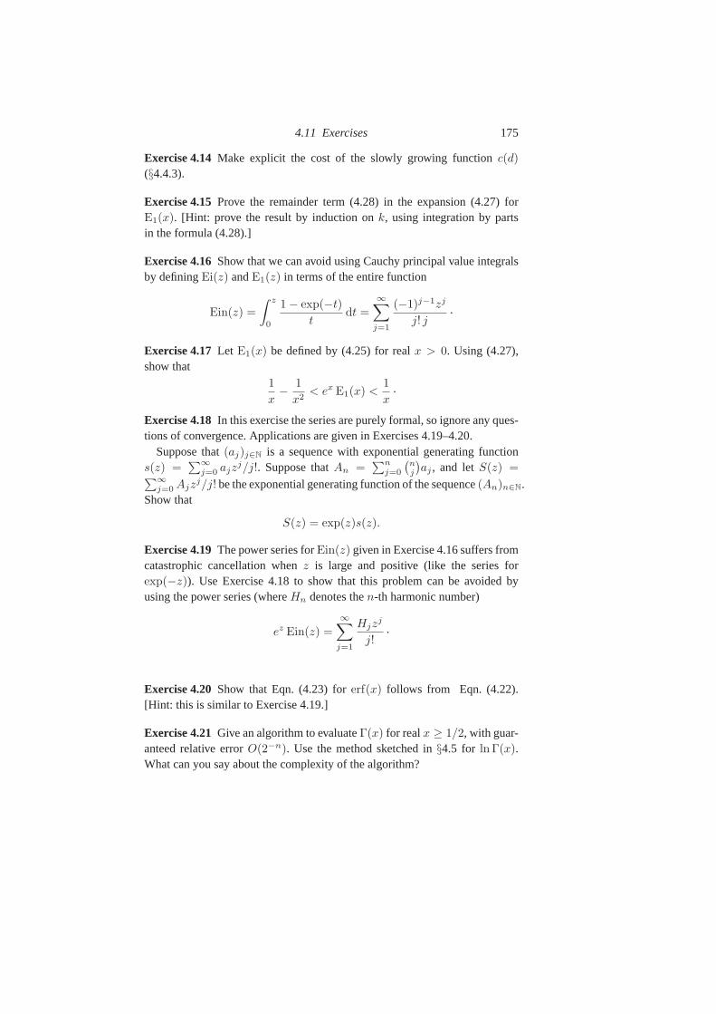
4.11 Exercises 175
Exercise 4.14Make explicit the cost of the slowly growing functionc(d)
(§4.4.3).
Exercise 4.15Prove the remainder term (4.28) in the expansion (4.27) forE1(x). [Hint: prove the result by induction onk, using integration by partsin the formula (4.28).]
Exercise 4.16Show that we can avoid using Cauchy principal value integralsby definingEi(z) andE1(z) in terms of the entire function
Ein(z) =
∫ z
0
1 − exp(−t)
tdt =
∞∑
j=1
(−1)j−1zj
j! j.
Exercise 4.17Let E1(x) be defined by (4.25) for realx > 0. Using (4.27),show that
1
x− 1
x2< ex E1(x) <
1
x.
Exercise 4.18In this exercise the series are purely formal, so ignore any ques-tions of convergence. Applications are given in Exercises 4.19–4.20.
Suppose that(aj)j∈N is a sequence with exponential generating functions(z) =
∑∞j=0 ajz
j/j!. Suppose thatAn =∑n
j=0
(nj
)aj , and letS(z) =∑∞
j=0 Ajzj/j! be the exponential generating function of the sequence(An)n∈N.
Show that
S(z) = exp(z)s(z).
Exercise 4.19The power series forEin(z) given in Exercise 4.16 suffers fromcatastrophic cancellation whenz is large and positive (like the series forexp(−z)). Use Exercise 4.18 to show that this problem can be avoided byusing the power series (whereHn denotes then-th harmonic number)
ez Ein(z) =∞∑
j=1
Hjzj
j!.
Exercise 4.20Show that Eqn. (4.23) forerf(x) follows from Eqn. (4.22).[Hint: this is similar to Exercise 4.19.]
Exercise 4.21Give an algorithm to evaluateΓ(x) for realx ≥ 1/2, with guar-anteed relative errorO(2−n). Use the method sketched in§4.5 for ln Γ(x).What can you say about the complexity of the algorithm?
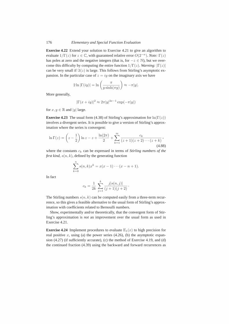
176 Elementary and Special Function Evaluation
Exercise 4.22Extend your solution to Exercise 4.21 to give an algorithm toevaluate1/Γ(z) for z ∈ C, with guaranteed relative errorO(2−n). Note:Γ(z)
has poles at zero and the negative integers (that is, for−z ∈ N), but we over-come this difficulty by computing the entire function1/Γ(z). Warning:|Γ(z)|can be very small ifℑ(z) is large. This follows from Stirling’s asymptotic ex-pansion. In the particular case ofz = iy on the imaginary axis we have
2 ln |Γ(iy)| = ln
(π
y sinh(πy)
)≈ −π|y|.
More generally,
|Γ(x + iy)|2 ≈ 2π|y|2x−1 exp(−π|y|)
for x, y ∈ R and|y| large.
Exercise 4.23The usual form (4.38) of Stirling’s approximation forln(Γ(z))
involves a divergent series. It is possible to give a versionof Stirling’s approx-imation where the series is convergent:
ln Γ(z) =
(z − 1
2
)ln z − z +
ln(2π)
2+
∞∑
k=1
ck
(z + 1)(z + 2) · · · (z + k),
(4.88)where the constantsck can be expressed in terms ofStirling numbers of thefirst kind, s(n, k), defined by the generating function
n∑
k=0
s(n, k)xk = x(x − 1) · · · (x − n + 1).
In fact
ck =1
2k
k∑
j=1
j|s(n, j)|(j + 1)(j + 2)
.
The Stirling numberss(n, k) can be computed easily from a three-term recur-rence, so this gives a feasible alternative to the usual formof Stirling’s approx-imation with coefficients related to Bernoulli numbers.
Show, experimentally and/or theoretically, that the convergent form of Stir-ling’s approximation isnot an improvement over the usual form as used inExercise 4.21.
Exercise 4.24Implement procedures to evaluateE1(x) to high precision forreal positivex, using (a) the power series (4.26), (b) the asymptotic expan-sion (4.27) (if sufficiently accurate), (c) the method of Exercise 4.19, and (d)the continued fraction (4.39) using the backward and forward recurrences as
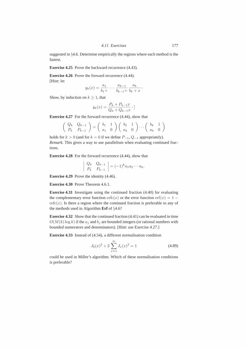
4.11 Exercises 177
suggested in§4.6. Determine empirically the regions where each method isthefastest.
Exercise 4.25Prove the backward recurrence (4.43).
Exercise 4.26Prove the forward recurrence (4.44).[Hint: let
yk(x) =a1
b1+· · · ak−1
bk−1+
ak
bk + x.
Show, by induction onk ≥ 1, that
yk(x) =Pk + Pk−1x
Qk + Qk−1x. ]
Exercise 4.27For the forward recurrence (4.44), show that(
Qk Qk−1
Pk Pk−1
)=
(b1 1
a1 0
) (b2 1
a2 0
)· · ·
(bk 1
ak 0
)
holds fork > 0 (and fork = 0 if we defineP−1, Q−1 appropriately).Remark.This gives a way to use parallelism when evaluating continued frac-tions.
Exercise 4.28For the forward recurrence (4.44), show that∣∣∣∣
Qk Qk−1
Pk Pk−1
∣∣∣∣ = (−1)ka1a2 · · · ak.
Exercise 4.29Prove the identity (4.46).
Exercise 4.30Prove Theorem 4.6.1.
Exercise 4.31Investigate using the continued fraction (4.40) for evaluatingthe complementary error functionerfc(x) or the error functionerf(x) = 1 −erfc(x). Is there a region where the continued fraction is preferable to any ofthe methods used in AlgorithmErf of §4.6?
Exercise 4.32Show that the continued fraction (4.41) can be evaluated in timeO(M(k) log k) if the aj andbj are bounded integers (or rational numbers withbounded numerators and denominators). [Hint: use Exercise4.27.]
Exercise 4.33Instead of (4.54), a different normalisation condition
J0(x)2 + 2∞∑
ν=1
Jν(x)2 = 1 (4.89)
could be used in Miller’s algorithm. Which of these normalisation conditionsis preferable?
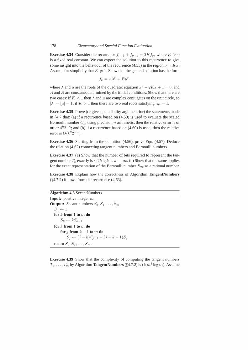
178 Elementary and Special Function Evaluation
Exercise 4.34Consider the recurrencefν−1 + fν+1 = 2Kfν , whereK > 0
is a fixed real constant. We can expect the solution to this recurrence to givesome insight into the behaviour of the recurrence (4.53) in the regionν ≈ Kx.Assume for simplicity thatK 6= 1. Show that the general solution has the form
fν = Aλν + Bµν ,
whereλ andµ are the roots of the quadratic equationx2 − 2Kx + 1 = 0, andA andB are constants determined by the initial conditions. Show that there aretwo cases: ifK < 1 thenλ andµ are complex conjugates on the unit circle, so|λ| = |µ| = 1; if K > 1 then there are two real roots satisfyingλµ = 1.
Exercise 4.35Prove (or give a plausibility argument for) the statements madein §4.7 that: (a) if a recurrence based on (4.59) is used to evaluate the scaledBernoulli numberCk, using precisionn arithmetic, then the relative error is oforder4k2−n; and (b) if a recurrence based on (4.60) is used, then the relativeerror isO(k22−n).
Exercise 4.36Starting from the definition (4.56), prove Eqn. (4.57). Deducethe relation (4.62) connecting tangent numbers and Bernoulli numbers.
Exercise 4.37(a) Show that the number of bits required to represent the tan-gent numberTk exactly is∼2k lg k ask → ∞. (b) Show that the same appliesfor the exact representation of the Bernoulli numberB2k as a rational number.
Exercise 4.38Explain how the correctness of AlgorithmTangentNumbers(§4.7.2) follows from the recurrence (4.63).
Algorithm 4.5 SecantNumbersInput: positive integermOutput: Secant numbersS0, S1, . . . , Sm
S0 ← 1
for k from 1 to m doSk ← kSk−1
for k from 1 to m dofor j from k + 1 to m do
Sj ← (j − k)Sj−1 + (j − k + 1)Sj
returnS0, S1, . . . , Sm.
Exercise 4.39Show that the complexity of computing the tangent numbersT1, . . . , Tm by AlgorithmTangentNumbers(§4.7.2) isO(m3 log m). Assume
4.11 Exercises 179
that the multiplications of tangent numbersTj by small integers take timeO(log Tj). [Hint: use the result of Exercise 4.37.]
Exercise 4.40Verify that Algorithm SecantNumberscomputes in-place theSecant numbersSk, defined by the generating function
∑
k≥0
Skx2k
(2k)!= sec x =
1
cos x,
in much the same way that AlgorithmTangentNumbers (§4.7.2) computesthe Tangent numbers.
Exercise 4.41 (Harvey)The generating function (4.56) for Bernoulli num-bers can be written as
∑
k≥0
Bkxk
k!= 1
/∑
k≥0
xk
(k + 1)!,
and we can use an asymptotically fast algorithm to compute the first n + 1
terms in the reciprocal of the power series. This should be asymptotically fasterthan using the recurrences given in§4.7.2. Give an algorithm using this ideato compute the Bernoulli numbersB0, B1, . . . , Bn in time O(n2(log n)2+ε).Implement your algorithm and see how largen needs to be for it to be fasterthan the algorithms discussed in§4.7.2.
Algorithm 4.6 SeriesExponentialInput: positive integerm and real numbersa1, a2, . . . , am
Output: real numbersb0, b1, . . . , bm such thatb0 + b1x + · · · + bmxm = exp(a1x + · · · + amxm) + O(xm+1)
b0 ← 1
for k from 1 to m dobk ←
(∑kj=1 jajbk−j
) /k
returnb0, b1, . . . , bm.
Exercise 4.42(a) Show that AlgorithmSeriesExponentialcomputesB(x) =
exp(A(x)) up to terms of orderxm+1, whereA(x) = a1x+a2x2+· · ·+amxm
is input data andB(x) = b0 + b1x+ · · ·+ bmxm is the output. [Hint: compareExercise 4.1.]
180 Elementary and Special Function Evaluation
(b) Apply this to give an algorithm to compute the coefficients bk in Stir-ling’s approximation forn! (or Γ(n + 1)):
n! ∼(n
e
) √2πn
∑
k≥0
bk
nk.
[Hint: we know the coefficients in Stirling’s approximation(4.38) for ln Γ(z)
in terms of Bernoulli numbers.](c) Is this likely to be useful for high-precision computation ofΓ(x) for real
positivex?
Exercise 4.43Deduce from Eqn. (4.69) and (4.70) an expansion ofln(4/k)
with error termO(k4 log(4/k)). Use any means to figure out an effectivebound on theO() term. Deduce an algorithm requiringx ≥ 2n/4 only to getnbits of lnx.
Exercise 4.44Show how bothπ andln 2 can be evaluated using Eqn. (4.71).
Exercise 4.45In §4.8.4 we mentioned that2θ2θ3 andθ22 + θ2
3 can be com-puted using two nonscalar multiplications. For example, wecould (A) com-puteu = (θ2 + θ3)
2 andv = θ2θ3; then the desired values are2v andu − 2v.Alternatively, we could (B) computeu andw = (θ2 − θ3)
2; then the desiredvalues are(u ± w)/2. Which method (A) or (B) is preferable?
Exercise 4.46Improve the constants in Table 4.1.
Exercise 4.47Justify Eqn. (4.80) and give an upper bound on the constantα
if the multiplication algorithm satisfiesM(n) = Θ(nc) for somec ∈ (1, 2].
Exercise 4.48 (Salvy)Is the functionexp(x2) + x/(1 − x2) holonomic?
Exercise 4.49 (van der Hoeven, Mezzarobba)Improve to O(M(n) log2 n)
the complexity given in Theorem 4.9.1.
Exercise 4.50If w = e2πi/k, show that
1
zk − 1=
1
k
k−1∑
m=0
wm
z − wm.
Deduce thatSj,k, defined by Eqn. (4.84), satisfies
Sj,k =1
2πi
∫
C′
zk−j−1
zk − 1f(z) dz
for j < k, where the contourC ′ is as in§4.10. Deduce Eqn. (4.85).Remark. Eqn. (4.85) illustrates the phenomenon ofaliasing: observations at
4.12 Notes and References 181
k points can not distinguish between the Fourier coefficientsaj , aj+k, aj+2k,etc.
Exercise 4.51Show that the sumS2j,k of §4.10 can be computed with (essen-tially) only aboutk/4 evaluations off if k is even. Similarly, show that aboutk/2 evaluations off suffice ifk is odd. On the other hand, show that the errorboundO((2π)−k) following Eqn. (4.87) can be improved ifk is odd.
4.12 Notes and References
One of the main references for special functions is the “Handbook of Mathe-matical Functions” by Abramowitz and Stegun [1], which gives many usefulresults but no proofs. A more recent book is that of Nico Temme[215], and acomprehensive reference is Andrewset al. [4]. A large part of the content ofthis chapter comes from [48], and was implemented in the MP package [47].In the context of floating-point computations, the “Handbook of Floating-PointArithmetic” [57] is a useful reference, especially Chapter11.
The SRT algorithm for division is named after Sweeney, Robertson [190]and Tocher [217]. Original papers on Booth recoding, SRT division, etc., arereprinted in the book by Swartzlander [213]. SRT division issimilar to non-restoring division, but uses a lookup table based on the dividend and the divisorto determine each quotient digit. The Intel Pentiumfdiv bug was caused byan incorrectly initialised lookup table.
Basic material on Newton’s method may be found in many references, forexample the books by Brent [41, Ch. 3], Householder [126] or Traub [219].Some details on the use of Newton’s method in modern processors can befound in [128]. The idea of first computingy−1/2, then multiplying byy togety1/2 (§4.2.3) was pushed further by Karp and Markstein [138], who per-form this at the penultimate iteration, and modify the last iteration of Newton’smethod fory−1/2 to directly gety1/2 (see§1.4.5 for an example of the Karp-Markstein trick for division). For more on Newton’s method for power series,we refer to [43, 52, 56, 143, 151, 203].
Some good references on error analysis of floating-point algorithms are thebooks by Higham [121] and Muller [175]. Older references include Wilkin-son’s classics [229, 230].
Regarding doubling versus tripling: in§4.3.4 we assumed that one multi-plication and one squaring were required to apply the tripling formula (4.19).However, one might use the formsinh(3x) = 3 sinh(x) + 4 sinh3(x), whichrequires only one cubing. Assuming a cubing costs 50% more than a squaring
182 Elementary and Special Function Evaluation
— in the FFT range — the ratio would be1.5 log3 2 ≈ 0.946. Thus, if a spe-cialised cubing routine is available, tripling may sometimes be slightly fasterthan doubling.
For an example of a detailed error analysis of an unrestricted algorithm,see [69].
The idea of rectangular series splitting to evaluate a powerseries withO(√
n)
nonscalar multiplications (§4.4.3) was first published in 1973 by Paterson andStockmeyer [183]. It was rediscovered in the context of multiple-precisionevaluation of elementary functions by Smith [205,§8.7] in 1991. Smith gave itthe name “concurrent series”. Smith proposed modular splitting of the series,but classical splitting seems slightly better. Smith noticed that the simultaneoususe of this fast technique and argument reduction yieldsO(n1/3M(n)) algo-rithms. Earlier, in 1960, Estrin [92] had found a similar technique withn/2
nonscalar multiplications, butO(log n) parallel complexity.There are several variants of the Euler-Maclaurin sum formula, with and
without bounds on the remainder. See for example Abramowitzand Stegun [1,Ch. 23], and Apostol [6].
Most of the asymptotic expansions that we have given in§4.5 may be foundin Abramowitz and Stegun [1]. For more background on asymptotic expan-sions of special functions, see for example the books by de Bruijn [84],Olver [181] and Wong [232]. We have omitted mention of many other use-ful asymptotic expansions, for example all but a few of thosefor Bessel func-tions [226, 228].
Most of the continued fractions mentioned in§4.6 may be found in Abram-owitz and Stegun [1]. The classical theory is given in the books byKhinchin [140] and Wall [225]. Continued fractions are usedin the mannerdescribed in§4.6 in arbitrary-precision packages such as MP [47]. A good re-cent reference on various aspects of continued fractions for the evaluation ofspecial functions is theHandbook of Continued Fractions for Special Func-tions [83]. In particular, Chapter 7 of this book contains a discussion of errorbounds. Our Theorem 4.6.1 is a trivial modification of [83, Theorem 7.5.1].The asymptotically fast algorithm suggested in Exercise 4.32 was given bySchonhage [196].
A proof of a generalisation of (4.54) is given in [4,§4.9]. Miller’s algorithmis due to J. C. P. Miller. It is described, for example, in [1,§9.12, §19.28]and [68,§13.14]. An algorithm is given in [102].
A recurrence based on (4.60) was used to evaluate the scaled Bernoulli num-bersCk in the MP package following a suggestion of Christian Reinsch [48,§12]. Previously, the inferior recurrence (4.59) was widelyused, for examplein [141] and in early versions of the MP package [47,§6.11]. The idea of
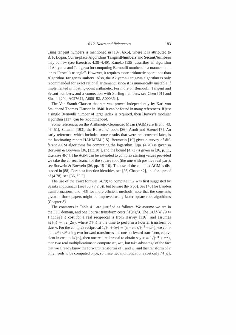
4.12 Notes and References 183
using tangent numbers is mentioned in [107,§6.5], where it is attributed toB. F. Logan. Our in-place AlgorithmsTangentNumbersandSecantNumbersmay be new (see Exercises 4.38–4.40). Kaneko [135] describes an algorithmof Akiyama and Tanigawa for computing Bernoulli numbers in amanner simi-lar to “Pascal’s triangle”. However, it requires more arithmetic operations thanAlgorithm TangentNumbers. Also, the Akiyama-Tanigawa algorithm is onlyrecommended for exact rational arithmetic, since it is numerically unstable ifimplemented in floating-point arithmetic. For more on Bernoulli, Tangent andSecant numbers, and a connection with Stirling numbers, seeChen [61] andSloane [204, A027641, A000182, A000364].
The Von Staudt-Clausen theorem was proved independently byKarl vonStaudt and Thomas Clausen in 1840. It can be found in many references. If justa single Bernoulli number of large index is required, then Harvey’s modularalgorithm [117] can be recommended.
Some references on the Arithmetic-Geometric Mean (AGM) areBrent [43,46, 51], Salamin [193], the Borweins’ book [36], Arndt and Haenel [7]. Anearly reference, which includes some results that were rediscovered later, isthe fascinating report HAKMEM [15]. Bernstein [19] gives a survey of dif-ferent AGM algorithms for computing the logarithm. Eqn. (4.70) is given inBorwein & Borwein [36, (1.3.10)], and the bound (4.73) is given in [36, p. 11,Exercise 4(c)]. The AGM can be extended to complex starting values providedwe take the correct branch of the square root (the one with positive real part):see Borwein & Borwein [36, pp. 15–16]. The use of the complex AGM is dis-cussed in [88]. For theta function identities, see [36, Chapter 2], and for a proofof (4.78), see [36,§2.3].
The use of the exact formula (4.79) to computelnx was first suggested bySasaki and Kanada (see [36, (7.2.5)], but beware the typo). See [46] for Landentransformations, and [43] for more efficient methods; note that the constantsgiven in those papers might be improved using faster square root algorithms(Chapter 3).
The constants in Table 4.1 are justified as follows. We assumewe are inthe FFT domain, and one Fourier transform costsM(n)/3. The13M(n)/9 ≈1.444M(n) cost for a real reciprocal is from Harvey [116], and assumesM(n) ∼ 3T (2n), whereT (n) is the time to perform a Fourier transform ofsizen. For the complex reciprocal1/(v+ iw) = (v− iw)/(v2 +w2), we com-putev2+w2 using two forward transforms and one backward transform, equiv-alent in cost toM(n), then one real reciprocal to obtain sayx = 1/(v2 + w2),then two real multiplications to computevx, wx, but take advantage of the factthat we already know the forward transforms ofv andw, and the transform ofxonly needs to be computed once, so these two multiplicationscost onlyM(n).

184 Elementary and Special Function Evaluation
Thus the total cost is31M(n)/9 ≈ 3.444M(n). The1.666M(n) cost for realdivision is from [125, Remark 6], and assumesM(n) ∼ 3T (2n) as above forthe real reciprocal. For complex division, say(t + iu)/(v + iw), we first com-pute the complex reciprocalx + iy = 1/(v + iw), then perform a complexmultiplication(t + iu)(x + iy), but save the cost of two transforms by observ-ing that the transforms ofx andy are known as a byproduct of the complexreciprocal algorithm. Thus the total cost is(31/9+4/3)M(n) ≈ 4.777M(n).The4M(n)/3 cost for the real square root is from Harvey [116], and assumesM(n) ∼ 3T (2n) as above. The complex square root uses Friedland’s algo-rithm [97]:
√x + iy = w + iy/(2w) wherew =
√(|x| + (x2 + y2)1/2)/2;
as for the complex reciprocal,x2 +y2 costsM(n), then we compute its squareroot in 4M(n)/3, the second square root in4M(n)/3, and the divisiony/w
costs1.666M(n), which gives a total of5.333M(n).The cost of one real AGM iteration is at most the sum of the multiplica-
tion cost and of the square root cost, but since we typically perform severaliterations it is reasonable to assume that the input and output of the iterationincludes the transforms of the operands. The transform ofa + b is obtained bylinearity from the transforms ofa andb, so is essentially free. Thus we saveone transform orM(n)/3 per iteration, giving a cost per iteration of2M(n).(Another way to saveM(n)/3 is to trade the multiplication for a squaring, asexplained in [199,§8.2.5].) The complex AGM is analogous: it costs the sameas a complex multiplication (2M(n)) and a complex square root (5.333M(n)),but we can save two (real) transforms per iteration (2M(n)/3), giving a netcost of6.666M(n). Finally, the logarithm via the AGM costs2 lg(n) + O(1)
AGM iterations.We note that some of the constants in Table 4.1 may not be optimal. For ex-
ample, itmaybe possible to reduce the cost of reciprocal or square root (Har-vey, Sergeev). We leave this as a challenge to the reader (seeExercise 4.46).Note that the constants for operations on power series may differ from thecorresponding constants for operations on integers/reals.
There is some disagreement in the literature about “binary splitting” andthe “FEE method” of E. A. Karatsuba [137].12 We choose the name “binarysplitting” because it is more descriptive, and let the reader call it the “FEEmethod” if he/she prefers. Whatever its name, the idea is quite old, since in1976 Brent [45, Theorem 6.2] gave a binary splitting algorithm to compute
12 It is quite common for the same idea to be discovered independently several times. Forexample, Gauss and Legendre independently discovered the connection between thearithmetic-geometric mean and elliptic integrals; Brent and Salamin independently discoveredan application of this to the computation ofπ, and related algorithms were known to theauthors of [15].
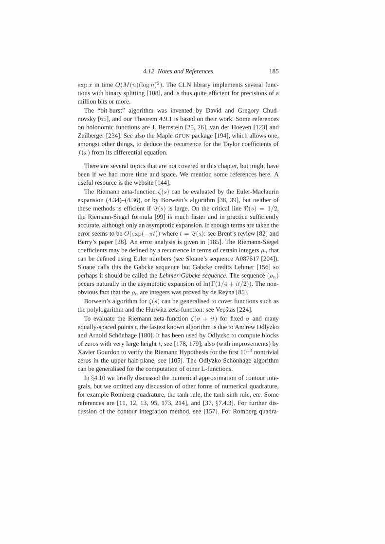
4.12 Notes and References 185
exp x in time O(M(n)(log n)2). The CLN library implements several func-tions with binary splitting [108], and is thus quite efficient for precisions of amillion bits or more.
The “bit-burst” algorithm was invented by David and GregoryChud-novsky [65], and our Theorem 4.9.1 is based on their work. Some referenceson holonomic functions are J. Bernstein [25, 26], van der Hoeven [123] andZeilberger [234]. See also the MapleGFUN package [194], which allows one,amongst other things, to deduce the recurrence for the Taylor coefficients off(x) from its differential equation.
There are several topics that are not covered in this chapter, but might havebeen if we had more time and space. We mention some referenceshere. Auseful resource is the website [144].
The Riemann zeta-functionζ(s) can be evaluated by the Euler-Maclaurinexpansion (4.34)–(4.36), or by Borwein’s algorithm [38, 39], but neither ofthese methods is efficient ifℑ(s) is large. On the critical lineℜ(s) = 1/2,the Riemann-Siegel formula [99] is much faster and in practice sufficientlyaccurate, although only an asymptotic expansion. If enoughterms are taken theerror seems to beO(exp(−πt)) wheret = ℑ(s): see Brent’s review [82] andBerry’s paper [28]. An error analysis is given in [185]. The Riemann-Siegelcoefficients may be defined by a recurrence in terms of certainintegersρn thatcan be defined using Euler numbers (see Sloane’s sequence A087617 [204]).Sloane calls this the Gabcke sequence but Gabcke credits Lehmer [156] soperhaps it should be called theLehmer-Gabcke sequence. The sequence(ρn)
occurs naturally in the asymptotic expansion ofln(Γ(1/4 + it/2)). The non-obvious fact that theρn are integers was proved by de Reyna [85].
Borwein’s algorithm forζ(s) can be generalised to cover functions such asthe polylogarithm and the Hurwitz zeta-function: see Vepstas [224].
To evaluate the Riemann zeta-functionζ(σ + it) for fixed σ and manyequally-spaced pointst, the fastest known algorithm is due to Andrew Odlyzkoand Arnold Schonhage [180]. It has been used by Odlyzko to compute blocksof zeros with very large heightt, see [178, 179]; also (with improvements) byXavier Gourdon to verify the Riemann Hypothesis for the first1013 nontrivialzeros in the upper half-plane, see [105]. The Odlyzko-Schonhage algorithmcan be generalised for the computation of other L-functions.
In §4.10 we briefly discussed the numerical approximation of contour inte-grals, but we omitted any discussion of other forms of numerical quadrature,for example Romberg quadrature, the tanh rule, the tanh-sinh rule,etc.Somereferences are [11, 12, 13, 95, 173, 214], and [37,§7.4.3]. For further dis-cussion of the contour integration method, see [157]. For Romberg quadra-
186 Elementary and Special Function Evaluation
ture (which depends on Richardson extrapolation), see [58,189, 192]. ForClenshaw-Curtis and Gaussian quadrature, see [67, 93, 220]. An example ofthe use of numerical quadrature to evaluateΓ(x) is [32, p. 188]. This is aninteresting alternative to the method based on Stirling’s asymptotic expansion(4.5).
We have not discussed the computation of specific mathematical constantssuch asπ, γ (Euler’s constant),ζ(3), etc. π can be evaluated usingπ =
4arctan(1) and a fastarctan computation (§4.9.2); or by theGauss-Legendrealgorithm (also known as theBrent-Salaminalgorithm), see [43, 46, 193]. Thisasymptotically fast algorithm is based on the arithmetic-geometric mean andLegendre’s relation (4.72). A recent record computation byBellard [16] useda rapidly-converging series for1/π by the Chudnovsky brothers [64], com-bined with binary splitting. Its complexity isO(M(n) log2 n) (theoreticallyworse than Gauss-Legendre’sO(M(n) log n), but with a small constant fac-tor). There are several popular books onπ: we mention Arndt and Haenel [7].A more advanced book is the one by the Borwein brothers [36].
For a clever implementation of binary splitting and its application to the fastcomputation of constants such asπ andζ(3) — and more generally constantsdefined by hypergeometric series — see Cheng, Hanrot, Thome, Zima andZimmermann [62, 63].
The computation ofγ and its continued fraction is of interest because itis not known whetherγ is rational (though this is unlikely). The best algo-rithm for computingγ appears to be the “Bessel function” algorithm of Brentand McMillan [54], as modified by Papanikolaou and later Gourdon [106] toincorporate binary splitting. A very useful source of information on the evalua-tion of constants (includingπ, e, γ, ln 2, ζ(3)) and certain functions (includingΓ(z) andζ(s)) is Gourdon and Sebah’s web site [106].
A nice book on accurate numerical computations for a diverseset of “SIAM100-Digit Challenge” problems is Bornemann, Laurie, Wagonand Waldvo-gel [32]. In particular, Appendix B of this book considers how to solve theproblems to10, 000-decimal digit accuracy (and succeeds in all cases but one).
5
Implementations and Pointers
Here we present a non-exhaustive list of software packages that(in most cases) the authors have tried, together with some otheruseful pointers. Of course, we can not accept any responsibilityfor bugs/errors/omissions in any of the software or documenta-tion mentioned here —caveat emptor!
Websites change. If any of the websites mentioned here disappearin the future, you may be able to find the new site using a searchengine with appropriate keywords.
5.1 Software Tools
5.1.1 CLN
CLN (Class Library for Numbers,http://www.ginac.de/CLN/ ) is alibrary for efficient computations with all kinds of numbersin arbitrary preci-sion. It was written by Bruno Haible, and is currently maintained by RichardKreckel. It is written in C++ and distributed under the GNU General PublicLicense (GPL). CLN provides some elementary and special functions, and fastarithmetic on large numbers, in particular it implements Schonhage-Strassenmultiplication, and the binary splitting algorithm [108].CLN can be config-ured to use GMP low-levelMPN routines, which improves its performance.
5.1.2 GNU MP (GMP)
The GNU MP library is the main reference for arbitrary-precision arithmetic.It has been developed since 1991 by Torbjorn Granlund and several other con-tributors. GNU MP (GMP for short) implements several of the algorithms de-
188 Implementations and Pointers
scribed in this book. In particular, we recommend reading the “Algorithms”chapter of the GMP reference manual [104]. GMP is written in C, is releasedunder the GNU Lesser General Public License (LGPL), and is available fromhttp://gmplib.org .
GMP’s MPZ class implements arbitrary-precision integers (correspondingto Chapter 1), while theMPF class implements arbitrary-precision floating-point numbers (corresponding to Chapter 3).1 The performance of GMP comesmostly from its low-levelMPN class, which is well designed and highly opti-mized in assembly code for many architectures.
As of version 5.0.0,MPZ implements different multiplication algorithms(schoolbook, Karatsuba, Toom-Cook3-way, 4-way, 6-way, 8-way, and FFTusing Schonhage-Strassen’s algorithm); its division routine implements Algo-rithm RecursiveDivRem(§1.4.3) in the middle range, and beyond that New-ton’s method, with complexityO(M(n)), and so does its square root, whichimplements AlgorithmSqrtRem, since it relies on division. The Newton di-vision first precomputes a reciprocal to precisionn/2, and then performs twosteps of Barrett reduction to precisionn/2: this is an integer variant of Algo-rithm Divide. It also implements unbalanced multiplication, with Toom-Cook(3, 2), (4, 3), (5, 3), (4, 2), or (6, 3) [31]. Functionmpn ni invertappr ,which is not in the public interface, implements AlgorithmApproximate-Reciprocal (§3.4.1). GMP 5.0.0 does not implement elementary or specialfunctions (Chapter 4), nor does it provide modular arithmetic with an invariantdivisor in its public interface (Chapter 2). However, it contains a preliminaryinterface for Montgomery’sREDC algorithm.
MPIR is a “fork” of GMP, with a different license, and variousother dif-ferences that make some functions more efficient with GMP, and some withMPIR; also, the difficulty of compiling under Microsoft operating systems mayvary between the forks. Of course, the developers of GMP and MPIR are con-tinually improving their code, so the situation is dynamic.For more on MPIR,seehttp://www.mpir.org/ .
5.1.3 MPFQ
MPFQ is a software library developed by Pierrick Gaudry and EmmanuelThome for manipulation of finite fields. What makes MPFQ different fromother modular arithmetic libraries is that the target finitefield is given atcom-pile time, thus more specific optimizations can be done. The two main targetsof MPFQ are the Galois fieldsF2n andFp with p prime. MPFQ is available
1 However, the authors of GMP recommend using MPFR (see§5.1.4) for new projects.
5.1 Software Tools 189
from http://www.mpfq.org/ , and is distributed under the GNU LesserGeneral Public License (LGPL).
5.1.4 MPFR
MPFR is a multiple-precision binary floating-point library, written in C, basedon the GNU MP library, and distributed under the GNU Lesser General Pub-lic License (LGPL). It extends the main ideas of the IEEE 754 standard toarbitrary-precision arithmetic, by providingcorrect roundingandexceptions.MPFR implements the algorithms of Chapter 3 and most of thoseof Chap-ter 4, including all mathematical functions defined by the ISO C99 standard.These strong semantics are in most cases achieved with no significant slow-down compared to other arbitrary-precision tools. For details of the MPFRlibrary, seehttp://www.mpfr.org and the paper [96].
5.1.5 Other Multiple-Precision Packages
Without attempting to be exhaustive, we briefly mention someof MPFR’s pre-decessors, competitors, and extensions.
1. ARPREC is a package for multiple-precision floating-point arithmetic, writ-ten by David Baileyet al. in C++/Fortran. The distribution includesThe Ex-perimental Mathematician’s Toolkitwhich is an interactive high-precisionarithmetic computing environment. ARPREC is available from http://crd.lbl.gov/ ˜ dhbailey/mpdist/ .
2. MP [47] is a package for multiple-precision floating-point arithmetic and el-ementary and special function evaluation, written in Fortran77. MP permitsany small baseβ (subject to restrictions imposed by the word-size), and im-plements several rounding modes, though correct rounding-to-nearest is notguaranteed in all cases. MP is now obsolete, and we recommendthe use ofa more modern package such as MPFR. However, much of Chapter 4wasinspired by MP, and some of the algorithms implemented in MP are not yetavailable in later packages, so the source code and documentation may beof interest: seehttp://rpbrent.com/pub/pub043.html .
3. MPC (http://www.multiprecision.org/ ) is a C library for arith-metic using complex numbers with arbitrarily high precision and correctrounding, written by Andreas Enge, Philippe Theveny and Paul Zimmer-mann [90]. MPC is built on and follows the same principles as MPFR.
190 Implementations and Pointers
4. MPFI is a package for arbitrary-precision floating-pointinterval arithmetic,based on MPFR. It can be useful to get rigorous error bounds using intervalarithmetic. Seehttp://mpfi.gforge.inria.fr/ , and also§5.3.
5. Several other interesting/useful packages are listed under “Other RelatedFree Software” at the MPFR websitehttp://www.mpfr.org/ .
5.1.6 Computational Algebra Packages
There are several general-purpose computational algebra packages that incor-porate high-precision or arbitrary-precision arithmetic. These include Magma,Mathematica, Maple and Sage. Of these, Sage is free and open-source; theothers are either commercial or semi-commercial and not open-source. Theauthors of this book have often used Magma, Maple and Sage forprototypingand testing algorithms, since it is usually faster to develop an algorithm in ahigh-level language (at least if one is familiar with it) than in a low-level lan-guage like C, where one has to worry about many details. Of course, if speedof execution is a concern, it may be worthwhile to translate the high-level codeinto a low-level language, but the high-level code will be useful for debuggingthe low-level code.
1. Magma (http://magma.maths.usyd.edu.au/magma/ ) was de-veloped and is supported by John Cannon’s group at the University of Syd-ney. Its predecessor wasCayley, a package designed primarily for compu-tational group theory. However, Magma is a general-purposealgebra pack-age with logical syntax and clear semantics. It includes arbitrary-precisionarithmetic based on GMP, MPFR and MPC. Although Magma is not open-source, it has excellent online documentation.
2. Maple(http://www.maplesoft.com ) is a commercial package orig-inally developed at the University of Waterloo, now by Waterloo Maple,Inc. It uses GMP for its integer arithmetic (though not necessarily the latestversion of GMP, so in some cases calling GMP directly may be significantlyfaster). Unlike most of the other software mentioned in thischapter, Mapleuses radix10 for its floating-point arithmetic.
3. Mathematicais a commercial package produced by Stephen Wolfram’scompany Wolfram Research, Inc. In the past, public documentation onthe algorithms used internally by Mathematica was poor. However, thissituation may be improving. Mathematica now appears to use GMP for its
5.2 Mailing Lists 191
basic arithmetic. For information about Mathematica, seehttp://www.wolfram.com/products/mathematica/ .
4. NTL(http://www.shoup.net/ntl/ ) is a C++ library providing datastructures and algorithms for manipulating arbitrary-length integers, as wellas vectors, matrices, and polynomials over the integers andover finite fields.For example, it is very efficient for operations on polynomials over the fi-nite field F2 (that is,GF(2)). NTL was written by and is maintained byVictor Shoup.
5. PARI/GP(http://pari.math.u-bordeaux.fr/ ) is a computer al-gebra system designed for fast computations in number theory, but alsoable to handle matrices, polynomials, power series, algebraic numbersetc.PARI is implemented as a C library, and GP is the scripting language foran interactive shell giving access to the PARI functions. Overall, PARI is asmall and efficient package. It was originally developed in 1987 by Chris-tian Batut, Dominique Bernardi, Henri Cohen and Michel Olivier at Uni-versite Bordeaux I, and is now maintained by Karim Belabas and manyvolunteers.
6. Sage(http://www.sagemath.org/ ) is a free, open-source mathe-matical software system. It combines the power of many existing open-source packages with a common Python-based interface. According to theSage website, its mission is “Creating a viable free open-source alternativeto Magma, Maple, Mathematica and Matlab”. Sage was started by WilliamStein and is developed by a large team of volunteers. It uses MPIR, MPFR,MPC, MPFI, PARI, NTL,etc.Thus, it is a large system, with many capa-bilities, but occupying a lot of space and taking a long time to compile.
5.2 Mailing Lists
5.2.1 The BNIS Mailing List
The BNIS mailing list was created by Dan Bernstein for “Anything of interestto implementors of large-integer arithmetic packages”. Ithas low traffic (a fewmessages per year only). Seehttp://cr.yp.to/lists.html to sub-scribe. An archive of this list is available athttp://www.nabble.com/cr.yp.to---bnis-f846.html .
192 Implementations and Pointers
5.2.2 The GMP Lists
There are four mailing lists associated with GMP:gmp-bugs for bug reports;gmp-announce for important announcements about GMP, in particular newreleases;gmp-discuss for general discussions about GMP;gmp-develfor technical discussions between GMP developers. We recommend subscrip-tion to gmp-announce (very low traffic), togmp-discuss (medium tohigh traffic), and togmp-devel only if you are interested in the internals ofGMP. Information about these lists (including archives andhow to subscribe)is available fromhttp://gmplib.org/mailman/listinfo/ .
5.2.3 The MPFR List
There is only one mailing list for the MPFR library. Seehttp://www.mpfr.org to subscribe or search through the list archives.
5.3 On-line Documents
TheNIST Digital Library of Mathematical Functions(DLMF) is an ambitiousproject to completely rewrite Abramowitz and Stegun’s classic Handbook ofMathematical Functions[1]. It will be published in book form by CambridgeUniversity Press as well as online athttp://dlmf.nist.gov/ . As ofFebruary 2010 the project is incomplete, but still very useful. For example, itprovides an extensive online bibliography with many hyperlinks athttp://dlmf.nist.gov/bib/ .
The Wolfram Functions Sitehttp://functions.wolfram.com/contains a lot of information about mathematical functions(definition, spe-cific values, general characteristics, representations asseries, limits, integrals,continued fractions, differential equations, transformations, and so on).
The Encyclopedia of Special Functions (ESF) is another niceweb site, whoseoriginality is that all formulæ are automatically generated from very few datathat uniquely define the corresponding function in a generalclass [164]. Thisencyclopedia is currently being reimplemented in the Dynamic Dictionary ofMathematical Functions (DDMF); both are available fromhttp://algo.inria.fr/online.html .
A large amount of information about interval arithmetic (introduction, soft-ware, languages, books, courses, applications) can be found on the IntervalComputations pagehttp://www.cs.utep.edu/interval-comp/ .
5.3 On-line Documents 193
Mike Cowlishaw maintains an extensive bibliography of conversion to andfrom decimal arithmetic athttp://speleotrove.com/decimal/ .
Useful if you want to identify an unknown real constant such as1.414213 · · ·is the Inverse Symbolic Calculator(ISC) by Simon Plouffe (building on ear-lier work by the Borwein brothers) athttp://oldweb.cecm.sfu.ca/projects/ISC/ .
Finally, an extremely useful site for all kinds of integer/rational sequences isNeil Sloane’sOnline Encyclopaedia of Integer Sequences(OEIS) athttp://www.research.att.com/ ˜ njas/sequences/ .

Bibliography
[1] Abramowitz, Milton, and Stegun, Irene A. 1973.Handbook of MathematicalFunctions. Dover. [151, 181, 182, 192]
[2] Agrawal, Manindra, Kayal, Neeraj, and Saxena, Nitin. 2004. PRIMES is in P.Annals of Mathematics, 160, 1–13. [45]
[3] Aho, Alfred V., Hopcroft, John E., and Ullman, Jeffrey D. 1974. The Design andAnalysis of Computer Algorithms. Addison-Wesley. [46, 78]
[4] Andrews, George E., Askey, Richard, and Roy, Ranjan. 1999.Special Functions.Cambridge University Press. [181, 182]
[5] ANSI/IEEE. 2008.IEEE Standard for Binary Floating-Point Arithmetic. Revi-sion of IEEE 754-1985, approved on June 12, 2008 by IEEE Standards Board.[123]
[6] Apostol, Tom M. 1999. An elementary view of Euler’s summation formula. TheAmerican Mathematical Monthly, 106(5), 409–418. [182]
[7] Arndt, Jorg, and Haenel, Christoph. 2001.π Unleashed. Springer-Verlag, Berlin.[183, 186]
[8] Bach, Eric. 1990. A note on square roots in finite fields.IEEE Transactions onInformation Theory, 36(6), 1494–1498. [46]
[9] Bach, Eric, and Shallit, Jeffrey O. 1996.Algorithmic Number Theory, Volume 1:Efficient Algorithms. MIT Press. [46]
[10] Bachmann, Paul. 1902.Niedere Zahlentheorie. Vol. 1. Leipzig: Teubner.Reprinted by Chelsea, New York, 1968. [46]
[11] Bailey, David H. 2006. Tanh-sinh high-precision quadrature. Manuscript,3 pages, Jan 2006: LBNL-60519. Available fromhttp://crd.lbl.gov/
˜ dhbailey/dhbpapers/dhb-tanh-sinh.pdf . [185][12] Bailey, David H., and Borwein, Jonathan M. 2009.High-precision nu-
merical integration: progress and challenges. Manuscript, 19 pages, Jul.2009: LBNL-547E. http://crd.lbl.gov/ ˜ dhbailey/dhbpapers/hp-num-int.pdf . [185]
[13] Bailey, David H., Jeyabalan, Karthik, and Li, Xiaoye S. 2005. A comparisonof three high-precision quadrature schemes.Experimental Mathematics, 14(3),317–329. [185]
[14] Barrett, Paul. 1987. Implementing the Rivest Shamir and Adleman public keyencryption algorithm on a standard digital signal processor. Pages 311–323 of:
196 Bibliography
Odlyzko, A. M. (ed),Advances in Cryptology, Proceedings of Crypto’86. Lec-ture Notes in Computer Science, vol. 263. Springer-Verlag. [77]
[15] Beeler, Michael, Gosper, Richard W., and Schroeppel, Rich. 1972. HAKMEM.Memo 239. MIT Artificial Intelligence Laboratory.http://www.inwap.com/pdp10/hbaker/hakmem/hakmem.html . [183, 184]
[16] Bellard, Fabrice. 2009.Pi Computation Record. http://bellard.org/pi/pi2700e9/announce.html . [186]
[17] Bernstein, Daniel J. 1998. Detecting perfect powers in essentiallylinear time.Mathematics of Computation, 67, 1253–1283. [45]
[18] Bernstein, Daniel J. 2002.Pippenger’s exponentiation algorithm. http://cr.yp.to/papers.html . 21 pages. [78]
[19] Bernstein, Daniel J. 2003.Computing logarithm intervals with the arithmetic-geometric-mean iteration. http://cr.yp.to/arith.html . 8 pages.[183]
[20] Bernstein, Daniel J. 2004a.Removing redundancy in high-precision Newtoniteration. http://cr.yp.to/fastnewton.html . 13 pages. [124, 125]
[21] Bernstein, Daniel J. 2004b.Scaled remainder trees. http://cr.yp.to/arith.html . 8 pages. [43]
[22] Bernstein, Daniel J. 2008.Fast multiplication and its applications. http://cr.yp.to/arith.html . 60 pages. [78]
[23] Bernstein, Daniel J., Lenstra, Hendrik W., Jr., and Pila, Jonathan. 2007. Detect-ing perfect powers by factoring into coprimes.Mathematics of Computation,76(257), 385–388. [45]
[24] Bernstein, Daniel J., and Sorenson, Jonathan P. 2007. Modular exponentia-tion via the explicit Chinese remainder theorem.Mathematics of Computation,76(257), 443–454. [77, 79]
[25] Bernstein, Joseph N. 1971. Modules over a ring of differential operators, studyof the fundamental solutions of equations with constant coefficients.FunctionalAnalysis and its Applications, 5(2), Russian original: 1–16, English translation:89–101. [185]
[26] Bernstein, Joseph N. 1972. The analytic continuation of generalized functionswith respect to a parameter.Functional Analysis and its Applications, 6(4), Rus-sian original: 26–40, English translation: 273–285. [185]
[27] Bernstein, Robert. 1986. Multiplication by integer constants.Software, Practiceand Experience, 16(7), 641–652. [14]
[28] Berry, Michael V. 1995. The Riemann-Siegel expansion for thezeta function:high orders and remainders.Proc. Roy. Soc. London, 450, 439–462. [185]
[29] Bertot, Yves, Magaud, Nicolas, and Zimmermann, Paul. 2002. A proof of GMPsquare root.Journal of Automated Reasoning, 29, 225–252. Special Issue onAutomating and Mechanising Mathematics: In honour of N.G. de Bruijn. [45]
[30] Bluestein, Leo I. 1968. A linear filtering approach to the computation of thediscrete Fourier transform.Northeast Electronics Research and EngineeringMeeting Record, 10, 218–219. [78]
[31] Bodrato, Marco, and Zanoni, Alberto. 2007. Integer and polynomial multiplica-tion: towards optimal Toom-Cook matrices. Pages 17–24 of: Brown, C.W. (ed),Proceedings of the 2007 International Symposium on Symbolic and AlgebraicComputation (ISSAC’07). [44, 188]
Bibliography 197
[32] Bornemann, Folkmar, Laurie, Dirk, Wagon, Stan, and Waldvogel, Jorg. 2004.The SIAM 100-Digit Challenge: A Study in High-Accuracy Numerical Comput-ing. SIAM. [186]
[33] Borodin, Allan, and El-Yaniv, Ran. 1998.Online Computation and CompetitiveAnalysis. Cambridge University Press. [44]
[34] Borodin, Allan, and Moenck, Robert. 1974. Fast modular transforms. Journalof Computer and System Sciences, 8(3), 366–386. [79]
[35] Borodin, Allan, and Munro, Ian. 1975.The Computational Complexity of Alge-braic and Numeric Problems. Elsevier Computer Science Library. [78]
[36] Borwein, Jonathan M., and Borwein, Peter B. 1998.Pi and the AGM: A Studyin Analytic Number Theory and Computational Complexity. Wiley. [183, 186]
[37] Borwein, Jonathan M., Borwein, Peter B., and Girgensohn, Roland. 2004. Ex-perimentation in Mathematics: Computational Paths to Discovery. A. K. Peters.[185]
[38] Borwein, Jonathan M., Bradley, David M., and Crandall, RichardE. 2000. Com-putational strategies for the Riemann zeta function.Journal of Computationaland Applied Mathematics, 121, 247–296. [185]
[39] Borwein, Peter B. 2000.An efficient algorithm for the Riemann zeta function.in Constructive, Experimental, and Nonlinear Analysis (Limoges, 1999), CMSConf. Proc. 27, Amer. Math. Soc. [185]
[40] Bostan, Alin, Lecerf, Gregoire, and Schost,Eric. 2003. Tellegen’s principle intopractice. Pages 37–44 of: Sendra, J. R. (ed),Proceedings of the 2003 Interna-tional Symposium on Symbolic and Algebraic Computation (ISSAC’03). [124]
[41] Brent, Richard P. 1973a.Algorithms for Minimization without Derivatives.Prentice-Hall. Reprinted by Dover, 2002.http://rpbrent.com/pub/pub011.html . [181]
[42] Brent, Richard P. 1973b. On the precision attainable with various floating-pointnumber systems.IEEE Transactions on Computers, C-22, 601–607.http://rpbrent.com/pub/pub017.html . [120, 123]
[43] Brent, Richard P. 1975. Multiple-precision zero-finding methods and the com-plexity of elementary function evaluation. Pages 151–176 of: Traub, J.F. (ed),Analytic Computational Complexity. New York: Academic Press.http://rpbrent.com/pub/pub028.html . [181, 183, 186]
[44] Brent, Richard P. 1976a. Analysis of the binary Euclidean algorithm. Pages321–355 of: Traub, J. F. (ed),New Directions and Recent Results in Algorithmsand Complexity. Academic Press, New York.http://rpbrent.com/pub/pub037.html . Errata: see the online version. [45]
[45] Brent, Richard P. 1976b. The complexity of multiple-precision arithmetic.Pages 126–165 of: Anderssen, R. S., and Brent, R. P. (eds),The Complexityof Computational Problem Solving. University of Queensland Press.http://rpbrent.com/pub/pub032.html . [168, 184]
[46] Brent, Richard P. 1976c. Fast multiple-precision evaluation of elementary func-tions. Journal of the ACM, 23(2), 242–251.http://rpbrent.com/pub/pub034.html . [183, 186]
[47] Brent, Richard P. 1978. Algorithm 524: MP, a Fortran multiple-precisionarithmetic package.ACM Transactions on Mathematical Software, 4, 71–81.http://rpbrent.com/pub/pub043.html . [181, 182, 189]
198 Bibliography
[48] Brent, Richard P. 1980. Unrestricted algorithms for elementary and special func-tions. Pages 613–619 of: Lavington, S. H. (ed),Information Processing, vol. 80.http://rpbrent.com/pub/pub052.html . [123, 181, 182]
[49] Brent, Richard P. 1982. An idealist’s view of semantics for integer and realtypes. Australian Computer Science Communications, 4, 130–140.http://rpbrent.com/pub/pub069.html . [123]
[50] Brent, Richard P. 2000. Twenty years’ analysis of the binary Euclidean algo-rithm. Pages 41–53 of: Davies, J., Roscoe, A. W., and Woodcock, J. (eds),Millennial Perspectives in Computer Science. Palgrave, New York.http://rpbrent.com/pub/pub183.html . [45]
[51] Brent, Richard P. 2006.Fast algorithms for high-precision computation of el-ementary functions. Invited talk presented at the Real Numbers and Computa-tion Conference (RNC7), Nancy, France, July 2006. Available fromhttp://rpbrent.com/talks.html . [183]
[52] Brent, Richard P., and Kung, Hsiang T. 1978. Fast algorithms for manipulat-ing formal power series.Journal of the ACM, 25(2), 581–595. http://rpbrent.com/pub/pub045.html . [181]
[53] Brent, Richard P., and Kung, Hsiang T. 1983. Systolic VLSI arrays for linear-time GCD computation. Pages 145–154 of: Anceau, F., and Aas, E. J. (eds),VLSI83. North Holland, Amsterdam.http://rpbrent.com/pub/pub082.html . [46]
[54] Brent, Richard P., and McMillan, Edwin M. 1980. Some new algorithms forhigh-precision computation of Euler’s constant.Mathematics of Computation,34(149), 305–312.http://rpbrent.com/pub/pub049.html . [186]
[55] Brent, Richard P., Percival, Colin, and Zimmermann, Paul. 2007. Error boundson complex floating-point multiplication.Mathematics of Computation, 76(259),1469–1481.http://rpbrent.com/pub/pub221.html . [124]
[56] Brent, Richard P., and Traub, Joseph F. 1980. On the complexityof compositionand generalized composition of power series.SIAM J. on Computing, 9, 54–66.http://rpbrent.com/pub/pub050.html . [181]
[57] Brisebarre, Nicolas, de Dinechin, Florent, Jeannerod, Claude-Pierre, Lefevre,Vincent, Melquiond, Guillaume, Muller, Jean-Michel, Revol, Nathalie, Stehle,Damien, and Torres, Serge. 2009.Handbook of Floating-Point Arithmetic.Birkhauser. 572 pages. [181]
[58] Bulirsch, Roland, and Stoer, Josef. 1967. Handbook Series Numerical Integra-tion. Numerical quadrature by extrapolation.Numerische Mathematik, 9, 271–278. [186]
[59] Burgisser, Peter, Clausen, Michael, and Shokrollahi, Mohammad A. 1997. Al-gebraic Complexity Theory. Grundlehren der mathematischen Wissenschaften315. Springer. [41, 125]
[60] Burnikel, Christoph, and Ziegler, Joachim. 1998.Fast Recursive Division. Re-search Report MPI-I-98-1-022. MPI Saarbrucken. [45]
[61] Chen, Kwang-Wu. 2001. Algorithms for Bernoulli numbers and Euler numbers.Journal of Integer Sequences, 4. Article 01.1.6, 7 pp. [183]
[62] Cheng, Howard, Hanrot, Guillaume, Thome, Emmanuel, Zima, Eugene, and
Bibliography 199
Zimmermann, Paul. 2007a. Time- and space-efficient evaluation of some hy-pergeometric constants. Pages 85–91 of: Brown, C. W. (ed),Proceedings of the2007 International Symposium on Symbolic(ISSAC’2007). ACM. [186]
[63] Cheng, Howard, Hanrot, Guillaume, Thome, Emmanuel, Zima, Eugene, andZimmermann, Paul. 2007b.Time- and space-efficient evaluation of some hyper-geometric constants. Research Report 6105. INRIA, Jan. 2007, 20 pp.http://hal.inria.fr/inria-00126428 . [186]
[64] Chudnovsky, David V., and Chudnovsky, Gregory G. 1988. Approximations andcomplex multiplication according to Ramanujan. Pages 375–472 of: Andrews,G. E., Berndt, B. C., and Rankin, R. A. (eds),Ramanujan Revisited: Proceedingsof the Centenary Conference. Academic Press, Boston. [186]
[65] Chudnovsky, David V., and Chudnovsky, Gregory V. 1990. Computer algebrain the service of mathematical physics and number theory. Pages 109–232 of:Computers in Mathematics (Stanford, CA, 1986). Lecture Notes in Pure andApplied Mathematics, vol. 125. New York: Dekker. [185]
[66] Chung, Jaewook, and Hasan, M. Anwar. 2007. Asymmetric squaring formulae.Pages 113–122 of: Kornerup, P., and Muller, J.-M. (eds),Proceedings of the18th IEEE Symposium on Computer Arithmetic (ARITH-18). IEEE ComputerSociety. [45]
[67] Clenshaw, Charles W., and Curtis, Alan R. 1960. A method for numerical inte-gration on an automatic computer.Numerische Mathematik, 2, 197–205. [186]
[68] Clenshaw, Charles W., Goodwin, Charles E. T., Martin, David W.,Miller, Geof-frey F., Olver, Frank W. J., and Wilkinson, James H. 1961.Modern ComputingMethods. second edn. Notes on Applied Science, No. 16. HMSO. [182]
[69] Clenshaw, Charles W., and Olver, Frank W. J. 1980. An unrestricted algorithmfor the exponential function.SIAM Journal on Numerical Analysis, 17, 310–331.[123, 182]
[70] Clenshaw, Charles W., and Olver, Frank W. J. 1984. Beyond floating point.Journal of the ACM, 31(2), 319–328. [123]
[71] Clinger, William D. 1990. How to read floating point numbers accurately. Pages92–101 of:Proceedings of the ACM SIGPLAN’90 Conference on ProgrammingLanguage Design and Implementation. [125]
[72] Cody, William J., Coonen, Jerome T., Gay, David M., Hanson, Kenton, Hough,David, Kahan, William, Karpinski, Richard, Palmer, John, Ris, FredericN., andStevenson, David. 1984. A proposed radix- and word-length-independent stan-dard for floating-point arithmetic.IEEE Micro, 86–100. [123]
[73] Cohen, Henri. 1993.A Course in Computational Algebraic Number Theory.Graduate Texts in Mathematics 138. Springer-Verlag. 534 pages. [45,79]
[74] Collins, George E., and Krandick, Werner. 2000. Multiprecision floating pointaddition. Pages 71–77 of: Traverso, C. (ed),Proceedings of the 2000 Interna-tional Symposium on Symbolic and Algebraic Computation (ISSAC’00). ACMPress. [123]
[75] Commerce, U.S. Department Of. 2000.Digital Signature Standard (DSS). Tech.rept. FIPS PUB 186-2. National Institute of Standards and Technology.76 pages.[78]
[76] Cook, Stephen A. 1966.On the Minimum Computation Time of Functions. Ph.D.
200 Bibliography
thesis, Harvard University. Chapter 3 available fromhttp://cr.yp.to/bib/1966/cook.html . [44]
[77] Cornea, Marius, Anderson, Cristina, Harrison, John, Tang, Ping Tak Peter,Schneider, Eric, and Tsen, Charles. 2007. A software implementation of theIEEE 754R decimal floating-point arithmetic using the binary encoding format.Pages 29–37 of:Proceedings of the 18th IEEE Symposium on Computer Arith-metic (ARITH-18). [125]
[78] Cornea-Hasegan, Marius A., Golliver, Roger A., and Markstein, Peter. 1999.Correctness proofs outline for Newton-Raphson based floating-pointdivide andsquare root algorithms. Pages 96–105 of: Koren, I., and Kornerup, P. (eds),Proceedings of the 14th IEEE Symposium on Computer Arithmetic (ARITH-14).[125]
[79] Crandall, Richard E. 1994.Projects in Scientific Computation. TELOS, TheElectronic Library of Science, Santa Clara, California. [124]
[80] Crandall, Richard E. 1996.Topics in Advanced Scientific Computation. TELOS,The Electronic Library of Science, Santa Clara, California. [101, 124]
[81] Crandall, Richard E., and Pomerance, Carl. 2005.Prime Numbers: A Computa-tional Perspective. second edn. Springer-Verlag. [44]
[82] Crary, Fred D., and Rosser, John B. 1977. High precision coefficients relatedto the zeta function.Reviewed in Mathematics of Computation, 31, 803–804.Review available fromhttp://rpbrent.com/review01.html . [185]
[83] Cuyt, Annie, Petersen, Vigdis B., Verdonk, Brigitte, Waadeland, Haakon, andJones, William B. (with contributions by Franky Backeljauw and CatherineBonan-Hamada). 2008.Handbook of Continued Fractions for Special Func-tions. Springer. xvi+431 pages. [182]
[84] de Bruijn, Nicolaas G. 1970 (reprinted by Dover, New York 1981). AsymptoticMethods in Analysis. third edn. North-Holland. [182]
[85] de Reyna, Juan Arias. 2005. Dynamical zeta functions and Kummer congru-ences.Acta Arithmetica, 119(1), 39–52. [185]
[86] Dimitrov, Vassil S., Jullien, Graham A., and Miller, William C. 1998. Analgo-rithm for modular exponentiation.Information Processing Letters, 66, 155–159.[78]
[87] Dixon, Brandon, and Lenstra, Arjen K. 1993. Massively parallel elliptic curvefactoring. Pages 183–193 of:Proceedings of Eurocrypt’92. Lecture Notes inComputer Science, vol. 658. Springer-Verlag. [44]
[88] Dupont, Regis. 2010. Fast evaluation of modular functions using Newton itera-tions and the AGM.Mathematics of Computation. In press, 2010. [183]
[89] Eikenberry, Shawna M., and Sorenson, Jonathan P. 1998. Efficient algorithmsfor computing the Jacobi symbol.Journal of Symbolic Computation, 26(4), 509–523. [46]
[90] Enge, Andreas, Theveny, Philippe, and Zimmermann, Paul. 2009.MPC — Alibrary for multiprecision complex arithmetic with exact rounding. 0.8.1 edn.INRIA. http://mpc.multiprecision.org/ . [189]
[91] Ercegovac, Milos D., and Muller, Jean-Michel. 2007. Complex square root withoperand prescaling.The Journal of VLSI Signal Processing, 49(1), 19–30. [126]
Bibliography 201
[92] Estrin, Gerald. 1960. Organization of computer systems – the fixedplus variablestructure computer. Pages 33–40 of:Proceedings of the Western Joint ComputerConference. [182]
[93] Fejer, Leopold. 1933. On the infinite sequences arising in the theories of har-monic analysis, of interpolation, and of mechanical quadratures.Bulletin of theAmerican Mathematical Society, 39, 521–534. [186]
[94] Forsythe, George E. 1970. Pitfalls in computation, or why a math book isn’tenough.American Mathematical Monthly, 77, 931–956. [140]
[95] Fousse, Laurent. 2006.Integration Numerique avec Erreur Bornee en PrecisionArbitraire. Ph.D. thesis, University Henri Poincare Nancy 1. [185]
[96] Fousse, Laurent, Hanrot, Guillaume, Lefevre, Vincent, Pelissier, Patrick, andZimmermann, Paul. 2007. MPFR: A multiple-precision binary floating-pointlibrary with correct rounding.ACM Transactions on Mathematical Software,33(2), 13:1–13:15. [189]
[97] Friedland, Paul. 1967. Algorithm 312: Absolute value and square root of a com-plex number.Communications of the ACM, 10(10), 665. [184]
[98] Furer, Martin. 2007. Faster integer multiplication. Pages 57–66 of: Johnson,D. S., and Feige, U. (eds),Proceedings of the 39th Annual ACM Symposium onTheory of Computing (STOC), San Diego, California, USA. ACM. [78]
[99] Gabcke, Wolfgang. 1979.Neue Herleitung und explizite Restabschatzung derRiemann-Siegel-Formel. Ph.D. thesis, Georg-August-Universitat, Gottingen.Spanish translation available from Juan Arias de Reyna. [185]
[100] Gathen, Joachim von zur, and Gerhard, Jurgen. 1999. Modern ComputerAlgebra. Cambridge University Press, Cambridge.http://www-math.uni-paderborn.de/mca . [77]
[101] Gauss, Carl F. 1889.Untersuchungenuber Hohere Arithmetik. Springer, Berlin.Reprinted by the American Mathematical Society, 2006. [46]
[102] Gautschi, Walter. 1964. Algorithm 236: Bessel functions of the first kind. Com-munications of the ACM, 7, 479–480. [182]
[103] Gay, David M. 1990. Correctly rounded binary-decimal and decimal-binaryconversions. Numerical Analysis Manuscript 90-10. AT&T Bell Laboratories.[125]
[104] GMP. 2010.GNU MP: The GNU Multiple Precision Arithmetic Library. 5.0.0edn.http://gmplib.org/ . [188]
[105] Gourdon, Xavier. 2004.The1013 first zeros of the Riemann zeta function, andzeros computation at very large height. http://numbers.computation.free.fr/Constants/Miscellaneous/zetazeros1e13-1e24.pdf . [185]
[106] Gourdon, Xavier, and Sebah, Pascal. 2010.Numbers, constants and computa-tion. http://numbers.computation.free.fr/ . [186]
[107] Graham, Ronald L., Knuth, Donald E., and Patashnik, Oren. 1994. ConcreteMathematics. third edn. Addison-Wesley. [183]
[108] Haible, Bruno, and Papanikolaou, Thomas. 1998. Fast multiprecision evaluationof series of rational numbers. Pages 338–350 of: Buhler, J. P. (ed), Proceedingsof the 3rd Algorithmic Number Theory Symposium (ANTS-III). Lecture Notes inComputer Science, vol. 1423. Springer-Verlag. [185, 187]
202 Bibliography
[109] Halfhill, Tom R. 1995. The truth behind the Pentium bug.Byte. March 1995.Available from http://www2.informatik.uni-jena.de/ ˜ nez/rechnerarithmetik_5/fdiv_bug/byte_art1.htm . [130]
[110] Hankerson, Darrel, Menezes, Alfred, and Vanstone, Scott. 2004. Guide to El-liptic Curve Cryptography. Springer-Verlag. http://www.cacr.math.uwaterloo.ca/ecc/ . [78]
[111] Hanrot, Guillaume, Quercia, Michel, and Zimmermann, Paul. 2004. The mid-dle product algorithm, I. Speeding up the division and square root of power se-ries.Applicable Algebra in Engineering, Communication and Computing, 14(6),415–438. [124]
[112] Hanrot, Guillaume, and Zimmermann, Paul. 2004. A long note on Mulders’short product.Journal of Symbolic Computation, 37, 391–401. [45]
[113] Hars, Laszlo. 2004. Long modular multiplication for cryptographic applica-tions. Pages 44–61 of:CHES’04. Lecture Notes in Computer Science, vol.3156. Springer-Verlag. [77]
[114] Harvey, David. 2009a. Faster polynomial multiplication via multipointKro-necker substitution.J. of Symbolic Computation, 44, 1502–1510. [39, 44]
[115] Harvey, David. 2009b.The Karatsuba middle product for integers. http://cims.nyu.edu/ ˜ harvey/mulmid/ . Preprint. [124]
[116] Harvey, David. 2010a. Faster algorithms for the square root and reciprocal ofpower series. Mathematics of Computation. In press, 2010. Available fromhttp://arxiv.org/abs/0910.1926 . [125, 183, 184]
[117] Harvey, David. 2010b. A multimodular algorithm for computing Bernoulli num-bers. Mathematics of Computation. In press, 2010. Available fromhttp://arxiv.org/abs/0807.1347v2 . [183]
[118] Hasenplaugh, William, Gaubatz, Gunnar, and Gopal, Vinodh. 2007. Fast modu-lar reduction. Pages 225–229 of:Proceedings of the 18th IEEE Symposium onComputer Arithmetic (ARITH-18). Montpellier, France: IEEE Computer SocietyPress. [77]
[119] Hastad, Johan. 1990. Tensor rank is NP-complete.Journal of Algorithms, 11(4),644–654. [41]
[120] Hennessy, John L., Patterson, David A., and Goldberg, David. 1990. ComputerArchitecture: A Quantitative Approach. Morgan Kaufmann. [123]
[121] Higham, Nicholas J. 2002.Accuracy and Stability of Numerical Algorithms.second edn. SIAM. [123, 181]
[122] Hille, Einar. 1959.Analytic Function Theory. Vol. 1. Blaisdell, New York. [172][123] Hoeven, Joris van der. 1999. Fast evaluation of holonomic functions.Theoretical
Computer Science, 210, 199–215. [185][124] Hoeven, Joris van der. 2002. Relax, but don’t be too lazy.Journal of Sym-
bolic Computation, 34(6), 479–542. Available fromhttp://www.math.u-psud.fr/ ˜ vdhoeven . [44, 76]
[125] Hoeven, Joris van der. 2006.Newton’s method and FFT trading. Tech.rept. 2006-17. University Paris-Sud.http://www.texmacs.org/joris/fnewton/fnewton-abs.html . [125, 184]
[126] Householder, Alston S. 1970.The Numerical Treatment of a Single NonlinearEquation. McGraw-Hill, New York. [181]
Bibliography 203
[127] Hull, Thomas E. 1982. The use of controlled precision. Pages 71–84 of: Reid,J. K. (ed),The Relationship Between Numerical Computation and ProgrammingLanguages. North Holland. [123]
[128] Intel. 2003.Division, square root and remainder algorithms for the Intel(R) Ita-nium(TM) architecture. Application Note, available fromftp://download.intel.com/software/opensource/divsqrt.pdf , 120 pages. [181]
[129] Iordache, Cristina, and Matula, David W. 1999. On infinitely precise roundingfor division, square root, reciprocal and square root reciprocal.Pages 233–240of: Proceedings of the 14th IEEE Symposium on Computer Arithmetic (ARITH-14). IEEE Computer Society. [124]
[130] Jebelean, Tudor. 1993. An algorithm for exact division.Journal of SymbolicComputation, 15, 169–180. [45]
[131] Jebelean, Tudor. 1995. A double-digit Lehmer-Euclid algorithmfor finding theGCD of long integers.Journal of Symbolic Computation, 19, 145–157. [46]
[132] Jebelean, Tudor. 1997. Practical integer division with Karatsuba complexity.Pages 339–341 of: Kuchlin, W. W. (ed),Proceedings of International Symposiumon Symbolic and Algebraic Computation (ISSAC’97). [45]
[133] Kahan, William M. 2002. Idempotent binary→ decimal → binaryconversion. http://www.cs.berkeley.edu/ ˜ wkahan/Math128/BinDecBin.pdf . 1 page. [125]
[134] Kaihara, Marcelo E., and Takagi, Naofumi. 2008. Bipartite modular multiplica-tion method.IEEE Transactions on Computers, 57(2), 157–164. [78]
[135] Kaneko, Masanobu. 2000. The Akiyama-Tanigawa algorithm for Bernoullinumbers.Journal of Integer Sequences, 3. Article 00.2.9, 6 pages. [183]
[136] Karatsuba, Anatolii A., and Ofman, Yuri. 1962. Multiplication of multi-digitnumbers on automata (in Russian).Doklady Akad. Nauk SSSR, 145(2), 293–294. Translation inSoviet Physics-Doklady7 (1963), 595–596. [44]
[137] Karatsuba, Ekatherina A. 1999. Fast evaluation of hypergeometric functionsby FEE. Pages 303–314 of: Papamichael, N., Ruscheweyh, St., andSaff, E. B.(eds),Proceedings of Computational Methods and Function Theory (CMFT’97).World Scientific Publishing. [184]
[138] Karp, Alan H., and Markstein, Peter. 1997. High-precision division and squareroot. ACM Trans. on Mathematical Software, 23(4), 561–589. [45, 125, 181]
[139] Khachatrian, Gurgen H., Kuregian, Melsik K., Ispiryan, Karen R., and Massey,James L. 2001. Fast multiplication of integers for public-key applications.Pages245–254 of: Vaudenay, S., and Youssef, A. M. (eds),Proceedings of the 8thAnnual International Workshop Selected Areas in Cryptography (SAC2001).Lecture Notes in Computer Science, vol. 2259. Springer-Verlag. [40,45]
[140] Khinchin, Aleksandr Y. 1963.Continued Fractions. third edn. Groningen: No-ordhoff. Translated by P. Wynn. Reprinted by Dover, New York, 1997. [45,182]
[141] Knuth, Donald E. 1962. Euler’s constant to 1271 places.Mathematics of Com-putation, 16, 275–281. [182]
[142] Knuth, Donald E. 1971. The analysis of algorithms. Pages 269–274 of: Actesdu Congres International des Mathematiciens de 1970, vol. 3. Paris: Gauthiers-Villars. [46]
204 Bibliography
[143] Knuth, Donald E. 1998.The Art of Computer Programming. third edn. Vol.2 : Seminumerical Algorithms. Addison-Wesley.http://www-cs-staff.stanford.edu/ ˜ knuth/taocp.html . [xi, 15, 30, 45, 124, 125, 181]
[144] Koornwinder, Tom, Temme, Nico, and Vidunas, Raimundas. 2010. Algorith-mic methods for special functions by computer algebra. http://staff.science.uva.nl/ ˜ thk/specfun/compalg.html . [185]
[145] Krandick, Werner, and Jebelean, Tudor. 1996. Bidirectionalexact integer divi-sion. Journal of Symbolic Computation, 21(4–6), 441–456. [45]
[146] Krandick, Werner, and Johnson, Jeremy R. 1993. Efficientmultiprecision float-ing point multiplication with optimal directional rounding. Pages 228–233 of:Swartzlander, E., Irwin, M. J., and Jullien, G. (eds),Proceedings of the 11thIEEE Symposium on Computer Arithmetic (ARITH-11). [124]
[147] Kronecker, Leopold. 1880.Uber die symmetrischen Functionen.Monats-berichte der Koniglich Preuβischen Akademie der Wissenschaften zu Berlin1880 (Berlin: Verl. d. Kgl. Akad. d. Wiss., 1881), 936–948. [44]
[148] Kronecker, Leopold. 1882.Grundzuge einer arithmetischen Theorie der alge-braischen Grossen. Berlin: Druck und Verlag Von G. Reimer. [44]
[149] Kuki, Hirondo, and Cody, William J. 1973. A statistical study of the accuracyof floating-point number systems.Communications of the ACM, 16, 223–230.[120]
[150] Kulisch, Ulrich W. 2008.Computer Arithmetic and Validity. Theory, Implemen-tation, and Applications. Studies in Mathematics, no. 33. de Gruyter. 410 pages.[125]
[151] Kung, Hsiang T. 1974. On computing reciprocals of power series. NumerischeMathematik, 22, 341–348. [181]
[152] Lang, Tomas, and Muller, Jean-Michel. 2001. Bounds on runsof zeros and onesfor algebraic functions. Pages 13–20 of:Proceedings of the 15th IEEE Sympo-sium on Computer Arithmetic (ARITH-15). IEEE Computer Society. [124]
[153] Lefevre, Vincent. 2001.Multiplication by an Integer Constant. Research ReportRR-4192. INRIA. [45]
[154] Lefevre, Vincent. 2004. The generic multiple-precision floating-point additionwith exact rounding (as in the MPFR library). Pages 135–145 of:Proceedingsof the 6th Conference on Real Numbers and Computers. [123]
[155] Lehmer, Derrick H. 1938. Euclid’s algorithm for large numbers. The AmericanMathematical Monthly, 45(4), 227–233. [45]
[156] Lehmer, Derrick H. 1956. Extended computation of the Riemann zeta-function.Mathematika, 3, 102–108. [185]
[157] Lyness, James N., and Moler, Cleve B. 1967. Numerical differentiation of ana-lytic functions.SIAM Journal on Numerical Analysis, 4, 20–2–210. [185]
[158] Maeder, Roman. 1993. Storage allocation for the Karatsuba integer multiplica-tion algorithm. Pages 59–65 of:Proceedings of the International Symposium onDesign and Implementation of Symbolic Computation Systems (DISCO). Lec-ture Notes in Computer Science, vol. 722. Springer-Verlag. [40]
[159] Markstein, Peter. 2004. Software division and square root using Goldschmidt’salgorithms. Pages 146–157 of: Frougny, Ch., Brattka, V., and Muller, N. (eds),Proceedings of the 6th Conference on Real Numbers and Computers (RNC’6).[125]
Bibliography 205
[160] Maze, Gerard. 2007. Existence of a limiting distribution for the binary GCDalgorithm.Journal of Discrete Algorithms, 5, 176–186. [45]
[161] McLaughlin, Philip B., Jr. 2004. New frameworks for Montgomery’s modularmultiplication method.Mathematics of Computation, 73(246), 899–906. [77,78]
[162] Menezes, Alfred J., van Oorschot, Paul C., and Vanstone, Scott A. 1997.Hand-book of Applied Cryptography. CRC Press. Available fromhttp://www.cacr.math.uwaterloo.ca/hac/ . [78]
[163] Menissier-Morain, Valerie. 1994. Arithmetique Exacte, Conception, Algorith-mique et Performances d’une Implementation Informatique en Precision Arbi-traire. Ph.D. thesis, University of Paris 7. [122, 123]
[164] Meunier, Ludovic, and Salvy, Bruno. 2003. ESF: an automatically generatedencyclopedia of special functions. Pages 199–206 of: Sendra, J. R. (ed),Pro-ceedings of the 2003 International Symposium on Symbolic and AlgebraicCom-putation (ISSAC’03). [192]
[165] Mihailescu, Preda. 2008. Fast convolutions meet Montgomery.Mathematics ofComputation, 77, 1199–1221. [77, 78]
[166] Mikami, Yoshio. 1913.The Development of Mathematics in China and Japan.Teubner. Reprinted by Martino Publishing, Eastford, CT, USA, 2004. [45]
[167] Moenck, Robert, and Borodin, Allan. 1972. Fast modular transforms via di-vision. Pages 90–96 of:Proceedings of the 13th Annual IEEE Symposium onSwitching and Automata Theory. [45]
[168] Moller, Niels. 2007.Notes on the complexity of CRT. Preprint. 8 pages. [79][169] Moller, Niels. 2008. On Schonhage’s algorithm and subquadratic integer GCD
computation.Mathematics of Computation, 77(261), 589–607. [46][170] Montgomery, Peter L. 1985. Modular multiplication without trial division.
Mathematics of Computation, 44(170), 519–521. [77][171] Montgomery, Peter L. 1987. Speeding the Pollard and elliptic curvemethods of
factorization.Mathematics of Computation, 48(177), 243–264. [78][172] Montgomery, Peter L. 2001.Personal communication to Torbjorn Granlund.
[42][173] Mori, Masatake. 2005. Discovery of the double exponential transformation and
its developments. Publications of RIMS, Kyoto University, 41(4), 897–935.[185]
[174] Mulders, Thom. 2000. On short multiplications and divisions.Applicable Alge-bra in Engineering, Communication and Computing, 11(1), 69–88. [121, 124]
[175] Muller, Jean-Michel. 2006.Elementary Functions. Algorithms and Implementa-tion. Birkhauser. Second edition. 265 pages. [123, 124, 181]
[176] Nicely, Thomas R. 1995. Enumeration to1014 of the twin primes and Brun’sconstant. Virginia Journal of Science, 46(3), 195–204. http://www.trnicely.net/twins/twins.html . Review athttp://wwwmaths.anu.edu.au/ ˜ brent/reviews.html . [130]
[177] Nussbaumer, Henri J. 1982.Fast Fourier Transform and Convolution Algo-rithms. second edn. Springer-Verlag. [78]
[178] Odlyzko, Andrew M. 1992.The1020-th zero of the Riemann zeta function and175 million of its neighbors. http://www.dtc.umn.edu/ ˜ odlyzko/unpublished/ . [185]
206 Bibliography
[179] Odlyzko, Andrew M. 2001. The1022-nd zero of the Riemann zeta function.Pages 139–144 of: van Frankenhuysen, M., and Lapidus, M. L. (eds),Dynami-cal, Spectral, and Arithmetic Zeta Functions. American Math. Soc., Contempo-rary Math. series, no. 290. [185]
[180] Odlyzko, Andrew M., and Schonhage, Arnold. 1988. Fast algorithms for multi-ple evaluations of the zeta-function.Trans. Amer. Math. Soc., 309(2), 797–809.[185]
[181] Olver, Frank W. J. 1974.Asymptotics and Special Functions. Academic Press.Reprinted by A. K. Peters, 1997. [182]
[182] Pan, Victor. 1984.How to Multiply Matrices Faster. Lecture Notes in ComputerScience, vol. 179. Springer-Verlag. [124]
[183] Paterson, Michael S., and Stockmeyer, Larry J. 1973. On thenumber of non-scalar multiplications necessary to evaluate polynomials.SIAM Journal on Com-puting, 2(1), 60–66. [182]
[184] Percival, Colin. 2003. Rapid multiplication modulo the sum and difference ofhighly composite numbers.Mathematics of Computation, 72(241), 387–395.[78, 124]
[185] Petermann, Yves-F. S., and Remy, Jean-Luc. 2007. On the Cohen-Olivier algo-rithm for computingζ(s): error analysis in the real case for an arbitrary preci-sion. Advances in Applied Mathematics, 38, 54–70. [185]
[186] Pollard, John M. 1971. The fast Fourier transform in a finite field. Mathematicsof Computation, 25(114), 365–374. [78]
[187] Priest, Douglas M. 1991. Algorithms for arbitrary precision floating point arith-metic. Pages 132–144 of: Kornerup, P., and Matula, D. (eds),Proceedings of the10th IEEE Symposium on Computer Arithmetic (ARITH-10). Grenoble, France:IEEE Computer Society Press. [123]
[188] Rader, Charles M. 1968. Discrete Fourier transforms when thenumber of datasamples is prime.Proceedings IEEE, 56, 1107–1108. [78]
[189] Richardson, Lewis F., and Gaunt, John A. 1927. The deferred approach to thelimit. Philosophical Transactions of the Royal Society of London, Series A, 226,299–361. [186]
[190] Robertson, James E. 1958. A new class of digital division methods. IRE Trans-actions on Electronic Computers, EC–7(3), 218–222. [181]
[191] Roche, Daniel S. 2009. Space- and time-efficient polynomial multiplication.Pages 295–302 of: May, J. P. (ed),Proceedings of the 2009 International Sym-posium on Symbolic and Algebraic Computation (ISSAC’09). [40]
[192] Romberg, Werner. 1955. Vereinfachte numerische Integration. Det KongeligeNorske Videnskabers Selskab Forhandlinger(Tronheim),28(7), 30–36. [186]
[193] Salamin, Eugene. 1976. Computation ofπ using arithmetic-geometric mean.Mathematics of Computation, 30, 565–570. [183, 186]
[194] Salvy, Bruno, and Zimmermann, Paul. 1994. Gfun: A Maple package for the ma-nipulation of generating and holonomic functions in one variable.ACM Trans-actions on Mathematical Software, 20(2), 163–177. [185]
[195] Schmookler, Martin S., and Nowka, Kevin J. 2001. Leading zero anticipationand detection – a comparison of methods. Pages 7–12 of: Burgess, N., and Ci-miniera, L. (eds),Proceedings of the 15th IEEE Symposium on Computer Arith-metic (ARITH-15). IEEE Computer Society. [124]
Bibliography 207
[196] Schonhage, Arnold. 1971. Schnelle Berechnung von Kettenbruchentwicklun-gen.Acta Informatica, 1, 139–144. [46, 182]
[197] Schonhage, Arnold. 1982. Asymptotically fast algorithms for the numericalmul-tiplication and division of polynomials with complex coefficients. Pages 3–15of: Computer Algebra, EUROCAM’82. Lecture Notes in Computer Science, vol.144. Springer-Verlag. [44]
[198] Schonhage, Arnold. 2000. Variations on computing reciprocals of power series.Information Processing Letters, 74, 41–46. [124, 173]
[199] Schonhage, Arnold, Grotefeld, A. F. W., and Vetter, E. 1994.Fast Algorithms: AMultitape Turing Machine Implementation. BI-Wissenschaftsverlag, Mannheim.[46, 124, 184]
[200] Schonhage, Arnold, and Strassen, Volker. 1971. Schnelle Multiplikation großerZahlen.Computing, 7, 281–292. [45, 78]
[201] Shallit, Jeffrey, and Sorenson, Jonathan. 1993. A binary algorithm for the Jacobisymbol. SIGSAM Bulletin, 27(1), 4–11. http://euclid.butler.edu/
˜ sorenson/papers/binjac.ps . [46][202] Shand, Mark, and Vuillemin, Jean. 1993. Fast implementations ofRSA cryptog-
raphy. Pages 252–259 of:Proceedings of the 11th IEEE Symposium on Com-puter Arithmetic (ARITH-11). [45]
[203] Sieveking, Malte. 1972. An algorithm for division of power series. Computing,10, 153–156. [181]
[204] Sloane, Neil J. A. 2009. The On-Line Encyclopedia of Integer Sequences.http://www.research.att.com/ ˜ njas/sequences/ . [183, 185]
[205] Smith, David M. 1991. Algorithm 693: A Fortran package for floating-pointmultiple-precision arithmetic.ACM Transactions on Mathematical Software,17(2), 273–283. [182]
[206] Sorenson, Jonathan P. 1994. Two fast GCD algorithms.Journal of Algorithms,16, 110–144. [46]
[207] Steel, Allan. 2006. Reduce everything to multiplication. Computing by theNumbers: Algorithms, Precision, and Complexity, Workshop for Richard Brent’ssixtieth birthday, Berlin. http://www.mathematik.hu-berlin.de/
˜ gaggle/EVENTS/2006/BRENT60/ . [44][208] Steele, Guy L., and White, Jon L. 1990. How to print floating-pointnumbers
accurately. Pages 112–126 of:Proceedings of the ACM SIGPLAN’90 Conferenceon Programming Language Design and Implementation. [125]
[209] Stehle, Damien, and Zimmermann, Paul. 2004. A binary recursive GCD algo-rithm. Pages 411–425 of: Buell, D. A. (ed),Proceedings of the 6th InternationalSymposium on Algorithmic Number Theory (ANTS VI). Lecture Notes in Com-puter Science, vol. 3076. Burlington, USA: Springer-Verlag. [35, 46]
[210] Stein, Josef. 1967. Computational problems associated with Racah algebra.Journal of Computational Physics, 1, 397–405. [45]
[211] Sterbenz, Pat H. 1974.Floating-Point Computation. Englewood Cliffs, NJ,USA: Prentice Hall. [124]
[212] Svoboda, Antonin. 1963. An algorithm for division.Information ProcessingMachines, 9, 25–34. [45]
[213] Swartzlander, Earl E., Jr. (ed.). 1980.Computer Arithmetic. Dowden, Hutchisonand Ross (distributed by Van Nostrand, New York). [79, 181]
208 Bibliography
[214] Takahasi, Hidetosi, and Mori, Masatake. 1974. Double exponential formulas fornumerical integration.Publications of RIMS, Kyoto University, 9(3), 721–741.[185]
[215] Temme, Nico M. 1996.Special Functions: An Introduction to the ClassicalFunctions of Mathematical Physics. Wiley. [181]
[216] Thome, Emmanuel. 2002.Karatsuba multiplication with temporary space ofsize≤ n. 6 pages,http://www.loria.fr/ ˜ thome/ . [40]
[217] Tocher, Keith D. 1958. Techniques of multiplication and division for automaticbinary computers.Quarterly Journal of Mechanics and Applied Mathematics,11(3), 364–384. [181]
[218] Toom, Andrei L. 1963. The complexity of a scheme of functional elements real-izing the multiplication of integers (in Russian).Doklady Akademii Nauk SSSR,150(3), 496–498. Available fromhttp://www.de.ufpe.br/ ˜ toom/my_articles/rusmat/MULT-R.PDF . Translation inSoviet Mathematics4 (1963), 714–716. [44]
[219] Traub, Joseph F. 1964.Iterative Methods for the Solution of Equations. Prentice-Hall, Englewood Cliffs, New Jersey. [181]
[220] Trefethen, Lloyd N. 2008. Is Gauss quadrature better than Clenshaw-Curtis?SIAM Review, 50(1), 67–87. [186]
[221] Urabe, Minoru. 1968. Roundoff error distribution in fixed-point multiplicationand a remark about the rounding rule.SIAM Journal on Numerical Analysis, 5,202–210. [120]
[222] Vallee, Brigitte. 1998. Dynamics of the binary Euclidean algorithm: functionalanalysis and operators.Algorithmica, 22, 660–685. [46]
[223] Van Loan, Charles F. 1992.Computational Frameworks for the Fast FourierTransform. SIAM, Philadelphia. [78]
[224] Vepstas, Linas. 2007.An efficient algorithm for accelerating the convergence ofoscillatory series, useful for computing the polylogarithm and Hurwitz zeta func-tions. http://arxiv.org/abs/math.CA/0702243 . 37 pages. [185]
[225] Wall, Hubert S. 1948.Analytic Theory of Continued Fractions. Van Nostrand.[182]
[226] Watson, George N. 1966.A Treatise on the Theory of Bessel Functions. secondedn. Cambridge University Press. [182]
[227] Weber, Kenneth. 1995. The accelerated integer GCD algorithm.ACM Transac-tions on Mathematical Software, 21(1), 111–122. [31, 46]
[228] Whittaker, Edmund T., and Watson, George N. 1927.A Course of Modern Anal-ysis. fourth edn. Cambridge University Press. [182]
[229] Wilkinson, James H. 1963.Rounding Errors in Algebraic Processes. HMSO,London. [123, 181]
[230] Wilkinson, James H. 1965.The Algebraic Eigevalue Problem. Clarendon Press,Oxford. [123, 181]
[231] Winograd, Shmuel. 1978. On computing the discrete Fourier transform. Mathe-matics of Computation, 32(141), 175–199. [78]
[232] Wong, Roderick. 1989.Asymptotic Approximation of Integrals. Academic Press.Reprinted by SIAM, 2001. [182]
[233] Yap, Chee K. 2000.Fundamental Problems in Algorithmic Algebra. OxfordUniversity Press. [46]
Bibliography 209
[234] Zeilberger, Doron. 1990. A holonomic systems approach to special functionidentities.J. Comput. Appl. Math., 32(3), 321–348. [185]
[235] Zimmermann, Paul. 1999.Karatsuba Square Root. Research Report 3805. IN-RIA. http://hal.inria.fr/docs/00/07/28/54/PDF/RR-3805.pdf . [45]
[236] Zuras, Dan. 1994. More on squaring and multiplying large integers. IEEE Trans-actions on Computers, 43(8), 899–908. [41, 44]


Index
Abramowitz, Milton, 181, 182, 192addition, 2, 93
carry bit, 10, 95modular, 50
addition chain, xiv, 69weighted, 77
Adleman, Leonard Max, 68AGM, seearithmetic-geometric meanAgrawal, Manindra, 45Aho, Alfred Vaino, 46, 78AKS primality test, 45algorithm
AGM (for log), 161, 164Akiyama-Tanigawa, 183ApproximateReciprocal, 105, 121ApproximateRecSquareRoot, 115BackwardFFT, 54Barrett’s, 58, 78, 111, 113, 122BarrettDivRem, 59BasecaseDivRem, 15, 41, 42BasecaseMultiply, 4, 40BaseKExp, 71BaseKExpOdd, 72D. Bernstein’s, 124R. Bernstein’s, 14binary splitting, 166BinaryDivide, 34BinaryGcd, 31bit-burst, 169, 180Bluestein’s, 78
Brent-Salamin, 161, 184, 186cryptographic, 68, 78DivideByWord, 24DivideNewton, 109, 113, 122, 125DoubleDigitGcd, 31Erf, 150, 177EuclidGcd, 30ExactDivision, 22, 125ExtendedGcd, 33, 43FastIntegerInput, 39, 43FastIntegerOutput, 39FastREDC, 62FEE, 166FFTMulMod, 56ForwardFFT, 53FPadd, 94FPmultiply, 98FPSqrt, 114, 122Friedland’s, 184Furer’s, 57, 78Gauss-Legendre, 161, 184, 186HalfBinaryGcd, 35, 43HalfGcd, 43IntegerAddition, 2IntegerInput, 38IntegerOutput, 38IntegerToRNS, 74, 79IsPower, 29KaratsubaMultiply, 5, 40lazy, 2, 44
212 INDEX
LeftToRightBinaryExp, 70, 77LiftExp, 133McLaughlin’s, 64–65, 78ModularAdd, 50, 76ModularInverse, 66Montgomery’s, 60MontgomerySvoboda2, 63Mulders’, 98MultipleInversion, 67, 78MultMcLaughlin, 64OddEvenKaratsuba, 9, 41off-line, 2, 44on-line, 44parallel, 46, 49, 68, 76, 78, 177, 182Payne and Hanek, 103PrintFixed, 118, 122Rader’s, 78RecursiveDivRem, 18, 42REDC, 61ReducedRatMod, 32, 46relaxed, 2, 44RightToLeftBinaryExp, 77RNSToInteger, 74RootInt, 27RoundingPossible, 91Sasaki-Kanada, 164Schonhage-Strassen, 49, 55, 65, 78,
108, 124, 187SecantNumbers, 178, 179, 183SeriesExponential, 179ShortDivision, 111, 113, 124ShortProduct, 99, 124SinCos, 168SqrtInt, 27, 43, 45SqrtRem, 26, 45Strassen’s, 36, 125SvobodaDivision, 17, 42systolic, 46TangentNumbers, 158, 178, 179, 183ToomCook3, 7
UnbalancedDivision, 20, 42unrestricted, 123, 127zealous, 44Ziv’s, 88
aliasing, 181Andrews, George Eyre, 181, 182ANU, xiApostol, Tom Mike, 182ARC, xiargument reduction, 103, 134–137
additive, 135multiplicative, 135
arithmetic-geometric mean, 160–165advantages, 160complex variant, 165drawbacks, 164error term, 162for elliptic integrals, 160for logarithms, 161–164optimisation of, 164, 184Sasaki-Kanada algorithm, 164scaling factor, 163theta functions, 162
Arndt, Jorg, xi, 183, 186ARPREC, 189Askey, Richard Allen, 181, 182asymptotic equality notation∼, xvasymptotic expansions, 146, 182asymptotic series notation, xvAvizienis representation, 73
Bach, (Carl) Eric, 46Bachmann, Paul Gustav Heinrich, 46Backeljauw, Franky, 182backward summation, 137, 140Bailey, David Harold, 186, 189balanced ternary, 121Barrett’s algorithm, 58–60, 62, 77, 78,
111, 122Barrett, Paul, 58, 59
INDEX 213
base, xiv, 1, 82conversion, 37, 193
Batut, Christian, 191Becuwe, Stefan, 182Beeler, Michael, 183Belabas, Karim, 191Bellard, Fabrice, 186Bernardi, Dominique, 191Bernoulli numbers, xiii, 149, 156, 157,
171, 178Akiyama-Tanigawa algorithm, 183complexity of evaluation, 179denominators of, 158fast evaluation, 179Harvey’s algorithm, 183scaled, xiiispace required for, 171, 178stable computation, 157, 178, 182via tangent numbers, 157
Bernstein, Daniel Julius, 43, 45, 77–79, 124, 125, 183
Bernstein, Joseph Naumovich, 185Bernstein, Robert, 14Berry, Michael Victor, 185Bertot, Yves, 45Bessel functions, 155
first kind,Jν(x), 154in computation ofγ, 148, 186Miller’s algorithm, 155second kind,Yν(x), 155
Bessel’s differential equation, 155Bessel, Friedrich Wilhelm, 154Bezout coefficients, 32Bezout,Etienne, 32Big O notation, xvbinary coded decimal (BCD), 83binary exponentiation, 70binary number, notation for, xvibinary representation, 1
conversion to decimal, 37
binary splitting, 166–168, 180, 184,187
CLN library, 185for 1/π, ζ(3), 186for sin/cos, 168versusFEE method, 184
binary-integer decimal (BID), 83binary64, 83, 85, 122BinaryDivide, 34binomial coefficient, xiii, 43bipartite modular multiplication, 78bit reversal, 53, 54bit-burst algorithm, 168–171, 180Bluestein, Leo Isaac, 78Bodrato, Marco, xi, 44, 121Boldo, Sylvie, 120Bonan-Hamada, Catherine, 182Booth representation, 73, 79Bornemann, Folkmar, 186Borodin, Allan Bertram, 45, 78, 79Borwein, Jonathan Michael, 161–163,
183–186, 193Borwein, Peter Benjamin, 161–163,
183–186, 193Bostan, Alin, 124branch prediction, 16Brent, Erin Margaret, xiBrent, Richard Peirce, 45, 123, 168,
185, 186Brent-McMillan algorithm, 148, 186Brent-Salamin algorithm, 161, 184, 186Briggs, Keith Martin, 45Bruijn, seede BruijnBulirsch, Roland Zdenek, 186Burgisser, Peter, 41, 125Burnikel, Christoph, 45butterfly operation, 52
C, 67, 188–191C++, 187, 189, 191
214 INDEX
cancellation, 140Cannon, John Joseph, 190carry bit, 10, 40, 95catastrophic cancellation, 140Cauchy principal value, xvi, 146Cauchy’s theorem, 172Cayley, 190ceiling function⌈x⌉, xvChen, Kwang-Wu, 183Cheng, Howard, 186Chinese remainder representation,see
modular representationChinese remainder theorem (CRT), 73–
75, 79explicit, 48reconstruction, 74, 79
Chiu Chang Suan Shu, 45Chudnovsky, David Volfovich, 168,
185, 186Chudnovsky, Gregory Volfovich, 168,
185, 186Chung, Jaewook, 45classical splitting, 144Clausen, Michael Hermann, 41, 125Clausen, Thomas, 158, 183Clenshaw, Charles William, 123, 182,
186Clenshaw-Curtis quadrature, 186Clinger, William Douglas, 125CLN, 185, 187Cohen, Henri, 45, 191Collins, George Edwin, 123complementary error function,see
erfc(x)
complexAGM, 165arithmetic, 189multiplication, 165square root, 184squaring, 165
complexityarithmetic, 3, 4asymptotic, 8bit, 4
concatenation, notation for, xvi, 38continued fraction
approximant, 152backward recurrence, 153, 177error bound, 154, 177fast evaluation, 177, 182for E1, 152for erfc, 152forward recurrence, 153, 177notation for, xvi, 152regular, 30
contour integration, 171, 186convolution, xiv, 78
convolution theorem, 50cyclic, xiv, 76, 101via FFT, 64, 101
Cook, Stephen Arthur, 44Cornea-Hasegan, Marius Adrian, 125correct roundingn, 87cosh(x), 138Cowlishaw, Mike, 125, 193Crandall, Richard Eugene, 44, 124Crary, Fred D., 185CRT,seeChinese remainder theoremcryptographic algorithm, 68, 78Curtis, Alan R., 186Cuyt, Annie, 182
D-finite, seeholonomicDBNS, 78DDMF, 192de Bruijn, Nicolaas Govert (Dick), 182decimal arithmetic, 83decimal representation, 2
conversion to binary, 37decimal64, 122
INDEX 215
deg, xvdeterminant, notation for, xviDFT, seeDiscrete Fourier transformdifferentiably finite,seeholonomicDiffie, Bailey Whitfield, 69Diffie-Hellman key exchange, 69Dimitrov, Vassil S., 78Discrete Fourier transform, 50, 64
notation for, xvdiv notation, xivdivide and conquer
for conversion, 38for GCD, 33for multiplication, 5
division, 14–25, 49by a single word, 23, 42classicalversusHensel, 24divide and conquer, 18Euclidean, 49exact, 14, 21, 42full, 14Goldschmidt’s iteration, 125modular, 65notation for, xivpaper and pencil, 25SRT algorithm, 128, 130, 181time for,D(n), xiv, 104unbalanced, 19, 42
divisorimplicitly invariant, 60, 78notation for, xivpreconditioning, 17, 61
Dixon, Brandon, 44DLMF, 192double rounding, 92double-base number system, 78doubling formula, 135–138, 173, 174
for exp, 135for sin, 135for sinh, 138
versus tripling, 138, 181Dupont, Regis, 183
e, seeEuler’s constanteECM, seeelliptic curve methodEhrhardt, Wolfgang, xiEin(x), 175elementary function, 127–146El Gamal, Taher, 69El Gamal cryptosystem, 69elliptic curve cryptography, 65elliptic curve method, 77elliptic integral, 160
first kind, 160modulus, 160nome, 163second kind, 160
email addresses, xEnge, Andreas, 45, 121, 189entire function, 142Ercegovac, Milos Dragutin, 126erf(x), 140, 149, 175erfc(x), 141, 149, 152error correction, 75error function,seeerf(x)
ESF, 192Estrin, Gerald, 182Euclid, 29Euclidean algorithm,seeGCDEuler’s constante, 186Euler’s constantγ, 186
Brent-McMillan algorithm, 148, 186Euler-Maclaurin approx., 148
Euler’s totient function, xivEuler-Maclaurin formula, 148, 182exp(x), seeexponentialexponent, 81, 83, 85exponential
addition formula, 135binary splitting for, 185
216 INDEX
expm1, 137, 174notations for, xv
exponential integral, 146, 152, 175, 177exponentiation
binary, 70modular, 68–73
extended complex numbersC, 152
Fast Fourier transform (FFT), 8, 50,65, 88, 124
Bluestein’s algorithm, 78complex, 101in place algorithm, 53over finite ring, 101padding, 58, 101Rader’s algorithm, 78rounding errors in, 101use for multiplication, 58, 101
FEE method, 166, 184versusbinary splitting, 184
Fejer, Leopold, 186Fermat, Pierre de
little theorem, 69, 158FFT,seeFast Fourier transformfield, finite, 77, 78
representation, 49Figures
Figure 1.1, 12Figure 1.2, 13Figure 1.3, 20Figure 1.4, 21Figure 1.5, 24Figure 2.1, 49Figure 2.2, 63Figure 2.3, 68Figure 3.1, 98Figure 3.2, 99Figure 3.3, 102Figure 3.4, 103Figure 3.5, 112
finite field,seefieldfloating-point
addition, 93, 94, 123binary64, 83choice of radix, 123comparison, 93conversion, 117, 125decimal, 117division, 104double precision, 83encoding, 85expansions, 88, 123guard digits, 137input, 120level-index representation, 123loss of precision, 136multiplication, 97output, 117reciprocal, 104, 124reciprocal square root, 114redundant representations, 123representation, 81sign-magnitude, 86special values, 84square root, 113subtraction, 93, 96via integer arithmetic, 88
floor function⌊x⌋, xvfmaa instruction, 40folding, 63Fortran, 189forward summation, 137, 140Fourier transform,seeDFTfraction,seesignificandfree format, 125Friedland, Paul, 184function, D-finite,seeholonomicfunction, elementary,seeelementaryfunction, holonomic,seeholonomicfunction, special,seespecial
INDEX 217
functional inverse, 127Furer, Martin, 78
Gabcke sequence, 185Gabcke, Wolfgang, 185Galbraith, Steven Douglas, xi, 43γ, seeEuler’s constantγGamma functionΓ(x), 136, 139, 140,
149–152, 175, 176, 179, 185, 186on imaginary axis, 176
Gathen,seevon zur GathenGaubatz, Gunnar, 77Gaudry, Pierrick, 188Gaunt, John Arthur, 186Gauss, Johann Carl Friedrich, 46, 160Gauss-Kuz’min theorem, 45Gauss-Legendre, 184Gauss-Legendre algorithm, 161, 184,
186Gaussian quadrature, 186Gautschi, Walter, 182Gay, David M., 125GCD, 29
algorithms for, 29Bezout coefficients, 32binary, 30, 49cofactors, 32continued fraction from, 30divide and conquer, 33double digit, 30, 33Euclidean, 29, 45, 49extended, 29, 32, 43, 65half binary, 33Lehmer’s algorithm, 29multipliers, 32notation for, xivplain, 29Sorenson’s algorithm, 29subquadratic, 33–37, 43subtraction-only algorithms, 29
Gerhard, Jurgen, 77Girgensohn, Roland, 186GMP, xi, 187, 190, 192gnuplot, xiGoldberg, David Marc, 123Goldschmidt’s iteration, 125Golliver, Roger Allen, 125Goodwin, Charles E. T., 182Gopal, Vinodh, 77Gosper, Ralph William, Jr., 183Gourdon, Xavier Richard, 185, 186GP, 191GPL, 187Graham, Ronald Lewis, 183Granlund, Torbjorn, xi, 42, 78, 187greatest common divisor,seeGCDGrotefeld, Andreas Friedrich Wilhelm,
124group operation
cost of, 77notation for, 73
guard digits, 99, 121, 137for AGM, 164for Bernoulli numbers, 157, 172for catastrophic cancellation, 140for exp, 173for subtraction, 96for summation, 140negative, 164
Haenel, Christoph, 186Haible, Bruno, 187HAKMEM, 183HalfBezout, 30HalfBinaryGcd, 34, 66HalfGcd, 43Hanek, Robert N., 103, 124Hankerson, Darrel Richard, 78Hanrot, Guillaume, xi, 40, 41, 45, 124,
186
218 INDEX
harmonic number, xiii, 175Hars, Laszlo, 77Harvey, David, 39–41, 44, 45, 124, 125,
179, 180, 183, 184Hasan, Mohammed Anwarul, 45Hasenplaugh, William, 77Hastad, Johan Torkel, 41Hellman, Martin Edward, 69Hennessy, John LeRoy, 123Hensel
division, 24–25, 45, 49, 58–61, 67lifting, 21, 22, 32, 45, 49, 66
Hensel, Kurt Wilhelm Sebastian, 49Heron of Alexandria, 131Higham, Nicholas John, 123, 181Hille, Einar Carl, 172Hoeven,seevan der Hoevenholonomic function, 141, 169, 180, 185Hopcroft, John Edward, 46, 78Horner’s rule, 139, 144, 145
forward, 173Horner, William George, 139Householder, Alston Scott, 181Hull, Thomas Edward, 123Hurwitz zeta-function, 185Hurwitz, Adolf, 185hypergeometric function, 141, 161, 169
idempotent conversion, 125IEEE 754 standard, 81, 123
extension of, 189IEEE 854 standard, 123iff, xivinfinity, 84INRIA, xiinteger
notation for, xviinteger division
notation for, xivinteger sequences, 193
interval arithmetic, 190, 192inversion
batch, 78modular, 32, 65–68, 76
Iordache, Cristina S., 124ISC, 193Ispiryan, Karen R., 40
Jacobi symbol, 43, 46notation for, xivsubquadratic algorithm, 43, 46
Jacobi, Carl Gustav Jacob, 43Jebelean, Tudor, 45, 46Johnson, Jeremy Russell, 124Jones, William B., 182Jullien, Graham A., 78
Kahan, William Morton, 125Kaihara, Marcelo Emilio, 78Kanada, Yasumasa, 164, 183Kaneko, Masanobu, 183Karatsuba’s algorithm, 5–6, 40, 41, 44,
62, 165in-place version, 40threshold for, 40
Karatsuba, Anatolii Alekseevich, 41,44, 62, 98
Karatsuba, Ekatherina Anatolievna, 184Karp, Alan Hersh, 22, 45, 125, 181Karp-Markstein trick, 22, 45, 125, 181Kayal, Neeraj, 45Khachatrian, Gurgen H., 40, 45Khinchin, Aleksandr Yakovlevich, 45,
182Kidder, Jeffrey Nelson, 120Knuth, Donald Ervin, xi, 45, 46, 124,
182, 183Koornwinder, Tom Hendrik, 185Krandick, Werner, 45, 123, 124Kreckel, Richard Bernd, 187Kronecker, Leopold, 44

INDEX 219
Kronecker-Schonhage trick, 3, 39, 42,44, 49, 77
Kulisch, Ulrich Walter Heinz, 125Kung, Hsiang Tsung, 46, 181Kuregian, Melsik K., 40Kuz’min, Rodion Osievich, 45
Lagrange interpolation, 6, 75Lagrange, Joseph Louis, 6Landen transformations, 165, 183Landen, John, 165Lang, Tomas, 124Laurie, Dirk, 186lazy algorithm, 2, 44leading zero detection, 96Lecerf, Gregoire, 124Lefevre, Vincent, 45, 122, 123Legendre, Adrien-Marie, 160, 186Lehmer, Derrick Henry, 30, 45, 185Lehmer-Gabcke sequence, 185Lenstra, Arjen Klaas, 44Lenstra, Hendrik Willem, Jr., 45level-index arithmetic, 123lg, seelogarithmLGPL, 188, 189Lickteig, Thomas Michael, 125lists versus arrays, 86little o notation, xvln, seelogarithmLoan,seeVan Loanlog, seelogarithmlog1p, seelogarithmLogan, Benjamin Franklin “Tex”, Jr.,
183logarithm
addition formula, 135computation via AGM, 161lg(x), ln(x), log(x), xvlog1p, 142, 174notations for, xv
Sasaki-Kanada algorithm, 164logical operations, xivLSB, 22, 24, 25, 29, 49Luschny, Peter, 43Lyness, James N., 186
machine precision, xivMaeder, Roman Erich, 40Magaud, Nicolas, 45Magma, 190mailing lists, 191mantissa,seesignificandMaple, 185, 190Markstein, Peter, 22, 45, 125, 181Martin, David W., 182MasPar, 44Massey, James Lee, 40Mathematica, 190Mathematics Genealogy Project, ximatrix multiplication, 41, 125matrix notation, xvMatula, David William, 124Maze, Gerard, 45MCA, 77McLaughlin’s algorithm, 57, 58, 64–
65, 78polynomial version, 78
McLaughlin, Philip Burtis, Jr., 40, 64,77, 78
McMillan, Edwin Mattison, 186Menezes, Alfred John, 78Menissier-Morain, Valerie, 122Mezzarobba, Marc, xi, 180Microsoft, 188middle product, 22, 41, 102Mihailescu, Preda V., 77, 78Mikami, Yoshio, 45Miller’s algorithm, 155, 177, 182Miller, Jeffrey Charles Percy, 155, 182Miller, William C., 78
220 INDEX
mod notation, xivmodular
addition, 50division, 65exponentiation, 68–73, 78
base2k, 71inversion, 32, 65–68, 76multiplication, 58–65splitting, 144subtraction, 50
modular arithmeticnotation for, xivspecial moduli, 65, 66, 78
modular representation, 73comparison problem, 75conversion to/from, 73redundant, 75sign detection problem, 75
Moenck, Robert Thomas, 45, 79Moler, Cleve Barry, 186Moller, Niels, 42, 43, 46, 79Montgomery’s algorithm, 58Montgomery’s form, 48, 60Montgomery multiplication, 60–63
subquadratic, 62Montgomery reduction, 25, 49Montgomery, Peter Lawrence, 42, 48,
77, 78Montgomery-Svoboda algorithm, 49,
61–63, 76, 77Mori, Masatake, 186MP, 181, 182, 189MPC, 189, 190MPFI, 190MPFQ, 188MPFR, 189, 190MPIR, 188MSB, 22, 24, 25, 29, 49Mulders, Thom, 98, 121, 124
Muller, Jean-Michel, xi, 123, 124, 126,181
multiplicationby a constant, 13carry bit, 40complex, 165FFT range, 8Furer’s algorithm, 78Karatsuba’s algorithm, 165modular, 58–65of integers, 3–45of large integers, 58Schonhage-Strassen, 49schoolbook, 4short product, 97time for,M(n), xivunbalanced, 8–11, 41
complexity of, 11via complex FFT, 101
multiplication chain, 69weighted, 77
Munro, (James) Ian, 78
NaN, 84quiet, 84signalling, 84
nbits, xvnearest integer function⌊x⌉, xvNeumann, Carl Gottfried, 155Newton’s method, 21, 25, 26, 49, 66,
104, 116, 127–134, 181for functional inverse, 132, 141for inverse roots, 129for power series, 131for reciprocal, 130for reciprocal square root, 131higher order variants, 133Karp-Marstein trick, 181p-adic (Hensel lifting), 22
Newton, Isaac, 21, 49, 104, 127
INDEX 221
Nicely, Thomas R., 130NIST, 78NIST Digital Library, 192normalized divisor, 14Not a Number (NaN), 84Nowka, Kevin John, 124NTL, 191numerical differentiation, 186numerical instability
in summation, 140recurrence relations, 157
numerical quadrature,seequadratureNussbaumer, Henri Jean, 78
odd zeta-function, 159odd-even scheme, 9, 45, 144, 173Odlyzko, Andrew Michael, 185Odlyzko-Schonhage algorithm, 185OEIS, 193off-line algorithm, 2, 44Olivier, Michel, 191Olver, Frank William John, 123, 182Omega notationΩ, xvon-line algorithm, 44Oorschot,seevan Oorschotord, xvOsborn, Judy-anne Heather, xi
Paar, Christof, 41p-adic, 49Pan, Victor Yakovlevich, 124Papanikolaou, Thomas, 186PARI/GP, 191Patashnik, Oren, 183Paterson, Michael Stewart, 182Patterson, David Andrew, 123Payne and Hanek
argument reduction, 103, 124Payne, Mary H., 103, 124Pentium bug, 130, 181Percival, Colin Andrew, 78, 121, 124
Petermann, Yves-Francois Sapphorain,185
Petersen, Vigdis Brevik, 182phi functionφ, xivπ, 186
Brent-Salamin algorithm, 161, 183Chudnovsky series, 186Gauss-Legendre algorithm, 161record computation, 186
Pila, Jonathan S., 45Plouffe, Simon, 193Pollard, John Michael, 77, 78polylogarithm, 185polynomial evaluation, 143Pomerance, Carl, 44power
computation of, 69detection of, 28, 45
power seriesargument reduction, 142assumptions re coefficients, 141backward summation, 137, 139, 140direct evaluation, 142forward summation, 137, 139, 140radius of convergence, 141
precision, xivlocal/global, 86machine, 139operand/operation, 86, 123reduced, 164working, 93, 139
Priest, Douglas M., 88, 123product tree, 68pseudo-Mersenne prime, 65, 78PV
∫, seeCauchy principal value
Python, 191
quadratureClenshaw-Curtis, 186contour integration, 171
222 INDEX
Gaussian, 186numerical, 186Romberg, 186tanh-sinh, 186
Quercia, Michel, 40, 41, 124Quisquater, Jean-Jacques, 77quotient selection, 16, 18, 61
Rader, Charles M., 78radix, xiv, 81–83
choice of, 82mixed, 85radix ten, 117
rational reconstruction, 37reciprocal square root, 114, 131rectangular series splitting, 143–146,
182recurrence relations, 154REDC, 60, 77redundant representation
for error detection/correction, 75for exponentiation, 73for modular addition, 48
Reinsch, Christian, 182relaxed algorithm, 2, 44relaxed multiplication, 76remainder tree, 43, 68Remy, Jean-Luc, 185residue class representation, 47residue number system, 48, 73, 77Reyna, Juan Arias de, 185Richardson extrapolation, 186Richardson, Lewis Fry, 186Riemann Hypothesis
computational verification, 185Riemann zeta-function, 148, 186
at equally spaced points, 185at even integers, 159Bernoulli numbers, 159Borwein’s algorithm, 185
error analysis, 185Euler-Maclaurin expansion, 149, 185odd zeta-function, 159Odlyzko-Schonhage algorithm, 185Riemann-Siegel formula, 185
Riemann, Georg Friedrich Bernhard,148
Rivest, Ronald Linn, 68RNS,seeresidue number systemRobertson, James Evans, 181Roche, Daniel Steven, 40Roegel, Denis, xiRomberg quadrature, 186Romberg, Werner, 186root
k-th, 27Goldschmidt’s iteration, 125inverse, 129principal, 50square, 25–26, 113
complex, 126, 184paper and pencil, 25wrap-around trick, 117
Rosser, John Barkley, 185rounding
away from zero, 89boundary, 88correct, 87, 139double, 92mode, 89, 123notation for, xivprobabilistic, 89round bit, 91, 95sticky bit, 91, 95, 123stochastic, 89strategies for, 93to nearest, 84, 89–92
balanced ternary, 121to odd, 120towards zero, 89, 120

INDEX 223
Von Neumann, 120rounding mode, 87–94Roy, Ranjan, 181, 182RSA cryptosystem, 68runs of zeros/ones, 124Ryde, Kevin, 40
Sage, 191Salamin, Eugene, 183, 186Salvy, Bruno, 180Sasaki, Tateaki, 164, 183Saxena, Nitin, 45Schmid, Wolfgang Alexander, xiSchmookler, Martin S., 124Schonhage, Arnold, xi, 43, 44, 46, 124,
173, 182, 185Schonhage-Strassen algorithm, 49, 55,
65, 78, 108, 124, 187Schost,Eric, 124, 173Schroeppel, Richard Crabtree, 183Sebah, Pascal, 186secant numbers, 159, 179Sedjelmaci, Sidi Mohamed, xiSedoglavic, Alexandre, 42segmentation,seeKronecker-
Schonhage trickSergeev, Igor S., 184Shallit, Jeffrey Outlaw, 46Shamir, Adi, 68Shand, Mark Alexander, 45Shokrollahi, Mohammad Amin, 41, 125short division, 124short product, 62, 97–100, 124Shoup, Victor John, 43, 191Sieveking, Malte, 181sign, xvsign-magnitude, 2, 47, 86, 94significand, 81, 85sin(x), 135sinh(x), 138
sliding window algorithm, 72Sloane, Neil James Alexander, 193Smith’s method,seerectangular
series splittingSmith, David Michael, 182software tools, 187Sorenson, Jonathan Paul, 31, 46, 77,
79special function, 127–186, 192special moduli, 65, 66, 78splitting
classical, 144modular, 144
square root,seerootsquaring, 11, 41
complex, 165SRT division, 128, 130, 181Staudt, Karl Georg Christian von, 158,
183Steel, Allan, 44Steele, Guy Lewis, Jr., 125Stegun, Irene Anne, 181, 182, 192Stehle, Damien, 43, 46Stein, Josef, 45Stein, William Arthur, 191Sterbenz’s theorem, 96, 124Sterbenz, Pat Holmes, 96, 124sticky bit, 91, 123Stirling numbers, 176, 183Stirling’s approximation
convergent form, 176for ln Γ(iy), 176for ln Γ(x), 151for ln Γ(z), 149for n! or Γ(z), 136, 139, 140, 149,
179, 186with error bounds, 147
Stirling, James, 136Stockmeyer, Larry Joseph, 182Stoer, Josef, 186
224 INDEX
Strassen’s algorithm, 36Strassen, Volker, 36, 125strings
concatenation, xvi, 38subnormal numbers, 84
smallest, xivsubstitution,seeKronecker-
Schonhage tricksubtraction, 2, 93
guard digits, 96leading zero detection, 96modular, 50
summationbackward, 137, 140forward, 137, 140
Svoboda’s algorithm, 17, 23, 42, 45,49, 61, 62, 77
Svoboda, Antonin, 45, 49Swartzlander, Earl E., Jr., 79, 181Sweeney, Dura Warren, 181
TablesTable 3.1, 91Table 3.2, 95Table 3.3, 102Table 4.1, 166
Takagi, Naofumi, 78Takahasi, Hidetosi, 186tan(x), 135, 157tangent numbers, xiii, 157, 178, 183
algorithm for, 158complexity of evaluation, 179space required for, 178
Tellegen’s principle, 124Temme, Nico M., 181, 185tensor rank, 41, 125ternary system, 121theta functions, 162Theta notationΘ, xvTheveny, Philippe, 189
Thome, Emmanuel, xi, 40, 41, 186,188
Tocher, Keith Douglas, 181Toom, Andrei Leonovich, 44Toom-Cook multiplication, 6–7, 41
time for, 6totient function, xivTraub, Joseph Frederick, 181Trefethen, (Lloyd) Nicholas, 186tripling formula
for sin, 135for sinh, 138in FFT range, 138, 182
Ullman, Jeffrey David, 46, 78unbalanced multiplication, 8–11, 41unit in the last place (ulp), xiv, 82, 89unrestricted algorithm, 123, 127
for exp, 182
Vallee, Brigitte, 46valuation, xivvan der Hoeven, Joris, 44, 76, 125,
180, 185Van Loan, Charles Francis, 78van Oorschot, Paul Cornelis, 78Vandermonde matrix, 7Vanstone, Scott Alexander, 78vectors, notation for, xvVepstas, Linas, 185Verdonk, Brigitte, 182Vetter, Herbert Dieter Ekkehart, 124Vidunas, Raimundas, 185Von Neumann, John (Janos Lajos), 120Von Staudt-Clausen theorem, 158, 183von zur Gathen, Joachim, 77Vuillemin, Jean Etienne, 41, 45
Waadeland, Haakon, 182Wagon, Stanley (Stan), 186Waldvogel, Jorg, 186Wall, Hubert Stanley, 182

INDEX 225
Wang, Paul Shyh-Horng, 46Watson, George Neville, 182Weber functions,Yν(x), 155Weber, Heinrich Friedrich, 155Weber, Kenneth, 46Weimerskirch, Andre, 41Wezelenburg, Mark, xiWhite, Jim, 174White, Jon L., 125Whittaker, Edmund Taylor, 182Wilkinson, James Hardy, 123, 181, 182Winograd, Shmuel, 78Wolfram, Stephen, 190Wong, Roderick, 182wrap-around trick, 60, 107
Yap, Chee-Keng, 46
Zanoni, Alberto, 44zealous algorithm, 44Zeilberger, Doron, 185zero,±0, 84, 86ζ(3), 186Ziegler, Joachim, 45Zima, Eugene, 186Zimmermann, Marie, xiZimmermann, Paul Vincent, 45, 46,
124, 186, 189Ziv’s algorithm, 88Zuras, Dan, 41, 44

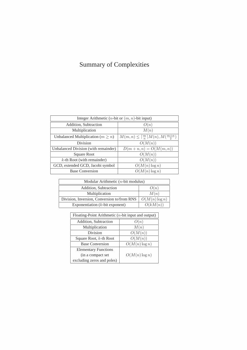
Summary of Complexities
Integer Arithmetic (n-bit or (m,n)-bit input)
Addition, Subtraction O(n)
Multiplication M(n)
Unbalanced Multiplication (m ≥ n) M(m,n) ≤ ⌈mn ⌉M(n),M(m+n
2 )
Division O(M(n))
Unbalanced Division (with remainder) D(m + n, n) = O(M(m,n))
Square Root O(M(n))
k-th Root (with remainder) O(M(n))
GCD, extended GCD, Jacobi symbol O(M(n) log n)
Base Conversion O(M(n) log n)
Modular Arithmetic (n-bit modulus)
Addition, Subtraction O(n)
Multiplication M(n)
Division, Inversion, Conversion to/from RNSO(M(n) log n)
Exponentiation (k-bit exponent) O(kM(n))
Floating-Point Arithmetic (n-bit input and output)
Addition, Subtraction O(n)
Multiplication M(n)
Division O(M(n))
Square Root,k-th Root O(M(n))
Base Conversion O(M(n) log n)
Elementary Functions(in a compact set O(M(n) log n)
excluding zeros and poles)


