Module 14: Savings Verification - Department Of Energy Energy Audit Training...Module 14: Savings...

Module 14: Savings Verification

Energy Audit Supervising Engineers Course Page 14.1


14.1 An Overview of Measurement and Verification (M&V) The central purpose of M&V is to verify the energy savings achieved by building retrofits, either to satisfy internal financial accounting and reporting requirements, or to meet the terms of third-party contracts for project implementation and management.

14.1.1 Working Definitions

The statistical analysis of energy consumption is commonly done for two reasons:

Measurement and Verification: this is a process of quantifying energy consumption before and after an energy conservation measure is implemented in order to verify and report on the level of savings actually achieved.

Monitoring and Targeting: this is a management technique that can—and should—be utilized with or without specific facility retrofits in order to ―keep operations efficient‖, and to ―monitor utility costs‖; these are management strategies designed to drive energy costs downwards as a continuous improvement cycle.

The statistical principles that are used are the same regardless of the purpose of the analysis. Because of its importance in energy performance contracts, and increasingly, in Clean Development Mechanism (CDM – under the Kyoto Protocol) projects involving greenhouse gas emission reduction credits, M&V methodology has been standardized in the International Performance Measurement and Verification Protocol (IPMVP).

14.1.2 Why Measure & Verify?

M & V is an additional cost in the retrofit project—what is the payoff? The IPMVP offers six answers to this question:

M & V increases energy savings.

M & V reduces the cost of financing projects.

M & V encourages better project engineering.

M & V helps to demonstrate and capture the value of reduced emissions from energy efficiency and renewable energy investments.

Learning Objectives

After completing this module, you will be able to: Identify the key concepts involved in savings verification;

Define the kinds of data required for energy performance analysis, and analyze energy consumption as a function of degree-days using linear regression;

Define the fundamental relationship for determining savings for a given ECM;

Describe the elements of a verification plan;

Describe and select from the four methods of savings verification; Identify the data and information required to define base year conditions; Describe techniques for developing an energy performance model; Apply adjustments to the base year conditions.


Page 14.2 Energy Audit Supervising Engineers Course

M & V increases public understanding of energy management as a public policy tool.

M & V helps organizations promote and achieve resource efficiency and environmental objectives.

Spend more to reduce costs? . . . This isn‘t a contradiction in terms. The IPMVP explains that a thorough M & V process designed into the project helps to reduce the total cost of a financed project by:

Increasing the confidence of funders that their investments will result in a savings stream sufficient to make debt payments

Thereby reducing the risk associated with the investment

Thereby reducing the expected rate of return of the investment—and your costs of borrowing.

14.1.3 General Approach to M&V – The IPMVP

In principle, M&V simply quantifies energy savings by comparing consumption before and after the retrofit. The ―before‖ case is defined as the ―baseline performance‖, and the ―after‖ case is referred to as the post-installation period. In its simplest form,

Savings = (Baseline Energy Use)adjusted – (Post-installation energy use)

The complicating factors concern:

what adjustments to the Baseline performance are required, and how are they carried out;

what measurements are required to determine post-installation performance, and how are they carried out.

The International Performance Measurement & Verification Protocol (IPMVP), published by the US Department of Energy, defines four approaches to M&V that determine how these factors are addressed. These approaches are termed M&V Options A, B, C and D. A critical decision in M&V planning is the selection of one of these options. M&V Options IPMVP M&V Options A, B, C and D are summarized in Table 14.1. They differ one from another in terms of:

the degree to which the retrofit can be measured separately from other facility components;

the extent to which performance variables can be measured. Option A applies to a retrofit or system level assessment where performance or operational factors can be spot or short-term measured during the baseline and post-installation periods. Factors that cannot or are not measured are ―stipulated‖, based on assumptions, analysis of historical performance, or manufacturer‘s data. Stipulation is the easiest and least expensive method of determining savings, but is also subject to the greatest level of uncertainty. Option B applies to a retrofit or system level assessment where performance or operational factors can be spot or short-term measured at the component or system level during the baseline and post-installation periods. In this Option, the performance of the retrofit can be measured separately from other measures or performance factors. No factors are stipulated; consequently, Option B involves more

IPMVP Volume I: Concepts and Options for Determining Energy and Water Savings and Volume II: Concepts and Practices for Improved Indoor Environmental Quality can be downloaded at no charge from www.ipmvp.org



end-use metering than Option A and is correspondingly both more expensive and less subject to uncertainty. Option C applies to the impact of a ―bundle‖ of retrofit measures on a facility. It relies on baseline and post-installation total building energy performance data typically obtained from the utility meter at the service entrance, and involves regression analysis against independent performance variables such as weather factors, facility usage, or production (as in water pumping stations or wastewater treatment facilities). Option D uses computer simulation models of component or whole-building energy consumption to determine project energy savings. Simulation inputs are linked to baseline and post-installation conditions; some of these inputs may be determined from performance metering before and after the retrofit. Long-term whole-building energy use data may be used to calibrate the simulation models.



Table 14.1: Overview of M&V Options Source: U.S. Department of Energy, M&V Guidelines: Measurement and

Verification for Federal Energy Projects

M&V Option

Performance and Operation Factors

1

Savings Calculation

M&V Cost2

Option A – Stipulated and measured factors

Based on a combination of measured and stipulated factors. Measurements are spot or short-term taken at the component or system level. The stipulated factor is supported by historical or manufacturer‘s data.

Engineering calculations, component, or system models.

Estimated range is 1% - 3%. Depends on number of points measured.

Option B – Measured factors (Retrofit isolation)

Based on spot or short-term measurements taken at the component or system level when variations in factors are not expected. Based on continuous measurements taken at the component or system level when variations are expected.

Engineering calculations, components, or system models.

Estimated range is 3% - 15%. Depends on number of points and term of metering.

Option C – Utility billing data analysis (whole building)

Based on long-term, whole-building utility meter, facility level, or sub-meter data.

Based on regression analysis of utility billing meter data.

Estimated range is 1% - 10%. Depends on complexity of billing analysis.

Option D – Calibrated computer simulation

Computer simulation inputs may be based on several of the following: engineering estimates; spot, short-, or long-term measurements of system components; and long-term, whole-building utility meter data.

Based on computer simulation model with whole-building and end-use data.

Estimated range is 3% - 10%. Depends on number and complexity of systems modelled.

1 Performance factors indicate equipment or system performance characteristics such

as kW/ton for a chiller or watts/fixture for lighting; operating factors indicate equipment or system operating characteristics such as annual cooling ton-hours for chillers or operating hours for lighting. 2 M&V costs are expressed as a percentage of measure or project energy savings.



14.2 A Statistical Basis for M&V

11.2.1 Relating energy use to weather As a basis for our analysis we must establish a simple but physical relationship between energy use and weather in a building. In simple terms, the energy required to heat the building during the heating season is equal to the heat lost from the building into the surrounding environment, through building walls, windows, and vents; and the energy required to cool the building in the cooling season is equal to the heat gained from the surrounding environment. In each case, the internal heat load is a factor—subtracting from the heat requirements or adding to the cooling requirements.

The rate at which heat loss or gain occurs is determined mainly by two key factors: the temperature difference driving force, being the difference between the indoor and outdoor temperature; and the thermal performance of the building.

A convenient way of quantifying this driving force is the heating degree day (HDD) and the cooling degree day (CDD). The HDD is defined as the sum of the differences of the daily mean temperature from a reference temperature, such as 18

oC (or

whatever temperature represents the thermal neutral point—at which neither heating

Notes to Table 14.1 1. Option A—partial retrofit isolation with stipulation—is best used when:

the magnitude of savings is relatively low for the entire project or the portion of the project to which this M&V Option is applied;

the risk of not achieving projected savings is low, or ESCO payments are not directly tied to the actual savings.

2. Option B—retrofit isolation—is typically used when:

energy savings from equipment replacement projects are less than 20% of the total facility energy use;

energy savings arising from individual measures must be determined;

interactive effects of multiple measures are deemed unimportant;

the independent variables that affect energy use—for example, operating schedule—are neither complex nor difficult to monitor;

sub-meters already exist to measure the energy use of the systems being considered for retrofit.

3. Option C—whole building, billing analysis—is used when:

the retrofit project is complex, involving a number of systems;

predicted energy savings are relatively large (greater than 10% to 20% of total facility energy use);

the measurement of energy savings arising from individual measures is not required;

interactive effects of multiple measures are to be included in the analysis;

the independent variables that affect energy use may be complex, and are difficult or expensive to monitor.

4. Option D—calibrated simulation—is used in situations similar to Option C, or when:

new construction projects are involved (i.e. there is no historical data for baseline determination);

energy savings per measure are required;

Option C tools cannot assess particular measures or their interactions when complex baseline adjustments are anticipated.



nor cooling is required to maintain the desired indoor temperature—for the building in question), for each day on which the temperature falls below that value in a specified period. (For any building, there is an outside temperature at which no heat needs to be added by the temperature control plant in order to maintain the set point. This is the thermal neutral temperature at which normal activity—heat given off by people, lights, and other equipment—generates sufficient heat to just maintain the desired temperature in spite of air changes and heat loss through the building envelope. The monitoring methods addressed later in this section require the use of this thermal neutral as the base temperature, rather than necessarily 18

oC.)

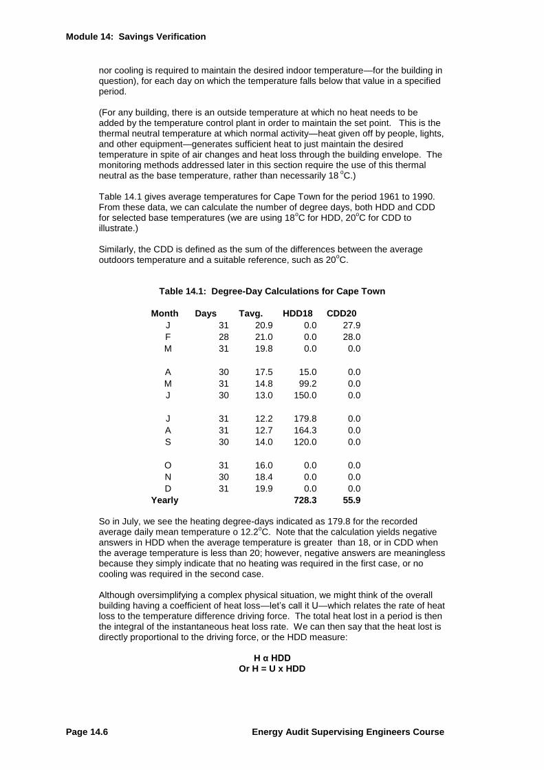
Table 14.1 gives average temperatures for Cape Town for the period 1961 to 1990. From these data, we can calculate the number of degree days, both HDD and CDD for selected base temperatures (we are using 18

oC for HDD, 20

oC for CDD to

illustrate.) Similarly, the CDD is defined as the sum of the differences between the average outdoors temperature and a suitable reference, such as 20

oC.

Table 14.1: Degree-Day Calculations for Cape Town

Month Days Tavg. HDD18 CDD20

J 31 20.9 0.0 27.9

F 28 21.0 0.0 28.0

M 31 19.8 0.0 0.0

A 30 17.5 15.0 0.0

M 31 14.8 99.2 0.0

J 30 13.0 150.0 0.0

J 31 12.2 179.8 0.0

A 31 12.7 164.3 0.0

S 30 14.0 120.0 0.0

O 31 16.0 0.0 0.0

N 30 18.4 0.0 0.0

D 31 19.9 0.0 0.0

Yearly 728.3 55.9 So in July, we see the heating degree-days indicated as 179.8 for the recorded average daily mean temperature o 12.2

oC. Note that the calculation yields negative

answers in HDD when the average temperature is greater than 18, or in CDD when the average temperature is less than 20; however, negative answers are meaningless because they simply indicate that no heating was required in the first case, or no cooling was required in the second case. Although oversimplifying a complex physical situation, we might think of the overall building having a coefficient of heat loss—let‘s call it U—which relates the rate of heat loss to the temperature difference driving force. The total heat lost in a period is then the integral of the instantaneous heat loss rate. We can then say that the heat lost is directly proportional to the driving force, or the HDD measure:

H α HDD Or H = U x HDD



with the constant of proportion being the heat transfer coefficient of the building. This provides a theoretical basis for the empirical expectation that energy plotted against HDD is a straight line. A more rigorous development of this relationship follows below. What we have established so far is that it is reasonable to plot energy against HDD or CDD and to expect a straight line. Indeed, that is what is commonly found, with a straight line produced of the form:

y = mx + c

where c, the intercept, and m, the slope, are empirical coefficients. For our working example this is shown in Figure 14.1 in which the base year (1999/2000) heating season data are used. In fact, there are three features in Figure 14.1. Apart from c and m, another feature is the scatter. The graph points in Figure 14.1 represent the energy consumption on a billing period basis, plotted against the HDD for that period As expected, the kWh energy consumed increases with HDD, although there is some scatter, in particular one or two points that fall well below the trend established by the others.

Figure 14.1 Energy Consumption vs. HDD Scatter Plot

11.2.2 Heating Requirements and Weather – A Rigorous Development of the Relationship The heat needs of a building are primarily determined by the need to maintain the temperature of the building by adding heat through the heating system to offset heat lost through the building envelope and ventilation. The relationship between heat requirement and temperature is expressed as follows:

H = U A (Ti-To) + Cp N V (Ti-To) (Equation 14.1)

where: H is the heat input to the building per unit of time

Baseline Energy vs. HDD

0

2000

4000

6000

8000

10000

12000

14000

16000

18000

20000

0 200 400 600 800 1000

HDD (oC)

To

tal kW

h



U is the heat transfer coefficient of the building envelope, taking into account its components such as glazing, interior wall finish, insulation, exterior wall, etc. A is the external area of the building envelope Cp is the specific heat of air N is the number of air changes of per unit of time V is the volume of the building being ventilated Ti-To is the difference between the inside and outside temperatures.

The two terms of this equation represent heat requirements to overcome heat loss through the building envelope, and to replace heat lost by ventilation respectively. Algebraically they can be combined to simplify the equation, as follows:

H = (U A + Cp N V )(Ti-To) (Equation 14.2)

U, A, Cp, N, and V are all characteristic constants of the building, and usually T i is controlled at a constant set value. Therefore, the only variable in the equation is To, and it may be higher or lower than the inside temperature depending on the season. When To is less than Ti, H is a positive number indicating that heat must be added to the building—the heating season; conversely when To is greater than Ti , H is a negative number indicating that heat must be removed from the building—the cooling season. When degree-days are used as the determinant of heat load, equation 14.2 becomes:

H = (U A + Cp N V ) x degree-days + c (Equation 14.3)

which you will recognize as the equation of a straight line, as in Figure 14.2, when H is plotted against degree-days, having a slope = (U A + Cp N V) and an intercept on the y-axis = c. This constant c is the ‗no load‘ energy provided whatever the weather conditions by such things as office equipment, the losses from the boiler, lighting, and people.

CUSUM is an application of the regression model seen previously in its use for savings verification. As a management tool, the relationship between energy consumption and key determining parameters, HDD in this example, is used to monitor current performance against the standard of the baseline relationship. We have seen how to do linear regression previously. For the example in this discussion, we know that no measures were implemented until the end of the first

(UA + Cp N V) = slope

Degree-days

H

} c

Figure 14.2: Relation between degree-days

and heat load



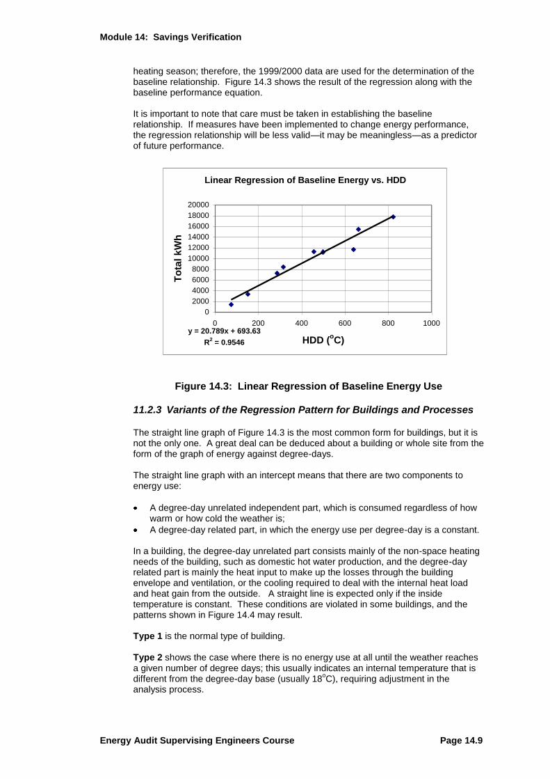
heating season; therefore, the 1999/2000 data are used for the determination of the baseline relationship. Figure 14.3 shows the result of the regression along with the baseline performance equation. It is important to note that care must be taken in establishing the baseline relationship. If measures have been implemented to change energy performance, the regression relationship will be less valid—it may be meaningless—as a predictor of future performance.

Figure 14.3: Linear Regression of Baseline Energy Use

11.2.3 Variants of the Regression Pattern for Buildings and Processes

The straight line graph of Figure 14.3 is the most common form for buildings, but it is not the only one. A great deal can be deduced about a building or whole site from the form of the graph of energy against degree-days.

The straight line graph with an intercept means that there are two components to energy use:

A degree-day unrelated independent part, which is consumed regardless of how warm or how cold the weather is;

A degree-day related part, in which the energy use per degree-day is a constant.

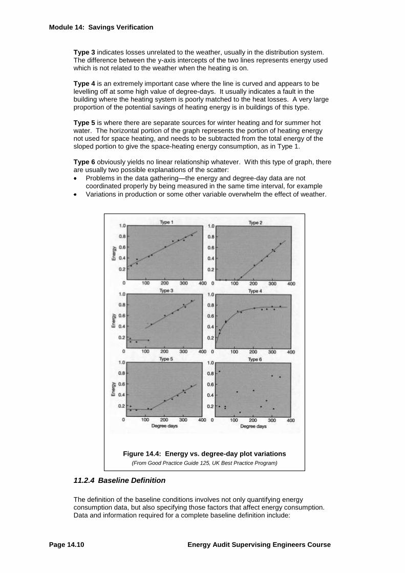
In a building, the degree-day unrelated part consists mainly of the non-space heating needs of the building, such as domestic hot water production, and the degree-day related part is mainly the heat input to make up the losses through the building envelope and ventilation, or the cooling required to deal with the internal heat load and heat gain from the outside. A straight line is expected only if the inside temperature is constant. These conditions are violated in some buildings, and the patterns shown in Figure 14.4 may result. Type 1 is the normal type of building. Type 2 shows the case where there is no energy use at all until the weather reaches a given number of degree days; this usually indicates an internal temperature that is different from the degree-day base (usually 18

oC), requiring adjustment in the

analysis process.

Linear Regression of Baseline Energy vs. HDD

y = 20.789x + 693.63

R2 = 0.9546

0

2000

4000

6000

8000

10000

12000

14000

16000

18000

20000

0 200 400 600 800 1000

HDD (oC)

To

tal

kW

h



Type 3 indicates losses unrelated to the weather, usually in the distribution system. The difference between the y-axis intercepts of the two lines represents energy used which is not related to the weather when the heating is on. Type 4 is an extremely important case where the line is curved and appears to be levelling off at some high value of degree-days. It usually indicates a fault in the building where the heating system is poorly matched to the heat losses. A very large proportion of the potential savings of heating energy is in buildings of this type. Type 5 is where there are separate sources for winter heating and for summer hot water. The horizontal portion of the graph represents the portion of heating energy not used for space heating, and needs to be subtracted from the total energy of the sloped portion to give the space-heating energy consumption, as in Type 1. Type 6 obviously yields no linear relationship whatever. With this type of graph, there are usually two possible explanations of the scatter:

Problems in the data gathering—the energy and degree-day data are not coordinated properly by being measured in the same time interval, for example

Variations in production or some other variable overwhelm the effect of weather.

11.2.4 Baseline Definition

The definition of the baseline conditions involves not only quantifying energy consumption data, but also specifying those factors that affect energy consumption. Data and information required for a complete baseline definition include:

Figure 14.4: Energy vs. degree-day plot variations (From Good Practice Guide 125, UK Best Practice Program)



Energy consumption data:

Electricity consumption information—bills and derived information (kW, kVA, PF), meter readings (especially for subsystem measurements), demand profiles;

Fuel consumption information—bills, monthly consumption profiles, fuel-by-fuel data (quantity, calorific value of fuels consumed, etc.);

Water consumption information

Other energy sources—e.g. purchased steam, etc.

Independent variable data:

Weather factors—HDD or CDD;

Facility occupancy or usage data—operating hours, number of patrons, etc.;

Throughput or production—as in volume of water pumped or wastewater treated;

Space conditions—set points on heating/cooling systems;

Equipment malfunctions—records of outages.

Baseline Adjustments The fundamental relationship for savings verification includes ―adjustment‖ of the baseline performance. Baseline adjustments potentially represent the most contentious aspect of energy performance contracts, and may be the most difficult aspect of savings verification to quantify. Simply put, ―adjustment‖ places the baseline energy performance on a ―level playing field‖ with post-installation performance in terms of those independent variables that affect energy consumption. ESCOs must specify as part of their M&V plan how they will adjust the baseline if the post-installation operating conditions are different from those used to determine the baseline. These specifications should address the independent variables listed above, as relevant to the project. The following are examples of baseline adjustments:

Changes in weather or occupancy: adjustments might include recalculating the baseline consumption rates using post-installation period weather data (HDD or CDD) or occupancy data based on a mathematical expression of how energy consumption depends on these factors;

Changes in operating schedule or tenant improvements: the real impact of the retrofit project is independent of decreases or increases in operating hours of the facility or system and, therefore, the baseline consumption needs to be scaled up or down to correspond to such changes if any occur; similarly, tenant improvements—new plug loads, improved lighting levels unrelated to the retrofit itself, etc.—that may increase energy consumption in the post-installation period must be separated from the post-installation period performance.

Changes in the actual function of the facility—office space being converted to storage, for example—and their impact on energy performance separate and apart from the retrofit, need to be quantified as adjustments to baseline performance.

The extent to which baseline adjustments need to be considered depends to some extent on the M&V Option being employed:

Baseline adjustments are less likely to be needed when M&V Option A is being used since many of the performance factors are stipulated.



Option B or retrofit isolation involves metering of energy consumption pre- and post-installation; non-metered factors that impact on energy performance therefore need to be applied to the measured baseline consumption.

Option C involves regression analysis to determine a functional relationship between energy consumption and independent variables; adjustment to the baseline performance for changes in these variables is typically carried out by using that functional relationship or performance model.

Option D accommodates adjustment within the simulation model itself; once calibrated using actual or typical data, no other adjustments should be required.

14.3 A Framework for Verification

14.3.1 M&V Process Flow Chart

Figure 14.5 is a flow chart to outline the steps involved in planning and implementing an M&V process. A planning template follows in Figure 14.6.

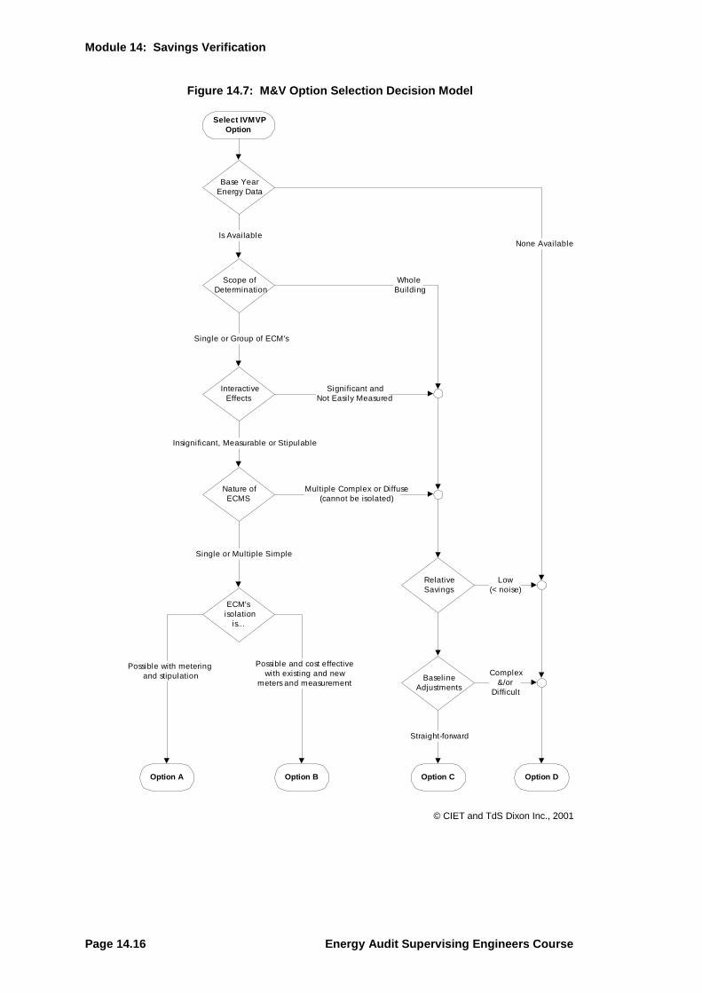
14.3.2 M&V Option Selection Decision Model Figure 14.7 is a decision tree for the selection of the IPMVP Option to be employed in a given project. The selection of an M&V Method from the Options described in the IPMVP is based on:

project costs;

expected savings;

complexity and number of measures installed;

anticipated changes to post-installation facility or system usage;

tolerance for uncertainty or risk of savings being achieved;

risk allocation between the owner and the contractor.

There is a trade-off between the cost of doing M&V and uncertainty. In general, the lower the acceptable level of uncertainty, the higher the cost. For example, a project with anticipated annual savings of R2,500,000 and estimated uncertainty of 20% has a savings risk of R500,000; if an M&V program costing R125,000 can reduce that risk to 10% or R250,000, there is a cost/benefit ratio of 2/1 for the M&V program that may be deemed a good investment. This kind of analysis needs to be done to evaluate the cost of reducing risk.



Figure 14.5: M&V Process Flow Chart

M&V Process

Prepare the

Organization

Implement the

ECM's

Implement the

M&V Plan

Design Energy

Savings Program

Identify, Select

and Assess the

ECM's

Apply M&V

Performance

Model to Ongoing

Management

Select

Implementation

Method

Save !

Define Ongoing

M&V Activities

Define & Specify

Metering

Equipment

Test Performance

Model for

Uncertainty etc..

Develop

Performance

Model

Define Post ECM

Period

Define Base Year

Performance

Select IPMVP

Option

Prepare the

M&V Plan

Model OK

Revise

Performance

Model

NO,

Needs Revision

Yes

NO,

Approach

not

Suitable

Document the

M&V Plan

Done

Implement the

ECM'sImplement the

ECM'sPrepare the

M&V Plan

© CIET and TdS Dixon Inc., 2001



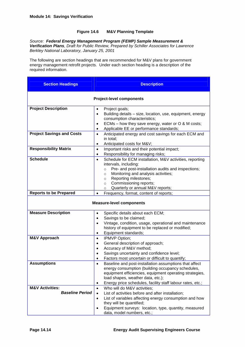
Figure 14.6 M&V Planning Template

Source: Federal Energy Management Program (FEMP) Sample Measurement & Verification Plans, Draft for Public Review, Prepared by Schiller Associates for Lawrence Berkley National Laboratory, January 25, 2001 The following are section headings that are recommended for M&V plans for government energy management retrofit projects. Under each section heading is a description of the required information.

Section Headings

Description

Project-level components

Project Description Project goals;

Building details – size, location, use, equipment, energy consumption characteristics;

ECMs – how they save energy, water or O & M costs;

Applicable EE or performance standards;

Project Savings and Costs Anticipated energy and cost savings for each ECM and in total;

Anticipated costs for M&V;

Responsibility Matrix Important risks and their potential impact;

Responsibility for managing risks;

Schedule Schedule for ECM installation, M&V activities, reporting intervals, including: o Pre- and post-installation audits and inspections; o Monitoring and analysis activities; o Reporting milestones; o Commissioning reports; o Quarterly or annual M&V reports;

Reports to be Prepared Frequency, format, content of reports;

Measure-level components

Measure Description Specific details about each ECM;

Savings to be claimed;

Vintage, condition, usage, operational and maintenance history of equipment to be replaced or modified;

Equipment standards;

M&V Approach IPMVP Option;

General description of approach;

Accuracy of M&V method;

Savings uncertainty and confidence level;

Factors most uncertain or difficult to quantify;

Assumptions Baseline and post-installation assumptions that affect energy consumption (building occupancy schedules, equipment efficiencies, equipment operating strategies, load shapes, weather data, etc.);

Energy price schedules, facility staff labour rates, etc.;

M&V Activities: Baseline Period

Who will do M&V activities;

List of activities before and after installation;

List of variables affecting energy consumption and how they will be quantified;

Equipment surveys: location, type, quantity, measured data, model numbers, etc.;



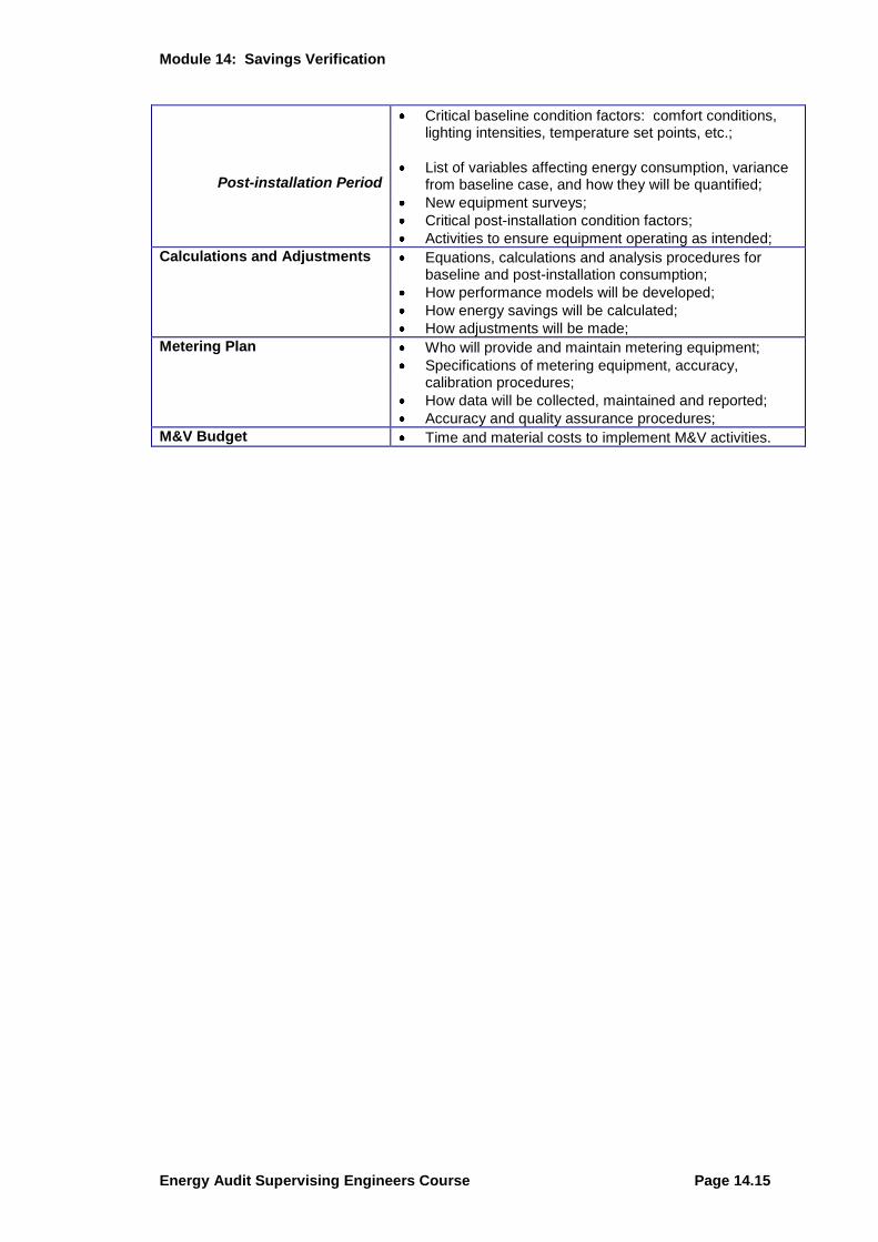
Post-installation Period

Critical baseline condition factors: comfort conditions, lighting intensities, temperature set points, etc.;

List of variables affecting energy consumption, variance from baseline case, and how they will be quantified;

New equipment surveys;

Critical post-installation condition factors;

Activities to ensure equipment operating as intended;

Calculations and Adjustments Equations, calculations and analysis procedures for baseline and post-installation consumption;

How performance models will be developed;

How energy savings will be calculated;

How adjustments will be made;

Metering Plan Who will provide and maintain metering equipment;

Specifications of metering equipment, accuracy, calibration procedures;

How data will be collected, maintained and reported;

Accuracy and quality assurance procedures;

M&V Budget Time and material costs to implement M&V activities.



Figure 14.7: M&V Option Selection Decision Model

Base Year

Energy Data

Is AvailableNone Available

Select IVMVP

Option

Interactive

Effects

Scope of

Determination

Nature of

ECMS

Whole

Building

Single or Group of ECM's

Significant and

Not Easily Measured

Insignificant, Measurable or Stipulable

Multiple Complex or Diffuse

(cannot be isolated)

Single or Multiple Simple

Possible and cost effective

with existing and new

meters and measurement

Option DOption COption BOption A

ECM's

isolation

is...

Relative

Savings

Low

(< noise)

Possible with metering

and stipulation Baseline

Adjustments

Straight-forward

Complex

&/or

Difficult

© CIET and TdS Dixon Inc., 2001



Worksheet 14.1: M&V Option Selection

1. Examine the municipal facility case assigned to your group. Make an initial selection of the M&V option best suited to the facility and the ECM‘s outlined.

Use the attached Option Selection Flowchart along with the Criteria for Selection from the FEMP M&V Guidelines and Best Application from IPMVP as follows:

Best Applications Option A IPMVP page 26 Option B IPMVP page 27 Option C IPMVP page 31 Option D IPMVP page 34 Criteria for Selection of M&V Approach: FEMP M&V Guidelines section 2.5.3, page 26

2. Provide reasons for your selection:

3. Clearly, a final option selection would require more detailed analysis. List any factors that may in further detailed analysis necessitate the use of another option. Identify which option may be required:



Worksheet 14.2: Responsibility Matrix worksheet

Financial Risks Management Strategy

Interest rates Neither the ESCO nor the agency has significant control over the prevailing interest rate. During all phases of the project interest rates will change with market conditions. Higher interest rates will increase project cost, finance term, or both. The timing of the Delivery Order signing may affect the available interest rate and project cost. Clarify when the interest rate is locked in, and if it is a fixed or variable rate.

Energy prices Neither the ESCO nor the agency has significant control over actual energy prices. For calculating savings, the value of the saved energy may either be constant, change at a fixed inflation rate, or float with market conditions. If the value changes with the market, falling energy prices place the ESCO at risk of failing to meet cost savings guarantees. If energy prices rise, there is a small risk to the agency that energy saving goals might not be met while the financial goals are. If the value of saved energy is fixed (either constant or escalated), the agency risks making payments in excess of actual energy cost savings.

Construction costs The ESCO is responsible for determining construction costs and defining a budget. In a fixed-price design/build contract, the agency assumes little responsibility for cost overruns. However, if construction estimates are significantly greater than originally assumed, the ESCO may find that the project or measure is no longer viable and drop it. In any design build contract the agency loses some design control. Clarify design standards and the design approval process (including changes), and how costs will be reviewed.

M&V costs The agency assumes the financial responsibility for M&V costs directly or though the ESCO. If the agency wishes to reduce M&V cost, it may do so by accepting less rigorous M&V activities with more uncertainty in the savings estimates. Clarify what performance is being guaranteed (equipment performance, operational factors, energy cost savings), and that the M&V plan is detailed enough to satisfactorily verify it.

Delays Both the ESCO and the agency can cause delays. Failure to implement a viable project in a timely manner costs the agency in the form of lost savings, and can add cost to the project. Clarify schedule, and how delays will be handled.

Major changes in facility The agency (or Congress) controls major changes in facility use, including closure. Clarify responsibilities in the event of a premature facility closure, loss of funding, or other major change.



Operational Risks Management Strategy

Operating hours The Agency generally has control over the operating hours. Increases and decreases in operating hours can show up as increases or decreases in ―savings‖ depending on the M&V method (e.g. operating hours times improved efficiency of equipment vs. whole building utility analysis). Clarify if operating hours are to be measured or stipulated, and what is the impact if they change. If the operating hours are stipulated, the baseline should be carefully documented and agreed to by both parties.

Load Equipment loads can change over time. The agency generally has control over hours of operation, conditioned floor area, intensity of use (e.g. changes in occupancy or level of automation). Changes in load can show up as increases or decreases in ―savings‖ depending on the M&V method. Clarify if equipment loads are to be measured or stipulated and what is the impact if they change. If the equipment loads are stipulated, the baseline should be carefully documented and agreed to by both parties.

Weather A number of energy efficiency measures are affected by weather. Neither the ESCO nor the agency has control over the weather. Changes in weather can increase or decrease ―savings‖ depending on the M&V method (e.g. equipment run hours times efficiency improvement vs. whole building utility analysis). If weather is ―normalized,‖ actual savings could be less than payments for a given year, but will ―average out‖ over the long run. Weather corrections to the baseline or ongoing performance should be clearly specified and understood.

User participation Many energy conservation measures require user participation to generate savings (e.g. control settings). The savings can be variable and the ESCO may be unwilling to invest in these measures. Clarify what degree of user participation is needed, and utilize monitoring and training to mitigate risk. If performance is stipulated, document and review assumptions carefully, and consider M&V to confirm the capacity to save (e.g. confirm that the controls are functional).



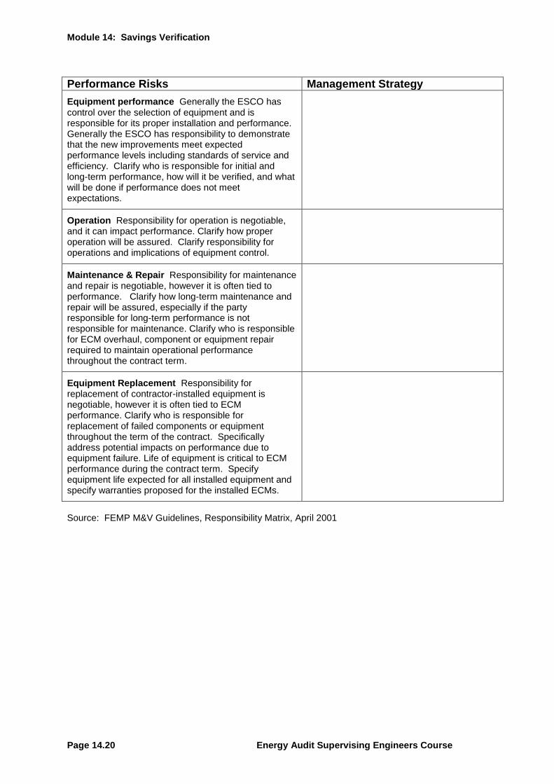
Performance Risks Management Strategy

Equipment performance Generally the ESCO has control over the selection of equipment and is responsible for its proper installation and performance. Generally the ESCO has responsibility to demonstrate that the new improvements meet expected performance levels including standards of service and efficiency. Clarify who is responsible for initial and long-term performance, how will it be verified, and what will be done if performance does not meet expectations.

Operation Responsibility for operation is negotiable, and it can impact performance. Clarify how proper operation will be assured. Clarify responsibility for operations and implications of equipment control.

Maintenance & Repair Responsibility for maintenance and repair is negotiable, however it is often tied to performance. Clarify how long-term maintenance and repair will be assured, especially if the party responsible for long-term performance is not responsible for maintenance. Clarify who is responsible for ECM overhaul, component or equipment repair required to maintain operational performance throughout the contract term.

Equipment Replacement Responsibility for replacement of contractor-installed equipment is negotiable, however it is often tied to ECM performance. Clarify who is responsible for replacement of failed components or equipment throughout the term of the contract. Specifically address potential impacts on performance due to equipment failure. Life of equipment is critical to ECM performance during the contract term. Specify equipment life expected for all installed equipment and specify warranties proposed for the installed ECMs.

Source: FEMP M&V Guidelines, Responsibility Matrix, April 2001



14.4 Verification Applied

11.4.1 Determining Base Year Data and Conditions

Worksheet 14.3: Base Year Data and Conditions

Take a moment to list the base year data and conditions from Option C Example: Whole Building Multiple ECM Project on page 64 of the IPMVP.

With a checkmark, indicate the data actually used in the baseline determination.



11.4.2 Hierarchy of Available Energy Use Data

Worksheet 14.4: Hierarchy of Available Energy Use Data List and organize in the following table the kinds of information that you are aware of being currently available to describe the energy performance of facilities in your portfolio. This is a table that may be useful for summarizing information availability in the early stages of your M&V planning process.

Building1 System2 Data3 Source4

1 Building – for which facility or group of facilities does this information exist

2 System – for what energy consuming systems or specific devices does this information exist

3 Data – what kind of data is currently available (e.g. monthly energy costs, utility meter

readings) 4

Source – who has the data

Typically, in this table we will find a pattern structured as an hierarchy of information, in which:

Strategic level information can be derived from financial accounting systems—the utilities cost centre;

Portfolio information can be found in comparative energy consumption data for a group of similar buildings (rinks or recreation centres, for example);

Building performance data can be determined from utility billings, service entrance meter readings, building management system data, correlated with building use and weather data;

System information can be derived from name-plate data, run-time and schedule information, sub-metered data on specific energy consuming systems.



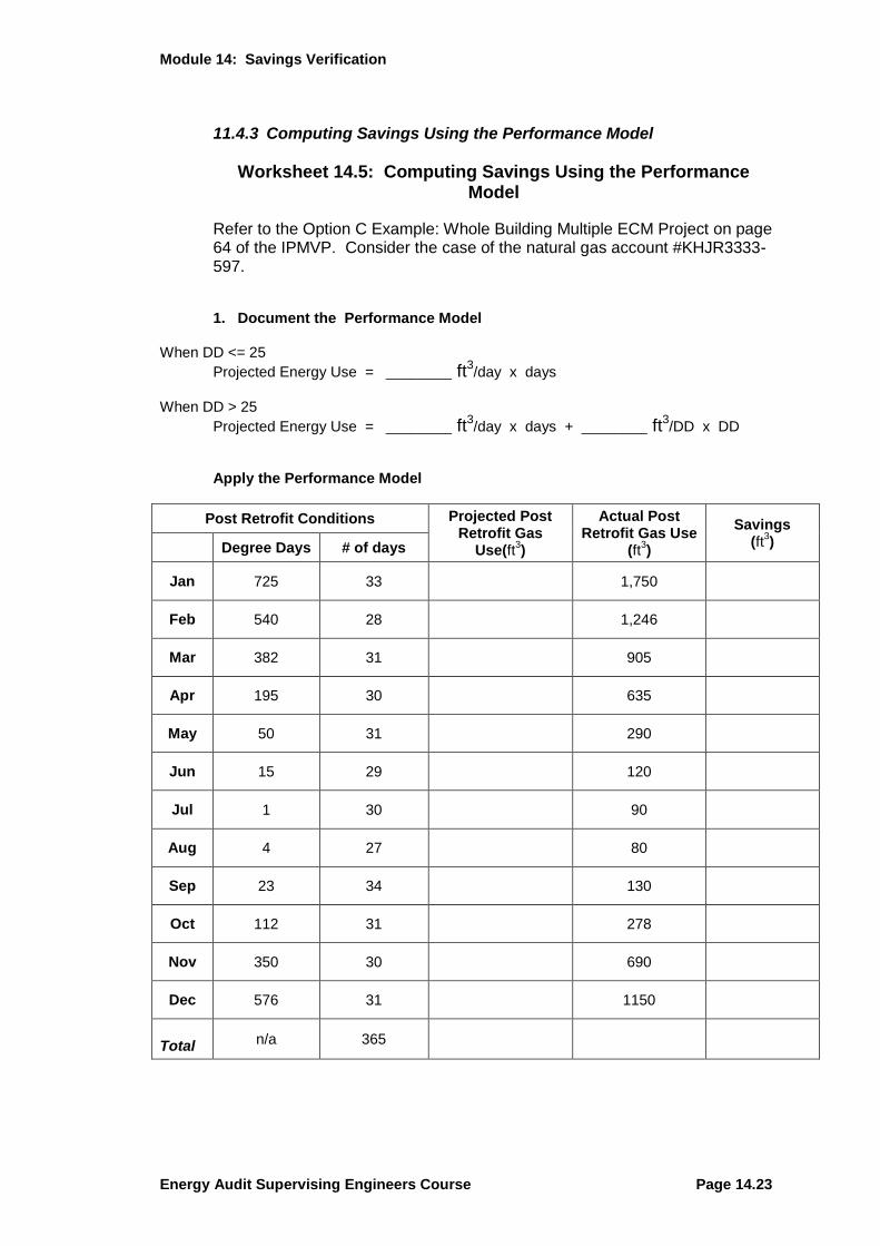
11.4.3 Computing Savings Using the Performance Model

Worksheet 14.5: Computing Savings Using the Performance Model

Refer to the Option C Example: Whole Building Multiple ECM Project on page 64 of the IPMVP. Consider the case of the natural gas account #KHJR3333-597. 1. Document the Performance Model

When DD <= 25

Projected Energy Use = ________ ft3/day x days

When DD > 25

Projected Energy Use = ________ ft3/day x days + ________ ft3/DD x DD

Apply the Performance Model

Post Retrofit Conditions Projected Post Retrofit Gas

Use(ft3)

Actual Post Retrofit Gas Use

(ft3)

Savings (ft

3) Degree Days # of days

Jan 725 33 1,750

Feb 540 28 1,246

Mar 382 31 905

Apr 195 30 635

May 50 31 290

Jun 15 29 120

Jul 1 30 90

Aug 4 27 80

Sep 23 34 130

Oct 112 31 278

Nov 350 30 690

Dec 576 31 1150

Total n/a 365



11.4.4 Non-Routine Adjustments

Worksheet 14.6: Non-routine Adjustments - Computing Savings with Non-Routine Adjustments

Consider the case of a gas fired pottery kiln being added to the school of the Option C example. Assume that the kiln was installed early in the July billing period. 1. Model the Adjustments When school is ―open‖

Kiln Energy Use = ______ ft3/day x days

When school is ―closed‖ Kiln Energy Use = 0 ft

3

2. Apply the Performance Model

Post Retrofit Conditions Projected Post Retrofit Gas

Use(ft3)

Actual Post Retrofit Gas

Use (ft3)

Adjustment for Kiln Use (ft

3)

Savings (ft

3) Degree

Days # of days

Jan 725 33

1,750

Feb 540 28

1,246

Mar 382 31

905

Apr 195 30

635

May 50 31

290

Jun 15 29

120

Jul 1 30

190

Aug 4 27

200

Sep 23 34

260

Oct 112 31

405

Nov 350 30

805

Dec 576 31

1210

Total n/a 365



11.4.5 Uncertainty in Verification

Worksheet 14.7: Uncertainty in Verification 1. For the selected Municipal Case identify the possible sources of uncertainty using the

M&V Option previously selected. Indicate whether you believe they can be quantified and rank them in order of significance in determining cost.

Source of Uncertainty Quantifiable? Rank

2. After this assessment would you consider changing the M&V option selected? If so to

which option and why? 3. Consider how much uncertainty would be tolerable / acceptable for each of the three

Cases.

Case Uncertainty Why

Recreation Centre

Municipal Office

Pumping Station



11.4.6 Cost Saving and Emission Reduction

Worksheet 14.8: Cost Saving & Emission Reduction

Basic Info Energy Demand

Baseline kWh kVA

Post Retrofit kWh kVA

Adjustment kWh kVA

Savings ( Baseline – Post Retrofit + Adjustment )

kWh kVA

Uncertainty % @ @ conf % @ @ conf

Rates

1st Block kWh @ R /kWh kVA @ R / kVA

2nd

Block kWh @ R /kWh kVA @ R / kVA

3rd

Block kWh @ R /kWh kVA @ R / kVA

Bill Calculation

1st Block Charges R R

2nd

Block Charges R R

3rd

Block Charges R R

Post Retrofit Bill R

Marginal Price R /kWh R /kW

Cost Savings R R

GHG Calculation

GHG Factor eq kg CO2/kWh eq kg CO2/kWh

kWh Saved kWh kWh

GHG Reduction (GHG Factor x kWh )

eq kg CO2 eq kg CO2



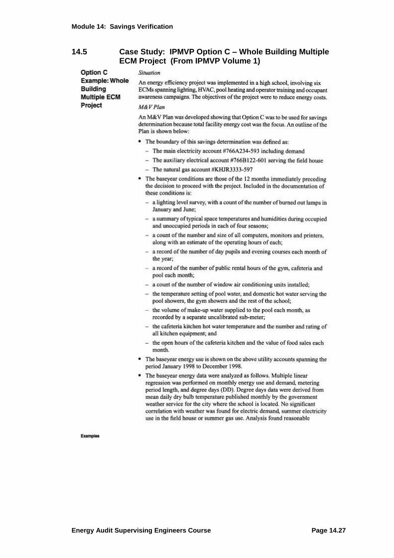
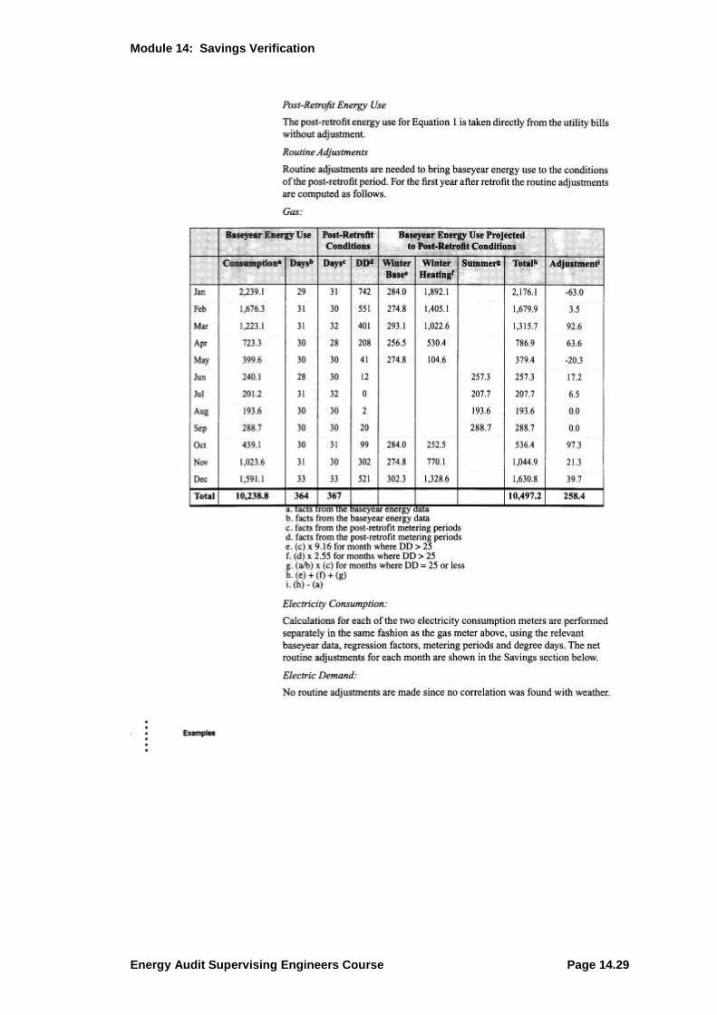
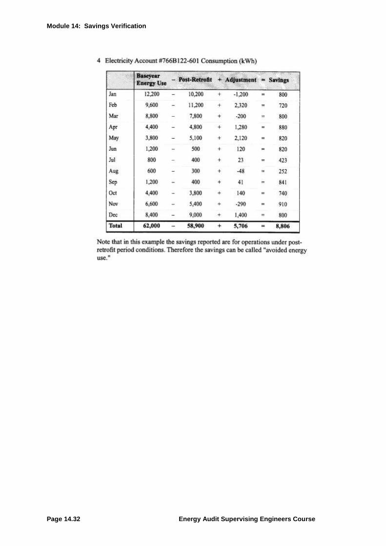
14.5 Case Study: IPMVP Option C – Whole Building Multiple ECM Project (From IPMVP Volume 1)













14.6 M & V Checklists

Worksheet 14.9: M & V Approach

Project site and measures are reasonably defined What savings will be claimed? (energy, interactive effects, O&M, rate

change, etc.)

M&V approach (A, B, C, D from IPMVP) is defined for each measure.

Baseline Equipment and Conditions Plan for defining existing equipment (inventory and performance) is

described Plan for defining space conditions (lighting intensity, temperatures, etc.) is

described How and why any baseline adjustments will be made is discussed.

Post-installation equipment and conditions Plan for defining new equipment (inventory and performance) is described Plan for defining space conditions (lighting intensity, temperatures, etc.) is

described

Annual verification and measurement activities are described Who will conduct the M&V activities and prepare M&V analyses and

documentation is described



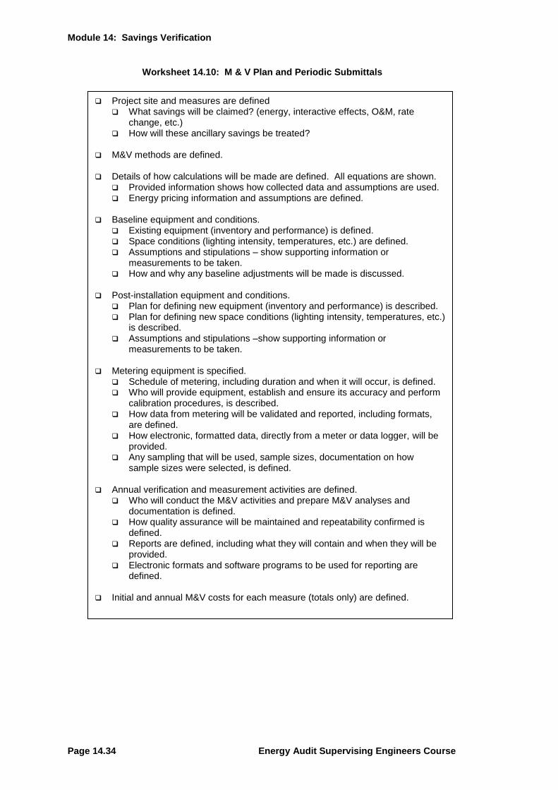
Worksheet 14.10: M & V Plan and Periodic Submittals

Project site and measures are defined What savings will be claimed? (energy, interactive effects, O&M, rate

change, etc.) How will these ancillary savings be treated?

M&V methods are defined. Details of how calculations will be made are defined. All equations are shown.

Provided information shows how collected data and assumptions are used. Energy pricing information and assumptions are defined.

Baseline equipment and conditions.

Existing equipment (inventory and performance) is defined. Space conditions (lighting intensity, temperatures, etc.) are defined. Assumptions and stipulations – show supporting information or

measurements to be taken. How and why any baseline adjustments will be made is discussed.

Post-installation equipment and conditions.

Plan for defining new equipment (inventory and performance) is described. Plan for defining new space conditions (lighting intensity, temperatures, etc.)

is described. Assumptions and stipulations –show supporting information or

measurements to be taken. Metering equipment is specified.

Schedule of metering, including duration and when it will occur, is defined. Who will provide equipment, establish and ensure its accuracy and perform

calibration procedures, is described. How data from metering will be validated and reported, including formats,

are defined. How electronic, formatted data, directly from a meter or data logger, will be

provided. Any sampling that will be used, sample sizes, documentation on how

sample sizes were selected, is defined. Annual verification and measurement activities are defined.

Who will conduct the M&V activities and prepare M&V analyses and documentation is defined.

How quality assurance will be maintained and repeatability confirmed is defined.

Reports are defined, including what they will contain and when they will be provided.

Electronic formats and software programs to be used for reporting are defined.

Initial and annual M&V costs for each measure (totals only) are defined.

Date post:	18-May-2018
Category:	Documents
Upload:	phamnguyet
View:	231 times
Download:	1 times

Module 14: Savings Verification - Department Of Energy Energy Audit Training...Module 14: Savings...

Documents