Monetary economics Michaª Brzoza-Brzezina

Introduction Data Moments SVARs Exercises VAR based evidence Long run e�ects of monetary policy

Empirical approach to monetary economicsMonetary economics

Michaª Brzoza-Brzezina

Warsaw School of Economics

1 / 60


Plan of the Presentation

1 Introduction

2 Data

3 Moments

4 SVARs

5 Exercises

6 VAR based evidence

7 Long run e�ects of monetary policy

2 / 60


Introduction

Basic facts about business cycles and monetary economics thatmodels are supposed to match:

monetary transmission from interest rates to output andin�ationmoments of data (variances, cyclical behavior, autoreggression)long run e�ects of monetary policy

This lecture:

Data preparationBusiness cycle momentsIdenti�cation of monetary policy shocks via SVARsShort-run e�ectst of monetary policy (SVAR evidence)Long-run e�ects of monetary policyEstimation of SVAR for monetary transmission

3 / 60



1 Introduction

2 Data

3 Moments

4 SVARs

5 Exercises



4 / 60


Why do we need data?

To estimate econometric models

To calibrate DSGE models

To estimate DSGE models

5 / 60


Business cycles

Models discussed in this lecture are (mainly) used to explainbusiness cycles

This means short and medium term co-movements ofmacroeconomic variables

We do not speak about growth here

If stationary RBC/ NK models are brought to the data, itshould have no trend

6 / 60


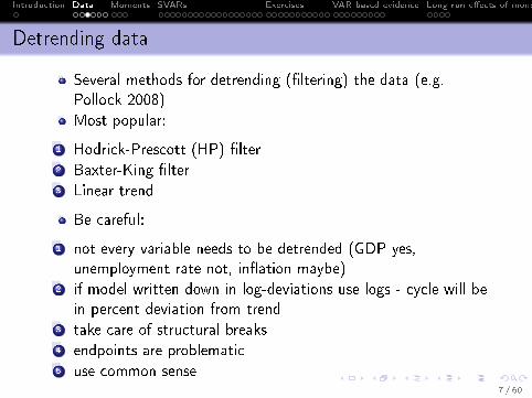
Detrending data

Several methods for detrending (�ltering) the data (e.g.Pollock 2008)

Most popular:

1 Hodrick-Prescott (HP) �lter2 Baxter-King �lter3 Linear trend

Be careful:

1 not every variable needs to be detrended (GDP yes,unemployment rate not, in�ation maybe)

2 if model written down in log-deviations use logs - cycle will bein percent deviation from trend

3 take care of structural breaks4 endpoints are problematic5 use common sense

7 / 60


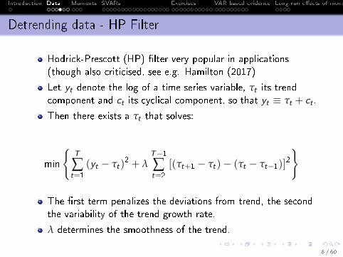
Detrending data - HP Filter

Hodrick-Prescott (HP) �lter very popular in applications(though also criticised, see e.g. Hamilton (2017)

Let yt denote the log of a time series variable, τt its trendcomponent and ct its cyclical component, so that yt ≡ τt + ct .

Then there exists a τt that solves:

min

{T

∑t=1

(yt − τt)2 + λ

T−1∑t=2

[(τt+1 − τt)− (τt − τt−1)]2

}

The �rst term penalizes the deviations from trend, the secondthe variability of the trend growth rate.

λ determines the smoothness of the trend.

8 / 60


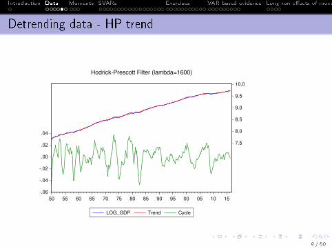
Detrending data - HP trend

-.06

-.04

-.02

.00

.02

.04

7.5

8.0

8.5

9.0

9.5

10.0

50 55 60 65 70 75 80 85 90 95 00 05 10 15

LOG_GDP Trend Cycle

Hodrick-Prescott Filter (lambda=1600)

9 / 60


Detrending data - linear trend

-.20

-.15

-.10

-.05

.00

.05

.10

7.5

8.0

8.5

9.0

9.5

10.0

50 55 60 65 70 75 80 85 90 95 00 05 10 15

LOG_GDP Trend Cycle

Hodrick-Prescott Filter (lambda=1600000000)

10 / 60



1 Introduction

2 Data

3 Moments

4 SVARs

5 Exercises



11 / 60


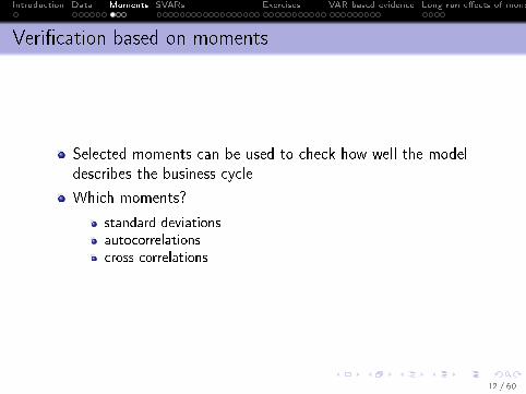
Veri�cation based on moments

Selected moments can be used to check how well the modeldescribes the business cycle

Which moments?

standard deviationsautocorrelationscross-correlations

12 / 60


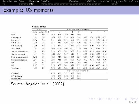
Example: US moments

Source: Angeloni et al. (2002)

13 / 60


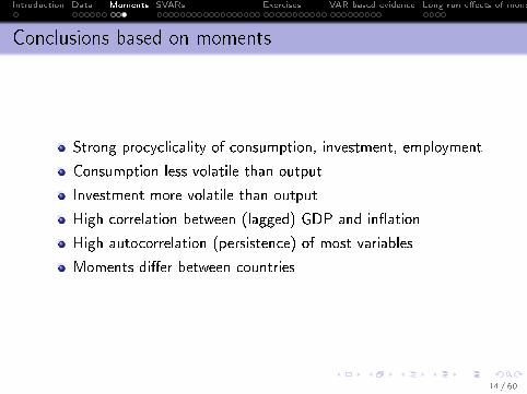
Conclusions based on moments

Strong procyclicality of consumption, investment, employment

Consumption less volatile than output

Investment more volatile than output

High correlation between (lagged) GDP and in�ation

High autocorrelation (persistence) of most variables

Moments di�er between countries

14 / 60



1 Introduction

2 Data

3 Moments

4 SVARs

5 Exercises



15 / 60


Some history

Macroeconometric modeling long, long time ago (1960-70's):

in the spirit of the Cowles Commission(very) big models with equations postulated by theory orempiricsso big that di�cult to understandnot necessarily good at forecastingcriticised on theoretical grounds (Lucas)

Two alternative approaches from the 1980's:

VAR (Sims 1980)RBC (Kydland & Prescott 1982) and NK (Woodford 1999)

16 / 60


Vector Autoregressions

Small, atheoretical models

Each variable is determined by lags of all variables

Highly popular i.a. in modeling monetary transmission

Parameters di�cult to interpret but provide causality tests,impulse responses, variance decompositions

17 / 60


Basic VAR

Consider a simple model of the form

y1,t = c1,1y1,t−1 + c1,2y2,t−1 + v1,t

y2,t = c2,1y1,t−1 + c2,2y2,t−1 + v2,t

or in matrix notation

yt = Cyt−1 + vt

This is a VAR(1). Note that using one lag is not restrictive,since further lags can be introduced as additional variables,e.g.:

(ytzt

)=

[C1 C2

I 0

] (yt−1zt−1

)+

(vt0

)18 / 60


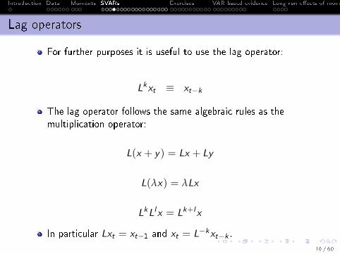
Lag operators

For further purposes it is useful to use the lag operator:

Lkxt ≡ xt−k

The lag operator follows the same algebraic rules as themultiplication operator:

L(x + y) = Lx + Ly

L(λx) = λLx

LkLlx = Lk+lx

In particular Lxt = xt−1 and xt = L−kxt−k .

19 / 60


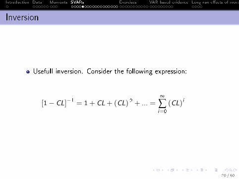
Inversion

Usefull inversion. Consider the following expression:

[1− CL]−1 = 1+ CL+ (CL) 2 + ... =∞

∑i=0

(CL)i

20 / 60


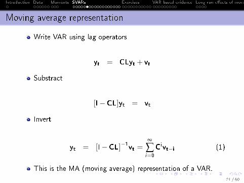
Moving average representation

Write VAR using lag operators

yt = CLyt + vt

Substract

[I−CL]yt = vt

Invert

yt = [I−CL]−1vt =∞

∑i=0

Civt−i (1)

This is the MA (moving average) representation of a VAR.

21 / 60


Reduced form VAR

Our estimated VAR is of the form

Iyt = Cyt−1 + vt

This is called reduced form because it does not provide anexplanation of the contemporaneous relationship betweenvariables

Still, can be useful:

ForecastingGranger causality testsStarting point for recovery of structural form

22 / 60


Reduced vs. structural form

The reduced form of a more general (structural) model, whichdoes not provide an explanation of the contemporaneousrelationship between variablesThese are hidden in the correlation structure of the VCVmatrix Σ.The reduced model has correlated shocks

correlation re�ects the contemporaneous relation of thevatriablescomplicates generation of impulse responsescomplicates generation of variance or historical decomposition

But we cannot estimate the structural model (regressorscorrelated with error term)The structural relationship cannot be identi�ed from thereduced model unless additional restrictions are imposedSee Amisano & Giannini �Topics in Structural VAR Modeling�or Favero �Applied Econometrics� for details

23 / 60


Identi�cation of the structural shocks

Write reduced form VAR:

yt =CLyt+ vt

Now premultiply by Θ such that ΘΣΘ′= I

Θyt = DLyt + ut

where ut = Θvt and DL = ΘCLNote that:

Θ imposes a structure on the contemporaneous relationshipbetween the variablesthe disturbances ut are now orthogonal

24 / 60


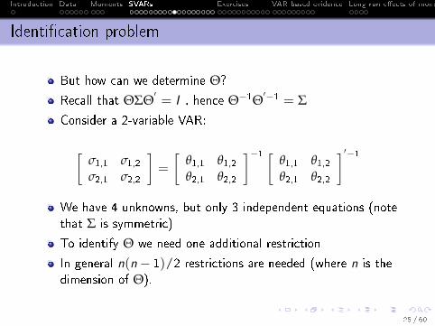
Identi�cation problem

But how can we determine Θ?

Recall that ΘΣΘ′= I , hence Θ−1Θ

′−1 = ΣConsider a 2-variable VAR:

[σ1,1 σ1,2σ2,1 σ2,2

]=

[θ1,1 θ1,2θ2,1 θ2,2

]−1 [θ1,1 θ1,2θ2,1 θ2,2

]′−1We have 4 unknowns, but only 3 independent equations (notethat Σ is symmetric)

To identify Θ we need one additional restriction

In general n(n− 1)/2 restrictions are needed (where n is thedimension of Θ).

25 / 60


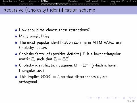
Recursive (Cholesky) identi�cation scheme

How should we choose these restrictions?

Many possibilities

The most popular identi�cation scheme in MTM VARs: useCholesky factors

Cholesky factor of (positive de�nite) Σ is a lower triangularmatrix Ξ, such that Σ = ΞΞ

′.

Cholesky identi�cation assumes Θ = Ξ−1 (which is lowertriangular too)

This implies ΘΣΘ′= I , so that disturbances ut are

orthogonal.

26 / 60


Cholesky identi�cation scheme

What does recursive identi�cation imply in terms ofeconomics?

It implies an ordering - which variable a�ects which in thecurrent period

Assume a standard monetary VAR with yt = [∆yt πt it ]′

Then Θ =

θ1,1 0 0θ1,2 θ2,2 0θ1,2 θ1,2 θ3,3

implies that:

eq 1: in�ation and interest rate have no current impact onoutputeq 2: interest rate has no current impact on in�ation (butoutput does)eq 3: all variables have a current period impact on the interestrate

Note that ordering of variables is crucial for the identi�cation.

27 / 60


Structural VARs - general approach

But Cholesky identi�cation is not the only possible oneMore generaly, one can write a structural model

Ayt = CLyt +But (2)

or yt=A−1CLyt +A−1But which implies vt = A−1But(where vt are reduced form residuals and ut are structuralshocks)This is the (so called) AB decomposition (Amisano & Giannini2011, Favero 2001)Matrix A determines contemporaneous relationship betweenvariablesMatrix B determines the impact of shocks on current-periodvariablesMany econometric softwares (e.g. Eviews, Gretl) allow forstructuralizing VARs by imposing restrictions on A and Bmatices.

28 / 60


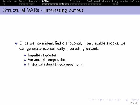
Structural VARs - interesting output

Once we have identi�ed orthogonal, interpretable shocks, wecan generate economically interesting output:

Impulse responsesVariance decompositionsHistorical (shock) decompositions

29 / 60


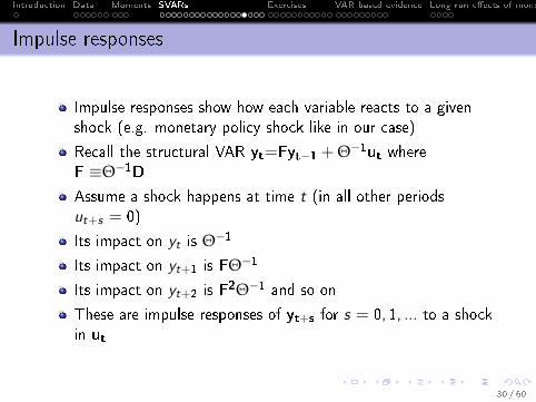
Impulse responses

Impulse responses show how each variable reacts to a givenshock (e.g. monetary policy shock like in our case)

Recall the structural VAR yt=Fyt−1 + Θ−1ut whereF ≡Θ−1DAssume a shock happens at time t (in all other periodsut+s = 0)

Its impact on yt is Θ−1

Its impact on yt+1 is FΘ−1

Its impact on yt+2 is F2Θ−1 and so on

These are impulse responses of yt+s for s = 0, 1, ... to a shockin ut

30 / 60


Forecast error variance decomposition

FEVD shows what share of forecast error variance can beexplained by a given shock

Recall the MA representation of the VAR model (1)

And apply the MA representation to the structural model

Then the error of forecasting yt+s (i.e. s periods into thefuture) is

yt+s − Etyt+s = ∑∞i=0 F i Θ−1ut+s−i − Et ∑∞

i=0 F i Θ−1ut+s−i

= ∑si=0 F i Θ−1ut+s−i + ∑∞

i=s+1 F i Θ−1ut+s−i − Et ∑si=0 F i Θ−1ut+s−i − Et ∑∞

i=s+1 F i Θ−1ut+s−i

= ∑si=0 F i Θ−1ut+s−i + ∑∞

i=s+1 F i Θ−1ut+s−i − 0−∑∞i=s+1 F i Θ−1ut+s−i = ∑s

i=0 F i Θ−1ut+s−i

31 / 60


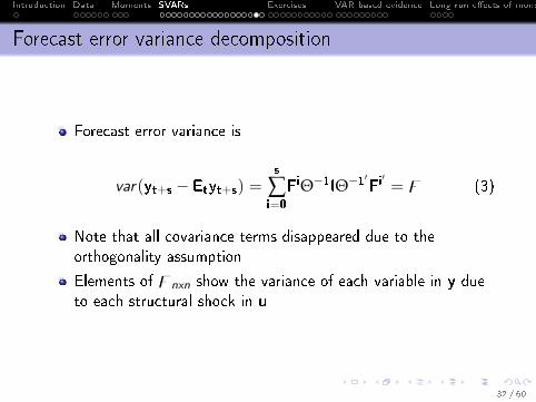
Forecast error variance decomposition

Forecast error variance is

var(yt+s − Etyt+s) =s

∑i=0

FiΘ−1IΘ−1′Fi′ = z (3)

Note that all covariance terms disappeared due to theorthogonality assumption

Elements of znxn show the variance of each variable in y dueto each structural shock in u

32 / 60


Historical (shock) decomposition

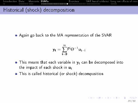
Again go back to the MA representation of the SVAR

yt =∞

∑i=0

FiΘ−1ut−i

This means that each variable in yt can be decomposed intothe impact of each shock in ut

This is called historical (or shock) decomposition

33 / 60



1 Introduction

2 Data

3 Moments

4 SVARs

5 Exercises



34 / 60


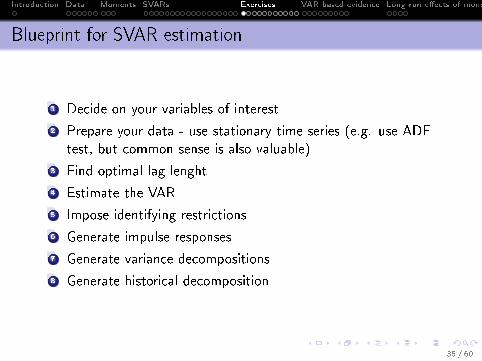
Blueprint for SVAR estimation

1 Decide on your variables of interest

2 Prepare your data - use stationary time series (e.g. use ADFtest, but common sense is also valuable)

3 Find optimal lag lenght

4 Estimate the VAR

5 Impose identifying restrictions

6 Generate impulse responses

7 Generate variance decompositions

8 Generate historical decomposition

35 / 60


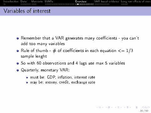
Variables of interest

Remember that a VAR generates many coe�cients - you can'tadd too many variables

Rule of thumb - # of coe�cients in each equation <= 1/3sample lenght

So with 60 observations and 4 lags use max 5 variables

Quarterly, monetary VAR:

must be: GDP, in�ation, interest ratemay be: money, credit, exchange rate

36 / 60


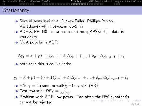
Stationarity

Several tests available: Dickey-Fuller, Phillips-Perron,Kwiatkowski�Phillips�Schmidt�ShinADF & PP: H0 - data has a unit root; KPSS: H0 - data isstationaryMost popular is ADF:

∆yt = α + βt + γyt−1 + δ1∆yt−1 + ...+ δp−1∆yt−p−1 + εt

note that this is equivalently:

yt = α + βt + (γ + 1)yt−1 + δ1∆yt−1 + ...+ δp−1∆yt−p−1 + εt

H0: γ = 0 (random walk); H1: γ < 0 (AR)Test statistic: DFT = γ̂

SE (γ̂).

Problem with ADF: low power. Too often the RW hypothesiscannot be rejected.

37 / 60


Finding optimal lag length for the VAR

Again, many tests available: LR, HQ, BIC, AIC

They all weight the bene�t from more lags (more information)against the cost (more parameters to estimate)

E.g. Akaike Information Criterion:

AIC = 2k − 2ln(L)

where k is number of parameters to be estimated and L is value ofmaximized likelihood function (i.e. probability of getting the data ygiven the estimated parameters θ:

L(θ|y) = P(y |θ)

38 / 60


(S)VAR estimation

Alternative approaches:

estimate ordinary VAR and impose Cholesky restrictions toidentify impulsesimpose restrictions before estimation (i.e. estimate SVAR)

Ordinary VAR is estimated with OLS equation by equation

SVAR with imposed restrictions is estimated with maximumlikelihood (system estimator)

39 / 60


IRFs, FEVD and historical decomposition

Once we identi�ed structural shocks impulse responses, FEVDor historical decomposition can be analyzed

40 / 60


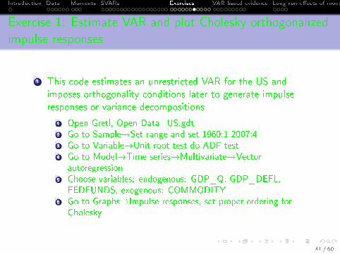
Exercise 1: Estimate VAR and plot Cholesky orthogonalizedimpulse responses

1 This code estimates an unrestricted VAR for the US andimposes orthogonality conditions later to generate impulseresponses or variance decompositions

1 Open Gretl, Open Data_US.gdt2 Go to Sample�Set range and set 1960:1-2007:43 Go to Variable�Unit root test do ADF test4 Go to Model�Time series�Multivariate�Vector

autoregression5 Choose variables: endogenous: GDP_Q, GDP_DEFL,

FEDFUNDS, exogenous: COMMODITY6 Go to Graphs�Impulse responses, set proper ordering for

Cholesky

41 / 60


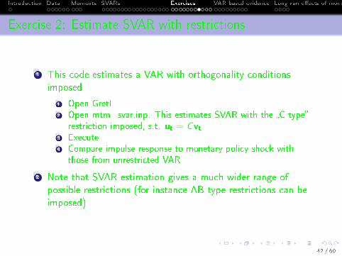
Exercise 2: Estimate SVAR with restrictions

1 This code estimates a VAR with orthogonality conditionsimposed

1 Open Gretl2 Open mtm_svar.inp. This estimates SVAR with the �C-type�

restriction imposed, s.t. ut = Cvt3 Execute4 Compare impulse response to monetary policy shock with

those from unrestricted VAR

2 Note that SVAR estimation gives a much wider range ofpossible restrictions (for instance AB type restrictions can beimposed)

42 / 60


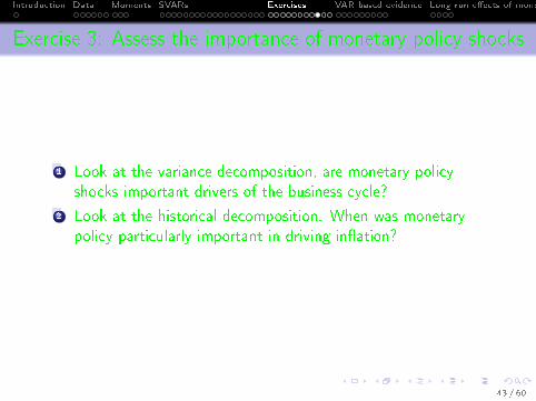
Exercise 3: Assess the importance of monetary policy shocks

1 Look at the variance decomposition, are monetary policyshocks important drivers of the business cycle?

2 Look at the historical decomposition. When was monetarypolicy particularly important in driving in�ation?

43 / 60


Exercise 4: Some VAR algebra in practice

1 Go back to unrestricted VAR (script mtm_var.inp). Show thatindeed ΘΣΘ

′= I

1 Calculate the Cholesky factor Ξ of Σ (Gretl has a built-infunction)

2 Calculate Θ = Ξ−13 Calculate ΘΣΘ

′

2 Compare Ξ from the VAR and the C matrix from the SVARestimation. They should be equal (explain why). (In fact theyare almost equal due to di�erences in the way VAR and SVARpackages calculate Σ, see footnote 6 in Gretl User Guide).

44 / 60


Exercise 5: Calculate business cycle moments

1 Go to ec.europa.eu/eurostat2 Download quarterly data for various countries (e.g. Poland,

Germany, France, USA etc.). One Student - one country.1 real GDP (index)2 real consumption (index)3 real investments (index)4 real e�ective exchange rate (index, CPI de�ated)5 in�ation6 short-term interest rate (WIBOR3M)

3 Import data to Matlab4 Take logs of (a)-(c)5 Exclude Hodrick-Prescott trend (smoothing parameter for

quarterly data is 1600). Use function hp�lter.m.6 Write codes that calculate standard deviations,

autocorrelations, correlations with output and collect them intables (matrices)

7 Compare between countries 45 / 60



1 Introduction

2 Data

3 Moments

4 SVARs

5 Exercises



46 / 60


Example (Recursive identi�cation, US data)

-1-0.5 0 0.5 1 1.5 2 2.5 3 3.5

0 5 10 15 20

quarters

GDP_Q -> GDP_Q

-0.8-0.6-0.4-0.2 0 0.2 0.4 0.6

0 5 10 15 20

quarters

GDP_DEFL -> GDP_Q

-1.6-1.4-1.2-1-0.8-0.6-0.4-0.2 0 0.2 0.4

0 5 10 15 20

quarters

FEDFUNDS -> GDP_Q

-0.3-0.2-0.1 0 0.1 0.2 0.3 0.4 0.5

0 5 10 15 20

quarters

GDP_Q -> GDP_DEFL

-0.2 0 0.2 0.4 0.6 0.8 1 1.2

0 5 10 15 20

quarters

GDP_DEFL -> GDP_DEFL

-0.6-0.5-0.4-0.3-0.2-0.1 0 0.1 0.2

0 5 10 15 20

quarters

FEDFUNDS -> GDP_DEFL

-0.1 0 0.1 0.2 0.3 0.4 0.5 0.6 0.7 0.8

0 5 10 15 20

quarters

GDP_Q -> FEDFUNDS

0 0.1 0.2 0.3 0.4 0.5 0.6 0.7

0 5 10 15 20

quarters

GDP_DEFL -> FEDFUNDS

-0.4-0.2 0 0.2 0.4 0.6 0.8 1

0 5 10 15 20

quarters

FEDFUNDS -> FEDFUNDS

47 / 60


Identi�cation schemes for monetary policy

Cholesky decomposition is a very popular way of identifyingstructural shocks in monetary VARsOf course Cholesky is not the only identi�cation scheme formonetary policySeveral other identi�cation schemes have been developed toidentify monetary policy shocks

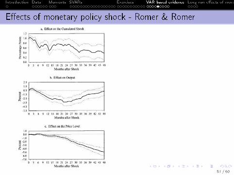
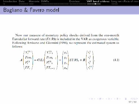
Bernanke & Mihov (1998, QJE) use a structural VAR (withAB decomposition) but include money market data and imposerestrictions only in this area (no macroeconomic restrictions)Romer & Romer (2004, AER) use a narrative approach - theystudy records from FOMC meetings. Find stronger and fastere�ects of monetary policy than those obtained usingconventional indicators.Bagliano & Favero (1999, EER), Gürkaynak, Sackb &Swanson (2005, IJCB), Gertler & Karadi (2012, AER): highfrequency identi�cation of shocks based on small time windowaround monetary policy decissions.Uhlig (2001), Canova & DeNicolo (2002, JME) use signrestrictions on impulse responses

48 / 60


Bernanke and Mihov restrictions

Impose a structural relationship between fedfunds rate, totalreserves and borowed reserves

49 / 60


E�ects of monetary policy shock - Bernanke & Mihov

50 / 60


E�ects of monetary policy shock - Romer & Romer

51 / 60


Bagliano & Favero model

52 / 60


E�ects of monetary policy shock - Bagliano & Favero

53 / 60


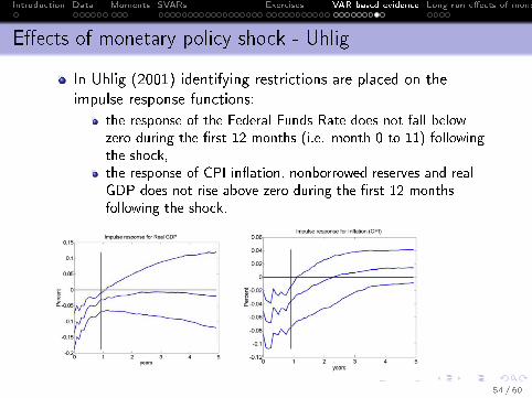
E�ects of monetary policy shock - Uhlig

In Uhlig (2001) identifying restrictions are placed on theimpulse response functions:

the response of the Federal Funds Rate does not fall belowzero during the �rst 12 months (i.e. month 0 to 11) followingthe shock,the response of CPI in�ation, nonborrowed reserves and realGDP does not rise above zero during the �rst 12 monthsfollowing the shock.

54 / 60


Conclusions based on VARs

After a contractionary monetary policy shock

output declinesmax reaction after a few (~3-5) quartersin�ation usually declines (reaction less clear)max reaction later than for outputsometimes price puzzle obtained (missing variables? - seeFAVAR Bernanke, Boivin, Eliasz 2005, QJE)

55 / 60



1 Introduction

2 Data

3 Moments

4 SVARs

5 Exercises



56 / 60


Neutrality of money (monetary policy)

Old concept (1930s)

Neutrality: money (monetary policy) does not in�uence realvariables

We already know: no neutrality in the short run

How about the long run?

Theory leans towards long-run neutrality (rational agentscannot be fooled permanently)With some exceptions:

very high in�ation destructive (resource allocation, othercosts)very low (negative) in�ation bad as well (DNWR)real money demand depends on nominal rates (see MIU)

Empirics?

57 / 60


Empirical literature

Empirical literature mildly in favor of long-run neutrality (King& Watson 1997, see Bullard 1999 for an overview)

King & Watson (1997) use US data 1949.1 - 1990.4

Estimate system with money and output

Result: long-run elasticity of output wrt money (γym) asfunction of identifying assumption on reverse elasticity (γmy )

58 / 60


Exceptions

Exceptions:

very high in�ation bad (Barro 1994)DNWR is an empirically con�rmed phenomenon (e.g. Lebow,Saks, Willson 2004)real money demand depends on nominal interest rates (Sriram2001 provides a survey)

59 / 60


Takeaways

To build good monetary models we need empirical evidence onmain (real and nominal) macro variablesThere is a lot of empirical evidence on business cycle behaviorbased on moments, e.g.:

consumption, investment are stronly and in�ation mildlyprocyclicalconsumption is less volatile than outputin�ation is persistent

We also have empirical evidence on the e�ects of monetarypolicy from VAR models

monetary contraction lowers output and in�ation (withsubstantial lags)

Finaly, we also have evidence on long-run e�ects of monetarypolicy

under normal conditions (no hyperin�ation, no persistentde�ation) monetary policy is neutral

60 / 60

Date post:	23-Mar-2022
Category:	Documents
Upload:	others
View:	7 times
Download:	0 times

Monetary economics Michaª Brzoza-Brzezina

Documents