Motorcycle Graph Enumeration from Quadrilateral …scad.itu.edu.tr/1/images/PDF3.pdfComputer Aided...

Computer Aided Design 00 (2016) 1–27

ComputerAidedDesign

Motorcycle Graph Enumeration from Quadrilateral Meshesfor Reverse Engineering

Erkan Gunpinar∗,1 Masaki Moriguchi2 Hiromasa Suzuki3 Yutaka Ohtake3

1Istanbul Technical University2Chuo University

3The University of Tokyo

Abstract

Recently proposed quad-meshing techniques allow the generation of high-quality semi-regular quadrilateral meshes. This paperoutlines the generation of quadrilateral segments using such meshes. Quadrilateral segments are advantageous in reverse engineer-ing because they do not require surface trimming or surface parameterization. The motorcycle graph algorithm of Eppstein et al.produces motorcycle graph of a given quadrilateral mesh consisting of quadrilateral segments. These graphs are preferable to basecomplexes, because the mesh can be represented with a smaller number of segments, as T-joints (where the intersection of twoneighboring segments does not involve the whole edge or vertex) are allowed in quadrilateral segmentation.

The proposed approach in this study enumerates all motorcycle graphs of a given quadrilateral mesh and optimum graph forreverse engineering is then selected. Due to the high computational cost of enumerating all these graphs, the mesh is cut intoseveral sub-meshes whose motorcycle graphs are enumerated separately. The optimum graph is then selected based on a costfunction that produces low values for graphs whose edges trace a large number of highly curved regions in the model. By applyingseveral successive enumeration steps for each sub-mesh, a motorcycle graph for the given mesh is found. We also outline a methodfor the extraction of feature curves (sets of highly curved edges) and their integration into the proposed algorithm. Quadrilateralsegments generated using the proposed techniques are validated by B-spline surfaces.

c© 2014 Published by Elsevier Ltd.

Keywords: Semi-regular quadrilateral mesh, Motorcycle graph, Mesh segmentation, Reverse engineering

1. Introduction

Recently developed quad-meshing techniques can be used to generate high-quality quadrilateral meshes based onuser-specified quality constraints. Such meshes are used in various applications such as mesh compression, texturemapping, surface modeling and finite element simulation. A quadrilateral mesh Q < V, E, F > consists of a set ofquadrilateral faces F with edges E and vertices V . Quadrilateral segments are defined on Q as quadrilateral regionswith four corners and four boundaries. In other words, they are isomorphic to an a, b-grid which is a mesh of unitsquares in the rectangle {(x, y)|0 ≤ x ≤ a, 0 ≤ y ≤ b}. In this paper, quadrilateral segmentation is used to describea partitioning of a quadrilateral mesh with quadrilateral segments. The left image of Fig. 1 (a) shows a quadrilateral

∗Corresponding author. Email address: [email protected], Address: Istanbul Technical University, Mechanical Engineering Faculty, InonuCaddesi, No: 65, Gumussuyu, 34437, Istanbul, TURKEY, Tel: +90-212-2931300, Fax: +90-212-2450795.

1

E. Gunpinar et al. / Computer Aided Design 00 (2016) 1–27 2

Figure 1: (a) A quadrilateral segment (right) has four boundaries (in red) and four corners (in blue) consisting ofregularly arranged quadrilateral faces. Quadrilateral segments in a quadrilateral mesh are illustrated in the left imagein (a). The computational cost of enumerating all motorcycle graphs that can be generated from a quadrilateral mesh(with 48 extraordinary vertices) of the Beetle model is very high. Accordingly, the mesh is cut into several sub-meshes(b) to reduce the time required. Enumeration is performed in each sub-mesh separately with successive steps, and aquasi-optimum graph (c) is obtained within about one second.

segmentation featuring several quadrilateral segments with boundaries in red and corners in blue. The right imagedepicts a quadrilateral segment consisting of regularly arranged quadrilateral faces.

Motorcycle graphs were first presented in continuous settings and can be used to compute straight skeletons ofpolygons [1, 2]. Later, Eppstein et al. [3] extended this concept to discrete settings (i.e., quadrilateral meshes) in orderto generate canonical quadrilateral segmentation (i.e., meshes with the same connectivity that always generate thesame quadrilateral segmentation). This paper highlights the concept of motorcycle graphs as a means of to generatingquadrilateral segments, and describes a novel algorithm that enumerates all motorcycle graphs of a given quadrilateralmesh so that one of them can be used for a specific application based on the criteria provided. In this approach, themethod of Bommes et al. [4] is used to generate a semi-regular quadrilateral mesh consisting of quadrilateral elementswhose vertices mostly have a valence of four (ordinary vertices), while the others have other valences (extraordinaryvertices).

This paper also outlines a methodology for the determination of an optimal motorcycle graph for a given quadri-lateral mesh to support reverse engineering. As the placement of highly-curved regions on quadrilateral segmentboundaries is a common practice in surface modelling applications, the cost formula introduced for optimum motor-cycle graph selection produces small values for motorcycle graphs whose edges trace a large number of highly curvedregions of the model. Additionally, feature curves (i.e., sets of highly curved edges) that are very difficult to capturewith motorcycle graph edges are also extracted and integrated into the enumeration algorithm. Because of high com-putational cost of the enumeration algorithm, a more efficient enumeration method (in terms of computational cost)is also proposed. Mesh is cut into several sub-meshes and optimal motorcycle graph in each sub-mesh is found. Byapplying successive enumeration steps, a motorcycle graph of a given mesh with proximity to the global optimum isobtained. Enumerating all motorcycle graphs of a Beetle model shown in Fig. 1 (b, c) takes several days according toour tests. Using the proposed approach in this paper, the enumeration takes about one second (see solution in Fig. 1(c)).

This paper is organized as follows: Section 2 outlines related works, Section 3 details the motorcycle graphenumeration algorithm, Section 4 describes a quadrilateral segmentation technique for reverse engineering based onthe enumeration algorithm in Sec. 3, Section 5 discusses the study’s experiments, and Section 6 concludes the work.

2. Related Works

The work reported here is related to quadrilateral meshing and mesh segmentation. Selected previous works arecovered in this section.

2.1. Quadrilateral Meshing

As the use of quadrilateral meshes is very common in a variety of computer graphics applications, quad-meshinghas been studied in detail for a number of years. Recently proposed state-of-the-art techniques can be used to produce

2


high-quality quadrilateral meshes whose elements are oriented according to principal curvature directions with goodelement quality such as square faces. Two review papers [5, 6] have detailed quad-meshing methods comprehensively.Early approaches [7, 8] define the quadrangulation problem based on the anisotropy of the given object. By tracinglines on the model using principal curvature directions, a quadrilateral mesh is generated from a triangular mesh.Rather than consisting of pure quadrilateral elements, the mesh generated also has triangular faces. The mixed-integerquadrangulation method [4] was motivated by the difficulty of defining principal curvature directions in spherical andflat parts as described in [7]. Accordingly, only certain principal curvature directions are utilized and are interpolatedall over the mesh. Quadrangulation is performed using these directions. Quadrilateral meshes generated using thismethod consist of only quadrilateral elements, most of which are non-degenerated. We also utilize quadrilateral meshgenerated using this method. Other recently proposed methods [9, 10, 11, 12, 13, 14, 15, 16, 17, 18, 19] can alsoapplied to produce pure triangle-free quadrilateral meshes using various techniques.

2.2. Quadrilateral Mesh Simplification

Recent works [20, 21, 22, 23, 24, 25, 26] have focused on structure optimization of quadrilateral meshes withthe aim of placing extraordinary vertices in appropriate positions to simplify the base complex of the mesh. Myles etal. [22] discussed the alignment problem for extraordinary vertices and simply updated the positions of extraordinaryvertices in the parametric domain, thereby achieving a simpler quadrilateral segment layout. In [23], the presenceof helical structures in the model is highlighted as a problem of extraordinary vertex alignment. These structuresstart from an extraordinary vertex, make several turns around the model and stop at extraordinary vertices, therebyproducing a not simple quadrilateral segment layout. They are removed by changing the local connectivity usingGrid-Preserving operators. In a very recent method proposed in [26], a dual layout is first constructed from curvature-guided crossing loops on the surface, and a quadrilateral mesh is then generated using this layout. The question ofhow the global structure of quadrilateral meshes can be simplified more remains an ongoing issue, and the proposalof new techniques is expected in the future.

2.3. Mesh Segmentation

Mesh segmentation has a long history in the graphics community, and numerous related literature surveys havebeen conducted [27, 28]. A wide variety of algorithms have been proposed for this problem, based on watershedanalysis [29, 30] hierarchical clustering [30], min-cut/max-flow [31], surface approximation [32], primitive-basedclustering [33, 34], fuzzy clustering and minimum cuts [35], surface construction [36, 37] and other approaches.Quadrilateral mesh segmentation algorithms are briefly discussed in the following sub-section.

2.3.1. Quadrilateral SegmentationUsing quadrilateral meshes for quadrilateral segmentation is easier than using arbitrary meshes because they have

well-arranged structures such that their elements are oriented according to the min/max curvature directions of themodel. Obtaining quadrilateral segmentation from these meshes is also trivial. However, the amount of work con-ducted on quadrilateral segmentation to date has been limited. The motorcycle graph algorithm of Eppstein et al. [3]segments a given quadrilateral mesh into quadrilateral segments whose extraordinary vertices are removed by placingthem on the boundary. Myles et al. [22] proposed a method for achieving quadrilateral segmentation from initialquadrilateral segmentation by changing the quadrilateral segment configuration using local operations. Gunpinar etal. [38] introduced bi-monotone (quasi-quadrilateral) segments that can capture feature curves that are not alignedwith parameter u-v directions, and therefore appropriate for B-spline surface fitting. Additionally, the feature-awarealgorithm [39] proposed by Gunpinar et al. generates quadrilateral segmentation using an approach in which pathsare greedily flipped to improve the initial path layout. Note that the approaches [20, 23, 21, 24, 25, 26] all producequadrilateral segments from a quadrilateral mesh. They are free from T-junctions different than the proposed methodin this paper and the methods [3, 22]. Once T-junctions are allowed, a smaller number of quadrilateral segments canrepresent the mesh which is important for reverse engineering applications. On the other hand, it causes the set ofpossible applications (such as subdivision surfaces) to shrink.

The objective of the method here is similar to those of the segmentation approaches outlined in [3, 22, 38, 39].As quadrilateral segmentation generated using the motorcycle graph algorithm [3] is canonical, the same motorcyclegraph is always generated from a given mesh. In the technique outlined here, numerous motorcycle graphs of a given

3


Figure 2: The base complex (a) of a given quadrilateral mesh is defined as the union of separatrices (in red) starting atan extraordinary vertex (in blue) and ending at an extraordinary vertex or a boundary vertex. Four different motorcyclegraphs (b) with boundaries (in red) generated from a given mesh.

mesh are enumerated, and one suitable for reverse engineering is selected. This method produces a better quadrilateralsegmentation than the motorcycle graph algorithm. With the approaches described in [22, 39], a quadrilateral segmen-tation is achieved by minimizing the values of the cost functions provided. In both approaches, the initial quadrilateralsegment layout is changed by greedily applying geometrical operators. As a result, several layout configurations areobtained and one of them is determined as the final configuration. These methods involve performing searches innarrow spaces due to the use of greedy techniques, and the solutions may converge to a local optimum. However, withthe algorithm proposed in this paper, a solution is sought in a rather wider space due to the enumeration techniqueused, and a better quadrilateral segmentation can thus be achieved. The drawback of the enumeration technique is thesignificant processing time involvement. For this reason, the mesh is cut into several sub-meshes and the enumerationalgorithm is applied to each one. In this step, the parameter χ introduced for the Mesh-Cut (as described in Section4.2.1) needs to be carefully adjusted. Otherwise, a large number of sub-meshes with narrow search spaces may beformed, and a solution far from the global optimum may be obtained. To capture feature curves that are not alignedwith parameter u-v directions, the use of bi-monotone segments [38] is much more advantageous than the use ofquadrilateral segments as adopted in [39] and the approach outlined in this paper. As the proposed technique involvesenumerating numerous motorcycle graphs for a given quadrilateral mesh, it results in a better quadrilateral segmenta-tion (where more highly-curved regions are placed on quadrilateral segment boundaries) than approaches [38, 39], inwhich greedy techniques are used for the same purpose.

3. Enumeration of Motorcycle Graphs on Quadrilateral Meshes

3.1. Base Complex vs. Motorcycle Graph

In the approach by Eppstein et al. [3], edges are traced on a quadrilateral mesh Q by moving particles to generatetracks. The particles are placed on extraordinary vertices and moved outward from these vertices along one edge oneby one. When a particle reaches an ordinary vertex, it continues to move straight along its opposite edge. Particles stopwhen they reach extraordinary vertices or at the mesh boundary, and the edges they trace generate tracks on Q. Suchtracks form separatrices, and their union is known as a base complex (Fig. 2 (a), red). For meshes without boundaries,a particle starting at an extraordinary vertex v1 ends at another extraordinary vertex v2, while one starting at v2 endsat v1. These two particles trace two separatrices between v1 and v2 in opposite directions. Note that separatrices aredirected in this work.

The following rules are added to the above particle tracing for motorcycle graph generation [3]: Particles stop ifthey meet already traced vertices. When two particles meet simultaneously at a vertex, the particle clockwise fromthe right angle formed by the tracks of two particles stops, while the other one keeps going.

The tracks generate quadrilateral segments under these rules. The graph structure of such segments is known asmotorcycle graph as proposed by Eppstein et al. [3]. These graphs have different topological structures to those ofbase complexes. T-joints can be seen in motorcycle graphs such that the intersection of two neighboring segments isnot the whole edge or vertex. Allowing T-joints in this way makes it possible to represent the mesh with a smallernumber of segments.

4


3.2. Notations and DefinitionsThe notations described here are based on a quadrilateral mesh that is homeomorphic to a two-manifold without

a boundary. Figure 3 shows two separatrices and their local coordinate systems with notations. Here let the i-thseparatrix in a base complex be called S i (in blue). The vertex on S i whose local coordinate on S i is j is denoted asvertex(S i, j), and opp(S i) (in red) is the index of the opposite separatrix of S i. left(S i, j) (in green) and right(S i, j) (inlight blue) are the indices of the left and right separatrices of S i at vertex(S i, j) which should be an internal vertex ofS i. The local coordinate on S i of vertex v is denoted as coordi(v), where v is a vertex of S i. length(S i) is the length ofS i which is the total number of vertices in S i minus one.

The 1D local coordinate system for the separatrix S i is based on the notations provided, and the position (coordi-nate) of a particle on S i is represented by the integer xi. The initial endpoint of the separatrix S i has the coordinate0 in the coordinate system of S i, and its terminal endpoint has the coordinate length(S i). The coordinate value of apoint increases by one when it moves to the next vertex away from the origin.

Suppose the input base complex has n separatrices, and a particle is placed on each one. Let the i-th particle becalled as pi which starts at the initial endpoint of the separatrix S i and moves along S i until it is stopped. The point atwhich a particle stops is called the crashing point. The crashing point of pi is denoted as κi. The track of pi, denotedas Ti, is the path on S i starting at the initial endpoint of S i and ending at the crashing point κi. If each particle track Ti

satisfies the following conditions, the set of particle tracks {Ti}ni=1 is considered valid:

A1. (No overlapping tracks.) xi ≤ length(S i) − xopp(S i) .

A2. (No crossing tracks.) For each internal vertex v of Ti, xleft(S i, j) ≤ coordleft(S i, j)(v) and xright(S i, j) ≤ coordright(S i, j)(v) ,where j = coordi(v).

A3. (No inactive particles.) If xi = 0, then xopp(S i) = length(S i) .

A4. (No dangling tracks, no L-junctions.) If 0 < xi < length(S i) − xopp(S i), then one of the following holds ( j = xi).

(1) xopp(S i) = length(S i) − xi .

(2) xopp(S i) < length(S i) − xi and xleft(S i, j) ≥ coordleft(S i, j)(κi) + 1 .

(3) xopp(S i) < length(S i) − xi and xright(S i, j) ≥ coordright(S i, j)(κi) + 1 .

(4) xopp(S i) < length(S i) − xi , xleft(S i, j) = coordleft(S i, j)(κi) and xright(S i, j) = coordright(S i, j)(κi) .

Otherwise the set is considered invalid. Figure 4 shows the five types of invalid particle tracks. A graph formed byvalid particle tracks is called a motorcycle graph, and induces quadrilateral segmentation with T-junctions. Differentparticle tracks can form the same motorcycle graph as seen in Fig. 5. Note that, if a base complex has a separatrixwith self-crossing (self-intersection at an internal vertex of a separatrix), invalid motorcycle tracks can be generated.To avoid such cases, these separatrices should be detected and truncated to the intersection vertex.

3.3. Motorcycle Graph Enumeration AlgorithmLet particles move at different speeds. The order of arrival at vertices changes, and thus the resulting motorcycle

graphs also change. Figure 2 (b) shows four different motorcycle graphs generated from the same quadrilateral mesh(a), all of which are structured. All of these graphs can be enumerated so that the optimum one for some criterion canbe selected from them. As particle tracks determine this graph, particles need to be placed in appropriate positions toprevent invalid results such as non-motorcycle graphs. These positions must be at the vertices of the base complex.

Let the input base complex have n separatrices. As motorcycle graphs are formed by valid tracks that can berepresented by the local coordinates of their crashing points, they can be enumerated by enumerating the coordinatesx1, . . . , xn. A naive method for enumerating valid tracks is to first enumerate all coordinate combinations and thenfilter out invalid tracks. This enumeration can be performed using a simple recursive procedure:

EnumerateCoordinates(Q) /* Q: a base complex with n separatrices. */

5


Figure 3: (a) Two separatrices (S i and S opp(S i)) and their local coordinate systems. The separatrix S i shown in blue, theopposite separatrix S opp(S i) of S i in red, the left separatrix (at j = 2) S left(S i,2) of S i in green, and the right separatrix (atj = 2) S right(S i,2) of S i in light blue. Symbols used in the figures: (b) Irregular vertex (c) Regular vertex (d) Undirectedseparatrix (e) Separatrix (f) Particle track (Arrow tip: crashing point) (g) Particle track (Crashing point not shown)

Figure 4: Invalid particle tracks: (a) Overlapping (b) Crossing (c) Inactive particle (d) Dangling track (e) L-junction

Figure 5: Different particle tracks with the same motorcycle graph.

6


1: Call Enumerate(1, n).

Enumerate(i, n) /* Recursively enumerate coordinates xi, . . . , xn. */

1: if i ≤ n then2: for j = 0, . . . , length(S i) do3: Set xi to j.4: Call Enumerate(i + 1, n) recursively.5: else6: if the coordinates x1, . . . , xn represent valid tracks then7: Output x1, . . . , xn

However, this naive method is inefficient because a large number of invalid tracks are unnecessarily enumeratedbefore being eventually filtered out. The next section describes a method for avoiding such inefficiency.

3.3.1. Enumeration without Invalid TracksTo efficiently enumerate motorcycle graphs, it is important to avoid invalid tracks. This is achieved by main-

taining lower and upper bounds of coordinates to enforce validity conditions (A1)–(A4). The basic structure of thisenumeration is same as that of the naive method, and a recursive procedure is used to enumerate the coordinates.The difference is that the lower and upper bounds of the coordinates are maintained, and these bounds are used toprevent unnecessary enumeration. Let Li and Ui denote the lower and upper bounds of coordinate xi, respectively.The modified version of EnumerateCoordinates is as follows:

EnumerateCoordinates(Q) /* Q: a base complex with n separatrices. */

1: // Initialize lower bounds . ”//” = Comment line2: Set Li to 0, for i = 1, . . . , n.3: // Initialize upper bounds4: Set Ui to length(S i), for i = 1, . . . , n.5: Call Enumerate(1, n).

To enforce the validity conditions, the lower and upper bounds are updated in the following way, which is simplyderived from (A1)–(A4):

B1. (Preventing overlapping tracks.) Suppose coordinate xi is set to j. The upper bound Uopp(S i) is updated tolength(S i) − j.

B2. (Preventing crossing tracks). Suppose coordinate xi is set to j. For k = 1, . . . , j− 1 , Ul is updated to coordl(v)and Ur to coordr(v), where v = vertex(S i, k), l = left(S i, k) and r = right(S i, k).

B3. (Preventing inactive particles.) Suppose the coordinate xi is set to 0. The lower bound Lopp(S i) is updated tolength(S i).

B4. (Preventing dangling tracks and L-junctions). Suppose the coordinate xi is set to j (0 < j < length(S i)). Letv = vertex(S i, j), l = left(S i, j) and r = right(S i, j). There are four cases.

(1) Both Lopp(S i) and Uopp(S i) are updated to length(S i) − j.

(2) Uopp(S i) is updated to length(S i) − j − 1. Ll is updated to coordl(v) + 1.

(3) Uopp(S i) is updated to length(S i) − j − 1. Lr is updated to coordr(v) + 1.

(4) Uopp(S i) is updated to length(S i) − j − 1. Both Ll and Ul are updated to coordl(v), and both Lr and Ur areupdated to coordr(v).

7


Note that any one of (B4-1), (B4-2), (B4-3) and (B4-4) guarantees the prevention of dangling tracks and L-junctions,and each of them generates a different set of tracks.

Modified version of Enumerate(i, n) is written in the below. The cases of xi = 0 and xi = length(S i) are excludedfrom the for-loop iteration because the track Ti can neither be a dangling track nor have an L-junction. For sake ofsimplicity, these cases are not shown in the below pseudo code. The bounds are updated according to (B3) for xi = 0and according to (B1) and (B2) for xi = length(S i). In the loop body, the update methods of (B1) and (B2) are firstapplied, and the bounds are then updated. A recursive call is made to Enumerate(i+1, n) using each of (B4-1), (B4-2),(B4-3) and (B4-4), therefore the loop body has four enumeration branches. In the pseudo code, ς refers to the set oflower and upper bounds {Li,Ui}

ni=1 for particles, and the values for these sets are denoted as ψt, where t = 0, 1, ..., 5.

Enumerate(i, n) /* Recursively enumerate coordinates xi, . . . , xn. */

1: if i ≤ n then2: for j = Li, . . . ,Ui do3: Set xi to j (ς = ψ5).4: Update the lower and upper bounds (LU bounds) using the (B1) and (B2) rules (ς = ψ0).5: // Case (B4-1)6: Update the LU bounds using the (B4-1) rule (ς = ψ1).7: Call Enumerate(i + 1, n) recursively.8: Restore the LU bound values before Line 6 (ς = ψ0).9: // Case (B4-2)

10: Update the LU bounds using the (B4-2) rule (ς = ψ2).11: Call Enumerate(i + 1, n) recursively.12: Restore the LU bound values before Line 10 (ς = ψ0).13: // Case (B4-3)14: Update the LU bounds using the (B4-3) rule (ς = ψ3).15: Call Enumerate(i + 1, n) recursively.16: Restore the LU bound values before Line 14 (ς = ψ0).17: // Case (B4-4)18: Update the LU bounds using the (B4-4) rule (ς = ψ4).19: Call Enumerate(i + 1, n) recursively.20: Restore the LU bound values before Line 18 (ς = ψ0).21: Restore the LU bound values before Line 4 (ς = ψ5).22: else23: Output x1, . . . , xn

The lower and upper bounds are said to be consistent when each lower bound is lower than or equal to thecorresponding upper bound. If the bounds are not consistent, there are no valid tracks in that enumeration branch.Whenever bounds are updated, consistency is checked; if the check fails, enumeration is stopped for that branch.Maintaining the lower and upper bounds requires some care. When the coordinate xi is set to j, Li and Ui are alsoset to j to facilitate bound consistency checking. If the new bound is weaker than the old one after updating, the oldone is kept. Restoring a bound means setting it back to the old one (i.e., that before the update). To efficiently supportupdate and restore operations, stacks are used to represent bounds.

3.3.2. Improved AlgorithmThe previous algorithm succeeds in (duplication-free) enumeration of particle tracks without invalid ones. How-

ever, the algorithm is still inefficient from the viewpoint of motorcycle graph enumeration: it generates duplicatemotorcycle graphs, as different particle tracks can form the same motorcycle graph (Fig. 5). To improve the effi-ciency, duplications are reduced by avoiding enumeration of particle tracks with a certain property. Note that, sinceour application does not require duplication-free enumeration, we do not aim to remove duplications completely.

Suppose a pair of opposite particles pi and popp(S i) collide and stop at the same vertex v. If v is an internal vertex ofseparatrix S i, we call it a crack between tracks Ti and Topp(S i). In Fig. 5 (a–c), there is a crack between the horizontaltracks. But, in Fig. 5 (d–e), since the common crashing point of the two particles on the horizontal separatrices is notan internal vertex of the separatrix, there is no crack. Suppose there is a crack between Ti and Topp(S i), and let j be

8


Figure 6: (a) Penetrated crack (b-d) Non-penetrated cracks.

Figure 7: Quadrilateral mesh model of a torus (a) generated by gluing parallel sides of a rectangle (b)

the local coordinate of the crack on S i. If particle pleft(S i, j) (or pright(S i, j)) goes beyond the crack, the crack is calledpenetrated; otherwise it is called non-penetrated. Fig. 6 shows penetrated and non-penetrated cracks.

Let T1, . . . ,Tn be valid tracks. Suppose there is a non-penetrated crack between tracks Ti and Topp(S i). By changingthe position of the common crashing point of particles pi and popp(S i) to an endpoint of S i (i.e. setting xi = 0 andxopp(S i) = length(S i), or xi = length(S i) and xopp(S i) = 0), the crack between Ti and Topp(S i) can be removed. Thevalidity of the tracks and the motorcycle graph formed by them are not changed by this operation. All non-penetratedcracks can be removed by repeated application of the operation, and the motorcycle graph does not change during thisprocess. This indicates that, for any valid tracks that have non-penetrated cracks, there exist valid tracks that have thesame motorcycle graph and that do not have non-penetrated cracks.

Thus, for motorcycle graph enumeration, it is not necessary to enumerate tracks that have non-penetrated cracks.To skip enumeration of these tracks, the update rule (B4) is modified as follows:

B4′. (Preventing dangling tracks and L-junctions). Suppose the coordinate xi is set to j (0 < j < length(S i)). Letv = vertex(S i, j), l = left(S i, j) and r = right(S i, j). There are two cases.

(1) Ll is updated to coordl(v) + 1.

(2) Lr is updated to coordr(v) + 1.

Our improved algorithm uses (B1), (B2), (B3) and (B4′).The speed-up achieved using the Improved Algorithm (in Section 3.3.2) is quantified for a torus model as shown in

Figure 7 (a), whose base complex has 68 vertices, 68 quadrilateral faces and 32 undirected separatrices. Computationfor this model takes 1525.2 seconds using the enumeration algorithm described in Section 3.3.1 and just 44.467seconds with the Improved Algorithm. These times were measured on a PC with an Intel Core i7 2.6 GHz processor16 GB of memory using single-threaded implementation.

4. Quadrilateral Segmentation for Reverse Engineering

The objective of the algortihm described in this section is to find the optimal motorcycle graph for reverse engi-neering by enumerating all motorcycle graphs of a given quadrilateral mesh. Due to the high computational cost of

9


the enumeration algorithm outlined in Section 3, a more efficient enumeration method is proposed in Section 4.2. Thecost formula introduced in Section 4.1 includes a criterion (capture of features) for the segments, which is a commonpractice in surface modelling applications: Segment boundaries should pass through feature regions (such as highlycurved parts) of the mesh. Section 4.3 outlines a method for the extraction of feature curves (sets of highly curvededges) and their integration into the proposed algorithm.

4.1. Cost Function for Reverse Engineering:

Various cost functions can be introduced for use in the selection of optimum quadrilateral segmentation appropriatefor reverse engineering applications. A cost formula is chosen which is the same as that of Gunpinar et al.’s work [39].This formula produces small values for graphs whose edges trace a large number of highly curved regions of the model,and therefore favors placing highly curved edges in the mesh to the segment boundaries as many as possible.

A set of quadrilateral segments can be obtained from a set of particle tracks ({Ti}). The unsigned dihedral angleθ(e), (0 ≤ θ(e) ≤ π) of the edge e is the angle between the normal vectors of its adjacent faces. Normal vector for aquadrilateral face is computed by averaging normal vectors of its two triangles. θ(e) is 0 for a flat edge with two flatfaces, and shows large values for sharp edges. In this study, dihedral angle is chosen as a geometric criterion becauseof its low computation cost.

The cost function F(Ti) of the particle track Ti is defined to give a low-cost value for a particle track of edgeswith large dihedral angles. F(Ti) is defined as F(Ti) = −C(Ti) + αD(Ti). C(Ti) =

∑e j∈Ti

θ(e j) is simply the sum ofall dihedral angles for the edges of Ti and D(Ti) =

∑e j∈Ti

d(e j), where d(e j) is 0 if θ(e j) ≥ ε, and is 1. The parameterε is set to 1.0 for the drill hole and bottle models, and to 0.2 for the Beetle and rockerarm models. According toour experience, fine-tuning of this parameter results in the generation of similar quadrilateral segmentations. D(Ti)is introduced because particle tracks that are less curved and longer have a lower cost without it. Such tracks aretherefore not desirable. A set of particle tracks {Ti} that minimizes the global cost GT =

∑i F(Ti) is sought. α can be

set to 1 in order to assign equal weights to the terms C(Ti) and D(Ti). However, it is set to 0.4 to give greater weightto the term C(Ti), as tracing of highly-curved regions in the model is favored.

4.2. Cut-and-Merge Based Enumeration

Suppose there are n particles each with c candidate positions, and naive method described in Section 3.3 enu-merates cn number of particle positions. For the motorcycle graph enumeration, this number will be smaller becausemotorcycle graphs are restricted. However, as the number is still exponential, the enumeration has high computationalcost, particularly with meshes for which the base complex is not simple. To simplify the motorcycle graph enumer-ation problem and speed up its resolution, our main approach involves dividing a given mesh into sub-meshes toallow separate enumeration of their motorcycle graphs, and then selecting optimum graphs for each sub-mesh. Thesemotorcycle graphs are then merged to generate one for the whole mesh. Figure 15 shows base complexes (a, c) of adrill hole model. After the mesh is cut into sub-meshes, 8 sub-meshes are generated from the initial model. The totalnumber of ordinary junctions is reduced to 45 from 1344.

With a mesh cut into sub-meshes, it is obvious that the optimum motorcycle graph of the mesh may not be found.If the absolute optimum solution is needed, the enumeration algorithm should be directly applied without applyingCut-and-Merge based enumeration, which has high computational cost. However, based on the outcomes of thisstudy’s experiments, the motorcycle graphs generated with the Cut-and-Merge based enumeration are suitable forreverse engineering and they can be considered to approximate a global solution.

4.2.1. Mesh-Cut Algorithm with Graph-CutIn this step, sub-meshes with simpler underlying base complexes are generated from a given quadrilateral mesh

using the minimum cut algorithm of Boykov et al. [31], and any separatrices with helical structures are also eliminated.A weighted graph G < V, E > is constructed using vertex and edge elements of the quadrilateral mesh Q < V, E, F >,where undirected edges in E connect the set of nodes in V . The terminals source and sink, which are two differentvertices in V , are first found, and the minimum cut separating these terminals is then computed. The cut divides themesh Q into two sub-meshes. In order to avoid generation of short cuts where one sub-mesh is large and the other isvery small, the energy function is designed based on Golovinskiy et al.’s work [40], which favors the generation of

10


Figure 8: Total number of ordinary junctions in base complexes (separatrices in various colors): (a) without cut: 4574.(b) with cut (in red): 1304. (c) with cut: 426. The positions of source (green sphere) and sink (blue sphere) terminalstherefore affect the base complex complexity of sub-meshes obtained using the graph-cut method.

Figure 9: (a) Distribution of irregular vertices (in red) in the mesh boundaries in black (mesh edges, faces and ordinaryvertices are not shown) is taken into account for the computation of source s and sink t terminals. (b) After the irregularvertex pair p1 − p2 with the maximum distance apart is found, all irregular vertices are grouped into two by checkingproximity to p1 and p2. The vertices closest to the group centers are selected as source and sink. (c) Irregular vertexdistribution and computed source-sink vertices (green-blue spheres) are shown for the drill hole model.

sub-meshes with largely similar areas. This algorithm is applied repeatedly until sub-meshes with the desired level ofbase complex simplicity are obtained.

Selection of Terminals: To generate sub-meshes with well-simplified base complexes, source and sink vertices ofa cut should be appropriately selected. The basic idea behind such selection is to enable the separation of extraordinaryvertices in a given mesh (or sub-mesh) as equally as possible by finding appropriate positions for the source and sinkbecause the complexity of a base complex is related to the locations and number of these extraordinary vertices, atwhich the separatrices of a base complex start and end. Accordingly, cutting is desirable if the resulting sub-meshescontain almost equal numbers of extraordinary vertices. Figure 8 shows base complexes with separatrices depicted invarious colors. Two different cuts (in red) are obtained for different settings of the source (green sphere) and sink (bluesphere) terminals. The base complexes of sub-meshes in the latter (c) are much simplifier than those in the former (b)such that the total number of ordinary junctions in the base complexes is further reduced.

Irregular vertices in the mesh are used to compute the source and sink terminals. The irregular vertex pair p1 − p2(see Fig. 9) furthest apart is first found by checking distances between all irregular vertices (in red) in the mesh(boundaries in black). All irregular vertices are then grouped into two according to their distances to p1 and p2.Geodesic distance is used for these computations. Finally, the center of the two groups is calculated and the two meshvertices closest to it are assigned as the source and sink terminals. Figure 9 shows source (green sphere) and sink(blue sphere) vertices computed using this approach, which enables almost-equal separation of irregular vertices andproduces a simpler base complex after cutting.

Energy Function: The two-terminal graph constructed is segmented into two sub-graphs by finding a cut that

11


minimizes the following energy function:

E(L) =∑p∈V

Gp(Lp) + λ∑

(p,q)∈N

f (Lp, Lq),

where λ is to set to 1 to assign equal weights to the terms Gp(Lp) and f (Lp, Lq), and fine-tuning of the parameter λgenerates the similar cuts according to our experience. L =

{Lp|p ∈ V

}is a labeling of the mesh vertices V where

Lp ∈ {S ,T } denotes a label given to a vertex. If the vertex p is assigned to the source terminal side, Lp = S . Otherwise,Lp = T . Gp(Lp) is a data penalty function and f (Lp, Lq) reflects the interaction potential between all pairs of 1-ringneighboring vertices where N represents a set of all of these pairs. f (Lp, Lq) is set to 1 if Lp , Lq; otherwise, it is 0.

From each vertex in V to both the source and sink terminals, a penalty cost Gp(Lp) is assigned as follows:

Gp(Lp) =

Wh if D(Lp, p) ≤ m1;

Wl + ν(m2 − D(Lp, p)) if m1 < D(LP, p) ≤ m2;Wl if D(Lp, p) > m2.

where D(LP, p) = 1 − (dst(LP, p)/(dst(S , p) + dst(T, p))) varying between 0 and 1, and ν = (Wh − Wl)/(m2 − m1).dst(LP, p) is the geodesic distance between vertex p and the source terminal when LP = S or the sink terminal whenLP = T . This formula favors cutting that is not very close to either of the source or sink terminals. In this way, shortcuts are avoided and cuts that are equi-distant from terminals are promoted. In this study, the coefficients are set toWh = 80, Wl = 1, m1 = 0.4 and m2 = 0.5. It is recommended to set m2 to 0.5 which favors cuts that are equi-distantfrom terminals, and if D(Lp, p) ≤ 0.4, it is penalized with a high-cost Wh. The authors have found that fine-tuning ofthe parameters Wh, Wl, m1 and m2 results in the generation of similar cuts.

To favor equal separation of extraordinary vertices, penalties are imposed on such vertices when they are notassigned to their previously determined terminal group (see ”Selection of Terminals”). Recall that extraordinaryvertices are classified into two groups shown with encircled ellipses in Fig. 9 (b) (the source group in light green andthe sink group in light blue). For an extraordinary vertex previously determined to be the source (or sink) group, thevalue D(vLP , p) is updated as 1 so that separation of this vertex from the source (or sink) group is penalized.

Number of Cuts: The previously explained graph cut algorithm segments a given mesh into two sub-meshes.The base complexes of these sub-meshes are computed separately to be much simpler than that of the initial mesh,and the number junctions where separatrices meet is thus drastically reduced. However, cutting the mesh only once isnot generally enough to obtain the desired level of base complex simplicity. In such cases, it is necessary to apply thegraph cut algorithm several times until all sub-meshes obtained have the desired level of base complex simplicity.

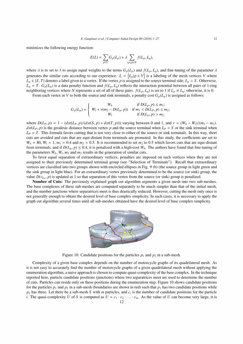
Figure 10: Candidate positions for the particles p1 and p2 in a sub-mesh.

Complexity of a given base complex depends on the number of motorcycle graphs of its quadrilateral mesh. Asit is not easy to accurately find the number of motorcycle graphs of a given quadrilateral mesh without applying theenumeration algorithm, a naive approach is chosen to compute quasi-complexity of the base complex. In the techniquereported here, particle candidate positions (junctions) where two separatrices meet are used to determine the numberof cuts. Particles can reside only on these positions during the enumeration step. Figure 10 shows candidate positionsfor the particles p1 and p2 in a sub-mesh (boundaries are shown in red) such that p1 has two candidate positions whilep2 has three. Let there be a sub-mesh S with m particles, and ci is the number of candidate positions for the particlei. The quasi-complexity U of S is computed as U = c1 · c2 · . . . · cm. As the value of U can become very large, it is

12


simplified using a logarithm such that U = log2 c1 + log2 c2 + . . . + log2 cm. The U value of each sub-mesh shouldbe smaller than the parameter χ, otherwise the sub-meshes will be segmented into two using the graph-cut algorithmuntil sub-meshes with U values smaller than χ are obtained. It is recommended to set χ parameter between 20 and 60which is assigned as 20, 40 and 60 during experiments. Otherwise, processing may take a large amount of time. It isobserved that fine-tuning of the χ parameter does not affect the results.

Results: Figure 11 shows cuts generated (boundaries shown in various colors) for different test models withplaced particles in red. The total number of ordinary junctions (n j) in the base complexes and the number of sub-meshes (nG) before (Original) and after (χ = 40, 20) applying the Mesh Cut algorithm are detailed in Table 1. Thenumber of ordinary junctions drastically decreases after applying the proposed cut algorithm, and this number fallseven further for smaller χ values so that base complexes become less complex. It should be noted that the drill holeand rockerarm models have a high number of ordinary junctions in their initial base complexes due to the presenceof helical structures as shown in Fig. 15. Cutting the mesh into two sub-meshes eliminates the complexity resultingfrom these structures.

Original χ = 40 χ = 20Models n j nG n j nG n j

drill hole 1344 5 73 8 45Beetle 199 5 94 8 52bottle 623 6 71 8 52

rockerarm 4574 8 109 12 66

Table 1: Number of ordinary junctions (n j) in base complexes and number of sub-meshes (nG) before (original) andafter the Mesh-Cut algorithm.

Figure 11: Cuts generated (boundaries in various colors) with different test models for χ = 20 and χ = 40. Particlesplaced are shown in red.

4.2.2. Extended Enumeration AlgorithmThe enumeration algorithm detailed in Section 3 works for a quadrilateral mesh homeomorphic to a two-manifold

without boundary. A sub-mesh may have two types of boundary after applying the Mesh-Cut algorithm: Meshboundary (like in the Beetle model) or Cut boundary (see cuts in Figure 11). The Mesh-Cut algorithm separates thevertices in the mesh into two groups and the generated cuts may pass through some faces which will not be assignedas the elements of two generated sub-meshes. Let o sub-meshes B1, B2, ..., Bo are generated after cutting. A sub-meshBi has the vertices Vi ⊂ V , the edges Ei ⊂ E and the faces Fi ⊂ F where V1∪V2∪ . . .∪Vo = V , E1∪E2∪ . . .∪Eo , Eand F1 ∪ F2 ∪ . . . ∪ Fo , F. Neighboring vertices of Bi are the vertices in 1-ring neighborhood that are elements of

13


Figure 12: (a) The base complex of the sub-mesh S A is computed. Particles are stopped after passing cuts (in red).(b) Motorcycle graph enumeration is performed. Some particles (called as free particles) go beyond the cut and somestop (tracks marked with black and blue circles, respectively) (c) Free particles (tracks marked with red circles) in S A

are taken into account during base complex computation of the sub-mesh S B. (d) Particle positions after the graphenumeration in S B (tracks of free particles thickened)

another sub-mesh B j ( j , i). Note that a vertex on the boundary is an extraordinary vertex whose valence is at leastfour.

While computing base complex of a sub-mesh, separatrices are formed that start from extraordinary vertices andcan end at extraordinary vertices, Mesh boundary vertices or neighboring vertices. Motorcycle graph enumeration fora sub-mesh is performed to obtain particle tracks using its base complex in a similar way explained in Section 3 andthe particle candidate positions can be intersection vertices of separatrices, extraordinary vertices, Mesh boundaryvertices or neighboring vertices. Motorcycle graph of a sub-mesh is the union of the obtained particle tracks afterthe enumeration. However, some separatrices in a sub-mesh may not have their opposite, left or right separatrices.Accordingly, the update rules (B1), (B2), (B3) and (B4′) should be customized for these separatrices (not for others).

B1. (Preventing overlapping tracks.) Suppose the coordinate xi is set to j. No need to update Lopp(S i) if theseparatrix S i does not have opposite separatrix (opp(S i)).

B2. (Preventing crossing tracks). Suppose the coordinate xi is set to j. For k = 1, . . . , j−1 , no need to update Ul ifthe separatrix S i does not have left(S i, k), where v = vertex(S i, k), l = left(S i, k) and r = right(S i, k). Similarly,no need to update Ur if the separatrix S i does not have right(S i, k).

B3. (Preventing inactive particles.) No recursive call needed if the separatrix S i does not have opposite separatrix.

B4′. (Preventing dangling tracks and L-junctions). Suppose the coordinate xi is set to j (0 < j < length(S i)). Letv = vertex(S i, j), l = left(S i, j) and r = right(S i, j).

(1) No recursive call needed for the separatrix S i with no left(S i, k).

(2) No recursive call needed for the separatrix S i with no right(S i, k).

4.2.3. Merging Motorcycle GraphsMotorcycle graphs of the obtained sub-meshes are enumerated using the Partial MC Generator and the Complete

MC Generator and finally a graph representing a motorcycle graph for the whole mesh is obtained. Selection of theoptimum graph for each sub-mesh is based on a cost function which will be also described here.

Partial MC Generator (PMG): The main aim here is to find the optimum motorcycle graph for each sub-meshby applying the enumeration algorithm in Section 3. After the enumeration, the optimum graph is selected, and someparticles in this graph go beyond the cut which are called as free particles while others stop inside the sub-mesh.Figure 12 shows the cuts (in red) and enumeration for the sub-meshes S A and S B. The tracks of free particles aremarked with black circles (b) and are thickened, and the tracks of others are marked with blue circles (b). For the nextenumeration performed in another sub-mesh, free particles are also used in base complex computation. Namely, freeparticles of S A (b) are also taken into account when the base complex of S B is computed (marked with red circles (c)).In this way, particles with dangling tracks go further and stop (d).

Complete MC Generator (CMG): The union of optimum graphs after applying PMG may not represent a motor-cycle graph when the whole mesh is considered. Therefore, CMG is implemented to perform successive enumeration

14


Figure 13: A motorcycle graph in a sub-mesh (boundaries shown in red) is shown (a) with a free particle (track shownin light green). To assign a position for this particle, enumeration in the sub-mesh is required. The base complex iscomputed (b) using only certain particles (tracks shown with dashed lines), and other particles (tracks shown withsolid lines) do not need to be considered during graph enumeration. Candidate positions are depicted with black dots.(c) After applying the PMG, a motorcycle graph for the whole mesh is generated where no free particles are left.

steps in sub-meshes separately until a motorcycle graph for the whole mesh is obtained. The same methodology asthat for the PMG is used for the CMG, but only certain particles are considered during the enumeration step. Theseare free particles and linked particles, which are those to be included in the enumeration with free particles to avoidthe generation of invalid motorcycle tracks. In Figure 13 (b), particles with tracks shown in orange, pink, purple, grayand blue colors are linked particles.

Figure 13 (a) shows an invalid motorcycle graph consisting of particle tracks. The particle track shown in lightgreen is that of a free particle which should be positioned after performing enumeration in the sub-mesh (boundariesshown in red). The base complex is computed using this free particle and related particles, whose separatrices tracedare shown with dashed lines (b). The particle candidate positions that are used for the enumeration are marked withblack dots. The tracks of other particles (tracks marked with solid lines) do not need to be considered during theenumeration process. Starting with such a base complex, enumeration is performed and the optimum motorcyclegraph is selected from among those enumerated. Figure 13 (c) shows the motorcycle graph generated after severalsuccessive enumeration steps. As mentioned in the previous paragraph, such successive steps are performed until amotorcycle graph for the whole mesh is obtained. It should be noted that the CMG may not always converge to avalid motorcycle graph for the whole mesh; that is free particles may always be present after enumerations. However,no such cases were observed in the experiments of this study. To overcome this convergence problem, various naiveapproaches can be proposed. After detecting repetitive segment configurations causing unconvergence, free particlesin each configuration are extended to obtain motorcycle graph for the whole mesh. Optimum motorcycle graph canthen be chosen.

4.3. Integration of Feature CurvesExtraordinary vertices are not always connected to or near the highly curved regions. As a result, these regions

inevitably reside inside the generated quadrilateral segments of motorcycle graph. For reverse engineering applica-tions such as surface modeling, it is crucial to locate as many such regions as possible on segment boundaries. Afterthe highly-curved regions that are very difficult to capture with the particles placed on extraordinary vertices havebeen detected and extracted, and additional particles are placed on these curves to enable them to be traced. Theseparticles are then integrated to the motorcycle graph enumeration algorithm in the same way as particles located onextraordinary vertices.

The highly-curved regions mentioned above are called as feature curves, and have three main properties:

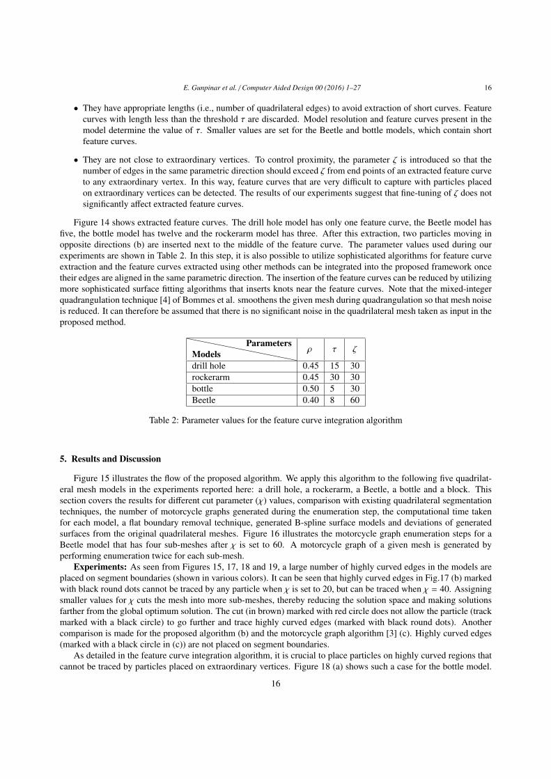
• They are sets of highly curved connected edges in the same parametric direction. In other words, all theseconnected edges have dihedral angles (in radian) greater than the flatness threshold ρ. Setting ρ to smallervalues results in the generation of numerous feature curves, which may be undesirable. The value is thereforeset between 0.4 and 0.5 in the study’s experiments.

15


• They have appropriate lengths (i.e., number of quadrilateral edges) to avoid extraction of short curves. Featurecurves with length less than the threshold τ are discarded. Model resolution and feature curves present in themodel determine the value of τ. Smaller values are set for the Beetle and bottle models, which contain shortfeature curves.

• They are not close to extraordinary vertices. To control proximity, the parameter ζ is introduced so that thenumber of edges in the same parametric direction should exceed ζ from end points of an extracted feature curveto any extraordinary vertex. In this way, feature curves that are very difficult to capture with particles placedon extraordinary vertices can be detected. The results of our experiments suggest that fine-tuning of ζ does notsignificantly affect extracted feature curves.

Figure 14 shows extracted feature curves. The drill hole model has only one feature curve, the Beetle model hasfive, the bottle model has twelve and the rockerarm model has three. After this extraction, two particles moving inopposite directions (b) are inserted next to the middle of the feature curve. The parameter values used during ourexperiments are shown in Table 2. In this step, it is also possible to utilize sophisticated algorithms for feature curveextraction and the feature curves extracted using other methods can be integrated into the proposed framework oncetheir edges are aligned in the same parametric direction. The insertion of the feature curves can be reduced by utilizingmore sophisticated surface fitting algorithms that inserts knots near the feature curves. Note that the mixed-integerquadrangulation technique [4] of Bommes et al. smoothens the given mesh during quadrangulation so that mesh noiseis reduced. It can therefore be assumed that there is no significant noise in the quadrilateral mesh taken as input in theproposed method.

````````````ModelsParameters

ρ τ ζ

drill hole 0.45 15 30rockerarm 0.45 30 30bottle 0.50 5 30Beetle 0.40 8 60

Table 2: Parameter values for the feature curve integration algorithm

5. Results and Discussion

Figure 15 illustrates the flow of the proposed algorithm. We apply this algorithm to the following five quadrilat-eral mesh models in the experiments reported here: a drill hole, a rockerarm, a Beetle, a bottle and a block. Thissection covers the results for different cut parameter (χ) values, comparison with existing quadrilateral segmentationtechniques, the number of motorcycle graphs generated during the enumeration step, the computational time takenfor each model, a flat boundary removal technique, generated B-spline surface models and deviations of generatedsurfaces from the original quadrilateral meshes. Figure 16 illustrates the motorcycle graph enumeration steps for aBeetle model that has four sub-meshes after χ is set to 60. A motorcycle graph of a given mesh is generated byperforming enumeration twice for each sub-mesh.

Experiments: As seen from Figures 15, 17, 18 and 19, a large number of highly curved edges in the models areplaced on segment boundaries (shown in various colors). It can be seen that highly curved edges in Fig.17 (b) markedwith black round dots cannot be traced by any particle when χ is set to 20, but can be traced when χ = 40. Assigningsmaller values for χ cuts the mesh into more sub-meshes, thereby reducing the solution space and making solutionsfarther from the global optimum solution. The cut (in brown) marked with red circle does not allow the particle (trackmarked with a black circle) to go further and trace highly curved edges (marked with black round dots). Anothercomparison is made for the proposed algorithm (b) and the motorcycle graph algorithm [3] (c). Highly curved edges(marked with a black circle in (c)) are not placed on segment boundaries.

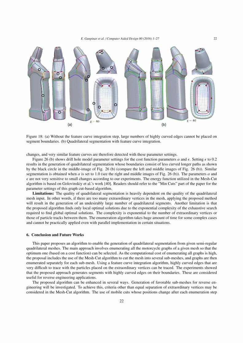
As detailed in the feature curve integration algorithm, it is crucial to place particles on highly curved regions thatcannot be traced by particles placed on extraordinary vertices. Figure 18 (a) shows such a case for the bottle model.

16


Figure 14: Feature curves (in blue) in the mesh that are not close to extraordinary vertices are extracted. Two particlesmoving in opposite directions (a) are placed next to the middle of the curve.

A large number of highly curved edges (marked with black circles) can be seen inside the generated segments, whichis problematic for B-spline surface fitting. The feature curve integration step improves the quality of quadrilateralsegmentation (b) for reverse engineering applications.

Different quadrilateral segmentations are obtained when χ is set to 20, 40 and 60 as shown in Figure 19 (a), (b)and (c). However, highly curved edges in the model are captured for all these χ settings. The quadrilateral segmentsgenerated using the motorcycle graph algorithm [3] (d), method of [22] ((e), for their particular choice of thresholds),method of Campen et al. [26] ((f), for their particular choice of thresholds) and method of Bommes et al. [19] ((g), fortheir particular choice of thresholds) have highly curved edges seen in the inner regions (marked with black circles)which may not be generally preferable for surface fitting in practice. Quadrilateral segments generated using othermethods ( [23, 25]) also contain these highly curved edges as far as their images shown in the papers are concerned.Recall that T-junctions do not exist in the partitions of [25, 23, 26], whereas they exist in that of [22, 3] and theproposed method.

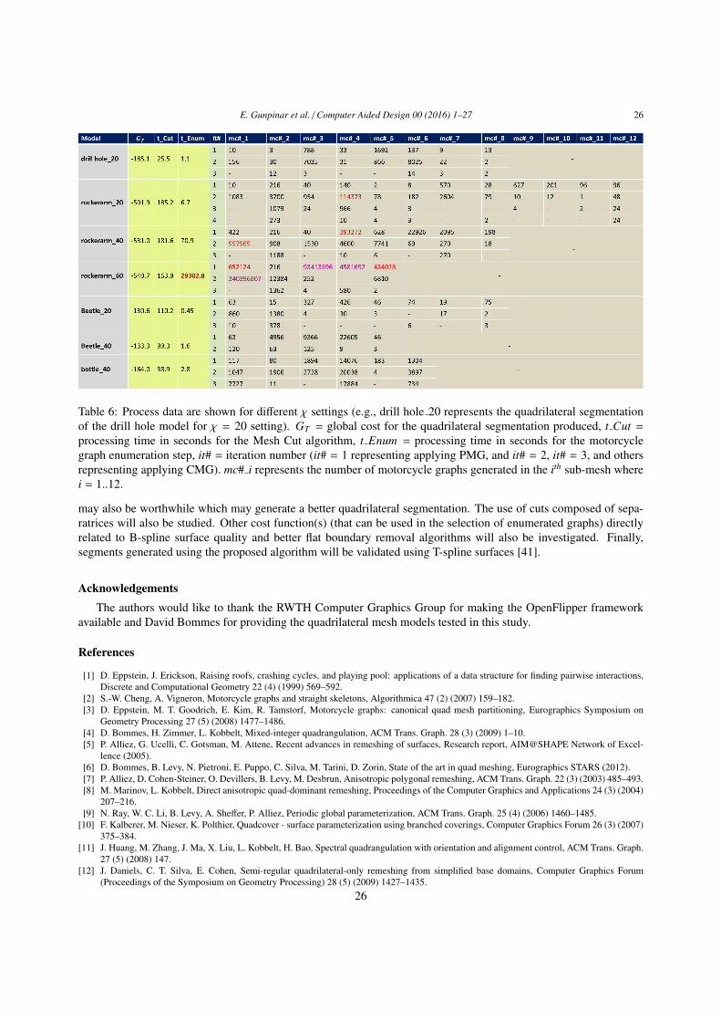
Computational time: A PC having Intel Core i5 650 3.2 GHz processor and 16 GB memory is used for theexperiments in this study and the implementation is single-threaded. Table 6 shows the computational time taken foreach model. The processing time for the Mesh Cut algorithm depends on the χ setting, and is much longer for smallervalues because the mesh is cut into a large number of sub-meshes. Computation of the geodesic distance from eachvertex in the mesh to the source and sink terminals dominates the processing time in this step. The motorcycle graphenumeration step also depends on the χ settings, and the computational cost is higher for greater values because alarge number of graphs are enumerated. As an example, for rockerarm model with χ = 60, 340, 396, 807 motorcyclegraphs were enumerated at a time cost of more than eight hours. However, the test results indicate that, better solutions(with minimum cost) were obtained with large χ values (compare the costs of rockerarm with χ = 20, 40, 60 and theBeetle with χ = 20, 40). For the drill hole and bottle models, the results are very similar when χ is set to 20, 40 or 60.Assigning large values such as 80 for χ results in such high computational cost that the graph enumeration step takesa large amount of time.

Flat boundary removal: To achieve a quadrilateral segmentation with much greater compactness (i.e., fewersegments), flat (less-curved) boundaries are removed using a naive approach. Any particle tracks with a cost exceedingthe user-defined parameter η are removed (η = 1 for the drill hole and bottle models, and η = −3 for the rockerarm andBeetle models). A greedy removal process is applied in which tracks are sorted in decreasing order of cost and thosewith higher cost are removed first. If non-quadrilateral segments occur during this process, removal is not performed.The images on the top of Fig. 20 (a) show the models after this process.

By removing a path, the shape of the boundary may become worse in termsof the reverse engineering. An additional criterion called as boundary smoothnesscriterion is considered during the removal process. If a sharp corner (like a kink)occurs on the boundary after this process, the removal is discarded. We simplycheck the angle between two neighboring edges (in red and orange on the rightimage) of the first and last edge (in black) in the paths. If this angle is larger thanthe parameter P (set to 25 degree), removal is discarded. Otherwise, it is performed. Bottom images of Figure 20 (a)

17


Figure 15: (a) The initial mesh with its base complex is given. The total number of ordinary junctions is 1344. (b)Feature curves far away from extraordinary vertices are detected. Particles moving in opposite directions are placedon the middle of these feature curves in opposite directions and on extraordinary vertices. (c) To obtain sub-mesheswith simpler base complexes, the mesh is cut into several sub-meshes each with the desired base complex complexity.A total of 8 sub-meshes are obtained with 45 ordinary junctions. (d) The base complex for each sub-mesh is found. (e)Optimum motorcycle graphs are enumerated for each sub-mesh. After several enumerations, a motorcycle graph ofthe initial mesh is obtained. (f) Flat particle tracks are removed and a much more compact quadrilateral segmentationis achieved. (g) Generated partitions are validated with B-spline surfaces.

Figure 16: Motorcycle graph enumeration steps for a Beetle model (χ = 60). Enumerations are performed in eachsub-mesh separately using the relevant computed base complexes (images on the left in (a-1), (a-2), (a-3) and (a-4)),and graphs are generated in each sub-mesh (images on the right in (a-1), (a-2), (a-3) and (a-4)). To obtain a motorcyclegraph of a given mesh, enumerations are performed once more ((b-1), (b-2), (b-3) and (b-4)).

shows partitions when the boundary smoothness criterion is used. As a part of the future work, we will investigatealgorithms considering several criteria during removal process. The parameters η and P are not sensitive to smallchanges.

B-spline surfaces: Without the parameterization step, B-spline surfaces can be generated as they intrinsicallyhave parameter u − v values. Each segment is fitted with uniform bi-cubic B-spline surfaces, and segments have datapoints regularly located in the u−v direction. Two-stage curve blending is performed such that data in each u directionare blended to form a curve, and these curves are then blended to form a surface.

Let a quadrilateral segment have (m + 1) × (n + 1) data points Pi, j where 0 ≤ i ≤ m and 0 ≤ j ≤ n representingindices of columns and rows respectively. The following linear system is first solved under the free-end condition to

18


Figure 17: Setting small values for χ creates narrow search spaces for sub-meshes. For χ = 20 (b), the cut markedwith the red circle does not allow the particle (track marked with a black circle) to go further and trace the highlycurved edges (marked with black round dots) traced when χ = 20 (a). The proposed algorithm (a) generates a betterquadrilateral segmentation than the motorcycle graph algorithm [3] (c). Highly curved edges are present inside thesegments marked with a black circle.

obtain control points < C0, j,C1, j,C2, j, . . . ,Cm+1, j,Cm+2, j >:

1 −1 0 0 · · · 01 4 1 0 · · · 00 1 4 1 · · · 0...

......

.... . .

...0 · · · 0 1 4 10 · · · 0 0 −1 1

×

C0, jC1, jC2, j...

Cm+1, jCm+2, j

=

06P0, j6P1, j...

6Pm+1, j0

.

The obtained control points Ci, j are again blended for all columns by solving the following linear system under thefree-end condition to obtain final control points < Vi,0,Vi,1,Vi,2, . . . ,Vi,n+1,Vi,n+2 > of uniform cubic B-spline surface:

1 −1 0 0 · · · 01 4 1 0 · · · 00 1 4 1 · · · 0...

......

.... . .

...0 · · · 0 1 4 10 · · · 0 0 −1 1

×

Vi,0Vi,1Vi,2...

Vi,n+1Vi,n+2

=

06Ci,06Ci,1...

6Ci,n

0

.

Figure 20 (b) and Figure 15 (g) show B-spline surfaces for segments generated using the proposed algorithm.Deviation of the generated surfaces from the original quadrilateral mesh is shown in Fig. 21. Less deviation occurswith segments generated using the proposed algorithm (PA) than with those generated using the bi-monotone segmentgeneration method [38] (for the particular choice of thresholds used in the paper) and the motorcycle graph (MC)algorithm [3].

Comparison with existing techniques: Approaches with functions similar to that of the proposed method havebeen reported by Myles et al. [22] and Gunpinar et al. [39]. In the former, highly curved regions are implicitlyplaced on quadrilateral segment boundaries. Due to the methodologies used in the approach, highly-curved regionsare sometimes seen within the boundaries of these segments (see Figure 19 (e)). As the geometric error (i.e., εP)is measured as an area-weighted error during T-mesh optimization, the geometric constraint parameter (i.e., ε0) alsoworks as an area-weighted quantity. It is considered difficult to control ordinary (non-area-weighted) geometric errorby specifying an area-weighted error, which in turn makes the placement of highly-curved regions on boundariesdifficult. Precise surface approximation error is also not utilized because of its computational complexity. Instead, asimple Bezier curve network fit is used to approximate the per-patch error, which additionally makes it more difficultto control the exact geometric error. As shown by the images in [22], an undesirably large number of quadrilateralsegments is needed to capture all highly curved regions in the model. This stems from the energy formula utilized,which favors square quadrilateral segments based on the perimeter-area ratio. In contrast, quadrilateral segment shapesare determined from feature curves in the proposed algorithm, and elongated features (such as fillets) can thereforebe captured by a single quadrilateral segment. The proposed method is based on motorcycle graphs, which have the

19


potential advantage of theoretically guaranteed coarseness shown by Eppstein et al. (i.e. the number of patches inmotorcycle graphs is within a constant factor of the optimum).

The proposed method and the technique of Gunpinar et al. [39] can be compared in terms of the cost value ofthe quadrilateral segmentation generated. The parameters in the headers of Table 3 (GTPF , GT20 and GT40 ) refer tothe global cost for the quadrilateral segments obtained using [39], and for that of the proposed method with χ = 20and χ = 40, respectively. All values are obtained without using the feature curve integration algorithm becauseboth techniques involve slightly different methodologies to for feature curve detection. The proposed algorithm withχ = 40 allows a lower quadrilateral segmentation cost than Gunpinar et al.’s technique [39] thanks to its enumerationalgorithm, which looks for an optimum motorcycle graph over a wider solution space rather than utilizing a greedylocal path flipping operator. For the χ = 20 setting, the quadrilateral segmentation generated for some test modelshas a higher cost than those obtained with Gunpinar et al.’s technique [39] as this χ setting leads to the formation oflarge numbers of sub-meshes with narrower search spaces. Figure 22 shows quadrilateral segments generated usingboth techniques. The proposed algorithm exhibits better performance in terms of capturing and placing highly-curvedparts on quadrilateral segment boundaries as shown by the black circles.

Models GTPF GT20 GT40

drill hole -168.156 -177.701 -177.701rockerarm -382.521 -374.43 -397.581Beetle -25.8289 -18.9696 -46.038bottle 131.407 138.529 131.201

Table 3: Global cost values (GTPF , GT20 and GT40 ) after applying the Gunpinar et al.’s technique [39] and the proposedmethod with χ = 20 and χ = 40, respectively.

Comparison of results with optimum solutions: The results of quadrilateral segmentation using the proposedenumeration algorithm as described in Section 4 with the Mesh-Cut algorithm are here compared with those obtainedwithout the Mesh-Cut algorithm (full enumeration). A block model generated using [19], a partial Beetle modelobtained using [4] and a partial drill hole model generated using [23] are tested using a PC with an Intel Core i5 32302.6 GHz processor and 8 GB of memory. As seen from Figure 23, the results of both approaches are similar. Table4 lists the costs of the quadrilateral segmentations obtained and the related processing times. It can be seen that theenumeration algorithm with the Mesh-Cut algorithm is very efficient in terms of the time required for computation,and the solutions obtained converge or are very close to global optimum when χ has larger values. By way of example,full enumeration takes almost five days for the partial drill hole model, and a global optimum solution is obtained. Thesame solution is reached when the proposed enumeration algorithm is used with the Mesh-Cut algorithm (χ = 60),and the computational time is about five seconds. The proposed algorithm is used without the feature curve integrationalgorithm for the block model, and highly-curved regions (shown by black dots) are not captured with the motorcycleedges (edges shown by yellow dashes are less curved). The processing time for full enumeration of the block modelis less than two hours. This is because its base complex is much coarser than the other models in this paper, with themean and maximum lengths of separatrices being 1.46 and 3, respectively. Note that it may not always be possibleto obtain a quadrilateral segmentation that converges or is very close to the global optimum when the Mesh-Cutalgorithm is used.

Evaluation of various cuts: The enumeration algorithm described in Section 4.2.2 is used with two Mesh-Cutalgorithms different from the one outlined in Section 4.2.1, and the quadrilateral segmentations generated are analyzed.The two proposed Mesh-Cut algorithms set source and sink terminals differently so that cuts differing from thoseproduced using the algorithm described in Section 4.2.1 are generated. After terminals are assigned, the same energyfunction is utilized for these two algorithms. In the first algorithm, the source and sink terminals are selected as thefarthest vertices in a mesh or sub-mesh that will be cut into two in the next step. The convex hull of the mesh orsub-mesh is used in order to reduce computational complexity for farthest pair computation, and terminal vertices arefound. Figure 24 (a) shows a cut and terminal vertices generated using this method for a drill hole model. In the secondalgorithm, three different cuts (see CutX, CutY and CutZ in Figure 24 (b), (c) and (d), respectively) are generated usingthe bounding box (BB) of the model. For example, the source and sink terminals used for the computation of CutX

20


Models GT tp

block (χ = 20) 105.16 7 minsblock (χ = 100) 102.013 2 mins 30 secsblock (χ = 120) 102.013 2 mins 7 secsblock (Full) 101.636 1 hour 44 mins 53 secsBeetlepartial (χ = 20) 1.53841 15 secsBeetlepartial (Full) 1.53841 8 hours 17 mins 36 secsdrill holepartial (χ = 20) -73.8992 4.7 secsdrill holepartial (χ = 60) -92.3255 5.1 secsdrill holepartial (Full) -92.3255 4 days 23 hours 25 mins 18 secs

Table 4: Cost values (GT ) of the quadrilateral segmentations obtained and the processing times (tp) for the enumerationalgorithm with (χ) and without(Full) the Mesh-Cut algorithm. Beetlepartial and drill holepartial denote that partialmodels are used for the Beetle and drill hole models.

are the vertices closest to Xmax and Xmin, which are the center vertices on the BB walls as shown in Fig. 24 (b). Theterminals used for the computation of CutY and CutZ are selected in a similar way. One of these three cuts is selectedas the final cut that generates sub-meshes with less complicated base complexities (see quasi-complexity U in Section4.2.1). Two sub-meshes are generated after a cut operation, and the one with a more complicated base complex ischosen for comparison of the base complexes obtained after the application of these three cuts.

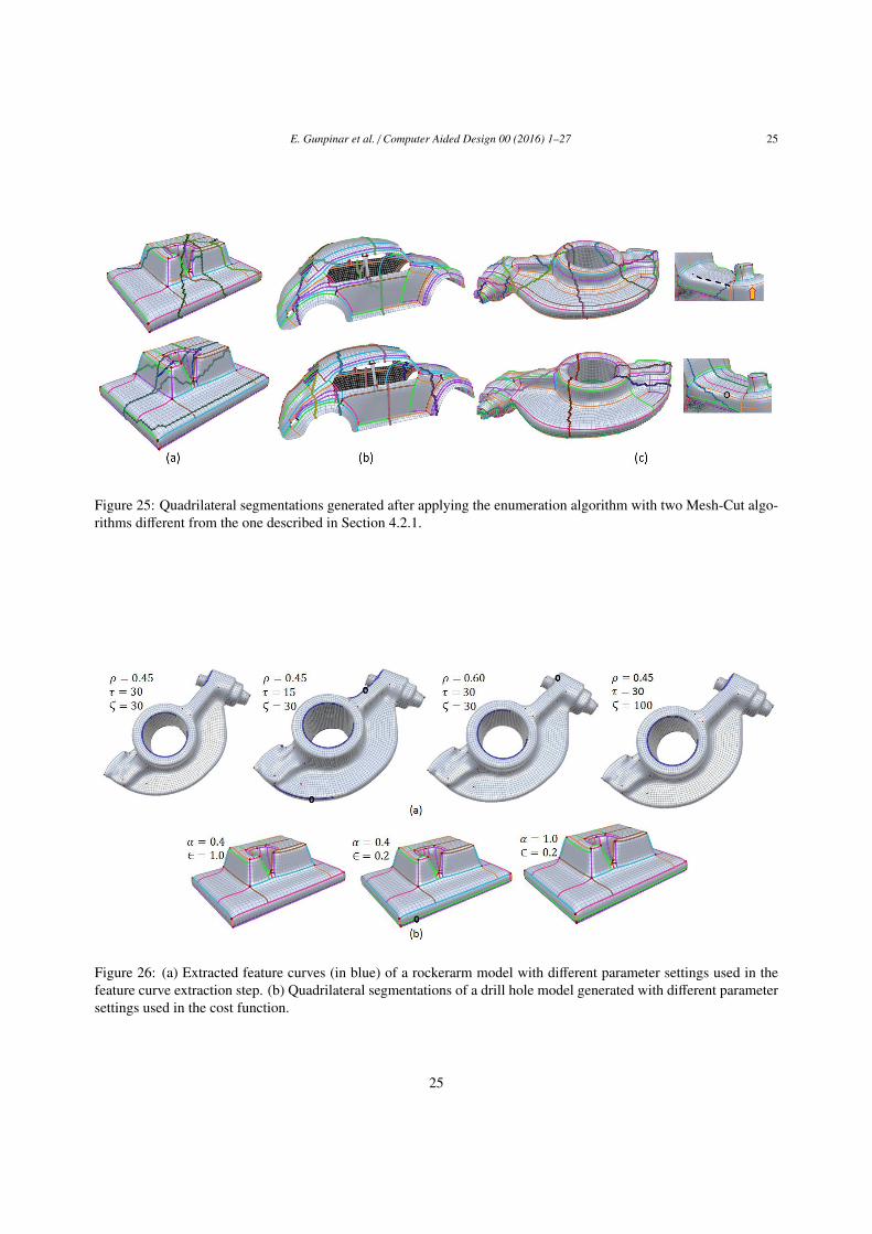
Figure 25 shows the quadrilateral segmentations obtained after applying the enumeration algorithm to the sub-meshes generated using these Mesh-Cut algorithms. Table 5 shows the cost values (GT20 , GTo1 , GTo2 , respectively)observed when the enumeration algorithm is used with the Mesh-Cut algorithm as described in Section 4.2.1 andwhen two different Mesh-Cut methods are utilized (with a setting of χ = 20). Although generally similar cost valuesare obtained, a smaller value is achieved for GTo2 in the rockerarm model. The position of the cuts obtained affectsthe quadrilateral segmentation generated. In the top-right image of Fig. 25 (c), the particle track shown in orange(indicated with an arrow) cannot grow because of the cut in blue, and highly-curved edges shown with dashed linesare not traced. The same track grows through these highly curved edges if the cut does not cross them (see thebottom-right image in Fig. 25 (c)). However, it is not always possible to obtain such cuts due to the presence oflarge numbers of feature curves in the model. According to our experiments, the most significant way of generatinga higher-quality quadrilateral segmentation is to set larger values for χ in the Mesh-Cut step, which leads to thegeneration of sub-meshes with wider search spaces (see Figures 17 and 19).

Models GT20 GTo1 GTo2

drill hole -185.1 -184.179 -182.362Beetle -130.6 -128.449 -128.348rockerarm -501.9 -502.181 -525.389

Table 5: The cost values (GT20 , GTo1 , GTo2 , respectively) adopted when the enumeration algorithm is used with theMesh-Cut algorithm described in Section 4.2.1 and two different Mesh-Cut methods are utilized.

Parameter tuning: Several parameter tuning experiments are carried out to verify the parameters presented in thispaper. Figure 26 (a) shows a rockerarm model with extracted feature curves indicated in blue for different parametersettings. Setting higher flatness values enables extraction limited to more highly-curved feature curves. The featurecurve shown by the black circle in the middle right image of Fig. 26 (c) cannot be traced when ρ is set to 0.6, but istraced when ρ = 0.45 (see the left- and middle-right images of Fig. 26 (a)). Setting the threshold τ to smaller valuesenables extraction of shorter feature curves. The middle-left image of Fig. 26 (a) shows feature curves (depicted byblack circles) captured when τ is set to 15 but not captured when τ = 30 (see the left- and middle- left images of Fig.26 (a)). Similar feature curves are obtained when setting the parameter ζ to 30 and 100 (see the images on the leftand right of Fig. 26 (a)). According to our experience, parameter tuning for ρ, τ and ζ is not very sensitive to small

21


Figure 18: (a) Without the feature curve integration step, large numbers of highly curved edges cannot be placed onsegment boundaries. (b) Quadrilateral segmentation with feature curve integration.

changes, and very similar feature curves are therefore detected with these parameter settings.Figure 26 (b) shows drill hole model parameter settings for the cost function parameters α and ε. Setting ε to 0.2

results in the generation of quadrilateral segmentation whose boundaries consist of less curved longer paths as shownby the black circle in the middle-image of Fig. 26 (b) (compare the left and middle images of Fig. 26 (b)). Similarsegmentation is obtained when α is set to 1.0 (see the right and middle images of Fig. 26 (b)). The parameters α andε are not very sensitive to small changes according to our experiments. The energy function utilized in the Mesh-Cutalgorithm is based on Golovinskiy et al.’s work [40]. Readers should refer to the ”Min Cuts” part of the paper for theparameter settings of this graph cut-based algorithm.

Limitations: The quality of quadrilateral segmentation is heavily dependent on the quality of the quadrilateralmesh input. In other words, if there are too many extraordinary vertices in the mesh, applying the proposed methodwill result in the generation of an undesirably large number of quadrilateral segments. Another limitation is thatthe proposed algorithm finds only local optimal solutions due to the exponential complexity of the exhaustive searchrequired to find global optimal solutions. The complexity is exponential to the number of extraordinary vertices orthose of particle tracks between them. The enumeration algorithm takes huge amount of time for some complex casesand cannot be practically applied even with parallel implementation in certain situations.

6. Conclusion and Future Works

This paper proposes an algorithm to enable the generation of quadrilateral segmentation from given semi-regularquadrilateral meshes. The main approach involves enumerating all the motorcycle graphs of a given mesh so that theoptimum one (based on a cost function) can be selected. As the computational cost of enumerating all graphs is high,the proposal includes the use of the Mesh-Cut algorithm to cut the mesh into several sub-meshes, and graphs are thenenumerated separately for each sub-mesh. Using a feature curve integration algorithm, highly curved edges that arevery difficult to trace with the particles placed on the extraordinary vertices can be traced. The experiments showedthat the proposed approach generates segments with highly curved edges on their boundaries. These are considereduseful for reverse engineering applications.

The proposed algorithm can be enhanced in several ways. Generation of favorable sub-meshes for reverse en-gineering will be investigated. To achieve this, criteria other than equal separation of extraordinary vertices may beconsidered in the Mesh-Cut algorithm. The use of mobile cuts whose positions change after each enumeration step

22


Figure 19: Diverse quadrilateral segmentations (a, b, c) are obtained for different χ settings (20, 40, 60). Segmentsgenerated using the motorcycle graph algorithm [3] (d), the method of [22] (e), the method of [26] (f) and the methodof [19] (g) contain highly curved edges in the inner regions (marked with black circles) which may not be generallypreferable for surface fitting in practice.

Figure 20: (a) Partitions after removal of flat (less curved) paths without consideration of the boundary smoothnesscriterion (top) and with consideration (bottom). (b) B-spline surfaces (in blue) fitted to these segments.

Figure 21: Less deviation is observed for segments generated using the proposed algorithm (PA) than for thosegenerated using the bi-monotone segment generation method [38] and the motorcycle graph (MC) algorithm (seelocations marked with black circles).

23


Figure 22: Comparison between the proposed algorithm and the method of Gunpinar et al. [39]: The proposedalgorithm in this paper has better performance in terms of capturing and placing highly-curved parts on the segmentboundaries. The parts shown with black circle are captured using the proposed algorithm (right figures in (a, b)),whereas the technique [39] does not capture these highly-curved regions (left figures in (a, b)).

Figure 23: The identical or similar quadrilateral segmentations are obtained when the enumeration algorithm is usedwith(χ) and without(Full) the Mesh-Cut algorithm.

Figure 24: (a) A cut generated by selecting source and sink terminals as the farthest vertices in the mesh. (b) Thesource and sink terminals used for the computation of CutX are the vertices closest to Xmax and Xmin, which are thecenter vertices on the walls of the model bounding box. (c, d) The terminals used for the computation of CutY andCutZ are selected in a similar way.

24


Figure 25: Quadrilateral segmentations generated after applying the enumeration algorithm with two Mesh-Cut algo-rithms different from the one described in Section 4.2.1.

Figure 26: (a) Extracted feature curves (in blue) of a rockerarm model with different parameter settings used in thefeature curve extraction step. (b) Quadrilateral segmentations of a drill hole model generated with different parametersettings used in the cost function.

25


Table 6: Process data are shown for different χ settings (e.g., drill hole 20 represents the quadrilateral segmentationof the drill hole model for χ = 20 setting). GT = global cost for the quadrilateral segmentation produced, t Cut =

processing time in seconds for the Mesh Cut algorithm, t Enum = processing time in seconds for the motorcyclegraph enumeration step, it# = iteration number (it# = 1 representing applying PMG, and it# = 2, it# = 3, and othersrepresenting applying CMG). mc# i represents the number of motorcycle graphs generated in the ith sub-mesh wherei = 1..12.

may also be worthwhile which may generate a better quadrilateral segmentation. The use of cuts composed of sepa-ratrices will also be studied. Other cost function(s) (that can be used in the selection of enumerated graphs) directlyrelated to B-spline surface quality and better flat boundary removal algorithms will also be investigated. Finally,segments generated using the proposed algorithm will be validated using T-spline surfaces [41].

AcknowledgementsThe authors would like to thank the RWTH Computer Graphics Group for making the OpenFlipper framework

available and David Bommes for providing the quadrilateral mesh models tested in this study.

References

[1] D. Eppstein, J. Erickson, Raising roofs, crashing cycles, and playing pool: applications of a data structure for finding pairwise interactions,Discrete and Computational Geometry 22 (4) (1999) 569–592.

[2] S.-W. Cheng, A. Vigneron, Motorcycle graphs and straight skeletons, Algorithmica 47 (2) (2007) 159–182.[3] D. Eppstein, M. T. Goodrich, E. Kim, R. Tamstorf, Motorcycle graphs: canonical quad mesh partitioning, Eurographics Symposium on

Geometry Processing 27 (5) (2008) 1477–1486.[4] D. Bommes, H. Zimmer, L. Kobbelt, Mixed-integer quadrangulation, ACM Trans. Graph. 28 (3) (2009) 1–10.[5] P. Alliez, G. Ucelli, C. Gotsman, M. Attene, Recent advances in remeshing of surfaces, Research report, AIM@SHAPE Network of Excel-

lence (2005).[6] D. Bommes, B. Levy, N. Pietroni, E. Puppo, C. Silva, M. Tarini, D. Zorin, State of the art in quad meshing, Eurographics STARS (2012).[7] P. Alliez, D. Cohen-Steiner, O. Devillers, B. Levy, M. Desbrun, Anisotropic polygonal remeshing, ACM Trans. Graph. 22 (3) (2003) 485–493.[8] M. Marinov, L. Kobbelt, Direct anisotropic quad-dominant remeshing, Proceedings of the Computer Graphics and Applications 24 (3) (2004)

207–216.[9] N. Ray, W. C. Li, B. Levy, A. Sheffer, P. Alliez, Periodic global parameterization, ACM Trans. Graph. 25 (4) (2006) 1460–1485.

[10] F. Kalberer, M. Nieser, K. Polthier, Quadcover - surface parameterization using branched coverings, Computer Graphics Forum 26 (3) (2007)375–384.

[11] J. Huang, M. Zhang, J. Ma, X. Liu, L. Kobbelt, H. Bao, Spectral quadrangulation with orientation and alignment control, ACM Trans. Graph.27 (5) (2008) 147.

[12] J. Daniels, C. T. Silva, E. Cohen, Semi-regular quadrilateral-only remeshing from simplified base domains, Computer Graphics Forum(Proceedings of the Symposium on Geometry Processing) 28 (5) (2009) 1427–1435.

26


[13] M. Zhang, J. Huang, X. Liu, H. Bao, A wave-based anisotropic quadrangulation method, ACM Trans. Graph. 29 (4) (2010) 1–8.[14] D. Kovacs, A. Myles, D. Zorin, Anisotropic quadrangulation, Computer Aided Geometric Design 28 (8) (2011) 449–462.[15] A. Myles, D. Zorin, Global parameterization by incremental flattening, ACM Trans. Graph. 31 (4) (2012) 1–11.[16] N. Kowalski, F. Ledoux, P. Frey, A pde based approach to multidomain partitioning and quadrilateral meshing, Proceedings of the 21st

International Meshing Roundtable (2013) 137–154.[17] D. Panozzo, Y. Lipman, E. Puppo, D. Zorin, Fields on symmetric surfaces, ACM Trans. Graph. 31 (4).[18] M. Zhang, J. Huang, X. Liu, H. Bao, A divide-and-conquer approach to quad remeshing, IEEE Transactions on Visualization and Computer

Graphics 99.[19] D. Bommes, M. Campen, H. Ebke, P. Alliez, L. Kobbelt, Integer-grid maps for reliable quad meshing, ACM Transactions on Graphics 32 (4)

(2013) 98.[20] J. Daniels, C. T. Silva, J. Shepherd, E. Cohen, Quadrilateral mesh simplification, ACM Trans. Graph. 27 (5).[21] M. Tarini, N. Pietroni, P. Cignoni, D. Panozzo, E. Puppo, Practical quad mesh simplification, Computer Graphics Forum 29 (2) (2010)

407–418.[22] A. Myles, N. Pietroni, D. Kovacs, D. Zorin, Feature-aligned t-meshes, ACM Trans. Graph. 29 (4) (2010) 1–11.[23] D. Bommes, T. Lempfer, L. Kobbelt, Global structure optimization of quadrilateral meshes, Computer Graphics Forum 30 (2) (2011) 375–

384.[24] C. Peng, E. Zhang, Y. Kobayashi, P. Wonka, Connectivity editing for quadrilateral meshes, ACM Trans. Graph. 30 (6) (2011) 141.[25] M. Tarini, E. Puppo, D. Panozzo, N. Pietroni, P. Cignoni, Simple quad domains for field aligned mesh parametrization, ACM Trans. Graph.

30 (6) (2011) 142.[26] M. Campen, D. Bommes, L. Kobbelt, Dual loops meshing: quality quad layouts on manifolds, ACM Trans. Graph. 31 (4) (2012) 1–11.[27] A. Agathos, I. Pratikakis, S. Perantonis, N. Sapidis, P. Azariadis, 3d mesh segmentation methodologies for CAD applications, Computer

Aided Design And Applications 4 (6) (2007) 827–841.[28] A. Shamir, A survey on mesh segmentation techniques, Computer Graphics Forum 27 (6) (2008) 1539–1556.[29] A. Mangan, R. T. Whitaker, Partitioning 3d surface meshes using watershed segmentation, IEEE Transactions on Visualization and Computer

Graphics 5 (4) (1999) 308–321.[30] M. Garland, A. Willmott, P. S. Heckbert, Hierarchical face clustering on polygonal surfaces, Symposium on Interactive 3D Graphics (2001)

49–58.[31] Y. Boykov, V. Kolmogorov, An experimental comparison of min-cut/max-flow algorithms for energy minimization in vision, IEEE Transac-

tions on Pattern Analysis and Machine Intelligence 26 (9) (2004) 1124–1137.[32] D. Cohen-Steiner, P. Alliez, M. Desbrun, Variational shape approximation, ACM Transactions on Graphics 23 (3) (2004) 905–914.[33] P. Benko, T. Varady, Direct segmentation of smooth, multiple point regions, Geometric Modeling and Processing (2002) 169–178.[34] J. H. Wu, L. Kobbelt, Structure recovery via hybrid variational surface approximation, Computer Graphics Forum 24 (3) (2005) 277–284.[35] S. Katz, A. Tal, Hierarchical mesh decomposition using fuzzy clustering and cuts, ACM Transactions on Graphics (TOG) 22 (3) (2003)

954–961.[36] H. Hoppe, T. DeRose, T. Duchamp, M. Halstead, H. Jin, J. McDonald, J. Schweitzer, W. Stuetzle, Piecewise smooth surface reconstruction,

Proceedings of the 21st annual conference on Computer graphics and interactive techniques (1994) 295–302.[37] H. Pottmann, S. Leopoldseder, M. Hofer, Approximation with active b-spline curves and surfaces, Proceedings of the 10th Pacific Conference

on Computer Graphics and Applications (2002) 8–25.[38] E. Gunpinar, H. Suzuki, Y. Ohtake, M. Moriguchi, Generation of bi-monotone patches from quadrilateral mesh for reverse engineering,

Computer-Aided Design 45 (2) (2013) 440–450.[39] E. Gunpinar, M. Moriguchi, H. Suzuki, Y. Ohtake, Feature-aware partitions from motorcycle graph, Computer-Aided Design 47 (2014)

85–95.[40] A. Golovinskiy, T. Funkhouser, Randomized cuts for 3d mesh analysis, ACM Transactions on Graphics (2008) 27 (5).[41] T. Sederberg, J. Zheng, A. Bakenov, A. Nasri, T-splines and T-NURCCs, ACM Trans. Graph. 22 (3) (2003) 477–484.

27

Date post:	12-Mar-2018
Category:	Documents
Upload:	vuongtruc
View:	214 times
Download:	0 times

Motorcycle Graph Enumeration from Quadrilateral …scad.itu.edu.tr/1/images/PDF3.pdfComputer Aided...

Documents