1. Overview of multiple regression and multiple correlation
2. Applications and Implications
3. General Linear Model Approach Using MRC Analysis
4. Example From Kirk (and Topic 3)Effect CodingDummy Coding
5. Assumptions
2
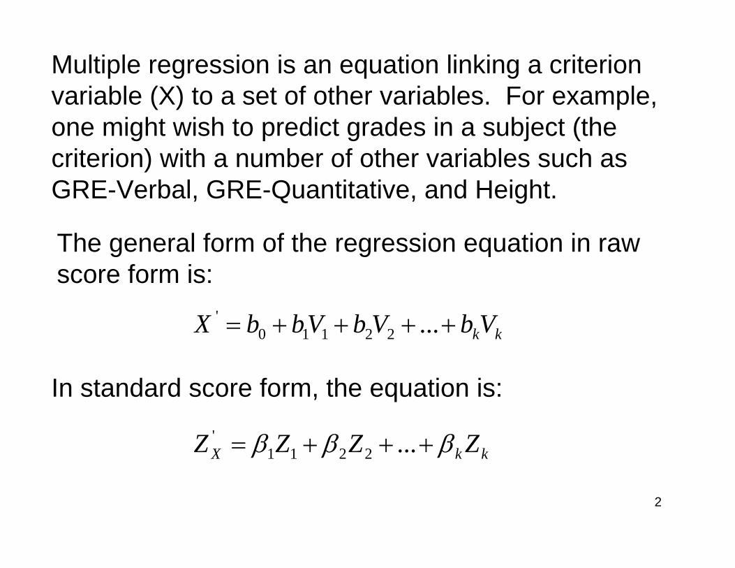
Multiple regression is an equation linking a criterion variable (X) to a set of other variables. For example, one might wish to predict grades in a subject (the criterion) with a number of other variables such as GRE-Verbal, GRE-Quantitative, and Height.
The general form of the regression equation in raw score form is:
kkVbVbVbbX ++++= ...22110'
In standard score form, the equation is:
kkX ZZZZ βββ +++= ...2211'
3
Multiple Correlation is the Pearson product moment correlation of the obtained and predicted values of X.
'
'' ))((
XX SnSXXXX
R ∑ −−=
The test of significance of the multiple correlation is:
)1/(²)1(/²
−−−=
pNRpRF
where : R² = R² X.V1,V2,…
p = number of predictor variables
N = the total number of observations
4
With a bit of algebra, R can be shown to equal:
kXkXX rrrR βββ +++= ...2211
And that:X
kkk S
Sb=β
That is, the multiple correlation is equal to the square root of the sum of the product of the standardized regression coefficient for each predictor times its correlation with the criterion.
That is, the standardized regression coefficient for a predictor is equal to its unstandardized regression coefficient times its standard deviation divided by the standard deviation of the criterion.
5
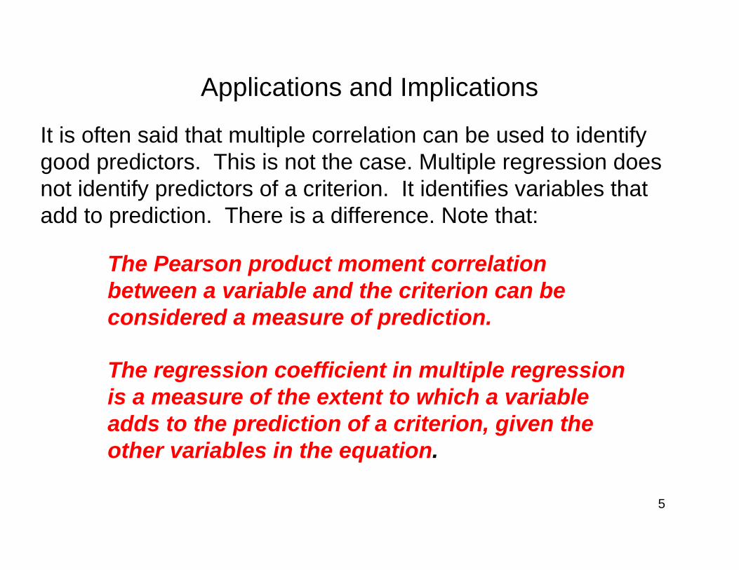
Applications and Implications
It is often said that multiple correlation can be used to identify good predictors. This is not the case. Multiple regression doesnot identify predictors of a criterion. It identifies variables that add to prediction. There is a difference. Note that:
The Pearson product moment correlation between a variable and the criterion can be considered a measure of prediction.
The regression coefficient in multiple regression is a measure of the extent to which a variable adds to the prediction of a criterion, given the other variables in the equation.
6
General Linear Model Approach
The Model: Analysis of variance can be seen as an instance of the general linear model.
Thus, Cohen & Cohen (1983, p. 4) state “Technically, AV/ACV and conventional multiple regression analysis are special cases of the “general linear model” in mathematical statistics. It thus follows that any data analyzable by AV/ACV may be analyzed by MRC, while the reverse is not the case”.
In a more recent edition of the book, Cohen, Cohen, West & Aiken (2003, p. 4) state” The description of MRC in this book includes extensions of conventional MRC analysis to the point where it is essentially equivalent to the general linear model. It thus follows that any data analyzable by ANOVA/ANCOVA may be analyzed by MRC, whereas the reverse is not the case”.
7
MRC Analysis
Cohen (1968) noted that, if group membership is defined in terms of a series of arbitrary variables (A), analysis of variance can be viewed as a special case of multiple regression. Thus, one can write a regression equation as:
ioi AbAbbX ε++++= ...2211
where the number of arbitrary variables is one less than the number of treatment levels. The predicted value for each individual is the mean of the treatment condition for that individual and the A variables are codes defining the treatment levels.
8
0010
0100
1000
1234
A3A2A1Treatment
Dummy Coding
001-1
010-1
100-1
1234
A3A2A1Treatment
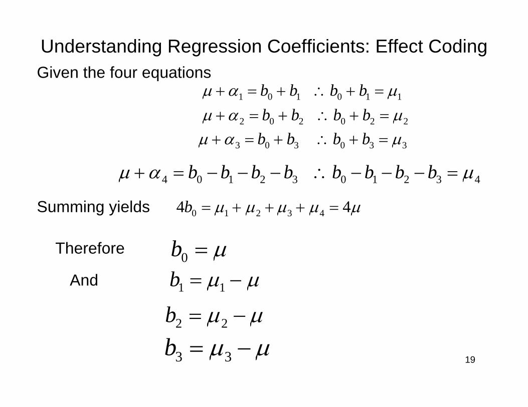
Effect Coding
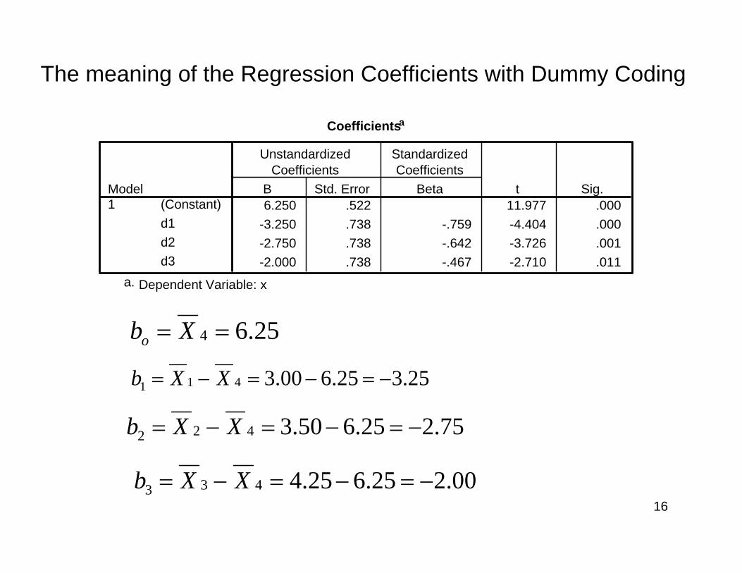
Types of Coding: There are many types of coding. Each yield the same multiple correlation but the regression coefficients differ. We will consider two types, Dummy Coding and Effect Coding.Following are two examples involving 4 treatment levels of a factor.
9
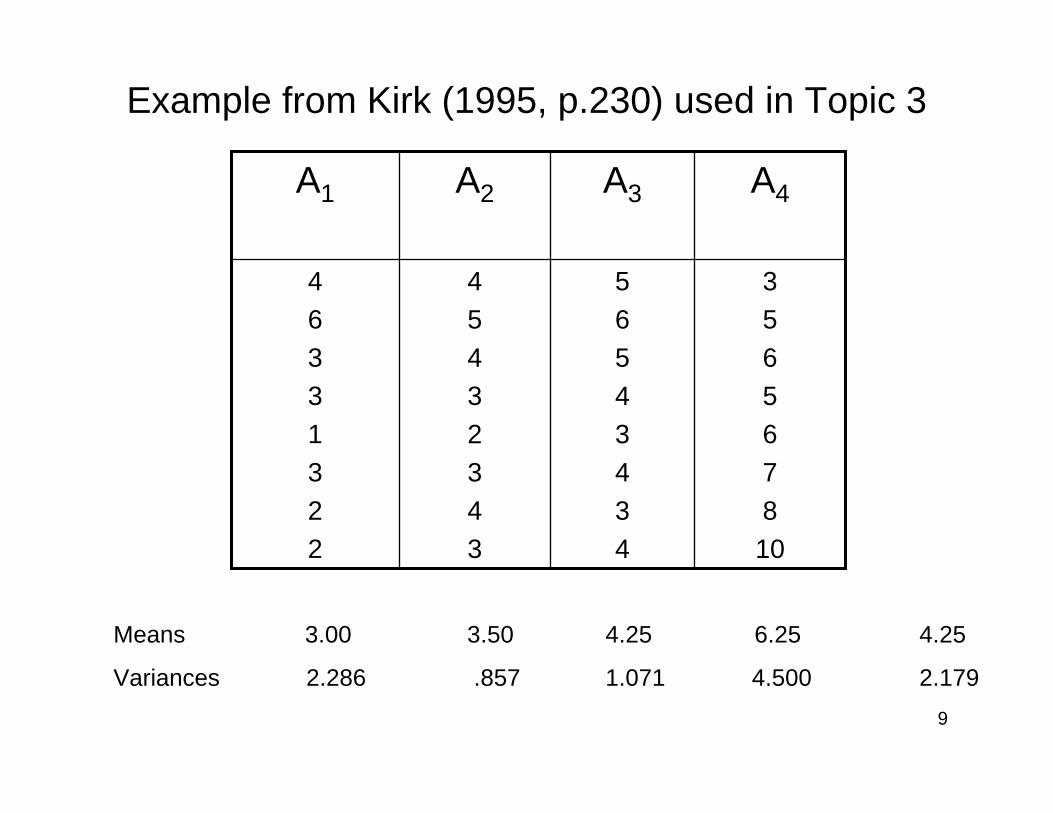
356567810
56543434
45432343
46331322
A4A3A2A1
Means 3.00 3.50 4.25 6.25 4.25
Variances 2.286 .857 1.071 4.500 2.179
Example from Kirk (1995, p.230) used in Topic 3
10
Data Editor with first 4 Subjects for each treatment showing both Dummy and Effect coding
11
GETFILE='F:\PSYCH540\kirkdata171.sav'.
DATASET NAME DataSet1 WINDOW=FRONT.REGRESSION/DESCRIPTIVES MEAN STDDEV CORR SIG N/MISSING LISTWISE/STATISTICS COEFF OUTS R ANOVA/CRITERIA=PIN(.05) POUT(.10)/NOORIGIN/DEPENDENT x/METHOD=ENTER e1 e2 e3 .
SourceCorrected ModelInterceptbErrorTotalCorrected Total
Type III Sumof Squares df Mean Square F Sig.
R Squared = .445 (Adjusted R Squared = .386)a.
Note. The analysis of variance summary table from the multiple regression analysis agrees with that from the analysis of variance from Topic 3, as shown below.
1. Either type of coding yields a multiple correlation of .667, and the test of significance produces an F(3,28) = 7.497.
3. The meaning of the regression coefficients differs forevery type of coding.
2. The results are identical to those obtained using ananalysis of variance program.
21
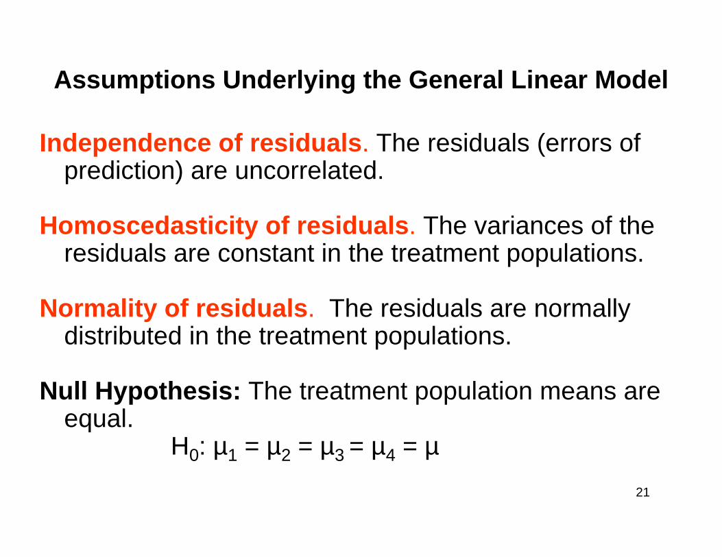
Independence of residuals. The residuals (errors of prediction) are uncorrelated.
Homoscedasticity of residuals. The variances of the residuals are constant in the treatment populations.
Normality of residuals. The residuals are normally distributed in the treatment populations.
Null Hypothesis: The treatment population means areequal.
H0: µ1 = µ2 = µ3 = µ4 = µ
Assumptions Underlying the General Linear Model
22
References
Cohen, J. (1968). Multiple regression as a general data-analytic system. Psychological Bulletin, 70,426-443.
Cohen, J. & Cohen, P. (1983). Applied Multiple Regression/Correlation Analysis for the Behavioral Sciences (Second Edition). Hillsdale, NJ: Lawrence Erlbaum.
Cohen, J., Cohen, P., West, S.G., & Aiken, L.S. (2003). Applied Multiple Regression/Correlation Analysis for the Behavioral Sciences (Third Edition). Hillsdale, NJ: Lawrence Erlbaum.