NEURO M203 & BIOMED M263 WINTER 2014

MRI Lab 1: Structural and Functional Anatomy

During today’s lab, you will work with and view the structural and functional imaging data collected from the scanning session you participated in earlier this quarter. If you did not receive a brain scan, you will work with the test dataset.

If possible, please download the software (Brainsuite) and data to your laptop before coming to lab. If you do not have a laptop to work with, you may use one of the computers in the wet lab. However, since these desktop computers have different system configurations, it is better to use your own laptop if you can.

Instructions For Downloading Imaging Software And Data

Downloading Software

• BrainSuite is an MRI processing, analysis and visualization tool developed at UCLA

1. To install BrainSuite, you will need to first register (http://brainsuite.org/register/) for a free account, after which you can download (http://brainsuite.org/download/) the latest version of the software.

2. Please follow the installation instructions on this page: http://brainsuite.bmap.ucla.edu/quickstart/installation/

3. Your computer should be running either 64-bit Windows or Mac OS X (10.6 or greater).

Downloading Data

1. Open a browser, go to http://users.bmap.ucla.edu/~narr/M203_NEUROANATOMY_LAB/ and find the zipped folder that contains your imaging data. Your folder can be identified by your initials and the date you were scanned in Feb (i.e., folders are named M203_[YOUR INITIALS]_[DAY AND YEAR OF SCAN]. Download this folder.

2. If you did not receive a brain scan, download the sample dataset, which is in a folder named M203_SAMPLE_1314.

3. Download the files named group_fmri_zstat1.nii.gz and Structural_Atlas.nii.gz, which contains the average activation map from the class and structural atlas.

4. Unzip your folder on your computer desktop. This will take many megabytes of space.

*Note: Please do not download folders of other students. Since system software is not the same on all the wet lab computers, it is possible you may have problems downloading. Let us know and we will upload your data from a flash drive.

Imaging Data

1. You should see the following files in your own folder (or the folder of the sample subject):

a. *!ANGIO.nii.gz (angiography scan)

b. *PD.nii.gz (Proton Density scan)

c. *mprage.nii.gz (T1-weighted scan)

d. *T1_masked.nii.gz

e. *svreg.label.nii.gz (BrainSuite generated subcortical labels)

f. *aparc+aseg.nii.gz (Freesurfer generated cortical labels)

g. *T2.nii.gz (T2-weighted scan)

h. *left.pial.cortex.svreg.dfs (left hemisphere surface)

i. *right.pial.cortex.svreg.dfs (right hemisphere surface)

j. zstat1.nii.gz (single subject activation map)

k. example_func.nii.gz

2. You should also have the following two files:

a. group_fmri_zstat1.nii.gz (average activation map)

b. Structural_Atlas.nii.gz

Overview Exercises

The plan for viewing your imaging data is as follows (instructions for each step are provided below):

1. After downloading BrainSuite and your data, we will begin by loading your T1-weighted structural imaging data. You will be able to view the images of your brain in each of the 3 major viewing planes so that you can identify different cortical and subcortical structures.

2. While the T1 image is still loaded, you will also load:

a. The files that will allow you to see the surface structure of your cortex in 3D

b. You will then add a file that contains color-coded labels of brain regions to superimpose onto the T1 image. These labels have been generated automatically

so the boundaries might not be exact, but you can see how you were able to correctly identify different brain regions.

3. After viewing your T1 data you will close Brainsuite and reopen it to load and view the T2-weighted and proton density weighted images of your brain, each separately. This will allow you to see different types of contrast used for MRI.

4. After again closing the program and reopening it, you will load the angiography slab into Brainsuite. You should be able to see the Circle of Willis. Note, this image is not a 3D volume, so you will not be able to scroll through in all viewing planes it as you did for the other images.

5. After again closing and reopening BrainSuite, you will view the activation maps for the finger tapping experiment you performed in the scanner. Since these maps represent activation from a single subject only, they may look noisy, but you should still see concentrated patterns of activation in sensorimotor areas.

6. After viewing your individual activation maps, you will close and reopen BrainSuite to view the average activation map from all students that performed the fMRI experiment. You will notice that the patterns of activation are more localized.

7. Next, you will reload your T1 data and will run some image processing steps that will allow you to remove extra-cortical tissue from your brain and segment your brain into different regions.

8. You are welcome to keep your data for your own use. However, please don’t copy anyone else’s data.

*Note we can direct you to other image analysis programs for use outside the lab if you are interested.

!

!

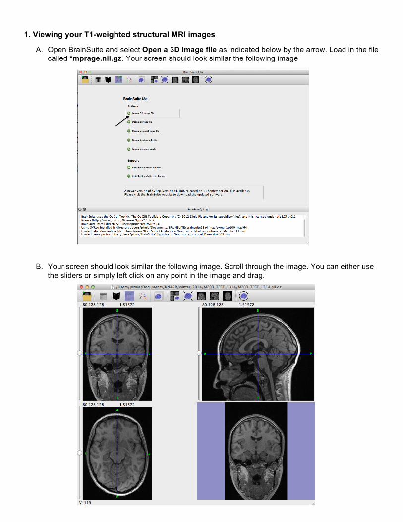
1. Viewing your T1-weighted structural MRI images

A. Open BrainSuite and select Open a 3D image file as indicated below by the arrow. Load in the file called *mprage.nii.gz. Your screen should look similar the following image

B. Your screen should look similar the following image. Scroll through the image. You can either use the sliders or simply left click on any point in the image and drag.

!

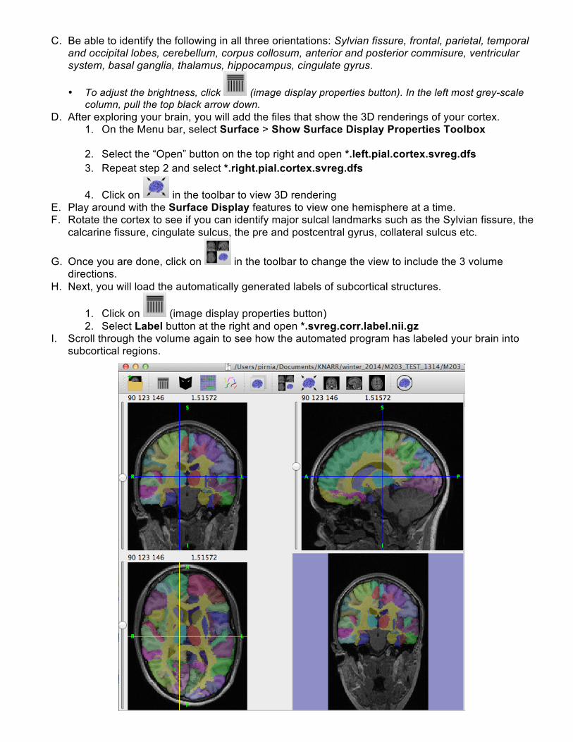
C. Be able to identify the following in all three orientations: Sylvian fissure, frontal, parietal, temporal and occipital lobes, cerebellum, corpus collosum, anterior and posterior commisure, ventricular system, basal ganglia, thalamus, hippocampus, cingulate gyrus.

• To adjust the brightness, click (image display properties button). In the left most grey-scale column, pull the top black arrow down.

D. After exploring your brain, you will add the files that show the 3D renderings of your cortex. 1. On the Menu bar, select Surface > Show Surface Display Properties Toolbox

2. Select the “Open” button on the top right and open *.left.pial.cortex.svreg.dfs 3. Repeat step 2 and select *.right.pial.cortex.svreg.dfs

4. Click on in the toolbar to view 3D rendering E. Play around with the Surface Display features to view one hemisphere at a time. F. Rotate the cortex to see if you can identify major sulcal landmarks such as the Sylvian fissure, the

calcarine fissure, cingulate sulcus, the pre and postcentral gyrus, collateral sulcus etc.

G. Once you are done, click on in the toolbar to change the view to include the 3 volume directions.

H. Next, you will load the automatically generated labels of subcortical structures.

1. Click on (image display properties button) 2. Select Label button at the right and open *.svreg.corr.label.nii.gz

I. Scroll through the volume again to see how the automated program has labeled your brain into subcortical regions.

!

J. Close the BrainSuite generated label (*.svreg.corr.label.nii.gz) by selecting the X next to the Label in the Image Display side bar.

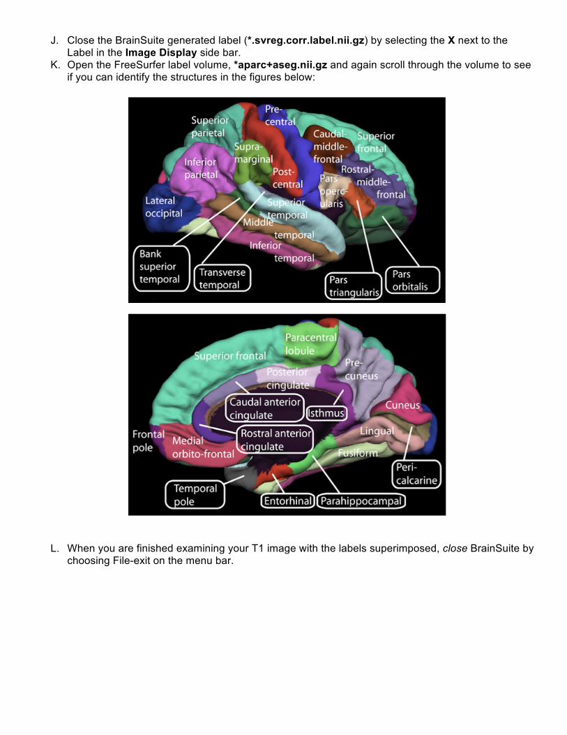
K. Open the FreeSurfer label volume, *aparc+aseg.nii.gz and again scroll through the volume to see if you can identify the structures in the figures below:

L. When you are finished examining your T1 image with the labels superimposed, close BrainSuite by choosing File-exit on the menu bar.

!

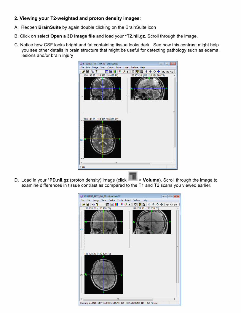
2. Viewing your T2-weighted and proton density images:

A. Reopen BrainSuite by again double clicking on the BrainSuite icon

B. Click on select Open a 3D image file and load your *T2.nii.gz. Scroll through the image.

C. Notice how CSF looks bright and fat containing tissue looks dark. See how this contrast might help you see other details in brain structure that might be useful for detecting pathology such as edema, lesions and/or brain injury

D. Load in your *PD.nii.gz (proton density) image (click > Volume). Scroll through the image to examine differences in tissue contrast as compared to the T1 and T2 scans you viewed earlier.

!

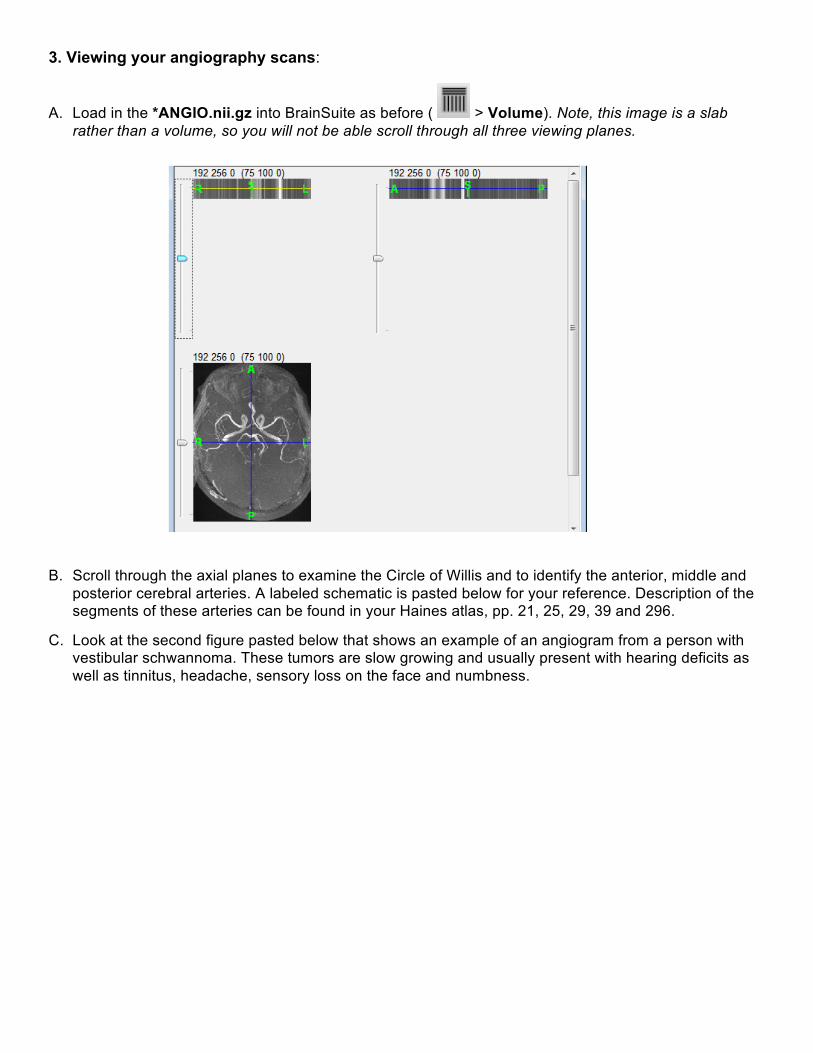
3. Viewing your angiography scans:

A. Load in the *ANGIO.nii.gz into BrainSuite as before ( > Volume). Note, this image is a slab rather than a volume, so you will not be able scroll through all three viewing planes.

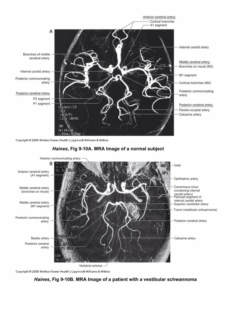
B. Scroll through the axial planes to examine the Circle of Willis and to identify the anterior, middle and posterior cerebral arteries. A labeled schematic is pasted below for your reference. Description of the segments of these arteries can be found in your Haines atlas, pp. 21, 25, 29, 39 and 296.

C. Look at the second figure pasted below that shows an example of an angiogram from a person with vestibular schwannoma. These tumors are slow growing and usually present with hearing deficits as well as tinnitus, headache, sensory loss on the face and numbness.

!

Haines, Fig 9-10A. MRA Image of a normal subject!

Haines, Fig 9-10B. MRA Image of a patient with a vestibular schwannoma!

!

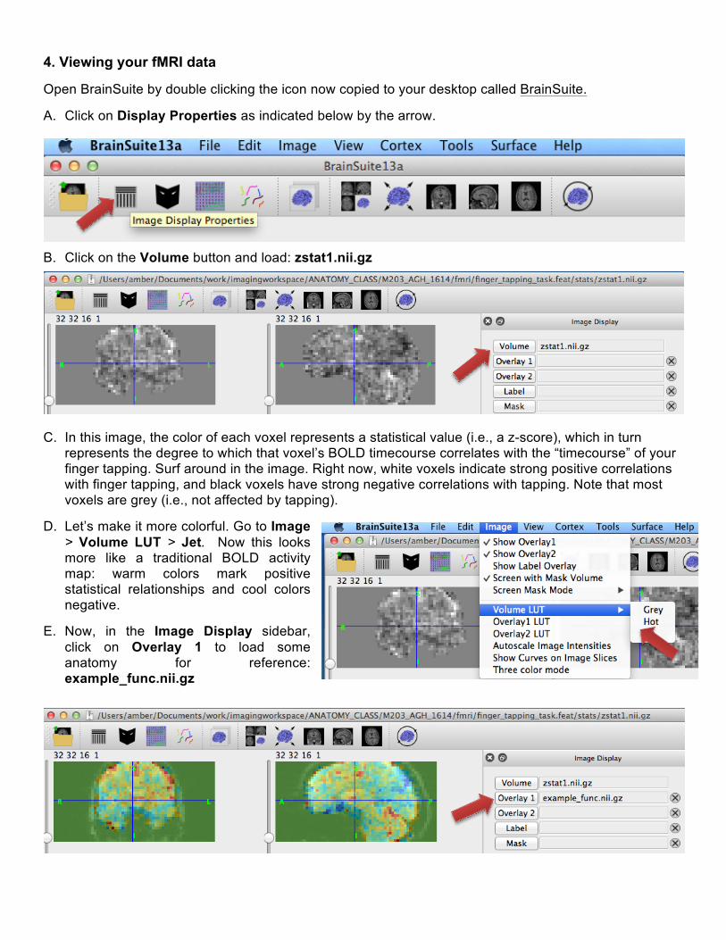
4. Viewing your fMRI data

Open BrainSuite by double clicking the icon now copied to your desktop called BrainSuite.

A. Click on Display Properties as indicated below by the arrow.!

B. Click on the Volume button and load: zstat1.nii.gz !

C. In this image, the color of each voxel represents a statistical value (i.e., a z-score), which in turn represents the degree to which that voxel’s BOLD timecourse correlates with the “timecourse” of your finger tapping. Surf around in the image. Right now, white voxels indicate strong positive correlations with finger tapping, and black voxels have strong negative correlations with tapping. Note that most voxels are grey (i.e., not affected by tapping).!!

D. Let’s make it more colorful. Go to Image > Volume LUT > Jet. Now this looks more like a traditional BOLD activity map: warm colors mark positive statistical relationships and cool colors negative.!

E. Now, in the Image Display sidebar, click on Overlay 1 to load some anatomy for reference: example_func.nii.gz

!

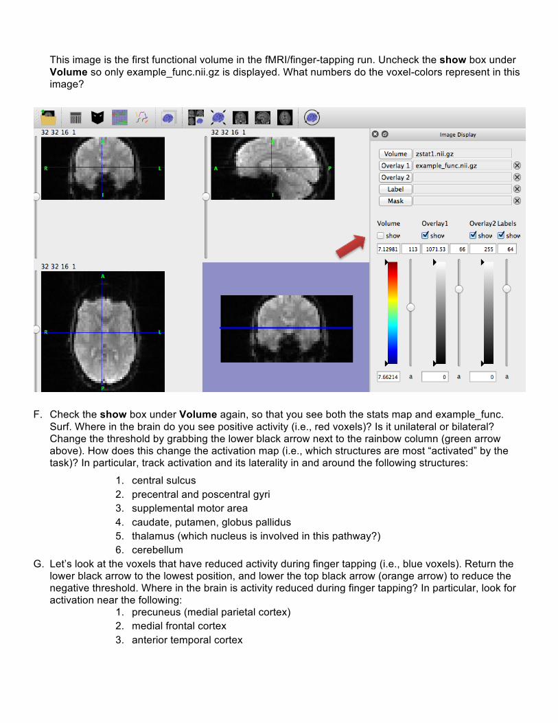
This image is the first functional volume in the fMRI/finger-tapping run. Uncheck the show box under Volume so only example_func.nii.gz is displayed. What numbers do the voxel-colors represent in this image?

F. Check the show box under Volume again, so that you see both the stats map and example_func. Surf. Where in the brain do you see positive activity (i.e., red voxels)? Is it unilateral or bilateral? Change the threshold by grabbing the lower black arrow next to the rainbow column (green arrow above). How does this change the activation map (i.e., which structures are most “activated” by the task)? In particular, track activation and its laterality in and around the following structures:

1. central sulcus 2. precentral and poscentral gyri 3. supplemental motor area 4. caudate, putamen, globus pallidus 5. thalamus (which nucleus is involved in this pathway?) 6. cerebellum

G. Let’s look at the voxels that have reduced activity during finger tapping (i.e., blue voxels). Return the lower black arrow to the lowest position, and lower the top black arrow (orange arrow) to reduce the negative threshold. Where in the brain is activity reduced during finger tapping? In particular, look for activation near the following:

1. precuneus (medial parietal cortex) 2. medial frontal cortex 3. anterior temporal cortex

!

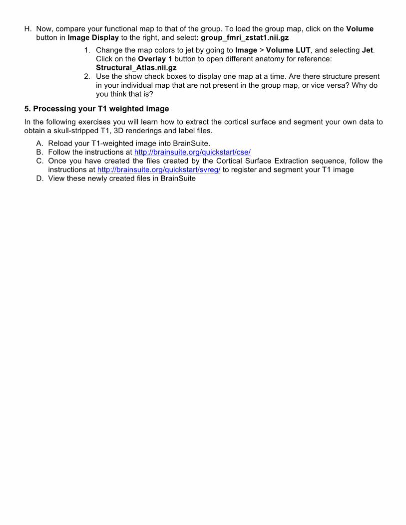
H. Now, compare your functional map to that of the group. To load the group map, click on the Volume button in Image Display to the right, and select: group_fmri_zstat1.nii.gz

1. Change the map colors to jet by going to Image > Volume LUT, and selecting Jet. Click on the Overlay 1 button to open different anatomy for reference: Structural_Atlas.nii.gz

2. Use the show check boxes to display one map at a time. Are there structure present in your individual map that are not present in the group map, or vice versa? Why do you think that is?

5. Processing your T1 weighted image In the following exercises you will learn how to extract the cortical surface and segment your own data to obtain a skull-stripped T1, 3D renderings and label files.

A. Reload your T1-weighted image into BrainSuite. B. Follow the instructions at http://brainsuite.org/quickstart/cse/ C. Once you have created the files created by the Cortical Surface Extraction sequence, follow the

instructions at http://brainsuite.org/quickstart/svreg/ to register and segment your T1 image D. View these newly created files in BrainSuite