•IM •Controller •SM •Prime •Mover •SM •Prime •Mover •Other electrical •consumptions •Pulsed Power •for EM Gun •Pulsed Power •for EM Gun •IM •Controller Multi-Element Generalized Polynomial Chaos: A New Method to Model Uncertainty in Complex Systems P. Prempraneerach, X. Wan and G.E Karniadakis MIT and Brown University •Instead of relying on operational safety margins – which we hope are sufficiently conservative – an operational decision can be based on the probability of exceeding a set of specified limits. New Simulation Approach:
Transcript
•IM •Controller
•SM •Prime
•Mover
•SM •Prime
•Mover
•Other electrical
•consumptions
•Pulsed Power
•for EM Gun
•Pulsed Power
•for EM Gun
•IM •Controller
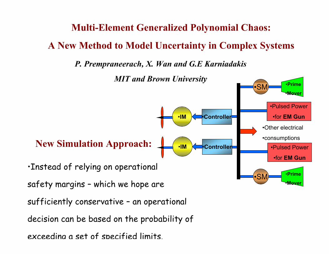
Multi-Element Generalized Polynomial Chaos:
A New Method to Model Uncertainty in Complex Systems
P. Prempraneerach, X. Wan and G.E Karniadakis
MIT and Brown University
•Instead of relying on operational
safety margins – which we hope are
sufficiently conservative – an operational
decision can be based on the probability of
exceeding a set of specified limits.
New Simulation Approach:
Bus#1: 3-phaseradial system
Prime Mover 1(Gas Turbine)
Governor
SM1
Exciter I_
IM1
IM2
Bus#2: 3-phaseradial system
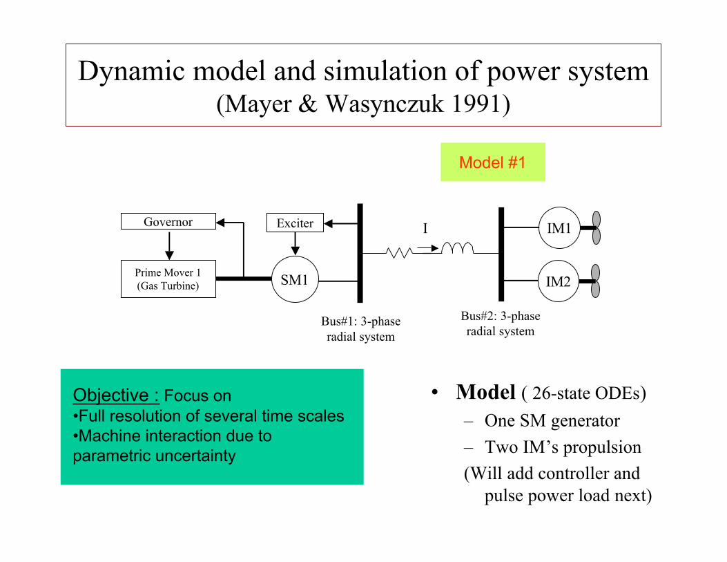
Model #1
Dynamic model and simulation of power system(Mayer & Wasynczuk 1991)
Objective : Focus on•Full resolution of several time scales•Machine interaction due toparametric uncertainty
• Model ( 26-state ODEs)– One SM generator
– Two IM’s propulsion
(Will add controller andpulse power load next)
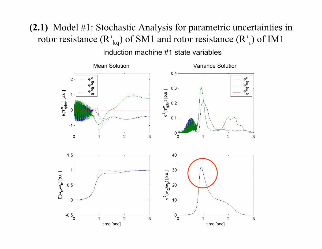
Induction machine #1 state variables
Variance SolutionMean Solution
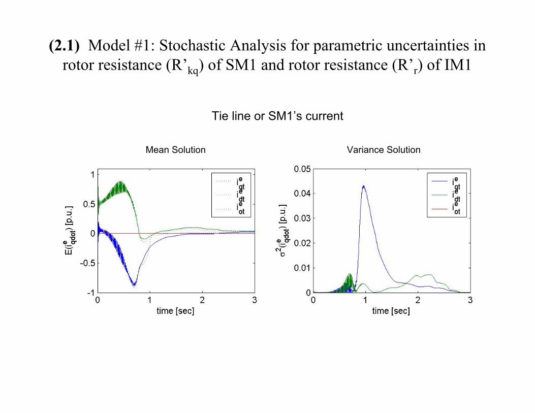
(2.1) Model #1: Stochastic Analysis for parametric uncertainties inrotor resistance (R’kq) of SM1 and rotor resistance (R’r) of IM1
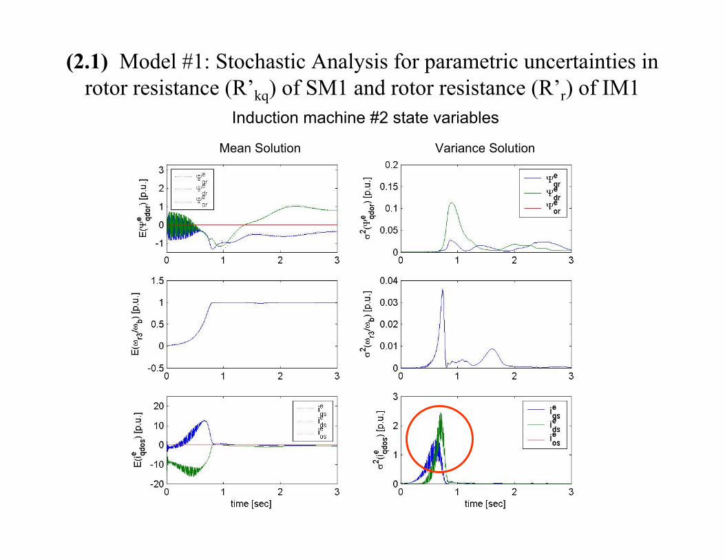
Induction machine #2 state variables
Variance SolutionMean Solution
(2.1) Model #1: Stochastic Analysis for parametric uncertainties inrotor resistance (R’kq) of SM1 and rotor resistance (R’r) of IM1
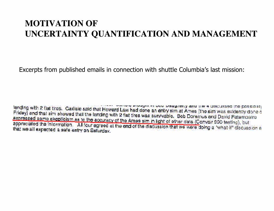
Excerpts from published emails in connection with shuttle Columbia’s last mission:
MOTIVATION OFMOTIVATION OFUNCERTAINTY QUANTIFICATION AND MANAGEMENTUNCERTAINTY QUANTIFICATION AND MANAGEMENT
(Years: 1999,’94,’90,’88,’84,’78,’72)– Less in transient stability, almost nothing in parametric uncertainties– Reference: PhD Thesis, MIT (2000), J.R. Hockberry “Evaluation of
uncertainty in dynamic, reduced-order power system models”
• Sources of Uncertainty:– Load models, fault time, frequency, angle and voltage variations,
Stochastic Modeling:- Stochastic differential-algebraic equations (need fast methods)- More efficient parameter-space exploration- Sensitivity/reliability studies- Comparisons with experiments is more meaningful
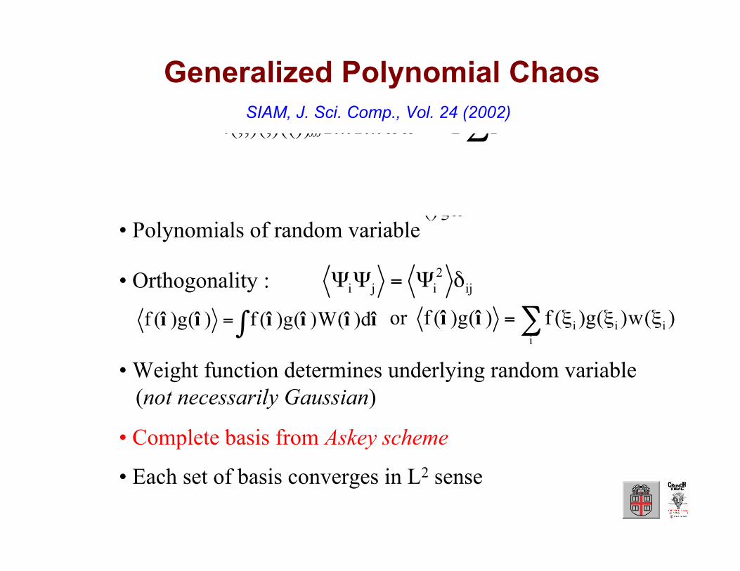
Generalized Polynomial ChaosSIAM, J. Sci. Comp., Vol. 24 (2002)
0(,;)(,)(())jjjTxtTxtωω∞==Ψ∑î
• Orthogonality : ij2iji δΨ=ΨΨ
∫= îîîîîî d)(W)(g)(f)(g)(f
• Weight function determines underlying random variable (not necessarily Gaussian)
• Complete basis from Askey scheme
• Polynomials of random variable()ξω
• Each set of basis converges in L2 sense
∑ ξξξ=i
iii )(w)(g)(f)(g)(f or îî
The Askey Scheme
)0(F02
)1(F02)1(F11
)2(F12
)3(F23
)4(F34
Wiener, Ghanem & Spanos
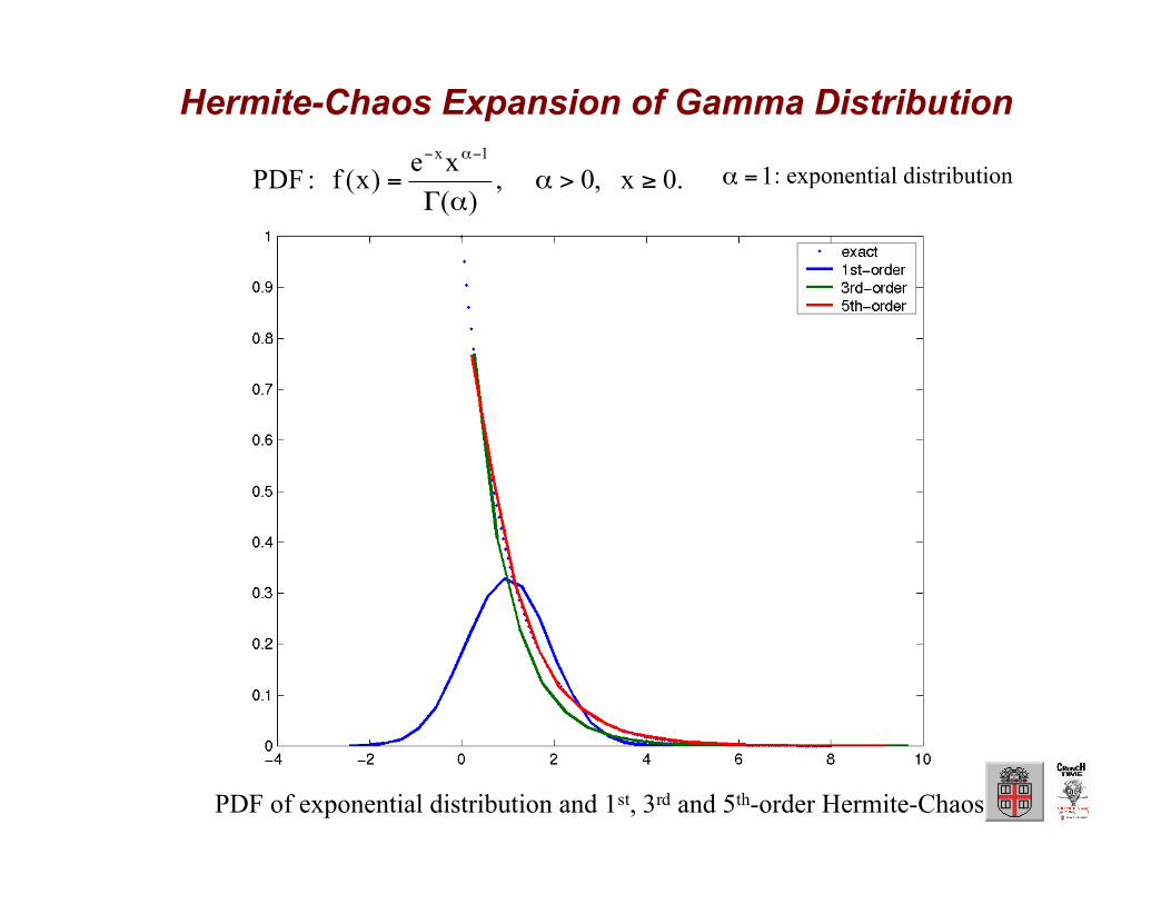
Hermite-Chaos Expansion of Gamma Distribution
PDF of exponential distribution and 1st, 3rd and 5th-order Hermite-Chaos
.0x ,0 ,)(
xe)x(f :PDF
1x
≥>ααΓ
=−α−
1=α : exponential distribution
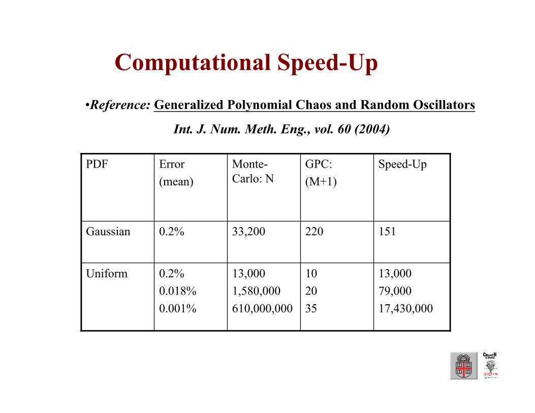
13,000
79,000
17,430,000
10
20
35
13,000
1,580,000
610,000,000
0.2%
0.018%
0.001%
Uniform
15122033,2000.2%Gaussian
Speed-UpGPC:
(M+1)
Monte-Carlo: N
Error
(mean)
PDF
Computational Speed-Up
•Reference: Generalized Polynomial Chaos and Random Oscillators
Int. J. Num. Meth. Eng., vol. 60 (2004)
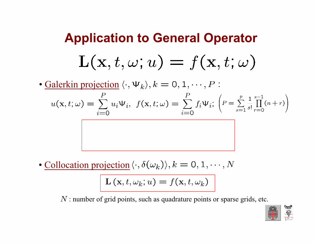
Application to General Operator
• Galerkin projection
• Collocation projection
: number of grid points, such as quadrature points or sparse grids, etc.
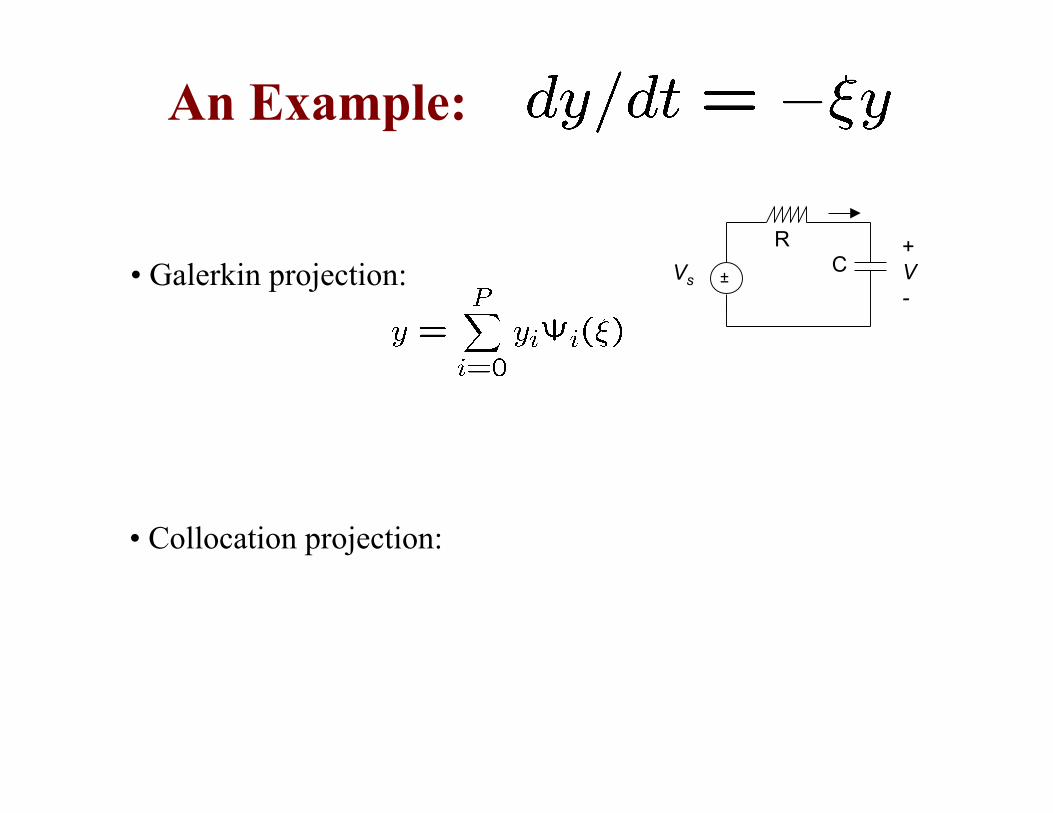
An Example:
• Galerkin projection:
• Collocation projection:
±
+V-
CR
Vs
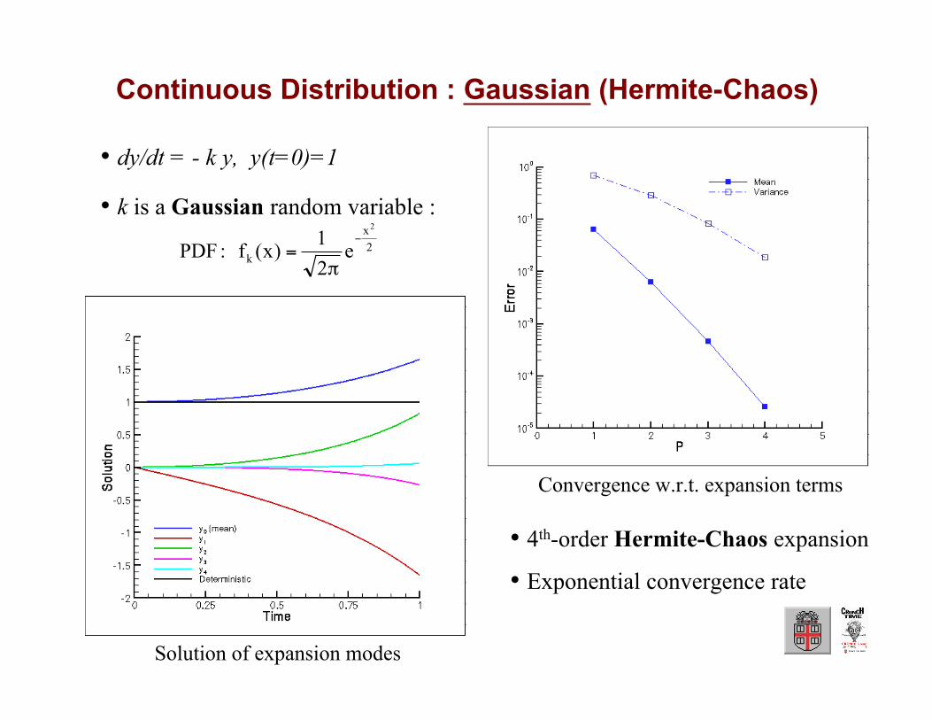
Continuous Distribution : Gaussian (Hermite-Chaos)
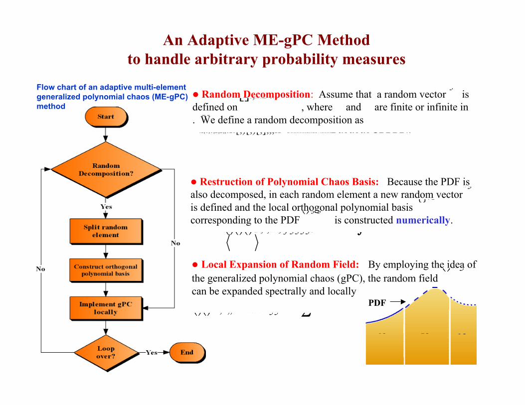
Random Decomposition: Assume that a random vector isdefined on , where and are finite or infinite in. We define a random decomposition as
ia ib[]1,diiiBab==×ξ
R
Restruction of Polynomial Chaos Basis: Because the PDF isalso decomposed, in each random element a new random vectoris defined and the local orthogonal polynomial basiscorresponding to the PDF is constructed numerically.
kξ
()kfξ{}iΦ
()()()dkijikjkkkijBfξξξξδΦΦ=ΦΦ=∫
Flow chart of an adaptive multi-elementgeneralized polynomial chaos (ME-gPC)method
Local Expansion of Random Field: By employing the idea ofthe generalized polynomial chaos (gPC), the random fieldcan be expanded spectrally and locally
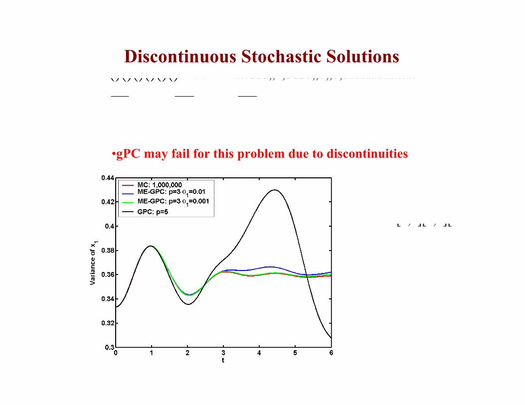
•gPC may fail for this problem due to discontinuities
101202303[1,1][1,1][1,1]xUxUxUξξξ=∈−=∈−=∈−
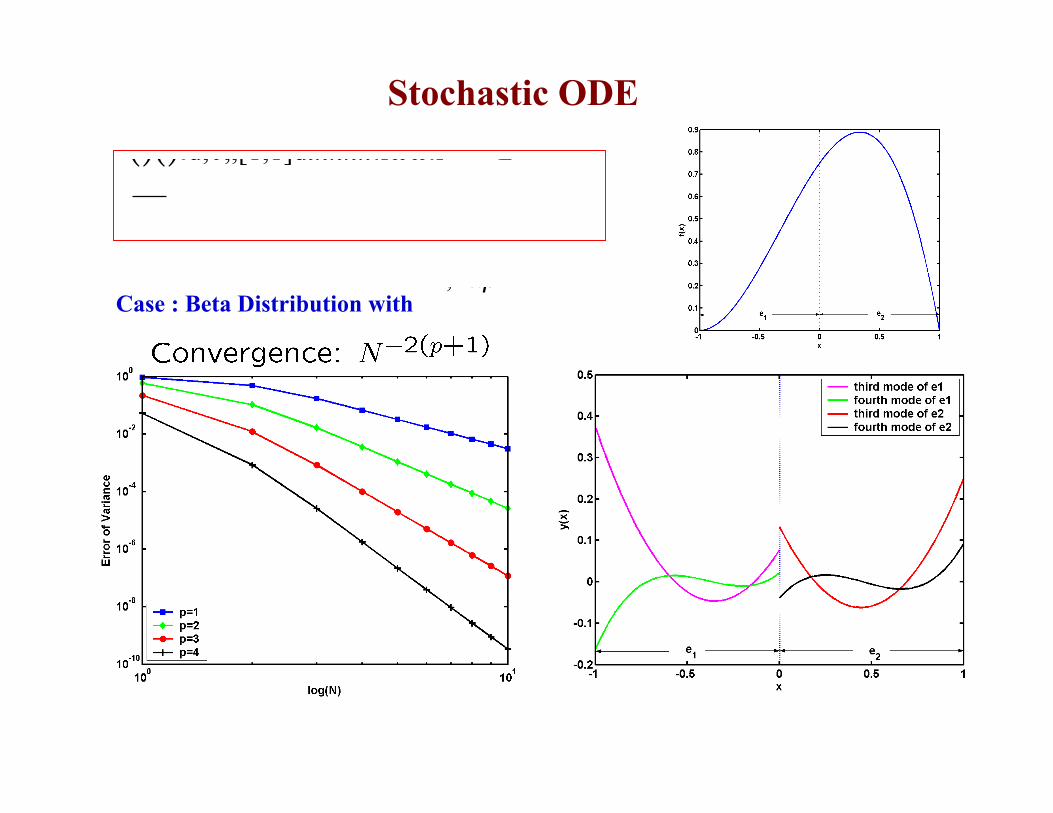
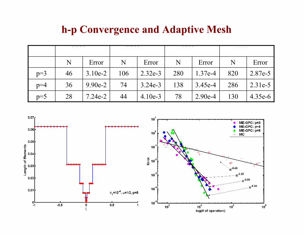
h-p Convergence and Adaptive Mesh
4.35e-61302.90e-4784.10e-3447.24e-228p=5
2.31e-52863.45e-41383.24e-3749.90e-236p=4
2.87e-58201.37e-42802.32e-31063.10e-246p=3
ErrorNErrorNErrorNErrorN
2110θ−= 4110θ−=3110θ−= 5110θ−=
(c): t=6
(b): t=3
(a): t=1
2D Adaptive Mesh for Discontinuous Solutions
Problem:
An accuracy of O(10-4) is maintained by adaptive meshes.
The elements are well refined around the discontinuous region ξ1=0.
The number of random elements increases almost linearly with time.
gPC fails to converge after a short-term integration.
Tie line or SM1’s current
Variance SolutionMean Solution
(2.1) Model #1: Stochastic Analysis for parametric uncertainties inrotor resistance (R’kq) of SM1 and rotor resistance (R’r) of IM1
•D. Xiu and G.E. Karniadakis, “The Wiener-Askey polynomial chaos for stochastic differentialequations”, SIAM J. Sci. Comput., vol. 24(2), pp. 619-644, 2002.
•D. Xiu and G.E. Karniadakis, “Modeling uncertainty in flow simulations via GeneralizedPolynomial Chaos”, J. Comp. Phys., vol. 87, pp. 137-167, 2003.
• D. Xiu and G.E. Karniadakis, “Modeling uncertainty in steady state diffusion problems viaGeneralized Polynomial Chaos”, Comput. Meth. Appl. Mech. Eng., vol 191, pp. 4927-4948, 2002.
• D. Lucor and G.E. Karniadakis, “Adaptive generalized polynomial chaos for nonlinear randomoscillators", SIAM J. Sci. Comput., vol. 26(2), pp. 720-735, 2004.
• X. Wan and G.E. Karniadakis, “An adaptive multi-element generalized polynomial chaosmethod for stochastic differential equations", J. Comp. Phys., vol. 209(2), pp. 617-642, 2005.
•X. Wan and G.E. Karniadakis, “Beyond Wiener-Askey expansions: Handling arbitrary PDFs",
Journal of Scientific Computing, in press.
•X. Wan and G.E. Karniadakis, “Multi-element generalized polynomial chaos for arbitraryprobability measures”, SIAM J. Sci. Comput., in press, 2006.
•X. Wan and G.E. Karniadakis, “Long-term behavior of polynomial chaos in stochastic flowsimulations", Comput. Methods Appl. Mech. Engrg., in press, 2006.
References on Stochastic Modeling
Comparison of Cost between MC and ME-gPC
Only h-convergence, N-2(p+1), is considered. N is the random element number along onerandom dimension and p is the polynomial chaos order.
For the same accuracy and different random dimension numbers, the lines show thecases where the cost of standard Monte Carlo is equal to that of ME-gPC. For a certainrandom dimension number, the region below the line is where MC wins; the region abovethe line is where ME-gPC wins.