Yadav et al., Cogent Engineering (2016), 3: 1272159http://dx.doi.org/10.1080/23311916.2016.1272159
PRODUCTION & MANUFACTURING | RESEARCH ARTICLE
Multi-item multi-constraint supply chain integrated inventory model with multi-variable demand under the effect of preservation technologyDharmendra Yadav1*, S.R. Singh2 and Vandana Arora3
Abstract: Today’s every firms have realized that managing supply chain (SC) and deciding their integrated scheduling policy is substantial. Decision-makers of all the firms always keep searching different policies such as trade credit, preservation tech-nology. By adopting these policies they help in strengthen the relationship among different players of supply chain. It is also observed that decision-makers develop policies for integrated system under some restrictions such as budget constraint. Infeasible solutions of many real world problems are obtained by ignoring such restriction. On focusing all these issues, in this paper, a multi-item integrated sup-ply chain inventory model is formulated by considering one manufacturer and one retailer over a finite planning horizon. Manufacturer provides trade credit period to its retailer to strengthen the supply chain. It is assumed that the demand is multi-vari-able which depends on trade credit period and selling price of the items. In a real-life integrated supply chain inventory system, limitations on available budget and storage space are always faced by the manufacturer and the retailer. So, model is formulated to minimize the total integrated cost of the system subject to space and budget constraints. Optimal values of decision variables and objective function is obtained by using Lagrangian Multiplier Method (LMM). Proposed model is illustrated with the help of numerical and sensitive analysis is carried out with respect to different parameters.
Subjects: Mathematical Modeling; Operations Research; Production Research & Economics
Keywords: integrated model; multi-variable demand; budget and space constraint; trade credit; Lagrangian multiplier method
*Corresponding author: Dharmendra Yadav, Department of Mathematics, Vardhaman (P.G.) College, Bijnor 246701, Uttar Pradesh, India E-mail: [email protected]
Reviewing editor:Yibing Li, Wuhan University of Technology, China
Additional information is available at the end of the article
ABOUT THE AUTHORDharmendra Yadav is an assistant professor in Vardhaman (P.G.) College, MJP Rohilkhand University, Bijnor, U.P. (India). He received his PhD in Inventory Control from the CCS University. His interests are in operations and supply chain management and optimization. He has had his articles published in journals, such as Opsearch, Asia-Pacific Journal of Operational Research, International Journal of Systems Science, International Journal of Operational Research, and others.
PUBLIC INTEREST STATEMENTAim of this paper is to develop a multi-item integrated supply chain inventory model by considering one manufacturer and one retailer over a finite planning horizon. Manufacturer provides trade credit period to its retailer to strengthen the supply chain. It is assumed that the demand is multi-variable which depends on trade credit period and selling price of the items. In practical situation, limitations on available budget and storage space are always faced by the manufacturer and the retailer. So, model is formulated to minimize the total integrated cost of the system subject to space and budget constraints.
Received: 15 July 2016Accepted: 11 December 2016First Published: 29 December 2016
Yadav et al., Cogent Engineering (2016), 3: 1272159http://dx.doi.org/10.1080/23311916.2016.1272159
1. IntroductionNow-a-days, people try to utilize their maximum time to manage their professional life and their target is to invest minimum time for each and every non professional work. Therefore, everyone prefers to shop for their necessary commodities in a single roof and save their time. Due to this, importance of shopping mall or a supermarket type retailing shop in modern civilization is increasing slowly but surely with the passage of time. Its basic appeal is the availability of variety of goods under a single roof. Consequently, manufacturing and marketing policies are also changed with time. Manufacturer of different industries like electrical goods industries, food product industries, automobile industries etc. not focused to manufacturer only single item but their target is to manu-facture multi-item under a single roof. Now, it is a big challenge to the inventory practitioners and researchers to coordinate multi-item manufacturing industry and retailing shops in a supply chain. Inventory practitioners also start practicing in the direction that when retailer/manufacturer of a factory starts the business/manufacturing has a fixed budget to purchase the items and a godown of finite area to store the items.
Miller (1971) proposed a mathematical model to control multi-item inventory problem with back-order where the objective function is to minimize subjected to a budget constraint. Page and Paul (1976) formulated the basic lot size inventory problem when there was a multi-item for which inven-tories must be maintained. They optimized their objective function subjected to the space con-straints and budget constraints. Rosenblatt and Rothblum (1990) developed mathematical model for multi-item inventory problem subjected to a single resource capacity constraints where the ca-pacity of storage space was considered as decision variables. Das, Roy, and Maiti (2000) formulated a fully backlogged multi-item inventory model with constant demand subjected to storage area, total average inventory investment cost and total average shortage cost. They considered that in-ventory costs are directly proportional to the respective quantities and the unit production cost is inversely related to the demand. Das, Roy, and Maiti (2004) formulated fully backlogged stochastic and fuzzy-stochastic multi-item inventory problems with demand dependent unit cost under stor-age-space and budgetary constraints. They assumed that inventory costs were dependent on their respective quantities. They considered demand and both the resources i.e. budgetary amount and storage area as random variable for the stochastic model. Maity and Maiti (2007) developed a math-ematical model for multi-item dynamic production-inventory control problem. They obtained the optimal values of objective function subjected to the imprecise budget and storage capacity con-straints which are of possibility and/or necessity types respectively. Guchhait, Maiti, and Maiti (2010) proposed a multi-item inventory model of breakable items with stock dependent demand. They considered that breakability rates increases nonlinearly with time and linearly with stock. Mandal, Maity, Maity, Mondal, and Maiti (2011) first time proposed a stock dependent multi-item multi-period production problem without and with the preparation time for a fixed time horizon. They considered holding and shortage costs and available space as fuzzy-random parameters. They solved the prob-lem by using GA. Pal, Sana, and Chaudhuri (2012) studied a multi-item deterministic economic order quantity model for a vendor when the demand rate increase exponentially with increasing level of price break and decreases quadratically with increasing sales price. They considered that when the revenue of the vendor crosses the level of price break, price discount is offered to the customers. Jana, Das, and Maiti (2014) developed partially backlogged multi-item inventory models for deterio-rating items in a random planning horizon with exponential distribution under the effect of inflation and time value money with budget and space constraints. They assumed that the demand rate de-pends on the stock. They developed two models. In first they considered that inventory parameters other than planning horizon are deterministic while in the other deterioration and net value of the money are fuzzy, available budget and space are fuzzy and random fuzzy respectively. Saha, Kar, and Maiti (2015) developed a fuzzy-stochastic multi-item multi-objective supply chain models hav-ing budget and risk constraints for long-term contract with a profit sharing scheme. They assumed that the demands of the items were random at each period and the manufacturing costs of the items were fuzzy. To reduce the multi-objective problems into corresponding single objective prob-lems, they used fuzzy compromise programming method, global criteria method and weighted sum method. Nia, Farb, and Niaki (2015) proposed a multi-item economic order quantity model with
Page 3 of 23
Yadav et al., Cogent Engineering (2016), 3: 1272159http://dx.doi.org/10.1080/23311916.2016.1272159
shortage for a single-supplier single-buyer supply chain under green vendor managed inventory (VMI) policy. They explicitly included the VMI contractual agreement between the vendor and the buyer such as warehouse capacity and delivery constraints, bounds for each order, and limits on the number of pallets. Topan, Bayındır, and Tan (2017) considered a multi-item two-echelon inventory system. They considered that central warehouse operates under a (Q, R) policy and local warehouses operates (S−1, S) policy. The objective of this study was to find the policy parameters minimizing system-wide inventory holding and fixed ordering under to aggregate and individual response time constraints.
Traditionally, integrated supply chain inventory models (ISCIM) are developed in infinite planning horizon because it is assumed that during the course of planning including the various inventory parameters, demand, etc. remain unchanged over the future infinite time. In practice, it is not so due to several reasons such as variation in inventory costs, changes in item specifications and designs, technological changes due to environmental conditions, availability of item, etc. Moreover, for sea-sonal products like warm garments, fruits, etc. business period is finite. Das, Kar, Roy, and Kar (2012) supported this idea.
In practical situation, manufacturer offer a trade credit period to retailers to settle outstanding amount of the purchasing costs to boost the demand of their products. During trade credit period, the retailer can earn interest from selling items; otherwise, the retailer has to pay interest to the manufacturer for late payment. This policy reduces the purchasing cost of the retailer indirectly and motivates the retailer to buy more. Jaber and Osman (2006) proposed a two level supply chain coor-dination approach in order to minimize the cost of the system, by incorporating a permissible delay in the payment strategy. Kin Chan, Lee, and Goyal (2010) developed an integrated single-vendor and multi-buyer supply chain model. In order to integrate the system they synchronizing the ordering and production cycles, where delayed payments based on the buyers’ ordering intervals. Tsao (2011) determined the optimal ordering and pricing policy in order to maximize the profit of integrated system when the supplier offers a cash discount to a specific retailer and a credit period to another. Shastri, Singh, Yadav, and Gupta (2014) developed an inventory model for a retailer under two-level of trade credit to reflect the supply chain management. Moussawi-Haidar, Dbouk, Jaber, and Osman (2014) investigated an integrated supply chain, which comprised a capital-constrained supplier, a retailer, and a financial intermediary (bank). The objective of supply chain is to minimize the total supply chain costs while the supplier allowed a trade credit period payment to the retailer. Cárdenas-Barrón and Sana (2014) proposed an integrated supply chain (manufacturer-retailer) model that includes sales teams’ initiatives, variable procurement costs, sensitive demand, variable production rate, production lot size, and backordering where backordering occurs only at the retailer. Chakraborty, Jana, and Roy (2015) developed multi-item integrated (supplier-retailer) supply chain model with constant rate of deterioration with stock dependent demand. They considered that sup-plier’s production cost as non-linear function depending of production rate, supplier’s transportation cost (TC) as a nonlinear function of the amount of quantity ordered by retailer and retailer’s procure-ment cost exponentially depends on the trade credit period.
Deterioration is natural phenomenon that occurs for most items in the world. It means that the worth of the product gradually decreases with respect to time. However, investigation on preserva-tion technology to reduce deterioration rate has received little attention in the past years. The con-sideration of preservation technology is important due to the fact that preservation technology can reduce the deterioration rate significantly.
Deterioration of items present in inventory had been studied in the past decades (Chakraborty et al., 2015; Dye, Ouyang, & Hsieh, 2007; Lin, Tan, & Lee, 2000; Wee, 1995; Widyadana et al., 2011; Yadav, Singh, & Kumari, 2013). However, investigation on preservation technology to reduce deterio-ration rate has received little attention in the past years. Murr and Morris (1975) showed that a lower temperature will increase the storage life and decrease decay. Moreover, drying or vacuum technol-ogy are introduced to reduce the deterioration rate of medicine and foodstuff. Zauberman, Ronen,
Page 4 of 23
Yadav et al., Cogent Engineering (2016), 3: 1272159http://dx.doi.org/10.1080/23311916.2016.1272159
Akerman and Fuchs (1990) developed a method for color retention of Litchi fruits with SO2 fumiga-tion. Quyang, Wu, and Yang (2006) found that if the retailer can reduce effectively the deteriorating rate of item by improving the storage facility, the total annual relevant inventory cost will be reduced.
Incorporating the above mentioned real life phenomenon, in this paper, a multi-item integrated supply chain inventory model is formulated by considering one manufacturer and one retailer over a finite planning horizon. Here, unit manufacturing cost, directly proportional to the corresponding raw material cost, development cost due to the system’s reliability and labour, energy, cost of tech-nology, design, complexity, resources etc. The development costs and wear-tear costs are inversely and directly proportional to production rate, respectively. Manufacturer provides trade credit period to its retailer to strengthen the supply chain. It is assumed that the demand is multi-variable which depends on trade credit period and selling price of the items. Demand is increasing function with respect to trade credit period and decreasing with respect to selling price of items. In a real-life inte-grated supply chain inventory system, limitations on available budget and storage space are always faced by the manufacturer and the retailer. So, model is formulated to minimize the total integrated cost of the system subject to space and budget constraints. Optimal values of decision variables and objective function is obtained by using Lagrangian Multiplier Method (LMM).
2. Assumptions and notations
2.1. AssumptionThe mathematical model developed in this paper is based on the following assumptions:
(1) Consider a supply chain in which a manufacturer produces ‘n’ different items and distributes to a retailer.
(2) Manufacturing rate is assumed to be greater than the demand rate.
(3) In this manufacturing-inventory system the whole business period is assumed to be finite.
(4) The replenishment rate is infinite and there is no lead time.
(5) Shortages are not allowed.
(6) Deterioration is considered at the retailer end only.
(7) Retailer invests in the preservation technology (PT) to reduce the deterioration rate.
(8) It is assumed that the trade credit period (Mi) offered by the manufacturer must be within each replenishment period (Ti) for the ith item. This assumption is considered for the conveni-ence of mathematical representation. This assumption is practically true for the developing countries where manufacturer do not take much risk.
(9) Demand rate D(si, Mi) is the function of selling price and the credit period offered by the manu-facturer to the retailer. Demand rate is increasing function with respect of trade credit and decreasing function with respect to selling price.
(10) Retailer’s procurement cost depends on the trade credit period offered by the manufacturer.
(11) Manufacturer transportation cost depends on the order size ordered by the retailer.
(12) Unit manufacturing cost is related to the manufacturing rate.
2.2. AssumptionsFollowing notations has been used for the development of mathematical model developed in this paper:
Ari Retailer ordering cost per order for the ith item
Smi Manufacturer’s setup cost per production run for the ith item
Page 5 of 23
Yadav et al., Cogent Engineering (2016), 3: 1272159http://dx.doi.org/10.1080/23311916.2016.1272159
Pmi Manufacturing rate of the ith item
M(Pmi) Unit manufacturing cost (= Mmi +
Gmi
Pmi+ BmiP
�i
mi
) Mmi
(> 0
) is the cost compo-
nent includes the raw material cost and independent of manufacturing rate Gmi
Pmi
(Gmi , Pmi > 0
) is the cost component per unit item that decreases with in-
crease of manufacturing rate BmiP𝛾i
mi
(Bmi , Pmi > 0
) is the cost component per
unit item that increases with Increase of manufacturing rate
Cri Retailer’s procurement cost for the ith item (= C0ri + C
1rie
Mi
),C1ri > 0 where C0ri is
the procurement cost in the absence of trade credit period
hri Retailer’s holding cost for the ith item
hmi Manufacturer’s holding cost for the ith item
sri Retailer’s selling for the ith item
θri Deterioration rate for the ith item at the retailer end
uri The preservation technology investment per unit by the retailer’s for the ith item
fi(uri
) The proportion of reduced deterioration rate for the ith item
(0 ≤ fi
(uri
)≤ 1
)φri The subsidy proportion of preservation technology investment for the ith item
gri The cost coefficient of the investment for the ith item
Ti Replenishment time interval of the retailer in a year unit for the ith item (decision variable)
Mi Trade credit period offered by the manufacturer to the retailer’s for the ith item (decision variable)
Ici Interest charged by the manufacturer to the retailer on the outstanding inven-tory after the trade credit period Mi for each ith item
qdri Interest rest on revenue deposited by the retailer for the ith item
qdmi Interest rest to calculating manufacturer’s opportunity interest loss due to delay payment for the ith item
ni Number of replenishment of retailer for the ith item
Qi Ordering quantity by the retailer to the manufacturer in each cycle for the ith item
3. Formulation of multi-item integrated supply chain mathematical modelIn this work, a two-echelon supply chain with one manufacturer and one retailer is considered. Manufacturer producing n different items and distribute to a retailer from where customer demands are satisfied. The production period of the manufacturer starts at time t = 0 at the manufacturing rate Pmi (for ith item). At the end of the replenishment period, retailer receives the amount Qi (for the ith item) from the manufacturer. During the period of Ti, retailer satisfies the demand of the cus-tomer from the stock. At the end of period retailer again placed the order to the manufacturer of quantity Qi (for the ith item). Manufacturer again delivered the ordered quantity Qi (for the ith item) to the retailer. This process continues up to time niTi. At the end of the time (ni + 1)Ti the inventory
Page 6 of 23
Yadav et al., Cogent Engineering (2016), 3: 1272159http://dx.doi.org/10.1080/23311916.2016.1272159
level of the retailer becomes zero. The behavior of the inventory level of manufacturer and retailers is presented in Figure 1.
3.1. Formulation of retailer mathematical modelInventory level Ii(t) for the ith item for each replenishment cycle of retailer can be describe by the following differential equation:
(1)dIi(t)
dt+(1 − fi
(uri
))�riIi(t) = −Di
(si ,Mi
), 0 ≤ t ≤ Ti
Figure 1. Integrated supply chain model.
Page 7 of 23
Yadav et al., Cogent Engineering (2016), 3: 1272159http://dx.doi.org/10.1080/23311916.2016.1272159
With the boundary condition Ii(0)= Qi and Ii
(Ti)= 0.
On solving the differential Equation (1) by using the boundary condition, we get:
We have Ii(0)= Qi, so we get:
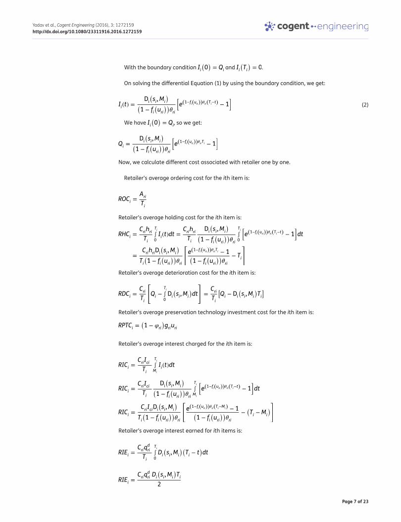
Now, we calculate different cost associated with retailer one by one.
Retailer’s average ordering cost for the ith item is:
Retailer’s average holding cost for the ith item is:
Retailer’s average deterioration cost for the ith item is:
Retailer’s average preservation technology investment cost for the ith item is:
Retailer’s average interest charged for the ith item is:
Retailer’s average interest earned for ith items is:
(2)Ii(t) =Di(si ,Mi
)(1 − fi
(uri
))�ri
[e(1−fi(uri))�ri(Ti−t) − 1
]
Qi =Di(si ,Mi
)(1 − fi
(uri
))�ri
[e(1−fi(uri))�ri Ti − 1
]
ROCi =AriTi
RHCi =CrihriTi
Ti
∫0
Ii(t)dt =CrihriTi
Di
(si ,Mi
)(1 − fi
(uri
))�ri
Ti
∫0
[e(1−fi(uri))�ri(Ti−t) − 1
]dt
=CrihriDi
(si ,Mi
)
Ti(1 − fi
(uri
))�ri
[e(1−fi(uri))�ri Ti − 1(1 − fi
(uri
))�ri
− Ti
]
RDCi =CriTi
[Qi −
Ti
∫0
Di(si ,Mi
)dt
]=CriTi
[Qi − Di
(si ,Mi
)Ti]
RPTCi =(1 − �ri
)griuri
RICi =CriIciTi
Ti
∫Mi
Ii(t)dt
RICi =CriIciTi
Di(si ,Mi
)(1 − fi
(uri
))�ri
Ti
∫Mi
[e(1−fi(uri))�ri(Ti−t) − 1
]dt
RICi =CriIciDi
(si ,Mi
)
Ti(1 − fi
(uri
))�ri
[e(1−fi(uri))�ri(Ti−Mi) − 1(
1 − fi(uri
))�ri
−(Ti −Mi
)]
RIEi =Criq
dri
Ti
Ti
∫0
Di(si ,Mi
)(Ti − t
)dt
RIEi =Criq
dri Di
(si ,Mi
)Ti
2
Page 8 of 23
Yadav et al., Cogent Engineering (2016), 3: 1272159http://dx.doi.org/10.1080/23311916.2016.1272159
Therefore, the retailer’s total average cost for the ith item is:
Hence, the retailer’s total average cost is given by:
3.2. Formulation of manufacturer mathematical modelThe manufacturer starts manufacturing process from time t = 0 and whole of its inventory vanish at time t = niTi for the ith item. It is the time when the retailer receives last replenishment of the ith item. The manufacturing process of ith item continues up to that period of time so that total demand of ith item of retailer i.e. niQi can be satisfied. Inventory level of manufacturer increase that period of time and after that every cycle of time Ti, the inventory level of manufacturer decreases by the amount Qi due to the demand of retailer for the ith item as shown in Figure 1.
Manufacturer’s average holding cost for the ith item is:
Manufacturer’s average setup cost for ith item is:
Manufacturer’s average manufacturing cost for the ith item is:
Manufacturer’s average opportunity interest loss for the ith item is:
Manufacturer’s average transportation cost for the ith item is:
Therefore, the manufacturer’s total average cost for the ith item is:
TRi(Mi , Ti
)= ROCi + RHCi + RDCi + RPTCi + RICi − RIEi
(3)
TR(Mi , Ti
)=
n∑i=1
TRi(Mi , Ti
)=
n∑i=1
[ROCi + RHCi + RDCi + RPTCi + RICi − RIEi
]
=
n∑i=1
[AriTi
+CrihriDi
(si ,Mi
)
Ti(1 − fi
(uri
))�ri
[e(1−fi(uri))�ri Ti − 1(1 − fi
(uri
))�ri
− Ti
]+CriTi
[Qi − Di
(si ,Mi
)Ti]
+(1 − �ri
)griuri +
CriIciDi(si ,Mi
)
Ti(1 − fi
(uri
))�ri
[e(1−fi(uri))�ri(Ti−Mi) − 1(
1 − fi(uri
))�ri
−(Ti −Mi
)]−Criq
dri Di
(si ,Mi
)Ti
2
]
MHCi =hminiTi
[niQi −
1
2niQi
niQiPmi
− Qi{Ti + 2Ti + 3Ti +…+ (ni − 1)Ti
}]=hmiQi2
[(ni + 1) −
niQiTiPmi
]
MSCi =SminiTi
MMCi =M(Pmi
)Qi
Ti
MOILi =qdmiCriMiQi
Ti
MTCi =TCmiTi
Page 9 of 23
Yadav et al., Cogent Engineering (2016), 3: 1272159http://dx.doi.org/10.1080/23311916.2016.1272159
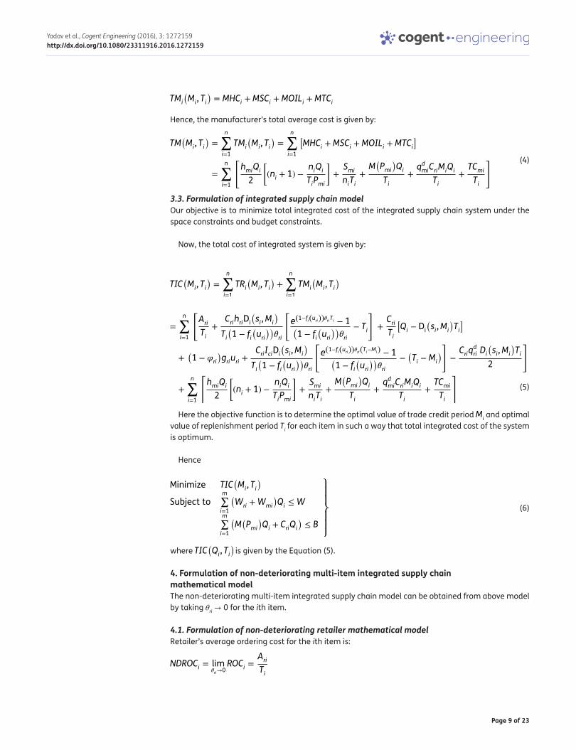
Hence, the manufacturer’s total average cost is given by:
3.3. Formulation of integrated supply chain modelOur objective is to minimize total integrated cost of the integrated supply chain system under the space constraints and budget constraints.
Now, the total cost of integrated system is given by:
Here the objective function is to determine the optimal value of trade credit period Mi and optimal value of replenishment period Ti for each item in such a way that total integrated cost of the system is optimum.
Hence
where TIC(Qi , Ti
) is given by the Equation (5).
4. Formulation of non-deteriorating multi-item integrated supply chain mathematical modelThe non-deteriorating multi-item integrated supply chain model can be obtained from above model by taking θri → 0 for the ith item.
4.1. Formulation of non-deteriorating retailer mathematical modelRetailer’s average ordering cost for the ith item is:
TMi
(Mi , Ti
)= MHCi +MSCi +MOILi +MTCi
(4)
TM(Mi , Ti
)=
n∑i=1
TMi
(Mi , Ti
)=
n∑i=1
[MHCi +MSCi +MOILi +MTCi
]
=
n∑i=1
[hmiQi2
[(ni + 1) −
niQiTiPmi
]+SminiTi
+M(Pmi
)Qi
Ti+qdmiCriMiQi
Ti+TCmiTi
]
TIC(Mi , Ti
)=
n∑i=1
TRi(Mi , Ti
)+
n∑i=1
TMi
(Mi , Ti
)
(5)
=
n∑i=1
[AriTi
+CrihriDi
(si ,Mi
)
Ti(1 − fi
(uri
))�ri
[e(1−fi(uri))�ri Ti − 1(1 − fi
(uri
))�ri
− Ti
]+CriTi
[Qi − Di
(si ,Mi
)Ti]
+(1 − �ri
)griuri +
CriIciDi(si ,Mi
)
Ti(1 − fi
(uri
))�ri
[e(1−fi(uri))�ri(Ti−Mi) − 1(
1 − fi(uri
))�ri
−(Ti −Mi
)]−Criq
dri Di
(si ,Mi
)Ti
2
]
+
n∑i=1
[hmiQi2
[(ni + 1) −
niQiTiPmi
]+SminiTi
+M(Pmi
)Qi
Ti+qdmiCriMiQi
Ti+TCmiTi
]
(6)
Minimize TIC�Mi , Ti
�
Subject tom∑i=1
�Wri +Wmi
�Qi ≤W
m∑i=1
�M�Pmi
�Qi + CriQi
�≤ B
⎫⎪⎪⎬⎪⎪⎭
NDROCi = lim�ri→0
ROCi =AriTi
Page 10 of 23
Yadav et al., Cogent Engineering (2016), 3: 1272159http://dx.doi.org/10.1080/23311916.2016.1272159
Retailer’s average holding cost for the ith item is:
Retailer’s average deterioration cost for the ith item is:
Retailer’s average preservation technology investment cost for the ith item is:
NDRPTCi = lim�ri→0
RPTCi = 0 (as there is no deterioration so there is no need to invest in preserva-
tion technology).
Retailer’s average interest charged for the ith item is:
Retailer’s average interest earned for ith items is:
Therefore, the retailer’s total average cost for the ith item is:
Hence, the retailer’s total average cost is given by:
4.2. Formulation of non-deteriorating manufacturer mathematical modelManufacturer’s average holding cost for the ith item is:
Manufacturer’s average setup cost for ith item is:
Yadav et al., Cogent Engineering (2016), 3: 1272159http://dx.doi.org/10.1080/23311916.2016.1272159
Manufacturer’s average manufacturing cost for the ith item is:
Manufacturer’s average opportunity interest loss for the ith item is:
Manufacturer’s average transportation cost for the ith item is:
Therefore, the manufacturer’s total average cost for the ith item is:
Hence, the manufacturer’s total average cost is given by:
4.3. Formulation of non-deteriorated integrated supply chain modelOur objective is to minimize total integrated cost of non-deteriorating integrated supply chain sys-tem under the space constraints and budget constraints.
Now, the total cost of integrated system is given by:
Here the objective function is to determine the optimal value of trade credit period Mi and optimal value of replenishment period Ti for each item in such a way that total integrated cost of the system for non-deteriorated items is optimum.
Hence
where NDTIC(Mi , Ti
) is given by the Equation (9).
NDMMCi = lim�ri→0
MMCi = lim�ri
M(Pmi
)Qi
Ti= M
(Pmi
)Di
NDMOILi = lim�ri→0
MOILi = lim�ri
qdmiCriMiQiTi
= qdmiCriMiDi
NDMTCi = lim�ri→0
MTCi = lim�ri→0
TCmiTi
=TCmiTi
NDTMi
(Mi , Ti
)= NDMHCi + NDMSCi + NDMOILi + NDMTCi
(8)
NDTM(Mi , Ti
)=
n∑i=1
NDTMi
(Mi , Ti
)=
n∑i=1
[NDMHCi + NDMSCi + NDMOILi + NDMTCi
]
=
n∑i=1
[hmiDiTi2
[(ni + 1) −
niDiPmi
]+SminiTi
+M(Pmi
)Di + q
dmiCriMiDi +
TCmiTi
]
(9)NDTIC
(Mi , Ti
)=
n∑i=1
NDTRi(Mi , Ti
)+
n∑i=1
NDTMi
(Mi , Ti
)
=
n∑i=1
[AriTi
+CrihriDi
(si ,Mi
)Ti
2+CriIciDi
(si ,Mi
)(Ti −Mi
)22Ti
−Criq
dri Di
(si ,Mi
)Ti
2
+hmiDiTi2
[(ni + 1) −
niDiPmi
]+SminiTi
+M(Pmi
)Di + q
dmiCriMiDi +
TCmiTi
]
(10)
Minimize NDTIC�Mi , Ti
�
Subject tom∑i=1
�Wri +Wmi
�Qi ≤W
m∑i=1
�M�Pmi
�Qi + CriQi
�≤ B
⎫⎪⎪⎬⎪⎪⎭
Page 12 of 23
Yadav et al., Cogent Engineering (2016), 3: 1272159http://dx.doi.org/10.1080/23311916.2016.1272159
5. Solution procedureFrom Equation (6) it is observed that the objective function is non-linear. So it is a non-linear problem model which cannot be solved easily by the exact method. Hence, a simple Lagrangian multiplier (similar to Uthayakumar and Priyan, (2013)) is used to solve the problem.
In the present problem, there are two constraints imposed simultaneously in inventory system. To solve such type of problem, we can follow the following steps:
Step 1: First we obtain the optimal value (M∗
i , T∗
i
) of decision variables by ignoring space con-
straints and budget constraints.
Objective function is
Objective function TIC(Mi , Ti
) is a function of 2n variables M1, M2, …, Mn, T1, T2, ..., Tn.
Necessary conditions: A necessary conditions for the minimum of TIC(Mi , Ti
) (where i = 1, 2, ..., n)
give
TIC(Mi , Ti
)
=
n∑i=1
[AriTi
+CrihriDi
(si ,Mi
)
Ti(1 − fi
(uri
))�ri
[e(1−fi(uri))�ri Ti − 1(1 − fi
(uri
))�ri
∨̀⃛(Ti∨̀⃛Mi)
]+CriTi
[Qi − Di
(si ,Mi
)Ti]
+(1 − �ri
)griuri +
CriIciDi(si ,Mi
)
Ti(1 − fi
(uri
))�ri
[e(1−fi(uri))�ri(Ti−Mi) − 1(
1 − fi(uri
))�ri
−(Ti −Mi
)]−Criq
dri Di
(si ,Mi
)Ti
2
]
+
n∑i=1
[hmiQi2
[(ni + 1) −
niQiTiPmi
]+SminiTi
+M(Pmi
)Qi
Ti+qdmiCriMiQi
Ti+TCmiTi
]
(11)
�TIC(Mi , Ti
)�Ti
= 0,�TIC
(Mi , Ti
)�Mi
= 0 −Ari
T2i−
CrihriDi(si ,Mi
)
T2i(1 − fi
(uri
))�ri
[e(1−fi(uri))�ri Ti − 1(1 − fi
(uri
))�ri
− Ti
]
+CrihriDi
(si ,Mi
)
Ti(1 − fi
(uri
))�ri
[e(1−fi(uri))�ri Ti − 1
]−Cri
T2i
[Qi − Di
(si ,Mi
)Ti]+CriTi
[Di
(si ,Mi
)e(1−fi(uri))�ri Ti − D
i
(si ,Mi
)]
−CriIciDi
(si ,Mi
)
T2i(1 − fi
(uri
))�ri
[e(1−fi(uri))�ri(Ti−Mi) − 1(
1 − fi(uri
))�ri
−(Ti −Mi
)]
+CriIciDi
(si ,Mi
)
Ti(1 − fi
(uri
))�ri
[e(1−fi(uri))�ri(Ti−Mi) − 1
]−Criq
dri Di
(si ,Mi
)2
+hmiDi
(si ,Mi
)e(1−fi(uri))�ri Ti
2
[(ni + 1) −
niQiTiPmi
]
+hmiQi2
[niQi
T2i Pmi−niDi
(si ,Mi
)e(1−fi(uri))�ri Ti
TiPmi
]−1
T2i
[Smini
+M(Pmi
)Qi + q
dmiQi + q
dmiCriMiQi + TCmi
]
+Di
(si ,Mi
)e(1−fi(uri))�ri Ti
Ti
[M(Pmi
)+ qdmi + q
dmiCriMi
]= 0
Page 13 of 23
Yadav et al., Cogent Engineering (2016), 3: 1272159http://dx.doi.org/10.1080/23311916.2016.1272159
On solving Equations (11) and (12) simultaneously we get the value of Mi and Ti.
Sufficient condition: A sufficient condition for TIC(Mi , Ti
) to have a relative minimum at
(M∗
i , T∗
i
)
is that the following Hessian matrix is positive definite.
If optimal value (M∗
i , T∗
i
) satisfies both the constraints, then obtained values of decision variables
are optimal solutions such that the integrated total cost is minimum and go to step 5.
Step2: Else solve the optimization problem subject to space constraint and ignore the budget constraint. The Lagrange function, L, can be defined as follows by introducing one Lagrangian mul-tiplier � to the space constraint.
Lagrangian function L(Mi , Ti , �
) is a function of 2n + 1 variables M1, M2, ..., Mn, T1, T2, ..., Tn, �.
(12)
hriTi(1 − fi(uri))�ri
�e(1−fi (uri ))�riTi − 1
(1 − fi(uri))�ri− Ti
��C1rie
MiDi�si ,Mi
�+ Cri
�−�ri
�sri��1 − ri
�Mi log�1 − ri
�
+ �ri
�sri��1 − ri
�Mi log�1 − ri
���+C1rie
Mi
Ti
�Qi − Di
�si ,Mi
�Ti�
+CriTi
�Qi −
�−�ri
�sri��1 − ri
�Mi log�1 − ri
�+ �ri
�sri��1 − ri
�Mi log�1 − ri
��Ti
�
+
⎡⎢⎢⎢⎣
C1rieMi IciDi
�si ,Mi
�Ti(1 − fi(uri))�ri
+
CriIci
�−�ri
�sri��1 − ri
�Mi log�1 − ri
�+ �ri
�sri��1 − ri
�Mi log�1 − ri
��
Ti(1 − fi(uri))�ri
⎤⎥⎥⎥⎦
×
�e(1−fi (uri ))�ri(Ti−Mi) − 1
(1 − fi(uri))�ri−�Ti −Mi
��+CriIciDi
�si ,Mi
�Ti(1 − fi(uri))�ri
�1 − e(1−fi (uri ))�ri(Ti−Mi)
�
−C1rie
Miqdri Di�si ,Mi
�Ti
2−
Criqdri
�−�ri
�sri��1 − ri
�Mi log�1 − ri
�+ �ri
�sri��1 − ri
�Mi log�1 − ri
��Ti
2
⎤⎥⎥⎥⎦
+qdmiQiTi
�Cri +MiC
1rie
Mi
�= 0
⎡⎢⎢⎢⎢⎢⎢⎢⎢⎢⎢⎢⎢⎢⎣
TICM1M1TICM1M2
… TICM1MnTICM1T1
TICM1T2… TICM1Tn
TICM2M1TICM2M2
… TICM2MnTICM2T1
TICM2T2… TICM2Tn
… … … … … … … …
… … … … … … … …
TICMnM1TICMnM2
… TICMnMnTICMnT1
TICMnT2… TICMnTn
TICT1M1TICT1M2
… TICT1MnTICT1T1
TICT1T2… TICT1Tn
TICT2M1TICT2M2
… TICT2MnTICT2T1
TICT2T2… TICT2Tn
… … … … … … … …
… … … … … … … …
TICTnM1TICTnM2
… TICTnMnTICTnT1
TICTnT2… TICTnTn
⎤⎥⎥⎥⎥⎥⎥⎥⎥⎥⎥⎥⎥⎥⎦
L(Mi , Ti , �
)= TIC
(Mi , Ti
)+ �
[W −
m∑i=1
(Wri +Wmi
)Qi
]
Page 14 of 23
Yadav et al., Cogent Engineering (2016), 3: 1272159http://dx.doi.org/10.1080/23311916.2016.1272159
Necessary conditions: A necessary conditions for the minimum of L(Mi , Ti , �
) (where i = 1, 2, ..., n)
give:
On solving Equations (13)–(15) simultaneously we get the value of Mi, Ti and �.
Sufficient condition: A sufficient condition for TIC(Mi , Ti
) to have a relative minimum at
(M∗
i , T∗
i
)
is that the following bordered Hessian matrix is positive definite.
�L(Mi , Ti , �
)�Mi
= 0,�L
(Mi , Ti , �
)�Mi
= 0,�L
(Mi , Ti , �
)��
= 0
(13)
−Ari
T2i−
CrihriDi(si ,Mi
)
T2i(1 − fi
(uri
))�ri
[e(1−fi(uri))�ri Ti − 1(1 − fi
(uri
))�ri
− Ti
]+
CrihriDi(si ,Mi
)
Ti(1 − fi
(uri
))�ri
[e(1−fi(uri))�ri Ti − 1
]
−Cri
T2i
[Qi − Di
(si ,Mi
)Ti]+CriTi
[Di
(si ,Mi
)e(1−fi(uri))�ri Ti − D
i
(si ,Mi
)]−
CriIciDi(si ,Mi
)
T2i(1 − fi
(uri
))�ri
×
[e(1−fi(uri))�ri(Ti−Mi) − 1(
1 − fi(uri
))�ri
−(Ti −Mi
)]+
CriIciDi(si ,Mi
)
Ti(1 − fi
(uri
))�ri
[e(1−fi(uri))�ri(Ti−Mi) − 1
]
−Criq
dri Di
(si ,Mi
)2
+hmiDi
(si ,Mi
)e(1−fi(uri))�ri Ti
2
[(ni + 1) −
niQiTiPmi
]
+hmiQi2
[niQi
T2i Pmi−niDi
(si ,Mi
)e(1−fi(uri))�ri Ti
TiPmi
]−1
T2i
[Smini
+M(Pmi
)Qi + q
dmiQi + q
dmiCriMiQi + TCmi
]
+Di
(si ,Mi
)e(1−fi(uri))�ri Ti
Ti
[M(Pmi
)+ qdmi + q
dmiCriMi
]− �
m∑i=1
(Wri +Wmi
)Di
(si ,Mi
)e(1−fi(uri))�ri Ti = 0
(14)
hri
Ti�1 − fi
�uri
���ri
�e(1−fi(uri))�ri Ti − 1�1 − fi
�uri
���ri
− Ti
��C1rie
MiDi�si ,Mi
�+ Cri
�−�ri
�sri��1 − ri
�Mi log�1 − ri
�
+ �ri
�sri��1 − ri
�Mi log�1 − ri
���+C1rie
Mi
Ti
�Qi − Di
�si ,Mi
�Ti�
+CriTi
�Qi −
�−�ri
�sri��1 − ri
�Mi log�1 − ri
�+ �ri
�sri��1 − ri
�Mi log�1 − ri
��Ti
�
+
⎡⎢⎢⎢⎣
C1rieMi IciDi
�si ,Mi
�Ti(1 − fi(uri))�ri
+
CriIci
�−�ri
�sri��1 − ri
�Mi log�1 − ri
�+ �ri
�sri��1 − ri
�Mi log�1 − ri
��
Ti(1 − fi(uri))�ri
⎤⎥⎥⎥⎦
×
�e(1−fi (uri ))�ri(Ti−Mi) − 1
(1 − fi(uri))�ri−�Ti −Mi
��+CriIciDi
�si ,Mi
�Ti(1 − fi(uri))�ri
�1 − e(1−fi (uri ))�ri(Ti−Mi)
�
−C1rie
Miqdri Di�si ,Mi
�Ti
2−
Criqdri
�−�ri
�sri��1 − ri
�Mi log�1 − ri
�+ �ri
�sri��1 − ri
�Mi log�1 − ri
��Ti
2
⎤⎥⎥⎥⎦
+qdmiQiTi
�Cri +MiC
1rie
Mi
�= 0
(15)
[W −
m∑i=1
(Wri +Wmi
)Qi
]= 0
Page 15 of 23
Yadav et al., Cogent Engineering (2016), 3: 1272159http://dx.doi.org/10.1080/23311916.2016.1272159
If optimal value (M∗
i , T∗
i
) satisfies budget constraints, then obtained values of decision variables are
optimal solutions such that the integrated total cost is minimum and go to step 5.
Step 3: Else solve the optimization problem subject to budget constraint and ignore the space constraint. The Lagrange function, L, can be defined as follows by introducing one Lagrangian mul-tiplier � to the space constraint.
Lagrangian function L(Mi , Ti ,�
) is a function of 2n+1 variables M1, M2, ..., Mn, T1, T2, ..., Tn, �.
In this step whole of the computational process is same as step-2.
If optimal value (M∗
i , T∗
i
) satisfies space constraints, then obtained values of decision variables are
optimal solutions such that the integrated total cost is minimum and go to step 5.
Step 4: If none of the above three step is applicable, solve the optimization problem subject to both space constraint and the budget constraint. The Lagrange function, L, can be defined as follows by introducing one Lagrangian multiplier � to the space constraint.
Lagrangian function L(Mi , Ti , �
) is a function of 2n+2 variables M1, M2, ..., Mn, T1, T2, ..., Tn, �,�.
Necessary conditions: The necessary conditions for the minimum of L(Mi , Ti , �,�
) (where i = 1, 2,
..., n) give:
⎡⎢⎢⎢⎢⎢⎢⎢⎢⎢⎢⎢⎢⎢⎢⎢⎣
TICM1M1TICM1M2
… TICM1MnTICM1T1
TICM1T2… TICM1Tn
gM1
TICM2M1TICM2M2
… TICM2MnTICM2T1
TICM2T2… TICM2Tn
gM2
… … … … … … … … …
… … … … … … … … …
TICMnM1TICMnM2
… TICMnMnTICMnT1
TICMnT2… TICMnTn
gMn
TICT1M1TICT1M2
… TICT1MnTICT1T1
TICT1T2… TICT1Tn
gT1TICT2M1
TICT2M2… TICT2Mn
TICT2T1TICT2T2
… TICT2TngT2
… … … … … … … … …
… … … … … … … … …
TICTnM1TICTnM2
… TICTnMnTICTnT1
TICTnT2… TICTnTn
gTngM1
gM2… gMn
gT1gT2
… gTn0
⎤⎥⎥⎥⎥⎥⎥⎥⎥⎥⎥⎥⎥⎥⎥⎥⎦
L(Mi , Ti ,�
)= TIC
(Mi , Ti
)+ �
[B −
m∑i=1
(M(Pmi
)Qi + CriQi
)]
L(Mi , Ti , �,�
)= TIC
(Mi , Ti
)+ �
[W −
m∑i=1
(Wri +Wmi
)Qi
]+ �
[B −
m∑i=1
(M(Pmi
)Qi + CriQi
)]
Page 16 of 23
Yadav et al., Cogent Engineering (2016), 3: 1272159http://dx.doi.org/10.1080/23311916.2016.1272159
On solving Equations (16)–(19) simultaneously we get the value of Mi, Ti and �,�.
Yadav et al., Cogent Engineering (2016), 3: 1272159http://dx.doi.org/10.1080/23311916.2016.1272159
Sufficient condition: A sufficient condition for TIC(Mi , Ti
) to have a relative minimum at
(M∗
i , T∗
i
)
is that the following bordered Hessian matrix is positive definite.
Values of (M∗
i , T∗
i
) are such that the objective function integrated system is optimum and satisfies
both the constraints and go to step 5.
Step 5: Stop.
6. Numerical analysisThe purposes of numerical analysis are as follows:
(1) Obtain the optimal solution to illustrate the developed model.
(2) Through sensitive analysis, we try to highlights how the different parameters effect the opti-mal solution.
6.1. Numerical exampleIn order to illustrate the developed model, let us consider the following study.
XYZ is a telecommunication firm in India which was established in 2010. It is a joint venture of two companies named as X and Y to manufacture smartphones. XYZ Mobiles India pvt Ltd. has a strategic tie-up between X and Y. The role of company X (which is known as manufacturer) is to manufacturer three different smartphones (S1, S2, S3) of different range whereas company Y (which is known as retailer) deals the marketing and sales department.
Manufacturing rate of S1, S1, S3 are respectively 1,500, 1,300, 1,250 units per year. Different com-ponent of unit manufacturing cost of phones are described in Tables 1 and 2.
Different component of transportation cost from manufacturer to retailer are described in Table 3.
From survey it is observed that different cost component regarding retailer are described in Table 4.
Deterioration occurs at the end of retailer. So retailer uses preservation technology to reduce the rate of deterioration as much as possible. Different cost component and other parameters are de-scribed in Table 5.
Here, fi(uri
)= 1 − e−�uri where γ = 0.5
⎡⎢⎢⎢⎢⎢⎢⎢⎢⎢⎢⎢⎢⎢⎢⎢⎢⎣
TICM1M1TICM1M2
… TICM1MnTICM1T1
TICM1T2… TICM1Tn
gM1fM1
TICM2M1TICM2M2
… TICM2MnTICM2T1
TICM2T2… TICM2Tn
gM2fM2
… … … … … … … … … …
… … … … … … … … … …
TICMnM1TICMnM2
… TICMnMnTICMnT1
TICMnT2… TICMnTn
gMnfMn
TICT1M1TICT1M2
… TICT1MnTICT1T1
TICT1T2… TICT1Tn
gT1fT1
TICT2M1TICT2M2
… TICT2MnTICT2T1
TICT2T2… TICT2Tn
gT2fT2
… … … … … … … … … …
… … … … … … … … … …
TICTnM1TICTnM2
… TICTnMnTICTnT1
TICTnT2… TICTnTn
gTnfTn
gM1gM2
… gMngT1
gT2… gTn
0 0
fM1fM2
… fMnfT1
fT2… fTn
0 0
⎤⎥⎥⎥⎥⎥⎥⎥⎥⎥⎥⎥⎥⎥⎥⎥⎥⎦
Page 18 of 23
Yadav et al., Cogent Engineering (2016), 3: 1272159http://dx.doi.org/10.1080/23311916.2016.1272159
To strengthen the integrated system, manufacturer provides the trade credit period to the retailer. Regarding this values of the parameters are described in Table 6.
Space constraints and budget constraints are imposed to obtain solution of optimal solution. Total space available to store items is 6,000 sq. ft. and $98,000 is available to invest in business. Regarding this values of the parameters are described in Table 7.
Here it is assumed that demand of customer at the end retailer depends on selling price and trade credit offered by manufacturer to the retailer (see Table 8).
Now, problem is to determine optimal value of trade credit period offered by manufacturer and replenishment period, so the total integrated inventory cost of the supply chain is minimum.
Using the solution procedure discussed in Section 3.5, we can get the optimal values of decision variables and objective function (see Table 9).
Table 5. Parameters related to preservation technology cost and rate of deteriorationFor S1 For S2 For S3θr1 ur1 φr1 gr1 θr2 ur2 φr2 gr2 θr3 ur3 φr3 gr3
0.05 10 0.02 8 0.10 13 0.03 7 0.15 12 0.02 9
Table 4. Retailer’s ordering cost, procurement cost, holding cost, and selling priceFor S1 For S2 For S3Ar1 C
Table 3. Different parameters of transportation costFor S1 For S2 For S3
TC0
m1TC
1
m1TC
0
m2TC
1
m2TC
0
m3TC
1
m3
150 0.04 160 0.02 155 0.03
Table 2. Holding cost and setup cost for manufacturerFor S1 For S2 For S3Holding cost ($)
Setup cost ($) Holding cost ($)
Setup cost ($) Holding cost ($)
Setup cost ($)
hm1 Sm1 hm2 Sm2 hm3 Sm3
6 3,000 5 3,500 7 3,300
Table 1. Different parameters of unit manufacturing costFor S1 For S2 For S3Mm1 Gm1 Bm1 γ1 Mm1 Gm1 Bm2 γ2 Mm3 Gm3 Bm3 γ3
15 60 5 0.0006 18 70 3 0.0005 20 55 4 0.0007
Page 19 of 23
Yadav et al., Cogent Engineering (2016), 3: 1272159http://dx.doi.org/10.1080/23311916.2016.1272159
6.2. Sensitivity analysisIn this section, the sensitivity analysis on the equilibrium strategies with respect to different key parameters is carried out. This analysis is carried out by changing one parameter and remaining the others fixed.
6.2.1. Sensitivity w.r.t holding costFrom Figure 2 it is observed that as the holding cost of the retailer and manufacturer increases the total inventory cost of retailer, manufacturer and integrated system also increases. But change is cost higher in case of retailer whereas it is least in case of manufacturer. As the holding cost in-creases from −50 to + 50%, the ordering quantity decreases as a result total inventory cost of inte-grated system increases.
6.2.2. Sensitivity w.r.t selling priceFigure 3 shows that as the selling price increases total inventory cost of retailer, manufacturer and integrated system decreases. This is due to as selling price increases demand of items decreases therefore ordering quantity decreases and hence total inventory cost decreases.
6.2.3. Sensitivity w.r.t trade credit periodFigure 4 shows the effect of trade credit period on the optimal solution. It is observed that as the trade credit period increases retailer’s, manufacturer’s and integrated inventory cost is also increas-es. As trade credit period increases, demand increases, ordering quantity increases therefore hold-ing cost increases and hence total inventory cost of the integrated system increases.
Table 9. Optimum resultsItem ni Mi Ti cri Qi TR TM TIC1 6 0.0628 0.15253 25.851 96.519 5,605.016 112,065.246 117,670.262
2 6 0.0598 0.15253 35.743 90.490
3 6 0.0601 0.15253 40.955 99.966
Table 8. Parameters related to demandFor S1 For S2 For S3r1 αr1(sr1) βr1(sr1) r2 αr2(sr2) βr2(sr2) r3 αr2(sr2) βr3(sr3)0.35 5,000–
1.21sr1
600–1.21sr1
0.37 4,800–1.21sr2
550–1.21sr2
0.36 5,200–1.21sr3
600–1.21sr3
Table 7. Parameters related to space constraintsFor S1 For S2 For S3Wr1 Wm1 Wr2 Wm2 Wr3 Wm3
5 15 6 16 7 17
Table 6. Different parameters related to trade creditFor S1 For S2 For S3Ici q
d
riqd
miIci q
d
riqd
miIci q
d
riqd
mi
0.07 0.05 0.04 0.06 0.03 0.04 0.05 0.03 0.03
Page 20 of 23
Yadav et al., Cogent Engineering (2016), 3: 1272159http://dx.doi.org/10.1080/23311916.2016.1272159
6.2.4. Sensitivity w.r.t procurement costFigure 5 reflects the effect of procurement cost on the inventory cost of retailer, manufacturer and integrated system. As procurement cost increases the holding cost increases and interest charged by the manufacturer increases and hence total inventory cost of retailer, manufacturer and inte-grated system increases. Retailer’s inventory cost is highly affected by the procurement cost but its effect is least in case of manufacturer.
Figure 4. Effect of trade credit period on inventory cost.
-15
-10
-5
0
5
10
15
-50 -25 25 50
% C
hang
e in
Inv
ento
ry C
ost
% Change in Trade Credit Period
Retailer's Cost
Manufacturer's Cost
Integrated Cost
Figure 3. Effect of selling price on inventory cost.
-3
-2
-1
0
1
2
3
-50 -25 25 50
% C
hang
e in
Inv
ento
ry C
ost
% Change in Selling Price
Retailer's Cost
Manufacturer' Cost
Integrated Cost
Figure 2. Effect of holding cost on inventory cost.
-30
-20
-10
0
10
20
30
-50 -25 25 50%
Cha
nge
in I
nven
tory
Cos
t
% Change in Holding Cost
Retailer's Cost
Manufacturer' Cost
Integrated Cost
Page 21 of 23
Yadav et al., Cogent Engineering (2016), 3: 1272159http://dx.doi.org/10.1080/23311916.2016.1272159
7. ConclusionIn this paper, a more practical multi-item integrated inventory system involving one manufacturer and one retailer is introduced. Two models are developed here one with deterioration and the other without deterioration. Multivariable demand is considered here which increases due to increase in trade credit period and decreases due to increase in selling price. Whole of the analysis is carried out over finite planning horizon. Addition cost to use the preservation technology in order to maintain the worth of items as long as possible is considered here. Long term bonding between manufacturer and retailer is developed by offering trade credit period to the retailer by the manufacturer. Cost minimization methodology is used here to find the optimal solution of the proposed model. Lagarangian Multiplier Method (LMM) is used to obtain the optimal value of objective function sub-ject to space constraints and budget constraints. Validity of proposed model is illustrated with the help of numerical example. Managerial outcomes of numerical results are obvious and provide a suitable framework to reduce the integrated cost of the supply chain. Sensitive analysis is carried out with respect to holding cost, procurement cost, selling price and trade credit. Inventory cost of re-tailer is highly affected by procurement cost and holding cost. The proposed model incorporates practical features that are likely to relate with some kinds of inventory. Some of the advantages of the proposed model are as follows:
(1) There is hardly any supply chain which focused on only single item. So considering multi-item problem is more practical approach.
(2) Consideration of budget constraint and space constrain make the model realistic as ignorance of these restriction results in infeasible solution.
(3) Making provision of some budget for preservation technology increase the goodwill of the firm in the market.
(4) Providing trade credit strengthens the supply chain coordination.
This analysis will help the inventory practitioners of seasonal products such as fashionable goods, warm cloths, domestic goods and medicines. There are several ideas to extend the present model to make it more practical. In this study we have considered constant rate of deterioration. But in future, it may be taken as time dependent. Shortages may also be considered to make it more useful. This analysis can be carried out under effect of inflation in future.
Figure 5. Effect of procurement cost on inventory cost.
-25-20-15-10-505
10152025
-50 -25 25 50
% C
hang
e in
Inv
ento
ry C
ost
% Change in Procurement Cost
Retailer's Cost
Manufactrer' Cost
Integrated Cost
Page 22 of 23
Yadav et al., Cogent Engineering (2016), 3: 1272159http://dx.doi.org/10.1080/23311916.2016.1272159
FundingThe authors received no direct funding for this research.
E-mail: [email protected] Department of Mathematics, Vardhaman (P.G.) College,
Bijnor 246701, Uttar Pradesh, India.2 Department of Mathematics, C.C.S. University, Meerut
250001, Uttar Pradesh, India.3 Department of Mathematics, Banasthali University,
Banasthali 304022, Rajasthan, India.
Citation informationCite this article as: Multi-item multi-constraint supply chain integrated inventory model with multi-variable demand under the effect of preservation technology, Dharmendra Yadav, S.R. Singh & Vandana Arora, Cogent Engineering (2016), 3: 1272159.
ReferencesCárdenas-Barrón, L. E., & Sana, S. S. (2014). A production-
inventory model for a two-echelon supply chain when demand is dependent on sales teams׳ initiatives. International Journal of Production Economics, 155, 249–258. http://dx.doi.org/10.1016/j.ijpe.2014.03.007
Chakraborty, D., Jana, D. K., & Roy, T. P. (2015). Multi-item integrated supply chain model for deteriorating items with stock dependent demand under fuzzy random and bifuzzy environments. Computers & Industrial Engineering, 88, 166–180. http://dx.doi.org/10.1016/j.cie.2015.06.022
Das, D., Kar, M. B., Roy, A., & Kar, S. (2012). Two-warehouse production model for deteriorating inventory items with stock-dependent demand under inflation over a random planning horizon. Central European Journal of Operations Research, 20, 251–280. http://dx.doi.org/10.1007/s10100-010-0165-4
Das, K., Roy, T. K., & Maiti, M. (2000). Multi-item inventory model with quantity-dependent inventory costs and demand-dependent unit cost under imprecise objective and restrictions: A geometric programming approach. Production Planning & Control, 11, 781–788. http://dx.doi.org/10.1080/095372800750038382
Das, K., Roy, T. K., & Maiti, M. (2004). Multi-item stochastic and fuzzy-stochastic inventory models under two restrictions. Computers & Operations Research, 31, 1793–1806. http://dx.doi.org/10.1016/S0305-0548(03)00120-5
Dye, C. Y., Ouyang, L. Y., & Hsieh, T. P. (2007). Inventory and pricing strategies for deteriorating items with shortages: A discounted cash flow approach. Computers & Industrial Engineering, 52, 29–40. http://dx.doi.org/10.1016/j.cie.2006.10.009
Guchhait, P., Maiti, M. K., & Maiti, M. (2010). Multi-item inventory model of breakable items with stock-dependent demand under stock and time-dependent breakability rate. Computers and Industrial Engineering, 59, 911–920. http://dx.doi.org/10.1016/j.cie.2010.09.001
Jaber, M. Y., & Osman, I. H. (2006). Coordinating a two-level supply chain with delay in payments and profit sharing. Computers & Industrial Engineering, 50, 385–400. http://dx.doi.org/10.1016/j.cie.2005.08.004
Jana, D. K., Das, B., & Maiti, M. (2014). Multi-item partial backlogging inventory models over random planninghorizon in random fuzzy environment. Applied
Kin Chan, C., Lee, Y. C. E., & Goyal, S. K. (2010). A delayed payment method in co-ordinating a single-vendor multi-buyer supply chain. International Journal of Production Economics, 127, 95–102. http://dx.doi.org/10.1016/j.ijpe.2010.04.046
Lin, C., Tan, B., & Lee, W. C. (2000). An EOQ model for deteriorating items with time varying demand and shortages. International Journal of Systems Science, 31, 391–400. http://dx.doi.org/10.1080/002077200291235
Maity, K., & Maiti, M. (2007). Possibility and necessity constraints and their defuzzification—A multi-item production-inventory scenario via optimal control theory. European Journal of Operational Research, 177, 882–896. http://dx.doi.org/10.1016/j.ejor.2006.01.005
Mandal, S., Maity, A. K., Maity, K., Mondal, S., & Maiti, M. (2011). Multi-item multi-period optimal production problem with variable preparation time in fuzzy stochastic environment. Applied Mathematical Modelling, 35, 4341–4353. http://dx.doi.org/10.1016/j.apm.2011.03.007
Miller, B. L. (1971). A multi-item inventory model with joint backorder criterion. Operations Research, 19, 1467–1476. http://dx.doi.org/10.1287/opre.19.6.1467
Moussawi-Haidar, L., Dbouk, W., Jaber, M. Y., & Osman, I. H. (2014). Coordinating a three-level supply chain with delay in payments and a discounted interest rate. Computers & Industrial Engineering, 69, 29–42. http://dx.doi.org/10.1016/j.cie.2013.12.007
Murr, D. P., & Morris, L. L. (1975). Effect of storage temperature on postharvest changes in mushroom. Journal American Society for Horticultural Science, 100, 16–19.
Nia, A. R., Farb, M. H., & Niaki, S. T. A. (2015). A hybrid genetic and imperialist competitive algorithm for green vendor managed inventory of multi-item multi-constraint EOQ model under shortage. Applied Soft Computing, 30, 353–364.
Page, E., & Paul, R. J. (1976). Multi-product inventory situations with one restriction. Journal of the Operational Research Society, 27, 815–834. http://dx.doi.org/10.1057/jors.1976.172
Pal, B., Sana, S. S., & Chaudhuri, K. (2012). Multi-item EOQ model while demand is sales price and price break sensitive. Economic Modelling, 29, 2283–2288. http://dx.doi.org/10.1016/j.econmod.2012.06.039
Quyang, L. Y., Wu, K. S., & Yang, C. T. (2006). A study on an inventory model for non-instantaneous deteriorating items with permissible delay in payments. Computers & Industrial Engineering, 51, 637–651.
Rosenblatt, M. J., & Rothblum, U. G. (1990). On the single resource capacity problem for multi-item inventory systems. Operations Research, 38, 686–693. http://dx.doi.org/10.1287/opre.38.4.686
Saha, A., Kar, S., & Maiti, M. (2015). Multi-item fuzzy-stochastic supply chain models for long-term contracts with a profit sharing scheme. Applied Mathematical Modelling, 39, 2815–2828. http://dx.doi.org/10.1016/j.apm.2014.10.034
Shastri, A., Singh, S. R., Yadav, D., & Gupta, S. (2014). Supply chain management for two-level trade credit financing with selling price dependent demand under the effect of preservation technology. International Journal of Procurement Management, 7, 695–717. http://dx.doi.org/10.1504/IJPM.2014.064978
Topan, E., Bayındır, Z. P., & Tan, T. (2017). Heuristics for multi-item two-echelon spare parts inventory control subject to aggregate and individual service measures. European Journal of Operational Research, 256, 126–138.
Tsao, Y. C. (2011). Managing a retail-competition distribution channel with incentive policies. Applied Mathematical
Under the following terms:Attribution — You must give appropriate credit, provide a link to the license, and indicate if changes were made. You may do so in any reasonable manner, but not in any way that suggests the licensor endorses you or your use. No additional restrictions You may not apply legal terms or technological measures that legally restrict others from doing anything the license permits.
Cogent Engineering (ISSN: 2331-1916) is published by Cogent OA, part of Taylor & Francis Group. Publishing with Cogent OA ensures:• Immediate, universal access to your article on publication• High visibility and discoverability via the Cogent OA website as well as Taylor & Francis Online• Download and citation statistics for your article• Rapid online publication• Input from, and dialog with, expert editors and editorial boards• Retention of full copyright of your article• Guaranteed legacy preservation of your article• Discounts and waivers for authors in developing regionsSubmit your manuscript to a Cogent OA journal at www.CogentOA.com
Uthayakumar, R., & Priyan, S. , (2013). Pharmaceutical supply chain and inventory management strategies: Optimization for a pharmaceutical company and a hospital. Operational Research Health Care, 2, 52–64.
Widyadana, G.A., Cárdenas-Barrónc, L.E., & Wee, H. M. (2011). Economic order quantity model for deteriorating items with planned backorder level. Mathematical and Computer Modelling, 54, 1569–1575.
Wee, H. M. (1995). A deterministic lot-size inventory model for deteriorating items with shortages and a declining market. Computers and Operations Research, 22, 345–356.
Yadav, D., Singh, S. R., & Kumari, R. (2013). Inventory model with learning effect and imprecise market demand under screening error. Opsearch, 50, 418–432. http://dx.doi.org/10.1007/s12597-012-0118-x
Zauberman, G., Ronen, R., Akerman, M., & Fuchs, Y. (1990). Low pH treatment protects litchi fruit colour. Acta Horticulture, 269, 309–314.