Page 1
MULTI-PHYSICS MODELING OF COLD PLASMA REFORMERS
by
Jose Mauricio Pacheco Zetino
APPROVED BY SUPERVISORY COMMITTEE:
___________________________________________
Dr. Babak Fahimi, Chair
___________________________________________
Dr. Bilal Akin
___________________________________________
Dr. Jeong Bong Lee
Page 2
Copyright ©2016
Jose Mauricio Pacheco Zetino
All Rights Reserved
Page 3
“Let the future tell the truth, and evaluate each one according to his work and accomplishments.
The present is theirs; the future, for which I have really worked, is mine.”
Nikola Tesla
Page 4
MULTI-PHYSICS MODELING OF COLD PLASMA REFORMERS
by
JOSE MAURICIO PACHECO ZETINO, BS
THESIS
Presented to the Faculty of
The University of Texas at Dallas
in Partial Fulfillment
of the Requirements
for the Degree of
MASTER OF SCIENCE IN
ELECTRICAL ENGINEERING
THE UNIVERSITY OF TEXAS AT DALLAS
December 2016
Page 5
v
ACKNOWLEDGMENTS
I would first like to express my total and humble gratitude towards my advisor Dr. Babak Fahimi,
who has been consistently enlightening and encouraging during the time of my Master’s studies.
Thanks for believing in me and giving me the opportunity to be part of a great group of colleagues
in the Renewable Energy and Vehicular Technology Laboratory. His constant support and advices
have been very valuable and will continue to affect my professional and personal life in the future.
I would also like to thank Dr. Bilal Akin, and Dr. Jeong Bong Lee for taking time out of their busy
schedule and being my committee member. Without their guidance and valuable comments and
suggestions, my Thesis would have not been complete.
Secondly I want to express my sincere appreciation to all of the people that have passed through
REVT during my time as a member of this laboratory. All of them have impacted my life in a way
they have no idea. Thanks for all the memories and support not only as colleagues, but also as
friends.
Finally, I want to thank my family: my parents Godofredo Pacheco and Cecilia Zetino, my brother
Mario, and my sister Claudia for their courage and their support throughout this journey. Without
their help and love I could not be where I am today.
October 2016
Page 6
vi
MULTI-PHYSICS MODELING OF COLD PLASMA REFORMER
Publication No. ___________________
Jose Mauricio Pacheco Zetino, MS
The University of Texas at Dallas, 2016
ABSTRACT
Supervising Professor: Dr. Babak Fahimi
Hydrogen, as a clean energy carrier, reduces carbon emissions. With the fast development of fuel
cell vehicles, the demand for hydrogen is increasing. The mainstream production of hydrogen is
through steam reforming, requiring high temperature and large scale facilities. The distribution is
through high pressure gas cylinders. The installation of hydrogen cylinders in households without
professional handling can be dangerous. Compared to steam reforming, the pulsed cold plasma
reforming method is a promising way to generate hydrogen in small scale stationary and mobile
platforms. In this thesis, a Multiphysics model, analysis, and study of a pulsed cold plasma
reforming chamber are presented. Results in terms of electromagnetic field, thermal analysis, and
electrical currents are shown both via simulation and experimentally in order to validate the
accuracy of the model.
This research will generate new opportunities for the optimization process of design of cold plasma
chambers for the hydrogen generation process which can in turn introduce substantial savings in
costs and time during the research and development phase of this type of products.
Page 7
vii
TABLE OF CONTENTS
ACKNOWLEDGEMENTS .............................................................................................................v
ABSTRACT ................................................................................................................................... vi
LIST OF FIGURES ....................................................................................................................... ix
LIST OF TABLES ...........................................................................................................................x
CHAPTER 1 INTRODUCTION ...................................................................................................1
1.1 State Of The Art .............................................................................................................5
1.2 Motivation And Significance ......................................................................................11
1.3 Summary ......................................................................................................................12
CHAPTER 2 PHYSICS FUNDAMENTALS OF THERMAL PLASMAS ...............................13
2.1 Different Plasma Types ................................................................................................13
2.2 Thermal Plasmas ..........................................................................................................15
2.3 Thermodynamic Properties ..........................................................................................17
2.4 Transport Properties .....................................................................................................20
2.5 Electromagnetic Properties ..........................................................................................22
2.6 Summary ......................................................................................................................23
CHAPTER 3 STEADE STATE ANALYSIS OF COLD PLASMA CHAMBER ......................24
3.1 Finite Element Analysis Method .................................................................................24
3.2 Assumptions and Estimations ......................................................................................26
3.3 User Defined Functions and Simulation Implementation ............................................28
3.4 Simulation Results .......................................................................................................31
3.5 Summary ......................................................................................................................38
CHAPTER 4 EXPERIMENTAL RESULTS AND VERIFICATION ........................................39
4.1 Cold Plasma Reformer Prototype Description .............................................................39
4.2 Experimental Setup and Operations.............................................................................40
Page 8
viii
4.3 Experimental Results ...................................................................................................45
4.4 Simulation vs. Experimental Results Comparison.......................................................48
4.5 Summary ......................................................................................................................50
CHAPTER 5 CONCLUSIONS....................................................................................................51
APPENDIX A ................................................................................................................................54
APPENDIX B ................................................................................................................................55
REFERENCES ..............................................................................................................................60
VITA
Page 9
ix
LIST OF FIGURES
Figure 1.1 Operation Model of a Hydrogen Fuel Cell ....................................................................4
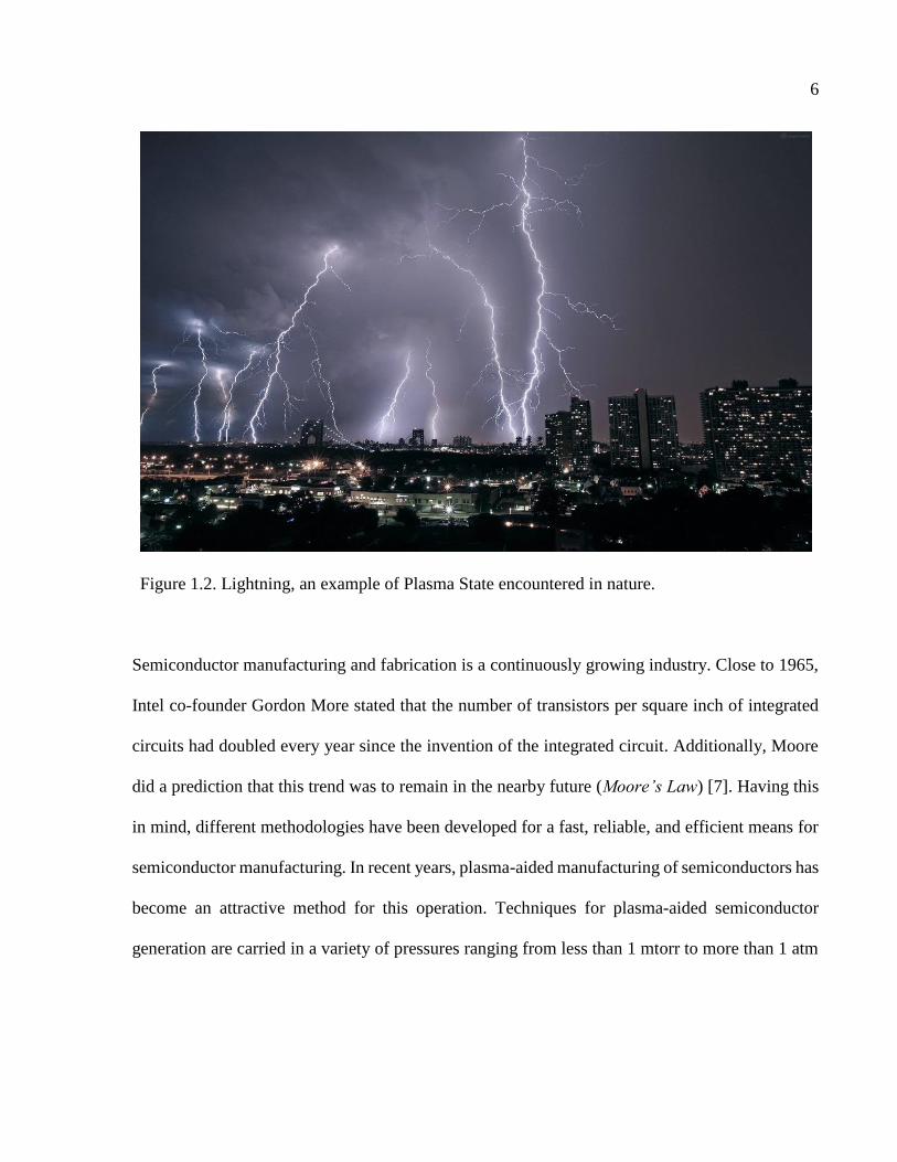
Figure 1.2 Lightning, an example of Plasma State encountered in nature .....................................6
Figure 1.3 Treatment of Tomatoes in a Plasma Chamber ..............................................................8
Figure 1.4 (a) Gliding Arc Plasma Models with Reverse Vortex Flow (b) Gliding Arc Plasma
Chamber Top View ......................................................................................................10
Figure 2.1 Classification of Plasmas .............................................................................................14
Figure 3.1 Generated Mesh Statistics ...........................................................................................32
Figure 3.2 (a) Geometry Model of the Cold Plasma Chamber (b) Mesh Generated for Finite
Element Analysis of the Cold Plasma Chamber .........................................................33
Figure 3.3 Temperature Patch in the Airgap for Cold Plasma Chamber Model ..........................35
Figure 3.4 Current Density Present in the Airgap of the Cold Plasma Chamber Model .............36
Figure 3.5 (a) Simulated Current Through Bottom Electrode (b) Simulated Magnetic Field
Located at the Horizontal Plane of the Airgap .............................................................37
Figure 4.1 Cold Plasma Chamber Prototype.................................................................................40
Figure 4.2 Experimental Setup ....................................................................................................42
Figure 4.3 (a) Experimental Setup: Cold Plasma Chamber with Electromagnetic Probe
(b) Magnetic Field Stable Signal (c) Magnetic Field Saturated Signal .......................43
Figure 4.4 Cold Plasma Chamber During Operation Time .........................................................45
Figure 4.5 Input Voltage Waveform (yellow), Input Current Waveform (pink), Induced Voltage
in Magnetic Field Probe Representing Magnetic Field (green). ..................................46
Figure 4.6 Isolated Induced Voltage Waveform for Magnetic Field Calculation ........................47
Page 10
x
LIST OF TABLES
Table 1.1 Comparison on Different Plasma Technologies ...........................................................11
Table 3.1 Cold Plasma Chamber Model Dimensions ...................................................................31
Table 4.1 Simulated vs. Experimental Results Comparison .........................................................49
Page 11
1
CHAPTER 1
INTRODUCTION
One of humanities longest quests has been the continuous search of means and sources of energy
for their various activities. The realm of activities for which energy has been utilized varies from
means of transportation, to sources of heat, and labor. In the time before the industrial revolution,
which was considered as one of the inflection points of our history, people used to make use of
burning wood as a source of heat generation and light during the time that the sun was not shining.
Combustion engines and machines were yet to be invented, so people used animals to execute the
labor that they were not able to do such as pulling a carriage, or preparing the field for seedtime in
the case of land transportation. Sails and wind provided the motive power for transportation on the
sea. With the discovery of electricity by the 17th century, many inventions arose such as an early
electrostatic generator, the differentiation between positive and negative currents, the classification
of materials as conductors or insulators to mention a few examples. By far one of the most relevant
achievements regarding electricity was attained by Joseph Swan and Thomas Edison who set up a
joint company to produce the first practical filament lamp, which was later used by Edison’s direct
current (DC) system to provide power to illuminate the first street lamps in the New York City at
the beginning of the 1880’s. At the same time that Edison came with his DC system idea, one of
the most iconic scientist in history, Nikola Tesla, proposed an alternating current (AC) system
which would revolutionize power systems and power transmissions for its benefits disregarding
DC systems disadvantages [1]. The proposed system by Tesla consisted of a voltage step-up
Page 12
2
transformer for long distance transmission and then a voltage step-down transformer for residential
power distribution. This system provided an increase in efficiency, as well as cost reduction when
compared side by side with Edison’s DC system.
Having a viable solution for an efficient and considerably cheap power transmission, one issue
remained to be addressed: power generation. Since the start of the industrial revolution coal and
petroleum had been a very attractive mean for generation of power due to their relative easiness to
find and its abundance in the planet. Steam power plants generate their energy by using a burning
agent, usually coal or fossil fuels, to provide a heat source in order to turn water into steam. The
high pressurized steam is then moved through a piping system that will later take it to the blades
of turbines. The movement of this blades will cause giant coils inside the generator to turn.
Consequently, an electric field will be generated which will force electrons to move and thus
starting the flow of electricity. At the time this idea was proposed, scientist did not take into
consideration the fact that coal and fossil fuel were not unlimited resources. Additionally, it was
not foreseen that the abusive use of these sources as means of power generation could effectively
harm the environment. The harm in the environment can be seen as how CO2 emissions contribute
to the emission of greenhouse gases that directly impact the downsize of the ozone layer; which
consequently increase the average temperature of the planet causing natural disasters, a problem
more commonly known as climate change. This cause-effect situation opened a new niche for
researchers known as renewable energies.
The renewable energy research has been widely studied, providing viable solutions for the
problems mentioned above caused by the power and energy generation from fossil fuels. Soon,
energy conversion from natural ‘unlimited’ resources to electricity became a very popular among
Page 13
3
the scientific community. The most known renewable energy resources are energies harvested
from sunlight, water, wind, and geothermal resources. Even though these renewable energy
resources have proven their ability and reliability to provide energy at a large scale, solutions
containing fossil fuels keep being the most used sources for power and energy generation. More
advances need to be achieve in terms of renewable energies so that little by little they become the
greatest suppliers for power and energy generation. Many countries around the globe, including
the United States, have created renewable energy portfolios in which they have set goals to be
achieved in some years regarding specific percentages that renewable energies will provide to the
total generation of electricity.
An important aspect of renewable energy resources is energy storage management. This is due to
the fact that in most of the cases for renewable energies, on demand supply is not available. For
instance, sunlight is only available for certain amount of hours during the day; moreover, in wind
generation of energy, wind will not be always available or present with a constant speed. There
are many methods that have been studied for energy management systems, however hydrogen fuel
cells are currently a very attractive solution for its many advantages compare to other traditional
energy storage methods. The principle of operation of fuel cells is that it is device that converts
chemical energy stored in gaseous molecules from a fuel into electrical energy. In the most
common of cases hydrogen is the preferred fuel used for fuel cells. Hydrogen and oxygen are
combined inside the fuel cell to produce electricity [2]. Figure 1.1 shows the operation
methodology and basic fuel cell structure. This structure typically consists of an electrolyte
membrane which maintains contact with two electrodes: anode and cathode. Hydrogen is fed into
the anode side and oxygen, which acts as an oxidant is fed to the cathode. As a byproduct of this
Page 14
4
chemical reaction in which hydrogen molecules are transformed into electric energy, the process
yields water and heat.
As hydrogen became a very important player into renewable energy systems, researchers have
been trying to find a way to produce hydrogen from clean sources as well as from efficient
processes. Some of these processes are steam reformation, production methods from fossil fuels
such as partial oxidation, plasma reforming, among others, as well as hydrogen production from
water as a fuel in processes such as electrolysis, radiolysis, among others [3]. From the previously
mentioned methods, plasma reforming its one of the most attractive methods for hydrogen
generation purposes.
Figure 1.1. Operation Model of a Hydrogen Fuel Cell.
Page 15
5
1.1 State of the Art
Plasma is considered to be one of the four fundamental states of matter, with the other three being
more commonly known: solid, liquid, and gas. The appellation of “the fourth state of matter” to
reference plasma state was first appointed by English chemist and physicist Sir William Crookes
in 1879 [4]. Originally, this term was used to describe an ionized medium created in a gas
discharge, very similar to that one created by lightings present in thunder storms, like that one
shown in Figure 1.2. Even though the proposed definition for a plasma above is good, it is not
accurate enough. A more useful definition is that plasma is a quasineutral gas of charged and
neutral particles which exhibits a collective behavior. From time to time it has been said that most
of the composition of the universe, about 99%, is in plasma state [5]. This estimate however may
not accurately represent the reality, but certainly it is a very reasonable approximation since stellar
interiors and atmosphere, gaseous nebulae, and much of the interstellar hydrogen are plasmas.
Going back to plasmas present in our own environment, such as lightning bolts more examples
can be given such as: the glow of the Aurora Borealis, the conducting gas inside a fluorescent tube
or neon light, and the slight amount of ionization in a rocket exhaust [6].
Plasmas can be utilized in many industrial applications such as semiconductor fabrication, medical
procedures, materials processing (i.e. food sterilization, disposal of sewerage), and as means of
hydrogen reformation for fuel cell applications, just to mention a few examples of its applications.
Page 16
6
Semiconductor manufacturing and fabrication is a continuously growing industry. Close to 1965,
Intel co-founder Gordon More stated that the number of transistors per square inch of integrated
circuits had doubled every year since the invention of the integrated circuit. Additionally, Moore
did a prediction that this trend was to remain in the nearby future (Moore’s Law) [7]. Having this
in mind, different methodologies have been developed for a fast, reliable, and efficient means for
semiconductor manufacturing. In recent years, plasma-aided manufacturing of semiconductors has
become an attractive method for this operation. Techniques for plasma-aided semiconductor
generation are carried in a variety of pressures ranging from less than 1 mtorr to more than 1 atm
Figure 1.2. Lightning, an example of Plasma State encountered in nature.
Page 17
7
[8]. At high pressures, plasma etching and deposition show advantages due to its combination of
material science, plasma chemical and physical properties [9].
An emerging field within the medical community is the utilization and combination of plasma
physics, life science, and clinical medicine to use physical plasma for therapeutic applications. It
is important to mention that plasma medicine can be categorized in three main areas which are: 1)
Non-thermal atmospheric-pressure direct plasma for medical therapy, 2) Plasma-assisted
modification of bio-relevant surfaces, and 3) Plasma-based bio-decontamination and sterilization.
As discussed in [10] plasma use for medical therapy and treatment of chronic wounds is an
evolving research field for optimized low-temperature atmospheric plasma jet devices.
Additionally, it has been researched that between 5% and 10% of the patients admitted to a hospital
usually acquire healthcare infections. It is important to counter this drastic statistics by making
good use of technology, and for this matter plasma based bio-decontamination and sterilization
methods offer very attractive solutions [11]. The importance of biotechnology and biomaterials in
modern day medicine seems to be rising over the last few decades as technology becomes better.
As biomaterials are implanted in living tissue, a variety of biological interactions start to take place
as close as the first few nanometers of the material surface and the tissue [12]. When this implants
of biomaterials are placed in human tissue protein formation between the layers can produce
implant failure due to bacteria and thrombin formation [13, 14]. For this, and other problems
related to implants of biomaterials, a diverse amount of solutions have been developed among
which plasma modification techniques like ion beam implantation and plasma polymerization [15].
In recent years, food safety has become a major concern in the food industry. With problems
arising from cultivating crops in the field, to contamination by transportation, up to problems due
Page 18
8
to genetically modified organisms different methods have been developed to avoid contamination
and sterilize food. Utilizing plasma discharges at a low temperature and atmospheric pressure
provide a very practical, inexpensive and very suitable solution for the decontamination and
sterilization of food products which most of them are not very heat tolerant [16]. In many of these
applications of food decontamination it is important that the plasma method used is non-thermal
plasma. By using thermal plasma, the extremely high temperatures above ambient can be very
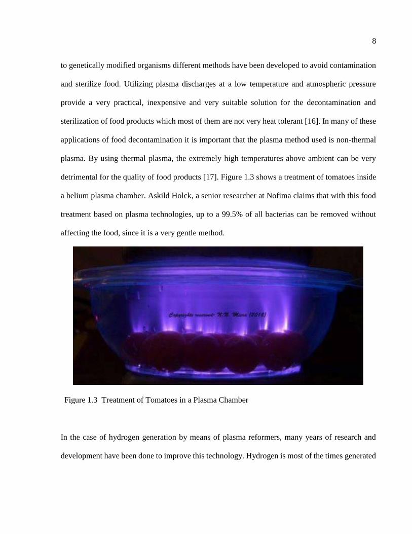
detrimental for the quality of food products [17]. Figure 1.3 shows a treatment of tomatoes inside
a helium plasma chamber. Askild Holck, a senior researcher at Nofima claims that with this food
treatment based on plasma technologies, up to a 99.5% of all bacterias can be removed without
affecting the food, since it is a very gentle method.
Figure 1.3 Treatment of Tomatoes in a Plasma Chamber
In the case of hydrogen generation by means of plasma reformers, many years of research and
development have been done to improve this technology. Hydrogen is most of the times generated
Page 19
9
from hydrocarbons through an oxidation process, most commonly known as hydrogen
reformation. Many methods are available for achieving reformation such as: steam reformation
(SR), partial oxidation (POX), auto-thermal reformation (ATR) or dry CO2 reformation.
Additionally, in order to improve efficiency of the hydrogen generation process, various types of
plasma and geometries have been researched, developed, and studied for different operational
points. Out of all the discoveries, the most noticeable and noble developments include the
Plasmatron by L. Bromberg et al. [18], gliding arc with Reverse Vortex Flow (RVF) by Fridman
et al. [19], gliding arc discharge by A. Czernichowski [20] and plasma torch by Rollier JD [21].
In Figure 1.4 a description of the gliding arc with RVF is shown. As it can be seen from Figure
1.4 (a) it appears that the arc has the appearance of a flame, however it is just one single plasma
arc, at a very high velocity, thus the appearance of a flame. Additionally, it is worth mentioning
how the plasma can fill most of the volume of the reactor. The latter is considered to be one of the
characteristics of the gliding arc design most important features, which makes it a superior design
compared to those before mentioned. Moreover, Figure 1.4 (b) shows the top view of the gliding
arc plasma chamber. It perfectly depicts the reverse vortex flow phenomena that characterizes this
technology.
Page 20
10
(a)
(b)
Figure 1.4 (a) Gliding Arc Plasma Models with Reverse Vortex Flow. (b) Gliding Arc Plasma
Chamber Top View.
Table 1.1 shows a brief comparison on the power, efficiency, and reformation methods of the
above mentioned plasma reformation systems.
Page 21
11
Table 1.1 Comparison on Different Plasma Technologies
H2 Output
(kW)
Efficiency
(%)
Process
Plasmatron
RVF Gliding Arc
Gliding Arc
Plasma Torch
7.14
1.19
6.67
2.8
63.59
75.81
54.28
41.78
ATR
POX
POX
SR
1.2 Motivation and Significance
Design and modeling of any kind of application is a very important part of the research and
development process. The main purpose of this Master Thesis is to provide an insight and a tool
by means of finite element analysis (FEA) of a multi-physics modeling of a cold plasma reformer.
By doing this, it would be a useful working tool for modeling and optimizing purposes for the
design and control of plasma reformers. With this it is intended that more resources are spent
during the research and development phase on the project, and less of it in the prototyping and
validation stage of it. Moreover, a significant amount of studies have been performed regarding
plasma, but nearly none of them have a comprehensive study including thermal, fluid, and
electromagnetic phenomena that occur during the operation of a cold plasma reformer.
Page 22
12
1.3 Summary
This chapter provided a brief introduction to the importance of plasma for multiple industrial
applications, especially the ones dealing with hydrogen production since it can be used for other
applications such as input fuel for fuel cells. The current state of the art for multiple applications
of plasma was discussed as well.
The following chapters of this Thesis will be organized as follow: Chapter 2 covers the physical
fundamental properties that govern the plasma state, including electromagnetic properties,
thermodynamic properties, and transport properties of plasma. Chapter 3 discusses the Finite
Element Modeling of the plasma chamber, including all the assumptions taken into consideration,
as well as a detailed explanation of the simulation modeling for this project. Chapter 4 includes
Experimental Results and Verification of the Finite Element Model discussed in Chapter 3. Finally,
Chapter 5 contains Conclusions and Recommendations based on the research performed in this
Theses. Lastly, an appendix is included with significant mathematical derivations, and lines of
code for the simulation part of this Thesis.
A conference paper in the topic has been accepted for publication in the 17th Biennial Conference
on Electromagnetic Field Computation (CEFC 2016), the paper has been cited in [22]. Some of
the results of this paper will be shared in this thesis.
Page 23
13
CHAPTER 2
PHYSICS FUNDAMENTALS OF THERMAL PLASMAS
Plasma physics play an important role in design, modeling and simulation of the fourth state of
matter. For many years, scientist have research and developed the physics rules and fundamentals
that govern all theory regarding plasma interactions with itself and with its medium. The physical
properties of plasma will be dependent upon what type of plasma is generated. The main focus of
this thesis will be regarding thermal plasmas, for that reason, in Section 1 of this chapter a brief
summary of the types of plasmas will be described. Section 2 presents general properties of the
composition of thermal plasmas. Additionally, in Section 3 thermodynamic properties of thermal
plasmas will be presented. Section 4 will take into consideration the transport properties present
in thermal plasmas. Finally, Section 5 will present electromagnetic properties that will be
explained as a function of plasmas.
2.1 Different Plasma Types
One of the most basic categorization of plasmas can be the following: natural or man-made. As
the name suggests natural plasmas are the ones present in the universe, naturally. The most
common examples of plasmas that occur naturally are lightning strikes and the aurora borealis.
Both phenomena are known to occur at a both high and low pressures. By having such differences
in the pressure that the plasma occurs, a significant difference in their aspect can be seen. Thus it
Page 24
14
is concluded that pressure of plasma can affect not only its luminosity or intensity, but also the
energy that the plasma will carry, thus affecting as well its thermodynamic state.
Since plasmas can exist in a variety of pressures, it has been determined that a good way to classify
them is based on their electron temperature and electron density. Figure 1 shows an example on
the classification of plasmas based on their electron density and electron temperature.
Figure 2.1 Classification of plasmas.
Page 25
15
2.2 Thermal Plasmas
Since the main focus of this thesis will be thermal plasmas a clear distinction between thermal and
non-thermal plasmas need to be made. Depending on which part of the world you are from, thermal
plasmas can be considered as “hot plasmas” in the European and American literature, and as “low
temperature” in the Russian literature. However, what it is clear is that plasma can be considered
thermal as long as it is in or close to Local Thermodynamic Equilibrium (LTE). An additional
condition for a plasma to be considered thermal is that excitation (kinetic) and chemical
equilibrium within the particles should exist as well. The before mentioned conditions are of such
importance that it has been discovered that it is quite difficult to find a plasma in total LTE. Many
deviations exist such that even though they are not in LTE, they are still considered thermal
plasmas, just that in Partial Local Thermal Equilibrium (PLTE). In contrast, when the kinetic and
chemical equilibrium are not met within the particles of the plasma, it is considered to be a non-
thermal plasma. Since equilibrium does not exist in non-thermal plasmas, some of the causes of
this is the temperature difference from the ions with respect to the electrons, or because the velocity
distribution of one of the present species of the plasma does not follow the Maxwell-Boltzmann
distribution.
It is known that the kinetic temperatures in plasma, as well as in any gaseous medium, are function
of individual particle, such as molecule, atom, ion, or electron, average kinetic energy.
1
2𝑚𝑣2 =
3
2𝑘𝑇 (1)
where m is the particle mass, (v2)1/2 is the effective velocity of the particle, k is the Boltzmann
constant, and T represents the absolute temperature. Equation (1) then implies that a Maxwell-
Boltzmann distribution is followed by the particle, which as a result can be expresses as:
Page 26
16
𝑓(𝑣) =4
√𝜋(
2𝑘𝑇
𝑚)
3
2𝑣2 exp (−
𝑚𝑣2
2𝑘𝑇) (2)
The Maxwell-Boltzmann distribution expressed in Equation (2) is going to be dependent on how
the particles will interact among each other. These interactions can be measured by the frequency
of the collisions, and on the exchanged amount of energy during a particular collision.
Additionally, the energy transferred from an electron to a heavy particle in a single collision can
be expressed as the following:
3
2𝑘(𝑇𝑒 − 𝑇ℎ)
2𝑚𝑒
𝑚ℎ (3)
where Te and Th represent the electron and the heavy particle temperature, respectively. With this
been said, it is clear that as long as the temperatures of the electron is much higher than that of the
heavy particle ( Te>>Th ) then there is a deviation from kinetic equilibrium of the plasma and thus,
the plasma will be non-thermal.
An additional, yet important condition for a plasma to be considered thermal is that the range of
pressure in which it exists is above 1kPa. With pressures above 1kPa, electron temperature as well
as heavy particles temperature converge to an almost equal temperature, thus ensuring that the
plasma maintains the LTE condition.
The following sections of this chapter will discuss some of the main characteristics and properties
of thermal plasmas, including thermodynamic, transport, and electromagnetic properties, as well
as conservation of energy and mass.
Page 27
17
2.3 Thermodynamic Properties
It has been repeatedly said that plasma is a collection of a considerable amount of charged particles
moving in a medium. Let’s consider the simplest many-body system of non-interacting point
particles: and ideal gas. It is known that the ideal gas has an equilibrium statistical mechanics
equation that follows:
𝑃 = 𝑛𝑘𝑇 (4)
where P is the pressure, n is the density of the particles, k is the Boltzmann constant, and T the
absolute temperature.
2.3.1 Plasma Parameter
However, from previous discussion, plasma cannot be considered an ideal ionized gas, thus it is
impossible to determine all the thermodynamic properties of it without the aid of a small parameter
that describes up to a certain point all the deviations of the non-ideal system from that one that is
ideal. This small parameter is the ratio of the mean distance of closest approach to the average
spacing between the particles within the plasma.
The plasma parameter, represented by g, is defined by
𝑔 = (8𝜋𝑒2
𝑘𝑇)
3
2𝑛0
1
2 (5)
where n0 is the distance between particles in the medium. Additionally, equation 5 can also be
expressed in terms of the Debye length
𝜆𝐷 = (𝑘𝑇
8𝜋𝑛𝑒2)
1
2 (6)
Page 28
18
finally, the plasma parameter can be expressed by means of Debye length as in Equation 7. The
Debye length is a measure of the sphere of influence of a given test charge in the plasma.
𝑔 =1
𝑛0𝜆𝐷3 (7)
In other words, equation 7 explains the reason as of why the plasma approximation can be called
“many particles in a Debye sphere”. If there are many particles present within the Debye sphere,
then the plasma parameter will be small, and thus the average potential energy of a plasma particle
is much less than its average kinetic energy. Thus in general, the plasma parameter tells the amount
of plasma particles in a Debye sphere.
2.3.2 Specific Heat at Atmospheric Pressure
One of the most important thermal properties in plasma is specific heat cp. By definition, specific
heat is:
𝑐𝑝 = (𝜕ℎ𝑔
𝜕𝑇)
𝑝 (8)
where hg is the specific enthalpy of the system, and the specific heat of the system is evaluated at
atmospheric pressure (1 atm). The specific enthalpy of the system can as well be defined as
ℎ𝑔 =∑ 𝑥𝑖𝐻𝑖
𝐾𝑖=1
∑ 𝑥𝑖𝑀𝑖𝐾𝑖=1
(9)
where xi, Mi, and Hi are the molar fraction, the mass of one mole, and the enthalpy of one mole of
the chemical species under study respectively.
Page 29
19
2.3.3 Enthalpy and Entropy
Moreover, enthalpy and entropy are very important thermodynamic properties in plasma. In a
general sense, enthalpy can be defined as a thermodynamic quantity equivalent to the total heat
content of the system. In other words, it can be expressed as the total internal energy of the system
plus the product of pressure and volume of the system itself.
𝐻 = 𝑈 + 𝑝𝑉 (10)
where H is the enthalpy of the system, U is the internal energy of the system, and pV is the product
of the internal pressure with respect to the enclosed volume of the system. Moreover, the Entropy
of a system, in a general way can be defined as a thermodynamic quantity that represents the
unavailability of a systems thermal energy for conversion into mechanical work:
𝑆 = 𝑘𝑙𝑛(𝛺) (11)
where S is the entropy, k is the Boltzmann constant, and is the then number of microscopic
configurations that correspond to such thermodynamic system. Even though those were very
general definitions for these properties, they will help to build up the concept of Enthalpy and
Entropy applied for thermal plasmas.
The functions of entropy and enthalpy for plasmas can be calculated perfectly by directly deriving
equation 9, or by integrating over the specific heat as follows:
ℎ𝑔 − ℎ𝑔0 = ∫ 𝑐𝑝(𝑇)𝑑𝑇
𝑇
0 (12)
where hg is the total enthalpy of the chemical at a specific temperature and specific pressure,
whereas hh0 is the total enthalpy of the chemical at a temperature of 0 degrees Kelvin and 1
atmosphere of pressure.
Page 30
20
Even though these are very important thermodynamic properties, in many years of research tables
have been developed so that these values are easily available for calculations. Tables for density,
specific heat, enthalpy, entropy, viscosity, thermal and electrical conductivity can be found in
Appendix A for reference an example of variations of these properties with respect to temperature,
and chemical compositions.
2.4 Transport Properties
In the vast majority of transport processes, a linear relationship exists between the flux and the
driving force of such processes. In a very general way:
𝑓𝑙𝑢𝑥 = 𝑐𝑜𝑒𝑓𝑓𝑖𝑐𝑖𝑒𝑛𝑡 𝑋 𝑑𝑟𝑖𝑣𝑖𝑛𝑔 𝑓𝑜𝑟𝑐𝑒
this type of relationship is also called a phenomenological law (Ohm’s law for electricity is a clear
example of this law). In the specific case of plasma transport equations and properties the following
are the most notorious cases and examples:
𝐽𝑛 = −𝐷𝛻𝑛 (13)
where Jn is the flux density of an amount of particles n, and D is the diffusion coefficient expressed
in m2/s;
𝐽𝑝𝑥= −𝜇
𝑑𝑣𝑥
𝑑𝑧 (14)
where Jpx is the flux density of the momentum of the plasma (in this particular case in the X
direction), and is the viscosity expressed in kg/m;
𝐽𝐸 = −𝜅𝛻𝑇 (15)
where JE is the flux density of energy of the plasma, and is the thermal conductivity expressed
in W/mK;
Page 31
21
𝐽𝑒 = 𝜎𝑒𝛻𝑉 (16)
where Je is the charge flux density of the plasma, e is the electrical conductivity expressed in
mho/m, and it is important to note that -𝛻𝑉 is the Electric Field present in the thermal plasma.
For simulation purposes that will be later explained more in detailed in Chapter 3, one of the most
relevant and important transport coefficients is the electrical conductivity. In thermal plasmas,
electrical conductivity is a property highly dependent of temperature. In a simplified derivation of
the transport coefficients presented in [23] was stablished that
𝜎𝑒 = 𝑒𝑛𝑒𝜇𝑒 (17)
with
𝜇𝑒 =𝑒𝑙𝑒
√𝜋𝑘𝑇𝑚𝑒 (18)
From the Maxwellian distribution, a first approximation is made for le
𝑙 =1
√2𝑛𝜎0 (19)
thus, combining the two equations above
𝜎𝑒 =𝑛𝑒𝑒2
√2𝜋𝑇𝑚𝑒𝑛𝑎𝜎𝑒𝑛 (20)
where, ne is the density of electrons, e is the electron charge, me is the mass of the electron, na is
the neutral particle number density, and en the electron-neutral collision cross section.
Hence from the expression for electrical conductivity above it can be said that it highly depends
mainly on electron density and varies almost in an exponential fashion with respect to temperature.
With this it is understandable as why electrical conductivity is almost negligible in all common
gases used for plasma purposes at temperatures below 6000K (see appendix A to check the table).
Page 32
22
2.5 Electromagnetic Properties
It has been widely studied the effects that different applications have in the generation of electric
and magnetic fields, and thermal plasmas have not been the exception.
2.5.1 Maxwell’s Equations
Electric and magnetic fields present in thermal plasmas exist and are governed by Maxwell’s
equations. There exist 4 Maxwell’s equations that can be found separately throughout history.
They were discovered by many scientists and mathematicians such as Charles-Augustin Coulomb,
Jean Baptist Biot, Felix Savart, Andre Ampere, Michael Faraday, among others. But it was James
Maxwell in 1861, who ingeniously integrated all those laws relating electricity and magnetism that
at a first glance appeared to be unrelated. Hence the name ‘Maxwell Equations’.
Assuming that the ionized charged particles of plasma occur in vacuum, according to Maxwell’s
equations, the following applies:
∇ ∙ 𝐸 =𝜌
𝜖0 (21)
𝛻 × 𝐸 = −𝜕𝐵
𝜕𝑡 (22)
𝛻 ∙ 𝐵 = 0 (23)
𝛻 × 𝐵 = 𝜇𝑜 ( 𝐽 + 𝜖0𝜕𝐸
𝜕𝑡) (24)
where is the charge density in the plasma, J is the current density in the plasma, and 0 and 0
are the permittivity and permeability of free space, respectively. It is important to note that the
charge density and the current density comprise all the currents and all the charges of all the
particles species present in the plasma stream.
Page 33
23
The above mentioned equations will be further discussed in Chapters 3 and 4 when explaining how
all simulations were performed, as well as how the calculations were done.
2.6 Summary
Fundamentals of plasma physics have been described and equations have been developed and
derived throughout this chapter. Additionally, important physical properties of plasma have been
explained as well as their importance.
Page 34
24
CHAPTER 3
STEADY STATE ANALYSIS OF COLD PLASMA CHAMBER
Steady state analysis and simulations of the cold plasma chamber will provide steady state
information of the multiple phenomena happening simultaneously when the chamber is in normal
operation mode, such as current density, current, magnetic field, among others. These parameters
are later going to be used to compare and verify the accuracy of the finite element model with
respect to actual experiments. The above mentioned results will be discuss in detail in Chapter 4.
For simulation results, Numerical Analysis method has been performed using the benchmark
software Ansys 17.0. Section 3.1 briefly describes the theory behind the numerical analysis. In
Section 3.2 the specific assumptions taken in order to build the model are presented. Section 3.3
describes the user defined function (UDF) that was implemented in order to run the simulations.
Last but not least, Section 3.4 presents simulation details and results that will be later compared
with experimental results.
3.1 Finite Element Analysis Method
The finite element analysis (FEA) method has been developed and verified by many researchers
for all different sorts of applications. FEA is a numerical analysis and computational tool and
technique in which an approximate solution to a boundary value problem for sets of partial
differential equations is achieved. FEA basically takes a large scale problem and divides it into
smaller and simpler parts called finite elements in which the studied problem is analyzed. The
Page 35
25
results of each individual finite element is then evaluated and combined to get the total
approximate result of the whole body under study. The FEA method uses variation methods from
calculus to approximate a solution by making the error of the associated function as minimal as
possible.
In order to perform an accurate calculation and solution using the FEA method, a correct geometric
representation of the model and complex geometry under study needs to be made. Moreover, a
correct representation of the material properties of the materials of the model need to be included
so that the model is valid. Additionally, a variety of assumptions and simplifications of the system
need to be made so that computational time is acceptable, yet the solution will still be valid.
Finite element analysis method can be completely understood as a computational tool for
performing engineering analysis of complex problems that need to be further understood. By
making use of this tool, the generation of a complex mesh is necessary to subdivide the large
geometry into smaller sections (as stated in the previous paragraphs) in which the set of partial
differential equations that are associated with the problem under study will be analyzed. In the
particular case of cold plasma applications, the Navier-Stoke equations are analyzed to understand
what happens when the arc occurs between two electrodes. Further explanations as in how these
equations are analyzed by FEA will be given later in this chapter, as well as all the assumptions
made to simplify the problem will be explained.
A wide variety of software are used for finite element analysis and are available in the market,
however all the simulations performed in this thesis have been done in benchmark software from
Ansys 17.0. It is important to explain that at least 4 different software’s have been used to compute
the different results. For instance, Ansys Maxwell 17 was used to compute the magnetic and
Page 36
26
electric field, as well as the Lorentz forces due to plasma arcs. Moreover, Ansys Fluent 17 was
used as a mean to compute the computational fluid dynamics of the system, since flows,
temperatures, and other properties were taken into consideration is this multiphysics study.
3.2 Assumptions and Estimations
In this section of the thesis the assumptions and estimations taken into consideration in order to
model the cold plasma chamber will be discussed. As it was stated in Chapter 2, there exists two
different type of plasmas: thermal and non-thermal. This distinction is very relevant to this matter
since the properties that will be given to the FEA simulation software will come from defining our
problem as a thermal or non-thermal plasma. Additionally, this will give place to assumptions
regarding the interactions of the plasma by itself with the medium and with the other materials that
will be part of the model, such as the electrodes that will carry the high voltage to ionize the
medium so that the arc takes place.
The most important assumption for simulations purposes only is that the plasma is thermal plasma.
It was discussed in Chapter 2 that cold plasma and plasma arcs and streamers were considered
non-thermal plasmas. However, in this thesis it has been assumed that only one period of the arc
frequency is going to be considered, and that at that instant of time the plasma will be thermal and
will be in local thermal equilibrium (sufficient and necessary condition to consider a plasma to be
thermal).
A benefit of considering the plasma to be thermal, is that we know most of its properties and
behavior since it has been widely studied for many years. For instance, this assumption lets us
consider that both electron and particle temperatures are the same, so they can be treated as one in
Page 37
27
the FEA simulation. Additionally, the arc is considered to be steady, and there exists axis-
symmetry with respect to the axis parallel to the arc direction. Based on these assumptions the
conservation equations can be maintained.
As it has been mention before, Local Thermal Equilibrium has been assumed for simulation
purposes. What this means is that there are some characteristics of the plasma arc that have been
assumed to be in LTE for simplification purposes. Additionally, this assumes that the arc is in
steady state, no transients are considered in the formation of the plasma arc. It is only considered
a steady arc that happens between the two electrodes. The following conditions must be met
simultaneously in order to consider the plasma to be in local thermal equilibrium:
The different species that form the plasma have a Maxwellian distribution.
E/p is small enough and the temperature within the plasma is sufficiently high that
Te = Th. Where Te is the electron temperature, Th is the heavy species temperature, E is the
Electric Field, and p represents the total pressure of the system. In other words, the
temperature within the plasma is uniform.
Collisions are the dominating mechanism for excitation (Boltzmann Distribution) and
Ionization (Saha Equilibrium).
Spatial variations of the plasma properties are sufficiently smalls. In other words the
gradients of the plasma properties (temperature, density, heat conductivity, electrical
conductivity, etc.) need to be sufficiently small that a given particle that diffuses from one
location to another within the plasma arc will have enough time to reach equilibrium.
Interactions of the plasma with the walls of the chamber will not be considered due to simulation
and computational times. By including these interactions, the analysis of the problem will become
Page 38
28
very difficult to reach convergence. Additionally, the more complicated the FEA is setup, the more
chances for simulation errors and it will be harder to match the experimental results. Moreover,
the fluid dynamics of the system will be considered to be those of a system with laminar and
incompressible flows. This assumption is necessary and justified due to the low Mach numbers of
the fluid in plasma. Furthermore, gravity and heat dissipation due to viscosity effects are very low,
negligible in fact.
Since one of the main goals of this thesis is to investigate how the magnetic field generated by the
plasma arc, only that magnetic field will be considered. In other words, the thermal plasma arc will
not be affected by any other external magnetic field created by permanent magnets, for instance.
Lastly, it has been assumed that since plasma is in local thermal equilibrium the whole study will
be performed at steady state conditions. Thus, no transients have been considered for this analysis,
unless it has been stated for some simulations and comparisons.
3.3 User Defined Functions and Simulation Implementation
A lot of challenges are presented when it comes to multiphysics studies for phenomena such as
plasma. Plasma itself, been a non-linear phenomenon is very difficult to characterized. Not only it
is very difficult to characterize plasma, but also the combination of the multiple interactions that
take place at the same time is hard to implement. For this same reason, mainly two software
packages provided by Ansys were used: Fluent 17 and Maxwell 17 to study the cold plasma
chamber.
The reason on why the software was chosen is very simple. Maxwell provides the capability of
calculating and performing the FEA and return results of magnetic field, as well as current density.
Page 39
29
On the other hand, Fluent allows to perform the Computational Fluid Dynamics (CFD) study to
plasma in a way that it would allow the plasma arc to be modified by the temperature of the
particles of the plasma. However, the two processes and calculations above mentioned are separate
and isolated. In other words, both Maxwell and Fluent would perform both calculations separately
without taking into account the effects that one might have on the other one. As it has been
discussed previously, the conductivity of a thermal plasma is highly dependent on the temperature
of the ionized particles that carry the charge of the plasma. Thus, if the temperature of the
conduction path or ionized particles changes in fluent due to its fluid dynamics properties, those
changes would not be reflected in the electromagnetic result provided by Maxwell.
Hence, the necessity of creating a link between the two software mentioned was present. Ansys
allows users to create user defined functions (UDF) so that by means of coding you can go more
in depth into the software so that your problem is defined as accurately as possible. A UDF is a
routine written in C-language which can be dynamically linked with the solver of your FEA. By
creating the UDF customization of boundary conditions, source terms, reaction rates, material
properties, among other things can be modified since the standard interface cannot be programmed
to do regularly.
The basic steps to create a UDF to be used in Fluent consist of creating a file containing the source
that tells the software what operations will be performed, as well as the material properties that
will be modified. Interpretation and compilation of the UDF will be necessary to be performed
through the software. Assign the changed values and parameters that have been modified by the
UDF to those in the software. And lastly you need to run the calculation.
Page 40
30
The UDF that was coded for this thesis works in the following way: Maxwell is called by Fluent
as a function in order to calculate magnetic field and current density distribution based on the
temperature dependent conductivity that is updated by Fluent. In other words, Fluent was run and
depending on the initial conditions, and how the flow interacted with the model, temperature
changed in the area where the arc happens. The temperature was matched to a lookup table which
contained information regarding electrical conductivity. Once the new conductivity of where the
arc occurred was in a file, that information was sent to Maxwell so that it could process the new
set of boundary conditions and thus calculate magnetic field. Once Maxwell calculated magnetic
field, that information was sent to the Fluent Case and Data file, so that the results could later be
studied and post-processed.
More information regarding the process of performing the simulation will be provided in the
following section of this chapter. Additionally, an excerpt of the UDF is included in Appendix B
at the end of the thesis.
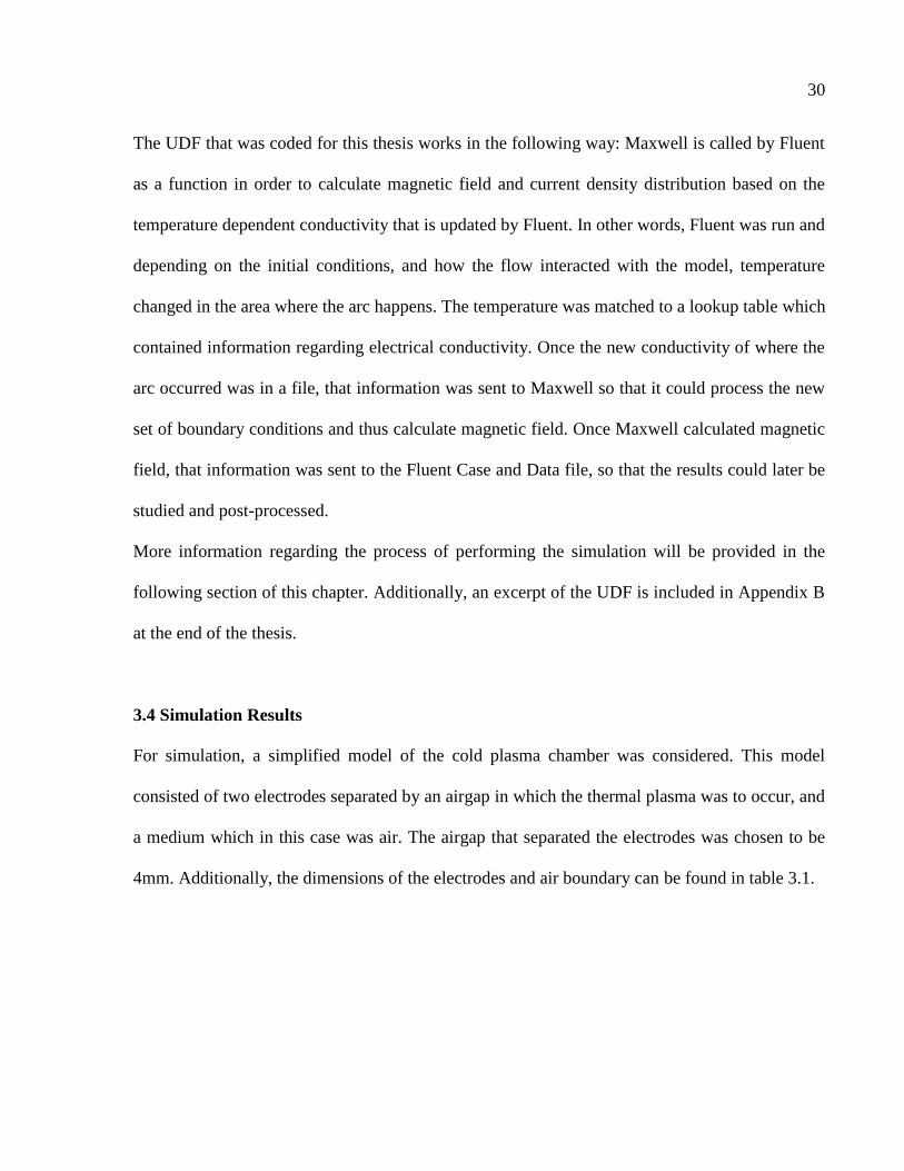
3.4 Simulation Results
For simulation, a simplified model of the cold plasma chamber was considered. This model
consisted of two electrodes separated by an airgap in which the thermal plasma was to occur, and
a medium which in this case was air. The airgap that separated the electrodes was chosen to be
4mm. Additionally, the dimensions of the electrodes and air boundary can be found in table 3.1.
Page 41
31
Table 3.1. Cold Plasma Chamber Model Dimensions
Geometry Size
Top Electrode Height 56mm
Top Electrode Inner Diameter 1.45 mm
Top Electrode Outer Diameter 1.60 mm (1/16 inch)
Bottom Electrode Height 56mm
Bottom Electrode Inner Diameter 5.85 mm
Bottom Electrode Outer Diameter 6.35 mm (¼ inch)
Air Diameter 150 mm
The geometry described above has been used for both Maxwell and Fluent simulations. However,
in order for Fluent to process and analyze the simulation, a mesh needed to be created. As stated
at the beginning of the chapter, FEA method uses smaller geometries or elements to perform
specific tests and analysis regarding the problem, and then after having the results of every single
element in combines them and provide the total result. The mesh for this application needed to be
very small and specific to the area in which the arc occurs in order to capture all the information
necessary to post-process the results, and so that the accuracy of the results was better. There was
a tradeoff in this case, since the smaller the mesh, the more elements the program needed to
compute, and thus incrementing the computational time of the simulation. Figure 3.2 (a) shows
the profile of the geometry that was used for the simulation, and Figure 3.2 (b) shows the mesh
profile of the model. As it can be seen from Figure 3.2 (a) the top electrode is green, and the bottom
Page 42
32
electrode is the orange electrode in the bottom. The surrounding area is the designated area for air,
in other words it is the medium in which the plasma arc will occur. Moreover, Figure 3.2 (b) shows
a cross-sectional screenshot of the mesh that was used for the finite element analysis method. It is
a zoomed in version so that all the details of the mesh can be seen. Additionally, in order to ensure
the validity of the simulations results, an initial check in the mesh generated needed to be made.
A too coarse mesh will not yield good enough results. In order to check this, it was necessary to
take a look at the skewness of the simulation. Figure 3.1 shows the statistics of the mesh generated
for this simulation. As it can be seen, the skewness of the mesh does not go over 0.9. With this, it
is safe to say that the generated is appropriate and simulation can proceed.
Figure 3.1 Generated Mesh Statistics.
Page 43
33
(a)
(b)
Figure 3.2 (a) Geometry model of the cold plasma chamber. (b) Mesh generated for finite
element analysis of the cold plasma chamber.
Page 44
34
The voltage applied between two electrodes increases the temperature of the surrounding medium
changing conductivity, causing ionization, and eventually resulting in occurrence of plasma.
During the instant of plasma formation, a significant drop in voltage and rise is current can be
observed, resulting in generation electromagnetic field. This phenomenon can be described by
using Biot-Savart law
𝑩 = 𝜇0
4𝜋 ∭
𝑣
𝑱(𝑟′)𝑑𝑉′ ×𝒂𝑹
𝑹2 (25)
where B is the magnetic flux density vector, J is the current density vector, R is the distance vector,
and aR is the position vector.
Current density heavily depends on the plasma characteristics, which in turn relies on several factors
such as potential difference, temperature, conductivity, flow rate, and composition of the medium. A
complete electromagnetic simulation of plasma is achieved by operating Maxwell with Fluent
simultaneously as described in Section 3.3 with the user defined function (UDF). Fluent is a multi-
physics simulation tool which includes fluid dynamics, thermal, and electric analysis. Fluent changes
temperature and conductivity of the area between the two electrodes corresponding to the potential
difference, consequently resulting in current flow through the gap. The process is coupled with
Maxwell which generates corresponding magnetic field, hence enabling a complete electromagnetic
simulation of plasma.
Page 45
35
An important simulation aspect is the initial conditions of it. For plasma arc simulations, it is known
that high temperature of the medium is required for the medium to be conductive so that the arc can
take place. However, if no initial conditions are given to the medium where the arc is supposed to
happen, the simulation time will increase exponentially. For this reason in the User Defined Function
there is a temperature patch that defines the region at which the arc will happen and initializes the
temperature of that part setting it at a specific range of temperature to help the simulation time and
convergence of it. Figure 3.3 shows a snapshot of the temperature patch used in the simulation in the
area where the arc will happen.
Figure 3.3 Temperature Patch in the Airgap for Cold Plasma Chamber Model.
Page 46
36
As a result of the temperature patch described in Figure 3.3, the medium for the arc to take place has
been charged to the corresponding electrical conductivity. One way of verifying that there is an arc
present in the simulation is by analyzing the current density of the arc. In Figure 3.4 a snapshot of
the current density in the airgap between the two electrodes has been taken. As it can be seen, current
density is present in the airgap, which tells us that there is a plasma arc present in the cold plasma
chamber model.
Figure 3.4 Current Density Present in the Airgap of the Cold Plasma Chamber Model.
Page 47
37
(a)
(b)
Figure 3.5 (a) Simulated Current Through Bottom Electrode. (b) Simulated Magnetic Field
located at the horizontal plane of the airgap.
Page 48
38
The simulation results for current through the bottom electrode and electromagnetic field on the
horizontal plane located at the center of the electrode gap is presented in figure 3.5 (a) and figure 3.5
(b) respectively.
As it can be seen from figure 3.5 the results for current through the bottom electrode is calculated
to be 36.51A. In order to calculate the value of the average current flowing through the bottom
electrode it was necessary to make a post-processing analysis of the results. First of all, the effective
surface area of the cross-section of the electrode was calculated to be 16.0116*10-6 m2. Since the
current density of the system is given by simulation, an average of the total current density
throughout the electrode was made and later multiplied with the surface area, hence the result of
the average current through the bottom electrode is to be 36.51A.This result will later be compared
to experimental results to verify the validity of our simulation model. Additionally, magnetic field
was calculated from Ansys Post-Processing tools to be 11.48mT. This calculation was done at a
location of 10cm away from the center plane of were the arc is happening. The reason of the 10cm
lies in our experimental setup and the measurement equipment available in the laboratory.
3.5 Summary
In this chapter, the Finite Element Analysis method was explained. Additionally, the simulation
setup for the cold plasma chamber was introduced. User defined functions and how they were
implemented in this simulation was explained. Finally, simulation results were presented. In the
next chapter, experimental results are visited and compared to the results from Chapter 3.
Page 49
39
CHAPTER 4
EXPERIMENTAL RESULTS AND VERIFICATION
Validation of any proposed model is a very important aspect of any research. It is very critical to
make sure that results obtained through calculations and simulations do actually concur with actual
performance of the system. In Chapter 2 a brief introduction of plasmas physics was given.
Additionally, in Chapter 3 a model of a simplified cold plasma chamber was built for simulation
purposes. In Chapter 4 an experimental model has been built in order to validate and compare the
results with those gotten from simulations. Hence, the procedures for the experimental setup and
results are explained in this chapter. Section 1 of this chapter presents the built prototype of the
cold plasma chamber. Additionally, Section 2 shows the operation of the test bed of the cold
plasma chamber, including all operational and measurement equipment. Moreover, Section 3 gives
a detailed analysis of the experimental results, and compares them to those gotten from simulation
results.
4.1 Cold Plasma Reformer Prototype Description
Cold plasma chamber consists a very simple design. First it has two electrodes. The top electrode
has an outer diameter of 1/16th of an inch, whereas the bottom electrode has an outer diameter of
1/4 of an inch. Additionally, it is relevant to mention that the area where the arc happens is enclosed
by a glass with outer diameter dimension of 1 inch. The electrodes are separated by an airgap of
4mm. More details regarding the chamber prototype can be seen in Figure 4.1.
Page 50
40
Figure 4.1 Cold Plasma Chamber Prototype.
4.2 Experimental Setup and Operations
For the experiment the following equipment was utilized:
1. Waveform generator (Agilent 33500B Series) in order to create a voltage pulse with 6V
Amplitude at 2 kHz frequency and 5% duty cycle.
2. High voltage amplifier (TREK model 20/20C-HS) to amplify the input signal at a high
enough voltage level to ionize the medium and make the plasma arc happen.
Page 51
41
3. Anechoic chamber (ETS-LINDGREN model 5240-36) to shield the oscilloscope form any
electromagnetic interference so that the measurements gathered in the oscilloscope were
not affected by any EMI present due to the plasma arc.
4. Digital Phosphor Oscilloscope (Tektronix DPO7254C) for fast acquisition of voltage and
current signals generated by the plasma arc.
5. High voltage probe (Tektronix P6015A) to measure the voltage on the cold plasma
chamber at the time the arc takes place.
6. Current probe (Tektronix A622) to measure the current generated by the plasma arc
flowing through the cold plasma chamber.
7. 100B EMC magnetic field probe (Beehive) with a small loop that offers the best partial
resolution and high frequency response of the available magnetic field probes. This probe
yielded induced voltage information, that was later used to calculate the produced magnetic
field by the plasma arc at different distances from where the arc was happening.
8. Optos Series high pressure liquid metering pump Model 2 (Eldex) in order to pump the
used fuel into the cold plasma chamber for hydrogen reformation purposes.
9. Cirrus ™ 2 benchtop atmospheric pressure gas analysis system that offer the versatility of
state of the art quadrupole mass spectrometry in a convenient bench-top configuration. This
system is used to analyze the chemical composition of the syngas produced by the cold
plasma chamber; more specifically the main interest of this is to investigate the hydrogen
content of the syngas that could possibly be used later as fuel for fuel cell systems.
As it can be seen in Figure 4.2 the experimental setup is shown. One of the important clarifications
that need to be made is that the oscilloscope is inside the EMI shieling chamber since the fast
Page 52
42
changing arcs will produce enough electromagnetic interference to influence the electronics within
the oscilloscope and affect the signal integrity of the waveforms.
Figure 4.2 Experimental Setup.
Choosing which magnetic field probe was very challenging due to the fact that at a certain distance
some of the probes would not capture the magnetic field information whereas in other conditions
(if the probe was too close to the magnetic field source) the probe would easily saturate. For that
reason the small probe was chosen at a distance of 10cm away from where the plasma arc was
happening. With this, stability and integrity of the signal representing the magnetic field generated
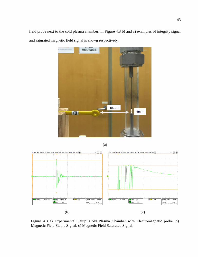
by the arc can be guarantee. Figure 4.3 a) shows the experimental setup for the chosen magnetic
Page 53
43
field probe next to the cold plasma chamber. In Figure 4.3 b) and c) examples of integrity signal
and saturated magnetic field signal is shown respectively.
(a)
(b)
(c)
Figure 4.3 a) Experimental Setup: Cold Plasma Chamber with Electromagnetic probe. b)
Magnetic Field Stable Signal. c) Magnetic Field Saturated Signal.
Page 54
44
From Figure 4.3 b) and c) it can be seen that the correct choice of the magnetic field probe is
important so that the right measurement of Electro Magnetic Interference is seen. Additionally, it
is imperative to mention that the magnetic field probes do not yield magnetic field information. In
turn, it provides induced voltage information that is later processed by calculations to get magnetic
field information. This procedure will be explained later in this chapter when discussing the results.
As seen in Figure 4.2 the system includes a pump to feed the fuel to the system that will be used
for the reformation process using the cold plasma chamber. This feedstock system will feed
Ethanol (in the case of this experiment) or it can feed any hydrocarbon so that syngas is produced
by disintegrating the chemical mixture and that will be later analyzed by the mass spectrometer.
Moreover, in Figure 4.2 is not clear but the whole system includes 2 water traps and 1 water filter,
that can be thought off as filter that will remove any fluid so that only syngas goes to the analysis
in the mass spectrometer.
Additionally, experimentally it was found that due to the long dimension of the high voltage lead
many parasitic inductances and capacitances were added to the system. This was seen by
comparing the rising time specified in the specification sheet of the amplifier to that rising charge
time of the voltage in the cold plasma chamber. At first, the cable was lying on the floor surface
and it caused a delay in the rising charge time. However, it was seen that the interaction that the
cable had with the ground was causing the additional parasitic capacitances and thus more charging
time. This problem was fixed by elevating the high voltage cable from the wall and avoiding any
type of loops that might create additional parasitic inductances.
Page 55
45
4.3 Experimental Results
The experimentally collected results are presented in the following paragraphs of this section. The
cold plasma chamber was run with an input square pulse voltage of 6V0-pk at a frequency of 2 kHz
and duty cycle of 5%. That input voltage was fed to the linear amplifier that was not limiting the
current, so it was operating at 100% current flow to the cold plasma chamber. Figure 4.4 shows a
snapshot of the cold plasma chamber during operation time.
Figure 4.4 Cold Plasma Chamber during operation time.
As it can be seen in Figure 4.4, the ionized medium between the two electrodes becomes
conductive as the temperature of the particles is increased and its electric conductivity is enough
Page 56
46
for current to flow through the path of shortest resistance, which in this case will be the air gap
between the two electrodes.
Moreover, Figure 4.5 shows the voltage and current waveforms that characterize the input that
excites the cold plasma chamber arc when it is happening. The yellow waveform represents the
input voltage by which the cold plasma chamber is excited. Right at the top of the waveform, is
when the maximum charge of the airgap medium is achieved and thus allowing the arc to occur,
hence the sudden drop in voltage. Additionally, the pink waveform represents the input current of
the cold plasma chamber. As it can be seen in the figure, it remains coherent with what was
expected. As soon as the voltage drops due to the existence of the arc, the current rises due to the
Figure 4.5 Input Voltage Waveform (yellow), Input Current Waveform (pink), Induced Voltage
in Magnetic Field Probe Representing Magnetic Field (green).
flow of electrons causing the arc to happens. It is very noticeable that even though the oscilloscope
was isolated in the EMI shielding chamber, the presence of harmonics created by the EMI coming
from the thermal plasma in the chamber could not be easily removed. The green waveform is a
representation of the induced voltage in the inside loop of the magnetic field probe. This voltage
Page 57
47
can be altered and yield the actual magnetic flux value that the voltage waveform represents. The
waveform from the induced voltage has been isolated in Figure 4.6 so that it can be further
investigated. First, the measurement was taken at 10 cm away from the plasma source. The
maximum (peak) magnetic field experienced at the designated point was calculated using the peak
voltage output received through the small loop EMC antenna. The frequency of oscillation of the
peaks of the waveforms in Figure 4.6 is 6.25 MHz, and the output voltage of the probe is 1.55V.
Moreover, the input impedance of the scope is 50Ω. Thus,
𝑃𝑜𝑢𝑡 =𝑉2
𝑅
𝑃𝑜𝑢𝑡 =(0.876)2
50
𝑃𝑜𝑢𝑡 = 0.00153 𝑊
Figure 4.6 Isolated Induced Voltage Waveform for Magnetic Field Calculation.
0 0.1 0.2 0.3 0.4 0.5 0.6 0.7 0.8 0.9 1
x 10-5
-2
-1.5
-1
-0.5
0
0.5
1
1.5
Time (s)
Em
f (V
)
X: 3.56e-006
Y: 1.074
X: 3.63e-006
Y: -1.548
X: 3.88e-006
Y: 0.6595
X: 3.71e-006
Y: 1.13
Page 58
48
Then the measured power in decibels (referenced to one milliwatt) is
𝑃𝑜𝑢𝑡(𝑑𝐵𝑚) = 10 ∗ log10( 0.0153 ∗ 1000) = 11.8603
Beehive Company provides a spreadsheet in which the calculation of the magnetic field (Tesla) is
easily done by plugging in the value of the frequency of oscillation of the peaks of the induced
voltage waveform and the value of the output power in dBm. Hence,
𝐹𝑙𝑢𝑥 𝑑𝑒𝑛𝑠𝑖𝑡𝑦 (𝑑𝐵𝑇) = 𝑃𝑜𝑢𝑡(𝑑𝐵𝑚) − 42.2 − 20 ∗ log10(𝑓𝑟𝑒𝑞𝑢𝑒𝑛𝑐𝑦)
𝐹𝑙𝑢𝑥 𝑑𝑒𝑛𝑠𝑖𝑡𝑦 (𝑑𝐵𝑇) = −46.2573 𝑑𝐵 𝑇𝑒𝑠𝑙𝑎
𝐹𝑙𝑢𝑥 𝐷𝑒𝑛𝑠𝑖𝑡𝑦 (𝑇) = 10(
𝐹𝑙𝑢𝑥 𝐷𝑒𝑛𝑠𝑖𝑡𝑦 (𝑑𝐵𝑇)20
)
𝐹𝑙𝑢𝑥 𝐷𝑒𝑛𝑠𝑖𝑡𝑦 (𝑇) = 4.8656 𝑚𝑇
So from the calculation above it can be seen that the maximum peak magnetic field caused by the
thermal plasma in the cold plasma chamber at a distance of 10 cm away from the source is
8.6093mT.
In order to compute the value of the measured current of the cold plasma chamber, it was necessary
to perform the following modifications. The reading from the scope is 0.756V at a 500mV per
division configuration. Additionally, the current probe setting was set at 10mV per A, thus the
measured input current for the cold plasma chamber is 37.5 Amps.
4.4 Simulation vs. Experimental Results Comparison
As it has been previously discussed, simulation and experimental results have been gathered and
hence will be discussed and compared in this section. Table 4.1 shows the simulation and
experimental results for current and magnetic field. Additionally, it provides a comparison in terms
of percent difference to see how closely they correlate.
Page 59
49
Table 4.1 Simulated vs. Experimental Results Comparison.
Simulation Results Experimental Results Percent Difference
Flux Density (mT) 11.48 4.8656 87.71%
Current (A) 36.51 37.5 2.67%
As it can be seen from the table above, simulated results and experimental results for the current
are very similar, with only a 2.67% difference. However, the results regarding magnetic flux
density are very different with a 88% difference. With this, even though the results prove to
indicate that the simulated model is not very accurate, many papers deal with the discrepancies
between simulated and experimental results with regards of magnetic field. Some authors claim
that it is a very difficult task to predict the magnetic field generated by a plasma reactor since there
are many elements that are unaccounted for in simulation. For instance, in the simulation
performed in this thesis, geometrical dependency of the conductive materials such as the electrodes
are not considered. Moreover, the simulation does not include any effect caused by the high voltage
lead coming from the high voltage amplifier explained in the test bed section of this chapter. It is
assumed that the high voltage applied to the cold plasma chamber is only present at the upper tip
of the electrode and it does not have any radiative effect that might affect the measurement of the
magnetic flux density. This was proven experimentally, showing that even the experimental result
is not constant for magnetic flux density if any of the geometries and setup parameters change. For
instance, the position of the high voltage wire coming out of the amplifier clearly affected the
results generated by the EMC probe that ultimately gave the experimental result of the magnetic
flux density. Additionally, assumptions made to make the simulated model, and its simplicity to
Page 60
50
avoid long computational time and other issues that it might arise prevent the model of yielding a
very accurate result for the magnetic flux density of the cold plasma chamber.
With that being said, it can be concluded that even though the model cannot accurately predict the
magnetic field generated by the plasma, it can yield a results as close to reality as possible, and
with a very precise match with respect to simulated current and experimental current, the validity
of the model can be confirmed for other purposes such as optimization analysis of the chamber
with respect of the input voltage, or materials of the electrodes, among other parameters.
4.5 Summary
The experimental setup and equipment was explained and illustrated in this chapter. Additionally,
some of the problems encounter with the setup and measurement were exposed as well. Finally,
the results were explained and shown in this chapter. Moreover, a comparison between simulated
and experimental results was done. In chapter 5 conclusions will be drawn, as well as
recommendations and future trends will be discussed.
Page 61
51
CHAPTER 5
CONCLUSION
In this research, a multi-physics analysis of a cold plasma chamber has been introduced, studied
and successfully demonstrated. The static analysis of the cold plasma chamber consisted of
investigating its current profile and magnetic field generation by means of simulation and
experiments. Moreover, thermal plasmas were introduced and analyzed hence temperature
distribution for the thermal plasma arc as well as current density based on temperature dependent
electrical conductivity are under study.
Further studies, beyond the scope of this thesis, are currently being conducted on the fluid
mechanics and chemical aspects of the cold plasma chamber and the hydrogen reformation
processes that take place once combustible hydrocarbon chemicals are introduced as fuel to
chamber for hydrogen production for fuel cell systems.
The technical and intellectual contributions of this research are listed in brief below:
A model of a cold plasma reformer has being designed for a Multiphysics finite element
analysis to investigate the thermal, magnetic and electrical implications of such chamber.
The characteristic behaviors of the plasma and its properties have been studied in depth in
order to effectively model a cold plasma reformer including all its governing equations and
laws.
A static analysis via finite element analysis has been presented for a Multiphysics study of
a cold plasma reformer.
Page 62
52
Experiments have been designed and performed to verify the claims stated. Additionally,
all the procedures and equipment used in the development of these experiments have been
included and explained thoroughly to facilitate replication and further studies and analysis
on the subject.
A comparative analysis between simulated and experimental results has been done, proving
that even though magnetic field is a phenomena very difficult to accurately predict via
simulation and to precisely get via experimentation, the model proves to help predict the
behavior of the cold plasma chamber.
Application specific optimization can be performed with the proposed Multiphysics model
and verified with an experimental test bed.
Future work recommendations can be made upon results given in this thesis:
A chemical analysis of the hydrogen generated via simulation can be added to the
Multiphysics model in order to further validate the model with experimental results.
Electron temperature and molecules density are very important parameters in order to
simulate and model the plasma arc since it has been discussed how important initializing
the temperature of the medium where the arc happens is. However, it has been shown that
it is very difficult to measure with a Langmuir probes without disturbing the arc. A different
method to find arc temperature must be investigated in order to provide a more accurate
temperature patch and hence a more accurate result can be yielded.
Some limitations were found regarding the user defined function that mapped and assigned
the respective electrical conductivity to a specific arc temperature that would help calculate
Page 63
53
the magnetic field. Additionally, the current user define function computational time can
be further reduced if more effectively coded.
Page 64
54
APPENDIX A
THERMODYNAMIC AND TRANSPORT PROPERTIES FOR AIR
The below table contains part of the materials properties of air that were utilized in the user
defined function in order to define the medium in which plasma arcs took place.
Page 65
55
APPENDIX B
USER DEFINED FUNCTION
The code below was used in order to link Ansys ® Maxwell and Ansys ® Fluent for magnetic
field and fluid dynamics calculations and simulations. It is important to clarify that it is only an
excerpt of the code used in the actual simulation.
# include "udf.h"
#ifndef MAX
# define MAX(a, b) ((a)>(b)? (a): (b))
# define MIN(a, b) ((a)>(b)? (b): (a))
#endif
#define mu0 1.2566E-6 //Magnetic permeability of vacuum
#define TABLESIZE 236
#if RP_DOUBLE
# define REAL_FMT "%le"
# define INT_FMT "%d"
#else
# define REAL_FMT "%e"
# define INT_FMT "%d"
#endif
/* y and z plasma centroid. Used to define plasama region. */
#define Y_PLASMA 0.056
#define Z_PLASMA 0.007
/* min electrical conductivity (S/m) */
#define SIGMA_MIN 1.0e-5
/* conductor conductivity (S/m) */
#define SIGMA_CONDUCTOR 5.8e7
enum UDM
UDM_Bx, UDM_By, UDM_Bz, UDM_Bmag, UDM_Jx, UDM_Jy, UDM_Jz, UDM_Jmag, UDM_Pjoule,
UDM_Fx, UDM_Fy, UDM_Fz, UDM_Con
;
/* Electrical potential */
enum UDS
UDS_V
;
struct Maxwell_data
long cell_zone_id;
Page 66
56
long cell_index; /* Fluent cell index starts from 0 */
long g_cell_index; /* Global cell index for Maxwell starts from 1 */
real x;
real y;
real z;
real volume;
real Bx;
real By;
real Bz;
* Maxwell_data_struct;
Patch plasma with a temperature
Plasma is modeled with a variable conductivity, which is a function of temperature.
This init function assigns temperature.
********************************************************************************************/
DEFINE_INIT(Initialize_T, d)
Thread *tc;
cell_t c;
real xc[3], norm2r;
/* Initialize plasma temperature */
thread_loop_c(tc,d)
if (FLUID_THREAD_P(tc))
begin_c_loop(c,tc)
C_CENTROID(xc,c,tc);
/* find the location of the cell center */
norm2r = (xc[0] - 0.0032)*(xc[0] - 0)+(xc[1] - 0)*(xc[1] - 0);
if ((xc[2]<0.004) && (xc[2]>-0.004))
/* Assign cell temperature based on location. */
if (norm2r<1e-6)
C_T(c,tc) = 15000;
else if (norm2r<2e-6)
C_T(c,tc) = 10000;
else if (norm2r<4e-6)
C_T(c,tc) = 6000;
else
C_T(c,tc) = 300;
else
Page 67
57
C_T(c,tc) = 300;
end_c_loop(c,tc)
/* A simple conductivity law based on temperature */
double Air_sigma_simple_law(double Temp, double Press)
double sigma;
if (Temp<500)
sigma=1e-6;
else
sigma = (1e8-50.)/(30000.)*(Temp);
if (sigma < SIGMA_MIN)
sigma = SIGMA_MIN;
return sigma; /* (S/m) */
/************************************************************
Diffusivity for potential (UDS-0) in plasma
*************************************************************/
DEFINE_DIFFUSIVITY(Conductivity_plasma,c,tc,i)
real T, P;
T = C_T(c,tc);
P = C_P(c,tc);
return Air_sigma_simple_law(T,P);
/************************************************************
Diffusivity for potential (UDS-0) in conductor
*************************************************************/
DEFINE_DIFFUSIVITY(Conductivity_conductor,c,tc,i)
return SIGMA_CONDUCTOR;
/************************************************************
Map sigma to Maxwell
Updates the conductivity file, Setup?.cond, for Maxwell.
*************************************************************/
DEFINE_EXECUTE_AT_END(FluentCallMaxwell_Cplg)
Message0("\n");
Write_xyz();
Map_sigma();
change_voltage();
Page 68
58
Call_Maxwell();
Write_Field_into_UDM();
DEFINE_DIFFUSIVITY(Ar_sigma, c, t, i)
if (i==0) //if(equation = Phi-equation)
double sigma [TABLESIZE][2]=
500,0.0000E+00,600,0.0000E+00,700,0.0000E+00,800,0.0000E+00,
900,0.0000E+00,1000,0.0000E+00,1100,1.6068E-23,1200,8.6758E-21,
1300,1.8055E-18,1400,1.7744E-16,1500,9.5610E-15,1600,3.1591E-13,
1700,6.9742E-12,1800,1.0997E-10,1900,1.3056E-09,2000,1.2172E-08,
2100,9.2195E-08,2200,5.8584E-07,2300,3.1406E-06,2400,1.4640E-05,
2500,5.9528E-05,2600,2.1158E-04,2700,6.5681E-04,2800,1.7864E-04,
2900,4.3101E-03,3000,9.4093E-03,3100,1.8966E-02,3200,3.5870E-02,
3300,6.4378E-02,3400,1.1046E-01,3500,1.8212E-01,3600,2.8954E-01,
3700,4.4434E-01,3800,6.6178E-01,3900,9.5778E-01,4000,1.3506E+00,
4100,1.8605E+00,4200,2.5101E+00,4300,3.3247E+00,4400,4.3320E+00,
4500,5.5628E+00,4600,7.0505E+00,4700,8.8308E+00,4800,1.0942E+01,
4900,1.3426E+01,5000,1.6325E+01,5100,1.9684E+01,5200,2.3551E+01,
5300,2.7976E+01,5400,3.3011E+01,5500,3.8712E+01,5600,4.5108E+01,
5700,5.2304E+01,5800,6.0352E+01,5900,6.9280E+01,6000,7.9181E+01,
6100,9.0194E+01,6200,1.0239E+02,6300,1.1590E+02,6400,1.3086E+02,
6500,1.4746E+02,6600,1.6491E+02,6700,1.8649E+02,6800,2.0948E+02,
6900,2.3523E+02,7000,2.6410E+02,7100,2.9647E+02,7200,3.3269E+02,
7300,3.7305E+02,7400,4.1777E+02,7500,4.6700E+02,7600,5.2076E+02,
7700,5.7903E+02,7800,6.4167E+02,7900,7.0853E+02,8000,7.7937E+02,
8100,8.5399E+02,8200,9.3212E+02,8300,1.0135E+03,8400,1.0980E+03,
8500,1.1852E+03,8600,1.2750E+03,8700,1.3673E+03,8800,1.4617E+03,
8900,1.5582E+03,9000,1.6565E+03,9100,1.7564E+03,9200,1.8578E+03,
9300,1.9605E+03,9400,2.0644E+03,9500,2.1693E+03,9600,2.2752E+03,
9700,2.3818E+03,9800,2.4819E+03,9900,2.5971E+03,10000,2.7055E+03,
10100,2.8442E+03,10200,2.9233E+03,10300,3.0326E+03,10400,3.1421E+03,
10500,3.2517E+03,10600,3.3614E+03,10700,3.4710E+03,10800,3.5806E+03,
10900,3.6901E+03,11000,3.7995E+03,11100,3.9087E+03,11200,4.0177E+03,
11300,4.1264E+03,11400,4.2351E+03,11500,4.3433E+03,11600,4.4513E+03,
11700,4.5589E+03,11800,4.6661E+03,11900,4.7730E+03,12000,5.0916E+03,
12100,4.9859E+03,12200,5.0961E+03,12300,5.1968E+03,12400,5.3016E+03,
12500,5.4058E+03,12600,5.5095E+03,12700,5.6132E+03,12800,5.7159E+03,
12900,5.8180E+03,13000,5.9795E+03,13100,6.0204E+03,13200,6.1206E+03,
13300,6.2201E+03,13400,6.3190E+03,13500,6.4171E+03,13600,6.5145E+03,
13700,6.6112E+03,13800,6.7082E+03,13900,6.8035E+03,14000,6.8979E+03,
14100,6.9915E+03,14200,7.0843E+03,14300,7.1763E+03,14400,7.2675E+03,
14500,7.3577E+03,14600,7.4471E+03,14700,7.5357E+03,14800,7.6234E+03,
14900,7.7103E+03,15000,7.7964E+03,15100,7.8816E+03,15200,7.9659E+03,
15300,8.0495E+03,15400,8.1322E+03,15500,8.2142E+03,15600,8.2954E+03,
15700,8.3758E+03,15800,8.4555E+03,15900,8.5344E+03,16000,8.6127E+03,
16100,8.6903E+03,16200,8.7672E+03,16300,8.8435E+03,16400,8.9192E+03,
16500,8.9944E+03,16600,9.0689E+03,16700,9.1430E+03,16800,9.2165E+03,
16900,9.2896E+03,17000,9.3621E+03,17100,9.4343E+03,17200,9.5060E+03,
17300,9.5772E+03,17400,9.6481E+03,17500,9.7187E+03,17600,9.7889E+03,
17700,9.8588E+03,17800,9.9284E+03,17900,9.9976E+03,18000,1.0067E+04,
Page 69
59
18100,1.0135E+04,18200,1.0204E+04,18300,1.0272E+04,18400,1.0067E+04,
18500,1.0407E+04,18600,1.0475E+04,18700,1.0542E+04,18800,1.0609E+04,
18900,1.0674E+04,19000,1.0743E+04,19100,1.0809E+04,19200,1.0876E+04,
19300,1.0942E+04,19400,1.1003E+04,19500,1.1069E+04,19600,1.1134E+04,
19700,1.1198E+04,19800,1.1263E+04,19900,1.1327E+04,20000,1.1391E+04,
20100,1.1455E+04,20200,1.1518E+04,20300,1.1581E+04,20400,1.1644E+04,
20500,1.1707E+04,20600,1.1769E+04,20700,1.1830E+04,20800,1.1892E+04,
20900,1.1952E+04,21000,1.2013E+04,21100,1.2132E+04,21200,1.2132E+04,
21300,1.2191E+04,21400,1.2249E+04,21500,1.2249E+04,21600,1.2306E+04,
21700,1.2419E+04,21800,1.2474E+04,21900,1.2528E+04,22000,1.2582E+04,
22100,1.2634E+04,22200,1.2686E+04,22300,1.2736E+04,22400,1.2786E+04,
22500,1.2834E+04,22600,1.2881E+04,22700,1.2927E+04,22800,1.2972E+04,
22900,1.3015E+04,23000,1.3048E+04,23100,1.3088E+04,23200,1.3127E+04,
23300,1.3164E+04,23400,1.3200E+04,23500,1.3234E+04,23600,1.3636E+04,
23700,1.3297E+04,23800,1.3326E+04,23900,1.3353E+04,24000,1.3379E+04,
;
double temp = C_T(c,t); //possible to overwrite in a non-LTE zone
double x[2],y[2];
double sigmaval=1.0;
int n;
for(n = 0; n < TABLESIZE-1; n++)
if((temp > sigma[n][0]) && (temp <= sigma[n+1][0]))
x[0]=sigma[n][0];
x[1]=sigma[n][1];
y[0]=sigma[n+1][0];
y[1]=sigma[n+1][1];
sigmaval=(y[1]-x[1])/(y[0]-x[0])*(temp-x[0])+x[1];
C_UDMI(c,t,12)=sigmaval;
return sigmaval;
else return 1; //the A-component equations have diffusivity 1
Page 70
60
REFERENCES
[1] S. McPherson, War of the currents. Minneapolis: Twenty-First Century Books, 2013.
[2] J. Hirschenhofer, "How the fuel cell produces power", IEEE Aerospace and Electronic Systems
Magazine, vol. 7, no. 11, pp. 24-25, 1992.
[3] A. Raissi and D. Block, "Hydrogen: Automotive fuel of the future", IEEE Power and Energy
Magazine, vol. 2, no. 6, pp. 40-45, 2004.
[4] N. Krall and A. Trivelpiece, Principles of plasma physics. New York: McGraw-Hill, 1973.
[5] F. Chen, Introduction to plasma physics and controlled fusion. New York: Plenum, 1984.
[6] “General Chemistry Only: FAQ: Matter: What are some examples of plasma?”,
Antoine.frostburg.edu, 2016. [Online]. Available:
http://antoine.frostburg.edu/chem/senese/101matter/faq/plasma-examples.shtml
[7] R. R. Schaller, “Moore’s law: Past, present, and future,” IEEE Spectrum, vol. 34:6, no. 52,
1997.
[8] N. Hershkowitz, "Role of plasma-aided manufacturing in semiconductor fabrication", IEEE
Trans. Plasma Sci., vol. 26, no. 6, pp. 1610-1620, 1998.
[9] U. Kogelschatz, B. Eliasson, and W. Egli, “Dielectric-barrier discharges, principle and
applications,” J. Phys. IV, vol. 7, no. C4, pp. 47–66, Oct. 1997.
[10] K. Weltmann, E. Kindel, R. Brandenburg, C. Meyer, R. Bussiahn, C. Wilke and T. von
Woedtke, "Atmospheric Pressure Plasma Jet for Medical Therapy: Plasma Parameters and Risk
Estimation", Contributions to Plasma Physics, vol. 49, no. 9, pp. 631-640, 2009.
[11] "Plasma In Medicine | DCU", Www4.dcu.ie, 2016. [Online]. Available:
http://www4.dcu.ie/ncpst/precision/plasmainmedicine.shtml. [Accessed: 17- Aug- 2016].
[12] B. Ratner and D. Castner, Surface modification of polymeric biomaterials.
Page 71
61
[13] Katsikogianni M, Misirlis Y (2004) Eur Cell Mater 8:37–57
[14] Harold AS (2004) Biophys Chem 112(2–3):117–130
[15] C. Stallard, K. McDonnell, O. Onayemi, J. O’Gara and D. Dowling, "Evaluation of Protein
Adsorption on Atmospheric Plasma Deposited Coatings Exhibiting Superhydrophilic to
Superhydrophobic Properties", Biointerphases, vol. 7, no. 1-4, pp. 1-12, 2012.
[16] L. Ragni, A. Berardinelli, L. Vannini, C. Montanari, F. Sirri, M. Guerzoni and A.
Guarnieri, "Non-thermal atmospheric gas plasma device for surface decontamination of shell
eggs", Journal of Food Engineering, vol. 100, no. 1, pp. 125-132, 2010.
[17] B. Niemira, "Cold Plasma Decontamination of Foods *", Annual Review of Food Science
and Technology, vol. 3, no. 1, pp. 125-142, 2012.
[18] Bromberg L, Cohn DR, Rabinovich A, Alexeev N, Samokhin N, Hadidi K, et al. Onboard
Plasmatron hydrogen production for improved vehicles. PSFC JA-06-03, 2006.
[19] C. Kalra, A. Gutsol and A. Fridman, "Gliding arc discharges as a source of intermediate
plasma for methane partial oxidation", IEEE Trans. Plasma Sci., vol. 33, no. 1, pp. 32-41, 2005.
[20] Czernichowski M, Czernichowski P, Czernichowski A. Glidarc assisted reforming of
carbonaceous feedstocks into synthesis gas. Detailed study of propane. 16th International
symposium on plasma chemistry, Taormina, 2003 [symposium proceedings].
[21] Petipas, G et al. "A Comparative Study Of Non-Thermal Plasma Assisted Reforming
Technologies". International Journal of Hydrogen Energy 32.14 (2007): 2848-2867. Web. 10 Nov.
2016.
[22] J. Pacheco Zetino, M. Wu, B. Fahimi, “2D Simulation of Magnetic Field Generation by
Pulsating AC Voltage in Cold Plasma Chamber,” accepted at 2016 IEEE 17th Biennial Conference
on Electromagnetic Field Computation, Miami, FL, November 13-16, 2016
Page 72
VITA
Jose Mauricio Pacheco Zetino was born in Santa Ana, El Salvador. He received his Bachelor of
Science degree in Engineering with an Electrical Emphasis from Texas Christian University, Fort
Worth, Texas, in May 2014. He started pursuing his Master of Science degree in Fall 2014 at the
University of Texas at Dallas, Richardson, Texas. He works at the Renewable Energy and
Vehicular Technology (REVT) Laboratory. His research interest are advances in Power
Electronics Circuits Topologies, Multiphysics Analysis and Simulations, and Renewable Energy
Integrated Systems.