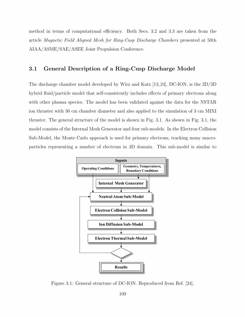
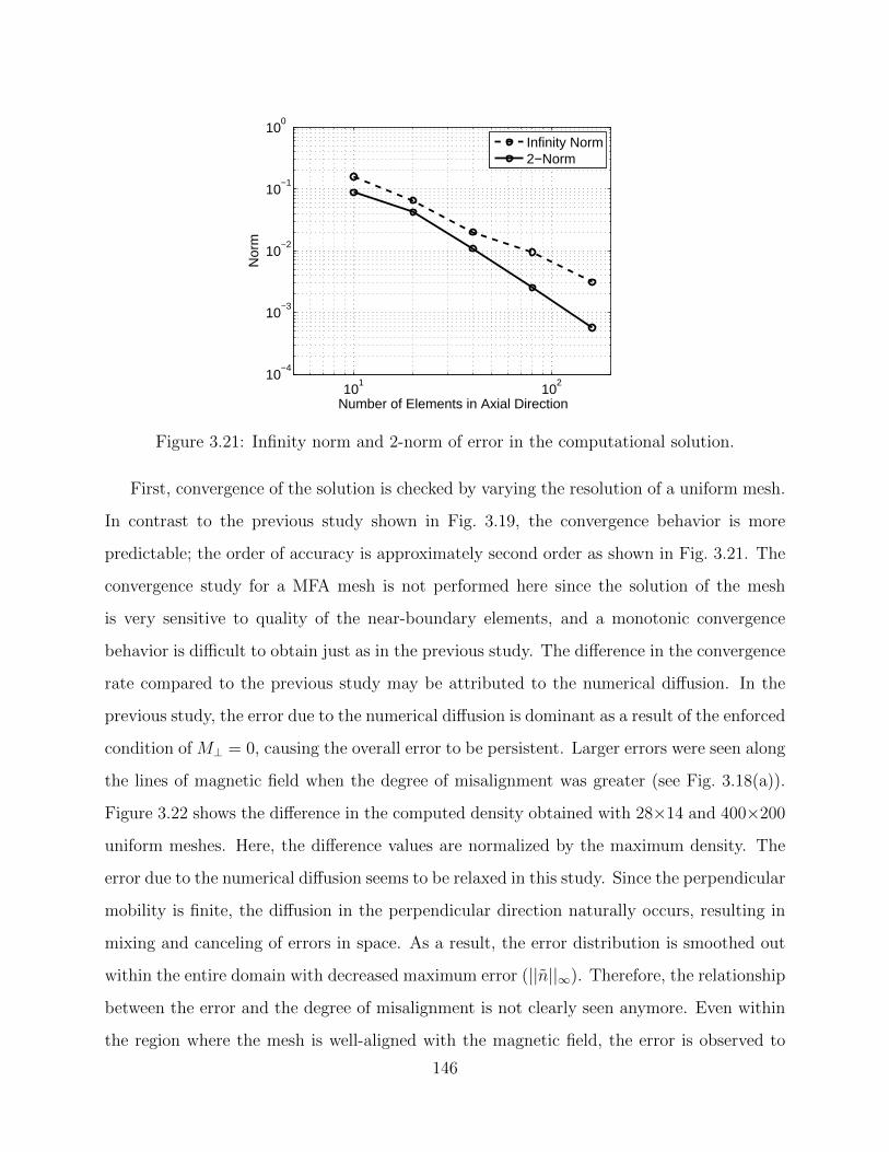
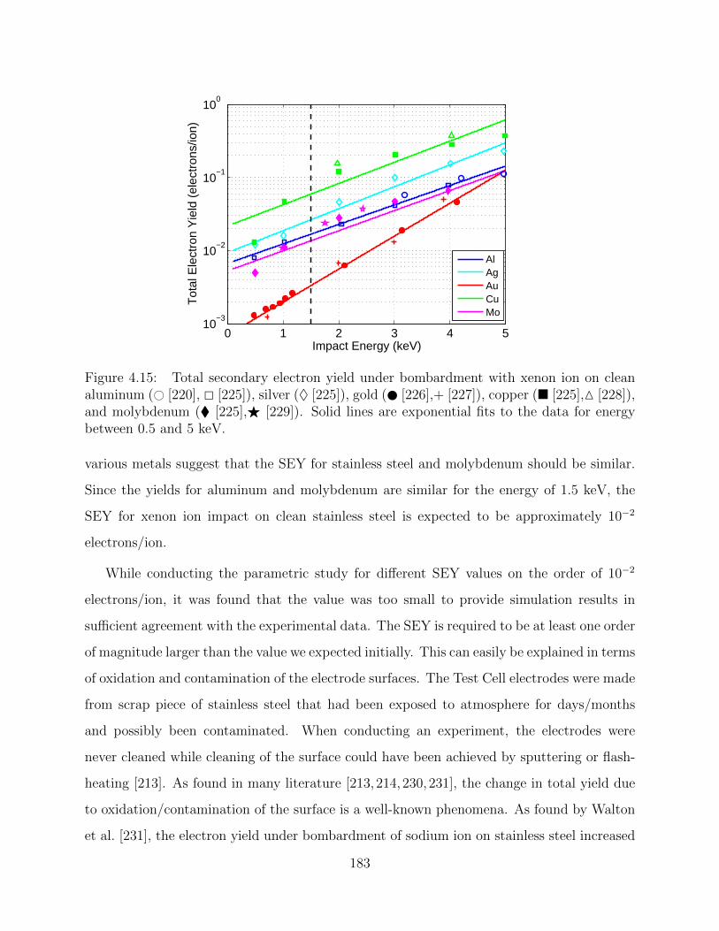
University of California Los Angeles Multi-Scale Multi-Species Modeling for Plasma Devices A dissertation submitted in partial satisfaction of the requirements for the degree Doctor of Philosophy in Aerospace Engineering by Samuel Jun Araki 2014
where s1 = c2d3 − c3d2, s2 = c2d4 − c4d2, and s3 = c4d3 − c3d4. The sum of the volumes
corresponds to the physical volume of the quadrilateral element. These formulas for corrected
volumes can be used for any grid with arbitrary quadrilaterals or triangles including uniform,
adaptive regular, non-orthogonal, and unstructured meshes in r-z cylindrical coordinates.
2.3.4.4 Implementation
For every node element, the weighted volumes are calculated using Eqs. (2.25) and (2.26) and
distributed to corresponding vertices (cell centroids). The sum of the volumes distributed
to one cell is the corrected volume used for the density calculations for the cell. Then, the
volumes assigned to the boundary cells are re-assigned to the nearest interior cells since
the volumes of the boundary cells are essentially zero. Therefore, the effective weighting
between the boundary cells and the neighboring interior cells are the nearest-grid-point
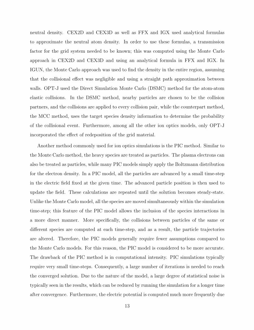
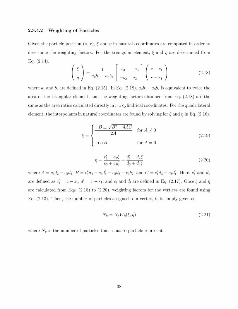
weighting as shown by the interpolation function in Fig. 2.4. At every time-step during
the tracking of particles, fraction of particles that a macro-particle represents is distributed
to three to four vertices of a node element in which the particle is located. The particles
weighted to the vertices are determined from Eqs. (2.13) and (2.18) to (2.21), depending
on the element shape, and these particles are accumulated at cell centroids until the end of
40
z
r10
3
4
5
6
2
0.0 1.0Wj(r)
Figure 2.4: Orthogonal mesh with variable spacing in radial direction. Closed and open dotsrepresent interior and boundary cells, respectively. Radial interpolation function, Wj(r), isshown to the right of the mesh.
the particle tracking. Again, the particles distributed to the boundary cells are re-assigned
to the nearest interior cells. Finally, the particle density at a cell is computed by dividing
the particles assigned to each cell centroid by the corrected cell volume. The Verboncoeur’s
approach allows a significant reduction in the computational cost since it does not require
complex weighting factor calculation that is performed at every particle position while the
weighted cell volumes are computed only once when the computational grid is generated.
2.3.5 Collisions
Atomic collision is a non-collective process that involves exchange of energy between the
same or different species. For most of the simulations, the background neutral density is
several orders of magnitude higher than the densities of other species. Therefore, we mainly
consider collisions of primary electrons, ions, and plasma electrons with background neutral
atoms. The collision process can be categorized by the types of energy exchange: elastic,
inelastic (excitation and ionization), superelastic, radiative and charge-reactive collisions [4].
The types of collisions included in the SC model are listed below.
• Electron-atom elastic collision
• Electron-atom ionization
• Electron-atom excitation
• Ion-atom elastic collision
41
The relative importance of different collision types can be determined by examining mean free
path, λ, for each collision type. The mean free path is related to collision cross-section, σ, and
density of target gas, n, by λ = 1/σn. Collision cross-section is an effective cross-sectional
area that a collision event may take place and is a measure of the collision probability.
The larger the cross-section and the density, the shorter the collision path length is, thus
collisions occur more frequently within the total path length that a particle travels. For
electron-atom collisions, elastic and inelastic collisions are considered to be important for
the simulation conditions because of the much larger cross-sections compared to those for
other collision types. For ion-atom collisions, only elastic (i.e. MEX) collision is included
in the SC model. Due to the low energy of ionized particles, inelastic collision is neglected
as ions only have energies below the threshold energy of the collision. The symmetric CEX
collision is also neglected because the resulting effect is similar to the MEX collision at the
ion and neutral energies. The primary electron-plasma electron collision is not implemented
in a direct manner but is incorporated by considering the equilibration (slowing) rate.
2.3.5.1 Elastic Collision
In an elastic collision, velocity vectors of the collision pair are altered while the total kinetic
energy is conserved, and no charge exchange occurs between the collision pair. After the
collision event, a charged particle initially gyrating about a magnetic field line is confined
by a different field line. The individual particles undergo a random walk as a result of
multiple elastic collisions, and the net effect is the diffusion of the particles across magnetic
fields. With a higher collision frequency, the diffusion across the fields is enhanced while the
diffusion along the fields is impeded.
The elastic collision is approximated using the Monte Carlo collision (MCC) method.
During a time-step, ∆t, the probability that a particle experiences an elastic collision is
expressed as
Pel = 1− exp(−∆tσelvno) (2.27)
where v is the velocity and no is the neutral density. Equation (2.27) gives a positive value
42
that is always less than or equal to 1. Whether an elastic collision event takes place is
determined by comparing Pel with a uniformly probable number between 0 and 1 generated
by the random number generator, U . The random number is updated for every instance it
appears in different equations. If Pel > U , then the particle experiences an elastic collision at
the given time-step. Once it is determined that the particle experiences an elastic collision,
we need to compute the post-collision velocity. The calculation of the velocity involves four
steps: (1) transformation of the pre-collision velocity to the center of mass (CM) frame,
(2) computation of the CM deflection angle, (3) determination of the CM post-collision
velocity, and (4) transformation of the post-collision back to the laboratory (LAB) frame.
The transformation between the two frames are provided in Appendix D.2.
Deflection Angle Calculation In applying the MCC method, it is necessary to obtain a
functional form of scattering angle χ as functions of the relative energy Er and the random
number U . This can be achieved by finding the differential cross-section, I = dσ/dΩ, and
then determining the probability that the particle is scattered at χ.
P (Er, χ) =
∫ χ0I(Er, χ
′)dχ′∫ 2π
0I(Er, χ′)dχ′
(2.28)
After solving the integrals in Eq. (2.28), the resulting equation can be manipulated to obtain
an expression for χ as functions of Er and P . In the MCC method, the probability, P , is
replaced by U in determining the scattering angles.
While the process of determining χ is relatively simple, it requires a knowledge of the dif-
ferential cross-section that can be applied for a range of relative energy values. Experimental
data for differential cross-section for elastic collisions between electrons and xenon atoms are
obtained by many authors [130–134], and these data agree fairly well with theoretical calcu-
lations [135,136] as shown in Fig. 2.5. Figure 2.5 also plots the differential cross-sections for
the scattering models [137,138] applied in many computational models. As seen in Fig. 2.5,
the pattern of the differential cross-section varies dramatically as incident energy changes.
For this reason, it is difficult to obtain a single curve-fit equation representing the differential
43
0 50 100 15010
−2
10−1
100
101
102
Scattering Angle (°)
dσ/d
Ω (
Å2 /s
r)
ModelTheoryExperiment
(a) 5 eV
0 50 100 15010
−1
100
101
102
Scattering Angle (°)
dσ/d
Ω (
Å2 /s
r)
ModelTheoryExperiment
(b) 10 eV
0 50 100 15010
−2
10−1
100
101
102
Scattering Angle (°)
dσ/d
Ω (
Å2 /s
r)
ModelTheoryExperiment
(c) 20 eV
0 50 100 15010
−3
10−2
10−1
100
101
102
Scattering Angle (°)
dσ/d
Ω (
Å2 /s
r)
ModelTheoryExperiment
(d) 50 eV
Figure 2.5: Differential cross-sections at different impact energies. Experimental measure-ments are shown by red markers (# [130], 2 [131], ♦ [132], M [133], + [134], and × [134]).Blue lines represent the theoretical results (solid [135] and dashed [136]). Black lines repre-sent the models often implemented in computational models (solid [137] and dashed [138]).
cross-section for the range of energy values. The theoretical calculations of the differential
cross-section may be implemented to accurately predict the scattering angles. However, it
would result in much longer computational run-time as the calculation has to be performed
for every incidence of elastic collision.
In the SC model, we use a simple formula derived by Okhrimovskyy et al. [137] for the
CM deflection angle calculation. This method is not perfectly accurate as shown in Fig. 2.5
but takes into account that the scattering is more forward-peaked with increasing energy.
44
More importantly, the determination of the deflection angle is very quick. Approximating
the electron-atom interaction potential by the screened Coulomb potential and using the
first Born approximation of quantum scattering, Okhrimovskyy et al. derived an expression
for the differential cross-section.
I(Er, χ) =1
4π
1 + 8ε
(1 + 4ε− 4ε cosχ)2(2.29)
where ε = Er/E0 is the dimensionless energy and E0 is the atomic unit of energy (E0 = 27.21
eV). Equation (2.29) is used in Eq. (2.28) to find the probability that an electron is scattered
at χ. Finally, a formula for the deflection angle can be derived by replacing P with U and
solving for χ.
cosχ = 1− 2U
1 + 8ε(1− U)(2.30)
For ion-atom elastic collision, the computational model employs the variable hard sphere
(VHS) molecular model [139]. Although the scattering characteristic of the model is not
completely realistic, the VHS model has been used in various simulations for rarefied gases
at relatively low energies and produced very accurate results. Also, the simple model allows
quick calculations of collision mechanics. In this model, the scattering is determined in the
same way as the hard sphere model, while the cross section is determined by the following
formula given by Dalgarno et al. [140] instead of using the physical cross section.
σi =64200
vrA
2(2.31)
The deflection angle is given as follows
χ = 2 cos−1√U (2.32)
Since the scattering is isotropic in the CM frame, the transformation between the CM and
LAB frames is not necessary; thus the method requires significantly less operations compared
to the other counterpart methods. The IB model described in Chapter 4 implements a more
detailed method, which was necessary due to the high energy of incident ions.
45
Inelastic Collision Inelastic collisions (i.e. ionization, excitation, etc.) between primary
electrons and background neutral atoms result in production of other species such as ions
and plasma electrons. In a single ionization event, the incident primary electron energy
is used to eject the bound electron of the atom. Since the threshold energy for a single
ionization collision is 12.13 eV, the primary electron loses an energy corresponding to the
threshold energy for every ionization event. Although the primary electron of 25 eV have
a sufficient energy to experience two ionization events, we assume for simplicity that the
primary electron join the plasma electron population after the event. Thus, every ionization
event results in one ion and two plasma electrons. In an excitation event, the kinetic energy of
the primary electron is transferred into some internal mode to create an atom in an excited
bound state. Similar to the ionization event, we assume that the primary electrons join
the plasma electron population after an excitation collision. The equilibration of primary
electrons interacting with the plasma electron population by Coulomb collisions is treated
similarly to the inelastic collisions. The equilibration rate is much faster after an inelastic
collision because of the reduced energy. If this equilibration rate is faster than the rate
of inelastic collision, then the assumption of primary electrons joining the plasma electron
population after a single inelastic collision would not be too far off from the reality.
In approximating inelastic collisions by the MCC method, a macro-particle current, J ,
is reduced at every time-step. A current of particles traveling for a given time-step, ∆t,
through a collection of species densities, n, is given as [141]
J(t+ ∆t) = J(t) exp(−∆t
∑(Kn)
)(2.33)
where K is the rate constant for different types of inelastic collisions. Effects of all the types
of inelastic collisions are included in∑
(Kn) such that
∑(Kn) = no (Kiz +Kex) + ns (Kslow) (2.34)
where subscripts iz, ex, and slow denote ionization, excitation, and equilibration processes,
respectively. The rate constants, Kiz and Kex, are simply calculated by K = vσ, and Kslow is
46
calculated using Spitzer particle-field slowing time as given in Appendix D.3. The percentage
of current lost due to all types of inelastic collisions is then expressed as
Pinel = 1− exp(−∆t
∑(Kn)
)(2.35)
The percentage of current lost due to each type of inelastic collision is obtained by the similar
equation.
Piz = 1− exp (−∆t(Kizno))
Pex = 1− exp (−∆t(Kexno)) (2.36)
Pslow = 1− exp (−∆t(Kslowns))
With these percentages of current lost, the reduction in the primary electron current by each
type of inelastic collision can be determined. The reduction in the primary electron current
at each time-step is computed by multiplying Pinel by the current before the time-step.
∆J = J(t)Pinel (2.37)
The current lost by each inelastic collision at each time-step is then given by
∆Jiz = ∆JPiz∑P, ∆Jex = ∆J
Pex∑P, ∆Jslow = ∆J
Pslow∑P
(2.38)
where∑P = Piz +Pex +Pslow is the sum of the percentages of the current lost. The amount
of representative current lost for each inelastic collision during the time step is added to the
local cell until the end of particle tracking. The total current loss due to the ionization event,∑(∆Jiz), is related to the ion generation rate density.
ni =
∑(∆Jiz)
eVcell
(2.39)
where Vcell is the volume of the cell in which the particle predominantly resides during the
47
time step. Similarly, the plasma electron generation density of the local cell is given by
ne =
∑(2∆Jiz + ∆Jex + ∆Jslow)
eVcell
(2.40)
These generation rate densities are used to determine the currents for macro-particles rep-
resenting numbers of ions and plasma electrons from the local cells.
2.3.5.2 Collision Cross-Sections
A collision cross-section is an effective area that a given type of collisional reaction occurs
and is directly related to a probability of the collisional event. By comparing cross-sections
for different reactions, relative importance of the specific collision type can be determined.
A collision cross-section depends on the types of particles involved and the relative energy
of the collision pair. Therefore, the data for the cross-sections as a function of energy have
to be gathered for every type of collision for the specific combination of the collision pair.
For electron-atom collisions, we consider three types of collisions: elastic, ionization, and
excitation collisions.
Numerous data for these collision cross-sections for the combination of electron and xenon
atom have been obtained by previous researchers. Among the cross-section data, we have
chosen the relatively recent experimental data as well as the data used the most commonly
in other computational models that are applicable for the energy range of interest. The
elastic collision cross-section data are obtained by Hayashi [142] and Register et al. [132].
The two data agree fairly well, while we choose to use the more recent data by Hayashi
to find the curve-fit equation for the type of collision. The ionization cross-section data
are obtained by Hayashi [142], Kobayashi et al. [147], Rejoub et al. [148], and Rapp and
Englander-Golden [149]. Although the data obtained by Rapp are the oldest among the
four data sets, we use Rapp’s data because the data set is the most commonly used in other
computational models. The excitation cross-section data are obtained by Hayashi [142,150],
Mason and Newell [151], de Heer et al. [152], Kaur et al. [153], and Ester and Kessler [154].
The excitation cross-section data are sparse in that none of the data sets agrees to each
48
10 20 30 40 50 60 700
10
20
30
40
50
Energy (eV)
Cro
ss−
Sec
tion
(Å2 )
TotalElasticInelastic
Figure 2.6: Cross-sections for total (# [142], + [143], 2 [144], × [145], and M [146]), elastic(# [142] and + [132]), and inelastic collisions. The solid lines represent the curve-fit equationsused in the SC model.
10 20 30 40 50 60 700
2
4
6
8
10
Energy (eV)
Cro
ss−
Sec
tion
(Å2 )
InelasticIonizationExcitation
Figure 2.7: Cross-sections for inelastic, ionization (# [147], + [148], 2 [142], and × [149]),and excitation (# [150], + [142], 2 [151], × [152], ♦ [153] and M [154]) collisions. The solidlines represent the curve-fit equations used in the SC model.
49
other. We use the data obtained by Hayashi [150] because the sum of cross-sections for all
the collision types agreed best with the total cross-section data for the energy of 25 eV when
using his excitation cross-section data.
The cross-section data and the curve-fit equations used in the model for different types
of collisions are shown in Figs. 2.6 and 2.7. These data sets for total, elastic, inelastic,
ionization, and excitation collision cross-sections are fitted with piecewise polynomials of
order 3 to 6. These fitting equations are formulated to cover the energy range of 0.1 to
1000 eV while a better fitting is obtained by using smaller segments for the range of energy
applicable to our simulation conditions.
2.3.6 Potential Solver
All the charged particles are tracked independently, yielding the charge density distribution
in the computational domain. This information is used to update the electric potential,
computed by applying the finite volume method to the integral form of Gauss’s equation.
∮E · dS =
y
V
ρfε0
dV (2.41)
where E is the electric field given as E = −∇φ, dS is the differential surface vector pointing
outward, ρf is the free charge density, and ε0 is the permittivity of free space. Equation (2.41)
is solved via control volume formulation for each cell.
∮cell
E · dS = −∮
cell
∇φ · dS =ρfVcell
ε0
(2.42)
The left hand side of Eq. (2.42) is evaluated along the cell edges. The standard way of
approximating ∇φ is to take a difference equation with the values at the cell of interest and
its neighboring cell as described in Sec. 2.3.6.1. For a uniform mesh, this method works
very well, and the solution is globally second order accurate. However, when applying the
simple method to an adaptive mesh, the accuracy drops locally across coarse/fine grid inter-
faces. Several researchers have addressed the problem and proposed a method performing
50
an interpolation to obtain a value inside a coarse cell and applying the difference equa-
tion [155–157]. The SC model uses a similar but more general method that can be used
even for non-uniform meshes. The method is introduced by Batishchev [158] and applied by
Fox [159] in his fully-kinetic PIC model. Details of the method are provided in Sec. 2.3.6.2.
2.3.6.1 First Order Potential Solver
In the first-order accurate method, the electric field across a cell face is approximated using
a finite difference equation. Consider the cells shown in Fig. 2.8 where the cell of interest and
the cell across the face, i, are denoted by s and n, respectively. Note that the cell vertices
are numbered to coincide with the cell face number so that the vertices of the cell face are
always i and i+ 1. The electric field across the cell face i is
Ei = −∇φ = − φn − φs√(zn − zs)2 + (rn − rs)2
isn (2.43)
where isn is the unit vector from cell center location of cell s to cell n expressed as,
isn =(zn − zs)z + (rn − rs)r√
(zn − zs)2 + (rn − rs)2(2.44)
(zs, rs)
(zn, rn)
(zi, ri)
(zi+1, ri+1)
fs
fn
Si
isn
Figure 2.8: Electric flux across the cell face i is determined with the nodal and cell-centeredcoordinates and cell-centered potential values.
51
Assuming that E = −∇φ is constant along the cell face, the flux across the cell face i
becomes ∫i
Ei · dS = Ei ·∫i
dS = Ei · Si (2.45)
where Si is the cell face vector pointing outward and is given as Si = π(ri+ri+1)(∆rz−∆zr).
Here, ∆r = ri+1 − ri, and ∆z = zi+1 − zi. Combining Eqs. (2.43) to (2.45), the flux across
the cell face is expressed as,
Ei · Si = Ciφs − Ciφn (2.46)
where
Ci = −π(ri + ri+1)(zn − zs)∆r − (rn − rs)∆z
(zn − zs)2 + (rn − rs)2(2.47)
Every cell has four to eight faces in an adaptive regular mesh, depending on refinement of
adjacent cells. Summing the fluxes across all the cell faces, Gauss’s law for each cell can be
expressed in terms of potentials at the cell of interest and the neighboring cells.
Nf∑i=1
Ei · Si =
Nf∑i=1
(Ciφs − Ciφni) =ρfVcell
ε0
(2.48)
where Nf is the number of cell faces. For a uniform mesh, this method is globally second
order accurate since the Laplacian in Poisson’s equation is a second derivative operator, and
the finite difference equation to the Laplacian is inherently second order accurate.
2.3.6.2 Second Order Potential Solver
Using the simple method described above, the accuracy drops to first order when the line
between two cell-centered locations and the cell face are not orthogonal. This situation arises
at coarse/fine grid interface of an adaptive mesh as well as in a non-uniform unstructured
mesh. Therefore, a more sophisticated method has to be implemented to retain the second-
order accuracy. The second-order method approximates the local variation in φ across a cell
face with the 2D quadratic equation [159].
φ = φs + a∆zs + b∆rs + c∆z2s + d∆zs∆rs + e∆r2
s (2.49)
52
where ∆zs = z−zs, ∆rs = r−rs, and a, b, c, d, and e are the coefficients to be solved. Since
Eq. (2.49) has five unknown coefficients, determining the coefficients require five independent
equations of φ; therefore, five different cell-centered points closest to the cell face are chosen
in addition to the current element. Let the neighboring cells be donated by 1 to 5, then the
linear system of equations can be packed into matrix and vector form.
Ax = f (2.50)
where
A =
∆zs1 ∆rs1 ∆z2
s1 ∆zs1rs1 ∆r2s1
......
......
...
∆zs5 ∆rs5 ∆z2s5 ∆zs5rs5 ∆r2
s5
, x =
a
b
c
d
e
, f =
∆φs1
...
∆φs5
and ∆φs = φ−φs. By finding inverse matrix of A, the coefficients can be expressed in terms
of potentials of the neighboring cells, x = A−1f .
Along a cell face, the line between the two cell nodes (i and i+1) is taken to be a straight
line. Thus, the relation between z and r is simply
r = αz + β z =r − βα
(2.51)
whereα =
ri+1 − rizi+1 − zi
β = ri − αzi (2.52)
With the quadratic approximation to φ given in Eq. (2.49), we can solve Eq. (2.42) for
each cell. The electric field E can be expressed in terms of the coefficients, the position of
the cell of interest, and the position along the cell face.
E = −∇φ = −(∂φ
∂zz +
∂φ
∂rr
)(2.53)
53
where∂φ
∂z= a+ 2c(z − zs) + d(r − rs)
∂φ
∂r= b+ d(z − zs) + 2e(r − rs)
Also, the differential area along the cell surface is given by dS = 2πr(drz − dzr). Unlike
the case described in Sec. 2.3.6.1, E across the cell face is not taken to be constant in this
method, so the integration along the cell face is done analytically.
∫E · dS = 2π
[∫−r∂φ
∂zdr +
∫r∂φ
∂rdz
]
= 2π
(−2
3aα− 1
3d+ 2
3eα
+ 13dα2
)(r3
2 − r31)
+(−1
2a+ c(β/α + zs) + 1
2drs)
(r22 − r2
1)
+(
12bα− e
αrs − 1
2dα
(β/α + zs))
(r22 − r2
1)
(2.54)
Finally, summing the fluxes across all the cell faces, Gauss’s law for each cell can be expressed
in terms of potentials at the cell of interest and the neighboring cells.
where ∆zsk = zk − zs and ∆rsk = rk − rs. Then, the square of the error over N neighboring
cells is,
R2 =N∑k
R2k =
N∑k
[φs + a∆zsk + b∆rsk + b∆z2
sk + d∆zsk∆rsk + e∆r2sk − φk
]2(2.67)
The error of the quadratic equation through all the cells is minimized when the partial
derivatives of Eq. (2.67) with respect to the coefficients are all zero.
∂R2
∂a= 0,
∂R2
∂b= 0,
∂R2
∂c= 0,
∂R2
∂d= 0,
∂R2
∂e= 0 (2.68)
The five equations from Eq. (2.68) can be expressed in matrix/vector form, and the coeffi-
cients can be computed by solving the linear system of equations.
Alternatively, the matrix from Eq. (2.68) can be directly derived from the overdetermined
linear system of equations. For N number of cells, the linear system of equations becomes
Ax = f (2.69)
where
A =
∆zs1 ∆rs1 ∆z2
s1 ∆zs1rs1 ∆r2s1
......
......
...
∆zsN ∆rsN ∆z2sN ∆zsNrsN ∆r2
sN
, x =
a
b
c
d
e
, f =
∆φs1
...
∆φsN
Here A is a 5-by-N matrix, and x is an array containing the coefficients for the 2D quadratic
equation, f is an array containing ∆φ = φs − φk where k = 1, ..., N . A unique solution for
the coefficients in an array x can be determined by multiplying both sides by the transpose
of matrix A from the left and finding the inverse of ATA.
x = [ATA]−1ATf (2.70)
Instead of applying Eq. (2.70) directly, the least squares problem is solved using the routine,
gels, available in Intel MKL.
60
Boundary Conditions for Electric Field The upstream, side wall, and downstream
plates of the cylindrical domain are either grounded or biased at fixed potential. Therefore,
the electric field along any electrode should always be zero. In addition, the radial component
of the electric field along the axis of symmetry is zero because of the symmetry. These
boundary conditions for the electric field is shown in Fig. 2.12. Although the potential is
input accordingly for the boundary cells, the boundary condition for the electric field is not
always satisfied by the least squares approach. In other words, the potential surface described
by the 2D quadratic equation does not necessarily go through the potential values at the
boundaries when the least squares method is used. In order to increase the accuracy near
the boundaries, the 2D quadratic equation is refined to ensure that the boundary conditions
are satisfied. Along the axis of symmetry, the expression for the radial component of the
electric field is given as
Er|r=0 = −b+ d(z − zs)− 2ers = 0 (2.71)
Since Eq. (2.71) has to be satisfied for any value of z along the axis, d has to be zero. Then,
Eq. (2.71) reduces to −b + 2ers = 0. Along the electrodes, similar approach can be used
to obtain additional constraints for the coefficients of the 2D quadratic equation. These
equations are summarized in Table 2.1.
z
r
0zE =
0rE = 0rE =
0rE =
Figure 2.12: Boundary conditions for electric field.
61
Table 2.1: Constraint equations for the 2D quadratic equation to enforce the boundaryconditions for electric field.
Boundary Constraints for Coefficients
Axis of symmetry, r = 0 d = 0, −b+ 2ers = 0
Upstream end, z = 0 e = 0, b− dzs = 0
Downstream end, z = zb e = 0, b+ d(zb − zs) = 0
Side wall of cylindrical domain, r = rb c = 0, a+ d(rb − rs) = 0
2.3.8 Mixing and Smoothing
Due to the structure of the SC model, charged species at thermal velocity (i.e. ions and
plasma electrons) overly respond to the small potential well resulted from a slight imbalance
of the positive and negative charges. For example, if there is a potential well that exceeds the
energy of ions, all the ions created near the region stays in the well while the plasma electrons
are quickly repelled from the region. This brings up the electric potential significantly higher
than a realistic value. In the next iteration, the potential peak then attracts the electrons
and repel the ions, again resulting in a large well. The alternation of the potential structure
continues, and the potential never converges to a final solution. In order to mitigate this
effect, the SC model mixes the computed species densities for the current iteration with
the values in the previous iterations. Let the subscripts in and out denote the species
densities used to compute the electric potential and obtained directly after the particle
tracking routines at iteration k, respectively. The species density used to compute the
potential for the next iteration is determined by
nk+1in = (1− ξ)
k∑j=k−Nk
njin + ξk∑
j=k−Nk
njout (2.72)
where ξ is the mixing factor and Nk is the number of previous iterations to mix. Also,
the change in the density from the previous iteration is limited to be within an order of
magnitude such that nkout = min(nk∗out, 10 nk−1in ) where the superscript ∗ denotes the raw
output value from the particle tracking.
62
The mixing technique smooths the behavior of the solution in the iteration space. On
the other hand, the smoothing technique reduces the statistical fluctuations in the physical
space at each iteration. Smoothing is done by mixing the charge densities of nearby cells
while keeping the total number of particles the same. Since the cell volumes are constant in
the axial direction in a uniform mesh, a simple binomial filter function can be applied.
ρk+10 =
3
4ρk0 +
1
4ρk1
ρk+1i =
1
4ρki−1 +
1
2ρki +
1
4ρki+1, 0 < i < Nz (2.73)
ρk+1Nz
=1
4ρkNz−1 +
3
4ρkNz
where ρ is the charge density, i is the cell index in the axial direction, and Nz is the number
of cells along the z-axis. Note that Eq. (2.73) is the smoothing for the cell-centered quantity
so that the smoothing for the node-centered quantities is slightly different. In the radial
direction, the coefficients need to be derived by considering the variation in cell volume [160].
ρk+10 = (1− α0)ρk0 + α0ρ
k1
ρk+1j = αjρ
kj−1 + (1− 2αj)ρ
kj + αjρ
kj+1, 0 < j < Nr (2.74)
ρk+1Nr
= αNrρkNr−1 + (1− αNr)ρkNr
where
α0 =1
4, α1 =
α0V0
V1
, αj =2αj−1Vj−1
Vj− αj−2Vj−2
Vj, αNr =
αNr−1VNr−1
VNr(2.75)
Here, i is the cell index in the radial direction and Nr is the number of cells along the radius.
For the node-centered quantities, α0 is replaced with 12. Therefore, for an interior cell, the
charge density is mixed with values at the cell of interest and eight surrounding cells with
coefficients as in Eq. (2.76)
αj
1− 2αj
αj
[
1
4
1
2
1
4
]=
14αj
12αj
14αj
14(1− 2αj)
12(1− 2αj)
14(1− 2αj)
14αj
12αj
14αj
(2.76)
63
Packing all the coefficients and charge densities for all the cells in the vector-matrix form,
a single pass smoothing is done by applying P 1 = AP 0 where P is the array containing all
the ρs and A is the matrix containing the coefficients for all the cells. This can be extended
for multiple passes by
P k = AMP 0 (2.77)
where M is the number of passes. AM can be precomputed before the main program. While
the technique reduces the number of completely unrealistic trajectories of charged species
due to the unphysical potential wells and peaks, it may mask the important characteristic
in the plasma structure. Therefore, the degree of mixing is reduced by decreasing M as
reaching the final solution.
2.3.9 Convergence
Convergence of the solution is determined by the change in the electric potential and species
densities between the iterations. Two different vector norms are used for the convergence
criteria: the 2-norm and the maximum norm. The 2-norm provides information on how
much the potential structure has changed from the previous iteration.
||δφ||2 =
√√√√ N∑i
(φk+1i − φki )φk+1i
(2.78)
where i denotes the cell number, N is the number of cells, and k is the iteration step. On
the other hand, the maximum norm tells the percentage change in the maximum potential
value.
||δφ||∞ = maxi
(φk+1
i − φki )φk+1i
(2.79)
Similar norms can be obtained for species densities. When these norms are smaller than
some tolerance, ε, specified as an input, then the solution is considered to be converged.
64
2.4 Component Level Validations
2.4.1 Particle Weighting in Cylindrical Coordinates
2.4.1.1 Numerical Assessment of Density Errors
Density errors arising from the cell-centered weighting algorithm are computed for different
radial density profiles in an adaptive regular mesh and a unstructured mesh as shown in
Fig. 2.13. The adaptive regular grid allows for testing of mixed quadrilateral and triangle
node elements at the coarse/fine grid interface. The unstructured mesh contains quadrilat-
eral node elements that are shaped differently throughout the test domain. Three different
radial density profiles are used to investigate their effects to the density errors: 1) uniform,
2) linearly decreasing, and 3) Bessel function. For the case of a uniform density, the com-
puted density profile should be exact if the corrected volume formulas are applied properly.
The Bessel function profile is chosen since this can physically arise in glow discharges; the
solution can be obtained by solving the diffusion equation (−D⊥∇2n = βn) in cylindrical
coordinates [161]. The functional form of the exact density profiles are given in Table 2.2. In
the test program, radial positions of the macro-particles are determined by finding the radius
that satisfy the equations provided in Table 2.2 for a given random number, U , between 0
and 1. Then, macro-particles are advanced in a direction perpendicular to the downstream
end. At every time-step, fraction of particles that a macro-particle represents is distributed
to three to four vertices of a node element in which the particle is located. The particles
weighted to the vertices are determined from Eqs. (2.13) and (2.18) to (2.21), depending on
the element shape, and these particles are accumulated at cell centroids until the end of the
particle tracking. Again, the particles distributed to the boundary cells are re-assigned to
the nearest interior cells. Finally, the particle density at a cell is computed by dividing the
particles assigned to each cell centroid by the corrected cell volume. For all the test cases,
computational results are obtained with 1, 000, 000 macro-particles and 2, 000 time-steps
before reaching the downstream end.
65
z
r
(a) Adaptive regular mesh
z
r
(b) Unstructured mesh
Figure 2.13: Two meshes used in the numerical test for particle weighting algorithm. Thesolid line corresponds to cell boundaries, and the dashed line corresponds to node elementboundaries.
Table 2.2: Equations for exact solution and particle injection position for different densityprofiles examined. Here, n0 is the centerline density, R is the normalized radius (R = r/rmax),U is the random number between 0 and 1, J0 is the zeroth-order Bessel function of the firstkind, and k1 is the first root of J0.
Density profile Exact solution Particle injection
Uniform n(R) = n0 U = R2
Linear n(R) = n0(1−R) U = 3R2 − 2R3
Bessel n(R) = n0J0(k1R) U = RJ1(k1R)/J1(k1)
66
Adaptive regular mesh Figures 2.14 to 2.16 show the relative error for uniform, linearly
decreasing, and Bessel function density profiles, respectively, when using the standard area
weighting and the generalized weighting scheme in an adaptive regular mesh. In Fig. 2.14(a),
the errors at top and bottom cells apart from the grid interface are 9.3×10⁻³ and 8.3×10⁻²,
respectively. These errors are consistent with the results provided in Ref. [129] for one dimen-
sional radial grid; the errors can be derived analytically by using nearest-grid-point weighting
between boundary cells and the neighboring interior cells. At the grid interface, the error
becomes more severe, reaching a value of 0.47. As shown in Fig. 2.14(b) for the case of
uniform density profile, all of these systematic errors are removed by using the generalized
weighting scheme. The systematic errors at the top and bottom cells are eliminated com-
pletely, and the densities at cells along the grid interface almost perfectly match the expected
values with errors of less than 3.3×10⁻⁶, thus showing that the cell-centered weighting algo-
rithm has been implemented properly. Using the standard area weighting for the cases with
non-uniform density profiles (Figs. 2.15(a) and 2.16(a)), the errors along the grid interface
are still dominant. These errors are reduced significantly when the generalized weighting
scheme is used (Figs. 2.15(b) and 2.16(b)). Although the errors in outermost interior cells
have slightly increased, it is insignificant compared to the reduction in errors at the grid in-
terface. Furthermore, Figs. 2.15(b) and 2.16(b) clearly show the reduction in density errors
in the region of a finer grid size; thus, the benefit of using the adaptive regular mesh can be
realized.
Unstructured mesh Figures 2.17 to 2.19 show the relative error for uniform, linearly
decreasing, and Bessel function density profiles, respectively, when using the two weighting
algorithm in a non-uniform mesh. As shown in Fig. 2.17, density errors are, again, reduced
drastically when using the generalized weighting scheme, and the density profile is almost ex-
actly uniform. For all the density profiles with the standard weighting scheme (Figs. 2.17(a),
2.18(a) and 2.19(a)), the distribution of the density error is comparable. The errors are
generally smaller away from the boundary, and very large errors are seen in the triangular
cells and quadrilateral cells with large aspect ratio that touch the boundaries. The maxi-
67
mum density errors are 1.4, 3.9, and 4.0 for uniform, linearly decreasing, and Bessel function
density profiles, respectively. One of the primary reasons for the large errors are the poor
smoothness of the grid; the change in cell size is very large from those cells to the neighboring
cells. When connecting the cell centroids, the midpoint of the line does not lie sufficiently
close to the cell edge. This indicates that the effective cell shape is significantly different
from the actual shape for those cells near boundaries. The large errors at those cells can
be alleviated by using a mesh that covers, in addition to the domain, a region outside the
domain. In this way, the cell centroid locations are not affected by the domain boundaries.
To apply the generalized weighting scheme, the limits in the corrected volume calculation,
Eq. (2.24), have to be modified to exclude the region outside the domain. The modifications
to the boundary treatment have not implemented herein since it is beyond the scope of this
paper. Another primary reason for the large errors is the non-uniform profile of density, as
indicated by increased errors at cells touching the boundary with R = 1 (or r = rmax). When
using the area weighting, the region where the particle is distributed to a cell centroid is
larger than the actual cell area. If the density value is greater at a neighboring cell, a larger
number of particles are weighted to the cell of interest. This is the main reason that density
errors at the cells touching the boundary with R = 1 persist even when using the generalized
weighting scheme, while the errors at all the cells near both ends are corrected and become
comparable to the neighboring cells (Figs. 2.18(b) and 2.19(b)). Note that the density profile
is uniform in axial direction for all cases. A further discussion for the density errors near
the boundary at R = 1 are provided in Sec. 2.4.1.2. In spite of the relatively larger density
errors, the maximum errors for generalized weighting scheme are reduced significantly, by
more than 50%.
2.4.1.2 Effect of Near-Boundary Density Error in Potential Solution
A further analysis for the Bessel function density profile has been conducted in order to
examine the effect of the grid size and the relatively large errors near the boundary to electric
potential solution. In this analysis, the electric potential is computed on a uniform radial
grid with number of interior cells of N = 5, 10, 20, and 40. Given the density profile provided
68
z
r
0.40
0.30
0.20
0.10
0.05
0.04
0.03
0.02
0.01
(a) Standard weighting scheme
z
r
3.5E-06
3.0E-06
2.5E-06
2.0E-06
1.5E-06
1.0E-06
5.0E-07
(b) Generalized weighting scheme
Figure 2.14: Relative error in density computed for uniform density profile in an adaptiveregular mesh.
z
r
0.40
0.30
0.20
0.10
0.05
0.04
0.03
0.02
0.01
(a) Standard weighting scheme
z
r
0.40
0.30
0.20
0.10
0.05
0.04
0.03
0.02
0.01
(b) Generalized weighting scheme
Figure 2.15: Relative error in density computed for linearly decreasing density profile in anadaptive regular mesh.
z
r
0.40
0.30
0.20
0.10
0.05
0.04
0.03
0.02
0.01
(a) Standard weighting scheme
z
r
0.40
0.30
0.20
0.10
0.05
0.04
0.03
0.02
0.01
(b) Generalized weighting scheme
Figure 2.16: Relative error in density computed for Bessel function density profile in anadaptive regular mesh.
69
z
r
1.00
0.90
0.80
0.70
0.60
0.50
0.40
0.30
0.20
0.10
0.05
0.02
0.00
(a) Standard weighting scheme
z
r
3.0E-06
2.0E-06
1.0E-06
5.0E-07
1.0E-07
1.0E-08
(b) Generalized weighting scheme
Figure 2.17: Relative error in density computed for uniform density profile in a non-uniformmesh.
z
r
3.00
2.00
1.00
0.80
0.60
0.40
0.20
0.10
0.05
0.02
0.00
(a) Standard weighting scheme
z
r
3.00
2.00
1.00
0.80
0.60
0.40
0.20
0.10
0.05
0.02
0.00
(b) Generalized weighting scheme
Figure 2.18: Relative error in density computed for linearly decreasing density profile in anon-uniform mesh.
z
r
3.00
2.00
1.00
0.80
0.60
0.40
0.20
0.10
0.05
0.02
0.00
(a) Standard weighting scheme
z
r
3.00
2.00
1.00
0.80
0.60
0.40
0.20
0.10
0.05
0.02
0.00
(b) Generalized weighting scheme
Figure 2.19: Relative error in density computed for Bessel function density profile in anon-uniform mesh.
70
in Table 2.2, the exact solution for potential can be solved analytically.
φ(R) = φ0J0(k1R) (2.80)
where φ0 is the potential at the centerline. Note that both Eq. (2.80) and the density profile
given in Table 2.2 are simply a function of the zeroth-order Bessel function of the first kind
and that the normalized profiles are identical. Macro-particles distributed properly along
the radius are weighted to cell centroids using the same weighting algorithm described in
Sec. 2.3.4; the particles are distributed to the cell-centroids, then the particles distributed to
the boundary cells are re-assigned to the nearest interior cells. Once the particle densities at
the cells are determined, the finite volume method is used to compute the potential at the
cells. Neumann (∂φ∂r
= 0) and Dirichlet (φ = 0) boundary conditions are applied at R = 0
and R = 1, respectively. Finally, the computed electric potential is compared with the exact
solution.
Figure 2.20 shows the normalized density profile obtained from the analytical solution
given in Table 2.2 and computed for four different mesh sizes. Although it is difficult to see
the degree of accuracy, it is readily seen that the computed density agrees, to the first order,
with the exact solution for all the meshes. Figure 2.21 plots the relative error along the radial
grid. Note that the relative error for the case of N = 5 is consistent with the coarse mesh
region in Fig. 2.16(b). For all the meshes, the error is the minimum for the innermost cell.
This is expected since the density profile is closest to uniform, and the corrected volume is
derived for the uniform density profile. With the increasing radius, the error monotonically
increases, reaching the maximum error at the outermost cell. The density error away from
the boundary at R = 1 is proportional to the square of the cell size (the second order
accuracy), while the maximum error value located at the outermost appears to increase with
finer mesh, as shown in Figs. 2.21 and 2.23. The increasing error with radius can be explained
by the monotonically decreasing density profile. For the density profile, the area weighting
results in a larger number of particles to be weighted to cell centroids from location below
when compared to nearest-grid-point weighting, and less particles from location above. For
71
interior cells, particle distribution from below and above the cell centroid can cancel out
to some degree. For the outermost cell, the number of weighted particles is always greater
when compared to the nearest-grid-point weighting. Furthermore, since the density is the
minimum at the outermost cell, the relative error is sensitive to the inaccuracy of weighting,
causing an apparent inflation of the error by orders of magnitude. Although the density
errors at outermost cells persist with smaller grid size, the potential solution converges with
grid size and is the second order accurate, as shown in Figs. 2.22 and 2.23. At the outermost
cell, the relative error is large; however, the magnitude of the density is small, so the density
in the cell has only a small effect to the solution in electric potential.
0 0.2 0.4 0.6 0.8 10
0.2
0.4
0.6
0.8
1
Density
Rad
ial P
ositi
on
N=5N=10N=20N=40Exact Solution
Figure 2.20: Normalized density profile
10−4
10−3
10−2
10−1
100
0
0.2
0.4
0.6
0.8
1
Relative Error
Rad
ial P
ositi
on
N=5N=10N=20N=40
Figure 2.21: Relative error in density
10−4
10−3
10−2
10−1
100
0
0.2
0.4
0.6
0.8
1
Relative Error
Rad
ial P
ositi
on
N=5N=10N=20N=40
Figure 2.22: Relative error in potential solu-tion
101
102
10−4
10−3
10−2
10−1
100
Number of Interior Cells
Infin
ity N
orm
DensityPotential
Figure 2.23: Infinity norm for density andpotential solutions
72
2.4.2 Potential Calculation
A numerical test on the potential solver described in Sec. 2.3.6.2 has been performed to
check the implementation and to show the second-order accuracy. The standard method
described in Sec. 2.3.6.1 is also implemented for comparison. In this test, electric potential
is calculated on a cylindrical domain with the end wall biased at 100 V and the other
walls grounded (0 V). The solutions computed with the two methods are compared with an
analytical solution obtained by solving the Laplace equation in cylindrical coordinates.
∇2φ(r, θ, z) =1
r
∂φ
∂r+∂2φ
∂r2+
1
r2
∂φ
∂θ+∂2φ
∂z2= 0 (2.81)
The general solutions for the Laplace equation is obtained by applying separation of vari-
where A, B, C, D, E, and F are some constants, Jm and Ym are the mth order Bessel
function of first and second kind, Im and Km are the mth order modified Bessel function of
first and second kind, kn is constant, and m and n are integers. In this specific problem,
we use Eq. (2.82) to find the analytical solution. In Eq. (2.82), m has to be 0 to satisfy
axisymmetric condition, and a few terms can be eliminated based on the boundary conditons.
Then, Eq. (2.82) is simplified as
φ(r, z) =∞∑n=1
Gn sinh(knz)J0(knr) (2.84)
where Gn are constants, kn is determined by setting J0(kna) = 0 which corresponds to
kna=2.4048, 5.5201, 8.6537, · · · , and a is the radius of the domain. Gn can be determined
73
Figure 2.24: Contour plot of potential (V) calculated with the analytical solution for thecase with a cylindrical domain with end plate biased at 100 V. The solutions are comparedfor the cells inside the dashed box.
using orthogonal property of J0 and sinh functions.
Gn =2V0
knaJ1(kna) sinh(knL)(2.85)
The analytical solution given in Eq. (2.84) involves infinite sum of sinh J0. For this numer-
ical test, 1000 terms are added; the number of terms is determined so that the solution is
computed reasonably accurately within an acceptable amount of time. A plot of potential
contour for the test problem is shown in Fig. 2.24. Even with the number of terms used to
compute the solution, the lower accuracy at the circumference of the end plate is inevitable
because of the sudden change of the boundary condition from the end plate to the cylinder
wall. Therefore, the solutions are only compared within the dashed box shown in Fig. 2.24.
Figures 2.25 and 2.26 show the relative errors for the solutions computed by the first-
order and the second-order methods in a non-uniform mesh. The first-order method produces
relatively larger errors at the cells near the coarse/fine grid interface when compared to errors
in the uniform region. This is expected since the method becomes second order in a uniform
mesh. These errors at the grid interface are removed when using the second-order method
as seen in Fig. 2.26. Figure 2.27 shows the change in the maximum relative error for three
different grid resolutions. By finding the slope of the lines, the order of convergence can be
74
determined. As seen in Fig. 2.27, the standard method provides a second-order accurate
solution when using a uniform mesh. However, the order of accuracy drops by one order for
an adaptive mesh. The accuracy is recovered when using the spline method for the same
mesh.
z (cm)
r(cm)
0 1 2 3 4 5 6 70
1
2
3
2.8E -02
2.6E -02
2.4E -02
2.2E -02
2.0E -02
1.8E -02
1.6E -02
1.4E -02
1.2E -02
1.0E -02
8.0E -03
6.0E -03
4.0E -03
2.0E -03
1.0E -03
Figure 2.25: Plot of relative error in electric field solution using the first order method.
z (cm)
r(cm)
0 1 2 3 4 5 6 70
1
2
3
2.8E -02
2.6E -02
2.4E -02
2.2E -02
2.0E -02
1.8E -02
1.6E -02
1.4E -02
1.2E -02
1.0E -02
8.0E -03
6.0E -03
4.0E -03
2.0E -03
1.0E -03
Figure 2.26: Plot of relative error in electric field solution using the least squares approach.
Figure 2.27: Convergence of potential solutions computed with the first- and second-ordermethods in an adaptive regular mesh.
2.4.3 Electric Field Calculation
The same test condition studied in Sec. 2.4.2 is used for the numerical test of electric field
calculation. The analytical solution for the electric field can be computed by simply taking
the gradient of φ given in Eq. (2.84).
Er(r, θ, z) =∞∑n=1
knGn sinh(knz)J1(knr) (2.86)
Ez(r, θ, z) = −∞∑n=1
knGn cosh(knz)J0(knr) (2.87)
where J1 is the first order Bessel function of the first kind. In this test, the potential obtained
from Eq. (2.84) is used to compute the electric field with Fox’s first-order method [159]
described in Sec. 2.3.7.1 and the least squares (second-order) method described in Sec. 2.3.7.2.
Similar to the test result for potential described in Sec. 2.4.2, the errors from the first-
order method are greater at the coarse/fine grid interface compared to uniform grid region as
shown in Fig. 2.28. These errors are removed when using the least squares approach as shown
76
in Fig. 2.29. Figure 2.30 shows the convergence of the electric field solutions. By comparing
the slope, it is clearly seen that the difference in the order of accuracy obtained from Fox’s
method and least squares method in an adaptive mesh. Although the Fox’s method provides
the second-order accurate solution in a uniform mesh, the order of accuracy drops to first-
order when using the adaptive mesh, and the accuracy is recovered to second-order when
using the least squares method. Furthermore, examining Fig. 2.28, less errors are found in
the region of finer grid, thus the benefit of the adaptive mesh has been demonstrated.
z (cm)
r(cm)
0 1 2 3 4 5 6 70
1
2
3
1.0E -02
9.0E -03
8.0E -03
7.0E -03
6.0E -03
5.0E -03
4.0E -03
3.0E -03
2.0E -03
1.0E -03
5.0E -04
1.0E -04
Figure 2.28: Plot of relative error in potential solution using the standard method.
z (cm)
r(cm)
0 1 2 3 4 5 6 70
1
2
3
1.0E -02
9.0E -03
8.0E -03
7.0E -03
6.0E -03
5.0E -03
4.0E -03
3.0E -03
2.0E -03
1.0E -03
5.0E -04
1.0E -04
Figure 2.29: Plot of relative error in potential solution using the spline method.
77
101
102
10−3
10−2
10−1
Number of parent cells in z−direction
Max
imum
rel
ativ
e er
ror
Least Squares Method (Adaptive Mesh)First Order Method (Adaptive Mesh)First Order Method (Uniform Mesh)
Figure 2.30: Convergence of electric field solutions computed with Fox’s method and theleast squares approach in an adaptive regular mesh.
2.5 Simulation Results
The SC model is used to simulate a variety of plasmas with increasing complexity of the
system. The simulation starts from an electron plasma that contains only the primary
electrons in a magnetic field created by a single cylindrical permanent magnet (Sec. 2.5.1).
An electron flood gun is used as the source of the nearly mono-energetic primary electrons.
This simulation is mainly to validate important components of the computational model,
most critically the electron tracker and magnetic field calculations. Then, the neutral gas
is introduced in the system, yielding a sparse plasma with four different species: primary
electrons, ions, plasma electrons, and neutral atoms (Sec. 2.5.2). Here, the sparse plasma
refers to a plasma with very low density such that the Debye length is comparable to the
plasma volume. Multiple block magnets are used in addition to the cylindrical magnet
to increase the primary electron confinement. In the ring-cusp configuration, the sparse
plasma as a whole is simulated to study the loss behavior of plasma species (Sec. 2.5.2.1).
Then, the confinement is improved by adding another ring-cusp; a close-up study of the
primary electrons was necessary to obtain a comparable result with the experiment. While
78
the electron gun was used in the simulations for the primary electron confinement and the
sparse plasma due to its well-known gun characteristic, the gun was later replaced with
a hollow cathode to achieve a higher ionization rate and a plasma condition that is more
applicable to ion thrusters (Sec. 2.5.3).
2.5.1 Primary Electron Confinement
The simulation using the SC model starts from an examination of the 25 eV primary electron
structure near the cusp in the absence of other species, mainly to validate important compo-
nents of the computational model. As shown in the primary electron trajectories (black lines
in Fig. 2.31), the primary electrons are ejected from the left along the axis of the discharge
domain, toward the cylindrical magnet placed downstream, at a divergence angle of 10–15
and a beam radius of 0.5 mm. Initially, the electrons are effectively not magnetized, and their
trajectories are approximately straight until the magnetic field strength becomes sufficiently
strong. Then, the electrons start to gyrate about the field lines and their gyroradii become
smaller as the magnetic field becomes stronger toward the magnet, with increasing likelihood
of magnet mirroring as they approach the cusp. Figure 2.32 compares the wire scan results
obtained from the experiment [163] and the computational model at the locations shown
in Fig. 2.31. These results show a good quantitative and qualitative agreement, indicating
that the particle tracking technique and the magnetic field calculations are fairly accurate.
One of the causes of the slight disagreement is likely the misalignment of the magnet and
electron gun axes during the experiment, as seen in the asymmetric scan profile obtained
during the experiment. Another reason for the disagreement is that the distance from the
magnet can only be obtained within certain accuracy in the experiment, and the uncertainty
is comparable with the step-size of position for the wire scan.
79
z ( cm)
r ( c
m)
0 100
10
20
30
0.04|B | (G) : 5 10 15 20 25 30 35 40 45 50 55
20 30 40 50 60 70
r (c
m)
60 62 64 66 68 70 72
2
4
6
8
10
(a)(b)(c)(d)
z (cm)
Figure 2.31: Primary electron trajectories (black lines) in 2D. The white lines represent themagnetic field lines. The dash-dot lines represent the wire scan locations.
−0.3 −0.2 −0.1 0 0.1 0.2 0.30
100
200
300
400
500
600
700
800
900
x (cm)
Wire
Cur
rent
(nA
)
SimulationExperiment
(a) 1.05 cm
−0.3 −0.2 −0.1 0 0.1 0.2 0.30
100
200
300
400
500
600
700
800
900
x (cm)
Wire
Cur
rent
(nA
)
SimulationExperiment
(b) 0.95 cm
−0.3 −0.2 −0.1 0 0.1 0.2 0.30
100
200
300
400
500
600
700
800
900
x (cm)
Wire
Cur
rent
(nA
)
SimulationExperiment
(c) 0.85 cm
−0.3 −0.2 −0.1 0 0.1 0.2 0.30
100
200
300
400
500
600
700
800
900
x (cm)
Wire
Cur
rent
(nA
)
SimulationExperiment
(d) 0.75 cm
Figure 2.32: Comparison of wire scan results from the simulation and the experiment. Thedistances from the magnet surface to the wire scan locations are given in the sub-figurecaptions.
80
2.5.2 Sparse Plasma
2.5.2.1 Structure and Leak Mechanism of Sparse Plasma
The confinement of the primary electrons is not sufficient to cause enough ionization by
simply introducing a neutral gas in the single cusp configuration. In addition, the other
plasma species such as ions and plasma electrons are lost to the walls too quickly and are
not maintained in the domain. For this reason, multiple block magnets are placed around the
circumference of the test cell and the electron gun to increase the confinement. A schematic of
the experiment simulated by the SC model is shown in Fig. 2.33. The detailed description of
the experimental apparatus is provided in Ref. [163]. The plasma is obtained by shooting the
25 eV primary electron beam of 50 µA into the test cell at the base pressure of 5×10⁻⁸ Torr
and at the xenon gas pressure of 1× 10⁻³ Torr. The electron gun is placed upstream of the
test cell in order to account for its limit in the neutral pressure. The dimension of the test cell
is 4 cm in length and 1.78 cm in radius. Since the mean free path of the ionization collision
is . 1.0 m, the primary electrons need to experience a number of reflection at magnetic
cusps before ionizing the neutral atom. While the other plasma species are generated by
Figure 2.33: Schematic of the discharge experiment for a sparse plasma. The contour plotof magnetic field strength (Gauss) is shown inside the test cell. The white lines representmagnetic field lines. The SC model is used to simulate the same domain.
81
the inelastic collisions, the achievable plasma density remains low due to the low primary
electron current. The electron density is on the order of 1012to1014 m−3. Here, we call our
plasma a sparse plasma, in which the Debye length is comparable to the plasma volume such
that the plasma is not quasi-neutral.
Figures 2.34 and 2.35 show the experimental results for the current densities in front
of the cylindrical magnet at the base pressure and at the pressure of 1 × 10⁻³ Torr. The
white “×” and dotted circle indicate the center and edge of the cylindrical magnet face,
respectively. It is readily noticeable that the current densities are not peaked at the center
of the magnet. This is due to the difficulty in perfectly aligning the electron gun with the
magnet center. At the scale of the species loss, even 1 mm of the misalignment can have a
significant impact on the loss pattern. At the base pressure, distinct ridges are present in
the results, whereas the ridges are slightly smoothed out when introducing the xenon gas.
On the other hand, the ion current density contour does not exhibit the ridge structure. The
cause of these loss patterns will be explored in Sec. 2.5.2.2.
A simulation of the experiment is carried out by the SC model. In this simulation, it is
assumed that 300 K xenon atoms are filled uniformly within the domain. The plasma electron
temperature is assumed to be 3 eV. Figure 2.36 shows the electric potential computed by
the SC model. All the electrodes are grounded, so the Dirichlet boundary condition of
φ = 0 are applied in the simulation. The highest potential value is seen close to the center
of the cylindrical domain while the potential drops rapidly towards the boundaries. This
potential structure pushes ions toward the walls. Figure 2.37 shows the contour plot of
primary electrons. The density is relatively higher at the single magnetic cusp. By design,
the stronger magnetic field strength at the ring-cusps reflect the electrons, while a larger
number of electrons reach the downstream electrode because of the relatively weaker field at
that surface. The contours for ion and plasma electron generation rate density are similar
to the primary density contour; thus, the vast majority of ions and plasma electrons are
created very near the cusp for plasma condition created by the electron gun. The ion and
plasma electron density contours are shown in Figs. 2.38 and 2.39. While the ion density is
peaked near the magnetic cusp, the plasma electron density is higher in the two regions of
82
Figure 2.34: Contour plot of the electron current density measured during the experimentat base pressure of 5× 10⁻⁸ Torr.
(a) Electrons (b) Ions
Figure 2.35: Contour plot of the current densities measured during the experiment at pressureof 1× 10⁻³ Torr.
z (cm)
r (c
m)
10
0.5
1.0
1.5
15
14
13
12
11
10
9
8
7
6
5
4
3
2
12 3 40
Figure 2.36: Electric potential (V) calculated by the SC model.
83
5E+12 3E+13 6E+13 9E+13
z (cm)
r (c
m)
10
0.5
1.0
1.5
2 3 40
Figure 2.37: Primary electron density (m−3).
z (cm)
r (c
m)
10
0.5
1.0
1.5
2 3 40
1E+14 3E+14 5E+14 7E+14
Figure 2.38: Ion density (m−3).
z (cm)
r (c
m)
10
0.5
1.0
1.5
2 3 40
5E+13 2E+14 3.5E+14
Figure 2.39: Plasma electron density (m−3).
84
weaker magnetic fields within the domain. The plasma electrons are confined by both the
electrostatic force and the magnetic field, remaining in the domain and moving between the
upstream and the downstream electrodes.
Figure 2.40 shows current density profiles at the downstream plate after the initial particle
tracking calculation and at the end of simulation. These data are normalized to the maximum
values for each species to show the proportionality of the current density. During the initial
calculation, particles are tracked in zero electric field. Then, the electric potential is updated
based on the space charge computed from the particle tracking results. Therefore, the result
at the end of simulation is produced by tracking particles in the converged electric field.
0 1 2 3 4 50
0.2
0.4
0.6
0.8
1
Radial Positon (mm)
Nor
mal
ized
Cur
rent
Den
sity
Primary ElectronIonSecondary Electron
(a) After the first iteration.
0 1 2 3 4 50
0.2
0.4
0.6
0.8
1
Radial Positon (mm)
Nor
mal
ized
Cur
rent
Den
sity
Primary ElectronIonSecondary Electron
(b) At the end of simulation.
Figure 2.40: Normalized current density profile along the radius of the downstream plate.The data are normalized to the maximum values for each species.
Table 2.3: Characteristic radii (mm) for the discharge experiment.
a Leak radii determined for full width at half maximum (FWHM)b Gyroradius calculated for each species using local magnetic field and assumed perpendicular energiesc Hybrid gyroradius estimated using primary electrons and ions is 1.18 mm (i.e. ρh ≈ 2
√ρpρi)
d Hybrid gyroradius estimated using plasma electrons and ions is 0.74 mm (i.e. ρh ≈ 2√ρeρi)
85
Comparing Fig. 2.40(b) with Fig. 2.40(a), it is clearly seen the electric field affects the loss of
ions and plasma electrons; a higher concentration of ions is seen close to the center while the
loss area for plasma electrons expands when they are moved in electric field. By taking full
width at half maximum (FWHM) of profiles shown in Fig. 2.40(b), leak radii (summarized
in Table 2.3) for individual species are obtained. These leak radii are on the same order as
the theoretical hybrid radii and the experimental results except for the primary electrons.
The computed primary loss radius is on the order of its Larmor radius, which is much
smaller than the value obtained from the experiment. This disagreement is somewhat ex-
pected since, in the model, the electron gun is perfectly aligned with the cylindrical magnet,
which results in primary electron velocities nominally directed largely along the axis. The
primary electron tracking model has shown that the misalignment of the electron gun in the
experiment reduces the electron population near the centerline field, resulting in relatively
lower current density peaks shown in the experimental data. As described above, ions and
plasma electrons are mostly created close to the cusp. Because of the axial electrostatic
force in this region, the ions are pushed toward the downstream wall as shown in Fig. 2.41,
resulting in high ion current density near the cusp. This behavior results in ion loss radii
much smaller than the ion gyroradius and comparable to the hybrid gyroradius evaluated
for plasma electrons and ions. The plasma electron loss radius on the order of hybrid loss
radius is explained by the potential and the magnetic field structures near the permanent
magnet cusp. Unlike a spindle cusp, the permanent magnet creates a weakly convergent cusp
field as shown in Fig. 2.33, and cross-section of plasma electron volume remains large even
very near the cusp. The plasma electrons created near the cusp and initially moving toward
the downstream wall are pulled toward the higher potential regions. For this reason, the
overall confinement time for the plasma electrons is greater, resulting in greater number of
elastic collisions and enhanced diffusion across the magnetic fields. The expansion of plasma
electron volume is clearly seen from the plasma electron trajectories shown in Fig. 2.42 for
the initial particle tracking calculation and at the end of simulation. By these observations,
we see that the sparse plasma conditions used in this experiment do not exhibit the same
mechanisms that are used to explain the hybrid gyro behavior for a weakly ionized plasma.
86
z (cm)
r (c
m)
10
0.5
1.0
1.5
2 3 40
Figure 2.41: Examples of ion trajectories with potential contour shown in background.
(a) During the first iteration in no electric field.
(b) At the end of simulation
Figure 2.42: Examples of plasma electron trajectories with magnetic field strength contourshown in background. With an electric field, the plasma electrons are more confined, yieldinga larger electron volume.
87
2.5.2.2 Behavior of Primary Electrons
The experimental results shown in Figs. 2.34 and 2.35 exhibited asymmetric loss patterns
caused by the misalignment of the electron gun and the magnet. In order to reduce the effect
of the electron gun misalignment with the loss structure, another set of ring-cusp magnets are
added in an attempt to randomize the motion of electrons before being lost to the electrodes
(Fig. 2.43). The addition of the magnets decreases the strength of the magnetic field in
the bulk plasma region, expanding the region of low magnetic field much further outward.
Therefore, the electrons are more likely to lose their invariance. The detailed description of
the experiment is provided in Refs. [164,165].
Figure 2.44 shows the current densities at the base pressure of 3× 10⁻⁸ Torr and at the
xenon gas pressure of 5×10⁻⁴ Torr. Unlike the case for the previous ring-cusp configuration,
the current density is peaked at a point at the base pressure while still possessing the ridge
structure similar to the previous experiment. The peak location does not necessarily coincide
with the center of the cylindrical magnet. Once the neutral gas is introduced in the system,
the spatial distribution of current is signicantly altered while the azimuthal position and total
number of the ridges remain unchanged from the base pressure result. The highest current
Figure 2.43: Schematic of the improved discharge experiment for a sparse plasma. Thecontour plot of magnetic field strength (Gauss) is shown inside the test cell. The white linesrepresent magnetic field lines. The SC model is used to simulate the same domain.
88
(a) Base pressure. (b) Pressure of 5× 10⁻⁴ Torr.
Figure 2.44: Contour plot of the current densities measured during the experiment. Originsof the plots are set at the location of peak current for the base pressure case. Orientation isfrom the perspective of the cylindrical magnet viewing upstream.
density is located off-axis at a radius of 2 mm with a general trend of decreasing current
density in counterclockwise direction. The angle between each of the ridges range from 16
to 27, which does not exactly correspond to the average angular spacing for the number
of block magnets used (20 for 18 block magnets). This angular spacing and the azimuthal
orientation of the ridges is similar for experimental conditions over a range of election energies
and xenon pressures. For all data taken, there are 17 ridges in the loss pattern which does
not equal to the 18 block magnets around the circumference of the device. This discrepancy
is later discussed in light of the forthcoming simulation results.
In gaining a better understanding in the loss behavior in Fig. 2.44, the SC model is
applied to provide a phenomenological investigation for the same operating conditions. The
primary electron current is assumed to be uniform at the inlet of the test cell. The angle
between the velocity vector and the test cell axis is assumed to increase uniformly with
the radial position so that the maximum angle at the edge of the electron beam matches
with the divergence angle for the electron gun. Figure 2.45 shows the simulation results
for particle loss positions and current density at the collection plane at base pressure. The
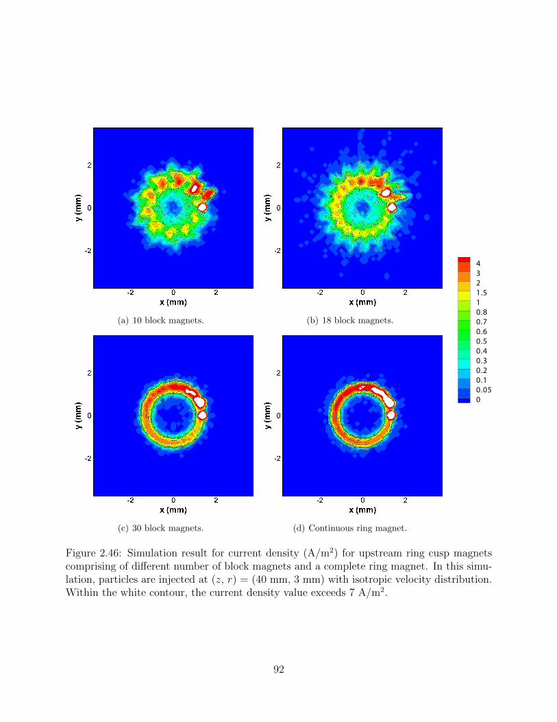
loss structure from the simulation agrees with the experimental result. The large peak near
the center of the magnet is due to the large fraction of primary electrons that are confined
89
(a) (b)
Figure 2.45: Simulation results for (a) primary electron loss positions and (b) contour ofcurrent density at the plane 2 mm upstream of the cylindrical magnet face. The primaryelectron current density exceeds 10 A/m2 within the white contour.
very near the centerline. These electrons stream directly toward the center of the point
cusp without experiencing reflection at the ring cusp field. The simulation result for the
case with xenon pressure of 5 × 10⁻⁴ Torr is similar to Fig. 2.45 except that the ridges
are still observable but not as distinctive as the base pressure case and that the particle
loss positions and current density distribution spread radially outward. This loss structure
disagrees with the experimental result seen in Fig. 2.44. By introducing a xenon gas, primary
electrons can undergo elastic, single and multiple ionization, and excitation collisions with
the background neutrals. If the primary electrons are initiated very close to centerline, they
tend to remain within a small radius and be collected close to the center of the point cusp.
They are unlikely to experience collisions as their path lengths are much shorter than the
collision mean free path. Therefore, the concentrated current near the center should be seen
even for the case of 5×10⁻⁴ Torr if the electron gun and the cylindrical magnet are perfectly
aligned. In contrast, the primary electrons confined by the field lines further away from the
centerline are more susceptible to collisions as their effective path length is increased by the
multiple reflections at the cusps. From these observations, it is possible that elastic collision
causes the significant alternation of the particle guiding center and Larmor radius, and the
90
overall effect is the diffusion in the radially outward direction. The simulation result is
obtained for perfect alignment of the electron gun, test cell, and the downstream cylindrical
magnet: a condition difficult to achieve experimentally. The misalignment can easily cause
the primary electrons that impact at slightly greater radial positions at the collection plane,
and the loss position can move further out due to the radial diffusion once the neutral gas
is introduced. Furthermore, the electric field from the non-quasi-neutral plasma can affect
the primary electron trajectories according to the simulation in Sec. 2.5.2.1. Evidence to the
effect is the substantial increase of total electron current collected inside the discharge by the
introduction of a neutral gas. Unfortunately, the drastic change in the loss structure could
not be self-consistently predicted by the SC model when a degree of misalignment possible
during the experiment was applied.
In order to computationally investigate the ring shape loss structure, primary electrons
are artificially injected with isotropic velocity distribution at the location (z, r) = (40 mm,
3 mm) as illustrated in Fig. 2.43. The simulation focuses on the interaction between the point
cusp magnet and the discrete ring cusp magnets. The purpose is to understand the cause of
the loss structure instead of attempting to determine the exact misalignment conditions in
the experimental data. The effect of other species is neglected in this simulation. Simulations
are conducted by changing the number of block magnets that form the ring cusp immediately
upstream of the point cusp while maintaining constant total magnet volume. Figure 2.46
shows the simulation results for the current density at the collection plane for the case of
10, 18, and 30 block magnets and a radially magnetized ring magnet. The results show that
the ridge structure at the point cusp is caused by the discretation of the upstream ring cusp
as the number of ridges and block magnets correlates. For all the cases, the highest current
density is seen at (x, y) = (∼ 1.4 mm, 0 mm), where the current density is two orders of
magnitude greater than the other peak current density values. This is due to the isotropic
injection of particles at the azimuth angle of 0 leading to a large fraction of electrons with
high parallel velocity that are lost at first incidence to the cusp. Therefore, the peaks are
partially an artifact of the initial velocity distribution and do not influence the interpretation
of the results.
91
(a) 10 block magnets. (b) 18 block magnets.
(c) 30 block magnets. (d) Continuous ring magnet.
4
3
2
1.5
1
0.8
0.7
0.6
0.5
0.4
0.3
0.2
0.1
0.05
0
Figure 2.46: Simulation result for current density (A/m2) for upstream ring cusp magnetscomprising of different number of block magnets and a complete ring magnet. In this simu-lation, particles are injected at (z, r) = (40 mm, 3 mm) with isotropic velocity distribution.Within the white contour, the current density value exceeds 7 A/m2.
92
Numerical and analytical analyses are carried out to explain the loss structure. A counter
clockwise reduction of the current density around the point cusp is seen in both the experi-
mental and computational results shown in Figs. 2.44 and 2.46, respectively. This behavior
is caused by a combination of guiding center drifts in the azimuthal direction and the con-
tinuous electron loss to the cusps upon the localized injection of the particles. Among the
various guiding center drifts, curvature and grad B drifts are found to be the most dominant
types of drift. The velocities for the curvature and grad B drifts are given as
vR =mv‖q
Rc ×B
R2cB
2, v∇B =
mv2⊥
2qB
B×∇B
B2(2.88)
where Rc is the curvature of the field lines. Based on the result obtained by the SC model,
E×B drift is found to be at least an order of magnitude smaller than these drifts. Figure 2.47
shows the azimuthal precession caused by the combination of curvature and grad-B drifts
within each grid region. In this calculation, the gradient of the magnetic field and the radius
of curvature are obtained computationally. Each drift is calculated assuming a pitch angle of
15. At the pitch angle, the curvature drift is an order of magnitude greater than the grad-B
drift, while the effect of grad-B drift becomes more dominant with increasing pitch angle.
z (cm)
r(c
m)
0 1 2 3 40
0.5
1
1.5543210
-1-2-3-4-5
Figure 2.47: Azimuthal precession caused by the combination of curvature and grad-B drifts.Positive sign indicates the direction out the paper, and vise versa. Contour values representthe maximum drift in degrees that an electron can undergo within each grid region. Eachdrift is computed assuming a pitch angle of 15.
93
x (cm)
y(c
m)
-1 0 1
-1
0
1
(a) 10 block magnets
x (cm)
y(c
m)
-1 0 1
-1
0
1
(b) 30 block magnets
Figure 2.48: Particle trajectories of electrons confined between the point cusp and the di-rectly upstream ring cusp comprising of different number of block magnets. Dots aroundcircumference represent location of block magnet center. Particles travel along magneticfield lines and undergo an impulsive turning event at the high drift region.
In Fig. 2.47, electrons confined to the magnetic field lines in between the point cusp and the
directly upstream ring cusp traverse a local region of high curvature and grad-B drift. As
seen in Figure 2.48, confined particles generally travel along the magnetic field lines and only
experience a short azimuthal turning event within the high drift region shown in Fig. 2.47.
Particles that reside radially further and therefore in the regions of lower drift experience a
smaller angular precession per reflection event.
Although it has been shown that the drifts are responsible in the ring loss structure,
they are inadequate to explain the details of the loss structure, particularly the peak and
ridge structure. Here, we will provide a summary of findings that cause such structure; the
detailed explanation is given in Ref. [165]. The peak and ridge structure is caused by a
combination of independent dynamics of electrons. First, the electrons are more susceptible
of losing invariance in the low field regions, becoming less confined when passing through
these regions. The condition for the 1st invariant is assessed using the following equation:
ξ = rL
∣∣∣∣∇BB∣∣∣∣ 1 (2.89)
94
Figure 2.49 highlights the regions where the 1st invariant is the least applicable and conse-
quently where the particles are most likely to become unconfined. In a configuration with a
continuous ring magnet and a cylindrical point cusp magnet, electrons gradually lose their
invariance and are lost to the cusps after experiencing a number of reflections. The region
with higher loss of invariance is still not adequate to explain the peaks for the case of discrete
ring magnets. Indeed, the azimuthal asymmetry of the discrete ring magnets is responsible
in leading the electrons into the low field region. Slight azimuthal gradients in the magnetic
field very near the magnets cause electron drifts in both the positive and negative axial
direction. Since the field lines are highly concentrated near the ring magnets, a slight drift
causes a significant radial translation near the point cusp. The backward axial drift results
in a further penetration of the electron trajectory into the low field region; this causes a
larger degree of loss of invariance and thus leads to the peaks in the loss structure. On the
other hand, forward axial drift translates into significantly larger radius at the point cusp;
this leads to the ridge structure of the loss pattern.
Several possible experimental inaccuracies were investigated to examine the reason for
the discrepancy between the 18 blocks ring magnet and the observed 17 ridges in the results.
Figure 2.49: Validity equation for the 1st adiabatic condition plotting left hand side ofEq. (2.89) for electrons with a 15 pitch angle. Values for different pitch angles are pro-portional to the particle’s perpendicular velocity and thus the Larmor radius. Locations ofgreater numerical value are in greater degree of violation of the invariant condition.
95
4
3
2
1.5
1
0.8
0.7
0.6
0.5
0.4
0.3
0.2
0.1
0.05
0
Figure 2.50: Simulation results for 18 block magnets with the magnet in line with the positivex-axis at 75% magnetization. Results show 17 ridge structures similar to the observation inthe experiment.
One probable explanation is a weakened field at a local azimuthal location. Demonstrated
in Fig. 2.50, the demagnetization of a single block magnet in the array can cause the disap-
pearance of a ridge structure. The variation of angular separation and length of the ridge
structure in the experimental results indicates a non-uniform spacing and/or magnetization
of the block magnets. This uncertainty, coupled with the possibility of a small gap between
the block magnet face and the cylindrical chamber, can potentially create a magnetic field
deficit adequate for similar behavior with the simulation result.
These analyses suggest that the primary electron loss structure is strongly influenced by
the magnetic field upstream of the magnetic cusp. If there is any similarity in the plasma
loss mechanism between a weakly ionized plasma and a sparse plasma, it ultimately suggests
that the loss structure of the weakly ionized plasma may also be affected by the upstream
magnetic field configuration; the conventional theory suggests that the loss width is only a
function of the local magnetic field.
96
2.5.3 Weakly Ionized Plasma
Simulation condition For the simulations described in Secs. 2.5.1 and 2.5.2, the electron
gun was used as a source of high energy primary electrons; the required operating condition
for the gun limited the achievable neutral density and thus the ionization level. For this
reason, the source is replaced with a hollow cathode that is commonly used for the ring-cusp
discharge chamber. The hollow cathode with an orifice of 1 mm in radius is assumed to
operate at 0.4 A discharge current. At the exit of the cathode, it is also assumed that mono-
energetic (8 eV) primary electrons enter the domain uniformly with a cosine distribution for
their velocity directions. As shown in Fig. 2.51, the simulation domain is again inside of a
cylindrical test cell, with a conducting mesh and a plate at the boundaries. The length of the
test cell is determined to ensure that the primary electrons experience sufficient ionization
collision with neutrals. The downstream end plate is biased at 25 V and mesh wall is
grounded. Instead of using the discrete ring magnets, the magnetic field configuration is
made azimuthally symmetric by replacing them with multiple current coils. The magnetic
cusp in front of the cylindrical magnet is still the region of interest. In this simulation, The
neutral flow rate through the hollow cathode orifice is assumed to be 0.6 sccm. The flow rate
and the background chamber pressure of 3 mTorr are used to compute the neutral density
(Fig. 2.52). Neutrals are free to escape through the mesh boundaries, while the sheath near
Source
Figure 2.51: A slice of a cylindrical test cell to be simulated. The region of interest is in frontof the cylindrical magnet placed downstream. Current coils are used to guide the electronsnear the centerline.
97
Figure 2.52: Contour plot of neutral density (m−3). The highest neutral density is at theorigin with the density of > 2.2× 10¹⁹ m−3
the mesh wall prevents plasma electrons from escaping. The neutral density is assumed to
remain constant throughout the simulation since the ion density is a few orders of magnitude
lower than the neutral density, and the reduction in neutral density due to ionization collision
is insignificant.
Analytical Solution for Bulk Density Profile A simple analytical model is developed
to approximate the density profile along the radius where the field is approximately aligned
with the centerline axis. The result from the analytical model described herein is compared
with the computational result for model validation. Assuming that the domain is much
longer compared to the radius, the density profile along the radius can be estimated with
the diffusion equation.∂n
∂t−D∇2n = n(r) (2.90)
The first term in Eq. (2.90) is neglected since the solution of interest is steady-state. In this
formulation, it is assumed that the magnetic field is homogeneous away from the magnetic
cusp in the direction parallel to the axis. Assuming that the ion generation rate density
profile along the radius can be expressed by a polynomial of degree Nd, the equation to be
solved becomes,
−D⊥1
r
∂
∂r
(r∂n
∂r
)= n(r) =
Nd∑s=1
psrNd−s (2.91)
98
where p is the polynomial coefficients. At the edge of the sheath near the side wall, the
characteristic loss velocity of ions, uw is assumed to satisfy the Bohm criterion for a positive
sheath, uw = uBohm =√kTe/mi. Thus, the boundary conditions are,
n(r = rmax) = nw, Γ = −D⊥∂n
∂r
∣∣∣∣r=rmax
= nwuw (2.92)
The solution of Eq. (2.91) is then,
n(r) =
Nd∑s=1
ps(Nd − s+ 2)2
[r
(Nd−s+2)max − r(Nd−s+2)
D⊥+r(Nd+s+1)
uw(Nd − s+ 2)
](2.93)
A similar solution can be derived using a boundary condition with n(r = rmax) = 0, yielding
Eq. (2.93) without the second term in the parentheses. Equation (2.93) is dependent on the
perpendicular diffusion coefficient, D⊥, which is difficult to obtain for our specific problem.
The classical ambipolar diffusion across a magnetic field can be obtained by equating the
ion and electron fluxes perpendicular to the direction of magnetic field. [166]
D⊥ =µi⊥De⊥ − µe⊥Di⊥
µi⊥ − µe⊥(2.94)
The diffusion coefficient given in Eq. (2.94) is appropriate in a infinitely long cylindrical
plasma with uniform magnetic field along the axis. When the domain is finite and is bounded
by conducting walls, the diffusion coefficient should be modified to take into account of
Simon’s “short-circuit” effect [167].
D⊥ =µiDe⊥ − µeDi⊥
µi − µe(2.95)
Unlike the case with the classical ambipolar diffusion, the particle flux is no longer at the
same equilibrium value in each direction, but rather the total flux for each species should
be maintained. In our problem, strong and weak cusps are placed at the downstream and
upstream ends, respectively. In this magnetic field configuration, electrons are not freely lost
to the ends if they are confined near the centerline. In contrast, the electrons are easily lost
99
at the ends away from the centerline due to the low field strength. Therefore, the diffusion
coefficient applicable for our problem is likely between Eq. (2.94) and Eq. (2.95), and the
density solutions obtained using the two diffusion coefficients should provide the upper and
lower bounds for the computational result.
Numerical Results Unfortunately, the solution did not converge at the end of simulation
as shown in Figs. 2.53 and 2.54. The species densities were nearly steady-state, but the
ion and plasma electron densities did not meet the convergence criteria near the end of
Figure 2.53: Maximum and volume averaged densities versus iteration. The densities weremixed with values from 25 previous iterations.
50 100 150 200 250 300 3500
100
200
300
400
500
600
700
800
900
1000
Iteration Number
Ele
ctric
Pot
entia
l (V
)
MaximumVolume−Averaged
Figure 2.54: Maximum and volume averaged electric potential versus iteration. The valueswere obtained directly from potential solver (before performing mixing with potential valuesfrom 25 previous iterations).
100
simulation. Note that the simulation was restarted at iteration 163. The electric potential
was far from convergence; the max potential was greater than 200 V, while we expected
that the maximum and volume averaged potential should be close to the expected plasma
potential of ∼ 33 V.
Figure 2.55 compares the computational and analytical results for a density profile along
the radius at z = zmax/2. The profile for ion generation rate density is obtained by the
computational model and is fitted with a polynomial of degree Nd = 9. As seen in Fig. 2.55,
the computational result does not agree well with the analytical solution; we expect that
the computational result would be bounded by the profiles predicted using ambipolar and
Simon’s diffusion coefficients. One of the reasons for the disagreement may be that the
electric potential has not been developed completely at the end of simulation. For the
profile shown in Fig. 2.55, a converged solution for the electric field is expected to act to
push the ions near the centerline further radially outward, so the density profile is flattened.
Comparing the computational results in the middle and at the end of simulation, the slope
of the density profile became closer to the analytical solution; however, further iterations
did not result in the expected density profile. Another source of the error can be the finite
dimension of the domain. The transport in the axial direction is neglected in the analytical
0 2 4 6 8
1014
1016
1018
Radial Positon (cm)
Pla
sma
Den
sity
(m
−3 )
Computational at end of simulationComputational at intermediate iterationAnalytical, Ambipolar & n(rmax)=nw
Analytical, Ambipolar & n(rmax)=0Analytical, Simon & n(rmax)=nw
Analytical, Simon & n(rmax)=0
Figure 2.55: Comparison of density profiles from computational and analytical models alongthe radius at z = zmax/2.
101
model; however, a finite diffusion in axial direction must be present even at z = zmax/2 since
the domain radius is only a third of the length. The computational model predicted slight
variation of density axially near the axis while relatively larger density variation was seen
further away from the axis. Finally, azimuthal inertia terms in the diffusion equation are
neglected in the analytical formulation which may be significant.
Since the solution did not converge at the end of the simulation, the results are inaccurate
but do exhibit some physical consistencies when comparing the potential structure and the
relative species density distributions. Figure 2.56 shows the potential structure near the cusp.
The contour level is omitted as the magnitude is not of importance here, but red corresponds
to high potential and blue corresponds to low potential. It is clearly seen that there is a
sheath along the anode wall as represented by the steep drop of the potential toward the
wall. Figure 2.57 compares the species densities near the cylindrical magnet cusp. The right
hand side of the domain shown in Fig. 2.57 represents the anode wall at the magnetic cusp;
the magnet face is 3 mm downstream of this surface. The general and relative structure of
the density profiles shown in these plots remained unchanged toward the end of simulation.
Figure 2.56: Electric potential near the anode wall at the magnetic cusp. Magnet face is atz = 310 mm. Sheath is developed along the anode wall.
102
z (mm)
306 306.5
Ion
306 306.5
2.0E +17
1.0E +17
5.0E +16
4.5E +16
4.0E +16
3.5E +16
3.0E +16
2.5E +16
2.0E +16
1.5E +16
1.0E +16
5.0E +15
P l a s m a
E l e c t r o n
r(m
m)
306 306.50
0.5
1
1.5
2
2.5
P r i m a r y
E l e c t r o ntext
Figure 2.57: Species densities (m−3) very near the cusp. Magnet face is at z = 310 mm.Primary electrons are confined very near the centerline.
Since the hollow cathode is placed along the same axis as the cylindrical magnet, the primary
electrons are directed toward the cusp and are confined very near the centerline. Primary
electrons are not as confined by magnetic mirroring and sheath as plasma electrons, so the
residence time of primary electron is a few orders of magnitude less than that of plasma
electron. Therefore, it is much more difficult for the primary electrons to diffuse across the
magnetic field. Because of the concentrated primary electron population near the centerline,
the potential is developed to attract ions radially inward. The radial component of the
electric field interacts with the axial magnetic field to create an azimuthal E×B drift for the
highly confined plasma electrons. Ions and plasma electrons are predominately created by
inelastic collisions between primary electrons and neutrals, so their generation rate density is
high in the region of high primary electron density. Ions created very near the magnetic cusp
are immediately accelerated toward the wall whereas plasma electrons are repelled from the
wall. As the plasma electrons are strongly confined by the magnetic field and sheath, these
results suggest that their path length is to be over 50 times longer than that for primary
electrons. The plasma electrons diffuse much further radially outward due to multiple elastic
collisions with neutrals and eventually gain enough parallel velocity to reach the anode wall.
103
As a result, it appears that they are mainly collected in an annular region surrounding the
axis near the cusp. Consequently, these results suggest that in the near-sheath and sheath
region near the axis may be dominated by the primary electrons and ions while the plasma
electrons and ions occupy the outer region at low primary electron density. These results do
not agree with measurements in spindle cusp and picket fence experiments [89–92] and may
be attributable in part to the current lack of a converged solution. We wish to note, however,
that in contrast to the experiments mentioned the cusp here occurs at a current collecting
wall. The electric field at the wall must be such that a sufficient current of electrons is drawn
to maintain the discharge. If the electron current near the cusp is ample, one may expect
the normal sheath formation as electrons are lost rapidly along the field lines. The different
boundary conditions here may reasonably be expected to result in different distributions.
Figure 2.58 shows the local degree of quasi-neutrality, η, obtained by the computational
result where η is given as,
η =ni − ne
max(ni, ne)(2.96)
z (mm)
r(m
m)
303 304 305 3060
1
2
3
4
1.00.80.60.40.20.0
-0.2-0.4-0.6-0.8-1.0
Figure 2.58: Degree of quasi-neutrality obtained by η = (ni− ne)/max(ni, ne). Magnet faceis at z = 310 mm. Positive and negative contours indicate regions dominated by ions andelectrons, respectively.
104
Here, η = 0, η > 0, and η < 0 indicate quasi-neutral, ion-dominated, and electron-
dominated plasma, respectively. As shown in Fig. 2.58, ions dominate the near-wall region
at r & 1.6 mm. This is, again, due to the sheath potential that accelerate ions toward
the wall and repel plasma electrons away from the wall. Within the near-wall region at
r . 1.6 mm, the positive sheath is still present, but the difference between the plasma and
anode potential is not large enough to prevent primary electrons from being lost at the wall.
As a result, ions in this simulation respond to the potential structure caused by the high
primary electron concentration. However, they do not reside in the region long enough to
completely counteract charge imbalance, being accelerated toward the wall by the sheath.
Therefore, the region very near the centerline is dominated by the primary electrons.
2.6 Chapter Summary
The SC model that uses an iterative Monte Carlo technique has been developed to investigate
the important structure and dynamics of the cusp confined plasma species. The model uses
various numerical techniques that are necessary for our objective. These include implemen-
tations of analytical equations for magnetic fields induced by permanent magnets together
with the fast computation methods for elliptic integrals (Sec. 2.3.2 and Appendix C) and
the modified Boris method for integration of particle motion (Sec. 2.3.3). In addition, we
have developed the particle weighting algorithm (Sec. 2.3.4) and the second order electric
field solver (Sec. 2.3.7) that work for any type of mesh including an adaptive regular and a
MFA mesh during the course of the model development. Furthermore, advanced methods
for calculations of collisions (Sec. 2.3.5) and electric potential (Sec. 2.3.6) and also a method
for smoothing (Sec. 2.3.8) are implemented in the SC model. All of these methods have
been validated independently in simple test cases, while this chapter has provided extensive
validation studies for the particle weighting algorithm, the potential solver, and the electric
field calculation.
The simulation using the SC model began with the simplest system that involves a
magnetic cusp: 25 eV primary electrons from an electron flood gun shot toward a point-
105
cusp cylindrical magnet placed downstream. The simulation result showed good qualitative
and quantitative agreement with the experimental data, thus further validating the particle
tracking and magnetic field calculations.
Then, the simulation was extended to include multiple species (primary electrons, neu-
trals, ions, and plasma electrons) to examine their interactions, especially in the cusp region
very near the anode wall. The sparse plasma condition was achieved by adding multiple ring
cusps in an effort to confine primary electrons and the other plasma species. The results
from the multi-species computational simulations provided insight into the dynamics and
structure of sparse plasma in the cusp region and showed that the sparse plasma conditions
used in this experiment do not exhibit the same mechanisms that are used to explain the
hybrid gyro behavior for a more highly ionized plasma. In particular, the reduction of ion
loss width was due to the high rate of generation near the cusp and the potential structure
that immediately accelerated ions toward the electrode. On the other hand, the plasma
electrons immediately repelled from the wall due to the electric field are confined by the
potential and the magnetic field, experiencing multiple elastic collisions with neutral atoms
and thus resulting in the expansion of plasma electron volume and the increase in the loss
area.
The next simulation for the sparse plasma in the multi-cusp configuration focused on
the dynamics of the primary electrons. The experimentally measured loss pattern exhibited
an interesting pattern with the peak and ridge structure with decreasing current density in
the counter clockwise direction. The SC model was applied to provide a phenomenological
investigation of the loss pattern by injecting the primary electrons between the point cusp
magnet and the ring magnets directly upstream of the point cusp. Ignoring the peaks near
the injection point that are artifacts of the initial velocity distribution, all the important
features of the experimentally measured loss pattern were captured by the model, leading
to the conclusion that the unique pattern was indeed due to the upstream discrete block
magnets creating the ring cusp. Analytical study was carried out, and it was found that the
loss structure was due to a combination of azimuthal drift in the low field region, forward
and backward axial drifts very near the ring cusp, and the loss of invariance in the low field
106
region. This indicated that the primary electron loss structure was strongly affected by the
upstream magnetic field configuration. Tying with the results from the full simulation for
the sparse plasma, the loss of the sparse plasma should be altered by changing the upstream
magnetic field configuration, while this does not necessarily apply to a weakly ionized plasma.
The SC model was also used to simulate a weakly ionized plasma in a field configuration
created by multiple current coils and a cylindrical magnet. Due to the structure of the
model, it was found that the convergence condition was extremely difficult to satisfy due to
the opposite charges of ions and electrons. Even by implementing a high degree of mixing
between iterations, the electric potential still oscillates from iteration to iteration. The
quasi-neutral condition for a weakly ionized plasma requires the charge density to be within
∼ 1011 m−3 which corresponds to ∼ 10−4 % of the species density for this specific simulation
condition. Since the solution did not converge at the end of the simulation, the results
were inaccurate but did exhibit some physical consistencies when comparing the potential
structure and the relative species density distributions. In particular, the sheath structure
near the anode wall was captured, and the plasma species distribution very near the magnetic
cusp was resolved.
107
CHAPTER 3
Techniques for a Ring-Cusp Discharge Chamber
Modeling for a Micro-Discharge Design
The objective of this effort is to use the ring-cusp discharge chamber model developed by Wirz
and Katz [13, 24] (DC-ION) to address the design and optimization challenges of miniature
to micro discharges on the order of 3 cm to 1 cm in diameter. To this end, significant
improvements to the model are necessary due to the scaled-down dimension of the domain.
The SC model and the related experiments discussed in Chapter 2 have revealed important
phenomenological primary electron loss behavior that is strongly affected by the upstream
magnetic field, which needs to be extended for a weakly ionized plasma. While the SC model
has provided a qualitative description of plasma structure near the cusp, it still requires
many improvements to obtain a fully converged solution and thus provide a precise and
quantitative picture. With the lack of accurate descriptions, the formulation of a theory that
could be easily included in DC-ION was not possible. Nevertheless, improved techniques and
routines that can be incorporated in DC-ION have been developed to achieve better accuracy
and computational speed. Some of these are also necessary to enable simulations for small
scale discharges. Several components of the SC model can be used in DC-ION such as
the analytical equations for permanent magnets, the particle weighting algorithm, and the
electron-atom elastic scattering. This chapter discusses the other improved techniques and
routines to be incorporated in DC-ION. First, a brief description of DC-ION is provided in
Sec. 3.1. Section 3.2 gives the details of the magnetic field aligned (MFA) mesh generation
process. Section 3.3 describes the numerical method for solving the plasma diffusion equation
in such a complex mesh and compares the solutions obtained with the MFA and uniform
meshes. Finally, Sec. 3.4 discusses the improvement made to the neutral density calculation
108
method in terms of computational efficiency. Both Secs. 3.2 and 3.3 are taken from the
article Magnetic Field Aligned Mesh for Ring-Cusp Discharge Chambers presented at 50th
AIAA/ASME/SAE/ASEE Joint Propulsion Conference.
3.1 General Description of a Ring-Cusp Discharge Model
The discharge chamber model developed by Wirz and Katz [13, 24], DC-ION, is the 2D/3D
hybrid fluid/particle model that self-consistently includes effects of primary electrons along
with other plasma species. The model has been validated against the data for the NSTAR
ion thruster with 30 cm chamber diameter and also applied to the simulation of 3 cm MIXI
thruster. The general structure of the model is shown in Fig. 3.1. As shown in Fig. 3.1, the
model consists of the Internal Mesh Generator and four sub-models. In the Electron Collision
Sub-Model, the Monte Carlo approach is used for primary electrons, tracking many macro-
particles representing a number of electrons in 3D domain. This sub-model is similar to
Inputs
Geometry, Temperatures,
Boundary Conditions
Electron Collision Sub-Model
Neutral Atom Sub-Model
Internal Mesh Generator
Results
Ion Diffusion Sub-Model
Electron Thermal Sub-Model
Operating Conditions
Figure 3.1: General structure of DC-ION. Reproduced from Ref. [24].
109
the SC model discussed in Chapter 2; thus, the more sophisticated numerical techniques
and methods can be directly applied to the sub-model for improvements. The Ion Diffusion
Sub-Model solves the plasma diffusion equation derived from the conservation equations for
mass and momentum for ions and plasma electrons. Then, the electron energy equation
is computed in the Electron Thermal Sub-Model to obtain the electron temperature. The
neutral density is computed using the zonal method in the Neutral Gas Sub-Model. In this
model, a regular grid with uniformly sized rectangular elements is generated by the Internal
Mesh Generator. The techniques and routines discussed in this chapter are related to the
Internal Mesh Generator, the Ion Diffusion Sub-Model, and the Neutral Atom Sub-Model.
3.2 Magnetic Field Aligned Mesh
3.2.1 Introduction
In a magnetized plasma, rates of transport in directions parallel and perpendicular to a
magnetic field are different. According to the classical plasma transport theory, the perpen-
dicular electron transport coefficient is scaled with B−2 and is always smaller, and often at
least an order of magnitude smaller, than the parallel transport coefficient [141]. This is
also commonly the case even when one considers more Bohm-like (B−1) diffusion. When
computationally solving the transport equation for such systems, a numerical error arises
due to the anisotropicity of the transport coefficients if the computational grid is unaligned
with the magnetic field; this is called the numerical diffusion. For example, Anderson [168]
demonstrated an artificial diffusion of the temperature by solving the heat conduction equa-
tion on a 2D Cartesian grid with the magnetic field at 45 with respect to the grid edge.
Even by setting the perpendicular conductivity to zero (anisotropy ratio of ∞), the tem-
perature field after 35 time-step showed a finite perpendicular heat flow, which resulted in
the effective anisotropy ratio of ∼4. A similar but more extensive study was performed by
Meier et al. [169] by solving the heat conduction equation with a high-order finite element
code. They found that even a small misalignment can cause a significant numerical error
and that the error can be reduced by using a finer resolution and a higher-order polynomial
110
basis expansion in the finite element method. They also noted that the accuracy is slightly
better if the misalignment between the field and the grid was 45 as opposed to some other
non-zero angles.
One of the methods to remedy the numerical diffusion error is to use a computational
grid that is aligned with the magnetic field. The generation of the magnetic field aligned
(MFA) mesh is most commonly done by simply tracing the field lines [23, 170–179]. Given
the data or the functional form of the field lines, the lines parallel and orthogonal to the
magnetic field are determined by the direct numerical integration; the integration can be
executed using commercially available graphics software [170, 171] or an explicit method
such as 5th order Adams-Bashforth method [177–179]. Once the intersections of those lines
are determined, the computational mesh can be generated by connecting the intersections
such that each grid element consists of facets parallel and perpendicular to the field lines. The
direct numerical integration is very easy to perform and can be applied to a complex system
where a transformation between the magnetic flux coordinate and inertial coordinate cannot
be defined. However, the method is often too time-consuming as the step-size has to be very
small to obtain enough accuracy in the line integration. For 3D plasma edge modeling of
toroidal fusion devices, the time required in generating a MFA mesh is significantly reduced
by using mapping techniques after a block of 3D mesh covering some toroidal angles is
generated [174–180]. These mapping techniques are not applicable for the field configuration
in a ring-cusp discharge chamber. In contrast to the numerical integration method, the lines
of magnetic field can be determined directly if there exists an appropriate transformation
between the magnetic flux coordinate and inertial coordinate. Magnetic field lines are simply
represented by the lines of constant flux function, ψ, which can be computed numerically.
This method has been applied by Brieda and Keidar [181] for Hall-effect thruster simulations
and by Marchand and Dumberry [182, 183] for 2D edge plasma modeling. The mapping
method described by Abdullaev [184] may also be applied for a toroidal system.
In a DC ring-cusp ion thruster, the magnetic field topology is fairly complex. The
magnetic field is created by multiple block magnets that are placed along the circumference
of the discharge chamber to create a ring-cusp field. Near the magnetic cusp, the magnetic
111
field is highly convergent, and the gradient of the field is very high. Furthermore, the
field configuration typically consists of a null point where the magnetic field cancels out to
zero. Considerably large difference between the maximum and the minimum magnetic field
strengths generally makes the task of MFA mesh generation more difficult. In addition,
two field lines intersect at the null point; therefore, a special treatment of the null point
may be required. Wirz and Katz [23, 172] successfully generated and applied the MFA
mesh for the simulation of NSTAR discharge chamber. The MFA mesh generation was
accomplished by tracing the magnetic field lines starting from the boundary near a magnet.
In later simulations, they switched to a uniform mesh due to the inability of their MFA mesh
algorithm to quickly adapt to changing magnetic field structures [185].
This section provides the detailed descriptions of a 2D axisymmetric MFA mesh gener-
ation method. The algorithm is significantly robust to automatically mesh a wide range of
magnetic field geometries without the need for significant user input. Existing commercial
meshing software is not adequate in accomplishing the task because much control in mesh
generation is necessary; the MFA mesh with a fair grid quality typically requires adjustment
of grid especially in the near-boundary region, and the appropriate technique may differ from
configuration to configuration.
3.2.2 Process of MFA Mesh Generation
The procedure in the generation of a MFA mesh used in this section involves primarily six
steps: (1) solve for stream function and scalar potential, (2) identify null points, (3) select
contour levels, (4) extract node points, (5) create cell elements, and (6) improve the mesh
quality. Each mesh generation step is discussed in detail here. Instead of directly tracing
the magnetic field lines and lines orthogonal to the field, we solve for the stream function
and scalar potential directly from the appropriate relations between the two functions and
the magnetic field. This method is computationally much less expensive than tracing the
field lines. The transformation from the physical coordinate to the flux coordinate is greatly
simplified if the problem is two dimensional or three dimensional with some symmetry.
112
Therefore, the ring-cusp block magnets are approximated as a single ring magnet. The
error in the field strength associated with this approximation was investigated by Mao [186]
for a configuration with three ring-cusps. The largest error was seen near the magnets at
the off-face place due to the lack of magnet material, but the error was within 5 % while
the error away from the magnet was well below 1 %. Furthermore, the numerical method
described in Sec. 3.3 does take into account the misalignment of the grid with the field, so
the exact alignment of the mesh with the field throughout the domain is not required. The
MFA mesh generation method described herein requires a fine uniform mesh so that the
stream function and scalar potential values can be numerically evaluated on the grid points.
The accuracy in the alignment and the speed in the grid generation are dependent on the
resolution of the uniform mesh. In this study, we use the number of cells in the range of 100
to 400 in each direction. This provides a reasonably accurate calculations with an acceptable
computational run-time.
3.2.2.1 Stream Function and Scalar Potential
Knowing the magnetic field at the nodes of the fine uniform mesh, the stream function and
the scalar potential can be determined computationally from the equations derived in this
section. This step can be skipped if one can derive functional forms of the stream function
and the scalar potential that describe their variations within the computational domain.
However, such functions are nearly impossible to obtain for the magnetic field created by
the permanent magnets as the field equations are relatively complex. Therefore, we evaluate
the two functions digitally onto the fine uniform mesh. This idea came from the work by
Mao [186] but with a slightly different formulation. Since the magnetic field is divergence-
free (∇ ·B = 0), there exists a vector field A such that B = ∇×A. For the axisymmetric
magnetic field (B = Bz z + Brr), A must be in θ-direction and is expressed as Aθ = ψ/r.
Taking the curl of A and equating with B, the relation between the stream function and
magnetic field can be obtained.
Bz z +Brr =1
r
∂ψ
∂rz − 1
r
∂ψ
∂zr (3.1)
113
By replacing the magnetic field with the flow velocity, Eq. (3.1) becomes the well-known
relation for the Stokes stream function that is used to describe the streamlines and flow ve-
locity in a 3-D incompressible flow in a cylindrical coordinate system. Finally, by multiplying
both sides by r in Eq. (3.1) and taking the curl from both sides, the equation becomes the
Poisson’s equation.∂2ψ
∂z2+∂2ψ
∂r2= − ∂
∂z(rBr) +
∂
∂r(rBz) (3.2)
Similar approach can be made to deduce the equation for the scalar potential. In the absence
of external currents and time-varying electric field, ∇ × B = 0 according to the Maxwell
equation. This implies that the scalar potential, φ, can be employed such that B = ∇φ.
Taking the divergence from both sides, the equation becomes the Poisson’s equation similar
to Eq. (3.2).∂2φ
∂z2+∂2φ
∂r2= −1
r
∂φ
∂r= −Br
r(3.3)
The stream function and scalar potential values at the fine uniform grid points can easily be
obtained by solving Eqs. (3.2) and (3.3) using the standard finite difference method. The
stream function can be used to compute the volume flux through the flux surface bounded
by a constant value of ψ by 2πψ. On the other hand, the scalar potential values do not have
any direct physical meaning. The zero value can be set arbitrarily as for the electric and
gravitational potentials. We typically choose the zero value to be at the location where the
magnitude of the radial magnetic field is the minimum along the side wall of the cylindrical
domain.
3.2.2.2 Null Point
Before proceeding to the actual construction of the grid, all the null points within the
discharge chamber are determined by finding the local minima of the magnetic field strength.
The number of null points is usually less than or equal to the number of ring magnets.
Therefore, the speed in determining the null points is not an issue as long as a reasonable
number of ring magnets is used. The local minima are determined by the method of steepest
descent [187]. Given an initial position as an input, the position is simply advanced in the
114
direction of the magnetic field strength gradient until the gradient becomes effectively zero.
xh+1 = xh − t∇|B||∇|B||
(3.4)
where x is the position and t is the step size. The gradient of the magnetic field strength is
approximated by the difference equation.
∇|B(z, r)| = |B(z + ε, r)| − |B(z, r)|ε
z +|B(z, r + ε)| − |B(z, r)|
εr (3.5)
where ε is a very small number which we set to the square root of the machine epsilon.
When the position reaches the domain boundary, the gradient in the direction normal to the
boundary is set to zero to ensure that the advanced position is always within the domain. The
step size, h, is initially set to a relatively large number, e.g. 1/20 of the maximum dimension
of the domain, to increase the speed of convergence. When the position is sufficiently close
to the location of the local minimum, the position starts to oscillate, going back and forth
and never reaching the exact location of the minimum. Therefore, the step-size is gradually
reduced by an order of magnitude every time the positions at hth and h-2th steps are too
close (i.e. |xh − xh−2| < 0.1t) until the advancement in position is less than the machine
epsilon. This ensures an accurate determination of the null points.
3.2.2.3 Selection of Contour Levels
The lines of constant stream function represent the magnetic field, while the lines of constant
scalar potential represent the lines orthogonal to the magnetic field. A set of these lines are
chosen to generate the MFA mesh. In a contour plot, contour lines correspond to lines
of constant function values, and the process discussed here can be thought to be simply
adjusting the contour levels. The selection of the contour levels for the stream function and
the scalar potential is directly related to the resolution and the quality of the MFA mesh.
The element size near the magnet is generally finer than the elements in other regions because
of the very strong field strength and the converging field structure. On the other hand, the
115
element size near the null point is always the largest. The large element in the region can
affect the overall accuracy of the solution. Therefore, the method for choosing the contour
level can be critical. Different functions can be used for the contour level selection, while
the choice of the appropriate function strongly depends on the magnetic field configuration:
particularly, the ratio of the maximum strength to the minimum strength.
Given the number of contour levels for the stream function nψ, we first determine the
index, p0, so that p0-th level corresponds to ψ = 0.
p0 = int
(nψ
ψmin
ψmax − ψmin
)(3.6)
where ψmax and ψmin are the maximum and the minimum stream function values. The level
indices greater and lower than p0 are for positive and negative ψ levels, respectively. Then,
the contour levels are chosen based on the exponentially stretching function from ψ = 0
to positive and negative ψ. Even with the function, the jump in the contour level from
ψ = 0 to the next level is too large for most of the configurations tested. In other words,
the smoothness of the grid from the innermost element to the adjacent element in the radial
direction would not be preferable. Therefore, we add another level after the level of ψ = 0.
This is done by first determining the levels ψp0+2 and ψp0−2 that correspond to the first levels
if we were to only use the exponential stretching function.
ψp0+2 = ψmax
exp(
1nψ−p0
αψ
)− 1
exp (αψ)− 1, ψp0−2 = ψmin
exp(
1p0−1
αψ
)− 1
exp (αψ)− 1(3.7)
where αψ is the stretching parameter for ψ specified as an input. Then, ψp0+1 and ψp0−1 are
chosen simply by taking a fraction of ψp0+2 and ψp0−2, respectively.
ψp0+1 = γ+ψp0+2, ψp0−1 = γ−ψp0−2 (3.8)
where γ+ and γ− are less than 1 and are also specified as inputs. The rest of the contour
116
levels are determined by the exponentially stretching function.
ψp = ψp0+2 + (ψmax − ψp0+2)
exp(
p−p0−2nψ−p0−2
αψ
)− 1
exp (αψ)− 1if p > p0 + 2
ψp = ψp0−2 + (ψmin − ψp0−2)exp
(p0−2−pp0−3
αψ
)− 1
exp (αψ)− 1if p < p0 − 2
(3.9)
For the scalar potential, q0 is determined in the same manner as Eq. (3.6) such that φq0 = 0.
However, the contour levels are determined solely with the exponentially stretching function.
φq = φmax
exp(
q−q0nφ−q0
αφ
)− 1
exp (αφ)− 1if q > q0
φq = φmin
exp(q0−qq0−1
αφ
)− 1
exp (αφ)− 1if q < q0
(3.10)
where αφ is the stretching parameter for φ specified as an input. In order to reduce the
element size at a null point, we choose the null point to be a node. This is ensured by
replacing the ψ and φ contour levels that are the closest to the values at the null point (ψnull
and φnull) with those values. Even with the determination of contour levels by Eqs. (3.8)
and (3.9), the resolution near the domain axis may still be undesirable. This condition occurs
when the ratio of the maximum to the minimum magnetic field strength is large: more
specifically, when a magnet is placed too close to the boundary in a ring-cusp discharge
chamber. In this case, we simply manipulate those large elements rather than trying to
control them directly by Eqs. (3.8) and (3.9). The mesh is first constructed with a simple
stretching function for ψ similar to Eq. (3.10), which results in an even larger element size
near the domain axis. After the baseline mesh is constructed, the near-axis elements are
split into multiple elements.
117
3.2.2.4 Determination of Node Points
The nodes are simply placed at the intersections between the stream function and the scalar
potential contour lines that are determined based on the set of levels we specified previously.
Based on ψ and φ that are computed using Eqs. (3.2) and (3.3) on the uniform mesh, we use
the marching squares algorithm to approximate the contour lines. Each cell of the uniform
mesh has four corners with ψ and φ values stored. The locations where the ψ and φ contour
lines intersect with each cell boundary are determined by linear interpolation using the ψ and
φ values stored at the ends of the cell facet (Fig. 3.2(a)). The number of intersections with the
cell of the uniform mesh is always an even number (most likely two) as a contour line cannot
terminate within a cell. All the segments of the contour lines within a cell are approximated
as straight lines (Fig. 3.2(b)). If the contour lines for both ψ and φ are through the cell,
there is a possibility that the two lines intersect within the cell. The intersection condition
is checked by comparing the location of the four points and then utilizing the cross-product.
Once we find that the two lines intersect, the determination of the intersection point is trivial
(Fig. 3.2(c)). This process is repeated for all the cells in the uniform mesh. After all the
interior nodes are located, then the nodes at the domain boundaries are determined. Unlike
the case for the interior cells, the intersection with any contour line with a domain boundary
is located using linear interpolation. Finally, additional information such as the indices for
ψ and φ levels and the connectivity between nodes is stored to be utilized in the creation
(a)
ψ
φ
(b)
ψ
φ
(c)
Figure 3.2: Process of node creation. (a) The intersections of the ψ and φ contour lines withthe cell boundaries are determined using linear interpolation. (b) The contour lines withinthe cell are approximated as straight lines. (c) A node is placed at the intersection of thecontour lines.
118
process of the MFA mesh elements. The connectivity information is based on the levels for
the ψ and φ contours and the distance. Any interior node, except the null node, with contour
levels of (ψp,φq) has four adjacent nodes with levels of (ψp,φq+1), (ψp+1,φq), (ψp,φq−1), and
(ψp−1,φq). In many configurations, there exist multiple nodes with the same ψ and φ levels
within the entire domain, and the appropriate adjacent node is chosen by comparing the
distances between the nodes.
3.2.2.5 Creation of Cell Elements
Once all the node points are determined, these nodes need to be connected properly to create
the MFA mesh elements. The process of the element creation involves tracing of the node
points based on the node connectivity information to find a polygon that does not enclose
any other node point. Starting from one interior node that does not correspond to a null
node, we move along the adjacent nodes in the counterclockwise direction in ψ-φ coordinate
system (e.g. in the order of (ψp,φq), (ψp,φq+1), (ψp+1,φq+1), and (ψp+1,φq)) until reaching
the initial node of each tracing (Fig. 3.3(a)). As there are four adjacent nodes associated
with the interior node, the tracing for one interior node is done four times, each time first
going to a different adjacent node. Although tracing four times for each interior node is often
redundant and results in multiple-counting of the same element, this ensures no miscounting
of the MFA mesh element. Special treatment has to be made for the case of the null node
and the boundary node during the process of node tracing. At the null node, there are
always two possible choices for the next node; there is a total of eight nodes adjacent to the
null node with four pairs of nodes at the same level of ψ and φ (Fig. 3.3(b)). For boundary
nodes, simply going along the nodes with the four combinations of ψ and φ levels cannot
be applied because the domain boundary typically cuts through the quadrilateral MFA cell
element, resulting in irregular elements with the number of facets ranging from three to six.
Therefore, we take into account the physical location of nodes in addition to the ψ and φ
levels. Starting from a node j−1 during the node tracing process, let the first adjacent node
be a null node or a boundary node j. Then the next node j+1 is determined by choosing an
adjacent node that gives the smallest positive angle in counterclockwise direction between
119
pψ
1pψ +
1pψ −
qφ
1qφ +
1qφ −
(a)
a
b
1θ2θ
1( , )qp
ψ φ−
1( , )qp
ψ φ−
1( , )qp
ψ φ+
1( , )qp
ψ φ+
1)( ,p q
ψ φ + 1)( ,p q
ψ φ +
1)( ,p q
ψ φ −
1)( ,p q
ψ φ −
( , )qp
ψ φ
(b)
Figure 3.3: Creation process of a MFA mesh element. (a) Nodes are traced in the counter-clockwise direction in ψ-φ coordinate system. (b) Choosing the appropriate next node froma null node by comparing the angles.
two vectors, a = xj−xj−1 and b = xj+1−xj. The angle can easily be determined by utilizing
the dot product and the cross product.
After creating the MFA mesh elements with appropriate nodes associated with them,
the rest is a matter of cleaning up the information stored in the element data structure and
obtaining additional information that can be useful in the actual computation of a solution
with the mesh. The node numbers stored in each element is reordered in the counterclockwise
order. First, we find the node that is the closest to the origin. Then, the next node is chosen
by the smallest positive angle in counterclockwise direction using the dot product and the
cross product between the vectors, a and b, as defined previously. When the second node
is to be determined, vector a is chosen to be a = −εz − εr − x1 where ε is a very small
number greater than zero; this ensures a 6= 0 when at the origin. The additional information
to be stored includes elements attached to a node and elements adjacent to an element.
The information can easily be obtained by the node numbers stored for each element. For
example, an element adjacent to the element of interest can be found by finding an element
that shares the same two nodes. Finally, boundary elements are added at the midpoints of
two adjacent boundary nodes. The boundary elements are used to simplify the numerical
procedure in computing the solution.
120
3.2.2.6 Post Processing: Improvements on Mesh Quality
The procedure described above is sufficient to generate a MFA mesh that can be used for a
plasma simulation in a magnetic field. However, the MFA mesh does not always produce a
result that is more accurate than a solution obtained with a uniform mesh, especially for a
complex magnetic field configuration. The accuracy of the numerical solution is dependent
on many factors including the problem to be solved, the mesh quality, and the alignment
of the mesh [188]. The quality of a mesh is often determined by geometric factors such as
smoothness, aspect ratio, and skewness [189, 190]. The smoothness describes the degree of
change in element sizes. A large jump in size from an element to its neighboring element
is typically not preferable. On the other hand, the aspect ratio is simply the ratio of the
maximum to the minimum element edge length, and the skewness is based on the maximum
and the minimum interior angles of an element. Mesh elements with the similar edge lengths
and the similar interior angles are often preferable for a better mesh quality. The MFA mesh
sacrifices the mesh quality to achieve the alignment with the magnetic field. The inaccuracy
in the numerical solution using the MFA mesh is likely caused by the poor mesh quality
near the simulation boundaries. The domain boundary always cuts through a quadrilateral
element that has two facets parallel to and the others perpendicular to the magnetic field.
While the elements near the boundary can have the number of facets more or less than four,
this typically results in poor smoothness of the grid. In addition, these elements may have
undesirable aspect ratio and skewness.
There are many ways to improve the quality of the MFA mesh. The current version of the
routine simply relocates the boundary nodes and the nodes adjacent to the boundaries. The
boundary nodes are moved such that the element edges intersecting with the boundaries are
orthogonal to the boundary. This process can result in three-sided elements to be two-sided,
and these elements are removed from the grid (Fig. 3.4(a)). Then, the five-sided elements are
split into two elements with three and four facets (Fig. 3.4(b)). The interior node adjacent
to the boundary is relocated to the centroid of the polygon consisting of all the elements
121
attached to the node (Fig. 3.4(c)).
xc =
∑Nk=1 xkAk∑Nk=1 Ak
(3.11)
where xc is the location of a centroid, A is the area of an element, N is the number of attached
elements, and the subscript k denotes the index for the attached element. Meanwhile, the
boundary nodes are moved to maintain the orthogonality. The relocation of a node affects
the attached element shapes and the centroid locations for the neighboring nodes. Therefore,
the process is repeated until the locations are consistent for all the interior nodes adjacent to
the boundary nodes. The grid quality improvement method in this study is still preliminary
and can be improved much further. However, a further improvement is beyond the scope of
this thesis.
Boundary
(a)
Boundary
(b)
Boundary
(c)
Figure 3.4: Grid quality improvement method used in the model. Opened circles are at theoriginal node locations. (a) Boundary nodes are relocated so the element edge is orthogonalto the boundary. Then, the two-sided elements are removed. (b) Five-sided elements aresplit into two elements. (c) Interior nodes adjacent to the boundary nodes are relocated tothe centroids of the polygons consisting of elements attached to the nodes.
122
3.2.2.7 Visualization of Generation Process
Some intermediate steps in the mesh generation are shown here to help readers visualize
the process. We start with the magnetic field configuration similar to the configuration in a
ring-cusp discharge chamber as shown in Fig. 3.5. Using the magnetic field information, the
stream function and the scalar potential are numerically evaluated by Eqs. (3.2) and (3.3) on
a fine uniform mesh (Figs. 3.6(a) and 3.6(b)). Then, the contour levels are adjusted based on
the exponentially stretching function given in Eqs. (3.8) to (3.10) (Figs. 3.7(a) and 3.7(b)).
In this example, we have used nψ = 21, nφ = 21, αψ = 2, and αφ = 1. Although the spacing
of the φ contour levels is not significantly altered, it is readily seen that the ψ contour levels
have become more uniformly distributed in radial direction. Since both the two null points
are located along the domain axis, the contour level is not altered based on the contour
levels at the null points. Figures 3.8(a) and 3.8(b) plot the overlay of the contour lines for ψ
and φ shown in Figs. 3.6 and 3.7, respectively. Using the exponentially stretching function,
the maximum element size is reduced significantly, which aids in improving the overall mesh
quality. The intersections of the contour lines are assigned as the nodes for the MFA mesh,
which is evaluated using the combination of the marching squares algorithm and efficient
intersection calculation method (Fig. 3.9(a)). Finally, all the nodes are connected properly
to create the MFA mesh elements (Fig. 3.9(b)).
50 100 150 200 250 300 350 400 450 500 550
Figure 3.5: A magnetic field configuration similar to the configuration in a ring-cusp dis-charge chamber. The figure plots the contour of the magnetic field strength in Gauss, overlaidwith the magnetic field lines.
123
(a) (b)
Figure 3.6: (a) Stream function and (b) scalar potential computed on a very fine uniformmesh. Contour levels are distributed uniformly.
(a) (b)
Figure 3.7: (a) Stream function and (b) scalar potential computed on a very fine uniformmesh. Contour levels are adjusted based on the exponentially stretching function.
(a) (b)
Figure 3.8: Overlay of contour lines for contour levels that are (a) uniformly distributed and(b) determined based on exponentially stretching function.
124
(a) (b)
Figure 3.9: (a) Node points determined by finding the intersections of the contour linesshown in Fig. 3.8(b). (b) These nodes are properly connected to create the baseline MFAmesh.
3.2.3 MFA Meshes for Various Field Configurations
The mesh generation routine has been benchmarked against various magnetic field config-
urations. In this test, the number and the placement of magnets are varied to see when
the routine succeeds in the MFA mesh generation. Manipulation of the near-boundary el-
ements to improve the mesh quality is not performed, so the MFA meshes shown here are
not intended to be used for the actual numerical investigation. Under many different field
configuration that are applicable to the ring-cusp discharge, meshes are generated success-
fully. These include configurations shown in Fig. 3.10. In general, the routine works very
well with fewer magnets (i.e. two or three magnets), as long as appropriate input parameters
controlling the mesh are used. The number of contour levels, nψ and nφ, has to be sufficient
that an element near the null point is small enough. In addition, the stretching factors,
αψ and αφ, need to be greater than one when the ratio of the maximum to the minimum
magnetic field is large for the same reason. The lines corresponding to ψ = 0 originate right
at the magnetic cusps, while the axis of the domain also corresponds to the line of ψ = 0.
These lines can connect at the null point along the centerline (Figs. 3.10(a) to 3.10(c)). A
field line originated at a location slightly off from ψ = 0 line near the cusp may not approach
nearly close to the axis. This means that the element size near the domain axis is inevitably
large, which prevents the routine from properly connecting the nodes when creating mesh
elements. A larger value for the stretching parameter αψ tends to push the line toward the
125
line of ψ = 0. However, the parameter also result in elements with very high aspect ratio
near the magnets (Figs. 3.10(b) to 3.10(d)). Even if the mesh generation succeeds with a
larger value for αψ, the elements in the region are typically still too large and require further
refinement (Figs. 3.10(a) to 3.10(c)). With increasing number of magnets, it becomes even
harder for the routine to correctly generate a MFA mesh. This is likely attributed to the
number and location of the null points. In a configuration in which null points lie on the
domain axis and are close to each other, the mesh elements in those regions tend to be even
larger. Furthermore, it is more difficult to identify the appropriate lines of ψ and φ that
correspond to an element. More specifically, the lines of ψ = 0 can be next to each other,
50 100 150 200 250 300 350 400 450 500 550
(a) 2-magnet configuration.
50 100 150 200 250 300 350 400 450 500
(b) 3-magnet configuration without an upstreammagnet.
50 100 150 200 250 300 350 400 450 500 550
(c) 4-magnet configuration.
50 100 150 200 250 300 350 400 450 500 550
(d) 4-magnet configuration.
Figure 3.10: MFA meshes generated for various ring-cusp discharge-like magnetic field con-figurations. The length and the radius of the domain are set to two and one centimeter,respectively. The contours represent the magnetic field strength in Gauss. Mesh improve-ment on the near-boundary elements is not performed.
126
and choosing nodes in the order of contour levels of (ψp,φq), (ψp,φq+1), (ψp+1,φq+1), and
(ψp+1,φq) can be impossible with the current version. It should be noted that the current
routine always works up until determining the connectivity between nodes, and the rest
should be relatively easy to refine for more rigorous MFA mesh generation routines.
3.3 Numerical Method for Solving Plasma Diffusion Equation in
a MFA Mesh
3.3.1 Introduction
The MFA meshes for ring-cusp discharge configurations are typically irregular due to the
null node and the domain boundaries cutting through the quadrilateral elements in the flux-
aligned coordinate. The number of element facets can vary from three to six, and the number
of elements attached to a node can be greater than four. The mesh quality improvement
method for near-boundary elements discussed in Sec. 3.2.2.6 removes the elements with
more than four edges, while the method creates additional nodes that are attached to more
than four elements. In order to use such complex meshes to evaluate the plasma diffusion
equation, it was necessary to refine the method described in Ref. [13]. The following sections
introduce the plasma diffusion equation to be solved (Sec. 3.3.2) and the numerical method
used to solve the equation in a MFA mesh (Sec. 3.3.3). Then, the plasma diffusion equation
is numerically solved in a uniform mesh for a simple configuration to validate the numerical
method (Sec. 3.3.4). Finally, the combination of the MFA mesh and the numerical method
is applied to single-cusp and discharge-like configurations to show the order of convergence
and discuss the benefit of the MFA mesh (Sec. 3.3.5).
3.3.2 Plasma Diffusion Equation
The plasma diffusion equation to be solved is based on the formulation by Koch and
Matthieussent [103]. In this formulation, the conservations of mass and momentum equa-
tions for singly charged ions and electrons are combined, assuming the same diffusion rates
127
for singly charged ions and electrons due to the ambipolar field [13, 185]. It also assumes
a quasi-neutral (ni = ne), diffusive (u · ∇u = 0), and ideal plasma (∇p = k∇(nT )) where
n is the density, u is the velocity, p is the pressure, T is the temperature, k is the Boltz-
mann constant, and the subscripts i and e denote ions and electrons, respectively. Further
assumptions are made such that ions dominate the mass and momentum diffusion, and the
perpendicular electric field is “short-circuited,” yielding an approximation of E⊥ = 0. With
all of these assumptions, the governing equations reduce to the Poisson’s equation.
ni = −∇ · (Mi∇(nTi) + Me∇(nTe)) (3.12)
where
Mi =
Mi 0
0 M⊥i
, Me =
Me 0
0 M⊥e,eff
Mi =
µeµii + µiµeiµe + µi
, M⊥i =
µeµ⊥ii + µiµ
⊥ei
µe + µi, Me =
µeµie + µiµeeµe + µi
, M⊥e =
µeµ⊥ie + µiµ
⊥ee
µe + µi
M⊥e,eff =
νe−oνe−o + γncνe−i
M⊥e +
γncνe−iνe−o + γncνe−i
M⊥B
Here, ni is the ion generation rate density, µ and ν are the mobility and frequency, respec-
tively, defined in Ref. [13]. The mobility tensor, M, is defined here in the field aligned
coordinate, and the superscript ⊥ denotes the direction perpendicular to the field while the
superscript ‖ is dropped for simpler expressions. Note that the expression for mobilities
are dependent on the plasma density, n. The effective perpendicular mobility coefficient for
electron, M⊥e,eff, includes the effect of non-classical mobility (M⊥
B=k/(16eB)) with the mix-
ing parameter γnc of 1/4 to better approximate the plasma behavior in the weakly ionized
regime applicable to the ion thruster. At any wall boundary, it is assumed that the plasma
is lost at the ion acoustic speed, uw =√kTe/mi. This assumption may not be completely
applicable at a boundary with a magnetic field at a finite angle with respect to the direction
normal to the boundary surface, as the electron motion should greatly be impeded in the
perpendicular direction. However, the precise plasma loss condition is not well-known in an
oblique magnetic field; thus, we simply use the assumption for the entire domain boundary.
128
3.3.3 Numerical Method
The final plasma density solution is obtained iteratively when the 2-norm of the difference
in the density solutions between previous and current steps becomes smaller than some
tolerance, ε. The iterative calculation is necessary since the mobility tensors are dependent
on the plasma density to be determined. Starting from an initial guess for the plasma density,
the mobility tensors are computed, and then the density is updated by solving Eq. (3.12)
using the finite volume method. These calculations are repeated until the density converges
to a solution.
In numerically solving Eq. (3.12), the computational method has to be compatible with
many unique features of the MFA mesh. As discussed above, a domain boundary cuts
through a quadrilateral element in the flux aligned coordinate, resulting in poor mesh quality
near the boundary. In order to improve the mesh, splitting of the five-sided cell is performed,
which can result in irregular number of elements attached to a node (greater than four). In
addition, the number of elements attached to an interior null node is always eight. Therefore,
a variable number of stencils is needed to be used in setting up the difference equations.
Furthermore, the method has to work with both the aligned and unaligned mesh elements
due to the elements near the boundary; the grid quality improvements of those elements
often result in element edges that are unaligned with the field. Therefore, the numerical
method is set up for an unaligned mesh, which automatically reduces to the method for an
aligned mesh in the limit that the angle between the field and the element face normal, θ, is
zero.
For simplicity, consider a model equation similar to Eq. (3.12),
ni = −∇ · [M∇Q] = −∇ · Γ (3.13)
where Q = nT and Γ is the flux given as Γ = M∇Q. Equation (3.13) will be used in
derivation of the numerical method, which can easily be extended for Eq. (3.12).
129
3.3.3.1 Mobility Tensor
The mobility tensor defined in the field aligned coordinate, Mb, needs to be expressed in
terms of the grid aligned coordinate, Mg, where the subscripts b and g denote the magnetic
field and the grid, respectively. Starting from the relations between the flux and ∇Q in the
field aligned coordinate (Γb = Mb∇bQ), this can be accomplished by the rotation of the
coordinate system utilizing the rotation matrix, R, defined as
R =
cos θ sin θ
− sin θ cos θ
(3.14)
Here, θ is the angle from the element face normal to the magnetic field in the clockwise
direction. The transformation between the two coordinates is simply performed as Γb = RΓg
and ∇bQ = R∇gQ so that the relationship between Γ and Q can be expressed in the grid
aligned coordinate. Γn
Γs
= −
MA MB
MB MC
∂Q
∂n
∂Q
∂s
(3.15)
where
MA = M‖ cos2 θ +M⊥ sin2 θ
MB = (M‖ −M⊥) sin θ cos θ
MC = M‖ sin2 θ +M⊥ cos2 θ
(3.16)
Here, n and s are the unit vectors in the direction normal and tangent to the element face
of interest, respectively. When the grid is aligned with the magnetic field, θ = 0 so that the
off-diagonal terms in the mobility tensor vanish.
130
3.3.3.2 Finite Volume Method
The finite volume method is used to solve Eq. (3.13). Integrating Eq. (3.13) over a control
volume and applying the divergence theorem on the right hand side, the equation becomes
∫V
nidV =
∮A
Γ · dA = −2π
(MA
∮A
r∂Q
∂nds+MB
∮A
r∂Q
∂sds
)(3.17)
where ds is in the counterclockwise direction along the control volume. Equation (3.17) is
applied to each MFA mesh element with the control volume boundary corresponding to the
element facets. By taking an element facet to be a straight line, the location on the element
boundary (z,r) can be parametrized.
z
r
=
z1
r1
+ t
∆z
∆r
(3.18)
where ∆z = z2 − z1, ∆r = r2 − r1, the subscripts 1 and 2 denote the beginning and the end
of the element facet in counterclockwise direction, respectively, and t is a parameter ranging
between 0 and 1. Using this parametrization, the differential element along the element facet
can be expressed as ds = ldt where l is the length of the element facet. Then, Eq. (3.17) can
be rewritten as
niVk = −2πlN∑i=1
[MA,i
∫i
(r1 + t∆r)∂Q
∂ndt+MB,i
∫i
(r1 + t∆r)∂Q
∂sdt
](3.19)
Here, N is the number of facets and the subscripts k and i denote the element of interest
and the index of a facet associated with the kth element, respectively. The mobilities, MA
and MB, are evaluated at the midpoint of the facet and are assumed to be constant along
the facet.
131
3.3.3.3 Gradient across Element Facet
The gradient across the element facet, ∂Q/∂n, is approximated with the first-order difference
equation. Let the mth element be the element directly across the facet as illustrated in
Fig. 3.11. The unit vector from the kth to mth element centroids, ikm, does not necessarily
align with the vector normal to the element facet, n. Therefore, the finite difference equation
has to take into account this misalignment.
∂Q
∂n=Qm −Qk
lkmcosα (3.20)
where lkm is the distance between the kth and mth element centroids. The angle, α, between
n and ikm is determined by taking the dot product of the two unit vectors.
cosα = n · ikm =∆r∆zkm −∆z∆rkm
l · lkm(3.21)
with ∆zkm = zm − zk and ∆rkm = rm − rk. The angle α is nearly zero when the MFA mesh
is perfectly aligned with the magnetic field except near the domain boundaries. Assuming
that ∂Q/∂n is constant along the facet, one of the two integral terms in Eq. (3.19) simply
reduces to ∫ 1
0
(r1 + t∆r)∂Q
∂ndt =
r1 + r2
2
Qm −Qk
lkmcosα (3.22)
( , )m mz r
( , )k kz r
n
ˆkmi
1
2
k
m
Figure 3.11: Stencils for obtaining a partial derivative in a direction normal to the facet ofinterest.
132
During the initial development, dropping the cosine term in Eq. (3.22) produced a slightly
more preferable result, although the reason for this is still under investigation. Note that
the results given in Sec. 3.3.5 were obtained without the cosine term.
3.3.3.4 Gradient along Element Facet
The difficulty comes in when approximating the gradient along the element facet, ∂Q/∂s.
Technically, ∂Q/∂s can also be approximated by the first-difference equation if the quantity
Q at the nodes 1 and 2 is known (see Fig. 3.11). In the original model developed by Wirz [13],
the quantity at a node was calculated by a simple bilinear interpolation from the values at
the four elements attached to the node. However, this method can no longer be applied if the
number of attached elements is more than four. The method developed herein utilizes the
2D quadratic equation to approximate the variation in the quantity, Q, along the element
facet.
Q = Qk + a∆zk + b∆rk + c∆z2k + d∆zk∆rk + e∆r2
k (3.23)
where the subscript k again denotes the element of interest, ∆zk = z− zk, and ∆rk = r− rk.
Equation (3.23) has also been used by Fox [159] in his electric potential solver. By taking the
partial derivative with respect to tangent direction s and using the chain rule, an expression
for ∂Q/∂s can be obtained.
∂Q
∂s= − sin β
∂Q
∂∆z+ cos β
∂Q
∂∆r
= − sin β(a+ 2c∆zk + d∆rk) + cos β(b+ d∆zk + 2e∆rk) (3.24)
where β is the angle from the axis of symmetry to the grid aligned coordinate in the clockwise
direction. z
r
=
cos β − sin β
sin β cos β
n
s
(3.25)
133
Equation (3.24) describes the variation in the gradient along the element facet and can be
integrated analytically.
∫ 1
0(r1 + t∆r)
∂Q
∂sdt =
(r1 +
1
2∆r
)(−a sinβ + b cosβ)
+
(r1(z1 − zk) +
1
2[∆r(z1 − zk) + ∆zr1] +
1
3∆r∆z
)(−2c sinβ + d cosβ)
+
(r1(r1 − rk) +
1
2[∆r(2r1 − rk)] +
1
3∆r2
)(−d sinβ + 2e cosβ) (3.26)
Note that both Eqs. (3.22) and (3.26) reduce to zero along the axis of symmetry, thus
automatically satisfying the boundary condition of Γ = 0. The boundary elements are placed
along the line of the facet. Therefore, we simply use the first order difference equation to
approximate ∂Q/∂s at the wall boundary. Here, let m be the boundary element number
that is placed at the midpoint of the facet. Then, the gradient at the mth boundary element
is given as
∂Q
∂s=
∆sm−1/2
∆sm+1/2(∆sm−1/2 + ∆sm+1/2)Qm+1
+∆sm+1/2 −∆sm−1/2
∆sm+1/2∆sm−1/2
Qm −∆sm+1/2
∆sm−1/2(∆sm−1/2 + ∆sm+1/2)Qm−1 (3.27)
where ∆sm+1/2 is the distance between the boundary elements m + 1 and m, ∆sm−1/2 is
the distance between the boundary elements m and m− 1, and the boundary elements are
counted in the counterclockwise direction. Assuming ∂Q/∂s is constant along the element
facet, the other integral term in Eq. (3.19) becomes
∫ 1
0
(r1 + t∆r)∂Q
∂sdt =
r1 + r2
2
∂Q
∂s(3.28)
where ∂Q/∂s is given by Eq. (3.27). Solving Eqs. (3.22),(3.26) and (3.28) for each facet, an
equation for each element can be obtained from Eq. (3.19). During the initial development of
the model, the 2D quadratic equation Eq. (3.23) was also applied in the evaluation of ∂Q/∂n.
However, this resulted in an unstable method, causing the solution to be less convergent in
some magnetic configurations. Therefore, the order of the method in the direction normal
134
to the facet had to be reduced.
In order to solve Eq. (3.26), the coefficients (a, b, c, d, and e) in Eq. (3.23) have to be
expressed as a function of Q at different elements. There are five unknowns in Eq. (3.23),
so we need to choose at least five elements in addition to the kth element, the element of
interest, in order to obtain a unique solution for those coefficients. For the most typical case,
there are exactly five additional elements (m = 1, ..., N , N = 5) attached to an element
facet as illustrated in Fig. 3.12(a). The other possible cases with more than five additional
elements (m = 1, ..., N , N > 5) are illustrated in Figs. 3.12(b) and 3.12(c). For any case, we
begin by setting up a linear system of equations for the kth element by applying Eq. (3.23)
1
2
k
34
5
(a)
2
34
5
k
16
Boundary
(b)
23
45
1
6
k7
8 9
Null
Point
(c)
Figure 3.12: The gradient along the element facet (solid line in red) is computed using all theelements attached to the facet. The number of attached elements in addition to the elementof interest is (a) N = 5 in most cases, (b) N = 6 for some elements in near-boundary region,and (c) N = 9 near the null point. The case with N = 7 is also possible.
135
at all the other N elements attached to the element facet.
Ax = f (3.29)
where
A =
∆zk1 ∆rk1 ∆z2
k1 ∆zk1rk1 ∆r2k1
......
......
...
∆zkN ∆rkN ∆z2kN ∆zkNrkN ∆r2
kN
, x =
a
b
c
d
e
, f =
∆Qk1
...
∆QkN
Here A is a 5-by-N matrix, and x is an array containing the coefficients for the 2D quadratic
equation, f is an array containing ∆Q with N elements, and ∆Q is defined in a similar
manner as ∆z and ∆r. The problem reduces to manipulating Eq. (3.29) to express as
x = Df (3.30)
where D is a N-by-5 matrix. For the regular case where N = 5, the matrix A can be directly
inverted such that D = A−1. However, there are some occasions where the matrix A is ill-
conditioned, meaning that accurate calculation of A−1 is not possible. The condition always
occurs when using a uniform mesh. For this case, we use the singular value decomposition
to find a pseudo-inverse [115]. First, the matrix A is decomposed as A = UΣV T where
the 5-by-5 matrices U and V are each orthogonal, and Σ is a 5-by-5 diagonal matrix with
diagonal entries wj. The matrices U , V , and Σ are found using Intel Math Kernel Library
(MKL). The singular values are contained in Σ with entries wj being (numerically) zero.
The inverse of Σ is also a diagonal matrix containing 1/wj on the diagonal entries. If Σ
contains a diagonal entry with wj = 0, the diagonal entry 1/wj of the inverse matrix blows
up approaching ∞; this entry is simply replaced with zero in this method. Let Σ+ be the
inverse of Σ with a singular entry set to zero, then the matrix D (the pseudo-inverse of A)
136
End
StartChoose
Cells
Set up a
MatrixN>5?
Form a 5×5
Square
Matrix
Check
Condition
Number
Singular Value
Decomposition
Singular?
Ill-Conditioned?
Find Pseudo-
Inverse of the
Square Matrix
Find
Inverse
Directly
N>5?
Find Pseudo
Inverse of
Singular Matrix
Multiply by
Transpose of
Matrix [A]
Yes
No
No
YesYesNo
Ax b=sA A=
T
sA A A=
T
sA VU= Σ+
ΣT
sA V U+ += Σ
1
s sA A+ −=
T
sD A A
+=
sD A
+=
Figure 3.13: A flowchart describing the algorithm to obtain the coefficients for the 2Dquadratic equation as a function of element quantities.
is simply calculated by
D = V Σ+UT (3.31)
For other cases where N > 5, Eq. (3.29) becomes an over-determined system, and there
exists no inverse matrix for the matrix A. In this case, we use the least squares approach,
converting the matrix A into a square matrix by multiplying both sides of Eq. (3.29) by AT .
Then, the matrix D to be computed becomes
D = (ATA)−1AT (3.32)
For the case ATA is not invertible, we again use the singular value decomposition. The
methods used to compute the coefficients in Eq. (3.23) are summarized in Fig. 3.13.
137
3.3.3.5 Boundary Conditions
By utilizing the boundary elements, we can directly compute the densities at the boundaries
without using any extrapolation technique afterward. Note that the density at a wall is
technically the density before the sheath. The method described above is applied to all
the interior elements without considering the boundary conditions. In other words, a flux
through an element facet of each interior element is expressed in terms of quantities at
neighboring elements, instead of forcing a condition applicable to the specific boundary.
Meanwhile, the boundary condition is enforced by the equations set up for the boundary
elements. Different boundary conditions are applied at the axis of symmetry and the wall
boundary. Across the axis of the domain, a flux should be zero due to axisymmetry. The
expression for a flux from the element of interest (denoted by k) to the boundary element
(denoted by m) is obtained using the difference equation given by Eq. (3.24) and is equated
to zero.
Γr = 0 = −MA∂Q
∂n= −MA
Qm −Qk
lkmcosα
⇒MA(Qm −Qk) = 0 (3.33)
At the wall boundary, it is assumed that the plasma is lost at the ion acoustic speed,
uw =√kTe/mi, in a direction perpendicular to the wall. Therefore, the flux normal to the
wall is expressed as Γ · n = uwnw. The flux can be approximated in terms of Q at the mth
element and two elements directly adjacent to the mth element.
Γ · n = −(MA
∂Q
∂n+MB
∂Q
∂s
)= uw,mnm (3.34)
where the partial derivatives are given in Eqs. (3.20) and (3.27).
138
3.3.3.6 Solving Linear System of Equations
After setting up the equations for all the elements with Eq. (3.19), the linear system of
equations can be written in a matrix form such that Ax = b where the components of A are
the coefficients of Q, x is an array consisting of the values Q, and b is an array consisting of
nV at all the element centroids. The linear system equation is solved by the Parallel Direct
Sparse Solver Interface (PARDISO) provided in Intel MKL.
3.3.4 Validation in a Simple Configuration
The numerical method for solving the plasma diffusion equation has been validated in a
simplified plasma condition and domain so that the numerical solution can be compared
with an analytical solution. The analytical solution is extremely difficult to derive in a
configuration similar to the ring-cusp discharge; therefore, the domain with no magnetic
field is assumed. Note that the solution for a uniform axial magnetic field is exactly in
the same form as the solution derived herein except that the density becomes higher. The
ionization rate density is taken to be proportional to plasma density to emulate a more
realistic condition. The steady-state diffusion equation to be solved is given by
D∇2n = n = −νizn (3.35)
where D is the diffusion coefficient, and νiz is the ionization frequency. In order to simplify
the problem, we will simply assume that the diffusion coefficient is constant throughout the
domain. For an anisotropic diffusion with an axial magnetic field, the diffusion coefficient D
can be replaced with D‖ and D⊥ applied to the directions parallel and perpendicular to the
magnetic field, respectively. Equation (3.35) is solved using separation of variables, assuming
that solutions in both directions are independent.
n(z, r) = n0J0
(χ01
r
R
)sin(πz
L
)(3.36)
139
Figure 3.14: Normalized density solution in no magnetic field. The normalized solution isexactly the same for the case with a uniform axial field.
where n0 is the maximum density, J0 is the zeroth order Bessel function of the first kind, χ01
is the first zeroth of J0 where χ01 ≈ 2.4048, R is the radius of the domain, and L is the length
of the domain. Here, the boundary condition of zero density is used along the wall boundary,
providing a simpler expression for the analytical solution. The normalized density solution
of Eq. (3.36) is plotted in Sec. 3.3.4. In order to compare Eq. (3.36) with the computational
solution, the same condition is enforced in the model. The maximum density in Eq. (3.36)
is obtained from the computational model. The ion generation term in Eq. (3.12) is chosen
to be proportional to J0(χ01r/R) sin(πz/L), while the maximum ion generation rate is used
to compute the diffusion coefficient. All the other plasma parameters used to compute
the diffusion coefficient are also taken to be constant throughout the domain. The values
for the plasma parameters are omitted here since those are not of importance; we are not
comparing the magnitude of the solutions but rather the relative changes in space. The
order of convergence is computed using both the infinity norm ||n||∞ and the 2-norm ||n||2.
||n||∞ =||nc − na||∞||na||∞
=max(|nc − na|)
max(|na|), ||n||2 =
||nc − na||2||na||2
=
√∑Nk (nc − na)2∑N
k (na)2(3.37)
where the subscripts c and a denote computational and analytical solutions. Figure 3.15
plots the convergence of the numerical solution with the resolution of the uniform grid. It
140
is clearly seen that the numerical method is second order accurate; this order of accuracy
would be expected in a uniform mesh.
101
102
10−6
10−5
10−4
10−3
10−2
Number of Elements in Axial Direction
Nor
m
Infinity Norm2−Norm
Figure 3.15: Infinity norm and 2-norm of error in the computational solution.
3.3.5 Comparison of Errors in MFA and Uniform Mesh
3.3.5.1 Perfectly Anisotropic Diffusion in a Single Cusp Configuration
The complexity of the magnetic field is slightly increased from the study in Sec. 3.3.4 by
adding a cylindrical magnet at the downstream end. The cylindrical magnet creates a
diverging field toward the upstream of the domain as shown in Fig. 3.16. The degree of
divergence is adjusted by the distance from the downstream end of the domain to the magnet.
The field equation for the magnet is obtained from the axially magnetized ring-magnet
equation [112] in the limit that the inner radius is zero. Similar to the previous numerical
investigation, the parallel mobilities for ions and electrons are assumed constant. However,
the perpendicular mobility is set to be zero (M⊥ = 0) so that the error propagating in the
perpendicular direction can be clearly observed. Instead of deriving an analytical solution
for this problem, the numerical solution (Fig. 3.17) obtained with the 300 × 300 uniform
mesh is compared with the numerical solutions from both the unform mesh and the MFA
mesh at different resolutions. As there should not be any diffusion in the perpendicular
141
Figure 3.16: Magnetic field in Gauss. Thesolid lines represent the field lines.
Figure 3.17: Numerical solution of theplasma density. The density is normalizedby the maximum density value.
direction, the density profile is purely dependent on the length along the magnetic field
within the computational domain. Therefore, the maximum density is seen at a finite radius
where the path length along the field line is the maximum. In a real situation where the
perpendicular mobility coefficient is finite, the maximum density location tends to lie on the
axis of symmetry.
Figure 3.18 shows the errors in the numerical solutions obtained with a uniform and a
MFA meshes. The error is normalized by the maximum density. As seen in Fig. 3.18(a),
errors are generally larger when the degree of misalignment is larger. The result is mostly in
agreement with the observations made by Meier et al. [169] except that there are two regions
along the magnetic field with lower errors. This may be attributed to the cancellation of
the numerical diffusion from both directions perpendicular to the field. When using a MFA
mesh, the error structure is strongly dependent on the mesh. In Fig. 3.18(b), relative large
errors are found along the line of the maximum density. The large errors in this region can be
suppressed by slightly adjusting the grid spacing, while this can introduce another region with
relative larger errors. Furthermore, the maximum errors are typically seen near the upper-
right corner of the domain for all the meshes tested in the specific field configuration. All
the elements in the row along the direction of the magnetic field touch the domain boundary
142
2.8E -02
2.6E -02
2.4E -02
2.2E -02
2.0E -02
1.8E -02
1.6E -02
1.4E -02
1.2E -02
1.0E -02
8.0E -03
6.0E -03
4.0E -03
2.0E -03
(a) Uniform mesh
2.8E -02
2.6E -02
2.4E -02
2.2E -02
2.1E -02
1.9E -02
1.7E -02
1.5E -02
1.3E -02
1.1E -02
9.4E -03
7.6E -03
5.7E -03
3.9E -03
2.0E -03
(b) MFA mesh
Figure 3.18: Relative difference between the numerical solutions compared to the solutionwith the 300 × 300 uniform mesh. The difference values are normalized by the maximumdensity value.
in the upper-right corner region, while less elements touch the boundary as moving toward
the lower-left corner region. Accordingly, the errors generally decrease in the direction from
upper-right to lower-left regions. Therefore, the MFA mesh provides a more accurate solution
in a larger region near the centerline for the specific field configuration. In an effort to reduce
the error in the MFA mesh, manipulation of the near-boundary elements has been performed;
however, the method based on Sec. 3.2.2.6 turns out to worsen the numerical solution for
the configuration, while the improvement in the solution for a discharge-like configuration
has been significant as discussed below.
Figure 3.19 plots the norms computed by Eq. (3.37) that are based on the numerical
solutions obtained with uniform and MFA meshes at different resolutions. The order of
convergence for the uniform mesh is not very clear but seems to be approximately first
order, while increasing the number of elements results in slightly increasing convergence
rate due to the mesh resolution approaching the resolution of the reference mesh. On the
other hand, the order of convergence for the MFA mesh cannot be determined due to the
non-monotonic profile. The profile is caused by the change in the mesh quality near the
domain boundary. With different numbers of contour levels, nψ and nφ, the contour lines
intersect with the boundary differently so the degrees of smoothness and skewness can change
143
drastically between the specified number of contour levels. As seen in Fig. 3.19(a), the infinity
norm is always larger for the MFA meshes tested. This is due to the large error elements
near the upper-right corner. In contrast, the 2-norm for the MFA mesh can be smaller than
the 2-norm obtained with the uniform mesh especially when the large number of elements
cannot be used (Fig. 3.19(b)). Finally, comparing the solution from MFA meshes with two
different grid stretching parameters, the norms are significantly altered between the two,
indicating that an adjustment to the MFA mesh can improve the solution significantly.
101
102
10−2
10−1
Square Root of Total Number of Elements
Ini"
nit
y N
orm
Uniform Mesh
MFA Mesh (αψ=2)
MFA Mesh (αψ
=3)
(a) Infinity norm
101
102
10−3
10−2
10−1
Square Root of Total Number of Elements
2−Norm
Uniform Mesh
MFA Mesh (αψ=2)
MFA Mesh (αψ=3)
(b) 2-norm
Figure 3.19: Inifinity norm and 2-norm of error in the numerical solution.
144
3.3.5.2 Plasma Diffusion in a Multi-Cusp Configuration
The final numerical study is performed for a ring-cusp discharge like configuration shown in
Fig. 3.5. The length and the radius of the domain are 2 cm and 1 cm, respectively. Unlike the
previous studies, the mobilities are no longer taken to be constant but rather a function of the
plasma density. Therefore, an iterative procedure is used until the plasma density solution
converges as discussed in Sec. 3.3.2. In this study, plasma parameters similar to those for
a miniature discharge are used to compute mobilities for both species; these parameters are
provided in Table 3.1. The ratio of the electron perpendicular to parallel mobility values
is generally on the order of 10−4. Also, the plasma density of 1.5×10¹⁶ m−3 is assumed
initially for the calculation of mobilities during the first iteration. The solution obtained
from a 400×200 uniform mesh (Fig. 3.20) is compared with numerical solutions obtained
with coarser uniform and MFA meshes for error estimations.
Table 3.1: Plasma parameters used to compute mobilities for ions and electrons.
Parameter Symbol Unit Value
Neutral Density no m−3 2 ×10¹⁸
Ion Generation rate Density ni m−3s−1 2 ×10²¹
Electron Generation rate Density ne m−3s−1 2 ×10²¹
Ion Temperature Ti eV 0.4
Electron Temperature Te eV 4
Figure 3.20: Reference plasma density (m−3) obtained with a 400× 200 uniform mesh. Thedensity values are compared to numerical solutions to estimate the error.
145
101
102
10−4
10−3
10−2
10−1
100
Number of Elements in Axial Direction
Nor
m
Infinity Norm2−Norm
Figure 3.21: Infinity norm and 2-norm of error in the computational solution.
First, convergence of the solution is checked by varying the resolution of a uniform mesh.
In contrast to the previous study shown in Fig. 3.19, the convergence behavior is more
predictable; the order of accuracy is approximately second order as shown in Fig. 3.21. The
convergence study for a MFA mesh is not performed here since the solution of the mesh
is very sensitive to quality of the near-boundary elements, and a monotonic convergence
behavior is difficult to obtain just as in the previous study. The difference in the convergence
rate compared to the previous study may be attributed to the numerical diffusion. In the
previous study, the error due to the numerical diffusion is dominant as a result of the enforced
condition of M⊥ = 0, causing the overall error to be persistent. Larger errors were seen along
the lines of magnetic field when the degree of misalignment was greater (see Fig. 3.18(a)).
Figure 3.22 shows the difference in the computed density obtained with 28×14 and 400×200
uniform meshes. Here, the difference values are normalized by the maximum density. The
error due to the numerical diffusion seems to be relaxed in this study. Since the perpendicular
mobility is finite, the diffusion in the perpendicular direction naturally occurs, resulting in
mixing and canceling of errors in space. As a result, the error distribution is smoothed out
within the entire domain with decreased maximum error (||n||∞). Therefore, the relationship
between the error and the degree of misalignment is not clearly seen anymore. Even within
the region where the mesh is well-aligned with the magnetic field, the error is observed to
Figure 3.22: Difference in the solutions using the 28×14 and 400×200 uniform meshes. Thedifference values are normalized by the maximum density.
be comparible to the maximum error.
The MFA mesh is generated so that it contains a number of grid elements comparable
to the uniform mesh shown in Fig. 3.22. The errors are obtained for the MFA meshes at
different generation phases to clearly show the effect of each process. First, the baseline
mesh is generated with the stretching parameters of αψ = 1.5 and αφ = 0.9 and the numbers
of contour levels of nψ = 21 and nφ = 21 (Fig. 3.23(a)). Instead of using Eqs. (3.8) and (3.9)
to increase the resolution near the domain axis, a simple stretching function similar to
Eq. (3.10) is used to determine the contour levels for ψ. The large errors in the mesh is
expected because of the poor mesh quality of the near-boundary elements and large element
sizes near the domain axis. Then, all the large elements near the domain axis are split into
three elements (Fig. 3.23(b)). By splitting the elements, the element sizes become comparable
to the neighboring elements, and the errors are reduced in the near-axis region. The third
step involves the manipulation of the near-boundary elements by enforcing the element facets
intersecting the domain boundary to be orthogonal to the boundary (Fig. 3.23(c)). Although
the quality of the near-boundary elements has not been refined at this phase, the process has
made a significant improvement in the upstream region. In the region near the downstream
boundary, the smoothness of the mesh is still poor. This is due to the existence of a null
147
(a) (b)
(c) (d)
Figure 3.23: Normalized differences in the numerical solutions using the MFA meshes atthe different phases of generation process compared with the reference density solution. Thecontour levels are the same as in Fig. 3.22. (a) Baseline MFA mesh. (b) The near-axis elementis split into three elements. (c) The element facet intersecting a boundary is manipulated tobe orthogonal to the boundary. (d) The near-boundary nodes are relocated to improve themesh quality.
z (mm)
r(m
m)
0 5 10 15 200
2
4
6
8
10
Figure 3.24: Normalized difference in the numerical solution using the final MFA meshcompared with the reference density solution. The contour levels are the same as in Fig. 3.22.
148
point right before the boundary. The near-boundary mesh quality is improved by moving the
near-boundary nodes according to Eq. (3.11) (Fig. 3.23(d)). The errors in the bulk region
as well as the near-cusp region are reduced significantly. Finally, the quality of the skewed
elements in the other null region are improved by moving two interior nodes along the line
of ψ = 0 according to Eq. (3.11), which slightly improves the accuracy in the null region
(Fig. 3.24). As shown in Fig. 3.24, the overall accuracy using the MFA mesh is improved
by an order of magnitude in the bulk and the near-cusp regions when compared with the
uniform mesh. However, in the region between the cusps, the errors are inflated. This is not
much of concern as the ionizing high-energy electrons rarely reach this region. Consequently,
the ion generation rate in the between-cusp region should be much lower than the parameter
in the other regions, where we have assumed to be constant throughout the domain for this
test case.
While it has been shown that the MFA mesh can be better than the uniform mesh for a
ring-cusp discharge configuration, it is still interesting to investigate the cause of the errors
in the region between the cusps. Four different parameters that indicate the mesh quality
are plotted in Fig. 3.25. The area of each element indicates the relative element size between
the elements (Fig. 3.25(a)). The smoothness of each element is an indication of the jump in
element size, computed by
smoothness =
∣∣∣∣1− max(Ak, Am)
min(Ak, Am)
∣∣∣∣ (3.38)
where the subscripts k and m denote the current and neighboring elements, respectively.
This quantity is calculated for all the neighboring elements, and the maximum values are
plotted in Fig. 3.25(b). The aspect ratio is simply the ratio of the maximum to the minimum
facet length (Fig. 3.25(c)). Finally, the skewness plotted in Fig. 3.25(d) is computed by
skewness = max
[θmax − θe180 − θe
,θe − θmax
θe
](3.39)
where θ is the interior angle of the element, and θe is the angle for equiangular polygon
(e.g. 60 for a triangle and 90 for a square). Comparing Fig. 3.25 with Fig. 3.24, it is
Figure 3.25: Different parameters indicating the quality of elements in a MFA mesh.
readily seen that the larger element size and poor aspect ratio are not the dominant cause
of the error. In a simulation of a boundary layer in the fluid dynamics, a stretching mesh
with high aspect ratio elements is typically used to increase the resolution near the wall. As
long as the direction of the flow is aligned with the mesh, a large aspect ratio is acceptable,
which is also the case for the MFA mesh. The element size definitely has some effect to the
accuracy but is not as remarkable as the other grid quality indicators. Both the skewness and
especially the smoothness seem to have a dominant effect on the accuracy of the solution.
Near the wall boundary, the five-sided elements are split into a triangular and a quadrilateral
elements. Whenever a triangular element is present, the smoothness in the region becomes
undesirable as the less number of facets likely leads to a smaller area compared to the
neighboring quadrilateral elements. Those triangular elements are most likely present where
the magnetic field intersects with the domain boundary at angles close to 45 with respect to
150
the direction normal to the boundary. The skewness of these triangular elements is also likely
not preferable. The errors resulted from these triangular elements primarily propagates in
the direction of the magnetic field, while the errors are also smoothed in the perpendicular
direction. As a result, the larger errors are seen in the entire between-cusp regions.
For the problem examined herein, the accuracy achieved with the MFA mesh is approx-
imately ten times better than that obtained with the uniform mesh with a similar number
of mesh elements. Since the order of convergence is approximately second order when using
a uniform mesh, the same accuracy can be achieved by increasing the resolution by about
three times in each direction. This nearly proportionally increases the computational run-
time required to solve the plasma diffusion equation. However, one has to remember that
the development of the code with the MFA mesh may require significant effort due to its
complex mesh structure. Therefore, if the code is already developed to use a structured
mesh, there may not be significant enough benefit to re-develop the code for a MFA mesh.
Also, it is important to note that, in spite of the complex mesh structure, the numerical
implementation can be much simpler if the code is developed only for a MFA mesh. More
specifically, the off-diagonal terms in mobility tensor (MB in Eq. (3.15)) vanish for the MFA
mesh, so the gradient along the facet, ∂Q/∂s, does not need to be evaluated. If the near-
boundary mesh quality is acceptable such that it does not introduce additional error in the
solution, the MFA mesh can only be better compared to the uniform mesh. For design and
optimization efforts, the use of a uniform or MFA mesh will depend on the combination of
the factors discussed above. A particular and important case where the MFA mesh will be
of value is when the magnetic field is to be held relatively constant for low beta plasma,
and other parameters (i.e. flow rate, voltages, and currents) are to be varied for different
runs. In this way, the user can take advantage of the simplified numerical implementation
and shorter run time, while the mesh set up will be of relatively little cost.
151
3.4 Improved View Factor Method for Neutral Atom Density
In DC-ION, the neutral atom density is computed in the Neutral Atom Sub-Model, utilizing
a view factor that is commonly used for a calculation of radiative heat transfer. In radiative
heat transfer, a view factor is defined as a fraction of radiation leaving a surface that is inter-
cepted by another surface. The underlying assumption is that the surface is a Lambertian or
diffusely reflecting surface so that the reflection is approximately at cosine distribution due
to the finite roughness of the surface. The same concept can be applied to neutral atoms
such that a flux of atoms intercepted by a segment of the chamber wall is re-emitted diffusely
from the surface. Therefore, the chamber wall can also be considered as a source of neutral
flux, whereas the direct sources of the neutral gas are the hollow cathode and gas feeds. The
view factor here is simply the fraction of the neutral flux from a surface or a direct source
intercepted by another surface (e.g. an internal mesh element or a segment of the chamber
wall).
The Neutral Atom Sub-Model employs two sets of mesh in addition to the internal mesh
as shown in Fig. 3.26. The 2D surface mesh generated along the domain boundaries is only
used to find the flux between segments of the chamber wall. Note that only half the chamber,
say the azimuthal angles between 0 and 180, needs to be meshed due to the axisymmetry.
The 1D wall mesh is generated along the edges of the internal mesh corresponding to the
chamber wall where the internal mesh lies at the plane of 0 or 180. Each element of the
1D wall mesh, or a line segment ending at two adjacent nodes, can be thought to represent a
strip of the chamber wall about the axis of symmetry. The flux re-emitted from the 1D wall
mesh element is simply the sum of the fluxes intercepted by the element; these fluxes include
the fluxes from all the 2D surface elements and the direct sources. The ions incident to the
chamber surfaces are assumed to experience recombination and then be diffusely re-emitted
from the surfaces as neutrals. Therefore, the ion flux intercepted by the element is also
considered in the re-emitted flux calculation from the 1D wall element. After setting up the
conservation equations for all the 1D wall mesh elements, the fluxes from these elements can
be computed by solving the linear system of equations. Now, with the fluxes from the wall
152
2D Surface Mesh
1D Wall MeshInterior Mesh
Figure 3.26: Three different meshes are used in the Neutral Atom Sub-Model.
elements and the sources to the interior cells, the neutral density within the domain can
be computed. The Neutral Atom Sub-Model also includes the effect of ionization collisions
by defining an effective view factor. The view factor method assumes straight paths for the
neutral atom trajectories. The mean free paths for elastic collisions including the momentum
and charge exchange collisions are comparable to or greater than the device dimensions for
a typical electron bombardment ion thruster, implying that the assumed condition is fairly
valid. The complete description of the view factor method for the neutral density calculation
is provided in Ref. [13].
The view factor method produces a smooth neutral density distribution by the nature
of the method. The counterpart of this method is the Monte Carlo method, tracking many
neutral atoms from the sources. The Monte Carlo method is most commonly used for neutral
density calculations and can easily include the effect of elastic collisions that is neglected in
the view factor method. However, it requires tracking of a very large number of particles
to obtain a sufficiently accurate and smooth density distribution. On the other hand, the
accuracy in the view factor method depends on the resolution of the meshes including the 1D
wall mesh and 2D surface mesh. Even with the fine mesh resolution, the computational cost
is significantly lower than the Monte-Carlo method; the reduction in the cost can even be by
orders of magnitude. Nevertheless, the mesh resolution that can be achieved is limited by
153
the memory available on the machine. In the original formulation of the view factor method,
triangular elements are used for the 2D surface mesh (See Fig. 3.27(a)) due to the readily
available formula for the solid angle [191].
tan
(Ω3
2
)=
s1 · (s2 × s3)
1 + s1 · s2 + s2 · s3 + s3 · s1=N
D(3.40)
where s is the unit vector from a point to a vertex of the triangular element and subscripts
denote the node numbers counted in counterclockwise direction. Except near the axis of
symmetry, two triangular element are created simply by splitting a quadrilateral element.
Since the two triangular elements do not resolve the curvature of the chamber wall any
better than the quadrilateral element, quadrilateral elements should be used in place of
triangular elements as shown in Fig. 3.27(b). In this way, the number of elements in the 2D
surface mesh is reduced by approximately half without sacrificing accuracy. Furthermore,
the computational cost can be reduced significantly due to the fewer number of solid angle
calculations. The general formula for the solid angle of polyhedral cones is provided by
Mazonka [192].
Ω4 = 2π − argn∏j=1
bjcj − aj + idj (3.41)
where aj = sj−1 · sj+1, bj = sj−1 · sj, cj = sj · sj+1, dj = sj−1 · (sj × sj+1). Also, n is the
number of vertices and j is the node index in counterclockwise direction and is circular such
that sn+1 = s1 and s0 = sn. Using n = 4, the solid angle for a quadrilateral element can
be determined, while the number of operations turns out to be greater than two solid angles
for triangular elements when the formula is applied directly. Instead of using Eq. (3.41), we
simply combine the solid angles for the two triangular elements using a few trigonometric
identities.
tan
(Ω4
2
)= tan
(Ω3a + Ω3b
2
)=NaDb +NbDa
NaNb −DaDb
(3.42)
The number of operations for Eq. (3.40) and Eq. (3.42) are summarized in Table 3.2. It is
readily seen that a single calculation for a quadrilateral element requires significantly less
operations compared to twice the operations for a triangular element.
154
Table 3.2: Number of operations to evaluate Eq. (3.40) and Eq. (3.42).
Operation Triangular Quadrilateral
Addition/Subtraction 20 33
Multiplication 37 55
Division 4 5
Square Root 3 4
Tangent 1 1
(a)
(b)
Figure 3.27: 2D surface meshes with (a) only triangular elements and (b) both triangularand quadrilateral elements.
155
3.5 Chapter Summary
The 2D/3D hybrid fluid/particle code, DC-ION, has been improved significantly from the
original version. The SC model described in Chapter 2 is similar to the Electron Collision
Sub-Model. Therefore, the more sophisticated numerical methods used in the SC model
can be directly applied to DC-ION. These include the analytical equations for the perma-
nent magnets, the particle weighting algorithm for a non-uniform axisymmetric mesh, and
the more realistic electron-atom elastic scattering calculation. This chapter focused on the
improved techniques and routines applicable to the other sub-models: the MFA mesh for
the Internal Mesh Generator routine, the numerical method for solving the plasma diffu-
sion equation on the MFA mesh for the Ion Diffusion Sub-Model, and the faster and more
memory efficient view factor method for the Neutral Atom Sub-Model.
This chapter first provided a detailed numerical procedure to generate a MFA mesh for
simulations of a ring-cusp discharge chamber. The MFA mesh generation algorithm worked
fairly well in a configuration similar to the existing ring-cusp discharge. The MFA mesh
generated from the routine could consist of grid nodes that were attached to more than
four elements as a result of the method in treating the null points and the manipulation of
the near-boundary elements to improve the grid quality. The numerical method developed
to solve the plasma diffusion equation was capable of handling such meshes. The method
used the least squares approach for the irregular nodes and singular value decomposition to
add more rigorousness. The method was validated against the simple simulation condition
without a magnetic field or with a uniform axial magnetic field, providing a second order
accurate solution for the specific problem. Then, the MFA mesh and the method for evaluat-
ing the diffusion equation were combined to simulate the plasma with perfect anisotropicity
by artificially enforcing the zero perpendicular mobility. The combination of the MFA mesh
with the numerical method was also applied to the plasma in a ring-cusp discharge-like con-
figuration. A uniform mesh was often susceptible to a numerical diffusion when the grid was
unaligned with the magnetic field. Although the MFA mesh reduced the effect of numerical
diffusion, it tended to introduce errors due to the poor quality of the mesh near the domain
156
boundary. In these studies, it was shown that the MFA mesh could provide superior accu-
racy relative to the uniform mesh within the region of interest, more specifically, in the bulk
and the near-cusp regions. This often required an improvement of the near-boundary mesh
quality. The mesh quality enhancement method implemented herein was demonstrated to
work fairly well with the field configuration examined, while a further improvement may be
realized by improving the mesh smoothness near the domain boundary.
For the Neutral Atom Sub-Model, the combination of the triangular and quadrilateral
elements was used for the 2D surface mesh that was needed in finding the flux between
segments of the chamber wall. The solid angle calculation for the quadrilateral element
was simply done by summing the solid angles for two triangular elements. In this way, the
required memory was reduced roughly by half. Furthermore, a significant reduction in the
number of operations was realized especially for the slow operations such as the tangent,
square root, and division functions.
157
CHAPTER 4
Heavy Species Collision Model for Ion Beam
Experiment and Electric Propulsion Devices
Previous chapters covered the numerical models to understand the physics in a discharge
chamber where high-energy primary electrons are very important. This chapter now switches
the focus to the high-energy ions that are responsible for creating thrust and are important
in understanding the plume physics. Much of the content is from the articles Ion-Neutral
Collision Modeling Using Classical Scattering with Spin-Orbit Free Interaction Potential pub-
lished in IEEE Transactions on Plasma Science and Collision Modeling for High Velocity Ions
in a Quiescent Gas presented at 42nd AIAA Plasmadynamics and Lasers Conference, while
significant content is added for this thesis.
4.1 Introduction
In plasma devices, different types of ion-atom collisions are possible, including momentum-
exchange, resonant and non-resonant charge-exchange, ionization, excitation, superelas-
tic, and radiative collisions [4]. Of these types of interactions, momentum- and resonant
charge-exchange collisions are the most important ion-atom collisional mechanisms in elec-
tric propulsion and plasma processing devices [193]. Proper modeling of these collisions is
required for accurate and predictive modeling of the life and performance of these devices.
For example, in the plumes of ion thrusters and Hall-effect thrusters, ions experiencing either
of the two collisions are responsible for the ion population found at angles greater than the
main beam divergence that can lead to impingement on spacecraft surfaces [79]. Charge-
exchange ions created in the plume can also cause erosion of critical thruster components and
158
can be the primary determinant of thruster life and long duration performance [14,38,39,79].
In an elastic collision, the particle velocities of the collision pair are altered as the energy
is transferred between the particles, while the total energy and momentum of the collision
pair are conserved. Resonant charge-exchange collision is similar to elastic collision except
that one or more electrons are exchanged between the collision pair. Therefore, charge-
exchange collisions can be considered to be a subset of elastic collisions [73]. In order to
differentiate the two processes, we call the elastic collisions without and with exchanges of
an electron MEX and CEX collisions, respectively.
The objective of this investigation is to develop a numerical model that may be used to
explore the collisions between xenon ions and atoms at relatively low neutral pressures. The
neutral pressure of interest is applicable for electric propulsion as well as plasma processing
devices; therefore, the computational technique described herein can be applied to more
complex simulations of those devices. The Ion Beam (IB) model employs a domain and
boundary condition that match the well-defined “Test Cell” experimental domain as shown
in Fig. 4.1 and described in [80]. Using matching domains allows direct comparisons between
Inner CylinderBack Aperture
Collector Plate
L=164.79 mm
D=48.20 mm
D=2.64 mm
Gap=6.40 mm
D=5.10 mm
Ion Beam
Exit Plate
Exit Ori!ce
Figure 4.1: Schematic of the ion beam experiment (not to scale) [80]. The Back Apertureplate and the Collector Plate are placed approximately 20 and 220 mm from the Exit Plate,respectively.
159
computational and experimental results. In the experiment [80], a mono-energetic xenon ion
beam of 1500 eV is guided to enter a cylindrical Test Cell, and the currents to the four
different electrodes (Inner Cylinder, Exit Plate, Back Aperture, and Collector Plate) are
measured. Note that the Inner Cylinder and Exit Plate electrodes are made from stainless
steel, the Back Aperture is made from poco carbon, and the Collector Plate is made from
graphite. The computational results are compared with these experimental results in order
to validate the model. It should also be noted that, to simplify the simulation domain,
the model computes the current through the Exit Orifice, and this current is compared
with the sum of experimentally measured Back Aperture and Collector Plate currents. The
IB model is designed for shorter run-time compared to the high-fidelity model by Giuliano
and Boyd [76, 77] so that it can be used as a tool for preliminary computational analyses
for the improvement and development of the experiment. This chapter is organized as
follows: followed by the survey of literature on methods for approximating ion-atom elastic
collisions in Sec. 4.2, the detailed description of the IB model is provided in Sec. 4.3. An
analytical model to predict the Exit Orifice current is given in Sec. 4.4. Results comparing
the computed and measured electrode currents are presented and discussed in Sec. 4.5. This
section also includes the suggestions to the previous collision calculation methods as well as
the improvements for the method implemented in the IB model. Finally, this chapter closes
with a summary in Sec. 4.6.
4.2 Previous Models with Ion-Atom Elastic Collisions
The MEX and CEX collisions have been implemented in many computational models. For
example, Oh [69] developed a quasi-neutral PIC-DSMC model to simulate a plume of a Hall-
effect thruster to study the spacecraft-plume interaction. In his model, the MEX collision
is approximated using the variable hard sphere (VHS) collision method, in which, the post-
collision velocity is determined in the same way as the hard sphere model except that the
collision cross-section is assumed to vary depending on the energy of the collision pair. On
the other hand, the CEX collision is simulated by simply switching the velocity vectors of the
160
collision pair, assuming that the collision only occurs at a long-range. In an ion optics code
developed at Jet Propulsion Laboratory [14,38,39], the CEX ion trajectories are determined
to predict the erosion rate of the ion thruster accelerator grid caused by the CEX ion impact.
The initial velocity of the CEX ion is assumed to be approximately the same as the velocity
of a neutral atom escaping through the grid aperture. Here, the underlying assumption is
that the interaction is in a long-range so that the neutral does not gain momentum when
becoming an ion after the CEX collision. Mikellides et al. [79] developed an electrostatic
thruster plume model using a Lagrangian fluid model. Their computational results showed
good agreement with experimental results for angular dependence of ion energy and flux.
In their model, a differential cross-section is used to find a flux between two node points
where the cross-section is obtained from the classical scattering theory by only considering
the repulsive part of ion-atom interaction potential. Giuliano and Boyd [76,77] developed a
hybrid PIC-DSMC model and used a curve-fit representative of a differential cross-section
to perform calculations of post-collision particle velocities. Their differential cross-section
is derived from the classical scattering equation with spin-orbit free interaction potential.
This potential function is a much more accurate representation as it includes three potential
functions in addition to the repulsive part of the potential. Although the use of differential
cross-section in the collision calculations has an advantage in speed, the method is limited to
mono-energetic incident ion since the differential cross-section differs for different energies.
Therefore, the method cannot be applied in a regime where multiple collisions take place.
4.3 Computational Model Description
4.3.1 Overview
The IB model employs the multi-species iterative Monte Carlo method similar to the SC
model discussed in Chapter 2, while different species are tracked in the IB model: high-
energy primary ions, fast neutral atoms, CEX ions, and secondary electrons emitted from
electrodes. Macro-particles, each representing a fraction of the total species current is tracked
individually using the leap-frog method [120]. When the primary ion experiences a collision,
161
the current that undergoes a CEX collision is determined. Then, in addition to the primary
ion, a fast neutral and a CEX ion are tracked from the location of collision. After all the
particles representing the three species are tracked until they impact any electrode, the
secondary electrons emitted from all the electrodes are tracked; their currents are based
on the number of high-energy ions and atoms impacting the electrode and corresponding
secondary electron yield. In order to find densities for all the species, particles are distributed
to computational nodes at every time-step using the density conserving shape function given
by Ruyten [128]. Electric potential is calculated by solving Poisson’s equation with a finite
difference formulation, using space charge distribution computed from particle tracking. The
potential solver and particle tracking are run multiple times until the electric potential
reaches steady-state. Finally, computed electrode currents as a result of particles impacting
the walls are determined and compared with experimental results. A simplified structure of
the code is shown in Fig. 4.2.
In the IB model, a high energy ion beam of 1500 eV is assumed to enter the cylindrical
Test Cell with a uniform beam profile and without divergence. The beam radius used in the
simulation is 1.32 mm, which is about 20 times smaller than the Test Cell radius. Thermal
background neutrals of 300 K are assumed in the post-collision velocity calculation. In order
to resolve the beam, finer grid size in this region is used with stretching grid size in the radial
Generate
Grid
Potential
Solver
Primary and
CEX Ion
Tracking
Potential
SolverConvergence
Yes
No
Start
Output End
Get
Inputs
Secondary
Electron
Tracking
Fast Neutral
Tracking
Figure 4.2: Simplified flowchart for the IB model.
162
Ion Beam
Simulation
Domain
Figure 4.3: Two-dimensional axisymmetric computational domain with a radially stretchedgrid to simulate the cylindrical “Test Cell” used in Refs. [80]. The actual grid used in thesimulation is four times the resolution of the one shown in the figure.
direction as shown in Fig. 4.3.
When no xenon neutral is present in the Test Cell, all primary ions reach the Collector
Plate for the case of zero beam divergence. However, as the background neutral pressure
is increased, the probability of the primary ions colliding with neutrals increases, and a
fraction of the ions experience elastic collisions with neutrals. As a result, the primary ions
are deflected at some angles; the scattered high-energy ions are called MEX ions. Here, we
refer to all the high-energy ions as primary ions, which includes both the unscattered and
MEX ions. During the elastic collisions, the ions can gain electrons from neutrals which
most commonly results in slow CEX ions and fast neutrals. Short range Coulomb collisions
between ions are less important compared to the two primary types of collisions for the
range of ionization levels found in the experiment (< 10−5%), while long range Coulomb
interactions are incorporated in the form of electric forces calculated from space charges in
the domain. The ionization collision is neglected since the collision cross-section is much
smaller than the CEX collision cross-section.
4.3.2 Collision Dynamics
The elastic collisions between ions and neutrals are approximated by using two different
collision models depending on the projectile ion energy. At energies greater than 30 eV, we
163
use a classical scattering model with recently calculated spin-orbit free interaction potential
[194,195]. Otherwise, the VHS molecular model is employed [139]. Discussion on the limit of
30 eV is given in Sec. 4.3.6. Most of the calculations for the collisions between the primary
ions and the background neutral atoms are done with the classical scattering model since the
primary ion energy hardly becomes less than 30 eV even after several collisions. In contrast,
the CEX ions have relatively low initial energy, and their energy approaches thermal energy
after multiple collisions with background neutrals; thus, the VHS model is employed in
most of the collision calculations between the CEX ions and the background neutrals. For
collisions between the CEX ions and the background neutrals, the difference in the collision
model used does not significantly affect the result because of the large aspect ratio of the
Test Cell. In other words, most of the CEX ions impact the long Inner Cylinder wall instead
of the Exit Plate no matter which collision model is used.
Miller et al. [196] conducted a guided-ion beam experiment to find Xe++ Xe symmetric
CEX cross-sections as a function of laboratory-frame (LAB) ion energy. They provided a
functional form of the CEX cross-section, σCEX, in A2 as
σCEX = 87.3− 13.6 log(E) (4.1)
where E is the LAB primary ion energy in eV. At an ion energy of 1500 eV, the CEX cross-
section is 44.1 A2. Several computational models approximate the MEX collision cross-
section to be equal to the CEX cross-section, i.e. σi = σMEX + σCEX ≈ 2σCEX where σi
is the total ion-atom elastic collision cross-section [197, 198]. Instead of using the same
approximation, we use the following functional form for σi in A2.
σi = 300.34− 44.54 log(E) (4.2)
The total elastic collision cross-section given in Eq. (4.2) represents the cross-section within
which the MEX and CEX collisions can take place and is calculated from the charge exchange
probability, PCEX, as discussed in detail in Sec. 4.3.5.
164
During a time-step, ∆t, the probability that a particle experiences either a MEX or CEX
collision is expressed as
Ptotal = 1− exp(−∆tσivino) (4.3)
Equation (4.3) gives a positive value that is always less than or equal to 1. Whether a
collision event takes place is determined by comparing Ptotal with a uniformly probable
number, U , between 0 to 1 generated by the random number generator. The random number
is updated for every instance it appears in different equations. If Ptotal > U , then the particle
experiences either a MEX or CEX collision. The depletion of macro ion current, ∆Ji, by
the CEX collision is approximated by ∆Ji = PCEXJi0, and the remainder of the particles
represented by Ji = Ji0 −∆Ji experience the MEX collisions.
4.3.3 Xe+ + Xe Interaction Potential
The interaction potentials for Xe+ + Xe collisions have been calculated with ab initio quan-
tum chemistry [194,199,200]. In the computational model, four spin-orbit free potentials, Π
and Σ potentials with the gerade (g) and the ungerade (u) states, calculated by Paidarova
and Gadea are used [194]. These potentials are shown in Fig. 4.4. Chiu et al. [195] ver-
ified that the scattering results are not affected significantly by using the full spin-orbit
potentials. The averaged (u,g) pairs of the spin-orbit free potentials are fitted using Morse
potential form [195] with the fitting parameters given in Table 4.1.
Vavg(r) = De(e2b(re−r) − 2eb(re−r)) (4.4)
Here, r is the internuclear distance given in atomic units. The statistical weights for Σ and
Π potentials, dΣ and dΠ, are 1/3 and 2/3, respectively. In order to calculate PCEX, the
long-range form of the potential is adapted:
V (r)g,u = − α
2r4± A
2e−ar (4.5)
165
where α is the polarizability of the neutral atom and A and a are parameters given in
Table 4.2. Then, the exchange energy, ∆V , can be expressed in the exponential form.
∆V (r) = Vg − Vu = Ae−ar (4.6)
Expressing the exchange energy in the exponential form greatly simplifies the calculation
of PCEX as discussed in Sec. 4.3.5. The fitting parameters given in Table 4.2 are obtained
by minimizing the 2-norm of the difference between the potential values calculated from
Eq. (4.6) and tabulated in Ref. [194] at internuclear distances greater than 5 a.u., which
covers the long range.
2 3 4 5 6 7 8−2
−1
0
1
2
3
Σu
Πg
Πu
Σg
Xe +(2P) + Xe
R (Å)
Energy (eV)
Figure 4.4: Spin-orbit free interaction potential energy curve for Xe+(2P)+Xe calculatedby Paidarova and Gadea [194].
Table 4.1: Morse potential fitting parameters for averaged (u,g) pairs of the spin-orbit freepotentials (see [195]). Values are given in atomic units (1 a.u.=27.21 eV=0.529 A).
Potentials De b re
(VΣg + VΣu)/2 0.00585 0.645 7.476
(VΠg + VΠu)/2 0.00487 0.677 7.570
166
Table 4.2: Exponential fitting parameters for exchange energy. Values are given in atomicunits (1 a.u. = 27.21 eV = 0.529 A).
Potentials A a
VΣg − VΣu 6.81 0.69
VΠg − VΠu -6.53 0.93
4.3.4 Deflection Function
Referring to Fig. 4.5, the center of mass (CM) deflection angle, χ, can be calculated by the
classical approach [201].
χ(b, Er) = π − 2b
∫ ∞Rm(b,Er)
dr
r2[1− b2/r2 − V (r)/Er]12
(4.7)
where b is the impact parameter, Er is the initial kinetic energy in CM frame given as
Er = 12mrv
2r , mr is the reduced mass given as mr = m1m2/(m1 + m2), vr is the relative
velocity of the collision pair, and V (r) is the sum of the four spin-orbit free potentials with
the statistical weights, V = 1/6(VΣu + VΣg) + 1/3(VΠu + VΠg). Subscripts 1 and 2 denote
incident and target particles, respectively.
Assuming the target particle is much slower than the incident particle, the LAB and CM
deflection angle and energy are related by the following expression:
E = 2Er, θ = χ/2 (4.8)
br
mR
Figure 4.5: Classical scattering trajectory.
167
The classical turning point or the minimum distance of approach, Rm, is calculated by finding
the largest root of the equation.
1− b2/R2m − V (Rm)/Er = 0 (4.9)
Computing Eq. (4.7) with direct numerical integration can be difficult since the denominator
blows up in the limit of r = Rm. Instead, Eq. (4.7) is solved by applying Smith’s method
that uses the Gauss-Mehler formula [202].
I =
∫ ∞Rm(b,Er)
dr
r2[1− b2/r2 − V (r)/Er]12
=π
nRm
12n∑
j=1
f(vj) (4.10)
wherevj = cos
2j − 1
2nπ, f(vj) =
[1− v2
j
1− V (Rm/vj)− b2v2j/R
2m
] 12
(4.11)
Figure 4.6 shows the center of mass deflection angle as a function of impact parameter
with different center of mass energies. Note that Er = 750 eV corresponds to the primary
ion energy (E = 1500 eV) used in the ion beam experiment. The deflection function for
Er = 0.5 eV has a small minimum at b ≈ 4.9 A, which gives a rainbow singularity in the
differential cross-section at the rainbow angle corresponding to the minimum deflection angle.
A further discussion on the singularity is given in Sec. 4.3.6. Also, the deflection function
becomes discontinuous at the critical angle at even lower energies (i.e. orbiting singularity).
These singularities are not realistic, and quantum scattering has to be considered [197,
201]. However, at high energies, the deflection is mostly affected by the repulsive part
of the potential at long-range so that the deflection function barely has a minimum. In
this regime, the classical scattering model is sufficiently accurate to approximate ion-atom
collision behavior [197]. For all the energies, the CM scattering angle approaches zero as
b → ∞, however, it never actually reaches zero. This implies that the total collision cross-
section is unbounded. In applying the model, it is necessary to provide a cut-off impact
parameter or deflection angle [139]. For this computational effort, the cut-off or the maximum
impact parameters, bmax, are chosen from σi for the corresponding incident particle energy.
168
0 2 4 6 8−0.2
0
0.2
0.4
0.6
0.8
Impact Parameter, Å
Nor
mal
ized
CM
Def
lect
ion
Ang
le (
χ/π
)
Er=750eV
Er=150eV
Er=0.5eV
Figure 4.6: Deflection functions computed by the classical scattering equation with thespin-orbit free potential at different CM energies.
At an ion energy of 1500 eV, bmax is 7.11 A. As long as the deflection angles at b > bmax are
very small, the choice of bmax does not significantly affect the elastic scattering of the particles.
In other words, by employing a maximum impact parameter, the deflection angle is artificially
set to zero for b > bmax, where the deflection angle is very small. It is easy to obtain an idea
of what fraction of elastically scattered particles reaches the Exit Plate aperture for a single
collision condition. Referring to Fig. 4.1, the angle between the Exit Orifice radius and the
edge of the beam when entering the Test Cell is θcr = tan−1[(2.5−1.27)/(153.3+6.4)] = 0.44.
If the particles experience collisions right at the inlet plane, all the particles deflected with
θ < θcr reach the Exit Plate aperture. For the maximum impact parameter chosen in the
model, approximately 84% of the particles considered to be experiencing elastic collisions are
deflected at θ < θcr. Particles can, of course, collide with the background neutrals closer to
the Exit Plate than at the inlet plane, therefore, the percentage represents the lower bound.
In contrast, if a CEX process takes place, the CEX ions are likely to have very large CM
deflection angles when they are created.
Figure 4.7 compares χ(b, Er) obtained with classical scattering model with the spin-
orbit free potential and the purely repulsive part of the potential (VΣg) for an ion energy
169
0 0.5 1 1.5 2 2.5 3−0.2
0
0.2
0.4
0.6
0.8
1
Impact Parameter (Å)
Normalized CM De#ection Angle, χ/π
Classical with Spin−Orbit Free PotentialClassical with Repulsive Potential
Figure 4.7: Comparison of deflection functions with the spin-orbit free and repulsive partof the potential for the LAB ion energy of 1500 eV.
of 1500 eV. The classical model with the repulsive potential has been applied in a few
models [79, 203]. Smaller angle deflections are more likely to take place with the spin-orbit
free potential compared to the repulsive potential due to the attractive force that counteracts
the repulsive force. At higher energies, the collisions are more affected by the potential at
long-range; therefore, the difference between the two potentials becomes smaller at a larger
impact parameter since the potential functions asymptote to zero when the collision pair is
far apart.
Because of the singularities that appear at low energies, the VHS molecular model [139] is
used for low energy incident particles instead of using the quantum scattering. The method
is also used in the SC model and is given in Eqs. (2.31) and (2.32). Once the deflection angle
is calculated for some impact parameter, the post-collision velocity can be calculated. The
details of the post-collision velocity calculation is given in Appendix D.2. In the CEX process,
the particles of the collision pair are deflected in the same way as the MEX collision, except
that the target particle is now an ion after transferring one or more electrons. Therefore, the
CM deflection angle of the newly created CEX ion is simply the angle of the target particle,
π − χ.
170
4.3.5 Charge-Exchange Probability
The charge exchange interaction involves a transition to the other potential, (u) or (g), of
the same pair (Σ or Π). Therefore, the charge exchange probability is calculated from the
difference between the elastic scattering phase shifts, ∆η for gerade and ungerade states
(∆η = ηg − ηu) at a specific impact parameter [73,195,196].
PCEX(b) =∑l
dl sin2 ∆ηl
=1
3sin2 ∆ηΣ +
2
3sin2 ∆ηΠ (4.12)
According to Marchi and Smith, the phase shift difference at large impact parameters can
be approximated by [204,205]
∆η = −mr
~2k
∫ ∞Rm
∆V (r)dr
[1−R2m/r
2]1/2(4.13)
where ~ is the reduced Planck’s constant and k is the wavenumber calculated by k =√
2mrEr/~. For the case in which the exchange energy is expressed in the exponential
form, Eq. (4.13) is solved analytically to give [204,206]
∆η =Amr
k~2bK1(ab) (4.14)
where K1 is the first order Bessel function of the second kind, and A and a are the parameters
given in Eq. (4.6) and Table 4.2. The phase shift differences monotonically increase or
decrease depending on the sign of A.
Figure 4.8 shows the charge exchange probability for a primary ion energy of 1500 eV.
Note that the CEX probability is not shown at b < 2 A since the approximation to the
phase shift difference is not valid at small impact parameters. In this region, the CEX
probability oscillates rapidly between 0 and 1, and the average value of 0.5 is typically used
in computational models. The oscillation between 0 and 1 in the CEX probability continues
to about 4 A, and then its maximum value in the oscillation starts to decrease due to the
171
0 2 4 6 8 10
0
0.2
0.4
0.6
0.8
1
Impact Parameter (Å)
CEX
Pro
bab
ility
Figure 4.8: Charge exchange probability for the LAB ion energy of 1500 eV.
stronger interaction of Σ potentials.
The CEX cross-section can be calculated from PCEX by [195,196]
σCEX = 2π
∫ ∞0
PCEX(b)bdb (4.15)
Since the approximation of PCEX at small impact parameters is invalid, the CEX cross-section
can be rewritten in the following equation, assuming PCEX = 0.5 at b < b0 [206].
σCEX = 2π
∫ ∞b0
PCEX(b)bdb+π
2b2
0 (4.16)
As shown in Fig. 4.6, the deflection angles of the projectile particle at b > 2 A are very small
(< 3.4) at the energy of 1500 eV. Using b0 = 2 A, the probability of the CEX interaction
occurring in the region of b > 2 A can be calculated by dividing the first term of the right-
hand side of Eq. (4.16) by σCEX, which corresponds to approximately 87%. Since the CM
deflection angle of the CEX ions is given as π − χ, it is readily seen that the CEX ions are
deflected at very large angles in the CM frame (> 176.6) if the collision impact parameter
is greater than 2 A. In contrast, the larger CM deflection angles below 2 A indicate that
172
100
101
102
103
20
40
60
80
100
120
Ion Energy in LAB frame (eV)
CEX
Cro
ss−
Sect
ion
(Å )2
Figure 4.9: Charge exchange cross-sections as a function of LAB energy. Solid lineis calculated using Eq. (4.16) and dashed line represents the empirical equation given inEq. (4.1) [196].
some CEX ions are deflected at smaller angles in the CM frame. Figure 4.9 shows the CEX
cross-section as a function of the projectile energy calculated with Eq. (4.1) and Eq. (4.16).
The CEX cross-section calculated using the spin-orbit free potential agrees fairly well with
the empirical relation. At lower ion energies, the measured cross-section is considerably lower
than the theoretical cross-section. The discrepancy is likely due to the potential function
that we use in the model. Nevertheless, the cross-section result is within the bounds for the
cross-sections predicted using the similar potential functions [196].
In the IB model, the charge exchange probability calculated from Eq. (4.12) is used
rather than simply assuming PCEX = 0.5. For this reason, it is necessary to use a total
ion-atom collision cross-section that covers the largest impact parameter giving PCEX > 0.
Using σi = 2σCEX neglects the CEX interaction occurring at the impact parameter greater
than√
2σCEX/π. For each energy, the minimum impact parameter, bcr, is found, which
satisfies the condition PCEX ≈ 0 for b > bcr. Then, Eq. (4.2) is obtained by curve fitting the
cross-sections, πb2cr, at different energies.
173
4.3.6 Differential Cross-Section
Using the scattering angle in the CM frame, the differential cross-section can be derived [79].
ICM(χ,Er) =dσ(χ)
dΩ
∣∣∣∣CM
=
∣∣∣∣ b
sinχ(dχ/db)
∣∣∣∣ (4.17)
Here, dχ/db can be approximated by using first order difference equations. Taking into
account of the backscattered CEX ions, the differential cross-section can be rewritten as
The first and second terms on the right-hand side of Eq. (4.18) denote the MEX and CEX
collision contributions to the total differential cross-section, respectively. If the collision
partners have equal mass and the target particle is stationary, the CM differential cross
sections can be converted into the LAB reference frame by [79]
dσ
dΩ
∣∣∣∣LAB
=dσ
dΩ
∣∣∣∣CM
4 cos(χ/2) (4.19)
For the CEX collision, the LAB differential cross section is calculated by replacing χ with
π − χ in Eq. (4.19).
Figure 4.10 plots LAB cross sections derived using the classical scattering with the spin-
orbit free potential and the repulsive part of the potential (VΣg) for an LAB ion energy
of 1500 eV. In this figure, PCEX = 0.5 is used for simplicity [73], which is a reasonable
assumption except near 0 and 90 degrees. The non-symmetric behavior of the solutions
about 45 degrees is caused by the transformation from the CM to LAB frame. The two
differential cross-sections have a very similar trend in that both potentials lead to a large
probability in small angle scattering. It should be noted that the LAB differential cross
sections are obtained under the assumption of the stationary target atom. The effect of
initial target particle velocity to the post-collision velocity is discussed in detail in Sec. 4.5.3.
For the repulsive potential, larger differential cross-sections at intermediate angles indicate
relatively larger scattering as shown in Fig. 4.7.
174
0 20 40 60 80
100
102
104
LAB De!ection Angle (deg)
dσ
/dΩ
LAB
(Å2 /s
r)
Spin−Orbit Free PotentialRepulsive Potential
Figure 4.10: LAB differential cross sections for an ion energy of 1500 eV calculated usingthe classical scattering model with the spin-orbit free potential and the purely repulsive partof the interaction potential.
As noted earlier, the deflection angle is computed using the VHS model below the in-
cident ion energy of 30 eV. This limit is obtained by observing the scattering angle that
the rainbow singularity occurs (rainbow angle). As long as there is a inflection point in
the deflection function, the singularity is always found in the differential cross-section. The
classical scattering theory is not valid near the singularity, and the quantum effect has to
be taken into account [197, 201]. As the energy is increased, the rainbow angle becomes
smaller, and eventually, the singularity becomes indistinguishable from a glory singularity in
which the differential cross-section becomes infinity as approaching zero degree. Figure 4.11
shows the differential cross-sections at the CM energies of 0.5 and 15 eV. Note that these
differential cross-sections are obtained without considering the effect of the CEX collision.
In Fig. 4.11(a), the singularity occurs at the rainbow angle of 35.5 when using the classical
scattering theory, and the discontinuity should be smoothed out with the quantum scattering
theory. At the CM energy of 15 eV (Fig. 4.11(b)), the rainbow singularity occurs at the CM
angle of ∼ 1 (θLAB ≈ 0.5). In that region, the accuracy of the deflection angle calculation
is not critical in the computational model. In other words, even with an error in the classical
175
0 50 100 150
100
102
104
106
CM Deflection Angle (deg)
dσ/d
ΩC
M (
Å2 /s
r)
(a) Er = 0.5 eV.
0 50 100 150
100
102
104
106
CM Deflection Angle (deg)
dσ/d
ΩC
M (
Å2 /s
r)
0 1 2 310
2
104
106
(b) Er = 15 eV.
Figure 4.11: Rainbow singularity in the CM differential cross-sections.
theory, the actual deflection angle should be very small anyway. Therefore, we chose 30 eV
as the limit. The energy limit does not have to be 30 eV as long as it is not close to the
energies that the primary and CEX ions may have. In this way, the collision calculations are
consistent for each species, as the primary and CEX ion collisions are generally approximated
using the classical scattering and the VHS model, respectively.
4.3.7 Xe + Xe Collisions
As primary ions encounter background neutrals, they may experience CEX collisions, ex-
changing the charge between the two species. The product of the CEX collisions is high-
energy neutral atoms and slow CEX ions. Although the high-energy neutrals do not carry
any charge, their impact on the electrode surfaces can cause emissions of secondary electrons
due to their high mass and energy. Therefore, it is important to accurately predict the fast
neutral atom trajectories to determine the secondary electron current from the electrodes.
Just as the primary ions, the fast atoms can experience MEX collision with the thermal
background neutrals. The collision is approximated by the similar method as the ion-atom
collision using the classical scattering equation given in Eq. (4.7). In determining collision
probability at every time-step, the cross-section computed and tabulated by Phelps [207] is
used. The cross-section data are fitted into different forms depending on the relative energy
Here, σ is in A2 and Er is in eV. The fitted total cross-section (Eq. (4.20)) is plotted in
Fig. 4.12 together with the tabulated data provided in Ref. [207]. The total cross-section
exhibits an oscillatory structure caused by glory scattering [208, 209]. The fitting equation
given in Eq. (4.20) resolves the oscillation at the energy around 38 eV while the highly
oscillatory region at low energy is not resolved. Even after multiple collisions, the fast
neutrals hardly reach that low of energy; therefore, accurate fitting of the cross-section at
low energies is not necessary.
10−2
100
102
104
101
102
103
Relative Energy (eV)
Tot
al C
ross
−S
ectio
n (Å
2 )
Curve FitTheoretical
Figure 4.12: Total cross-section for collisions between xenon atoms.
177
Table 4.3: Parameters for Xe-Xe interaction potential [210].
Parameter Value
A∗ 5.44087277× 104
α∗ 7.52958289
c6 1.0055522
c8 0.58359858
c10 0.47378306
β∗ −3.3390428
D 1.114
ε/k (K) 282.8
Rm (A) 4.3656
In order to determine the post-collision velocity, Xe-Xe interaction potential provided by
Dham et al. [210] is used in the classical scattering equation (Eq. (4.7)).
V (r) = εV ∗(x) (4.21)
whereV ∗(x) = A∗ exp(−α∗x+ β∗x2)− F (x)
2∑j=0
c2j+6/x2j+6
F (x) =
exp[−(D/x− 1)], x < D
1, x ≥ D(4.22)
x = R/Rm
Values for the parameters are provided in Table 4.3. The Xe-Xe potential curve given in
Eq. (4.21) is a semi-empirical equation fitted into the form of HFD-B2 potential by adjusting
the coefficients based on experimental data for various properties.
Figure 4.13 compares the interaction potential curves for Xe-Xe and Xe+-Xe elastic colli-
sions used in the model. The potential curves for the two collisions are very similar as shown
in Fig. 4.13(a). However, the Xe-Xe potential starts to deviate from the Xe+-Xe potential
below internuclear distance of 2 A. Figure 4.13(b) plots a narrower range of potential energy
178
to clearly show the difference where the energy becomes negative. It is apparent that the
Xe-Xe potential is less negative, indicating lower attractive force. Figure 4.14 shows the
deflection functions computed for the Xe-Xe and Xe+-Xe elastic collisions. The differences
in the deflection functions are caused by the slight differences in the potential curve below
2 A and between 3 to 6 A. At higher energies, the incident particle can further approach
the target particle, and its trajectory is affected significantly more by the potential below
2 A for small impact parameters. On the other hand, the effect of attractive force becomes
more significant at lower energies, causing deflections at negative angles.
0 2 4 6 8
0
50
100
150
200
R (Å)
Ene
rgy
(eV
)
Xe−Xe
Xe+−Xe
(a) From -10 to 200 eV
2 3 4 5 6 7 8
−0.2
0
0.2
0.4
0.6
0.8
1
R (Å)
Ene
rgy
(eV
)
Xe−Xe
Xe+−Xe
(b) From -0.3 to 1 eV
Figure 4.13: Interaction potential curves for Xe-Xe and Xe+-Xe collisions used in the model,displaying different ranges of potential energy.
0 0.5 1 1.5 2 2.5 3−0.2
0
0.2
0.4
0.6
0.8
1
Impact Parameter (Å)
Nor
mal
ized
CM
Def
lect
ion
Ang
le, χ
/π
Xe−Xe
Xe+−Xe
(a) Incident particle energy of 1500 eV
0 2 4 6 8−0.2
0
0.2
0.4
0.6
0.8
1
Impact Parameter (Å)
Nor
mal
ized
CM
Def
lect
ion
Ang
le, χ
/π
Xe−Xe
Xe+−Xe
(b) Incident particle energy of 2 eV
Figure 4.14: Comparison of deflection functions for Xe-Xe and Xe+-Xe collisions.
179
4.3.8 Secondary Electron Emission
With inclusion of only the primary and CEX ions, the computational model was not capable
of predicting the electrode currents that agree sufficiently well with the experimental results.
Furthermore, more recent data from the ion beam experiment with biased electrodes [211]
suggested that the effect of the secondary electrons to the experimental result must be
significant. Therefore, the secondary electron emission from the electrode surfaces had to be
incorporated in the model.
When particles (ions, atoms, electrons, or photons) with sufficient energy impact a surface
and penetrate into the solid by a finite depth, electrons in the solid are excited. These
electrons can directly reach the surface or experience multiple collisions with other electrons
beforehand. As a result, a finite number of electrons transported to the surface can be emitted
from the surface. The number of ejected electrons per incident particle is called secondary
electron yield (SEY). For ion induced secondary electron emission, electrons can be excited
by two different processes, depending on the incident ion energy [212]. At lower energies,
the potential electron emission is the dominant mechanism and can result from either Auger
neutralization or Auger deexcitation [212, 213]. The kinetic energy of the incident particle
is not required to induce this process. At higher energies, the secondary electron emission is
increasingly dominated by the kinetic electron emission where the kinetic energy of incident
particle is transferred to the electrons. The two excitation processes can only occur at an
energy greater than the threshold that is a function of the minimum energy required to free
an electron, Um [212]. After the threshold for kinetic emission, SEY generally increases with
energy at energies below 10 keV. Therefore, in the experiment to be simulated, primarily the
primary ions and fast atoms are responsible for the electron emission from the electrodes. At
the incident ion energy of approximately 1500 eV, both the electron excitation mechanisms
can be significant. On the other hand, electron excitation is solely due to KE process for atom
induced electron emission since neutral atoms do not carry any potential energy [212,214].
180
Potential Electron Emission The potential emission only occurs when the internal en-
ergy is larger than twice the minimum energy required to free an electron, Um, where Um can
be approximated to be equal to the work function (Wφ) for metals [212]. The contribution
of potential emission to ion-induced electron emission can be approximated by the simple
equation given by Kishinevskii [215].
γp =0.2
EF(0.8Ei − 2Wφ) (4.23)
where γp is the SEY due to potential emission, EF is the Fermi-energy of the target material,
and Ei is ionization energy of the incident ion. For the combination of xenon ion and stainless
steel, the SEY due to potential emission is approximated to be 0.016. Here, the value is
obtained using the Fermi energy for iron (EF = 11.1 eV), the work function for stainless
steel (Wφ = 4.4 eV), and the ionization energy for xenon (Ei = 12.13).
Kinetic Electron Emission Extensive research has been done to gather experimental
data and formulate theories or semi-empirical relations for kinetic electron emission. Many
of theories are valid for certain combination of ion and target material in limited energy [216].
These theories, including classical theory by Sternglass [217] and more rigorous theory by
Schou [218], predict the SEY to be directly proportional to the inelastic stopping power
(dE/dx) and are only valid for high energy ions. For protons above the energy of 10 keV,
the ratio of SEY to dE/dx holds constant for various target material [219], indicating that
the classical theories are valid for the combination of ions and target materials. However,
the assumption of the direct proportionality between SEY and dE/dx does not hold for
heavy ions especially at lower energies (< 50 eV) [220]. More recent semi-empirical equation
provided by Winter et al. [221] using the theory proposed by Lorincik et al. [222] may possibly
181
be applied to the xenon ion at the energy of interest.
γKE = 2ξρ2V 2
exp
(−πWφ
2γv
)−√π
√πWφ
2γverfc
(√πWφ
2γv
)
+πγv
6ε0
[exp
(−Wφ
ε0
)√π
√Wφ
ε0
erfc
(√Wφ
ε0
)](4.24)
where v is the incident particle velocity, ρ is the electronic density of states at the Fermi
energy, and V is the scattering matrix element. Here, ξ, γ, and ε0 are fitting parameters.
Unlike the other theories, this theory is based on a many-electron mechanism, assuming
that electron excitation takes place locally within the impact zone through electron-electron
interaction [221,222]. The SEY data for kinetic emission as a function of inverse of impact ion
velocity are fitted fairly well for xenon and gold ions colliding with a clean gold surface [221].
Unfortunately, Eq. (4.24) cannot be applied for our system because of scarce data available
for the combination of xenon ion and stainless steel at the energy of interest.
Total Ion Induced Secondary Electron Yield As described above, none of the existing
theory is sufficient to predict the SEY value for the combination of 1500 eV xenon ion and
stainless steel. Furthermore, there exist no experimental data for SEY in our system. There-
fore, we simply conducted a parametric study by using different SEY values and comparing
the results with our experimental data. In doing this, it was necessary to determine at least
an order of magnitude for SEY applicable to the experimental condition. First, we gathered
SEY data for xenon ions impacting various metals as shown in Fig. 4.15. At the impact
energy of 1500 eV, the SEY values for all the metals except molybdenum are on the order
of 10−2 electrons/ion. Now, we need to determine where the SEY for stainless steel lies in
Fig. 4.15. The SEY data for sodium and cesium ions impacting on aluminum and stainless
steel are provided by Martel and Olson [223]. For impact energy of 20 keV, SEY values are
20.0, 22.5, 37.4, and 32.5 electrons/ion for Na+ → Al, Na+ → SS, Cs+ → Al, and Cs+ → SS,
respectively. Here, stainless steel is denoted by SS. These data suggest that the SEY values
for aluminum and stainless steel should be on the same order of magnitude. Furthermore,
the SEY data provided by Ray and Barnett [224] for low-energy (0-5 keV) proton impact on
182
0 1 2 3 4 510
−3
10−2
10−1
100
Impact Energy (keV)
Tot
al E
lect
ron
Yie
ld (
elec
tron
s/io
n)
AlAgAuCuMo
Figure 4.15: Total secondary electron yield under bombardment with xenon ion on cleanaluminum (# [220], 2 [225]), silver (♦ [225]), gold ( [226],+ [227]), copper ( [225],M [228]),and molybdenum ( [225],F [229]). Solid lines are exponential fits to the data for energybetween 0.5 and 5 keV.
various metals suggest that the SEY for stainless steel and molybdenum should be similar.
Since the yields for aluminum and molybdenum are similar for the energy of 1.5 keV, the
SEY for xenon ion impact on clean stainless steel is expected to be approximately 10−2
electrons/ion.
While conducting the parametric study for different SEY values on the order of 10−2
electrons/ion, it was found that the value was too small to provide simulation results in
sufficient agreement with the experimental data. The SEY is required to be at least one order
of magnitude larger than the value we expected initially. This can easily be explained in terms
of oxidation and contamination of the electrode surfaces. The Test Cell electrodes were made
from scrap piece of stainless steel that had been exposed to atmosphere for days/months
and possibly been contaminated. When conducting an experiment, the electrodes were
never cleaned while cleaning of the surface could have been achieved by sputtering or flash-
heating [213]. As found in many literature [213, 214, 230, 231], the change in total yield due
to oxidation/contamination of the surface is a well-known phenomena. As found by Walton
et al. [231], the electron yield under bombardment of sodium ion on stainless steel increased
183
with the degree of oxygen exposure for impact energy lower than 500 eV. The increase in
SEY was up to 100 times. Furthermore, Alonso et al. [230] showed that SEY from oxidized
stainless steel target under bombardment with various ions was up to 10 times larger than
from clean stainless steel for the impact energy between 1.5 and 30 keV. Therefore, we can
expect the true yield for our system to be somewhere between 10−1 and 1 electrons/ion.
Total Atom Induced Secondary Electron Yield Although xenon ions and atoms
have essentially the same mass, the yield from a target surface can be different. Excitation
of electron due to potential emission does not occur for neutral atoms as they do not carry
potential energy [212, 214]. Furthermore, the yield due to the kinetic emission is found to
be generally lower for neutral atoms than for charged ions at low energies [213]. Lakits et
al. [227] provided an analytical formula for ratio of yields for bombardment by neutral and
charged projectiles.γo
γ+=
(1− F∞0 )(1− k) + k(1 + y)
(1− F∞0 )(1− k) + k + y(4.25)
where y is defined as x0/L, x0 is the e-folded length, L is the electron escape length, F∞0
is the equilibrium charge state fractions, and k is the screening factor. Equation (4.25) is
derived by assuming a lower inelastic stopping power for neutral atoms due to screening of
the proton charge. This results in a further penetration into the solid, and therefore, a lower
electron yield. In the limit of low energy, Eq. (4.25) reduces to the following expression.
γo
γ+≈ k(1 + y)
k + y(4.26)
Although Eq. (4.26) seems to be extremely simple, the appropriate inputs for k and y are
not precisely known, especially for our system where no data are available. Lakits et al. [227]
also provided experimental data for various ions and atoms impacting on gold (Fig. 4.16).
For all the atoms, the ratio of SEY by atoms to SEY by ions, γo/γ+, was generally in the
range of 0.75 to 0.95 as shown in Fig. 4.17. For simplicity, we used the average value of 0.85
for the ratio of yields in conducting a parametric study.
184
2 4 6 8 10 12 14 160
0.2
0.4
0.6
0.8
1
1.2
1.4
1.6
Impact Energy (keV)
Tot
al E
lect
ron
Yie
ld (
elec
tron
s/io
n)
HHeNeAr
Figure 4.16: Total secondary electron yield under bombardment with various ions andatoms on clean gold (Reproduced from [232]). Open markers are for ions and filled markersare for neutral atoms.
2 4 6 8 10 12 14 160.7
0.75
0.8
0.85
0.9
0.95
1
1.05
1.1
Impact Energy (keV)
Yie
ld R
atio
, γo /γ
+
HHeNeAr
Figure 4.17: Secondary electron yield ratio under bombardment by various neutral atomsand their ions (Reproduced from [232]).
185
Dependence of Total Yield with Angle of Incidence Total secondary yield generally
increases with incident angle with respect to surface normal. At larger angles, the penetration
depth from the surface becomes smaller so that it is easier for the excited electrons to reach
the surface and being ejected into vacuum. For incident angle less than 70, an empirical
relation has been obtained from experimental data for heavy ions [233–236]:
γ(θ) = γ(0) cos−f θ (4.27)
Here, f is a parameter ranging from 0.5 to 1.5. The parameter depends on the impact energy,
the combination of incident particle and target material, and the angle of incident [213]. In
spite of the empirical relation, we neglected the dependence with incident angle for several
reasons. First, no experimental data are available to determine the parameter, f . Second,
the aspect ratio of Test Cell is very large, and the high-energy particles generally impact
the Exit Plate at small angles with respect to the surface normal. The SEY from the Inner
Cylinder is not as significant as the SEY from the Exit Plate because of much larger high-
energy particle flux to the Exit Plate. Third, the computational run-time will be too large if
we keep track of incident angles for all high-energy particles. Lastly, an accurate prediction
of the dependence with the incident angle is not so important as the total yield at normal
incidence is not precisely known.
Angular Distribution of Emitted Electrons The angular distribution of emitted sec-
ondary electrons is generally accepted to be at cosine distribution [212,213].
dγ
dΩ(θ) =
dγ
dΩ(0) cos(θ) (4.28)
where θ is the ejection angle of secondary electron with respect to the surface normal. The
ejection is most probable in the direction perpendicular to the surface, and the probability
decreases with increasing angle. The angular distribution is found to be independent of
projectile incident angle [213]. Furthermore, no dependence on the azimuthal angle has
been observed [213]. The cosine distribution for the electron emission is used in the model.
186
Energy Spectra of Emitted Electrons The energy distribution of the secondary elec-
trons from metals by ion bombardment exhibits the peak that lies below an energy of 10 eV
(typically 2 − 4 eV) [226, 237, 238]. The peak is due to the cascade process between the
electrons within the solid [239, 240]. With increasing energy, the intensity rapidly rises up
to the cascade peak and then decreases relatively gradually. This feature is the most dom-
inant in the energy spectra. Additional distinct peaks may be seen at different energies,
but the intensity is much less than the cascade peak [239]. These peaks are the results of
other processes such as Auger electron emission, autoionisation, and plasmon decay [221].
In spite of the improved understanding in secondary electron emission mechanisms, there
are no experimental data or semi-empirical relations that can be applied to our system. In
addition, the precise knowledge of the secondary electron energy is not required since the
secondary electron trajectories are expected to be close to straight paths due to the very
low potential in the domain. Therefore, we assumed in the computational model that the
emitted electrons are mono-energetic at 4 eV; This value is within the range of typical energy
that the cascade peak lies.
187
4.4 Analytical Model for Exit Orifice Current
A simple analytical solution for the Exit Orifice current (approximately the sum of Back
Aperture and Collector Plate currents) derived in this section is used as a tool for a sanity
check of the computational model. A flux Γ′ of the beam ions traveling a distance of dx
can be expressed in terms of initial flux Γ, neutral density no, and the collision cross-section
σ [141].
Γ′ = Γ(1− noσdx) (4.29)
Then, the change of Γ with distance is
Γ′ − Γ
dx=dΓ
dx= −noσΓ (4.30)
Integrating Eq. (4.30), the ion beam current at any distance, x, is calculated.
J = J0 exp(−noσx) (4.31)
where J is given as J = eΓA. Equation (4.31) can be used to predict the total current
through the Exit Orifice. If we assume that the ions experiencing both MEX and CEX
collisions are deflected at large enough angles, then the cross section in Eq. (4.31) is simply
σ = σi ≈ 2σCEX. However, the deflection functions given in Sec. 4.3.4 predict very high
probability of small angle scattering due to the elastic collisions, and a very large fraction
of the primary ions experiencing the MEX collisions is essentially “unscattered” (i.e., the
primary ions will pass through the Exit Orifice). For this reason, we find σ = σCEX to be the
appropriate cross-section in Eq. (4.31). The implication of using σCEX is that all the MEX
ions reach the Exit Orifice while all the CEX ions do not reach the Exit Orifice. Of course,
this description is not exactly true but approximates the reality the best.
188
4.5 Results and Discussion
4.5.1 Electrode Currents
Exit Orifice Figure 4.18 shows currents through the Exit Orifice (the sum of the Back
Aperture and Collector Plate currents), predicted by the IB model, the analytical model, and
measured in the ion beam experiment [80]. For this Exit Orifice current result, we neglected
the effect of the secondary electron emission. Note that the current values are normalized by
the sum of currents measured at all the electrodes to clearly show the trends in collisionality
as discussed in Refs. [80]. At very low pressure, most of the primary ions reach the Exit
Orifice without experiencing any collision. As the pressure is increased, an increasing number
of primary ions diverge from the beam because of the MEX and CEX collisions, and the
current reaching the Exit Orifice is decreased exponentially as predicted by Eq. (4.31). It
can be seen in Fig. 4.18 that the results from the IB model and the analytical model with
σ = σCEX agree well with the experimental result. Here, we used σCEX from our calculation
rather than the empirical equation given in Eq. (4.1) (see Fig. 4.9) to better compare with
Figure 4.18: Current through the Exit Orifice. The current values are normalized by thesum of charged particle currents to all electrodes. The fast neutral current is normalizedby the current (particle/s) equivalent to the sum of charged particle currents (C/s) to allelectrodes.
189
the computational result. The slight disagreement with the experimental result can be
attributed to our calculation of the CEX cross-section. The calculation of the CEX cross-
section is sensitive to the interaction potential function, which is not known perfectly. Even
with a slight adjustment of the cross-section, the analytical solution never matches better at
the pressure of ∼ 100 mTorr. Around the pressure, the high-energy neutral current to the
electrode happens to be higher than at other pressures. This suggests that the discrepancy
is due to the secondary electron emission that we did not take into account of for the Exit
Orifice. The secondary electrons emitted from Back Aperture and Collector Plate can be
collected at other surfaces, simply raising the current measured at these electrodes.
The analytical model with σ = σCEX predicts slightly higher currents than the currents
predicted by the IB model. Although the classical scattering model predicts a very large
probability in small angle scattering, the MEX ions can be deflected at relatively larger
angles. On the other hand, while the initial CM velocity of the newly created CEX ion is most
likely be at large angle, the LAB velocity can be at small angle depending on initial velocity
of the target neutral atom. The discrepancy between computational and analytical results
simply means that the IB model predicts slightly more larger-angle scattered MEX ions
compared to very small-angle scattered CEX ions. It is clearly seen that the analytical model
with σ = 2σCEX is far off from the other results because it neglects effectively “unscattered”
MEX ions (the MEX ions with very small deflection angles) in the electrode current.
Inner Cylinder and Exit Plate Figures 4.19 and 4.20 plot normalized currents predicted
by the IB model and measured during the ion beam experiment at the Inner Cylinder and the
Exit Plate, respectively. Different species currents are added incrementally to clearly show
the contribution by each species. With inclusion of more species, the computed electrode
currents generally become closer to the experimental results, and the simulation results with
γ = 0.4 agree fairly well with the experimental results.
As seen in Fig. 4.19, the MEX ion current to the Inner Cylinder is almost negligible.
On the other hand, a significant fraction of the MEX ions impact the Exit Plate as shown
in Fig. 4.20. Although the classical scattering model predicts a high probability in small
Figure 4.19: Normalized electrode current at the Inner Cylinder. The current values arenormalized by the sum of charged particle currents to all electrodes. The fast neutral currentis normalized by the current (particle/s) equivalent to the sum of charged particle currents(C/s) to all electrodes.
Figure 4.20: Normalized electrode current at the Exit Plate. The current values are nor-malized by the sum of charged particle currents to all electrodes. The fast neutral currentis normalized by the current (particle/s) equivalent to the sum of charged particle currents(C/s) to all electrodes.
191
angle scattering, some fraction of the MEX ions can be deflected at larger angles. However,
the deflection is mostly not large enough to impact the Inner Cylinder. One might expect
increasing population of large-angle scattered MEX ions at higher pressures. However, the
probability of CEX collision increases with pressure as well, and the MEX ions can experience
the CEX collision on the way to an electrode, resulting in a reduction of the overall MEX
ion population as shown in Fig. 4.21.
The CEX ions are the main contributor to the Inner Cylinder current due to their large
scattering angles and the large aspect ratio of the Test Cell. The initial increase is primarily
due to the rapid rise in the CEX ion population as shown in Fig. 4.21. Even with the large
aspect ratio of the test cell, a significant fraction of CEX ions contributes to the Exit Plate
current. This is due to the small angle scattered CEX ions (and CEX ions at moderate
angles created near the Exit Plate). The classical scattering model predicts small angle
scattering for the MEX ions, which implies that the deflection of the CEX ions are mostly
at large angles in the CM frame. However, since the post-collision speed is comparable to
the initial target speed, the velocity distribution of CEX ions becomes nearly isotropic after
the transformation of the velocity into the LAB frame, increasing the CEX ion population
10−2
10−1
100
0
0.2
0.4
0.6
0.8
1
CEX IonsPrimary Ions
MEX Ions
Test Cell Pressure (mTorr)
Nor
mal
ized
Ion
Pop
ulat
ion
Figure 4.21: Types of ions before impacting the electrodes. Primary ions include effectively“unscattered” ions that experience MEX collision but are at very small angle such that theypass through the Exit Orifice.
192
at small angles with respect to the incident particle velocity. A further discussion on the
importance of initial target velocity is given later in Sec. 4.5.3.
At higher pressures, the effect of secondary electrons becomes increasingly prominent.
This effect can be seen in both the Inner Cylinder and the Exit Plate currents. As discussed
in Sec. 4.3.8, the high-energy ion and neutral atom impacts on the electrode surfaces can
cause the secondary electron emission, while the thermal atoms and the slow CEX ions
typically do not have the energy beyond the threshold for the secondary electron emission. It
turns out that electron emission by the fast neutral impact starts to dominate at the pressure
greater than 10−1 mTorr. The contribution of MEX ions eventually becomes negligible at
high pressures as a result of the reduction in the overall MEX ion population due to the
CEX collisions. The maximum MEX ion population lies approximately at the pressure
of 4 × 10⁻¹ mTorr. This pressure corresponds to the value when the mean free path of
CEX collisions becomes equivalent to the Test Cell length; past the pressure value, each ion
experiences more than one CEX collision events on average. On the contrary, the number
of fast neutrals increases exponentially with the number of CEX ions. The particle counts
for fast neutrals and CEX ions at a given pressure are the same since the product of a single
CEX collision event is one fast neutral atom and one CEX ion. Therefore, the total number
of particles that induce secondary electron emission increase with the Test Cell pressure.
Since those particles (MEX ions and fast neutral atoms) mostly impact the Exit Plate, the
overall effect is a rise in the Exit Plate current and a reduction in the Inner Cylinder current.
As indicated by relatively low fast neutral current, the secondary electron emission from the
Inner Cylinder electrode is not as significant.
Effect of Beam Divergence The effect of beam divergence to the computational results
is briefly examined by conducting a sensitivity study on the beam divergence to see if the
simulation results are improved by inputting some reasonable divergence angles. During the
experiment [80], an accurate measurement of the ion beam divergence angle was not possible
with the experimental set-up. Before reaching the Test Cell, the beam ions experience
multiple deflections to be guided into the Test Cell. These deflections can significantly alter
193
the divergence of the beam. The divergence angle can also be altered with the Test Cell
pressure, as the neutral atoms can leak from the Test Cell and collide with the ion beam
before entering the Test Cell. As long as the beam does not impinge the Exit Plate directly,
the simulation results do not change significantly from the case with no beam divergence.
Also, the direct impingement of the beam is not likely as seen in the trends in Figs. 4.18
and 4.20. In addition, it is found that the beam ion density is so low that the space charges do
not affect the beam significantly, and the space charge contributions to the beam divergence
is minimal. Therefore, the beam divergence is not significant, and the effect can be neglected.
4.5.2 Current Density Profiles along Electrodes
Figures 4.22 and 4.23 plot the computed current density as a function of position along
the Inner Cylinder and the Exit Plate at the background xenon pressure of 0.22 mTorr,
respectively. In addition to the ion current densities, the current density values for the
secondary electrons ejected from the Exit Plate and collected at the Inner Cylinder are
plotted. At the pressure of 0.22 mTorr, the ratio of the Test Cell length to the CEX collision
mean free path is approximately 0.5, indicating half of the beam ions experience a single
CEX collision event. As discussed above, the Inner Cylinder current is dominated by the
slow CEX ions. Neglecting the sections near the upstream and downstream edges, the CEX
ion current density generally decreases as approaching the Exit Plate. On the other hand,
both the primary and CEX ions contribute to the Exit Plate current. At the pressure of
0.22 mTorr, the high-energy and slow CEX ions as well as the secondary electron emission
current are of the same order except at a small radius. For all the species, the current
densities decrease with radius. Most of the secondary electron current emitted from the
Exit Plate is collected at the Inner Cylinder, reducing the total current measured at the
electrode. It turns out that the secondary electrons are mostly collected at the section of
the Inner Cylinder close to the Exit Plate.
At relatively low pressure, the CEX ions are almost entirely created within the ion beam,
and their initial velocity distribution is nearly isotropic. The effect of initial target particle
Figure 4.22: Current density along the radius of the Test Cell at background neutralpressure of 0.22 mTorr. Thick solid line along abscissa axis represents the Inner Cylinder.For neutral atoms, the current density (particle/s m2) is expressed in terms of equivalentsingly charged particle current (A/m2). For secondary electrons, current density collectedat the electrode is shown.
Figure 4.23: Current density along the downstream end of the Test Cell at backgroundneutral pressure of 0.22 mTorr. Thick solid line along ordinate axis represents the Exit Plate.For neutral atoms, the current density (particle/s m2) is expressed in terms of equivalentsingly charged particle current (A/m2). For secondary electrons, current density emittedfrom the electrode is shown.
195
velocity distribution to the post collision velocity is discussed in Sec. 4.5.3. For the sake of
discussion, we will use a simplified description such as an isotropic velocity distribution for
CEX ions and that the CEX ions are created at the centerline in order to explain the features
of the CEX ion current density profiles. For the Inner Cylinder, the current density profile
generally decreases toward downstream in the middle section away from the edges; this
profile is due to the ion beam current attenuation by the CEX collisions. If the background
neutral density is uniform throughout the domain, the CEX ion generation rate must be
proportional to the ion beam current. Since the ion beam current is attenuated according to
Eq. (4.31), the CEX ion generation rate also decreases exponentially along the path of the ion
beam. A similar but slightly modified CEX ion profile should be seen at the Inner Cylinder
as the CEX ions simply follow nearly straight paths from their origins to the electrodes at
the pressure of interest. The decreasing currents at the upstream and downstream edges are
due to the absence of the forward and backward CEX ion fluxes, respectively. The current
density is proportional to the flux of the CEX ions perpendicular to the surface. Therefore,
at the Exit Plate, the current density decreases with increasing radial position since the
angles between the centerline axis and the impact position become larger. When the CEX
ions are initiated farther downstream, the change in the angle becomes more dramatic with
the radial position.
The electric field caused by the space charges in the beam does not significantly affect
the shape of the beam itself because of its low ion density (< 5 × 10¹¹ m−3). As shown in
Fig. 4.24, the maximum potential is approximately 0.08 V, which indicates that the potential
energy is much smaller than the primary ion energy. Similarly, the second electron emission
energy is assumed to be 4 eV, that is much larger than the maximum electric potential.
Therefore, both the high-energy ions and secondary electrons are not significantly affected
by the electric field, and they follow approximately straight paths. However, the majority of
the CEX ions have energies on the same order of magnitude as the potential energy due to
the high probability of large angle scattering in CM frame. The CEX ions initially heading
toward the Exit Plate can be deflected toward the Inner Cylinder due to the radial electric
field. Thus, the electric field acts to reduce the CEX ion current at the Exit Plate.
196
Figure 4.24: Contour of electric potential at background neutral pressure of 0.22 mTorr.The bottom boundary of the contour plot corresponds to the axis of symmetry of the TestCell.
The secondary electron current density emitted from the Exit Plate is proportional to the
sum of high-energy ion and neutral fluxes based on the assumptions made for our secondary
electron model. Therefore, as expected, the profile for the secondary electrons ejection is
very similar to the profiles for the high-energy species as shown in Fig. 4.23. The secondary
electron collection profile at the Inner Cylinder may not seem reasonable at the first glance.
A cosine distribution is used for the secondary electron ejection angle, and the distribution
has the highest probability normal to the emission surface while the probability decreases
with increasing angle. Solely based on the emission distribution, one may expect a higher
flux, Γ, to furthest upstream location of the Inner Cylinder. However, the impact angle,
θ, with respect to the collection surface normal has to be taken into account in estimating
the current density profile. Considering this angle, the projected area, Ap = A cos θ, from
the point on the Exit Plate to the Inner Cylinder is the largest at the furthest downstream
(closest to the Exit Plate) of the Inner Cylinder. Therefore, the current density peaks when
the flux times the projected area integrated along the emission surface becomes the maximum
according to j = qΓAp/A = qΓ cos θ.
197
4.5.3 Importance of Initial Target Particle Velocity
In previous models such as the PIC-DSMC model developed by Giuliano and Boyd [76,77],
the curve-fit representation of the LAB differential cross-section was used to determine the
post-collision velocities of the collision pair. The differential cross-section is not well defined
at the extreme angles of 0 and 90 (see Fig. 4.10), and they assumed the differential cross-
section to be constant around those angles [76, 198]. The assumption results in a very high
probability in the CEX ion scattering at approximately 90. Here, we will investigate the
assumption and provide an improved description of the CEX ion velocity distribution when
the CEX ions are created.
Figure 4.25 shows the LAB-frame post-collision CEX ion deflection angle with respect to
the direction of the incident particle velocity for different pre-collision velocity distributions.
Three pre-collision velocity distributions are investigated: (1) Stationary, (2) Unidirectional,
in the direction of the incident particle, and (3) Isotropic distributions. For all the cases, the
incident ion and target neutral speeds are assumed to be 47, 000 and 220 m/s, respectively.
These speeds correspond to the speed of 1500 eV xenon ion and the mean velocity of xenon
neutral at room temperature. At the impact parameter of 0 A, the collision is head on, and
the CEX ion is deflected in the same direction as the incident ion for all cases. The deflection
angles for the three cases are very similar up to the impact parameter of 1 A, monotonically
increasing to reach the deflection angle of ∼ 76. Above the impact parameter, the deflection
angles for the three cases start to deviate.
For the stationary neutral case, the deflection angle asymptotes to 90 at large impact
parameters. If this assumption is used in our system, most CEX ions would be directed
almost normal to the Inner Cylinder electrode. The deflection angle for this case is equivalent
to computing the deflection angle from the curve-fit equations for LAB differential cross-
section [76,198]. In order to apply the differential cross-section for our system, it is necessary
to reconstruct the LAB differential cross-section including the effect of target neutral velocity
or use the CM differential cross-section and transform the coordinate system from the CM
to LAB frame.
198
Figure 4.25: Laboratory-frame CEX ion deflection angle with respect to the direction ofincident particle velocity. Solid and dashed lines represent cases with (1) stationary atomsand (2) atoms moving in the same direction as the incident primary ions, respectively. Lightblue area represents possible range of CEX ion deflection angle for collisions with (3) thermalneutral atoms.
The second case with unidirectional target neutral atoms is a fair approximation for
neutrals in ion thruster plumes; the ions accelerated through the grids collide with neutral
atoms escaping from the discharge chamber. The deflection angle asymptotes to 0 at large
impact parameters. In the JPL-developed ion optics code [14, 38, 39], it is assumed that all
the CEX ions are born at the velocity in a direction normal to the grid surface. However, at
the impact parameter below approximately 3.5 A, the CEX ions are deflected at significant
angles. Refering to Fig. 4.27, this corresponds to about 40% of the CEX ions, thus the
assumption is not entirely true. It should be noted that, in the ion thruster ion optics code,
the CEX ion trajectories are not strongly sensitive to the initial velocity due to the large
gradient in the electric potential.
The third case, the target neutral atom velocity at the isotropic distribution, best approx-
imates the condition in our system. At the impact parameters greater than approximately
2.8 A, the CEX ions can be deflected at any angle, as indicated by the blue region covering
the entire range of angles in Fig. 4.25. As shown in Fig. 4.26, the normalized post-collision
199
CEX ion speed asymptotes to 1, meaning that the target particle does not gain any mo-
mentum from the CEX collision when the impact parameter is large enough. Now, referring
to Fig. 4.27, the CEX collisions with no momentum gain correspond to approximately 70%.
Therefore, the CEX collision treatment by simply switching the velocity vector of the col-
lision pair is a fair approximation as done in the DSMC model developed by Oh [69]. In
other words, for 70% of the CEX collisions, we can simply switch the charge between the
collision pair to approximate the collision event. Keep in mind that the rest (30% of the
CEX ion population) gains momentum significantly. Therefore, the precise treatment of the
CEX collision event as done in the model is necessary for our system.
0 2 4 6 8 100
1
2
3
4
5
Impact Parameter (Å)
Nor
mal
ized
Pos
t−C
ollis
ion
CE
X Io
n S
peed
Figure 4.26: Post-collision CEX ion speed normalized to the thermal speed.
0 2 4 6 8 10
0
0.2
0.4
0.6
0.8
1
Impact Parameter (Å)
Cu
mu
lati
ve C
EX P
rob
abili
ty
Figure 4.27: Cumulative CEX collision probability as a function of impact parameter.
200
4.5.4 Improved Collision Calculation Method
With the knowledge gained from Sec. 4.5.3, we can improve the elastic collision calculations
that were used in previous models and also in our model. As noted earlier, Guiliano and
Boyd [76, 77] used the LAB differential cross-section that was derived assuming that the
xenon atom is stationary [73]. However, we have shown that the assumption made for initial
target particle velocity significantly affects the post-collision velocity of the CEX ions. The
incorporation of the target atom velocity can be done with a simple modification to the
calculation procedure. In this procedure, as described in Refs. [73, 76, 77], the momentum
exchange collision cross-section, σMEX, is assumed to equal σCEX so that σi = σMEX +σCEX ≈
2σCEX. This is a fair approximation since the impact parameter corresponding to 2σCEX is
5.3 A at 1500 eV, and the CM deflection angle is already very small at the impact parameter
as seen in Fig. 4.6. In addition, it is assumed that PCEX = 0.5, noting that PCEX is highly
oscillatory ranging from 0 to 1 at small impact parameters. Although the probability curve
becomes less oscillatory when the impact parameter is in the range of 3 to 6 A (Fig. 4.8), the
deflection angle is already small and the accurate determination of the angle is unnecessary.
Therefore, 50 % probability in the CEX collision would result in a similar result while it
simplifies the collision calculation significantly. The modification we propose is to use a curve-
fit equation for the CM deflection function in Eq. (D.13) instead of the LAB differential cross-
section, and then, transform the coordinate system from the CM to the LAB frame according
to Appendix D.2. By fitting the deflection functions shown in Fig. 4.6 with polynomials, we
can get equations that can be used to determine the CM deflection angle at a given impact
parameter.
χ =
∑n
k=0Akbk b ≤ bcut
0, b > bcut
(4.32)
where Ai is the coefficients, n is the order of polynomial, and bcut is the cut off impact
parameter. These values are given in Table 4.4 for the incident xenon ions at energies of
1500 and 300 eV. Once we determine that the elastic collision takes place by using σi = 2σCEX
in Eq. (4.3), the impact parameter is found by equating b/bmax to a random number between
0 and 1 where bmax =√σi/π. Although the method described herein is relatively simple,
201
Table 4.4: Polynomial fitting parameters for deflection functions at the incident ion energiesof 300 and 1500 eV. The impact parameter, b, and the CM deflection angle, χ, are in theunits of A and degree, respectively.
this method can only be applied when each ion experiences a single MEX collision event,
which may be the case for the Hall thruster plumes. After the first collision, significant MEX
ion population would not have the energy of ∼ 1500 eV, and the curve-fit equations are no
longer accurate.
In the ion beam experiment, the method described above can only be applied for relatively
low pressures (/ 4 × 10⁻¹ mTorr). For this reason, we solve the basic classical scattering
equation to determine the post-collision velocity, enabling the deflection angle calculations
for incident particle energies below 1500 eV. The method we have implemented in the IB
model is slower than the method described above because of the larger number of operations
for each collision calculation and more frequent collision calculation due to the large elastic
collision cross-section given in Eq. (4.2). The computational time can be reduced greatly if
we know when the computation of the deflection angle is necessary. In other words, we can
skip the deflection angle calculation when the angle is very small. This can be accomplished
by finding an effective elastic collision cross-section, σel,eff, from the deflection functions at
different energies.
σel,eff = 62.3− 13.4 log(E) (4.33)
Equation (4.33) is formulated by finding the impact parameter corresponding to the angle
of 1 as shown in Fig. 4.28. In other words, if the projected distance between the centers
of the collision pair is within the effective cross-section, the CM deflection angle is greater
than 1. Equation (4.33) coincides to be very similar to the empirical formula for σCEX given
by Miller [196] (Eq. (4.1)) except that σel,eff is roughly 25 A2 lower than σCEX. This indicates
that, if we were to exclude the very small angle scattering (≤ 1) from the MEX collision, the
202
0 1 2 3 40
50
100
150
Impact Parameter (Å)
CM
Def
lect
ion
Ang
le (
degr
ee)
Increasing σel,eff
E=1500eVE=1000eVE=500eVE=300eV
Figure 4.28: Deflection functions at different energies. Circles indicate the impact param-eters corresponding to the deflection angle of 1. The impact parameter values are used toformulate the effective elastic collision cross-section.
MEX cross-section is always smaller than the CEX collision cross-section. Similar formulas
for σel,eff can be obtained by choosing different cut-off angles, depending on the required
resolution for small angle scattering and allowable computational run time. At sufficiently
high energies, the deflection function generally monotonically decreases as it asymptotes to
zero. However, at low energies, the attractive force becomes dominant, and the deflection
function may possess a minima with negative deflection angle (see Fig. 4.6). The minima
would not be resolved when using Eq. (4.33), as the cut-off impact parameter is located
before the minima. Nevertheless, this is not the case above 30 eV where we find the classical
scattering theory to be valid except at very small angles < 1.
The improved method suggested herein is rather simpler than the method we imple-
mented in the IB model. The simplified flowchart for this method is shown in Fig. 4.29.
As it was done in the previous models (the collision calculation using the differential cross-
section), we can use the same simplifications such as σi = 2σCEX and PCEX = 0.5. First, we
determine if any collision happens by comparing Ptotal with a random number, U1, at each
time-step. If Ptotal > U1, next, we determine if the collision involves a significant momentum
203
Classical
Scattering
Collision? Deflected?CEX
Collision
No
NoYes
Yes
1 CEX(1 )i iJ P J
+= −2elP U>tota 1lP U>
Figure 4.29: Flowchart for the improved collision calculation algorithm.
exchange by comparing Pel = σel,eff/σi with another random number, U2. When Pel > U2,
the post-collision velocities of the collision pair are determined using the classical scattering
equation and following the procedure described in Appendix D.2. Otherwise, no calculation
for deflection angle is performed. Finally, the primary ion current is halved according to
PCEX = 0.5.
Figure 4.30 illustrates the difference between the original method and the improved
method using the classical scattering equation. The pink area represents σCEX, and the
areas are the same for both the methods. In the improved method, the area for σCEX is
rectangular as PCEX is taken to be constant at the value of 0.5. In this way, the calculation
of PCEX (Eq. (4.12)) is completely eliminated. As discussed above, this is justified by the
fact that the deflection angle is already very small in the region where the actual curve for
PCEX becomes less oscillatory. The relative computational time for collision calculations can
be estimated by comparing σel,eff to σi that we used in the IB model (Eq. (4.2)). These
cross-sections are represented by the blue areas in Fig. 4.30 and plotted in Fig. 4.31 for
comparison. At the energy of 1500 eV, σel,eff and σi are 20 and 172 A, respectively. When
the impact parameter is within the bound corresponding to those cross-sections, the classical
scattering equation is evaluated to determine the deflection angle. Therefore, we can expect
the reduction in run time required for collision calculations to be approximately 86 %. Fur-
thermore, the deflection angle calculation is less frequent compared to the previous methods
using the differential cross-sections as σel,eff is smaller than 2σCEX as shown in Fig. 4.31.
204
0 2 4 6 8 10
0
0.2
0.4
0.6
0.8
1
Impact Parameter, Å
CEX
Pro
bab
ility
iσ
(a) Original method.
0 2 4 6 8 10
0
0.2
0.4
0.6
0.8
1
Impact Parameter, Å
CEX
Pro
bab
ility
CEX2σel,eff
σ
(b) Improved method.
Figure 4.30: Representative cross-sections superimposed to the charge exchange probabilityplot for the original and improved methods. When the impact parameters are within theblue area, the deflection angle is determined by solving the classical scattering equations.The pink area represents the CEX probability used for these methods.
100
101
102
103
50
100
150
200
250
300
350
Ion Energy in LAB frame (eV)
Cro
ss−
Sec
tion
(Å2 )
σi
2σCEX
σCEX
σeff,el
Figure 4.31: Xenon ion-atom collision cross-sections relevant to the collision calculationmethods.
205
4.6 Chapter Summary
The IB model has been developed to investigate collisional behavior of heavy plasma species
and is compared to the results of a well-characterized simple ion beam experiment [80].
The collision mechanism implemented in the simulation was elastic collision, which included
both the MEX and CEX collisions. The ion scattering due to the elastic collision was
approximated by the classical scattering model with spin-orbit free potential and the VHS
model. For neutral atoms, the HFD-B2 potential, similar to the ion-atom potential, was
used to determine the scattering angles. Poisson’s equation was solved computationally to
calculate the electric potential in the computational domain. Four different species including
primary and CEX ions, high-energy neutral atoms, and secondary electrons were tracked
independently, and their trajectories were computed. The currents at different electrodes
predicted by the simulation were compared with the results from the ion beam experiment.
The simulation results agreed fairly well with the experimental results when the ion-
induced and the atom-induced secondary electron yields were assumed to be 0.4 and 0.34
electrons/ion, respectively. These values were within the expected values for xenon ions and
atoms incident to oxidized or contaminated stainless steel surfaces. Generally, the high-
energy ions and atoms impacted the Exit Plate while the CEX ions impacted the Inner
Cylinder due to the large aspect ratio of the Test Cell and the forward scattering distri-
bution predicted by the classical scattering equation. As a result, the secondary electrons
emitted from the Exit Plate were collected to the Inner Cylinder, resulting in an increased
Exit Plate current and a decreased Inner Cylinder current. The electron emission due to
the high-energy neutral atom impact became increasingly dominant at higher pressures com-
pared to the ion-induced emission. This was due to the increasing probability of the CEX
collision that resulted in a decreased population of the high-energy ions in the Test Cell.
Furthermore, it was found that the pre-collision target atom velocity significantly affects
the post-collision CEX ion velocity distribution. Many computational models assumed the
target atom velocity to be stationary, which lead to very large-angle scattering for the CEX
ions. This approximation could not be applied to our simulation as the background neutral
206
was essentially thermal. Appropriate pre-collision velocity distribution for the target neutral
atoms lead to the post-collision velocity distribution that was almost isotropic.
The gained understanding of the CEX ions has lead to an improvement to the collision
calculation method implemented in the model. In this method, the scattering calculation
is performed much less frequently, which is enabled by defining an effective elastic collision
cross-section, a cross-section for incident particles scattering at angles greater than some
cut-off angle. This method would reduce the time required for collision calculations by 88 %
compared to the original method. Furthermore, unlike the methods used in the previous
models, this method can take particles at different energies, allowing the simulations at
higher pressures where high-energy particles experience multiple collisions.
207
CHAPTER 5
Conclusions and Future Work
Three independent models have been developed from scratch or improved from an existing
model; many of the methods implemented in these models can be directly applied to models
for different parts of an ion thruster. The Single Cusp (SC) model is developed in an
effort to gain further understanding of the cusp confinement of a weakly ionized plasma
near an anode surface, focusing on the near-cusp region in a discharge chamber of an ion
thruster (Chapter 2). A few components of the discharge chamber model (DC-ION) are
improved from the original version (Chapter 3). Unlike the SC model, DC-ION aids in
obtaining the macroscopic picture of the plasma behavior in the discharge chamber. Lastly,
the Ion Beam (IB) model is developed to investigate the collisional mechanisms in the ion
beam experiment conducted at UCLA [80] (Chapter 4). The numerical methods for heavy
species collisions can be implemented in the plume models for an ion thruster as well as a
Hall thruster. This chapter reiterates the main conclusions drawn from these models and
provides recommendations for future work for these models.
5.1 Single Cusp Model
The SC model was applied to different plasma conditions produced by an electron gun or a
hollow cathode in various magnetic field configurations. Starting from an electron plasma in
a single cusp configuration, complexity was added by improving the confinement by adding
ring cusps and introducing xenon gas. Due to the limit in the operating condition for the
electron gun, the plasma density could not be high enough such that the Debye length
is comparable to the plasma volume. In these conditions for a sparse plasma, the model
208
obtained the loss width scaled as the geometric mean of the gyroradii, similar to the loss width
measured by Leung et al. [90] and Bosch and Merlino [91, 92] for a weakly ionized plasma.
However, the loss mechanism was not exactly the same; for the specific plasma condition of
low density, the majority of ions were created near the cusp and were immediately accelerated
electrostatically toward the cusp, while the plasma electrons were confined in the domain
and experienced multiple collisions to diffusion radially outward and thus increase the loss
width. In a similar configuration, the computational and experimental results suggested
that the primary electron loss structure was strongly affected by the upstream magnetic field
configuration. Since the region of plasma generation correlates with the primary electron
density, it might be possible that the loss structure of plasma species was also influenced
by the upstream field configuration, whereas the conventional theory predicted the loss
width based solely on the local magnetic field. Unfortunately, the SC model was unable to
produce reliable results for the case of a weakly ionized plasma, and the similarity of the loss
mechanisms for the sparse and the weakly ionized plasmas could not be obtained.
In order to make the SC model more useful, the structure of the model should be changed
to be similar to the standard PIC model; the electric potential should be computed every
several advancement steps for the charged species. In this way, the problem of extremely
unstable behavior of the model can be mitigated by slowly changing the overall potential
profile. The SC model contains most of the important components in converting the model; a
slight change in the code structure would produce the PIC model. Even after the conversion
of the model, a significant amount of work would probably be required since PIC models are
typically computationally very expensive and can suffer from the convergence issue. The run-
time can be reduced by using the combination of MPI and graphics processing unit (GPU)
computing and running on a cluster computer. The domains can be split and assigned to
different processes using MPI and particle operations (i.e. advancement, weighting, interpo-
lation, etc) can be done using GPUs. In addition, several numerical approaches to enhance
the convergence can be used; these include artificial mass ratio, artificial permittivity factor,
and smoothing implemented in several PIC models [25,159,160,241,242].
209
5.2 Discharge Model
The initial objective of this effort was to use the DC-ION code developed by Wirz and
Katz [13, 24] to address the design and optimization challenges of miniature to micro dis-
charges on the order of 3 cm to 1 cm in diameter. To this end, significant improvements
to the model were necessary due to the scaled-down dimension of the domain. While many
improvements were made for the Electron Collision Sub-Model as discussed in Chapter 2,
Chapter 3 focused on the MFA generation routine for the Internal Mesh Generator together
with an advanced method to solve the plasma diffusion equation using a MFA mesh for the
Ion Diffusion Sub-Model.
The numerical method was first applied to the simplest condition with a magnetic field:
a uniform field with density of zero at the domain boundaries. A uniform mesh was auto-
matically aligned with the field in this configuration. The convergence of the solution was
second order as expected. Then, the method was applied to a single cusp configuration
with zero perpendicular mobility, and the results using both the uniform and MFA mesh
were compared. In this problem, the uniform mesh provided more preferable results, while
the convergence for the two meshes were approximately first order. In the uniform mesh,
numerical diffusion error was clearly seen along the direction of magnetic fields. For the
MFA mesh, it was found that the misalignment of the field with the domain boundaries
introduced an error, propagating in the direction of the field. It was also found that a slight
adjustment of the boundary cells significantly affected the degree of error. The last test case
more resembled the field configuration in the ring-cusp discharge chamber. Finite perpen-
dicular mobilities were used in this test, smoothing out the errors in both the parallel and
perpendicular directions and yielding the second order convergence of the overall solution.
When using the MFA mesh, it was shown that the errors could be controlled by improving
the smoothness of the mesh near the domain boundaries, providing a more accurate solution
compared to the solution with the uniform mesh. However, the degree of accuracy was not
as superior as expected.
The significance of the MFA mesh in the discharge chamber field configuration has not
210
been confirmed at this point. Whenever there is a field intersecting with the boundary
at angles between 0 and 90, the MFA mesh does not provide a significantly accurate
solution. The degree of accuracy that can be achieved with the MFA mesh can be achieved
by increasing the resolution of the uniform mesh. However, it may still be possible to improve
the MFA mesh generation routine by properly controlling the near-boundary elements. The
smoothness of the mesh from a triangular element to a quadrilateral element is typically poor,
so dealing with the triangular element may be the next step. As an alternative method, one
may keep the portion of the elements outside the domain and use the cut-cell method to
deal with the domain boundary.
5.3 Ion Beam Model
A parametric study on the secondary electron yield was performed, and the results from the
IB model showed very good qualitative and quantitative agreement with the experimental
results when the yield of 0.4 was used; the value was within the range of possible yield values
for the oxidized and contaminated stainless steel electrode surface. A further analysis on
the post-collision velocity for the ion-atom collision revealed that the pre-collision velocity
of the target atom could not be ignored in determining the post-collision CEX ion velocity,
even when the incident particle was much faster than the target particle. Many of the
plasma thruster plume models either used a low-order collision calculation method (e.g. the
VHS method) or assumed that the target atoms were initially stationary. Furthermore, it
was observed that the range of impact parameters that resulted in a significant momentum
exchange was much smaller than the range for which the CEX interaction was possible. From
these observations, an improved collision calculation algorithm was developed by defining an
effective elastic collision that provided scattering of angles greater than some small value.
The cross-section was significantly smaller than the value typically used to approximate the
elastic collision-section, thus leading to much less frequent calculations of collisions while
retaining the higher-order method.
In order to further understand the experimental results, the IB model should either in-
211
clude a self-consistent secondary electron model or use experimentally measured parameters
for the secondary electron emission. These are not easy tasks as the electrode surface is not
well-characterized. Another path to take can be to compare against the experimental results
with biased electrode potential [211]. In improving the current model, the new collision
calculation algorithm can be implemented. The updated model should produce results very
similar to the ones provided in this thesis. Further improvement in accuracy may be realized
by utilizing more accurate interaction potentials such as the ones provided in Refs. [200,243],
while these could significantly increase the number of mathematical operations. Finally, a
greater advantage in using the new collision method can be realized by developing a faster
method in evaluating the classical scattering equation; in this way, the new method can be
applied to more intense models such as DSMC simulations.
212
APPENDIX A
Useful Geometric Algorithms
A.1 Point inside a Convex Polygon
At every time-step of particle tracking, we need to determine which node element the particle
resides in to distribute the particles and compute particle densities at grid cells. This is done
with the algorithm described here. The algorithm is also used to determine if the particle
is still inside the computational domain. The algorithm starts by checking if the particle
location (xp, yp) is within the smallest rectangular box (dashed box in Fig. A.1) containing
the element by simply comparing the maximum and the minimum vertex positions with
the particle location. This calculation effectively eliminates the elements that are far from
the particle location. Once it is determined that the particle is within the rectangular box,
the next step is to determine if the particle is within the element (gray polygon shown in
Fig. A.1). For each element vertex, we use two vectors (~xi,p and ~xi,i+1) originated from
the vertex (xi, yi) to the particle location and the next vertex in counter-clockwise direction
(xi+1, yi+1). If the particle is within the element, the cross-product of the two vectors must
Again, if 0 ≤ t ≤ 1 is satisfied, then it is possible that the ray intersects with the full cone.
Now, it is necessary to check if the intersection is within the section of the truncated cone.
Plugging in t to z = (z2 − z1)t+ z1, the intersection condition is satisfied if zc1 ≤ z ≤ zc2.
218
APPENDIX B
Data Structure for Computational Mesh
B.1 Data Structure
Both the SC model and the MFA mesh routine use data structures for an unstructured mesh
in which the connectivity is explicitly stored with the mesh. Two separate data structures
(node and cell data structures) are used to store the grid information and plasma parameters
associated with the cell. The node data structure stores information of the cells that are
touching the node. The cell data structure stores information of nodes corresponding to the
cell vertices, surrounding cells, and face areas. For an adaptive mesh, additional information
is required including grid level and subdivided cell number. Other parameters including elec-
tric potential, species densities, generation rate densities, and electric field are also stored in
the cell data structure. Information stored in the data structures is summarized in Tables B.1
and B.2 for the case of the adaptive mesh.
In the data structures, data are stored in sequential manner. For the adaptive mesh,
the information stored in the data structures starts from the data of the initial uniform grid
generated throughout the domain. Then, as the grid refinement is performed, the cell data
associated with the grid level is stacked onto the stored data. Finally, boundary cells are
generated based on the interior grid, and the information is contained at the end of the data
structures. An example of cell data allocation is shown in Figs. B.1 to B.3 for an adaptive
regular mesh. For a MFA mesh, the data structure only contains the internal (parent) and
boundary cell information.
219
Table B.1: Information stored in node data structure.
Name DescriptionnNode Total number of nodes - stored in node(1)%nNodeiNode Node numbernCell Number of cells associated with the nodeiCell(4) Adjacent cell number stored by position (1:SW, 2:SE, 3:NE, 4:NW)nType Node type (0: interior node, 1-4: boundary)x(2) Node location [m] (x(1) = z, x(2) = r)
Table B.2: Information stored in cell data structure.
Name DescriptionnCell Total number of cells - stored in cell(1)%nCelliCell Cell numbernNode Number of nodes along the cell edgesiNode(8) Node number associated with cell vertices
(1:SW, 2:SE, 3:NE, 4:NW, 5:S, 6:E, 7:N, 8:W)level Level of subdivisionparCell Parent cell numbersubCell(4) Subdivided cell numbernextCell(8) Adjacent cell numberarea(8) Face areax(2) Cell center location [m] (x(1) = z, x(2) = r)vol Volume of the cellphi Potential at cell centered location [V]E(3) Electric field [V/m] (E(1) = Ez, E(2) = Er, E(3) = |E|)np Primary electron density [#/m3]ne Plasma electron density [#/m3]ni Ion density [#/m3]no Neutral density [#/m3]nigen Ion generation rate density [#/m3s]negen Plasma electron generation rate density [#/m3s]Ti Ion temperature [eV]Te Plasma electron temperature [eV]aPot(6) Spline coefficients for electric field calculation
220
1 2 3
4 5 6
7 8 9
10 11
1213
14 15
1617
31
19
33
25
21
35
36
32
24
28
26
22 232018
27
2930
34
Figure B.1: Example of an adaptive regular mesh with cell numbers.
where RF , RD, and RJ are the Carlson’s elliptic integral of the first, second, and third
kind, respectively. The functions for the Carlson’s elliptic integrals are available in various
numerical libraries such as International Mathematics and Statistics Library (IMSL) and
also in Ref. [115].
C.8 Transformation between Inertial and Magnet Reference Frame
All of the equations provided in this appendix represent the magnetic fields in the magnet
reference frame. In order to apply the equations for the case of the magnet unaligned with
the inertial coordinate, it is necessary to perform an appropriate coordinate transformation
between the inertial and magnet reference frame. In the discharge configuration, multiple
block magnets are placed around the circumference of a cylindrical chamber with the direc-
tions of magnetization along z- or r-axis. Therefore, the transformation is often required for
the block magnets but not for the other magnets if they are aligned with the domain axis.
Let m be the unit vector in the direction of magnetization, and α be the angle between x-axis
and the center of the magnet. Here, the axial and radial directions are only considered for
the magnetization vector such that m = mz z+mrr. Then, the transformation from inertial
232
(x,y,z) to magnet reference frame (x′,y′,z′)is given as
x′
y′
z′
=
mz cosα mz sinα −mr
− sinα cosα 0
mr cosα mr sinα mz
x
y
z
(C.32)
where√m2z +m2
r = 1. The inverse transformation can be done by multiplying both sides
by inverse of the matrix.
x
y
z
=
mz cosα − sinα mr cosα
mz sinα cosα mr sinα
−mr 0 mz
x′
y′
z′
(C.33)
The magnetic field in the inertial coordinate system is computed by first transforming the
position vector to the magnet reference frame using Eq. (C.32), then computing the magnetic
field in the magnet reference frame, and finally transforming the magnetic field in the inertial
coordinate using Eq. (C.33).
233
APPENDIX D
Supplemental Details for Particle Simulations
D.1 Particle Loading and Injection
In the SC model, the ions and plasma electrons are generated through inelastic collisions
between primary electrons and neutral atoms. The initial positions of these particles are
assumed to be uniformly distributed within a given cell and are determined using a random
number. The velocity distribution is assumed to follow the Maxwell-Boltzmann distribution.
The distribution for a single component of velocity is given by
fv(vk) =( m
2πkT
)1/2
exp
(−mv
2k
2kT
)(D.1)
where k denotes directions such as x, y, and z. The speed distribution, f(v) in 3D can be
derived by equating both sides of the following equation.
∫ ∞−∞
∫ ∞−∞
∫ ∞−∞
fv(vx)fv(vy)fv(vz)dvxdvydvz =
∫v
f(v)dv (D.2)
where v2 = v2x + v2
y + v2z . The speed distribution in 3D is computed by taking dvxdvydvz =
v2 sin θdvdθdφ and working out Eq. (D.2) for 0 ≤ θ ≤ π and 0 ≤ φ ≤ 2π.
f(v) = 4π( m
2πkT
)3/2
v2 exp
(−mv
2
2kT
)(D.3)
Similarly, the speed distribution in 2D is computed by taking dvxdvy = vdφ and working out
Eq. (D.2) for 0 ≤ φ ≤ 2π.
234
f(v) = 2π( m
2πkT
)v exp
(−mv
2
2kT
)(D.4)
The particle velocity can be determined from the normalized cumulative distribution function
in any dimension and equating to a random number, U .
F (v) =
∫ v0f(v)dv∫∞
0f(v)dv
= Us (D.5)
The SC model determines the initial velocity of newly created ions and electrons using the
Box-Muller method [120]; the method takes advantage of the fact that an expression for
F (v) can be obtained explicitly when using the 2D speed distribution function. By inverting
the resulting expression, the radial component of the velocity vr =√v2x + v2
y is obtained in
terms of Us.
vr = vt√− lnUs (D.6)
where vt =√
2kT/m. Then, the x and y components of the velocity are simply vx = vr cosα
and vy = vr sinα, respectively, where α is determined by another random number, Uα,
according to α = 2πUα. The z component of the velocity is computed in the same man-
ner. Here, the fourth component resulted from the Box-Muller method is simply discarded.
The direction of the initial velocity is assumed to be equally probable in all directions (i.e.
isotropic).
In contrast to the ions and plasma electrons, the distribution for the primary electrons
is dependent on the type of source. For an electron flood gun used in the preliminary study
of cusp physics, it is fair to assume that the primary electrons are monoenergetic due to the
specification of narrow energy bounds. The source is later replaced with a hollow cathode to
achieve a higher plasma density due to the limitation in the electron gun operating pressure.
Within the hollow cathode, the electrons are initially at Maxwellian distribution, while they
are accelerated by the applied discharge voltage as entering the simulation domain; the
resultant distribution is the half-Maxwellian [246]. The half-Maxwellian energy distribution
235
function is given as
fHM(α) =2
E(α0)α(α− α0) exp(−α2), α > α0 (D.7)
where
α =
√EpTp, α0 =
√VpTp, E(α0) =
∫ ∞α0
exp(−x2)dx =
√π
2(1− erf(α0))
Here, Tp is the primary electron temperature within the hollow cathode before being accel-
erated, Vp is the voltage that the electrons are accelerated through (i.e. the plasma potential
with respect to the cathode potential), and Ep is the energy of the primary electron enter-
ing the simulation domain. Similarly to Eq. (D.5), the energy of each primary electron is
determined by utilizing the cumulative distribution function and a random number, Up.
Fp(α) =
∫ αα0fHM(α)dα∫∞
α0fHM(α)dα
= Up (D.8)
Both the numerator and denominator in Eq. (D.5) can be evaluated analytically.
∫ α
α0
fHM(α)dα =
√π
4[erf(α)− erf(α0)]− 1
2(α− α0) exp(−α2) (D.9)∫ ∞
α0
fHM(α)dα =
√π
4[1− erf(α0)] (D.10)
Equation (D.8) is an implicit equation such that the determination of α cannot be evaluated
directly. For a given Up, α that satisfies the equation is obtained utilizing a root-finding
algorithm.
D.2 Determination of Post-Collision Velocity
Because of the range of pressures used in the simulations presented in this dissertation,
the gas is dilute enough that each collision can be considered to involve only two particles.
During an elastic collision, it is assumed that the net translational energy of the collision
pair is conserved. The velocities after the elastic (and CEX) collisions are calculated using
236
conservation equations for linear momentum and energy.
v∗1 =m1v1 +m2v2
m1 +m2
+m2
m1 +m2
v∗r (D.11)
v∗2 =m1v1 +m2v2
m1 +m2
− m1
m1 +m2
v∗r (D.12)
where superscript ∗ denotes post-collision, and subscripts 1 and 2 represent incident and tar-
get particles, respectively. Let the pre-collision relative velocity be vr and the corresponding
reference frame be denoted by (x′, y′, z′). Then, the post-collision relative velocity v∗r can be
calculated simply by the following expression, assuming vr is aligned with z′-axis.
v∗r = vr
sinχ cos γ
sinχ sin γ
cosχ
T
x′
y′
z′
(D.13)
Here, χ is the center of mass deflection angle and γ is the azimuthal angle. The transfor-
mation between the inertial and pre-collision relative velocity reference frames can be done
by x′
y′
z′
=
cosα cos β sinα cos β − sin β
− sinα cosα 0
cosα sin β sinα sin β cos β
x
y
z
(D.14)
where α and β are the angles between the two reference frame given by
sinα = vry/√v2rx + v2
ry cosα = vrx/√v2rx + v2
ry
sin β =√v2rx + v2
ry/vr cos β = vrz/vr(D.15)
Given the pre-collision velocities of both incident and target particles, the post-collision
velocities of the two particles can be calculated using (D.11)-(D.15) once χ and γ are de-
termined. Because any value for γ is equally probable, γ is chosen simply by γ = 2πU1
where U1 is a random number. Similarly, b is determined with another random number U2,
b = bmax
√U2.
237
D.3 Primary Electron Equilibration Rate Constant
The original velocity distribution of primary electrons is altered as a result of Coulomb
collisions with plasma electrons. After multiple encounters, the velocity distribution even-
tually becomes Maxwellian, and the primary electron population can no longer be treated
separately from plasma electron population. The time for primary electrons to reach the
equilibrium velocity distribution is approximated by Spitzer energy exchange time, tE [247].
tE =v3
4ADG(xG)(D.16)
where v is the primary electron speed, x is the ratio of v to the root mean square two-
dimensional velocity of plasma electrons, and AD is the diffusion constant. Here, AD and x
are defined by
AD =1
2πε20
e4ns ln Λ
m2e
, x = v
√me
2kBTe(D.17)
where kB is the Boltzmann constant, and Te is the plasma electron temperature. The function
G(x) is defined in terms of the error function.
G(x) =erf(x)− x · erf(x)′
2x2=
erf(x)− 2√πx exp(−x2)
2x2(D.18)
Using these relations, the primary electron equilibration rate constant can be found by
Kslow =1
nstE(D.19)
Equation (D.19) is used to compute the depletion of primary electron current as a result of
equilibration with the plasma electrons.
238
References
[1] Goebel, D. M. and Katz, I., Fundamentals of Electric Propulsion: Ion and HallThrusters , John Wiley & Sons, New York, 2008.
[2] Covello, F., “Application of Electrical Propulsion for an Active Debris Removal System:a System Engineering Approach,” Advances in Space Research, Vol. 50, 2012, pp. 918–931.
[3] Garrigues, L. and P, C., “Electric Propulsion: Comparisons between Different Con-cepts,” Plasma Physics Controlled Fusion, Vol. 53, No. 124011, 2011.
[4] Jahn, R. G., Physics of Electric Propulsion, Dover Publications, Inc., 2006.
[5] Martinez-Sanchez, M. and Pollard, J. E., “Spacecraft Electric Propulsion–AnOverview,” Journal of Propulsion and Power , Vol. 14, No. 5, 1998, pp. 688–699.
[6] Choueiri, E. Y., “A Critical History of Electric Propulsion: The First Fifty Years(1906–1956),” 40th AIAA/ASME/SAE/ASEE Joint Propulsion Conference & Exhibit ,Fort Lauderdale, Florida, 2004, pp. 1–21, AIAA 2004–3334.
[7] Sovey, J. S., Rawlin, V. K., and Patterson, M. J., “Spacecraft Electric Propulsion–AnOverview,” Journal of Propulsion and Power , Vol. 17, No. 3, 2001, pp. 517–526.
[8] Jahn, R. G. and Choueiri, E. Y., “Electric Propulsion,” in Encyclopedia of PhysicalScience and Technology , Vol. 5, Academic Press, New York, 2002, pp. 125–141.
[9] Frisbee, R. H., “Advanced Space Propulsion for the 21st Century,” Journal of Propul-sion and Power , Vol. 19, No. 6, 2003, pp. 1129–1154.
[10] Oh, D. Y. and Goebel, D. M., “Performance Evaluation of an Expanded Range XIPSIon Thruster System for NASA Science Missions,” 42nd AIAA/ASME/SAE/ASEEJoint Propulsion Conference & Exhibit , Sacramento, California, 2006, pp. 1–12, AIAA2006–4466.
[11] Kuninaka, H., Nishiyama, K., Funaki, I., Shimizu, Y., Yamada, T., and Kawaguchi,J., “Assessment of Plasma Interactions and Flight Status of the HAYABUSA Aster-oid Explorer Propelled by Microwave Discharge Ion Engines,” IEEE Transactions onPlasma Science, Vol. 34, No. 5, 2006, pp. 2125–2132.
[12] Brophy, J. R., Marcucci, M. G., Ganapathi, G. B., Gates, J., Garner, C. E., Klatte,M., Lo, J., Nakazono, B., and Pixler, G., “Implementation of the Dawn Ion Propul-sion System,” 41st AIAA/ASME/SAE/ASEE Joint Propulsion Conference & Exhibit ,Tucson, Arizona, 2005, pp. 1–17, AIAA 2005–4071.
[13] Wirz, R. E., Discharge Plasma Processes of Ring-Cusp Ion Thrusters , Ph.D. thesis,California Institute of Technology, Pasadena, California, 2005.
239
[14] Wirz, R. E., Sullivan, R., Przybylowski, J., and Silva, M., “Hollow Cathode and Low-Thrust Extraction Grid Analysis for a Miniature Ion Thruster,” International Journalof Plasma Science and Engineering , Vol. 2008, 2008, pp. 1–11.
[15] Vincenti, W. G. and Kruger, C. H., Introduction to Physical Gas Dynamics , KriegerPublishing Company, Malabar, Florida, 1965.
[16] Arakawa, Y. and Yamada, T., “Monte Carlo Simulation of Primary Electron Motionsin Cusped Discharge Chambers,” 21st International Electric Propulsion Conference,Orlando, Florida, 1990, AIAA 1990–2654.
[17] Mahalingam, S. and Menart, J. A., “Primary Electron Modeling in the DischargeChamber of an Ion Engine,” 38th AIAA/ASME/SAE/ASEE Joint Propulsion Con-ference & Exhibit , Indianapolis, Indiana, 2002, pp. 1–17, AIAA 2002–4262.
[18] Deshpande, S. S., Mahalingam, S., and Menart, J. A., “Computational Study of Pri-mary Electrons in the Cusp Region of an Ion Engines Discharge Chamber,” 40thAIAA/ASME/SAE/ASEE Joint Propulsion Conference & Exhibit , Fort Lauderdale,Florida, 2004, pp. 1–14, AIAA 2004–4109.
[19] Deshpande, S. S., Ogunjobi, T., and Menart, J. A., “Computational Studyof Magnet Placement on the Discharge Chamber of an Ion Engine,” 41stAIAA/ASME/SAE/ASEE Joint Propulsion Conference & Exhibit , Tucson, Arizona,2005, pp. 1–14, AIAA 2005–4254.
[20] Ogunjobi, T. A. and Menart, J. A., “Computational Study of Ring-CuspMagnet Congurations that Provide Maximum Electron Connement,” 42ndAIAA/ASME/SAE/ASEE Joint Propulsion Conference & Exhibit , Sacramento, Cali-fornia, 2006, pp. 1–21, AIAA 2006–4489.
[21] Bennett, W., Ogunjobi, T., and Menart, J. A., “Computational Study of the Effects ofCathode Placement, Electron Energy, and Magnetic Field Strength on the Confinementof Electrons,” 43rd AIAA/ASME/SAE/ASEE Joint Propulsion Conference & Exhibit ,Cincinnati, Ohio, 2007, pp. 1–13.
[22] Arakawa, Y. and Ishihara, K., “A Numerical Code for Cusped Ion Thrusters,” 22ndInternational Electric Propulsion Conference, Viareggio, Italy, 1991, pp. 1–6, IEPC1991–118.
[23] Wirz, R. E. and Katz, I., “A Preliminary 2-D Computational Model of an Ion ThrusterDischarge Chamber,” 39th AIAA/ASME/SAE/ASEE Joint Propulsion Conference &Exhibit , Huntsville, Alabama, 2003, pp. 1–10, AIAA 2003–5163.
[24] Wirz, R. E., “Computaitonal Modeling of a Miniature Ion Thruster Discharge,” 41stAIAA/ASME/SAE/ASEE Joint Propulsion Conference & Exhibit , Tucson, Arizona,2005, pp. 1–10, AIAA 2005–3887.
[25] Mahalingam, S., Particle Based Plasma Simulation for an Ion Engine Discharge Cham-ber , Ph.D. thesis, Wright State University, Dayton, Ohio, 2007.
240
[26] Mahalingam, S. and Menart, J. A., “Particle-Based Plasma Simulations for an IonEngine Discharge Chamber,” Journal of Propulsion and Power , Vol. 26, No. 4, 2010.
[27] Mahalingam, S. and Menart, J. A., “Fully Coupled Electric Field/PIC-MCC Sim-ulation Results of the Plasma in the Discharge Chamber of an Ion Engine,” 47thAIAA/ASME/SAE/ASEE Joint Propulsion Conference & Exhibit , San Diego, Cali-fornia, 2011, pp. 1–24, AIAA 2011–6071.
[28] Hirakawa, M. and Arakawa, Y., “Plasma Particle Simulation in Cusped Ion Thrusters,”24th International Electric Propulsion Conference, Moscow, Russia, 1993, pp. 1–7,IEPC 1993–242.
[29] Hirakawa, M. and Arakawa, Y., “Particle Simulation of Plasma in Electric PropulsionThrusters,” Journal of the Japan Society for Aeronautical and Space Sciences , Vol. 45,No. 523, 1997, pp. 444–452, (in Japanese).
[30] Sandonato, G. M., Barroso, J. J., and Montes, A., “Magnetic Confinement Studies forPerformance Enhancement of a 5-cm Ion Thruster,” IEEE Transactions on PlasmaScience, Vol. 24, No. 6, 1996, pp. 1319–1329.
[31] Arakawa, Y. and Wilbur, P. J., “Finite Element Analysis of Plasma Flows in CuspedDischarge Chambers,” Journal of Propulsion and Power , Vol. 7, No. 1, 1991, pp. 125–128.
[32] Brophy, J. R., Ion Thruster Performance Model , Ph.D. thesis, Colorado State Univer-sity, Fort Collins, Colorado, 1984.
[33] Brophy, J. R. and Wilbur, P. J., “Simple Performance Model for Ring and Line CuspIon Thrusters,” AIAA Journal , Vol. 23, No. 11, 1985, pp. 1731–1736.
[34] Jonell, M., Menart, J., and Mahalingam, S., “Particle-Based Plasma Simulation of theNEXT Ion Engine,” 45th AIAA/ASME/SAE/ASEE Joint Propulsion Conference &Exhibit , Denver, Colorado, 2009, pp. 1–16, AIAA 2009–4818.
[35] Goebel, D. M., Katz, I., Ziemer, J., Brophy, J. R., Polk, J. E., and Johnson, L., “Elec-tric Propulsion Research and Development at JPL,” 41th AIAA/ASME/SAE/ASEEJoint Propulsion Conference & Exhibit , Tucson, Arizona, 2005, pp. 1–12, AIAA 2005–3535.
[36] Sengupta, A., “Magnetic Confinement in a Ring-Cusp Ion Thruster Discharge Plasma,”Journal of Applied Physics , Vol. 105, No. 093303, 2009, pp. 1–10.
[37] Goebel, D. M., Wirz, R. E., and Katz, I., “Analytical Ion Thruster Discharge Perfor-mance Model,” Journal of Propulsion and Power , Vol. 23, No. 5, 2007, pp. 1055–1067.
[38] Brophy, J., Katz, I., Polk, J. E., and Anderson, J. R., “Numerical Simulations of IonThruster Accelerator Grid Erosion,” 38th AIAA/ASME/SAE/ASEE Joint PropulsionConference & Exhibit , Indianapolis, Indiana, 2002, pp. AIAA 2002–4261.
241
[39] Anderson, J. R., Katz, I., and Goebel, D., “Numerical Simulation of Two-Grid Ion Op-tics Using a 3D Code,” 40th AIAA/ASME/SAE/ASEE Joint Propulsion Conference& Exhibit , Fort Lauderdale, Florida, 2004, pp. 1–14, AIAA 2004–3782.
[40] Wirz, R. E., Anderson, J. R., Goebel, D. M., and Katz, I., “Decel Grid Effects on IonThruster Grid Erosion,” IEEE Transactions on Plasma Science, Vol. 2, No. 5, 2008,pp. 2122–2129.
[41] Nakayama, Y. and Wilbur, P. J., “Numerical Simulation of Ion Beam Optics forMultiple-Grid Systems,” Journal of Propulsion and Power , Vol. 19, No. 4, 2003,pp. 607–613.
[42] Farnell, C. C., Performance and Lifetime Simulation of Ion Thruster Optics , Ph.D.thesis, Colorado State University, Fort Collins, Colorado, 2007.
[43] Arakawa, Y. and Nakano, M., “An Efficient Three-Dimensional Optics Code for IonThruster Research,” 32nd AIAA/ASME/SAE/ASEE Joint Propulsion Conference &Exhibit , Lake Buena Vista, Florida, 1996, AIAA 1996–3198.
[44] Nakano, M. and Arakawa, Y., “Ion Thruster Lifetime Estimation and Modeling UsingComputer Simulation,” 27th International Electric Propulsion Conference, Pasadena,California, 1999, IEPC 1999–145.
[45] Nakano, M., “Three-Dimensional Simulations of Grid Erosion in Ion engines,” Vacuum,Vol. 83, 2009, pp. 82–85.
[46] Funaki, I., Nakano, M., Kajimura, Y., Miyasaka, T., Nakayama, Y., Hyakutake,T., Wada, M., Kenmotsu, T., Muramoto, T., Kuninaka, H., and Shinohara, I.,“A Numerical Tool for Lifetime Evaluation of Ion Thruster’s Ion Optics,” 47thAIAA/ASME/SAE/ASEE Joint Propulsion Conference & Exhibit , San Diego, Cal-ifornia, 2011, pp. 1–12, AIAA 2011–5734.
[47] Funaki, I., Watanabe, H., Nakano, M., Kajimura, Y., Miyasaka, T., Nakayama, Y.,Kuninaka, H., and Shinohara, I., “Numerical Lifetime Evaluation of Ion Thruster’sIOn Optics using the JIEDI Tool,” 48th AIAA/ASME/SAE/ASEE Joint PropulsionConference & Exhibit , Atlanta, Georgia, 2012, pp. 1–11, AIAA 2012–3797.
[48] Becker, R. and Herrmannsfeldt, W. B., “IGUN – A Program for the Simulation ofPositive Ion Extraction Including Magnetic Fields,” Review of Scientific Instruments ,Vol. 63, No. 4, 1992, pp. 2756–2758.
[49] Tartz, M., Hartmann, E., and Neumann, H., “Evolution of Extraction Grid Erosionwith Operation Time,” 40th AIAA/ASME/SAE/ASEE Joint Propulsion Conference& Exhibit , Fort Lauderdale, Florida, 2004, pp. 1–6, AIAA 2004–3787.
[50] Okawa, Y. and Takegahara, H., “Particle Simulation on Ion Beam Extraction Phe-nomena in an Ion Thruster,” 26th International Electric Propulsion Conference, Ki-takyushu, Japan, 1999, pp. 1–8, IEPC 1999–146.
242
[51] Okawa, Y., Takegahara, H., and Tachibana, T., “Numerical Analysis of Ion BeamExtraction Phenomena in an Ion Thruster,” 27th International Electric PropulsionConference, Pasadena, California, 2001, pp. 1–10, IEPC 2001–97.
[52] Kafafy, R. and Wang, J., “A HG-IFE-PIC Simulation Model for Ion Thruster OpticsPlasma Flow,” 36th AIAA Plasmadynamics and Lasers Conference, Toronto, Canada,2005, pp. 1–11.
[53] Kafafy, R., Immersed Finite Element Particle-In-Cell Simulations of Ion Propulsion,Ph.D. thesis, Virginia Polytechnic Institute and State University, Blacksburg, Virginia,2005.
[54] Wang, J., Polk, J., Brophy, J., and Katz, I., “Three-Dimensional Particle Simulationsof Ion-Optics Plasma Flow and Grid Erosion,” Journal of Propulsion and Power ,Vol. 19, No. 6, 2003, pp. 1192–1199.
[55] Crofton, M. W. and Boyd, I. D., “The Origins of Accelerator Grid Current: Analysis ofT5-Grid Test Results,” 35th AIAA/ASME/SAE/ASEE Joint Propulsion Conference& Exhibit , Los Angeles, California, 1999, pp. 1–10, AIAA 1999–2443.
[56] Emhoff, J. W. and Boyd, I. D., “Perveance and Beamlet Expansion Modeling of theNEXT Ion Engine,” 29th International Electric Propulsion Conference, Princeton,New Jersey, 2005, pp. 1–12.
[57] Emhoff, J. W., Simulation of Ion Optics Using Particle-In-Cell and Treecode Methods ,Ph.D. thesis, University of Michigan, Blacksburg, Virginia, 2005.
[58] Pollard, J., Diamant, K. D., Khayms, V., Werthman, L., King, D. Q., and De-Grys, K. H., “Ion Flux, Energy, Charge-State Measurements for the BPT-4000 HallThruster,” 37th AIAA/ASME/SAE/ASEE Joint Propulsion Conference & Exhibit ,Salt Lake City, Utah, 2001, AIAA 2001–3351.
[59] Boyd, I. D., “A Review of Hall Thruster Plume Modeling,” 38th Aerospace SciencesMeeting & Exhibit , Reno, Nevada, 2000, pp. 1–19, AIAA 2000–0466.
[60] Roy, R. I. S., Numerical Simulation of Ion Thruster Plume Backflow for SpacecraftContamination Assessment , Ph.D. thesis, Massachusetts Institute of Technology, Cam-bridge, Massachusetts, 1995.
[61] Roy, R. I. S., Hasting, D. E., and Taylor, S., “Three-Dimensional Plasma Particle-in-Cell Calculations of Ion Thruster Backflow Contamination,” Journal of ComputationalPhysics , Vol. 128, 1996, pp. 6–18.
[62] Wang, J., Cao, Y., Kafafy, R., Pierru, J., and Decyk, V. K., “Simulations of IonThruster Plume-Spacecraft Interactions on Parallel Supercomputer,” IEEE Transac-tions on Plasma Science, Vol. 34, No. 5, 2006, pp. 2148–2158.
[63] Kafafy, R. and Cao, Y., “Modelling Ion Propulsion Plume Interactions with Spacecraftin Formation Flight,” The Aeronautical Journal , Vol. 114, No. 1157, 2010, pp. 417–426.
243
[64] Brieda, L., Kafafy, R., Pierru, J., and Wang, J., “Development of the DRACO Codefor Modeling Electric Propulsion Plume Interactions,” 40th AIAA/ASME/SAE/ASEEJoint Propulsion Conference & Exhibit , Fort Lauderdale, Florida, 2004, pp. 1–21,AIAA 2004–3633.
[65] Brieda, L., Development of the DRACO ES-PIC Code and Fully-Kinetic Simulationof Ion Beam Neutralization, Master’s thesis, Virginia Polytechnic Institute and StateUniversity, Blacksburg, Virginia, 2005.
[66] Brieda, L., Van Gilder, D., and Wang, J., “Modeling Ion Beam Neutralization andNear-Thruster Plume Interactions,” 29th International Electric Propulsion Conference,Princeton, New Jersey, 2005, pp. 1–12, IEPC 2005–270.
[67] Brieda, L., Multiscale Modeling of Hall Thrusters , Ph.D. thesis, The George Washing-ton University, Washington D. C., 2012.
[68] Oh, D. Y. and Hastings, D. E., “Computational Modeling of Expanding Plasma Plumesin Space Using a PIC-DSMC Algorithm,” Proceedings of the 25th International ElectricPropulsion Conference, Cleveland, Ohio, 1997, pp. 1082–1089, IEPC 1997-179.
[69] Oh, D., Computational Modeling of Expanding Plasma Plumes in Space Using a PIC-DSMC Algorithm, Ph.D. thesis, Massachusetts Institute of Technology, 1997.
[70] Celik, M., Santi, M., Cheng, S., Martinez-Sanchez, M., and Peraire, J., “Hybrid-PICSimulation of a Hall Thruster Plume on an Unstructured Grid with DSMC Collisions,”28th International Electric Propulsion Conference, Toulouse, France, 2003, pp. 1–10,IEPC 2003–134.
[71] Cheng, S., Santi, M., Celik, M., Martinez-Sanchez, M., and Peraire, J., “HybridPIC-DSMC Simulation of a Hall Thruster Plume on Unstructured Grids,” ComputerPhysics Communications , Vol. 164, 2004, pp. 73–79.
[72] Van Gilder, D. B., Font, G. I., and Boyd, I. D., “Hybrid Monte Carlo-Particle-in-CellSimulation of an Ion Thruster Plume,” Journal of Propulsion and Power , Vol. 15,1999, pp. 530–538.
[73] Boyd, I. D. and Dressler, R. A., “Far Field Modeling of the Plasma Plume of a HallThruster,” Journal of Applied Physics , Vol. 92, No. 4, 2002, pp. 1764–1774.
[74] Boyd, I. D. and Yim, J. T., “Modeling of the Near Field Plume of a Hall Thruster,”Journal of Applied Physics , Vol. 95, No. 9, 2004, pp. 4575–4584.
[75] Boyd, I. D., “Numerical Simulation of Hall Thruster Plasma Plumes in Space,” IEEETransactions on Plasma Science, Vol. 34, No. 5, 2006, pp. 2140–2147.
[76] Giuliano, P. N. and Boyd, I. D., “Effects of Detailed Charge Exchange Interactions inDSMC-PIC Simulation of a Simplified Plasma Test Cell,” 32nd International ElectricPropulsion Conference, 2011, pp. 1–10, IEPC 2011–112.
244
[77] Giuliano, P. N. and Boyd, I. D., “Analysis of a Plasma Test Cell Including Non-Neutrality and Complex Collision Mechanisms,” 48th AIAA/ASME/SAE/ASEE JointPropulsion Conference & Exhibit , Atlanta, Georgia, 2012, pp. 1–13, AIAA 2012–3736.
[78] Fife, J. M., Gibbons, M. R., Hargus, W. A., Van Gilder, D. B., Kirtley, D. E., andJohnson, L. K., “3-D Computation of Surface Sputtering and Redeposition due toHall Thruster Plumes,” 28th International Electric Propulsion Conference, Toulouse,France, 2003, pp. 1–7, IEPC 2003–0136.
[79] Mikellides, I., Katz, I., Kuharski, R., and Mandell, M., “Elastic Scattering of Ionsin Electrostatic Thruster Plumes,” Journal or Propulsion and Power , Vol. 21, No. 1,2005, pp. 111–118.
[80] Wirz, R. E., Chu, L., Patino, M., Mao, H.-S., and Araki, S. J., “Well-CharacterizedPlasma Experiments for Validation of Computational Models,” 32nd InternationalElectric Propulsion Conference, Wiesbaden, Germany, 2011, pp. 1–12, IEPC 2011–122.
[81] Martinez-Sanchez, M. and Ahedo, E., “Magnetic Mirror Effects on a CollisionlessPlasma in a Convergent Geometry,” Physics of Plasmas , Vol. 18, No. 033509, 2011.
[82] Conversano, R. and Wirz, R. E., “CubeSat Lunar Mission Using a Miniature IonThruster,” 47th AIAA/ASME/SAE/ASEE Joint Propulsion Conference & Exhibit ,San Diego, California, 2011, pp. 1–19, AIAA 2011–6083.
[83] Conversano, R. and Wirz, R. E., “Mission Capability Assessment of CubeSats Usinga Miniature Ion Thruster,” AIAA Journal of Spacecraft and Rockets , Vol. 50, No. 5,2013, pp. 1035–1046.
[84] Heidt, H., Puig-Suari, J., Moore, A. S., Nakasuka, S., and Twiggs, R. J., “CubeSat:A New Generation of Picosatellite for Education and Industry Low-Cost Space Ex-perimentation,” Proceedings of the Utah State University Small Satellite Conference,Logan, Utah, 2001, pp. 1–19, SSC00–V–5.
[85] Wirz, R. E., Mueller, J., Gale, M., and Marrese, C., “Miniature Ion Engines for Preci-sion Formation Flying,” 40th AIAA/ASME/SAE/ASEE Joint Propulsion Conference& Exhibit , Fort Lauderdale, Florida, 2004, pp. 1–9, AIAA 2004–4115.
[86] Martin, S., Scharf, D., Wirz, R. E., Lay, O., McKinstry, D., Mennesson, B., Purcell,G., Rodriguez, J., Scherr, L., Smith, J. R., and Wayne, L., “Design Study for a Planet-Finding Space Interferometer,” Proceedings of IEEE Aerospace Conference, Big Sky,Montana, 2008, pp. 1–19.
[87] Spalding, I., “Cusp Containment,” Advances in Plasma Physics , Vol. 4, 1971, pp. 79.
[88] Kitsunezaki, A., Tanimoto, M., and Sekiguchi, T., “Cusp Confinement of High-BetaPlasmas Produced by a Laser Pulse from a Freely-Falling Deuterium Ice Pellet,”Physics of Fluids , Vol. 17, No. 10, 1974, pp. 1895–1902.
245
[89] Hershkowitz, N., Leung, K. N., and Romesser, T., “Plasma Leakage through a Low-Beta Line Cusp,” Physical Review Letters , Vol. 35, No. 5, 1975, pp. 277–280.
[90] Leung, K. N., Hershkowitz, N., and MacKenzie, K. R., “Plasma Confinement by Lo-calized Cusps,” Physics of Fluids , Vol. 19, No. 1045, 1976.
[91] Bosch, R. A. and Merlino, R. L., “Confinement of a Potassium Plasma in a SpindleCusp magnetic field,” Journal of Applied Physics , Vol. 60, No. 9, 1986, pp. 3056–3067.
[92] Bosch, R. A. and Merlino, R. L., “Confinement Properties of a Low-Beta Discharge ina Spindle Cusp Magnetic Field,” Physics of Fluids , Vol. 29, No. 6, 1986, pp. 1998–2006.
[93] Christensen, T., Hershkowitz, N., and Leung, K. N., “Mass Scaling of PermanentMagnet Line Cusp Plasma Leaks,” IEEE Transactions on Plasma Science, Vol. PS-5,No. 1, 1977.
[94] Fujita, T., Ohnuma, T., and Adachi, S., “Plasma States in a Cylindrical Cusp-ShapedMagnetic Field Composed of a Permanent Magnet Array,” Plasma Physics , Vol. 23,No. 11, 1981, pp. 1019–1026.
[95] Kozima, H., Kawamoto, S., and Yamagiwa, K., “On the Leak Width of Line- andPoint-Cusp Magnetic Fields,” Physics Letters A, Vol. 86, No. 6,7, 1981, pp. 373–375.
[96] Hubble, A. A. and Foster, J. E., “Plasma Collection Width Measurements in a 10-cm Ring Cusp Discharge Chamber,” 44th AIAA/ASME/SAE/ASEE Joint PropulsionConference & Exhibit , Hartford, Connecticut, 2008, pp. 1–18, AIAA 2008–4639.
[97] Matlock, T., Lozano, P., and Martinez-Sanchez, M., “Discharge Chamber Wall FluxMeasurements in a Diverging Cusped-Field Thruster,” ESA/A3F Space PropulsionConference, San Sebastian, Spain, 2010, pp. 1–8.
[98] Pechacek, R. E., Greig, J. R., Raleigh, M., Koopman, D. W., and DeSilva, A. W.,“Measurement of the Plasma Width in a Ring Cusp,” Physical Review Letters , Vol. 45,No. 4, 1980, pp. 256–259.
[99] Kogashi, S., Sato, K. N., and Sekiguchi, T., “Behaviour of Laser-Produced High-β Plasmas in a Splindle-Cusp Magnetic Container,” Journal of Physics D: AppliedPhysics , Vol. 11, 1978, pp. 1057–1072.
[100] Anukaliani, A. and Selvarajan, V., “Loss of Plasma Scaling with Magnetic Field, Pres-sure and Discharge Current in a CUSP Confined Plasma,” The European PhysicalJournal: Applied Physics , Vol. 15, 2001, pp. 199–206.
[101] Horiike, H., Akiba, M., Ohara, Y., Okumura, Y., and Tanaka, S., “Cusp Width andPower Flow Study at a High Power Magnetic Multipole Ion Source,” Physics of Fluids ,Vol. 30, No. 10, 1987, pp. 3268–3275.
[102] Haines, M. G., “Plasma Containment in Cusp-Shaped Magnetic Fields,” Nuclear Fu-sion, Vol. 17, No. 4, 1977, pp. 811–858.
246
[103] Koch, C. and Matthieussent, G., “Collisional Diffusion of a Plasma in Multipolar andPicket Fence Devices,” Physics of Fluids , Vol. 26, No. 2, 1983, pp. 545–555.
[104] Bosch, R. A. and Gilgenbach, R. M., “Leak Width Resulting from Plasma Diffusionin a Magnetic Cusp,” Physics Letters A, Vol. 128, No. 8, 1988, pp. 437–438.
[105] Morishita, T., Ogasawara, M., and Hatayama, A., “Estimate of Cusp Loss Width inMulticusp Negative Ion Source,” Review of Scientific Instruments , Vol. 69, No. 2, 1998,pp. 968–970.
[106] Fukano, A., Mizuno, T., Hatayama, A., and Ogasawara, M., “Estimation of the CuspLoss Width in Negative-Ion Sources,” Review of Scientific Instruments , Vol. 77, No. 3,2006, pp. 03A524 1–4.
[107] Knorr, G. and Willis, D., “Leak Width of a Cusp-Confined Plasma,” Zeitschrift fuerNaturforschung. Teil A: Physik, Physikalische Chemie, Kosmophysik , Vol. 37, No. 8,1982, pp. 780–785.
[108] Knorr, G. and Merlino, R. L., “The Role of Fast Electrons for the Confinement ofPlasma by Magnetic Cusps,” Plasma Physics and Controlled Fusion, Vol. 26, No. 2,1984, pp. 433–442.
[109] Marcus, A. J., Knorr, G., and Joyce, G., “Two-Dimensional Simulation of Cusp Con-finement of a Plasma,” Plasma Physics , Vol. 22, 2000, pp. 1015–1027.
[110] Takekida, H. and Nanbu, K., “Particle Modeling of Plasma Confinement by a Multi-polar Magnetic Field,” Journal of Physics D: Applied Physics , Vol. 37, 2004, pp. 1800–1808.
[111] Ravaud, R., Lemarquand, G., Babic, S., Lemarquand, V., and Akyel, C., “CylindricalMagnets and Coils: Fields, Forces, and Inductances,” IEEE Transactions on Magnet-ics , Vol. 46, No. 9, 2010, pp. 3585–3590.
[112] Babic, S. and Akyel, C., “Improvement in the Analytical Calculation of the MagneticField Produced by Permanent Magnet Rings,” Progress In Electromagnetics Research,Vol. 5, 2008, pp. 71–82.
[113] Engel-Herbert, R. and Hesjedal, T., “Calculation of the Magnetic Stray Field of a Uni-axial Magnetic Domain,” Journal of Applied Physics , Vol. 97, No. 7, 2005, pp. 074504.
[114] Ravaud, R., Lemarquand, G., Lemarquand, V., and Depollier, C., “Analytical Calcula-tion of the Magnetic Field Created by Permanent-Magnet Rings,” IEEE Transactionson Magnetics , Vol. 44, No. 8, 2008, pp. 1982–1989.
[115] Press, W. H., Teukolsky, S. A., Vetterling, W. T., and Flannery, B. P., NumericalRecipes in FORTRAN: The Art of Scientific Computing , Cambridge University Press,Cambridge, 2nd ed., 1992.
247
[116] Fukushima, T., “Fast Computation of Complete Elliptic Integrals and Jacobian EllipticFunctions,” Celestial Mechanics and Dynamical Astronomy , Vol. 105, No. 4, 2009,pp. 305–328.
[117] Fukushima, T., “Fast Computation of Incomplete Elliptic Integral of First Kind by HalfArgument Transformation,” Numerische Mathematik , Vol. 116, No. 4, 2010, pp. 687–719.
[118] Fukushima, T., “Precise and Fast Computation of of a General Incomplete EllipticIntegral of Second Kind by Half and Double Argument Transformations,” Journal ofComputational and Applied Mathematics , Vol. 235, 2011, pp. 4140–4148.
[119] Boris, J. P., “Relativistic Plasma Simulations-Optimization of a Hybrid Code,” Pro-ceedings of the 4th Conference of Numerical Simulation of Plasmas , Washington DC,1970, pp. 3–67.
[120] Birdsall, C. K. and Langdon, A. B., Plasma Physics via Computer Simulation, IOPPublishing Ltd., 1991.
[121] Mao, H.-S. and Wirz, R. E., “Comparison of Charged Particle Tracking Methods forNon-Uniform Magnetic Fields,” 42nd AIAA Plasmadynamics and Lasers Conference,Honolulu, Hawaii, 2011, pp. 1–9, AIAA 2011–3739.
[122] Cornet, C. and Kwok, D. T., “A New Algorithm for Charge Deposition for Multiple-Grid Method for PIC Simulations in r-z Cylindrical Coordinates,” Journal of Compu-tational Physics , Vol. 225, No. 1, 2007, pp. 808–828.
[123] Kwok, D. T. and Cornet, C., “Numerical Simulation of Metal Plasma Immersion IonImplantation (MePIIID) on a Sharp Cone and a Fine Tip by a Multiple-Grid Particle-in-Cell (PIC) Method,” IEEE Transactions on Plasma Science, Vol. 34, No. 5, 2006,pp. 2434–2442.
[124] Santos, R., “Implementation of the Kinetic Bohm Condition in a Hall Thruster Hy-brid Code,” 45th AIAA/ASME/SAE/ASEE Joint Propulsion Conference & Exhibit ,Denver, Colorado, 2009, pp. 1–11, AIAA 2009–4913.
[125] Ahedo, E. and Escobar, D., “Two-Dimensional Modeling of the Hall Thruster Dis-charge,” Tech. rep., E. T. S. I. Aeronauticos Universidad Politecnica De Madrid Spain,September 2007.
[126] Vazquez, P. A. and Castellanos, A., “Weighting of Charge in PIC Codes for Un-structured Meshes in Cylindrical Coordinates: Application to Charged Jets,” IEEEConference on Electrical Insulation and Dielectric Phenomena, Nashville, Tennessee,2005, pp. 1–4.
[127] Larson, D., Hewett, D. W., and Langdon, A. B., “Correction Factors for PIC Accumu-lation on Radial Grids,” Computer Physics Communications , Vol. 90, 1995, pp. 260–266.
248
[128] Ruyten, W., “Density-Conserving Shape Factors for Particle Simulations in Cylindricaland Spherical Coordinates,” Journal of Computational Physics , Vol. 105, No. 2, 1993,pp. 224–232.
[129] Verboncoeur, J., “Symmetric Spline Weighting for Charge and Current Density inParticle Simulation,” Journal of Computational Physics , Vol. 174, No. 1, 2001, pp. 421–427.
[130] Gibson, J. C., Lun, D. R., Allen, L. J., McEachran, R. P., Parcell, L. A., and Buckman,S. J., “Low-Energy Electron Scattering from Xenon,” Journal of Physics B: Atomic,Molecular and Optical Physics , Vol. 31, 1998, pp. 3949–3964.
[131] Nishimura, H., Matsuda, T., and Danjo, A., “Elastic Scattering of Electrons fromXenon,” Journal of the Physical Society of Japan, Vol. 56, No. 1, 1987, pp. 70–78.
[132] Register, D. F., Vuskovic, L., and Trajmar, S., “Elastic Electron Scattering CrossSections for Xe in the 1–100 eV Impact Energy Region,” Journal of Physics B: Atomic,Molecular and Optical Physics , Vol. 19, 1986, pp. 1685–1697.
[133] Linert, I., Mielewska, B., King, G. C., and Zubek, M., “Differential Cross Sectionsfor Elastic Electron Scattering in Xenon in the Energy Range from 5 eV to 10 eV,”Physical Review A, Vol. 76, No. 032715, 2007.
[134] Cho, H., McEachran, R. P., Buckman, S. J., Fillpovic, D. M., Pejcev, V., Marinkovic,B. P., Tanaka, H., Stauffer, A. D., and Jung, E. C., “Absorption Effects in Interme-diate Energy Elastic Electron Scattering from Xenon,” Journal of Physics B: Atomic,Molecular and Optical Physics , Vol. 39, 2006, pp. 3781–3790.
[135] Adibzadeh, M. and Theodosiou, C. E., “Elastic Electron Scattering from Inert-Gasatoms,” Atomic Data and Nuclear Data Tables , Vol. 91, 2005, pp. 8–76.
[136] Yuan, J. and Zhang, Z., “Application of the Quasirelativistic Approach to Low-EnergyElectron-Atom Scattering: Xe,” Atomic Data and Nuclear Data Tables , Vol. 24, 1991,pp. 275–285.
[137] Okhrimovskyy, A., Bogaerts, A., and Gijbels, G., “Electron Anisotropic Scatteringin Gases: A Formula for Monte Carlo Simulations,” Physical Review E , Vol. 65, No.037402, 2002.
[138] Surendra, M., Graves, D. B., and Jellum, G. M., “Self-Consistent Model of a Direct-Current Glow Discharge: Treatment of Fast Electrons,” Physical Review A, Vol. 41,No. 2, 1990.
[139] Bird, G. A., Molecular Gas Dynamics and the Direct Simulation of Gas Flows , Claren-don Press, Oxford, 1994.
[140] Dalgarno, A., McDowell, M. R. C., and Williams, A., “The Mobilities of Ions inUnlike Gasses,” Philosophical Transactions of the Royal Society of London. SeriesA, Mathematical and Physical Science, Vol. 250, No. 982, 1958, pp. 411–425.
249
[141] Chen, F. F., Introduction to Plasma Physics and Controlled Fusion Volumn 1: PlasmaPhysics , Springer, New York, 2nd ed., 2006.
[142] Hayashi, M., Bibliography of Electron and Photon Cross Sections with Atoms andMolecules Published in the 20th Century: Xenon, National Institute for Fusion Science(Japan), 2003, NIFS–DATA–72.
[143] Subramanian, K. P. and Kumar, V., “Total Electron Scattering Cross Sections forArgon, Krypton and Xenon at Low Electron Energies,” Journal of Physics B: Atomic,Molecular and Optical Physics , Vol. 20, 1987, pp. 5505–5515.
[144] Szmytkowski, C. and Maciag, K., “Absolute Electron-Scattering Total Cross SectionMeasurements for Noble Gas Atoms and Diatomic Molecules,” Physica Scripta, Vol. 54,1996, pp. 271–280.
[145] Zecca, A., Karwasz, G., Brusa, R. S., and Grisenti, R., “Absolute Total Cross SectionMeasurements for Intermediate-Energy Electron Scattering: IV. Kr and Xe,” Journalof Physics B: Atomic, Molecular and Optical Physics , Vol. 24, 1991, pp. 2737–2746.
[146] Wagenaar, R. W. and de Heer, F. J., “Total Cross Sections for Electron Scatteringfrom Ar, Kr and Xe,” Journal of Physics B: Atomic, Molecular and Optical Physics ,Vol. 18, 1985, pp. 2021–2036.
[147] Kobayashi, A., Fujiki, G., Okaji, A., and Masuoka, T., “Ionization Cross SectionRatios of Rare-Gas Atoms (Ne, Ar, Kr and Xe) by Electron Impact from Threshold to1 keV,” Journal of Physics B: Atomic, Molecular and Optical Physics , Vol. 35, 2002,pp. 2087–2103.
[148] Rejoub, R., Lindsay, B. G., and Stebbings, R. F., “Determination of the AbsolutePartial and Total Cross Sections for Electron-Impact Ionization of the Rare Gases,”Physical Review A, Vol. 65, No. 042713, 2002.
[149] Rapp, D. and Englander-Golden, P., “Total Cross Sections for Ionization and At-tachment in Gases by Electron Impact: I. Positive Ionization,” Journal of Physics B:Atomic, Molecular and Optical Physics , Vol. 43, No. 5, 1965, pp. 1464–1479.
[150] Mason, N. J. and Newell, W. R., “Determination of Electron-Xenon Total ExcitationCross-Sections, from Threshold to 100 eV, from Experimental Values of Townsend’s α,”Journal of Physics B: Atomic, Molecular and Optical Physics , Vol. 16, 1983, pp. 581–589.
[151] Mason, N. J. and Newell, W. R., “Total Cross Sections for Metastable Excitation in theRare Gases,” Journal of Physics B: Atomic, Molecular and Optical Physics , Vol. 20,1987, pp. 1357–1377.
[152] de Heer, F. J., Jansen, R. H., and van der Kaay, W., “Total Cross Sections for ElectronScattering by Ne, Ar, Kr and Xe,” Journal of Physics B: Atomic, Molecular and OpticalPhysics , Vol. 12, 1979, pp. 979–1002.
250
[153] Kaur, S., Srivastava, R., McEachran, R. P., and Stauffer, A. D., “Electron ImpactExcitation of the np5(n+1)p States of Ar (n = 3), Kr(n = 4), and Xe (n = 5) atoms,”Journal of Physics B: Atomic, Molecular and Optical Physics , Vol. 31, 1998, pp. 4833–4852.
[154] Ester, T. and Kessler, J., “Absolute Elastic and Inelastic Electron Scattering CrossSections for Xenon in the 15–100 eV Impact-Energy Region,” Journal of Physics B:Atomic, Molecular and Optical Physics , Vol. 27, 1994, pp. 4295–4308.
[155] Martin, D. F. and Cartwright, K. L., “Solving Poisson’s Equation Using AdaptiveMesh Refinement,” Tech. rep., University of California, Berkeley, 1996.
[156] Johansen, H. and Colella, P., “A Cartesian Grid Embedded Boundary Method for Pois-son’s Equation on Irregular Domains,” Journal of Computational Physics , Vol. 147,No. 1, 1998, pp. 60–85.
[157] Martin, D. F., “A Cell-Centered Adaptive Projection Method for the IncompressibleEuler Equations,” Journal of Computational Physics , Vol. 163, No. 2, 2000, pp. 271–312.
[158] Batishchev, O., “Adaptive RRC Algorithm for SOL Plasma Simulation,” AmericanPhysical Society, Division of Plasma Physics Meeting , New Orleans, Louisiana, 1998.
[159] Fox, J. M., Advances in Fully-Kinetic PIC Simulations of a Near-Vacuum HallThruster and Other Plasma Systems , Ph.D. thesis, Massachusetts Institute of Tech-nology, 2007.
[160] Verboncoeur, J., “Particle Simulation of Plasmas: Review and Advances,” PlasmaPhysics and Controlled Fusion, Vol. 47, 2005, pp. A231–A260.
[161] Boeschoten, F., “Review of Experiments on the Diffusion of Plasma across a Mag-netic Field,” Journal of Nuclear Energy. Part C, Plasma Physics , Vol. 6, No. 4, 1964,pp. 339–388.
[162] Jackson, J. D., Classical Electrodynamics , Wiley, New York, 3rd ed., 1999.
[163] Wirz, R. E., J, A. S., and Dankongkakul, B., “Near-Surface Cusp Confinement forWeakly Ionized Plasma,” 48th AIAA/ASME/SAE/ASEE Joint Propulsion Conference& Exhibit , Atlanta, Georgia, 2012, pp. 1–15, AIAA 2012–3948.
[164] Dankongkakul, B., Araki, S. J., and Wirz, R. E., “Influence of UpstreamField Structure on Primary Electron Loss for a Permanent Magnet Cusp,” 49thAIAA/ASME/SAE/ASEE Joint Propulsion Conference & Exhibit , San Jose, Cali-fornia, 2013, pp. 1–12, AIAA 2013–3963.
[165] Dankongkakul, B., Araki, S. J., and Wirz, R. E., “Magnetic Field Structure Influenceon Primary Electron Cusp Losses for Micro-Scale Discharges,” Physics of Plasmas ,Vol. 21, No. 043506, 2014, pp. 1–7.
251
[166] Krall, N. A. and Trivelpiece, A. W., Principles of Plasma Physics , McGraw-Hill, Inc,New York, 1973.
[167] Simon, A., “Ambipolar Diffusion in a Magnetic Field,” Physical Review , Vol. 98, Apr1955, pp. 317–318.
[168] Anderson, D. V., “Axisymmetric Multifluid Simulation of High Beta Plasmas withAnisotropic Transport Using a Moving Flux Coordinate Grid,” Journal of Computa-tional Physics , Vol. 17, 1975, pp. 246–275.
[169] Meier, E. T., Lukin, V. S., and Shumlak, U., “Spectral Element Spatial DiscretizationError in Solving Highly Anisotropic Heat Conduction Equation,” Computer PhysicsCommunications , Vol. 181, 2010, pp. 837–841.
[170] Mikellides, I. G., Katz, I., Hofer, R. R., and Goebel, D. M., “Hall-Effect ThrusterSimulations with 2-D Electron Transport and Hydrodynamic Ions,” 31st InternationalElectric Propulsion Confernce, Ann Arbor, Michigan, 2009, pp. 1–23, IEPC 2009–114.
[171] Mikellides, I. G., Katz, I., Hofer, R. R., Goebel, D. M., de Grys, K., and Mathers, A.,“Magnetic Shielding of the Channel Walls in a Hall Plasma Accelerator,” Physics ofPlasmas , Vol. 18, No. 033501, 2011.
[172] Wirz, R. E. and Katz, I., “2-D Discharge Chamber Model for Ion Thrusters,” 40thAIAA/ASME/SAE/ASEE Joint Propulsion Conference & Exhibit , Fort Lauderdale,Florida, 2004, pp. 1–18, AIAA 2004–4107.
[173] Kainz, A., Weimann, G. H., Kamelander, G., and Batishchev, O. V., “ITER-likeFusion Devices Plasma Behavior Simulation: Enhancement utilizing Adaptive MeshApplication,” 27th EPS Conference on Controlled Fusion and Plasma Physics , Vol.24B, Budapest, 2000, pp. 348–351.
[174] de Rover, M., Cardozo, N. J. L., and Montvai, A., “Motion of Relativistic Particles inAxially Symmetric and Perturbed Magnetic Fields in a Tokamak,” Physics of Plasmas ,Vol. 3, No. 12, 1996, pp. 4478–4488.
[175] Runov, A. M., Reiter, D., Kasilov, S. V., Heyn, M. F., and Kernbichler, W., “MonteCarlo Study of Heat Conductivity in Stochastic Boundaries: Application to the TEX-TOR Ergodic Divertor,” Physics of Plasmas , Vol. 8, No. 3, 2001, pp. 916–930.
[176] Runov, A. M., Kasilov, S., Riemann, J., Borchardt, M., Reiter, D., and Schneider,R., “Benchmark of the 3-Dimensional Plasma Transport Codes E3D and BoRiS,”Contributions to Plasma Physics , Vol. 42, No. 2-4, 2002, pp. 169–174.
[177] Feng, Y., Sardei, F., Grigull, P., McCormick, K., Kisslinger, J., Reiter, D., and Ig-itkhanov, Y., “Transport in Island Divertors: Physics, 3D Modelling and Comparisonto First Experiments on W7-AS,” Plasma Physics Controlled Fusion, Vol. 44, 2002,pp. 611–625.
252
[178] Feng, Y., Sardei, F., and Kisslinger, J., “A Simple Highly Accurate Field-Line MappingTechnique for Three-Dimensional Monte Carlo Modeling of Plasma Edge Transport,”Physics of Plasmas , Vol. 12, No. 052505, 2005, pp. 1–7.
[179] Frerichs, H. G., Three-Dimensional Plasma Transport in Open Chaotic MagneticFields: A Computational Assessment for Tokamak Edge Layers , Ph.D. thesis,Rheinisch-Westflische Technische Hochschule Aachen University, Aachen, Germany,2010.
[180] Tongue, B. H., “On Obtaining Global Nonlinear System Characteristics Through In-terpolated Cell Mapping,” Physica, Vol. 28D, 1987, pp. 401–408.
[181] Brieda, L. and Keidar, M., “Development of the Starfish Plasma Simulation Code andUpdate on Multiscale Modeling of Hall Thrusters,” 48th AIAA/ASME/SAE/ASEEJoint Propulsion Conference & Exhibit , Atlanta, Georgia, 2012, pp. 1–30, AIAA 2012–4015.
[182] Marchand, R. and Dumberry, M., “CARRE: a Quasi-Orthogonal Mesh Generatorfor 2D Edge Plasma Modelling ,” Computer Physics Communications , Vol. 96, 1996,pp. 232–246.
[183] Marchand, R., Lu, J. Y., Kabin, K., and Rankin, R., “Unstructured Meshes and FiniteElements in Space Plasma Modelling: Principles and Applications,” Advanced Methodsfor Space Simulations , edited by H. Usui and Y. Omura, Terrapub, Tokyo, 2007, pp.111–143.
[184] Abdullaev, S. S., “On Mapping Models of Field Lines in a Stochastic Magnetic Field,”Nuclear Fusion, Vol. 44, 2004, pp. S12–S27.
[185] Wirz, R. E. and Katz, I., “Plasma Processes of DC Ion Thruster Discharge Chambers,”41st AIAA/ASME/SAE/ASEE Joint Propulsion Conference & Exhibit , Tucson, Ari-zona, 2005, pp. 1–25, AIAA 2005–3690.
[186] Mao, H.-S., Plasma Structure and Behavior of Miniature Ring-Cusp Discharges , Ph.D.thesis, University of California, Los Angeles, Los Angeles, California, 2013.
[187] Atkinson, K. E., An Introduction to Numerical Analysis , John Wiley & Sons, NewYork, 1989.
[188] Berzins, M., “Mesh Quality: A Function of Geometry, Error Estimates or Both?”Engineering with Computers , Vol. 15, 1999, pp. 236–247.
[189] Knupp, P. M., “Algebraic Mesh Quality Metrics,” SIAM Journal of Scientific Com-puting , Vol. 23, No. 1, 2001, pp. 193–218.
[190] Knupp, P. M., “A Method for Hexahedral Mesh Shape Optimization,” InternationalJournal for Numerical Methods in Engineering , Vol. 58, 2003, pp. 319–332.
[191] Van Oosterom, A. and Strackee, J., “The Solid Angle of a Plane Triangle,” IEEETransactions on Biomedical Engineering , Vol. BME-30, No. 2, 1983, pp. 125–126.
253
[192] Mazonka, O., “Solid Angle of Conical Surfaces, Polyhedral Cones, and IntersectingSpherical Caps,” Cornell University Livrary Archive, arXiv:1205.1396v2, 2012.
[193] Dressler, R. A. and Chiu, Y.-H., “Quantifying Plasma Collision Processes in XenonPowered Electric Propulsion Systems,” AIP Conference Proceeding on 27th Interna-tional Symposium on Rarefied Gas Dynamics , 2011, pp. 1065–1072.
[194] Paidarova, I., “Accurate Ab Initio Calculation of Potential Energy Curves and Tran-sition Dipole Moments of the Xe2 Molecular Ion,” Chemical Physics , Vol. 274, 2001.
[195] Chiu, Y.-H., Dressler, R. A., Levandier, D. J., Houchins, C., and Ng, C. Y., “Large-Angle Xenon Ion Scattering in Xe-Propelled Electrostatic Thrusters: Differential CrossSections,” Journal of Physics D: Applied Physics , Vol. 41, 2008, pp. 165503.
[196] Miller, J. S., Pullins, S. H., Levandier, D. J., Chiu, Y.-H., and Dressler, R. A., “XenonCharge Exchange Cross Sections for Electrostatic Thruster Models,” Journal of AppliedPhysics , Vol. 91, No. 3, 2002, pp. 984–991.
[197] Katz, I., Jongeward, G., Davis, V., Mandell, M., Mikellides, I., Boyd, I., Arbor, A.,Kannenberg, K., and King, D., “A Hall Effect Thruster Plume Model Including Large-Angle Elastic Scattering,” 37th AIAA/ASME/SAE/ASEE Joint Propulsion Confer-ence & Exhibit , Salt Lake City, Utah, 2001, pp. 1–16, AIAA 2001–3355.
[198] Scharfe, M. K., Koo, J., and Azarnia, G., “DSMC Implementation of Experimentally-Based Xe++ Xe Differential Cross Sections for Electric Propulsion Modeling,” AIPConference Proceeding on 27th International Symposium on Rarefied Gas Dynamics ,Vol. 298, 2011, pp. 1085–1090.
[199] Amarouche, M., Durand, G., and Malrieu, J. P., “Structure and Stability of Xe+n
Clusters,” Journal of Chemical Physics , Vol. 88, No. 2, 1988, pp. 1010–1018.
[200] Barata, J. A. S. and Conde, C. A. N., “Calculation of Drift Velocities and DiffusionCoefficients of Xe+ Ions in Gaseous Xenon,” IEEE Transaction on Nuclear Science,Vol. 52, No. 6, 2005, pp. 2889–2894.
[201] Child, M. S., Molecular Collision Theory , Academic Pres Inc., London, 1974.
[202] Smith, F. J., “The Numerical Evaluation of the Classical Angle of Deflection and ofthe J.W.K.B. Phase Shift,” Physica, Vol. 30, 1964, pp. 497–504.
[203] Araki, S. J. and Wirz, R. E., “Collision Modeling for High Velocity Ions in a QuiescentGas,” 42nd AIAA Plasmadynamics and Lasers Conference, Honolulu, Hawaii, 2011,pp. 1–10, AIAA 2011–3740.
[204] Marchi, R. P. and Smith, F. T., “Theory of Elastic Differential Scattering in Low-Energy He++ He Collisions,” Physical Review A, Vol. 139, No. 4, 1965, pp. 1025–1038.
[205] Smith, F. J., “Oscillations in the Caesium and Rubidium Resonant Charge TransferCross Sections,” Physics Letters , Vol. 20, No. 3, 1966, pp. 271–272.
254
[206] Pullins, S. H., Dressler, R. A., Torrents, R., and Gerlich, D., “Guided-Ion Beam Mea-surements of Ar++ Ar Symmetric Charge-transfer Cross Sections at Ion Energies Rang-ing from 0 . 2 to 300 eV,” Zeitschrift fur Physikalische Chemie, Vol. 214, No. 9, 2000,pp. 1279–1297.
[207] Phelps, A. V., Private Communication, http://jila.colorado.edu/˜avp/collision data/.
[208] Van Den Biesen, J. J. H., Hermans, R. M., and Van Den Meijdenberg, C. J. N., “Ex-perimental Total Collision Cross Sections in the Glory Region for Noble Gas Systems,”Physica, Vol. 115A, 1982, pp. 396–439.
[209] Roberts, T. D., Cronin, A. D., Kokorowski, D. A., and Pritchard, D. E., “GloryOscillations in the Index of Refraction for Matter Waves,” Physical Review Letters ,Vol. 89, No. 20, 2002.
[210] Dham, A. K., Meath, W. J., Allnatt, A. R., Aziz, R. A., and Slaman, M. J., “XC andHFD-B Potential Energy Curves for Xe-Xe and Related Physical Properties,” ChemicalPhysics , Vol. 142, 1990, pp. 173–189.
[211] Patino, M. I., Chu, L. E., and Wirz, R. E., “Ion-Neutral Collision Analysis for a Well-Characterized Plasma Experiment,” 48th AIAA/ASME/SAE/ASEE Joint PropulsionConference & Exhibit , Atlanta, Georgia, 2012, pp. 1–12, AIAA 2012–4119.
[212] Depla, D. and Mahieu, S., Reactive Sputter Deposition, Springer Series in MaterialsScience Volume 209, Springer, Berlin, 2008.
[213] Hasselkamp, D., Rothard, H., Groeneveld, K.-O., Kemmler, J., Varga, P., and Winter,H., Particle Induced Electron Emission II , Springer Tracts in Modern Physics, Volume123, Springer, Berlin, 1992.
[214] Phelps, A. V. and Petrovic, Z. L., “Cold-Cathode Discharges and Breakdown in Argon:Surface and Gas Phase Production of Secondary Electrons,” Plasma Sources ScienceTechnology , Vol. 8, 1999, pp. R21–R44.
[215] Kishinevskii, L. M., “Estimation of Electron Potential Emission Yield Dependence onMetal and Ion Parameters,” Radiation Effects , Vol. 19, 1973, pp. 23–27.
[216] Krebs, K. H., “Recent Advances in the Field of Ion-Induced Kinetic Electron Emissionfrom Solids,” Vacuum, Vol. 33, No. 9, 1983, pp. 555–563.
[217] Sternglass, E. J., “Theory of Secondary Electron Emission by High-Speed Ions,” Phys-ical Review , Vol. 108, No. 1, 1957.
[218] Schou, J., “Transport Theory for Kinetic Emission of Secondary Electrons from Solids,”Physical Review B , Vol. 22, No. 5, 1980.
[219] Janni, J. F., “Proton Range-Energy Tables, 1 keV–10 GeV, Energy Loss, Range, PathLength, Time-of-Flight, Straggling, Multiple Scattering, and Nuclear Interaction Prob-ability. Part II. For 92 Elements,” Atomic Data and Nuclear Data Tables , 1982, pp. 341.
255
[220] Alonso, E. V., Baragiola, R. A., Ferron, J., Jakas, M. M., and A, O.-F., “Z1 Dependenceof Ion-Induced Electron Emission from Aluminum,” Physical Review B , Vol. 22, No. 1,1980.
[221] Winter, H., Eder, H., Aumayr, F., Lorincik, J., and Sroubek, Z., “Slow-Ion InducedElectron Emission from Clean Metal Surfaces: “Subthreshold Kinetic Emission” and“Potential Excitation of Plasmons”,” Nuclear Instruments and Methods in PhysicsResearch B , Vol. 182, 2001, pp. 15–22.
[222] Lorincik, J., Sroubek, Z., Eder, H., Aumayr, F., and Winter, H., “Kinetic ElectronEmission from Clean Polycrystalline Gold Induced by Impact of Slow C+, N+, O+,Ne+, Xe+, and Au+ Ions,” Physical Review B , Vol. 62, No. 23, 2000.
[223] Martel, J. G. and Olson, N. T., “Ion Bombardment Induced Photon and SecondaryElectron Emission,” Nuclear Instruments and Methods , Vol. 105, 1972, pp. 269–275.
[224] Ray, J. A. and Barnett, C. F., “Secondary Electron Emission of Metals Bombardedwith 120-eV to 5-keV Protons,” Journal of Applied Physics , Vol. 42, No. 8, 1971,pp. 3260–3261.
[225] Carlston, C. E., Magnuson, G. D., Mahadevan, P., and Harrison, D. E., “ElectronEjection from Single Crystals Due to 1- to 10-keV Noble-Gas Ion Bombardment,”Physical Review A, Vol. 139, No. 3, 1965, pp. 729–736.
[226] Alonso, E. V., Alurralde, M. A., and Baragiola, R. A., “Kinetic Electron Emission fromSolids Induced by Slow Heavy Ions,” Surface Science, Vol. 166, 1986, pp. L155–L160.
[227] Lakits, G., Aumayr, F., Heim, M., and Winter, H., “Threshold of Ion-Induced KineticElectron Emission from a Clean Metal Surface,” Physical Review A, Vol. 42, No. 9,1990, pp. 5780–5783.
[228] Ding, L., McGrath, C., Woolsey, J. M., Shah, M. B., McCullough, R. W., and Ged-des, J., “Potential and Kinetic Electron Emission by Xe+ and Xe10+ Ions on CleanPolycrystalline Copper,” Physica Scripta, Vol. T80, 1999, pp. 234–235.
[229] Ferron, J., V, A. E., Baragiola, R. A., and Oliva-Florio, A., “Electron Emissionfrom Molybdenum under Ion Bombardment,” Journal of Physics D: Applied Physics ,Vol. 14, 1981, pp. 1707–1719.
[230] Alonso, E. V., Baragiola, R. A., Ferron, J., and Oliva-Florio, A., “Electron Emissionfrom Inconel Under Ion Bombardment,” Radiation Effects , Vol. 45, No. 1–2, 1979,pp. 119–122.
[231] Walton, S. G., Tucek, J. C., Champion, R. L., and Wang, Y., “Low Energy, Ion-InducedElectron and Ion Emission from Stainless Steel: The Effect of Oxygen Coverage andthe Implications for Discharge Modeling,” Journal of Applied Physics , Vol. 85, No. 3,1999, pp. 1832–1837.
256
[232] Lakits, G., Arnau, A., and Winter, H., “Slow-Particle-Induced Kinetic Electron Emis-sion from a Clean Metal Surface: A Comparison for Neutral and Ionized Projectiles,”Physical Review B , Vol. 42, No. 1, 1990, pp. 15–24.
[233] Ferron, J., V, A. E., Baragiola, R. A., and Oliva-Florio, A., “Dependence of Ion-Electron Emission from Clean Metals on the Incidence Angle of the Projectile,” Phys-ical Review B , Vol. 24, No. 8, 1981, pp. 4412–4419.
[234] Svensson, B. and Holmn, G., “Electron Emission from Ion-Bombarded Aluminum,”Journal of Applied Physics , Vol. 52, 1981, pp. 6928–6933.
[235] Jacobsson, H. and Holmen, G., “The Dependence of Si and Si02 Electron Emission onthe Angle of Ion Incidence,” Journal of Applied Physics , Vol. 74, 1993, pp. 6397–6400.
[236] Wittmaack, K., “Electron Emission and Ion Reflection from Mg, Al and Si Bombardedwith 1–10 keV O+ and Ne+ at Impact Angles between 0 and 84,” Nuclear Instrumentsand Methods in Physics Research B , Vol. 115, 1996, pp. 288–291.
[237] Hagstrum, H. D., “Auger Ejection of Electrons from Tungsten by Noble Gas Ions,”Physical Review , Vol. 96, No. 2, 1954, pp. 325–335.
[238] Ferron, J., V, A. E., Baragiola, R. A., and Oliva-Florio, A., “Ion-Electron Emission:The Effect of Oxidation,” Surface Science, Vol. 120, 1982, pp. 437–434.
[239] Lai, S. Y., Briggs, D., Brown, A., and Vickerman, J. C., “The Relationship BetweenElectron and Ion Induced Secondary Electron Imaging: A Review With New Experi-mental Observations,” Surface and Interface Analysis , Vol. 8, 1986, pp. 93–111.
[240] Bajales, N., Montoro, S., Goldberg, E. C., Baragiola, R. A., and Ferron, J., “Identi-cation of Mechanisms of Ion Induced Electron Emission by Factor Analysis,” SurfaceScience, Vol. 579, 2005, pp. L97–L102.
[241] Szabo, J. J., Fully Kinetic Numerical Modeling of a Plasma Thruster , Ph.D. thesis,Massachusetts Institute of Technology, Cambridge, Massachusetts, 2001.
[242] Gildea, S. R., Development of the Plasma Thruster Particle-in-Cell Simulator to Com-plement Empirical Studies of a Low-Power Cusped-Field Thruster , Ph.D. thesis, Mas-sachusetts Institute of Technology, Cambridge, Massachusetts, 2012.
[243] Zehnder, O., Mastalerz, R., Reiher, M., Merkt, F., and Dressler, R. A., “On the R-dependence of the spin-orbit coupling constant : Potential energy by high-resolutionphotoelectron spectroscopy functions of Xe 2 and ab initio quantum chemistry,” Jour-nal of Chemical Physics , Vol. 128, No. 234306, 2008, pp. 1–13.
[244] Kuns, K., “Calculation of Magnetic Field Inside Plasma Chamber,” Tech. rep., UCLA,2007.
[245] Innes, R. T. A., “Jacobi’s Nome (q) in Astronomical Tables and Formulae,” MonthlyNotices of the Royal Astronomical Society , Vol. 62, 1902, pp. 494–503.
257
[246] Medicus, G., “Theory of Electron Collection of Spherical Probes,” Journal of AppliedPhysics , Vol. 32, 1961, pp. 2512–2520.
[247] Spitzer, L. J., Physics of Fully Ionized Gases , Interscience, New York, 2nd ed., 1962.