54
| Date post: | 26-Apr-2018 |
| Category: |
Documents |
| Upload: | truonghuong |
| View: | 216 times |
| Download: | 1 times |

Multilevel Modeling of Categorical
Outcomes Using IBM SPSS
Y119230.indb 1 3/14/12 12:00 PM
http://www.routledgementalhealth.com/9781848729568

Y119230.indb 2 3/14/12 12:00 PM
http://www.routledgementalhealth.com/9781848729568

Multilevel Modeling of Categorical
Outcomes Using IBM SPSS
Ronald H. HeckUniversity of Hawai ‘i, Manoa
Scott L. ThomasClaremont Graduate University
Lynn N. TabataUniversity of Hawai ‘i, Manoa
Y119230.indb 3 3/14/12 12:00 PM
http://www.routledgementalhealth.com/9781848729568

Reprinted IBM SPSS Screenshots Courtesy of International Business Machines Corporation, © SPSS, Inc., an IBM Company.
RoutledgeTaylor & Francis Group711 Third AvenueNew York, NY 10017
RoutledgeTaylor & Francis Group27 Church RoadHove, East Sussex BN3 2FA
© 2012 by Taylor & Francis Group, LLCRoutledge is an imprint of Taylor & Francis Group, an Informa business
Printed in the United States of America on acid-free paperVersion Date: 20120309
International Standard Book Number: 978-1-84872-955-1 (Hardback) 978-1-84872-956-8 (Paperback)
For permission to photocopy or use material electronically from this work, please access www.copyright.com (http://www.copyright.com/) or contact the Copyright Clearance Center, Inc. (CCC), 222 Rosewood Drive, Danvers, MA 01923, 978-750-8400. CCC is a not-for-profit organization that provides licenses and registration for a variety of users. For organizations that have been granted a photocopy license by the CCC, a separate system of payment has been arranged.
Trademark Notice: Product or corporate names may be trademarks or registered trademarks, and are used only for identification and explanation without intent to infringe.
Visit the Taylor & Francis Web site athttp://www.taylorandfrancis.com
and the Psychology Press Web site athttp://www.psypress.com
Y119230.indb 4 3/14/12 12:00 PM
http://www.routledgementalhealth.com/9781848729568

v
ContentsQuantitative Methodology Series xiiiPreface xv
Chapter 1 Introduction to Multilevel Models With Categorical Outcomes 1
Introduction 1Our Intent 3Analysis of Multilevel Data Structures 5Scales of Measurement 9Methods of Categorical Data Analysis 10Sampling Distributions 13Link Functions 16
Developing a General Multilevel Modeling Strategy 16Determining the Probability Distribution and Link Function 18Developing a Null (or No Predictors) Model 19
Selecting the Covariance Structure 20Analyzing a Level-1 Model With Fixed Predictors 21Adding the Level-2 Explanatory Variables 23Examining Whether a Particular Slope Coefficient Varies Between Groups 23
Covariance Structures 24Adding Cross-Level Interactions to Explain Variation in the Slope 25
Selecting Level-1 and Level-2 Covariance Structures 25Model Estimation and Other Typical Multilevel Modeling Issues 26
Determining How Well the Model Fits 27Syntax Versus IBM SPSS Menu Command Formulation 28Sample Size 28Power 29Missing Data 30Design Effects, Sample Weights, and the Complex Samples Routine in IBM SPSS 33An Example 35Differences Between Multilevel Software Programs 36
Summary 37
Chapter 2 Preparing and Examining the Data for Multilevel Analyses 39
Introduction 39Data Requirements 39File Layout 40Getting Familiar With Basic IBM SPSS Data Commands 42
RECODE: Creating a New Variable Through Recoding 44COMPUTE: Creating a New Variable That Is a Function of Some Other Variable 47MATCH FILES: Combining Data From Separate IBM SPSS Files 49AGGREGATE: Collapsing Data Within Level-2 Units 56VARSTOCASES: Vertical Versus Horizontal Data Structures 59Using “Rank” to Recode the Level-1 or Level-2 Data for Nested Models 65Creating an Identifier Variable 65Creating an Individual-Level Identifier Using COMPUTE 66
Y119230.indb 5 3/14/12 12:00 PM
http://www.routledgementalhealth.com/9781848729568

vi ■ Contents
Creating a Group-Level Identifier Using Rank Cases 68Creating a Within-Group-Level Identifier Using Rank Cases 69Centering 71
Grand-Mean Centering 73Group-Mean Centering 75
Checking the Data 80A Note About Model Building 80Summary 80
Chapter 3 Specification of Generalized Linear Models 81
Introduction 81Describing Outcomes 81
Some Differences in Describing a Continuous or Categorical Outcome 81Measurement Properties of Outcome Variables 85Explanatory Models for Categorical Outcomes 87Components for Generalized Linear Model 90
Outcome Probability Distributions and Link Functions 91Continuous Scale Outcome 91Positive Scale Outcome 92Dichotomous Outcome or Proportion 92Nominal Outcome 97Ordinal Outcome 98Count Outcome 101Negative Binomial Distribution for Count Data 102Events-in-Trial Outcome 103Other Types of Outcomes 103
Estimating Categorical Models With GENLIN 104GENLIN Model-Building Features 106
Type of Model Command Tab 107Distribution and Log Link Function 107Custom Distribution and Link Function 107
The Response Command Tab 107Dependent Variable 107Reference Category 108Number of Events Occurring in a Set of Trials 108
The Predictors Command Tab 108Predictors 110Offset 110
The Model Command Tab 110Main Effects 110Interactions 110
The Estimation Command Tab 111Parameter Estimation 111
The Statistics Command Tab 113Model Effects 113
Additional GENLIN Command Tabs 114Estimated Marginal (EM) Means 115Save 115Export 115
Building a Single-Level Model 115Research Questions 115
Y119230.indb 6 3/14/12 12:00 PM
http://www.routledgementalhealth.com/9781848729568

Contents ■ vii
The Data 115Specifying the Model 116
Defining Model 1.1 With IBM SPSS Menu Commands 117Interpreting the Output of Model 1.1 120
Adding Gender to the Model 121Defining Model 1.2 With IBM SPSS Menu Commands 122
Obtaining Predicted Probabilities for Males and Females 127Adding Additional Background Predictors 127
Defining Model 1.3 With IBM SPSS Menu Commands 128Interpreting the Output of Model 1.3 129
Testing an Interaction 131Limitations of Single-Level Analysis 132
Summary 133Note 133
Chapter 4 Multilevel Models With Dichotomous Outcomes 135
Introduction 135Components for Generalized Linear Mixed Models 135
Specifying a Two-Level Model 136Specifying a Three-Level Model 136Model Estimation 137
Building Multilevel Models With GENLIN MIXED 137Data Structure Command Tab 139Fields and Effects Command Tab 140
Target Main Screen 140Fixed Effects Main Screen 141Random Effects Main Screen 143Weight and Offset Main Screen 144
Build Options Command Tab 145Selecting the Sort Order 145Stopping Rules 147Confidence Intervals 147Degrees of Freedom 147Tests of Fixed Effects 147Tests of Variance Components 148
Model Options Command Tab 148Estimating Means and Contrasts 148Save Fields 149
Examining Variables That Explain Student Proficiency in Reading 149Research Questions 149The Data 150The Unconditional (Null) Model 150
Defining Model 1.1 with IBM SPSS Menu Commands 152Interpreting the Output of Model 1.1 155
Defining the Within-School Variables 157Defining Model 1.2 With IBM SPSS Menu Commands 158Interpreting the Output of Model 1.2 159
Examining Whether a Level-1 Slope Varies Between Schools 162Defining Model 1.3 with IBM SPSS Menu Commands 164Interpreting the Output of Model 1.3 165
Y119230.indb 7 3/14/12 12:00 PM
http://www.routledgementalhealth.com/9781848729568

viii ■ Contents
Adding Level-2 Predictors to Explain Variability in Intercepts 165Defining Model 1.4 with IBM SPSS Menu Commands 167Interpreting the Output of Model 1.4 168
Adding Level-2 Variables to Explain Variation in Level-1 Slopes (Cross-Level Interaction) 169
Defining Model 1.5 with IBM SPSS Menu Commands 171Interpreting the Output of Model 1.5 172
Estimating Means 175Saving Output 177
Probit Link Function 177Defining Model 1.6 with IBM SPSS Menu Commands 179Interpreting Probit Coefficients 180Interpreting the Output of Model 1.6 181Examining the Effects of Predictors on Probability of Being Proficient 181
Extending the Two-Level Model to Three Levels 182The Unconditional Model 183
Defining Model 2.1 with IBM SPSS Menu Commands 185Interpreting the Output of Model 2.1 189
Defining the Three-Level Model 190Defining Model 2.2 with IBM SPSS Menu Commands 191Interpreting the Output of Model 2.2 193
Summary 194
Chapter 5 Multilevel Models With a Categorical Repeated Measures Outcome 195
Introduction 195Generalized Estimating Equations 197
GEE Model Estimation 197An Example Study 198Research Questions 198The Data 199Defining the Model 199Model Specifying the Intercept and Time 201Correlation and Covariance Matrices 202Standard Errors 203
Defining Model 1.1 With IBM SPSS Menu Commands 203Interpreting the Output of Model 1.1 208
Alternative Coding of the Time Variable 210Defining Model 1.2 With IBM SPSS Menu Commands 211Interpreting the Output of Model 1.2 215Defining Model 1.3 With IBM SPSS Menu Commands 218Interpreting the Output of Model 1.3 219
Adding a Predictor 219Defining Model 1.4 With IBM SPSS Menu Commands 219Interpreting the Output of Model 1.4 221
Adding an Interaction Between Female and the Time Parameter 222Adding an Interaction to Model 1.5 223Interpreting the Output of Model 1.5 224
Categorical Longitudinal Models Using GENLIN MIXED 224Specifying a GEE Model Within GENLIN MIXED 224
Defining Model 2.1 With IBM SPSS Menu Commands 225Interpreting the Output of Model 2.1 229
Y119230.indb 8 3/14/12 12:00 PM
http://www.routledgementalhealth.com/9781848729568

Contents ■ ix
Examining a Random Intercept at the Between-Student Level 229Defining Model 2.2 With IBM SPSS Menu Commands 231Interpreting the Output of Model 2.2 234
What Variables Affect Differences in Proficiency Across Individuals? 235Defining Model 2.3 With IBM SPSS Menu Commands 236Adding Two Interactions to Model 2.3 237Interpreting the Output of Model 2.3 237
Building a Three-Level Model in GENLIN MIXED 239The Beginning Model 239
Defining Model 3.1 With IBM SPSS Menu Commands 241Interpreting the Output of Model 3.1 246
Adding Student and School Predictors 248Defining Model 3.2 With IBM SPSS Menu Commands 249Adding Two Interactions to Model 3.2 250Adding Two More Interactions to Model 3.2 251Interpreting the Output of Model 3.2 252
An Example Experimental Design 252Defining Model 4.1 With IBM SPSS Menu Commands 255
Summary 259
Chapter 6 Two-Level Models With Multinomial and Ordinal Outcomes 261
Introduction 261Building a Model to Examine a Multinomial Outcome 262
Research Questions 262The Data 262Defining the Multinomial Model 262Defining a Preliminary Single-Level Model 264
Defining Model 1.1 With IBM SPSS Menu Commands 266Interpreting the Output of Model 1.1 269
Developing a Multilevel Multinomial Model 269Unconditional Two-Level Model 270
Defining Model 2.1 With IBM SPSS Menu Commands 271Interpreting the Output of Model 2.1 273
Computing Predicted Probabilities 273Level-1 Model 275
Defining Model 2.2 With IBM SPSS Menu Commands 276Interpreting the Output of Model 2.2 277
Adding School-Level Predictors 279Defining Model 2.3 With IBM SPSS Menu Commands 280Interpreting the Output of Model 2.3 281
Investigating a Random Slope 282Defining Model 2.4 With IBM SPSS Menu Commands 283Interpreting the Output of Model 2.4 Model Results 285
Developing a Model With an Ordinal Outcome 285The Data 290Developing a Single-Level Model 290Preliminary Analyses 294
Defining Model 3.1 with IBM SPSS Menu Commands 295Interpreting the Output of Model 3.1 298
Y119230.indb 9 3/14/12 12:00 PM
http://www.routledgementalhealth.com/9781848729568

x ■ Contents
Adding Student Background Predictors 299Defining Model 3.2 with IBM SPSS Menu Commands 300Interpreting the Output of Model 3.2 302
Testing an Interaction 303Defining Model 3.3 With IBM SPSS Menu Commands 304Adding Interactions to Model 3.3 305Interpreting the Output of Model 3.3 305
Following Up With a Smaller Random Sample 305Developing a Multilevel Ordinal Model 308
Level-1 Model 308Unconditional Model 308
Defining Model 4.1 With IBM SPSS Menu Commands 309Interpreting the Output of Model 4.1 313
Within-School Predictor 314Defining Model 4.2 With IBM SPSS Menu Commands 315Interpreting the Output of Model 4.2 316
Adding the School-Level Predictors 316Defining Model 4.3 With IBM SPSS Menu Commands 318Interpreting the Output of Model 4.3 319
Using Complementary Log–Log Link 320Interpreting a Categorical Predictor 320Other Possible Analyses 322Examining a Mediating Effect at Level 1 322
Defining Model 4.4 With IBM SPSS Menu Commands 324Interpreting the Output of Model 4.4 325
Estimating the Mediated Effect 326Summary 327Note 327
Chapter 7 Two-Level Models With Count Data 329
Introduction 329A Poisson Regression Model With Constant Exposure 329
The Data 329Preliminary Single-Level Models 331
Defining Model 1.1 With IBM SPSS Menu Commands 334Interpreting the Output Results of Model 1.1 337Defining Model 1.2 With IBM SPSS Menu Commands 338Interpreting the Output Results of Model 1.2 340
Considering Possible Overdispersion 343Defining Model 1.3 with IBM SPSS Menu Commands 345Interpreting the Output Results of Model 1.3 346Defining Model 1.4 with IBM SPSS Menu Commands 347Interpreting the Output Results of Model 1.4 348Defining Model 1.5 with IBM SPSS Menu Commands 349Interpreting the Output Results of Model 1.5 350
Comparing the Fit 350Estimating Two-Level Count Data With GENLIN MIXED 350
Defining Model 2.1 With IBM SPSS Menu Commands 351Interpreting the Output Results of Model 2.1 354
Y119230.indb 10 3/14/12 12:00 PM
http://www.routledgementalhealth.com/9781848729568

Contents ■ xi
Building a Two-Level Model 354Defining Model 2.2 with IBM SPSS Menu Commands 355Interpreting the Output Results of Model 2.2 357
Within-Schools Model 358Defining Model 2.3 with IBM SPSS Menu Commands 359Interpreting the Output Results of Model 2.3 360
Examining Whether the Negative Binomial Distribution Is a Better Choice 361Defining Model 2.4 With IBM SPSS Menu Commands 362Interpreting the Output Results of Model 2.4 363
Does the SES-Failure Slope Vary Across Schools? 363Defining Model 2.5 With IBM SPSS Menu Commands 364Interpreting the Output Results of Model 2.5 366
Modeling Variability at Level 2 366Defining Model 2.6 With IBM SPSS Menu Commands 367Interpreting the Output Results of Model 2.6 368
Adding the Cross-Level Interactions 369Defining Model 2.7 With IBM SPSS Menu Commands 370Adding Two Interactions to Model 2.7 370Interpreting the Output Results of Model 2.7 372
Developing a Two-Level Count Model With an Offset Variable 373The Data 374Research Questions 374Offset Variable 375Specifying a Single-Level Model 376
Defining Model 3.1 With IBM SPSS Menu Commands 377Interpreting the Output Results of Model 3.1 380
Adding the Offset 381Defining Model 3.2 With IBM SPSS Menu Commands 383Interpreting the Output Results of Model 3.2 384Defining Model 3.3 With IBM SPSS Menu Commands 385Interpreting the Output Results of Model 3.3 386Defining Model 3.4 With IBM SPSS Menu Commands 387Interpreting the Output Results of Model 3.4 389
Estimating the Model With GENLIN MIXED 390Defining Model 4.1 With IBM SPSS Menu Commands 390Interpreting the Output Results of Model 4.1 395Defining Model 4.2 With IBM SPSS Menu Commands 396Interpreting the Output Results of Model 4.2 397
Summary 398
Chapter 8 Concluding Thoughts 399
References 405
Appendices
A: Syntax Statements 409
B: Model Comparisons Across Software Applications 431
Author Index 433
Subject Index 435
Y119230.indb 11 3/14/12 12:00 PM
http://www.routledgementalhealth.com/9781848729568

Y119230.indb 12 3/14/12 12:00 PM
http://www.routledgementalhealth.com/9781848729568

xiii
QUANTITATIVE METHODOLOGY SERIESGeorge A. Marcoulides, Series Editor
This series presents methodological techniques to investigators and students. The goal is to provide an understanding and working knowledge of each method with a minimum of mathe-matical derivations. Each volume focuses on a specific method (e.g., Factor Analysis, Multilevel Analysis, Structural Equation Modeling).
Proposals are invited from interested authors. Each proposal should consist of a brief description of the volume’s focus and intended market; a table of contents with an outline of each chapter; and a curriculum vita. Materials may be sent to Dr. George A. Marcoulides, University of California – Riverside, [email protected].
Marcoulides • Modern Methods for Business Research
Marcoulides/Moustaki • Latent Variable and Latent Structure Models
Hox • Multilevel Analysis: Techniques and Applications
Heck • Studying Educational and Social Policy: Theoretical Concepts and Research Methods
Van der Ark/Croon/Sijtsma • New Developments in Categorical Data Analysis for the Social and Behavioral Sciences
Duncan/Duncan/Strycker • An Introduction to Latent Variable Growth Curve Modeling: Concepts, Issues, and Applications, Second Edition
Heck/Thomas • An Introduction to Multilevel Modeling Techniques, Second Edition
Cardinet/Johnson/Pini • Applying Generalizability Theory Using EduG
Creemers/Kyriakides/Sammons • Methodological Advances in Educational Effectiveness Research
Heck/Thomas/Tabata • Multilevel and Longitudinal Modeling with IBM SPSS
Hox • Multilevel Analysis: Techniques and Applications, Second Edition
Heck/Thomas/Tabata • Multilevel Modeling of Categorical Outcomes Using IBM SPSS
Y119230.indb 13 3/14/12 12:00 PM
http://www.routledgementalhealth.com/9781848729568

Y119230.indb 14 3/14/12 12:00 PM
http://www.routledgementalhealth.com/9781848729568

xv
PrefaceMultilevel modeling has become a mainstream data analysis tool over the past decade, now fig-uring prominently in a range of social and behavioral science disciplines. Where it originally required specialized software, mainstream statistics packages such as IBM SPSS, SAS, and Stata all have included routines for multilevel modeling in their programs. Although some devotees of these statistical packages have been making good use of the relatively new multilevel model-ing functionality, progress has been slower in carefully documenting these routines to facilitate meaningful access to the average user. Two years ago we developed Multilevel and Longitudinal Modeling with IBM SPSS to demonstrate how to use these techniques in IBM SPSS Version 18. Our focus was on developing a set of concepts and programming skills within the IBM SPSS environment that could be used to develop, specify, and test a variety of multilevel models with continuous outcomes, since IBM SPSS is a standard analytic tool used in many graduate pro-grams and organizations globally. Our intent was to help readers gain facility in using the IBM SPSS linear mixed-models routine for continuous outcomes. We offered multiple examples of several different types of multilevel models, focusing on how to set up each model and how to interpret the output.
At the time, mixed modeling for categorical outcomes was not available in the IBM SPSS software program. Over the past year or so, however, the generalized linear mixed model (GLMM) has been added to the mixed modeling analytic routine in IBM SPSS starting with Version 19. This addition prompted us to create this companion workbook that would focus on introducing readers to the multilevel approach to modeling with categorical out-comes. Drawing on our efforts to present models with categorical outcomes to students in our graduate programs, we have again opted to adopt a workbook format. We believe this format will prove useful in helping readers set up, estimate, and interpret multilevel models with categorical outcomes and hope it will provide a useful supplement to our first workbook, Multilevel and Longitudinal Modeling with IBM SPSS, and our introductory multilevel text, An Introduction to Multilevel Modeling Techniques, 2nd Edition. Ideal as a supplementary text for graduate level courses on multilevel, longitudinal, latent variable modeling, multivariate statis-tics, and/or advanced quantitative techniques taught in departments of psychology, business, education, health, and sociology, we believe the workbook’s practical approach will also appeal to researchers in these fields. This new workbook, like the first, can also be used with any mul-tilevel and/or longitudinal textbook or as a stand-alone text introducing multilevel modeling with categorical outcomes.
In this workbook, we walk the reader in a step-by-step fashion through data management, model conceptualization, and model specification issues related to single-level and multilevel models with categorical outcomes. We offer multiple examples of several different types of categorical outcomes, carefully showing how to set up each model and how to interpret the output. Numerous annotated screen shots clearly demonstrate the use of these techniques and how to navigate the program. We provide a couple of extended examples in each chapter that illustrate the logic of model development and interpretation of output. These examples show readers the context and rationale of the research questions and the steps around which the analyses are structured. We also provide modeling syntax in the book’s appendix for users who prefer this approach for model development. Readers can work with the various exam-ples developed in each chapter by using the corresponding data and syntax files which are available for downloading from the publisher’s book-specific website at http://www.psypress.com/9781848729568.
Y119230.indb 15 3/14/12 12:00 PM
http://www.routledgementalhealth.com/9781848729568

xvi ■ Preface
ContentsThe workbook begins with a chapter highlighting several relevant conceptual and methodologi-cal issues associated with defining and investigating multilevel and longitudinal models with categorical outcomes, which is followed by a chapter on IBM SPSS data management tech-niques we have found to facilitate working with multilevel and longitudinal data sets. In chap-ters 3 and 4, we detail the basics of the single-level and multilevel generalized linear model for various types of categorical outcomes. These chapters provide a thorough discussion of underly-ing concepts to assist with trouble-shooting a range of common programming and modeling problems readers are likely to encounter. We next develop population-average and unit-specific longitudinal models for investigating individual or organizational developmental processes (chapter 5). Chapter 6 focuses on single- and multilevel models using multinomial and ordinal data. Chapter 7 introduces models for count data. Chapter 8 concludes with additional trouble-shooting techniques and thoughts for expanding on the various multilevel and longitudinal modeling techniques introduced in this book. We hope this workbook on categorical models becomes a useful guide to readers’ efforts to learn more about the basics of multilevel and longi-tudinal modeling and the expanded range of research problems that can be addressed through their application.
AcknowledgmentsThere are several people we would like to thank for their input in putting this second work-book together. First we offer thanks to our reviewers who helped us sharpen our focus on categorical models: Debbie Hahs-Vaughn of the University of Central Florida, Jason T. Newsom of Portland State University, and one anonymous reviewer. We wish to thank Alberto Cabrera, Gamon Savatsomboon, Dwayne Schindler, and Hongwei Yang for helpful comments on the text and our presentation of multilevel models. Thanks also to Suzanne Lassandro, our Production Manager; George Marcoulides, our Series Editor; Debra Riegert, our Senior Editor; and Andrea Zekus, our Editorial Assistant, who have all been very sup-portive throughout the process. Finally, we owe a huge debt of gratitude to our students who have had a powerful impact on our thinking and understanding of the issues we have laid out in this workbook. Although we remain responsible for any errors remaining in the text, the book is much stronger as a result of support and encouragement of all of these people.
Ronald H. HeckScott L. ThomasLynn N. Tabata
Y119230.indb 16 3/14/12 12:00 PM
http://www.routledgementalhealth.com/9781848729568

1
Chapter 1Introduction to Multilevel Models With Categorical Outcomes
IntroductionSocial science research presents an opportunity to study phenomena that are multilevel, or hier-archical, in nature. Examples include college students nested in institutions within states or elementary-aged students nested in classrooms within schools. Attempting to understand indi-viduals’ behavior or attitudes in the absence of group contexts known to influence those behav-iors or attitudes can severely handicap researchers’ ability to explicate the underlying structures or processes of interest. People within particular organizations may share certain properties, including socialization patterns, traditions, attitudes, and goals.
Multilevel modeling (MLM) is an attractive approach for studying the relationships between individuals and their various social groups because it allows the incorporation of substantive theory about individual and group processes into the sampling schemes of many research studies (e.g., multistage stratified samples, repeated measures designs) or into hierarchical data structures found in many existing data sets encountered in social science, management, and health-related research (Heck, Thomas, & Tabata, 2010). MLM is fast becoming the standard analytic approach for examining data and publishing results in many fields due to its adaptability to a broad range of designs (e.g., experiments, quasi-experiments, survey), data structures (e.g., nested data, cross-classified, cross-sectional, and longitudinal data), and outcomes (continuous, categorical). Despite this applicability to many research problems, however, MLM procedures have not yet been fully integrated into research and statistics texts used in typical graduate courses.
Two major obstacles are responsible for this reality. First, no standard language has emerged from this multilevel empirical work in terms of theories, model specification, and procedures of investigation. MLM is referred to by a variety of different names, including random-coefficient, mixed-effect, hierarchical linear, and multilevel regression models. The diversity of names reflects methodological development in several different fields, which has led to differences in the man-ner in which the methods and analytic software are used in various fields. In general, multilevel models deal with nested data—that is, where observations are clustered within successive levels of a data hierarchy.
Second, until recently, the specification of multilevel models with continuous and categori-cal outcomes required special software programs such as HLM (Raudenbush, Bryk, Cheong, & Congdon, 2004), LISREL (du Toit & du Toit, 2001); MLwiN (Rasbash, Steele, Browne, & Goldstein, 2009), and Mplus (Muthén & Muthén, 1998–2006). Although the mainstream emergence and acceptance of multilevel methods over the past two decades has been largely due to the development of specialized software by a relatively small group of scholars, other more widely used statistical packages, including IBM SPSS, SAS, and Stata, have in recent years
Y119230.indb 1 3/14/12 12:00 PM
http://www.routledgementalhealth.com/9781848729568
2 ■ Multilevel Modeling of Categorical Outcomes Using IBM SPSS
implemented routines that enable the development and specification of a wide variety of multi-level and longitudinal models (see Albright & Marinova, 2010, for an overview of each package).
In IBM SPSS, the multilevel analytic routine is referred to as MIXED, which indicates a class of models that incorporates both fixed and random effects. As such, mixed models imply the existence of data in which individual observations on an outcome are distributed (or vary) across identifiable groups. Repeated observations may also be distributed across individuals and groups. The variance parameter of the random effect indicates its distribution in the popula-tion and therefore describes the degree of heterogeneity (Hedeker, 2005). The MIXED routine is a component of the advanced statistics add-on module for the PC and the Mac, which can be used to estimate a wide variety of multilevel models with diverse research designs (e.g., experimental, quasi-experimental, nonexperimental) and data structures. It is differentiated from more familiar linear models (e.g., analysis of variance, multiple regression) through its capability of examining correlated data and unequal variances within groups. Such data are commonly encountered when individuals are nested in social groups or when there are repeated measures (e.g., several test scores) nested within individuals. Because these data structures are hierarchical, people within successive groupings may share similarities that must be considered in the analysis in order to provide correct estimation of the model parameters (e.g., coefficients, standard errors).
If the analysis is conducted only on the number of individuals in the study, the effects of group-level variables (e.g., organizational size, productivity, type of organization) may be over-valued in terms of their contribution to explaining the outcome. This is because there will typi-cally be many more individuals than groups in a study, so the effects of group variables on the outcome may appear much stronger than they really are. If, instead, we aggregate the data from individuals and conduct the analysis between the groups, we will lose all of the variability among individuals within their groups. The optimal solution to these types of problems concerning the unit of analysis is to consider the number of groups and individuals in the analysis. When the research design is multilevel and either balanced or unbalanced (i.e., there are different numbers of individuals within groups), the estimation procedures in MIXED will provide asymptotically efficient estimates of the model’s structural parameters and variance components. In short, the MIXED routine provides a nice and effective way to specify models at two or more levels in a data hierarchy.
In our previous IBM SPSS workbook (Heck et al., 2010), our intent was to help readers set up, conduct, and interpret a variety of different types of introductory multilevel and longitudinal models using this modeling procedure. At the time we finished the workbook in April 2010, we noted that the major limitation of the MIXED model routine was that the outcomes had to be continuous. This precluded many situations where researchers might be interested in applying multilevel analytic procedures to various types of categorical (e.g., dichotomous, ordinal, count) outcomes. Although models with categorical repeated measures nested within individuals can be estimated in IBM SPSS using the generalized estimating equation (GEE) approach (Liang & Zeger, 1986), we did not include this approach in our first workbook because it does not sup-port the inclusion of group processes at a level above individuals; that is, the analyst must assume that individuals are randomly sampled and, therefore, not clustered in groups.
Today as we evaluate the array of analytic routines available for continuous and categorical outcomes in IBM SPSS, we note that many of these procedures were incorporated over the past 15 years as part of the REGRESSION modeling routine. A few years ago, however, in IBM SPSS various procedures for examining different categorical outcomes were consolidated under the generalized linear model (GLM) (Nelder & Wedderburn, 1972), which is referred to as GENLIN. We note that procedures for handling clustered data with categorical outcomes have been slower to develop than for continuous outcomes, due to added challenges of solving a system of nonlinear mathematical equations in estimating the model parameters for categori-cal outcomes. This is because categorical outcomes result from types of probability distributions
Y119230.indb 2 3/14/12 12:00 PM
http://www.routledgementalhealth.com/9781848729568
Introduction to Multilevel Models With Categorical Outcomes ■ 3
other than the normal distribution. Relatively speaking, mathematical equations for linear mod-els with continuous outcomes are much less challenging to solve.
Over the past couple of years, the MIXED modeling routine has been expanded to include several different types of categorical outcomes. The various multilevel categorical models are referred to as generalized linear mixed models (or GENLIN MIXED in IBM SPSS terminol-ogy). This capability begins with Version 19, which was introduced in fall 2010, and is refined in Version 20 (introduced in fall 2011). The inclusion of this new categorical multilevel model-ing capability prompted us to develop this second workbook. We wanted to provide a thorough applied treatment of models for categorical outcomes in order to finish our original intent of introducing multilevel and longitudinal analysis using IBM SPSS. Our target audience has been and remains graduate students and applied researchers in a variety of different social science fields. We hope this presentation will be a useful addition to our readers’ repertoire of quantita-tive tools for examining a broad range of research problems.
Our IntentIn this second workbook, our intent is to introduce readers to a range of single-level and mul-tilevel models for cross-sectional and longitudinal data with categorical outcomes. One of our motivations for this book was our observation that introductory and intermediate statistics courses typically devote an inordinate amount of time to models for continuous outcomes and, as a result, graduate students in the social sciences have relatively little experience with various types of quantitative modeling techniques for categorical outcomes. There are many good rea-sons for an emphasis on models for continuous outcomes, but we believe this has left students and, ultimately, their fields ill prepared to deal with the wide range of important questions that do not accommodate continuously measured outcomes.
There are a number of important conceptual and mathematical differences between models for continuous and categorical outcomes. Categorical responses result from probability distri-butions other than the normal distribution and therefore require different types of underlying mathematical models and estimation methods. Because of these differences, they are often more challenging to investigate. First, they can be harder to report about because they are in different metrics (e.g., log odds, probit coefficients, event rates) from the unstandardized and standard-ized multiple regression coefficients with which most readers may be familiar. In other fields, such as health sciences, however, beginning researchers are more apt to encounter categorical outcomes more routinely—one example being investigating the presence or absence of a disease.
Second, with respect to multilevel modeling, models with categorical outcomes require somewhat different estimation procedures, which can take longer to converge on a solution and, as a result, may require making more compromises during investigation than typical continu-ous-outcome models. Despite these added challenges, researchers in the social sciences often encounter variables that are not continuous because outcomes are often perceptual (e.g., defined on an ordinal scale) or dichotomous (e.g., deciding whether or not to vote, dropping out or persisting) or refer to membership in different groups (e.g., religious affiliation, race/ethnicity). Of course, depending on the goals of the study, such variables may be either independent (pre-dictor) or dependent (outcome) variables. Therefore, building skills in defining and analyzing single-level and multilevel models should provide opportunities for researchers to investigate different types of categorical dependent variables.
In developing this workbook, we, of course, had to make choices about what content to include and when we could refer readers to other authors for more extended treatments of issues we raise. There are many different types of quantitative models available in IBM SPSS for working with categorical variables, beginning with basic contingency tables and related mea-sures of association, loglinear models, discriminant analysis, logistic and ordinal regression, probit regression, and survival models, as well as multilevel formulations of many of these basic single-level models. We simply cannot cover all of these various types of analytic approaches
Y119230.indb 3 3/14/12 12:00 PM
http://www.routledgementalhealth.com/9781848729568
4 ■ Multilevel Modeling of Categorical Outcomes Using IBM SPSS
for categorical outcomes in detail. Instead, we chose to highlight some types of categorical outcomes researchers are likely to encounter regularly in investigating multilevel models with various types of cross-sectional and repeated measures designs. We encourage readers also to consult other discussions of the various analytic procedures available for categorical outcomes to widen their understanding of the assumptions and uses of these types of models.
As in our first workbook, we spend considerable time introducing and developing a general strategy for setting up, running, and interpreting multilevel models with categorical outcomes. We also devote considerable space to the various types of categorical outcomes that are fre-quently encountered, some of the differences involved in estimating single-level and multilevel models with categorical versus continuous outcomes, and what the meaning of the output is for various categorical outcomes. We made this decision because we believe that students are gener-ally less familiar with models having categorical outcomes and the various procedures available in IBM SPSS that can be used to examine them. Our first observation is that the nature of categorical outcomes themselves (e.g., their measurement properties, sampling distributions, and methods to estimate model parameters) requires some modification in our typical ways of thinking about single-level and multilevel investigation.
As we get into the meat of the material in this workbook, you will see that we assume that people using it are familiar with our previous one; that is, we attempt to build on the informa-tion included there for continuous outcomes. We emphasize that it is not required reading; however, we do revisit and extend several important issues developed in our first workbook. Readers will recognize that Chapters 1 and 2 in this workbook, which focus on general issues in estimating multilevel models and preparing data for analysis in IBM SPSS, are quite similar to the same chapters in the first workbook. Our discussions of longitudinal models, multivariate outcomes, and cross-classified data structures in the first workbook would be useful in thinking about possible extensions of the basic models with categorical outcomes that we introduce in this workbook.
Readers familiar with our first workbook may also note that we spend a fair amount of energy tying up a few loose ends from that other workbook—one being the use of the add-on multiple imputation routine available in IBM SPSS to deal with missing data in a more satisfactory man-ner. We provide a simple illustration of how multiple imputation can be used to replace miss-ing data in the present workbook. Another is the issue of sample weights for single-level and multilevel data. IBM SPSS currently does not support techniques for the adjustment of design effects, although an add-on module can be purchased for conducting single-level analyses of continuous and (some) categorical outcomes from complex survey designs. In this workbook, we update our earlier coverage of sample weights, offering considerations of different weighting schemes that help guide the use of sample weights at different levels in the analysis. This is an area in which we feel that more attention will be paid in subsequent versions of IBM SPSS and other programs designed to analyze multilevel data. We attempt to offer some clear guidance in the interim.
Veteran readers will note that we continue with the model building logic we developed and promoted in that first workbook. Readers of our earlier work know that we think it is important to build the two-level (and three-level) models from the variety of single-level analytic routines available in IBM SPSS. We take this path so that readers have a working knowledge of the extensive analytic resources available for examining categorical variables in the program. This approach seemed logical to us because, for a number of years, as we noted, several types of cate-gorical analytic routines have been added to the program that can be used to examine categorical outcomes for cross-sectional and longitudinal data. Single-level, cross-sectional analyses with dichotomous or ordinal outcomes can be conducted using the regression routine (ANALYZE: Regression), including binary logistic regression, ordinal regression, and probit regression.
A more extensive array of single-level categorical analytic techniques has been consoli-dated under the generalized linear modeling (GLM) framework, which includes continuous,
Y119230.indb 4 3/14/12 12:00 PM
http://www.routledgementalhealth.com/9781848729568

Introduction to Multilevel Models With Categorical Outcomes ■ 5
dichotomous, nominal, ordinal, and count variables. Also subsumed under the GLM frame-work within GENLIN is the longitudinal (repeated measures) approach for categorical out-comes, which can be conducted using the GEE procedure. As readers may realize, these various analytic routines provide a considerable number of options for single-level analyses of categorical outcomes. Single-level analyses refer to analyses where either individuals or groups are the unit of analysis. In our presentation, we emphasize the program’s GENLIN analytic routines for cross-sectional and repeated measures data because they form the foundation for the multilevel generalized linear mixed modeling approach that is now operational (GENLIN MIXED). We will take up the similarities, differences, and evolution of these various procedures as we make our way through this introductory chapter.
Although we introduce a variety of two- and three-level categorical models, we note at the beginning that in a practical sense, running complex models with categorical outcomes and more than two levels can be quite demanding on current model estimation procedures. Readers should keep in mind that multilevel modeling routines for categorical outcomes are still rela-tively new in most existing software programs. Because multilevel models with categorical out-comes require quasilikelihood estimation (i.e., a type of approximate maximum likelihood) or numerical integration (which becomes more complex with more random effects) to solve com-plex nonlinear equations, model convergence is more challenging than for continuous outcomes.
These problems can increase with particular types of data sets (i.e., large within-group sam-ple sizes, repeated measures with several hierarchical levels, more complex model formulations with several random slopes). Estimating these models is very computationally intensive and can require a fair amount of processing time. We identify a number of tips for reducing the compu-tational demand in estimation. For example, one technique that can reduce the time it takes to estimate the model is to recode individual identifiers within their units (1,…, n). We show how to do this in Chapter 2. Lengthy estimation times for multilevel categorical models are not a problem that is unique to IBM SPSS; we have previously encountered other complex multilevel categorical models that can take hours to estimate, so remember that patience is a virtue!
We run the categorical models in this workbook using the 32-bit versions of IBM SPSS Version 20 (statistics base with the advanced statistics module add-on) and Windows 7 Professional. Users running the model with other operating systems or older versions of the program may notice slight differences between their screen displays and our screenshots, as well as slight differences in output appearance (and perhaps even estimates).
What follows is an introduction to some of the key conceptual and technical issues in cat-egorical data analysis, generally, and multilevel categorical modeling, specifically. Our coverage here is wide ranging and allows us to set the stage for more focused treatment in subsequent chapters. Key to our success here, however, is defining the central conceptual elements in the linear model for categorical data. In the end, we think that the reader will see clearly that these models simply transform categorical (nonlinear) outcomes into linear functions that can be modeled with generalized forms of the general linear model. Let us now provide some impor-tant background and offer a few critical distinctions that will help make the preceding point understandable. We start at the beginning.
Analysis of Multilevel Data StructuresWe begin with the observation that quantitative analysis deals with the translation of abstract theories into concrete models that can be empirically investigated. Our statistical models rep-resent a set of proposed theoretical relations that are thought to exist in a population—a set of theoretical relations that are proposed to represent relationships actually observed in the sample data from that population (Singer & Willett, 2003). Decisions about research questions, designs and data structures, and methods of analysis are therefore critical to the credibility of one’s results and the study’s overall contribution to the relevant knowledge base. Multilevel models open up opportunities to examine relationships at multiple levels of a data hierarchy
Y119230.indb 5 3/14/12 12:00 PM
http://www.routledgementalhealth.com/9781848729568

6 ■ Multilevel Modeling of Categorical Outcomes Using IBM SPSS
and to incorporate a time dimension into our analyses. But the ability to model more complex relationships comes at a computational cost. The more complex models can easily bog down, fail to converge on a solution, or yield questionable results.
Multilevel models are more data demanding in that adequate sample sizes at several levels may be required to ensure sufficient power to detect effects; as a result, the models can become quite complicated, difficult to estimate, and even more difficult to interpret (Heck et al., 2010). Even in simple two-level analyses, one might allow the intercept and multiple slopes to vary randomly across groups while employing several group-level variables to model the variability in the random intercept and each random slope. These types of “exploratory” models are usually even more difficult to estimate with categorical outcomes than with continuous outcomes. As Goldstein (1995) cautions, correct model specification in a single-level framework is one thing; correct specification within a multilevel context is quite another. For this reason, we emphasize the importance of a sound conceptual framework to guide multilevel model development and testing, even if it is largely exploratory in nature.
One’s choice of analytic strategy and model specification is therefore critical to whether the research questions can be appropriately answered. More complete modeling formulations may suggest inferences based on relationships in the sample data that are not revealed in more sim-plistic models. At the same time, such modeling formulations may lead to fewer findings of substance than have often been claimed in studies that employ more simplistic analytic methods (Pedhazur & Schmelkin, 1991). In addition to choices about model specification, we also note that in practice our results are affected by potential biases in our sample (e.g., selection process, size, missing cases). Aside from characteristics of the sample itself, we emphasize that when making decisions about how to analyze the data, the responsible researcher should also consider the approach that is best able to take advantage of the features of the particular data structures with respect to the goals of the research.
Multilevel data sets are distinguished from single-level data sets by the nesting of individual observations within higher level groups, or within individuals if the data consist of repeated measures. In single-level data sets, participants are typically selected through simple random sampling. Each individual is assumed to have an equal chance of inclusion and, at least in theory, the participants do not belong to any higher order social groups that might influence their responses. For example, individuals may be differentiated by variables such as gender, reli-gious affiliation, or membership in a treatment or control group; however, in practice, individual variation within and between subgroups in single-level analyses cannot be considered across a large number of groups simultaneously. The number of subgroups would quickly overwhelm the capacity of the analytic technique.
In multilevel data analyses, the grouping of participants, which results from either the sam-pling scheme (e.g., neighborhoods selected first and then individuals selected within neighbor-hoods) or the social groupings of participants (e.g., being in a common classroom, department, organization, or political district), is the focus of the theory and conceptual model proposed in the study (Kreft & de Leeuw, 1998). These types of data structures exist in many different fields and as a result of various types of research designs. For nonexperimental designs, such as survey research, incorporating the hierarchical structure of the study’s sampling design into the analy-sis opens up a number of different questions that can be asked about the relationships between variables at a particular level (e.g., individual level, department level, organizational level), as well as how activity at a higher organizational level may impact relationships at a lower level.
We refer to the lowest level of the data hierarchy (Level 1) as the micro level, with all succes-sive levels referred to as macro levels (Hox, 2002). The relationships among variables observed for the microlevel often refer to individuals within a number of macrolevel groups or contexts (Kreft & deLeeuw, 1998). Repeated-measures experimental or quasi-experimental designs with treat-ment and control groups are generally conceptualized as single-level multivariate models (i.e., using repeated measures ANOVA or MANOVA); however, they can also be conceptualized as
Y119230.indb 6 3/14/12 12:00 PM
http://www.routledgementalhealth.com/9781848729568

Introduction to Multilevel Models With Categorical Outcomes ■ 7
two-level, random-coefficient models where time periods are nested within subjects. One of the primary advantages of the multilevel formulation is that it opens up possibilities for more flex-ible treatment of unequal spacing of the repeated measurements, more options for incorporation of missing data, and the possibility of examining randomly varying intercepts and regression slopes across individuals and higher level groups.
Figure 1.1 presents a hierarchical data structure that might result from a survey conducted to determine how organizational structures and processes affect organizational outcomes such as productivity. The proposed conceptual model implies that organizational outcomes may be influenced by combinations of variables related to the backgrounds and attitudes of individuals (e.g., demographics, experience, education, work-related skills, attitudes), the processes of orga-nizational work (e.g., leadership, decision making, professional development, organizational values, resource allocation), the context of the organization (demands, changing economic and political conditions), or the structure of the organization (e.g., size, managerial arrangements within its clustered groupings, etc.).
The multilevel framework also implies that we may think about productivity somewhat dif-ferently at each level. For example, at the micro (or individual) level, productivity might be conceived in our study as the probability that an individual employee meets specific productivity goals. We might define the variable as dichotomous (met = 1, not met = 0) or ordinal (exceeded = 2, met = 1, not met = 0). At Level 2 (the subunit level within each organization), the outcome can focus on variability in productivity between subunits (e.g., departments, work groups) in terms of having a greater or lesser proportion of employees who meet their productivity goals. At Level 3, the focus might be on differences between various organizations in terms of the col-lective employee productivity.
OrganizationalProductivity
MACRO LEVEL
ContextCompositionStructureResources
MACRO LEVEL
StructureCompositionProcess
What contextual, compositional, structural, and resource variables affectorganizational productivity? How do they moderate departmental produtivity?
How do structural characteristics, compositional variables, and decision-makingprocesses affect departmental productivity? How do they moderate individual productivity?
DepartmentalProductivity
MICRO LEVEL
DemographicsAttitudesPrevious Experiences
How do background factors, attitudes, and previous experiences affect the probability ofan employee meeting productivity goals?
IndividualProductivity
FIgure 1.1 Defining variables in a multilevel categorical model.
Y119230.indb 7 3/14/12 12:00 PM
http://www.routledgementalhealth.com/9781848729568
8 ■ Multilevel Modeling of Categorical Outcomes Using IBM SPSS
In the past, analytic strategies for dealing with the complexity of hierarchical data structures were somewhat limited. Researchers did not always consider the implications of the assump-tions that they made about moving variables from one level to another. As we noted earlier, one previous strategy was to aggregate data about individuals to the group level and conduct the analysis based on the number of groups. This strategy was flawed, however, because it removed the variability of individuals within their groups from the analysis.
A contrasting strategy was to disaggregate variables conceptualized at a higher level (such as the size of the organization) and include them in an analysis conducted at the microlevel. This strategy was also problematic because it treated properties of organizations as if they were characteristics of individuals in the study. The implication is that analyses conducted separately at the micro- or mac-rolevel generally produce different results. Failure to account for the successive nesting of individuals within groups can lead to underestimation of model parameters, which can result in erroneous con-clusions (Raudenbush & Bryk, 1992). Most important, simultaneous estimation of the micro- and macrolevels in one model avoids problems associated with choosing a specific unit of analysis.
Aside from the technical advantages that can be gained from MLM, these models also facili-tate the investigation of variability in both Level-1 intercepts (group means) and regression coefficients (group slopes) across higher order units in the study. When variation in the size of these lower level relationships across groups becomes the focus of modeling building, we have a specific type of multilevel model, which is referred to as a slopes-as-outcome model (Bryk & Raudenbush, 2002). This type of model concerns explaining variation in the random Level-1 slope across groups. Relationships between variables defined at different organizational levels are referred to as cross-level interactions. Cross-level interactions, as the term suggests, extend from a macrolevel in a data hierarchy toward the microlevel; that is, they represent vertical relationships between a variable at a higher level that moderates (i.e., increases or diminishes) a relationship of theoretical interest at a lower level.
In Figure 1.1, such relationships are represented by vertical arrows extending from a higher to lower level. An example might be where greater input and participation in departmental decision making (at the macrolevel) strengthens the microlevel relationship between employee motivation and probability of meeting individual productivity goals. In such models, cross-level interactions are proposed to explain variation in a random slope. We might also hypothesize that organizational-level interventions (e.g., resource allocation, focus on improving employee professional development) might enhance the productivity of work groups within the organiza-tion. Such relationships between variables at different organizational levels may also be specified as multilevel mediation models (MacKinnon, 2008).
Specifying these more complex model formulations represents another advantage associated with MLM techniques. As readers may surmise, however, examining variables on several levels of a data hierarchy simultaneously requires some adjustments to traditional linear modeling tech-niques in order to accommodate these more complex data structures. One is because individuals in a group tend to be more similar on many important variables (e.g., attitudes, socialization processes, perceptions about their workplace). For multilevel models with continuous outcomes, a more complex error structure must be added to the model at the microlevel (Level 1) in order to account for the correlations between observations collected from members of the same social group. Simply put, individuals within the same organization may experience particular social-ization processes, hold similar values, and have similar work expectations for performance that must be accounted for in examining differences in outcomes between groups. For continuous outcomes, it is assumed that the Level-1 random effect has a mean of zero and homogeneous variance (Randenbush & Bryk, 2002). These problems associated with multilevel data structures are well discussed in a number of other multilevel texts (e.g., Bryk & Raudenbush, 2002; Heck & Thomas, 2009; Hox, 2010; Kreft & de Leeuw, 1998).
For multilevel models with categorical outcomes, however, we generally cannot add a sepa-rate residual (error term) to the Level-1 model because the Level-1 outcome is assumed to
Y119230.indb 8 3/14/12 12:00 PM
http://www.routledgementalhealth.com/9781848729568
Introduction to Multilevel Models With Categorical Outcomes ■ 9
follow a sampling distribution that is different from a normal distribution. Because of this difference in sampling distributions, the Level-1 residual typically can only take on a finite set of values and therefore is not normally distributed. For example, with a dichotomous outcome, the residuals can only take on two values; that is, either an individual is incorrectly predicted to pass a course when she or he failed or vice versa. Moreover, the residual variance is not homog-enous within groups; instead, it depends on the predicted value of the outcome (Raudenbush et al., 2004).
The lack of a separately estimated Level-1 random effect is one primary difference between multilevel models with continuous outcomes and those with discrete outcomes. A second differ-ence, as we have mentioned on more than one occasion already, is that model estimation for cate-gorical outcomes requires more complex procedures, which can take considerable computational time, with more variables, random effects, and increased sample size. Atheoretical exploratory analyses (or fishing expeditions) with multilevel models can quickly prove to be problematic. Given the preceding points, such analyses with categorical outcomes are more perilous.
Theory needs to guide the development of the models, and we suggest that when they build models with categorical outcomes, researchers start first with fixed slope effects (i.e., they do not vary across groups) at the lower level because they are less demanding on model estimation. We suggest adding random slopes sparingly at the latter stage of analysis—and only when there is a specific theoretical interest in such a relationship associated with the purposes of the research.
Scales of MeasurementEmpirical investigation requires the delineation of theories about how phenomena of interest may operate, a process that begins with translating these abstractions into actual classifications and measures that allow us to describe proposed differences between individuals’ perceptions and behavior or those of characteristics of objects and events. Translating such conceptual dimen-sions into operationalized variables constitutes the process of measurement, and the results of this process constitute quantitative data (Mueller, Schuessler, & Costner, 1977). If we cannot operationalize our abstractions adequately, the empirical investigation that follows will be sus-pect. Conceptual frameworks “may be understood as mechanisms for comprehending empirical situations with simplification” (Shapiro & McPherson, 1987, p. 67). A conceptual framework (such as Figure 1.1) identifies a set of variables and the relationships among them that are believed to account for a set of phenomena (Sabatier, 1999). Theories encourage researchers to specify which parts of a conceptual framework are most relevant to certain types of questions. For multilevel investigations, there is the added challenge of theorizing about the relationships between group and individual processes at multiple levels of a conceptual framework and per-haps over time.
One definition of measurement is “the assignment of numbers to aspects of objects or events according to one or another rule or convention” (Stevens, 1968, p. 850). Stevens (1951) pro-posed four broad levels of measurement “scales” (i.e., nominal, ordinal, interval, and ratio), which, although widely adopted, have also generated considerable debate over the years as to their meaning and definition. Nominal (varying by distinctive quality only and not by quantity) and ordinal (varying by their rank ordering, such as least to most) variables are often referred to as discrete variables, and interval (having equal distance between numbers) and ratio (expressing values as a ratio and having a fixed zero point) variables constitute continu-ous variables. Continuous variables can take on any value between two specified values (e.g., “The temperature is typically between 50° and 70° during March”), but discrete variables cannot (e.g., “How often do you exercise? [Never, Sometimes, Frequently, Always]”). Discrete variables can only take on a finite number of values. For example, in the exercise case, we might assign the numbers 0 (never), 1 (sometimes), 2 (frequently), and 3 (always) to describe the ordered categories, but 2.3 would not be an acceptable value to describe an individual’s frequency of exercise.
Y119230.indb 9 3/14/12 12:00 PM
http://www.routledgementalhealth.com/9781848729568

10 ■ Multilevel Modeling of Categorical Outcomes Using IBM SPSS
This previous discussion suggests that a continuous variable results from a sampling distribu-tion where it can take on a continuous range of values; hence, its probability of taking on any particular value is 0 because there are an infinite number of other values it can take on within a given interval. As we have noted, one frequently encountered probability distribution for con-tinuous variables is the normal distribution. For an outcome Y that is normally distributed, we generally find that a linear model will adequately describe how a change in X is associated with a change in Y. One simple illustration is that as the length of the day with sunlight (X) increases by some unit over the first several months of the year in the Northern Hemisphere, the average temperature (Y) will increase by some amount. We can see that Y can take on a continuous range of values generally between 0° and 100° between January and July (e.g., 0°–73° in Fairbanks, Alaska; 37°–69° in Denmark; 68°–84° in Los Angeles; 67°–107° in Phoenix).
Because a discrete variable (e.g., failing or passing a course) cannot take on any value, predict-ing the probability of the occurrence of each specified outcome (among a finite set) represents an alternative. The probability of passing or failing a course, however, falls within a restricted numerical range; that is, the probability of success cannot be less than 0 or more than 1. An event such as passing a course may never occur, may occur some proportion of the time, or may always occur, but it cannot exceed those boundaries. Moreover, the resultant shift in the prob-ability of an event Y occurring will not be the same for different levels of X; that is, the relation-ship between Y and X is not linear.
To illustrate, the effect of increasing a unit of X, such as hours studied, on Y will be greatest at the point where passing or failing the course is equally likely to occur. Increasing one’s hours of study will have very little effect on passing or failing when the issue is no longer in doubt! Although the normal distribution often governs continuous level outcomes, common discrete probability distributions that we will encounter when modeling categorical outcomes include the Bernoulli distribution, binomial distribution, multinomial distribution, Poisson distribu-tion, and negative binomial distribution.
Methods of Categorical Data AnalysisAs this fundamental difference between discrete and continuous variables suggests, the relation-ship between the measurement of outcome variables and “permissible” statistics depending on their measurement characteristics has generated much debate in the social sciences over the past century (Agresti, 1996; Mueller et al., 1977; Nunnally, 1978; Pearson & Heron, 1913; Stevens, 1951; Yule, 1912). Categorical data analysis concerns response variables that are almost always discrete—that is, measured on a nominal or ordinal scale. The development of methods to exam-ine categorical data stems from early work by Pearson and Yule (Agresti, 1996). Pearson argued that categorical variables were simply proxies for continuous variables, and Yule contended that they were inherently discrete. As we can see, both views were partly correct. Certainly, ordinal variables represent difference in quantity, such as how important voting may be to an individual; assigning numbers to variables such as religious affiliation, gender, or race/ethnicity merely rep-resents a convenient way of classifying individuals into similar groups according to distinctive characteristics (Azen & Walker, 2011).
Until perhaps the last decade or so, methods of categorical data analysis generally had mar-ginal status in statistics texts, often relegated to the back of each as the obligatory chapter on “nonparametric” statistics. Despite this limited general coverage, categorical methods have always garnered some interest in social science research. For example, in psychology, rank-order associations such as gamma and Somer’s D provide a means of examining associations between perceptual variables; in sociology, interest in the association between categorical variables (e.g., socioeconomic status, gender, and likelihood to commit a crime) often focused on cross-classi-fying individuals by two or more variables in contingency tables.
A contingency table summarizes the joint frequencies observed in each category of the vari-ables under consideration. An example might be the relationship between gender and voting
Y119230.indb 10 3/14/12 12:00 PM
http://www.routledgementalhealth.com/9781848729568
Introduction to Multilevel Models With Categorical Outcomes ■ 11
behavior, perhaps controlling for a third variable such as political party affiliation. The term contingency table, in fact, dates from Pearson’s early twentieth century work on the associationbetween two categorical variables (i.e., the Pearson chi-square statistic ∑ =
−ic O E
E1( )i i
i
2 and thecorresponding contingency coefficient χ
χ + n
2
2 for testing the strength of the association). The goal of the analysis was to determine whether the two categorical variables under consideration were statistically independent (i.e., the null hypothesis) by using a test statistic such as the chi-square statistic, which summarizes the discrepancy between the observed (O) frequencies we see in each cell of a cross-classified table against the frequencies we would expect (E) by chance alone (i.e., what the independence model would predict), given the distribution of the data.
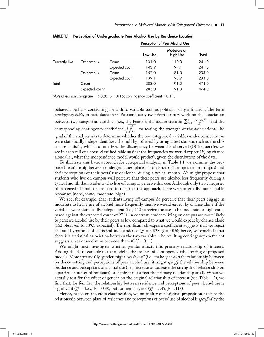
To illustrate this basic approach for categorical analysis, in Table 1.1 we examine the pro-posed relationship between undergraduates’ place of residence (off campus or on campus) and their perceptions of their peers’ use of alcohol during a typical month. We might propose that students who live on campus will perceive that their peers use alcohol less frequently during a typical month than students who live off campus perceive this use. Although only two categories of perceived alcohol use are used to illustrate the approach, there were originally four possible responses (none, some, moderate, high).
We see, for example, that students living off campus do perceive that their peers engage in moderate to heavy use of alcohol more frequently than we would expect by chance alone if the variables were statistically independent (i.e., 110 perceive the use to be moderate or high com-pared against the expected count of 97.1). In contrast, students living on campus are more likely to perceive alcohol use by their peers as low compared to what we would expect by chance alone (152 observed to 139.1 expected). The significant chi-square coefficient suggests that we reject the null hypothesis of statistical independence (χ2 = 5.828, p = .016); hence, we conclude that there is a statistical association between the two variables. The resulting contingency coefficient suggests a weak association between them (CC = 0.11).
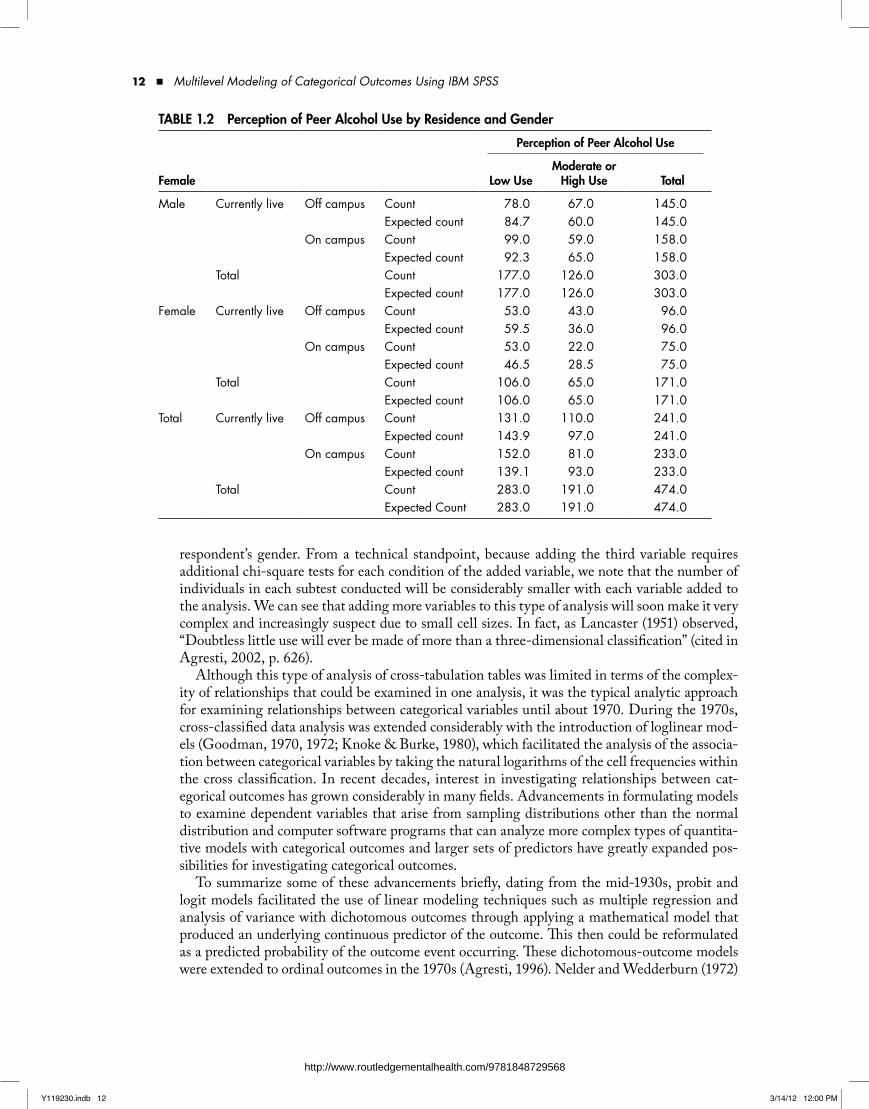
We might next investigate whether gender affects this primary relationship of interest. Adding the third variable to the model is the essence of contingency-table testing of proposed models. More specifically, gender might “wash out” (i.e., make spurious) the relationship between residence setting and perceptions of peer alcohol use; it might specify the relationship between residence and perceptions of alcohol use (i.e., increase or decrease the strength of relationship on a particular subset of residents) or it might not affect the primary relationship at all. When we actually test for the effect of gender on the original relationship of interest (see Table 1.2), we find that, for females, the relationship between residence and perceptions of peer alcohol use is significant (χ2 = 4.27, p = .039), but for men it is not (χ2 = 2.45, p = .118).
Hence, based on the cross classification, we must alter our original proposition because the relationship between place of residence and perceptions of peers’ use of alcohol is specified by the
TAble 1.1 Perception of undergraduate Peer Alcohol use by residence location
Perception of Peer Alcohol use
low useModerate or
High use Total
Currently live Off campus Count 131.0 110.0 241.0Expected count 143.9 97.1 241.0
On campus Count 152.0 81.0 233.0Expected count 139.1 93.9 233.0
Total Count 283.0 191.0 474.0Expected count 283.0 191.0 474.0
Notes: Pearson chi-square = 5.828, p = .016; contingency coefficient = 0.11.
Y119230.indb 11 3/14/12 12:00 PM
http://www.routledgementalhealth.com/9781848729568
12 ■ Multilevel Modeling of Categorical Outcomes Using IBM SPSS
respondent’s gender. From a technical standpoint, because adding the third variable requires additional chi-square tests for each condition of the added variable, we note that the number of individuals in each subtest conducted will be considerably smaller with each variable added to the analysis. We can see that adding more variables to this type of analysis will soon make it very complex and increasingly suspect due to small cell sizes. In fact, as Lancaster (1951) observed, “Doubtless little use will ever be made of more than a three-dimensional classification” (cited in Agresti, 2002, p. 626).
Although this type of analysis of cross-tabulation tables was limited in terms of the complex-ity of relationships that could be examined in one analysis, it was the typical analytic approach for examining relationships between categorical variables until about 1970. During the 1970s, cross-classified data analysis was extended considerably with the introduction of loglinear mod-els (Goodman, 1970, 1972; Knoke & Burke, 1980), which facilitated the analysis of the associa-tion between categorical variables by taking the natural logarithms of the cell frequencies within the cross classification. In recent decades, interest in investigating relationships between cat-egorical outcomes has grown considerably in many fields. Advancements in formulating models to examine dependent variables that arise from sampling distributions other than the normal distribution and computer software programs that can analyze more complex types of quantita-tive models with categorical outcomes and larger sets of predictors have greatly expanded pos-sibilities for investigating categorical outcomes.
To summarize some of these advancements briefly, dating from the mid-1930s, probit and logit models facilitated the use of linear modeling techniques such as multiple regression and analysis of variance with dichotomous outcomes through applying a mathematical model that produced an underlying continuous predictor of the outcome. This then could be reformulated as a predicted probability of the outcome event occurring. These dichotomous-outcome models were extended to ordinal outcomes in the 1970s (Agresti, 1996). Nelder and Wedderburn (1972)
TAble 1.2 Perception of Peer Alcohol use by residence and gender
Perception of Peer Alcohol use
Female low useModerate or
High use Total
Male Currently live Off campus Count 78.0 67.0 145.0Expected count 84.7 60.0 145.0
On campus Count 99.0 59.0 158.0Expected count 92.3 65.0 158.0
Total Count 177.0 126.0 303.0Expected count 177.0 126.0 303.0
Female Currently live Off campus Count 53.0 43.0 96.0Expected count 59.5 36.0 96.0
On campus Count 53.0 22.0 75.0Expected count 46.5 28.5 75.0
Total Count 106.0 65.0 171.0Expected count 106.0 65.0 171.0
Total Currently live Off campus Count 131.0 110.0 241.0Expected count 143.9 97.0 241.0
On campus Count 152.0 81.0 233.0Expected count 139.1 93.0 233.0
Total Count 283.0 191.0 474.0Expected Count 283.0 191.0 474.0
Y119230.indb 12 3/14/12 12:00 PM
http://www.routledgementalhealth.com/9781848729568
Introduction to Multilevel Models With Categorical Outcomes ■ 13
unified several of these models for examining categorical outcomes (e.g., logistic, loglinear, pro-bit models) as special cases of GLMs.
The GLM facilitates the examination of different probability distributions for the dependent variable Y using a mathematical “link” function—that is, a mathematical model that specifies the relationship between the linear predictor and the mean of the distribution function. The link function transforms the categorical outcome into an underlying continuous predictor of Y. The generalized linear model assumes that the observations are uncorrelated. Extensions of the GLM have been developed to allow for correlation between observations as occurs, for example, in repeated measures and clustered designs. More specifically, categorical models for clustered data, referred to as the GEE approach for longitudinal data (Liang & Zeger, 1986), and mixed models for logistic (e.g., Pierce & Sands, 1975) and probit (Ashford & Sowden, 1970) scales enable applications of GLM to the longitudinal and multilevel data structures typically encoun-tered with continuous and noncontinuous outcomes.
Sampling DistributionsA sampling distribution provides the probability of selecting a particular value of the variable from a population (Azen & Walker, 2011). Their properties are related to the measurement characteristics of the random outcome variable. In this instance, by “random” we mean the level of the outcome that happens by chance when drawing a sample, as related to characteristics of its underlying probability distribution. More specifically, a probability distribution is a mathemati-cal function that describes the probability of a random variable taking on particular values. Each type of outcome has a set of possible random values it can take on. For example, a continuous outcome can take on any value between a chosen interval such as 0 and 1, but a dichotomous outcome can take on only the value of 0 or 1. In this latter case, the expected value, or mean, of the outcome will simply be the proportion of times the event of interest occurs.
We assume that readers are generally familiar with multiple regression and analysis of variance (ANOVA) models for explaining variability in continuous outcomes. These techniques assume that values of the dependent variable are normally distributed about its mean with variability similar to a bell curve; that is, they result from a normal sampling distribution. There are no restrictions on the predicted values of the Level-1 outcome; that is, they can take on any real value (Raudenbush et al., 2004). As we noted previously, the residuals, or errors associated with pre-dicting Y from X at Level 1, are approximately normally distributed with a mean of 0 and some homogenous variance. In the multilevel setting, we can often transform the continuous outcome that is considerably skewed such that the residuals at Level 1 will be approximately normal.
When outcome variables are categorical, however, we have noted that different types of sam-pling distributions need to be considered at Level 1. One of the key issues is that the assumption of a normal distribution is likely to be violated. Consider the probability of flipping a coin and encountering a heads or tails. We can assume that the likelihood of encountering each pos-sibility is 1:1 (discounting any potential flaw in the coin). With a dichotomous variable, where responses are usually coded 0 and 1, there can be no normal distribution of responses around the mean. The mean is simply the proportion of “successes,” or favored events (i.e., usually coded 1), against the other event (coded 0). Over repeated trials, in the coin example, the mean will tend to be 0.5, suggesting equal heads and tails responses. Of course, in the short run, we might observe five or six heads or tails in a row. The probability of either outcome occurring is defined as the number of ways it can occur out of the total number of possible outcomes (Azen & Walker, 2011). It follows that such a random variable can assume only a finite (or countably infinite) number of values.
If we think about the probability of obtaining any particular number 1 to 6 when we roll a die, the probability for each event (or number of ways it can occur out of the total possible out-comes) is 1/6. This is an example of a discrete uniform distribution—that is, when each possible
Y119230.indb 13 3/14/12 12:00 PM
http://www.routledgementalhealth.com/9781848729568

14 ■ Multilevel Modeling of Categorical Outcomes Using IBM SPSS
outcome is equally likely to occur. The predicted probability of obtaining any number, however, cannot be less than zero or more than unity. For rolling two dice, however, when the possible combinations range from 2 to 12, we are more likely to roll a value near the mean of 7 of the distribution (e.g., perhaps 6, 7, or 8) than either a 2 or 12. Although we certainly could roll a 2 or 12 on our first trial, often we will have to roll 40 or more times before we obtain a 2 or a 12. In this latter case, the probability of either event occurring is 1/36 (1/6*1/6 = 1/36).
In Figure 1.2, we can quickly see that the total set of probabilities is not evenly distributed but, rather, is distributed in a triangular curve. For example, there are six possible combinations (6/36 = 1/6) leading to a 7 (i.e., 1,6; 2,5; 3,4; 6,1; 5,2; 4,3), but only one possible combination leading to a 2 or a 12.
With each successive die we might add, the curve of probabilities becomes more bell shaped, as suggested by the central tendency theorem. The curve would become gradually smoother than in the two-dice case, and it would appear to be closer to a bell curve, or Gaussian function. The normal distribution, therefore, implies that values near the mean will likely be encoun-tered more frequently in the population. Keep in mind, however, that a continuous distribution assigns probability 0 to every individual outcome because it can take on any real number value.
A probability distribution, therefore, is a mathematical model that links the actual out-come obtained from empirical investigation to the probability of its occurrence (Azen & Walker, 2011). If we think about a dichotomous outcome again, because the predicted value of the outcome Y can only take on two values, the random effect at Level 1 also can only be one of two values; therefore, the residuals cannot be normally distributed and no empirical data transformation can make them that way (Hox, 2010). For a dichotomous variable, this type of sampling distribution is referred to as binomial (representing the number of suc-cesses in a set of independent trials). A binomial distribution can be thought of as an experi-ment with a fixed number of independent trials, each of which can have only two possible outcomes, where, because each trial is independent, the probabilities remain constant. Our previous example of tossing a coin a number of times to determine how many times a heads occurs is an example of a binomial experiment. One commonly encountered type of binomial
02 3 4 5 6 7
Number8 9 10 11 12
1
2
Freq
uenc
y3
4
5
6
FIgure 1.2 Distribution of possible combinations of rolling two dice.
Y119230.indb 14 3/14/12 12:00 PM
http://www.routledgementalhealth.com/9781848729568
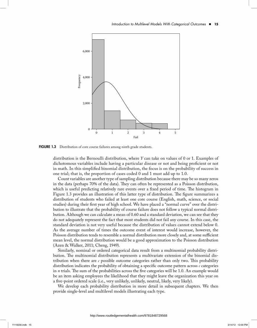
Introduction to Multilevel Models With Categorical Outcomes ■ 15
distribution is the Bernoulli distribution, where Y can take on values of 0 or 1. Examples of dichotomous variables include having a particular disease or not and being proficient or not in math. In this simplified binomial distribution, the focus is on the probability of success in one trial; that is, the proportion of cases coded 0 and 1 must add up to 1.0.
Count variables are another type of sampling distribution because there may be so many zeros in the data (perhaps 70% of the data). They can often be represented as a Poisson distribution, which is useful predicting relatively rare events over a fixed period of time. The histogram in Figure 1.3 provides an illustration of this latter type of distribution. The figure summarizes a distribution of students who failed at least one core course (English, math, science, or social studies) during their first year of high school. We have placed a “normal curve” over the distri-bution to illustrate that the probability of course failure does not follow a typical normal distri-bution. Although we can calculate a mean of 0.60 and a standard deviation, we can see that they do not adequately represent the fact that most students did not fail any course. In this case, the standard deviation is not very useful because the distribution of values cannot extend below 0. As the average number of times the outcome event of interest would increase, however, the Poisson distribution tends to resemble a normal distribution more closely and, at some sufficient mean level, the normal distribution would be a good approximation to the Poisson distribution (Azen & Walker, 2011; Cheng, 1949).
Similarly, nominal or ordered categorical data result from a multinomial probability distri-bution. The multinomial distribution represents a multivariate extension of the binomial dis-tribution when there are c possible outcome categories rather than only two. This probability distribution indicates the probability of obtaining a specific outcome pattern across c categories in n trials. The sum of the probabilities across the five categories will be 1.0. An example would be an item asking employees the likelihood that they might leave the organization this year on a five-point ordered scale (i.e., very unlikely, unlikely, neutral, likely, very likely).
We develop each probability distribution in more detail in subsequent chapters. We then provide single-level and multilevel models illustrating each type.
00 1 2 3
Fail4 5
2,000
Freq
uenc
y4,000
6,000
FIgure 1.3 Distribution of core course failures among ninth grade students.
Y119230.indb 15 3/14/12 12:00 PM
http://www.routledgementalhealth.com/9781848729568
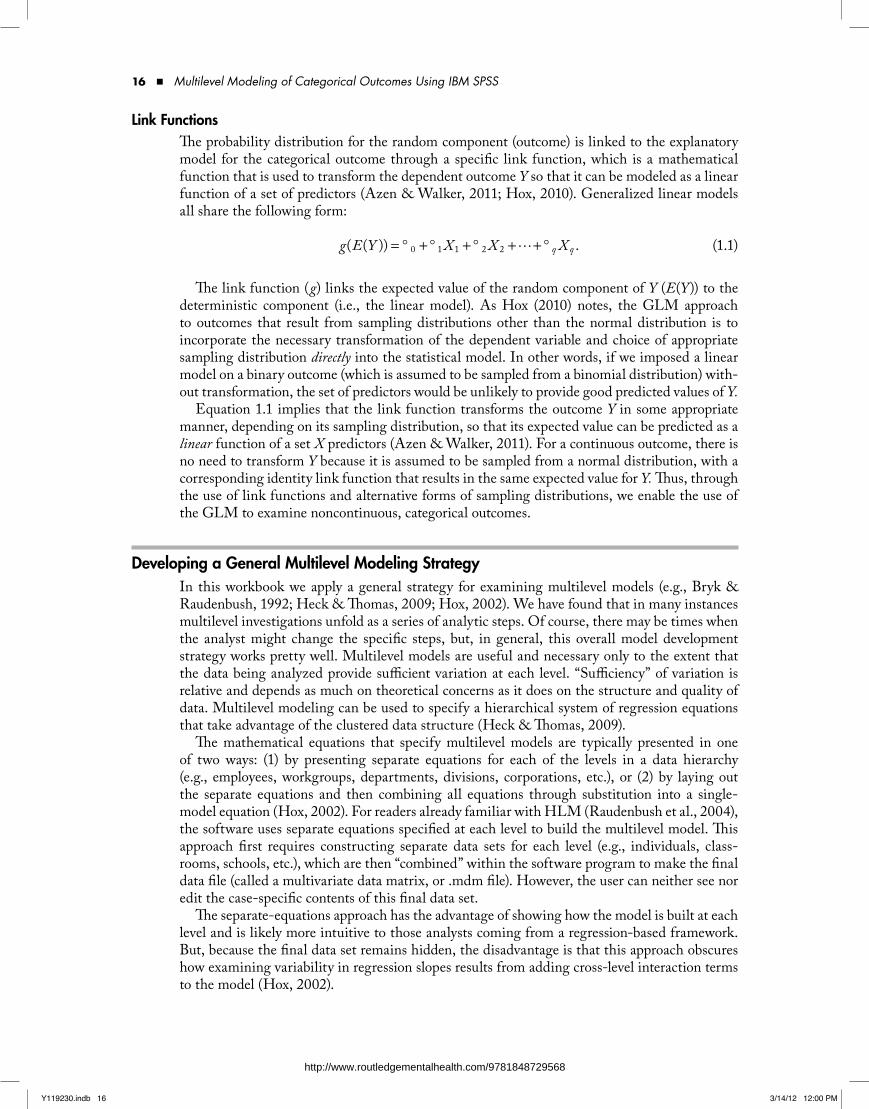
16 ■ Multilevel Modeling of Categorical Outcomes Using IBM SPSS
link FunctionsThe probability distribution for the random component (outcome) is linked to the explanatory model for the categorical outcome through a specific link function, which is a mathematical function that is used to transform the dependent outcome Y so that it can be modeled as a linear function of a set of predictors (Azen & Walker, 2011; Hox, 2010). Generalized linear models all share the following form:
= ° + ° + ° + + °g E Y X X X( ( )) .q q0 1 1 2 2 (1.1)
The link function (g) links the expected value of the random component of Y (E(Y)) to the deterministic component (i.e., the linear model). As Hox (2010) notes, the GLM approach to outcomes that result from sampling distributions other than the normal distribution is to incorporate the necessary transformation of the dependent variable and choice of appropriate sampling distribution directly into the statistical model. In other words, if we imposed a linear model on a binary outcome (which is assumed to be sampled from a binomial distribution) with-out transformation, the set of predictors would be unlikely to provide good predicted values of Y.
Equation 1.1 implies that the link function transforms the outcome Y in some appropriate manner, depending on its sampling distribution, so that its expected value can be predicted as a linear function of a set X predictors (Azen & Walker, 2011). For a continuous outcome, there is no need to transform Y because it is assumed to be sampled from a normal distribution, with a corresponding identity link function that results in the same expected value for Y. Thus, through the use of link functions and alternative forms of sampling distributions, we enable the use of the GLM to examine noncontinuous, categorical outcomes.
Developing a general Multilevel Modeling StrategyIn this workbook we apply a general strategy for examining multilevel models (e.g., Bryk & Raudenbush, 1992; Heck & Thomas, 2009; Hox, 2002). We have found that in many instances multilevel investigations unfold as a series of analytic steps. Of course, there may be times when the analyst might change the specific steps, but, in general, this overall model development strategy works pretty well. Multilevel models are useful and necessary only to the extent that the data being analyzed provide sufficient variation at each level. “Sufficiency” of variation is relative and depends as much on theoretical concerns as it does on the structure and quality of data. Multilevel modeling can be used to specify a hierarchical system of regression equations that take advantage of the clustered data structure (Heck & Thomas, 2009).
The mathematical equations that specify multilevel models are typically presented in one of two ways: (1) by presenting separate equations for each of the levels in a data hierarchy (e.g., employees, workgroups, departments, divisions, corporations, etc.), or (2) by laying out the separate equations and then combining all equations through substitution into a single-model equation (Hox, 2002). For readers already familiar with HLM (Raudenbush et al., 2004), the software uses separate equations specified at each level to build the multilevel model. This approach first requires constructing separate data sets for each level (e.g., individuals, class-rooms, schools, etc.), which are then “combined” within the software program to make the final data file (called a multivariate data matrix, or .mdm file). However, the user can neither see nor edit the case-specific contents of this final data set.
The separate-equations approach has the advantage of showing how the model is built at each level and is likely more intuitive to those analysts coming from a regression-based framework. But, because the final data set remains hidden, the disadvantage is that this approach obscures how examining variability in regression slopes results from adding cross-level interaction terms to the model (Hox, 2002).
Y119230.indb 16 3/14/12 12:00 PM
http://www.routledgementalhealth.com/9781848729568
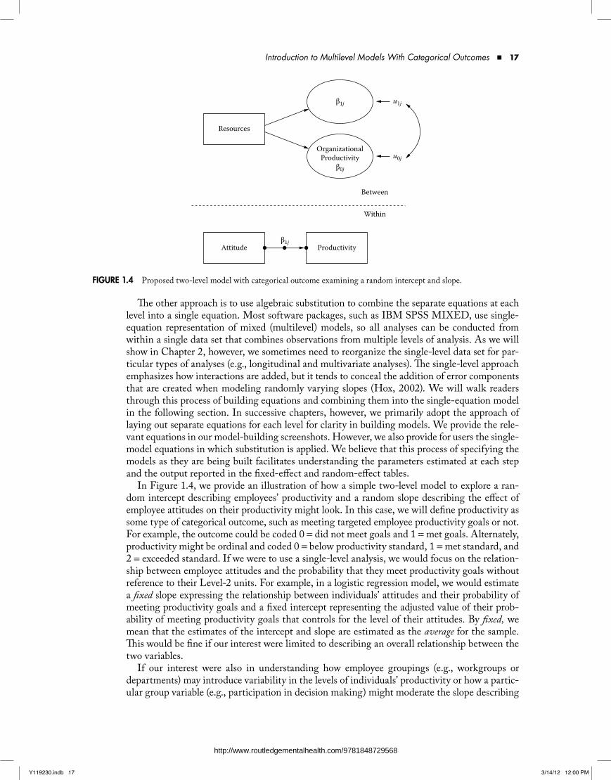
Introduction to Multilevel Models With Categorical Outcomes ■ 17
The other approach is to use algebraic substitution to combine the separate equations at each level into a single equation. Most software packages, such as IBM SPSS MIXED, use single-equation representation of mixed (multilevel) models, so all analyses can be conducted from within a single data set that combines observations from multiple levels of analysis. As we will show in Chapter 2, however, we sometimes need to reorganize the single-level data set for par-ticular types of analyses (e.g., longitudinal and multivariate analyses). The single-level approach emphasizes how interactions are added, but it tends to conceal the addition of error components that are created when modeling randomly varying slopes (Hox, 2002). We will walk readers through this process of building equations and combining them into the single-equation model in the following section. In successive chapters, however, we primarily adopt the approach of laying out separate equations for each level for clarity in building models. We provide the rele-vant equations in our model-building screenshots. However, we also provide for users the single-model equations in which substitution is applied. We believe that this process of specifying the models as they are being built facilitates understanding the parameters estimated at each step and the output reported in the fixed-effect and random-effect tables.
In Figure 1.4, we provide an illustration of how a simple two-level model to explore a ran-dom intercept describing employees’ productivity and a random slope describing the effect of employee attitudes on their productivity might look. In this case, we will define productivity as some type of categorical outcome, such as meeting targeted employee productivity goals or not. For example, the outcome could be coded 0 = did not meet goals and 1 = met goals. Alternately, productivity might be ordinal and coded 0 = below productivity standard, 1 = met standard, and 2 = exceeded standard. If we were to use a single-level analysis, we would focus on the relation-ship between employee attitudes and the probability that they meet productivity goals without reference to their Level-2 units. For example, in a logistic regression model, we would estimate a fixed slope expressing the relationship between individuals’ attitudes and their probability of meeting productivity goals and a fixed intercept representing the adjusted value of their prob-ability of meeting productivity goals that controls for the level of their attitudes. By fixed, we mean that the estimates of the intercept and slope are estimated as the average for the sample. This would be fine if our interest were limited to describing an overall relationship between the two variables.
If our interest were also in understanding how employee groupings (e.g., workgroups or departments) may introduce variability in the levels of individuals’ productivity or how a partic-ular group variable (e.g., participation in decision making) might moderate the slope describing
OrganizationalProductivity
β0j
Between
Within
Resources
β1j
β1j
u1j
Attitude Productivity
u0j
FIgure 1.4 Proposed two-level model with categorical outcome examining a random intercept and slope.
Y119230.indb 17 3/14/12 12:00 PM
http://www.routledgementalhealth.com/9781848729568
18 ■ Multilevel Modeling of Categorical Outcomes Using IBM SPSS
the effect of individuals’ attitudes on their productivity, however, we need to incorporate infor-mation about the organizational grouping of employees in our model. Once we shift into think-ing about such multilevel relationships, where employees are now nested within groups of some kind, a range of new analytical possibilities emerges. Within groups we might define a randomly varying intercept (β0j) describing the individual’s likelihood to achieve productivity targets and a randomly varying slope describing the effect of employee attitudes on the likelihood of meeting these productivity targets. The random slope (β1j) is shown in the figure with a filled dot on the line representing the relationship between attitudes and productivity. The subscript j (without i) is used to describe a randomly varying parameter at Level 2. We point out again that there is no Level-1 residual term shown in the figure. Because the probability distribution is binomial, the variance is a function of the population proportion and, therefore, cannot be estimated sepa-rately (Hox, 2010).
At the organizational level, we can formulate a model to explain variability in the random intercept and slope across organizations. First, we propose that differences in resource allocation for employee support affect the probability of meeting productivity goals (β0j) between organiza-tions. Second, we propose that differences in organizational-level resource allocation moderate the size of the effect of employee attitudes on the probability that they meet productivity goals (β1j). More specifically, we might hypothesize that organizational resource allocations consid-erably above the mean of such allocations in the sample of organizations enhance the effect of employee attitudes on their probability to attain productivity targets.
This latter type of cross-level interaction effect implies that the magnitude of a relation-ship observed within groups is dependent on contextual, structural, or process features of the groups. We therefore can formulate a Level-2 model to explain variability in intercepts and slopes (shown as ovals representing unknowns in Figure 1.2). We note that each random effect at Level 2 has its own residual variance term, which may covary (shown by the curved arrow) or not, depending on our model specification. As we have noted, this ability to examine how group processes moderate individual-level slope relationships is one of the key conceptual features of multilevel models.
In the sections that follow we offer an example of the logic we use in developing the mul-tilevel model for categorical outcomes. The core logic is consistent with the approach that we adopted in our first workbook. We elaborate that approach to accommodate the demands of the categorical models that are our focus here. We also introduce important notation conven-tions and several key features that are unique to the development of models with categorical outcomes. This is merely an introduction, as our purpose here is to reveal the broad contours in the construction and evolution of these models. This begins to set our foundation, and we pick up specific pieces of this presentation for more detailed treatment in later chapters.
Determining the Probability Distribution and link FunctionA good first step is to determine the particular sampling distribution and link function to be used in building a set of models. For generalized linear models, the choice of link function must be made initially in order to develop a model that will predict the likelihood of the outcome event of interest occurring. For some types of categorical outcomes, several choices regarding link functions can be made. Selection often hinges on several factors, such as the measurement characteristics of the outcome and its distribution in the data sample that one has available, the characteristics of the model that one is building, and the metric that one wishes to use to report the results.
As part of this initial process, it is also important that the outcome variable be defined appro-priately in terms of its scale of measurement (e.g., nominal, ordinal). For example, a correct identification of these measurement issues will generally determine the sampling distribution and link function that are specified for a particular model. Mistakenly identifying the level of measurement of dependent variables may prevent the program from processing the proposed
Y119230.indb 18 3/14/12 12:00 PM
http://www.routledgementalhealth.com/9781848729568

Introduction to Multilevel Models With Categorical Outcomes ■ 19
model or cause the user to misinterpret the output. In this case, we will assume that productiv-ity is measured as a dichotomous (nominal) variable. It will therefore have a binomial sampling distribution, and we will use a logit link function for this example. We can confirm our choices from the output in Table 1.3, which summarizes the model estimation criteria. This will be con-stant throughout the model development. We note that the output provides a caution regarding subsequent model comparison using the indices provided (because of the rescaling that takes place each time variables are added).
Developing a Null (or No Predictors) ModelOften in models with continuous outcomes, we are first interested in partitioning the variance in the outcome. We can examine the extent to which variation in a Level-1 outcome exists within Level-2 units relative to its variation between Level-2 units. Because there is no separate variance term at Level 1 for categorical variables (i.e., it is fixed to a scale factor of 1.0), it may or may not be of interest to the analyst whether to examine a model with no predictors. Hence, our primary interest may be whether there is sufficient variability in intercepts present at Level 2 (across groups) in the sample. In our example, we want to know if significant variance exists in average likelihood of individuals to meet productivity targets across groups—something that would be invisible to us in a single-level model. Little variability between the Level-2 units would suggest little need to conduct a multilevel analysis.
If we do develop such a model with no predictors, we can determine what the average prob-ability of meeting productivity goals is at the organizational level. Notice that, in Equation 1.2, we add subscripts for individuals (i) and for organizations ( j). The probability of an event occurring is generally referred to using the Greek letter pi, πij. At Level 1, the null model for individual i in organization j can be represented as follows:
η = π − π = βlog( /(1 )) ,ij ij ij j0 (1.2)
where β0j is the intercept for the jth group, and log (πij/(1 – πij)) is the mathematical function (g) that links the expected value of the dichotomous outcome Yij to the predicted values for variate ηij (McCullagh & Nelder, 1989).
In this case, as noted in Table 1.3, we chose the logit link function, which is the natural logarithm (i.e., abbreviated as log, loge, or ln) of the odds that Y = 1 (πij) versus Y = 0 (1 – πij). We could make other choices, but the logit link is most commonly used with dichotomous out-comes. We describe sampling distributions and link functions in more detail in Chapter 3. Here
TAble 1.3 Model estimation Criteria and Fit IndicesTarget Productivity
Measurement level NominalProbability distribution BinomialLink function LogitInformation criterion:
Akaike corrected 29,610.042Bayesian 29,616.831
Note: Information criteria are based on the –2 log pseudo-likelihood (29,608.041) and are used to compare models. Models with smaller information criterion values fit better. When comparing models using pseudolikelihood values, caution should be used because different data transformations may be used across the models.
Y119230.indb 19 3/14/12 12:00 PM
http://www.routledgementalhealth.com/9781848729568
20 ■ Multilevel Modeling of Categorical Outcomes Using IBM SPSS
we emphasize that the Greek letter eta (ηij) is generally used to represent the predicted values of the transformed continuous outcome (i.e., in this case, the natural logarithm of the odds Y = 1) resulting from the multiple regression equation, which in the first model only consists of the intercept. Usually, the link function used for transforming the outcome extends over the entirety of real numbers (Hox, 2010).
In a two-level model, the fixed effects are typically expressed as unstandardized β coefficients. In this case, unstandardized means that the predictor coefficients at each level are in their origi-nal metrics and indicate the change in the log odds of the underlying variate ηij (rather than the categorical outcome productivity) per unit change in the predictor (while holding any other pre-dictors in the model constant). The subscript j indicates that the intercept varies across groups. Again, there is no residual variance at Level 1 because the variance of a dichotomous outcome is tied to its mean value and, therefore, cannot be modeled separately at Level 1 (Raudenbush et al., 2004).
Between groups, variation in random intercepts (β0j) can be represented as
β = γ + u .j j0 00 0 (1.3)
Level-2 fixed-effect coefficients are generally expressed as the Greek lowercase letter gamma (γ). Variability in organizational intercepts is represented as u0j.
Through substitution, we can arrive at the corresponding single-equation model. In this case, by substituting Equation 1.3 into Equation 1.2, we arrive at the combined two-level intercept model, which can be written as
η = γ + u .ij j00 0 (1.4)
Readers should keep in mind that, in Equation 1.4 and subsequent equations in this sec-tion, ηij is the predicted log odds resulting from the regression equation linked by the logistic transformation log(π/ (1 – π)) of the odds of the outcome event occurring versus not occurring. The null model therefore provides an estimated intercept (mean) log odds of meeting employee productivity targets for all organizations. Equation 1.4 indicates there are two parameters to estimate: the intercept and the between-organization variability, or deviation, from the intercept (u0j). The estimated intercept is considered a fixed component, and the between-group variation in intercepts is considered the random effect. Information about the model’s initial parameters can be useful in examining the baseline (no predictors) model with two estimated parameters against subsequent models with more estimated parameters.
Selecting the Covariance StructureOne of the advantages of IBM SPSS MIXED is the ease in which users can specify alternative covariance structures for Level 1 and Level 2. In this case, as we noted, there is no residual component for Level 1. It is scaled to be 1.0 as the default, which provides a metric for the underlying continuous predictor ηij (Hox, 2010). The default specification is “variance com-ponents.” With only one random effect at Level 2, this is the same as specifying an identity covariance matrix or a diagonal covariance matrix. It is always useful to check the specifica-tion of the proposed model (Model 1) against the model dimension output, as summarized in Table 1.4, to make sure the model proposed is the one actually tested. The table confirms there is one fixed effect (i.e., the organization-level intercept) and one random effect (i.e., the vari-ance in intercepts across organizations at Level 2) to be estimated. “Common subjects” refers to the number of Level-2 units in the analysis (N = 122). Table 1.4 also confirms there will be one variance component (i.e., the Level-2 variance in intercepts) and no Level-1 residual vari-ance component.
Y119230.indb 20 3/14/12 12:00 PM
http://www.routledgementalhealth.com/9781848729568

Introduction to Multilevel Models With Categorical Outcomes ■ 21
Readers will note that, in the typical null model for continuous outcomes, in the single equa-tion there are three parameters to estimate, as in the following:
= ° + + εY u .ij j ij00 0 (1.5)
The two variance components from Level 1 (ε0j) and Level 2 (u0j) are used to partition the variance in an outcome into its within- and between-group components (referred to as the intra-class correlation). Because there is no separate Level-1 residual variance component (ε0j) in the multilevel GLM, the intraclass correlation (ICC), which describes the portion of variability in outcomes that lies between groups compared to the total variability, cannot be directly calcu-lated in a manner similar to multilevel models with continuous outcomes. We take this issue up further in Chapter 4.
Analyzing a level-1 Model With Fixed PredictorsAssuming that a sufficient amount of variance in Y exists at Level 2, we can investigate a model with fixed predictors at Level 1. Level-1 predictors are often referred to as X. In this case, we have one individual-level predictor (attitudes). For each individual i in organization j, a proposed model similar to Equation 1.1—in this case, summarizing the effect of employee attitudes on productivity—can be expressed as
η = β + β X ,ij j ij0 1 (1.6)
where ηij is again the predicted log odds from the logistic regression equation.Equation 1.6 suggests that, within groups, Xij (employee attitude) is related to probability of
an individual to meet productivity targets. Typically, the unstandardized within-group predic-tors (β1Xij) are either grand-mean or group-mean centered to facilitate interpretation of the coefficients. This is needed because, in multilevel models, the intercept is interpreted as the value on the outcome when all the predictors are equal to 0. Often, however, the value of 0 in its raw metric on a predictor may not be very useful in interpreting the estimates. For example, if we are examining the effect of an employee attitude (perhaps coded from 0 to 10) on productivity, there may be no individual in the sample with an attitudinal score of 0.
Grand-mean centering recenters the individual’s standing on the predictor against the mean for the predictor in the sample. For example, if the sample mean for employee attitude were 5.4, an individual on the grand mean would have her or his score rescaled to 0. An individual with a value below the mean would be rescaled to a negative number; an individual above the mean
TAble 1.4 Model 1: Covariance Parameters
Covariance ParametersResidual effect 0Random effects 1
Design Matrix ColumnsFixed effects 1Random effects 1a
Common subjects 122
Note: Common subjects are based on the subject specifications for the residual and random effects and are used to chunk the data for bet-ter performance.
a This is the number of columns per common subject.
Y119230.indb 21 3/14/12 12:00 PM
http://www.routledgementalhealth.com/9781848729568
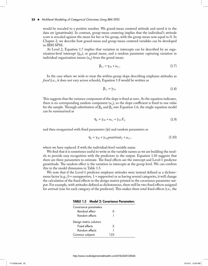
22 ■ Multilevel Modeling of Categorical Outcomes Using IBM SPSS
would be rescaled to a positive number. We grand-mean centered attitude and saved it in the data set (gmattitude). In contrast, group-mean centering implies that the individual’s attitude score is rescaled against the mean for her or his group, with the group mean now equal to 0. In Chapter 2, we describe how grand-mean and group-mean centered variables can be developed in IBM SPSS.
At Level 2, Equation 1.7 implies that variation in intercepts can be described by an orga-nization-level intercept (γ00), or grand mean, and a random parameter capturing variation in individual organization means (u0j) from the grand mean:
β = γ + u .j j0 00 0 (1.7)
In the case where we wish to treat the within-group slope describing employee attitudes as fixed (i.e., it does not vary across schools), Equation 1.8 would be written as
β = γ .j1 10 (1.8)
This suggests that the variance component of the slope is fixed at zero. As the equation indicates, there is no corresponding random component (u1j), so the slope coefficient is fixed to one value for the sample. Through substitution of β0j and β1j into Equation 1.6, the single-equation model can be summarized as
η = γ + + γu Xij j ij00 0 10 (1.9)
and then reorganized with fixed parameters (γs) and random parameters as
η = γ + γ +gmattitude u ,ij ij j00 10 0 (1.10)
where we have replaced X with the individual-level variable name.We find that it is sometimes useful to write in the variable names as we are building the mod-
els to provide easy recognition with the predictors in the output. Equation 1.10 suggests that there are three parameters to estimate. The fixed effects are the intercept and Level-1 predictor gmattitude. The random effect is the variation in intercepts at the group level. We can confirm this in the model dimension in Table 1.5.
We note that if the Level-1 predictor employee attitudes were instead defined as a dichoto-mous factor (e.g., 0 = unsupportive, 1 = supportive) or as having several categories, it will change the calculation of the fixed effects in the design matrix printed in the covariance parameter out-put. For example, with attitudes defined as dichotomous, there will be two fixed effects assigned for attitude (one for each category of the predictor). This makes three total fixed effects (i.e., the
TAble 1.5 Model 2: Covariance Parameters
Covariance parametersResidual effect 0Random effects 1
Design matrix columnsFixed effects 2Random effects 1
Common subjects 122
Y119230.indb 22 3/14/12 12:00 PM
http://www.routledgementalhealth.com/9781848729568
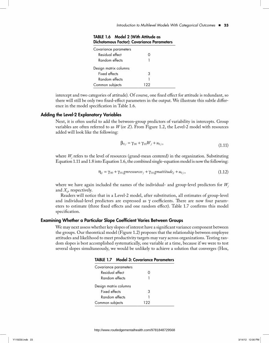
Introduction to Multilevel Models With Categorical Outcomes ■ 23
intercept and two categories of attitude). Of course, one fixed effect for attitude is redundant, so there will still be only two fixed-effect parameters in the output. We illustrate this subtle differ-ence in the model specification in Table 1.6.
Adding the level-2 explanatory VariablesNext, it is often useful to add the between-group predictors of variability in intercepts. Group variables are often referred to as W (or Z). From Figure 1.2, the Level-2 model with resources added will look like the following:
β = γ + γ +W u ,j j j0 00 01 0 (1.11)
where Wj refers to the level of resources (grand-mean centered) in the organization. Substituting Equation 1.11 and 1.8 into Equation 1.6, the combined single-equation model is now the following:
η = γ + γ + γ +gmresources gmattitude u ,ij j ij j00 01 10 0 (1.12)
where we have again included the names of the individual- and group-level predictors for Wj and Xij, respectively.
Readers will notice that in a Level-2 model, after substitution, all estimates of group-level and individual-level predictors are expressed as γ coefficients. There are now four param-eters to estimate (three fixed effects and one random effect). Table 1.7 confirms this model specification.
examining Whether a Particular Slope Coefficient Varies between groupsWe may next assess whether key slopes of interest have a significant variance component between the groups. Our theoretical model (Figure 1.2) proposes that the relationship between employee attitudes and likelihood to meet productivity targets may vary across organizations. Testing ran-dom slopes is best accomplished systematically, one variable at a time, because if we were to test several slopes simultaneously, we would be unlikely to achieve a solution that converges (Hox,
TAble 1.6 Model 2 (With Attitude as Dichotomous Factor): Covariance Parameters
Covariance parametersResidual effect 0Random effects 1
Design matrix columnsFixed effects 3Random effects 1
Common subjects 122
TAble 1.7 Model 3: Covariance Parameters
Covariance parametersResidual effect 0Random effects 1
Design matrix columnsFixed effects 3Random effects 1
Common subjects 122
Y119230.indb 23 3/14/12 12:00 PM
http://www.routledgementalhealth.com/9781848729568

24 ■ Multilevel Modeling of Categorical Outcomes Using IBM SPSS
2002). As we suggested, if the within-unit slope (e.g., gmattitude-productivity) is defined to be randomly varying across units, the Level-2 slope model can be written as
β = γ + u .j j1 10 1 (1.13)
Equation 1.13 suggests that variability in slopes can be described by a group-level average intercept coefficient (γ10), or grand mean, and a random parameter capturing variation in indi-vidual school coefficients (u1j) from the grand mean.
Through substitution, the combined single-equation model will be the following:
η = γ + γ + γ + +gmresources gmattitude u gmattitude u .ij j ij j ij j00 01 10 1 0 (1.14)
As we suggested previously, notice that the substitution of β1j in the within-group (Level 1) model (Equation 1.6) results in the addition of the interaction u1jX1ij (i.e., when X1ij is employee attitude) to the single-equation model. This interaction is considered as a random effect, which is defined as the deviation in slope for cases in group j multiplied by the Level-1 predictor score (X1) for the ith case in group j (Tabachnick, 2008). We note that when we just specify the equa-tion at Level 2 (as in Equation 1.13), the addition of the random effect as an interaction is hidden (Hox, 2010).
Covariance StructuresWith a random slope and intercept, it is often easiest first to specify a diagonal covariance struc-ture at Level 2 (using either diagonal or variance components). A diagonal covariance matrix provides an estimate of the variance for each random effect, but the covariance between the two random effects is restricted to be 0:
σ
σ
°
00
.I
S
2
2 (1.15)
There are five parameters to be estimated now. The three fixed effects to be estimated in this model are the productivity intercept, the Level-2 predictor (gmresources), and the Level-1 pre-dictor (gmattitudes). The two random effects at Level 2 are the variability in the intercept and the variability in the attitude-productivity slope. We can confirm this specification (Table 1.8).
If this model converges or reaches a solution without any warnings in the output, we can also try using a completely unstructured (Unstructured) covariance matrix of random effects. As suggested in Table 1.9, specifying an unstructured covariance matrix at Level 2 provides an additional random effect in the model, which represents the covariance between the random intercept and random slope; that is, there will be three covariance parameters
TAble 1.8 Model 4: Covariance Parameters
Covariance parametersResidual effect 0Random effects 2
Design matrix columnsFixed effects 3Random effects 2
Common subjects 122
Y119230.indb 24 3/14/12 12:00 PM
http://www.routledgementalhealth.com/9781848729568

Introduction to Multilevel Models With Categorical Outcomes ■ 25
to be estimated. We can summarize this unstructured matrix (which is a symmetric matrix) as follows:
σ σ
σ σ
°
I IS
IS S
2
2 (1.16)
The variances of the intercept and slope are in the diagonals, with their covariance as the off-diagonal element. The extra covariance parameter to be estimated is confirmed below. We note, however, that specifying an unstructured covariance matrix for random effects results in more models that fail to converge, often because the relationship between the two is nearly zero and may not vary sufficiently across units.
Adding Cross-level Interactions to explain Variation in the SlopeFinally, we would build a Level-2 model to explain variation in the Level-1 randomly vary-ing slope of interest (i.e., assuming that the slope has significant variance across groups). Our simplified model in Figure 1.4 suggests that organizational resource levels may moderate the within-unit (e.g., attitude-productivity) slope:
β = γ + γ +gmresources u .j j j1 10 11 1 (1.17)
The cross-level, fixed-effect interaction term, which combines a Level-2 predictor with the Level-1 predictor ( y11XijWj ), is built during the model specification phase in IBM SPSS. Substitution of the revised β1j model into Eq. 1.6 results in the following single-equation model:
η = γ + γ + γ + γ + +gmresources gmattitude gmresources gmattitude u gmattitude u* .ij j ij j ij j ij j00 01 10 11 1 0
(1.18)
The model represented in Equation 1.18 results in seven total parameters to estimate (i.e., if we maintain the unstructured covariance matrix at Level 2). The four fixed effects are the intercept, resources slope, employee attitudes slope, and the cross-level interaction slope (gmattitude*gmresources). The three random covariance parameters at Level 2 are again the intercept (u0j), the attitude-productivity slope (u1j), and the covariance between them. Once again, we can confirm these model specifications in the model dimension table (Table 1.10).
Selecting level-1 and level-2 Covariance StructuresOur discussion of these basic modeling steps suggests that there is considerable flexibility in defining covariance structures at Level 2. We suggest working with less complex structures first because they are more likely to converge on a solution. If there is little variance to be estimated between groups, the program will issue a warning.
TAble 1.9 Model 4a: Covariance Parameters (unstructured)
Covariance parametersResidual effect 0Random effects 3
Design matrix columnsFixed effects 3Random effects 2
Common subjects 122
Y119230.indb 25 3/14/12 12:00 PM
http://www.routledgementalhealth.com/9781848729568
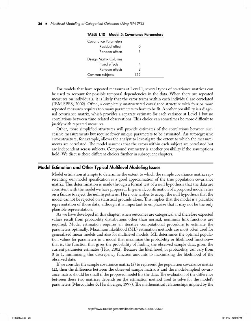
26 ■ Multilevel Modeling of Categorical Outcomes Using IBM SPSS
For models that have repeated measures at Level 1, several types of covariance matrices can be used to account for possible temporal dependencies in the data. When there are repeated measures on individuals, it is likely that the error terms within each individual are correlated (IBM SPSS, 2002). Often, a completely unstructured covariance structure with four or more repeated measures requires too many parameters to have to be fit. Another possibility is a diago-nal covariance matrix, which provides a separate estimate for each variance at Level 1 but no correlations between time-related observations. This choice can sometimes be more difficult to justify with repeated measures.
Other, more simplified structures will provide estimates of the correlations between suc-cessive measurements but require fewer unique parameters to be estimated. An autoregressive error structure, for example, allows the analyst to investigate the extent to which the measure-ments are correlated. The model assumes that the errors within each subject are correlated but are independent across subjects. Compound symmetry is another possibility if the assumptions hold. We discuss these different choices further in subsequent chapters.
Model estimation and Other Typical Multilevel Modeling IssuesModel estimation attempts to determine the extent to which the sample covariance matrix rep-resenting our model specification is a good approximation of the true population covariance matrix. This determination is made through a formal test of a null hypothesis that the data are consistent with the model we have proposed. In general, confirmation of a proposed model relies on a failure to reject the null hypothesis. Here, one wishes to accept the null hypothesis that the model cannot be rejected on statistical grounds alone. This implies that the model is a plausible representation of those data, although it is important to emphasize that it may not be the only plausible representation.
As we have developed in this chapter, when outcomes are categorical and therefore expected values result from probability distributions other than normal, nonlinear link functions are required. Model estimation requires an iterative computational procedure to estimate the parameters optimally. Maximum likelihood (ML) estimation methods are most often used for generalized linear models and also for multilevel models. ML determines the optimal popula-tion values for parameters in a model that maximize the probability or likelihood function—that is, the function that gives the probability of finding the observed sample data, given the current parameter estimates (Hox, 2002). Because the likelihood, or probability, can vary from 0 to 1, minimizing this discrepancy function amounts to maximizing the likelihood of the observed data.
If we consider the sample covariance matrix (S) to represent the population covariance matrix (Σ), then the difference between the observed sample matrix S and the model-implied covari-ance matrix should be small if the proposed model fits the data. The evaluation of the difference between these two matrices depends on the estimation method used to solve for the model’s parameters (Marcoulides & Hershberger, 1997). The mathematical relationships implied by the
TAble 1.10 Model 5: Covariance Parameters
Covariance ParametersResidual effect 0Random effects 3
Design Matrix ColumnsFixed effects 4Random effects 2
Common subjects 122
Y119230.indb 26 3/14/12 12:00 PM
http://www.routledgementalhealth.com/9781848729568

Introduction to Multilevel Models With Categorical Outcomes ■ 27
model are solved iteratively until the estimates are optimized. The difference between S and Ŝ
is described as a discrepancy function—that is, the actual difference in the two estimates based on a likelihood. The greater the difference between these two covariance matrices, the larger the discrepancy in the function becomes (Marcoulides & Hershberger, 1997).
For single-level categorical analyses, IBM SPSS GENLIN supports ML estimation using Newton-Raphson and Fisher scoring methods, which are among the most efficient and widely used estimation methods for categorical outcomes (Dobson, 1990). For multilevel models with categorical outcomes, model estimation becomes more difficult. Estimation typically relies on quasilikelihood approaches, which approximate the nonlinear functions used by a nearly linear transformation. This complicates the solving of complex nonlinear mathematical equations rep-resenting the relationships among variables in the model (Hox, 2010).
Combining multilevel data structures and GLM, therefore, can lead to much greater com-plexity in estimating model parameters and require considerably more computer time in provid-ing model estimation. The default estimation method for categorical outcomes used in GENLIN MIXED is referred to as active set method (ASM) with Newton-Raphson estimation—one well-known theoretical way to solve a constrained optimization problem that proceeds by find-ing a feasible starting point and adjusting iterative solutions until it reaches a final solution that is “optimal enough” according to a set of criteria (Nocedal & Wright, 2006).
Three-level models can be more complicated to estimate than two-level models (e.g., more cross-level interactions, changing sample sizes, etc.), but the strategy is basically the same. As we have already stated at several points, it is best to keep models simplified—for example, by including only random effects that are of strong theoretical or empirical interest. Although it is desirable to include covariances between intercepts and slopes, it is not always possible to achieve model convergence. We will address this more completely in subsequent chapters.
Determining How Well the Model FitsMaximum likelihood estimation approaches provide a number of ways to determine how well a proposed model fits, assuming that the required assumptions for producing optimal estimates hold (e.g., sufficient sample sizes, proper model specification, convergence in solving the like-lihood function is achieved). As we noted, the difference between S and S is described as a discrepancy function. ML estimation produces a model deviance statistic, which is defined as –2*log likelihood, where likelihood is the value of the likelihood function at convergence and log is the natural logarithm (Hox, 2002). This is often abbreviated as –2LL. The deviance is an indicator of how well the model fits the data. Models with lower deviance (i.e., a smaller discrep-ancy function) fit better than models with higher deviance. Nested models (i.e., when a more specific model is formed from a more general one) can be compared by examining differences in these deviance coefficients under specified conditions (e.g., changes in deviance between models per differences in degrees of freedom).
For comparing two successive single-level models, the likelihood ratio test is often used. The GENLIN output provides a likelihood ratio chi-square comparison between a current model under consideration (e.g., with one or more predictors) against an intercept-only model. Additionally, successive models can also be compared (when all of the elements of the smaller model are in the larger model) using the change in log likelihood (or the change in deviance). We can also use Akaike’s information criterion (AIC) and Bayesian information criterion (BIC) to compare competing models, where we favor models with smaller values of these indices.
Because multilevel estimation procedures with categorical outcomes are approximate only, as Hox (2010) notes, related procedures for comparisons between successive models are more tenu-ous because of the nature of the quasilikelihood estimation and the rescaling of the variance that takes place each time variables are added to a model. Because solutions are approximate, test statistics based on deviance (–2LL) are not very accurate (Hox, 2010). The GENLIN MIXED output produces an estimate of the –2 log pseudolikelihood, and we can examine the change in
Y119230.indb 27 3/14/12 12:00 PM
http://www.routledgementalhealth.com/9781848729568
28 ■ Multilevel Modeling of Categorical Outcomes Using IBM SPSS
–2 log pseudolikelihood between two successive models. However, caution should be used in interpreting this coefficient because different data transformations may be used across models.
We note also that while information criterion indices are provided (Akiake or Bayesian), they are based on the real likelihood, and Hox (2010) cautions that they may not be accu-rate when estimated with quasilikelihood estimation procedures. We can also examine indi-vidual parameters and residuals to determine where possible sources of model misfit may reside. Readers should be aware that hypothesis testing of individual parameters is typically based on a normal distribution that, with categorical variables, is based on a normal approximation. This approximation may not be optimally accurate under certain conditions, such as small sample sizes (Azen & Walker, 2011).
Syntax Versus IbM SPSS Menu Command FormulationIn MIXED, we can formulate models using either syntax statements or menu commands. We suspect that most users are more familiar with the menu framework because they have likely used that to examine single-level models (e.g., analysis of variance, multiple regression, factor analysis). We have chosen the menu-command approach for presenting our model-building procedures, but we also provide examples of syntax for each chapter in Appendix A.
In the “Statistics Display” screen, one can use the “Paste” function (within the GENLIN MIXED dialog box) to generate the underlying syntax before actually running the model. The syntax is sent to its own window within IBM SPSS and can be saved for future use. We note that with more complex models, it is often a benefit to use the syntax statements to formulate and run models for a few reasons. First, the syntax statements provide a nice record of a progres-sion of models (if the syntax files are saved and labeled according to the general modeling steps we have laid out). This is helpful if the IBM SPSS program is closed. The syntax statements provide a record of when one started and left off in building a series of models. This saves time when working with dozens of models over an extended period of time.
Second, we find that pasting the syntax is a good way to check whether the model we are running actually corresponds with the model that we had in mind. Often, doing this helps us see where we have forgotten or incorrectly specified something. This becomes more important when the multilevel models being investigated take a considerable amount of time to produce a solution. We have also found that it is easier to reorganize the syntax statements than to rebuild the whole model from the menu commands if we wish to change the order of the variables in our output tables. Generally, we like to present the output such that the predictors explaining intercepts are organized by levels of the data hierarchy and the predictors that explain variation in a random slope (i.e., cross-level interactions) are similarly organized. This helps readers see that there are two separate components (i.e., the intercept model and the slope model). Using the syntax statements also saves time if we just wish to change the specification of a covariance matrix or include (or exclude) a particular random or fixed effect.
Third, we recommend caution in reflexively adopting the IBM SPSS defaults, as these will sometimes introduce problematic conditions on the models being estimated. We find that print-ing the syntax statements can help alert analysts to the underlying defaults embedded in the model-building procedures, as well as one’s choices to override default settings. Regardless of the type of model being developed, it is always good practice to review these default settings to ensure that they are appropriate for one’s purposes.
Sample SizeUnder various sampling conditions (e.g., how individuals and units were selected, numbers selected, missing or incomplete responses), there has been considerable debate among method-ologists about the efficiency of ML estimation (Goldstein, 1995; Longford, 1993; Morris, 1995). An important conceptual distinction between single-level and multilevel analyses is that sample size considerations are quite different. Multilevel modeling requires sufficient sample size at each
Y119230.indb 28 3/14/12 12:00 PM
http://www.routledgementalhealth.com/9781848729568

Introduction to Multilevel Models With Categorical Outcomes ■ 29
level of analysis for optimal estimation. In smaller group samples, typical ML-based estimation may result in a downward bias in the estimation of variance components and standard errors. As we have noted, multilevel modeling of categorical outcomes creates more complex estima-tion due to the nature of their scales of measurement and the resulting need to use approximate estimation methods (e.g., quasilikelihood). Under certain types of sample conditions (e.g., small samples, several hierarchical levels) and model specification, estimation may become much more challenging. When the estimation does not lead to an acceptable solution (e.g., being able to estimate a variance component), a warning message is issued as part of the output. In other cases, the model may stop estimating and issue a message that an “internal error” has stopped the model estimation process.
It is important to keep in mind that under less than ideal sampling conditions (e.g., small numbers of groups, convenience samples), it may be difficult to determine whether model results might be replicated in other samples. When only a limited number of groups is available, users can apply the Satterthwaite correction to the calculation of standard errors; this provides more conservative (i.e., larger) estimates of standard errors (Loh, 1987). We note that it is often more efficient to add higher level units than to add individuals within groups because this former approach generally reduces the need for sizable samples within the groups and tends to be more efficient in estimating random coefficients.
PowerPower refers to the ability to detect an effect if one exists. In the single-level analysis, most researchers know that the significance level (α), the effect size (i.e., with larger effects easier to detect), and the sample size are determinants of power. Multilevel models raise a number of additional issues involving power. Issues about power typically concern the appropriate (or mini-mum) sample size needed for various types of multilevel analyses (e.g., determining whether an intercept or slope varies across groups). As we suggested previously, one issue refers to the sample size required to ensure that estimates of fixed effects (e.g., at Level 1 and Level 2) and variances are unbiased (i.e., sampling bias). In most multilevel studies, the estimation of Level-2 effects is generally of greater concern because the number of groups available may be limited. Adding groups (as opposed to individuals) will tend to reduce parameter bias at that level. As Snijders (2005) shows, when fixed effects are the focus, characteristics of the groups themselves have little bearing on the precision of Level-1 estimates.
Another issue refers to the minimum sample size required to ensure that an effect would be detected if, in fact, one existed (i.e., power). In addition to these two determinants of power, in multilevel analyses at least two other considerations inform estimates of power: sample size at each level (i.e., the number of individuals i within each group j and the number of j groups) and the intraclass correlation (see Muthén & Satorra, 1995, for further discussion). With larger intraclass correlations, the power to detect Level-1 effects will be lower (because the groups are more homogeneous), holding sample size constant at all levels. This suggests that the power to detect Level-2 effects is much more sensitive to the number of groups in the sample as opposed to the number of observations within groups.
As designs become more complex, the need for larger samples at both levels increases. For example, in a given sample of individuals within groups, slopes in some units may be less reli-ably estimated than intercepts because, although intercepts depend only on the average level (mean) of a variable within each group, slope estimates depend on the levels of an outcome and a particular covariate, as well as the variability of their covariance among individuals within each group (Mehta & Neale, 2005). This means that estimating variability in random slopes across units generally requires larger sample sizes for more stable estimates than simply estimating random intercepts.
Complications can also arise due to correlations between random effects and the investigation of cross-level interactions (Raudenbush & Bryk, 2002), as well as the challenges of estimating
Y119230.indb 29 3/14/12 12:00 PM
http://www.routledgementalhealth.com/9781848729568
30 ■ Multilevel Modeling of Categorical Outcomes Using IBM SPSS
models with categorical outcomes and complex sets of relationships that we noted previously. As this limited discussion of power suggests, a number of considerations must take place to assess potential bias in parameter estimates and power in various types of multilevel designs. See Snijders and Bosker (1999) or Heck and Thomas (2009) for further discussion of issues related to power.
Missing DataUsers should consider data preparation and data analysis as two separate steps. Missing data can be a problem in multilevel applications, depending upon the extent to which the data are missing and whether or not the data are missing at random. In some modeling situations, there may be considerable missing data. It is often useful to determine the amount of missing data as a first step in a data analysis, as well as the number of missing data patterns. A number of strategies for dealing with missing data are available. Some traditional approaches (e.g., listwise or pairwise deletion, mean substitution, simple imputation, weighting) lead to biased results in various situations (Peugh & Enders, 2004; Raykov & Marcoulides, 2008). It helps to know the defaults for software programs.
Traditionally, the typical way of handling missing data was to use listwise (i.e., eliminat-ing any case with at least one missing value) or pairwise (i.e., eliminating pairs of cases when missing data are present, as in calculating a correlation) deletion, mean substitution, or vari-ous regression-based approaches (e.g., estimating outcomes with dummy-coded missing data flags to determine whether there were differences in outcomes associated with individuals with missing versus complete data). Generally, listwise, pairwise, mean substitution, and various regression-based approaches are not considered acceptable solutions because they lead to biased parameter estimation. For example, listwise deletion is only valid when the data are missing completely at random (e.g., as when selecting a random sample from a population), which is sel-dom the case using real data. Acceptable solutions include multiple imputation (MI) of plausible values and FIML estimation in the presence of missing data (Peugh & Enders, 2004; Raykov & Marcoulides, 2008).
Handling missing data in an appropriate manner depends on one’s knowledge of the data set and why particular values may be missing. In general, there are three main types of missing data (see Raykov & Marcoulides, 2008, for further discussion). These include data that are missing completely at random (MCAR), missing at random (MAR), and nonignorable missing (NIM) data. For data to be MCAR, strong assumptions must hold (Raykov & Marcoulides, 2008). The missing data on a given outcome should be unrelated to a subject’s standing on the outcome or to other observed data or unobserved (missing) data in the analysis. Typically, this assumption is only met when the data are missing by design, as in the situation where we draw a random sample of the studied population.
For example, we could generate a sample with, say, 25% data missing on an outcome such as student math proficiency scores. If the probability of data being missing on the outcome is related to missing data on a covariate, but not to subjects’ standing on the outcome (e.g., if stu-dents who have missing data on attendance do not have a greater probability to have missing data on math proficiency outcomes), then the data are MAR (Raykov & Marcoulides, 2008). If the probability of missing on the outcome is related to standing on the outcome, even for individuals with the same value on a covariate (e.g., there are more missing low-math data than missing average- and high-math data among students with the same attendance level), the data are NIM. This latter type of missing data can produce more bias on model estimation than either of the other situations because the missing data on achievement are related to actual values of individual achievement for those subjects who do not take the test.
We note that, as an analytic routine, the MIXED program is limited in its ability to deal with missing data. As a default, the program uses listwise deletion of cases when data are miss-ing. This means that any individual with data missing on any variable will be dropped from the
Y119230.indb 30 3/14/12 12:00 PM
http://www.routledgementalhealth.com/9781848729568

Introduction to Multilevel Models With Categorical Outcomes ■ 31
analysis. This can result in a tremendous loss of data and biased parameter estimation. IBM SPSS does provide a number of options for examining missing data in addition to listwise, pairwise, or mean substitution. For example, the Statistics Base program includes a basic pro-gram to replace missing values. This is, however, a limited routine that provides the following replacement methods: series mean, mean of nearby points, median of nearby points, linear inter-polation, and linear trend at point. It is accessed from the program’s toolbar, where the user can select TRANSFORM and REPLACE MISSING VALUES.
IBM SPSS also has a missing-data module that can provide multiple imputation for missing data, but it must be purchased as an add-on program. This allows the user to generate a num-ber of data sets with random values imputed for missing values. Students using the IBM SPSS Graduate Pack may have to upgrade to a regular version of the IBM SPSS Statistics Base and Advanced Statistics software in order to add on the missing data module to use prior to IBM SPSS MIXED. Using this add-on module, patterns of missing data can first be identified and then plausible values can be imputed using the EM (expectation maximization) algorithm.
Expectation maximization is a common method for obtaining ML estimates with incom-plete data that has been shown to reduce bias due to missing data (Peugh & Enders, 2004). In this approach, the model parameters are viewed as missing values to be estimated. Obtaining estimates involves an iterative, two-step process where missing values are first imputed and then a covariance matrix and mean vector are estimated. This repeats until the difference between covariance matrices from adjacent iterations differs by a trivial amount (see Peugh & Enders, 2004, for further discussion). The process can be used to create a number of imputed data sets, where each simulates a random draw from the distribution of plausible values for the missing data (Peugh & Enders, 2004). These can be saved as separate data sets and then analyzed. One of the advantages of this approach is that other variables can also be used to supply information about missing data, but they need not be included in the actual model estimation. This approach to missing data is recommended when the assumption that the data are MAR is plausible.
For multilevel data, we note that at present IBM SPSS does not generally support FIML estimation in the presence of observations that may be MCAR or MAR, as is found in some software programs (Raykov & Marcoulides, 2008). What this means is that the cases are simply dropped from the analysis. In contrast, however, when the data are vertically arranged (e.g., when a single individual may have several observations or rows representing different time peri-ods), only that particular occasion will be dropped if there is a missing value present. So, for example, if there are four observations per individual (e.g., four successive math scores) and one observation is missing for a particular individual, the other three observations would be used in calculating that individual’s growth over time. This will typically yield unbiased estimates if data are MAR (Raykov & Marcoulides, 2008).
In Table 1.11 we summarize a simple logistic regression model to estimate the effects of gender and socioeconomic status on likelihood to be proficient in reading based on 20 individuals with
TAble 1.11 log Odds estimates (N = 20)95% Wald
confidence interval Hypothesis test
Parameter B Std. error lower upper Wald χ2 df Sig.
(Intercept) 1.892 1.1090 –0.282 4.065 2.910 1 0.088Female –0.564 1.2336 –2.981 1.854 0.209 1 0.648Zses 1.945 0.9478 0.087 3.802 4.210 1 0.040(Scale) 1a
Notes: Dependent variable: readprof; model: (intercept), female, Zses.a Fixed at the displayed value.
Y119230.indb 31 3/14/12 12:00 PM
http://www.routledgementalhealth.com/9781848729568
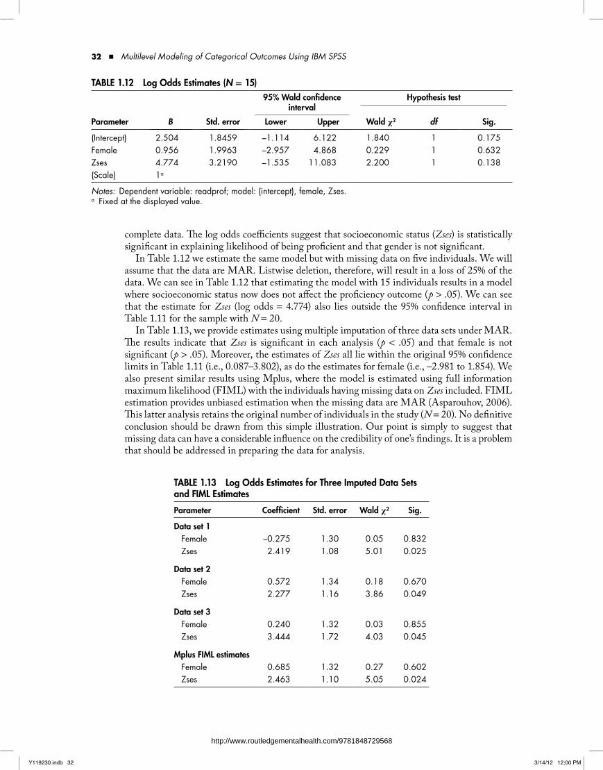
32 ■ Multilevel Modeling of Categorical Outcomes Using IBM SPSS
complete data. The log odds coefficients suggest that socioeconomic status (Zses) is statistically significant in explaining likelihood of being proficient and that gender is not significant.
In Table 1.12 we estimate the same model but with missing data on five individuals. We will assume that the data are MAR. Listwise deletion, therefore, will result in a loss of 25% of the data. We can see in Table 1.12 that estimating the model with 15 individuals results in a model where socioeconomic status now does not affect the proficiency outcome (p > .05). We can see that the estimate for Zses (log odds = 4.774) also lies outside the 95% confidence interval in Table 1.11 for the sample with N = 20.
In Table 1.13, we provide estimates using multiple imputation of three data sets under MAR. The results indicate that Zses is significant in each analysis (p < .05) and that female is not significant (p > .05). Moreover, the estimates of Zses all lie within the original 95% confidence limits in Table 1.11 (i.e., 0.087–3.802), as do the estimates for female (i.e., –2.981 to 1.854). We also present similar results using Mplus, where the model is estimated using full information maximum likelihood (FIML) with the individuals having missing data on Zses included. FIML estimation provides unbiased estimation when the missing data are MAR (Asparouhov, 2006). This latter analysis retains the original number of individuals in the study (N = 20). No definitive conclusion should be drawn from this simple illustration. Our point is simply to suggest that missing data can have a considerable influence on the credibility of one’s findings. It is a problem that should be addressed in preparing the data for analysis.
TAble 1.12 log Odds estimates (N = 15)95% Wald confidence
intervalHypothesis test
Parameter B Std. error lower upper Wald χ2 df Sig.
(Intercept) 2.504 1.8459 –1.114 6.122 1.840 1 0.175Female 0.956 1.9963 –2.957 4.868 0.229 1 0.632Zses 4.774 3.2190 –1.535 11.083 2.200 1 0.138(Scale) 1a
Notes: Dependent variable: readprof; model: (intercept), female, Zses.a Fixed at the displayed value.
TAble 1.13 log Odds estimates for Three Imputed Data Sets and FIMl estimates
Parameter Coefficient Std. error Wald χ2 Sig.
Data set 1Female –0.275 1.30 0.05 0.832Zses 2.419 1.08 5.01 0.025
Data set 2Female 0.572 1.34 0.18 0.670Zses 2.277 1.16 3.86 0.049
Data set 3Female 0.240 1.32 0.03 0.855Zses 3.444 1.72 4.03 0.045
Mplus FIMl estimatesFemale 0.685 1.32 0.27 0.602Zses 2.463 1.10 5.05 0.024
Y119230.indb 32 3/14/12 12:00 PM
http://www.routledgementalhealth.com/9781848729568
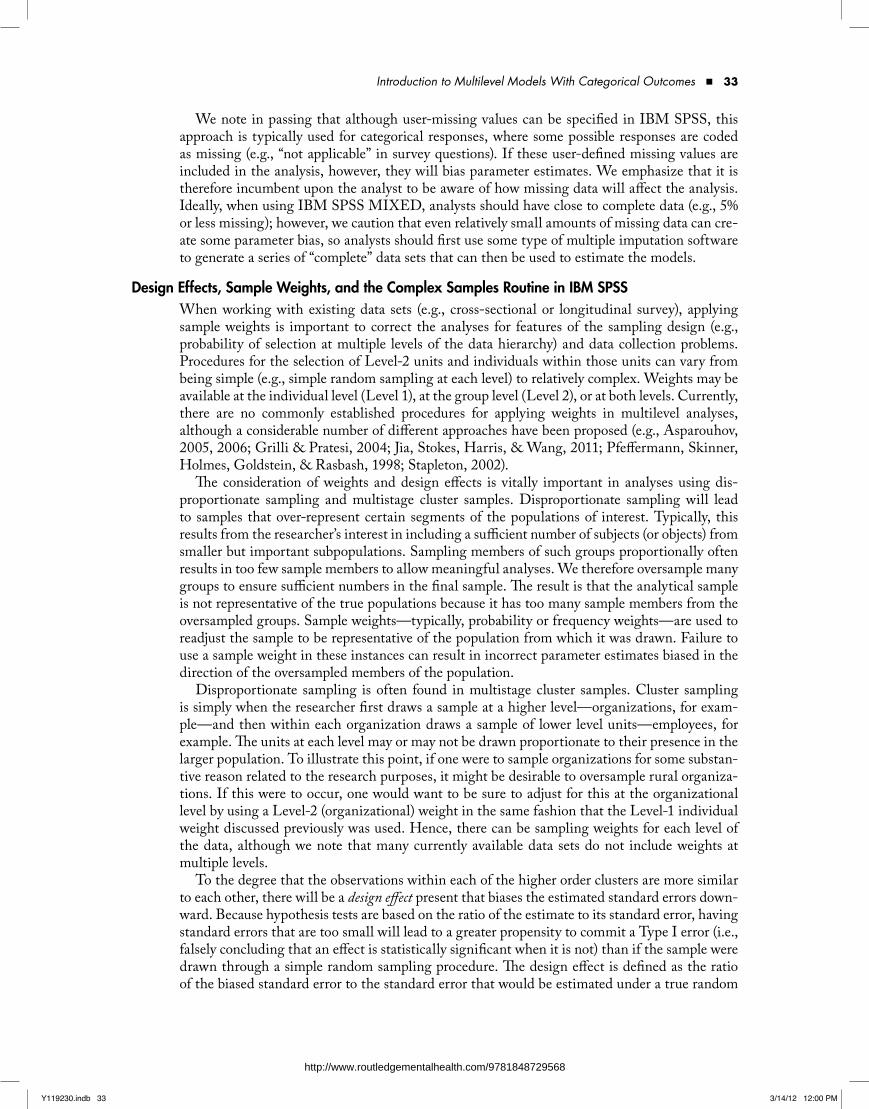
Introduction to Multilevel Models With Categorical Outcomes ■ 33
We note in passing that although user-missing values can be specified in IBM SPSS, this approach is typically used for categorical responses, where some possible responses are coded as missing (e.g., “not applicable” in survey questions). If these user-defined missing values are included in the analysis, however, they will bias parameter estimates. We emphasize that it is therefore incumbent upon the analyst to be aware of how missing data will affect the analysis. Ideally, when using IBM SPSS MIXED, analysts should have close to complete data (e.g., 5% or less missing); however, we caution that even relatively small amounts of missing data can cre-ate some parameter bias, so analysts should first use some type of multiple imputation software to generate a series of “complete” data sets that can then be used to estimate the models.
Design effects, Sample Weights, and the Complex Samples routine in IbM SPSSWhen working with existing data sets (e.g., cross-sectional or longitudinal survey), applying sample weights is important to correct the analyses for features of the sampling design (e.g., probability of selection at multiple levels of the data hierarchy) and data collection problems. Procedures for the selection of Level-2 units and individuals within those units can vary from being simple (e.g., simple random sampling at each level) to relatively complex. Weights may be available at the individual level (Level 1), at the group level (Level 2), or at both levels. Currently, there are no commonly established procedures for applying weights in multilevel analyses, although a considerable number of different approaches have been proposed (e.g., Asparouhov, 2005, 2006; Grilli & Pratesi, 2004; Jia, Stokes, Harris, & Wang, 2011; Pfeffermann, Skinner, Holmes, Goldstein, & Rasbash, 1998; Stapleton, 2002).
The consideration of weights and design effects is vitally important in analyses using dis-proportionate sampling and multistage cluster samples. Disproportionate sampling will lead to samples that over-represent certain segments of the populations of interest. Typically, this results from the researcher’s interest in including a sufficient number of subjects (or objects) from smaller but important subpopulations. Sampling members of such groups proportionally often results in too few sample members to allow meaningful analyses. We therefore oversample many groups to ensure sufficient numbers in the final sample. The result is that the analytical sample is not representative of the true populations because it has too many sample members from the oversampled groups. Sample weights—typically, probability or frequency weights—are used to readjust the sample to be representative of the population from which it was drawn. Failure to use a sample weight in these instances can result in incorrect parameter estimates biased in the direction of the oversampled members of the population.
Disproportionate sampling is often found in multistage cluster samples. Cluster sampling is simply when the researcher first draws a sample at a higher level—organizations, for exam-ple—and then within each organization draws a sample of lower level units—employees, for example. The units at each level may or may not be drawn proportionate to their presence in the larger population. To illustrate this point, if one were to sample organizations for some substan-tive reason related to the research purposes, it might be desirable to oversample rural organiza-tions. If this were to occur, one would want to be sure to adjust for this at the organizational level by using a Level-2 (organizational) weight in the same fashion that the Level-1 individual weight discussed previously was used. Hence, there can be sampling weights for each level of the data, although we note that many currently available data sets do not include weights at multiple levels.
To the degree that the observations within each of the higher order clusters are more similar to each other, there will be a design effect present that biases the estimated standard errors down-ward. Because hypothesis tests are based on the ratio of the estimate to its standard error, having standard errors that are too small will lead to a greater propensity to commit a Type I error (i.e., falsely concluding that an effect is statistically significant when it is not) than if the sample were drawn through a simple random sampling procedure. The design effect is defined as the ratio of the biased standard error to the standard error that would be estimated under a true random
Y119230.indb 33 3/14/12 12:00 PM
http://www.routledgementalhealth.com/9781848729568

34 ■ Multilevel Modeling of Categorical Outcomes Using IBM SPSS
sample design. So, for example, if we know that the true standard error was 1.5, but the biased standard error estimated from the data collected through the multistage cluster sample was 1.2, the calculated design effect would be 1.5/1.2 = 1.25.
One standard measure of this within-unit (dis)similarity is the intraclass correlation, or ICC—the proportion of total variance in the outcome due to within-unit differences at higher levels. The higher the ICC is, the larger will be the design effect. Hox (2010) notes that the ICC can be viewed as another way to think about the degree of correlation within clusters. An ICC of .165, which suggests that 16.5% of the variance in the individual-level outcome exists between clusters, could also be viewed as an indication that one might expect a within-cluster correlation of .165 between individuals.
This conceptual connection between the ICC and within-cluster correlation is important in understanding design effects. In short, the greater the between-cluster variance in the individ-ual-level outcome is, the more homogenous will be the individual observations within each of the clusters. To the extent that there exist within-cluster similarities, estimates of the Level-1 variances will be smaller than they would be if the sample were collected through a simple random sample design (where such clustering would be irrelevant to the variance structure). The implication central to our interests is that ignoring the clustering that is part of the sample design will yield downwardly biased estimates of the standard error.
The last several versions of SPSS have made available a COMPLEX SAMPLES module (as an add-on) that allows the user to incorporate design information into the model to adjust for the design effects described previously. This module produces results for single-level models incorporating design information and sample weights. As such, the parameter estimates are adjusted for both disproportionate sampling and cluster sampling. In the single-level context, this is the appropriate way to analyze data collected through complex sample designs. In this type of approach, similarities among individuals due to clustering are treated as “noise” that is adjusted out of the analysis, rather than as the focus of the analysis.
Multilevel models, by design, capitalize on the clustered nature of data, and it is quite com-mon to see these models used with large-scale survey data that have been collected through complex sample designs. The same cautions outlined previously apply to estimates produced using various forms of multilevel models. Although multilevel models capitalize on the clustered nature of the data, they do nothing to address disproportionate sampling and, without proper weighting, they will produce incorrect parameter estimates. Sample weights are often essential to generate accurate estimates.
Weighting for unequal selection is relatively well established for single-level analysis. The COMPLEX SAMPLE module allows adjustments to be made for sample design effects (which can include clustering) but maintains a single-level analysis after adjustment for features of the sampling scheme. In this type of approach, similarities among individuals due to clustering are treated as unwanted variance that is adjusted out of the analysis. We are unaware of any docu-mentation that specifically discusses multilevel models as complex sampling models within IBM SPSS. A standard two-level model would be an example of a two-stage cluster sampling design.
In contrast to weighting in single-level analyses, developing weighted analyses in the multi-level context presents a number of more complicated challenges and limitations. Research in this area is ongoing, and important advances have been made over the last 10 years. Most multilevel software programs now include one or more weighting options. Several programs with which we are familiar (HLM 7, LISREL 8.8, Mplus 6.1) incorporate design weights that combine information on clustering, the degree of intraclass correlation, and disproportionate sampling to create a set of scaled weights that will produce accurate estimates at each level of analysis. IBM SPSS allows for the incorporation of simple sample weights (an approximate frequency weight) in the MIXED and GENLIN MIXED routines; however, the current version does not enable a scaling adjustment that accommodates the effects of clustering in the sample design. We believe this is an important limitation of the IBM SPSS program.
Y119230.indb 34 3/14/12 12:00 PM
http://www.routledgementalhealth.com/9781848729568
Introduction to Multilevel Models With Categorical Outcomes ■ 35
A number of factors can influence the estimation of model parameters. These factors include the method of scaling the weights at Level 1 (i.e., how weights are scaled within the clusters), the size of the clusters, the relative invariance of the selection method applied to clusters (referred to as “informativeness”), the presence of missing data, and the intraclass correlation (Asparouhov, 2006). The scaling of Level-1 sample weights is very important in the multilevel context, helping to improve efficiency and decrease bias in estimation (Pfefferman et al., 1998; Skinner, 2005). Asparouhov explains that the scaling of the weights at Level 1 involves multiplying the weights by a scaling constant so that the sum of the weights is equal to some kind of characteristic of the cluster (e.g., cluster size).
Although many of the software programs used for estimating multilevel models enable the appropriate scaling, IBM SPSS does not yet include this feature. If sample weighting is essential to the analysis, it may be better to use another of the available programs or to revert to a single-level formulation within SPSS through its COMPLEX SAMPLES module. More specifically, as Aspouhuov (2006) suggests, if sampling weights present in a secondary data set are designed for a single-level analysis, it may be best to stick with that type of design and conduct a single-level analysis designed for stratified and cluster sampling designs.
Aspouhuov (2006) provides two contrasting situations illustrating this point. First, he notes that when weights are only present at Level 2 (i.e., where clusters have been sampled with unequal probability), we can identify this situation as within the framework of single-level weighted modeling, and methods available for single-level weighted analysis can be applied with consistent estimations regardless of the size of the clusters. Although the model is multilevel, the nature of the weighting is not. Of course, if sample weights are also provided at Level 1, this will change. Second, he suggests that the situation is different when weights are only provided at Level 1, as the unequal probability of selection is applied to dependent units and, therefore, the assumptions of the single-level method of analysis will be violated. The bottom line is that if the single-level sample weights cannot be properly scaled to the multilevel context, it may be better to use a single-level analysis. This threat may be more severe when estimating models with categorical outcomes (Rabe-Hesketh & Skrondal, 2006).
An exampleWe provide one simple example of a comparison between results we obtained with Mplus and HLM, which have Level-1 and Level-2 weights available for multilevel analysis, and the single-level weighted analysis available in IBM SPSS. In the example, there are 5,952 individuals nested in 185 units with a dichotomous outcome. For HLM, Level-1 weights were scaled within Level-2 units such that the sum of these weights equals the size of the respective Level-2 unit (Raudenbush et al., 2004). For Mplus, we scaled Level-1 weights so that they also summed to the cluster sample size.
In Table 1.14, we first provide unweighted estimates for the within- and between-group vari-ables using SPSS (i.e., SPSS UN). We next provide the HLM estimates with sample weights included at Levels 1 and 2. Third, we provide the SPSS estimates using only the Level-1 weights (SPSS L1W), and then we provide the SPSS estimates using only Level-2 weights (SPSS L2W). Finally, we also provide the Mplus estimates for the within-groups portion of the model only (i.e., Mplus Level-2 estimates are not log odds coefficients).
We note that the unweighted estimates differ considerably on most variables from the other estimates at both levels. First, there are more findings of significance at Level 2 than for the HLM results (i.e., five versus four, respectively). The Level-1 estimates also seem a bit too large for a couple of the variables. Second, applying only the Level-1 weights in SPSS also results in five significant parameters at Level 2. Third, when we apply only the Level-2 weights in SPSS, the pattern of the Level-2 results is consistent with HLM (but the size of the coefficients differs in some cases), and the estimated Level-1 coefficients and significance levels are consistent with HLM and Mplus. In this model, however, the significance levels of all effects are based on the
Y119230.indb 35 3/14/12 12:00 PM
http://www.routledgementalhealth.com/9781848729568

36 ■ Multilevel Modeling of Categorical Outcomes Using IBM SPSS
number of Level-2 units rather than on the number of individuals in the sample. Finally, Mplus and HLM provide consistent estimates at Level 1, as we might expect.
No definitive conclusions should be drawn from this one example data set. We provide these results only to make the point that using sample weights (and using them correctly) does make a difference in the accuracy of the estimates obtained. We are hopeful that the application of multilevel sampling weights will be included in future versions of the software. In the interim, we call attention to recent work by Chantala, Blanchette, and Suchindran (2011) providing SAS and Stata routines to generate scaled weights that could be imported into other multilevel software programs (such as IBM SPSS).
Differences between Multilevel Software ProgramsIn preparing this handbook, we compared categorical models estimated using IBM SPSS with models estimated using other multilevel software with which we are familiar (e.g., HLM, Mplus). Different software programs use slightly different algorithms to estimate models—for example, in calculating standard errors, especially in small groups. There are also differences in the means of testing the variance components. For example, IBM SPSS uses a Wald z-test, and HLM uses a chi-square test. In general, however, we have found that the differences in software are generally small; that is, output will carry the same substantive interpretation. We provide a couple of examples in Appendix B.
As we noted in the previous section, HLM and Mplus currently have procedures available for applying sample weights at two levels, but IBM SPSS does not yet have this capability. However, it has taken a number of years for these other two programs to incorporate sample weights at two levels into their analytic routines. The MIXED routine is still relatively new as a multilevel analytic program. We find that it is very compatible with well-established programs in almost every other way (and it exceeds them in some other ways).
TAble 1.14 Fixed-effect estimates for unweighted and Weighted Analyses
SPSS(uN) HlM SPSS (l1W) SPSS (l2W) MPluSa
SchoolIntercept –2.26d –2.41d –2.22d –2.26d
sSES 1.18d 1.21d 1.29d 1.32d
Private –0.28b –0.30 –0.29b –0.35General 0.49d 0.47b 0.44c 0.43b
RankMath 0.01d 0.00b 0.00 d 0.00b
City 0.17 0.27 0.14 0.28Large City 0.08 0.19 0.12 0.13
IndividualSES 0.25d 0.19b 0.24d 0.19b 0.20b
Math –0.00d –0.00d –0.00d –0.00d –0.00d
Female –0.24c –0.23b –0.22c –0.22b –0.23b
Interaction 0.56d 0.52c 0.54d 0.50c 0.51c
a Mplus between-group estimates are not in a log odds metric.b p < .05.c p < .01.d p < .001.
Y119230.indb 36 3/14/12 12:00 PM
http://www.routledgementalhealth.com/9781848729568

Introduction to Multilevel Models With Categorical Outcomes ■ 37
SummaryIn this chapter, we have developed a context and rationale for the use of multilevel models in the social and behavioral sciences. The use of multilevel analysis can add substantive information about how processes unfold at various levels of a data hierarchy. We suggested that multilevel techniques support the specification of more complex theoretical relationships than is possible using tradi-tional single-level regression analyses. Analytical approaches that can be used to model complex relationships have greatly expanded over the past couple of decades, and these analytical alterna-tives allow us to investigate social processes in more theoretically and methodologically appropri-ate ways. Substantive progress in a field is often achieved when headway occurs simultaneously on conceptual and methodological fronts. In the next chapter, we take care of a bit of housekeeping by providing an overview of some important data management techniques. Arranging the data for analysis in IBM SPSS is fairly straightforward. We provide the reader with a few essential steps necessary to put data sets in proper order for analysis using IBM SPSS MIXED.
Y119230.indb 37 3/14/12 12:00 PM
http://www.routledgementalhealth.com/9781848729568


