Multimodal magnetic resonance imaging at 3 T and...

POLITECNICO DI MILANO

Research Doctorate Course in Bioengineering

XXVII Cycle

Final dissertation

Multimodal magnetic resonance imaging at 3 T and

challenges for application at ultra-high field

PhD candidate: Eleonora Maggioni

Advisors:

Prof. Anna Maria Bianchi

Prof. Sergio Cerutti

Ing. Gianluigi Reni

Coordinator of the Research Doctorate Course

Prof. Andrea Aliverti

Tutor:

Prof. Monica Soncini

November 24, 2014

1

2

Table of contents

List of publications ................................................................................................................................. 6

1. Introduction ....................................................................................................................................... 8

1.1 Magnetic resonance imaging .................................................................................................................. 8

1.2 Functional neuroimaging techniques ...................................................................................................... 9

1.3 Simultaneous EEG-fMRI ......................................................................................................................... 11

1.4 Potentials and challenges of ultra-high field MRI ................................................................................. 13

1.5 Multimodal imaging at ultra-high field .................................................................................................. 14

1.6 Motivation and aims .............................................................................................................................. 15

1.7 Organization of the thesis ..................................................................................................................... 16

2. Removal of pulse artefact from EEG data recorded in MR environment at 3T. Setting of parameters for

ICA correction: application to resting-state data. .................................................................................. 18

2.1 Introduction ........................................................................................................................................... 18

2.2 Materials and methods ......................................................................................................................... 21

2.2.1 Subjects........................................................................................................................................... 21

2.2.2 EEG-fMRI data acquisition .............................................................................................................. 21

2.2.3 Protocol .......................................................................................................................................... 21

2.2.4 EEG data processing ....................................................................................................................... 22

2.3 Results ................................................................................................................................................... 28

2.3.1 PTP ratio ......................................................................................................................................... 28

2.3.2 BFC .................................................................................................................................................. 29

2.3.3 TFC .................................................................................................................................................. 32

2.4 Discussion .............................................................................................................................................. 35

2.4.1 Comparison with previous studies ................................................................................................. 36

2.4.2 Validation criteria and main findings.............................................................................................. 36

2.4.3 Methodological limitations ............................................................................................................. 38

2.5 Conclusion ............................................................................................................................................. 39

3. Characterization and cleaning of pulse artefact from EEG data recorded at 9.4T static magnetic field.

Can the resting-state EEG information be recovered? ............................................................................ 41

3.1 Introduction ........................................................................................................................................... 41


3.2.1 Subjects........................................................................................................................................... 43

3.2.2 EEG data acquisition ....................................................................................................................... 43

3

3.2.3 Protocol .......................................................................................................................................... 43

3.2.4 EEG data processing ....................................................................................................................... 44

3.3 Results ................................................................................................................................................... 48

3.3.1 Mean EEG amplitude ...................................................................................................................... 48

3.3.2 PTP ratio ......................................................................................................................................... 50

3.3.3 BFC .................................................................................................................................................. 50

3.3.4 TFC .................................................................................................................................................. 51

3.3.5 Functional connectivity .................................................................................................................. 54

3.3.6 Effective connectivity with Granger Causality Analysis .................................................................. 57

3.4 Discussion .............................................................................................................................................. 58

3.4.1 Current state of EEG-fMRI at ultra-high field ................................................................................. 59

3.4.2 Effects of ultra-high field on EEG data ............................................................................................ 60

3.4.3 Quality of correction ....................................................................................................................... 60

3.4.4 Comparison between ICA corrections ............................................................................................ 61

3.5 Conclusion ............................................................................................................................................. 62

4. A whole brain functional parcellation algorithm for the definition of nodes in connectivity networks . 64

4.1 Introduction ........................................................................................................................................... 64


4.2.1 The Tononi’s cluster index .............................................................................................................. 66

4.2.2 Whole-brain parcellation algorithm ............................................................................................... 67

4.3 Application to simulated data ............................................................................................................... 70

4.3.1 Generation of synthetic datasets ................................................................................................... 70

4.3.2 Results ............................................................................................................................................ 73

4.4 Application to real data ......................................................................................................................... 74

4.4.1 Test on healthy subjects ................................................................................................................. 74

4.4.2 Test on epileptic patients ............................................................................................................... 77

4.5 Discussion .............................................................................................................................................. 80

4.5.1 Comparison with other parcellation schemes ................................................................................ 81

4.5.2 Main findings .................................................................................................................................. 82

4.5.3 Future perspectives ........................................................................................................................ 83

4.6 Conclusion ............................................................................................................................................. 83

5. Minimum Intensity Snake Algorithm (MISA): a new method for segmenting brain tissues in TBE MRI

images acquired at ultra-high field........................................................................................................ 85

5.1 Introduction ........................................................................................................................................... 85


5.2.1 TBE technique ................................................................................................................................. 87

4

5.2.2 MRI data acquisition ....................................................................................................................... 87

5.2.3 MRI data processing ....................................................................................................................... 88

5.3 Results ................................................................................................................................................... 91

5.3.1 MISA results .................................................................................................................................... 91

5.3.2 Comparison with other methods ................................................................................................... 93

5.4 Discussion .............................................................................................................................................. 94

5.4.1 Comparison with other techniques ................................................................................................ 95

5.4.2 Applications and future perspectives ............................................................................................. 96

5.5 Conclusion ............................................................................................................................................. 96

6. A clinical application of EEG and fMRI analysis: study of a photosensitive patient .............................. 97

6.1 Introduction ........................................................................................................................................... 97


6.2.1 Subjects........................................................................................................................................... 99

6.2.2 Protocol .......................................................................................................................................... 99

6.2.3 MRI data acquisition ....................................................................................................................... 99

6.2.4 EEG data acquisition ..................................................................................................................... 100

6.2.5 fMRI data processing .................................................................................................................... 100

6.2.6 EEG data processing ..................................................................................................................... 101

6.2.7 EEG-fMRI integration .................................................................................................................... 104

6.3 Results ................................................................................................................................................. 105

6.3.1 GLM fMRI analysis ........................................................................................................................ 105

6.3.2 EEG analysis .................................................................................................................................. 113

6.3.3 EEG-fMRI integration .................................................................................................................... 126

6.4 Discussion ............................................................................................................................................ 132

6.4.1 Map of the epileptic network ....................................................................................................... 133

6.4.2 Towards the automatic detection of interictal events ................................................................. 133

6.4.3 Photosensitive response to IPS .................................................................................................... 134

6.5 Conclusion ........................................................................................................................................... 137

7. Investigation of negative BOLD response to IPS through NIRS technique. ......................................... 138

7.1 Introduction ......................................................................................................................................... 138

7.2 Materials and methods ....................................................................................................................... 140

7.2.1 Subjects......................................................................................................................................... 140

7.2.2 Protocol ........................................................................................................................................ 140

7.2.3 fMRI data acquisition .................................................................................................................... 140

7.2.4 NIRS data acquisition and optodes localization ........................................................................... 140

7.2.5 GLM activation analysis ................................................................................................................ 141

5

7.2.6 Spatial coregistration between NIRS and fMRI data .................................................................... 141

7.2.7 fMRI-NIRS signals comparison ...................................................................................................... 142

7.3 Results ................................................................................................................................................. 145

7.3.1 GLM activation analysis ................................................................................................................ 145

7.3.2 fMRI-NIRS signal comparison ....................................................................................................... 150

7.4 Discussion ............................................................................................................................................ 152

7.4.1 Negative BOLD findings ................................................................................................................ 152

7.4.2 Origin of NBR ................................................................................................................................ 153

7.4.3 Investigation of NBRs with optical imaging .................................................................................. 154

7.4.4 Literature of inverted NIRS response in visual cortex .................................................................. 155

7.4.5 Correlation between NBRs and hemoglobin species ................................................................... 155

7.4.6 Future perspectives ...................................................................................................................... 157

7.5 Conclusion ........................................................................................................................................... 157

8. Final remarks ................................................................................................................................. 158

8.1 Future perspectives ............................................................................................................................. 160

Bibliography ...................................................................................................................................... 162

Source funding ................................................................................................................................... 177

Acknowledgments ............................................................................................................................. 177

6

List of publications

Papers on international peer-reviewed journals

- Maggioni E., Tana M.G., Arrigoni F., Zucca C., Bianchi A.M., “Constructing fMRI connectivity networks: a

whole brain functional parcellation method for node definition.”, Journal of Neuroscience Methods,

2014, Volume 228, pages 86-99. DOI 10.1016/j.jneumeth.2014.03.004

- Costagli M., Kelley D.A.C., Symms M.R., Biagi L., Stara R., Maggioni E., Tiberi G., Barba C., Guerrini R.,

Cosottini M., Tosetti M., “Tissue Border Enhancement by inversion recovery MRI at 7.0 Tesla”.

Neuroradiology, 2014, DOI 10.1007/s00234-014-1365-8.

- Maggioni E., Arrubla J., Warbrick T., Dammers J., Bianchi A.M., Reni G., Tosetti M., Neuner I., Shah N.J.,

“Removal of pulse artifact from EEG data recorded in MR environment at 3T. Setting of ICA parameters

for marking artefactual components: application to resting-state data.” Plos One, 2014, DOI

10.1371/journal.pone.0112147.

- Maggioni E., Molteni E., Zucca C., Reni G., Triulzi F.M., Arrigoni F., Bianchi A.M., “Investigation of negative

BOLD responses in human brain through NIRS technique. A visual stimulation study”. NeuroImage, under

review.

- Maggioni E., Costagli M., Reni G., Bianchi A.M., Cosottini M., Tosetti M., “A new method for tracing brain

tissue interfaces in TBE MRI images: Minimum Intensity Snake Algorithm (MISA)”. In preparation.

Conference presentations

- Maggioni E., Molteni E., Arrigoni F., Zucca C., Reni G., Triulzi F.M, Bianchi A.M, “Coupling of fMRI and NIRS

Measurements in the Study of Negative BOLD Response to Intermittent Photic Stimulation”, Contributed

paper for the 35th Annual International IEEE EMBS Conference, July 3- 7, 2013, Osaka, Japan

Conference abstracts or proceedings

- Zucca C., Maggioni E., Arrigoni F., Epifanio R., Zanotta N., “Epilessia focale sintomatica, displasia corticale

e fotosensibilità: studio clinico EEG-fMRI.”, Congresso Nazionale LICE, 2014, June 4-7, Trieste.

- Maggioni E., Costagli M., Reni G., Bianchi A.M., Tosetti M., “Minimum Intensity Snake Algorithm (MISA)

for segmenting brain tissues in MR TBE images.”, ISMRM 2014, May 12-16, Milano, Italy.

- Da Silva N.A., Zhang K., Chervakov P., Maggioni E., Okell T.W., Shah N.J., “Quantification of CBF Changes

in the Human Brain During Moderate Exercise With pCASL”, ISMRM 2014, May 12-16, Milano, Italy.

- Cavalleri M., Carcano A., Morandi F., Piazza C., Maggioni E., Reni G. “A New Device for the Care of

Congenital Central Hypoventilation Syndrome Patients During Sleep”. Contributed paper for the 35th

Annual International IEEE EMBS Conference, July 3-7, 2013, Osaka, Japan

7

- Arrigoni F, Maggioni E., Zucca C., Bianchi A.M, Reni G., Triulzi F.M. “Symmetric negative BOLD signal in

extrastriate visual cortex during intermittent photic stimulation”. Abstract at 19th Annual Meeting of the

Organization for Human Brain Mapping, June 16-20, 2013, Seattle, WA, USA

- Maggioni E., Tana M.G. and Bianchi A.M., “A whole-brain functional parcellation method for the

construction of fMRI networks”. Proceedings of Il Terzo Congresso Nazionale di Bioingegneria, June 26-

29, 2012, Rome, Italy

8

1

Introduction

In the last decades, the development and diffusion of neuroimaging techniques, many of them non-invasive,

has allowed significant progresses in our understanding of structure and function of the human brain. Both

basic neuroscience research and management of neurological disorders can take great advantages from the

full exploitation of the single neuroimaging techniques and even more from their integration.

Indeed, multimodal integration can give significant insight into the neural underpinnings of behavior and

cognition from different perspectives, either anatomical or functional. It allows to 1) extend the coverage of

the spatiotemporal domain and 2) get a more comprehensive view of physical and physiological properties

of the brain. The complex concept of multimodal imaging usually refers to the combination of data recorded

using different neuroimaging modalities, but may also indicate the integration of data of different nature

acquired with the same technique, such as different contrast images in MRI.

The neuroimaging techniques distinguish from each other for either or both the following factors. First, they

rely on different physical properties to interact with brain tissues and extract the information of interest. As

an example, magnetic resonance imaging (MRI) exploits the interaction of atomic nuclei_ usually hydrogen

but also sodium 23, phosphorus 31 and others_ with a magnetic field (Tofts, 2005), whereas Positron

Emission Tomography (PET) makes use of positron-emitting radionuclides and detects the gamma rays

generated by the positron-electron annihilation (Townsend, 1999).

In turn, the physical principle that is employed by each technique influences the type of anatomical or

functional information that can be extracted. The brain physiological property to be characterized represents

the second parameter varying from one imaging modality to another. As described above, different

structures and processes of the brain can be identified by means of a single neuroimaging technique. In this

respect, an extensive picture of brain mechanisms at high level of detail can be provided by magnetic

resonance imaging.

1.1 Magnetic resonance imaging

Since its introduction in the clinic in the late seventies and early eighties, MRI has become the main modality

for clinical neuroimaging and basic neuroscientific research. The MRI technique can give information on brain

anatomy and function, being able to discriminate brain tissues on the basis of, for example, longitudinal or

transverse relaxation times (T1 or T2), proton density, water diffusion, metabolite concentrations,

magnetization transfer and blood flow, blood volume or blood oxygenation state.

9

The brain neuroanatomy can be investigated in vivo with structural MRI. Relevant quantitative indices can

be extracted through 1) region of interest analysis, when a limited part of the brain is studied, 2) histogram

analysis, when the entire brain is of interest and 3) voxel-based morphometry (VBM), when specific regions

across the whole brain are inspected. VBM has been largely used to measure properties of the cerebral

cortex, such as cortical thickness or cortical volume. Grey matter changes have been detected in a number

of processes, among which normal aging and certain diseases like Alzheimer’s disease (Yang et al., 2012),

multiple sclerosis (Bendfeldt et al., 2012), Huntington’s disease (Paulsen et al., 2010), bipolar disorder

(Selvaraj et al., 2012) and schizophrenia (Thompson et al., 2005).

The microstructural characteristics of brain tissues can be assessed in vivo with diffusion tensor imaging (DTI),

which provides quantitative measures of mean water diffusivity, fractional anisotropy and dominant

orientation of white matter fibers. This research field is witnessing tremendous advancements, which are

leading to highly sophisticated diffusion models and techniques for the 3D reconstruction of white matter

tracts (Tournier et al., 2011). The clinical applications of DTI are several. The contrast mechanism of DTI is

able to enhance the early signs of ischemia (Heemskerk et al., 2006), it can help in diagnosing Alzheimer’s

disease (Teipet et al., 2012) and can reveal white matter abnormalities in multiple sclerosis (Roosendaal et

al., 2009), brain tumors (Schonberg et al., 2006) and in a range of psychiatric diseases including schizophrenia

(Lener et al., 2014), bipolar disorder (Mahon et al., 2013) and obsessive compulsive disorder (Szeszko et al.,

2005).

Besides the latter and other neuroanatomical information, MRI can provide evidence on the functional

aspects of the brain via the correlate of the brain’s associated hemodynamic response (Ogawa et al., 1992).

Functional MRI can embrace different contrasts, as it can measure changes in 1) blood flow, using arterial

spin labelling, 2) blood volume, using vascular space occupancy (VASO) method, and 3) blood oxygenation

state, using blood oxygenation level dependent (BOLD) contrast. The latter is the most sensitive and most

common contrast to be used.

1.2 Functional neuroimaging techniques

Functional brain imaging is a field of research characterized by continuous technological advancements,

whose main objective is to provide extensive evidence on brain activity and connectivity in physiological and

pathological conditions.

Modern neuroimaging techniques rely on different “source” signals that change across spatial and temporal

scales in accordance with neuronal activity (He and Zhongming, 2008). In particular, the different modalities

are based on either brain electrophysiology, hemodynamics or metabolism. Due to their variable physical

and physiological sensitivities, no individual technique can provide a complete framework of brain function;

10

instead, the latter can be obtained only integrating multiple complementary modalities. The most popular

functional neuroimaging methods are briefly introduced hereinafter.

Functional MRI based on the BOLD contrast is an extremely powerful technique, due to its unique capability

to provide highly detailed information on cortical and subcortical brain function. The BOLD effect originates

from local distortions of the magnetic field homogeneity, which are caused by changes in the oxygenation

state of blood (Ogawa et al., 1990). More specifically, the BOLD signal is sensitive to the balance between

oxyhemoglobyn (HbO) and deoxyhemoglobyn (HHb). The changes in HbO an HHb concentrations are the

result of a complex interplay between local cerebral blood flow (CBF), local cerebral blood volume (CBV) and

metabolic rate of oxygen consumption (CMRO2). Since all these factors are indirectly related to neuronal

activity, the BOLD signal itself is often used as marker of the underlying electrical activity.

The fMRI BOLD technique has the merit of providing a measure with high spatial resolution (in the order of

mm) and extended to the whole brain, which allows to 1) map regional activations in response to task-based

or stimulus-driven paradigms and 2) infer about the functional connections among brain regions that are

spatially remote. Thanks to its applicability as a mapping tool to explore whole-brain organization, the fMRI

BOLD technique has been adopted to probe the brain function in a wide range of cases, both in physiology

and pathology, during resting-state and a myriad of sensitive, cognitive, emotional and social tasks

(Bandettini et al., 1992; Neuner et al., 2013a). However, fMRI has the major drawback to be sensitive to the

hemodynamic/metabolic processes, which are only indirectly related to neuronal activity, they are delayed

compared to the latter and further have an intrinsically low temporal resolution.

In summary, despite the significant advantages of uniform sensitivity, high spatial resolution and high

specificity, the fMRI technique suffers from an ill-posed temporal problem, as it is hard to extract the timings

of events that caused the measured hemodynamic modifications (Logothetis, 2008).

There are other functional neuroimaging modalities that are sensitive to metabolic and/or hemodynamic

phenomena in the brain. On the one hand, PET is the gold standard technique for metabolic imaging and has

become a well-established tool for clinical tumour diagnostics, due to its capability to map the size of tumors

and to differentiate tumors at different stages (Pauleit et al., 2009). Despite its invasive nature, the metabolic

and molecular specificity of PET makes it a valuable complement to MRI; conversely, PET has a low anatomical

resolution that can be counterbalanced by MRI. Thus, the employment of hybrid MR-PET systems can

contribute significantly to the differential diagnosis of pathological brain lesions (Shah et al., 2014).

The brain hemodynamic processes can be also explored using optical imaging methods, such as near infrared

spectroscopy (NIRS). The latter is a non-invasive and low-cost technique being able to monitor changes in

cerebral hemoglobin concentration. In particular, the difference in the near-infrared absorption spectra of

oxyhemoglobin and deoxyhemoglobin is used by NIRS to discriminate the concentrations of the two species.

The sum of HbO and HHb concentrations provides in turn a measure of total hemoglobin (HbT) concentration,

11

which can be used as measure of cerebral blood volume (Boas et al., 2004). The concentration changes are

recorded with good temporal resolution, which can even reach 100 Hz. The main disadvantages of the NIRS

technique are the low spatial resolution, in the order of centimeters, the limited depth sensitivity, which is

confined to the upper 1 cm of the cortex, and the sensitivity to dark hair that often prevents the light from

penetrating into the head. If combined with fMRI, NIRS can give additional information about the single

hemoglobin species and thus it can help in solving possible ambiguities relative to the determinants of BOLD

signal. Conversely, the high spatial resolution of fMRI can guide the interpretation of NIRS information or the

positioning of NIRS channels.

Being sensitive to slow metabolic and hemodynamic processes, the techniques presented so far are not able

to provide direct knowledge on the brain electrical activity. The precise temporal localization of neuronal

activity that is missing in fMRI is provided by electrophysiological recordings. The electroencephalographic

(EEG) technique measures instantaneously the synchronized electrical activity of large populations of

neurons. Its high temporal resolution, which is in the order of tens of milliseconds, makes it suitable for

studying brain activity on the neuronal time scale.

In fact, the EEG technique has been largely used to investigate resting-state, perceptual and cognitive

processing of human brain by means of event-related potentials (ERPs), independent or principal component

analysis (ICA, PCA), frequency content analysis and many other techniques (Bianchi et al., 2004; Chua et al.,

2011; Lay-Ekuakille et al., 2013; Makeig et al., 1996; Picton, 1992; Subasi and Gursoy, 2010). The major

drawback of EEG regards its sensitivity to mass neuronal responses, which leads to low spatial specificity and

resolution. For this reason, the EEG technique suffers from the spatial inverse problem, related to the

difficulty in inferring the spatial location of neuronal sources in the brain from the potentials recorded at

scalp level (Grech et al., 2008; Pascual-Marqui et al., 2002).

Since the strengths and weaknesses of the two modalities are exactly complementary, the integration of EEG

and fMRI is particularly promising in neuroscience. In the following paragraph, the potentials and issues

related to the combination of EEG and fMRI techniques are discussed.

1.3 Simultaneous EEG-fMRI

In the last decade, there has been a progressive diffusion of simultaneous EEG-fMRI, which offers the unique

opportunity of providing a non-invasive comprehensive view of brain activity with high temporal and spatial

resolution (Babiloni et al., 2011; Huster et al., 2012; Lei et al., 2010; Ullsperger and Debener, 2010).

The EEG and fMRI techniques provide complementary views of brain functioning that, if combined in a

meaningful way, can create substantial added value for neuroscientific research. The integration of EEG and

fMRI information can improve the localization of epileptogenic sources, which is useful for diagnosis and pre-

neurosurgical assessment of epileptic patients (Zijlmans et al., 2007), and permits the investigation of

12

epileptic networks extended to the whole brain (Fahoum et al., 2012; Moeller et al., 2013). Further, the fact

that EEG and fMRI are recorded under exactly the same physiological conditions allows to study the

neurovascular coupling (Rosa et al., 2010), i.e. the link between neuronal activity and vascular response, and

the real-time associations between EEG rhythms or ERPs and hemodynamic fluctuations. Of particular

concern is the analysis of EEG and fMRI data during resting wakefulness, which can give insight into the

coupling between slow hemodynamic fluctuations and spontaneous neuronal activity (Laufs et al., 2003;

Laufs, 2008). The knowledge of functional connectivity patterns, during either resting-state or various tasks,

can also benefit from the integration of EEG and fMRI (Babiloni et al., 2005; Lei et al., 2011; Mantini et al.,

2007). Other important fields of applications are sleep research (Horovitz et al., 2008; Olbrich et al., 2009)

and basic research in cognitive neuroscience (Debener et al., 2006; Mulert and Lemieux, 2009).

However, the great potential of simultaneous EEG-fMRI comes at a price. When concurrent acquisitions are

performed, the quality of both EEG and fMRI data is degraded by lower signal-to-noise ratio and increased

artefacts compared to separate acquisitions. The introduction of the EEG electrode assemblies and EEG

recording equipment in the magnetic resonance (MR) environment may interfere with the MR image

acquisition (Krakow et al., 2000), but efforts in designing MR-compatible EEG caps and amplifiers have

reduced the susceptibility effects and minimized the safety concerns. The major challenge is posed by the

presence of significant artefacts in the EEG recordings, belonging to two categories. The radiofrequency (RF)

pulses and switching magnetic gradients used for fMRI acquisition generate artefacts in the EEG signal, called

gradient artefacts (GAs), which are about 100 times larger than the signal itself. Nonetheless, the fixed

intervals of occurrence of the GAs make them easily removable (Allen et al., 2000). The second type of

artefact is generated by cardiac-pulse related movement of the scalp electrodes inside the static magnetic

field. The pulse artefact (PA) exhibits spatiotemporal variations within and between subjects, which make its

correction a hard task. Several algorithms for PA correction have been proposed, such as optimal basis set

(OBS) correction (Niazy et al., 2005), average artefact subtraction (AAS) (Allen et al., 2000) and independent

component analysis (ICA) (Srivastava et al., 2005), but a gold standard method has not yet been established.

Once the artefacts have been satisfactorily removed, there are different approaches that can be adopted for

integrating of EEG and fMRI information; therefore, the method that is most suitable for each application

must be chosen with care. As a first possibility, the EEG and fMRI data can be analyzed separately and the

findings of the single modality analysis can be compared in qualitative/quantitative way. Following this

approach, however, the simultaneous EEG-fMRI information is not fully exploited. Most commonly,

multimodal data analysis aims at integrating the multimodal information in a joint analysis, either

symmetrically or asymmetrically.

The asymmetric data integration utilizes the information from one modality to guide the analysis of the other.

The EEG-informed fMRI analysis extracts a specific EEG feature from the EEG recordings and look for the

13

brain regions that show a significant hemodynamic response to the feature of interest. Some examples are

the study of BOLD fluctuations coupled to EEG rhythms in different frequency bands (Sclocco et al., 2012),

the identification of deep regions involved in epileptiform EEG abnormalities (Salek-Haddadi et al., 2006;

Tana et al., 2012; Maggioni et al., 2014) and the inspection of ERP-related fMRI activations (Eichele et al.,

2005). The fMRI-informed EEG analysis usually has the objective to help in localizing the neuronal sources

that generate the EEG recorded at the scalp level. To this end, the results of fMRI analysis, like the pattern of

fMRI activation, are used to guide electromagnetic source imaging (ESI) (Vanni et al., 2004; Liu et al., 2008).

The symmetric EEG-fMRI integration takes advantage of the complementary information from both

modalities without introducing any bias in the joint analysis. The symmetric approaches require proper

knowledge of the spatiotemporal characteristics of the single modalities and of their relationship with

neuronal activity. They can be divided into model-driven or data-driven approaches. In the former,

neurogenerative models specify the physiological processes that, starting from neuronal activity, give rise to

EEG and fMRI data (Friston et al., 2008; Rosa et al., 2010). In the latter, a common or symmetric model is

used to jointly assess information from both modalities (Huster et al., 2012); an example is joint ICA

technique, which performs a joint decomposition into sources that are maximally independent in time and

space (Moosman et al., 2008).

In summary, there is a wide set of techniques for the analysis of EEG and fMRI data, which potentially allows

to address a variety of divergent research questions, ranging from the investigation of neurovascular coupling

to the localization of neuronal sources to the examination of possible dissociations between the findings of

single modalities. Nonetheless, a full exploitation of multimodal imaging will be possible only when all the

challenges encountered during acquisition and processing phases will be adequately met.

1.4 Potentials and challenges of ultra-high field MRI

In recent years, the continuous progresses in technology and design of MRI magnets have allowed the

development of commercial MR scanners for humans at ultra-high magnetic field strength (from 7T on).

These improvements have been motivated by the outstanding potentials of ultra-high field MRI, which

provides for increases of the main factors determining the quality of an image, that is, intrinsic sensitivity,

tissue contrast and spatial resolution (Duyn et al., 2012).

Up to now, the 7T scanners are witnessing a rapid diffusion, a few scanners at 9.4T are being used and even

higher field systems, up to 14T, are being or are planned to be installed. The main goal of ultra-high field MR

scanners is to go beyond the current limitations in neuroimaging, by reaching the highest spatial resolution

obtainable in vivo.

14

Ultra-high field systems facilitate structural MRI by providing neuroanatomical information with

unprecedented level of detail. The changes in contrast with magnetic field strength represent another

advantage that broadens the structural and functional applications of ultra-high field MRI.

The enhanced magnetic susceptibility contrast improves the visualization of small anatomical structures and

even permits the discrimination of features that previously were not resolved, like different cortical layers as

well as white matter fibers and vascular structures (Duyn et al., 2012).

The enhanced magnetic susceptibility effects lead to amplified contrast in BOLD fMRI based on T2*-weighted

Gradient Echo imaging. The functional MRI can benefit of the increased sensitivity, specificity and resolution.

Indeed, at ultra-high field the voxel resolution can go below the cortical thickness, thus making feasible the

detection of layer-specific activation profiles (Olman et al., 2012). The improved signal to noise ratio (SNR)

increases in turn the reliability and reproducibility of the fMRI experiments (Neuner et al., 2013a).

Techniques based on magnetization transfer contrast and spectroscopic techniques may also profit from

ultra-high field MRI, due to the linear proportion between chemical shift effects and magnetic field strength.

Finally, the new possibility to measure axonal size distributions can provide novel insight into the study of

white matter fibers (Barazany et al., 2009).

However, the advantages of ultra-high field MRI are accompanied by economical, technological and

physiological issues that limit its applicability. Regarding the quality of the MR image, a major challenge is

caused by the altered interaction between the RF pulses (which are at higher frequencies compared to lower

fields) and the object under investigation, which leads to non-uniform static and transmit fields and in turn

to undesired spatial variations in SNR and contrast to noise ratio (CNR). As a result, the images contain

important artefacts that often prevent from extracting the information of interest, especially over large areas

of the brain.

To face these challenges, further advancements in gradient and RF coils technology and development of

specific sequences have to be accompanied by the implementation of adequate algorithms for artefact

correction and extraction of the underlying physiological information.

1.5 Multimodal imaging at ultra-high field

The attractiveness of multimodal imaging, in particular of simultaneous EEG-fMRI, further increases if ultra-

high field MR systems are employed.

The fMRI enhanced spatial resolution combined with the EEG excellent temporal resolution open up the

horizon for a detailed assessment of laminar specific functional connectivity at a precise temporal resolution

in the millisecond domain (Neuner et al., 2013a).

15

Despite this huge potential, the simultaneous acquisition of EEG and fMRI data becomes more challenging at

ultra-high field and in turn significantly affects the quality of recorded data. The data degradation is mainly

due to the cardiac-related artefact, whose amplitude has been shown to be proportional to the static field

strength (Debener et al., 2008; Neuner et al., 2013a).

From a technical point of view, the feasibility of electrophysiological recordings has been demonstrated for

fields up to 9.4T (Debener et al. 2008; Neuner et al., 2013b; Arrubla et al., 2013). Nonetheless, at 9.4T the

data distortion caused by the cardiac-related artefacts is so huge that the information of interest is

completely overwhelmed. Neuner and colleagues (2013b) showed that common methods for removal of the

pulse artefact, such as OBS, AAS and ICA, perform a suboptimal correction and do not allow to recover the

information of interest at the channel level. However, auditory and visual evoked potentials, together with

alpha desynchronization, were retrieved in the ICA domain (Arrubla et al., 2013; Neuner et al., 2013b).

Moreover, the comparison between ERPs recorded at 0T and 9.4T showed no significant latency differences,

suggesting the absence of alterations in the speed of neural processing caused by the ultra-high field.

However, there is no general agreement about the effects of static magnetic field on ERPs (Koch et al., 2003;

Assecondi et al., 2010) and further investigations are needed.

Up to now, the EEG researches at 9.4T have been confined to the analysis of event-related potentials and

event-related desynchronizations, whose timings of occurrence are known a priori; in the future, it should

be useful to assess whether it is possible to retrieve more extensive information from the EEG recordings,

such as the resting-state information.

Although the preliminary results at 9.4T are promising, they show that the standard correction methods are

not able to satisfactorily remove the cardiac-related artefact. In this respect, the development of

sophisticated correction algorithms specific for ultra-high field applications is highly encouraged. Only the

optimization of the pre-processing steps paves the way for a full exploitation of the EEG information and in

turn for future EEG-fMRI integrations at ultra-high field.

1.6 Motivation and aims

The introductory overview given in the previous paragraph has shaded light on the great potentials of

magnetic resonance imaging, whose versatility provides a multi-perspective view of the brain. These

potentials have been shown to be further emphasized at ultra-high magnetic field. Finally, attention has been

drawn on the merits of multimodal functional neuroimaging, which has the unique capability to 1) overcome

the resolution limitations of the single techniques and 2) give a comprehensive physiological view on the

brain processes. In particular, the multimodal integration of EEG and fMRI data opens up several

opportunities in clinical and neuroscientific research.

16

The present PhD dissertation is within this framework and gives a comprehensive overview of the advantages

and possibilities provided by brain magnetic resonance imaging and its integration with complementary

neuroimaging techniques, either electrophysiological or optical. A primary objective of the project is to

develop technical instruments for pre-processing, analysis, coregistration and fusion of multimodal

neuroimaging data, to be used at normal or high magnetic field strengths.

In simultaneous EEG-fMRI, all the processing steps are pivotal and need to be approached with care. The

quality of pre-processing has significant influence on the outcomes: when complex integrated information

has to be extracted, for example in EEG-fMRI resting-state analysis, an optimal removal of the artefacts

affecting the EEG signals recorded in MR environment is mandatory. Gold standard techniques are often

insufficient for that purpose, making necessary the development of novel and more robust methodologies.

Furthermore, although a variety of different methods has been proposed for EEG and fMRI data analysis, a

full exploitation of the spatial or temporal information coming from each modality is often missing. There is

still plenty of room for improvement with regard to the analysis of EEG and fMRI data, either considered

separately or jointed.

In particular, the enormous potentials of ultra-high field MRI are far from being used. It has been shown that

ultra-high field MRI poses many difficulties in extracting the desired information from MR images, due to

important inhomogeneity artefact. Moreover, the EEG-fMRI integration at ultra-high field is still not fulfilled.

In this respect, the PhD project is aimed at preparing the ground for future complex unimodal and multimodal

analysis at ultra-high field.

A set of methods for the analysis and integration of hemodynamic and electrophysiological data recorded

through functional magnetic resonance imaging, near infrared spectroscopy and electroencephalography is

introduced. The presented methods are applied, at fields up to 3T, to the study of brain mechanisms during

resting-state and in response to visual stimuli, in both healthy subjects and patients affected by epilepsy.

Finally, preliminary studies at ultra-high field are performed, which focus on 1) the challenges of structural

imaging at 7T and 2) the recovering of physiological information from the EEG signals recorded at 9.4T.

1.7 Organization of the thesis

In the present dissertation, technical instruments for the processing of neuroimaging data are introduced.

The first two chapters focus on the phase of pre-processing, whereas the last four introduce techniques for

the processing and fusion of data recorded with different modalities.

Chapters 1-2 are dedicated to the removal of cardiac-related artefacts that affect EEG data recorded in MR

environment at 3T and 9.4T. Both the applications focus on resting-state data, in which an optimal correction

17

is required, but at the same time there is higher risk of making confusion between artefact and neuronal

information.

In Chapter 1, different methods of pulse artefact removal based on OBS-ICA are compared, with the aim of

extracting the optimal ICA parameters for correction. In Chapter 2, the problem of artefact correction is

moved to EEG data recorded at ultra-high field (9.4T): the performances of different correction methods are

compared, and the possibility to retrieve the original resting-state information is investigated.

Chapter 3 deals with the delicate issue of definition of nodes in fMRI brain networks. A novel method of

whole-brain functional parcellation of fMRI data is introduced. The method provides a parcellation scheme,

which can be used to define nodes in connectivity networks that are homogeneous in both structure and

function. Examples of applications to real data, recorded from healthy subjects and epileptic patients, are

illustrated.

In anticipation of future connectivity analysis at ultra-high field, Chapter 4 discusses the issue of anatomical

segmentation in ultra-high field images. The final aim is to set the stage for anatomical segmentation at ultra-

high field, which is required in many applications. A novel algorithm for the extraction of borders between

grey matter and white matter in 7T images acquired with a recently proposed MR contrast is presented.

Chapter 5 provides an overview of different methods for EEG and fMRI data analysis in the study of epilepsy,

with the main objective to provide instruments of clinical utility in the evaluation of single clinical cases. In

particular, the clinical case of a patient affected by photosensitive epilepsy is delineated, by 1) comparing the

patient’s response to intermittent photic stimulation to the healthy subjects’ one and 2) identifying the

epileptic network and studying the propagation of the epileptic anomalies.

In continuum with Chapter 5, Chapter 6 investigates the negative BOLD response to intermittent photic

stimulation detected in healthy subjects. The negative BOLD phenomenon is investigated by means of an

optical technique, NIRS, which is able to provide insight into the determinants of BOLD signal. For this

purpose, the fMRI and NIRS information are quantitatively compared.

18

2

Removal of pulse artefact from EEG data recorded in MR environment at 3T. Setting of parameters for ICA correction: application to resting-state data.

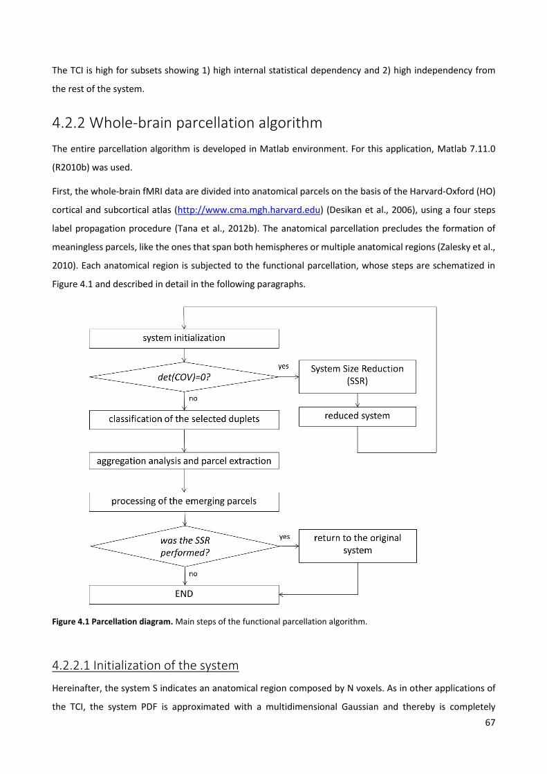
The present chapter deals with the issue of removal of the cardiac-related artefact that contaminates the

EEG signals recorded in an MR scanner at 3T, which still represents the main challenge of EEG and fMRI

integration. Different correction methods based on OBS followed by ICA are compared, with the objective to

set the proper parameters for ICA correction. The quality of correction is evaluated on resting-state data,

where the discrimination of the artefact from the information of interest is particularly difficult, but at the

same time an accurate correction is extremely important.

The chapter content is object of the paper entitled “Removal of pulse artefact from EEG data recorded in MR

environment at 3T. Setting of ICA parameters for marking artefactual components: application to resting

state data” by Eleonora Maggioni, Jorge Arrubla, Tracy Warbrick, Jürgen Dammers, Anna M. Bianchi, Gianluigi

Reni, Michela Tosetti, Irene Neuner and N. Jon Shah, published in PLOS ONE journal (2014, DOI

10.1371/journal.pone.0112147).

2.1 Introduction

As extensively described in the Introduction of the thesis, the combination of EEG and fMRI techniques can

provide a non-invasive comprehensive view of brain activity with high temporal (EEG) and spatial (fMRI)

resolution.

An interesting application of simultaneous EEG-fMRI is the study of brain during resting-state. The

spontaneous electrophysiological activity exerts a large influence on sensory, cognitive and motor-driven

processes (Varela et al., 2001; Engel et al., 2001) and contributes to the total variance of brain electrical

activity much more than the evoked/event-related responses (Raichle, 2006). Several fMRI studies showed

the presence of multiple specific functional large-scale networks during rest, called Resting-state Networks

(RSNs). During rest, functional connectivity patterns have been detected in the default mode network (DMN),

i.e. a cohesive network supporting a default mode of brain function that appears deactivated during cognitive

tasks (Greicius et al., 2003), and in networks representing specific systems, of which some examples are the

motor system (Biswal et al., 1995), the language system (Hampson et al., 2002), the attention system (Fox et

al., 2006) and the working memory system (Mazoyer et al., 2001).

19

Despite growing knowledge of BOLD RSNs, their underlying electrophysiological signature is still a matter of

discussion. One of the main topics to clarify is how the coherent slow fMRI hemodynamic fluctuations are

coupled to the fast neuronal activity recorded with EEG: this question can be addressed by inspecting BOLD

correlates to EEG microstates (Britz et al., 2010), with joint Independent Component Analysis (Moosman et

al., 2008) or studying multimodal functional network connectivity (Babiloni et al., 2008).

However, a meaningful exploitation of EEG-fMRI information relies on good data quality, especially in the

case of resting-state applications. Indeed, while in the study of event-related brain response the interesting

information is usually restricted to a group of channels and is known a priori, in resting-state analysis the

global state of the brain is of interest.

The main concern of EEG-fMRI integration regards the removal of artefacts from the EEG signal recorded in

the MR environment. The largest artefact affecting the EEG signal is the gradient artefact, caused by the

switching of magnetic field gradients required for MR image acquisition. Despite its huge amplitude, since it

occurs at fixed time intervals, it is easily removable by subtracting an average GA template from the EEG

signal at the channel level (Allen et al., 2000).

A second type of artefact is the pulse artefact, indirectly generated by cardiac activity. Although the PA

amplitude is smaller than that of GA, its removal is more challenging. The PA is highly non-stationary over

space and time and exhibits high inter and intra-subject variability.

Three factors mainly contribute to PA: first, a ballistic effect is considered to be caused by pulsatile body

motion, probably due to the acceleration and abrupt reversal in blood flow in the aortic arch (Mullinger et

al., 2013). The movement of electrically conductive material in a static magnetic field leads to

electromagnetic induction; therefore, the body’s pulsatile movement causes electromotive forces (EMFs) in

the EEG recording system, which in turn affect the registered EEG signal. Additional EMFs are caused by a

slight rotation of the head, probably produced by changes of pulsatile blood flow momentum in the cranial

arteries (Neuner et al., 2013a)). The third main contribution to PA is given by the Hall effect, related to the

movement of a conductive fluid (blood) in a static magnetic field, which induces electrical potentials recorded

at the scalp level (Neuner et al., 2013b)).

The combination of these factors increases the spatial and temporal complexity of the PA. Up to now, several

methods have been proposed for its removal. A first category of techniques operates at the channel level by

subtracting a template of the artefact, which is commonly estimated by 1) performing a dynamic average of

the artefact across its occurrences, as done in the AAS method (Allen et al., 2000) or 2) using the first (usually

3) principal components of the signal corresponding to PA intervals, as performed in the OBS method (Niazy

et al., 2005). Both the techniques remove the majority of the artefact, but none of them is able to correct

the EEG signal completely.

20

As an alternative to channel-based techniques, Blind Source Separation (BSS) techniques have been

proposed, among which ICA (Comon, 1992) is most commonly used. ICA is used to remove EEG artefacts due

to eye blinking or movements (Jung et al., 2000) and the ones related to the MR environment (Srivastava et

al., 2005; Briselli et al., 2006; Mantini et al., 2007). ICA decomposes the signal into sources that are maximally

independent over time; following the assumption that sources of PA are independent from neuronal ones,

ICA appears to be a suitable technique for retrieving the underlying neuronal information.

However, for the ICA decomposition to be meaningful, the sources should be stationary in space, and often

this is not the case with EEG signals. Indeed, not only the spatial topography of PA contribution changes

during the cardiac cycle, but also the neuronal signals themselves can be strongly non-stationary over time.

More than one work confirmed the ability of ICA to remove the PA (Srivastava et al., 2005; Mantini et al.,

2007), but in the literature there are also reported cases of poor ICA performance (Grouiller et al., 2007;

Debener et al., 2005; Debener et al., 2007). The unmet requirement of stationarity could be one of the

reasons for the possible failure of ICA algorithm. Besides that, the tuning of ICA parameters and the

identification of the PA-related Independent Components (ICs) are challenging.

Recently it was proposed to apply OBS before ICA in order to 1) help in meeting the ICA assumptions and 2)

check if the ICA performance could improve if a reduced amount of artefact was present. The OBS-ICA

combines the strengths of both approaches and was confirmed capable of improving satisfactorily the

corrections (Debener et al., 2007; Vanderperren et al., 2010) compared with the single techniques.

Nevertheless, the ICA correction entails the risk of deteriorating the EEG signal; the ICA step is performed on

a signal already subjected to OBS and less contaminated by artefacts than previously, making the PA

contribution in the resulting components less noticeable. This makes the selection of artefactual components

a very delicate task. The discrimination between physiological and artefactual components can be performed

either by manually inspecting the components (e.g. (Britz et al., 2010)) or by using semi-automatic or

automatic methods. Although several research groups performed the correction by manually selecting the

PA-related components (Nakamura et al., 2006; Huiskamp, 2006), the manual approach relies significantly

on the user’s experience and cannot be recommended as a routine procedure. Among the automatic

selection criteria, the most common ones look either at the amount of correlation that the ICs share with the

electrocardiographic (ECG) signal or a PA template (Srivastava et al., 2006) or at the amount of PA variance

explained by the ICs (Debener et al., 2008).

Vanderperren and colleagues (2010) inspected the effects of several PA correction methods on the quality

of visual event-related potentials. They performed an extensive comparison between OBS, ICA and OBS-ICA,

using for each of these techniques different parameters settings; the most used algorithms for ICA calculation

were compared, together with criteria for selection of artefactual ICs. Although the ERPs have been largely

object of investigation, up to now the impact of different PA corrections on resting-state data has not been

21

sufficiently debated. In these data the information of interest is largely unknown, therefore an optimal

canceling of EEG artefacts is extremely important.

Starting from the assumption that OBS-ICA has the potential to improve the quality of EEG signal retrieval

(Debener et al., 2007; Vanderperren et al., 2010), we focus on this combined approach with the objective to

define 1) an appropriate time interval for computation of the ICA mixing matrix and 2) an adequate criterion

for selection of artefactual components, as applied to resting-state EEG data recorded at 3T.

In the present chapter, two time intervals for ICA calculation are compared, together with four criteria for

marking the artefactual components. The different methods are evaluated in terms of their capability to 1)

reduce the amount of PA and 2) preserve the information of interest, which for the sake of simplicity is

identified as the alpha rhythm in the occipital channels. The comparison is performed on a group of 12

healthy volunteers who underwent EEG-fMRI acquisition during two separate periods of rest interleaved by

a cognitive task. The performance of each ICA correction is tested on the two resting-state datasets

separately. The results of the ICA corrections on the two groups of datasets are compared, with the aim of

assessing their reliability and reproducibility.

2.2 Materials and methods

2.2.1 Subjects

Twelve healthy right-handed volunteers with no history of neurological disorders took part to the study (9

males, mean age = 27.7 ± 6.6 years). All of them signed a written informed consent to the protocol, in

accordance with local ethical committee guidelines.

2.2.2 EEG-fMRI data acquisition

All EEG data were recorded simultaneously with fMRI recordings in a Siemens 3T Trio MR scanner (Germany).

EEG data were acquired using an MR-compatible EEG system (Brain Products, Gilching, Germany). The EEG

cap (BrainCap MR, EasyCap GmbH, Breitbrunn, Germany) included 63 scalp electrodes distributed according

to the 10-20 system and one additional ECG electrode placed on the participants’ back. EEG signals were

acquired relative to an FCz reference, with the ground in correspondence of Iz (10-5 electrode system). The

EEG data were sampled at 5000 Hz, with a band-pass filtering of 0.016-250 Hz. The impedance at each

electrode was kept lower than 10 kΩ.

2.2.3 Protocol

The study protocol was approved by the local human subjects review board at RWTH Aachen University and

was carried out in accordance with the Declaration of Helsinki. Two phases of rest lasting 6 minutes (i.e. 180

22

fMRI scans) were separated by 3 runs of a visual oddball task lasting 10 minutes and 8 seconds (i.e. 304 fMRI

scans) per run. During resting wakefulness, the subjects were asked to keep their eyes closed. The analysis

was performed only on the EEG resting-state recordings, as the data from the visual oddball task are

presented elsewhere (Warbrick et al., 2013 a), b)).

2.2.4 EEG data processing

A schematic illustration of the entire processing stream is shown in Figure 2.1. The EEG data were first

cleaned by GA and downsampled to 250 Hz with BrainVision Analyzer 2.0 software (BrainProducts, Gilching,

Germany). The imaging artefact was corrected by subtracting from each channel a template, which was

created using a sliding average of 21 GA blocks.

In preparation for PA correction, the R peaks were identified using the specific tool provided by Analizer 2.0

in semi-automatic modality. The first R peak was semi-automatically selected from a well-defined QRS

complex and used as a template for the identification of all the others. The correct position of the R peaks

identified by the software was verified by the user and corrected where necessary. Then, the EEG raw data

were exported into Matlab 7.11.0 (R2010b) and the FMRIB plug-in of the EEGLAB toolbox (version 11.0.5.4b)

(Delorme and Makeig, 2004) was used to perform the OBS correction, where the default parameters were

used, that is, a basis set of the first 3 principal components was the PA template.

To reject the residual PA, the EEG signals were reimported into Analyzer 2.0 and segmented from the fifth

fMRI scan onwards. Then, the extended infomax ICA (Lee et al., 1999) was applied. The ICA mixing matrix

was computed considering either the whole data (ICA_whole) or epochs lasting from 0 to 700 ms with respect

to (w.r.t.) the R peaks, which will be referred to as PA intervals (ICA_R). The components resulting from each

ICA calculation were segmented into PA intervals and further analyzed. The PA-related components were

identified following four different methods; the first three were implemented in Matlab scripts, whereas the

fourth was a function of Analyzer 2.0. The comparison regarded eight ICA-based methods, resulting from the

combination of the two types of ICA calculation (ICA_whole and ICA_R) and the four criteria for selecting the

PA-related ICs. These parameter settings were evaluated separately on the two groups of datasets, relative

to the resting-state periods preceding (Dataset1) and following (Dataset 2) the cognitive paradigm.

23

Figure 2.1 EEG processing diagram. Schematic illustration of the EEG data processing.

2.2.4.1 Selection of PA related components

The thresholds of the automatic selection criteria were chosen on an empirical basis, expressly equal across

subjects.

Variance contribution (pvaf)

Each component was back-projected to the EEG signal space, and the variance of the resulting signal across

the PA intervals was calculated and compared to the initial EEG variance during the same intervals, following

the same procedure described in (Vanderperren et al., 2010; Debener et al., 2008). The comparison relative

to one representative IC is displayed in Figure 2.2 a). The ICs that explained more than the 2.5% of the initial

variance were marked as PA-related and removed.

Correlation (corr)

We evaluated the cross-correlation between each IC and two PA templates. Since the cardiac-related artefact

changes polarity from one side of the head to the other (Debener et al., 2008; Vanderperren et al., 2007),

one template for each hemisphere was used. Each template was created by averaging the EEG uncorrected

signals (before OBS) over the PA intervals and over the left/right EEG channels (the mesial channels were

included in both templates). In Figure 2.2 b), the templates relative to one exemplar subject are plotted.

Instead of using an absolute correlation threshold, we used as reference the maximum correlation between

each template and the ICs, marking as cardiac-related the ICs whose correlation with one of the templates

24

was higher than the 40% w.r.t. the maximum. The choice of a relative threshold in place of an absolute one

was motivated by the differences in correlation coefficients across subjects.

Partial autocorrelation function (pacf)

Blocks formed by four consecutive PA intervals were averaged and the partial autocorrelation function was

calculated, similarly to that performed in (Vanderperren et al., 2010). The ICs with a peak at R-R distance lag

were selected (an exemplar PACF with R-R peak is in Figure 2.2 c)). Among them, the ICs with a peak

amplitude higher than one third of the maximum across ICs were removed.

Wavelets analysis (wave)

For each IC, the mean continuous wavelets transform (CWT) across PA intervals was calculated. We used the

Morlet complex family of wavelets (central frequency=14.591Hz, bandwidth=5.836 Hz) and investigated

frequencies going from 1 Hz to 20 Hz with twenty steps in between. Taking as reference the time-varying

frequency content of the PA templates, the ICs having a peak time locked to the R peak between the delta

and alpha band were identified as artefactual and removed. Figure 2.2 d) shows the CWT of an exemplar PA

template.

This selection method, which has not been used in previous studies, was created in the attempt to emphasize

the frequency contributions time-locked with the cardiac cycle, which characterize the PA-related

components. The selection was performed by one person, who was trained on the inspection of ICs and their

time-frequency transforms for a period of two and a half months.

25

Figure 2.2 Overview of methods for selection of PA-related components. a) pvaf method: variance contribution of one exemplar component (IC backprojection in red, original EEG in black), b) corr method: PA templates of one subject (left hemisphere in blue, right one in green), c) pacf method: PACF of one representative IC, with peak at the R-R distance, d) wave method: wavelets transform (instantaneous amplitude, Gabor normalization) of one representative PA template.

2.2.4.2 Validation criteria

To check the quality of PA removal, EEG epochs from -200 ms to 1 s w.r.t. R peaks, before and after ICA

correction, were extracted and compared. We will referred to them as R epochs. The performance of the

different ICA corrections was assessed by means of three different criteria. When the effects of PA correction

on the alpha content were examined, only the occipital channels were considered, otherwise all the EEG

channels were used. In each validation, the quality measures of the eight ICA-based methods were compared

through a non-parametric Kruskal Wallis (KW) test, for each dataset separately; if significant differences

emerged at the group level, the KW statistics were used in a multiple comparison test to extract the pairwise

differences. This was followed by two further comparisons, between 1) the four selection methods (across

datasets and ICA intervals) and 2) the two ICA intervals (across datasets and selection methods).

26

Peak to peak (PTP) ratio

Assuming the maximum signal variation (peak to peak distance) to correspond to PA, the ratio between the

peak to peak value after and before ICA correction provides a measure of the amount of artefact removed

by ICA. This ratio, averaged over all the EEG channels, was therefore used to estimate the effectiveness of

the PA correction.

Batch frequency content (BFC)

For each subject and channel, before and after ICA correction, the power spectral densities (PSD) of

consecutive R epochs were estimated using an autoregressive (AR) method.

The PA shows a main contribution in the low frequency range (between around 4 and 8 Hz) and an additional

one in the alpha range (from 8 to 13 Hz). Therefore, the reduction in spectral power in these bands induced

by ICA correction can give information on the amount of artefact removed.

However, the preservation of the resting-state rhythms should also be checked. For this purpose, subjects

having an evident alpha peak in the mean PSD before ICA correction were selected (Subj4, Subj9, Subj11 and

Subj12) with the aim of checking if the alpha rhythm could be retrieved after ICA correction. In these subjects,

the neuronal alpha rhythm contributes to the alpha power more than the artefact, therefore a good PA

correction should remove as much of the low frequency contribution as possible while maintaining most of

the alpha power. In each subject, we averaged the PSDs across R epochs and occipital channels (O1, O2 and

Oz) and looked at the ratio between delta (delta_ratio), theta (theta_ratio) and alpha (alpha_ratio) power

after and before ICA. Additionally, we defined a Quality Coefficient (QC) as the ratio between the alpha ratio

and the delta and theta ratios: such a measure is proportional to the amount of 1) low frequency power

cancelled and 2) alpha power preserved.

In addition, a comparison including all subjects and channels was performed (group_test). In each subject,

we averaged the PSDs across R epochs and EEG channels and looked at the ratio between delta (delta_ratio)

and theta (theta_ratio) power after and before ICA. In this case, the previous assumptions on the alpha

contribution were no longer reliable, therefore the quality of correction was evaluated just in terms of the

proportion of delta and theta power that was removed.

Time-varying frequency content (TFC)

The batch frequency content might not provide sufficient information to evaluate the correction quality. In

resting-state data, for example, the percentages with which PA and neuronal signals contribute to the total

alpha power are not known a priori, therefore it is difficult to state whether the physiological alpha rhythm

is preserved or not just by looking at the change in alpha power.

The time-varying frequency content can provide further details on the effects of ICA correction on the original

signal. Indeed, a good correction can be assessed by looking at the continuous frequency components

27

(physiological) compared to the PA-locked ones (artefactual), without having any a priori knowledge of their

contribution to the total power. By averaging across R epochs, the contributions synchronous with cardiac

cycle are emphasized. An example of physiological vs. artefactual frequency contributions is provided in

Figure 2.3, where the CWTs associated with two independent components of the EEG signal are compared.

For each subject and EEG channel, we computed the mean CWT across R epochs using a Morlet wavelet

(central frequency=0.8125 Hz), before and after ICA correction. Absolute CWT values were considered. We

averaged the CWTs across all subjects and 1) all channels or 2) only the occipital ones: in the latter, we

expected to find a continuous alpha contribution, in particular after ICA correction.

We emphasized the time-frequency components that were removed from each ICA correction by subtracting

the group CWT of the corrected signal (CWTpost) from the group CWT of the uncorrected signal (CWTpre). After

visual inspection of such difference, called CWToff, we used its time derivative (averaged over both time and

frequency) as metric for the correction quality. Since physiological and PA-related frequency components are

associated with low and high values of derivative, the selection methods corresponding to higher mean

derivatives (MD) of CWToff were evaluated better than others.

Figure 2.3 Artefactual versus physiological components: example. Mean CWT (absolute values) across PA intervals of two independent components of the EEG signal of one representative subject (before ICA correction). One component is artefactual (panel a) and one is physiological (panel b).

28

2.3 Results

Across datasets and ICA intervals, it emerged that the pvaf method led to the removal of less components

compared to the others, with 9.2 out of 63 ICs removed on average, against 19.6 of the corr method, 21.4 of

the wave method and 20 of the pacf method. The results of each validation method relative to both the

datasets are shown below.

2.3.1 PTP ratio

The comparison in terms of PTP ratio (of which Figure 2.4 provides an example) revealed differences in the

eight ICA correction methods in terms of their effectiveness in reducing the PA amplitude. The values of PTP

ratio (25, 50 and 75 percentiles across subjects) associated with the eight ICA-based methods are listed in

Table 2.1.

The findings of the two datasets were in agreement. The ICA calculation on the whole signal combined with

the pvaf method for the selection of PA-related ICs (pvaf_whole) led to the best results in terms of PTP ratio.

The KW test between the eight methods showed significant differences only in Dataset2 (p<0.05): the

following multiple pairwise comparison showed that when the ICA matrix was calculated from the whole

dataset, the pvaf method (pvaf_whole) performed significantly better than the corr method (corr_whole)

(p<0.05). By comparing the four selection methods across ICA intervals and datasets, significant differences

emerged (p<0.01). In particular, the pvaf method performed better than the corr method (p<0.01) and pacf

method (p<0.05), whereas no significant differences were detected with respect to the wave method. The

statistical test between the two ICA intervals showed no significant differences; indeed, the performance of

ICA_whole with respect to ICA_R was variable and dependent on the selection method and the dataset under

examination.

29

Figure 2.4 PTP ratio: example. PTP ratio comparison relative to the Oz channel of one subject. The maximum variation of EEG signal before (black curve) and after correction with ICA were compared, using the two ICA calculations (ICA_whole on the left, ICA_R on the right) and the four methods for selection of components. The color legend is at the top left of each plot.

Table 2.1 PTP ratio (25, 50 and 75 percentiles across subjects) of each ICA correction (ICA_whole and ICA_R) in the two Datasets.

2.3.2 BFC

The comparison between the eight ICA-based methods based on their frequency content led to partially

conflicting results. Indeed, while the group_test results were in line with the PTP value results, the QC_test

provided discordant information with respect to them.

The group_test (including all the subjects and all the EEG channels) confirmed the capability of the pvaf

method to remove the low frequency artefactual contribution. The values of the ratio between the delta and

theta power after and before the eight ICA corrections are listed in the upper panels of Table 2.2 (Dataset1)

and Table 2.3 (Dataset2). Significant differences were found between the methods (p<0.01 in both datasets).

ICA_whole pvaf corr wave pacf

25 50 75 25 50 75 25 50 75 25 50 75

Dataset 1 0,66 0,71 0,79 0,69 0,78 0,93 0,73 0,79 0,88 0,66 0,79 0,92

Dataset 2 0,63 0,71 0,76 0,79 0,87 0,91 0,72 0,76 0,87 0,73 0,79 0,90

ICA_R pvaf corr wave pacf

25 50 75 25 50 75 25 50 75 25 50 75

Dataset 1 0,68 0,73 0,81 0,73 0,83 0,86 0,60 0,70 0,85 0,63 0,72 0,89

Dataset 2 0,68 0,73 0,77 0,77 0,85 0,94 0,69 0,77 0,89 0,74 0,87 0,95

30

In Dataset1, the pvaf_whole method removed significantly more low frequency (LF) power than corr_whole

(p<0.01), wave_whole (p<0.03), pacf_whole (p<0.01) and corr_R (p<0.04) methods. In Dataset2, the

pvaf_whole method removed significantly more LF power than corr_whole (p<0.01), wave_whole (p<0.01),

corr_R (p<0.03) and pacf_R (p<0.04) methods. Summarizing across datasets and intervals used for ICA

calculation, the selection based on variance led to the greatest removal, followed by the wave, pacf and corr

selection methods. The KW analysis showed a significant difference among these methods (p<0.01), with the

pvaf method significantly different from the other three (p<0.01). No significant differences were identified

between the two intervals for ICA calculation (ICA_whole and ICA_R).

The results of the QC_test (only on the occipital channels of the four subjects with alpha peak) are listed in

Table 2.2 and Table 2.3 for Dataset1 and Dataset2 respectively. These tables include the ratio between the

delta, theta and alpha power after and before ICA correction. The KW analysis performed on the eight

methods with each of the computed measures (QC, delta_ratio, theta_ratio and alpha_ratio) showed no

significant differences.

Nevertheless, we could identify differences in the eight ICA-based methods’ performance. In contrast with

the PTP ratio validation, the pvaf method had the lowest QC, regardless of the interval used for ICA

calculation, as it reduced the low-frequency range power more than the others but also cancelled the

majority of the alpha power. By comparing the two ICA intervals (across datasets and selection methods) and

the four selection methods (across datasets and ICA intervals) separately, no significant differences emerged.

However, the wave selection method had the highest QC value (median= 0.90), immediately followed by corr

(median= 0.89) and then by pacf (median= 0.76) and pvaf (median= 0.71) ones respectively. Figure 2.5 shows

for one representative subject the occipital spectral content across PA epochs, before and after ICA

correction with the four selection methods.

Table 2.2 Spectral coefficients (25, 50 and 75 percentiles across subjects) of each ICA correction in Dataset1. Group_test: delta+theta ratio, averaged over all subjects and channels. QC_test: QC, alpha ratio, delta ratio and theta ratio averaged over the occipital channels of the four subjects with alpha rhythm.


25 50 75 25 50 75 25 50 75 25 50 75

Group test

Delta+theta ratio

0.80 0.86 0.9 0.97 1.38 1.76 1.07 1.39 1.52 1.01 1.35 1.69

QC test

QC 0.48 0.89 1.17 0.86 0.94 1.49 0.74 1.02 1.50 0.70 0.80 1.12

Delta_ratio 0.42 0.50 0.56 0.59 0.75 0.96 0.52 0.58 0.72 0.61 0.86 1.05

Theta_ratio 0.29 0.41 0.59 0.58 0.77 0.87 0.40 0.47 0.69 0.58 0.85 0.95

Alpha_ratio 0.22 0.42 0.61 0.65 0.79 0.94 0.48 0.72 0.78 0.55 0.71 0.80

31

Table 2.3 Spectral coefficients (25, 50 and 75 percentiles across subjects) of each ICA correction in Dataset2. Group test: delta+theta ratio, averaged over all subjects and channels. QC_test: QC, alpha ratio, delta ratio and theta ratio averaged over the occipital channels of the four subjects with alpha rhythm.


25 50 75 25 50 75 25 50 75 25 50 75

Group test

Delta+theta ratio

0.82 0.93 1.01 0.94 1.38 1.62 0.94 1.08 1.26 0.94 1.07 1.44

QC test

QC 0.48 0.71 0.91 0.56 0.86 1.38 0.69 0.93 1.44 0.56 0.77 1.16

Delta_ratio 0.51 0.57 0.63 0.53 0.58 0.69 0.48 0.53 0.79 0.58 0.58 0.79

Theta_ratio 0.35 0.42 0.56 0.35 0.39 0.61 0.40 0.46 0.60 0.45 0.54 0.74

Alpha_ratio 0.24 0.34 0.49 0.26 0.56 0.78 0.40 0.60 0.75 0.30 0.58 0.80


25 50 75 25 50 75 25 50 75 25 50 75

Group test

Delta+theta ratio

0.75 0.88 1.04 1.47 1.64 1.71 1.32 1.48 1.63 1.1 1.48 1.60

QC test

QC 0.51 0.70 0.88 0.67 0.88 0.97 0.72 0.82 0.99 0.51 0.65 1.06

Delta_ratio 0.50 0.55 0.78 0.87 0.98 1.09 0.57 0.83 0.86 0.53 0.71 0.84

Theta_ratio 0.36 0.47 0.54 0.80 0.83 0.98 0.47 0.70 0.80 0.46 0.59 0.81

Alpha_ratio 0.28 0.32 0.45 0.65 0.76 0.84 0.42 0.66 0.78 0.34 0.41 0.63


25 50 75 25 50 75 25 50 75 25 50 75

Group test

Delta+theta ratio

0.86 0.92 1.06 1.03 1.40 1.71 1.21 1.45 1.51 1.17 1.41 1.65

QC test

QC 0.6 0.71 1.01 0.75 0.85 0.95 0.82 0.99 1.19 0.69 0.84 1.36

Delta_ratio 0.45 0.57 0.75 0.86 0.93 1.11 0.44 0.60 0.75 0.53 0.74 0.94

Theta_ratio 0.39 0.55 0.75 0.82 0.84 0.94 0.41 0.56 0.62 0.47 0.72 0.97

Alpha_ratio 0.33 0.48 0.59 0.70 0.75 0.86 0.41 0.47 0.68 0.49 0.80 0.93

32

Figure 2.5 BFC: example. AR power spectral density across EEG epochs relative to the occipital channels of one representative subject, before and after ICA correction with the four selection methods. The spectral contents were averaged across the PA intervals (ICA_whole and ICA_R).

2.3.3 TFC

The visual inspection of the CWToff of each ICA correction, representing the time-varying frequency

components removed at the group level, allowed us to easily discriminate between poor and good

corrections. The qualitative and quantitative comparisons based on CWToff_occ (occipital channels) and

CWToff_all (all channels) confirmed the higher reliability of the wave method with respect to the pvaf one in

preserving the information of interest.

The results of the quantitative comparison based on the CWToff mean derivative are described hereinafter.

The MD values are listed in Table 2.4 (Dataset1) and Table 2.5 (Dataset2). In the analysis of CWToff_all, the KW

statistics showed significant differences between the eight ICA corrections (p<0.01 for both datasets).

Looking at the pairwise comparisons, in Dataset1, the wave_R method performed significantly better than

corr_R method (p<0.03), whereas no significant pairwise differences emerged in Dataset2. No significant

differences emerged from the comparison between the two ICA intervals (across datasets and selection

33

methods), whereas the comparison between the four selection methods showed significant differences

(p<0.01), with the corr and pacf methods significantly worse than the wave and pvaf methods (p<0.01). In

particular, the wave method was first-ranked, followed by pvaf, pacf and corr methods.

Similar results emerged from the analysis of CWToff_occ, where significant differences were found between

the eight ICA corrections in Dataset1 (p<0.03), but not within the single pairs of methods. Again, significant

differences emerged between the four selection methods but not between the two ICA intervals (p<0.01).

The rank was the same as in CWToff_all. The pairwise comparison showed that the corr method was

significantly worse than pvaf and wave methods (p<0.01), while the pacf method was just worse than the

wave method (p<0.02).

These quantitative findings were confirmed by the visual inspection of CWToff and CWTpost (especially the

ones relative to occipital channels), from which emerged the capability of the wave method to remove the

PA-locked alpha while leaving intact the continuous alpha. The visual inspection proved the poor

performance of the corr method, which left the artefactual contribution untouched, and confirmed the

tendency of the pvaf method to remove information of interest. The pacf method performed better than

corr but worse than wave and pvaf methods.

The CWTpost_occ and the CWToff_occ of the eight ICA corrections, relative to Dataset1, are shown as example in

Figure 2.6 (ICA_whole) and Figure 2.7 (ICA_R). Whichever ICA interval was used, the CWTs after ICA

correction (on the left panels) show how the wavelet method left the most continuous alpha contribution,

although it removed the low frequency artefactual contribution less than the pvaf method. Further

confirmation can be found by looking at the CWToff_occ (right panels), displaying that 1) the wave method

removed only the PA-related alpha and 2) the pvaf method removed the PA more than the others but

together with a portion of continuous alpha power.

Table 2.4 Mean derivative of CWToff (time-frequency transform of the EEG signal removed by ICA correction) corresponding to each ICA correction in Dataset1. CWToff_all: averaged over all channels. CWToff_occ: averaged over occipital channels.


25 50 75 25 50 75 25 50 75 25 50 75

MD CWToff_all 0.61 0.73 0.89 0.40 0.43 0.51 0.59 0.81 1.02 0.27 0.39 0.51

MD CWToff_occ 0.58 0.69 1.04 0.31 0.40 0.49 0.59 0.81 1.15 0.37 0.44 0.58


25 50 75 25 50 75 25 50 75 25 50 75

MD CWToff_all 0.64 0.76 0.85 0.25 0.36 0.45 0.72 0.91 1.13 0.37 0.51 0.63

MD CWToff_occ 0.67 0.78 1.05 0.31 0.47 0.66 0.71 0.91 1.20 0.54 0.67 0.77

34

Table 2.5 Mean derivative of CWToff (time-frequency transform of the EEG signal removed by PA correction) corresponding to each ICA-based method in Dataset2. CWToff_all: averaged over all channels. CWToff_occ: averaged over occipital channels.

Figure 2.6 TFC results, ICA_whole. Group CWT (absolute values). Left: CWT of the EEG signals after correction (CWTpost) with the four selection criteria, averaged across R epochs and occipital channels. Right: CWT of the EEG signal removed by each ICA correction (CWToff), averaged across R epochs and occipital channels. The shown correction is relative to ICA calculation based on whole data (ICA_whole).


25 50 75 25 50 75 25 50 75 25 50 75

MD CWToff_all 0.60 0.75 0.90 0.19 0.27 0.30 0.59 0.80 1.05 0.22 0.30 0.31

MD CWToff_occ 0.46 0.63 1.01 0.18 0.31 0.39 0.59 0.89 1.24 0.30 0.42 0.56


25 50 75 25 50 75 25 50 75 25 50 75

MD CWToff_all 0.62 0.7 0.77 0.25 0.34 0.48 0.57 0.81 1.04 0.33 0.39 0.46

MD CWToff_occ 0.45 0.62 0.83 0.23 0.26 0.44 0.51 0.83 1.22 0.27 0.40 0.59

35

Figure 2.7 TFC results, ICA_R. Group CWT (absolute values). Left: CWT of the EEG signals after correction (CWTpost) with the four selection criteria, averaged across R epochs and occipital channels. Right: CWT of the EEG signals removed by each ICA correction (CWToff), averaged across R epochs and occipital channels. The shown correction is relative to ICA calculation based on the PA intervals (ICA_R).

2.4 Discussion

In this section of the thesis, our objective was to identify the optimal ICA parameters for removal of the

cardiac-related artefact from EEG data recorded in MR environment. In particular, we discussed the quality

of PA removal on resting-state EEG data recorded at 3T. In resting-state data, the global information is of

interest and a very accurate correction is an essential step for any further analysis.

We compared two intervals for the calculation of the ICA mixing matrix, 1) the entire signal and 2) the PA

intervals, together with four methods for selecting the PA-related ICs, based on their 1) contribution to the

artefact variance, 2) correlation with PA templates, 3) wavelets transform and 4) partial autocorrelation

function. The quality of the EEG cleaning was assessed by looking at the changes occurring after ICA

correction in the EEG signal around the R peaks (from -200 ms to 1 s after it). Three different criteria were

considered, based on the EEG 1) peak to peak amplitude, 2) batch spectral content and 3) time-varying

spectral content. The comparison was performed on two groups of datasets relative to the same 12 subjects:

36

the general agreement between the outcomes of the two comparisons highlighted the reliability of each ICA

correction, whose performances were usually reproducible across datasets. The selection of PA-related ICs

based on their wavelets transform emerged as the best compromise between the amount of removed PA

and the preservation of the neuronal alpha content.

2.4.1 Comparison with previous studies

To the best of our knowledge, this was the first time that different ICA-based PA corrections were compared

on EEG data recorded during resting wakefulness. Indeed, the widespread comparison between OBS, ICA and

OBS-ICA methods described in (Vanderperren et al., 2010) investigated the PA removal quality in ERP data

from visual tasks, following and extending a previous comparative analysis on auditory ERPs (Debener et al.,

2007). Grouiller et al. (2007) evaluated algorithms for removal of EEG artefacts looking at 1) the goodness of

retrieval of the alpha rhythm modulation from a block paradigm and 2) the correct identification of interictal

spikes; despite the similar application, they did not investigate the setting of ICA parameters.

In our study, we focused on OBS-ICA combination, found to be capable of improving the correction

performed by the single techniques (Debener et al., 2007; Vanderperren et al., 2010). Despite this

potentiality, the additional use of ICA after OBS involves the risk of affecting the quality of the underlying

neuronal signal. In resting-state data, such risk is especially high: since the information of interest is global

and not always predictable, the discrimination between neuronal and PA-related ICs is challenging.

Consequently, a proper method for selecting the artefactual components is needed.

In addition to the selection criteria already described in the literature, we added a method based on visual

inspection of the ICs wavelets transform averaged across the R epochs. The novel selection method emerged

as a valuable criterion for marking the PA-related components, particularly adequate when resting-state EEG

data have to be corrected.

2.4.2 Validation criteria and main findings

The quality of PA correction was evaluated from different perspectives. The PTP ratio comparison looked at

the reduction in the PA amplitude range due to ICA correction. However, this criterion provided information

regarding the amount of PA removal only, whereas the validations based on the frequency content change

were also potentially sensitive to the deterioration of the signal of interest; in this application, the latter was

identified as the alpha rhythm clearly visible in the occipital channels of four subjects (BFC validation, QC

test), and more in general as the frequency components unlocked to PA occurrence (TFC validation).

The BFC criterion inspected the modifications induced by ICA correction to the EEG batch frequency

spectrum, giving a quantitative measure of the power change in each band of interest (delta, theta, alpha).

This approach assumes that the PA spectrum is characterized by peaks at heart-rate frequency and its

37

harmonics (Vanderperren et al., 2007). We also assumed that the main PA contribution would occur in the

low frequency range and a smaller one in the alpha range, according to the frequency content of the PA

templates of all subjects.

A first quality check was performed on the occipital channels of the four subjects with a visible alpha peak,

where the PA contribution to the alpha band was estimated to be less than the neuronal one. The quality of

each ICA correction was assumed to be proportional to the percent of 1) removed low frequency power

(delta and theta bands) and 2) preserved alpha power. For this purpose, we defined a quality coefficient as

the ratio between the former and the latter. With respect to the PTP ratio comparison, this validation

accounted for both the artefact removal and the recovery of the underlying information; on the other hand,

the QC index completely discarded the presence of an artefactual contribution to the alpha power.

To make the statistical analysis stronger, we additionally evaluated the change in batch frequency power in

all subjects and channels. In this condition, we only investigated the amount of low frequency power that

was removed, because the assumptions on the predominance of alpha physiological content over the

artefactual one were not valid anymore.

The BFC validation provided more detailed information with respect to the PTP comparison, but was limited

by the impossibility to distinguish between PA-related and physiological contributions in a same frequency

band. The investigation of the time-frequency information proved to be more suitable for this purpose.

The TFC criterion inspected the modifications induced by ICA corrections to the EEG time-varying frequency

content. Since the PA-related frequency content was locked in time to PA occurrence, while the physiological

one was independent, we evaluated the quality of cleaning in terms of the capability to preserve the long

lasting contribution and cancel the one locked in time to the PA occurrence. In particular, we analyzed the

time-frequency components that were removed by each ICA correction (CWToff), both visually and

quantitatively. This criterion was the unique to distinguish the neuronal and PA-related frequency

contributions and provided valuable information for the quality assessment.

The results of the comparative analysis strengthen the need to consider different factors when assessing the

quality of PA correction. Indeed, the validation based on PTP ratio was able to measure the amount of

artefact removed, but not to detect the possible negative effects on the signal of interest. The latter

information was recovered just by looking at the frequency content. The two frequency-validation criteria

(BFC and TFC), introduced in our study, proved to be extremely useful in the assessment of the effects of

each ICA correction on the signal of interest. In our application, the QC and TFC validations showed that the

pvaf method (marked as the best method by the PTP ratio criterion) removed part of the neuronal alpha

signal, thus revealing its inability to discriminate between neuronal and PA-related components. On the

contrary, the higher reliability of the wavelets selection method emerged.

38

Summarizing the results of the three validation criteria across the two datasets, the selection of the PA-

related ICs based on their wavelets transform emerged as the best compromise between the reduction in

the PA amplitude and the preservation of the resting-state underlying information. Indeed, in most cases

looking at the mean CWT across PA intervals allowed us to distinguish easily between neuronal and

artefactual components, given the differences in their temporal properties. The wave method represents a

novelty of our comparison with respect to previous ones. Regarding the two signal lengths for ICA calculation,

i.e. the whole dataset or only the PA intervals, both of them led to acceptable results and none outperformed

the other, as determined by the quantitative comparisons. The variability in the performance of the selection

methods across the subjects of the group was hypothesized to be related to the overall quality of the EEG

acquisition, which in turn influences the goodness of the detection of the R peaks and the performance of

OBS and ICA decomposition.

2.4.3 Methodological limitations

In each selection method, the parameter setting is a crucial step that influences the number of selected

components and in turn the quality of correction. In our study, the corr, wave and pacf selection methods

removed more components than the pvaf method. Nevertheless, the latter affected the original signal more

than the others, as it removed the components with highest energy. This suggests that the information about

which components are removed is more relevant than the number of removed components.

In the selection based on variance, the performance relies on two parameters. The first is the interval on

which the explained variance is computed. In our study, we decided to choose one interval for all subjects,

but the fact that the highest variance contributions were found in the first components suggests that our PA

interval (from 0 to 700 ms after the R peaks) did not always match the PA occurrence. The threshold is the

second parameter that has to be set: in our study, the 2.5% threshold was chosen from empirical

observations. Higher thresholds, such as 5%, led to the removal of a few components (the first sorted by

energy), which typically did not fully resemble the artefact. Instead, the 2.5% threshold setting also allowed

to remove components with lower energy but artefactual. Obviously, the optimal threshold depends on the

considered interval.

In the selection based on correlation, two factors are determinant, i.e. the quality of the ECG signal or

template and the correlation threshold. In our study, we decided to use an artefact template instead of the

ECG signal, since the latter seemed to be different from the artefact occurrences in the EEG signal;

nevertheless, the poor results suggest that our template did not resemble the cardiac artefact, at least in the

majority of subjects. The reason for this could be that the template was estimated from the EEG signal before

OBS correction. Regarding the thresholds, the choice between absolute or relative threshold and the set of

the threshold value are not trivial.

39

The selection method based on wavelets has the major drawback of being manual, relying on the user’s

ability to recognize the PA frequency contributions. To optimize the quality of PA removal, the user has to

train himself to inspect the IC signals together with their time-varying spectral content. In the current

application, the performances of the wave method were not optimal, because the low frequency

contribution of the PA was not removed as efficiently as when using the pvaf method. After proper training,

the user may be able to identify all the artefactual components. However, the combination of visual

inspection and quantitative indices for the selection of components would be beneficial.

In our study, the most delicate step in the pacf selection method based was related to the setting of the

threshold. Since many ICs had a peak in correspondence of the R-R distance, we decided to remove only the

ones with a peak amplitude above a certain threshold, i.e. one third of the maximum amplitude. A

comparison between different thresholds would also be useful in this case.

It is worth mentioning that the overall performance of the selection methods strongly depends on the quality

of the ICA decomposition. In the presented application, we used the Infomax ICA algorithm, which was

proved to be effective when used for PA correction in (Vanderperren et al., 2010), with the extended option,

allowing for components with negative kurtosis. Nevertheless, in the majority of datasets the ICs signals

changed characteristics over time, sometimes mixing timeframes of cardiac-related activity with others of

neuronal activity. Debener et al., (2008) suggested that the distortion of ICA solutions might increase with

the MR scanner static magnetic field. Although the reason of the possible failure of ICA estimation is still

unknown, it could be partially ascribed to the unmet assumption of spatial stationarity of the sources. Besides

the importance of a proper selection criterion, the quality of ICA decomposition is of primary importance for

obtaining satisfactory results.

2.5 Conclusion

In this chapter, we focused on the phase of pre-processing of resting-state EEG data recorded in an MR

environment at 3T, in preparation for EEG-fMRI integration. A full exploitation of the potentials of resting-

state EEG-fMRI integration is possible only if an optimal cleaning of the EEG signal is performed. In this

respect, the most challenging step regards the correction of the cardiac-related artefact.

In this application, we corrected the PA by combining two techniques, OBS and ICA, and proved that this

combined approach can effectively improve the correction, but entails the risk of deteriorating the signal of

interest. The comparison between different ICA corrections provided valuable information on the methods

for selection of the artefactual components and on the assessment of the effects that each ICA correction

has on the EEG signal.

The selection method here proposed based on the ICs wavelets transform resulted able to highlight the PA-

related ICs, making them easily distinguishable from the neuronal ones. The results at 3T are overall

40

satisfactory, but further investigation would be required when moving toward higher magnetic field

strengths. The significant challenges related to PA correction in EEG data recorded at ultra-high field will be

the topic of the next chapter.

41

3

Characterization and cleaning of pulse artefact from EEG data recorded at 9.4T static magnetic field. Can the resting-state EEG information be recovered?

The present chapter is an extension of Chapter 2, “Removal of pulse artefact from EEG data recorded in MR

environment at 3T. Setting of parameters for ICA correction: application to resting-state data”, and shifts the

problem of rejection of the cardiac-related artefact to EEG data recorded at ultra-high field.

In the light of the great potential of EEG-fMRI integration at ultra-high magnetic field strength, we intend to

investigate the feasibility of recording resting-state EEG signals at 9.4T static field. At this field strength, the

cardiac-related artefact covers completely the EEG neuronal information and its removal is more and more

challenging than at 3T. Therefore, the algorithms that perform efficiently at 3T need to be further improved

for working at high field.

By taking as reference the EEG data recorded at 0T, the impact of ultra-high field on resting-state EEG

information is investigated, and different correction techniques based on ICA are compared on the basis of

their capability to recover the underlying physiological information.

3.1 Introduction

In recent years, the potentials of MRI have been enhanced by the advent of ultra-high field MR scanners (≥

7T), which allow to obtain high quality images with increased SNR, tissue contrast and spatial resolution. By

exploiting the susceptibility induced contrast, BOLD functional imaging is among the techniques that benefit

most of the ultra-high field strength. Indeed, high field fMRI can reach a spatial resolution that matches the

cortical columns and layers (Yacoub et al., 2008; Duyn et al., 2012).

Literature evidences report the increasing popularity of simultaneous EEG-fMRI, but few is known about the

feasibility of EEG-fMRI integration at ultra-high field, in which the attractiveness of this combined technique

further increases. At a glance, the coupling between the EEG widespread neuronal activity and the high-

resolution fMRI hemodynamic may seem poor, therefore it needs to be investigated. What is certain,

however, is that the enhanced spatial resolution of ultra-high field fMRI combined with the high temporal

resolution of EEG can provide information with a level of detail never reached before.

Despite this great possibility, the challenges of recording EEG signals within ultra-high field MR scanners are

significant. The main obstacle is represented by the cardiac-related artefact, whose properties have been

extensively described in the introductory paragraph of Chapter 2. The pulse artefact has an amplitude

42

proportional to the static field strength (Debener et al., 2008, Neuner et al., 2013a) and becomes prominent

at ultra-high field, to the point of hiding completely the underlying neuronal information.

The nature of this artefact has been investigated for increasing static field strengths up to 7T in (Debener et

al., 2008) and up to 9.4T in (Neuner et al, 2013a). Up until now, most EEG recordings at ultra-high field

strength have been performed in absence of simultaneous fMRI acquisitions: this allowed to avoid the

contribution of fMRI gradients to EEG signals, thereby focusing on the cardiac-related artefact itself. Not only

the amplitude of PA, but also its spatial variability and distortion were found to increase with the magnetic

field strength, thus making the cleaning of the EEG signal a great hurdle. However, Neuner and colleagues

demonstrated 1) the feasibility of EEG recordings within 9.4T static field (Neuner et al., 2013a), 2) the

possibility of recovering visual and auditory evoked potentials (VEP and AEP) (Arrubla et al., 2013; Neuner et

al., 2013a) and event-related spectral desynchronizations (Neuner et al., 2013a) recorded at 9.4T and 3) the

absence of significant alterations in the processing of sensorial stimuli caused by the ultra-high static field

(Arrubla et al., 2013). The authors were able to extract the VEP/AEP information by means of ICA, which was

used both to correct the PA and to select the information of interest. The latter was not always retrievable

from the EEG signal at the channel level, probably due to the presence of residual artefacts in the data

(Neuner et al., 2013a).

However, the study of task-related brain activity represents just one of the possible EEG-fMRI applications.

As highlighted in Chapter 2, a research field that is gaining increasing interest regards the investigation of the

brain activity during resting wakefulness. The fMRI resting-state experiments can exploit the EEG information

to 1) monitor the state of vigilance of the subject and 2) extract the main neuronal rhythms.

Recently proposed techniques for acquiring whole-brain high-resolution fMRI at 7T (De Martino et al., 2011,

Boyacioğlu et al., 2014) allow to study the global resting-state information at ultra-high field. The

simultaneous EEG-fMRI at ultra-high field strength could provide evidence on the connection between

columnar and laminar level hemodynamic phenomena and fast neuronal oscillations.

Nonetheless, the possibility of retrieving the resting-state information from EEG data recorded at ultra-high

field has not been assessed yet. As stated in Chapter 2, the cleaning of the EEG signals for resting-state

analysis is particularly delicate, as the information of interest is widespread and known a priori only to a small

extent. The alpha synchronization upon closing of the eyes was identified at 9.4T in (Neuner et al., 2013a;

Dammers et al., 2014). This important discovery, based on a block-design with open and closed eyes

alternated, paves the way to a more extensive investigation of pure resting-state data recorded at ultra-high

field.

In the present chapter, we aim to investigate 1) the modifications induced by the ultra-high static magnetic

field (9.4T) on the resting-state EEG characteristics, 2) the possibility of recovering the physiological resting-

state information from EEG data recorded at 9.4T and 3) the differences in performance of five sophisticated

43

techniques of PA rejection based on the combination of AAS, OBS and ICA, differing in the method for

selection of the artefactual components. For this purpose, resting-state EEG data acquired from five subjects

at two different magnetic strengths, 0T and 9.4T, are analyzed: the 0T data are used as reference for assessing

the amount of data contamination due to the ultra-high field and consequently the quality of PA cleaning. As

in previous EEG experiments at 9.4T (Arrubla et al., 2013; Neuner et al., 2013a), EEG signals were acquired at

ultra-high static field without simultaneous fMRI recordings. If reached, an adequate removal of the cardiac-

related artefact represents a first important step towards simultaneous EEG-fMRI acquisitions at 9.4T.


3.2.1 Subjects

EEG data were recorded from five healthy right-handed volunteers (5 males, mean age = 27.4 ± 1.9 years)

with no history of neurological disorders. Written informed consent to the study was obtained from all

subjects.

3.2.2 EEG data acquisition

EEG data were recorded using an MR-compatible EEG system (Brain Products, Gilching, Germany). The EEG

cap (BrainCap MR, EasyCap GmbH, Breitbrunn, Germany) included 31 scalp electrodes distributed according

to the 10-20 system and one additional ECG electrode placed on the participants’ back. EEG signals were

acquired relative to an FPz reference, with the ground electrode in correspondence of AFz (10-5 electrode

system). The electrode impedance was kept below 10 kΩ. The EEG data were sampled at 5000 Hz, with a

band-pass filtering of 0.016-250 Hz, while the helium pump of the MR system was kept running.

3.2.3 Protocol

The study protocol was approved by the local human subjects review board at RWTH Aachen University, in

compliance with the Declaration of Helsinki. EEG data were recorded at 0T and inside a Siemens 9.4T human

whole-body MR scanner (Siemens Medical Systems, Erlangen, Germany). To guarantee consistency between

the two recordings, the subjects stayed in supine position also during the acquisition at 0T. In this condition,

they were inserted in a mock scanner that contributed to create the sensation of the MR environment while

keeping null the static magnetic field. Within the 9.4T scanner, they were positioned in correspondence of

the isocentre. The subjects remained in resting wakefulness with the eyes closed during the entire

acquisition.

44


The EEG signal pre-processing was performed for the most part using Brain Vision Analyzer 2.0 (Brain

Products, Gilching, Germany). The 0T and 9.4T EEG data were downsampled to 250 Hz and subjected to a

band pass filter ranging from 1 to 40 Hz. The bad intervals, affected by significant movement artefacts, were

manually marked by the user and excluded from the following analysis. An extended Infomax ICA (Lee et al.,

1999) was applied to remove the ocular and movement-related artefacts. The 9.4T data were then subjected

to PA correction.

After semi-automatic identification of the R peaks (using the same procedure described in Chapter 2), a first

PA correction based on AAS method was performed, using a specific function of Analyzer 2.0. The AAS

correction allowed to remove a big portion of the PA. The so-cleaned EEG data were then exported into

Matlab 7.11.0 (R2010b) and further subjected to OBS correction with the default parameters using the FMRIB

plug-in of the EEGLAB toolbox (version 11.0.5.4b) (Delorme and Makeig, 2004). We deemed opportune to

combine AAS and OBS, which usually are performed alternatively, because the artefact caused by the 9.4T

static field was huge and extremely difficult to remove.

Since the two consecutive corrections were still not sufficient to remove the artefact completely, the EEG

data were reimported into Analyzer 2.0 and subjected to ICA-based correction of the residual PA. An

extended Infomax ICA was applied (Lee et al., 1999), in which the ICA mixing matrix was computed by

considering the whole EEG data: this choice was motivated by the results of the comparison between ICA-

based corrections at 3T, presented in Chapter 2, which showed no significant difference of performance

between the two intervals for calculation of the mixing matrix (whole data or PA intervals). Similarly to the

previous Chapter, the ICs were segmented into PA intervals, going from 0 to 700 ms w.r.t. the R peaks. These

segments were analyzed in order to identify the ICs related to PA. Five different criteria were used to identify

the artefactual components, i.e. the four used in the 3T comparison and an additional one. After application

of each selection method, the EEG data were reconstructed through inverse transform of the non artefactual

ICs. For each ICA correction (i.e. based on each selection method), we assessed the quality of removal of the

cardiac-related artefact from different perspectives, on the basis of 1) amount of artefact removed and 2)

comparison with the 0T information.

3.2.4.1 Selection criteria

The main steps characterizing the first four validation criteria are already described in Chapter 2. Some

differences regarded the considered intervals and the empirical thresholds used for selecting the artefactual

components.

45

Variance contribution (pvaf)

The same procedure described in Chapter 2 was followed, with the difference that the variance was

calculated on the intervals most affected by the artefact that were selected from subject to subject. The ICs

that explained more than the 5% of the initial variance were marked as PA-related and removed.

Correlation (corr)

The same procedure described in Chapter 2 was carried out. We marked as PA-related the ICs having a

correlation with one of the PA templates higher than the 50% w.r.t. the maximum correlation between each

template and the ICs. For each IC and template, the correlation coefficient was calculated by averaging the

ones calculated on the single PA intervals. As previously, the choice of a relative threshold in place of an

absolute one was justified by the different correlation coefficients that characterized the five subjects.

Wavelets analysis (wave)

The details on this selection criterion can be found in Chapter 2. The selection was performed by the same

trained person that performed it in the 3T comparison of Chapter 2.

Partial autocorrelation function (pacf)

As described in Chapter 2, the ICs with partial autocorrelation peak at R-R distance lag were selected: among

them, the ICs with a peak amplitude higher than 50% of the maximum peak across all components were

removed.

Cross Trial Phase Statistics (ctps)

A fully automated approach based on cross trial phase statistics (CTPS), which was introduced in (Dammers

et al., 2008), was used to identify the cardiac-related artefacts in the phase domain. The phase of each IC was

calculated by applying the Hilbert transform. The results were aligned across intervals going from -0.1 to 0.8

s w.r.t. the R peaks, and the phases corresponding to each time sample over consecutive PA intervals were

extracted. For each time sample, the phases were subjected to a Kuiper statistics against the null hypothesis

of uniform cumulative distribution. A normalized Kuiper p-value ranging from 0 (null hypothesis accepted at

100%) to 1 (null hypothesis rejected at 100%) was used as metric for the identification of artefactual ICs.

Since the alignment was performed across PA intervals, a high p-value in a certain time point would indicate

a peak synchronized with respect to R peaks. The components with at least one peak with a normalized p-

value overcoming the 50% of the maximum across ICs were marked as artefactual and removed.

3.2.4.2 Validation criteria

As in the previous comparison at 3T, the cleaned EEG signals, reconstructed after removal of the PA-related

ICs, were analyzed to compare the quality of PA removal of the five ICA corrections. The validations listed

hereinafter were applied: in the ones that inspected the capability to recover the alpha rhythm typical of

46

resting-state, we excluded one subject who did not show a clear alpha rhythm in the EEG recordings at 0T.

Some validation criteria were already used in the 3T comparison described in Chapter 2; however, except

from the peak to peak ratio validation that remained unchanged, the criteria were used mainly to investigate

the capability to recover the 0T information. The quality measures of the five selection methods were

compared through a non-parametric Kruskal Wallis test, followed by a pairwise comparison in case of

significant differences (p<0.01).

Mean amplitude of EEG data

The changes in amplitude of EEG oscillations from 0T to 9.4T and then after PA correction were investigated.

For this purpose, the mean absolute amplitude of the entire EEG signal was measured at the channel level

and averaged over all EEG channels. The results were evaluated at the group level. The PA correction that

made the EEG amplitude most proximal to the physiological one was marked as the best. Only in this

validation criterion, the effects of AAS, AAS-OBS and AAS-OBS-ICA with the five selection methods were

evaluated separately.

PTP ratio

The same procedure described in Chapter 2 was performed.

Batch frequency content (BFC)

The BFC comparison was performed by considering four out of five subjects, i.e. the ones who showed a clear

alpha peak at 0T. The EEG signals at 0T and after each ICA correction were segmented into epochs of 2

seconds. For each EEG channel, we computed the parametric power spectral density (PSD) of each epoch

using an AR model. The spectral power in each frequency band was averaged across epochs and all EEG

channels. The results were compared from condition to condition: to assess the quality of ICA correction, we

evaluated the proximity of the power in all frequency bands after PA correction to the one at 0T, by dividing

the post correction power with the 0T one in each band. The ICA corrections leading to EEG signals with a

spectral content similar to the 0T one, especially in the alpha band, were evaluated better.

Time frequency content (TFC)

The TFC comparison was performed by considering the four subjects with a clear alpha peak at 0T. We looked

at 1) the removal of the PA-locked frequency components and 2) the recovering of the physiological

frequency components, with particular interest towards the alpha rhythm. Although these analysis were

performed separately, we expected their results to be in agreement.

To evaluate the capability of removing the PA-locked frequency components, we used the same procedure

described in Chapter 2.

To investigate the capability to retrieve the physiological information, the mean continuous wavelet

transform across 2 seconds epochs was computed on the EEG data at 0T, 9.4T and after each ICA correction.

47

Such CWT was averaged over 1) all channels and 2) occipital channels. With regard to both, the quality of

correction was first evaluated through visual comparison between the physiological frequency components

(emerged at 0T) and the corrected signal ones. The difference between the group CWT of the corrected data

and the group CWT at 0T was computed and the ICA corrections leading to lower CWT differences across

frequency bands (named ∆delta, ∆theta, ∆alpha and ∆beta) were considered better than others. Such

differences were summed across frequencies in each band of interest and across time samples within the 2s

epochs. Additionally, we visually inspected the effects of the 9.4T static field on the spectral content:

although in these epochs the position of the PA was not constant, we could assess the average contribution

of the 9.4T static field.

Functional connectivity

The five ICA corrections were compared in terms of their capacity to recover the functional connectivity (FC)

pattern of between the EEG electrodes. For each subject, we calculated the FC pattern on epochs of 2 seconds

belonging to the EEG data at 0T, 9.4T and after PA correction with the five methods. The measure of wavelets

coherence in the frequency range from 1 to 20 Hz, computed for each pair of EEG channels, was used as

metric of brain synchrony.

For each condition and subject, we obtained a mean representative network by averaging the connectivity

matrices of the corresponding epochs; then, we compared the different states using a graph theoretical

approach. Specifically, we extracted measures of graph topology on the original networks (positive and

negative strength of connections) and on binary networks created by thresholding the values of coherence

at 0.5 (modularity and clustering coefficient). The modularity measures the degree to which the network may

be subdivided into clearly delineated groups, with maximum number of internal connections and minimum

number of external connections, whereas the clustering coefficient measures the fraction of triangles around

a node, that is, of node’s neighbors that are neighbors of each other. These measures were calculated with

the Brain Connectivity Matlab Toolbox (Olaf and Sporns, 2010). A quantitative comparison of these

parameters between the different conditions was performed at the group level.

Finally, we subtracted the binary network at 0T to the binary network after each ICA correction and averaged

the resulting binary networks (the absolute values) across subjects. In this way, we created a map of

probability of having a different connection with respect to the 0T condition. We used the sum of probability

values within the entire network as metric for the quality assessment: since a higher sum indicates major

differences between 0T and after PA correction, the ICA corrections with lower sum were evaluated better

than others.

48

Effective connectivity with Granger causality analysis (GCA)

The directional interactions between the EEG electrodes were investigated by means of Granger causality

analysis. The network included O1, O2, P7, P8, F7 and F8, positioned at the top of midfrontal cortex, inferior

parietal cortex and PreCuneous, in the attempt to represent the default mode network (Greicius et al., 2003).

The time series of the network nodes were used as channels in a multivariate autoregressive (MVAR) model.

Basing on the estimated parameters, the Partial Directed Coherence (PDC) among couples of nodes was

calculated (Baccalà and Sameshima, 2001). We considered a unique connectivity measure by summing the

contributions over all the frequencies from 1 to 20 Hz. The significance of the connectivity results was

assessed by comparing real time series with surrogate data using a phase randomization approach

(Korzeniewska, 2003). The non-significant connectivity values were set to zero and the final effective

connectivity (EC) network was represented in the form of a directed graph. The nodes were ranked by

outflow and inflow, corresponding to the strength of outgoing and ingoing connections respectively.

At the single-subject level, GCA was performed on consecutive epochs of 2 seconds belonging to EEG data at

0T, 9.4T and after each ICA correction: for each condition, the mean connectivity matrix across epochs was

used for comparison. The values of inflow and outflow in the network nodes were compared across subjects.

Finally, the group GCA adjacency matrix was extracted at 0T, 9.4T and after each ICA correction: the total

strength of connections was estimated and compared across conditions.

3.3 Results

On average, the five methods for selection of artefactual ICs led to the removal of 9.4 (pvaf), 13 (corr), 17.2

(wave), 8.6 (pacf) and 10.2 (ctps) components. The findings emerged from each validation criterion are

described hereinafter.

3.3.1 Mean EEG amplitude

The average amplitudes of the EEG signal at 0T, 9.4T and after each correction step (AAS, AAS-OBS, AAS-OBS-

ICA using the five selection methods) are listed in Table 3.1 (25, 50 and 75 percentiles across subjects). The

9.4T static field provoked a huge amplitude increase in the EEG signal: compared to 0T, the EEG signal

increased from 15 to 41 times from subject to subject (data not shown). The ratio between 9.4T and 0T

amplitudes was 20.41 (median value across subjects).

After AAS and OBS corrections, the amplitude of EEG data was reduced, but still it was more than 8 times

higher than at 0T and ranged from 5 to 15 times across subjects (data not shown). Although no significant

differences emerged, the selection methods based on variance (pvaf) and wavelets (wave) performed better

corrections compared to the others. Although the performances of pvaf and wave methods were similar, on

49

median the corrected EEG data got closest to the original signal when the pvaf method was used (4.76 versus

5.43 ratios). The other selection methods performed poorer corrections, which almost did not reduce the PA

amplitude with respect to AAS-OBS correction.

In Figure 3.1, the mean occipital EEG signals over 2 seconds epochs in one representative subject are plotted,

relative to the different conditions (0T, 9.4T, AAS, AAS-OBS and AAS-OBS-ICA using the five selection

methods).

Table 3.1 Mean amplitude of EEG signal across all channels (25, 50 and 75 percentiles across subjects) at 0T, 9.4T and after AAS, AAS-OBS and AAS-OBS-ICA using each selection method.

0T 9.4T AAS AAS-OBS

25 50 75 25 50 75 25 50 75 25 50 75

4,36 5,43 6,05 89,26 116,64 157,82 45.92 65.85 87.57 30.51 38.44 54.59

pvaf corr wave pacf ctps

25 50 75 25 50 75 25 50 75 25 50 75 25 50 75

19,08 22,05 44,51 14,11 36,77 56,13 16,36 25,15 44,69 28,27 35,93 56,37 26,37 36,69 58,90

Figure 3.1 Mean EEG amplitude, example. Occipital EEG signals of one exemplar subject averaged across 2 seconds epochs, relative to the following conditions: 0T, 9.4T and after 1) AAS, 2) AAS-OBS, 3) AAS-OBS-ICA using the five ICA corrections.

50

3.3.2 PTP ratio

The PTP ratios (25, 50 and 75 percentiles across subjects) relative to the five ICA corrections are listed in

Table 3.2. The wave selection method led to the maximum reduction of the artefact, with almost one half of

the peak to peak range removed, followed by corr, pvaf, ctps and pacf methods. A significant difference of

performance emerged among the five methods (p<0.01): the pairwise comparison showed that the wave

method performed significantly better than the pacf one (p<0.01).

Table 3.2 Peak to peak ratios (25, 50 and 75 percentiles across subjects) relative to the five ICA corrections.

3.3.3 BFC

The ratios between the spectral power in the delta, theta, alpha and beta bands after PA correction (AAS-

OBS-ICA with the five selection methods) and at 0T (25, 50 and 75 percentiles across subjects) are listed in

Table 3.3, relative to all EEG channels. The wave selection method led to good corrections in terms of

recovering the physiological spectral content. Compared to the other methods, the delta, theta, alpha and

beta powers in the EEG data corrected with wave method were more similar to the 0T ones. Just with regard

to the theta band, the pvaf method performed better than the wave method. It has to be noted that the

power in all frequency bands in the PA-corrected data was still much higher compared to the EEG data at 0T,

meaning that the artefact was still present after application of three correction methods.

The O1 channel spectral contents across 2 seconds epochs at 0T, 9.4T and after PA correction (AAS-OBS-ICA)

with the wave selection method are shown in Figure 3.2, relative to one exemplar subject. The peaks of

spectral power at 9.4T were 100 times larger than at 0T: after PA correction, the low frequency power was

reduced but still dominated the spectrum. In this example, the physiological alpha power was visible just at

times but usually was covered by artefactual contributions.


25 50 75 25 50 75 25 50 75 25 50 75 25 50 75

0.68 0.70 0.74 0.44 0.66 0.83 0.48 0.53 0.62 0.85 0.95 0.98 0.89 0.89 0.94

51

Figure 3.2 BFC: example. Power spectral density of O1 channel across 2 seconds epochs in one representative subject, at 0T, 9.4T and after ICA correction using the wave selection method.

Table 3.3 Spectral coefficients (25, 50 and 75 percentiles across subjects) averaged across all EEG channels, relative to the five ICA corrections. For each frequency band, the power after ICA correction is divided by the one before ICA correction in each frequency band.

3.3.4 TFC

The two comparisons based on the time-varying frequency content, among 1) 0T data and PA-corrected data

and 2) 9.4T data and PA-corrected data led to similar findings.

From the comparison with the 0T EEG data, the wave selection method emerged as the one that best

recovered the physiological time-varying spectral content. The values of ∆delta, ∆theta, ∆alpha and ∆beta,

which measure the difference between the group CWTs after PA correction and at 0T, are listed in Table 3.4

for 1) all channels and 2) occipital channels separately. The lowest difference was associated to the wave

method, followed by pvaf, corr, pacf and ctps methods (the last two showed very similar performances that

depended on the frequency bands). The results relative to only occipital channels confirmed the higher

capability of wave selection method to perform a proper correction: indeed, the wave method led to the

lowest value of ∆alpha, indicating the best retrieval of the physiological alpha rhythm.

In one subject, the wave method was able to recover the physiological alpha contribution at the channel

level. The CWTs of the occipital channels of this subject at 0T, 9.4T and after PA correction using the wave


25 50 75 25 50 75 25 50 75 25 50 75 25 50 75

delta ratio

34.81 52.78 57.59 18.15 64.61 105.7 24.17 43.16 64.26 67.26 103.7 126.8 77.82 105.1 118.9

theta ratio

20.90 43.54 101.3 11 117.4 247.1 12.50 48.37 98.11 0.50 131.7 257.6 42.61 134.1 258.3

alpha ratio

13.57 17.64 43.94 6.50 32.60 82.81 9.3 15.30 37.88 29.67 50.39 84.36 24.73 40.02 82.18

beta ratio

18.45 27.43 63.05 10.40 44.17 109.9 11.61 21.59 51.33 45.78 70.19 111.3 39.78 62.97 100.4

52

selection method are represented in Figure 3.3. At 9.4T, the physiological contribution in the alpha band was

completely hidden by an artefactual contribution in the same frequency range. The EEG data after correction

with wave selection method still showed a dominant contribution of PA in the low frequency bands; however,

the physiological alpha contribution, with a power comparable to the 0T one, reappeared.

Table 3.4 Total difference between the group CWT after the five ICA corrections and the group CWT at 0T in delta, theta, alpha and beta bands. The group CWT was averaged over 1) all channels, 2) occipital channels (marked with occ).


∆delta 63.51 72.03 59.68 98.17 98.95

∆theta 55.56 74.49 50.55 98.20 96.13

∆alpha 45.24 63.07 39.57 77.42 75.01

∆beta 29.89 38.51 25.95 46.88 44.98

∆deltaocc 63.52 72.03 59.68 98.17 98.95

∆thetaocc 80.11 124.17 80.89 163.36 157.27

∆alphaocc 45.24 63.07 39.57 77.42 75.01

∆betaocc 40.16 59.53 37.72 72.97 71.16

53

Figure 3.3 TFC: example. CWT of the EEG signal in the occipital channels of one representative subject across 2 seconds epochs at 0T, 9.4T and after ICA correction using the wave selection method.

The comparison between EEG data before and after ICA correction, based on the mean CWT across PA

intervals, led to results that were in agreement with the previous ones. From visual inspection of the CWToff,

i.e. the difference between the group CWTs before and after ICA correction, it emerged that the pvaf and

wave selection methods removed the PA-locked components more than the others. Figure 3.4 shows the

group CWToff_occ of the five ICA corrections, while the MD values of CWToff averaged over all frequency bands

and 1) all channels, 2) occipital channels are listed in Table 3.5.

54

Figure 3.4 TFC results, group CWToff_occ. CWT of the EEG signal removed by the five ICA corrections (CWToff), averaged across R epochs, occipital channels and subjects. (a) pvaf, b) corr, c) wave, d) pacf, e) ctps).

Table 3.5 Mean derivative of CWToff (time-frequency transform of the EEG signal removed by PA correction) corresponding to the five ICA corrections. CWToff_all: averaged over all channels. CWToff_occ: averaged over occipital channels.

3.3.5 Functional connectivity

As expected, the effects of the 9.4T static field on the pattern of functional connectivity among EEG

electrodes were significant. Figure 3.5 shows the group connectivity matrices, averaged over epochs of 2

seconds and subjects, resulting from EEG data at 0T, 9.4T and after AAS-OBS-ICA correction with the five

selection methods. At 0T, the wavelet coherence was mainly positive and ranged from -0.24 to 1; such

measure became more negative at 9.4T, due to the fact that the coherence between pairs of electrodes

affected by PA and belonging to opposite hemispheres changed sign. The explanation of this phenomenon is


MD of CWToff_all 4.69 3.31 5.85 1.13 2.45

MD of CWToff_occ 7.94 5.09 9.28 2.33 2.9

55

in the properties of PA, which changes polarity between left and right hemisphere electrodes over time

(Debener et al., 2008). The group wavelet coherence at 9.4T ranged from -0.77 to 1: not only the negative

coherence increased in amplitude, but also the pairs of electrodes showing negative coherence increased

more than 20 times with respect to 0T.

The PA correction led to an overall diminution of the negative coherence, in terms of both amplitude and

number of electrodes. In these patterns, the negative coherence in the corrected data reached amplitudes

of 0.61 (pvaf), 0.66 (corr), 0.63 (wave), 0.73 (pacf) and 0.72 (ctps): also in this respect, the pvaf and wave

methods showed better performance with respect to the others, as they reduced more the negative

coherence amplitudes. In the group matrices, the number of negative connections diminished more when

corr method was applied, followed by wave, pvaf-ctps and pacf methods.

The topological properties extracted from the FC networks of the single subjects in the different conditions

are represented in the diagrams of Figure 3.6. Curiously, the total strength of positive connections diminished

from 0T condition to 9.4T condition and further after PA correction, especially when the selection of ICs was

performed using the pvaf method. Regarding this measure, significant differences (p<0.05) emerged from

method to method: in particular, the positive strength associated to pvaf method was significantly lower

than the pacf and ctps ones (and farer from the 0T condition, in contrast with previous results). These results

may indicate that the physiological synchronization among electrodes was never recovered properly. The

fact that the positive coherence was inversely proportional to the static field should not be interpreted as a

lower synchronization, but rather as a change of synchronization from positive to negative. The total negative

strength, which at 0T was negligible and augmented at 9.4T, was reduced by all ICA corrections, without

significant difference between them.

Further differences emerged in the parameters of binary networks, in which the coherence was thresholded

at 0.5. It should be noted that the binarization provoked a strong diminution of the significant connections

in the 9.4T network, due to the fact that all the channels with negative coherence were excluded

automatically by the positive threshold. Within these binary networks, the modularity at 0T was higher than

at 9.4T, indicating a major presence of functionally isolated modules. This was expected, due to the increase

of overall synchronization induced by the static magnetic field. The networks resulting from corr and wave

methods showed a modularity closer to the 0T one; the latter was even overcome in the network relative to

pvaf method, whereas pacf and ctps methods caused a further diminution of modularity from the 9.4T

condition. Significant differences emerged between the five ICA-based corrections (p<0.05), with the pvaf

method modularity higher than the ctps one (p<0.05). In this respect, the selection method that got closest

to the physiological condition was the wave method.

The trend exhibited by the clustering coefficient (CC) across conditions was opposite: it increased from 0T to

9.4T and slightly diminished after PA correction, but without reaching the physiological value. Although no

56

significant differences emerged among the selection methods, the pvaf method moved the CC nearest to the

0T one, followed by the wave, corr, ctps and pacf methods. In summary, the two methods that led to the

best corrections in terms of functional connectivity pattern were pvaf and wave. However, none of them was

able to recover the physiological information properly.

Figure 3.5 Functional connectivity results. Group connectivity matrices representing the wavelets coherence in the frequency range from 1 to 20 Hz at 0T, 9.4T and after the five ICA corrections. The EEG electrodes are in the following order: Fp1, Fp2, F3, F4, C3, C4, P3, P4, O1, O2, F7, F8, T7, T8, P7, P8, Fz, Cz, Pz, Oz, FC1, FC2, CP1, CP2, FC5, FC6, CP5, CP6, TP9, TP10, POz.

57

Figure 3.6 Topological properties of FC networks. Values of positive strength, negative strength (weighted connectivity matrices), modularity and clustering coefficient (binary connectivity matrices with coherence> 0.5) at 0T, 9.4T and after each ICA correction (25, 50 and 75 percentiles across subjects).

3.3.6 Effective connectivity with Granger Causality Analysis

The pattern of causal interactions among the electrodes at the top of DMN cortical regions was distorted by

the 9.4T static field. The group GCA adjacency matrices relative to EEG data at 0T, 9.4T and after each ICA

correction are shown in Figure 3.7: the columns of each matrix represent the outgoing connections from a

given node and the rows the incoming connections.

The overall strength of connection increased with the static field, from 19.78 at 0T to 24.51 at 9.4T, suggesting

higher communication among the electrodes in the latter condition. The PA correction brought the value of

total connectivity back to more physiological values (pvaf: 22.03, corr: 22.55, wave: 23.12, pacf: 22.01, ctps:

22.37). Although the connectivity matrices resulting from ICA correction with the five selection methods were

very similar, the two methods that produced closest values of total strength were pvaf and pacf.

Different results emerged when looking at the directional pattern. The directionality of information did not

change much from 0T to 9.4T. In both conditions, the two electrodes with lowest netflow, i.e. the difference

between outgoing and incoming connections, were the frontal ones; the frontal netflow remained negative,

indicating that these channels received a higher amount of information with respect to the one sent, but

0

100

200

300

400

500

Positive strength

0T 9T pvaf corr wave pacf ctps

0

50

100

150

200

Negative strength


0

0,2

0,4

0,6

Modularity


0

0,2

0,4

0,6

0,8

1

Clustering coefficient


58

diminished in module from 0T to 9.4T. The occipital channels were the ones with highest netflow at 0T, while

at 9.4T parietal and occipital channels showed closer positive netflow values. The PA correction methods did

not retrieve the physiological connectivity pattern: the frontal nodes remained among the ones with lowest

netflow, but the gap between occipital and parietal nodes, detected at 0T but not at 9.4T, was not

reestablished. The most evident characteristic of the 0T network was the low information from frontal to

occipital channels, which did not emerge after PA correction.

Figure 3.7 Granger Causality Analysis results. Group GCA adjacency matrices at 0T, 9.4T and after the five ICA corrections. Rows and columns indicate connections entering in and exiting from the corresponding nodes.

3.4 Discussion

In the present chapter, the effects of the 9.4T static field on EEG data acquired during resting-state were

investigated, together with the possibility to recover the physiological information after PA correction. For

this purpose, the EEG signals recorded from five healthy subjects at 9.4T and after PA correction were

compared to those acquired in absence of magnetic field. We corrected the cardiac-related artefact by

combining AAS, OBS and ICA. Specifically, a comparison among five ICA corrections, i.e. five methods for

selection of artefactual ICs, was performed. The quality of correction was assessed from different

perspectives, by looking at 1) reduction in PA amplitude, 2) batch and time-varying frequency content, 3)

functional connectivity and 4) Granger Causality effective connectivity. The results demonstrated the

capability of removing the majority of PA and the possibility to recover information on the resting-state alpha

rhythm even at the channel level. Although in the current application the physiological connectivity patterns

59

were not fully recovered, we cannot exclude that even such complex information could reemerge after

optimization of the single correction steps.

3.4.1 Current state of EEG-fMRI at ultra-high field

In the literature, just a few research works examined the properties of EEG signals recorded in static fields

from 7T on: the paucity of information on the topic is due on the one hand to the limited use of ultra-high

field MR scanner for humans, on the other hand to the even rarer application of the EEG instrumentation in

such high field strengths. Up to now, the latter application has been mainly focused on the 1) assessment of

feasibility of EEG recordings in ultra-high static fields, from both technical and electrophysiological points of

view (Debener et al., 2008; Mullinger et al., 2008; Neuner et al., 2013a), 2) characterization of properties of

cardiac-related artefact from 0T to ultra-high field (Debener et al., 2008; Neuner et al., 2013a), 3)

investigation of the possibility to extract meaningful information after PA correction (Debener et al., 2008;

Neuner et al., 2013a; Arrubla et al., 2013; Dammers et al., 2014).

To evaluate the safety of EEG-fMRI experiments at ultra-high field, Mullinger and colleagues measured the

heating effects of RF pulses in a 7T MR scanner on a gel phantom; since any significant safety concerns

emerged, they performed simultaneous EEG-fMRI acquisition at 7T on two couples of healthy subjects

(Mullinger et al., 2008; Brookes et al., 2009). Besides the safety issues that have to be considered, the

possibility to extract meaningful EEG information at ultra-high field has to be characterized. At increasing

field strengths, the magnitude of electromagnetic induction caused by movement of conductive material

increases and leads to enhanced artefacts (Mullinger et al., 2008; Neuner et al., 2013b): among them, the PA

occurs during the entire acquisition and is the most challenging to be removed.

In the two EEG-fMRI studies at 7T, a beamformer-based analysis allowed to successfully extract EEG

responses to visual stimulation, including alpha desynchronization, and EEG responses in the gamma band

to median nerve stimulation. Similarly, Debener et al., (2008) recognized the alpha rhythm in EEG data

recorded at 7T static field during a block-related design where open and closed eyes were alternated. Most

recently, the first evidences on EEG data recorded in static fields higher than 7T have appeared. Neuner and

co-workers demonstrated the practicability of recording EEG data within 9.4T static field, but also reported

the impossibility to remove the PA with standard correction methods, such as AAS (Allen et al., 2000) and

OBS (Niazy et al., 2005) techniques (Neuner et al., 2013a). Despite this limitation, they were able to identify

auditory evoked potentials and event-related alpha desynchronization by means of ICA decomposition. In

another work at 9.4T, the same research group corrected the PA using ICA (the artefactual components were

identified by visual inspection) and managed to recover 1) visual evoked potentials and 2) P300 from an

auditory oddball paradigm (Arrubla et al., 2013). As in the former study at 9.4T, the EEG responses were

detected by means of ICA but not at the channel-level, due to the presence of residual artefacts hiding the

60

signal of interest. Only using an automated PA correction based on ICA, which looked at the mutual

information exchanged between ICs and ECG signal (Abbasi et al., 2011), they managed to detect directly on

the occipital channels the alpha desynchronization upon closing of the eyes (Dammers et al., 2014).

Up to now, the studies at 9.4T showed promising results in event-related potential studies or in block-design

experiments, but not during resting-state. The EEG study at 9.4T here presented showed novel

characteristics: 1) it investigated the capability to retrieve the main EEG rhythms in resting-state recordings,

where the timing of the information of interest is not predictable, 2) it measured the effects of the ultra-high

field on complex measures, including the patterns of functional and effective connectivity, 3) it removed the

cardiac-related artefact by combining three correction techniques, AAS, OBS and ICA, 4) it performed a

quantitative comparison between different ICA corrections, which used different methods for selecting

artefactual components.

3.4.2 Effects of ultra-high field on EEG data

Our preliminary results confirmed the presence of huge changes induced by ultra-high static field on the EEG

resting-state information. The modifications in amplitude and spectral content of the EEG signal extended to

the patterns of instantaneous and causal connections among the EEG electrodes, meaning that the overall

physiological information, from the simplest to the most complex, was distorted by the ultra-high field. In

principle, the changes that we detected may be caused not only by the pulse artefact, whose amplitude has

been shown to be linearly proportional to the static field strength (Debener et al., 2008), but also by

alterations in the brain activity due to the 9.4T magnetic field.

In the literature, there are controversial opinions on this topic. In (Assecondi et al, 2010), the reaction times

of standard ERP experiments were found to be significantly altered in the MR environment: nonetheless, the

authors were not able to check if the time differences were related to the different position of the subject

(upright versus supine) or to the static magnetic field. On the contrary, more recent research works reported

that high magnetic field strengths should not have significant effects on cognitive functions (Arrubla et al.,

2013; Neuner et al., 2013b; Heinrich et al., 2013). The information that we recovered from EEG data after PA

correction, examined in detail hereinafter, pleads slightly in favor of the latter interpretation.

3.4.3 Quality of correction

The 9.4T data were cleaned from the PA using three techniques consecutively. We first applied AAS and OBS

corrections: both perform a subtraction of a PA template at the channel level and differ in how such template

is estimated. The choice to combine the two methods was based on empirical observations and justified by

the poor correction performed by each of them separately. In future applications, the PA removal performed

by AAS, OBS and AAS-OBS combined should be further investigated, to assess whether the order of

61

application can change the quality of correction. At 9.4T, even after the AAS-OBS correction, the EEG signal

was dominated by the artefact and the information of interest was not visible.

The correction based on ICA decomposition was aimed at canceling the residual PA, while paying attention

not to touch the underlying signal of interest. At 9.4T, the risk to compromise the information of interest was

strongly minor than at 3T and appeared negligible. At the group level, the average amplitude of EEG data

recorded at 9.4T overcame more than 20 times the original one. Although such big difference was reduced

by AAS-OBS correction, the EEG signals were still mainly artefactual, with an amplitude around 8 times higher

than the physiological. The final ICA correction was not able to bring the EEG signal back to the physiological

range, but certainly improved the correction.

3.4.4 Comparison between ICA corrections

The performances of the five ICA corrections were clearly distinguishable, as the pvaf and wave selection

methods resulted more powerful than the others in removing the residual artefact. The wave method

reduced the artefact amplitude more than the pvaf one, whereas the mean EEG data amplitude was closer

to the 0T one when the latter method was used. Similar conclusions emerged from the comparison focused

on the EEG frequency content: considering either all channels or just occipital ones, the wave selection

method was more able than the others to recover the physiological information, in terms of spectral power

and time-varying contributions in the frequency bands on interest.

In the group CWT, whichever ICA correction was used, the physiological alpha rhythm was still hidden by

residual artefacts that occupied both the same and the adjacent frequency bands. Nevertheless, in one

subject the correction with wave method was able to make visible the physiological alpha rhythm: the

recovered alpha rhythm exhibited the same amplitude and continuity that characterized the 0T alpha

rhythm. The wave method distinguished from the others by its higher sensitivity in discriminating the

artefactual alpha contributions (locked in time to the R peak occurrences) from the physiological ones. This

ability was less pronounced in the low frequency bands, in regard to which the pvaf method sometimes

produced better corrections. The reason that the alpha physiological rhythm was not detected at the group

level is because the correction in the low frequency bands was not sufficient; however, these preliminary

results are very promising and confirm that it is possible to extract the physiological information from EEG

data recorded at ultra-high field. The detection of the physiological alpha rhythm in one subject after PA

correction suggests that the brain activity is not altered by the static field. Nonetheless, this hypothesis needs

to be verified with more robust findings based on other physiological phenomena. The current quality of PA

correction does not allow any further inference on this topic.

Indeed, the comparison among the connectivity patterns at 0T, 9.4T and after PA correction showed the

inability of the current correction methods to recover the original information. On the light of the previous

62

results, this is not surprising: the patterns of instantaneous and directional connectivity are complex and

require data with extremely good quality. The connection between EEG electrodes may be distorted even by

a small artefact, therefore a huge modification at 9.4T was expected: since the artefacts in the frontal,

parietal and occipital channels share common traits, an enhanced connectivity among these regions was

taken for granted. The coherence between left and right hemisphere electrodes was overturned, thus

proving the inverse polarity of the cardiac-related artefact across hemispheres, which was first noticed in

(Debener et al., 2008). None of the ICA corrections was able to bring the coherence pattern back to the

physiological one, but the network topological properties were usually changed towards the 0T ones.

The interpretation of the GCA results is not straightforward: the main findings on the DMN showed that at

9.4T the frontal channels sent higher information to the rest of the network and the differences between

occipital and parietal channels detected at 0T were reduced. At the group level, no correction method was

able to recover the physiological information. In conclusion, we think that a complete PA correction is

necessary to extract the complex connectivity information, therefore at the current stage of correction we

are still far from suggesting complex EEG analysis at ultra-high field.

As in the 3T comparison, the wave method emerged as the most promising technique of selection of

artefactual components. As mentioned in Chapter 2, this method is currently based on visual inspection and

its performance depends on the user’s experience. This may represent a disadvantage, but alternatively could

be seen as a point of improvement, because a higher expertise of the user could enhance the quality of

correction. In particular, the removal of low frequency contributions is still largely improvable at 9.4T. Also

the thresholds of the other selection methods can be modified in order to enhance the correction;

nonetheless, we think that the pvaf, pacf, corr and ctps methods are unlikely to reach the accuracy of wave

method in separating physiological from artefactual components.

We believe that the quality of correction reached in our study as well as in previous studies at 9.4T can already

allow for EEG-informed fMRI analyses. In fact, it has been shown that both event-related potentials and EEG

rhythms can be mostly recovered; consequently, the fMRI correlates of EEG events of interest (for example,

event-related desynchronizations or the onset of alpha rhythm) may already be investigated.

Despite the need for optimized techniques of artefact removal, the results here presented pave the way

towards future EEG-fMRI integrations at 9.4T, in which the high temporal resolution of EEG data will be

combined with the great spatial resolution and BOLD contrast that is provided exclusively by ultra-high field

scanners.

3.5 Conclusion

The present chapter investigated for the first time the feasibility of resting-state EEG recordings at 9.4T,

where the cardiac-related artefact is strongly predominant over the neurophysiological signal.

63

We measured the effects of the 9.4T static field on the resting-state information from multiple perspectives,

ranging from the EEG amplitude to the connectivity pattern. The PA was removed using three techniques

consecutively, AAS, OBS and ICA, and five methods for selecting the PA-related ICs were compared.

It emerged that the overall EEG information was distorted by the ultra-high magnetic field, and even after

the application of the three methods the PA amplitude was around 4 times higher than the signal of interest.

Nonetheless, the preliminary results are promising, as they demonstrated the possibility to recover the

physiological alpha rhythm even at the channel level. Further optimizations of the single steps of correction

may lead to the complete recovering of the original resting-state information.

64

4

A whole brain functional parcellation algorithm for the definition of nodes in connectivity networks

The present chapter is focused on methods for functional and effective connectivity analysis. In particular, a

novel method of whole-brain functional parcellation of fMRI data is introduced. The method can be used as

preparatory step for connectivity analysis, since it allows to define nodes of brain networks that are

homogeneous both in anatomy and function. Tests on simulated and real data are performed to check the

reliability of the novel parcellation scheme.

The content of the chapter is taken from the paper “Constructing fMRI connectivity networks: a whole brain

functional parcellation method for node definition” by Eleonora Maggioni, Maria Gabriella Tana, Filippo

Arrigoni, Claudio Zucca and Anna Maria Bianchi, published in Journal of Neuroscience methods (2014,

Volume 228, pages 86-99. DOI 10.1016/j.jneumeth.2014.03.004).

4.1 Introduction

A matter of increasing interest in neuroscience is the investigation of the dynamical interactions between

brain regions, during either resting wakefulness or cognitive tasks. For this purpose, studies of regional

activations are often complemented with connectivity analysis that examine how remote brain regions

communicate. The concept of brain connectivity is manifold and can refer to 1) anatomical links (structural

connectivity), 2) functional instantaneous interactions (functional connectivity) and 3) causal relationships,

either direct or indirect (effective connectivity).

As mentioned in the Introduction of this thesis, the fMRI technique is particularly appropriate for functional

and effective connectivity analysis, since it provides whole-brain images that allow to evaluate the

relationships within large-scale networks. However, there are important issues associated to connectivity

studies that need to be discussed, among which one of the most critical regards the way how the nodes of

connectivity networks are defined.

In the majority of studies that investigate the connectivity between regions involved in a task, the significant

regions resulting from the General Linear Model (GLM) activation analysis are used directly as nodes

(Deshpande et al., 2008, 2009; Sato et al., 2009). Alternatively, the nodes are constructed by taking spheres

or other shapes centered on the local maxima of active clusters (Chen et al., 2009; Gao et al., 2011). The just

mentioned approaches discard eventual anatomical or functional inhomogeneity in the clusters: this is a

shortcoming, because the nodes should represent brain regions with coherent patterns of extrinsic

65

anatomical and functional connections (Rubinov and Sporns, 2010). Indeed, nodes should be defined by

grouping voxels connected in space, with similar anatomical characteristics and homogeneous functional

behavior. They should not spatially overlap and should be derived from a parcellation scheme that covers

the surface of the cortex or the entire brain (Rubinov and Sporns, 2010).

In the literature, parcellations based on anatomical probabilistic atlases (Wang et al., 2009) or prior

knowledge about the anatomy (Mangin et al., 2004) are reported. These parcellations divide the brain into

non-overlapping anatomical regions, but do not account for any functional differences within the anatomical

parcels. On the other hand, the parcellations based on functional information usually do not account for the

anatomical information; moreover, pure functional clustering algorithms work well only locally and specific

methods have to be designed for the parcellation of the entire brain (Grill-Spector, 2004).

To overcome the mutual lacks of the two approaches, anatomo-functional parcellation techniques based on

k-means clustering were introduced (Thirion et al., 2006; Michel et al, 2012; Kim et al., 2010; Gonzalez-

Castillo et al., 2012; Tana et al., 2012). Gonzalez-Castillo et al., (2012) employed a functional distance measure

calculated directly from the time series using correlation metrics; in (Thirion et al., 2006; Michel et al., 2012;

Tana et al., 2012), the functional information was derived from a set of features extracted from time series,

such as the beta coefficients or T/F maps estimated during the GLM analysis. The clustering approaches based

on k-means have the limitation to require the initial definition of the number of parcels: if not decided a

priori, the latter can be determined through an explorative approach in which several different values are

tested, as described in (Gonzalez-Castillo et al., 2012; Makni et al., 2008), or by using the Bayesian

Information Criterion (BIC) and cross validation techniques on multiple subjects, as in (Thyreau et al., 2006).

In summary, the desired characteristics of a parcellation algorithm are 1) the capability to produce parcels

functionally homogenous and spatially connected and 2) the possibility to automatically determine the

number of parcels.

To cope with these requirements, we developed an intra-subject parcellation method that accounts for both

anatomical and functional information in the fMRI data. The method is composed of an atlas-based

anatomical parcellation that constrains each parcel to lie in one anatomical region (Zalesky et al., 2010),

followed by a functional parcellation that splits each anatomical region into functional groups. Voxels with

similar functional profiles are aggregated in parcels using a statistical measure known as Tononi’s cluster

index (TCI) (Tononi et al., 1998), which is calculated directly on the fMRI time series. The TCI measures the

amount of functional clustering by considering the statistical dependency within a subset of a system in

relation to its statistical independency from the rest of the system.

The functional parcellation algorithm compares clusters with incremental dimension in terms of TCI and

selects the ones with the highest functional homogeneity. During the aggregative procedure, which starts

from duplets of voxels and gradually adds new voxels, a spatial constraint is introduced to guarantee the

66

spatial continuity within each cluster. The result is a crisp functional partition of the system, in which every

cluster preserves the spatial continuity. In our parcellation method, the number of clusters depends on the

amount of synchronization between the BOLD time series and is not defined a priori by the user.

In this chapter, the novel parcellation scheme is described and some applications are illustrated. After a test

on two synthetic datasets, simulating fMRI data acquired both in absence and in presence of stimuli, the

functional parcellation is applied to real fMRI data. The first fMRI dataset was recorded from eight healthy

subjects during a visual stimulation paradigm. The results of the parcellation algorithm are discussed in one

region in primary visual cortex, the Cuneous.

The last application regards simultaneous EEG-fMRI data recorded from two epileptic patients, with the

purpose of studying the effective connectivity pattern during ictal activity. The whole-brain parcellation is

used to define the nodes of the epileptic networks on which GCA is applied (Roebroeck et al., 2005).


4.2.1 The Tononi’s cluster index

The functional parcellation method is based on a cluster index introduced in (Tononi et al., 1998). The TCI is

calculated from the measures of integration and mutual information, as described hereinafter.

Let’s consider a system S composed of N time series si: assuming that it conforms to a multidimensional

stationary stochastic process, its joint probability density function (PDF) can be described in terms of entropy

and mutual information (Foucher et al., 2005; Papoulis and Pillai, 2002).

The statistical dependency between the N components of the system S is measured by the integration, which

is calculated from the entropy H as:

I(S) = ∑ H(si)Ni=1 − H(S) (1)

The mutual information (MI) between a subset Sjk (the jth subset with k<N elements) and its complementary

subset (S-Sjk) is calculated as:

MI(Sjk; S − Sj

k) = H(Sjk) + H(S − Sj

k) − H(S) (2)

The value of MI is zero if Sj and its complementary subset (S-Sjk) are independent variables, otherwise it is

greater than zero.

The TCI of the subset Sjk measures the statistical dependency of the elements within the subset in relation to

the statistical dependency between the subset and the rest of the system; hence, it is calculated by dividing

the integration of the subset by the mutual information between the subset and the rest of the system:

TCI(Sjk) = I(Sj

k) MI(Sjk; S − Sj

k)⁄ (3)

67

The TCI is high for subsets showing 1) high internal statistical dependency and 2) high independency from

the rest of the system.

4.2.2 Whole-brain parcellation algorithm

The entire parcellation algorithm is developed in Matlab environment. For this application, Matlab 7.11.0

(R2010b) was used.

First, the whole-brain fMRI data are divided into anatomical parcels on the basis of the Harvard-Oxford (HO)

cortical and subcortical atlas (http://www.cma.mgh.harvard.edu) (Desikan et al., 2006), using a four steps

label propagation procedure (Tana et al., 2012b). The anatomical parcellation precludes the formation of

meaningless parcels, like the ones that span both hemispheres or multiple anatomical regions (Zalesky et al.,

2010). Each anatomical region is subjected to the functional parcellation, whose steps are schematized in

Figure 4.1 and described in detail in the following paragraphs.

Figure 4.1 Parcellation diagram. Main steps of the functional parcellation algorithm.

4.2.2.1 Initialization of the system

Hereinafter, the system S indicates an anatomical region composed by N voxels. As in other applications of

the TCI, the system PDF is approximated with a multidimensional Gaussian and thereby is completely

http://www.cma.mgh.harvard.edu/

68

characterized by its covariance matrix (Jones, 1979). The entropy, integration and mutual information of the

system and its subsets are calculated from the determinant of the corresponding covariance matrices, as

performed in (Tononi et al., 1998).

It is worth mentioning that the determinant values vary with the system size and the time series length.

Typically, in systems having hundreds of elements, the covariance matrix is singular, the entropy H and the

integration I are infinite and TCI cannot be calculated. Although the remarkable similarity between BOLD

time series may contribute to the covariance matrix singularity, its occurrence could also be related to the

balance between the number of time samples and the number of elements in the system.

The first step of the algorithm is to calculate the determinant of the covariance matrix. In large systems with

singular covariance matrix, a specific algorithm reduces the dimension of the system until H and I assume

finite values. The system size reduction step is described in detail in the next paragraph.

To compare different subsets, the Tononi’s cluster index of each subset TCI(Sjk) has to be normalized with

respect to the subset size and to the null hypothesis of absence of functional clusters (Tononi et al., 1998).

The normalized index, TCIn, is:

TCIn(Sjk)=TCI(Sj

k)/TCIkhomo (4)

where TCIkhomo is the average of the TCIs of k-dimensional subsets belonging to homogeneous systems

equivalent to the original.

In the initialization phase, twenty homogeneous systems equivalent to the original one are created, to be

used for TCI normalization. Two systems are defined as equivalent if they have similar integration (i.e. the

integration error, defined as the difference between their integration values, is below a given threshold). In

our study, the set of homogeneous system exhibited, on average, an integration error lower than 1% of the

system integration. The steps performed to estimate such systems are described in detail in (Maggioni et al.,

2014).

System size reduction

The system size reduction procedure is applied only when the system has a singular covariance matrix. It

consists of the following steps.

1. extraction of all the duplets of voxels such that each voxel is coupled to the six nearest neighbors. The

distance between two voxels si and sq of coordinates (xi, yi, zi) and (xq, yq, zq) is calculated as

d= (|xi – xq| + |yi – yq| + |zi – zq|)/3 (5)

2. calculation of the duplets integration.

3. ordering of the duplets with descending integration values, so that the duplets with higher integration

are selected.

4. exclusion of the duplets having at least one element already selected, moving from the top to the bottom

of the ordered list.

69

5. for each selected duplet, generation of a “virtual” voxel whose signal is the averaging of the two original

time series and whose spatial coordinates are at the midpoint between the two original coordinates.

If this new system is still characterized by an infinite integration, this procedure is replicated starting from

the system of duplets previously created. A further system is thus created, in which each element represents

a quadruplet of the original voxels. The aggregation procedure is repeated until the system is characterized

by a finite value of integration. Once obtained a reduced system characterized by a nonsingular covariance

matrix, the analysis can proceed as shown in Figure 4.1.

Classification of couples of elements

The duplets that satisfy the spatial constraint of Eq.5 are extracted (i.e. each voxel is associated only to its six

nearest neighbors). This constraint guarantees the spatial continuity of the resulting functional parcels

(Thirion et al., 2006). Each duplet si,sq is then analyzed through the following steps:

1. calculation of the duplet integration I(si,sq).

2. estimation of the mutual information between the duplet and its complementary subset, MI(si,sq; (S-

si,sq)).

3. calculation of the duplet TCI(si,sq).

4. extraction of all the possible combinations of duplets si,homo,sq,homo from each of the twenty

homogeneous systems saved at the end of the initialization step, calculation of the mean values (over all

the duplets and all the homogeneous systems) of integration Ihomo,2 and mutual information MIhomo,2.

5. calculation of the mean homogeneous TCI, TCIhomo,2=Ihomo,2/MIhomo,2.

6. normalization of the TCI of the duplet, TCIn(si,sq)= TCI(si,sq)/TCIhomo,2.

The duplets are then organized in a descending ordered list on the basis of their TCIn values.

Analysis of subsets with an aggregative procedure

Our parcellation algorithm subdivides the system S (i.e. the single anatomical region) in parcels by using an

aggregative procedure that gradually adds new voxels to the duplets of voxels extracted in the previous

paragraph.

The aggregative procedure is performed on a duplet at a time, starting from the one with the highest TCIn (at

top of the list). The aggregation on a duplet si, sq consists of the following steps:

1. extraction of all the possible triplets si,sq,,su, where the third voxel su is chosen within the two groups of

voxels neighbors of si and sq.

2. calculation of the TCInsi,sq,,su of each of the triplets and extraction of the triplet si,sq, su with the highest

TCIn value.

3. starting from the extracted triplet, calculation of the TCInsi,sj,,su,sw for each quadruplet si,sq,,su,sw,

where the voxel sw is chosen in the three groups of voxels neighbors of the voxels si, sj and su; extraction

of the quadruplet with the highest TCIn.

4. comparison between the TCIn values and aggregation of new elements until the TCIn is minor than the

previous one. The subset corresponding to the maximum of TCIn is saved as functional parcel.

70

The parcels having elements in common are finally merged in a unique cluster, resulting in a crisp partition

of the system. If the system size reduction has been performed, at the end of the analysis the results on the

reduced system are brought back to the original system, replacing each element of the reduced system with

the corresponding original voxels.

The aggregative procedure continues until all the elements of the system are grouped in functional clusters.

Therefore, the number of final parcels depends on the amount of synchronization between the voxels time

series and not on a priori user’s specifications. It is worth mentioning that the user can potentially influence

the number of final clusters by deciding to stop the aggregative procedure before that all the system is

divided into parcels; in this case, each remaining voxel is not used as seed for the aggregation procedure, but

is simply inserted in the cluster already created with which it shares the highest TCI. However, even in this

case the number of clusters is not predetermined.

4.3 Application to simulated data

4.3.1 Generation of synthetic datasets

Two sets of simulations were performed to test the efficiency of the functional parcellation with fMRI data

acquired in different experimental conditions. The first one simulated ideal resting-state fMRI data (i.e. fMRI

data in absence of stimuli), while the second set was used to test the behavior of our method with block and

event-related fMRI data.

To simulate BOLD signals, we generated time series mimicking the underlying neuronal activity and

convolved them with the canonical Hemodynamic Response Function (HRF) with variable parameters. We

simulated the fMRI data corresponding to one anatomical brain region Q with a cubic structure of 64

elements, in which we defined 10 spatially connected clusters (Figure 4.2).

71

Figure 4.2 Simulated system with 64 voxels. Functional clusters in a simulated system Q, where each element i is associated to three spatial coordinates (xi, yi, zi). Different colors are used to represent the 10 different clusters. The three dimensional representation of the system is shown in the center of the figure, while the four sections along the z-axis are shown at the corners.

In both the simulations, each cluster in the anatomical region Q was created starting from the simulation of

a hub element, to which the other elements of the cluster were connected. In particular, their time series

were estimated by adding noise to the hub element one. In the simulation of ideal resting-state fMRI data,

the time course of the hub element in each cluster was created by convolving a second order AR time series

with the canonical HRF (Friston et al., 2003); we then simulated the signals of the other elements by adding

Gaussian noise to the hub of the cluster. The difference between the different clusters was only relative to

the AR series parameters. To assess the behavior of the algorithm in different conditions, we changed the

SNR from 10-6 to 1 dB, the time series length L from 100 to 1000 samples and the time of repetition (TR) from

2 to 4 s.

The second set of simulations allowed to test the behavior of our method with block and event-related fMRI

data. We designed the stimuli with boxcar functions with stimuli and resting blocks alternated, both lasting

20 s. To inspect the event-related fMRI response, we designed a set of instantaneous events using a binary

sequence of impulses. Within the system Q, four clusters were simulated as responsive to the stimulus blocks,

72

while the other six clusters were unresponsive to them. Among the latters, two clusters were in resting-state,

the other four were instead responsive to the instantaneous events. For all the clusters within the system Q,

the signals of the elements other than the hubs were simulated by adding Gaussian noise to the hub time

series.

The resting-state BOLD data of the unresponsive clusters were simulated as in the first simulations set (i.e.

the time series simulating neural activity were convolved with canonical HRFs). In the responsive clusters,

the fMRI signals of the hub elements were estimated by convolving the corresponding stimulus function

(blocks or events) with an HRF with variable parameters, depending on the cluster. The four clusters

responsive to the same stimuli sequence were distinguished one from each other only by differences in the

HRFs properties; the four HRFs used at this purpose are plotted in Figure 4.3.

Figure 4.3 Hemodynamic response functions. The four HRFs used to construct the BOLD signal of the eight (four block-design and four event-related) stimulus-responsive clusters.

In summary, in this set of simulations the differences between clusters were encoded by three features: the

responsiveness/unresponsiveness to the stimuli sequence (three types of clusters were available: clusters in

resting-state, clusters responsive to block design stimulation or to event-related stimulation); the AR

parameters (only for the two unresponsive clusters) and the HRF shape (only for the four block design and

73

the four event-related responsive clusters). We tested the algorithm capability to discriminate between the

different clusters by varying the SNR, number of samples and TR values, as already performed in the first set

of simulations.

To test the algorithm behavior with increasing size and different clusters, an additional run of simulations

was performed on a system with 125 voxels. In the resting-state simulation, the system was composed of 7

clusters, while in the simulation of fMRI data during block design and event-related stimulation the clusters

were 8, four of them sensitive to the block design and the other four to the event-related stimulation. The

four clusters responsive to stimulus blocks and the four cluster responsive to the event-related stimuli were

distinguished one from each other only by differences in the HRFs properties (Figure 4.3). The system was

tested on the same range of parameters (TRs, SNRs and length) used for testing the system of 64 elements.

4.3.2 Results

The results of the ideal resting-state fMRI simulation are summarized in Table 4.1. The percent of correctly

detected clusters was used as metric to measure the algorithm efficiency. In both the systems, having 64 and

125 voxels, with time series having 100 samples or more, the functional parcellation was effective within the

entire considered ranges of SNRs and TRs.

With the system of 125 voxels and time series of 100 samples, the algorithm performed well also after

application of the preliminary procedure of system size reduction. The second set of simulations led to the

results summarized in Table 4.2. Our algorithm correctly discriminated clusters with different HRFs properties

within a wide range of SNRs values and time series lengths. In the system with 64 voxels, only in one case the

algorithm efficiency was minor than 100%: with 100 samples and SNR=1, the algorithm grouped two clusters

responding to block stimulation, having HRF peaks respectively at 6 and 9 s (plotted in Figure 4.3), with an

80% of identified clusters. In the 125 voxels system, with time series of 300 samples or more, the algorithm

was able to detect correctly all the clusters, for the entire range of TRs and SNRs values. With time series

having less samples, the percentage of correctly detected clusters dropped to 75%, since the algorithm

tended to merge the clusters responsive to the stimulation blocks.

The findings of the two sets of simulations proved that the reliability of the algorithm within the usual range

of parameters characterizing real fMRI experiments, both in resting-state and in presence of stimulations.

Across the different simulation runs, the algorithm was able to perform a correct parcellation of the system,

whichever was the number of clusters and their extension. Moreover, the method was found to be sensitive

to interregional hemodynamic variability.

74

Table 4.1 Results of ideal resting-state fMRI data simulation (N: number of voxels in the system, L: time series length, SNR: signal to noise ratio (dB), TR: repetition time).

N L SNR TR [s] correct clusters %

64 From 1000 to 100 From 1 to 10-6 From 2 to 4 100%


Table 4.2 Results of block-design and event-related fMRI data (N: number of voxels in the system, L: time series length, SNR: signal to noise ratio (dB), TR: repetition time).

N L SNR TR [s] Correct clusters %

64 From 1000 to 200 From 1 to 10-6 From 2 to 4 100 %

64 100 1 2 80%


125 200 1 2 75%

4.4 Application to real data

4.4.1 Test on healthy subjects

The parcellation method was also applied on real fMRI data recorded from healthy subjects during a visual

stimulation protocol, in order to test the inter-subject repeatability of the proposed algorithm.

4.4.1.1 Experimental setup

The acquisitions took place at the Scientific Institute IRCCS E. Medea of Bosisio Parini (LC, Italy) and were part

of the study that will be described in Chapter 5. We used fMRI data relative to eight subjects (3 males, mean

age: 27.6 ± 2.67 years) with normal vision and no history of neurological or psychiatric disorders. Each subject

signed a written informed consent to the study, whose protocol was approved by the local Ethic Committee.

The MRI acquisition was performed in a 3T scanner (Philips Achieva, Best, The Netherlands), equipped with

a 32 channels head coil. The fMRI data were acquired with a T2*-weighted Gradient-Echo planar sequence

(TR= 2 s, TE=35 ms, flip angle=85°, 30 axial slices without gap, FOV= 240x105x240 mm3, voxel size=

1.875x1.875x3.5 mm3) covering cerebral hemispheres, excluding cerebellum and brainstem. A structural MR

image was acquired with a T1-weighted 3D Turbo Field Echo sequence (1 mm isotropic resolution,

FOV=240x240x175 mm3, TR=8.19 ms, TE=3.74 ms, flip angle=8°) to provide a morphological reference for

fMRI data. Visual stimuli were delivered in the MR scanner through MRI-compatible goggles (Resonance

Technology Inc.).

The visual stimulation protocol was developed using the Presentation® software (Neurobehavioral Systems,

Inc.). It consisted of blocks of IPS alternated with blocks of resting-state, each lasting seven fMRI scans

75

(corresponding to 14 seconds). The IPS was created by reversing black and white screens at four frequencies,

6, 8, 10 and 12 Hz. Each frequency block was repeated five times, resulting in twenty IPS blocks. The subjects

kept their eyes open during the entire experiment, while during resting phases they gazed upon a yellow

cross in the center of the black screen. The total duration of the fMRI exam was 594 s, including 7 initial and

10 final dummy scans.

The pre-processing of the fMRI images included realignment, coregistration of the structural image to the

mean functional image, normalization to the MNI template and smoothing with a 3D Gaussian kernel filter

with Full Half Width Maximum (FHWM) of 6 mm. For each subject, the anatomical parcellation based on the

Harvard-Oxford atlas was performed using the procedure described in (Tana et al., 2012b). The BOLD signals

corresponding to each anatomical region were extracted using the GMAC toolbox, using the option that

removed the sources of spurious variances (http://selene.bioing.polimi.it/BBBlab/GMAC) (Tana et al.,

2012a).

The comparison was performed considering a singular region within the primary visual cortex, the Cuneous,

known to be involved in the response to IPS (Maggioni et al., 2013). The Cuneous fMRI time series were

subjected to functional parcellation. The results of the parcellation were compared between subjects in

terms of number, volume and position (i.e. coordinates of the centroids) of the detected clusters.

4.4.1.2 Results

The clusters resulting from the parcellation of the left Cuneous in each of the eight subjects are shown in

Figure 4.4. The distribution of the clusters was very similar across subjects: the number of clusters within the

group varied from 4 to 9 (with a mean value of 5.25 ± 1.75) and the volume of the main (i.e. the larger) cluster

ranged from 137 to 164 voxels (with a mean value of 152.75 ± 11.08). In all subjects, such cluster spread

from the second to the fourth slice and in the majority of them (6 subjects out of 8) occupied also the fifth

slice. In Figure 4.5, the centroid coordinates of the main cluster are plotted for each subject. The proximity

of the eight centroids, together with the repeatability of the clusters distribution across subjects, confirmed

the reliability of the new parcellation algorithm.

http://selene.bioing.polimi.it/BBBlab/GMAC

76

Figure 4.4 Test on healthy subjects, results. The clusters of each subject are represented with different colors across the five slices of Cuneous. The background is colored in black.

Figure 4.5 Test on healthy subjects, cluster centroids. Coordinates of centroids relative to the main cluster of each subject.

77

4.4.2 Test on epileptic patients

The parcellation method was applied to fMRI data relative to two epileptic patients, who experienced an

epileptic seizure during a simultaneous EEG-fMRI acquisition. The novel whole-brain parcellation scheme was

used to define nodes in the network of regions activated during the epileptic seizures. GCA was then applied

to the so-defined epileptic network in order to estimate the pattern of propagation of the epileptic activity.

The reliability of the new parcellation scheme was evaluated in terms of its efficacy in recognizing the starting

(network source) and ending point (network sink) of the epileptic propagation (Tana et al., 2012b).

In (Tana et al., 2012b), the fMRI data of these patients were already analyzed using other parcellation

schemes. Therefore, we had the possibility to compare the outcome of the novel parcellation with the

previous ones. In the work of Tana and colleagues, a standard anatomical atlas-based scheme and a

functional hierarchical clustering algorithm were applied and compared. For our test, we selected the two

patients whose datasets showed equal performances of both the atlas-based and the hierarchical clustering

parcellations.

4.4.2.1 Experimental setup

The acquisition was performed at the Hospital Center of West Lisbon, using an MR compatible EEG system

with 37 channels (Maglink, Neuroscan, Charlotte, NC, USA) within a 1.5T MR scanner (GE Cvi/NVi, Milwaukee,

WI, USA). The fMRI data were acquired with an echo planar imaging (EPI) sequence using axial orientation

(TR= 2.1 s, voxel size 4.38 x 4.38 x 5 mm3, 190 volumes per run). A volumetric T1 Spoiled Gradient Echo

Recovery (SPGR) 3D sequence was also acquired for morphological referencing (slice thickness= 0.6 mm, in

plane resolution= 0.94x 0.94 mm2).

In this chapter, we just describe the application to one patient as exemplar; the entire comparison can be

found in (Maggioni et al., 2014). The patient’s clinical characteristics and EEG-fMRI findings are summarized

in Table 4.3.

Table 4.3 Clinical characteristics of patient and EEG-fMRI findings (Tana et al., 2012b).

Patient Anatomical

MRI Epilepsy

type Seizure

semiology

Seizure frequency &

duration Ictal fMRI findings Ictal EEG findings

A (2 years)

Agenesis of Corpus

Callosum

Epileptic spasms

Rhythmic spasms, with extension of both upper limbs and

upward tonic eye deviation

>20 daily 1-3 min

Left: anterior ParaHyppocampal Gyrus

(LaPHG), Cerebellum (LCb), anterior and posterior Temporal

Fusiform Cortex (LaTFC, LpTFC), Thalamus (LTh).

Right: Frontal Pole (RFP), posterior Temporal

Fusiform Cortex (RpTFC).

Background desynchronized

rhythm with bursts of fast activity over

right fronto-temporal electrodes

spreading to left fronto-temporal

ones

78

After the Harvard-Oxford anatomical parcellation, the pre-processed fMRI data associated to each

anatomical region were extracted. Our functional parcellation was applied to the fMRI time series of each

anatomical parcel, obtaining a whole-brain parcellation scheme.

The onsets of epileptic activity were identified on the EEG signal by an expert neurophysiologist and used in

an event-related GLM analysis to identify the brain regions activated during seizures, as described in (Tana

et al., 2012b). To properly define the GCA connectivity network, we divided the active regions (Table 4.3) into

parcels on the basis of the novel parcellation scheme. Each parcel was associated to a node of the network,

whose time series was calculated as the spatial average of the time courses of the active voxels within that

parcel (Deshpande et al., 2008). We verified the covariance stationarity of the time series, a pre-requisite for

GCA, by using the Augmented Dickey Fuller (ADF) test (Said and Dickey, 1984) implemented in the GCCA

Matlab toolbox (www.anilseth.com). After the definition of the network and before the GCA, to account for

the possible HRF variations across brain areas, we estimated the HRF of each node using a region based non

parametric HRF estimation (Makni et al., 2008) and deconvolved the BOLD time series with the corresponding

HRF (Glover et al., 1999). The approach from (Makni et al., 2008) allowed to avoid any constraint on the HRF

shape during its estimation.

The time series of the network nodes were used to estimate an MVAR model. The estimated parameters

were used to calculate the PDC among couples of nodes (Baccalà and Sameshima, 2001). Since no specific

frequency band emerged, we considered a unique connectivity measure by summing the contributions over

all the frequencies (Tana et al., 2012b). The significance of the connectivity results was assessed by comparing

real time series with surrogate data using a phase randomization approach (Korzeniewska, 2003). The

connectivity values that were non-significant were set to zero and the final EC network was represented in

the form of a directed graph. The nodes were then ranked by netflow, which measures the difference of

strength between outgoing and incoming connections. The netflow ranking allows to determine whether a

node acts as a driver or it is mainly driven by other nodes, thus to make hypothesis about the source and the

sink of the network.

4.4.2.2 Results

In Figure 4.6, the anatomical-functional parcels over the six central slices of the patient’s brain are shown.

http://www.anilseth.com/

79

Figure 4.6 Patient, parcels. Six central slices of the patient’s brain (fMRI volume) divided according to the anatomical/functional parcellation. Each cluster is represented with a different color.

Following the whole brain parcellation scheme showed in Figure 4.6, the active GLM areas were subdivided

into 9 parcels belonging to 7 different anatomical regions. In particular, it was possible to distinguish two

different functional parcels in the right Frontal Pole (RFP1, RFP2) and in the right posterior Temporal Fusiform

Cortex (RpTFC1, RpTFC2).

In Figure 4.7, the GCA results are represented in form of a weighted directed graph, in which the colors of

the nodes indicate the netflow values and the colors and widths of the arrows code the strength of

interaction.

The first parcel in the RpTFC (RpTFC1) is characterized by the highest netflow, therefore it could be the source

of the network. This hypothesis is in line with previous works that report epileptic spams originated from

temporal areas (Akiyama et al., 2005; Mizuno et al., 2011; RamachandranNair et al., 2005).

Additionally, a predominant information flow from the right hemisphere to the contralateral one is clearly

identifiable (significant connections go from the right temporal region to the left temporal one (LaTFC,

LpTFC), the left ParaHyppocampal Gyrus (LaPHG) and the Thalamus (LTh)). These results are in agreement

with the EEG findings listed in Table 4.3, which show a first activity in right temporo-frontal electrodes

followed by a delayed ictal activity in the contralateral cortex. Finally, the sink of the network is identifiable

80

in the right Frontal Pole (in particular in RFP1), which seems to be driven by the rest of the network, without

sending information to any other node.

The present results can be compared with those obtained by (Tana et al., 2012b) (patient A) using the other

parcellations based on anatomical atlas-based and functional hierarchical clustering. We can observe that

the three parcellation schemes produced different number of nodes: 8 for anatomical standard (Tana et al,

2012b), 4 for hierarchical clustering (Tana et al., 2012b) and 9 for anatomo-functional (Figure 4.7) schemes.

In all the three cases, the source and the sink could be clearly localized in RpTFC and RFP respectively, and a

predominant information flow from the right hemisphere to the contralateral one emerged. The novel

algorithm produced similar results and further allowed to localize the source and the sink with higher

precision. Indeed, both RpTFC and RFP were divided into two functional clusters by our scheme and within

each couple of clusters, (RpTFC1-RpTFC2) and (RFP1-RFP2), only one cluster was identified as source (RpTFC1)

and sink (RFP1) by the GCA.

Figure 4.7 Connectivity weighted directed graph of the patient. The colors of nodes code the netflow values, the colors and widths of the arrows the connection intensity. The nodes are labeled with the convention in Table 4.3.

4.5 Discussion

One of the main challenges in fMRI connectivity studies regards the definition of network topology,

specifically the identification of network nodes. Indeed, meaningful connectivity results can be obtained only

81

by defining nodes representing brain regions with 1) high internal homogeneity and 2) a coherent pattern of

external connections (Rubinov and Sporns, 2010). In this chapter, we introduced a newly developed

algorithm for nodes definition, which divides the whole brain fMRI data into clusters with structural and

functional homogeneity.

Since anatomical regions can be highly heterogeneous in structure (Fischl et al., 2002), our method performs

a first atlas-based parcellation that confines each node within only one anatomical region. This constraint

precludes the definition of parcels that span distinct anatomical regions (even belonging to different

hemispheres), as it might happen with a pure functional algorithm (Hagmann et al., 2007, Zalesky et al.,

2010).

Each anatomical region is then segmented into functional parcels. The algorithm employs the TCI to identify

the functional connections within fMRI data. This measure of functional clustering allows to identify groups

of voxels which are much more strongly interactive among themselves than with the rest of the system

(Tononi et al., 1998). The proposed functional parcellation algorithm is entirely data driven, as it works

directly on fMRI time series.

4.5.1 Comparison with other parcellation schemes

Other common clustering algorithms extract the functional metrics by projecting the fMRI time series on a

feature space: the functional properties of each voxel are characterized using the beta coefficients or the T

or F maps estimated during the GLM analysis (Michel et al., 2012; Tana et al., 2012; Thirion et al., 2006; Makni

et al., 2008). The similarity between elements is measured by calculating a distance in the feature space, on

which fuzzy c-means (Yoon et al., 2003) and k-means clustering (Mezer et al., 2009) are applied. Such distance

measure can be affected by the a priori assumptions of GLM analysis, such as the HRF shape. On the contrary,

our algorithm prevents from making assumptions on fMRI data and makes use of the TCI, an index directly

related to the functional content of fMRI time series.

Other methods using functional metrics directly measured on signals are described in (Achard et al., 2006;

Kim et al., 2010; Gonzalez-Castillo et al., 2012). To the best of our knowledge, these parcellation techniques

are not able to guarantee spatial continuity and structural homogeneity of the resulting parcels, but would

require post-processing steps to guarantee the spatial connectedness. On the other hand, Thirion and

colleagues (2006) proposed a functional parcellation algorithm directly incorporating a spatial constraint, but

used a subset of features to measure distance instead of working directly on time series.

In this respect, our approach has the advantage of 1) providing a direct measure of the functional information

and 2) ensuring the spatial connectivity and structural homogeneity. This is accomplished by applying a

spatial constraint during the cluster construction. It should be noticed that the joint functional and structural

82

homogeneity is accomplished by integrating the information coming from structural and functional MRI,

thereby adopting a multimodal approach.

The same characteristics can be found in a very promising approach proposed by Craddock and colleagues

(2012), which however has the limit to require the a priori specifications of the number of parcels in the

system.

Conversely, in our method the number of clusters is not imposed but depends on the amount of

synchronization between the elements of the system. The only way that the user could influence the number

of the clusters is by stopping the aggregative procedure up front. This procedure is usually performed on a

number of duplets sufficient to parcel the entire system. If the procedure is stopped before the entire system

is parceled, only the duplets with the higher TCI are used as seeds for the aggregation, whereas if a huger

number of duplets is chosen, the aggregation is performed also from duplets with a lower TCI. This might be

a limitation of the method, because clusters constructed from duplets with a lower functional connection

could be less meaningful. Further studies are needed to develop methods that determine if and when the

aggregative procedure has to be stopped. Either way, the final number of parcels depends on the system

connectivity and is not deterministically predictable.

4.5.2 Main findings

The applications of the novel algorithm have shown promising results. The method was tested on synthetic

data representing regions of various size during task based (block and event-related) or resting-state fMRI

recordings. The simulations highlighted some important features of the algorithm, among which its sensitivity

to differences in the HRFs. The performances of the algorithm seem to be invariant with respect to TR and

SNR changes, while they worsen when the fMRI signal length decreases.

The sensitivity to the signal length is due to the fact that all the statistical parameters are measured from the

system covariance matrix. In case of a huge number of elements, the matrix determinant is infinitesimal, and

this compromises the entire analysis. To overcome this challenge, we developed a pre-processing step that

performs a system reduction through a preliminary aggregation. This procedure should not affect the

reliability of parcellation results, as proved by the 125 voxels simulation; anyway, this is a current limit of the

method, which could be overcome in future applications by using different measures of entropy.

The use of the singular value decomposition (SVD) for entropy estimation is an interesting option that could

overcome the problems of covariance matrix singularity characterizing large systems. Nevertheless, both the

here proposed approach and the SVD assume that the system is Gaussian distributed, thereby accounting for

statistic relations up to the second order. For this reason, a further interesting extension of the proposed

algorithm should better imply entropy measures sensitive also to nonlinear dependencies.

83

The parcellation method was further tested on a real fMRI dataset recorded from healthy volunteers during

an IPS paradigm. The comparison regarded the Cuneous, an anatomical region in primary visual cortex.

Despite the expected inter-subject variability in the number of clusters, the overall similarity of the clusters

distribution across subjects confirmed the reliability of the new functional parcellation scheme.

Finally, in the application to fMRI data to relative one patient with epileptic spasms, the new parcellation

emerged as a valid basis for further effective connectivity analysis. The GCA performed on the epileptic

network defined according to our parcellation scheme led to reliable connectivity patterns: the source and

pattern of seizure propagation were in accordance with 1) patient’s EEG findings and 2) literature knowledge

on the pathology. Our results were also in agreement with the ones of (Tana et al., 2012b) in terms of source,

sink and main flow of seizure propagation, providing further confirmation of the validity of the new

parcellation. Despite this application focused on a network with a limited number of nodes, the potentials of

the new parcellation scheme may be fully exploited in connectivity analysis extended to the whole brain.

4.5.3 Future perspectives

At the moment, the novel parcellation method has been applied to fMRI recordings at 1.5T and 3T, but future

applications at higher field strengths are planned. The fMRI technique can strongly benefit from ultra-high

field, in which enhanced signal and contrast to noise ratio can be used to increase the spatial resolution

(Polimeni et al., 2010; De Martino et al., 2011). The analysis of functional connectivity between brain regions

can take great advantage from the enhanced spatial specificity in ultra-high field images, which can reach the

level of cortical columns and layers (Yacoub et al., 2008; Polimeni et al., 2010; Duyn, 2012).

However, the application of our parcellation method to such images is not straightforward. The advantage

of high spatial resolution can be exploited only with an accurate anatomical parcellation, which is often hard

to achieve at ultra-high field. Not only inhomogeneity problems have to be faced, but structural images

characterized by new tissue contrasts may require ad hoc segmentation techniques. In the next section, this

issue is discussed and a new method for the segmentation of brain tissues in images acquired at 7T using a

recently proposed technique, called Tissue Border Enhancement (TBE) (Costagli et al., 2014), is introduced.

4.6 Conclusion

In the present chapter, we introduced a method for the topological definition of nodes in fMRI brain

networks. The method performs an intra-subject whole-brain parcellation based on anatomical and

functional properties, which results in clusters continuous in space and functionally homogeneous. Networks

can be defined according to the parcellation by associating each parcel of interest to a node.

The novel algorithm can be used preliminarily to functional or effective connectivity analysis for defining the

nodes of brain networks. The current applications of the method on simulated and real data confirmed its

84

capability to identify meaningful parcels and its effectiveness in defining adequate connectivity networks.

Future applications at ultra-high field, which could benefit from enhanced resolution and contrast, are

strongly encouraged.

85

5

Minimum Intensity Snake Algorithm (MISA): a new method for segmenting brain tissues in TBE MRI images acquired at ultra-high field.

The present chapter focuses on the segmentation of brain structures in anatomical MR images acquired at

ultra-high field strength. The current topic is in continuum with the one of the previous chapter and aims at

setting the stage for future complex analysis at ultra-high field, like the connectivity analysis just described.

Magnetic resonance imaging can take great benefit from high magnetic field strengths, but there are still

many challenges related to the processing of ultra-high field images. Besides higher problems of

inhomogeneity, the tissue contrasts exploited at ultra-high field can be different from the most common

ones and may require specific processing techniques. Our aim is to provide instruments for the accurate

segmentation of structural images acquired at ultra-high field, which is an essential preparatory step for

several applications, including the whole-brain parcellation described in Chapter 4.

In the present chapter, we introduce an algorithm that traces the borders of tissues of interest in images

acquired at 7T with a recently proposed technique, called Tissue Border Enhancement (Costagli et al., 2014).

The new algorithm is object of a paper in preparation, entitled “A new method for tracing brain tissue

interfaces in TBE MRI images: Minimum Intensity Snake Algorithm (MISA)” by Eleonora Maggioni, Mauro

Costagli, Gianluigi Reni, Anna Maria Bianchi, Mirco Cosottini and Michela Tosetti.

5.1 Introduction

In magnetic resonance imaging, the segmentation of brain structures is the necessary starting point for

further quantitative analysis. Not only anatomical and morphological studies, but also functional connectivity

analysis have to rely on the accurate definition of the regions of interest. As discussed in Chapter 4, the

anatomical parcellation is a key requirement for the identification of meaningful nodes in connectivity

networks. In turn, the identification of anatomical structures depends on an accurate classification of brain

tissues.

In the last decades, several image processing algorithms have been proposed for the segmentation of brain

tissues. This segmentation is commonly performed with voxel-based techniques, which assign a label to each

voxel on the basis of its intensity (Ashburner and Friston, 2000; Hutton et al., 2009). The most widely used

segmentation approaches rely on global or local thresholding (Kittler and Illingworth, 1986, Zhang et al.,

1997, Zhang et al., 2010), clustering algorithms based on Gaussian mixture models (Wells et al., 1996; Teo et

86

al., 1997; Grabowski et al., 2000) or fuzzy clustering methods (Ahmed et al., 2002; Liew and Hong, 2003). A

valid alternative to the above mentioned approaches is represented by active contour methods (Caselles et

al., 1997; Chan and Vese, 2001; Gao and Yan, 2012; Kass et al., 1988, Michailovic et al., 2007; Yoon et al.,

2004; Wang et al., 2012; Zhu and Yuille, 1996). These methods fit a close deformable curve toward a target

structure by minimizing an energy function, which is composed of terms of internal and external energy.

The just mentioned techniques have been demonstrated to be useful to segment brain tissues in T1 or T2-

weighted MRI images, where grey matter (GM), white matter (WM) and cerebro-spinal fluid (CSF) exhibit

different intensities. However, the continuous progresses in MRI research field have led to the development

of novel MRI sequences, able to provide different informative contents.

The recent availability of ultra-high field MR scanners has enabled the delineation of brain anatomy and

functionality with an unprecedented level of detail. As mentioned in the thesis Introduction, at ultra-high

field the increased signal and contrast to noise ratio can be employed to enhance the spatial resolution and

specificity (Polimeni et al., 2010; Duyn et al., 2012).

However, these advantages come at a price: at ultra-high field, the RF wavelength is comparable to the size

of the object under investigation, therefore images tend to exhibit undesired variations in intensity and tissue

contrast (Belaroussi et al., 2006; Van De Moortele et al., 2005; Vaughan et al., 2001). In T1 or T2-weighted

images, the intensity values of GM, WM and CSF are inhomogeneous across the image field of view (FOV)

and often prevent the segmentation of extended anatomical structures.

To overcome the inhomogeneity issues of standard imaging techniques at high field strength, novel MRI

acquisition techniques that make use of different contrasts have been developed. Among them, a very

promising one is the Tissue Border Enhancement technique, which allows an immediate visualization of the

border of structures of interest. The TBE technique employs inversion recovery (IR) to enhance the interface

between two tissues of interest, such as GM and WM, which results hypointense (Costagli et al., 2014). The

time of inversion (TI) is chosen in a way that the two tissues have opposed longitudinal magnetization and

the net magnetization of the voxels at their interface is null. As a result, the two tissues are characterized by

similar gray intensities and the border between them is a dark line.

The TBE sequence is useful to 1) detect small structures, 2) trace the interfaces between GM and WM, or GM

and CSF. It can be used in MR scanners from normal (1.5T) to ultra-high field (7T), where its potential is best

exploited. The strong advantage of TBE images regards the immediate enhancement of the desired interface,

which allows the neuroradiologists to give interpretations in real time. Conversely, the most common

segmentation algorithms fail in the extraction of tissue borders, which are often discontinuous and include

portions thicker than the actual border. Ad hoc algorithms are needed for this purpose.

87

In this chapter, a method dedicated to the extraction of borders in TBE images is introduced. The new

algorithm, called Minimum Intensity Snake Algorithm (MISA), follows the curve of minimum intensity, which

in TBE image represents the border of interest, using graph theory minimization functions. MISA’s ability to

follow brain tissue interfaces in TBE images and especially to maintain their continuity makes it different from

the traditional segmentation techniques. In this application, the performance of MISA is tested on an

exemplar image acquired from one healthy volunteer at 7T.


5.2.1 TBE technique

The TBE technique uses the inversion recovery principle to enhance the borders between two tissues of

interest. Since different times of inversion allow to obtain different tissue contrasts, IR preparation is often

exploited to suppress undesired signal originating from a specific tissue type. For example, fat is often

responsible for artefacts in MRI images, as it produces a high signal for its short longitudinal relaxation time;

a short time IR sequence (STIR) allows to suppress the fat contribution (Kerviler et al., 1998). Instead, the CSF

contribution is nulled by using fluid Attenuated IR (FLAIR) sequences (Hajnal et al., 1992), characterized by a

long inversion time.

Instead of canceling the contribution of one tissue, the TBE sequence enhances the border between two

tissues by choosing TIs such that the longitudinal magnetization of the two tissues has equal magnitude but

opposite sign. At such TIs, the signal from voxels containing a mixture of the tissues is minimal, therefore the

interface between them is hypointense. Currently, the TBE technique produces 2D images, but future

extensions to the 3D domain are planned.

5.2.2 MRI data acquisition

MRI data were acquired using a GE MR950 7T scanner (GE Healthcare, Milwaukee, WI, USA) equipped with

a 2-channel transmit / 32-channel receive coil (Nova Medical, Wilmington, MA, USA). The subject gave a

written informed consent to the experimental protocol, which was preliminary approved by the Ethic

Committee in compliance with the national legislation and the Declaration of Helsinki. MRI images were

acquired using a Fast Spin Echo (FSE) IR sequence optimized for TBE imaging. The target tissue interface was

the one between GM and WM. The following parameters were used: TR = 4875 s, echo train length = 9,

effective time of echo (TE) = 8 ms, TI = 700 ms, receiver bandwidth (RBW) = 62.5 kHz, FOV = 220x220 mm2,

slice thickness = 2 mm, matrix size = 512x512, axial slice prescription.

88

5.2.3 MRI data processing

The entire processing stream was carried out in Matlab 8.3.0.532 (R2014a) using in-house algorithms.

5.2.3.1 Pre-processing steps

Before applying MISA, the acquired TBE images underwent the following pre-processing steps. Image

intensity was first normalized to span the available range of values in double precision. A contrast-limited

adaptive equalization of the image histogram (CLAHE) (Zuiderveld, 1994) was then used to enhance the local

contrast between the border of interest and the surrounding tissue. The head scalp was removed by an in-

house algorithm and then a portion of the image histogram was stretched: values from 0 to 40% of maximum

intensity were normalized to span the entire range of values, i.e. from 0 to 1). Figure 5.1 shows an exemplar

TBE image before and after pre-processing. In the latter, the GM/WM interface is further enhanced with

respect to surrounding tissue.

Figure 5.1 TBE image. In-vivo human brain slice acquired with the TBE technique at 7T, before (panel A) and after (panel B) pre-processing.

89

5.2.3.2 Minimum Intensity Snake Algorithm

Starting from a point marked by the user, MISA follows the path of minimum intensity within the image. It

returns the coordinates of the hypointense line, which in TBE represents the interface between two tissues

of interest. The curve is constructed step by step and results from local iterative minimizations: the iteration

cycle, of which a schematic diagram is displayed in Figure 5.2, will be examined in detail hereinafter.

In each iteration i, MISA considers a square neighborhood around the initial voxel (for i = 1, the initial voxel

is the first voxel selected by the user; for i >1, the initial voxel is the ending voxel of the previous iteration).

The size of the square neighborhood is defined by the user. The optimal dimension should be set in each

single application, since it often represents a trade-off between algorithm efficacy and computational time.

If small image portions are considered, the algorithm becomes more sensitive to local image inhomogeneity;

on the other hand, the computational time increases with the dimension of the neighborhood.

Each image portion is represented as a binary undirected graph, where each voxel is a node and adjacent

voxels are connected by edges. The objective of each iteration is to find the path with minimum mean

intensity connecting the central initial voxel to a voxel at the edge of the image square. In MISA, the concept

of distance is not related to the actual path length, i.e. the number of voxels, but only to the average intensity

of the voxels forming the path. In each iteration, using the graph information, all possible paths starting from

the central voxel are seeded, for lengths up to four voxels. The paths are sorted in ascending order on the

basis of their mean intensity (∑ 𝐼𝑛𝑁𝑛=1 , where 𝑁 is the number of voxels and 𝐼𝑛 is the intensity value of the

voxel 𝑛) and the five minimum intensity paths (MIP) are extracted and considered for being extended. This

preliminary selection reduces the computational complexity and at the same time preserves a group of

candidate optimal paths to be extended in length and compared.

The extension is performed one voxel at a time and the above selection is performed. Once the paths reach

the edge of the square, the edge path with minimum mean intensity (called minimum intensity edge path

(MIEP)) is compared with the non-edge paths of the same length. If the MIEP has average intensity minor

than the non-edge paths, it is selected as the global minimum intensity path and the algorithm moves to the

next iteration. Otherwise, the MIEP is kept in memory and included in a list of candidate paths, the edge path

list (EPL), but the algorithm continues, which means that the five MIPs (regardless of whether they reach the

square edge or not) are selected and extended. The procedure is repeated, thus obtaining longer candidate

paths, until the edge path with global minimum intensity is found: by definition, it will connect the central

voxel to the edge of the square and it will have mean intensity lower than a) non-edge paths of the same

length and b) previously identified edge paths (MIEPs) saved in the EPL.

The ending voxel of each iteration becomes the starting voxel of the next iteration, and the selected path is

added to the curve that will represent the output of the algorithm. Figure 5.3 shows the performance of the

90

algorithm in a zoomed area of a TBE brain image: the first four panels depict the border traced through four

consecutive iterations, while the last panel displays the final border in the considered image portion.

Some expedients are used in MISA to face possible problems. To avoid the curve overlapping and

intersection, as soon as new voxels are inserted in the curve, they become nodes isolated from the rest of

the graph.

In images affected by significant artefacts and local variations of intensity, MISA might follow a wrong path

and eventually might be unable to proceed further. For this reason, the algorithm is currently semi-automatic

and the intervention of the user is required: the algorithm displays its intermediate results every k iterations

(with k chosen by the user), thus allowing a continuous evaluation of the performance. If the result is not

satisfactory, the user can interrupt the processing and select the voxel where the wrong path was taken. The

algorithm goes back to the corresponding iteration, excludes the voxels of the original wrong path from the

possible nodes and produces an alternative path.

Since in the image the tissue interface may be closed, one option allows the curve to return to its starting

point: if the graph at iteration i > r (r defined by the user) includes the starting voxel, the latter is taken as

ending node of the iteration and the minimum intensity path to it is picked. In this way, the final curve is a

closed border. Alternatively, after any block of iterations, the user can indicate the end of the curve by

choosing an ending point. When one contour is completed, the user has the possibility to select the initial

point of a new interface, until all the desired borders are traced.

Computational time depends on the parameters defined by the user (size of the graph, number of iterations

in each block), as well as on the number of interventions that the user has to perform to guide the processing.

91

Figure 5.2 Schematic diagram of MISA iteration cycle. Constitutive steps of each iteration cycle.

Figure 5.3 MISA iterations. Performance of MISA over four consecutive iterations and in the considered image portion.

5.3 Results

In this section, MISA performance on one TBE exemplar slice is shown and a comparison with other

segmentation techniques is performed.

5.3.1 MISA results

MISA results obtained by using three different graph sizes (11x11, 21x21 and 31x31 voxels, corresponding to

a neighborhood of 5, 10 and 15 voxels respectively) in a portion of the TBE image are shown in Figure 5.4.

MISA seemed more accurate in extracting the desired interface and more robust in dealing with

inhomogeneous regions when the size was 21x21, therefore the latter parameter was set as default.

92

The GM/WM borders extracted by MISA on the representative TBE image are shown in Figure 5.5. The default

parameters (21x21 voxels square, blocks of 30 iterations) were used. Borders are smooth and accurate across

the entire image, with the exception of regions with low SNR or affected by intensity inhomogeneity, in which

some inaccuracies of MISA are apparent.

Computational time (excluding user intervention) was 3’08’’ (an ASUS Intel® Core™ i7-3537U [email protected] GHz

2.50 GHz, 64 bit, 8 GB of RAM was used). The user intervened 44 times (including the check of performance).

Despite the user’s correction was necessary in different portions of the image, the overall result appears

satisfactory and demonstrates the ability of MISA to extract borders.

Figure 5.4 Comparison of graph sizes. Curve traced by MISA in a portion of the TBE image by using different graph sizes. A) 11x11 voxels, B) 21x21 voxels, C) 31x31 voxels.

93

Figure 5.5 MISA results. Borders between GM and WM identified by MISA.

5.3.2 Comparison with other methods

MISA segmentation was compared with two other segmentations, which were performed using image-

processing functions provided by the MeVisLab environment (Medical image processing and Visualization,

http://www.mevislab.de/). The latter is a modular framework for developing image processing algorithms,

including segmentation algorithms.

The results of a double-thresholding function applied to the original TBE image are shown in Figure 5.6a. The

curve describing the border had a non-singular thickness (e.g. in the region indicated by the green circle). By

increasing the lower threshold, the border thickness in some regions was reduced, at the expense of other

regions where the border disappeared (red circles). In general, it was not possible to identify a global

threshold that reduced the border thickness and at the same time avoided discontinuities.

The GM/WM borders were extracted also with an iso-contours function; different attempts were performed

to identify the most suitable reference values. The best result is shown in Figure 5.6b, where many undesired

iso-contours are visible near the WM border (green circle). Moreover, instead of a single continuous GM/WM

interface, several closed contours separated from each other (red circles) were traced. To avoid these

undesired outcomes, the reference value should be reduced, but this would result in missed detection of

other portions of the GM/WM border.

http://www.mevislab.de/

94

Figure 5.6 Results obtained with other techniques. Borders between GM and WM identified with A) double thresholding and B) iso-contours technique. Some border imperfections are marked with circles (see text for details).

5.4 Discussion

This chapter was dedicated to MISA, a novel segmentation algorithm for identifying the borders between

brain tissues in TBE images (Costagli et al., 2014). The TBE technique is able to enhance the interfaces

between two brain tissues and facilitates the interpretation of information by the clinicians. It is particularly

powerful when employed at ultra-high field, as it contributes to overcome the inhomogeneity problems of

T1 and T2-weighted sequences.

The algorithm starts from a point selected by the user and iteratively follows the minimum intensity curve.

In each iteration, MISA makes use of graph theory to identify the possible paths and selects the one having

minimum average intensity. The application of MISA on an exemplar TBE image proved its capability to trace

the contours between brain tissues and additionally showed improved performance with respect to the most

commonly applied border-extraction techniques.

In structural MRI images acquired with traditional T1 or T2-weighted contrasts, the different brain tissues are

associated to different gray values. These tissues can be segmented by using common segmentation

approaches, which usually make use of histogram-based classifications (Kovacevic et al., 2002; Shan et al.,

2002). However, these methods could fail in presence of intensity inhomogeneities, which are significant in

ultra-high field MR images.

95

The TBE technique was developed to overcome the limitations of standard imaging protocols at ultra-high

field, in particular to facilitate the discrimination of brain tissue interfaces. In TBE images, the tissues of

interest have similar intensities, while the border between them is hypointense and therefore immediately

visible. Although the transmitted field B1 inhomogeneities are still present, their influence is less critical than

in standard imaging (Costagli et al., 2014). However, despite the facilitated visualization of borders provided

by TBE technique, their extraction is not possible with traditional segmentation approaches and requires

specific algorithms.

5.4.1 Comparison with other techniques

In TBE images, thresholding and iso-contour techniques failed to extract the desired interface, whereas MISA

provided results that satisfy the requirements of further quantitative structural analysis. The track of the

whole minimum intensity border in TBE images represents the novelty of MISA, which makes it more

powerful than the most common techniques in processing TBE images.

The improved performance of MISA is partially due to the use of a local approach. First, the iterative

construction of a continuous line minimizes the risk of missing portions of the border, a common limitation

of thresholding and iso-contours segmentations. Moreover, the minimum intensity path is the result of local

comparisons, which contribute to reduce the effects of large-scale intensity inhomogeneities. It is worth

mentioning that the inhomogeneities are still the main cause of the failure of the algorithm, which occurs in

some portions of the image: when the image is affected by local intensity variations, errors can propagate

and produce erroneous output that can be repaired only by user’s intervention.

In fact, MISA is a semi-automatic technique that provides the user with parameters and tools for interacting

with the algorithm. The user can 1) guide the algorithm to the identification of the interfaces of interest in

presence of bifurcations or multiple borders and 2) deal with undesired results. Although the semi-

automaticity represents a weak point of MISA, which strongly protracts the computational time, it also gives

the user the possibility to flexibly define the operating procedure and to deal with exceptional cases. The

current version of the algorithm is still not sufficiently robust, therefore future improvements aim to

minimize the necessity of user’s intervention by reducing the risk of failure of the algorithm.

Since the novel algorithm was specifically created for segmenting TBE images, its applicability is limited to

images in which the contours have different intensity from the surrounding areas. Despite the latter and the

other limitations discussed above, the strength of MISA lies in the capability to extract the desired interfaces

in TBE images.

A potentially valid alternative to MISA is represented by active contour techniques. Among them, the

magnetostatic active contour (MAC) method (Xie and Mirmehdi, 2008) has been proved to satisfactorily fit

the GM boundaries in T1 brain images. Theoretically, such techniques may be more robust and fast, but at

96

the same time less flexible than MISA. In future works, their performance on TBE images should be tested

and a comparison with MISA should be performed.

5.4.2 Applications and future perspectives

The combination of the TBE technique with MISA segmentation has many possible applications in brain

research. One of the fields that can get most benefit is the study of brain tumors and cortical malformations,

such as cortical dysplasia, GM heterotopia and polymicrogyria. For instance, curvature measures extracted

from tissue borders extracted with MISA could help the automatic identification and the measurement of

extent of cortical malformations.

Furthermore, the future translation of TBE technique from 2D to 3D domain will pave the way to complex

studies, for example the connectivity analysis presented in Chapter 4. The integration at ultra-high field of

anatomical and functional information with high spatial specificity offers unique opportunities to investigate

the complex relationship between anatomy and function in the human brain.

5.5 Conclusion

This chapter focused on a novel iterative approach for the detection of brain tissue borders in MR images

acquired at ultra-high field with the recent TBE technique. With respect to traditional voxel-based

segmentation approaches, MISA led to a satisfactory detection of tissue interfaces.

The combination of TBE technique and MISA segmentation at ultra-high field helps in overcoming the

limitations related to traditional imaging and conventional segmentation techniques, thus opening the road

to several anatomical and functional applications.

97

6

A clinical application of EEG and fMRI analysis: study of a photosensitive patient

This chapter provides an example of application of techniques for EEG, fMRI and EEG-fMRI analysis to the

study of a clinical case. A comprehensive overview of the information of clinical utility that can be extracted

from the EEG and fMRI techniques, both considered separately and integrated, is given.

Specifically, the case of one photosensitive patient is investigated: the patient’s response to visual

stimulation is examined from multiple perspectives and compared to the heathy subjects’ one. The final

purpose is to provide a set of methods for uni/multimodal data analysis that can be applied in future clinical

studies. Even when a single patient is available, the presented tool can contribute to construct an overall

picture of the patient’s characteristics, thus ameliorating the diagnosis and treatment of the patient’s

disease.

6.1 Introduction

As described in the Introduction of this thesis, simultaneous EEG-fMRI can provide extensive evidence on

epileptic pathologies. The EEG-fMRI technique represents the most promising non-invasive modality for the

study of epileptic activity and is being increasingly preferred to the invasive intracranial EEG (iEEG)

measurements. It can provide an overall picture of the state of the brain that can go even beyond the

information obtained with iEEG.

Currently, the invasive iEEG is still the gold standard technique for presurgical evaluation of epileptic

pathologies (Dubeau and Tyvaert, 2010). However, since the spatial resolution of iEEG depends on a priori

clinical hypothesis, it may take advantage of a preliminary EEG-fMRI analysis. For example, EEG-fMRI

information can be used to guide the positioning of the subdural electrodes.

In the study of epilepsy, the primary application of simultaneous EEG-fMRI is represented by the mapping of

epileptic foci and networks. Such a mapping is pursued through an EEG-informed event-related fMRI analysis,

where the events are the interictal epileptic discharges (IEDs) marked on the EEG signal. The BOLD

information can shed light on the activity of deep regions of the brain that cannot be reached using the

superficial EEG technique and may help in the pre-surgical evaluation of patients with nonlesional epilepsies

(Moeller et al., 2009) as well as in other complex preoperative cases (Zijlmans et al., 2007). In this respect,

van Houdt et al., (2013) confirmed the spatial accuracy of the epileptic networks revealed using EEG-fMRI:

by comparison of iEEG and EEG-fMRI findings in a group of patients, they showed that EEG-fMRI correctly

98

identified the seizures onset area in more than 80% of the cases. Moreover, Gholipour and colleagues (2011)

found a good reproducibility between the findings of repeated EEG-fMRI recordings within single patients.

Besides the study of the epileptic networks, the clinical evaluation of epileptic pathologies could take

additional advantages from EEG and fMRI information, either integrated or considered separately. For

example, in the study of reflex epilepsies, where seizures are often provoked by external stimuli, investigating

the effects of sensorial stimulations that could elicit the EEG abnormalities can give important information

on the specific pathologies. In these applications, a comparison among healthy subjects and epileptic patients

is often opportune. Nonetheless, the variety of the epileptic pathologies, in particular the fact that semiology

and characteristics are often unique, makes it difficult to extract quantitative robust results at the single

patient level.

The present chapter gives an overview of different methods for the unimodal and multimodal analysis of

EEG-fMRI signals in the study of epilepsy. The main objective is to provide instruments of clinical utility in the

evaluation of single clinical cases: the presented techniques aim to 1) investigate cortical and subcortical

networks responsible of epileptic activity, 2) examine the effects of excitatory stimuli on the brain activity

and 3) make statistical inference on the level of normality of the patient’s response by comparison with the

physiological ones.

In the current application, the EEG-fMRI methods are used to delineate the clinical case of a patient affected

by photosensitive epilepsy, the most common type of reflex epilepsy. Photosensitivity indicates an abnormal

neuronal response characterized by spikes, spike-wave or intermittent slow waves (Fisher et al., 2005).

Harding and Fylan (1999) subdivided the abnormal EEG responses into two categories, 1) the occipital spikes

(Os) that are confined to the posterior regions and 2) the photoparoxysmal responses (PPRs) that spread to

the whole head, although they show a posterior dominance. The former, which is phase locked to the

frequency of stimulation, can precede the latter.

The patient of our study exhibits focal seizures that are often triggered by unpatterned flashes: her

photosensitivity is attributed to a dysplasia in the right occipital cortex, a malformation of cortical

development (MCD). However, how the dysplastic region generates the epileptiform EEG responses is still

largely unknown. With this objective, the effects of unpatterned intermittent photic stimulation (IPS) on the

patient are compared with the ones on a group of 21 healthy subjects. The latter are included in the analysis

to gain knowledge about the physiological processing of visual stimuli, which is required to properly

understand the photosensitive response.

The EEG-fMRI recordings are used to extract as much information as possible on the neuronal and

hemodynamic mechanisms underlying IPS, both in physiology and in pathology. First, the fMRI response to

IPS is investigated with a GLM activation analysis, followed by spatial and temporal analysis of the regions

significantly involved. Then, the EEG information is used to study 1) visual evoked potentials, 2) batch

99

frequency content, 3) time-varying frequency content and 4) functional connectivity. The single-modality

analysis are followed by an EEG-informed fMRI analysis for studying the hemodynamic correlates of the EEG

power changes in the IPS frequencies.

All the above analysis are performed in control group and patient and are followed by a comparison between

them. Finally, in the patient, the fMRI networks associated to epileptiform EEG events (elicited by IPS) are

studied: the regions involved in epileptic activity are extracted through an IED-related GLM analysis; the

pattern of propagation of the epileptic activity between the fMRI regions involved in IEDs is inferred.


6.2.1 Subjects

A control group formed by 21 healthy volunteers (9 males, mean age= 27.4 ± 2.15 years) took part to the

study. All of them had normal vision and negative history for epileptic seizures or any other neurological or

vascular pathology.

A patient affected by photosensitive epilepsy participated in the study. The patient was a girl of 23.7 years,

who showed the onset of epileptic seizures at the age of 2.8 years. The patient exhibited a dysplastic lesion

located in right occipital cortex and used to have reflex seizures provoked by visual triggering stimuli. Her

normal intelligence quotient (IQ) allowed her to graduate, suggesting that the abnormal characteristics have

remained confined to the dysplastic area.

The experimental procedure was approved by the Ethic Committee of Associazione La Nostra Famiglia - IRCCS

E. Medea and was carried out in accordance with the Declaration of Helsinki. Each volunteer signed a written

consent after adequate information about the scope and protocols of the study.

6.2.2 Protocol

The visual stimulation protocol is reported in Chapter 4, paragraph 4.4.1.1 (in the section “Test on healthy

subjects”).

6.2.3 MRI data acquisition

The MRI acquisition parameters are reported in Chapter 4, paragraph 4.4.1.1 (in the section “Test on healthy

subjects”).

100

6.2.4 EEG data acquisition

EEG data were recorded simultaneously with fMRI recordings using an MR-compatible EEG system (BrainAmp

MR plus from Brain Products, Gilching, Germany). The EEG cap (BrainCap MR, EasyCap GmbH, Breitbrunn,

Germany) included 63 scalp electrodes distributed according to the 10-20 system and one additional ECG

electrode placed on the participants’ chest. All EEG signals were relative to a reference located in FCz, with

the ground in correspondence of AFz. The EEG data were sampled at 5000 Hz by applying a band-pass filtering

of 0.016-250 Hz. The impedance at each electrode was kept lower than 20 kΩ.

6.2.5 fMRI data processing

The processing of fMRI data was performed in Matlab 8.3.0.532 (R2014a) using toolboxes and in-house

scripts.

6.2.5.1 Pre-processing

The fMRI data of each subject were processed with the Statistical Parametric Mapping (SPM) software

(http://www.fil.ion.ucl.ac.uk/spm/, version 8) (Friston et al., 2011). The pre-processing included spatial

realignment for reducing head motion artefacts, coregistration of the mean functional image to the structural

images, normalization to the MNI template (only in the analysis that performed a comparison among patient

and healthy subjects) and spatial smoothing with a 3D Gaussian kernel filter with FHWM of 6 mm. The spatial

normalization parameters were estimated from the structural image, which had been previously registered

to the mean functional image.

6.2.5.2 GLM activation analysis and ROI analysis

In the control group, the IPS blocks were convolved with the canonical HRF (Friston et al., 2011) and used as

regressor of interest in a GLM. The six movement parameters were added as confounding regressors. The

effects of IPS compared to rest conditions were first assessed at the single-subject level by making inference

with a two sided t-test. The contrast images (IPS>rest) resulting from the 1st level analysis were used in a 2nd

level random-effects analysis, which allowed to account for the inter-subject variability and make inference

at the population level (Beckmann et al., 2003). The coordinates of significant regions resulting from the

control group analysis (contrast: IPS>rest and IPS<rest, significance: p<0.05, Family Wise Error corrected

(FWE)) were saved with the SPM Marsbar toolbox (http://marsbar.sourceforge.net/) (Brett et al., 2002) and

their position was determined by coregistration with the subcortical and cortical Harvard-Oxford atlas

(Desikan et al., 2006). The GMAC toolbox (Tana et al., 2012a) was used to extract from all subjects the BOLD

time series (already subjected to the above pre-processing) corresponding the each significant ROI (contrast:

IPS>rest, IPS<rest, p<0.05, FWE corrected). The BOLD time series were extracted after removal of the

http://marsbar.sourceforge.net/

101

nuisance variables, i.e. the remaining sources of spurious variance (Tana et al., 2012a). The BOLD responses

to IPS in these ROIs were inspected from frequency to frequency, and temporal and amplitude parameters

were calculated. A Kruskal Wallis analysis was performed considering each parameter in the three ROIs and

across subjects to reveal possible significant differences.

The same procedure was used to investigate the response to IPS in the patient. In order to account for all the

events, in addition to the IPS regressor we included in the design matrix a regressor representing the epileptic

activity, resulting from convolution of the instants of occurrence of the IEDs with the canonical HRF. The ROIs

with significant response to IPS (p<0.05, FWE corrected) were saved and their BOLD signals were extracted

and analyzed. A comparison between IPS response of healthy subjects and photosensitive patient was

performed.

A further GLM activation analysis was performed to study the response to the single IPS frequencies in

healthy subjects and patient (contrasts: 6Hz / 8Hz / 10Hz / 12Hz >/< rest): the results will not be shown but

only briefly commented.


The pre-processing of EEG data was performed with BrainVision Analyzer 2.0 software (BrainProducts,

Gilching, Germany). First, GA was removed from the data by subtracting from each channel a template

created using a sliding average of 21 GA blocks. The cleaned EEG and ECG signals were downsampled to 250

Hz and subjected to a low pass filter with cut-off frequency of 70 Hz. A semi-automatic procedure allowed to

mark the R peaks on the ECG signal, which were used to correct the PA. The majority of PA was removed

using the AAS method (Allen et al., 2000). To correct the residual cardiac related artefact, together with other

noise related to ocular and generic movements, we applied an extended Infomax ICA (Lee et al., 1999). The

ICA mixing matrix was computed from the whole data by discarding the bad intervals, i.e. those affected by

substantial artefacts, which were manually marked by the user. The ICs were segmented into PA intervals

(from 0 to 700 ms with respect to the R peaks) and the ones related to the PA were identified using the

selection method based on wavelets introduced in Chapter 2. The signal reconstructed from the non-

artefactual ICs was exported to Matlab and used for the following analysis, based on house-made scripts.

The modifications induced by IPS on the EEG data were investigated using the approaches described

hereinafter. The quantitative parameters of the patient were compared to the healthy subjects’ ones by

taking as reference the 25-75 percentile range in the control group. In the healthy subjects, possible

significant differences between rest and IPS parameters were assessed using a Wilkoxon rank sum test.

102

6.2.6.1 Visual evoked potentials (VEPs)

The potentials evoked by the first flashes of photic stimulation were investigated both in the healthy subjects

and in the patient. Since the steady state VEP varies with the frequency of repetition of the flashes, the four

IPS frequencies were investigated separately. The single frequency analysis aimed to examine the

mechanisms of refractoriness of the neuronal response. Further, we wanted to inspect whether the patient’s

photosensitive response was particularly elicited by one IPS frequency.

Epochs of 0.9 s were considered, going from 0.2 s before to 0.7 s after the flash. In each subject, after baseline

correction, i.e. removal of the mean value of the pre-stimulus interval, the VEPs were averaged across the

five repetitions of IPS blocks at each frequency. The visual inspection of the mean VEP relative to healthy

subjects and patient was followed by a quantitative comparison of the VEP temporal and amplitude

parameters. For each subject and channel, considering the first 300 ms after the IPS onset, we extracted from

the VEP the 1) peak to peak amplitude of the response (PTP_value) and 2) latency and amplitude of the main

positive (P_time and P_value) and negative (N_time and N_value) peaks. These parameters were averaged

over three groups of channels (Oz and POz for the mesial cortex, O1, PO3 and PO7 for the left hemisphere

and O2, PO4 and PO8 for the right one) and compared within the control group and from healthy subjects to

patient.

6.2.6.2 Frequency analysis

Batch spectral content

The effects of IPS on the frequency content of the EEG signal were investigated by comparing the frequency

spectrum at rest and during IPS at each frequency. For this purpose, a set of good epochs of 2 seconds were

extracted from each condition of interest (rest and IPS at 6, 8, 10 and 12 Hz). For each epoch and EEG channel,

we calculated the parametric power spectral density with an AR model. For each channel, the model order

was calculated on the rest blocks by averaging the optimal order across epochs. To strengthen the rest-IPS

comparison, we used the same order to compute the spectra of the IPS epochs. The mean PSD over rest

epochs was used as reference and compared to the mean PSD over IPS epochs at each frequency.

For each subject, we computed the rest and IPS power in each IPS frequency and its harmonics, i.e. half and

twice the IPS frequency. When evaluating the power at the IPS harmonics, we considered a band going from

-1 Hz to 1 Hz with respect to the frequency of interest. The spectral power in each band was calculated by

averaging the ones of the single epochs, calculated as the sum of the spectral rows corresponding to the

band of interest. We then evaluated the power change from rest to IPS by computing the ratio between the

IPS power and the rest power in each specific band (post/pre ratio). We focused the quantitative comparison

on the three groups of channels mentioned above, located in mesial cortex (Oz and POz), left (O1, PO3 and

103

PO7) and right (O2, PO4 and PO8) hemispheres. The post/pre ratios were averaged over the channels of the

three groups.

On each group of channels, for each band of interest and IPS frequency, after a visual inspection of the mean

spectral content relative to each condition, we performed intra-group (in the control group) and inter-group

(between the patient and the healthy subjects) quantitative comparisons based on the post/pre ratios.

Wavelets analysis

The time-frequency content of the occipital responses to IPS was investigated by computing the CWT in

epochs going from 6 seconds before to 6 seconds after the onset of each IPS block. The CWT was calculated

using the Morlet wavelet family (central frequency=0.813 Hz) defined in the frequency range 1-20Hz with

twenty steps in between. For each IPS frequency, the CWTs were averaged over the IPS epochs and in the

control group over subjects. The analysis was focused on the CWTs averaged over the three groups of parieto-

occipital channels used in the previous analysis. The patient’s results were compared to the control group

ones by visual inspection of 1) the 2D CWT and 2) the 1D plot of the CWT time course in the IPS frequency.

6.2.6.3 Functional connectivity analysis

During rest and IPS, the simultaneous interactions between EEG channels were evaluated by computing the

wavelet coherence between all the pairs of channels in the frequency bands around the IPS frequencies.

For each subject, we calculated the connectivity pattern on epochs of 2 seconds belonging to the different

conditions (rest and IPS at 6, 8, 10 and 12 Hz). A mean representative network for each condition was

obtained by averaging the connectivity matrices of the corresponding epochs and used for the following

analysis. For each IPS frequency, we inspected the change of coherence from resting-state to IPS in the band

interested by the visual stimulation (from -1 to +1 Hz with respect to the IPS frequency). To compare rest and

IPS results, the wavelet coherence during rest was evaluated in all the four frequency bands (5-7 Hz, 7-9 Hz,

9-11 Hz and 11-13 Hz).

The comparison between 1) rest and IPS and 2) control group and patient was performed using a graph

theoretical approach. For each subject and condition, we measured the total positive and negative coherence

strengths in the network. Then, we created a binary graph by using an absolute coherence threshold of 0.5,

which was chosen on an empirical basis. From the resulting binary graph, the following topological properties

were extracted: modularity, density, clustering coefficient and global efficiency. We already described the

meaning of modularity and clustering coefficient measures in Chapter 3, in paragraph 3.2.4.2, subparagraph

“Functional connectivity”. The density measures the fraction of present connections to possible connections.

The global efficiency measures the average of inverse shortest path lengths and is inversely proportional to

the network characteristic path length. These measures were calculated making use of the Brain Connectivity

Matlab Toolbox (http://www.brain-connectivity-toolbox.net/) (Olaf and Sporns, 2010). For each network

http://www.brain-connectivity-toolbox.net/

104

measure, a quantitative comparison between rest and IPS and between healthy subjects and patient was

performed.

6.2.7 EEG-fMRI integration

6.2.7.1 BOLD correlates to EEG interictal events

The cleaned EEG signals of the patient were subjected to visual inspection in order to identify the abnormal

EEG events. A neurophysiologist reviewed the entire EEG recording and selected the IEDs by looking at the

O2 channel signal, which was located over the dysplastic area. The reliability of the selected events was

checked through additional steps. Since in the patient the interictal events are confined to the right occipital

cortex, the ones characterized by a correlation between O1 and O2 higher than 0.8 were removed. The

residual interictal events were used in a neuronal source reconstruction, which was performed using the SPM

software, considering the intervals from – 0.1 to 0.1 s w.r.t. each interictal event. After visual inspection of

the mean neuronal source of each interval, we kept only the interictal events whose neuronal sources were

in the right occipital cortex, near the dysplasia.

The IEDs were convolved with the canonical HRF and used as regressor of interest in a GLM analysis, along

with the regressor of IPS blocks and the confounding regressors of the movement parameters. This design

matrix was the same used in the previous GLM analysis, where the responses to IPS were investigated, with

the difference that in this case the GLM was estimated using the patient’s pre-processed fMRI scans in native

space, without normalization to MNI template. The effects of the IEDs on BOLD signal were investigated by

making inference with a two sided t-test: the ROIs with significant response (contrasts: IEDs>rest, IEDs<rest,

significance: p<0.001, uncorrected) composed of more than 5 voxels were saved and their corresponding

BOLD time series extracted and analyzed, following the procedure already described in paragraph “GLM

activation analysis and ROI analysis”.

The BOLD signals of these ROIs were employed in a Granger causality analysis, in order to make inference on

the pattern of directional interactions within the interictal epileptic network. First, the BOLD signals were

deconvolved with the canonical HRF in order to retrieve information on the neuronal activity that caused the

hemodynamic response recorded with fMRI. The resulting time series were used as channels in an MVAR

model. Basing on the estimated parameters, the PDC among couples of nodes was calculated (Baccalà and

Sameshima, 2001). The significance of the connectivity results was assessed by comparing real time series

with surrogate data using a phase randomization approach (Korzeniewska, 2003). The non-significant

connectivity values were set to zero and the final EC network was represented in the form of an adjacency

matrix.

105

6.2.7.2 BOLD correlates to EEG rhythms at the IPS frequencies

In both healthy subjects and patient, we used information about the time-varying frequency components of

the EEG signal to investigate the BOLD response to changes in the neuro-electrical oscillatory activity during

IPS. For each subject of the group, the continuous wavelets transform was computed on the entire EEG signal,

using the Morlet wavelet family (central frequency=0.813 Hz) defined in the frequency range 1-20Hz with 1

Hz steps. Following the approach of (Sclocco et al., 2012, Laufs et al., 2003), we considered only the channels

that were most involved in the neuronal response to IPS, in our study the occipital channels. In particular, we

averaged the CWTs of O1, O2 and Oz. The time varying power of the EEG signal at each IPS frequency was

estimated as the squared module of the CWT in the frequency of interest. For visual inspection purposes, the

resulting signal was subjected to low pass filter (order 60, cutoff frequency 4 Hz).

In preparation for the EEG-informed fMRI analysis, the four signals representing the time varying power at 6,

8, 10 and 12 Hz IPS were convolved with the canonical HRF and downsampled to match the frequency

sampling of the fMRI scans (fs= 0.50 Hz). For each subject, the resulting time series were used as regressors

of interest in a 1st level GLM analysis, where they were fitted to the subject’s fMRI data. In the control group,

a fixed effects GLM analysis was also performed, in which the design matrix included the regressors of all

subjects. In both the analysis, inference was based on double sided t-tests that inspected the effect of the

time-varying power at each IPS frequency. The regions showing a significant response in the fixed effects

group analysis (p<0.001, uncorrected), either negative or positive, were saved and the corresponding time

series were extracted in all healthy subjects, following the procedure described in paragraph “GLM activation

analysis and ROI analysis”.

In each subject, we visually compared the temporal trend of each EEG regressor with the average BOLD signal

of each significant ROI. Similarly, the patient’s significant ROIs (p<0.001, uncorrected) were saved and the

corresponding BOLD signals were extracted and visually examined.

6.3 Results

6.3.1 GLM fMRI analysis

6.3.1.1 Control group

The results of the 2nd level GLM analysis on fMRI data of control subjects are displayed in Figure 6.1, where

the regions with significant response to IPS that emerged from the double-sided t-test (p<0.05, FWE

corrected) are overlaid on the structural image of a representative subject. The red and blue colors indicate

regions with positive and negative response to IPS respectively.

106

Figure 6.1 GLM activation during IPS in control group. Significant regions of positive (red, colorbar from t=6.86 to t=8) and negative (blue, colorbar from t=-6.86 to t=-8) BOLD response to IPS are overlaid on the structural image of one representative subject (p<0.05, FWE corrected).

As expected, a large region of positive BOLD response (PBR) to IPS was identified in primary visual cortex, on

the mesial surface of the occipital lobes. Additionally, we detected two symmetric big regions characterized

by negative BOLD response (NBR) to IPS, located in extra-striate visual cortex of both hemispheres. Since

these regions resulted from a random effects analysis, both PBR and NBRs were highly reproducible across

subjects and significant. However, while the PBR is generally interpreted as an activation (Logothetis et al.,

2001; Ogawa et al., 2000), the phenomena underlying the NBRs are more debated (Goense et al., 2012,

Shmuel et al., 2002). The origin of NBRs to IPS will be examined in depth in the next chapter, by integrating

the fMRI and NIRS information. Smaller NBRs in other cortical regions emerged, which in part could be

attributed to the default mode network (Greicius et al., 2003) (data not shown).

The position and extension of the group PBR and NBR ROIs in occipital cortex (p<0.05, FWE corrected) are

listed in Table 6.1. The PBR area included Lingual Gyrus, IntraCalcarine Cortex, SupraCalcarine Cortex, Cuneal

Cortex and Occipital Pole of both hemispheres, while the NBR areas were located in the inferior division of

Lateral Occipital Cortex, Occipital Fusiform Gyrus and Occipital Pole.

Table 6.1 Coordinates and extension (in MNI space) of ROIs with significant response to IPS in the control group (p<0.05, FWE corrected).

centroid x-range y-range z-range

PBR 4.68 -74.5 11.3 -16 28 -94 -56 -8 -37.5

NBR left -27.1 -91.1 -4.79 -36 -20 -96 -86 -11.5 2.5

NBR right -31.3 -89 -4 22 42 -96 -80 -11.5 6

The temporal trends of the PBR and NBR responses at the group level (relative to the ROIs of Table 6.1) are

displayed in Figure 6.2 and their quantitative parameters are listed in Table 6.2. The two negative responses

closely resemble each other, as confirmed by the absence of significant differences in the time and amplitude

107

parameters, but exhibited some differences with respect to PBR. Despite the PBR and NBR times of peak

were similar, the ascent of the NBRs was delayed with respect to the PBR one. Major differences were found

in the onset times (i.e. when the signal goes beyond the 5% of the maximum amplitude) and falling edges

(i.e. when the signal drops down the 50% of the maximum after the end of the IPS blocks), as the KW statistics

revealed significant differences in both of them (p<0.01). Indeed, the NBR onset was significantly delayed

compared to PBR, while the NBR falling edge occurred significantly earlier than the PBR one (p<0.01), due to

the higher slope of the descent. The ROIs activated by IPS at the single frequencies were highly overlapped,

indicating an overall uniform effect of IPS from 6 Hz to 12 Hz (data not shown).

Figure 6.2 BOLD response to IPS in control group. BOLD response to IPS in the group significant ROIs (p<0.05, FWE corrected, Table 6.1). The main curve is the median, whereas the error bars indicate the 25 and 75 percentiles of the subjects’ mean responses. The BOLD responses are in normalized units: they were extracted with SPM8 after “Global normalization” with the default option “session-specific grand mean scaling”. The grey background represents the stimulation period. Color legend is in panel a.

Table 6.2 Quantitative parameters of the control group PBR and NBR to IPS (25, 50 and 75 percentiles from subject to subject, where the mean response of each subject is considered). L: left hemisphere. R: right hemisphere.

peak time [s] peak amplitude [n.u.] onset time [s] falling edge [s]

25% 50% 75% 25% 50% 75% 25% 50% 75% 25% 50% 75%

108

PBR 6 8 10 1.47 1.94 2.41 0.25 0.33 0.55 18.15 18.95 20.15

NBR L 6 8 10 1.62 2.13 2.64 0.62 0.92 1.45 16.38 17.01 17.47

NBR R 6 8 10 1.56 1.71 2.17 0.59 0.9 1.28 16.45 16.72 17.72

The BOLD responses at the single IPS frequencies (6, 8, 10 and 12Hz) in the IPS ROIs (Table 6.1) are plotted in

Figure 6.3. No significant differences emerged from one frequency to another in any of the parameters (peak

amplitude and time, onset time and falling edge), whose values are listed in Table 6.3.

Figure 6.3 BOLD response to IPS at single frequencies in control group. Group BOLD response to IPS at single frequencies in the significant ROIs (p<0.05, FWE corrected, Table 6.1). The main curve is the median, whereas the error bars indicate the 25 and 75 percentiles of the subjects’ mean responses. The BOLD responses are in normalized units: they were extracted with SPM8 after “Global normalization” with the default option “session-specific grand mean scaling”. The grey background represents the stimulation period. Color legend is in first panel.

Table 6.3 Quantitative parameters of control group PBR and NBR to IPS at each frequency (25, 50 and 75 percentiles from subject to subject (the mean response of each subject is considered)). L: left hemisphere. R: right hemisphere.

peak time [s] peak amplitude

[n.u.] onset time [s] falling edge [s]

25% 50% 75% 25% 50% 75% 25% 50% 75% 25% 50% 75%

109

PBR 6 Hz 6 8 12.5 1.75 2.35 2.64 0.21 0.41 0.67 17.02 18.65 19.68

8 Hz 6 8 10 1.67 2.01 2.47 0.24 0.33 0.55 16.39 17.62 19.12

10 Hz 6 8 10 1.61 1.85 2.64 0.25 0.33 0.62 16.87 18.98 19.95

12 Hz 6 10 12.5 1.57 2.04 2.61 0.28 0.38 0.56 18.21 18.94 20.73

NBR L 6 Hz 6 8 12 1.62 1.83 2.67 0.53 0.73 1.38 16.32 16.80 17.27

8 Hz 8 10 14 1.93 2.32 2.94 0.61 0.87 1.52 16.27 16.99 17.63

10 Hz 6 8 10.5 1.48 2.12 2.91 0.44 0.77 1.78 16.13 17.05 17.56

12 Hz 8 8 12 1.93 2.31 2.87 0.69 0.87 1.69 16.19 16.78 17.44

NBR R 6 Hz 6 8 12 1.44 1.66 1.91 0.40 0.50 1.55 16.25 16.77 17.13

8 Hz 8 10 12 1.81 2.13 2.63 0.68 0.96 1.65 15.93 16.85 17.92

10 Hz 6 8 10.5 1.67 1.77 2.45 0.44 0.80 1.72 16.32 17.13 17.47

12 Hz 8 8 12.5 1.56 1.93 2.69 0.59 0.81 2.10 16.11 16.70 17.44

6.3.1.2 Photosensitive patient

The regions significantly activated by IPS in the photosensitive patient are displayed in Figure 6.4 (p<0.05,

FWE corrected), overlaid on the patient’s structural image (normalized to the MNI space). The MNI

coordinates of the significant ROIs located in visual cortex are listed in Table 6.4. The fMRI results revealed

differences in the patient’s response with respect to the control group. While the positive response involved

an extended area in visual cortex of both hemispheres (mainly in Calcarine Cortex, PreCuneous, Cuneous,

Lyngual Gyrus, Occipital Pole and Lateral Occipital Cortex), a stronger asymmetry was detected in the location

of the negative response, since the NBR occurred in the left hemisphere (Inferior Lateral Occipital Cortex,

Occipital Fusiform Gyrus, Occipital Pole) but not in the dysplastic hemisphere. In addition, a small region with

PBR was located in Superior Parietal Lobule and two small regions with NBR were located at the Anterior

Cingulate Cortex and superior PreCuneous (not shown). The higher extension of the patient’s ROIs in occipital

cortex with respect to the control group ones (shown in Figure 6.1) is related to the fact that the 2nd level

analysis performed on healthy subjects was highly conservative and went at the detriment of the ROIs size.

Unlike the average of the control group, the patient showed differences in the extension of response to the

single IPS frequencies, since IPS at 6 Hz elicited a wider activation compared to the other frequencies (data

not shown).

110

Figure 6.4 GLM activation during IPS in patient. Significant regions of positive (red, colorbar from t=5.02 to t=8) and negative (blue, colorbar from t=-5.02 to t=-7) BOLD response to IPS are overlaid on structural image of the patient (p<0.05, FWE corrected).

Table 6.4 Coordinates and extension (in MNI space) of ROIs in visual cortex with significant response to IPS in the patient (p<0.05, FWE corrected). L: left hemisphere.

centroid x-range y-range z-range

Main PBR 1.28 -77.1 8.29 -46 32 -94 -54 -22 44.5

Small PBR 13 -46.2 -4.91 10 16 -50 -42 -8 -1

NBR L -30.9 -84.7 -8.9 -48 -20 -96 -72 -29 23.5

As in the healthy subjects, the time series analysis was relative to the ROIs with significant response to IPS at

all frequencies. The patient’s responses to IPS in the significant occipital ROIs (in Table 6.4) are plotted in

Figure 6.5 (all IPS frequencies) and in Figure 6.6 (single IPS frequencies). In these figures, the patient’s PBR

and left NBR are compared to the 25-75 percentiles range of the control group PBR and left NBR. The

temporal and amplitude parameters of the patient’s response are listed in Table 6.5 (all IPS frequencies) and

Table 6.6 (single IPS frequencies). In general, the NBR amplitude was minor than the PBR one and the NBR

peak was delayed compared to PBR. The low IPS frequencies, i.e. 6 and 8 Hz, elicited PBRs with higher

amplitude with respect to the other two frequencies. In comparison with the healthy subjects, the amplitudes

of PBR and NBR to IPS (all frequencies) in the patient were below the control 25-75 percentiles range, except

from the initial PBR peak that felt into the reference range. The PBR to IPS at 6 Hz was the most similar to the

control response.

111

Figure 6.5 Patient’s BOLD response to IPS compared to the control range. Mean BOLD response of the patient to IPS in the significant ROIs (p<0.05, FWE corrected, Table 4). Patient’s PBR: pink curve with circles. PBR control range in light pink: continuous curve: median; dashed curves: 25 and 75 percentiles across healthy subjects. Patient’s left NBR: blue curve with circles. Left NBR control range in light blue. Continuous curve: median; dashed curves: 25 and 75 percentiles across healthy subjects. The BOLD responses are in normalized units: they were extracted with SPM8 after “Global normalization” with the default option “session-specific grand mean scaling”. The light blue background represents the stimulation period.

112

Figure 6.6 Patient’s BOLD response to IPS at single frequencies compared to the control range. Mean BOLD response of the patient to IPS at single frequencies in the significant ROIs (p<0.05, FWE corrected, Table 6.4). Patient’s PBR: pink curve with circles. PBR control range in light pink: continuous curve: median; dashed curves: 25 and 75 percentiles across healthy subjects. Patient’s left NBR: blue curve with circles. Left NBR control range in light blue. Continuous curve: median; dashed curves: 25 and 75 percentiles across healthy subjects. The BOLD responses are in normalized units: they were extracted with SPM8 after “Global normalization” with the default option “session-specific grand mean scaling”. The light blue background represents the stimulation period.

Table 6.5 Quantitative parameters of the patient’s PBR (mean across the two PBR regions of Table 4) and NBR to IPS. L: left hemisphere.


PBR 6 1.70 0.59 16.6

NBR L 12 0.94 0.79 16.48

Table 6.6 Quantitative parameters of the patient’s PBR (mean across the two PBR regions of Table 6.4) and NBR to single IPS frequencies. L: left hemisphere.


PBR 6 Hz 6 1.99 0.32 16.69

8 Hz 6 1.77 0.76 9.64

10 Hz 6 1.60 0.79 13.41

12 Hz 6 1.65 1. 64 12.75

113

NBR L 6 Hz 12 1.04 0.9 13.99

8 Hz 10 0.92 0.33 16.19

10 Hz 6 0.96 0.33 16.01

12 Hz 14 1.18 0.54 16.53

6.3.2 EEG analysis

6.3.2.1 VEPs

The mean VEPs elicited by IPS in parieto-occipital (Pz, POz, Oz, O1, O2, PO3, PO4, PO7 and PO8) and frontal

(Fz) channels of the healthy subjects are plotted in Figure 6.7, for each IPS frequency separately. At all the

IPS frequencies, a big positive peak occurred at around 100 ms (P100): among these channels, Oz had on

average the greatest response. In PO7 and PO8 channels (especially in the latter), the positive peak was

followed by a negative peak at around 200 ms (N200), which should be further investigated to understand

whether it is coupled to the symmetrical negative BOLD responses in Lateral Occipital Cortex. A wider

negative peak occurred between 300 and 400 ms (N300). The VEP time and amplitude parameters

(PTP_value, P_time, P_value, N_time and N_value) relative to mesial (Oz and POz), left (O1, PO3 and PO7)

and right (O2, PO4 and PO8) channels are listed in Table 6.7. The IPS at 12 Hz induced the widest PTP_value

in all groups of channels. No significant differences emerged in any of these parameters among 1) the three

groups of channels, 2) the IPS frequencies.

Some differences were observed in the responses to consecutive flashes. In the IPS at 6 Hz, the response

amplitude was sustained across flashes, whereas at higher frequencies the consecutive flashes provoked

potentials that were lower in amplitude with respect to the first, probably because they stimulated the

retinae during the refractory period. From visual inspection, the frequency of oscillation of the response

appeared to increase with the stimulation frequency, according to the “photic driving” phenomenon that

shifts the main oscillation frequency towards the stimulation one.

114

Figure 6.7 Control group, visual evoked potentials. VEPs induced by IPS at single frequencies in the parieto-occipital channels (see legend), averaged among the healthy subjects.

Table 6.7 Quantitative parameters of the VEP to each IPS frequency in the control group (25, 50 and 75 percentiles from subject to subject, where the mean response of each subject is considered). PTP_value: peak to peak amplitude of response, P/N_time: time of positive and negative peak, P/N_value: amplitude of positive and negative peak. Middle: Oz and POz channels. Left: O1, PO3 and PO7 channels. Right: O2, PO4 and PO8 channels.

PTP_value [µV] P_time [s] P_value [µV] N_time [s] N_value [µV]

25 50 75 25 50 75 25 50 75 25 50 75 25 50 75

Mid

dle

6 6,92 9,50 14,35 0,13 0,14 0,16 3,37 5,54 8,25 0,06 0,09 0,13 2,64 4,83 7,38

8 8,46 11,35 14,89 0,14 0,17 0,21 3,81 6,61 9,67 0,07 0,17 0,23 2,47 4,78 7,48

10 8,28 11,52 15,31 0,13 0,15 0,21 4,96 6,55 9,40 0,05 0,09 0,18 2,19 3,86 8,50

12 9,69 12,91 14,89 0,13 0,16 0,21 4,84 6,67 9,92 0,057 0,1 0,233 4,10 5,36 6,78

Left

6 8,11 10,80 14,45 0,09 0,14 0,17 3,17 4,67 8,47 0,07 0,11 0,17 2,55 5,50 8,95

8 8,23 11,30 16,12 0,10 0,13 0,24 3,11 5,94 10,78 0,08 0,17 0,22 3,23 4,99 7,79

10 9,25 11,18 14,57 0,12 0,14 0,19 4,33 6,44 9,34 0,08 0,14 0,21 2,03 3,16 8,25

12 9,86 12,42 14,73 0,12 0,15 0,21 4,84 5,80 9,97 0,08 0,12 0,20 3,44 5,03 7,49

Rig

ht

6 7,48 10,03 12,95 0,10 0,14 0,17 3,61 6,14 8,30 0,04 0,14 0,16 1,89 5,16 7,24

8 9,22 11,56 16,87 0,10 0,15 0,21 4,03 6,76 10,47 0,09 0,18 0,21 3,97 6,13 7,88

10 9,12 10,67 14,42 0,13 0,14 0,18 4,98 5,95 8,33 0,10 0,17 0,22 2,37 4,09 9,34

12 9,94 12,86 14,85 0,12 0,14 0,16 5,05 6,17 8,76 0,09 0,11 0,25 4,89 5,88 6,95

115

The mean VEPs recorded from the photosensitive patient are shown in Figure 6.8. The VEP reached PTP

amplitudes that were greater than in healthy subjects. The lower IPS frequencies, i.e. 6 and 8Hz, elicited a

positive peak at around 40-50 ms (P50) followed by a negative peak at around 100 ms (N100), which preceded

the P100 and N200 detected in healthy subjects. During IPS at 10 and 12 Hz, an amplified response in the

right occipital channels occurred, characterized by two near positive peaks at around 100 ms. Interestingly,

such positive peaks were followed by wider negative peaks in the left hemispheres electrodes.

The asymmetries in latency and amplitude of the patient’s responses are confirmed by looking at time and

amplitude parameters listed in Table 6.8. PTP_value and P_value were usually higher in the right hemisphere

compared to the left; on the contrary, in all IPS frequencies except from 8Hz, the negative peak had lower

amplitude in the right hemisphere than in the left one. When looking at the effects of consecutive flashes,

the response amplitude was sustained at all frequencies except from 12 Hz and a general tendency to follow

the stimulation rate emerged.

With respect to controls, the patient’s VEP amplitudes were higher, especially in the electrodes located in

proximity of the dysplasic region (O2 and PO8). The PTP_values were above the 25-75 percentiles range, as

well as the positive and negative peak amplitudes (except from N_value at 6Hz). The differences in the time

of occurrence of the peaks were less pronounced.

116

Figure 6.8 Patient, visual evoked potentials. VEPs induced by IPS at single frequencies in the parieto-occipital channels of the patient (see legend).

Table 6.8 Quantitative parameters of the VEP to each IPS frequency in the patient (the mean response was considered). PTP_value: peak to peak value of the response, P/N_time: time of positive and negative peak, P/N_value: amplitude of positive and negative peak. Middle: Oz and POz channels. Left: O1, PO3 and PO7 channels. Right: O2, PO4 and PO8 channels. The values that were out of the 25-75 percentiles of the control group are marked with a *.

PTP_value [µV] P_time [s] P_value [µV] N_time [s] N_value [µV]

Mid

dle

6 17,09* 0,04* 9,81* 0,07 7,28

8 22,42* 0,17 12,66* 0,19 9,75*

10 18,72* 0,15 7,08 0,19* 11,64*

12 22,77* 0,09* 13,79* 0,16 8,98*

Left

6 19,14* 0,04* 8,94* 0,12 10,20*

8 24,74* 0,12 13,49* 0,12 11,24*

10 25,04* 0,13 9,54* 0,19 15,50*

12 24,62* 0,09* 11,92* 0,17 12,70*

Rig

ht

6 18,27* 0,07* 11,14* 0,01* 7,12

8 28,04* 0,16 12,05* 0,26* 15,98*

10 28,22* 0,14 18,35* 0,21 9,87*

12 29,37* 0,10* 19,62* 0,06* 9,75*

117

6.3.2.2 Frequency analysis

Batch frequency analysis

The mean PSDs of control group and patient, during rest and IPS at each frequency, are plotted in Figure 6.9,

relative to the three groups of channels already considered in the VEP analysis. The power changes (post/pre

ratio) induced by IPS in the half, first and second IPS harmonics are listed in Table 6.9, for healthy subjects

(25, 50 and 75 percentiles) and patient separately.

In the healthy subjects, during rest the mean activity was in the alpha band, at around 9-10 Hz. The power of

the resting alpha rhythm was very similar in left, right and mesial channels. On average, the IPS did not

provoke an evident “photic driving” response: indeed, the basal alpha rhythm was replaced by a new alpha

rhythm, whose peak was either at the same frequency or slightly shifted.

In all the IPS frequencies except from 12 Hz, the increase of power in the second harmonic overcame the

ones in the first and half harmonics. The quantitative comparison between rest and IPS revealed in the mesial

occipital area (Oz and POz) a significant increase of the second harmonic power during IPS at 8 Hz (p<0.05),

which was accompanied by a decrease of the basal power visible in Figure 6.9. The IPS at 12 Hz was the only

that provoked a visible alpha power increase in all the channels: even if it was not able to move the oscillation

frequency to the first IPS harmonic (12 Hz), the power at IPS frequency increased from rest, more with respect

to half and second harmonics.

The changes in frequency content induced by IPS in the patient had some peculiar traits. During rest, the

patient showed two peaks located in delta and theta bands, at lower frequency compared to the control

group. During IPS, the dysplastic hemisphere maintained more the low frequency power than the left and

mesial areas. The right hemisphere showed a higher tendency to move the rhythm towards the IPS frequency

and a higher synchronization to the IPS half harmonic. However, during IPS at 12 Hz it was not able to increase

the 12 Hz power.

The post/pre ratio values relative to first and second harmonics power in the patient were usually below the

control range. The right channels post/pre ratio values were more in the control range with respect to left

and mesial channels, as they showed a better maintenance of power in the IPS harmonics, especially the half

harmonic.

118

Figure 6.9 Power spectral density in control group and patient. Power spectral density in the control group (left panel) and patient (right panel) in the three groups of channels (mesial, left and right from up to bottom) in each condition (rest and IPS at 6, 8, 10 and 12 Hz). Color legend is in first panel.

Table 6.9 Ratio between IPS and rest power around three IPS harmonics, i.e. the half, first and second harmonic, (from -1 Hz to +1 Hz with respect to the frequency), in control group and patient. The values that were out of the 25-75 percentiles of the control group are marked with a *.

Half harmonic power [µV^2/Hz] First harmonic power [µV^2/Hz] Second harmonic power [µV^2/Hz]

Controls Patient

Controls Patient

Controls Patient

25 50 75 25 25 25 25 50 75

Mid

dle

6 1,01 1,17 1,33 0,70* 0,94 1,08 1,31 0,61* 0,91 1,25 1,41 0,95

8 0,97 1,16 1,29 0,84* 0,87 1,07 1,47 0,74* 1,01 1,43 1,91 0,98*

10 0,94 1,15 1,39 0,88* 0,92 1,16 1,94 0,98 1,07 1,26 1,53 0,88*

12 0,78 0,89 1,21 0,92 1,07 1,41 1,70 1,05* 0,92 1,11 1,26 0,72*

Left

6 0,93 1,04 1,10 0,60* 0,89 1,02 1,10 0,59* 0,94 1,25 1,57 1,00

8 0,67 0,87 1,14 0,78* 0,85 1,02 1,24 0,57* 1,05 1,32 1,45 0,81*

10 0,85 1,02 1,17 0,77* 0,86 1,11 1,51 1,46 1,07 1,28 1,44 0,97*

12 0,79 0,98 1,05 0,71* 1,06 1,23 1,61 1,15 0,87 1,16 1,42 0,80*

Rig

ht

6 0,91 1,03 1,36 0,59* 0,86 1,03 1,17 0,96 0,95 1,19 1,53 0,99

8 0,84 1,05 1,12 1,03 0,83 1,05 1,30 1,13 0,99 1,26 1,47 1,08

10 0,92 1,12 1,38 1,14 0,94 1,10 1,55 1,13 1,11 1,22 1,52 1,00*

119

Wavelets analysis

The mean CWTs of the healthy subjects’ response to IPS in the three occipital regions are displayed in Figure

6.10, for each IPS frequency separately. The most evident effect of IPS was the immediate desynchronization

of the basal alpha rhythm, replaced after approximately 1 s by a novel rhythm with a frequency that appeared

lightly shifted in direction of the IPS frequency. This behavior, common to all the three groups of channels,

was more marked in the Lateral Occipital regions than in the mesial one and in response to IPS at 8, 10 and

12 Hz.

The dynamic power changes in the first IPS harmonic are plotted in Figure 6.11. In the four IPS frequencies,

the IPS caused an initial desynchronization of the basal rhythm at the considered frequency that lasted up to

2 seconds. The left and right dynamics were approximately synchronized and symmetric. The level of

synchronization of the rhythm to the IPS frequency varied from frequency to frequency: during IPS at 6 Hz,

no increase of 6 Hz power was detected. The same can be said of the 8 Hz IPS, which did not elicit any power

increase at 8 Hz, except from a slight one in the right occipital area. The 10 Hz IPS provoked an intense

response characterized by an additional gain in power of the 10 Hz rhythm, which was already present during

rest. A bigger change from resting-state was caused by IPS at 12 Hz, which elicited a stepped increase of the

rhythm at 12 Hz. Although the IPS rhythm at 12 Hz did not reach the amplitude of those at 8 Hz and 10 Hz,

the increase of power from resting-state to IPS at 12 Hz was the greatest.

12 0,81 0,88 1,17 1,03 1,07 1,43 1,80 0,88* 0,87 1,12 1,33 0,73*

120

Figure 6.10 CWT in control group. CWT of the EEG data averaged across healthy subjects, in the IPS intervals going from -6 s to +6 s with respect to IPS onset, at the single IPS frequencies, in mesial, left and right occipital channels (from first to third row of each panel).

121

Figure 6.11 Dynamic change of power at the IPS frequencies in control group. Plot of the continuous wavelets transform in the first IPS harmonic averaged over healthy subjects, in the IPS intervals going from -6 s to +6 s with respect to IPS onset, relative to IPS at single frequencies in mesial, left and right occipital channels. Color legend is in first panel.

The CWTs relative to the photosensitive patient are shown in Figure 6.12. The overall spectral power in the

patient was greater than in the healthy subjects, both during rest and during IPS, and the dominant activity

was at lower frequencies. Confirming the results of the batch frequency analysis, the patient exhibited an

asymmetric behavior: the low frequency power was stronger in the right electrodes, during rest but also in

response to IPS, when they tended to synchronize to the half harmonic of the IPS frequency. The right

channels were not able to synchronize to the first harmonic when this was higher than 6 Hz, but exhibited a

more continuous IPS response with respect to left and mesial ones. The desynchronization caused by the IPS

onset in the patient was prolonged with respect to the control group, especially during IPS at 6 Hz. The

changes of power at the first harmonic are plotted in Figure 6.13, for the four IPS frequencies. The resting-

state power at 6 Hz and 8 Hz was stronger than at 10 and 12 Hz, independently from the considered

hemisphere. In response to IPS at 6 Hz, all the three groups of electrodes increased the 6 Hz power, even if

after around 4 s. On the contrary, the activity at 8 Hz diminished in response to IPS at 8 Hz, whereas a slight

increase of power in the IPS frequency was detected with stimulation at 10 Hz and 12 Hz in the left

hemisphere channels.

122

Figure 6.12 CWT in patient. CWT of the patient’s EEG signal in the IPS intervals going from -6 s to +6 s with respect to IPS onset, at single IPS frequencies in mesial, left and right occipital channels (from first to third row of each panel).

123

Figure 6.13 Dynamic change of power at the IPS frequencies in patient. Plot of the continuous wavelets transform of the patient in the first IPS harmonic, in the IPS intervals going from -6 s to +6 s with respect to IPS onset, relative to IPS at single frequencies in mesial, left and right occipital channels.

6.3.2.3 Functional connectivity analysis

The results of the functional connectivity comparison between 1) rest and IPS and 2) healthy subjects and

patient are summarized in the diagrams of Figure 6.14, relative to the different topological properties of the

network. In the healthy subjects, no significant differences emerged from rest to IPS, considering each IPS

frequency separately, and between the different frequencies, considering rest and IPS separately.

Considering the weighted connectivity networks, it is immediately evident that the total positive strength of

connection in the patient’s networks definitely overcame the control range, both during rest and during IPS,

whichever IPS frequency was considered. While in the control subjects the amount of positive coherence

between EEG electrodes was comparable at 6, 8, 10 and 12 Hz, the patient showed a higher positive

coherence at 6 Hz. A further increase of coherence in the 6 Hz band was induced by IPS at 6 Hz in the patient.

On the other hand, the amount of negative strength in the patient was lower than in healthy subjects and

out of the 25-75 percentiles range. In the control group, such strength diminished during IPS, but without

significance. The same happened to the patient at 6 Hz, but was not evident in the other IPS frequencies.

124

The measures extracted from the binary networks are discussed below. The modularity was usually higher in

healthy subjects compared to the patient, meaning that in the latter the electrodes communicated more

between each other and could be less divided into separate modules. In the patient, an increase in modularity

was detected during IPS at 12 Hz with respect to rest, which suggests a new organization into separate

functional clusters. On the contrary, the density of connections in the network was higher in the patient than

in the healthy group, in particular at 6Hz, condition in which it increased with IPS. A similar trend emerged

from the global efficiency and clustering coefficient that were higher in the patient than in healthy subjects,

especially at 6 Hz. At this frequency, the patient exhibited the major differences from healthy subjects.

Figure 6.14 Topological properties of connectivity networks in control group and patient. Values of topological parameters characterizing the connectivity matrices (representing the coherence in the IPS frequency band) of controls

0

500

1000

1500

2000

6 Hz 8 Hz 10 Hz 12 Hz

Positive strength

rest_control ips_control

rest_patient ips_patient

0

100

200

300

400

6 Hz 8 Hz 10 Hz 12 Hz

Negative strength



0

0,2

0,4

0,6

6 Hz 8 Hz 10 Hz 12 Hz

Modularity



0

0,2

0,4

0,6

6 Hz 8 Hz 10 Hz 12 Hz

Density



0

0,2

0,4

0,6

0,8

6 Hz 8 Hz 10 Hz 12 Hz

Global efficiency



0,6

0,65

0,7

0,75

6 Hz 8 Hz 10 Hz 12 Hz

Cluster coefficient



125

and patient, during rest and IPS. These parameters are: positive strength, negative strength (weighted matrices), modularity, density, global efficiency and cluster coefficient (binary matrices).

The above quantitative results are confirmed from visual inspection of the weighted connectivity matrices.

As an example, the wavelet coherence matrices in the 6-8 Hz band during rest relative to 1) patient and 2)

healthy group and their change induced by IPS at 6 Hz (IPS-rest) are shown in Figure 6.15. During rest, the

positive coherence was enhanced in the patient, who also exhibited a major change from rest to IPS. The

nodes of the network showing an increased coherence were the frontal channels, in particular Fz, F1, F2, AF3,

AF4 and FPz. During IPS, the connections of frontal channels were spread to the rest of the network,

suggesting a propagated hypersynchronization. The contribution of frontal channels to IPS response needs

further investigations.

Figure 6.15 Wavelet coherence (6-8 Hz) from rest to IPS at 6Hz, in control group and patient. Connectivity matrices in control group (averaged across subjects) and patient, representing 1) the coherence in the 6-8 Hz band between each pair of EEG channels during rest (top) and 2) the change of coherence from rest to IPS at 6Hz (bottom). The numbers indicate the EEG channels, in the following order: Fp1, Fp2, F3, F4, C3, C4, P3, P4, O1, O2, F7, F8, T7, T8, P7, P8, Fz, Cz, Pz, Oz, FC1, FC2, CP1, CP2, FC5, FC6, CP5, CP6, TP9, TP10, POz, F1, F2, C1, C2, P1, P2, AF3, AF4, FC3, FC4, CP3, CP4, PO3, PO4, F5, F6, C5, C6, P5, P6, AF7, AF8, FT7, FT8, TP7, TP8, PO7, PO8, FT9, FT10, Fpz, CPz.

126

6.3.3 EEG-fMRI integration

6.3.3.1 BOLD correlates to EEG interictal events

The regions showing a significant BOLD response to EEG interictal events are displayed in Figure 6.16, overlaid

on the patient’s structural image in native space. The ROIs with positive and negative response are colored

in red and blue respectively. Two ROIs in visual cortex, the main one in the right hemisphere, were

characterized by a positive BOLD response, which can be interpreted as an activation (Logothetis et al., 2001;

Ogawa et al., 2000). The bigger ROI was in the dysplastic area and included IntraCalcarine Cortex, Lateral

Occipital Inferior Cortex, Occipital Pole and Lingual Gyrus, while a smaller ROI occupied the Cuneous and

Occipital Pole of the left hemisphere. Another small ROI with PBR was detected in Anterior Cingulate Cortex.

A ROI with negative BOLD response was detected in left Lateral Occipital Inferior Cortex. By intersecting these

ROIs with the ones with significant response to IPS (p<0.05, FWE corrected), it came out that the former

completely overlapped to the latter, thus suggesting a strict relationship between IPS and IEDs.

Figure 6.16 GLM activation during IEDs in patient. Significant regions of positive (red, colorbar from t=3.12 to t=4) and negative (blue, colorbar from t=-3.23 to t=-4) BOLD response to IEDs are overlaid on the patient’s structural T1 image. The bigger PBR region was located in the dysplasia.

The significant responses to IEDs are plotted in Figure 6.17, while their temporal parameters are listed in

Table 6.10. The greatest positive responses correspond to the right ROI in visual cortex (PBR VC R), and to

the much smaller ROI in Anterior Cingulate Cortex (PBR ACC). Interestingly, the amplitude of the negative

peak of NBR in left Lateral Occipital Inferior Cortex (NBR LOI L) was higher with respect to the PBRs.

127

Figure 6.17 Patient’s BOLD response to IEDs. Mean BOLD response of the patient to interictal events in the involved ROIs (p<0.001, uncorrected). The BOLD responses are in normalized units: they were extracted with SPM8 after “Global normalization” with the default option “session-specific grand mean scaling”.

Table 6.10 Quantitative parameters of PBRs and NBR to interictal events.


PBR VC L 5,92 0,28 2,36 7,56

PBR VC R 5,91 0,41 2,44 8,79

PBR ACC 7,66 0,41 2,38 12,81

NBR LOI L 10,07 -0,55 2,37 15,11

The GCA on the network composed of the four ROIs involved in the interictal events led to the results shown

in Figure 6.18 (rows are ingoing connections, columns are outgoing connections). For this analysis, we

considered the BOLD signals along the entire IPS protocol. The GCA matrix revealed that the ROI within the

dysplasia (PBR VC R) received information from the other occipital ROIs, both the ROI with PBR in left primary

visual cortex (PBR VC L) and the one with NBR in Lateral Occipital Inferior cortex (NBR LOI L). Although the

dysplastic ROI is supposed to be the source of epileptic propagation, this finding can be interpreted as

follows: since the ROIs involved in IEDs were primarily involved in IPS processing, the emerged pattern could

128

indicate that the abnormal activity in the dysplastic ROI was further elicited by the response to IPS of the

other visual regions. Alternatively, the slower response to IPS of the dysplastic area with respect to the left

hemisphere could have been interpreted by the GCA as a delay and consequently as a passage of information

from left to right. The latter could be an erroneous result of GCA.

The information going from the dysplastic ROI to the NBR region may indicate a reciprocal interaction of the

two areas. On the other hand, the ROI in ACC received information from both the visual PBRs, suggesting a

later involvement of frontal lobe, and sent back information to the visual ROIs outside the dysplasia.

Figure 6.18 GCA results on the epileptic network. GCA adjacency matrix of the fMRI network involved in the epileptic activity. Rows and columns indicate connections entering in and exiting from the corresponding nodes.

6.3.3.2 BOLD correlates to EEG rhythms at the IPS frequencies

The results of the EEG-power informed fMRI analysis on the 21 healthy subjects and patient are examined

hereinafter. The regions with significant response to the EEG power change at 6, 8, 10 and 12 Hz in the healthy

129

subjects (p<0.001) are shown in the four panels of Figure 6.19. The main region with PBR to the increase of

6 Hz power was in the left hemisphere and included Supramarginal Gyrus, Angular Gyrus and Superior Lateral

Occipital cortex. Two bigger regions responded negatively to the 6 Hz power increase: the anterior ROI

included Frontal Pole, Frontal Medial cortex, Superior Frontal Gyrus and Anterior Cingulate; the posterior ROI

included IntraCalcarine cortex, PreCuneous and Posterior Cingulate. Such regions could be ascribed to the

default mode network, whose function may be inhibited by the increase of 6 Hz power related to the IPS

processing. The variation of power at 8 Hz elicited the negative response of two areas: a small one was

located in the left hemisphere between the Superior Temporal Gyrus and Supramarginal Gyrus, while a bigger

one was in the right hemisphere and included PreCuneous, Cuneous and Lateral Occipital Superior Cortex.

The 10 Hz power caused the positive response of a big region in the right hemisphere, between Lateral

Occipital Cortex and Occipital Pole, and of smaller regions including one symmetrical to the main one. No

negative responses were detected. Finally, the increase in 12 Hz power activated small areas in primary visual

cortex and in frontal cortex. More interestingly, four big regions (two couples of symmetric regions)

responded negatively to such increase. Two regions occupied the SupraMarginal Gyrus, Angular Gyrus and

Superior Lateral Occipital Cortex of both hemispheres: the same anatomical areas showed a positive BOLD

response to the 6 Hz power variation, probably due to the alternation of power in these two bands. The other

two regions were in Lateral Occipital Inferior Cortex, Occipital Fusiform Gyrus and Occipital Pole.

Interestingly, the ROIs characterized by negative response to IPS, shown in Figure 6.1, were overlapped for

81% to these regions, which are bigger than the IPS regions due to the less conservative statistical analysis

performed (a fixed effects vs. a random effects analysis). The mean BOLD signals of these ROIs in one

exemplar subject are plotted in Figure 6.20, together with the 12 Hz power fMRI regressor, in the first 200

seconds of IPS. The reverse temporal trend of the occipital ROIs with respect to the fMRI regressor is

particularly evident. Therefore, the origin of the NBRs to IPS may be explained in terms of variation of power

at 12 Hz. The increase of power at this frequency was induced by the visual stimulation and could be the

result of a forced adaptation from the basal rhythm to a novel “driven” rhythm.

130

Figure 6.19 Control group, GLM activations related to EEG power changes. Regions with significant BOLD response (p<0.001, uncorrected) in the healthy subjects to EEG power at the four IPS frequencies. Blue regions are relative to negative BOLD responses, red regions to positive BOLD responses.

Figure 6.20 BOLD response to 12 Hz EEG power changes in control group. Comparison between 12 Hz EEG power regressor and the negative BOLD responses to 12 Hz power (ROIs from fixed effects analysis, p<0.001, uncorrected). The plot is relative to one exemplar subject and regards the first 200 seconds of IPS protocol. The grey bars indicate IPS blocks. The BOLD responses are in normalized units: they were extracted with SPM8 after “Global normalization” with the default option “session-specific grand mean scaling”.

131

The patient’s response to the EEG power variation in the IPS frequencies is described hereinafter. The ROIs

with significant response (p<0.001, uncorrected) are shown in Figure 6.21. The patient exhibited a negative

response to the 6 Hz power in a ROI located in the mesial superior occipital cortex (Superior Parietal Lobule,

Superior Lateral Occipital Cortex and PreCuneous), plotted in Figure 6.22. The same anatomical regions

showed a NBR to 8 Hz in healthy subjects. At 8 Hz, no significant ROIs emerged with more than 50 voxels,

whereas two ROIs in the Fusiform Gyrus of both hemispheres showed a negative response to 10 Hz power.

Finally, at 12 Hz a positive response was detected in Cuneous and Occipital Pole of the right hemisphere. It

should be noted that the power at 10 and 12 Hz was less than one half of the 6 Hz power, therefore more

caution is required in the interpretation of their hemodynamic correlates.

Figure 6.21 Patient, GLM activation related to EEG power changes. Regions with significant BOLD response (p<0.001, uncorrected) in the patient to a) 6 Hz power, b) 8 Hz power, c) 10 Hz power, d) 12 Hz power. Blue regions are relative to negative BOLD responses, red regions to positive BOLD responses. At 8 Hz, no regions had a significant response.

132

Figure 6.22 BOLD response to 6 Hz EEG power changes in patient. Comparison between 6 Hz EEG power regressor and the negative BOLD responses to 6 Hz EEG power in the patient (ROIs from fixed effects analysis, p<0.001, uncorrected), in the first 200 seconds of IPS protocol. The grey bars indicate IPS blocks. The BOLD responses are in normalized units: they were extracted with SPM8 after “Global normalization” with the default option “session-specific grand mean scaling”.

6.4 Discussion

In the present chapter, a set of methods for the analysis of data recorded with EEG and fMRI techniques was

presented, with the objective to provide instruments of clinical utility in the evaluation of patients affected

by epilepsy, in particular by reflex epilepsy. These methods aim to guarantee a robust and comprehensive

evaluation also in single clinical cases, by 1) providing evidence on the brain activity during epileptic

discharges and 2) giving a multi-perspective view of the brain response to sensorial stimulations.

The current application regarded a patient with photosensitive epilepsy caused by a focal cortical dysplasia

(FCD) in occipital area, who exhibited EEG epileptiform activity in response to unpatterned flashes since early

childhood. The EEG-fMRI acquisition protocol consisted of blocks of IPS alternated to blocks of rest. The

analysis on the patient’s data exploited the information coming from the EEG and fMRI modalities, both

separate and joint. In such a way, we have been able to highlight the regions involved in epileptic activity and

133

to extract additional information of the effects of IPS on the patient. A comparison with a reference group

of healthy subjects allowed to make inference on the level of normality of the patient’s response.

6.4.1 Map of the epileptic network

In the literature, it is shown that usually FCDs are intrinsically epileptogenic and generate bursts of epileptic

discharges confined to the lesion itself. Research works support the idea that ictal and interictal events have

the same neuronal generators (Federico et al., 2005; Tyvaert et al., 2008; Dubeau and Tyvaert, 2010).

Nevertheless, not necessarily lesions and epileptogenic zone coincide. In patients with FCDs, EEG-fMRI

integration has the primary objective to confirm that the epileptic focus is in the lesion, but further it may

show the involvement of brain regions distant from the epileptogenic area.

In our patient, the IED-related fMRI analysis confirmed the primary role of the dysplastic region in the

interictal events, but additionally showed positive and negative responses to IEDs in the occipital area of the

contralateral hemisphere. The fact that these areas were also involved in IPS suggests a close coupling

between visual stimulation and epileptic activity. We would like to point out that, since the GLM design

matrix included both IPS blocks and IED events, the effects of visual stimulation and epileptic activity should

have been properly discriminated by the GLM analysis. Therefore, the above findings suggest that IPS brings

the occipital cortex into a state of hyperexcitation that leads to the reaction of the dysplastic area. It should

be noted that the IED occurrences were not limited to the IPS intervals, as they also took place in the resting

intervals following visual stimulation. The GCA connectivity pattern confirmed a reciprocal influence between

the dysplasia and the rest of visual cortex. On the other hand, the GLM results revealed that no ROIs out of

the visual cortex were involved in the epileptic activity, except from a very small region in Anterior Cingulate.

This finding may suggest a functional isolation of the dysplasia, borne out by the normal IQ of the patient.

Although a good concordance between EEG-fMRI findings and other gold standard localization tools has

emerged from previous researches (Grova et al., 2008, Dubeau and Tyvaert, 2010), the interpretation of the

results in single patients’ cases remains challenging. In our case, we think that the reliability of GLM analysis

and GCA results should be verified with additional measurements. Moreover, since the patient used to show

epileptiform EEG events even during resting wakefulness, it should be opportune to investigate the BOLD

correlates to resting-state IEDs and compare them with the IPS ones. This represents an interesting matter

of future research.

6.4.2 Towards the automatic detection of interictal events

The identification of IEDs represents a delicate step that strongly affects the reliability of the EEG-fMRI

analysis results. A good electrophysiologist without enough expertise on the inspection of EEG signals

acquired in MR environment could encounter difficulties when marking the interictal events. In cases that

134

such events are expected in a specific region of the scalp, such as in our patient, automatic or semi-automatic

algorithms can help the electrophysiologist to find them.

In our study, specific functions to verify the reliability of the events marked by the electrophysiologist were

developed. For this purpose, the unilaterality of the dysplasia was exploited in a correlation analysis, where

the symmetrical events were discarded. Moreover, the neuronal source reconstruction technique was used

to check whether the marked events originated in the dysplastic region. Therefore, our GLM fMRI analysis

was guided by the EEG source imaging and expanded the ESI results.

In summary, such techniques have been proved to be useful instruments preliminary to fMRI analysis. The

current application paves the way to the development of more sophisticated instruments for the semi-

automatic or even automatic detection of the epileptiform EEG events. Efforts to achieve this aim have been

under way for a long time (Acharya et al., 2011; Adjouadi et al., 2004; Ocak, 2009; Valenti et al., 2006), but

no standard methods have been established yet.

6.4.3 Photosensitive response to IPS

In the study of photosensitive epilepsy, the identification of epileptic networks should be complemented

with a wider analysis of the effects that the visual stimulation has on the sensitive patients. In fact, despite

the numerous researches on the topic, the pathophysiologic mechanisms underlying photosensitivity are still

discussed.

Different types of visual stimuli can trigger an abnormal EEG response, from the most elementary to more

complex ones similar to those appearing on TV and videogames (Wilkins et al., 2004). Whichever is the

stimulus, photosensitivity has been shown related to an increased occipital excitability (Siniatchkin et al.,

2007). When studying idiopathic photosensitive occipital lobe epilepsy (IPOLE), such hyperexcitability was

hypothesized to be related to a deficient contrast gain-control mechanism (Porciatti et al., 2000, Wilkins et

al., 2004).

In our study, we had the occasion to examine in depth the characteristics of the patient’s response to IPS, to

inspect whether they were inside or outside the range of control subjects and consequently to gather which

ones could be related or even be at the origin of the epileptic hyperexcitability. Since the abnormal response

triggered in visual cortex may also spread to anterior cortical areas, we investigated the level of expansion of

the patient’s response to IPS.

6.4.3.1 Neuronal response

The analysis of the EEG signals revealed differences in the patient compared with healthy subjects in 1) VEPs,

2) frequency content and 3) functional connectivity.

135

The VEP amplitudes in the patient were significantly enhanced. This finding is in accordance with previous

findings on VEPs (Guerrini et al., 1998) and support the idea of an occipital hyperexcitation. Interestingly,

only IPS at 10 and 12 Hz caused a giant positive peak (P) in the dysplastic hemisphere: this may indicate that

the patient was hypersensitive when the abrupt change from light to dark occurred before that the neuronal

response to the flash was depleted. The fact that the enhanced P amplitude in the dysplastic region was

followed in the contralateral hemisphere by an enhanced amplitude of the negative peak (N) may confirm

the coupling between the two hemispheres that emerged from the IED-related fMRI analysis.

Clear differences emerged also in the frequency rhythms of the patient compared with healthy subjects.

During both rest and IPS, the dominant frequency of brain activity in the patient was lower than in healthy

subjects, especially in the right hemisphere, suggesting that the dysplasia caused a slowdown of the

oscillation frequency. This difference was even more evident in the response to high frequency IPS (10 and

12 Hz), when the patient was not able to synchronize the rhythm to the IPS frequency. The CWTs provided

further evidence on IPS response, showing a desynchronization of the basal rhythm induced by IPS that was

not identifiable with the batch frequency analysis. Only few other works applied the time-varying frequency

analysis to the investigation of epileptiform EEG abnormalities (Perry et al., 2014). This kind of analysis sheds

light on dynamic power changes that can be relevant in the interpretation of photosensitive responses.

Further interesting evidences came from the functional connectivity analysis. The patient revealed a general

hypersynchronization compared to the average of healthy subjects, with enhanced positive coherence and

reduced negative coherence, especially at 6 Hz. Regarding the network topological properties, the patient

exhibited lower modularity, meaning that the overall activity was less divisible into separate functional

modules, and higher 1) cluster coefficient, 2) density of connections and 3) global efficiency. In the 6 Hz band,

these characteristics were further enhanced by IPS. By inspecting the change of 6Hz coherence from rest to

IPS, it emerged that the frontal channels increased their coherence with the rest of the electrodes, suggesting

a propagation of the abnormal EEG response to the frontal lobe. This interesting hypothesis has to be further

investigated. Moreover, in future studies this analysis should be applied to the IED intervals, in order to reveal

the changes that are specific of this abnormal response.

The current application demonstrated the utility of graph theoretical approaches in the study of epilepsy.

Similar quantitative measures of complex networks were employed in a few previous works focused on

temporal lobe epilepsy (Percha et al., 2005; Ponten et al., 2007, Van Dellen et al., 2009), but never to the

study of photosensitivity.

6.4.3.2 Hemodynamic response

The fMRI activation analysis revealed differences between control group and patient that were somehow in

agreement with the findings of the EEG comparison. Indeed, the fMRI activation in the patient was enhanced

136

with IPS at 6 Hz, probably due to her capability to synchronize the neuronal rhythm to the IPS frequency only

in that case. Although the VEPs were enhanced at 10 and 12 Hz, the fMRI activation in such frequencies was

not enhanced, instead it was minor than during IPS at 6Hz. Therefore, we could hypothesize a stronger

coupling of BOLD response with the frequency of neuronal oscillation rather than with the amplitude of

neuronal response.

Another peculiarity of the patient’s fMRI response was the absence of the negative response to IPS in right

LOI. While the healthy subjects showed a symmetric NBR, the patient exhibited such response only in the

non-dysplastic hemisphere. This fact may be explained again in terms of hyperexcitability. Commonly, NBRs

are interpreted as neuronal deactivations (Smith et al., 2004, Bressler et al., 2007, Pasley et al., 2007,

Mullinger et al., 2014); more specifically, visual NBRs should result from the suppression of activity in visual

areas that are not involved in the processing of the stimulus. According to this interpretation, the absence of

NBR in the dysplastic hemisphere could be related to the resistance of this region to the physiological

processes of inhibition. Moreover, the NBR amplitude in the left hemisphere was lower in the patient than

in the control group, suggesting a general increased opposition to neuronal inhibition.

6.4.3.3 BOLD correlates to EEG rhythms

The study of BOLD response to power changes in the neuronal rhythms at 6, 8, 10 and 12 Hz provided

interesting additional information on both patient and healthy subjects.

It should be premised that in healthy subjects the EEG power at the four IPS frequencies was similar, whereas

the patient exhibited high power at 6 and 8 Hz and very low power at 10 and 12 Hz, according to her dominant

frequency activity. Therefore, the patient’s results in the last two cases may be less robust. Not surprisingly,

in the patient the more extended ROI appeared in response to 6 Hz power: a symmetric NBR in parieto-

occipital cortex was detected. A similar ROI exhibited NBR to 8 Hz power in the healthy subjects. Since such

ROI included the PreCuneous, which is considered part of the default mode network (Greicius et al., 2003),

this “deactivation” could be attributed to the effects of IPS that enhanced the rhythm at these frequencies

(6 Hz in the patient, 8 Hz in the healthy subjects).

The most interesting evidence emerged in the healthy subjects’ analysis: the two symmetric regions in LOI

that exhibited a negative response to IPS appeared “deactivated” by the increase of power at 12 Hz. This

gives additional information on the NBRs characteristics: indeed, we can deduce that the NBRs to IPS were

caused by the increase of 12 Hz power that occurred concomitantly to IPS, independently from the IPS

frequency. The delayed onset of the NBRs to IPS with respect to the PBR could be due to the fact that the 12

Hz power increase was usually shifted in time with respect to the IPS onset. This hypothesis needs to be

verified with further studies. In the next chapter, the NBRs characteristics in healthy subjects will be

investigated using the NIRS technique.

137

Novel analysis on the patient’s data are also required, since it remains unclear why the patient exhibited the

left NBR to IPS but not to the power at 12 Hz or at the other IPS frequencies. A reason for this could be the

choice to use as regressor the EEG power in the bilateral occipital channels, without distinguishing the

dysplastic hemisphere from the healthy one.

These findings, while opening the door to new investigations, confirm the added value of the integration of

EEG and fMRI information, which facilitates the difficult interpretation of the information coming from the

single modalities.

6.5 Conclusion

In this chapter, a set of methods for the unimodal and multimodal analysis of EEG and fMRI data were

illustrated and applied to the EEG-fMRI analysis of a patient with photosensitive epilepsy. Our primary aim

was to provide instruments of clinical utility in the evaluation of patients affected by epilepsy.

Since clinical characteristics and semiology are highly variable from patient to patient, it is opportune to

develop quantitative techniques applicable to single patients’ cases that effectively support the clinician in

the diagnostic and decisional phases. In the current application, the different analysis provided a multi-

perspective view of the patient’s characteristics, which included the map of the patient’s epileptic network

but went well beyond it. The quantitative comparison between patient and control group in terms of

response to IPS revealed many peculiar characteristics that contributed to delineate the patient’s clinical

picture. The presented techniques can be flexibly employed in the evaluation of patients with other types of

epilepsy or other pathologies.

138

7

Investigation of negative BOLD response to IPS through NIRS technique.

The present chapter is an extension of the previous one, as it investigates the negative BOLD responses to

intermittent photic stimulation that were identified in the healthy subjects. Here, the interesting negative

BOLD phenomenon is investigated by means of the near infrared spectroscopy technique, which is able to

give insight into the vascular determinants of BOLD signal.

The chapter content has been used for writing the manuscript “Investigation of negative BOLD responses in

human brain through NIRS technique. A visual stimulation study” by Eleonora Maggioni, Erika Molteni,

Claudio Zucca, Gianluigi Reni, Sergio Cerutti, Fabio M. Triulzi, Filippo Arrigoni and Anna M. Bianchi, under

review in NeuroImage journal.

7.1 Introduction

Functional magnetic resonance imaging has been largely used to give insight into human visual cortical

function. Most studies focus on functional activation and look for positive BOLD responses to visual stimuli,

which are known to be coupled to neuronal activity (Ogawa et al., 1990, Logothethis et al., 2001). However,

increasing interest is being received by negative BOLD responses, i.e. BOLD decreases below baseline, which

were observed in cerebral areas different form the primary visual cortex, whose origin is less straightforward

to characterize.

NBRs to visual tasks have been reported in both animals and humans (Schmuel et al., 2002, Smith et al., 2004,

Bressler et al., 2007, Goense et al., 2012). These responses are not peculiar of the visual system, since they

have been shown to occur in response to somatosensory stimuli (Devor et al., 2005, Kastrup et al., 2008,

Schafer et al., 2012) and in the motor cortex (Hamzei et al. 2002, Stefanovic et al., 2004).

In the study presented in Chapter 6, a complex pattern of positive and negative BOLD responses to

intermittent photic stimulation was observed in healthy subjects. In addition to the positive BOLD response

in the primary visual cortex, two symmetric regions with significant negative BOLD response were detected,

located in the inferior portion of Lateral Occipital cortex (Larsson and Heeger, 2006). The NBRs to IPS were

more extended and pronounced compared to the visual NBRs described in previous works, besides being

located in different portions of visual cortex (Schmuel et al., 2002, Bressler et al., 2007, Goense et al., 2012).

The spatial extension of these NBRs and their high amplitude, which was comparable to the PBR one,

increased the interest towards the underlying neuronal, metabolic and vascular mechanisms. In the previous

139

chapter, a coupling between the increase in 12 Hz power and the NBRs in lateral occipital cortex emerged,

which might provide partial evidence on the neuronal mechanisms related to negative BOLD. The presence

of this coupling requires further verifications, and either way additional studies are required for its

interpretation.

Although the last decade has witnessed many researches on the negative BOLD phenomenon, its origin is

still under discussion. A hemodynamic thesis (Schmuel et al., 2002) assumes the BOLD decrease as merely

related to a vascular effect, but nowadays the most acknowledged theory ascribes NBRs to phenomena of

neuronal inhibition (Smith et al., 2004, Bressler et al., 2007, Pasley et al., 2007, Mullinger et al., 2014).

Further controversial interpretations about the NBR determinants divide the researchers. Since the BOLD

signal arises from a complex coupling between cerebral blood flow, cerebral blood volume and cerebral

metabolic rate of oxygen consumption, it is difficult to identify their exact contributions to the genesis of NBR

phenomenon.

Multimodal imaging represents a powerful tool for this purpose, as it provides additional measurements that

can help to shed light on the factors underlying NBR. In the literature, BOLD measurements have been

combined with electrophysiological recordings to unveil the associated neurovascular coupling (Mullinger et

al., 2014, Huber et al., 2014), while measures of CBV and CBF helped in understanding the direct

determinants of NBRs (Goense et al., 2012, Huber et al., 2014). A common finding is that NBRs are associated

to a decrease in CBF (Shmuel et al., 2002, Stefanovic et al., 2004, Pasley et al., 2007, Schafer et al., 2012,

Mullinger et al., 2014), although a full hemodynamic characterization of this phenomenon is still lacking.

Optical techniques like near infrared spectroscopy might provide new evidences on the negative BOLD

phenomenon. As mentioned in the thesis Introduction, NIRS measures the changes of oxyhemoglobin and

deoxyhemoglobin concentrations with a good temporal resolution, at the detriment of a spatial resolution

of the order of centimeters. Despite many NIRS studies on visual stimulations have been performed (Kato et

al., 1993, Gratton et al., 2001, Jasdewsky et al., 2003, Plichta et al., 2007), just a few combined NIRS with

fMRI technique (Schroeter et al., 2006, Toronov et al., 2006). At present, the only work that identified NBRs

in visual cortex using both fMRI and NIRS did not analyze the NBR characteristics (Moosman et al., 2003).

After having shed partial light on the neuronal determinants of NBRs to IPS (Chapter 6), in the present chapter

we get to the bottom of their hemodynamic and metabolic aspects through the NIRS technique. For this

purpose, eight healthy subjects from the study described in Chapter 6 underwent additional NIRS recordings.

The NIRS responses to IPS are combined with the fMRI ones to investigate the BOLD properties, specifically

the NBR ones. Although fMRI and NIRS data were acquired in separate sessions, we compare their

information by hypothesizing that the visual stimulation provokes the same average response across multiple

acquisitions.

140

First, the results of the fMRI activation analysis are compared to the NIRS ones by visual inspection; then, the

mean BOLD signal over the region of sensitivity of each NIRS channel is extracted and the coupling between

BOLD and NIRS signals is investigated, in order to 1) define which hemoglobin species is mostly correlated

with the BOLD trend, 2) estimate possible differences in the response time and dynamics between the two

modalities.


7.2.1 Subjects

Eight healthy volunteers (3 males, 5 females, mean age 27.9 ± 3.2 years) participated in this study. All of them

had normal vision and negative history for epileptic seizures or any other neurological or vascular pathology.

Each subject signed a written consent after adequate information about the scope and procedures of the

study.

7.2.2 Protocol

The visual stimulation protocol of the fMRI experiment is reported in Chapter 4, paragraph 4.4.1.1 under

“Test on healthy subjects”. The same protocol was used during the NIRS exam, with the only difference that

the IPS blocks at each IPS frequency were repeated 8 times (against the 5 times of the fMRI exam) to increase

the SNR of NIRS data. The NIRS experiment had a total duration of 928 s. The fMRI and NIRS sessions took

place in two different days; in both sessions, a structural MRI acquisition was performed for coregistration

purposes.

7.2.3 fMRI data acquisition

The MRI acquisition parameters are reported in Chapter 4, paragraph 4.4.1.1 under “Test on healthy

subjects”.

7.2.4 NIRS data acquisition and optodes localization

A commercial continuous wave NIRS device (DYNOT Compact, NIRx Berlin) was employed for NIRS recordings.

An elastic cap of proper head size was fitted on the subjects’ head. The cap was previously tailored for a

bilateral 16 channels montage, centered over the bilateral parieto-occipital brain area. NIRS recordings were

performed at two different wavelengths (760 nm and 830 nm), in order to selectively probe oxygenated and

deoxygenated hemoglobin species in the brain. The visual stimulation was shown on a computer screen.

After each NIRS recording, a structural MR image of the subject was acquired to provide a spatial prior for

NIRS and to identify the injectors and detectors position. The localization was performed after removal of

141

the optical probes, by attaching vitamin E pills (showing bright signal on T1-weighted MR sequences) to the

NIRS cap in place of each probe. We used a T1-weighted 3D TFE sequence (1 mm isotropic resolution,

FOV=240x240x175 mm3, TR=8.13 ms, TE=3.73 ms, flip angle=8°), identical to that used during fMRI

acquisition.

7.2.5 GLM activation analysis

The activation analysis was performed in Matlab 8.3.0.532 (R2014a).

7.2.5.1 fMRI data processing

The fMRI data of each subject were subjected to the standard pre-processing described in Chapter 6,

paragraph “GLM activation analysis and ROI analysis”. The single-subject analysis used the pre-processed

fMRI data in native space; in the design matrix, the regressor of interest was constructed by convolving the

IPS blocks (at all IPS frequencies) with the canonical HRF. In addition, we used pre-processed fMRI data in

MNI space in a fixed-effects group GLM analysis, where a unique design matrix including the eight subjects

and all tasks was used (Beckmann et al., 2003). In both the analysis, the effects of IPS compared to rest

conditions were assessed by making inference with a two sided t-test. The coordinates of significant regions

and the corresponding BOLD time series were extracted through the steps described in Chapter 6, paragraph

“GLM activation analysis and ROI analysis”. The resulting curves were then inspected and temporal and

amplitude parameters were calculated.

7.2.5.2 NIRS data processing

The NIRS data recorded from each subject were visually inspected for artefact removal and then filtered with

a low pass filter at 0.3 Hz. Continuous tracks were then segmented into epochs starting at the beginning of

each IPS block and ending at the end of the following rest block. In doing so, 32 epochs were extracted and

averaged, each one lasting 28 seconds. For each subject, a GLM was estimated by using as regressor the IPS

blocks convolved with the canonical HRF, as in the fMRI analysis. Then, we made inference on the IPS effects

using a double sided t-test. We only performed the analysis at a single-subject level, because the variability

of position of the NIRS channels between subjects precluded the group analysis.

7.2.6 Spatial coregistration between NIRS and fMRI data

The Freesurfer software (http://surfer.nmr.mgh.harvard.edu) (Dale et al., 1999) was used to reconstruct in

3D space the native cortical surface of each subject, starting from the structural MR image. The fMRI

statistical map in native space resulting from the single-subject GLM analysis was coregistered and

represented on his pial surface.

http://surfer.nmr.mgh.harvard.edu/

142

The position of the NIRS optodes on the scalp was identified by using vitamin E markers and the coordinates

of each NIRS channel were estimated as the midpoint between the corresponding injector and detector.

Then, Freesurfer was used to project the NIRS channels coordinates on the reconstructed pial surface.

7.2.7 fMRI-NIRS signals comparison

7.2.7.1 NIRS data pre-processing

Before the comparison with BOLD signals, the NIRS raw data of each channel and subject underwent pre-

processing. First, the signal mean was removed from the entire signal. We then extracted 28 s epochs, each

including one IPS block and the following rest block. A linear detrend was performed on each epoch. Taking

as reference the mean of the maximum amplitudes across the different epochs, we discarded the epochs

having a maximum value higher than the double of the reference. The accepted epochs were finally averaged,

resulting in one representative IPS response for each NIRS channel.

7.2.7.2 fMRI data pre-processing and extraction

To perform a comparison between fMRI and NIRS time series, we extracted the mean BOLD signal

corresponding to the fMRI voxels underlying each NIRS channel. In this way, we obtained one BOLD fMRI

time series relative to each NIRS time series. By considering the photon path from the emitter to the detector

as a half circle, the NIRS sensitivity region was approximated as a 1 cm radius semi-sphere centered on the

projection of the NIRS channel over the pial surface. The SPM Marsbar toolbox was used to define the

spherical regions of interest (ROIs); we then extracted the mean BOLD signal of the fMRI voxels corresponding

to the semi-sphere within the brain mask. As in the fMRI analysis, the extraction of raw fMRI time series was

performed with the GMAC toolbox, after removal of the nuisance variables (Tana et al., 2012a).

7.2.7.3 Identification of the channels of interest

We were interested in assessing the characteristics of the negative BOLD responses to IPS by using the

information of hemoglobin concentration given by NIRS recordings. For this purpose, in each subject, we

took into account the NIRS channels with an underlying negative BOLD response with peak amplitude ≥ 1

(normalized units) and with a projection over or in proximity to the NBR regions. The number of selected

channels, named NBR channels, varied from subject to subject, due to the variable extension of the negative

BOLD responses and position of the NIRS optodes.

7.2.7.4 fMRI-NIRS visual inspection

We first visually inspected the BOLD and hemoglobin signals relative to the NBR channels. The ones with NIRS

signal affected by high frequency noise were excluded from the analysis. A comparison between the negative

143

BOLD response and the negative/positive signs of HbO and HHb responses was performed, and the

repeatability 1) across the channels of each subjects and 2) across different subjects was assessed.

7.2.7.5 fMRI-NIRS temporal analysis

The outline of the fMRI-NIRS temporal comparison is shown in Figure 7.1. In this section, among the NBR

channels, we selected the ones having an inverted hemodynamic response in both fMRI and NIRS, clearly

negative in BOLD and HbO, positive in HHb. We refer to these channels as negative BOLD and NIRS response

(NBNR) channels. The number of NBNR channels was variable from subject to subject and ranged from 1 to

5 across the subjects. In addition to the HbO and HHb time courses, we considered their sum as an indicator

of total hemoglobin (HbT).

For each NBNR channel, we calculated the correlation coefficient between BOLD and Hb time courses. For

this purpose, BOLD response was linearly upsampled to match the NIRS one. In subjects with more than one

NBNR channel, a non-parametric Kruskal Wallis test was used to check significant differences between BOLD-

HbO, BOLD-HHb and BOLD-HbT correlation coefficients.

The temporal relationship between BOLD and Hb signals was further studied on a subset of NBNR channels,

showing a sustained response to IPS characterized by a double peak pattern in both BOLD, HbO and HHb. In

such channels, the beginning and ending instants of the sustained response were clearly separated and

identifiable. An example of double peak response (DPR) can be seen in Figure 7.2. Although most of the NBRs

showed a double peak, many Hb signals did not clearly show this pattern. For this reason, the DPR channels

were found in four out of eight subjects and the HbT responses were excluded from the analysis. The times

of occurrence of each peak allowed to assess possible time delays between BOLD, HbO and HHb peaks.

After downsampling of the NIRS responses to match the BOLD signal, the first and second peak latencies

were calculated using an automatic Matlab algorithm and then verified by visual inspection. The algorithm

computed the time series derivative and marked as peaks the points of biggest change of derivative, e.g.

from positive to negative. In each subject, the BOLD and Hb times of peak were compared using a KW test. If

significant differences emerged between the three species (p<0.01), a pairwise comparison was performed.

144

Figure 7.1 Scheme of NIRS-fMRI comparison. Outline of the NIRS-fMRI temporal analysis.

Figure 7.2 BOLD-NIRS response to IPS, example. Plot of BOLD and hemoglobin responses to IPS in one example channel (channel 3-4) of one exemplar subject. The grey area corresponds to the IPS interval.

145

7.3 Results

7.3.1 GLM activation analysis

7.3.1.1 Group analysis of fMRI data

The results of the GLM group fixed-effect analysis on fMRI data are shown in Figure 7.3 (p<10-5, FWE

corrected). The significant regions detected using positive and negative contrasts (IPS>rest, IPS<rest) are

shown in red and blue color respectively and discussed below. As expected, the results were similar to the

group analysis ones described in Chapter 6, although the number of subjects and the type of analysis were

changed.

An extended activation was elicited by photic stimulation in the primary visual cortex of both hemispheres.

As expected, the area interested by the PBR included Calcarine Cortex, Lingual Gyrus and Cuneous. Two

significant NBRs were detected in two symmetrical areas belonging to the extra-striate visual cortex. The two

regions were mainly located in Lateral Occipital Inferior Cortex of each hemisphere.

The group BOLD responses to IPS in the PBR and NBRs are plotted in Figure 7.4. As emerged in Chapter 6, the

two NBRs showed a very similar temporal trend. The amplitudes of NBRs and PBR peaks were not significantly

different. Both the PBR onset and 90% threshold times anticipated the NBR ones, but without significance.

The curves falling edges were comparable too, although the NBRs had a faster return to baseline. The values

of amplitude and temporal parameters are summarized in Table 7.1.

146

Figure 7.3 GLM activation during IPS. Results of the fixed-effects GLM analysis on the eight subjects of the group. Regions with significant BOLD response to IPS (FWE corrected, p<10-5) projected on 15 axial slices of a representative subject in MNI space. ROIs with positive and negative response are red and blue respectively.

147

Figure 7.4 Group BOLD response to IPS. BOLD response to IPS in the group significant ROIs (p<10-5, FWE corrected). The main curve is the median, whereas the error bars indicate the 25 and 75 percentiles of the subjects’ mean responses. The BOLD responses are in normalized units: they were extracted with SPM8 after “Global normalization” with the default option “session-specific grand mean scaling”. The grey background represents the stimulation period.

Table 7.1 Time and amplitude parameters of the PBR and NBRs (25, 50 and 75 percentiles across subjects).


25% 50% 75% 25% 50% 75% 25% 50% 75% 25% 50% 75%

PBR 6 8 10 1.38 1.71 1.92 0.33 0.44 0.88 18.42 18.92 19.67

NBR L 8 8 10 0.86 1.48 2.07 1.14 1.9 2.19 16.34 16.73 17.12

NBR R 8 8 11 0.82 1.36 1.88 0.72 0.93 1.62 16.65 16.89 17.78

7.3.1.2 Single-subject analysis of NIRS data

The results of GLM analysis performed on the single-subject NIRS data are displayed in Figure 7.5. The results

were in agreement across the eight subjects, since at least one channel in every subject showed a negative

NIRS response to IPS in proximity of a NBR area. Negative NIRS response indicates a response that is inverted

with respect to the canonical one. In six subjects out of eight, the double-sided t-test resulted in significant

values, positive in HHb and negative in HbO (p<0.05 for at least one channel).

148

The negative NIRS response was characterized by an HbO decrease coupled with an HHb increase; as shown

in the example of Figure 7.2, such pattern persisted over the entire IPS block and depleted in the following

rest period. Despite the absence of exact symmetry of the t-statistics across hemispheres, in six out of eight

subjects the inverted response was bilateral. In two subjects a unilateral negative NIRS response emerged,

but the overall t-test significance was very low due to important artefacts in the signal. In each NIRS channel

characterized by a negative response, the HbO response amplitude was higher than the HHb one (Figure 7.2).

Indeed, on average, the peak of HbO response was more than twice than the HHb one (2.56 ± 0.76 among

subjects), indicating a decrease of HbT concentration.

In five subjects, one or two NIRS channels located in primary visual cortex showed a canonical response to

IPS, but none resulted significant in the t-statistics (p<0.05). The reason for this could be in the position of

PBR to IPS, located in a large area of the mesial cortex and hardly reachable from the NIRS technique, whose

area of sensitivity has a penetration depth of about 1 cm.

Figure 7.6 shows the positions of NIRS channels in one exemplar subject. The channels are projected on the

reconstructed pial surface in native space, together with the ROIs that showed a significant BOLD response

to IPS in the subject. In this subject, the most significant NIRS channels, 3-4 and 4-8, were exactly located

over the NBR fMRI regions of both hemispheres. These channels, together with 1-4, resulted significant

(p<0.05), with very high modules of the t-statistics for both Hb species (t value ranging from 5 to 10). The

HbO and HHb responses of these channels are plotted in Figure 7.7. In all of them, the HbO response

amplitude was greater than the HHb one, with a peak ratio of 2.29 ± 0.27 and an area ratio of 2.40 ± 0.29. As

shown by the plots, the 3-4 and 4-8 channels responses of HHb were characterized by an initial rise to the

peak, followed by a sustained response with a slight descending slope that preceded the drop to baseline. In

this subject, the majority of NIRS channels showed an inverted hemodynamic response, even though only

three of them reached statistical significance.

149

Figure 7.5 NIRS GLM results. Results of GLM analysis performed on NIRS data of the single subjects. Each rectangle is relative to one channel and shows the t-statistics value resulting from the double-sided t-test (HbO on the left, HHb on the right).

Figure 7.6 NIRS-fMRI coregistration. Coregistration between NIRS channels and fMRI data in one exemplar subject. The significant ROIs of the single-subject GLM analysis in native space (FDR corrected, p<0.001) are represented on the reconstructed pial surface of the subject (PBR in red, NBRs in blue). The NIRS channels are projected on the same surface.

150

7.3.2 fMRI-NIRS signal comparison

7.3.2.1 fMRI-NIRS visual inspection

The quantitative comparison between the BOLD and the NIRS responses is limited by the fact the two

modalities were recorded in different sessions. Nonetheless, some relevant pieces of information were

found.

The comparison between BOLD and Hb signals at the single channel level showed an overall agreement

between fMRI and NIRS information. Indeed, the great majority of NIRS channels corresponding to NBRs was

characterized by negative HbO and positive HHb responses, as explained in detail below. In the eight subjects,

the NBR channels, i.e. the NIRS channels in correspondence of NBRs, were 39 (first row of Table 7.2). Among

the NBR channels, the ones with a negative NIRS response (NBNR channels) were 30 (second row of Table

7.2).

Table 7.2 Count of NIRS channels corresponding to NBRs (first row) and with an inverted NIRS response (second row).

Subj1 Subj2 Subj3 Subj4 Subj5 Subj6 Subj7 Subj8

# channels with NBRs 5 7 4 2 2 5 9 5

# channels with NBNRs 5 4 4 2 1 5 5 4

In four subjects, all NBR channels showed a negative NIRS response, whereas in two NBR channels of Subj7

and one of Subj8 the NIRS responses had a canonical hemodynamic pattern, probably due to the proximity

of a PBR area. Three subjects (Subj2, Subj5 and Subj7) showed a biphasic hemodynamic pattern that, in some

channels, made it difficult to determine the sign of response. The biphasic response was characterized by an

HbO increase over the baseline occurring before the HbO decrease that was usually observed. In Figure 7.7,

examples of HbO and HHb biphasic trend relative to two channels of Subj2 are shown: while in the first

channel the NIRS response is clearly negative, in the second one the HbO oscillation shows controversial

pattern.

151

Figure 7.8 Biphasic NIRS responses to IPS. Plot of BOLD and hemoglobin responses to IPS in two channels of Subj2 with biphasic pattern (3-3 and 4-10). The negative response is clearly visible on the left, controversial on the right.

7.3.2.2 fMRI-NIRS temporal analysis

The results of the correlation analysis performed on the NBNR channels of each subject are shown in the

diagram of Figure 7.9. In four out of eight subjects, the BOLD response was more correlated to HHb one,

although no significant differences between the Hb species emerged from the KW test.

Figure 7.9 Correlation analysis results. Values of correlation between BOLD and Hb species of each subject (25, 50 and 75 percentiles across subjects). BOLD-HbO: red bars; BOLD-HHb: blue bars; BOLD-HbT: pink bars. The number of NIRS channels used for each subject is indicated with n.

152

The double peak pattern of response was detected in Subj1, Subj3, Subj6 and Subj8, in 5, 2, 3 and 2 channels

respectively. The results of the time-lag analysis performed on DPR channels, in which the BOLD peak times

were compared to HbO and HHb ones, are shown in the diagrams of Figure 7.10. The BOLD peaks usually

preceded the HbO and HHb ones, with the exception of Subj6, who showed BOLD and HbO responses that

reached the first peak simultaneously. The KW statistics, performed on each subject separately, revealed

significant differences among the three species in the second peak times of Subj1 (p<0.01); the subsequent

pairwise comparison showed significant differences between BOLD and both HbO and HHb responses.

Figure 7.10 Time-lag analysis results. Comparison between the times of peak of BOLD, HbO and HHb response to IPS in the four subjects with DPR (25,50 and 75 percentiles across subjects). Significant differences (p<0.01) are marked with *. The number of NIRS channels used for each subject is indicated with n.

7.4 Discussion

In this chapter, two different neuroimaging techniques, NIRS and fMRI, were employed to investigate the

physiological hemodynamic response to IPS in a group of healthy subjects. The NIRS technique was

introduced to extend the results of the fMRI study (presented more extensively in Chapter 6), which revealed

the presence of two symmetric regions in extra-striate visual cortex characterized by a significant NBR to IPS.

The advantage of using NIRS relies in its ability to separate the dynamics of HbO and Hbb, thus providing a

better insight into the physiological mechanisms involved in the genesis of the negative BOLD phenomenon.

7.4.1 Negative BOLD findings

The emergence of negative BOLD responses to visual stimulations has been already described in literature;

nonetheless, our study is the first to report such extended and symmetric NBRs in presence of simple IPS.

Previous studies showed negative BOLD in response to more complex visual stimulation, such as flickering

Gabors, checkers or bars (Tootell et al., 1998, Smith et al., 2000, Shmuel et al., 2002, Bressler et al., 2007). In

many of them, a BOLD increase from rest emerged in the cortical regions involved in the processing of the

153

stimulus and was accompanied by a BOLD decrease in the sorrounding visual regions. However, by using

visual stimuli restricted to one hemifield, it was demonstrated that the NBR could be also spatially remote

from the PBR (Tootell et al., 1998, Smith et al., 2004). In our study, the two NBRs were more lateral and

superficial than the PBR in primary visual cortex, next to it but segregated. The high significance of the NBRs

across subjects was confirmed by their amplitude, which was comparable to the PBR one. The temporal

properties of the two symmetric NBRs were the same, but slight temporal differences were detected with

respect to PBR. The delay of NBRs compared to PBR was already observed in previous works (Schmuel et al.,

2006; Goense et al., 2012). It is worth mentioning that different temporal dynamics might be originated by

differences in the regional hemodynamic response of PBR and NBR regions. However, such differences

excited further interest towards the negative BOLD phenomenon.

7.4.2 Origin of NBR

The mechanism accounting for negative BOLD responses has never been completely explained. According to

the “vascular stealing” interpretation, the oxygenated blood available at one time is limited and is supplied

proportionally to the request. As a consequence, during a task, the oxygen that serves the activated areas

would be subtracted from the uninvolved neighboring areas. This was considered as a possible explaination

for NBRs in (Schmuel et al., 2002), which could be also compatible with a delayed NBR. However, the same

authors suggested a more probable neuronal origin of NBRs, as they detected a decrease in cerebral blood

flow and oxygen consumption in NBRs regions that could indicate a reduction in neuronal activity.

In later works, the neuronal inhibition hypothesis has been largely favored over the vascular one (Wade,

2002, Smith et al., 2004, Bressler et al., 2007, Mullinger et al., 2014), eventhough the reason of the reduced

neuronal activity is still debated. The most supported theory is based on attentional modulation processes,

which would improve the accuracy of stimuli processing by increasing the neuronal activity at the interested

sites while suppressing activation in the uninvolved locations (Muller et al., 2004, Maunsel et al., 2002); the

NBRs would thus be considered as active contributors to the attentional process. This hypothesis is in line

with the properties of NBRs, which showed to carry specific spatial information about the visual stimuli

(Bressler et al., 2007). The latter study suggested that the neuronal suppression, and the concomitant

negative BOLD, may play a key role in the top-down attentional system.

In our study, the spatial segregation between NBRs and PBR makes the vascular hypothesis less likely. The

differences in dynamics between PBR and NBRs and the fact that the latter exhibited a higher amplitude with

respect to many visual NBRs described so far (Goense et al., 2012; Huber et al., 2014) could suggest a main

contribution of the negative responses in the processing of IPS, raising further questions on their underlying

mechanisms. In Chapter 6, the integration of EEG and fMRI information allowed to reveal a coupling between

EEG power at 12 Hz and NBRs. Since the 12 Hz power increased in presence of IPS with respect to rest, it

154

could be considered as an induced rhythm that swept aside the resting-state alpha rhythm. However, this

coupling is very hard to interpret and the underlying mechanisms can be understood only with additional

evidences on the NBR properties.

7.4.3 Investigation of NBRs with optical imaging

Although some vascular parameters of visual NBRs have already been investigated in both macaques and

humans (Schmuel et al., 2002; Goense et al. 2012; Huber et al., 2014), a full hemodynamic characterization

of this phenomenon is still lacking. In the present Chapter, we introduced the NIRS technique to 1) check

whether the negative BOLD pattern corresponded to negative NIRS responses and 2) give further insight into

the NBR characteristics using the information of HbO, HHb and HbT concentration changes. The NIRS

technique measures the main constituents of BOLD signal changes and can provide key issues concerning the

negative BOLD phenomenon.

To the best of our knowledge, this was the first time that visual NBRs were studied with the help of an optical

imaging technique. The NIRS study gave a useful contribution to the analysis of NBRs: it confirmed the

presence in Lateral Occipital cortex of a negative hemodynamic response to IPS and provided new

information on the NBR vascular properties, which are discussed hereinafter.

According to the Balloon model (Buxton et al., 1998), the canonical vascular response to a stimulus is

characterized by a vasodilation and higher blood oxygenation, with increase in HbO and decrease in HHb

concentrations. During IPS, we detected an opposite response in extrastriate visual areas, characterized by

an HbO decrease and a concomitant HHb increase with respect to baseline condition. The signal changes for

HHb were smaller than those for HbO, similarly to the canonical response but with inverted sign, thus

resulting in a decrease of HbT. Since the latter was proved to be an accurate measure of changes in CBV

(Toronov et al., 2003), the results suggest that the negative NIRS response, which in turn corresponds to NBR,

is associated to a CBV decrease, that is, a vasocostriction. This finding is consistent with the human results

described in (Huber et al., 2014), but is out of line with the monkey results shown in (Huber et al., 2014;

Goense et al., 2012). In the human experiment of (Huber et al., 2014), where venous and arterial CBVs were

evaluated separately, it additionally emerged that the CBV contribution to NBR was mainly related to the

larger superficial arterial compartment.

Despite no CBF measures were provided in our study, the Hb changes that we detected cannot exclude the

CBF decrease in NBR regions that was measured in (Pasley et al., 2007; Goense et al., 2012; Huber et al.,

2014). In principle, the HHb increase and HbO decrease measured during IPS can be due either to 1) an

increase of CMRO2 with no CBF change, 2) a decrease of CBF with no CMRO2 change, 3) an increase of CMRO2

with a decrease of CBF, 4) an increase of CBF with a bigger increase in CMRO2 or 5) a decrease of CMRO2 with

a bigger decrease of CBF. However, our NIRS results additionally revealed that the HbO decrease was higher

155

than the HHb increase: this new evidence is in favor of the last two hypothesis. In particular, hypothesis n.5,

according to which NBR are caused by decreases of both CBF and CMRO2, is consistent with the idea that

NBR reflects neuronal deactivation and is currently considered the most likely physiological cause of the NBR

(Mullinger et al., 2014).

7.4.4 Literature of inverted NIRS response in visual cortex

Among the many NIRS studies on human visual cortical functions (e.g. Kato et al., 1993; Toronov et al., 2006;

Jasdzewski et al., 2003, Seiyama et al., 2003), just a few detected the presence of a negative NIRS responses

to visual stimuli (Gratton et al., 2001, Watanabe et al., 2011). Stimulating with a vertical grid pattern reversal,

Gratton and colleagues found in healthy subjects a negative NIRS response in approximately the same region

as our study. However, this finding was not discussed and no information about HbO and HHb contributions

was given. Watanabe et al., (2011) used NIRS to examine the effect of visual stimuli on cortical processing in

6-months old infants. While stimulating with high luminance unpatterned screens (without reversal), they

found in the occipital region a transient increase followed by a salient decrease in HbO response and an

opposite trend for HHb, which was interpreted as an initial activation followed by deactivation. However, the

authors considered the biphasic response as an ability of infants to switch from activation to deactivation

whenever a structureless visual stimulation was presented in place of a meaningful one.

Our study showed that also adults are characterized by an inverted hemodynamic response to intermittent

unpatterned visual stimulation. Similarly to the children’s response of (Watanabe et al., 2011), three of our

subjects showed a biphasic NIRS response. Although this pattern could be due to a low SNR of NIRS

acquisition, it could alternatively indicate a shift from a state of activation to a state of suppression, as

suggested in (Watanabe et al., 2011). Such transient change could be due to a redirection of blood supply to

neighboring active areas of the cortex.

The main limit of our study regarded the separate fMRI and NIRS acquisitions. Nevertheless, since the

response of healthy subjects to IPS blocks has very limited intra-subject variability, a comparison across non

simultaneous modalities should be feasible. Furthermore, the structural MRI performed in association of

both NIRS and fMRI acquisition allowed the spatial coregistration between the two functional modalities.

7.4.5 Correlation between NBRs and hemoglobin species

In the literature, simultaneous NIRS-fMRI studies investigated whether BOLD was more correlated (in space

and time) to one of the chromophores, but findings are rather inhomogeneous. A set of works showed BOLD

signal to be more correlated in time to HHb than to HbO and HbT signals (Siegel et al., 2003, Huppert et al.,

2004). This finding is supported by theoretical knowledge, according to which fMRI BOLD constrast arises

from HHb paramagnetic properties. On the other hand, controversial findings emerged from other studies,

156

such as (Hess et al., 2000, Strangman et al., 2002), where the HbT was found to be more correlated than HHb

to BOLD.

However, at present, the great majority of simultaneous fMRI-NIRS studies investigated motor and somato-

sensory cortices activations, while just a few focused on visual cortex (Schroeter et al., 2006, Toronov et al.,

2011). Since the mechanism of cerebral vascular response has been shown to have regional differences

(Gotoh et al., 2001), the coupling dynamics in different brain areas may be different (Lu et al., 2004) and our

study should be compared to other visual NIRS-fMRI studies. In early visual cortex, Schroeter et al., (2006)

found the strongest temporal correlation between BOLD and HHb, whereas Toronov et al., (2006) detected

a better spatial and temporal link between BOLD and both HbO and HbT rather than HHb. Besides their

disagreement, these calculations were performed on positive BOLD responses, differently from our study.

Here, a consistent spatial correlation was found between negative BOLD responses and the corresponding

Hb signals, since in all the subjects the channels with inverted NIRS response were located over or in proximity

of NBR regions. The viceversa was not always verified, since few NIRS channels that were over the NBRs

showed either a biphasic or in a few cases even a positive NIRS response. Possible reasons for this discrepancy

are in low SNR, adjacency of positive and negative BOLD responses or imprecisions in the spatial

coregistration of the NIRS and fMRI results.

Despite the good spatial agreement between NIRS and fMRI information, heterogeneous values of

correlation coefficients among HbO-BOLD, HHb-BOLD and HbT-BOLD signal pairs were detected. We could

explain such variability by looking at the temporal coupling between BOLD and each Hb species, which was

rather variable from subject to subject.

The different timings of BOLD and Hb responses, particularly visible in the DPR channels, is an unusual finding

that still needs an explaination. Such inhomogeneity could be caused by systematic measurement errors, by

differences in the temporal resolution of NIRS and fMRI signals or by NIRS sensitivity to superficial

hemodynamic fluctuations. In addition, it is important to recall that the acquisitions were made in different

sessions, which makes difficult to give a precise interpretation of the temporal relations.

The different sensitivity of NIRS and fMRI measures could also contribute to the time delay between NIRS

and fMRI signals. If we assume that NIRS is more sensitive to the microvasculature and that BOLD represents

all spatial scales of venous vessels (Schroeter et al., 2006), we could hypothesize that a decrease in post-

capillary venous washout occurred from the onset of stimulation, causing the immediate decrease of BOLD

signal, while in the capillary compartment the hemodynamic inversion (diminution of HbO and increase of

HHb) begun with a delay of few seconds.

We should also consider that a contribution to the differences between NIRS and fMRI responses could derive

from pial veins. The NIRS signal entails the risk of being contaminated by the pial veins intersecting the

157

photon path (Gagnon et al., 2012). On the contrary, such risk should be negligible in fMRI, where the higher

spatial resolution allows to separate the cortical from the pial contribution. As a final alternative, the

temporal uncoupling between NIRS and fMRI response could be a characteristic of negative BOLD, since it

was not detected in other NIRS-fMRI studies that focused on positive BOLD responses. The consistance of

these hypothesis, especially the latter, needs to be verified with further studies.

7.4.6 Future perspectives

Several studies showed that the adoption of a multimodal approach is essential for reaching a comprehensive

view of the negative BOLD phenomenon. Despite the NIRS technique suffers from limitations, such as the

low spatial resolution and the information that is only superficial, it provided useful information for the

characterization of NBR and was confirmed to be a valuable tool complementary to fMRI. However, the

present study leaves open questions that should be addressed in the near future.

Our fMRI study highlighted differences in the temporal properties of positive and negative BOLD responses,

which however were not investigated by NIRS due to the absence of NIRS channels significantly activated

from IPS. Future NIRS-fMRI studies employing different stimulation protocols could shed light on the vascular

differences between positive and negative BOLD responses. Moreover, the use of fMRI BOLD contrast with

higher resolution could allow the discrimination of venous from arterial contributions, thereby making the

integration of NIRS and fMRI information more accurate.

Finally, the integration of fMRI with 1) electrophysiological recordings and 2) NIRS separately has provided

useful information, but the findings of the two separate studies should be integrated in turn to better

understand their meaning. This integration, together with measures of CBF, CBV and CMRO2 will provide a

comprehensive framework of the neurovascular origin of negative BOLD in the human brain.

7.5 Conclusion

In the present chapter, the negative BOLD responses to visual stimulation were investigated in healthy

subjects by means of an optical technique, NIRS, able to give insight into the vascular and hemodynamic

determinants of BOLD. The NIRS results were consistent with the fMRI ones, as they confirmed a negative

hemodynamic response in correspondence of NBRs, and additionally provided new evidences about the

negative BOLD phenomenon.

The study here presented had the main novelty to investigate the negative BOLD phenomenon through an

optical technique, thus providing a new perspective of investigation. The NIRS technique was found to be a

useful instrument in the investigation of the hemodynamic mechanisms underlying negative BOLD. The

results demonstrate that multimodal integration is a necessary condition for a comprehensive investigation

of brain function.

158

8

Final remarks

Multimodal neuroimaging opens up a unique window of opportunity for the investigation of function and

structure of the brain. Each imaging method probes specific physiological processes or tissue structures with

a characteristic spatial and temporal resolutions, giving a physiologically and physically filtered view on one

or more brain processes of interest (Uludag and Roebroeck, 2014).

Therefore, the integration of information from different techniques not only can improve the spatiotemporal

resolution of characterization of brain processes, but can also provide a more comprehensive physiological

view of the brain.

Despite the merits of multimodal imaging, there are difficulties in combining data with complementary

aspects (where the complementarity can regard either the phenomenon to be investigated or the resolution).

The integration can combine datasets obtained with different instruments, either simultaneously or in

separate sessions, or non-redundant data acquired with the same instrument.

There are both costs and benefits of simultaneous functional acquisitions. Apart from higher subject’s

discomfort and longer set-up time, a major cost is in terms of data quality, which can be significantly

degraded compared to separate recordings. As an example, the artefacts that contaminate the EEG signal

recorded in MR scanners increase in size with the static field strength and might get to a point where the

original EEG information is completely compromised.

Whichever is the type of integration, a necessary preliminary step regards the data transformation in a joint

temporal and/or spatial space, depending on the application. Specific techniques might have to be applied

to perform a coregistration between the multimodal information. Since the anatomical information is the

basis for spatial coregistration even of purely functional data, in the majority of studies MRI provides the

spatial domain on which complementary data are integrated.

When the same physiological process is investigated using multiple techniques, special caution has to be

exercised in combining their information: data from different instruments have both shared and specific

aspects, and all of them must be taken into account. For example, the EEG and fMRI information have to be

carefully interpreted in relation to the underlying neuronal activity, as they might not be purely temporal

convolutions of each other. Eventual dissociations of EEG and fMRI information might derive from the fact

that BOLD signal is not solely dependent on neuronal processes, but additionally reflects heartbeat,

respiration or autoregulation (Uludag and Roebroeck, 2014).

159

The present PhD thesis has given insight into some crucial analytic challenges of the multimodal integration,

drawing attention on the combination of MRI with other neuroimaging techniques, especially EEG.

The issues associated to EEG-fMRI integration have been evaluated at different stages. A quantitative

comparison between sophisticated algorithms for removing the cardiac-related artefact from EEG signals

recorded in MR environment was performed, both at 3T and at ultra-high field.

In both the applications, which focused on resting-state EEG data, the combination of standard correction

techniques (OBS and/or AAS) with ICA demonstrated to improve the correction of the artefact. Additionally,

a novel method for selection of artefactual independent components, based on their wavelets transform,

emerged as the most accurate in preserving the neuronal information.

At ultra-high field, for the first time, we have been able to extract the physiological alpha rhythm at the

channel level. Nevertheless, the current methods of pulse artefact correction are still insufficient to extract

more complex information, e.g. the connectivity patterns, and further improvements are needed.

We then introduced a set of methods for the extraction of information from multimodal data. In the context

of fMRI connectivity analysis, we have highlighted the importance of defining meaningful nodes in brain

networks. To guarantee the anatomical and functional homogeneity of nodes, it is necessary to combine the

information about brain anatomy from structural MRI with the knowledge about brain function from

functional MRI. The novel parcellation scheme presented in this thesis is a useful preparatory instrument for

effective connectivity analysis, whose reliability was confirmed on healthy subjects and epileptic patients.

To pave the way for similar analysis at ultra-high field, we introduced some issues related to the anatomical

segmentation of images acquired at 7T. Since conventional MR images at ultra-high field suffer from

inhomogeneity problems, novel contrasts are being employed in the attempt to overcome these limitations.

The segmentation of images with novel informative content, such as the TBE images, may require specific

processing algorithms. The snake algorithm presented in this thesis is able to follow iteratively the contours

between brain tissues in TBE images and results in a continuous contour that can be used to extract

quantitative indices. This is a preliminary step for anatomical segmentation at ultra-high field, which in turn

could open up several applications.

A set of analytic instruments for the integration of EEG and fMRI information in the evaluation of single

clinical cases was presented. The methods were applied to the study of a photosensitive patient and resulted

able to give an overall picture of the patient’s characteristics. The outcomes of single modalities analysis were

considered together with the results of EEG-informed fMRI analysis, in the attempt to extract as much

information as possible. We emphasized the importance of comparing the patient’s characteristics with the

healthy subjects’ ones, as the extraction of quantitative indices about the level of “normality” of the patient

can create added value for the clinical evaluation.

160

Finally, an example of integration of complementary hemodynamic information coming from fMRI and NIRS

modalities was provided. The properties of negative BOLD response to IPS were investigated through NIRS

technique. The unique capability of NIRS to discriminate between the two hemoglobin species can shed light

into the complex determinants of BOLD response: the integration of fMRI and NIRS findings provided novel

evidence on the mechanisms underlying negative BOLD, giving confirm of the merits of multimodal

integration in functional neuroimaging.

8.1 Future perspectives

Our understanding of brain anatomy and function has come a long way over recent years. A variety of

approaches for the integration of multimodal data has been proposed and significant efforts have been made

towards a meaningful integration of structural and functional physiological information coming from multiple

techniques.

The techniques presented in this thesis represent useful instruments that could be applied in future clinical

studies and neuroscientific researches. To this end, the functions for the analysis and fusion of hemodynamic

and electrophysiological data have to be integrated in a unique tool, which will be made available to the

community of clinicians and researchers.

In multimodal neuroimaging, there is still need for improvements in acquisition techniques and analysis

methods in order to obtain a comprehensive and detailed framework of brain function. In this respect,

precise and robust generative models have to be developed, which allow to retrieve information on the

physiological process that originated the recorded data. The use of generative models and the integration of

the resulting information across modalities can shed light into all the physiological neuronal processes that

are related to or generate electromagnetic, metabolic and vascular changes detected by neuroimaging

techniques.

As an example, up to now the complex phenomenon of negative BOLD has been only partially understood.

Future integrations of information across three or more modalities could provide a more complete

knowledge of the determinants of BOLD signal and in turn shed light into the mechanisms underlying the

negative BOLD responses.

The continuous advancements in MRI technology are making available scanners at increasing field strengths,

opening novel opportunities for the brain investigation in vivo. In particular, simultaneous EEG-fMRI can

largely benefit from the high-resolution information provided by ultra-high field MRI. Nonetheless, there are

many difficulties that currently prevent this integration. In our study, we have been able to recover the

physiological alpha rhythm from resting-state EEG recordings at 9.4T. This is a preliminary but very promising

result that paves the way for future complex resting-state EEG-fMRI analysis at ultra-high field. For this

161

purpose, there are many researches that need to be done in the near future to optimize the pulse artefact

removal.

Finally, in recent years hybrid imaging systems that combine magnetic resonance imaging and positron

emission tomography are emerging. This cutting-edge technology can be further combined with the EEG

instrumentation. The successful integration of an MR-compatible EEG system in a hybrid MR-PET system has

been demonstrated at 3T (Neuner et al., 2013c). Furthermore, MR-PET-EEG imaging at 9.4T is becoming

available: the trimodal imaging at ultra-high field holds great value for neuroscientific research.

162

Bibliography

Achard S, Salvador R, Whitcher B, Suckling J, Bullmore E. A resilient, low-frequency, small-world human brain

functional network with highly connected association cortical hubs. Journal of Neuroscience, 2006; 26: 63-

72.

Acharya UR, Sree SV, Suri JS. 2011. Automatic detection of epileptic EEG signals using higher order cumulant

features. International Journal of Neural Systems 21(05):403-414.

Adjouadi M, Sanchez D, Cabrerizo M, Ayala M, Jayakar P, Yaylali I, Barreto A. 2004. Interictal spike detection

using the walsh transform. Biomedical Engineering, IEEE Transactions on 51(5):868-872.

Ahmed MN, Yamany SM, Mohamed N, Farag AA, Moriarty T. 2002. A modified fuzzy c-means algorithm for

bias field estimation and segmentation of MRI data. Medical Imaging, IEEE Transactions on. 21(3), 193-199.

Akiyama T, Otsubo H, Ochi A, Ishiguro T, Kadokura G, RamachandranNair R, Weiss SK, Rutka JT, Snead O.

Focal cortical high-frequency oscillations trigger epileptic spasms: Confirmation by digital video subdural EEG.

Clinical Neurophysiology, 2005; 116: 2819-25.

Allen PJ, Josephs O, Turner R. 2000. A method for removing imaging artefact from continuous EEG recorded

during functional MRI. Neuroimage 12(2):230-239.

Arrigoni F, Maggioni E., Zucca C., Bianchi A.M, Reni G., Triulzi F.M. Symmetric negative BOLD signal in

extrastriate visual cortex during intermittent photic stimulation. Abstract at 19th Annual Meeting of the

Organization for Human Brain Mapping, June 16-20, 2013, Seattle, WA, USA

Arrubla J, Neuner I, Hahn D, Boers F, Shah NJ. 2013. Recording visual evoked potentials and auditory evoked

P300 at 9.4 T static magnetic field. PloS One 8(5):e62915.

Ashburner J and Friston KJ. 2000. Voxel-based Morphometry—The methods. Neuroimage. 11(6), 805-821.

Baccalá LA and Sameshima K. 2001. Partial directed coherence: A new concept in neural structure

determination. Biological Cybernetics 84(6):463-474.

Beckmann CF, Jenkinson M, Smith SM. 2003. General multilevel linear modeling for group analysis in FMRI.

Neuroimage 20(2):1052-1063.

Belaroussi B, Milles J, Carme S, Zhu YM, Benoit-Cattin H. 2006. Intensity non-uniformity correction in MRI:

Existing methods and their validation. Medical Image Analysis. 10(2), 234-246.

Biswal B, Zerrin Yetkin F, Haughton VM, Hyde JS. 1995. Functional connectivity in the motor cortex of resting

human brain using echo‐planar MRI. Magnetic Resonance in Medicine 34(4):537-541.

163

Bressler D, Spotswood N, Whitney D. 2007. Negative BOLD fMRI response in the visual cortex carries precise

stimulus-specific information. PLoS One 2(5):e410.

Brett M, Anton J, Valabregue R, Poline J. 2002. Region of interest analysis using the MarsBar toolbox for SPM

99. Neuroimage 16:S497.

Briselli E, Garreffa G, Bianchi L, Bianciardi M, Macaluso E, Abbafati M, Grazia Marciani M, Maraviglia B. 2006.

An independent component analysis-based approach on ballistocardiogram artefact removing. Magnetic

Resonance Imaging 24(4):393-400.

Boyacioğlu R, Schulz J, Müller NC, Koopmans PJ, Barth M, Norris DG. 2014. Whole brain, high resolution

multiband spin-echo EPI fMRI at 7T: A comparison with gradient-echo EPI using a color-word stroop task.

Neuroimage 97:142-150.

Britz J, Van De Ville D, Michel CM. 2010. BOLD correlates of EEG topography reveal rapid resting state network

dynamics. Neuroimage 52(4):1162-1170.

Brookes MJ, Vrba J, Mullinger KJ, Geirsdóttir GB, Yan WX, Stevenson CM, Bowtell R, Morris PG. 2009. Source

localisation in concurrent EEG/fMRI: Applications at 7T. Neuroimage 45(2):440-452.

Buxton RB, Wong EC, Frank LR. 1998. Dynamics of blood flow and oxygenation changes during brain

activation: The balloon model. Magnetic Resonance in Medicine 39(6):855-864.

Caselles V, Kimmel R, Sapiro G. 1997. Geodesic active contours. International Journal of Computer Vision.

22(1), 61-79.

Chan TF and Vese LA. 2001. Active contours without edges. Image Processing, IEEE Transactions on. 10(2),

266-277.

Chen H, Yang Q, Liao W, Gong Q, Shen S. Evaluation of the effective connectivity of supplementary motor

areas during motor imagery using Granger causality mapping. Neuroimage, 2009; 47: 1844-53.

Comon P. 1992. Independent component analysis. Higher-Order Statistics: 29-38.

Cordes D, Haughton V, Carew JD, Arfanakis K, Maravilla K. Hierarchical clustering to measure connectivity in

fMRI resting state data. Magnetic Resonance Imaging, 2002; 20: 305-17.

Costagli M., Kelley D.A.C., Symms M.R., Biagi L., Stara R., Maggioni E., Tiberi G., Barba C., Guerrini R., Cosottini

M., Tosetti M. 2014 “Tissue Border Enhancement by inversion recovery MRI at 7.0 Tesla”. Neuroradiology,

2014, DOI 10.1007/s00234-014-1365-8.

Craddock RC, James GA, Holtzheimer PE, Hu XPP, Mayberg HS. A whole brain fMRI atlas generated via

spatially constrained spectral clustering. Human Brain Mapping, 2012; 33: 1914-28.

164

Cui X, Bray S, Bryant DM, Glover GH, Reiss AL. 2011. A quantitative comparison of NIRS and fMRI across

multiple cognitive tasks. Neuroimage 54(4):2808-2821.

Dale AM, Fischl B, Sereno MI. 1999. Cortical surface-based analysis: I. segmentation and surface

reconstruction. Neuroimage 9(2):179-194.

Dammers J, Schiek M, Boers F, Silex C, Zvyagintsev M, Pietrzyk U, Mathiak K. 2008. Integration of amplitude

and phase statistics for complete artefact removal in independent components of neuromagnetic recordings.

Biomedical Engineering, IEEE Transactions on 55(10):2353-2362.

Dammers J, Abbasi O, Arrubla J, Warbrick T, Neuner I, Shah N.J. 2014. Time-frequency analysis of EEG data

recorded at ultra-high magnetic fields. Abstract at 20th Annual Meeting of the Organization for Human Brain

Mapping, June 8-12, Hamburg, Germany.

David O, Guillemain I, Saillet S, Reyt S, Deransart C, Segebarth C, Depaulis A. Identifying Neural Drivers with

Functional MRI: An Electrophysiological Validation. Plos Biology, 2008; 6: 2683-97.

de Kerviler E, Leroy-Willig A, Clément O, Frija J. 1998. Fat suppression techniques in MRI: An update.

Biomedicine & Pharmacotherapy. 52(2), 69-75.

De Martino F, Esposito F, Van de Moortele P, Harel N, Formisano E, Goebel R, Ugurbil K, Yacoub E. 2011.

Whole brain high-resolution functional imaging at ultra high magnetic fields: An application to the analysis

of resting state networks. Neuroimage 57(3):1031-1044.

Debener S, Ullsperger M, Siegel M, Fiehler K, Von Cramon DY, Engel AK. 2005. Trial-by-trial coupling of

concurrent electroencephalogram and functional magnetic resonance imaging identifies the dynamics of

performance monitoring. The Journal of Neuroscience 25(50):11730-11737.

Debener S, Strobel A, Sorger B, Peters J, Kranczioch C, Engel AK, Goebel R. 2007. Improved quality of auditory

event-related potentials recorded simultaneously with 3-T fMRI: Removal of the ballistocardiogram artefact.

Neuroimage 34(2):587-597.

Debener S, Mullinger KJ, Niazy RK, Bowtell RW. 2008. Properties of the ballistocardiogram artefact as

revealed by EEG recordings at 1.5, 3 and 7 T static magnetic field strength. International Journal of

Psychophysiology 67(3):189-199.

Delorme A and Makeig S. 2004. EEGLAB: An open source toolbox for analysis of single-trial EEG dynamics

including independent component analysis. Journal of Neuroscience Methods 134(1):9-21.

Deshpande G, Hu X, Stilla R, Sathian K. Effective connectivity during haptic perception: a study using Granger

causality analysis of functional magnetic resonance imaging data. Neuroimage, 2008; 40: 1807-14.

165

Deshpande G, LaConte S, James GA, Peltier S, Hu X. Multivariate Granger causality analysis of fMRI data. Hum.

Brain Mapp., 2009; 30: 1361-73.

Desikan RS, Segonne F, Fischl B, Quinn BT, Dickerson BC, Blacker D, Buckner RL, Dale AM, Maguire RP, Hyman

BT, Albert MS, Killiany RJ. An automated labeling system for subdividing the human cerebral cortex on MRI

scans into gyral based regions of interest. Neuroimage, 2006; 31: 968-80.

Devor A, Tian P, Nishimura N, Teng IC, Hillman EM, Narayanan SN, Ulbert I, Boas DA, Kleinfeld D, Dale AM.

2007. Suppressed neuronal activity and concurrent arteriolar vasoconstriction may explain negative blood

oxygenation level-dependent signal. The Journal of Neuroscience : The Official Journal of the Society for

Neuroscience 27(16):4452-4459.

Dubeau F and Tyvaert L. 2010. Understanding the epileptogenicity of lesions: A correlation between

intracranial EEG and EEG/fMRI. Epilepsia 51(s1):54-58.

Duyn JH. 2012. The future of ultra-high field MRI and fMRI for study of the human brain. Neuroimage

62(2):1241-1248.

Edelman GM. Neural Darwinism - Selection and Reentrant Signaling in Higher Brain-Function. Neuron, 1993;

10: 115-25.

Engel AK, Fries P, Singer W. 2001. Dynamic predictions: Oscillations and synchrony in top–down processing.

Nature Reviews Neuroscience 2(10):704-716.

Federico P, Abbott DF, Briellmann RS, Harvey AS, Jackson GD. 2005. Functional MRI of the pre-ictal state.

Brain : A Journal of Neurology 128(Pt 8):1811-1817.

Fischl B, Salat DH, Busa E, Albert M, Dieterich M, Haselgrove C, van der Kouwe A, Killiany R, Kennedy D,

Klaveness S, Montillo A, Makris N, Rosen B, Dale AM. Whole brain segmentation: Automated labeling of

neuroanatomical structures in the human brain. Neuron, 2002; 33: 341-55.

Foucher JR, Vidailhet P, Chanraud S, Gounot D, Grucker D, Pins D, Damsa C, Danion JM. Functional integration

in schizophrenia: Too little or too much? Preliminary results on fMRI data. Neuroimage, 2005; 26: 374-88.

Fox MD, Corbetta M, Snyder AZ, Vincent JL, Raichle ME. 2006. Spontaneous neuronal activity distinguishes

human dorsal and ventral attention systems. Proceedings of the National Academy of Sciences

103(26):10046-10051.

Friston KJ, Frith CD, Liddle PF, Frackowiak RS. Functional connectivity: the principal-component analysis of

large (PET) data sets. J. Cereb. Blood Flow Metab, 1993; 13: 5-14.

Friston, K.J., Ashburner, J.T., Kiebel, S.J., Nichols, T.E., Penny, W.D. 2011. Statistical parametric mapping: The

analysis of functional brain images: The analysis of functional brain images. Academic Press.

166

Gagnon L, Yücel MA, Dehaes M, Cooper RJ, Perdue KL, Selb J, Huppert TJ, Hoge RD, Boas DA. 2012.

Quantification of the cortical contribution to the NIRS signal over the motor cortex using concurrent NIRS-

fMRI measurements. Neuroimage 59(4):3933-3940.

Gao Q, Duan X, Chen H. Evaluation of effective connectivity of motor areas during motor imagery and

execution using conditional Granger causality. Neuroimage, 2011; 54: 1280-8.

Gao S and Yan Y. 2012. Brain MR image segmentation via a multiphase level set approach. Journal of

Information and Computational Science (EI 源刊) 11.

Gholipour T, Moeller F, Pittau F, Dubeau F, Gotman J. 2011. Reproducibility of interictal EEG‐fMRI results in

patients with epilepsy. Epilepsia 52(3):433-442.

Glover GH. Deconvolution of impulse response in event-related BOLD fMRI. Neuroimage, 1999; 9: 416-29.

Goense J, Merkle H, Logothetis NK. 2012. High-resolution fMRI reveals laminar differences in neurovascular

coupling between positive and negative BOLD responses. Neuron 76(3):629-639.

Gonzalez-Castillo J, Saad ZS, Handwerker DA, Inati SJ, Brenowitz N, Bandettini PA. Whole-brain, time-locked

activation with simple tasks revealed using massive averaging and model-free analysis. Proceedings of the

National Academy of Sciences of the United States of America, 2012; 109: 5487-92.

Gotoh J, Kuang T, Nakao Y, Cohen DM, Melzer P, Itoh Y, Pak H, Pettigrew K, Sokoloff L. 2001. Regional

differences in mechanisms of cerebral circulatory response to neuronal activation. American Journal of

Physiology-Heart and Circulatory Physiology 49(2):H821.

Grabowski T, Frank R, Szumski N, Brown C, Damasio H. 2000. Validation of partial tissue segmentation of

single-channel magnetic resonance images of the brain. Neuroimage 12(6), 640.

Gratton G, Goodman‐Wood MR, Fabiani M. 2001. Comparison of neuronal and hemodynamic measures of

the brain response to visual stimulation: An optical imaging study. Human Brain Mapping 13(1):13-25.

Greicius MD, Krasnow B, Reiss AL, Menon V. 2003. Functional connectivity in the resting brain: A network

analysis of the default mode hypothesis. Proceedings of the National Academy of Sciences 100(1):253-258.

Grill-Spector K, Knouf N, Kanwisher N. The fusiform face area subserves face perception, not generic within-

category identification. Nature Neuroscience, 2004; 7: 555-62.

Grouiller F, Vercueil L, Krainik A, Segebarth C, Kahane P, David O. 2007. A comparative study of different

artefact removal algorithms for EEG signals acquired during functional MRI. Neuroimage 38(1):124-137.

Grova C, Daunizeau J, Kobayashi E, Bagshaw A, Lina J, Dubeau F, Gotman J. 2008. Concordance between

distributed EEG source localization and simultaneous EEG-fMRI studies of epileptic spikes. Neuroimage

39(2):755-774.

167

Guerrini R, Bonanni P, Parmeggiani L, Thomas P, Mattia D, Harvey AS, Duchowny MS. 1998. Induction of

partial seizures by visual stimulation. clinical and electroencephalographic features and evoked potential

studies. Advances in Neurology 75:159-178.

Hagmann P, Kurant M, Gigandet X, Thiran P, Wedeen VJ, Meuli R, Thiran JP. Mapping Human Whole-Brain

Structural Networks with Diffusion MRI. Plos One, 2007; 2.

Hajnal JV, Bryant DJ, Kasuboski L, Pattany PM, De Coene B, Lewis PD, Pennock JM, Oatridge A, Young IR,

Bydder GM. 1992. Use of fluid attenuated inversion recovery (FLAIR) pulse sequences in MRI of the brain.

Journal of Computer Assisted Tomography 16(6), 841-844.

Hampson M, Peterson BS, Skudlarski P, Gatenby JC, Gore JC. 2002. Detection of functional connectivity using

temporal correlations in MR images. Human Brain Mapping 15(4):247-262.

Hamzei F, Dettmers C, Rzanny R, Liepert J, Büchel C, Weiller C. 2002. Reduction of excitability (“inhibition”)

in the ipsilateral primary motor cortex is mirrored by fMRI signal decreases. Neuroimage 17(1):490-496.

Harding G and Fylan F. 1999. Two visual mechanisms of photosensitivity. Epilepsia 40(10):1446-1451.

Heinrich A, Szostek A, Meyer P, Nees F, Rauschenberg J, Gröbner J, Gilles M, Paslakis G, Deuschle M, Semmler

W. 2013. Cognition and sensation in very high static magnetic fields: A randomized case-crossover study with

different field strengths. Radiology 266(1):236-245.

Hess A, Stiller D, Kaulisch T, Heil P, Scheich H. 2000. New insights into the hemodynamic blood oxygenation

level-dependent response through combination of functional magnetic resonance imaging and optical

recording in gerbil barrel cortex. The Journal of Neuroscience : The Official Journal of the Society for

Neuroscience 20(9):3328-3338.

Herbette S, Lau K, Glover G, Menon V. 2005. ICA-based procedures for removing ballistocardiogram artefacts

from EEG data acquired in the MRI scanner. Neuroimage 24(1):50-60.

Huber L, Goense J, Kennerley AJ, Ivanov D, Krieger SN, Lepsien J, Trampel R, Turner R, Möller HE. 2014.

Investigation of the neurovascular coupling in positive and negative BOLD responses in human brain at 7T.

Neuroimage .

Huiskamp, G. 2006. Reduction of the ballistocardiogram artefact in simultaneous EEG-fMRI using ICA. , 3691-

3694.

Huppert T, Hoge R, Diamond S, Franceschini MA, Boas DA. 2006. A temporal comparison of BOLD, ASL, and

NIRS hemodynamic responses to motor stimuli in adult humans. Neuroimage 29(2):368-382.

Hutton C, Draganski B, Ashburner J, Weiskopf N. 2009. A comparison between voxel-based cortical thickness

and voxel-based morphometry in normal aging. Neuroimage. 48(2), 371-380.

168

Hyvarinen A. Independent component analysis: recent advances. Philosophical Transactions of the Royal

Society A-Mathematical Physical and Engineering Sciences, 2013; 371.

Jain AK, Murty MN, Flynn PJ. Data clustering: A review. Acm Computing Surveys, 1999; 31: 264-323.

Jasdzewski G, Strangman G, Wagner J, Kwong K, Poldrack R, Boas D. 2003. Differences in the hemodynamic

response to event-related motor and visual paradigms as measured by near-infrared spectroscopy.


Jie Wu, Poehlman, S., Noseworthy, M.D., Kamath, M.V. 2008. Texture feature based automated seeded

region growing in abdominal MRI segmentation. BioMedical Engineering and Informatics, 2008. BMEI 2008.

International Conference on. 2, 263-267.

Jones DS. Elementary information theory. Clarendon Press: Oxford and New York, 1979.

Jung T, Makeig S, Humphries C, Lee T, Mckeown MJ, Iragui V, Sejnowski TJ. 2000. Removing

electroencephalographic artefacts by blind source separation. Psychophysiology 37(2):163-178.

Kass M, Witkin A, Terzopoulos D. 1988. Snakes: Active contour models. International Journal of Computer

Vision. 1(4), 321-331.

Kasteleijn‐Nolst Trenité D, Rubboli G, Hirsch E, Martins da Silva A, Seri S, Wilkins A, Parra J, Covanis A, Elia M,

Capovilla G. 2012. Methodology of photic stimulation revisited: Updated european algorithm for visual

stimulation in the EEG laboratory. Epilepsia 53(1):16-24.

Kastrup A, Baudewig J, Schnaudigel S, Huonker R, Becker L, Sohns JM, Dechent P, Klingner C, Witte OW. 2008.

Behavioral correlates of negative BOLD signal changes in the primary somatosensory cortex. Neuroimage

41(4):1364-1371.

Kato T, Kamei A, Takashima S, Ozaki T. 1993. Human visual cortical function during photic stimulation

monitoring by means of near-infrared spectroscopy. Journal of Cerebral Blood Flow and Metabolism 13:516-

516.

Kim JH, Lee JM, Jo HJ, Kim SH, Lee JH, Kim ST, Seo SW, Cox RW, Na DL, Kim SI, Saad ZS. Defining functional

SMA and pre-SMA subregions in human MFC using resting state fMRI: Functional connectivity-based

parcellation method. Neuroimage, 2010; 49: 2375-86.

Kittler J and Illingworth J. 1986. Minimum error thresholding. Pattern Recognition. 19(1), 41-47.

Korzeniewska A, Mańczak M, Kamiński M, Blinowska KJ, Kasicki S. 2003. Determination of information flow

direction among brain structures by a modified directed transfer function (dDTF) method. Journal of

Neuroscience Methods 125(1):195-207.

169

Kovacevic N, Lobaugh NJ, Bronskill MJ, Levine B, Feinstein A, Black SE. 2002. A robust method for extraction

and automatic segmentation of brain images. Neuroimage. 17(3), 1087-1100.

Larsson J and Heeger DJ. 2006. Two retinotopic visual areas in human Lateral Occipital cortex. The Journal of

Neuroscience : The Official Journal of the Society for Neuroscience 26(51):13128-13142.

Laufs H, Kleinschmidt A, Beyerle A, Eger E, Salek-Haddadi A, Preibisch C, Krakow K. 2003. EEG-correlated fMRI

of human alpha activity. Neuroimage 19(4):1463-1476.

Lee T, Girolami M, Sejnowski TJ. 1999. Independent component analysis using an extended infomax algorithm

for mixed subgaussian and supergaussian sources. Neural Computation 11(2):417-441.

Li BN, Chui CK, Chang S, Ong SH. 2011. Integrating spatial fuzzy clustering with level set methods for

automated medical image segmentation. Computers in Biology and Medicine. 41(1), 1-10.

Liao TW. Clustering of time series data - a survey. Pattern Recognition, 2005; 38: 1857-74.

Liew AW- and Hong Yan. 2003. An adaptive spatial fuzzy clustering algorithm for 3-D MR image segmentation.

Medical Imaging, IEEE Transactions on. 22(9), 1063-1075.

Logothetis NK, Pauls J, Augath M, Trinath T, Oeltermann A. Neurophysiological investigation of the basis of

the fMRI signal. Nature, 2001; 412: 150-7.

Lu H, Golay X, Pekar JJ, Van Zijl PC. 2004. Sustained poststimulus elevation in cerebral oxygen utilization after

vascular recovery. Journal of Cerebral Blood Flow & Metabolism 24(7):764-770.

Maggioni E, Molteni E, Arrigoni F, Zucca C, Reni G, Triulzi FM, Bianchi AM. 2013. Coupling of fMRI and NIRS

measurements in the study of negative BOLD response to intermittent photic stimulation. In Engineering in

Medicine and Biology Society (EMBC), 35th Annual International Conference of the IEEE, 2013; 1378-1381.

DOI: 10.1109/EMBC.2013.6609766.

Maggioni E, Tana MG, Arrigoni F, Zucca C, Bianchi AM. 2014. Constructing fMRI connectivity networks: A

whole brain functional parcellation method for node definition. Journal of Neuroscience Methods 228:86-

99.

Maggioni E, Arrubla J, Warbrick T, Dammers J, Bianchi AM, Reni G, Tosetti M, Neuner I, Shah NJ. 2014.

Removal of pulse artifact from EEG data recorded in MR environment at 3T. Setting of ICA parameters for

marking artefactual components: application to resting-state data. Plos One 9(11), e112147, DOI:

10.1371/journal.pone.0112147.

Makni S, Idier J, Vincent T, Thirion B, Dehaene-Lambertz G, Ciuciu P. A fully Bayesian approach to the parcel-

based detection-estimation of brain activity in fMRI. Neuroimage, 2008; 41: 941-69.

http://dx.doi.org/10.1109/EMBC.2013.6609766

170

Mangin JF, Riviere D, Cachia A, Duchesnay E, Cointepas Y, Papadopoulos-Orfanos D, Scifo P, Ochiai T, Brunelle

F, Regis J. A framework to study the cortical folding patterns. Neuroimage, 2004; 23: S129-S138.

Mantini D, Perrucci MG, Del Gratta C, Romani GL, Corbetta M. 2007. Electrophysiological signatures of resting

state networks in the human brain. Proceedings of the National Academy of Sciences 104(32):13170-13175.

Maunsell JH and Cook EP. 2002. The role of attention in visual processing. Philosophical Transactions of the

Royal Society of London.Series B, Biological Sciences 357(1424):1063-1072.

Mazoyer B, Zago L, Mellet E, Bricogne S, Etard O, Houdé O, Crivello F, Joliot M, Petit L, Tzourio-Mazoyer N.

2001. Cortical networks for working memory and executive functions sustain the conscious resting state in

man. Brain Research Bulletin 54(3):287-298.

Mezer A, Yovel Y, Pasternak O, Gorfine T, Assaf Y. Cluster analysis of resting state fMRI time series.

Neuroimage, 2009; 45: 1117-25.

Michailovich O, Rathi Y, Tannenbaum A. 2007. Image segmentation using active contours driven by the

bhattacharyya gradient flow. Image Processing, IEEE Transactions on. 16(11), 2787-2801.

Michel V, Gramfort A, Varoquaux G, Eger E, Keribin C, Thirion B. A supervised clustering approach for fMRI-

based inference of brain states. Pattern Recognition, 2012; 45: 2041-9.

Mitzdorf, U. 1985. Current source-density method and application in cat cerebral cortex: Investigation of

evoked potentials and EEG phenomena. Am Physiological Soc.

Mizuno T, Nakagawa E, Sakuma H, Saito Y, Komaki H, Sugai K, Sasaki M, Takahashi A, Otsuki T, Sakihara K,

Inagaki M. Multiple band frequency analysis in a child of medial temporal lobe ganglioglioma. Childs Nervous

System, 2011; 27: 479-83.

Moeller F, Tyvaert L, Nguyen DK, LeVan P, Bouthillier A, Kobayashi E, Tampieri D, Dubeau F, Gotman J. 2009.

EEG-fMRI: Adding to standard evaluations of patients with nonlesional frontal lobe epilepsy. Neurology

73(23):2023-2030.

Moosmann M, Ritter P, Krastel I, Brink A, Thees S, Blankenburg F, Taskin B, Obrig H, Villringer A. 2003.

Correlates of alpha rhythm in functional magnetic resonance imaging and near infrared spectroscopy.


Müller NG and Kleinschmidt A. 2004. The attentional'spotlight's' penumbra: Center-surround modulation in

striate cortex. Neuroreport 15(6):977-980.

Mullinger KJ, Brookes M, Stevenson C, Morgan P, Bowtell R. 2008. Exploring the feasibility of simultaneous

electroencephalography/functional magnetic resonance imaging at 7 T. Magnetic Resonance Imaging

26(7):968-977.

171

Mullinger KJ, Havenhand J, Bowtell R. 2013. Identifying the sources of the pulse artefact in EEG recordings

made inside an MR scanner. Neuroimage 71(0):75-83.

Mullinger KJ, Mayhew S, Bagshaw A, Bowtell R, Francis S. 2014. Evidence that the negative BOLD response is

neuronal in origin: A simultaneous EEG–BOLD–CBF study in humans. Neuroimage 94:263-274.

Nakamura W, Anami K, Mori T, Saitoh O, Cichocki A, Amari S. 2006. Removal of ballistocardiogram artefacts

from simultaneously recorded EEG and fMRI data using independent component analysis. Biomedical

Engineering, IEEE Transactions on 53(7):1294-1308.

Neuner I, Arrubla J, Felder J, Shah NJ. 2013. Simultaneous EEG–fMRI acquisition at low, high and ultra-high

magnetic fields up to 9.4 T: Perspectives and challenges. Neuroimage (0), in press.

Neuner I, Warbrick T, Arrubla J, Felder J, Celik A, Reske M, Boers F, Shah NJ. 2013. EEG acquisition in ultra-

high static magnetic fields up to 9.4 T. Neuroimage 68(0):214-220.

Neuner I, Warbrick T, Tellmann L, Rota Kops E, Arrubla J, Boers F, Herzog H, Shah N. 2013. Multimodal

imaging: Simultaneous EEG in a 3T hybrid MR–PET system. Nuclear Instruments and Methods in Physics

Research Section A: Accelerators, Spectrometers, Detectors and Associated Equipment 702:37-38.

Niazy R, Beckmann C, Iannetti G, Brady J, Smith S. 2005. Removal of FMRI environment artefacts from EEG

data using optimal basis sets. Neuroimage 28(3):720-737.

Ocak H. 2009. Automatic detection of epileptic seizures in EEG using discrete wavelet transform and

approximate entropy. Expert Systems with Applications 36(2):2027-2036.

Ogawa S, Lee TM, Kay AR, Tank DW. 1990. Brain magnetic resonance imaging with contrast dependent on

blood oxygenation. Proceedings of the National Academy of Sciences of the United States of America

87(24):9868-9872.

Okamoto M, Dan H, Shimizu K, Takeo K, Amita T, Oda I, Konishi I, Sakamoto K, Isobe S, Suzuki T. 2004.

Multimodal assessment of cortical activation during apple peeling by NIRS and fMRI. Neuroimage 21(4):1275-

1288.

Papoulis A, Pillai SU. Probability, Random Variables and Stochastic Processes, Fourth ed New York, 2002.

Pasley BN, Inglis BA, Freeman RD. 2007. Analysis of oxygen metabolism implies a neural origin for the

negative BOLD response in human visual cortex. Neuroimage 36(2):269-276.

Percha B, Dzakpasu R, Żochowski M, Parent J. 2005. Transition from local to global phase synchrony in small

world neural network and its possible implications for epilepsy. Physical Review E 72(3):031909.

Perry G, Brindley LM, Muthukumaraswamy SD, Singh KD, Hamandi K. 2014. Evidence for increased visual

gamma responses in photosensitive epilepsy. Epilepsy Research .

172

Pincus, S. (1995). Approximate entropy (ApEn) as a complexity measure.Chaos: An Interdisciplinary Journal

of Nonlinear Science, 1995, 5.1: 110-117.

Ponten S, Bartolomei F, Stam C. 2007. Small-world networks and epilepsy: Graph theoretical analysis of

intracerebrally recorded mesial temporal lobe seizures. Clinical Neurophysiology 118(4):918-927.

Porciatti V, Bonanni P, Fiorentini A, Guerrini R. 2000. Lack of cortical contrast gain control in human

photosensitive epilepsy. Nature Neuroscience 3(3):259-263.

RamachandranNair R, Ochi A, Akiyama T, Buckley DJ, Soman TB, Weiss SK, Otsubo H. Partial seizures

triggering infantile spasms in the presence of a basal ganglia glioma. Epileptic Disorders, 2005; 7: 378-82.

Raichle ME. 2006. The brain's dark energy. Science-New York then Washington- 314(5803):1249.

Roebroeck A, Formisano E, Goebel R. Mapping directed influence over the brain using Granger causality and

fMRI. Neuroimage, 2005; 25: 230-42.

Rubinov M, Sporns O. Complex network measures of brain connectivity: Uses and interpretations.

Neuroimage, 2010; 52: 1059-69.

Said S., Dickey DA. Testing for unit roots in autoregressive-moving average models of unknown order.

Biometrika, 1984; 71: 599-607.

Sato JR, Takahashi DY, Arcuri SM, Sameshima K, Morettin PA, Baccala LA. Frequency domain connectivity

identification: an application of partial directed coherence in fMRI. Hum. Brain Mapp., 2009; 30: 452-61.

Schäfer K, Blankenburg F, Kupers R, Grüner JM, Law I, Lauritzen M, Larsson HB. 2012. Negative BOLD signal

changes in ipsilateral primary somatosensory cortex are associated with perfusion decreases and behavioral

evidence for functional inhibition. Neuroimage 59(4):3119-3127.

Schroeter ML, Kupka T, Mildner T, Uludağ K, Von Cramon DY. 2006. Investigating the post-stimulus

undershoot of the BOLD signal—a simultaneous fMRI and fNIRS study. Neuroimage 30(2):349-358.

Sclocco R, Tana MG, Visani E, Gilioli I, Panzica F, Franceschetti S, Cerutti S, Bianchi AM. 2014. EEG-informed

fMRI analysis during a hand grip task: Estimating the relationship between EEG rhythms and the BOLD signal.

Frontiers in Human Neuroscience 8.

Seiyama A, Seki J, Tanabe HC, Ooi Y, Satomura Y, Fujisaki H, Yanagida T. 2003. Regulation of oxygen transport

during brain activation: Stimulus-induced hemodynamic responses in human and animal cortices. Dynamic

Medicine : DM 2(1):6.

Seth AK. A MATLAB toolbox for Granger causal connectivity analysis. Journal of Neuroscience Methods, 2010;

186: 262-73.

173

Shan ZY, Yue GH, Liu JZ. 2002. Automated histogram-based brain segmentation in T1-weighted three-

dimensional magnetic resonance head images. Neuroimage. 17(3), 1587-1598.

Shmuel A, Augath M, Oeltermann A, Logothetis NK. 2006. Negative functional MRI response correlates with

decreases in neuronal activity in monkey visual area V1. Nature Neuroscience 9(4):569-577.

Shmuel A, Yacoub E, Pfeuffer J, Van de Moortele P, Adriany G, Hu X, Ugurbil K. 2002. Sustained negative

BOLD, blood flow and oxygen consumption response and its coupling to the positive response in the human

brain. Neuron 36(6):1195-1210.

Siegel AM, Culver JP, Mandeville JB, Boas DA. 2003. Temporal comparison of functional brain imaging with

diffuse optical tomography and fMRI during rat forepaw stimulation. Physics in Medicine and Biology

48(10):1391.

Siniatchkin M, Groppa S, Jerosch B, Muhle H, Kurth C, Shepherd AJ, Siebner H, Stephani U. 2007. Spreading

photoparoxysmal EEG response is associated with an abnormal cortical excitability pattern. Brain : A Journal

of Neurology 130(Pt 1):78-87.

Smith AT, Williams AL, Singh KD. 2004. Negative BOLD in the visual cortex: Evidence against blood stealing.

Human Brain Mapping 21(4):213-220.

Smith SM, Fox PT, Miller KL, Glahn DC, Fox PM, Mackay CE, Filippini N, Watkins KE, Toro R, Laird AR, Beckmann

CF. Correspondence of the brain's functional architecture during activation and rest. Proceedings of the

National Academy of Sciences of the United States of America, 2009; 106: 13040-5

Srivastava G, Crottaz-Herbette S, Lau K, Glover G, Menon V. 2005. ICA-based procedures for removing

ballistocardiogram artifacts from EEG data acquired in the MRI scanner. Neuroimage 24(1):50-60.

Song-Chun Zhu and Yuille A. 1996. Region competition: Unifying snakes, region growing, and Bayes/MDL for

multiband image segmentation. Pattern Analysis and Machine Intelligence, IEEE Transactions on. 18(9), 884-

900.

Stefanovic B, Warnking JM, Pike GB. 2004. Hemodynamic and metabolic responses to neuronal inhibition.


Strangman G, Culver JP, Thompson JH, Boas DA. 2002. A quantitative comparison of simultaneous BOLD fMRI

and NIRS recordings during functional brain activation. Neuroimage 17(2):719-731.

Tana MG, Sclocco R, Bianchi AM. 2012. GMAC: A matlab toolbox for spectral granger causality analysis of

fMRI data. Computers in Biology and Medicine.

Tana MG, Bianchi AM, Sclocco R, Franchin T, Cerutti S, Leal A. Parcel-Based Connectivity Analysis of fMRI Data

for the Study of Epileptic Seizure Propagation. Brain Topogr., 2012.

174

Teo PC, Sapiro G, Wandell BA. 1997. Creating connected representations of cortical grey matter for functional

MRI visualization. Medical Imaging, IEEE Transactions on. 16(6), 852-863.

Thirion B, Flandin G, Pinel P, Roche A, Ciuciu P, Poline JB. Dealing with the shortcomings of spatial

normalization: Multi-subject parcellation of fMRl datasets. Human Brain Mapping, 2006; 27: 678-93.

Thyreau B, Thirion B, Flandin G, Poline JB. Anatomo-Functional Description of the Brain : A Probabilistic

Approach. In Acoustics, Speech and Signal Processing, 2006. ICASSP 2006 Proceedings. 2006 IEEE

International Conference on. 2006; V.

Tononi G, Sporns O, Edelman GM. Reentry and the problem of integrating multiple cortical areas: simulation

of dynamic integration in the visual system. Cereb. Cortex, 1992; 2: 310-35.

Tononi G, Sporns O, Edelman GM. A measure for brain complexity: relating functional segregation and

integration in the nervous system. Proc. Natl. Acad. Sci. U. S. A, 1994; 91: 5033-7.

Tononi G, McIntosh AR, Russell DP, Edelman GM. Functional clustering: identifying strongly interactive brain

regions in neuroimaging data. Neuroimage, 1998; 7: 133-49.

Tootell RB, Mendola JD, Hadjikhani NK, Liu AK, Dale AM. 1998. The representation of the ipsilateral visual

field in human cerebral cortex. Proceedings of the National Academy of Sciences of the United States of

America 95(3):818-824.

Toronov V, Walker S, Gupta R, Choi JH, Gratton E, Hueber D, Webb A. 2003. The roles of changes in

deoxyhemoglobin concentration and regional cerebral blood volume in the fMRI BOLD signal. Neuroimage

19(4):1521-1531.

Toronov, V.Y., Zhang, X., Webb, A.G. 2006. Group analysis of FMRI and NIR data simultaneously acquired

during visual stimulation in humans. , 61630S-61630S-9.

Tousseyn, S., Dupont, P., Sunaert, S., Van Paesschen, W. 2012. Localization of the ictal onset zone using

interictal EEG-fMRI in the presurgical evaluation of consecutive patients with refractory focal epilepsy. 127.

Tyvaert L, Hawco C, Kobayashi E, LeVan P, Dubeau F, Gotman J. 2008. Different structures involved during

ictal and interictal epileptic activity in malformations of cortical development: An EEG-fMRI study. Brain : A

Journal of Neurology 131(Pt 8):2042-2060.

Uludağ K and Roebroeck A. 2014. General overview on the merits of multimodal neuroimaging data fusion.

Neuroimage .

Valenti P, Cazamajou E, Scarpettini M, Aizemberg A, Silva W, Kochen S. 2006. Automatic detection of interictal

spikes using data mining models. Journal of Neuroscience Methods 150(1):105-110.

175

Van de Moortele PF, Akgun C, Adriany G, Moeller S, Ritter J, Collins CM, Smith MB, Vaughan JT, Uğurbil K.

2005. B1 destructive interferences and spatial phase patterns at 7 T with a head transceiver array coil.

Magnetic Resonance in Medicine. 54(6), 1503-1518.

Van Dellen E, Douw L, Baayen JC, Heimans JJ, Ponten SC, Vandertop WP, Velis DN, Stam CJ, Reijneveld JC.

2009. Long-term effects of temporal lobe epilepsy on local neural networks: A graph theoretical analysis of

corticography recordings. PLoS One 4(11):e8081.

van den Brink R, Gilles RP. The outflow ranking method for weighted directed graphs. European Journal of

Operational Research, 2009; 193: 484-91.

van Houdt PJ, de Munck JC, Leijten FS, Huiskamp GJ, Colon AJ, Boon PA, Ossenblok PP. 2013. EEG-fMRI

correlation patterns in the presurgical evaluation of focal epilepsy: A comparison with electrocorticographic

data and surgical outcome measures. Neuroimage 75:238-248.

Vanderperren K, Ramautar J, Novitski N, De Vos M, Mennes M, Vanrumste B, Stiers P, Van den Bergh B,

Wagemans J, Lagae L. 2007. Ballistocardiogram artefacts in simultaneous EEG-fMRI acquisitions.

International Journal of Bioelectromagnetism, Special Issue on Methods for the Estimation of Brain Activity I

9(3):146-150.

Vanderperren K, De Vos M, Ramautar JR, Novitskiy N, Mennes M, Assecondi S, Vanrumste B, Stiers P, Van

den Bergh, Bea RH, Wagemans J. 2010. Removal of BCG artefacts from EEG recordings inside the MR scanner:

A comparison of methodological and validation-related aspects. Neuroimage 50(3):920-934.

Varela F, Lachaux J, Rodriguez E, Martinerie J. 2001. The brainweb: Phase synchronization and large-scale

integration. Nature Reviews Neuroscience 2(4):229-239.

Vaughan JT, Garwood M, Collins C, Liu W, DelaBarre L, Adriany G, Andersen P, Merkle H, Goebel R, Smith M.

2001. 7T vs. 4T: RF power, homogeneity, and signal‐to‐noise comparison in head images. Magnetic

Resonance in Medicine. 46(1), 24-30.

Wade AR. 2002. The negative BOLD signal unmasked. Neuron 36(6):993-995.

Wang JH, Wang L, Zang YF, Yang H, Tang HH, Gong QY, Chen Z, Zhu CZ, He Y. Parcellation-Dependent Small-

World Brain Functional Networks: A Resting state fMRI Study. Human Brain Mapping, 2009; 30: 1511-23.

Wang L, Li C, Sun Q, Xia D, Kao C. 2009. Active contours driven by local and global intensity fitting energy with

application to brain MR image segmentation. Computerized Medical Imaging and Graphics. 33(7),520.

Warbrick T, Arrubla J, Boers F, Neuner I, Shah NJ. 2013. Attention to detail: Why considering task demands is

essential for single-trial analysis of BOLD correlates of the visual P1 and N1.

176

Warbrick T, Reske M, Shah NJ. 2013. Do EEG paradigms work in fMRI? Varying task demands in the visual

oddball paradigm: Implications for task design and results interpretation. Neuroimage 77(0):177-185.

Watanabe H, Homae F, Taga G. 2012. Activation and deactivation in response to visual stimulation in the

occipital cortex of 6-month-old human infants. Developmental Psychobiology 54(1):1-15.

Wells WM,III, Grimson WEL, Kikinis R, Jolesz FA. 1996. Adaptive segmentation of MRI data. Medical Imaging,

IEEE Transactions on. 15(4), 429-442.

Williamson PD, Engel J. Anatomic Classification of Focal Epilepsies. In Engel J, Pedley TA, editors. Epilepsy: A

comprehensive Textbook. Lippincott Williams & Wilkins: Philadelphia, 2008; 2645-78.

Wilkins AJ, Bonanni P, Porciatti V, Guerrini R. 2004. Physiology of human photosensitivity. Epilepsia 45(s1):7-

13.

Wu G, Liao W, Stramaglia S, Ding J, Chen H, Marinazzo D. A blind deconvolution approach to recover effective

connectivity brain networks from resting state fMRI data. Medical Image Analysis, 2013; 17(3): 365-74.

Yacoub E, Harel N, Ugurbil K. 2008. High-field fMRI unveils orientation columns in humans. Proceedings of

the National Academy of Sciences of the United States of America 105(30):10607-10612.

Yoon, J., Park, J., Jang, S., Kim, G. 2004. A shakable snake for estimation of image contours. In: Anonymous

Computational Science and Its Applications–ICCSA 2004. Springer, pp. 9-16.

Yoon U, Lee JM, Kim JJ, Lee SM, Kim IY, Kwon JS, Kim SI. Modified magnetic resonance image based

parcellation method for cerebral cortex using successive fuzzy clustering and boundary detection. Annals of

Biomedical Engineering, 2003; 31: 441-7.

Zalesky A, Fornito A, Harding IH, Cocchi L, Yucel M, Pantelis C, Bullmore ET. Whole-brain anatomical networks:

Does the choice of nodes matter? Neuroimage, 2010; 50: 970-83.

Zhang J, Yan C-, Chui C-, Ong S-. 2010. Fast segmentation of bone in CT images using 3D adaptive thresholding.

Computers in Biology and Medicine. 40(2), 231-236.

Zhang YJ. 1997. Evaluation and comparison of different segmentation algorithms. Pattern Recognition

Letters. 18(10), 963-974.

Zijlmans M, Huiskamp G, Hersevoort M, Seppenwoolde JH, van Huffelen AC, Leijten FS. 2007. EEG-fMRI in

the preoperative work-up for epilepsy surgery. Brain : A Journal of Neurology 130(Pt 9):2343-2353.

Zuiderveld, K. 1994. Contrast limited adaptive histogram equalization. Academic Press Professional, Inc., 474-

485.

177

Source funding

Grant support was provided by Fondazione Cariplo (project #2010-0344, “Spider@Lecco”).

Acknowledgments

It is amazing how three years of PhD have gone in a blink on an eye. They have been incredibly intense, full

of life and work experiences that have made me passionate about the - so much debated - world of research.

Although it has been effortful, given a second chance I would certainly start this experience again. There are

so many people I have to thank that I hope not to forget anyone

First, I want to sincerely thank Prof. Bianchi and Prof. Cerutti, who have encouraged me to go ahead studying

after my Master degree, at a time when I was totally confused about my future. They allowed me to come

into contact with Ing. Reni of the IRCCS Medea (where I performed my research work) and they kept on

helping me during the entire PhD experience. I am very grateful to Ing. Reni, who welcomed me in the

challenging working environment of IRCCS Medea, supported me and opened me a variety of interesting

opportunities in the neuroscientific field. I feel privileged to maintain and strengthen the collaboration

between IRCCS Medea and Politecnico. A special thank goes to Fondazione Cariplo, which provided my PhD

scholarship. I am also grateful to Dott. Brambilla, with whom I am starting my Post Doc research, for having

welcomed me in his neuroimaging Lab and for involving me in his numerous research projects. I believe that

our collaboration will be interesting and fruitful.

In Medea, a special thank goes to Dott. Zucca, who proposed my PhD project, gave me precious support and

helped me understanding the complexity of epileptic pathologies. Most of my PhD project has been carried

out in the Magnetic Resonance facility together with Dott. Arrigoni, who has become a precious source of

help and a friend. Thank you Filippo for having tolerated me! I am grateful to Elena, who has made available

her long experience on EEG preparation. I am also very happy to have known Erika, who helped me expanding

my horizons in research and gave me precious hints. She is being always available to me, both for working

and chatting. I feel very lucky to be part of the Bioengineering Lab, with Emy, Cate, Ambra and Eli (and Marco,

poor guy!), where I can always have a slice of cake and take a funny break from work. Since when Emy is

arrived, she has been always thoughtful, becoming also a reference point for work issues. Thanks to our

neighbors of CED, who have warmly welcomed us, and to the MRI researchers, Denis, Andre and Alberto and

Luca for the coffees and interesting discussions about life, brain and MRI.

178

In Politecnico, I am very happy to be part of Bicubo group and to have met its nice and funny researchers,

the B3 cannolari: Ramo, Roby, Teo, Sri, Chiare, Titti, Giulia, Ste, Andre, Alba, Eros, Fra and Stefy. They have

been kind and supportive to me and they always pleased me by sharing many different delicious plates from

each part of the world!! I am very grateful to Gabry, who kindly helped me writing my first paper. A big hug

goes to Ila, Roby, Marco, Paola and Vale, who during these three years have become important friends. Thank

you for all the dinners, parties, nights on your coach and trips to Liguria cooking and eating focacce! And also

for giving me advise on all the PhD issues ;)

I really appreciated the work experience in Pisa, within the IMAGO7 research group. During my work travels

to Pisa I knew valuable researchers, and extremely kind persons, who taught me a lot on ultra-high field MRI.

I am very indebted to Ing. Costagli, Mauro, who has been a precious reference for my research in Pisa and

has spent a lot of time to supervise me. I hope that your and our efforts will be rewarded soon! A special

thank goes to Prof. Tosetti, who welcomed me in her research group and let me feel at home every time. I

am greatly thankful to her also for having opened the way for me to the exchange period in Germany.

My semester at Forschungszentrum in Julich has been awesome. My experience at INM4 has been incredibly

interesting and spread my scientific perspective. I sincerely thank Dott. Neuner, Dott. Warbrick and Prof.

Shah to have supervised me on my project there. They gave me the opportunity to work on cutting-edge

neuroscientific data and helped me become more confident in myself, while being always available to me.

Thanks also to Jorge, who shared his knowledge with me and advised me in each step of the work, and to all

my colleagues in INM4, who welcomed me and involved me in their dinners and parties. A special thanks

goes to the only Italian in the institute, Sandro, who let me feel at home from the first day. Although the

small town of Julich seemed completely isolated from the surrounding world, there I met a group of

incredible friends with whom I shared every moment. Thank you Liyana, Maddi and Je for our special dinners

and intense chats about life: I miss you a lot!! Thanks to Dima and Toby for the trips and parties and to Koko

and Defi for the special Chinese dinners.

I am infinitely grateful to my best friends in Busto, who have travelled with me through my entire life! We

have shared so many moments since when we were children that for me they are a real family. Thanks to my

loved amichette, Vale, Vitty, Simo, Fra, Mary and Pippi, and to Fede, Spino, Teo, Ce and Ste for being precious

friends.

If I have got to the end of my PhD it is thank to my wonderful parents, Mau and Fiore, who have believed in

me, have encouraged and supported me with sincere love during all my life experiences. I embrace also my

brother Carlo and his wife Ross, Palmina, nonna Arnalda and my cousin Lau for being always there for me. A

special hug in this occasion goes to nonna Elis, who taught me to always look ahead and gave me precious

suggestions about life and work that I will always take to my heart.

179

Finally, there is Lorenzo, the person I love and with whom I shared the most precious moments of the last

eight years. We have been hand in hand thorough our PhD experiences, during both stressful and satisfactory

periods always supporting each other, and we kept our relationship intact when we were one-ocean far from

each other. Thank you for your love, looking forward to the rest of our life together!

Date post:	06-Mar-2018
Category:	Documents
Upload:	ngothien
View:	214 times
Download:	1 times

Multimodal magnetic resonance imaging at 3 T and...

Documents