INTERNATIONAL JOURNAL FOR NUMERICAL AND ANALYTICAL METHODS IN GEOMECHANICSInt. J. Numer. Anal. Meth. Geomech. 2016; 40:367–390Published online 14 July 2015 in Wiley Online Library (wileyonlinelibrary.com). DOI: 10.1002/nag.2406
Multiscale insights into classical geomechanics problems
Ning Guo*,† and Jidong Zhao
Department of Civil and Environmental Engineering, The Hong Kong University of Science and Technology, ClearWater Bay, Kowloon, Hong Kong
The design in geotechnical engineering had largely been empirically based until a series of theo-retical advances was made by pioneers in soil mechanics in the early 20th century. They are bestknown today as lateral earth pressure theory, bearing capacity theory, consolidation theory, limittheorem and so on [1–6]. The complexity of real geotechnical problems, however, can frequentlyexceed the scope and capability of these over-simplified theories can handle. More advanced androbust methods have been badly needed to solve the increasingly complicated practical problemsmet in urban developments around the world. The 1960s marked an era of great changes for bothsoil mechanics and geotechnical design, when modern soil mechanics represented by the plasticity-based critical state constitutive models were developed and computer and numerical tools such as thefinite element method (FEM) were made accessible to geotechnical engineers. The past half-centuryhas indeed witnessed the flourishing of various computer-aided continuum constitutive modellingapproaches in application to every aspect of geotechnical engineering.
Core to continuum modelling of a geotechnical problem is the assumed constitutive model tocapture the essential material behaviour of soil under variable loading conditions. The fact thatthere have been hundreds (if not more) of different soil models in the literature partially explainshow complex the soil behaviour can be and how difficult it is to characterise. It is common thatone model may successfully capture some features of the soil response but fails miserably formany others. Take granular soils as an example. Numerous laboratory tests show that a granular
*Correspondence to: Ning Guo, Department of Civil and Environmental Engineering, The Hong Kong University ofScience and Technology, Clear Water Bay, Kowloon, Hong Kong.
soil may exhibit intriguing mechanical responses under shear, ranging from state and loading-pathdependence, non-coaxiality [7, 8], anisotropy [9–11], liquefaction, cyclic mobility to critical state[12, 13]. Its behaviour becomes more complicated or even intractable when being considered in acontext of practical engineering problems. A constitutive model, however well calibrated and ver-ified by laboratory test data, may provide inadequate, inaccurate or totally wrong predictions forlarge-scale engineering-level boundary value problems (BVPs). Not only is this caused by the het-erogeneous nature in soil properties and the complexity involved in the boundary conditions of anengineering problem but it may also be attributable to the extremely diversified loading paths andsoil states that the material points at different locations of the physical domain may experience.Moreover, complicated phenomena such as strain localisation and liquefaction [14–20] may occurin a geotechnical problem. To capture all these perplexing features pose formidable challenges forcontinuum constitutive modellers. To gain better predictive capability, one has to develop mod-els with many model parameters, which are frequently phenomenological in nature and difficult tocalibrate. This apparently forfeits their ultimate goal to facilitate their easy use for practisinggeotechnical engineers.
The key factor attributable to the limitations for continuum theories has indeed been pinpointedby Terzaghi in 1920 [21], when he argued that his predecessor Coulomb had ‘purposely ignoredthe fact that sand consists of individual grains, and ... deal with the sand as if it were a homoge-neous mass with certain mechanical properties. Coulomb’s idea proved very useful as a workinghypothesis for the solution of one special problem of the earth-pressure theory, but it developed intoan obstacle against further progress as soon as its hypothetical character came to be forgotten byCoulomb’s successors. The way out of the difficulty lies in dropping the old fundamental principlesand starting again from the elementary fact that sand consists of individual grains’. The discretenature in sand gives rise to an easily identifiable multiscale hierarchy when it is compared with arelevant engineering problem, as shown in Figure 1. Terzaghi has indeed envisioned a picture ofcross-scale modelling for sand; however, the pathway to there was neither easy nor trivial. It was notuntil 60 years later when Cundall and Strack [22] developed their seminal tool of the discrete ele-ment method (DEM) before Terzaghi’s envisioned approach can be effectively executed. DEM hasbeen widely used in the past 30 years for sand behaviour characterisation with considerable success.However, it can at best be used as a virtual laboratory testing tool for now and can quickly becomeinept to deal with practical engineering-scale problems because of constraints on allowable particlenumber and computational efficiency.
To circumvent the difficulties of both continuum and purely discrete-based approaches mentionedearlier, we employ in this study a computational multiscale approach to treat geotechnical BVPs.This approach is based on a hierarchical coupling of FEM and DEM to capture the multiscalehierarchy shown in Figure 1. It uses FEM to simulate the physical domain of a BVP and henceis able to retain its computational efficiency while avoiding using phenomenological constitutivemodels by extracting material response from separate DEM simulation at each Gauss point of theFEM mesh where the discrete nature of sand at the microscale is fully respected. The scenario of
Figure 1. Schematic illustration of the scale separation in sand and its hierarchical multiscale modelling.
MULTISCALE INSIGHTS INTO CLASSICAL GEOMECHANICS PROBLEMS 369
cross-scale modelling as envisaged by Terzaghi can now be realised with ease. The multiscaleapproach employed in this study was recently developed by the authors [23–26], which is alsoinline with some recent studies [27–31]. In this study, we further introduce rolling resistance tothe DEM model to better account for the effect of particle shape on the strength and deformationof sand/gravel. Two classical geotechnical problems were selected for simulation by the multiscalemodelling approach, namely, the retaining wall and the footing.
2. METHODOLOGY AND FORMULATION
The multiscale approach employs the FEM to discretise the macroscopic continuum domain andsolve it as a BVP. Iterative Newton–Raphson scheme is employed to tackle non-linear sand response.The material response at each Gauss point is derived based on DEM simulation on a representativevolume element (RVE) packing of particles with suitable grain size distribution, contact and frictionproperties and initial states. Because each RVE receives the deformation at the specific Gauss pointas local boundary condition and keeps its memory of immediate past state during each incrementalloading step of the FEM solution, it can naturally capture the highly non-linear history-dependentbehaviour of sand. The formulations of the multiscale framework are briefly presented in the follow-ing. Although the current paper deals with two-dimensional (2D) simulations, most of the followingformulations are applicable to general three-dimensional cases unless explicitly stated otherwise.
2.1. FEM solver
For the quasi-static problem in the absence of gravity, the governing equilibrium equation writes
r ! ! D 0; (1)
where ! is the stress tensor. Its variational form can be obtained by applying the principle ofvirtual work
Z!
ı"T! d! D W ext; (2)
where ! denotes the problem domain, W ext .D f extıu/ is the virtual work performed by the exter-nal force f ext, ıu is a variation of the primary unknown displacement u, and ı" .D Bıu/ is thevariational strain where B is the displacement–strain matrix after FEM discretisation. Equation 2can then be rewritten as follows by eliminating ıu
Z!
BT! d! D f ext (3)
based on which the stiffness matrix K can be readily obtained using " D Bu and ! D D":
K DZ!
BTDB d!; (4)
where D is the material modulus for linear problems. The final discrete equation system can beformulated as below
K u D f ext: (5)
For a general non-linear problem, D is the tangent operator used to find trial solutions for FEM.The Newton–Raphson iterative scheme is employed to find the converged solution to Equation 5.In a displacement-driven FEM, the deformation (displacement gradient) ru at each Gauss pointof the FEM mesh can be interpolated from the nodal displacement and is then applied as the localboundary condition for the corresponding RVE packing to resolve for a DEM solution. Based on the
RVE solution, the stress tensor ! and the tangent operator D are then homogenised and updated. Thespecific formulations for ! and D will be provided in Section 2.3. A converged solution is soughtby evaluating the residual force R in comparison with a prescribed tolerance
R DZ!
BT! d! " f ext: (6)
More detailed description of the solution procedure can be found in [23–26].
2.2. DEM solver
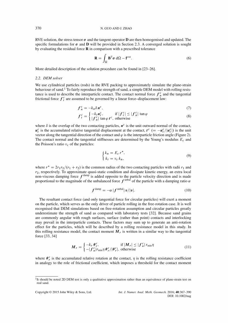
We use cylindrical particles (rods) in the RVE packing to approximately simulate the plane-strainbehaviour of sand.‡ To fairly reproduce the strength of sand, a simple DEM model with rolling resis-tance is used to describe the interparticle contact. The contact normal force f cn and the tangentialfrictional force f ct are assumed to be governed by a linear force–displacement law:
f cn D "knı nc ; (7)
f ct D²"ktuct ; if jf ct j # jf cnj tan'jf cnj tan' tc ; otherwise (8)
where ı is the overlap of the two contacting particles, nc is the unit outward normal of the contact,uct is the accumulated relative tangential displacement at the contact, tc .D "uct =juct j/ is the unitvector along the tangential direction of the contact and ' is the interparticle friction angle (Figure 2).The contact normal and the tangential stiffnesses are determined by the Young’s modulus Ec andthe Poisson’s ratio "c of the particles:
²kn D Ec r!;kt D "c kn;
(9)
where r! D 2r1r2=.r1 C r2/ is the common radius of the two contacting particles with radii r1 andr2, respectively. To approximate quasi-static condition and dissipate kinetic energy, an extra localnon-viscous damping force f damp is added opposite to the particle velocity direction and is madeproportional to the magnitude of the unbalanced force f unbal of the particle with a damping ratio ˛
f damp D "˛ jf unbalj v=jvj: (10)
The resultant contact force (and only tangential force for circular particles) will exert a momenton the particle, which serves as the only driver of particle rolling in the free-rotation case. It is wellrecognised that DEM simulations based on free-rotation assumption and circular particles greatlyunderestimate the strength of sand as compared with laboratory tests [32]. Because sand grainsare commonly angular with rough surfaces, surface (rather than point) contacts and interlockingmay prevail in the interparticle contacts. These factors may sum up to generate an anti-rotationeffect for the particles, which will be described by a rolling resistance model in this study. Inthis rolling resistance model, the contact moment M r is written in a similar way to the tangentialforce [33, 34]
M r D²"kr "cr ; if jM r j # jf cnj rmin#"jf cnjrmin#"
cr=j"cr j; otherwise (11)
where "cr is the accumulated relative rotation at the contact, # is the rolling resistance coefficientin analogy to the role of frictional coefficient, which imposes a threshold for the contact moment
‡It should be noted 2D DEM test is only a qualitative approximation rather than an equivalence of plane-strain test onreal sand.
MULTISCALE INSIGHTS INTO CLASSICAL GEOMECHANICS PROBLEMS 371
Figure 2. Illustration of the contact model in discrete element method accounting for rolling resistance.
beyond which particle rotation may be mobilised, and rmin is the minimum radius between r1 andr2. The rolling stiffness kr (Figure 2) is linked to the tangential stiffness kt and another parameterˇc through
kr D ˇc ktr1r2: (12)
Details on the implementation of the DEM model are documented in the YADE manual [35].
2.3. RVE homogenisation
The RVE packing chosen in the study contains 400 polydisperse circular (cylindrical) particles withradii ranging from 3 to 7 mm and a particle density of 2650 kg/m3. A thickness of 0.1 m is assumedfor the packing to maintain the stress measurement in pressure unit (i.e. force over area). Periodicboundary conditions are applied to both dimensions of the packing. The homogenised stress tensorof the packing is obtained from the Love formula
! D 1
V
XNc
dc ˝ f c ; (13)
where V is the volume of the RVE packing, Nc is the number of contacts within the packing, dc
is the branch vector connecting the centres of the two contacting particles (Figure 2) and f c is thecontact force. Two common stress measurements – the mean effective stress p and the deviatoricstress q – can be calculated accordingly (in 2D)
8<ˆ:
p D 1
2tr! ;
q Dr1
2s W s;
(14)
where s is the deviatoric stress tensor. The strain field is interpreted from the FEM solution, that is,the gradient of the displacement ru
where compression is taken as positive so a minus sign is present. The volumetric strain "v and thedeviatoric strain "q can then be calculated (in 2D)
´"v D tr ";
"q Dp2 e W e;
(16)
where e is the deviatoric strain tensor. Note that the displacement gradient ru will be applied aslocal boundary conditions for the DEM simulations to deform the RVE packing. In addition to strain,it indeed includes an overall rotation! D .rTu"ru/=2 as well to accommodate large deformationin strain localisation problems. The tangent operator needed to assemble the FEM stiffness matrixis given based on the uniform strain assumption [36–38]
D D 1
V
XNc
.kn nc ˝ dc ˝ nc ˝ dc C kt tc ˝ dc ˝ tc ˝ dc/: (17)
The rank-four tensor D can be written in the matrix form D (e.g. via Voigt notation) to be used inEquation 4. Note also that the interparticle rolling stiffness has no effect in calculating the tangentoperator and the stiffness matrix, as only Cauchy stress is used (Equation 13). If the couple stressis considered, for example because of the interparticle contact moments [39], the rolling stiffnessneeds to be properly incorporated into Equation 17.
3. RETAINING WALL
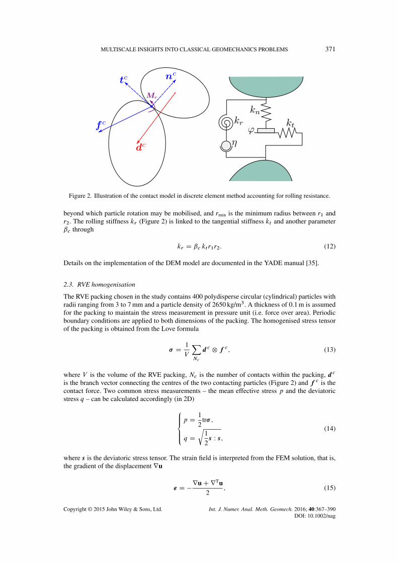
The model set-up of the retaining wall problem follows similarly that presented in [15, 40]. Adomain of 0.4 m in length and 0.2 m in depth is modelled. A rigid retaining wall with the heightof h D 0:17m is positioned at the right side of the backfill soil. A uniformly distributed surchargeqs D 20 kPa is applied on the top surface of the backfill soil. The surface of the retaining wall isassumed rough (no relative vertical displacement between wall and soil) under three wall move-ment modes (translation and rotation about the top and the bottom), and another special case withsmooth wall (no shear stress at the interface between wall and soil) is considered for the translationmode (Figure 3(a)). The soil domain is discretised by a FEM mesh of 40$ 20 eight-node quadrilat-eral elements with reduced integration (four Gauss points) as shown in Figure 3(a). The quadraticelement adopted here is found helpful to eliminate the pathological dependence on mesh density ofFEM solutions.§ The reduced integration can efficiently save the computational cost and meanwhileprovide accurate results compared with the full integration [26]. With all Gauss points counted, thesimulation involves 3200 RVE packings containing a total of 1.28 million particles for each iteration.With parallelisation on an HP SL230 Gen8 (Hewlett-Packard, Palo Alto, California, USA) server(2 $ 8-core 2.6 GHz CPU), each test in this section costs 10 to 15 h. Three different modes of wallmovement are considered under both passive and active failure conditions, which are illustrated inFigure 3(b). All RVE packings are first anisotropically consolidated to a state with a vertical stress(in x1 direction) of $v0 D 20 kPa and a horizontal stress (in x0 direction) of $h0 D 10 kPa, that is,the at-rest lateral earth pressure coefficient assumed K0 D $h0=$v0 D 0:5 and initial void ratio ofe0 D 0:182. The RVEs are then assigned to their respective Gauss points of the FEM mesh. Thisleads to an initially uniform domain. Gravity is neglected in the simulation.
3.1. DEM model and RVE effective friction angle
The microscopic parameters in the DEM model for the retaining wall problem are summarised inTable I. Similar parameters have been used in previous studies [41]. For practical interpretation inengineering applications, it is usually more convenient to use a macroscopic measurement such asthe effective friction angle '0 as frequently used in a Mohr–Coulomb criterion. Due to the non-linear
§The insensitivity of the result to the mesh density using quadratic elements is observed from additional biaxialcompression tests, which are not presented here to avoid distraction of focus.
MULTISCALE INSIGHTS INTO CLASSICAL GEOMECHANICS PROBLEMS 373
Figure 3. Model set-up on the simulation of retaining wall: (a) mesh and boundary conditions and (b) threemodes of wall movement to trigger either passive or active failure condition in the backfill soil.
Table I. Parameters for the DEM model usedin the retaining wall problem.
Ec (MPa) "c ˇc ' (ı) # ˛
300 0.3 1.0 33 0.3 0.1
DEM, discrete element method.
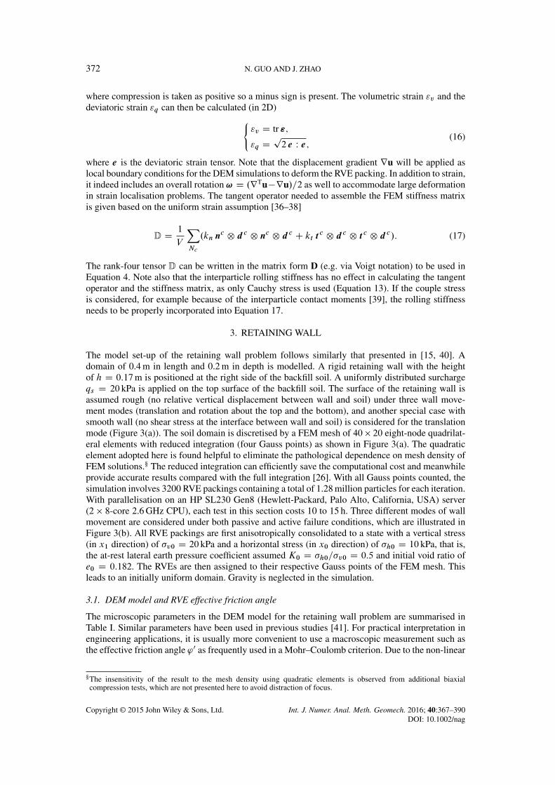
Figure 4. Estimation of the macroscopic effective friction angle of the representative volume element for theretaining wall problem.
nature in the material response, '0 is not a constant under shearing but will undergo steady changesrelated closely to the softening or hardening processes depending on the initial condition and theloading path.
To estimate the effective friction angle '0, drained biaxial compression tests were performed onthe RVE packing under two different confining pressure levels, $3 D 10 and 20 kPa, respectively.The peak stress state (failure) points were extracted from the two tests to plot their correspondingMohr’s circles as shown in Figure 4. The effective friction angle is then approximately estimatedfrom the envelope of the two circles as '0 % 47ı (assume zero cohesion). The value is relativelylarge and may correspond to some gravel materials or very dense sands [42].
3.2. Lateral earth pressure coefficient
The evolution of the lateral earth pressure coefficient, defined as the lateral earth pressure $h exertedon the wall surface normalised by the vertical stress ($v D qs D 20 kPa), against the average walldisplacement Nu (equivalent to the displacement at the centre of the wall; Figure 3(a)) normalised by
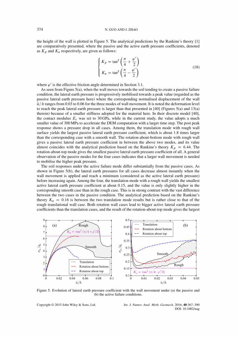
the height of the wall is plotted in Figure 5. The analytical predictions by the Rankine’s theory [1]are comparatively presented, where the passive and the active earth pressure coefficients, denotedas Kp and Ka respectively, are given as follows:
8<ˆ:
Kp D tan2"%
4C '0
2
#
Ka D tan2"%
4" '
0
2
# (18)
where '0 is the effective friction angle determined in Section 3.1.As seen from Figure 5(a), when the wall moves towards the soil tending to create a passive failure
condition, the lateral earth pressure is progressively mobilised towards a peak value (regarded as thepassive lateral earth pressure here) where the corresponding normalised displacement of the wallNu=h ranges from 0.03 to 0.06 for the three modes of wall movement. It is noted the deformation levelto reach the peak lateral earth pressure is larger than that presented in [40] (Figures 5(a) and 13(a)therein) because of a smaller stiffness adopted for the material here. In their discrete model [40],the contact modulus Ec was set to 30 GPa, while in the current study, the value adopts a muchsmaller value of 300 MPa to accelerate the DEM computation with a larger time step. The post peakresponse shows a pressure drop in all cases. Among them, the translation mode with rough wallsurface yields the largest passive lateral earth pressure coefficient, which is about 1.8 times largerthan the corresponding case with a smooth wall. The rotation-about-bottom mode with rough wallgives a passive lateral earth pressure coefficient in between the above two modes, and its valuealmost coincides with the analytical prediction based on the Rankine’s theory Kp D 6:44. Therotation-about-top mode gives the smallest passive lateral earth pressure coefficient of all. A generalobservation of the passive modes for the four cases indicates that a larger wall movement is neededto mobilise the higher peak pressure.
The soil responses under the active failure mode differ substantially from the passive cases. Asshown in Figure 5(b), the lateral earth pressures for all cases decrease almost instantly when thewall movement is applied and reach a minimum (considered as the active lateral earth pressure)before increasing again. Among the four, the translation mode with a rough wall yields the smallestactive lateral earth pressure coefficient at about 0.15, and the value is only slightly higher in thecorresponding smooth case than in the rough case. This is in strong contrast with the vast differencebetween the two cases in the passive condition. The analytical prediction based on the Rankine’stheory Ka D 0:16 is between the two translation mode results but is rather close to that of therough translational wall case. Both rotation wall cases lead to bigger active lateral earth pressurecoefficients than the translation cases, and the result of the rotation-about-top mode gives the largest
Figure 5. Evolution of lateral earth pressure coefficient with the wall movement under (a) the passive and(b) the active failure conditions.
MULTISCALE INSIGHTS INTO CLASSICAL GEOMECHANICS PROBLEMS 375
of all. These observations are indeed consistent with the FEM simulations reported in [15, 40] basedon a micropolar hypoplastic sand model, where the model parameters had been calibrated against theexperimental data on Karlsruhe sand. The different observations of lateral earth pressure evolution indifferent failure modes with different wall movements signify different progressive failure patternsand different underlying micromechanical mechanisms in the backfill soil, which are examined indetail in the sequel.
3.3. Shear-zone pattern
3.3.1. Passive failure. The apparent post-peak drop of lateral pressure in Figure 5(a) in each case isaccompanied with the occurrence of well-developed shear band(s) in the backfill soil. Towards theend of the loading, stabilised shear zones are observed. Figure 6 presents the shear-zone patterns,in terms of the accumulated shear strain "q and the void ratio e, at the end of wall movement in thepassive condition. For the case of translation mode with a rough wall (Figure 6(a)), the shear zones
Figure 6. Contours of accumulated shear strain (left panel) and void ratio (right panel) for different failuremodes under the passive condition.
depict two slip lines. The primary slip line consists of a spiral curve emanating from the bottom ofthe wall and a straight line developing towards the top surface of the backfill soil. The secondaryslip line initiates from the top of the wall extending towards the primary one at the connecting pointof the spiral segment and the straight line segment where it is intersected and cannot extend furtherdown. Shear strains and volume dilation are less intense in the second shear zone than in the first.Notably, the second slip line essentially splits the soil body above the first one into two largely rigidtriangle wedges with apparently different kinematic characteristics. The wedge bounded by the twolines and the wall features a roughly horizontal displacement, while the one above the two slip linesmoves mainly upwards.
Interestingly, the use of a smooth wall for the same translation mode leads to a single localisedshear zone only, which is a roughly straight line (Figure 6(b)). The soil wedge above the shear zonemoves up-leftwards during the loading. Apparently, the constraint of wall on the vertical move-ment of adjacent soil results in the different observations in the rough and the smooth wall cases.Rankine’s passive lateral earth pressure theory gives a theoretical angle of the passive failure slipline with respect to the horizontal plane of %=4 " '0=2 % 21:5ı. By comparing with two straightlines in the rough and the smooth wall cases, it is found the smooth wall case yields a very closevalue, which is measured as 23:5ı, while the rough wall case gives a much higher inclination angleof the slip line, which is about 35ı. The boundary condition (the rough wall assumption) and thelimited domain width could possibly attribute to this.
The rotation-about-bottom mode leads to two relatively short shear zones radiating from the topof the wall, with the higher one resembling the secondary shear line in the translation mode with arough wall (Figure 6(c)). For the case of rotation about top (Figure 6(d)), the slip line is shown tobe a spiral curve developing from the bottom of the wall towards the top surface of the backfill soil.
It is interesting to compare the current multiscale model predictions of the shear-zone patternsunder the passive failure with those experimental observations on an initially dense backfill soilusing X-ray and digital image correlation techniques reported in [40] (Figures 1 and 3 therein). Intheir experiments, the translational mode with a rough wall shows a similar double-shear-zone pat-tern – one distinct curvilinear shear zone starting from the heel of the wall to the free surface of thebackfill soil accompanied by a weak secondary shear zone propagating from the wall top. Similarly,they observed a single curved shear zone developed from the heel of the wall to the soil surface forthe rotation-about-top mode. The major difference between the current study and the experimen-tal result in [40] lies in the rotation-about-bottom mode. Instead of two radially penetrating shearzones starting from the top of the wall as observed here, multiple parallel curved shear zones wereobserved near the top of the wall in [40]. The difference may be caused by the different materialproperties as the modelled soil here has a softer response than that used in the experiment (Figure 5).It could also be attributable to the boundary condition because the soil–wall interaction is muchsimplified in the present study.
In addition to the contours of shear strain and void ratio, the distribution of average particlerotation also serves as a good indicator of the shear zone in strain localisation problems [26]. Bothexperimental [43] and DEM studies [44] show that pronounced particle rotations take place insidelocalised shear strain regions. By virtue of the hierarchical multiscale method, the average particlerotation can be quantified for any material point in the continuum field from its underlying RVEsimulation. Here, the average particle rotation N& over an RVE packing is defined as
N& D 1
Np
XNp
&p; (19)
where &p is the accumulated rotation of an individual particle where anti-clockwise rotation istreated as positive. The contours of N& for the passive failure cases are shown in Figure 7. It is notsurprising that the concentrated bands showing large particle rotations coincide well with thoseexhibiting large shear strains and dilation. For the translation failure mode with a rough wall(Figure 7(a)), the material points inside the primary shear zone experience anti-clockwise rota-tions at large, while those inside the secondary shear zone undergo clockwise rotations. For thetranslation failure mode using a smooth wall (Figure 7(b)) and the rotation-about-top failure mode
MULTISCALE INSIGHTS INTO CLASSICAL GEOMECHANICS PROBLEMS 377
Figure 7. Contours of accumulated average particle rotation for different failure modes under thepassive condition.
Figure 8. Contours of the stress normp! W ! for different failure modes under the passive condition.
(Figure 7(d)), large anti-clockwise particle rotations are observed within their respective shearzones. For the rotation-about-bottom failure mode (Figure 7(c)), clockwise particle rotation is dom-inant in the radiating shear zone. It is generally observed that when a shear slip line is initiated fromthe lower-right to the upper-left corner of the soil, anti-clockwise particle rotation dominates, andclockwise rotations prevail when a shear zone develops from the upper right to the lower left.
The stress distribution are also examined in Figure 8, where the stress measure employs thestress norm defined by
p! W ! . Generally, the stress intensities within the shear-localised zones
are not necessarily the maximum because of stress softening, which implies that the stress con-tour is not a good indicator for strain localisation [26]. Under the translation mode with a roughwall (Figure 8(a)), the stress is mainly concentrated inside the triangle wedge behind the wall,while the wedge above the two slip lines has a minimum stress concentration. For the smooth wall
(Figure 8(b)), the stress field is relatively homogeneous in the region above the toe of the wall. Onlythe shear zone shows a slightly smaller stress norm because of shear softening. Because of the samereason, in the two rotation modes, a translation of the stress concentration zone during the load-ing procedure is observed. In the rotation-about-bottom mode (Figure 8(c)), the stress concentrationmoves downwards with a successive development of the shear-localised regions, leading the finalstress concentration zone beneath the strain-localised zone. In contrast, the stress-concentrated zonemoves upwards in the rotation-about-top mode (Figure 8(d)) and stays above the shear-localisedzone at the final state.
3.3.2. Active failure. Figure 9 presents the shear-zone patterns for "q and e at the wall movementof Nu=h D 0:05 under the active failure condition. For the two translation modes with either a rough
Figure 9. Contours of accumulated shear strain (left panel) and void ratio (right panel) for different failuremodes under the active condition.
MULTISCALE INSIGHTS INTO CLASSICAL GEOMECHANICS PROBLEMS 379
or a smooth wall (Figure 9(a) and (b)), a similar straight line of shear zone develops in the soilin both cases, and the wall–soil interface in the rough case appears to develop certain shear strainconcentration too. The angle of the slip line with respect to the horizontal is 61ı for the rough wallcase and 65ı for the smooth wall case. Both are close to the theoretical value calculated by theRankine’s active lateral earth pressure theory: %=4C '0=2 % 68:5ı. For the rotation-about-bottommode, multiple small failure zones form a relatively large triangular wedge behind the wall, whichcan be better identified from the contour of void ratio (Figure 9(c)). When the rotation is about thetop of the wall, the shear zone depicts a thick spiral curve developing from the bottom of the walltowards the top surface of the backfill soil (Figure 9(d)). The curvature of the spiral curve is alsomuch larger than in the corresponding passive condition case.
Again, the distributions of the average particle rotation N& shown in Figure 10 are in good agree-ment with the contours of the shear strain and void ratio. Sand particles within the shear zonesgenerally undergo large clockwise rotations (negative N& ), but regions close to the rough wall sur-faces (Figures 9(a),(c)&(d)) show relatively large anti-clockwise particle rotations because of thestrong boundary constraint.
3.4. Local analyses
Featuring a major advantage, the current hierarchical multiscale approach enables us to offer cross-scale analyses for a complex BVP. The key macroscopic behaviours at important regions or positionsof the macrodomain can be better understood and interpreted by their micromechanical originsextracted from the local RVE simulations. As a demonstration, here we choose several Gauss pointsfor the cases of a rough wall under both passive and active translation modes to examine their localresponses and microstructural changes. The selected Gauss points are marked in Figures 7(a) and10(a) for the passive and active modes, respectively. They are initially located at the same height ofthe treated domain.
The evolutions of the stress ratio and the fabric anisotropy at the three Gauss points for thepassive failure condition are plotted in Figure 11(a) against the wall displacement, where the fab-ric anisotropy is defined based on the contact normal distribution inside a local RVE packing[45, 46] (in 2D)
8ˆ<ˆ:
# D 1
Nc
XNc
nc ˝ nc ;
F c D 4 $ dev#;
Fc Dr1
2F c W F c ;
(20)
where # is the fabric tensor and F c is the deviatoric fabric tensor. A multiplier of 4 is presentin calculating F c to ensure the integration of the distribution function E.'/ equal to 1, that is,R" E.'/ d' D 1, where E.'/ D Œ1CF c W .nc˝nc/(=.2%/. The scalar Fc is used to measure the
anisotropic intensity of the microstructure of the RVE packing. Figure 11(a) indicates the responsesof the three Gauss points, in terms of both stress ratio q=p and fabric anisotropy Fc , are ratherclose, as summarised in the following stages. For the stress ratio q=p, (a) it first experiences a quickdecrease at the beginning of the wall movement because of the flip of the major principal stressdirection from the vertical axis at rest to the horizontal one under the passive failure; (b) q=p regainsits strength and is then further mobilised to increase steadily until reaching a peak; and (c) afterpeak, an obvious softening in q=p is observed. The peak value of q=p for both GP A and GP C(inside the two shear zones) is about 0.7, which is consistent with that obtained from the element testin Figure 4. The wall displacement to reach the peak value for the two points ( Nu=h % 0:06) is alsoconsistent with that corresponding to the peak lateral earth pressure (rough wall, translation mode)in Figure 5(a). For GP B (outside the major shear zones), the peak q=p .% 0:63/ is slightly smalleras it undergoes a relatively small deformation; hence, its strength is not fully mobilised. The fabricanisotropy Fc increases monotonically to a peak value, at a slower pace than that of q=p, and thendepicts a softening response coinciding with the softening stage of q=p. Figure 11(b) presents the
Figure 10. Contours of accumulated average particle rotation for different failure modes under theactive condition.
Figure 11. Selected Gauss point (see Figures 7(a) and 10(a) on their locations) responses for the cases of arough wall under the translation mode: (a),(b) passive failure; (c),(d) active failure.
MULTISCALE INSIGHTS INTO CLASSICAL GEOMECHANICS PROBLEMS 381
evolutions of the volumetric strain "v at the three Gauss points. These points all experience overallcontraction at the early stage of wall movement ( Nu=h < 0:04) but diverge apparently with furtherwall movement. For GP A, which is inside the primary shear zone, its deformation is markedly large,and its dilation "v finally reaches about "0:08. However, for GP B, which is located in a region withsmall deformation, its volumetric change is rather small (less than 0.01) and the peak Fc of thispoint are also the smallest among the three points. The response of GP C, which is located inside thesecondary shear zone, is very similar to that of GP A. But the dilation of GP C is slightly larger thanthat of GP A. This is because GP A has a much larger confining pressure than GP C, which partlysuppresses the dilation of GP A and results in a smaller peak Fc for GP A than for GP C. For the twoGauss points under the active failure condition, their evolution curves are reminiscent of those froma monotonic loading test. The major principal direction of stress remains at the vertical direction.The increase of both q=p and Fc for the two points under the active failure condition is much fasterthan that under the passive one, which explains the instant decrease of active lateral earth pressureobserved in Figure 5(b). As GP D is located outside the shear-localised zone, its deformation level israther small. The peak stress ratio and the peak Fc at this point are much smaller than those of GP E,which is inside the shear zone as shown in Figure 11(c). Figure 11(d) indicates the two points beginto dilate upon wall movement without any initial contraction as in the passive failure condition.While the dilation of GP D is negligible, the dilation at GP E is rather noticeable, reaching about"0:12 at the final stage.
It is instructive to show the microstructures of these local Gauss points at the final stage( Nu=h D 0:1), which can be better visualised from the contact force chain network of the RVE pack-ings, as shown in Figure 12. For the passive failure mode, the RVE packing of GP A (inside theprimary shear zone) deforms severely. Several distinct strong force chains are observable, whichpenetrate through the RVE packing. An overall anti-clockwise rotation of the packing is also found,which is consistent with that shown in Figure 7(a). In contrast to GP A, the deformation at GP B(outside the localised zones) is rather small. The packing still retains a square shape similar to itsinitial configuration. The force chain network is relatively homogeneous compared with that at GPA. The packing of GP C (inside the secondary shear zone) also deforms significantly. However, itsstrong force chains are not that obvious as compared with GP A, suggesting the stress level (bothp and q) of GP C is much smaller than that of GP A, even though their stress ratio is close. Theoverall rotation of the packing at GP C is clockwise, which is again consistent with that observed inFigure 7(a). For all three points, the major principal direction of stress is roughly horizontal becausethe strong force chains align approximately horizontal. For the active failure case, the packing of GPD (outside the localised zone) undergoes a negligibly small deformation as can be observed fromthe overall very thin force chain width in the network (Figure 12(b) left). In contrast, the deforma-tion of the packing at GP E (inside the localised region) is extremely large with several strong forcechains clearly found. Its overall clockwise rotation is significant too. However, as compared withthe passive failure cases, the force chains under the active failure condition are much thinner, indi-cating that the stress level at the active failure condition is much smaller. Again for both points, themajor principal direction of stress is roughly vertical, as observed from the alignment of their strongforce chains.
4. FOOTING
The mesh and the boundary conditions for the multiscale modelling of the footing problem areshown in Figure 13 where the mesh is generated using the open-source software Gmsh [47]. Onlyhalf of the domain is modelled because of the symmetry of the problem, which is discretised into2500 second-order triangular elements (each with six nodes and three Gauss points). A total of 7500RVE packings containing 3 million particles need to be handled for every iteration in the simulation.It takes around 24 h of computation on an HP SL230 Gen8 server (2 $ 8-core 2.6 GHz CPU). Thewidth of the modelled half-domain is 0.6 m and the depth 0.4 m. The half width of the footing isB=2 D 0:05m. The bottom of the domain is fixed in both directions, while the left and the rightboundaries are only constrained by the horizontal displacement but are free to move in the verticaldirection. The base of the footing can be either rough or smooth. The influence of this assumption
Figure 12. Force chain network of the selected local Gauss points (see Figures 7(a) and 10(a) on theirlocations) in the retaining wall problem at the final stage.
Figure 13. Mesh and boundary conditions for the footing problem.
MULTISCALE INSIGHTS INTO CLASSICAL GEOMECHANICS PROBLEMS 383
is marginal as will be shown. A uniform vertical settlement d will be applied on the footing byassuming the footing is perfectly rigid. A surcharge of qs D 20 kPa is uniformly applied to thesurface. Different from the retaining wall problem, all the RVE packings in the footing problem areisotropically consolidated to attain a mean effective stress of 20 kPa before settlement is applied tothe footing. The initial void ratio for the uniform domain is e0 D 0:187. Again gravity is neglectedin the simulation.
4.1. DEM model and RVE effective friction angle
DEM parameters chosen for the footing problem are summarised in Table II. Compared with thevalues used in the retaining wall problem, an increased Young’s modulus of the particles Ec isadopted in this test to increase the macroscopic stiffness of the soil. We also decrease the interparticlefriction angle ' and the rolling resistance coefficient # to obtain a more realistic effective frictionangle '0 for fine sand. The changes to a larger stiffness (larger Ec) but a smaller shear strength(smaller ' and #) for the material make it easier to develop the general shear failure pattern in thefooting problem.
Following the same procedure described in Section 3.1, we conducted drained biaxial compres-sion tests on the RVE and drew two Mohr’s circles. The effective friction angle for the RVE isestimated as '0 % 30:5ı from the envelope of the two circles as shown in Figure 14. The inset showsthe stress–strain responses of the two drained biaxial compression tests. Note that compared withthe effective friction angle in the retaining wall problem, the fitted value here is more realistic for asandy soil [42].
4.2. Bearing capacity
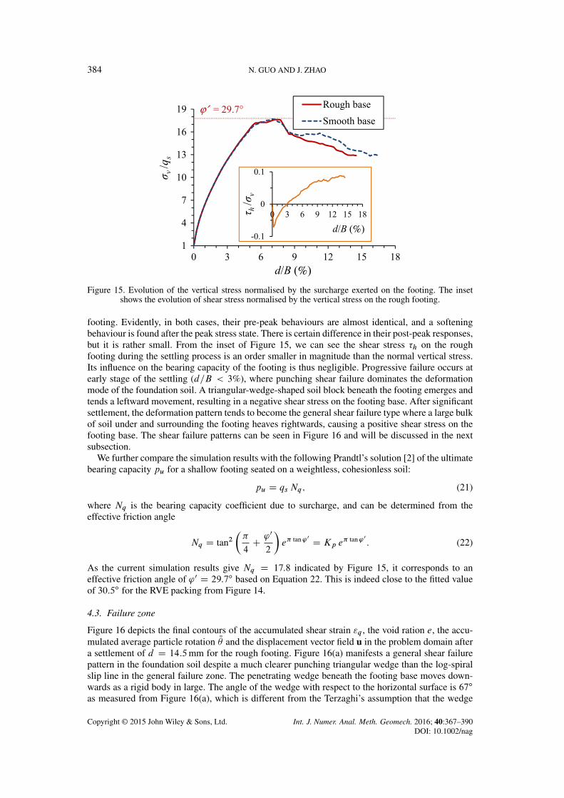
The evolution of the vertical stress $v exerted on the footing base (normalised by the surchargeqs) is plotted against the footing settlement d (normalised by the footing width B .D 0:1m/) inFigure 15 where the responses from using a rough footing are compared against those with a smooth
Table II. Parameters for the DEM model usedin the footing problem.
Ec (MPa) "c ˇc ' (ı) # ˛
800 0.5 1.0 23 0.05 0.1
DEM, discrete element method.
Figure 14. Estimation of the macroscopic friction angle of the representative volume element for thefooting problem.
Figure 15. Evolution of the vertical stress normalised by the surcharge exerted on the footing. The insetshows the evolution of shear stress normalised by the vertical stress on the rough footing.
footing. Evidently, in both cases, their pre-peak behaviours are almost identical, and a softeningbehaviour is found after the peak stress state. There is certain difference in their post-peak responses,but it is rather small. From the inset of Figure 15, we can see the shear stress )h on the roughfooting during the settling process is an order smaller in magnitude than the normal vertical stress.Its influence on the bearing capacity of the footing is thus negligible. Progressive failure occurs atearly stage of the settling (d=B < 3%), where punching shear failure dominates the deformationmode of the foundation soil. A triangular-wedge-shaped soil block beneath the footing emerges andtends a leftward movement, resulting in a negative shear stress on the footing base. After significantsettlement, the deformation pattern tends to become the general shear failure type where a large bulkof soil under and surrounding the footing heaves rightwards, causing a positive shear stress on thefooting base. The shear failure patterns can be seen in Figure 16 and will be discussed in the nextsubsection.
We further compare the simulation results with the following Prandtl’s solution [2] of the ultimatebearing capacity pu for a shallow footing seated on a weightless, cohesionless soil:
pu D qs Nq; (21)
where Nq is the bearing capacity coefficient due to surcharge, and can be determined from theeffective friction angle
Nq D tan2"%
4C '0
2
#e# tan'0 D Kp e# tan'0 : (22)
As the current simulation results give Nq D 17:8 indicated by Figure 15, it corresponds to aneffective friction angle of '0 D 29:7ı based on Equation 22. This is indeed close to the fitted valueof 30:5ı for the RVE packing from Figure 14.
4.3. Failure zone
Figure 16 depicts the final contours of the accumulated shear strain "q , the void ration e, the accu-mulated average particle rotation N& and the displacement vector field u in the problem domain aftera settlement of d D 14:5mm for the rough footing. Figure 16(a) manifests a general shear failurepattern in the foundation soil despite a much clearer punching triangular wedge than the log-spiralslip line in the general failure zone. The penetrating wedge beneath the footing base moves down-wards as a rigid body in large. The angle of the wedge with respect to the horizontal surface is 67ı
as measured from Figure 16(a), which is different from the Terzaghi’s assumption that the wedge
MULTISCALE INSIGHTS INTO CLASSICAL GEOMECHANICS PROBLEMS 385
Figure 16. Contours of (a) accumulated shear strain, (b) void ratio, (c) accumulated average particle rotationand (d) displacement field for the footing problem.
angle is equal to the effective friction angle '0. According to some experimental data, Vesic [48]concluded that the wedge corresponds to the Rankine’s active failure zone and modified the angleto %=4C '0=2 % 60:25ı. The wedge angle from the simulation is also slightly larger than the valuemodified after Vesic but already close enough. One possible reason is that the current deformationpattern is more dominated by the punching shear failure beneath the footing, while the shear slipzones in the general failure mode are relatively weak.
The general shear failure pattern is more clearly seen from the void ratio contour as shown inFigure 16(b). From the figure, it is apparent that a third shear slip line emerges from the footingedge down-rightwards and is intercepted by the general failure slip line. The general shear failureslip line can be approximately described by a log-spiral curve as follows:
r D r0 e tan'0 ; (23)
where measures the direction (with regard to the vertical axis) of the line connecting the centre ofthe footing and the point located on the log-spiral curve, r is the length of the line and r0 is the linelength when D 0ı and is also the height of the inverted triangular wedge. Two such curves with'0 D 30:5ı and 33:5ı, respectively, are superimposed in Figure 16(b), which match the simulatedgeneral failure slip line reasonably well. The used values of the effective friction angle are close tothe fitted one for the RVE packing in Figure 14.
The contour of the accumulated average particle rotation, shown in Figure 16(c), also clearlydepicts the general shear failure pattern. Inside the punching shear zone, particles mainly rotate anti-clockwise (positive N& ), while those inside the general failure slip line rotate clockwise (negativeN& ). However, as the shear strain in the general failure slip line is much weaker than that in thepunching shear zone, the magnitude of the clockwise rotation is much smaller than that of the anti-clockwise rotation (note that the colour bar ranges from "0.1 to 0.6). Furthermore, the punching of
the triangular wedge beneath the footing and the heaving of the bulk soil beside the footing can beclearly seen from the displacement vector plot in Figure 16(d).
4.4. Local analyses
Similar to that in Section 3.4, we can further examine the local responses and the microstructuresfor some Gauss points of interest. Two Gauss points are selected whose positions are marked inFigure 16(c). GP A is located inside the shear zone of the punching wedge, and GP B is insidethe general failure spiral line. Figure 17 presents the evolutions of the stress ratio q=p, the fabricanisotropy Fc and the volumetric strain "v of the two points against the footing settlement. While thestress ratio of both points shows an increase followed by a decrease trend, the increase of q=p at GPA is much faster than that at GP B. The difference is even more appreciable for the increase of fabricanisotropy. At GP A, the change of the local structure is instant as the footing begins to settle. Thechange of the local structure at GP B is rather slow in pace. Similar trend can be observed from thedilation curves of the two points. Following a small contraction, GP A begins to dilate significantlyafter d=B D 0:03, while for GP B, an obvious dilation is not observed until d=B > 0:08. Thedifference in evolution at the two Gauss points clearly corroborates the progressive failure natureof the footing problem, that is, the local punching failure dominates before the general failure isformed at a relatively large footing settlement.
The force chain network of the two Gauss points at the final stage (d=B D 0:145) is shownin Figure 18. As can be seen, the deformation level at GP A is rather large. The RVE packingis severely distorted with a clearly overall anti-clockwise rotation. A few penetrating strong force
Figure 17. Selected Gauss point responses in the footing problem.
Figure 18. Force chain network of the selected local Gauss points in the footing problem at the final stage.
MULTISCALE INSIGHTS INTO CLASSICAL GEOMECHANICS PROBLEMS 387
chains are found inside the packing. These are in great contrast with the relatively small deformationand less-distinct force chains in the GP B case. The packing at GP B as a whole undergoes a mildclockwise rotation. The opposite rotation directions for GP A and GP B are consistent with thatobserved in Figure 16(c). The difference in the alignments of the strong force chains inside the twoRVE packings indicate the major principal stress directions at this two points are different fromeach other.
5. CONCLUDING REMARKS
The paper presented a novel computational multiscale modelling approach based on hierarchicalcoupling of FEM and DEM in application to two classical geotechnical problems – the retainingwall and the footing. This hierarchical multiscale modelling approach adopts FEM to solve thecontinuum-level BVPs and assigns DEM packings to the Gauss points of the FEM mesh to derive thelocal material responses from independent simulations. In doing so, the phenomenological natureinherent to conventional continuum modelling approaches can be avoided. It is demonstrated thismultiscale approach is capable to predict the passive and the active lateral earth pressure coeffi-cients, and the bearing capacity of shallow foundations, as well as very complicated failure patternsin these problems. The simulations compared reasonably well with available analytical solutions(which have been derived based on certain assumptions). It is not surprising because the framework,with its embedded DEM simulation at the mesoscale/microscale, could naturally incorporate thematerial nonlinearity and plasticity originated from the particle level in the continuum-scale com-putation. Further, cross-scale analyses and correlation of observations on the macroscopic failurepatterns and the strong force chain network and particle rotations confirm the validity, robustness andpredictive capability of the proposed method. Some main findings from the study are summarisedin the following.
1. To obtain the realistic macroscopic friction angle for a real sand/gravel, rolling resistanceneeds to be considered in the DEM model if simplified circular/spherical particles are usedto compensate for the particle shape effect. The effective friction angle of the material is thendetermined from the element tests on the RVE packing based on Mohr’s circles. The micro-scopic parameters in the DEM model, which are the only parameters required in the currenthierarchical multiscale approach, can be calibrated from laboratory tests on sand/gravel.
2. The numerically determined passive and active lateral earth pressure coefficients are close tothe theoretical predictions by Rankine. The assumption of a rough or a smooth wall under thetranslation mode yields very different Kp but similar Ka. While the translation mode givesthe largest Kp but the smallest Ka, the rotation-about-top mode gives the smallest Kp andthe largest Ka. The lateral earth pressure coefficients under both the passive and the activefailure conditions for the rotation-about-bottom mode lie in between the other two modes.Furthermore, the active earth pressure decreases more quickly than the increase of the passiveearth pressure, which can be explained from the local analyses of some selected Gauss points.The mobilisation of the microstructural response of the RVE packings is much slower in thepassive failure than in the active failure.
3. The shear-zone pattern for the passive failure under the translation mode with a rough wallshows two major shear bands. The primary one emerges from the heel of the wall and prop-agates towards the surface of the backfill soil. The secondary one emanates from the top ofthe wall and pierces into the soil and is intercepted by the primary one. For the correspondingsmooth wall case, there exists only one shear band depicting a look of straight line and an anglewith regard to the horizontal surface very close to the Rankine’s theoretical value for passivefailure. The shear bands for the active condition under translation mode with either a rough ora smooth wall shows a single straight line pattern with an angle with regard to the horizontalsurface close to the Rankine’s theoretical value for active failure. The simulation results showgood agreements with both experimental observations and FEM predictions [15, 16, 40].
4. The simulated ultimate bearing capacity of the shallow footing matches the Prandtl’s solutionfairly well. A general shear failure pattern is observed, where the failure zone consists of a
punching triangular wedge right beneath the footing and a shear slip line tending towards theground surface of the soil. The angle of the wedge with respect to the horizontal surface isslightly larger than the Vesic’s modification [48], that is, the angle of the Rankine’s activefailure line. The general failure slip line can be largely described by a log-spiral curve. Thelocal analyses of the two Gauss points (one inside the wedge shear zone, the other inside theslip line) indicate a progressive failure mode for the footing problem.
5. Besides the shear strain and the void ratio contours that are commonly used, the contour ofaccumulated average particle rotation proves to be an additional good indicator for the analy-sis of strain localisation. While severe particle rotations generally take place inside the shearbands, the directions of particle rotations within different shear zones could be opposite, suchas the cases of the passive failure under translation mode for the rough retaining wall and thegeneral shear failure for the footing.
The focus of the study has been placed on demonstrating the applicability of the hierarchical mul-tiscale approach in solving practical geotechnical problems. Related to the study, there are severalexploratory topics meriting continuous investigations. For example, considering the heterogeneityof geomaterials in a natural setting, it appears more reasonable if the properties of geomaterials areconsidered to be spatially random [49, 50]. By assigning different RVE packings (e.g. varying ini-tial void ratios) to the Gauss points, the influence of inherent heterogeneity of natural sand can bestudied using this approach. Besides the static problems already treated here, dynamic loading isof major interest to earthquake engineers and can be studied based on this approach with moderatemodifications as well, for example by considering viscosity in the DEM model and inertia terms inthe FEM solution. In addition, the micro–macro bridging capability of the proposed approach needsto be further explored to assist a comprehensive understanding of the physics and mechanics gov-erning the shear behaviour of granular soils. The topics listed earlier are important continuations ofthe study, which are practically tractable. Meanwhile, there are more formidable challenges pertain-ing to the multiscale approach, which may need a coordinated effort among different parties, forexample numerical modellers, experimentalists, computer scientists and physicists. The followingprovides a number of examples.
1. The hierarchical multiscale approach relies crucially on the DEM part to provide reliable,quantitative predictions, while it remains challenging to accurately calibrate the DEM modelparameters. Indeed, if the rolling resistance model or the clumped particle model is usedin the DEM, a common way of calibration remains to be curve fitting, which is essentiallyphenomenological. To overcome this obstacle, proper characterisation and modelling of theparticle shape need to be implemented in DEM. Some recent progresses have been made in thisregard, for example [51–53]. However, how to effectively implement the generated complex-shaped particles into DEM remains a bottleneck, which may need the help from computerscientists and applied mathematicians. Meanwhile, advanced particle-scale tests [54, 55] arerequired to provide essential microscopic parameters such as the contact moduli and the inter-particle friction angle for the DEM simulation. This will constitute a key step towards realapplication of the multiscale approach to geotechnical designs.
2. Inherited from the adopted conventional continuum model, the solution of the current hierar-chical multiscale approach is found dependent on element type [24] though being less sensitiveto mesh density. It is because in upscaling the Gauss point responses to the FEM, the informa-tion of the intrinsic length of the material is lost. For a problem with material softening, theBVP could be ill-posed. To tackle this issue, a simple nonlocal regularisation [56] could beemployed, which is currently examined by the authors.
3. The success of the multiscale approach depends critically on its computational efficiency. Onone hand, we may seek more computing power by virtue of the parallel structure of the frame-work; on the other hand, the computational algorithm of the approach needs to be pushed to anew level of efficiency too. For example, further effort needs to be made to find a consistenttangent operator, which can provide quadratic convergence for the Newton–Raphson iteration.
4. How to consider the presence of pore fluid in sand in the multiscale approach is another chal-lenge. A full consideration of the influence of pore fluid may require a further coupling of the
MULTISCALE INSIGHTS INTO CLASSICAL GEOMECHANICS PROBLEMS 389
DEM with another software simulating the behaviour of pore fluid, such as lattice Boltzmmanmethod or computational fluid dynamics method, for each RVE, which inevitably poses greatchallenges to the hierarchical formulation, specification of macro/micro boundary conditionand handling of the computational cost that increases by orders of magnitude.
ACKNOWLEDGEMENTS
We thank the two anonymous reviewers for their constructive comments. The second author also wishes tothank Prof. Itai Einav for suggesting the multiscale study of the footing problem during a conversation in theIWBDG 2014 conference. We acknowledge the support from Science School Computational Science Initia-tive, HKUST, for allowing us to access its HPC facility. The study was financially supported by ResearchGrants Council of Hong Kong (GRF Grant No. 623211).
REFERENCES
1. Rankine WJM. On the stability of loose earth. Philosophical Transactions of the Royal Society of London 1857;147:9–27.
2. Prandtl L. Uber die Härte plastischer Körper. Nachrichten von der Königlichen Gesellschaft der Wissenschaften,Göttingen, Math.-Phys. Klasse 1920; 1920:74–85.
3. Terzaghi K. Theoretical Soil Mechanics. Wiley: New York, 1943.4. Taylor DW. Fundamentals of Soil Mechanics. Wiley: New York, 1948.5. Drucker DC, Prager W, Greenberg HJ. Extended limit design theorems for continuous media. Quarterly of Applied
Mathematics 1952; 9:381–389.6. Prager W. The general theory of limit design. Proceedings of the 8th International Congress of Theoretical and
Applied Mechanics (Istanbul 1952), Istanbul, 1955; 65–72.7. Gutierrez M, Ishihara K. Non-coaxiality and energy dissipation in granular material. Soils and Foundations 2000;
40:49–59.8. Yu HS, Yuan X. On a class of non-coaxial plasticity models for granular soils. Proceedings of the Royal Society A
2006; 462(2067):725–748.9. Casagrande A, Carillo N. Shear failure of anisotropic materials. Proceedings of Boston Society of Civil Engineers
1944; 31:74–87.10. Arthur JRF, Menzies BK. Inherent anisotropy in a sand. Géotechnique 1972; 22(1):115–128.11. Arthur JRF, Chua KS, Dunstan T. Induced anisotropy in a sand. Géotechnique 1977; 27(1):13–30.12. Roscoe KH, Schofield AN, Wroth CP. On the yielding of soils. Géotechnique 1958; 8(1):22–53.13. Schofield AN, Wroth CP. Critical State Soil Mechanics. McGraw-Hill: London, UK, 1968.14. Vardoulakis I. Deformation of water-saturated sand: I. Uniform undrained deformation and shear band. Géotechnique
1996; 46(3):441–456.15. Nübel K, Huang W. A study of localized deformation pattern in granular media. Computer Methods in Applied
Mechanics and Engineering 2004; 193(27–29):2719–2743.16. Tejchman J. FE-analysis of patterning of shear zones in granular bodies for earth pressure problems of a retaining
wall. Archives of Hydro-Engineering and Environmental Mechanics 2004; 51(4):317–348.17. Desrues J, Viggiani G. Strain localization in sand: an overview of the experimental results obtained in Grenoble
using stereophotogrammetry. International Journal for Numerical and Analytical Methods in Geomechanics 2004;28(4):279–321.
18. Banimahd M, Woodward PK. Load-displacement and bearing capacity of foundations on granular soils using amulti-surface kinematic constitutive soil model. International Journal for Numerical and Analytical Methods inGeomechanics 2006; 30:865–886.
19. Gao Z, Zhao J. Strain localization and fabric evolution in sand. International Journal of Solids and Structures 2013;50:3634–3648.
20. Conte E, Donato A, Troncone A. Progressive failure analysis of shallow foundations on soils with strain-softeningbehaviour. Computers and Geotechnics 2013; 54:117–124.
21. Terzaghi K. Old earth pressure theories and new test results. Engineering News Record 1920; 85:632–637.22. Cundall PA, Strack ODL. A discrete numerical model for granular assemblies. Géotechnique 1979; 29(1):47–65.23. Guo N, Zhao J. A hierarchical model for cross-scale simulation of granular media. In AIP Conference Proceedings,
Vol. 1542, Yu A (ed.). AIP Publishing: Sydney, Australia, 2013; 1222–1225.24. Guo N, Zhao J. A coupled FEM/DEM approach for hierarchical multiscale modelling of granular media. Interna-
tional Journal for Numerical Methods in Engineering 2014; 99(11):789–818.25. Guo N. Multiscale characterization of the shear behavior of granular media. Ph.D. Thesis, Hong Kong, 2014.26. Zhao J, Guo N. The interplay between anisotropy and strain localisation in granular soils: a multiscale insight.
Géotechnique 2015. DOI: 10.1680/geot.14.P.184.27. Meier HA. Computational homogenization of confined granular media. Ph.D. Thesis, 2009.28. Miehe C, Dettmar J, Zäh D. Homogenization and two-scale simulations of granular materials for different
microstructural constraints. International Journal for Numerical Methods in Engineering 2010; 83:1206–1236.
29. Andrade J, Avila C, Hall S, Lenoir N, Viggiani G. Multiscale modeling and characterization of granular matter: fromgrain kinematics to continuum mechanics. Journal of the Mechanics and Physics of Solids 2011; 59:237–250.
30. Nitka M, Combe G, Dascalu C, Desrues J. Two-scale modeling of granular materials: a DEM-FEM approach.Granular Matter 2011; 13(3):277–281.
31. Nguyen TK, Combe G, Caillerie D, Desrues J. FEM " DEM modelling of cohesive granular materials: numericalhomogenisation and multi-scale simulations. Acta Geophysica 2014; 62(5):1109–1126.
32. Oda M, Konishi J, Nemat-Nasser S. Experimental micromechanical evaluation of strength of granular materials:effects of particle rolling. Mechanics of Materials 1982; 1:269–283.
33. Ishihara K, Oda M. Rolling resistance at contacts in simulation of shear band development by DEM. Journal ofEngineering Mechanics 1998; 124(3):285–292.
34. Zhao J, Guo N. Rotational resistance and shear-induced anisotropy in granular media. Acta Mechanica Solida Sinica2014; 27(1):1–14.
35. Šmilauer V, Catalano E, Chareyre B, Dorofeenko S, Duriez J, Gladky A, Kozicki J, Modenese C, Scholtès L, SibilleL, Stránský J, Thoeni K, et al. Yade reference documentation. In Yade Documentation, (1st edn), Šmilauer V. (ed.).The Yade Project, 2010.
36. Wren JR, Borja RI. Micromechanics of granular media Part II: overall tangential moduli and localization model forperiodic assemblies of circular disks. Computer Methods in Applied Mechanics and Engineering 1997; 141:221–246.
37. Kruyt N, Rothenburg L. Statistical theories for the elastic moduli of two-dimensional assemblies of granularmaterials. International Journal of Engineering Science 1998; 36:1127–1142.
38. Luding S. Micro-macro transition for anisotropic, frictional granular packings. International Journal of Solids andStructures 2004; 41:5821–5836.
39. Wensrich CM. Stress, stress-asymmetry and contact moments in granular matter. Granular Matter 2014; 16:597–608.
40. Widulinski Ł., Tejchman J, Kozicki J, Lesniewska D. Discrete simulations of shear zone patterning in sand in earthpressure problems of a retaining wall. International Journal of Solids and Structures 2011; 48:1191–1209.
41. Kozicki J, Tejchman J, Mühlhaus HB. Discrete simulations of a triaxial compression test for sand by DEM.International Journal for Numerical and Analytical Methods in Geomechanics 2014; 38:1923–1952.
42. Meyerhof GG. Penetration tests and bearing capacity of cohesionless soils. Journal of the Soil Mechanics andFoundations Division 1956; 82(1):1–19.
43. Hall SA, Bornert M, Desrues J, Pannier Y, Lenoir N, Viggiani G, Bésuelle P. Discrete and continuum analysisof localised deformation in sand using X-ray $CT and volumetric digital image correlation. Géotechnique 2010;60(5):315–322.
44. Bardet JP, Proubet J. A numerical investigation of the structure of persistent shear bands in granular media.Géotechnique 1991; 41(4):599–613.
45. Satake M. Fabric tensor in granular materials. In IUTAM Symposium on Deformation and Failure of GranularMaterials. A.A. Balkema: Delft, 1982; 63–68.
46. Oda M. Fabric tensor for discontinuous geological materials. Soils and Foundations 1982; 22(4):96–108.47. Geuzaine C, Remacle JF. Gmsh: a 3-D finite element mesh generator with built-in pre- and post-processing facilities.
International Journal for Numerical Methods in Engineering 2009; 79:1309–1331.48. Vesic AS. Analysis of ultimate loads of shallow foundations. Journal of the Soil Mechanics and Foundations Division
1973; 99(1):45–73.49. Andrade JE, Baker JW, Ellison KC. Random porosity fields and their influence on the stability of granular media.
International Journal for Numerical and Analytical Methods in Geomechanics 2008; 32:1147–1172.50. Chen Q, Seifried A, Andrade JE, Baker JW. Characterization of random fields and their impact on the mechanics of
geosystems at multiple scales. International Journal for Numerical and Analytical Methods in Geomechanics 2012;36:140–165.
51. Mollon G, Zhao J. Fourier-Voronoi-based generation of realistic samples for discrete modelling of granular materials.Granular Matter 2012; 14:621–638.
52. Mollon G, Zhao J. Generating realistic 3D sand particles using Fourier descriptors. Granular Matter 2013; 15:95–108.
53. Mollon G, Zhao J. 3D generation of realistic granular samples based on random fields theory and Fourier shapedescriptors. Computer Methods in Applied Mechanics and Engineering 2014; 279:46–65.
54. Hall SA, Wright J, Pirling T, Andò E, Hughes DJ, Viggiani G. Can interparticle force transmission be identified insand? First results of spatially-resolved neutron and X-ray diffraction. Granular Matter 2011; 13:251–254.
55. Senetakis K, Coop MR, Todisco MC. The inter-particle coefficient of friction at the contacts of Leighton Buzzardsand quartz minerals. Soils and Foundations 2013; 53:746–755.
56. Bažant Z, Jirásek M. Nonlocal integral formulations of plasticity and damage: survey of progress. Journal ofEngineering Mechanics 2002; 128:1119–1149.


![A stochastic mixed finite element heterogeneous multiscale ...multiscale elliptic problems with the conforming linear FEM (FeHMM) [20– 22]. The method was analyzed in a series of](https://static.documents.pub/doc/80x56/60df0481e7ce0b727f4de3bd/a-stochastic-mixed-inite-element-heterogeneous-multiscale-multiscale-elliptic.jpg)


