Multivariate density estimation and its applications

Wing Hung WongStanford University

June 2014, Madison, Wisconsin. Conference in honor of the 80th birthday of Professor Grace Wahba

Estimate the function…Put prior on function space…Use RKHS, splines, approximation theory….

Lessons I learned in graduate school:

A 3‐dimensional density function from flow cytometry

Mass cytometry: replace fluorescent labels with elemental labels

Mass-spectra

Holmium164.93031 amu

The Bayesian nonparametric problem

• x1 , x2 , …xn are independent r.v. on a space Ω• Their distribution Q is unknown but assumed to be drawn from a prior distribution π.

• Our tasks: Prior construction, posterior computation

• Want this to work well when Ω is of moderately high dimension, e.g. 5‐50

π(Q) Q(X) → Pr( Q, X) → Pr (Q | X ) → Pr (g(Q))

Ferguson’s criteria (1973)• Support of the prior should be large• The posterior should be tractable

Dirichlet process prior satisfies Ferguson’s conditions.

However, under this prior the random distribution Q does not possess a density

Density is useful in many applications

• Anomaly detection• Classification

• Compression• Probabilistic networks• Image analysisand more

We want to define a prior on the space of simple density functions:

f(x) = ∑ ci IAi(x)

To reduce complexity of this space, assume that Ω=A1 U A2…. U Am is a recursive partition

A

A12

A11

A1221

A1222

A21

A22

In general, Ajk = kth part of the jth way to partition A

Recursive partitions:

Level 1

Level 2

Q is uniform within A

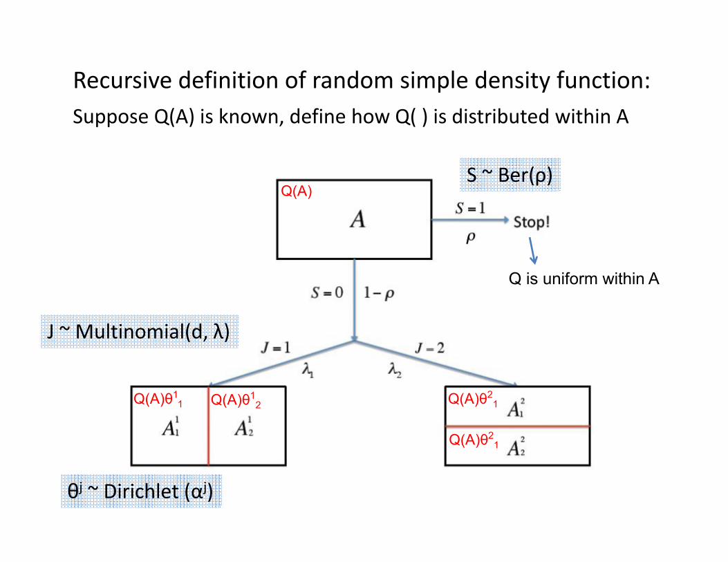
Recursive definition of random simple density function:Suppose Q(A) is known, define how Q( ) is distributed within A

Q(A)

Q(A)θ11 Q(A)θ1

2 Q(A)θ21

Q(A)θ21

S ~ Ber(ρ)

J ~ Multinomial(d, λ)

θj ~ Dirichlet (αj)

Density on partitions of finite depth

• Suppose we have drawn Q(k) supported on a partition composing of regions up to level k

• For each region not yet stopped, repeat the partitioning process

• This gives a random distribution Q(k+1) with a density q(k+1) that is piecewise constant on a partition with regions up to level k+1

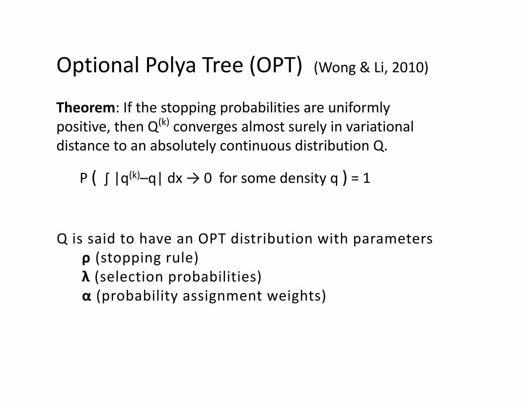
Q is said to have an OPT distribution with parameters ρ (stopping rule) λ (selection probabilities) α (probability assignment weights)

P ( ∫ |q(k)–q| dx → 0 for some density q ) = 1

Optional Polya Tree (OPT) (Wong & Li, 2010)

Theorem: If the stopping probabilities are uniformly positive, then Q(k) converges almost surely in variationaldistance to an absolutely continuous distribution Q.

2) π( Q | x1, ..xn ) is also OPT with parametersρ (x1, ..xn ), λ (x1, ..xn ), α (x1, ..xn ),

computable in finite time

OPT prior satisfies Ferguson’s criteria

1) Any L1 ball has positive prior probability

Q(A)

Q(A)θ11 Q(A)θ1

2 Q(A)θ21

Q(A)θ21

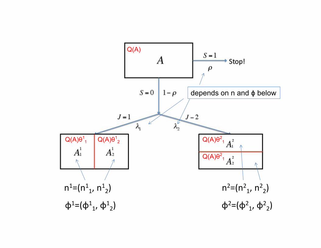
n1=(n11, n12) n2=(n21, n22)

φ1=(φ11, φ1

2) φ2=(φ21, φ2

2)

depends on n and ϕ below

Computation of Φ(A) by recursion

where

Recursion ends when A has either 0 or 1 data points.

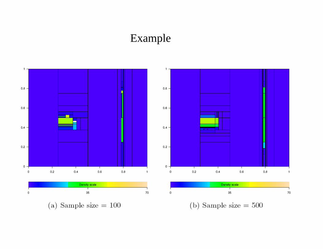
Example

Example (continued)

2nd approach: build up partition sequentially

v

Given t, want to define a posterior score for the partition directly

…

… …

t=2

t=3

t=4

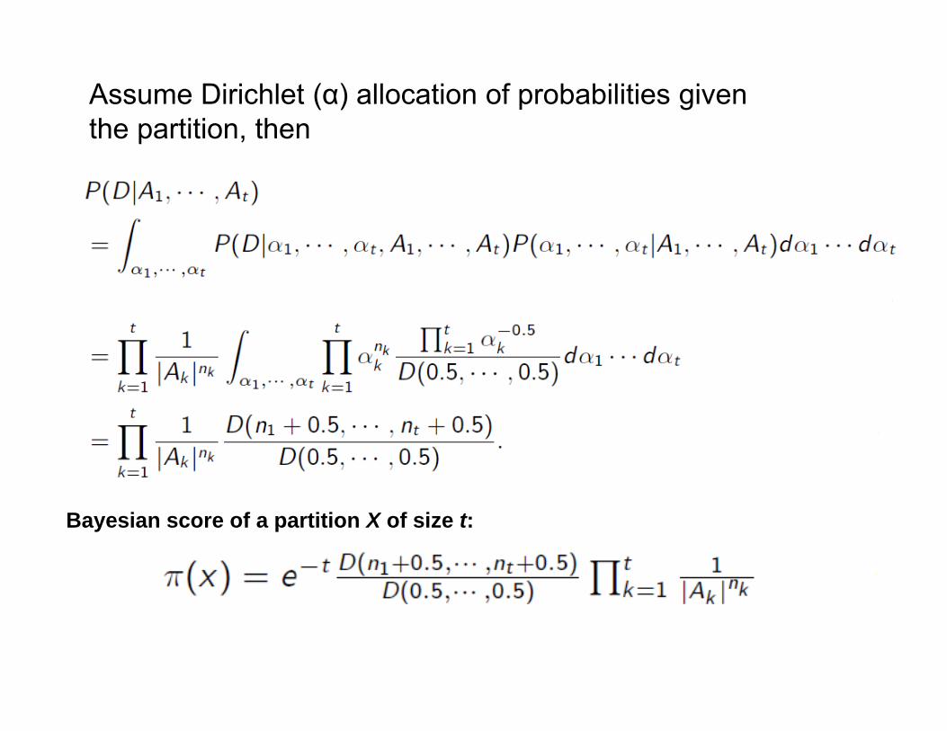
Bayesian score of a partition X of size t:

Assume Dirichlet (α) allocation of probabilities given the partition, then

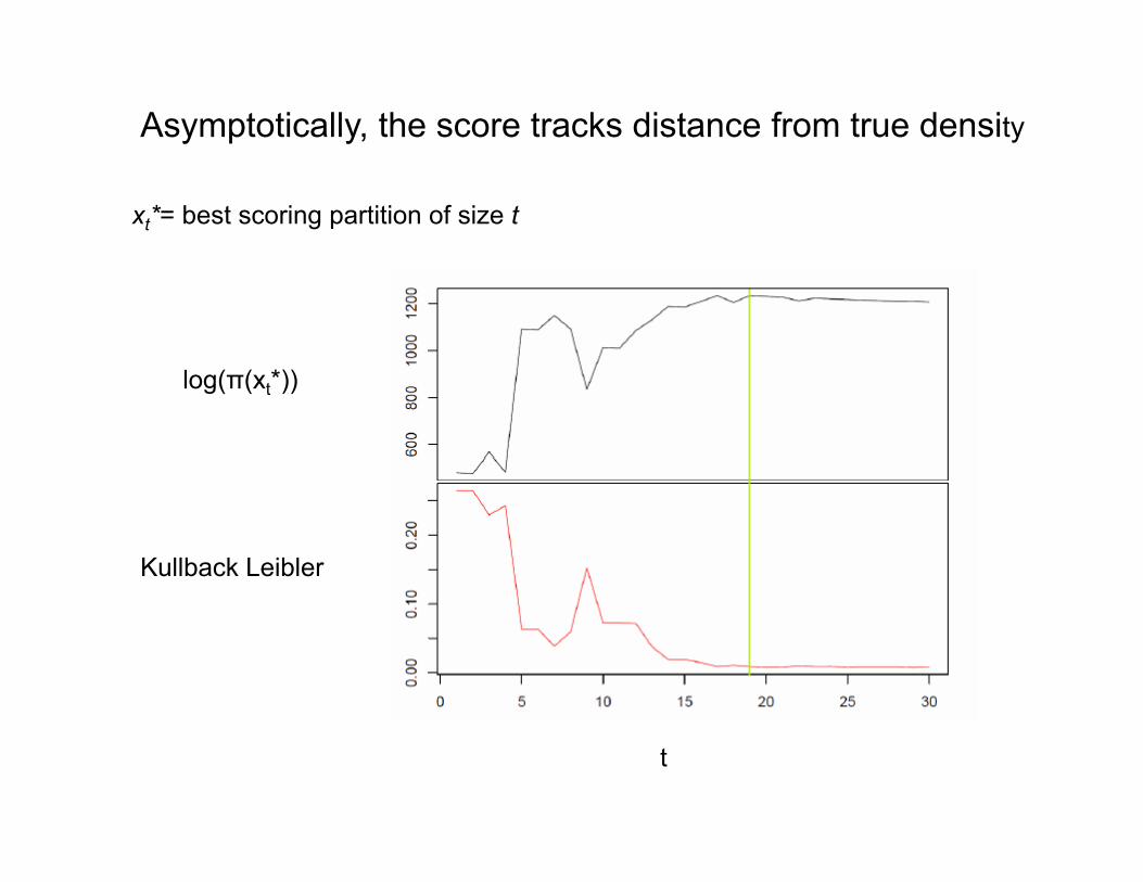
log(π(xt*))

Kullback Leibler

xt*= best scoring partition of size t

t

Asymptotically, the score tracks distance from true density

Sequential importance sampling

v

Cut 1 Cut 2 Cut 3

v

Partition 1

Partition 2

vPartition 3

vPartition 4 v

v v

Partition Sample

Generate cuts randomly

M

w1 w1

w2

w3

w4

w2

w3

w4

t

k

n

k

ttt

k

ADnnDey

121

21

21

121 1

,,,,)ˆ(

How to choose the proposal density?

)|().....|()()( 1121,.....2,1 ttttttt yyyyyyyy

)|().....|()()( 112211,.....2,1 ttttt yyyyyyyyq

feasibleinfeasible

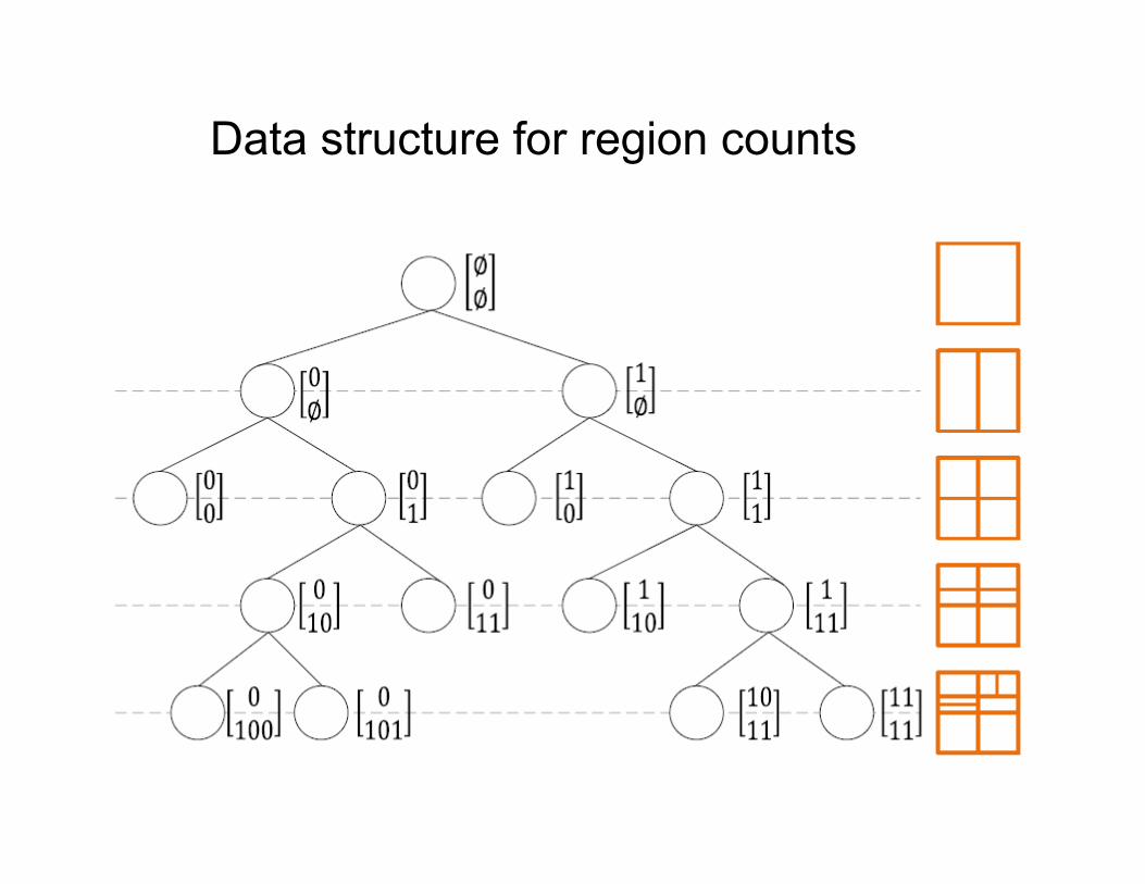
Data structure for region counts

Counting can be accelerated by hardware

• Intel(R) Xeon(R) CPU E5640 @ 2.67GHz

• GeForce GTX 680– 1536 CUDA cores (8*192) @ 1.08GHz– 512KB L2– 2G RAM– Memory clock rate: 3GHz– Memory bus width: 256‐bit– Bandwidth: 150GB/s

Experiment result (CountEngine)

• Partition = 300, Cut = 1000

Dim_# of data CPU GPU Speedup

32_10^5 33375.40 18.56 1798.54

32_10^6 316794.00 28.82 10992.20

64_10^5 113327.00 24.59 4609.34

64_10^6 1086660.00 39.38 27593.51

128_10^5 438960.00 34.19 12837.45

128_10^6 NA 57.50 NA

Resampling:

Comparison with Kernel Density Estimate

Sample n points from a D-dim distribution:

Results:

Estimate of conditional density in 7 dimension

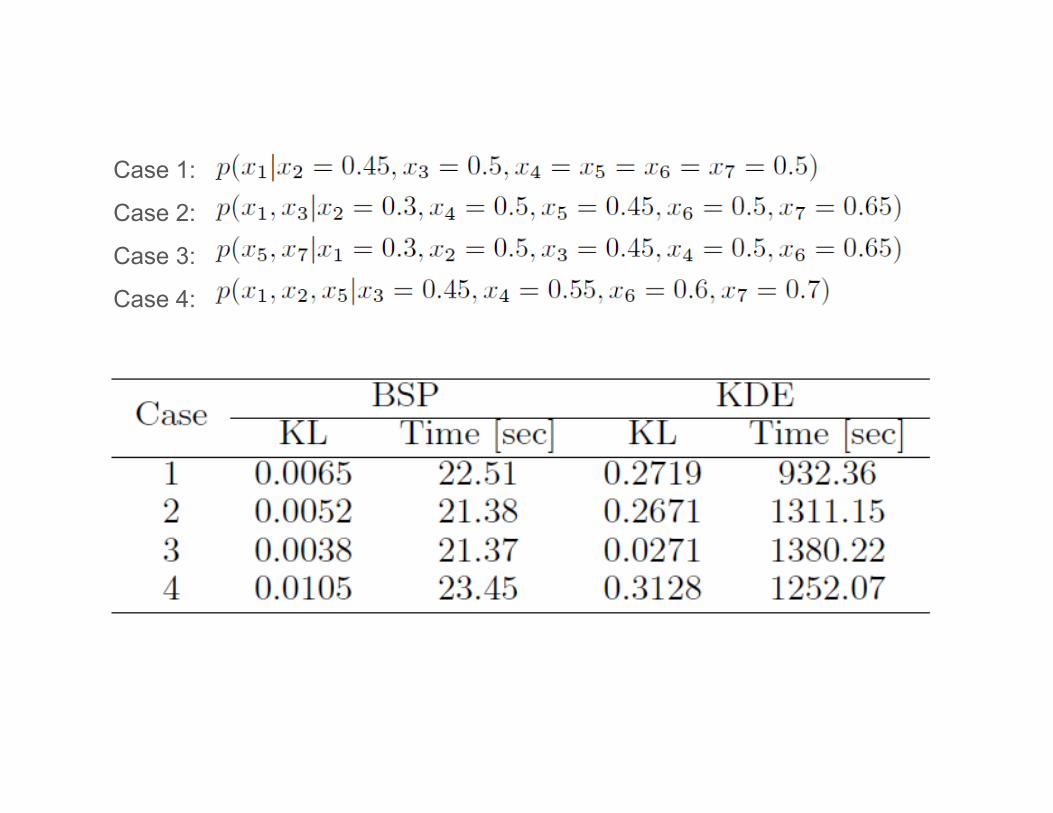
Case 1:

Case 2:

Case 3:

Case 4:

Density estimation is a building block for other statistical methods.

Classification: 1) Estimate class density fi(x) for classes 1, …k

2) Use Bayes classifier: p(i|x) ~ αi fi(x)

MAGIC data: 10 dimension, 12,000 cases, 7,000 controls

Letter data: 16 dimension, 26 classes, n=16,000 within class

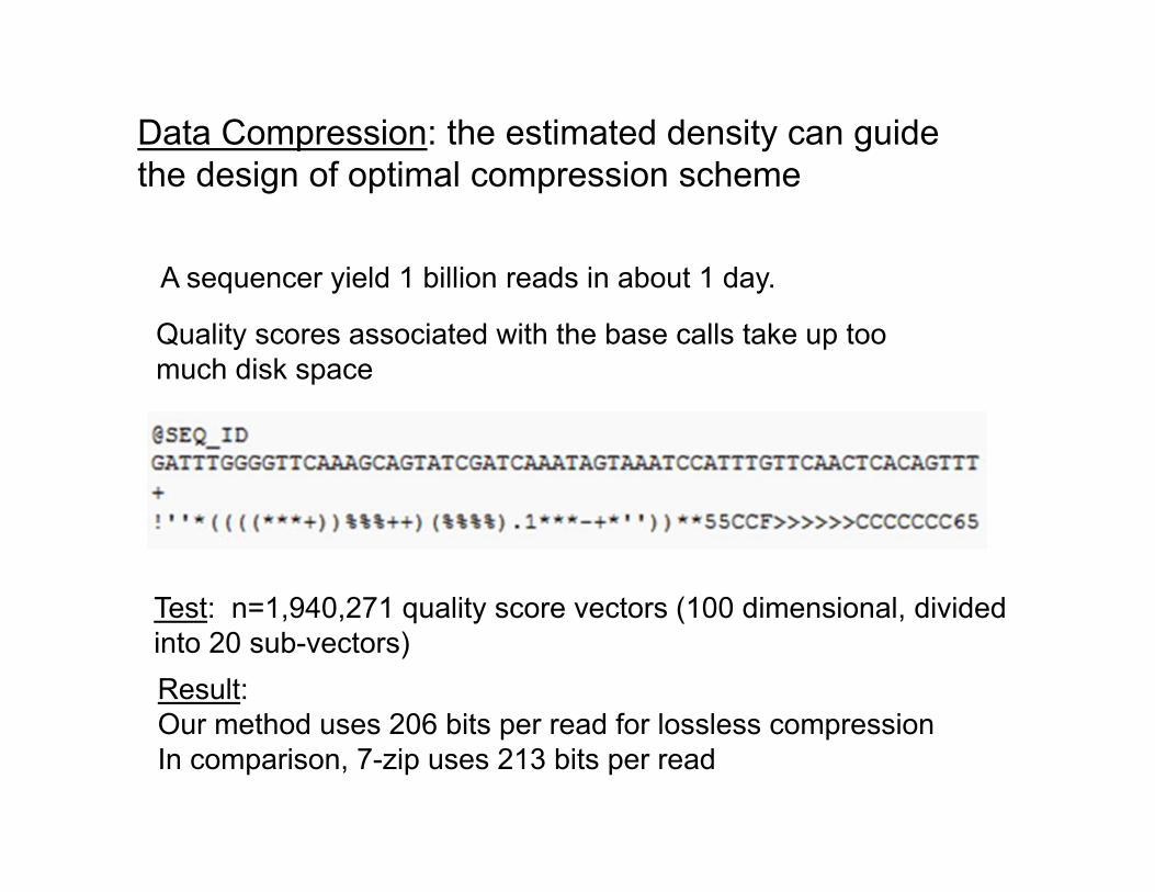
A sequencer yield 1 billion reads in about 1 day.

Quality scores associated with the base calls take up too much disk space

Test: n=1,940,271 quality score vectors (100 dimensional, divided into 20 sub-vectors) Result:Our method uses 206 bits per read for lossless compressionIn comparison, 7-zip uses 213 bits per read

Data Compression: the estimated density can guide the design of optimal compression scheme

Contour plot of the energy function of a 2D density with seven modes

Sub-level tree of energy(log-density)

Visualization of information

density CD11b

CD4TCR-b

B220

CD8

Sublevel tree of bone marrow data (n=2,000,000)

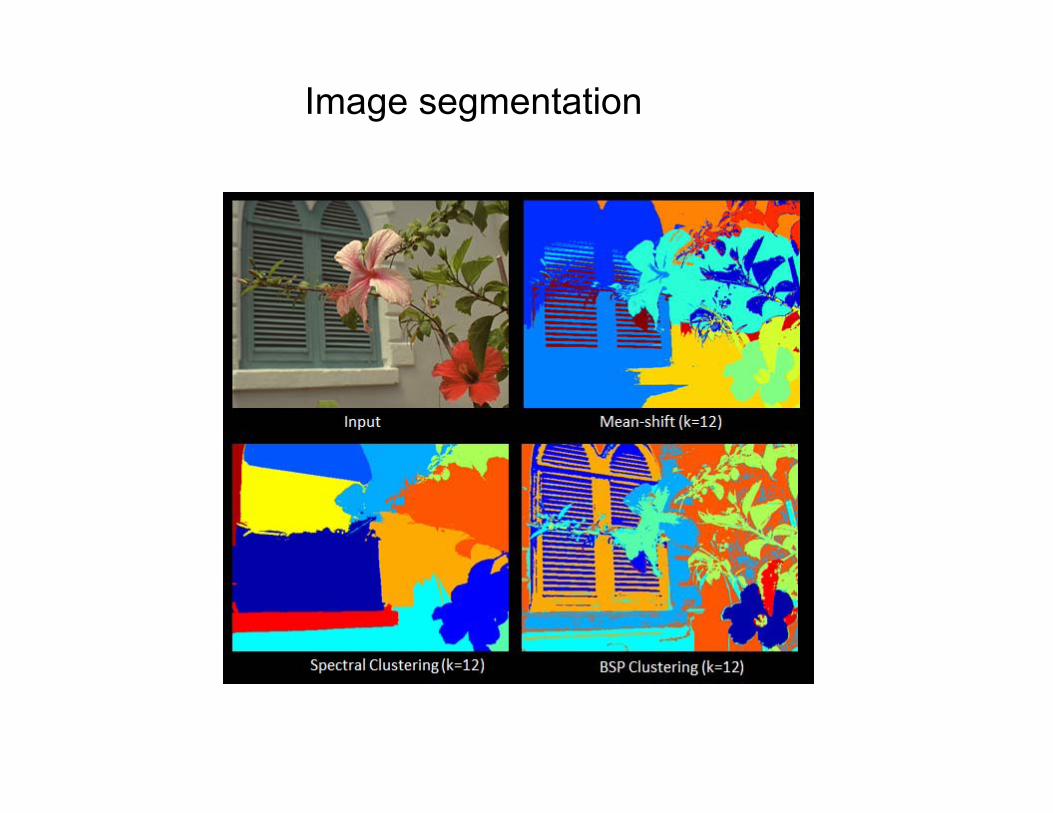
Image segmentation

Image enhancement

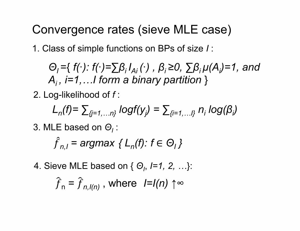
Convergence rates (sieve MLE case)1. Class of simple functions on BPs of size I :

ΘI = f(·): f(·)=∑βi IAi (·) , βi ≥0, ∑βi μ(Ai)=1, and Ai , i=1,…I form a binary partition

2. Log-likelihood of f :

Ln(f)= ∑j=1,…n logf(yj) = ∑i=1,…I ni log(βi)3. MLE based on ΘI :

4. Sieve MLE based on ΘI, I=1, 2, …:

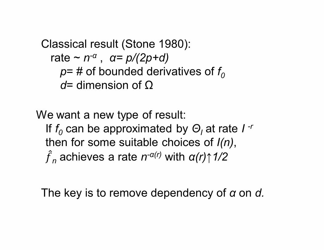
Classical result (Stone 1980): rate ~ n-α , α= p/(2p+d)

p= # of bounded derivatives of f0d= dimension of Ω

The key is to remove dependency of α on d.

δI be the approximation rate of ΘI to f0,

Let HI be the bracketing Hellinger entropy of ΘI, and

Then (with ρ denoting the Hellinger distance),

A relevant result was given in Wong & Shen (1995):

However δI was required to be much stronger than ρ

Result (Linxi Liu & WW)

With r>1/2 and I(n) chosen to be

our sieve MLE has a rate upper bounded by

This result can be used to establish spatial adaptation and variable selection

Acknowledgments

OPT: Li MaBSP: Luo Lu

Clustering & image: TY Wu, CY Tseng

Flow-cytometry: Michael Yang

Compression: Luo Lu, John Mu

---------------------------------------------------------------------------------------

Convergence rate: Linxi Liu