Bandwidth Selection for Multivariate Kernel Density ...repec.org/esAUSM04/up.1603.1077410300.pdf ·...

Bandwidth Selection for Multivariate Kernel Density

Estimation Using MCMC

Xibin Zhang Maxwell L. King Rob J. Hyndman

Department of Econometrics and Business Statistics

Monash University, Clayton, Victoria, 3800, Australia

Correspondence to: [email protected]

July 2004

Abstract: Kernel density estimation for multivariate data is an important technique that has

a wide range of applications in econometrics and finance. However, it has received signifi-

cantly less attention than its univariate counterpart. The lower level of interest in multivariate

kernel density estimation is mainly due to the increased difficulty in deriving an optimal data-

driven bandwidth as the dimension of data increases. We provide Markov chain Monte Carlo

(MCMC) algorithms for estimating optimal bandwidth matrices for multivariate kernel den-

sity estimation. Our approach is based on treating the elements of the bandwidth matrix as

parameters whose posterior density can be obtained through the likelihood cross-validation

criterion. Numerical studies for bivariate data show that the MCMC algorithm generally per-

forms better than the plug-in algorithm under the Kullback-Leibler information criterion, and

is as good as the plug-in algorithm under the mean integrated squared errors (MISE) crite-

rion. Numerical studies for five dimensional data show that our algorithm is superior to the

normal reference rule. Our MCMC algorithm is the first data-driven bandwidth selector for

kernel density estimation with more than two variables, and the sampling algorithm involves

no increased difficulty as the dimension of data increases.

Key Words: Bandwidth matrices; Cross-validation; Kullback-Leibler information; Mean inte-

grated squared errors; Sampling algorithms.

Bandwidth selection for multivariate kernel density estimation using MCMC

1 Introduction

Multivariate kernel density estimation is an important technique in multivariate data analysis

and has a wide range of applications (see, for example, Scott 1992; Aıt-Sahalia 1996; Donald

1997; Stanton 1997; Aıt-Sahalia and Lo 1998). However, its widespread usefulness has been

limited by the difficulty in computing an optimal data-driven bandwidth. We remedy this

deficiency in this paper.

Let X = (X1, X2, . . . , Xd)′ denote a d-dimensional random vector with density f (x) defined on

Rd, and let {x1, x2, . . . , xn} be an independent random sample drawn from f (x). The general

form of the kernel estimator of f (x) is (Wand and Jones 1993):

fH(x) =1n

n

∑i=1

KH(x− xi),

where KH(x) = |H|−1/2K(H−1/2x), K(·) is a multivariate kernel function, and H is a symmet-

ric positive definite d× d matrix known as the bandwidth matrix.

The bandwidth matrix can be restricted to a class of positive definite diagonal matrices, and

then the corresponding kernel function is known as a product kernel. However, there is much

to be gained by choosing a full bandwidth matrix, where the corresponding kernel smoothing is

equivalent to pre-rotating the data by an optimal amount and then using a diagonal bandwidth

matrix. It has been widely recognized that the performance of a kernel density estimator is

primarily determined by the choice of bandwidth, and only in a minor way by the choice of

kernel function (see, for example, Izenman 1991; Scott 1992; Simonoff 1996).

A large body of literature exists on bandwidth selection for univariate kernel density estima-

tion (see, for example, Marron 1987; Jones, Marron and Sheather 1996 for surveys). However,

the literature on bandwidth selection for multivariate data is very limited. Sain, Baggerly and

Scott (1994) discussed the performance of bootstrap and cross-validation methods for band-

width selection in multivariate density estimation and found that the complexity of finding an

optimal bandwidth grows prohibitively as the dimension of data increases. Wand and Jones

(1994) presented a less variable cross-validation algorithm using the plug-in method, which re-

Zhang, King and Hyndman: 2 July 2004 1


quires auxiliary smoothing parameters. The technology for choosing these auxiliary smoothing

parameters is not well developed. Duong and Hazelton (2003) showed that the full bandwidth

matrix selectors suggested by Wand and Jones (1994) fail to produce plug-in bandwidths for

some data sets. In response to this problem, Duong and Hazelton (2003) presented an alter-

native plug-in algorithm for bandwidth selection for bivariate data. This plug-in method has

the advantage that it always produces a finite bandwidth matrix and requires computation of

fewer pilot bandwidths. However, it cannot be directly extended to the general multivariate

setting.

When data are observed from the multivariate normal density and the diagonal bandwidth

matrix, denoted by H = diagonal(h1, h2, · · · , hd), is employed, the optimal bandwidth that

minimizes MISE can be approximated by (Scott 1992; Bowman and Azzalini 1997)

hi = σi

{4

(d + 2)n

}1/(d+4)

,

for i = 1, 2, . . . , d, where σi is the standard deviation of the ith variate and can be replaced by

its sample estimator in practical implementations. We call this the “normal reference rule”.

This method is often used in practice, in the absence of any other practical bandwidth selection

schemes, despite the fact that most interesting data are non-Gaussian.

In theory, the cross-validation criterion can be employed for estimating the optimal bandwidth

for multivariate data. However, it usually involves a numerical optimization, which becomes

increasingly difficult as the dimension of data increases. The MCMC approach avoids this

problem.

To our knowledge, the only previous paper employing an MCMC approach to bandwidth se-

lection for kernel density estimation is Brewer (2000). He derived adaptive bandwidths for

univariate kernel density estimation, treating the bandwidths as parameters and estimating

them via MCMC simulations. Brewer (2000) showed that the proposed Bayesian approach is

superior to methods of Abramson (1982) and Sain and Scott (1996).

Schuster and Gregory (1981) demonstrated that in some circumstances, the likelihood cross-

validation produces inconsistent estimates for univariate kernel density estimation. However,



Brewer (2000) argued that the MCMC approach to adaptive bandwidth selection may avoid

the inconsistency problem by choosing an appropriate prior and using a kernel with infinite

support. The same argument applies to the case considered here.

To estimate the optimal bandwidth matrix for multivariate data, we treat the bandwidth matrix

H as a parameter matrix. The posterior density of H can be obtained through the likelihood

function derived via the likelihood cross-validation criterion. MCMC algorithms can be de-

veloped to sample H from its posterior, and the ergodic average or the posterior mean acts

as an estimator of the optimal bandwidth matrix. One important advantage of the MCMC

approach to bandwidth matrix selection is that it is applicable to data of any dimension, not

only to bivariate data. Moreover, the sampling algorithm involves no increased difficulty as

the dimension of data increases.

In this paper, we present MCMC algorithms for estimating optimal bandwidth matrix for mul-

tivariate kernel density estimation through the likelihood cross-validation criterion, and sam-

pling algorithms are developed for both diagonal and full bandwidth matrices. The rest of

this paper is organized as follows. Section 2 briefly discusses the likelihood cross-validation

criterion and presents MCMC algorithms for both diagonal and full bandwidth matrices. In

Section 3, we examine the performance of MCMC algorithms with data generated from known

bivariate densities. We find that the MCMC algorithm generally performs better than either

the plug-in algorithm or the normal reference rule in the bivariate setting. Section 4 applies

the MCMC bandwidth selectors to data generated from known multivariate densities, and we

find that the MCMC algorithm performs much better than the normal reference rule. Section 5

illustrates the use of the MCMC algorithm for bandwidth selection with an application to some

earthquake data. We provide conclusions in Section 6.



2 MCMC for optimal bandwidth selection

2.1 Likelihood cross-validation

The Kullback-Leibler information is a measure of distance between two densities. Our interest

is in choosing the approximate density fH(x) to minimize its distance from the true density

f (x). In this case, the Kullback-Leibler information is defined as

dKL( f , fH) =∫

log(

f (x)fH(x)

)f (x)dx =

∫log[ f (x)] f (x)dx−

∫log[ fH(x)] f (x)dx , (1)

which is nonnegative. We want to find an optimal bandwidth that minimizes dKL( f , fH), or,

equivalently, maximizes E log[ fH(x)] =∫

log[ fH(x)] f (x)dx, in which the logarithmic pseudo-

likelihood function can be approximated by (see, for example, Hardle 1991)

L(x1, x2, . . . , xn | H) =n

∑i=1

log fH,i(xi), (2)

where fH,i is the leave-one-out estimator

fH,i(xi) =1

n− 1

n

∑j=1j 6=i

|H|−1/2K(

H−1/2(xi − xj))

.

The likelihood cross-validation criterion is to select H by maximizing the average logarithmic

likelihood function n−1L(· | H).

2.2 Sampling a diagonal bandwidth matrix

When H is diagonal, the kernel density estimator of f (x) is

fh(x) =1n

n

∑j=1

1h1h2 · · · hd

K(

x1 − xj,1

h1,

x2 − xj,2

h2, · · · , xd − xj,d

hd

),



where h = (h1, h2, · · · , hd)′ is a vector of bandwidths with positive values. The leave-one-out

estimator is

fh,i(xi) =1

n− 1

n

∑j=1j 6=i

1h1h2 · · · hd

K(

xi,1 − xj,1

h1,

xi,2 − xj,2

h2, · · · , xi,d − xj,d

hd

).

We treat the bandwidth h as a vector of parameters, given which, the likelihood function of

{x1, x2, · · · , xn} is

L(x1, x2, · · · , xn|h) =n

∑i=1

log fh,i(xi).

We assume that the prior density of each component of h is (up to a normalizing constant)

π(hi|λ) ∝1

1 + λ h2i

, (3)

for i = 1, 2, · · · , d, where λ is a hyperparameter controlling the shape of the prior density.

Uniform priors of bandwidths are generally unsuitable, because the update of each hi has a

negligible effect when hi is already very large. However, the prior of hi defined in (3) can pre-

vent the update of hi from getting too large. In a different context, Bauwens and Lubrano (1998)

used a similar prior for the degree-of-freedom parameter of the t-distribution. The purpose of

such priors is to put a low prior probability on the “problematic” region in the parameter space,

where the likelihood function is flat. The joint prior of h, denoted by π(h|λ), is the product of

marginal priors defined in (3). According to Bayes theorem, the logarithmic posterior of h is

(up to an additive constant)

π(h|λ, x1, x2, · · · , xn) ∝ log π(h|λ) +n

∑i=1

log fh,i(xi), (4)

from which we can sample h using the Metropolis-Hastings algorithm. The ergodic average or

the posterior mean of h acts as an estimator of optimal bandwidth.

2.3 Sampling a full bandwidth matrix

As the bandwidth matrix is symmetric positive definite, we can obtain its Cholesky decomposi-

tion H = LL′, where L is a lower triangular matrix. Let B = L−1 which is also lower triangular.



Then the kernel estimator of f (x) is

fB(x) =1n|B|

n

∑i=1

K(

B(x− xi)),

and the leave-one-out estimator of f (x) is

fB,i(xi) =1

n− 1|B|

n

∑j=1j 6=i

K(

B(xi − xj))

.

We treat non-zero elements of the bandwidth matrix as parameters, whose posterior density

can be obtained based on the likelihood function given in (2). We assume that the prior density

of each non-zero component of B is (up to a normalizing constant)

π(bij | λ) ∝1

1 + λ b2ij

(5)

for j ≤ i and i = 1, 2, . . . , d. The joint prior of all elements of B is the product of marginal priors

defined in (5). Using Bayes theorem, we can obtain the logarithmic posterior of B (up to an

additive constant)

π(B | λ, x) ∝d

∑i=1

i

∑j=1

log π(bij | λ) +n

∑i=1

log fB,i(xi), (6)

from which we sample all elements of B using the Metropolis-Hastings algorithm. The ergodic

average or the posterior mean of B acts as an estimator of optimal bandwidth.

2.4 Transformation of data

The plug-in algorithm for bandwidth selection developed by Duong and Hazelton (2003) uses

a simple form for the pilot bandwidths, which is inappropriate when the dispersion of the data

differs markedly between the two variates. Hence Duong and Hazelton (2003) suggested that

the data be pre-scaled before the plug-in algorithm is implemented.

Given a set of bivariate data denoted by {x1, x2, . . . , xn}, let S denote the sample variance-

covariance matrix with diagonal components s21 and s2

2. Duong and Hazelton (2003) defined



the sphering and scaling transformations, respectively, by

x∗i = S−1/2xi, and x∗i = S−1/2d xi,

for i = 1, 2, . . . , n, where Sd = diagonal(s21, s2

2). When the optimal bandwidth matrix, denoted

by H∗, for the transformed data is obtained, the optimal bandwidth matrix for the original data

can be calculated through the reverse transformation, H = S1/2H∗(S1/2)′ or H = S1/2d H∗S1/2

d .

In contrast, the MCMC algorithm does not require such pre-transformations of data. How-

ever, if we choose to make a sphering transformation of data and use the diagonal bandwidth

matrix, the resulting bandwidth estimator for the original data is a full matrix. When the vari-

ates are correlated and the diagonal bandwidth matrix is used, the bandwidth matrix estimator

obtained through the sphering transformation of original data might produce a better perfor-

mance than that obtained directly from the original data, because the sphering transformation

is equivalent to pre-rotating data (see, for example, Wand and Jones 1993).

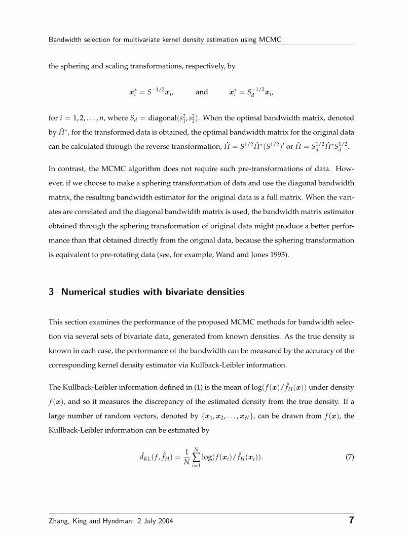
3 Numerical studies with bivariate densities

This section examines the performance of the proposed MCMC methods for bandwidth selec-

tion via several sets of bivariate data, generated from known densities. As the true density is

known in each case, the performance of the bandwidth can be measured by the accuracy of the

corresponding kernel density estimator via Kullback-Leibler information.

The Kullback-Leibler information defined in (1) is the mean of log( f (x)/ fH(x)) under density

f (x), and so it measures the discrepancy of the estimated density from the true density. If a

large number of random vectors, denoted by {x1, x2, . . . , xN}, can be drawn from f (x), the

Kullback-Leibler information can be estimated by

dKL( f , fH) =1N

N

∑i=1

log( f (xi)/ fH(xi)). (7)



3.1 True densities

We consider five target densities labelled A, B, C, D and E. Contour plots of these densities are

shown in Figure 1.

Density A is bivariate normal with high correlation between two variates:

fA(x | µ, Σ) = (2π)−d/2|Σ|−1/2 exp(−1

2(x− µ)′Σ−1(x− µ)

),

with mean µ and variance-covariance matrix Σ given by

µ =

0

0

, Σ =

1 −0.9

−0.9 1

.

Density B is a mixture of two bivariate normal densities, with high correlation and bimodality:

fB(x | µ1, Σ1, µ2, Σ2) =12

fA(x | µ1, Σ1) +12

fA(x | µ2, Σ2),

where

µ1 =

2

2

, Σ1 =

1 −0.9

−0.9 1

, µ2 =

−1.5

−1.5

, Σ2 =

1 0.3

0.3 1

.

Density C is a bivariate skew-normal density with high correlation:

fC(x | µ, Σ, α) = 2φ(x | µ, Σ) Φ(α′W−1/2(x− µ)),

where φ(· | µ, Σ) is the bivariate normal density with mean µ and variance-covariance matrix

Σ, Φ(·) is the cumulative density function of a standard bivariate normal distribution, and W

is a diagonal matrix with diagonal elements the same as those of Σ. This distribution has

recently been studied by Azzalini and Dalla Valle (1996), Azzalini and Capitanio (1999, 2003),

Jones (2001) and Jones and Faddy (2003) among many others. Here α is the shape parameter

capturing the skewness of the distribution. When α = 0, the density fC becomes the usual



normal density. For the purpose of generating a set of data, we use the following parameters,

µ =

2

2

, Σ =

1 0.9

0.9 1

, α =

0.5

0.5

.

Density D is a mixture of two bivariate Student t densities

fD(x | µ1, µ2, Σ, ν) =12

td(x | µ1, Σ, ν) +12

td(x | µ2, Σ, ν),

where

td(x | µ, Σ, ν) =Γ((ν + d)/2)

(νπ)d/2Γ(ν/2)|Σ|1/2

[1 +

1ν(x− µ)′Σ−1(x− µ)

]−(d+ν)/2

, (8)

has location parameter µ, dispersion matrix Σ and degrees of freedom ν, and with parameters

set to

µ1 =

−1.5

0

, µ2 =

1.5

0

, Σ =

1 0.9

0.9 1

,

and ν = 5. Density D exhibits heavy tail behaviour, high correlation and bimodality.

Density E is a mixture of two bivariate Student t densities, but has thicker tails than density D:

fE(x | µ1, µ2, Σ, ν) =12

td(x | µ1, Σ1, ν) +12

td(x | µ2, Σ2, ν),

where ν = 3,

µ1 =

3

3

, Σ1 =

1 0.75

0.75 1

, µ2 =

−3

−3

, and Σ2 =

1 0.5

0.5 1

.

3.2 Bandwidth matrix selectors

From each of the proposed bivariate densities, we generate data sets of size n = 200, 500

and 1000, respectively. For each data set, we calculate the bivariate kernel density estimator

using the bivariate Gaussian kernel function and bandwidth matrix selected through each of



the following selectors.

M1: MCMC algorithm for full bandwidth matrix without pre-transformation of data;

M2: MCMC algorithm for full bandwidth matrix with scaling transformation of data;

M3: MCMC algorithm for full bandwidth matrix with sphering transformation of data;

M4: MCMC algorithm for diagonal bandwidth matrix without pre-transformation of data;

M5: MCMC algorithm for diagonal bandwidth matrix with scaling transformation of data;

M6: MCMC algorithm for diagonal bandwidth matrix with sphering transformation of data;

P1: Plug-in selector of full bandwidth matrix with scaling transformation of data;

P2: Plug-in selector of full bandwidth matrix with sphering transformation of data;

P3: Plug-in selector of diagonal bandwidth matrix with scaling transformation of data;

P4: Plug-in selector of diagonal bandwidth matrix with sphering transformation of data;

A1: The normal reference rule approach for a diagonal bandwidth.

The plug-in bandwidth selector refers to the algorithm developed by Duong and Hazelton

(2003). We have not included the plug-in algorithms of Wand and Jones (1993), because their

algorithm for full bandwidth matrix selection sometimes fails to produce finite bandwidths for

some data sets. When their algorithm works, its performance is similar to the plug-in algorithm

developed by Duong and Hazelton (2003). See Duong and Hazelton (2003) for a discussion on

the advantages of their plug-in algorithm.

3.3 MCMC outputs and sensitivity analysis

The hyperparameter of prior densities defined in (5) is initially set to λ = 1 which represents a

very flat prior. Given a data set generated from a bivariate density, we sample the diagonal and

full bandwidth matrices from their corresponding posterior densities defined in (6) using the

random-walk Metropolis-Hastings algorithm, in which the proposal density is the multivariate

standard normal density, and the tuning parameter is chosen so that the acceptance rate is

between 0.2 and 0.3.

The burn-in period is set at 5,000 iterations, and the number of total recorded iterations is

25,000. The initial value of B is set to the identity matrix. After we obtain the sampled path of



B for each data set, we calculate the ergodic average (or posterior mean) and the batch-mean

standard error (see, for example, Roberts 1996), where the number of batches is 50 and there

are 500 draws in each batch. The ergodic average acts as an estimator of optimal bandwidth.

We use the batch-mean standard error and the simulation inefficiency factor (SIF) to check

the mixing performance of the sampling algorithm (see, for example, Kim, Shephard and Chib

1998; Tse, Zhang and Yu 2004). We use fE(·) as an example to illustrate the mixing performance

of the sampling algorithm. Table 1 presents a summary of MCMC outputs obtained through M1

and M6. Both SIF and the batch-mean standard error show that all the simulated chains have

mixed very well. To demonstrate the mixing performance of these samplers graphically, we

plot the sampled paths, their associated autocorrelation functions and histograms in Figure 2,

which also reveals that these simulated chains have mixed very well. We found similar mixing

performance for the other sampling algorithms, and for the other data sets.

We examined the robustness of the results to prior choices by trying values of λ = 0.1 and

λ = 5, as well as λ = 1. The mixing performance and posterior mean of each sampler was

similar in all cases.

3.4 Accuracy of MCMC bandwidth selectors

In order to estimate the Kullback-Leibler information, we generate N = 100,000 bivariate ran-

dom vectors from the true density and calculate the estimated Kullback-Leibler information

defined by (7), which is employed to measure the distance between the bivariate kernel density

estimator and the corresponding true density. Table 2 presents the estimated Kullback-Leibler

information for each density and each bandwidth selector. The simulation study reveals the

following evidence.

• For data sets generated from fD and fE, the MCMC bandwidth selector performs better

than the corresponding plug-in bandwidth selector; for data sets generated from fB, both

selectors have a similar performance; for data sets generated from fA and fC, the MCMC

bandwidth selector performs better than the plug-in bandwidth selector except when

using a sphering transformation for a full bandwidth matrix.



• For each data set generated, the MCMC bandwidth selector performs better than the

normal reference rule.

• The scaling transformation adds nothing to the performance of MCMC algorithms for

sampling both diagonal and full bandwidth matrices.

• The sphering transformation of data is only helpful to the MCMC algorithm for sampling

a diagonal bandwidth matrix when two variates are correlated, such as for densities A,

C and E. For uncorrelated data, and for sampling a full bandwidth matrix, sphering can

degrade performance. This is also supported by Wand and Jones (1993).

• The MCMC algorithm for a diagonal bandwidth matrix applied after sphering does not

perform quite as well as the full bandwidth approach. However, the simplicity of using

a diagonal bandwidth matrix makes this an attractive approach, especially with high

dimensional data.

We also employ the MISE criterion to examine the performance of optimal bandwidths ob-

tained through the MCMC algorithm, the bivariate plug-in algorithm and the normal reference

rule. We compute numerical MISEs for algorithms M6, P4 and A1 through 50 data sets of sample

sizes 200, 500 and 1000, each of which was generated from fE(·). Results are given in Table 3,

which shows that M6 performs slightly better than P4 for sample size 200, and slightly poorer

than P4 for sample sizes 500 and 1000. We also compute the average difference between inte-

grated squared errors (ISE) of any two bandwidth selectors. The difference of ISEs between M6

and P4 is insignificant, but the difference of ISEs between M6 and A1, as well as that between

P4 and A1, are significant. Both M6 and P4 perform significantly better than A1.

4 Numerical studies with multivariate densities

In this section, we examine the accuracy of the MCMC approach in the general multivariate

setting. Our examples use d = 5.



4.1 True densities and bandwidth selectors

We consider five target densities labelled F, G, H, I and J, respectively.

Density F is a multivariate normal density with location parameter µ and variance-covariance

matrix defined as

Σ =1

1− ρ2

1 ρ ρ2 · · · ρd−1

ρ 1 ρ · · · ρd−2

ρ2 ρ 1 · · · ρd−3

· · · · · ·ρd−1 ρd−2 ρd−3 · · · 1

, (9)

where ρ = 0.9 and µ = (2, 2, 2, 2, 2)′.

Density G is a mixture of two multivariate normal densities,

fG(x | µ1, µ2, Σ) =12

fA(x | µ1, Σ) +12

fA(x | µ2, Σ),

where µ1 = (2, 2, 2, 2, 2)′, µ2 = (−1.5,−1.5,−1.5,−1.5,−1.5)′ and Σ is the identity matrix.

Density H is a mixture of two multivariate Student t densities,

fH(x | µ1, µ2, Σ, ν) =12

td(x | µ1, Σ, ν) +12

td(x | µ2, Σ, ν),

with td(·) defined in (8), µ1 = (2, 2, 2, 2, 2)′, µ2 = (−1.5,−1.5,−1.5,−1.5,−1.5)′, Σ is the identity

matrix, and ν = 3.

Density I is the multivariate skew normal density,

f I(x | µ, Σ, α) = 2φ(x | µ, Σ) Φ(α′W−1/2(x− µ)),

where φ(· | µ, Σ) is the multivariate normal density with location parameter µ and variance-

covariance matrix Σ, Φ(·) is the cumulative density function of a standard multivariate normal

distribution, and W is a diagonal matrix with diagonal elements the same as those of Σ. To gen-

erate a set of data, we define these parameters as µ = (2, 2, 2, 2, 2)′, variance-covariance matrix



Σ defined in (9) with ρ = 0.9, and skewness parameter α = (−0.5,−0.5,−0.5,−0.5,−0.5)′.

Density J is the multivariate skew t density,

f J(x | µ, Σ, ν, α) = 2td(x | µ, Σ, ν)Td(x | ν + d)

where td(·) is the multivariate t density defined in (8), Td(· | ν + d) is the cumulative density

function of a multivariate t distribution with mean 0, identity dispersion matrix and degrees

of freedom ν + d, and

x = α′W−1/2(x− µ)(

ν + d(x− µ)′Σ−1(x− µ) + ν

)1/2

,

with W the diagonal matrix with diagonal elements the same as those of Σ.

From each of the proposed multivariate densities, we generate data sets of sizes 500, 1000 and

1500. Then we apply the proposed MCMC algorithms to each data set to estimate the optimal

bandwidth, where the multivariate standard Gaussian kernel is used. As the normal reference

rule discussed in Scott (1992) and Bowman and Azzalini (1997) is the only viable alternative,

we shall compare the performance of MCMC bandwidth selectors M1 to M6 with that of the

alternative bandwidth selector A1. The MCMC algorithm and parameter settings are the same

as in bivariate examples.

4.2 MCMC outputs and sensitivity analysis

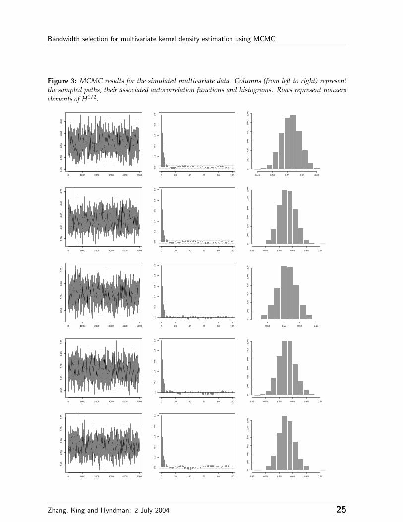
Table 4 shows MCMC output obtained from fF(·) with size 1500 to illustrate the mixing per-

formance of the sampling algorithm. Both the batch-mean standard error and SIF show that all

the sampled chains have mixed very well. Using the output obtained through M1, we plot the

sampled paths, their associated autocorrelation functions and histograms in Figure 3, which

shows that the simulated chains via this algorithm have mixed well.

The numerical study shows that all algorithms for a diagonal bandwidth matrix have a similar

mixing performance, and that all algorithms for a full bandwidth matrix have a similar mixing

performance. However, the algorithm for a diagonal bandwidth matrix usually has a better



mixing performance than that for a full bandwidth matrix. Similar results were found with the

other data sets. Again, we found that MCMC results are insensitive to changes in λ.

4.3 Accuracy of MCMC bandwidth selectors

To estimate the Kullback-Leibler information, we generate N =100,000 random vectors from

the true density and calculate the estimated Kullback-Leibler information defined by (7). Ta-

ble 5 presents these results for each density and each bandwidth selector.

The simulation study reveals the following evidence. First, all MCMC bandwidth selectors

perform much better than the normal reference rule. Second, the scaling transformation adds

nothing to the performance of MCMC algorithms for either the diagonal or full matrices. Third,

the sphering transformation of data is only useful for the diagonal bandwidth matrix when

variables are correlated (such as with densities F, I and J). When there is no correlation, or with

the full bandwidth matrix, sphering degrades performance.

As we did in the bivariate case, we employ the MISE criterion to compare the performance of

optimal bandwidths obtained through the MCMC algorithm and the normal reference rule. We

computed numerical MISEs for algorithms M6 and A1 through 50 data sets of sample size 500,

1000 and 1500, each of which was generated from f I(·). The ISE obtained through M6 is less

than that obtained through A1 for every data set. a summary of numerical ISEs is given in Ta-

ble 6, which shows that the average difference between ISEs of M6 and A1 is highly significant.

5 Application to earthquake data

We now apply the methodology to a trivariate data set discussed in Scott (1992). These data

represent the epicenters of 510 earthquake tremors that occurred beneath the Mt St Helens vol-

cano in the two months leading up to its eruption in March 1982. The three variables represent

latitude, longitude and log-depth below the surface. Scott (1992, plate 8) gives several contours

of a kernel density estimate of these data, where the bandwidths appear to have been chosen

subjectively. We repeat this plot, but using our optimal bandwidth methodology.



We use the MCMC algorithms M1 and M5 to obtain optimal bandwidths, where the hyperpa-

rameter λ = 1, the burn-in period consists of 5,000 iterations, and the recorded period contains

25,000 iterations. Table 7 tabulates a summary of results. Both the batch-mean standard error

and SIF show that all sampled chains have mixed very well.

Using the estimated diagonal bandwidth matrix, we compute a kernel density estimator. (The

estimate using the full bandwidth matrix was almost identical in this case.) The 98% highest

density region (Hyndman 1996) is plotted in Figure 4. The surface was computed using the

algorithm of Amenta, Bern and Kamvysselis (1998). Note that the detached shells represent

outliers in the data; the large central shell represents the bulk of the epicenters. The figure

clearly shows clustering of the epicenters, revealing structure that was not discovered by Scott

(1992) using a subjective bandwidth. It would be interesting to identify the clusters with geo-

logical features, although this information is not available to us.

6 Conclusion

This paper presents MCMC algorithms to estimate the optimal bandwidth for multivariate

kernel density estimation via the likelihood cross-validation criterion. This represents the first

data-driven bandwidth selection method for density estimation with more than two variables.

Our numerical studies show that the sampling algorithms have a very good performance in

achieving convergence of the simulated Markov chains, and are insensitive to prior choices.

Under the Kullback-Leibler information criterion, we have found that the MCMC algorithm

generally performs better than the bivariate plug-in algorithm of Duong and Hazelton (2003)

and the normal reference rule discussed in Scott (1992) and Bowman and Azzalini (1997). Un-

der the MISE criterion, the MCMC algorithm works as well as Duong and Hazelton’s (2003)

plug-in algorithm, and both algorithms are superior to the normal reference rule. Under both

criteria, our sampling algorithm is superior to the normal reference rule for higher dimensional

data. Apart from the superior performance, the other great advantage of our sampling algo-

rithm is that it is applicable to higher dimensional data with no increase in the complexity,

although the computing time required does increase.



Acknowledgements

We extend our sincere thanks to Faming Liang for sharing his coding skills and resources,

David Scott for providing the earthquake data, and Tarn Duong and Martin Hazelton for pro-

viding their R library to compute bivariate plug-in bandwidths. We thank Martin Hazelton

and Gael Martin for helpful comments.

References

Abramson, I. (1982), “On Bandwidth Variation in Kernel Estimates – A Square Root Law,” The

Annals of Statistics, 10, 1217-1223.

Aıt-Sahalia, Y. (1996), “Testing Continuous-Time Models of the Spot Interest Rate,” Review of

Financial Studies, 9, 385-426.

Aıt-Sahalia, Y., and Lo, A.W. (1998), “Nonparametric Estimation of State-Price Densities Im-

plicit in Financial Asset Prices,” The Journal of Finance, 53, 499-547.

Amenta, N., Bern, M., and Kamvysselis, M. (1998) “A New Voronoi-based Surface Reconstruc-

tion Algorithm”, Proceedings of the 25th Annual Conference on Computer Graphics and Interac-

tive Techniques, 415–421.

Azzalini, A., and Capitanio, A. (1999), “Statistical Applications of the Multivariate Skew Nor-

mal Distribution,” Journal of the Royal Statistical Society, Series B, 61, 579-602.

Azzalini, A., and Capitanio, A. (2003), “Distributions Generated by Perturbation of Symmetry

with Emphasis on a Multivariate Skew t-distribution,” Journal of the Royal Statistical Society,

Series B, 66, 367-389.

Azzalini, A., and Dalla Valle, A. (1996), “The Multivariate Skew Normal Distribution,”

Biometrika, 83, 715-726.

Bauwens, L., and Lubrano, M. (1998), “Bayesian Inference on GARCH Models Using the Gibbs

Sampler,” Econometrics Journal, 1, C23-C26.

Bowman, A.W., and Azzalini, A. (1997), Applied Smoothing Techniques for Data Analysis, London:

Oxford University Press.



Brewer, M.J. (2000), “A Bayesian Model for Local Smoothing in Kernel Density Estimation,”

Statistics and Computing, 10, 299-309.

Donald, S.G. (1997), “Inference Concerning the Number of Factors in a Multivariate Nonpara-

metric Relationship,” Econometrica, 65, 103-131.

Duong, T., and Hazelton, M.L. (2003), “Plug-in Bandwidth Selectors for Bivariate Kernel Den-

sity Estimation,” Journal of Nonparametric Statistics, 15, 17-30.

Hardle, W. (1991), Smoothing Techniques with Implementation in S, New York: Springer-Verlag.

Hyndman, R.J. (1996), “Computing and Graphing Highest Density Regions,” American Statisti-

cian, 50, 120-126.

Izenman, A.J. (1991), “Recent Developments in Nonparametric Density Estimation,” Journal of

the American Statistical Association, 86, 205-224.

Jones, M.C. (2001), “A Skew t Distribution,” in Probability and Statistical Models with Applications:

A Volume in Honor of Theophilos Cacoullos,” eds. C.A. Charalambides, M.V. Koutras, and N.

Balakrishnan, London: Chapman & Hall, pp. 269-278.

Jones, M.C., and Faddy, M.J. (2003), “A Skew Extension of the t-distribution, with Applica-

tions,” Journal of the Royal Statistical Society, Series B, 66, 159-174.

Jones, M.C., Marron, J.S., and Sheather, S.J. (1996), “A Brief Survey of Bandwidth Selection for

Density Estimation,” Journal of the American Statistical Association, 91, 401-407.

Kim, S., Shephard, N., and Chib, S. (1998), “Stochastic Volatility: Likelihood Inference and

Comparison with ARCH Models,” Review of Economic Studies, 65, 361-393.

Marron, J.S. (1987), “A Comparison of Cross-Validation Techniques in Density Estimation,”

Annals of Statistics, 15, 152-162.

Roberts, G.O. (1996), “Markov Chain Concepts Related to Sampling Algorithms,” in Markov

Chain Monte Carlo in Practice, eds. W.R. Gilks, S. Richardson, and D.J. Spiegelhalter, London:

Chapman & Hall, pp. 45-57.

Sain, S.R., Baggerly, K.A., and Scott, D.W. (1994), “Cross-Validation of Multivariate Densities,”

Journal of the American Statistical Association, 89, 807-817.

Sain, S.R., and Scott, D.W. (1996), “On Locally Adaptive Density Estimation,” Journal of the

American Statistical Association, 91, 1525-1534.



Schuster, E.F., and Gregory C.G. (1981), “On the Nonconsistency of Maximum Likelihood Non-

parametric Density Estimators,” in Computer Science and Statistics: Proceedings of the 13th

Symposium on the Interface, eds. W.F. Eddy, New York: Springer-Verlag, pp.295-298.

Scott, D.W. (1992), Multivariate Density Estimation: Theory, Practice, and Visualization, New York:

John Wiley.

Simonoff, J.S. (1996), Smoothing Methods in Statistics, New York: Springer-Verlag.

Stanton, R. (1997), “A Nonparametric Model of Term Structure Dynamics and the Market Price

of Interest Rate Risk,” The Journal of Finance, 52, 1973-2002.

Tse, Y.K., Zhang, X., and Yu, J. (2004), “Estimation of Hyperbolic Diffusion with Markov Chain

Monte Carlo Simulation,” Quantitative Finance, 4, 158-169.

Wand, M.P., and Jones, M.C. (1993), “Comparison of Smoothing Parameterizations in Bivariate

Kernel Density Estimation,” Journal of the American Statistical Association, 88, 520-528.

Wand, M.P., and Jones, M.C. (1994), “Multivariate Plug-in Bandwidth Selection,” Computational

Statistics, 9, 97-116.

Wand, M.P., and Jones, M.C. (1995), Kernel Smoothing, London: Chapman & Hall.



Table 1: MCMC results for data generated from fE(·). The first panel is obtained through the algorithmfor a diagonal bandwidth matrix (M6), while the second panel is obtained through the algorithm for afull bandwidth matrix (M1).

sample bandwidths mean standard batch-mean SIF acceptancesize deviation standard error rate200 1/b11 0.70 0.08 0.0017 10.32 0.224

1/b22 0.75 0.07 0.0015 11.77500 1/b11 0.68 0.05 0.0011 11.72 0.207

1/b22 0.66 0.05 0.0009 8.731000 1/b11 0.69 0.03 0.0006 9.83 0.216

1/b22 0.61 0.03 0.0007 11.65200 b11 1.18 0.15 0.0035 14.48 0.245

b21 −1.38 0.34 0.0164 57.58b22 1.69 0.21 0.0098 51.78

500 b11 1.10 0.08 0.0016 11.41 0.265b21 −1.58 0.27 0.0137 65.54b22 1.91 0.19 0.1920 52.87

1000 b11 1.27 0.07 0.0015 11.68 0.267b21 −0.79 0.11 0.0028 16.02b22 1.61 0.08 0.0016 9.45

Table 2: Estimated Kullback-Leibler information for bivariate densities.

sample Kullback-Leibler informationsize M1 M2 M3 M4 M5 M6 P1 P2 P3 P4 A1200 0.046 0.046 0.066 0.101 0.101 0.045 0.117 0.044 0.120 0.203 0.205

E(ln fA) = 500 0.025 0.024 0.041 0.051 0.051 0.026 0.054 0.030 0.057 0.132 0.134−2.003 1000 0.017 0.017 0.018 0.038 0.038 0.020 0.043 0.019 0.047 0.094 0.096

200 0.131 0.129 0.158 0.154 0.154 0.228 0.129 0.213 0.153 0.192 0.375E(ln fB) = 500 0.074 0.075 0.091 0.094 0.094 0.150 0.075 0.124 0.093 0.112 0.284−3.099 1000 0.042 0.042 0.054 0.058 0.058 0.095 0.040 0.067 0.056 0.067 0.235

200 0.032 0.032 0.053 0.089 0.089 0.037 0.100 0.050 0.119 0.105 0.114E(ln fC) = 500 0.021 0.021 0.037 0.048 0.047 0.022 0.047 0.023 0.055 0.089 0.085−1.822 1000 0.018 0.018 0.040 0.040 0.040 0.021 0.038 0.021 0.043 0.065 0.071

200 0.299 0.296 0.247 0.394 0.392 0.361 0.357 0.345 0.391 0.325 0.410E(ln fD) = 500 0.121 0.121 0.129 0.226 0.226 0.220 0.223 0.197 0.263 0.230 0.327−3.072 1000 0.084 0.084 0.101 0.161 0.161 0.140 0.144 0.135 0.187 0.163 0.255

200 0.256 0.254 0.281 0.260 0.260 0.258 0.487 0.417 0.488 0.268 0.461E(ln fE) = 500 0.219 0.221 0.249 0.240 0.240 0.217 0.333 0.298 0.345 0.240 0.385−3.850 1000 0.149 0.149 0.150 0.178 0.178 0.149 0.260 0.222 0.274 0.173 0.299



Table 3: Numerical MISEs for the bivariate density fE(·). “PI” refers to the plug-in method, and“NRR” the normal reference rule. Values in parentheses are the corresponding standard deviations.

sample MISE difference between ISEssize MCMC PI NRR MCMC & PI MCMC & NRR PI & NRR200 0.0077 0.0092 0.0176 -0.00152 -0.00998 -0.00847

(0.00177) (0.00151) (0.00085)500 0.0065 0.0060 0.0149 0.00047 -0.00842 -0.00889

(0.00155) (0.00147) (0.00058)1000 0.0049 0.0041 0.0128 0.00081 -0.00789 -0.00870

(0.00107) (0.00099) (0.00032)

Table 4: MCMC results for data generated from fF(·). The sample size is 1500.

bandwidths mean standard batch-mean SIF acceptancedeviation standard error rate

diagonal 1/b11 0.56 0.03 0.0009 21.85 0.250matrix 1/b22 0.58 0.03 0.0009 24.34

1/b33 0.56 0.03 0.0009 29.251/b44 0.58 0.03 0.0010 36.421/b55 0.58 0.03 0.0009 34.14

full b11 1.81 0.10 0.0042 41.83 0.272matrix b21 −0.15 0.15 0.0106 130.54

b22 1.73 0.09 0.0033 36.26b31 0.11 0.18 0.0143 155.34b32 −0.15 0.13 0.0076 85.27b33 1.80 0.10 0.0031 25.31b41 −0.12 0.14 0.0084 93.56b42 −0.09 0.14 0.0099 133.07b43 −0.02 0.14 0.0083 93.30b44 1.74 0.10 0.0041 46.56b51 0.00 0.14 0.0084 88.95b52 0.07 0.14 0.0098 120.43b53 0.05 0.16 0.0114 134.69b54 0.18 0.13 0.0087 103.13b55 1.78 0.10 0.0042 47.31



Table 5: Estimated Kullback-Leibler information for multivariate densities.

sample Kullback-Leibler informationsize M1 M2 M3 M4 M5 M6 A1500 0.178 0.177 0.539 0.441 0.441 0.186 1.262

E(ln fF) = 1000 0.127 0.126 0.505 0.304 0.304 0.162 1.235−7.9283 1500 0.118 0.117 0.470 0.276 0.276 0.141 1.545

500 0.224 0.224 0.548 0.223 0.223 0.381 1.772E(ln fG) = 1000 0.148 0.148 0.438 0.144 0.144 0.303 1.604−7.7934 1500 0.152 0.151 0.402 0.149 0.149 0.291 1.571

500 0.774 0.771 1.147 0.746 0.746 0.915 2.222E(ln fH) = 1000 0.687 0.685 1.149 0.677 0.677 0.846 1.862−9.2232 1500 0.696 0.696 1.029 0.679 0.680 0.845 1.992

500 0.182 0.180 0.668 0.335 0.334 0.206 1.319E(ln f I) = 1000 0.141 0.140 0.466 0.272 0.272 0.153 1.112−7.5123 1500 0.127 0.126 0.423 0.242 0.242 0.148 1.100

500 0.288 0.282 0.725 0.479 0.479 0.247 1.342E(ln f J) = 1000 0.142 0.141 0.662 0.331 0.331 0.166 1.204−7.3760 1500 0.109 0.109 0.537 0.270 0.270 0.147 1.318

Table 6: Numerical MISEs for the 5-dimension density fE(·).

sample MISE difference between ISEssize MCMC NRR MCMC & NRR standard deviation

500 0.000195 0.000499 -0.000304 0.0000231000 0.000144 0.000421 -0.000278 0.0000151500 0.000125 0.000391 -0.000265 0.000008

Table 7: MCMC results obtained from the Earthquake data.

bandwidths mean standard batch-mean SIF acceptancedeviation standard error rate

diagonal 1/b11 0.003 0.0001 0.000003 9.07 0.254matrix 1/b22 0.003 0.0001 0.000003 12.60

1/b33 0.715 0.0383 0.000873 12.96full b11 311.65 0.07 0.002 15.80 0.246matrix b21 101.53 0.10 0.005 62.21

b22 388.57 0.10 0.003 15.84b31 147.45 0.13 0.008 89.38b32 97.21 0.16 0.011 118.86b33 1.65 0.27 0.012 47.54



Figure 1: Contour graphs of the proposed bivariate densities.Density A

−2 −1 0 1 2

−2

−1

01

2

Density B

−2 0 2 4

−4

−2

02

4

Density C

1 2 3 4

12

34

Density D

−3 −2 −1 0 1 2 3

−3

−2

−1

01

2

Density E

−4 −2 0 2 4

−4

−2

02

4



Figure 2: MCMC results for the simulated bivariate data. Columns (from left to right) show the sampledpaths, their associated autocorrelation functions and histograms. The first two rows represent nonzeroelements of H1/2, while the rest three rows represent elements of B.

0 1000 2000 3000 4000 5000

0.60

0.65

0.70

0.75

0.80

0 20 40 60 80 100

0.0

0.2

0.4

0.6

0.8

1.0

0.60 0.65 0.70 0.75 0.80 0.85

020

040

060

080

010

0012

000 1000 2000 3000 4000 5000

0.55

0.60

0.65

0.70

0.75

0 20 40 60 80 100

0.0

0.2

0.4

0.6

0.8

1.0

0.50 0.55 0.60 0.65 0.70 0.750

200

400

600

800

1000

1200

0 1000 2000 3000 4000 5000

1.0

1.1

1.2

1.3

1.4

1.5

1.6

0 20 40 60 80 100

0.0

0.2

0.4

0.6

0.8

1.0

1.0 1.1 1.2 1.3 1.4 1.5 1.6

020

040

060

080

010

0012

00

0 1000 2000 3000 4000 5000

-1.2

-1.0

-0.8

-0.6

-0.4

0 20 40 60 80 100

0.0

0.2

0.4

0.6

0.8

1.0

-1.2 -1.0 -0.8 -0.6 -0.4

020

040

060

080

0

0 1000 2000 3000 4000 5000

1.4

1.5

1.6

1.7

1.8

1.9

0 20 40 60 80 100

0.0

0.2

0.4

0.6

0.8

1.0

1.4 1.5 1.6 1.7 1.8 1.9 2.0

020

040

060

080

010

0012

00



Figure 3: MCMC results for the simulated multivariate data. Columns (from left to right) representthe sampled paths, their associated autocorrelation functions and histograms. Rows represent nonzeroelements of H1/2.

0 1000 2000 3000 4000 5000

0.45

0.50

0.55

0.60

0.65

0 20 40 60 80 100

0.0

0.2

0.4

0.6

0.8

1.0

0.45 0.50 0.55 0.60 0.65

020

040

060

080

010

0012

000 1000 2000 3000 4000 5000

0.50

0.55

0.60

0.65

0.70

0 20 40 60 80 100

0.0

0.2

0.4

0.6

0.8

1.0

0.45 0.50 0.55 0.60 0.65 0.700

200

400

600

800

1000

1200

0 1000 2000 3000 4000 5000

0.50

0.55

0.60

0.65

0 20 40 60 80 100

0.0

0.2

0.4

0.6

0.8

1.0

0.50 0.55 0.60 0.65

020

040

060

080

010

0012

00

0 1000 2000 3000 4000 5000

0.50

0.55

0.60

0.65

0.70

0 20 40 60 80 100

0.0

0.2

0.4

0.6

0.8

1.0

0.45 0.50 0.55 0.60 0.65 0.70

020

040

060

080

010

0012

00

0 1000 2000 3000 4000 5000

0.50

0.55

0.60

0.65

0.70

0 20 40 60 80 100

0.0

0.2

0.4

0.6

0.8

1.0

0.45 0.50 0.55 0.60 0.65 0.70

020

040

060

080

010

0012

00



Figure 4: The 98% highest density region for the earthquake data showing four views looking fromnorth, east, south and west. Negative log-depth is on the vertical axis, and various combinations oflatitude and longitude are on the horizontal axes.

N E

S W


Date post:	28-Jan-2019
Category:	Documents
Upload:	nguyenhanh
View:	226 times
Download:	0 times

Bandwidth Selection for Multivariate Kernel Density ...repec.org/esAUSM04/up.1603.1077410300.pdf ·...

Documents