Multivariate Signal Processing for Quantitative and...

Multivariate Signal Processing for Quantitative and Qualitative Analysis of Ion Mobility

Spectrometry data, applied to Biomedical Applications and Food Related Applications

Ana Verónica Guamán Novillo

Aquesta tesi doctoral està subjecta a la llicència Reconeixement- CompartIgual 3.0. Espanya de Creative Commons. Esta tesis doctoral está sujeta a la licencia Reconocimiento - CompartirIgual 3.0. España de Creative Commons. This doctoral thesis is licensed under the Creative Commons Attribution-ShareAlike 3.0. Spain License.

FACULTAT DE FÍSICA

Departament d’Electrònica

MEMÒRIA PER OPTAR AL TÍTOL DE DOCTOR PER LA UNIVERSITAT DE

BARCELONA

Doctorat en Enginyeria i Tecnologies Avançades (RD 99/2011)

Multivariate Signal Processing for Quantitative and

Qualitative Analysis of Ion Mobility Spectrometry

data, applied to Biomedical Applications and Food

Related Applications

by

Ana Verónica Guamán Novillo

Director:

Dr. Antonio Pardo

Codirector:

Dr. Josep Samitier

Tutor:

Dr. Antonio Pardo

79

CHAPTER THREE

Experimental Setup and Signal

Processing Strategies.

3.1. Introduction

A discussion about the current status of data analysis of IMS was done in chapter

one, and it was found that univariate strategies are deeply used for IMS data analysis.

However, new applications introduce higher complexity in IMS data and the necessity

to extend the analysis to multivariate strategies. Moreover, IMS can have non-linear

behavior due to both changes of concentration of the analyte of interest and presence

of other substances that impose additional limitations on the use of univariate

techniques.

Since the aim of this thesis is to explore new data analysis strategies for tackling

complex data in bio related applications measured with IMS, a set of dataset were

created for this purposes. The results of this thesis are split in two main parts,

qualitative analysis and quantitative analysis. For the quantitative analysis two set of

synthetic data were generated one of them using pure compounds for testing non-

linear behavior at higher concentrations, and the second one was a mixture of two

amines for evaluating the quantitative effect of them, additional details will be given

below. Moreover, feasible studies were performed for testing IMS as potential device

for on-line measurements. These studies were focused in quality control in wine and

clinical essay. For the qualitative analysis, two non-target dataset were obtained by

analyzing real samples. The goal of the first dataset were to build a discriminative

model for discriminate wine samples of different denomination of origin. The second

one was a preliminary clinical study to classify between rats with sepsis from control

rats through the measurement of volatiles in the rats’ breath. In addition, pre-

processing strategies were evaluated for each spectrometer in order to enhance

signal to noise ratio.

In summary, this chapter explains the experimental setup, specific instrumentation

and the strategies for the data analysis of the studies that were carried out during this

thesis. The first part explains the ion mobility spectrometers used in this thesis with

their main advantages or disadvantages from experimental and data analysis point of

view. Then, each scenario is explained in detail together with the methods and signal

processing strategies. Moreover, block diagram is presented in order to make clear

the signal processing used in each scenario.

Commercial IMS used in the present thesis

80

3.2. Commercial IMS used in the present thesis.

Three different commercial IMS instruments have been used in the present thesis.

Their main features are summarized in Table 3.1 and Table 3.1. As it has been said

in chapter one, the performance of the instruments in presence of some analytes

depends on several key characteristics such as ionization source, sampling

introduction, drift tube temperature, dopant, etc. These three commercial

spectrometers were used taking into account theirs main key characteristics linked to

specific application. Thus, the spectrometer was selected to get the best performance

of the data.

IMS GDA2 G. A. S.

UV-IMS VG-Test

Type Handheld Portable Desktop

Ion source 63Ni

100 MBq

UV Lamp

10.6 eV Corona Discharge

Standard inlet Gas or vapors Gas or vapors Swab

Drift Tube

temperature (ºC) 40-45 Ambient 90

Dopant Water chemistry -None Triethylphosphate

Standard flow of

sample (mL min-1) 400 50-100 240 + pump suction

Drift Gas flow

(mL min-1) 2100 150 200

Shutter Grid Type Bradbury -

Nielson

Bradbury -

Nielson Tyndall-Powell

Opening Time

(sec) 200 500 200

Drift Length (cm) 6.29 12 6.4

Pressure (P) Ambient Ambient Ambient

Inlet Type Membrane Open System Open System

Electric field

(V cm-1) 289 320 280

Peak resolution

Eq. 1.8.(Spangler,

2002)

32 17 18

Sampling rate

(kHz) 33 30 10

Table 3.1 Comparison of the main operation parameters of the three IMS devices used in the present study.

The operation of IMS was explained in chapter one, thereby a summary of its

operation is following explained. The gas phase molecules are sampling into an

ionization source, then an electrostatic gate allows the ions to travel at atmospheric

pressure into the drift tube where a constant electric field accelerates them

(approximately length 6cm). At the end of the drift tube ions become neutralized in the

collector and an electric current is measured. In this manner, the time that the ions

Experimental Setup and Signal Processing Strategies

81

need to reach the collector is measured, depending on the spectrometer the sampling

frequency differs one to each other.

The relevant differences between three spectrometers are ionization source, humidity

membrane, drift tube temperature, and the fact of having or not a dopant. All of these

factors might affect the qualitative and quantitative performance of the spectrometers.

Despite of the fact that in the last four decades a huge variety of both commercial and

handmade IMS has been developed using different ionization sources, drift tube

designs, operating temperatures and ranging in size from pocket size to walk-in

portals, only few direct comparisons of the performance of different instruments are

available. Among of them, comparisons related to the effect of the ionization

source(Borsdorf et al., 2005).

The handheld GDA2 (Airsense, 2012), see Figure 3.1(a), use a radioactive source

which is based on a 100MBeq Ni63 isotope, that works in both positive and negative

mode. That means this spectrometer provide two spectra of the same sample one

related to positive ions and the other to the electronegative ions. The GDA2 also has

a membrane to filter the humidity of the sample and prevent a bad performance of the

IMS. The drift tube has a temperature control to assure a constant temperature and

therefore controlled operation conditions. Moreover, the ionization of this

spectrometer is known as “water chemistry”. Hence, a wider branch of compounds

can be measured above water proton affinity, but not alkanes, which are usually

considered to be biomarkers of some diseases. Other characteristic is the

compounds of this spectrometer has a competitive effect. Therefore, to be able to see

a compound in presence of another one will depend on the proton affinity of them.

The VG-Test (3QBD), see Figure 3.1(b), is a desktop IMS which operation is based

on corona discharge. This IMS is mainly used for biomedical proposes thus a swab is

coupled to the inlet port where the sample is introduced and heated. There is a

temperature control for heating the drift tube and get controlled conditions. The VG-

Test allows adding a dopant for favor compounds with higher proton affinity than the

proton affinity of the dopant. The IMS is set up with a dopant (Triethylphosphate) to

become it selective to amines. A spectrum is taken every 0.63 seconds with a

sampling rate of 10 kHz.

The portable UV-IMS (GAS)), see Figure 3.1 (c), is a portable device which ionization

source is based on UV of 10.6 eV with a constant electric field of 320 V cm–1. The drift

tube works at ambient temperature and the drift gas flow at 100 ml min-1 of Nitrogen.

The sampling rate of the IMS is 30 kHz. A spectrum is average of 32 consecutive

scans. In principle, this spectrometer is able to measure a wide variety of molecules

including alkanes. The fact of not having a temperature control might directly affect to

cluster formation and the identification of compounds. Therefore it is necessary to

have a controlled experiment in order to avoid any bad performance of the

spectrometer.


82

(a)

(b)

(c)

Figure 3.1 Spectrometers used in the current thesis. (a) The handheld GDA2 developed by Airsense, Germany (Airsense, 2012), (b) The portable UV-IMS developed by GAS Dortmund (GAS), (c) the desktop VG-Test developed by 3QBD, Israel (3QBD)

The peak resolution, which in terms of applicability represents the separation between

two peaks, differs between three spectrometers. The peak resolution was defined in

chapter one by Eq. 1.8.(Spangler, 2002). This parameter is calculated using

information from the drift time (td) and the full-width-at-half-height (FWHH) (wh) for the

mobility peak. The peak resolution is a clue parameter for deconvolute overlapping

peaks and in this thesis is used specially in MCR-LASSO algorithm (Pomareda et al.,

2010). In general, high peak resolution implies that overlapped peaks can be

distinguished. In this sense, GDA has higher peak resolution than the other two

spectrometers, therefore GDA in terms of overlapping peaks shows an important

advantage between the other two spectrometers.

It is important to consider that depending on the application, the fact of choosing one

spectrometer or the other will be crucial for obtaining reliable results. In our case,


83

three spectrometers have been used taking into account their main characteristics

related to application. For instance, VG-TEST was used for analyzing biogenic

amines, GDA-2 was used for biomedical and wine applications, and UV-IMS was

used for a non-target study for discrimination of wine. Moreover, additional studies

have been carried out in order to compare IMS performances and main features.

3.2.1. Methods for volatile generation.

In order to achieve the objectives of this thesis, some synthetic experiments are

needed. One of the aims of the synthetic experiments is to find the limit of detection of

some compounds of interest. Therefore, the generation at very low and well

controlled concentrations of different volatiles and mixtures is mandatory. Two

sampling techniques was used to complete this challenge: the use of a volatile

generator equipment and head space sampling.

The volatile generator system (see Figure 3.2) used in this thesis was a commercial

instrument developed by Owlstone (Owlstone, 2014), based on permeation tubes.

The permeation tubes technology allow the generation of precise and repeatable low

concentrations of volatiles. The calibration of the tubes is done through a gravimetric

procedure. The tubes must be weighted and the mass loss is measured over time

using a mass balance. All the procedure lasts several days and the permeation rate is

calculated in ng/min. Once the permeation tubes are calibrated, the tubes can be

used for further analysis, but the generation of low and stable concentrations need an

incubation of the tubes in a very stable temperature and the use of a very controlled

carrier gas flow. The volatile generator instrument helps to have controlled conditions

of temperature and flow.

Figure 3.2 The OVG calibration gas generator developed by Owlstone (Owlstone, 2014) together with IMS used in this present thesis

The head space sampling is normally used for performing synthetic experiments

closer to real scenarios. The sample is heated in order to evaporate the sample for

obtaining the gas phase ions. There are some parameters that need to be set up

such as temperature and the heating time. Many times to control these parameters

are not easy, thus some errors must be expected during the experiment. However,

when the raw sample is liquid or solid, head space sampling is a really good option.

Moreover, depending on the application, other sampling methodologies have to be

used and they are explained depending on the application further on in this chapter.


84

3.2.2. Comparative study of three IMS spectrometers

During this thesis, a comparative study of the performance of three different IMS

spectrometers was done. From this study a publication was realized and published

(Karpas et al., 2013) and for more details refers to this paper.

As far as I know, just few comparative IMS studies had been published before;

among of them the works of Borsdorf et al. should be highlighted (Borsdorf et al.,

2009, Borsdorf et al., 2005, Borsdorf and Rudolph, 2001) in which the gas phase ion-

chemistry of isomeric hydrocarbons (Borsdorf et al., 2005), terpenes (Borsdorf and

Rudolph, 2001) and substituted toluene andaniline compounds (Borsdorf et al., 2009)

was compared when a radioactive 63Ni, a corona discharge (CD) and a

photoionization (PI) ion source was used. One of the most interesting works of

Borsdorf is where he uses three similar RAID1 handheld IMS devices (Bruker,

Germany). The different between the three devices is the ionization source. The work

stands that the reduced mobility and relative abundance of the product ions differed

significantly among these instruments (Borsdorf et al., 2009). A few other reports on

the comparison of the performance of two types of IMS towards detection of odor

signatures of smokeless gun powders (Joshi et al., 2009) and drugs (Su et al., 1998,

Choi et al., 2010) were also published. In many cases vendors of IMS devices report

the level of detection of their device for a given set of compounds (usually belonging

to one of the above applications) allowing consumers to compare the instruments on

the basis of the manufacturers' claims (Cottingham, 2003).

The comparative study done during this thesis, was based on the analysis and

comparison of three important biogenic amines: trimethylamine (TMA), putrescine

(1,4-diaminobutane) and cadaverine (1,5-diminopentane). The sensitivity and limit of

detection for the three amines were determined by continuous monitoring of a stream

of air with a given concentration of the analyte. Ten different concentration with one

replicate were measured and the maximum concentrations (“zero split” in the oven) of

TMA (at 70ºC), putrescine (at 90ºC) and cadaverine (at 90ºC) in a carrier flow either

400 mL min-1 of air were, 11.15, 16.21 and 8.49 ppm (by weight), respectively.

Moreover, measurements of headspace vapors of TMA were also tested in order to

analyze the vapors emanating from a given quantity of the biogenic amine deposited

in a vial. The carrier flow through the headspace vial was 400 mL min-1 for the GDA2

and VG-Test and 100 mL min-1 for the G.A.S. UV instrument. In the VG-Test the

analyte vapors were somewhat further diluted by the instrument's own carrier flow of

240 mL min-1. In addition, the dopant used for each spectrometer in this study is also

different. Toluene was used as a dopant in the UV-IMS instrument, the VG-Test

contained a permeation tube with triethylphosphate (TEP) as a dopant, while the

GDA2 did not contain a dopant and thus the ionization processes are based on so

called "water chemistry". Moreover, the drift tube temperature in the GDA2 was 40-

45ºC, in the VG-Test was 90ºC while the G.A.S. operated at ambient temperature

(about 26ºC).The data analysis of this work is explained in chapter four and five.

The results of this work are relevant in terms of transferability of spectrometers

working at different conditions. The most relevant results will be presented below, for

more detail refers to original paper (Karpas et al., 2013). The results encompass the

raw spectra of each spectrometer, the analysis of the reduced mobilities of each

amine and the calibration sensitivity.


85

The raw spectra of each amine at different concentrations for GDA2, UV-IMS and

VG-Test are shown in Figure 3.3 where the peak of the dopant is pointed out. It can

be notice the differences between the spectra produced by the different the

spectrometers and note how the noise has a different impact on each measurement.

Indeed, while UV-IMS is affected by low frequency environmental interferences which

can be a serious problem at lower concentrations, the other spectrometers are mainly

affected by high frequencies noise. Also, it can be seen the different peaks that can

be obtained using the spectrometers, i.e. GDA2 and VG-Test provide narrower peaks

than UV-IMS. However, the peak resolution of GDA2 is bigger than the others (see

Table 3.1 ), this means the capability of distinguish overlapped peaks. The VG-Test

and UV-IMS has similar peak resolution, but VG-Test use a dopant that favor amines

and rejecting compounds of less proton affinity. That is the reason why the spectra of

UV-IMS shows peaks more overlapped than the others.

Signal processing steps were applied to each spectrum in order to enhance the signal

to noise ratio (SNR) for each spectrometer. The signal to noise ratio (SNR) improved

due to the pre-processing from 8 to 16 dB for the VG-Test, from 7 to 12 dB for the

GAS and from 10 to 42 dB for the GDA2. The methodology used for obtaining these

results is explained in detail in chapter four.

(a)


86

(b)

(c)

Figure 3.3 Raw spectra from three amines (a) GDA2 (Ni-IMS) Airsense (b) UV-IMS (G.A.S Durtmund) and (c) VG-TEST (3QBD, Israel)


87

The reduced mobility values of the ions formed in TMA, putrescine and cadaverine

were determined relative to that of 2,4-lutidine (Eiceman et al., 2003) and are shown

in Table 3.2. The protonated monomer molecule was seen in all spectrometers;

however the reduced mobility values differ significantly in some cases. The reduced

mobility value for the putrescine protonated monomer measured with the GDA2

instrument (1.94 cm2V-1s-1) differed significantly from the value obtained with UV-IMS

(1.99 cm2V-1s-1) and the VG-Test device in the present study (2.02 cm2V-1s-1).

Nonetheless, in studies carried out with the VG-Test at 3QBD measuring putrescine

or cadaverine vapors emanating from a sample that was placed on a cotton swab, an

additional peak for the monomers with reduced mobility values of 1.93 and 1.84 cm2V-

1s-1, respectively, with slightly longer drift times were observed and the relative

intensity of the two species changed during the measurement probably due to

variations in the operational conditions (Karpas et al., 2013) . Note that for a given

analyte in a given instrument, the drift time and reduced mobility did not change with

concentration or with the sample introduction method.

The differences observed in the reduced mobility values cannot be attributable to

uncertainties in drift time measurements and mobility scale calibrations. The

differences might be due to formation of different ion species in each IMS that has

been operating at different conditions (ion source, temperature, moisture, reactant ion

chemistry and structural features of the drift tube). Thus, discrepancies in reduced

mobility values that have been reported for different IMS devices are not necessarily

the result of erroneous measurements but rather a natural outcome of variations in

ionic species formed under different experimental conditions. This may have major

repercussions on the transferability of reduced mobility values between different

instruments and even for the same instrument operated under different conditions.

This also could be attributed to variation in the degree of clustering that is affected by

the different operating temperatures of the three devices and to the nature and

characteristics of the core ion.

Compound

Temperature

Ion Species

Reduced Mobilities

GDA2

44ºC

G. A. S.

26ºC

VG-Test

90ºC

2,4-Lutidine (LUT)H+ 1.90 1.90 1.90

TMA (TMA)H+ 2.22 2.13 2.10

(TMA)2H+ 1.78 - -

Putrescine (PUT)H+ 1.94 1.99 2.02

(PUT)2H+ 1.46 - -

Cadaverine (CAD)H+ 1.81 1.82 1.87

(CAD)2H+ 1.36 - -

Mixed (CAD)(PUT)H+ 1.41 - - Table 3.2 The ion species observed in TMA, putrescine (PUT) and Cadaverine(CAD) and their reduced mobility values (cm2V-1s-1) calculated relative to 2,4-lutidine(LUT)


88

There have been other studies regarding different product ions that can be found in

different IMS operating with identical parameters except the ion source used

(Borsdorf et al., 2009). Quantitative measurements to determine the limit of detection

were not reported in that study (Borsdorf and Rudolph, 2001). From these results can

be concluded that IMS needs to be calibrated before performing any experiment;

however the current database of reduced mobility can serve only as a guideline for

identification of ion species.

Since the main objective of this study is to determine meaningful differences between

different commercial spectrometers working at different conditions, it is necessary to

perform accurate spectra analysis. Therefore, multivariate signal processing was

carried out for extracting significant information and performing a proper analysis of

the final results.

The quantitative response of the IMS was performed using multivariate strategies.

Multivariate strategies, in contrast with univariate methodologies, allow evaluating the

overall spectra and getting information regarding the evolution of the ions species

present in the samples. Although multivariate strategies are deeper explained in

chapter five, a brief summary is presented below.

The IMS spectra needs to be preprocessed in order to enhance the signal to noise

ratio (see chapter four). The determination of the pure components in the sample is

necessary for a good performance of the quantification of IMS measurements.

Multivariate curve resolution (MCR) has been used as a multivariate solution for this

task, specifically MCR-Lasso (Pomareda et al., 2010) was implemented. MCR-Lasso

is a hard source technique, where Gaussian Models are imposed for building the final

model. This means that noise is quite to be modelled by a Gaussian and therefore

only the most relevant peaks are shaped. Then, a calibration model was built for

analyzing the performance of the three spectrometers.

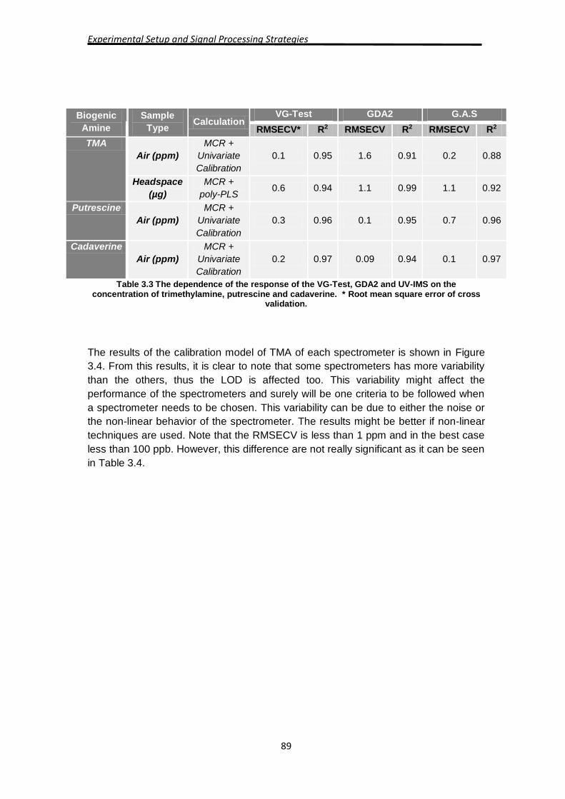
The final performance of the calibration model for cadaverine, putrescine and TMA is

summarized in Table 3.3. It can be seen that the sensitive of the calibration model do

not vary from spectrometer to spectrometer and is closer to one, but the root mean

square error of cross validation (RMSECV) changes from both spectrometer and

biogenic amine. The RMSECV was evaluated leaving samples out during the model

construction. This might be due to either the noise present in the sample or the

sensitivity or selectivity of the spectrometer to the biogenic amine.


89

Biogenic

Amine

Sample

Type Calculation

VG-Test GDA2 G.A.S

RMSECV* R2 RMSECV R2 RMSECV R2

TMA

Air (ppm)

MCR +

Univariate

Calibration

0.1 0.95 1.6 0.91 0.2 0.88

Headspace

(µg)

MCR +

poly-PLS 0.6 0.94 1.1 0.99 1.1 0.92

Putrescine

Air (ppm)

MCR +

Univariate

Calibration

0.3 0.96 0.1 0.95 0.7 0.96

Cadaverine

Air (ppm)

MCR +

Univariate

Calibration

0.2 0.97 0.09 0.94 0.1 0.97

Table 3.3 The dependence of the response of the VG-Test, GDA2 and UV-IMS on the concentration of trimethylamine, putrescine and cadaverine. * Root mean square error of cross

validation.

The results of the calibration model of TMA of each spectrometer is shown in Figure

3.4. From this results, it is clear to note that some spectrometers has more variability

than the others, thus the LOD is affected too. This variability might affect the

performance of the spectrometers and surely will be one criteria to be followed when

a spectrometer needs to be chosen. This variability can be due to either the noise or

the non-linear behavior of the spectrometer. The results might be better if non-linear

techniques are used. Note that the RMSECV is less than 1 ppm and in the best case

less than 100 ppb. However, this difference are not really significant as it can be seen

in Table 3.4.


90

(a)

(b)

(c)

Figure 3.4 Calibration model of TMA for each spectrometer. (a) GDA, (b) UV-IMS and (c) VG-Test.

On the other hand, the response of the three IMS devices to TMA vapors in a

headspace vial was similar in principle though different in detail. This is clear seen in

Figure 3.5 (a) that shows the TMA and reactant ion peak in the VG-Test as function of

time. First, a rapid increase within a few seconds in the intensity of the analyte signal,

concomitant with the decrease in the reactant ion peak and then a gradual decrease

in the analyte signal and increase in the reactant ion peak as the headspace vapors

begin to clear out. These changes are due to the fact that the flow of the carrier

through the headspace vial dilutes the analyte vapors and the rate of dilution depends

on the flow and volume of the vial.

0 1 2 3 4 5 6 7 8-1

0

1

2

3

4

5

6

7

8

Real Concentration (ppm)

Pre

dic

ted

Co

nce

ntr

atio

n (

pp

m)

Univariate Calibration (GDA2) Correction

LOD: 0.8 ppm

RMSECV: 0.7 ppmLOD

0 0.5 1 1.5 2 2.5 3 3.5 4-0.5

0

0.5

1

1.5

2

2.5

3

3.5

4


Pre

dic

ted

Co

nce

ntr

atio

n (

pp

m)

Univariate Calibration (UV-IMS)

LOD

LOD: 0.5 ppmRMSECV: 0.2 ppm

0 1 2 3 4 5 6

0

1

2

3

4

5

6


Co

nce

ntr

atio

n P

red

icte

d (

pp

m)

Univariate Calibration (VG-Test) Correction

LOD

LOD: 0.1 ppmRMSECV:0.06 ppm


91

(a)

(b)

(c)

Figure 3.5 The signal intensity of the analyte (TMA) and reactant ion (TEP) peak in headspace vial as a function of time. (b) The theoretical (with pefect mixing) dilution of the TMA headspace

analyte vapor for a carrier flow of 400 ml min-1 (6.67 ml s-1) and a 20 ml vial volume for VG-Test. (c) Final calibration model using poly-PLS. The predicted concentration vs Real concentration in

which the final model have a 3 latent variables and a polynomial of order 2.

Theoretically, with perfect mixture, a carrier flow of 400 ml min-1 (6.67 ml s-1) with a

20 ml vial volume should dilute the analyte vapors as shown in Figure 3.5 (b). For the

VG-Test the graph was adjusted to allow for the 5 seconds delay until the maximum

signal intensity of the analyte is obtained. Evidently, the clearing time is longer due to

imperfect mixing and transport of analyte vapors from the sample vial into the drift

tube. In Figure 3.5 (c) is shown the final model for TMA headspace vapors measured

in VG-Test after applying MCR and poly-PLS which number of latent variables and

polynomial order were set up by cross validation. The fact of using poly-PLS was due

to the non-linear data that was obtained for analyzing head-space samples. In this

case, the latent variables were selected by 3 and the order of the polynomial was 2.

The final calibration results and limit of detection calculated according it was

explained in methodology part are shown in Table 3.3 and Table 3.4.

2.4 4.8 7.2 9.6 12 14.4

0

2.4

4.8

7.2

9.6

12

14.4

TMA HS Measured (ug)

TM

A H

S P

red

icte

d (

ug

)

Calibation curve (VG-Test)

LOD

0 10 20 30 40 50 600

0.5

1

1.5

2

2.5x 10

5

Time (s)

Peak (

a.u

.)

VG-Test

TMA-Measured

Theoretical


92

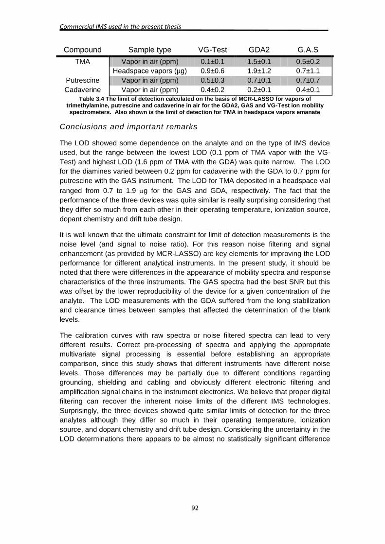
Compound Sample type VG-Test GDA2 G.A.S

TMA Vapor in air (ppm) 0.1±0.1 1.5±0.1 0.5±0.2

Headspace vapors (µg) 0.9±0.6 1.9±1.2 0.7±1.1

Putrescine Vapor in air (ppm) 0.5±0.3 0.7±0.1 0.7±0.7

Cadaverine Vapor in air (ppm) 0.4±0.2 0.2±0.1 0.4±0.1

Table 3.4 The limit of detection calculated on the basis of MCR-LASSO for vapors of trimethylamine, putrescine and cadaverine in air for the GDA2, GAS and VG-Test ion mobility spectrometers. Also shown is the limit of detection for TMA in headspace vapors emanate

Conclusions and important remarks

The LOD showed some dependence on the analyte and on the type of IMS device

used, but the range between the lowest LOD (0.1 ppm of TMA vapor with the VG-

Test) and highest LOD (1.6 ppm of TMA with the GDA) was quite narrow. The LOD

for the diamines varied between 0.2 ppm for cadaverine with the GDA to 0.7 ppm for

putrescine with the GAS instrument. The LOD for TMA deposited in a headspace vial

ranged from 0.7 to 1.9 g for the GAS and GDA, respectively. The fact that the

performance of the three devices was quite similar is really surprising considering that

they differ so much from each other in their operating temperature, ionization source,

dopant chemistry and drift tube design.

It is well known that the ultimate constraint for limit of detection measurements is the

noise level (and signal to noise ratio). For this reason noise filtering and signal

enhancement (as provided by MCR-LASSO) are key elements for improving the LOD

performance for different analytical instruments. In the present study, it should be

noted that there were differences in the appearance of mobility spectra and response

characteristics of the three instruments. The GAS spectra had the best SNR but this

was offset by the lower reproducibility of the device for a given concentration of the

analyte. The LOD measurements with the GDA suffered from the long stabilization

and clearance times between samples that affected the determination of the blank

levels.

The calibration curves with raw spectra or noise filtered spectra can lead to very

different results. Correct pre-processing of spectra and applying the appropriate

multivariate signal processing is essential before establishing an appropriate

comparison, since this study shows that different instruments have different noise

levels. Those differences may be partially due to different conditions regarding

grounding, shielding and cabling and obviously different electronic filtering and

amplification signal chains in the instrument electronics. We believe that proper digital

filtering can recover the inherent noise limits of the different IMS technologies.

Surprisingly, the three devices showed quite similar limits of detection for the three

analytes although they differ so much in their operating temperature, ionization

source, and dopant chemistry and drift tube design. Considering the uncertainty in the

LOD determinations there appears to be almost no statistically significant difference


93

between these three instruments. This finding may have general implications as to

the possible limit of detection that can be achieved with classic IMS drift tubes

(without pre-concentration or separation).

3.3. Data set used in this thesis: Motivation, work scenarios and

signal processing methodologies.

From the last section (Section 3.2) it was seen that studies performed in different

commercial IMS can be comprable and are likely to provide similar results.

Nevertheless, it is clear that IMS needs to be often calibrated before performing any

experiment. Another important issue that was treated in the last section was the need

of using a proper multivariate signal analysis, in order to get the most relevant

information.

The thesis aims to introduce strategies for the analysis of IMS spectra. Furthermore,

the novel bio-related applications that have been faced by the IMS technologies in the

last years have also brought new issues to be solved in terms of IMS signal

processing. The complexity and high dimensionality of data provided by bio-related

scenarios makes mandatory the use of proper signal processing algorithms for

obtaining good performance. In order to study and test different algorithmic signal

processing solutions for IMS data about bio-related datasets, a set of experiments

were developed during this thesis. The detail of these experiments are presented

below.

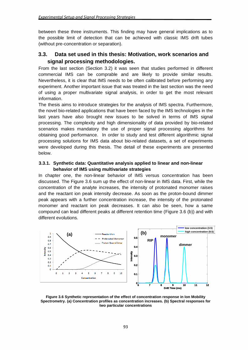
3.3.1. Synthetic data: Quantitative analysis applied to linear and non-linear

behavior of IMS using multivariate strategies

In chapter one, the non-linear behavior of IMS versus concentration has been

discussed. The Figure 3.6 sum up the effect of non-linear in IMS data. First, while the

concentration of the analyte increases, the intensity of protonated monomer raises

and the reactant ion peak intensity decrease. As soon as the proton-bound dimmer

peak appears with a further concentration increase, the intensity of the protonated

monomer and reactant ion peak decreases. It can also be seen, how a same

compound can lead different peaks at different retention time (Figure 3.6 (b)) and with

different evolutions.

Figure 3.6 Synthetic representation of the effect of concentration response in Ion Mobility Spectrometry. (a) Concentration profiles as concentration increases. (b) Spectral responses for

two particular concentrations

6 7 8 9 10 11 120

0.1

0.2

0.3

0.4

0.5

Drift Time (ms)

Inte

ns

ity

low concentration (3.5)

high concentration (9.5)

RIP

monomer

dimmer

(a) (b)

6 7 8 9 10 11 120

0.1

0.2

0.3

0.4

0.5

Drift Time (ms)

Inte

ns

ity

low concentration (3.5)

high concentration (9.5)

RIP

monomer

dimmer

(a) (b)

Dataset used in this thesis: Motivation, work scenarios and signal processing methodologies

94

The quantitative analysis for IMS has received scarce attention such as it was

mentioned in chapter two. The default solution is the use of univariate techniques,

which are usually performed through the information of peak area or peak height of

protonated monomer or protonated-bound dimmer and then applying an appropriate

fitting function, commonly a polynomial function. However, it is known that the

monomer is sensitive at low concentrations and the protonated-bound dimmer usually

appears at high concentrations. Moreover, the IMS dynamics is non-linear when

concentration is increasing, thus the univariate techniques are not fully suitable;

whereas, multivariate calibration techniques appear to be a good choice for dealing

with these conditions.

Regarding multivariate calibration techniques PLS has been studied by different

authors (Zheng et al., 1996, Fraga et al., 2009). The studies show that multivariate

calibration methods provide better IMS quantitative precision and accuracy than

univariate methods even when the peaks are unresolved. Nevertheless, the

interpretation of PLS models for IMS is not easy. Furthermore, despite the fact that

PLS algorithm is able to handle slightly non-linear data by increasing the number of

latent variables in the calibration model, this approach is less successful for datasets

containing moderate and severe non-linearities (Yang et al., 2003). A different

approach to analyze IMS spectra is the use of multivariate curve resolution

techniques (MCR) that aim to recover the evolution of the source signals

(concentration profiles) and the mixing matrix (spectral features) without any prior

supervised calibration step. Therefore, it provides a powerful way to separate

contributions of substances as separated components without having any prior

knowledge about the composition of the sample.

In the present work, we aim to provide a multivariate calibration method for IMS

spectra combining the advantages of MCR-ALS for qualitative interpretation and a

non-linear multivariate technique such as poly-PLS for an improved quantification of

substance concentration. Thereby, MCR-ALS is used as a prior step to multivariate

calibration modeling nonlinear contributions properly and with an easier interpretation.

This method can be useful especially in cases where peak intensity behavior is non-

linear as concentration increases.

Methods and Sample preparation

Standards of 2-butanone and ethanol samples (at least 99% pure, provided by

Sigma-Aldrich) were prepared at different concentrations using synthetic air premier

(pure at 99.995%, provided by Carburos Metálicos). The standards were obtained by

a volatile generator system based on permeation tubes (OVG4, Owlstone). The

permeation tubes were previously calibrated in our facilities by gravimetric methods

after one week in the OVG4 at constant temperature. The analytes were measured

using the GDA2 ion mobility spectrometer (Airsense, 2012) at ten different

concentrations and each set of measurements were repeated in three different days.

Table 3.5 shows the measured concentrations for each substance. Twenty spectra

(consecutive scans) are obtained for each concentration. The same measurements

were replicated in three different days. In the case of 2-butanone, the total size of the

data matrix is 108 scans x 198 spectral points for each replicate. In the case of


95

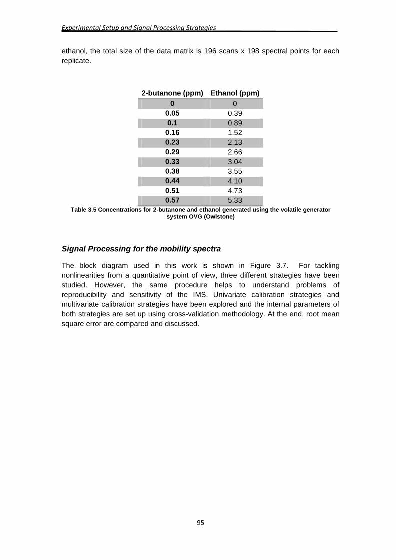
ethanol, the total size of the data matrix is 196 scans x 198 spectral points for each

replicate.

2-butanone (ppm) Ethanol (ppm)

0 0

0.05 0.39

0.1 0.89

0.16 1.52

0.23 2.13

0.29 2.66

0.33 3.04

0.38 3.55

0.44 4.10

0.51 4.73

0.57 5.33

Table 3.5 Concentrations for 2-butanone and ethanol generated using the volatile generator system OVG (Owlstone)

Signal Processing for the mobility spectra

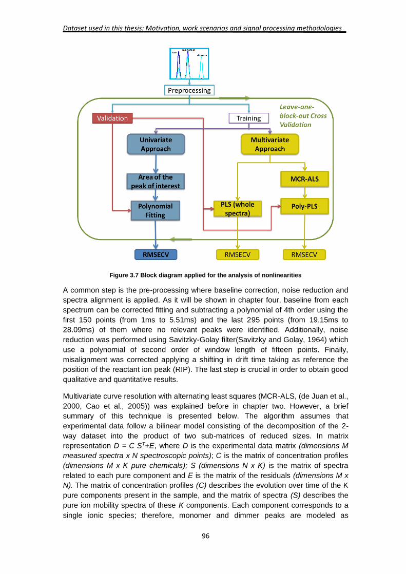
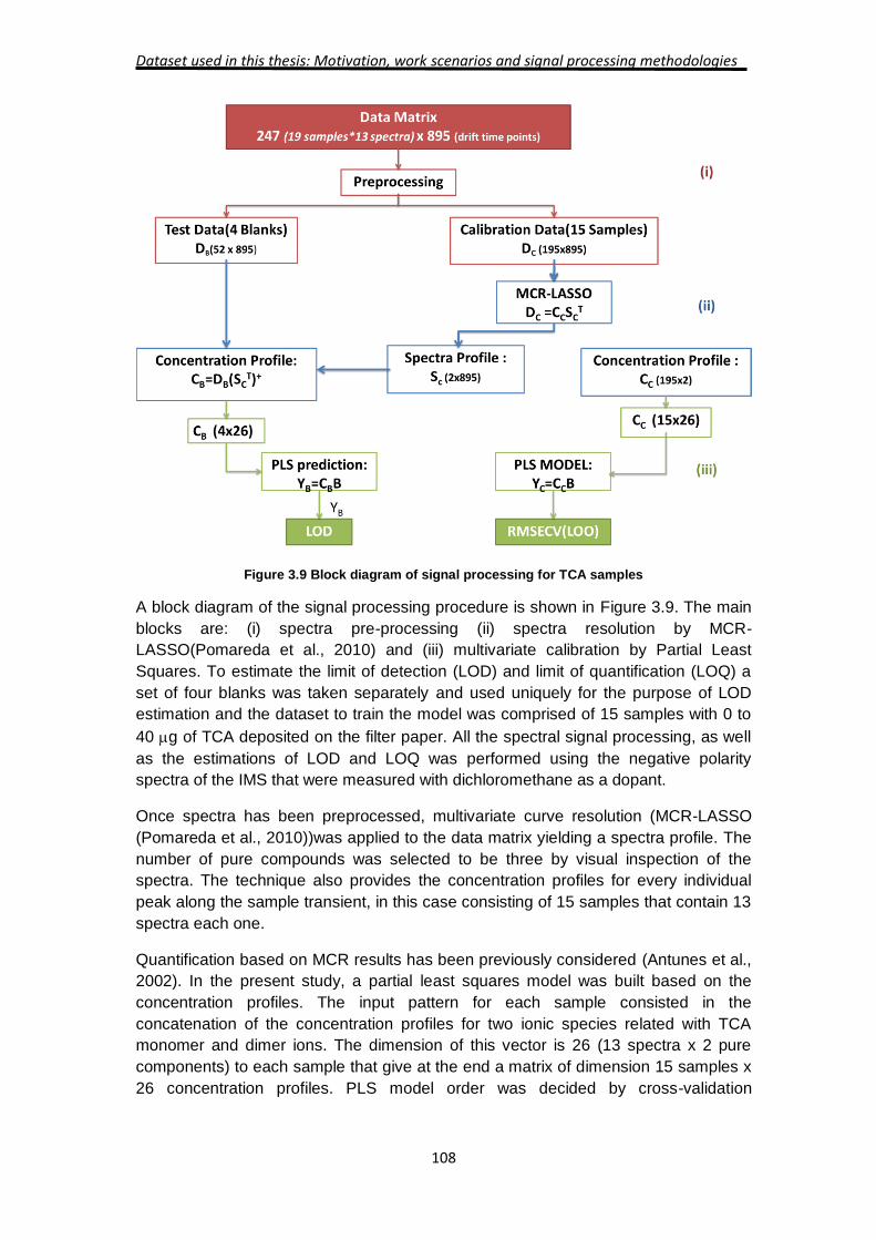
The block diagram used in this work is shown in Figure 3.7. For tackling

nonlinearities from a quantitative point of view, three different strategies have been

studied. However, the same procedure helps to understand problems of

reproducibility and sensitivity of the IMS. Univariate calibration strategies and

multivariate calibration strategies have been explored and the internal parameters of

both strategies are set up using cross-validation methodology. At the end, root mean

square error are compared and discussed.


96

Figure 3.7 Block diagram applied for the analysis of nonlinearities

A common step is the pre-processing where baseline correction, noise reduction and

spectra alignment is applied. As it will be shown in chapter four, baseline from each

spectrum can be corrected fitting and subtracting a polynomial of 4th order using the

first 150 points (from 1ms to 5.51ms) and the last 295 points (from 19.15ms to

28.09ms) of them where no relevant peaks were identified. Additionally, noise

reduction was performed using Savitzky-Golay filter(Savitzky and Golay, 1964) which

use a polynomial of second order of window length of fifteen points. Finally,

misalignment was corrected applying a shifting in drift time taking as reference the

position of the reactant ion peak (RIP). The last step is crucial in order to obtain good

qualitative and quantitative results.

Multivariate curve resolution with alternating least squares (MCR-ALS, (de Juan et al.,

2000, Cao et al., 2005)) was explained before in chapter two. However, a brief

summary of this technique is presented below. The algorithm assumes that

experimental data follow a bilinear model consisting of the decomposition of the 2-

way dataset into the product of two sub-matrices of reduced sizes. In matrix

representation D = C·ST+E, where D is the experimental data matrix (dimensions M

measured spectra x N spectroscopic points); C is the matrix of concentration profiles

(dimensions M x K pure chemicals); S (dimensions N x K) is the matrix of spectra

related to each pure component and E is the matrix of the residuals (dimensions M x

N). The matrix of concentration profiles (C) describes the evolution over time of the K

pure components present in the sample, and the matrix of spectra (S) describes the

pure ion mobility spectra of these K components. Each component corresponds to a

single ionic species; therefore, monomer and dimmer peaks are modeled as


97

separated components. The constraints used in this work were: unimodality, closure

and non-negative. Non-negativity has been used because concentration profiles and

spectra are expected to be positive in order to have a physical and chemical

meaning. This constraint has been applied through fast nonnegative least squares

(FNNLS (Bro and DeJong, 1997)). Moreover unimodality has been applied in peaks

which were expected to be unimodal for instance, the reactant ion peak and the

monomer. The closure constraint has also been applied because, in IMS, available

charge is transferred among ions but this charge remains constant during the whole

process; this constraint is applied to all concentration profiles. In addition, self-

modelling mixture analysis (SIMPLISMA (Windig et al., 2002)) was used to obtain

initial estimations.

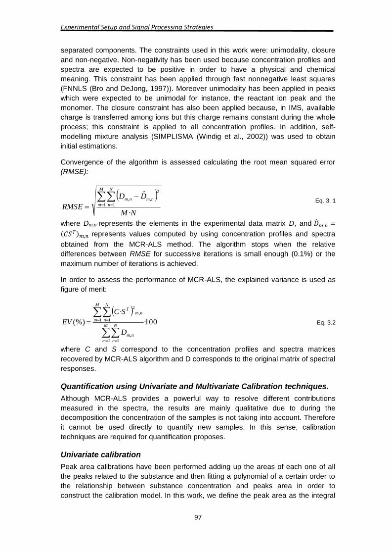
Convergence of the algorithm is assessed calculating the root mean squared error

(RMSE):

NM

DD

RMSE

M

m

N

n

nmnm

·

ˆ

1 1

2

,,

Eq. 3. 1

where Dm,n represents the elements in the experimental data matrix D, and �̂�𝑚,𝑛 =

(𝐶𝑆𝑇)𝑚,𝑛 represents values computed by using concentration profiles and spectra

obtained from the MCR-ALS method. The algorithm stops when the relative

differences between RMSE for successive iterations is small enough (0.1%) or the

maximum number of iterations is achieved.

In order to assess the performance of MCR-ALS, the explained variance is used as

figure of merit:

100·

·

(%)

1 1

,

1 1

,

2

M

m

N

n

nm

M

m

N

n

nmT

D

SC

EV

Eq. 3.2

where C and S correspond to the concentration profiles and spectra matrices

recovered by MCR-ALS algorithm and D corresponds to the original matrix of spectral

responses.

Quantification using Univariate and Multivariate Calibration techniques.

Although MCR-ALS provides a powerful way to resolve different contributions

measured in the spectra, the results are mainly qualitative due to during the

decomposition the concentration of the samples is not taking into account. Therefore

it cannot be used directly to quantify new samples. In this sense, calibration

techniques are required for quantification proposes.

Univariate calibration

Peak area calibrations have been performed adding up the areas of each one of all

the peaks related to the substance and then fitting a polynomial of a certain order to

the relationship between substance concentration and peaks area in order to

construct the calibration model. In this work, we define the peak area as the integral


98

of the peak corresponding to the FWHM (Full Width Half Maximum) region, that is,

the sum of intensities above the 50% of the maximum. The polynomial order is

optimized using a cross-validation procedure and peak height calibrations have been

performed in a similar way to area calibration but taking the maximum of the

monomer peak.

Partial least squares (PLS) and nonlinear polynomial PLS (poly-PLS)

PLS and poly-PLS have been applied to both the original matrices of spectral

responses which are considered to be the X-block and the concentration profile from

MCR-ALS. In these cases, the number of latent variables (PLS and poly-PLS) and the

polynomial order (poly-PLS) were optimized using a cross validation procedure in

order to construct the calibration model.

The main proposal in this work is to build multicalibration models using the

concentration profiles extracted by a pre-processing MCR-ALS step. For that

purpose, PLS and poly-PLS have also been applied to the matrices constructed using

the concentration profiles of monomer and dimmer (obtained from MCR-ALS). In

these cases, the number of latent variables was set to be 2 (monomer and dimmer)

and only the polynomial order (poly-PLS) was needed to be optimized using the cross

validation procedure.

Cross validation: Leave-One-Block-Out

Cross-validation can be used to achieve two main objectives: assessing the

performance of the different calibration techniques (univariate and multivariate cases)

and optimizing some parameters (the number of latent variables in PLS and poly-PLS

and the polynomial order in the univariate techniques and the poly-PLS case).

The cross-validation procedure used in the present work corresponds to leave-one-

block-out (LOBO). First of all, the set of spectra corresponding to the first and last

measured concentrations are always used to construct the calibration model, which

means that this set of samples is not available for validation. The reason is that we

are interested in predicting concentrations within a certain range and not out of this

range. This requirement could not be fulfilled if the first or last concentration were

taken out to be validated. Secondly, leaving one block out means that, given a

substance, the set of spectra corresponding to a certain test concentration is taken

out to be validated and the remaining set of samples is used to build the calibration

model. In other words, the estimation dataset never has the concentration value that

is going to be predicted. In this way, the interpolation performance of the model is

tested. The set of scans to be validated for each concentration is used to calculate

the root mean squared error of validation (RMSEV).

V

cc

RMSEV

V

v

PREDICTEDREAL

1

2)ˆ(

Eq. 3.3

where REALc corresponds to the original concentration, �̂�𝑃𝑅𝐸𝐷𝐼𝐶𝑇𝐸𝐷 to the concentration

This procedure is repeated as many times as concentrations to be validated. Table

3.5 shows the measured concentrations per each substance). Each validated


99

concentration has its own RMSEV, therefore an averaged RMSEV can be calculated

giving the final root mean squared error of cross-validation (RMSECV).

I

RMSEV

RMSECV

I

i

i 1

Eq. 3.4

where RMSECV is the root mean squared error of cross-validation, RMSEVi

corresponds to the validation error calculated using Eq. 3.3 for a particular

concentration, and I corresponds to the number of validated concentrations. This

result is presented as a percentage of the maximum substance concentration (see

Table 3.5).

The RMSECV can be calculated for a different number of latent variables and for a

different number of polynomial orders. For the univariate techniques (area and peak

height), the polynomial order which minimizes de RMSECV is taken to build the

calibration model. For the PLS case, the number of latent variables which minimizes

the RMSECV is considered optimum and is taken to build the calibration model. For

the poly-PLS case, the combination of the number of latent variables and polynomial

order which minimizes the RMSECV is taken to build the poly-PLS model.

The squared correlation coefficient R2 also gives a measure of the quality of the

prediction. It assesses the correlation between the predicted concentrations by the

calibration model and the expected concentrations. The quality of the prediction is

better as R2 is closer to 1 ( 10 2 R ).

3.3.2. Synthetic dataset: Quantitative effect in the limit of detection of known

analyte in presence of an interferent

Biogenic amines are usually formed by degradation of amino acids through enzymatic

and microbial process which play a really important role in environmental and

biological scenarios. Some biogenic amines have specific names such as

trimethylamine (TMA), dimethylamine, putrecine and cadaverine (Santos, 1996,

Bodmer et al., 1999) and the relation of those compounds are mainly responsible for

the odor often associated with spoiling food or bad breath (Santos, 1996). In food,

biogenic amines are formed during food processing or storage and they usually refers

to spoilage by microbial activity, and they can be found in fish, meat, sausages,

vegetable products, etc. (Bodmer et al., 1999, Halasz et al., 1994, Santos, 1996,

Stratton et al., 1991, Suzzi and Gardini, 2003). In the case of medical applications,

biogenic amines are compounds that are present in each living cell and play an

important role in regulating the cell functions. Thus biogenic amines may serve as

important markers for diseases (Kalac and Krausova, 2005), i.e. putrescine, spermine

and cadaverine have been related to malignant tumors (Bachrach, 2004).

Methods for determination of biogenic amines are commonly based on analysis in

serum or body fluids that are usually measured with gas or liquid chromatography

(Eerola et al., 1993, Yamamoto et al., 1982, Molins-Legua et al., 1999, Molins-Legua

and Campins-Falco, 2005) and electrophoresis(Kovacs et al., 1999). However,

chromatography techniques requires that amines to be derivatized (Kalac and

Krausova, 2005, Cirilo et al., 2003), which is usually a time-comusing and complex

procedure. Moreover the target of this kind of experiment is to have an automatic


100

system capable of giving results without any stage of extraction or derivatization of

the sample. In this context, ion mobility spectrometry provides a feasible solution

because the samples of amine vapors can be introduced directly to IMS by a flow of

air providing results in a short time. Moreover, the interest in using IMS techniques for

applications in the medical and biological fields has grown considerably in the last

decade, such as in the fields of monitoring food safety and study of pathological

conditions. (Jafari et al., 2007, Bohrer et al., 2008, Bunkowski et al., 2009a,

Verkouteren and Staymates, 2011, Garrido-Delgado et al., 2011b, Armenta et al.,

2011, Ruzsanyi et al., 2012, Moran et al., 2012, Karpas et al., 2012, Armenta and

Blanco, 2012, Karpas, 2013)

The high proton affinity of amines in general, and biogenic amines in particular, allows

their measurement by stand-alone IMS instruments with simpler sampling pre-

separation and pre-concentration methods that may be required for other applications

where matrix effects could detriment the measurements. Just a few studies have

been performed to test IMS as instrument to measure biogenic amines, Karpas et. al.,

have studied the usefulness of IMS as screening technique to detect bacterial

vaginosis (Marcus et al., 2012, Sobel et al., 2012, Chaim et al., 2003, Karpas et al.,

2002a) in which high levels of trimethylamine (TMA) together with presence of

putrescine and cadaverine were correlated with the disease. Other studies such as to

measure food spoilage (Karpas et al., 2002b, Bota and Harrington, 2006) or feasible

study to measure biogenic amine with IMS (Karpas, 1989, Hashemian et al., 2010,

Menendez et al., 2008) or differential mobility spectrometry (Awan et al., 2008) were

also been published.

Biogenic Amines have been studied in the last years as diagnostic tool for detecting

bacterial vaginosis infections using ion mobility spectrometer in which the most

common ionization source was a corona discharge (Marcus et al., 2012, Sobel et al.,

2012, Chaim et al., 2003, Karpas et al., 2002a). The IMS has been prepared to

deflect compounds from lower proton affinities (PAs) than 219 kcal/mol and enhance

the selectivity of the instrument to recognize biogenic amines(Karpas et al., 2002a).

The clinical procedure to collect the biological sample and the subsequent analysis is

described elsewhere (Marcus et al., 2012, Chaim et al., 2003, Karpas et al., 2002a).

In these studies, it has been found that the presence of elevated level of

trimethylamine (TMA) usually together with presence of putrescine (PUT) and

cadaverine (CAD) is indicative of bacterial vaginosis (BV). On the contrary, a lower

level or background levels of the biogenic amines indicate that the woman does not

have a vaginal infection. A ratio between the intensity of TMA and the intensity of the

total amounts of the other compounds gives a threshold for the final diagnosis (Sobel

et al., 2012). Moreover, Sobel et al (Sobel et al., 2012), in a recent clinical study, also

found that high levels of PUT concomitant of high levels of TMA could be related with

other bacterial infections such as trichomoniasis. Nevertheless, the study needs to

be carried out with a higher population to establish significative differences between

BV and trichomoniasis.

On the other hand, it is well known that the response of the IMS depends on the

nature of the reactants and products, and is determined by the thermodynamics and

kinetics of the ion-molecule reactions that occurs during the fragmentation in the

ionization source and when the molecules are transported into the drift tube(Eiceman


101

and Karpas, 2005). Actually, there are dominant species- which are usually related

with PAs of the compounds- that leads competitive reactions between the

compounds involve and the formation of monomer ions can be forced by the

difference in their PAs (Tabrizchi and Shooshtari, 2003). Indeed, PAs has been used

as major advantage to improve the selectivity of the instrument under certain

conditions using substances as dopants. In a recent publication Puton et.al., (Puton

et al., 2012) describe what happen in a binary mixture when the proton affinities of

the compounds to be analyzed are slightly different while the concentration of the

analyte of interest increases. He explained about the non-linear behavior present

between the signal and concentration, and demonstrated that the presence of an

admixture can differently affect the detection of an anayte. In addition, when two

compounds have a similar PAs, the proton-bound dimer depends on the admixture

concentration.

In a previous work (Karpas et al., 2013) the limit of detection of TMA, PUT and CAD

were calculated separately using multivariate calibration techniques in three different

spectrometers (see Table 3.5). Nonetheless, it was not study the effect of having a

mixture between these three amines and the possible effects in the estimation of the

LOD. As it was explained before, it is expected an effect on the response of the

instruments though the three biogenic amines have a similar PAs. Moreover, it is

obvious that the presence and amounts of TMA, PUT and CAD plays an important

role in the detection of BV, and knowing that TMA is the most important compound

involve in the detection. It is important to study how the LOD of TMA is affected by

the presence of the other amines, and the possible consequences in the diagnosis of

BV.

In the present work, the sensitive and limit of detection of TMA (981.8 kJ/mol PA

according to (NIST, 2013) ), is going to be studied in presence of PUT (1005.6

kJ/mol PA according to (NIST, 2013) ) as interferent. In this context, a set of different

concentration of TMA were measured with and without a set of concentrations of

PUT using a corona discharge IMS (VG-Test, (3QBD)). Three different approaches

are studied to solve the problem of the interferent from a quantitative point of view.


Trimethylamine (purum, 45% in water), putrescine (99%, 1,4-diaminobutane), and

triethylphosphate (99.8%) were purchased from Sigma-Aldrich. A sample from each

of the amines was inserted in a permeation tube that was placed in an oven with two

independently controlled chambers (Owlstone OVG-4, UK) at the selected

temperature. The amount of the sample that emanated from the permeation tube was

determined by weighing the sample periodically. The amount of sample emanating

from the tube was calibrated with pure, dry nitrogen. The air flowing through the oven

compartment was mixed with a stream of clean air to dilute the concentration of the

sample vapors. The rate of permeation depends on the oven temperature so that

combining the selected temperature with the dilution factor was used to supply the

analyte vapors according to the desired concentration range.

Eight different concentrations of TMA closer to their LOD (0.1 ppm see section 3.3.2)

and seven different concentration of PUT were measured in a carrier flow of 400 ml

min-1 of air. In addition, 13 set of blanks were measured for estimating the LOD. A set


102

of combinations between these two amines were carried out to determine the

response of IMS as it is shown in Table 3.6. The airstream was introduced by Teflon

tubing to the inlet port of the device. In order to perform the mixture, both vapor

generators, which were set up at 200 ml min-1, were connected using a union Tee.

The first scans of each measurement contain information related to the background of

each instrument in order to eliminate any possible drift that can be happened during

the measurements, and the limit of detection to vapors was derived from the

calibration curve.

PUT

(ppm)

TMA

(ppm)

PUT

(ppm)

TMA

(ppm)

PUT

(ppm)

TMA

(ppm)

PUT

(ppm)

TMA

(ppm)

0 0 0 0 11.9 0 18 0

4.5 0 0 0.17 11.9 0.17 18 0.17

7.8 0 0 0.19 11.9 0.19 18 0.19

13.8 0 0 0.21 11.9 0.21 18 0.21

28 0 0 0.24 11.9 0.24 18 0.24

- - 0 0.28 11.9 0.28 18 0.28

- - 0 0.33 11.9 0.33 18 0.33

- - 0 0.37 11.9 0.37 18 0.37

0 0.43 11.9 0.43 18 0.43

Table 3.6 Different concentrations of TMA and PUT for the mixture analysis.

The IMS used in the present study was the desktop (VG-Test 3QBD, Israel (3QBD)).

The main specifications of the device are shown in Table 3.1 . The spectrometer

contained a permeation tube with triethylphosphate (TEP which proton affinity is

909.3 according to NIST (NIST, 2013)) as a dopant and the drift tube temperature

was 90ºC.


The signal processing applied in this study is shown in Figure 3.8. The first step

consists on performing a pre-processing, which was explained before, to sum up a

smoothing, baseline correction and alignment was applied spectrum by

spectrum(Karpas et al., 2013, Karpas et al., 2012, Pomareda et al., 2010). The whole

data were spited in training and prediction sets as it shown in Figure 3.8. The

prediction was done using only a set of blanks that were not used as training data.

The LOD was calculated using three different approaches, one of them is a univariate

strategy and the others were the use of two different multivariate methodologies. The

training data are formed by the mixtures which are detailed in Table 3.6.


103

Figure 3.8 Block diagram for studying mixtures of biogenic amines. 1 Univariate limit of detection using Eq. 3.5 . 2 Multivariate limit of detection using equations Eq. 3.6 and Eq. 3.7

Three different approaches have been taking into account for building a calibration

model. The first one is to estimate the ratio between the peak of TMA and the total

amount of the spectra (TMA+PUT+TEP) proposed by (Sobel et al., 2012, Karpas et

al., 2002a). Then, using a univariate calibration model, the LOD is calculating based

on International Union of Pure and Applied Chemistry approach (Mocak et al., 1997)

using Eq. 3.5.

𝐿𝐷 = �̅�0 + 𝑡(𝑣0, 𝛼)(1 + 1 𝑛0⁄ )1/2𝑠0 Eq. 3.5

where, �̅�0 and 𝑠0 are the sample characteristics of both mean and standard deviation

of blank samples, 𝑡(𝑣0, 𝛼) critical value of t-distribution with v0 degrees of freedom

which is calculated as number of blank samples (n0) minus one., and the term

(1 + 1 𝑛0⁄ )1/2 is a correction of the uncertainties of the determination of �̅�0 and 𝑠0

The second approach uses the information of the whole spectra to perform a

multivariate calibration model using PLS (Geladi and Kowalski, 1986). The third

approach uses SIMPLISMA (Windig et al., 2002) concomitant with MCRLasso

(Pomareda et al., 2010) for extracting spectra and concentration profile. Since there is

no need to do a dimensional reduction, using the information of the concentration

profile a multiple linear regression (MLR) model is built. Once the multivariate

calibration model is done, a multivariate limit of detection (MDL) is calculated using

equations Eq. 3.6 and Eq. 3.7 in which the regressor matrix from PLS or MLR is

needed and the variance of the training and validation test is taking into account

(Bauer et al., 1991).


104

𝐿𝐷,𝐾 = ∆(𝛼, 𝛽)𝑣𝑎𝑟(𝑐𝑎)1/2 Eq. 3.6

𝑣𝑎𝑟𝑐�̂�|𝑐=0

= ∑ ∑ (𝐵𝑎,𝑛+ ∑ 𝑌𝑚,𝑘

+ �̂�𝑘

𝐾

𝑘=1

)

2

𝑣𝑎𝑟(𝐷𝑚,𝑛)

𝑀

𝑚=1

𝑁

𝑛=1

+ ∑ ∑(𝑌𝑚,𝑘+ �̂�𝑚)

2𝐾

𝑘=1

𝑀

𝑚=1

𝑣𝑎𝑟(�̂�𝑚,𝑎) + ∑(𝐵𝑎,𝑛+ )

2𝑁

𝑛=1

𝑣𝑎𝑟(�̂�𝑚)

Eq. 3.7

where B is referred to pseudo-inverse of the regresor matrix which is obtained by PLS

or MLR. Y represents the concentration of the training model which was built using

the response of D. �̂� is the predicted concentration of the �̂� new measurement (test

set). 𝑣𝑎𝑟𝑐�̂� is the prediction variance of the associated analyte obtained by error

propagation of the standard error in the concentration estimates (Bauer et al., 1991)

to estimate the limit of detection has to be evaluated at 0 concentration (blanks).

∆(𝛼, 𝛽) is referreed to t-test distribution of the training samples and validation dataset.

The latent variables for the PLS model were set up using a Kfold cross-validation

method which minimizes the root mean square error (RMSECV) Eq. 3.4. In this

case, a 17-fold was chosen in order to assure that at least two samples as

validation. A selectivity was used in the first estimation performed by SIMPLISMA

(Windig et al., 2002), in order to get the three main compounds in the spectra (TMA,

PUT and TEP). After that multivariate curve resolution with LASSO (MCR-

LASSO)(Pomareda et al., 2010), which impose a hard model into MCR procedure,

was used to resolve IMS spectra yielding a spectra profile and a concentration profile

for each species in the sample.

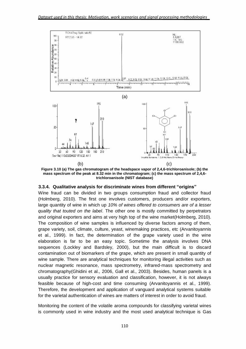
3.3.3. Feasible study for detection of 2,4,6-tirchloroanisole (2,4,6-TCA) in wine

using a portable Ni-IMS.

Wine industry has a high impact in the Spanish economy. Actually, Spain is the third

biggest producer in Europe and Spaniards are the ninth wine consumers in the world

according to International Organization of Wine and Vine. Hence, Spanish producers

devote much attention about the wine production and make an effort to control any

process that can alter wine quality. In this context, Trichloroanisole (TCA), particularly

the 2,4,6-TCA isomer, is commonly identified as the main compound responsible for

the off flavor of wine known as "cork taint".

TCA can migrate from cork stopper to the wine producing changes in the organoleptic

properties reducing wine quality (Rubio-Coque et al., 2006, Pereira et al., 2000,

Sefton and Simpson, 2005). Other isomers of trichloroanisole, substituted tetra- and

penta- chloro-anisoles and compounds such as tribromoanisole, 2-methylbornoleol,

4-ethylguaiac, etc., were also associated with off flavor of wine. Furthermore, the use

of the common term "cork taint" is misleading as it attributes the origin of the

unpleasant aroma of tainted wine to the cork alone, while in fact the odorous

compounds may originate from the wood in barrels used for aging wine (especially

reusing barrels that have been cleaned), wooden structures within the vineyard and

traces of TCA were even detected in water (Sefton and Simpson, 2005, Rubio-Coque

et al., 2006). However, 2,4,6-TCA originating from cork material is still being


105

considered as the main source for tainted wine that effect wine producers globally

and the financial losses are estimated in the range of 1-10 billions US-dollars

annually(Rubio-Coque et al., 2006).

(Buser et al., 1982) were the first researchers who attributed the off-flavor of wine to

2,4,6-TCA and since then several publications have confirmed the effects of the

presence of this compound on the wine flavor (Fischer and Fischer, 1997, Pereira et

al., 2000, Teixeira et al., 2006). The human olfactory threshold for 2,4,6-TCA in wine

(in the liquid phase) is usually well below 10 ng L-1 and in one study it was estimated

to be 2.1 ng L-1 and the customer rejection level was only slightly higher at 3.1 ng L-1

(Prescott et al., 2005).

The consumers of wine usually describe TCA as wet cardboard mushrooms, earthy

smell, etc.(Mazzoleni and Maggi, 2007) and the origin of these compounds in wine

was attributed mainly to the presence of chlorine substituted compounds, including

chlorophenol derivatives, in the cork stopper material and sometimes to the content of

similar chemicals in wood barrels, especially cleaning materials deployed for re-use of

these barrels for aging of the wine. The dominant mechanism for production of 2,4,6-

TCA, that is not a naturally occurring compound, is usually described as O-

methylation of 2,4,6-trichloro-phenol (2,4,6-TCP) by filamentous fungi(Maggi et al.,

2008, Prak et al., 2007). TCP and pentachlorophenol are widely used as pesticides in

agriculture and other applications including sanitizing wood products.

Several analytical approaches have been adopted in order to provide an objective

measure for the concentration of the compounds responsible for the "tainted" wine

flavor (Riu et al., 2006, Riu et al., 2007, Bianco et al., 2009, Zalacain et al., 2004,

Pizarro et al., 2012, Weingart et al., 2010, Fontana et al., 2010, Luisa Alvarez-

Rodriguez et al., 2009, Vlachos et al., 2007, Alzaga et al., 2003). The most common

methods deploy solid phase microextraction (SPME) fibers to pre-concentrate TCA

from the headspace vapor phase or from the wine itself that is generally combined

with stir-bar agitation. The pre-concentration step is generally followed by gas

chromatographic (GC) separation of the components of the wine or headspace

vapors that were adsorbed on the SPME fiber. Finally detection of the GC effluent is

carried out by electron capture detectors (ECD) or more commonly by different mass

spectrometric instruments that also identify the components. The reported limit of

detection (LOD) for 2,4,6-TCA by these methods is generally in the 1-100 ng L-1

range after pre-concentration.

As it was pointed out in introduction, Ion mobility spectrometry (IMS) is a well-

established method that is frequently used for detection of hidden explosive,

contraband drugs and monitoring the presence of toxic chemicals in ambient air

(Eiceman and Karpas, 2005). Recently applications in the fields of medical

diagnostics and food quality have been developed. Among these are monitoring

processes of beer fermentation (Vautz et al., 2004), determining the spoilage and

freshness of muscle food products (Karpas et al., 2002b) and detection of molds

(Ruzsanyi et al., 2003). These applications take advantage of the fact that IMS has a

high sensitivity for compounds with high proton affinity or high electro-negativity

values and that the ion chemistry can be controlled to enhance the response to the

target analytes while avoiding interferences from many other chemicals that may be


106

present in the matrix. Several chlorophenol derivatives have been studied by liquid

chromatography followed by electrospray ionization and ion mobility spectrometry

(LC-ESI-IMS) (Tadjimukhamedov et al., 2008). In a couple of recent publications by

Marquez-Sillero et. al., 2,46-TCA was determined in water and wine samples by ionic

liquid-based single-drop micro-extraction and ion mobility spectrometry (Marquez-

Sillero et al., 2011a, Marquez-Sillero et al., 2011b). The limit of detection that was

reported, 0.2 ng L-1 (Marquez-Sillero et al., 2011a) or 0.01 ng L-1 for a 2 mL wine

sample(Marquez-Sillero et al., 2011b), appears to have considerably superseded all

other methods. These results showed the potential use of IMS as technique of TCA

screening, provided a pre-concentration instrument is used such as single-drop micro

extraction technique. Nevertheless, the measuring time is slightly high, around 40

minutes, which reduce the likelihood of introducing IMS in the vineyard market as

detection instrument of TCA.

The main objective of the current work was to study the atmospheric pressure gas-

phase ion chemistry of 2,4,6-trichloroanisole that pertains to IMS in positive and

negative modes and to determine the limit of detection of IMS for 2,4,6-TCA. This is

also the first study of the potential of a stand-alone IMS for direct determination of

TCA without GC pre-separation or other method for preconcentration. Based on these

results we assess the potential for using this technique to monitor off flavor in wine.


2,4,6-trichloroanisole (TCA) (CAS 87-40-1) was purchased from Aldrich (lot

#MKBG3491V) and used without further purification after its purity was tested with

GC-MS (see below). Headspace vapor vials with a volume of 20 mL sealed with 20

mm crimp and 20 mm PTFE/silicone septum3 (all from ChemLab, Barcelona) were

used throughout the study. Stock solutions were prepared by weighing samples of

TCA and dissolving them in dichloromethane (DCM, CAS 75-09-2, Fluka 66750,

98%) or in ethanol (99.5%, Panreac Sintesis, Barcelona) yielding concentrations of

2.03 and 2.89 µg µL-1, respectively. The DCM stock solution was diluted tenfold to

produce a solution with 0.2 µg µL-1.

Duplicate samples of TCA, containing 2 to 40 µg, were prepared by pipetting a known

volume of the stock solution, or diluted solution, on a piece (about 5x3 mm) of filter

paper (Fisherbrand code 1490) that was placed in a headspace vial. The vial was

sealed immediately after the solution was deposited on the filter paper to avoid loss of

the solvent and analyte. After at least five minutes at room temperature (about 25ºC)

for evaporation and equilibration the vial was inserted into a homemade aluminum

heater that was kept at 100ºC for two minutes in order to vaporize the sample. The

temperature in the center of the top part of the vial was about 70ºC. At that time two

needles pierced the septum: one was connected to a tube that carried a 400 mL min-

1 stream of purified air, or air seeded with dichloromethane as a dopant, and the

other needle was connected through a short piece (about 10 cm) of 1/8” Teflon tubing

to the IMS. It was assumed that absorption of TCA vapor on the surface of the tubing

would be minimal due to the high flow rate through the narrow tube.

An additional stock solution containing 15 µg µL-1 of 2,4,6-TCA in ethanol was also

prepared and a 25 µL aliquot (containing 375 µg of TCA) was added to 225 µL of

white wine or red wine. A blank sample was prepared by adding 25 µL of pure ethanol


107

to 225 µL of wine. Each sample was placed on a 55 mm diameter filter paper and

allowed to evaporate to dryness in a hood and then folded and placed in a headspace

vapor vial that was sealed. Analysis of these sealed vials was carried out as

described above.

In addition, 8.5 mg of 2,4,6-TCA were placed inside a 20 mL headspace vial that was

sealed. Taking 2.065 Pa as the vapor pressure of TCA at 25ºC 27, the amount of

TCA vapors in 20 mL at equilibrium was calculated as 5.45 µg and this served as

means to estimate the sensitivity of the system. Exponential dilution could not be

carried out with this system as only a fraction of the 2,4,6-TCA was vaporized.

The ion mobility spectrometer used was the handheld Gas Detector Array 2 (GDA2,

Airsense Analytics, Germany). The instrument was switched on and allowed 30

minutes for stabilization before measurements began. The operating temperature of

the drift tube was 44ºC. The sampling airflow was set at 400 ml min-1 and the

measurements were made with no internal dilution of the sample.


In order to obtain a quantitative model for the correlation between the response of the

IMS and the TCA concentration, a number of signal processing steps are needed. A

main characteristic of IMS spectra is the presence of several ion species from the

same analyte with different dependencies on the analyte concentration. The

procedure described below allows consideration of all ion peaks with the proper

weight automatically assigned in the model building procedure. Additionally, the

proposed signal processing chain takes into account the full set of spectra from every

individual sample.


108

Figure 3.9 Block diagram of signal processing for TCA samples

A block diagram of the signal processing procedure is shown in Figure 3.9. The main

blocks are: (i) spectra pre-processing (ii) spectra resolution by MCR-

LASSO(Pomareda et al., 2010) and (iii) multivariate calibration by Partial Least

Squares. To estimate the limit of detection (LOD) and limit of quantification (LOQ) a

set of four blanks was taken separately and used uniquely for the purpose of LOD

estimation and the dataset to train the model was comprised of 15 samples with 0 to

40 g of TCA deposited on the filter paper. All the spectral signal processing, as well

as the estimations of LOD and LOQ was performed using the negative polarity

spectra of the IMS that were measured with dichloromethane as a dopant.

Once spectra has been preprocessed, multivariate curve resolution (MCR-LASSO

(Pomareda et al., 2010))was applied to the data matrix yielding a spectra profile. The

number of pure compounds was selected to be three by visual inspection of the

spectra. The technique also provides the concentration profiles for every individual

peak along the sample transient, in this case consisting of 15 samples that contain 13

spectra each one.

Quantification based on MCR results has been previously considered (Antunes et al.,

2002). In the present study, a partial least squares model was built based on the

concentration profiles. The input pattern for each sample consisted in the

concatenation of the concentration profiles for two ionic species related with TCA

monomer and dimer ions. The dimension of this vector is 26 (13 spectra x 2 pure

components) to each sample that give at the end a matrix of dimension 15 samples x

26 concentration profiles. PLS model order was decided by cross-validation


109

procedure (leave one out) optimizing the RMSECV (root mean square error cross-

validation).

Once the model had been built, four blank samples, which were measured

separately, were projected over the calibration model, and their predicted value was

used to estimate LOD and LOQ. The limit of detection and limit of quantification

determination was carried out in accordance with IUPAC (Mocak et al., 1997) Eq. 3.6.

GC-MS measurements

The purity of the 2,4,6-TCA was determined from GC/MS (Focus GC with DSQ II

mass spectrometer, Thermo Scientific) measurements of the headspace vapor

emanating from a sample of 47 mg that was placed in a 20 mL vial that was

hermetically sealed with a PTFE/silicone septum. The sample was thermostatted for

10 min at 100ºC under constant stirring. Afterwards, 1 mL of the headspace vapors

was introduced into the injector port of the gas chromatograph. Chromatographic

injection was made in split mode (1:50) at 250ºC. A TRB-5MS chromatographic

column (30m x 0.25mm i.d., 0.25µm film thickness) was used with an oven

temperature program of 60ºC (2 min) at 20ºC min-1 up to 260ºC (2 min). The carrier

gas was high-purity helium with a flow-rate of 1.0 mL min-1. Mass spectra were

recorded by electron impact (EI) ionization at 70eV and ion source temperature of

200ºC.

A single peak appeared in the gas chromatogram with a retention time of 8.32 min

Figure 3.10 (a). The mass spectrum corresponding to this peak is shown in Figure

3.10 (b) that displays the mass spectrum of 2,4,6-TCA obtained in full scan mode

(mass range 35-350 Da). Identification of TCA was confirmed through the comparison

of the NIST-library mass spectrum of TCA Figure 3.10(c) with the mass spectrum

obtained from the sample. The ions around m/z 210 are attributed to the

quasimolecular ion with typical isotopic pattern of three chlorine atoms, while the ions

around m/z 195 represent the same pattern after the loss of the methyl group.


110

(a)

(b)

(c)

Figure 3.10 (a) The gas chromatogram of the headspace vapor of 2,4,6-trichloroanisole; (b) the mass spectrum of the peak at 8.32 min in the chromatogram; (c) the mass spectrum of 2,4,6-

trichloroanisole (NIST database)

3.3.4. Qualitative analysis for discriminate wines from different “origins”

Wine fraud can be divided in two groups consumption fraud and collector fraud

(Holmberg, 2010). The first one involves customers, producers and/or exporters,

large quantity of wine in which up 10% of wines offered to consumers are of a lesser

quality that touted on the label. The other one is mostly committed by perpetrators

and original exporters and aims at very high top of the wine market(Holmberg, 2010).

The composition of wine samples is influenced by diverse factors among of them,

grape variety, soil, climate, culture, yeast, winemaking practices, etc (Arvanitoyannis

et al., 1999). In fact, the determination of the grape variety used in the wine

elaboration is far to be an easy topic. Sometime the analysis involves DNA

sequences (Lockley and Bardsley, 2000), but the main difficult is to discard

contamination out of biomarkers of the grape, which are present in small quantity of

wine sample. There are analytical techniques for monitoring illegal activities such as

nuclear magnetic resonance, mass spectrometry, infrared-mass spectrometry and

chromatography(Ghidini et al., 2006, Gall et al., 2003). Besides, human panels is a

usually practice for sensory evaluation and classification, however, it is not always

feasible because of high-cost and time consuming (Arvanitoyannis et al., 1999).

Therefore, the development and application of vanguard analytical systems suitable

for the varietal authentication of wines are matters of interest in order to avoid fraud.

Monitoring the content of the volatile aroma compounds for classifying varietal wines

is commonly used in wine industry and the most used analytical technique is Gas


111

Chromatography techniques (Pedro Santos et al., 2010, Lozano et al., 2005, Kataoka

et al., 2000, Yamamoto et al., 1982, Ferreira et al., 2000). There are other analytical

techniques used for classifying wines, among of them Ultra High Resolution Mass

Spectrometry (Cuadros-Inostroza et al., 2010), electronic noses and electronic

tounge(Legin et al., 2003, Buratti et al., 2004). The uses of sensors as electronic

noses or artificial olfactory systems try to imitate a simplified human sense of smell

but removing the subjective component implicit in it. These systems have the

advantage of high portability for in situ and on-line measurements with lower cost

(Lozano et al., 2005). Also they have high sensitivity, fast response, easy operation

and capability to recognize different volatile compounds profiles. In this sense, IMS

technique could be an alternative and appropriate sensor for the characterization and

classification of different types of wines. On the other hand, wines could be potential

products for frauds in the international market (Holmberg, 2010) . For this reason, it is

necessary to develop easy and reliable analytical tools to control the characteristic of

each wine and to confirm the information of their labels.

Moreover IMS equipment is very versatile and therefore different sample introduction

systems (SIS) are an essential supplement for introducing volatile analytes in an

efficient way into the IMS equipment. Different SIS coupled to IMS are described in

the bibliography(Arce et al., 2008) and this SIS are characterized by their simplicity

and low cost to get profit of the IMS technique(Menendez et al., 2008, Alonso et al.,

2008).

The main goal of this work is to perform a classification model using the whole

spectra for discriminate the wine samples by their origin. In this case a new sampling

technique called Gas Phase Separator (GPS) for in-line introduction of volatile

analytes present in liquid samples was used coupled to UV-IMS. In this case, it has

been used for the extraction and injection of volatile analytes presents in wine

samples and the classification of different types of white wines using their volatile

analytes profiles. Multivariate statistical techniques are going to be used to extract

and use information based on the overall properties of the sample and perform a

classification without the need for additional compositional data. In addition, a robust

cross-validation methodology was implemented in order to assure the effectiveness of

the model and classification.

Methods and Sample Preparation

Wines samples from four different origins, which were selected due to their similar

organoleptic characteristics, were analyzed using UV-IMS. Each sample was

continuously recorded for about 2 minutes. The wines brand of origin used in this

work were: Montilla-Moriles (n=15), Jerez (n=13), Valdepeñas (n=16) and Condado

de Huelva (n=12). The wine samples were stored in their original container at ambient

temperature, while this work took place.

The manifold employed for the in-line vapour phase generation and mobility

measurements is depicted in Figure 3.11. The SIS selected in this work was used by

Armenta et al. (Armenta et al., 2006) for seafood freshness determination using

Fourier Transform Infrared (FTIR) spectroscopy. The SIS consisted in a peristaltic

pump of four channels, furnished with Teflon tubes, which was used to introduce the


112

wine samples in the flow system. The connections and reaction coils were made from

Teflon tubing. The gaseous phase was separated from the liquid stream in a home-

made Pirex-glass of 4.7 mL volume GPS. The manifold incorporates an oven to

improve the removal of volatile compounds from wine samples.

Wine samples were continuously aspirated inside the manifold of Figure 3.11 at 0.7

ml min-1 flow. Wine samples were passed through a 100 cm length coil heated at

80ºC and introduced in the GPS from which the generated volatile compounds were

transported to the UV-IMS equipment after 15 min of generation of volatile

compounds using a N2 carrier flow of 20 ml min-1. During these 15 min, the stream of

highly pure nitrogen (6.0) from Abelló Linde (Barcelona, Spain) was passed through

the UV-IMS system for cleaning and stabilization while drift gas (N2) pass in

crosscurrent to a flow of 70 ml min-1.

Figure 3.11 Introduction system of wine samples using UV-IMS (Garrido-Delgado et al., 2011a).


The signal processing consists of pre-processing spectra following with a step of

outlier detection to reject those samples that do not fit in the model. The signal

processing is explained in detail in chapter four, but the main idea is to noise

reduction, baseline correction and alignment. Since any dopant was present in the

samples, the alignment was done taken a reference spectrum for all samples. The

following focus was to build a robust model whose accuracy get been maximized. A

representation of the main blocks for signal processing of this work is shown in Figure

3.12.


113

Figure 3.12 Block diagram of the analysis of wine samples for classification purposes.

Briefly, the spectra were cut, which was from 15.4 to 27 ms, in order to analyze

spectra where the main information was located. The outlier detection was based on

Q statistic and T2 analysis, thus spectra and entire samples were discarded when the

Q and T2 statistic were higher than 95% of the confidence limit. The model proposed

in this work is a combination of principla component analysis (PCA) and linear

discriminant analysis(LDA) (Wang et al., 2004)and the final classification was based

on the results provided by kNN classifier.

PCA (Bishop, 2006) is a signal processing technique that generates projections along

the directions of maximum variance of the analyzed data. It has also been used as an

unsupervised technique to beat the course of dimensionality generating projections of

the original data in a reduced dimension where the maximum variance is preserved.

LDA (Bishop, 2006)is a signal processing technique that maximizes class

separability, generating projections where the examples of each class from compact

clusters and the different clusters are far from each other. LDA has been used as

supervised linear projection technique to find directions of maximum separation from

a set of samples for which class membership is known in order to be able to predict

the class membership of unknown samples.


114

The kNN (Henley and Hand, 1996, Denoeux, 1995) method is a technique used to

generate nonlinear classifications, finding the closest k examples in the dataset to the

unknown class, and selecting the predominant class for it. kNN has been used for the

classification of the wine samples in their correct group. The model is built based on a

training set; later, it is used to predict classes of new samples (validation set). In this

work, k equal to 3 was used.

Bootstrap validation (Felsenstein, 1985, Efron, 1979)was proposed in this work for

avoiding overfitting results. Bootstrap validation procedure allows resampling the data

set with replacement, to generate sets of observations that may be used for the

estimation of statistic magnitudes as the performance of the model.

3.3.5. Feasible study for measurement potential biomarkers of Prostate Cancer

using Ion Mobility Spectrometry

Volatile organic compounds present in both breath and bodily fluids have been

studied by virtue of its potential use as non-invasive diagnosis tool in medical

applications. In fact, a number of VOCs in breath have been recognized as

biomarkers for several systemic diseases and monitoring purposes. Acetone in breath

is totally linked to patients with uncontrolled diabetes mellitus (Lebovitz, 1995),

elevated ammonia is linked to patients with renal failure (Davies et al., 1997) and

propofol levels can be used for monitoring anaesthesia in clinical use (Perl et al.,

2009). Nevertheless, the study of VOCs in urine has received much less attention

than breath samples. One of the major studies was undertaken by Mills and Walker

(Mills and Walker, 2001) in which 103 compounds where found from 5 heterogeneous

patients at different conditions using SPME-GC/MS as analytical technique. There

have been other studies in healthy individuals giving as a result potential biomarkers

present in elderly population (Smith et al., 2008).

Since, urine is routinely used in diagnostics of diseases as diabetes mellitus and

urinary tract infections, its potential as diagonistic tool for detecting cancer is really

noteworthy. There have been some studies in liquid-chromatography for detect

presence of non-volatiles as biomarkers for melanoma metastases (Yamada et al.,

1992). The volatiles in urine cover a range of chemical classes, among of them,

acids, alcohols, ketones, aldehydes, amines, sulphur compounds and hydrocarbons

(Costello and Ratcliffe, 2013). Indeed, ketones have been reported to be linked to

bacterial action in the gut , and some aliphatic amines have been observed during

hepatic and renal diseases (Mitchell and Zhang, 2001).Although it is still unclear the

cellular and biochemical origin of endogenous VOCs metabolites released to urine as

consequence of a neoplasic lesion, some experimental works have related an

increase of formaldehydes with bladder and prostate cancer patients (Spanel et al.,

1999). However, no compound or set of compounds have been proposed as serious

candidates for bladder or prostate cancer clinical diagnostics.

Prostate cancer (PCa) is the third leading cause of death from cancer in men in the

European Union. PCa can be treated by various therapies if only it is detected in its

initial stages. The suspicion of PCa is established through elevated serum PSA

(prostate-specific antigen) and/or DRE (digital rectal exam), and its diagnosis is

confirmed through prostate biopsy As a consequence of the current screening

parameters, large populations of men with chronically elevated PSA undergo

repeated biopsies to rule out PCa (Loeb et al., 2009, Pannek and Partin, 1997).


115

Around ⅔ of the approximately 1.300.000 biopsies made yearly in Europe are

negative and therefore unnecessary. Therefore, other alternatives are needed that

can help to an early diagnosis and identify patients whit high risk of developing PCa

from whom repeat prostate biopsies should be mandatory. As prostate cells can be

detected in the urine of men with PCa, urine-based diagnostic tests have the

advantage of being non-or minimally invasive. Recently, urine has been extensively

analyzed by proteomics, revealing that more than 1,500 proteins constitute the

normal urine (Adachi et al., 2006). The origins of the proteins found in the normal

human urine are plasma proteins (≈ 30%) and other proteins (≈ 70%) secreted by the

bladder or the prostate gland into the urine (Oh et al., 2004, Pieper et al., 2004,

Thongboonkerd et al., 2002).

In a previous study urine sample were analyzed using headspace GC/MS. The urine

sample were taken from subjects with PSA levels (>4.0 ng/ml) and/or an abnormal

diagnostic DRE and healthy subjects. After the data analysis, a subset of volatiles

was found as potential biomarkers correlated with PCa patients. From the results one

of the compounds, which are going to be known as Compound A, seems to be

preferable present in patient with PCa than healthy subjects. Thus, the aim of this

work is to test two commercial spectrometers as potential portable device for

detection of PCa in clinical use. A set of measurements at different concentrations

were carried out for continuous monitoring of a stream of air/nitrogen with a given

concentration of the analyte and headspace vapors in a sealed vial to determine the

response of the spectrometers to the compound A mixed with milliQ water. The limit

of detection of the Compound A in air-gas phase and headspace is going to be

calculated for the two commercial spectrometers.


Compound A was purchased from Sigma-Aldrich (Madrid, Spain). A sample of the

compound was inserted in a permeation tube that was placed in an oven with

controlled chambers at 30ºC (Owlstone OV4, UK). The permeation tube was

periodically weighted to determine the amount of the sample that emanates from the

tube. The concentration was determined by the oven temperature and permeation

rate of the compound. Table 3.7 shows the concentrations that were introduced to

both spectrometers. The airstream was introduced by Teflon tubing to the inlet port of

each device. The response was measured and a limit of detection to vapors was

derived from the calibration curve.


116

GDA2 (400 ml min-1) UV-IMS (50 ml min-1)

Airstream (ppm) Headspace(µg ml-1) Airstream(ppm) Headspace(µg ml-1)

0.6 5 0.6 0.1

2 10 2 0.5

4 20 4 1

6 50 6 2

8 100 8 5

10 250 10 10

12 500 12 15

14 - 14 20

16 - 16 25

18 - 18 50

20 - 20 75

22 - 22 100

24 - 24 125

- - - 150

Table 3.7 Range of concentrations of Compound A for both spectrometers.

For the headspace measurements, a stock of solution of Compound A was prepared

in ultrapure milli-Q water at a concentration of 812 mg l–1 and stored at 4 ºC. Working

standard solutions were prepared on a daily basis by rigorous dilution of the stocks in

ultrapure milli-Q water. The introduction of the sample into the spectrometers was

carried out through a loop flow path 4-ports valve. Two ports of the valve were

connected to two stainless steel needles for the subsequently introduction into the

headspace of a sealed vial. Another connection of the valve was coupled to the

source of purified air/nitrogen stream and the other port was connected to the sample

inlet of the instrument, as shown in Figure 3.11. Connections were made through 1/8"

OD PTFE tubing.

The process for generating the headspace of the sample and the subsequent

introduction into the instrument was as follows: 10 ml of an aqueous solution

containing a known concentration of Compound A was spiked in a glass vial of 20 ml,

which was tightly fitted with a removable aluminum cap provided with a silicone

septum. Then, the sample introduction system was set in “extraction” mode (Figure

3.13(a)) in which the needles were injected into the headspace of the vial.

Subsequently, the vial was heating at 40 °C for 15 min to allow the passing of the

Compound A to gas phase. Once this time was elapsed, the switch of the valve was

rotated to change the system to the “injection” mode (Figure 3.13 (b)). Thus, the

headspace generated in the vial was dragged by a stream of highly purified

air/nitrogen and directly introduced into the spectrometer for the analysis. The start of

data collection was coordinated with the change to "injection" mode position of the

valve. The carrier flow through the headspace vial was 400 ml min-1 for the GDA2 and

50 ml min-1 for the UV-IMS. The concentrations range for headspace is shown in

Table 3.7.


117

a) Extraction mode b) Injection mode

Figure 3.13 Sample introduction system used to generate and inject the sample into the UV-IMS instrument.


The procedure for the limit of detection calculation is similar to that explained in

section 3.3.2 and Figure 3.9. The preprocessing step is specific for each

spectrometer (see chapter four), but the main idea is to get a clean spectra in order to

obtain accurate results.

The first step is going to determine the reduced mobility coefficient (K0) of pure

analyte. Then MCR-Lasso is going to be used for extract the pure compound and use

the concentration profile for calibration purposes. The limit of detection is going to be

determined using blanks that were taken in each experiment. At the end, a qualitative

and quantitative analysis is going to be carried out to figure out the use of IMS for

PCa detection.

3.3.6. Breath analysis for detection of SEPSIS in rats using Ion Mobility

Spectrometry

Thanks to the pioneering work of Pauling, it has been known since the 1970s that

human breath is a complex mixture of hundreds of compounds (Teranish.R et al.,

1972, Pauling et al., 1971). Gas Chromatography-Mass Spectrometry has made it

possible to identify some of these compounds, revealing that exhaled breath included

traces of many volatile organic compounds (VOC), small inorganic molecules and

non-volatile substances such as isoprostanes, cytokines or leukotrienes (Smit et al.,

To UV-IMS From nitrogen source To UV-IMS From nitrogen source


118

2007, Westerhuis et al., 2008, Miekisch and Schubert, 2006). Accordingly, there is

now a consensus about the diagnostic potential of breath, and there is considerable

evidence available to support the use of breath analysis as a diagnostic tool for

pulmonary diseases, liver diseases, gastric diseases, diabetes and inflammatory

diseases such as sepsis (Miekisch and Schubert, 2006, Sethi et al., 2013, Phillips et

al., 2010, Vautz et al., 2010a, Zhang and Li, 2010, Smith and Spanel, 2007). The

analysis of exhaled breath has a number of advantages compared with traditional

diagnostic techniques: it is a non-invasive, painless procedure that does not require

skilled medical staff (Buszewski et al., 2007).

Despite this undeniable interest, however, only a few breath tests, such as

capnography and the urea breath test, are typically used in clinical routine. One

reason for the continued reluctance to use breath analysis as a common diagnostic

tool in clinical practice is lack of knowledge about the compounds' metabolic

pathways of the compounds, although another factor is the lack of normalization and

standardization methods (Miekisch and Schubert, 2006). Furthermore, bedside

systems are not always compatible with the sophistication now required of analytical

instruments. Gas chromatography-mass spectrometry (GC/MS), for example, is the

most widely used instrument in breath analysis (Van Berkel et al., 2010, Phillips et al.,

2007, Phillips et al., 1999) but, although it offers very good sensitivity, precision and

resolution, the sampling procedures and subsequent interpretation of data can be

demanding and time-consuming and require qualified personnel.

Promising results of breath analysis with IMS have been reported and its potential for

application as a diagnostic instrument is huge. Lung cancer has been the main focus

of attention (Vautz et al., 2013, Carstens et al., 2010, Vautz et al., 2010a, Marcus et

al., 2012, Sobel et al., 2012) but also interesting findings have also emerged with

respect to COPD, sarcoidosis (Bunkowski et al., 2009b) and vaginitis (Chaim et al.,

2003, Karpas et al., 2002a). Other diseases such as sepsis have yet to be tested by

IMS technology, however, even although the potential capability of breath test for the

diagnosis of sepsis has been posited in some works (Miekisch and Schubert, 2006).

Sepsis is a clinical condition characterized by systemic inflammation, aberrant

immune response, and microcirculation/coagulation disorders generated by the host

in combating an infection due to bacterial toxins absorbed from infected wounds and

passed into the bloodstream (Opal, 2014). It is a common cause of morbidity and

mortality in elderly, immuno-compromised and critically ill patients, and it is the

commonest cause of death in adult intensive care units (Parker and Watkins, 2001).

Several rodent models have been used for sepsis studies in various works (Schultz

and van der Poll, 2002, Tarkowski et al., 2001) and, although the correlation between

animal and human models is not perfect, rat models can make a positive contribution

in many areas, such as the reduction and standardization of experimental variability

and the simplification of the experimental setup. One of the common sepsis models

used in murine is the induction of sepsis through an exogenous bacteria infection. It is

well known that mimicking bacterial infection by using lipopolysaccharide (LPS),

which is a structural component of gram-negative bacteria, has been used as a model

to activate the immune system, inducing fever, sepsis and multi-organ injury (Lava et

al., 1982). The main cytokines acting as endogenous pyrogens in response to LPS


119

are interleukin (IL)-1β, IL-6 and tumor necrosis factor-α (TNF-α). Moreover,

pulmonary dysfunction, including edema, is a well-recognized dysfunction in sepsis

(Sethi et al., 2013, Sethi et al., 2008).

The analysis of exhaled breath in rats has been reported in some studies (Vautz et

al., 2010b, Weicker et al., 2001, Dercho et al., 2006) and the analysis of rodent’s

breath with an IMS instrument has been reported in a recent feasibility study by Vautz

et al (Vautz et al., 2010b).

This work explores the viability of the IMS instrumentation and chemometric

techniques to generate a VOC discriminatory pattern of sepsis through breath

sampling. This work has been performed in a rat model as a first step towards a

possible future application in humans. Furthermore, although IMS is undoubtedly

capable of providing fast VOC analysis, it also needs to be compared with a gold

standard technique in VOC analysis. In order to fill this gap, this study includes

GC/MS measurements of the rat’s breath as a reference technique, while also

providing analyte identification capabilities using proper MS libraries.


This study was carried out on 20 Sprague-Dawley male rats from Charles River (250-

300g) following an experimental protocol approved by the Ethical Committee of

Animal Research at the University of Barcelona. One day before the experiment, 10

of these rats were intraperitoneal (IP) injected with LPS from Escherichia coli 055:B5

(Sigma Chemical Co., St. Louis, MO) at a concentration of 4mg/kg and the other 10

rats were IP injected with saline solution as a control group. All the animals were

housed in light-dark cycle-regulated air conditioned (23ºC) and air humidity (60%)

animal quarters for 24h. After this period, the animals were IP sedated and

anaesthetized with a mixture solution containing Rompun (Bayer) in a concentration

of 0.7mL/kg and Imalgene 1000 (Merial Laboratories, Spain) in a concentration of

1mL per kilogram of animal body weight. A tracheotomy was performed and one

cannula (16GA BD Adsyte Pro, Becton Dickinson, Spain) was introduced into the

trachea. The intratraqueal cannula was connected, by means of a T-piece, to the

inspiratory and expiratory lines of a conventional mechanical ventilator (Harvard,

USA). The rats were ventilated normally, with a tidal volume of 7ml per kg of body

weight, at a rate of 80 breaths/min using room air. The ventilation period lasted for 20

min and at the end of this period the expiratory gas was sampled for further VOC

analysis. Figure 3.14shows the sampling method used in this work. With GC/MS the

rat's breath was collected in a perfluoralkoxy (PFA) bag for subsequent analysis. With

IMS, the breath sample is directly introduced into the instrument via the expiratory line

and measured online.


120

Figure 3.14 Experimental setup of breath sampling (Guaman et al., 2012).

After expiratory gas sampling, the rats were sacrificed by aortic exsanguination. The

rats' septic status as a result of the bacterial-LPS injection was investigated by

assessing lung edema and systemic inflammation. To assess lung edema, the lungs

of all the rats were excised, quickly weighed after removing the main airways,

weighed (wet weight=W), dried at 70ºC for 48h and weighed again (dry weight=D).

The ratio W/D was computed as a conventional index of lung edema.

The systemic inflammatory status of the rats injected with LPS was determined by

measuring the plasma concentrations of two representative inflammatory cytokines:

IL1-β and TNF-α. To this end, the peripheral blood was processed to isolate the

plasma (centrifugation at 3,000 g using a vasculant rotor for 15 min at 4 ºC). Enzyme-

linked immunosorbent assays (ELISA) for IL1-β and TNF-α were performed

(Quantikine, R&D Systems, Minneapolis, MN, USA).

The IMS used in this study was the GDA2 (Airsense Analytics, Germany) which

measurements were made at 50% internal dilution of sampling, with a sampling flow

of 200ml/min. All the samples were measured twice for up to 40s after 5min of

stabilizing the system and IMS. Once these measurements with the IMS were

finished, 1L of breath was collected in PFA bags (Jensen Inert Products, USA) for

subsequent SPME-GC-MS analysis.

The GC/MS analyses were performed on a Focus GC-DSQ II (Thermo Scientific,

USA) with a split/splitless injector. Breath was collected in 1L PFA bags and analyzed

with SPME-GC-MS. A Carboxen/Polydimethylsiloxane (CAR/PDMS) 75-µm-thick fiber

from Supelco was used for the pre-concentration of the analytes. The sorption

conditions were 30min at room temperature. The desorption of volatiles from the fiber

was undertaken at 250ºC for 5min at the GC/MS injection port. A 60m x 0.32mm x

1.8µm capillary column DB-624 (Agilent Technologies) was chosen for the

chromatographic separation. Helium was used as carrier gas, with a flow rate of

1ml/min. The MS analyses were carried out in a full scan mode (scan range 35-


121

350amu) with ionization energy of 70eV. The oven program temperature was as

follows: initially, 40ºC held for 5 min, then ramped 10 ºC min-1 to 180ºC; held for 1

min, then ramped 15ºC/min to 230ºC; and then held for 10min.

At the beginning and at the end of each session of measurements, the blanks of the

sampling system and the air of the laboratory were measured with IMS in order to

ensure the reproducibility of the measurements. In order to counteract the anesthetic

drugs in the ion mobility spectra and in the chromatogram, these products were

measured in a head-space mode by IMS and by SPME-GC-MS.


The signal processing used in this work is shown in Figure 3.15. The signal

processing applied to the IMS dataset was designed to find differences between

healthy and diseased rats, and the signal processing applied to the GC/MS dataset

focused on identifying compounds that could be potentially useful as sepsis

biomarkers.

Figure 3.15 Block diagram of the analysis of vapors from breath analysis for determining SEPSIS in rats.

The IMS dataset have to be pre-processed as it has been explained above (3.2.1).

The multivariate signal processing strategy involved the use of the iterative algorithm

MCR-LASSO (Pomareda et al., 2010) to estimate the pure contributions to the

spectra. The spectra profile and concentration profile are likely to be linked to the

biomarkers of breath, thus the specific biomarkers of sepsis. Sequential Floating


122

Feature Selection (SFFS) (Pudil et al., 1994, Narendra and Fukunaga, 1977) to select

the best subset of pure contribution for maximum discrimination between classes

using the concentration profile results, and a kNN classifier (Denoeux, 1995, Bezdek

et al., 1986)in the reduced space to evaluate the classification results under a

bootstrap validation (Felsenstein, 1985, Efron, 1979)strategy.

As regards the GC/MS dataset, the compounds were identified by comparison with

mass spectra from the NIST 2005 library database available in the Thermo Xcalibur

data system. The basic multivariate strategy involved using a combination of principal

component analysis (PCA) (Bishop, 2006)and linear discriminant analysis

(LDA)(Bishop, 2006) (ref34ref), with a selection based on rank products(Smit et al.,

2007, Breitling et al., 2004). This strategy made it possible to reduce dimensionality

and order the identified compounds by their p-value. A kNN, SFFS and bootstrap

validation were also used in the same way as in the IMS dataset analysis.


123

3.4. Reference

3QBD. 3QBD Israel [Online]. Available: www.3qbd.com/English/ 2012]. Adachi, J., Kumar, C., Zhang, Y., Olsen, J. V. & Mann, M. 2006. The human urinary proteome

contains more than 1500 proteins, including a large proportion of membrane proteins. Genome Biol, 7, R80.

Airsense. 2012. GDA2, Airsense Germany [Online]. Available: www.airsense.com/en/products/gda-2/.

Alonso, R., Rodriguez-Estevez, V., Dominguez-Vidal, A., Ayora-Canada, M. J., Arce, L. & Valcarel, M. 2008. Ion mobility spectrometry of volatile compounds from Iberian pig fat for fast feeding regime authentication. Talanta, 76, 591-596.

. Alzaga, R., Ortiz, L., Sachez-Baeza, F., Marco, M. P. & Bayona, J. M. 2003. Accurate

determination of 2,4,6-trichloroanisole in wines at low parts per trillion by solid-phase microextraction followed by GC-ECD. Journal of Agricultural and Food Chemistry, 51, 3509-3514.

Antunes, M. C., Simao, J. E. J., Duarte, A. C. & Tauler, R. 2002. Multivariate curve resolution of overlapping voltammetric peaks: quantitative analysis of binary and quaternary metal mixtures. Analyst, 127, 809-817.

Arce, L., Menendez, M., Garrido-Delgado, R. & Valcarcel, M. 2008. Sample-introduction systems coupled to ion-mobility spectrometry equipment for determining compounds present in gaseous, liquid and solid samples. Trac-Trends in Analytical Chemistry, 27,

139-150. Armenta, S., Alcala, M. & Blanco, M. 2011. A review of recent, unconventional applications of

ion mobility spectrometry (IMS). Analytica Chimica Acta, 703, 114-123. Armenta, S. & Blanco, M. 2012. Ion mobility spectrometry as a high-throughput analytical tool

in occupational pyrethroid exposure. Analytical and Bioanalytical Chemistry, 404, 635-648.

Armenta, S., Coelho, N. M. M., Roda, R., Garrigues, S. & de la Guardia, M. 2006. Seafood freshness determination through vapour phase Fourier transform infrared spectroscopy. Analytica Chimica Acta, 580, 216-222.

Arvanitoyannis, I. S., Katsota, M. N., Psarra, E. P., Soufleros, E. H. & Kallithraka, S. 1999. Application of quality control methods for assessing wine authenticity: Use of multivariate analysis (chemometrics). Trends in Food Science & Technology, 10, 321-

336. Awan, M. A., Fleet, I. & Thomas, C. L. P. 2008. Optimising cell temperature and dispersion

field strength for the screening for putrescine and cadaverine with thermal desorption-gas chromatography-differential mobility spectrometry. Analytica Chimica Acta, 611,

226-232. Bachrach, U. 2004. Polyamines and cancer: Minireview article. Amino Acids, 26, 307-309.

Bauer, G., Wegscheider, W. & Ortner, H. M. 1991. SELECTIVITY AND ERROR-ESTIMATES IN MULTIVARIATE CALIBRATION - APPLICATION TO SEQUENTIAL ICP-OES. Spectrochimica Acta Part B-Atomic Spectroscopy, 46, 1185-1196.

Bezdek, J. C., Chuah, S. K. & Leep, D. 1986. GENERALIZED K NEAREST NEIGHBOR RULES. Fuzzy Sets and Systems, 18, 237-256.

Bianco, G., Novario, G., Zianni, R. & Cataldi, T. R. I. 2009. Comparison of two SPME fibers for the extraction of some off-flavor cork-taint compounds in bottled wines investigated by GC-HRMS. Analytical and Bioanalytical Chemistry, 393, 2019-2027.

Bishop, C. M. 2006. Pattern Recognition and Machine Learning, New York, NY, Springer Science and Buisness Media.

Bodmer, S., Imark, C. & Kneubuhl, M. 1999. Biogenic amines in foods: Histamine and food processing. Inflammation Research, 48, 296-300.

Bohrer, B. C., Mererbloom, S. I., Koeniger, S. L., Hilderbrand, A. E. & Clemmer, D. E. 2008. Biomolecule Analysis by Ion Mobility Spectrometry. Annual Review of Analytical Chemistry. Palo Alto: Annual Reviews.

Borsdorf, H., Neitsch, K., Eiceman, G. A. & Stone, J. A. 2009. A comparison of the ion chemistry for mono-substituted toluenes and anilines by three methods of atmospheric pressure ionization with ion mobility spectrometry. Talanta, 78, 1464-1475.

http://www.3qbd.com/English/

http://www.airsense.com/en/products/gda-2/

Reference

124

Borsdorf, H. & Rudolph, M. 2001. Gas-phase ion mobility studies of constitutional isomeric hydrocarbons using different ionization techniques. International Journal of Mass Spectrometry, 208, 67-72.

Borsdorf, H., Stone, J. A. & Eiceman, G. A. 2005. Gas phase studies on terpenes by ion mobility spectrometry using different atmospheric pressure chemical ionization techniques. International Journal of Mass Spectrometry, 246, 19-28.

Bota, G. M. & Harrington, P. B. 2006. Direct detection of trimethylamine in meat food products using ion mobility spectrometry. Talanta, 68, 629-635.

Breitling, R., Armengaud, P., Amtmann, A. & Herzyk, P. 2004. Rank products: a simple, yet powerful, new method to detect differentially regulated genes in replicated microarray experiments. Febs Letters, 573, 83-92.

Bro, R. & DeJong, S. 1997. A fast non-negativity-constrained least squares algorithm. Journal of Chemometrics, 11, 393-401.

Bunkowski, A., Bodeker, B., Bader, S., Westhoff, M., Litterst, P. & Baumbach, J. I. 2009a. MCC/IMS signals in human breath related to sarcoidosis-results of a feasibility study using an automated peak finding procedure. Journal of Breath Research, 3.

Bunkowski, A., Bödeker, B., Bader, S., Westhoff, M., Litterst, P. & Baumbach, J. 2009b. Signals in human breath related to Sarcoidosis. — Results of a feasibility study using MCC/IMS. International Journal for Ion Mobility Spectrometry, 12, 73-79.

Buratti, S., Benedetti, S., Scampicchio, M. & Pangerod, E. C. 2004. Characterization and classification of Italian Barbera wines by using an electronic nose and an amperometric electronic tongue. Analytica Chimica Acta, 525, 133-139.

Buser, H. R., Zanier, C. & Tanner, H. 1982. IDENTIFICATION OF 2,4,6-TRICHLOROANISOLE AS A POTENT COMPOUND CAUSING CORK TAINT IN WINE. Journal of Agricultural and Food Chemistry, 30, 359-362.

Buszewski, B., Kęsy, M., Ligor, T. & Amann, A. 2007. Human exhaled air analytics: biomarkers of diseases. Biomedical Chromatography, 21, 553-566.

Cao, L. B., Harrington, P. D. & Liu, J. D. 2005. SIMPLISMA and ALS applied to two-way nonlinear wavelet compressed ion mobility spectra of chemical warfare agent simulants. Analytical Chemistry, 77, 2575-2586.

Carstens, E., Hirn, A., Quintel, M., Nolte, J., Jünger, M., Perl, T. & Vautz, W. 2010. On-line determination of serum propofol concentrations by expired air analysis. International Journal for Ion Mobility Spectrometry, 13, 37-40.

Chaim, W., Karpas, Z. & Lorber, A. 2003. New technology for diagnosis of bacterial vaginosis. European Journal of Obstetrics Gynecology and Reproductive Biology, 111, 83-87.

Choi, S.-S., Kim, Y.-K., Kim, O.-B., An, S. G., Shin, M.-W., Maeng, S.-J. & Choi, G. S. 2010. Comparison of Cocaine Detections in Corona Discharge Ionization-Ion Mobility Spectrometry and in Atmospheric Pressure Chemical Ionization-Mass Spectrometry. Bulletin of the Korean Chemical Society, 31, 2383-2385.

Cirilo, M. P. G., Coelho, A. F. S., Araujo, C. M., Goncalves, F. R. B., Nogueira, F. D. & Gloria, M. B. A. 2003. Profile and levels of bioactive amines in green and roasted coffee. Food Chemistry, 82, 397-402.

Costello, B. d. L. & Ratcliffe, N. M. 2013. Volatile Organic Compounds Found in Urine and Stool. In: Elsevier (ed.) Volatile Biomarkers: Non-Invasive Diagnosis in Physiology and Medicine. Oxford, UK.

Cottingham, K. 2003. Ion mobility spectrometry rediscovered. Analytical Chemistry, 75, 435A-439A.

Cuadros-Inostroza, A., Giavalisco, P., Hummel, J., Eckardt, A., Willmitzer, L. & Pena-Cortes, H. 2010. Discrimination of Wine Attributes by Metabolome Analysis. Analytical Chemistry, 82, 3573-3580.

Davies, S., Spanel, P. & Smith, D. 1997. Quantitative analysis of ammonia on the breath of patients in end-stage renal failure. Kidney Int, 52, 223-8.

de Juan, A., Maeder, M., Martinez, M. & Tauler, R. 2000. Combining hard- and soft-modelling to solve kinetic problems. Chemometrics and Intelligent Laboratory Systems, 54, 123-

141. Denoeux, T. 1995. A K-NEAREST NEIGHBOR CLASSIFICATION RULE-BASED ON

DEMPSTER-SHAFER THEORY. Ieee Transactions on Systems Man and Cybernetics, 25.


125

Dercho, R. A., Nakatsu, K., Wong, R. J., Stevenson, D. K. & Vreman, H. J. 2006. Determination of in vivo carbon monoxide production in laboratory animals via exhaled air. Journal of Pharmacological and Toxicological Methods, 54, 288-295.

Eerola, S., Hinkkanen, R., Lindfors, E. & Hirvi, T. 1993. LIQUID-CHROMATOGRAPHIC DETERMINATION OF BIOGENIC-AMINES IN DRY SAUSAGES. Journal of Aoac International, 76, 575-577.

Efron, B. 1979. 1977 RIETZ LECTURE - BOOTSTRAP METHODS - ANOTHER LOOK AT THE JACKKNIFE. Annals of Statistics, 7, 1-26.

Eiceman, G. A. & Karpas, Z. 2005. Ion Mobility Spectrometry, Florida, Taylor & Francis Group. Eiceman, G. A., Nazarov, E. G. & Stone, J. A. 2003. Chemical standards in ion mobility

spectrometry. Analytica Chimica Acta, 493, 185-194.

Ewing, R. G., Eiceman, G. A. & Stone, J. A. 1999. Proton-bound cluster ions in ion mobility spectrometry. International Journal of Mass Spectrometry, 193, 57-68.

Felsenstein, J. 1985. CONFIDENCE-LIMITS ON PHYLOGENIES - AN APPROACH USING THE BOOTSTRAP. Evolution, 39, 783-791.

Ferreira, V., Lopez, R. & Cacho, J. F. 2000. Quantitative determination of the odorants of young red wines from different grape varieties. Journal of the Science of Food and Agriculture, 80, 1659-1667.

Fischer, C. & Fischer, U. 1997. Analysis of cork taint in wine and cork material at olfactory subthreshold levels by solid phase microextraction. Journal of Agricultural and Food Chemistry, 45, 1995-1997.

Fontana, A. R., Patil, S. H., Banerjee, K. & Altamirano, J. C. 2010. Ultrasound-Assisted Emulsification Microextraction for Determination of 2,4,6-Trichloroanisole in Wine Samples by Gas Chromatography Tandem Mass Spectrometry. Journal of Agricultural and Food Chemistry, 58, 4576-4581.

Fraga, C. G., Kerr, D. R. & Atkinson, D. A. 2009. Improved quantitative analysis of ion mobility spectrometry by chemometric multivariate calibration. Analyst, 134, 2329-2337.

Gall, G. l., Colquhoun, I. J. & le Gall, G. 2003. NMR spectroscopy in food authentication. Food authenticity and traceability, 131-155.

Garrido-Delgado, R., Arce, L., Guaman, A. V., Pardo, A., Marco, S. & Valcarcel, M. 2011a. Direct coupling of a gas-liquid separator to an ion mobility spectrometer for the classification of different white wines using chemometrics tools. Talanta, 84, 471-479.

Garrido-Delgado, R., Mercader-Trejo, F., Arce, L. & Valcarcel, M. 2011b. Enhancing sensitivity and selectivity in the determination of aldehydes in olive oil by use of a Tenax TA trap coupled to a UV-ion mobility spectrometer. Journal of Chromatography A, 1218, 7543-

7549. GAS. G.A.S GERMANY [Online]. Available: www.gas-dortmund.de/Products/UV-

IMS/1.336.html. Geladi, P. & Kowalski, B. R. 1986. PARTIAL LEAST-SQUARES REGRESSION - A

TUTORIAL. Analytica Chimica Acta, 185. Ghidini, S., Ianieri, A., Zanardi, E., Conter, M., Boschetti, T., Iacumin, P. & Bracchi, P. G.

2006. Stable isotopes determination in food authentication: a review. Annali della Facolta di Medicina Veterinaria, Universita di Parma, 26, 193-204.

Guaman, A. V., Carreras, A., Calvo, D., Agudo, I., Navajas, D., Pardo, A., Marco, S. & Farre, R. 2012. Rapid detection of sepsis in rats through volatile organic compounds in breath. Journal of Chromatography B-Analytical Technologies in the Biomedical and Life Sciences, 881-82, 76-82.

Halasz, A., Barath, A., Simonsarkadi, L. & Holzapfel, W. 1994. BIOGENIC-AMINES AND THEIR PRODUCTION BY MICROORGANISMS IN FOOD. Trends in Food Science & Technology, 5, 42-49.

Hashemian, Z., Mardihallaj, A. & Khayamian, T. 2010. Analysis of biogenic amines using corona discharge ion mobility spectrometry. Talanta, 81, 1081-1087.

Henley, W. E. & Hand, D. J. 1996. A k-nearest-neighbour classifier for assessing consumer credit risk. Statistician, 45, 77-95.

Holmberg, L. 2010. Wine Fraud. International Journal of Wine Research, 2, 105–113. Jafari, M. T., Khayamian, T., Shaer, V. & Zarei, N. 2007. Determination of veterinary drug

residues in chicken meat using corona discharge ion mobility spectrometry. Analytica Chimica Acta, 581, 147-153.

Jazan, E. & Tabrizchi, M. 2009. Kinetic study of proton-bound dimer formation using ion mobility spectrometry. Chemical Physics, 355, 37-42.

http://www.gas-dortmund.de/Products/UV-IMS/1.336.html

http://www.gas-dortmund.de/Products/UV-IMS/1.336.html

Reference

126

Joshi, M., Delgado, Y., Guerra, P., Lai, H. & Almirall, J. R. 2009. Detection of odor signatures of smokeless powders using solid phase microextraction coupled to an ion mobility spectrometer. Forensic Science International, 188, 112-118.

Kalac, P. & Krausova, P. 2005. A review of dietary polyamines: Formation, implications for growth and health and occurrence in foods. Food Chemistry, 90, 219-230.

Karpas, Z. 1989. ION MOBILITY SPECTROMETRY OF ALIPHATIC AND AROMATIC-AMINES. Analytical Chemistry, 61, 684-689.

Karpas, Z. 2013. Applications of ion mobility spectrometry (IMS) in the field of foodomics. Food Research International, 54, 1146-1151.

Karpas, Z., Chaim, W., Gdalevsky, R., Tilman, B. & Lorber, A. 2002a. Novel application for ion mobility spectrometry: diagnosing vaginal infections through measurement of biogenic amines. Analytica Chimica Acta, 474, 115-123.

Karpas, Z., Guaman, A. V., Calvo, D., Pardo, A. & Marco, S. 2012. The potential of ion mobility spectrometry (IMS) for detection of 2,4,6-trichloroanisole (2,4,6-TCA) in wine. Talanta, 93, 200-205.

Karpas, Z., Guaman, A. V., Pardo, A. & Marco, S. 2013. Comparison of the performance of three ion mobility spectrometers for measurement of biogenic amines. Analytica Chimica Acta, 758, 122-129.

Karpas, Z., Tilman, B., Gdalevsky, R. & Lorber, A. 2002b. Determination of volatile biogenic amines in muscle food products by ion mobility spectrometry. Analytica Chimica Acta, 463, 155-163.

Kataoka, H., Lord, H. L. & Pawliszyn, J. 2000. Applications of solid-phase microextraction in food analysis. Journal of Chromatography A, 880, 35-62.

Kovacs, A., Simon-Sarkadi, L. & Ganzler, K. 1999. Determination of biogenic amines by capillary electrophoresis. Journal of Chromatography A, 836, 305-313.

Krylov, E., Nazarov, E. G., Miller, R. A., Tadjikov, B. & Eiceman, G. A. 2002. Field Dependence of Mobilities for Gas-Phase-Protonated Monomers and Proton-Bound Dimers of Ketones by Planar Field Asymmetric Waveform Ion Mobility Spectrometer (PFAIMS). The Journal of Physical Chemistry A, 106, 5437-5444.

Lava, J., Rice, C. L., Moss, G. S., Levine, H., Rosen, A., Sehgal, L. & Gould, S. A. 1982. PULMONARY DYSFUNCTION IN SEPSIS - IS PULMONARY-EDEMA THE CULPRIT. Journal of Trauma-Injury Infection and Critical Care, 22, 280-284.

Lebovitz, H. E. 1995. Diabetic ketoacidosis. Lancet, 345, 767-72.

Legin, A., Rudnitskaya, A., Lvova, L., Vlasov, Y., Di Natale, C. & D'Amico, A. 2003. Evaluation of Italian wine by the electronic tongue: recognition, quantitative analysis and correlation with human sensory perception. Analytica Chimica Acta, 484, 33-44.

Lockley, A. K. & Bardsley, R. G. 2000. DNA-based methods for food authentication. Trends in Food Science & Technology, 11, 67-77.

Loeb, S., Gashti, S. N. & Catalona, W. J. 2009. Exclusion of inflammation in the differential diagnosis of an elevated prostate-specific antigen (PSA). Urol Oncol, 27, 64-6.

Lozano, J., Santos, J. P. & Horrillo, M. C. 2005. Classification of white wine aromas with an electronic nose. Talanta, 67, 610-616.

Luisa Alvarez-Rodriguez, M., Recio, E. & Rubio Coque, J. J. 2009. The analysis of natural cork stoppers in transversal sections as an effective tool to determine the origin of the taint by 2,4,6-trichloroanisole. European Food Research and Technology, 230, 135-

143. Maggi, L., Mazzoleni, V., Fumi, M. D. & Salinas, M. R. 2008. Study of 2,4,6-trichloroanisole

production by fungi isolated from cork and grapes and grown in presence of 2,4,6-trichlorophenol. Industrie delle Bevande, 37, 342-345.

Marcus, S., Menda, A., Shore, L., Cohen, G., Atweh, E., Friedman, N. & Karpas, Z. 2012. A novel method for the diagnosis of bacterial contamination in the anterior vagina of sows based on measurement of biogenic amines by ion mobility spectrometry: A field trial. Theriogenology, 78, 753-758.

Marquez-Sillero, I., Aguilera-Herrador, E., Cardenas, S. & Valcarcel, M. 2011a. Determination of 2,4,6-tricholoroanisole in water and wine samples by ionic liquid-based single-drop microextraction and ion mobility spectrometry. Analytica Chimica Acta, 702, 199-204.

Marquez-Sillero, I., Cardenas, S. & Valcarcel, M. 2011b. Direct determination of 2,4,6-tricholoroanisole in wines by single-drop ionic liquid microextraction coupled with multicapillary column separation and ion mobility spectrometry detection. Journal of Chromatography A, 1218, 7574-7580.


127

Mazzoleni, V. & Maggi, L. 2007. Effect of wine style on the perception of 2,4,6-trichloroanisole, a compound related to cork taint in wine. Food Research International, 40, 694-699.

Menendez, M., Garrido-Delgado, R., Arce, L. & Valcarcel, M. 2008. Direct determination of volatile analytes from solid samples by UV-ion mobility spectrometry. Journal of Chromatography A, 1215, 8-14.

Miekisch, W. & Schubert, J. K. 2006. From highly sophisticated analytical techniques to life-saving diagnostics: Technical developments in breath analysis. Trac-Trends in Analytical Chemistry, 25, 665-673.

Mills, G. A. & Walker, V. 2001. Headspace solid-phase microextraction profiling of volatile compounds in urine: application to metabolic investigations. J Chromatogr B Biomed Sci Appl, 753, 259-68.

Mitchell, S. C. & Zhang, A. Q. 2001. Methylamine in human urine. Clinica Chimica Acta, 312, 107-114.

Mocak, J., Bond, A. M., Mitchell, S. & Scollary, G. 1997. A statistical overview of standard (IUPAC and ACS) and new procedures for determining the limits of detection and quantification: Application to voltammetric and stripping techniques (technical report). Pure and Applied Chemistry, 69, 297-328.

Molins-Legua, C. & Campins-Falco, P. 2005. Solid phase extraction of amines. Analytica Chimica Acta, 546, 206-220.

Molins-Legua, C., Campins-Falco, P., Sevillano-Cabeza, A. & Pedron-Pons, M. 1999. Urine polyamines determination using dansyl chloride derivatization in solid-phase extraction cartridges and HPLC. Analyst, 124, 477-482.

Moran, J., McCall, H., Yeager, B. & Bell, S. 2012. Characterization and validation of ion mobility spectrometry in methamphetamine clandestine laboratory remediation. Talanta, 100, 196-206.

Narendra, P. & Fukunaga, K. 1977. BRANCH AND BOUND ALGORITHM FOR FEATURE SUBSET SELECTION. Ieee Transactions on Computers, 26.

NIST, C. W. 2013. NIST Standard Reference Database [Online]. Available: http://webbook.nist.gov/chemistry/.

Oh, J., Pyo, J. H., Jo, E. H., Hwang, S. I., Kang, S. C., Jung, J. H., Park, E. K., Kim, S. Y., Choi, J. Y. & Lim, J. 2004. Establishment of a near-standard two-dimensional human urine proteomic map. Proteomics, 4, 3485-97.

Opal, S. M. 2014. The current understanding of sepsis and research priorities for the future. Virulence, 5, 1-3.

Owlstone, G. 2014. V-OVG Calibration Gas Generator. Pannek, J. & Partin, A. W. 1997. Prostate-specific antigen: what's new in 1997. Oncology

(Williston Park), 11, 1273-8; discussion 1279-82.

Parker, S. J. & Watkins, P. E. 2001. Experimental models of Gram-negative sepsis. British Journal of Surgery, 88, 22-30.

Pauling, L., Robinson, A. B., Teranish.R & Cary, P. 1971. QUANTITATIVE ANALYSIS OF URINE VAPOR AND BREATH BY GAS-LIQUID PARTITION CHROMATOGRAPHY. Proceedings of the National Academy of Sciences of the United States of America, 68, 2374-&.

Pedro Santos, J., Lozano, J., Aleixandre, M., Arroyo, T., Mariano Cabellos, J., Gil, M. & del Carmen Horrillo, M. 2010. Threshold detection of aromatic compounds in wine with an electronic nose and a human sensory panel. Talanta, 80, 1899-1906.

Pereira, C. S., Marques, J. J. F. & San Romao, M. V. 2000. Cork taint in wine: Scientific knowledge and public perception - A critical review. Critical Reviews in Microbiology, 26, 147-162.

Perl, T., Carstens, E., Hirn, A., Quintel, M., Vautz, W., Nolte, J. & Junger, M. 2009. Determination of serum propofol concentrations by breath analysis using ion mobility spectrometry. British Journal of Anaesthesia, 103, 822-827.

Phillips, M., Altorki, N., Austin, J. H. M., Cameron, R. B., Cataneo, R. N., Greenberg, J., Kloss, R., Maxfield, R. A., Munawar, M. I., Pass, H. I., Rashid, A., Rom, W. N. & Schmitt, P. 2007. Prediction of lung cancer using volatile biomarkers in breath. Cancer Biomarkers, 3, 95-109.

Phillips, M., Cataneo, R. N., Saunders, C., Hope, P., Schmitt, P. & Wai, J. 2010. Volatile biomarkers in the breath of women with breast cancer. Journal of Breath Research, 4,

8.

http://webbook.nist.gov/chemistry/

Reference

128

Phillips, M., Gleeson, K., Hughes, J. M. B., Greenberg, J., Cataneo, R. N., Baker, L. & McVay, W. P. 1999. Volatile organic compounds in breath as markers of lung cancer: a cross-sectional study. Lancet, 353, 1930-1933.

Pieper, R., Gatlin, C. L., McGrath, A. M., Makusky, A. J., Mondal, M., Seonarain, M., Field, E., Schatz, C. R., Estock, M. A., Ahmed, N., Anderson, N. G. & Steiner, S. 2004. Characterization of the human urinary proteome: a method for high-resolution display of urinary proteins on two-dimensional electrophoresis gels with a yield of nearly 1400 distinct protein spots. Proteomics, 4, 1159-74.

Pizarro, C., Saenz-Gonzalez, C., Perez-del-Notario, N. & Gonzalez-Saiz, J. M. 2012. Simultaneous determination of cork taint and Brett character responsible compounds in wine using ultrasound-assisted emulsification microextraction with solidification of floating organic drop. Journal of Chromatography A, 1249, 54-61.

Pomareda, V., Calvo, D., Pardo, A. & Marco, S. 2010. Hard modeling Multivariate Curve Resolution using LASSO: Application to Ion Mobility Spectra. Chemometrics and Intelligent Laboratory Systems, 104, 318-332.

Prak, S., Gunata, Z., Guiraud, J.-P. & Schorr-Galindo, S. 2007. Fungal strains isolated from cork stoppers and the formation of 2,4,6-trichloroanisole involved in the cork taint of wine. Food Microbiology, 24, 271-280.

Prescott, J., Norris, L., Kunst, M. & Kim, S. 2005. Estimating a "consumer rejection threshold" for cork taint in white wine. Food Quality and Preference, 16, 345-349.

Pudil, P., Novovicová, J. & Kittler, J. 1994. Floating search methods in feature selection. Pattern Recognition Letters, 15, 1119-1125.

Puton, J., Holopainen, S. I., Makinen, M. A. & Sillanpaa, M. E. T. 2012. Quantitative Response of IMS Detector for Mixtures Containing Two Active Components. Analytical Chemistry, 84, 9131-9138.

Riu, M., Mestres, M., Busto, O. & Guasch, J. 2006. Quantification of chloroanisoles in cork using headspace solid-phase microextraction and gas chromatography with electron capture detection. Journal of Chromatography A, 1107, 240-247.

Riu, M., Mestres, M., Busto, O. & Guasch, J. 2007. Comparative study of two chromatographic methods for quantifying 2,4,6-trichloranisole in wines. Journal of Chromatography A, 1138, 18-25.

Rubio-Coque, J. J., Álvarez-Rodríguez, M. L., Goswami, M. & Feltrer-Martínez, R. 2006. Causes and Origins of Wine Contamination by Haloanisoles (Chloroanisoles and Bromoanisoles), Institute of Biotechnology of Leon (INBIOTEC), León, Spain.

Ruzsanyi, V., Baumbach, J. I. & Eiceman, G. A. 2003. Detection of the mold markers using Ion Mobility Spectrometry. Internation Journal of Ion Mobility Spectrometry, 6, 53-57.

Ruzsanyi, V., Mochalski, P., Schmid, A., Wiesenhofer, H., Klieber, M., Hinterhuber, H. & Amann, A. 2012. Ion mobility spectrometry for detection of skin volatiles. Journal of Chromatography B-Analytical Technologies in the Biomedical and Life Sciences, 911,

84-92. Santos, M. H. S. 1996. Biogenic amines: Their importance in foods. International Journal of

Food Microbiology, 29, 213-231. Savitzky, A. & Golay, M. J. E. 1964. SMOOTHING + DIFFERENTIATION OF DATA BY

SIMPLIFIED LEAST SQUARES PROCEDURES. Analytical Chemistry, 36, 1627-&. Schultz, M. J. & van der Poll, T. 2002. Animal and human models for sepsis. Annals of

Medicine, 34, 573-581. Sefton, M. A. & Simpson, R. F. 2005. Compounds causing cork taint and the factors affecting

their transfer from natural cork closures to wine - a review. Australian Journal of Grape and Wine Research, 11, 226-240.

Sethi, J. M., Choi, A. M., Calhoun, W. J. & Ameredes, B. T. 2008. Non-invasive measurements of exhaled NO and CO associated with methacholine responses in mice. Respiratory Research, 9.

Sethi, S., Nanda, R. & Chakraborty, T. 2013. Clinical Application of Volatile Organic Compound Analysis for Detecting Infectious Diseases. Clinical Microbiology Reviews, 26, 462-475.

Smit, S., van Breemen, M. J., Hoefsloot, H. C. J., Smilde, A. K., Aerts, J. M. F. G. & de Koster, C. G. 2007. Assessing the statistical validity of proteomics based biomarkers. Analytica Chimica Acta, 592, 210-217.

Smith, D. & Spanel, P. 2007. The challenge of breath analysis for clinical diagnosis and therapeutic monitoring. Analyst, 132, 390-396.


129

Smith, S., Burden, H., Persad, R., Whittington, K., Costello, B. d. L., Ratcliffe, N. M. & Probert, C. S. 2008. A comparative study of the analysis of human urine headspace using gas chromatography-mass spectrometry. Journal of Breath Research, 2.

Sobel, J. D., Karpas, Z. & Lorber, A. 2012. Diagnosing vaginal infections through measurement of biogenic amines by ion mobility spectrometry. European Journal of Obstetrics & Gynecology and Reproductive Biology, 163, 81-84.

Spanel, P., Smith, D., Holland, T. A., Al Singary, W. & Elder, J. B. 1999. Analysis of formaldehyde in the headspace of urine from bladder and prostate cancer patients using selected ion flow tube mass spectrometry. Rapid Commun Mass Spectrom, 13,

1354-9. Spangler, G. E. 2002. Expanded theory for the resolving power of a linear ion mobility

spectrometer. International Journal of Mass Spectrometry, 220, 399-418. Stratton, J. E., Hutkins, R. W. & Taylor, S. L. 1991. BIOGENIC-AMINES IN CHEESE AND

OTHER FERMENTED FOODS - A REVIEW. Journal of Food Protection, 54, 460-470. Su, C. W., Babcock, K. & Rigdon, S. 1998. The Detection of Cocaine on Petroleum

Contaminated Samples Utilizing Ion Mobility Spectrometry. Int. J. Ion Mobil. Spectrom, 1, 15-27.

Suzzi, G. & Gardini, F. 2003. Biogenic amines in dry fermented sausages: a review. International Journal of Food Microbiology, 88, 41-54.

Tabrizchi, M. & Shooshtari, S. 2003. Proton affinity measurements using ion mobility spectrometry. Journal of Chemical Thermodynamics, 35, 863-870.

Tadjimukhamedov, F. K., Stone, J. A., Ppanastasiou, D., Rodriguez, J. E., Mueller, W., Sukumar, H. & Eiceman, G. A. 2008. Liquid Chromatography/electrospray ionization /ion mobility spectrometry of chlorophenols with full flow from large bore LC columns. International Journal of Ion Mobility Spectrometry, 11, 51-60.

Tarkowski, A., Collins, L. V., Gjertsson, I., Hultgren, O. H., Jonsson, I. M., Sakiniene, E. & Verdrengh, M. 2001. Model systems: Modeling human staphylococcal arthritis and sepsis in the mouse. Trends in Microbiology, 9, 321-326.

Teixeira, M. I. V., San Romao, M. V., Bronze, M. R. & Boas, L. V. 2006. 2,4,6-Trichloroanisole: a consumer panel evaluation. Ciencia e Tecnica Vitivinicola, 21, 53-65.

Teranish.R, Robinson, A. B., Cary, P., Mon, T. R. & Pauling, L. 1972. GAS-CHROMATOGRAPHY OF VOLATILES FROM BREATH AND URINE. Analytical Chemistry, 44, 18-&.

Thongboonkerd, V., McLeish, K. R., Arthur, J. M. & Klein, J. B. 2002. Proteomic analysis of normal human urinary proteins isolated by acetone precipitation or ultracentrifugation. Kidney Int, 62, 1461-9.

Van Berkel, J., Dallinga, J. W., Moller, G. M., Godschalk, R. W. L., Moonen, E. J., Wouters, E. F. M. & Van Schooten, F. J. 2010. A profile of volatile organic compounds in breath discriminates COPD patients from controls. Respiratory Medicine, 104, 557-563.

Vautz, W., Baumbach, J., Westhoff, M., Züchner, K., Carstens, E. & Perl, T. 2010a. Breath sampling control for medical application. International Journal for Ion Mobility Spectrometry, 13, 41-46.

Vautz, W., Baumbach, J. I. & Jung, J. 2004. Ion Mobility Spectrometry for food quality and safety. International Journal of Ion Mobility Spectrometry, 7, 1-3.

Vautz, W., Nolte, J., Bufe, A., Baumbach, J. I. & Peters, M. 2010b. Analyses of mouse breath with ion mobility spectrometry: a feasibility study. Journal of Applied Physiology, 108, 697-704.

Vautz, W., Slodzynski, R., Hariharan, C., Seifert, L., Nolte, J., Fobbe, R., Sielemann, S., Lao, B. C., Huo, R., Thomas, C. L. P. & Hildebrand, L. 2013. Detection of metabolites of trapped humans using ion mobility spectrometry coupled with gas chromatography. Analytical chemistry, 85, 2135-42.

Verkouteren, J. R. & Staymates, J. L. 2011. Reliability of ion mobility spectrometry for qualitative analysis of complex, multicomponent illicit drug samples. Forensic Science International, 206, 190-196.

Vlachos, P., Kampioti, A., Kornaros, M. & Lyberatos, G. 2007. Matrix effect during the application of a rapid method using HS-SPME followed by GC-ECD for the analysis of 2,4,6-TCA in wine and cork soaks. Food Chemistry, 105, 681-690.

Wang, M., Perera, A. & Gutierrez-Osuna, R. 2004. Principal discriminants analysis for small-sample-size problems: application to chemical sensing. Proceedings of the IEEE Sensors 2004 (IEEE Cat. No.04CH37603), 591-4 vol.2|3 vol. (xlvii+1596).

Reference

130

Weicker, S., Karachi, T. A., Scott, J. A., McCormack, D. G. & Mehta, S. 2001. Noninvasive measurement of exhaled nitric oxide in a spontaneously breathing mouse. American Journal of Respiratory and Critical Care Medicine, 163, 1113-1116.

Weingart, G., Schwartz, H., Eder, R. & Sontag, G. 2010. Determination of geosmin and 2,4,6-trichloroanisole in white and red Austrian wines by headspace SPME-GC/MS and comparison with sensory analysis. European Food Research and Technology, 231, 771-779.

Westerhuis, J. A., Hoefsloot, H. C. J., Smit, S., Vis, D. J., Smilde, A. K., van Velzen, E. J. J., van Duijnhoven, J. P. M. & van Dorsten, F. A. 2008. Assessment of PLSDA cross validation. Metabolomics, 4.

Windig, W., Antalek, B., Lippert, J. L., Batonneau, Y. & Bremard, C. 2002. Combined use of conventional and second-derivative data in the SIMPLISMA self-modeling mixture analysis approach. Analytical Chemistry, 74, 1371-1379.

Yamada, K., Walsh, N., Hara, H., Jimbow, K., Chen, H. & Ito, S. 1992. Measurement of eumelanin precursor metabolites in the urine as a new marker for melanoma metastases. Arch Dermatol, 128, 491-4.

Yamamoto, S., Itano, H., Kataoka, H. & Makita, M. 1982. GAS-LIQUID-CHROMATOGRAPHIC METHOD FOR ANALYSIS OF DIAMINES AND POLYAMINES IN FOODS. Journal of Agricultural and Food Chemistry, 30, 435-439.

Yang, H., Griffiths, P. R. & Tate, J. D. 2003. Comparison of partial least squares regression and multi-layer neural networks for quantification of nonlinear systems and application to gas phase Fourier transform infrared spectra. Analytica Chimica Acta, 489, 125-136.

Young, D., Thomas, C. L. P., Breach, J., Brittain, A. H. & Eiceman, G. A. 1999. Extending the concentration and linear dynamic range of ion mobility spectrometry with a sheath flow inlet. Analytica Chimica Acta, 381, 69-83.

Zalacain, A., Alonso, G. L., Lorenzo, C., Iniguez, M. & Salinas, M. R. 2004. Stir bar sorptive extraction for the analysis of wine cork taint. Journal of Chromatography A, 1033, 173-178.

Zhang, Z. M. & Li, G. K. 2010. A review of advances and new developments in the analysis of biological volatile organic compounds. Microchemical Journal, 95, 127-139.

Zheng, P., Harrington, P. D. & Davis, D. M. 1996. Quantitative analysis of volatile organic compounds using ion mobility spectrometry and cascade correlation neural networks. Chemometrics and Intelligent Laboratory Systems, 33, 121-132.

Date post:	11-May-2018
Category:	Documents
Upload:	ngonhan
View:	216 times
Download:	3 times

Multivariate Signal Processing for Quantitative and...

Documents