MPRAMunich Personal RePEc Archive

Least squares estimation for GARCH(1,1) model with heavy tailed errors

Arie Preminger and Giuseppe Storti

Ben Gurion University of the Negev, Beer-Sheva, Israel., Universityof Salerno, Italy

17 January 2014

Online at https://mpra.ub.uni-muenchen.de/59082/MPRA Paper No. 59082, posted 4 October 2014 21:54 UTC

Least squares estimation for GARCH (1,1)model with heavy tailed errors ∗

Arie Preminger † Giuseppe Storti ‡

October 4, 2014

Abstract

GARCH (1,1) models are widely used for modelling processes withtime varying volatility. These include financial time series, whichcan be particularly heavy tailed. In this paper, we propose a log-transform-based least squares estimator (LSE) for the GARCH (1,1)model. The asymptotic properties of the LSE are studied under verymild moment conditions for the errors. We establish the consistency,asymptotic normality at the standard convergence rate of

√n for our

estimator. The finite sample properties are assessed by means of anextensive simulation study. Our results show that LSE is more accu-rate than the quasi-maximum likelihood estimator (QMLE) for heavytailed errors. Finally, we provide some empirical evidence on two fi-nancial time series considering daily and high frequency returns. Theresults of the empirical analysis suggest that in some settings, depend-ing on the specific measure of volatility adopted, the LSE can allow formore accurate predictions of volatility than the usual Gaussian QMLE.

JEL Classification: C13, C15, C22.

Keywords: GARCH (1,1), least squares estimation, consistency, asymp-totic normality.

∗The authors thank Christian M. Hafner, for helpful comments. Giuseppe Storti grate-fully acknowledges funding from the Italian Ministry of Education, University and Re-search (MIUR) through PRIN project ”Forecasting economic and financial time series:understanding the complexity and modelling structural change” (code 2010J3LZEN).†Ben Gurion University of the Negev, Beer-Sheva, Israel.

E-mail: ariepr@bgu.ac.il‡Department of Economics and Statistics, Universita di Salerno, 84084 Fisciano, Italy.

E-mail: storti@unisa.it

1

1 Introduction

In the last three decades there has been a large amount of theoretical and em-pirical research on modelling the conditional volatility of financial time seriesdata. These time series, which appear to be uncorrelated, exhibit dependencein their squares, a notable example being the daily financial returns. Thepractical motivation lies in the increasing need to explain and to model riskand uncertainty usually associated with financial returns. One of the mostsuccessful approaches for modelling volatility makes use of the generalizedautoregressive conditionally heteroskedasticity (GARCH) model, suggestedby Bollerslev (1986), and its numerous extensions. Indeed, its simplicityand intuitive appeal make the GARCH model, especially the GARCH(1,1),a good starting point in many financial applications, see e.g. Hansen andLunde (2005).

The main approach for the estimation of GARCH models is the quasi-maximum likelihood estimator (QMLE) approach where the estimates areobtained through maximization of a Gaussian likelihood function. Bollerslevand Wooldridge (1992) derived the asymptotic distribution of the QMLEunder high level assumptions. When the errors have finite fourth momentthe consistency and asymptotic normality of the QMLE for the GARCH(1,1)have been established by Lee and Hansen (1994) and Lumsdaine (1996).These results were extended to the case of GARCH (p,q) by Boussama (1998),Berkes et al. (2003) and Francq and Zakoıan (2009). However, empiricalevidence indicates that for many financial time series, the distribution oferrors is far from being Gaussian and it is usually heavy tailed (Hall and Yao(2003), Mittnik and Rachev (2000). Hall and Yao (2003) studied the QMLEfor heavy tailed errors (without finite fourth moment). They showed thatthe asymptotic distribution may be non-Gaussian and the convergence rateis slower than

√n. Straumann (2005) established similar results for a more

general class of GARCH type models.In this paper, we consider a log-transform-based least squares estimator

(LSE) for the parameters of a GARCH(1,1) model. In order to establish ourasymptotic theory, we impose mild moment conditions on the errors whichaccount for the possibility of heavy tailed errors. In addition, we requirethat the process satisfies the necessary and sufficient condition for strictstationarity as given by Nelson (1990), which allows for mildly explosiveGARCH processes. We establish the consistency and asymptotic normalityof the proposed LSE. The finite sample efficiency of the LSE is then assessedby means of a simulation study considering different error distributions aswell as different persistence levels of the volatility process. The results suggestthat the LSE can be more efficient than the Gaussian QMLE (GQMLE) in the

2

following cases: i) in the presence of heavy tailed or skewed error distributionsii) when the volatility persistence is close to unity. It is important to notethat both these features typically occur in the analysis of financial time series.

The paper also presents an empirical application to financial data whoseaim is to evaluate the ability of the LSE to adequately reproduce the volatilitydynamics of some commonly encountered classes of asset returns. To covera wide range of features typically arising in financial applications, we con-sider two different datasets characterized by substantially different volatilitypatterns namely the daily log-returns on the S&P 500 stock market indexand the 30 minutes log-returns on the US dollar/Swiss franc (USD/CHF)exchange rate. The results indicate that the LSE can produce more accuratepredictions of volatility than the usual GQMLE. Further, in order to inves-tigate if the LSE is able to adequately characterize the stochastic structureof the two datasets analyzed, we compare the theoretical autocorrelationfunctions of squared returns implied by the estimated volatility models totheir sample counterparts. In both cases the results are compared with thoseyielded by the GQMLE.

The structure of the paper is as follows. In Section 2 we discuss the LSEand derive its asymptotic properties. In Section 3 we conduct a simulationstudy aiming at investigating the small sample properties of the estimator,while the results of an application of the proposed estimation approach totwo financial time series are presented in Section 4. Section 5 concludes. Themathematical proofs are presented in the Appendix.

We use the following notations throughout the paper. |A| = (tr(A′A))1/2

denotes the Euclidian norm of a vector or a matrix and ||A||r = (E(|A|r))1/r

denotes the Lr-norm of a random vector or matrix. The symbol →D

denotes

converges in distribution. The symbol →a.s.

(→p

) denotes convergence almost

surely (in probability). oa.s.(1) denotes a series of random variables thatconverges to zero almost surely (a.s.).

2 Least squares estimation for the GARCH

(1,1) model

The standard GARCH (1,1) model as proposed by Bollerslev (1986) is givenby

yt =√h0tεt (1)

3

where εt is a sequence of independent and identically distributed (iid)random variables with E(εt) = 0 and

h0t = ω0 + α0y2t−1 + β0h0t−1 (2)

The process is described by an unknown parameter vector θ0 = (ω0, α0, β0)′.If E(ε2

t ) = 1 then h0t is the conditional variance of yt given the history ofthe system. However, without any moment conditions, h0.5

0t is the conditionalscaling parameter of the observed process. Let c0 = E[ln(ε2

t )] and assumethat c0 is finite, which is implied by our assumptions below. By squaring theterms in (1) and taking the logarithm we obtain

zt = ln(h0t) + ηt (3)

where zt = ln(y2t )−c0 and ηt = ln(ε2

t )−c0 are zero mean iid random variables.This nonlinear regression can be estimated via a least squares estimation.Conditional on some initial positive value h1(e.g. h1 = ω), the objectivefunction is given by

Qn(θ) = 12n

∑nt=1

˜t(θ) = 1

2n

∑nt=1 (zt − ln ht(θ))

2 (4)

where θ = (ω, α, β)′ and ht(θ) is defined recursively, for t ≥ 2 by

ht(θ) = ω + αy2t−1 + βht−1 (5)

The LSE of θ is defined as any measurable θn of

θn = arg minθ∈Θ

Qn(θ) (6)

where Θ ⊂ (0,∞)× [0,∞]2. It will also be convenient to work with ht(θ) theunobserved conditional variance

ht(θ) = ω + αy2t−1 + βht−1(θ) (7)

where h1 is initialised from its stationary distribution. Note that h0t = ht(θ0)and h0t = ht(θ0). For the unobserved process we construct the followingunobserved objective function

Qn(θ) = 12n

∑nt=1 (zt − lnht(θ))

2 = 12n

∑nt=1 `t(θ) (8)

The primary difference between the two objective functions is that Qn(θ) iscomputed as if we had a sample containing the infinite past observations.In practice, we can only use (4) for estimation. It will be shown that the

4

choice of the initial values does not matter for the asymptotic properties ofthe LSE.

To show the strong consistency, the following assumptions will be made.

Assumptions

(A1) Θ ≡ θ : 0 < ω ≤ ω ≤ ω, 0 ≤ α ≤ α ≤ α, 0 ≤ β ≤ β ≤ β < 1,where θ0 ∈ Θ.

(A2) γ = E ln(α0ε2t + β0) < 0

(A3)E|εt|2s <∞ for some s > 0.

(A4) limr→0r−(1+δ) Pr(ε2

t ≤ r) <∞ for some δ > 0.

Remark 1 : The first assumption allows for the possibility that the processis a pure ARCH or even an iid. process. Nelson (1990) showed that As-sumption A2 is sufficient and necessary for strict stationarity of (1) and (2).Note that by Jensen’s inequality Assumption A2 holds if α0 + β0 ≤ 1 andE(ε2

t ) = 1. But the condition does not require that α0 + β0 ≤ 1. Thus, weare allowing for the possibility of mildly explosive GARCH, in addition tointegrated GARCH. However, this conclusion does not necessarily hold if εthas infinite second moment. Nelson (1990) shows that when εt is standardCauchy, γ = 2E ln(β0.5

0 + α0.50 ), so that the set of parameter values which

allows for strict stationarity is smaller than the set α0 +β0 < 1. AssumptionA3 is a mild moment condition which allows for heavy tailed errors. Assump-tion A4 implies that the distribution of the error term is not concentratedaround zero, and one sufficient condition is that the density of εt is bounded.This condition is necessary for both consistency and asymptotic normality.A similar condition also appears in Berkes et al.(2003). Assumptions A3 andA4 imply that zt, ηt are finite a.s. and the scaling factor c0 is finite (seeLemma 1(iii) in the Appendix for details).

Remark 2 : The method underlying the proofs basically consists of two mainstages. In the first stage it is assumed that the process is initiated from itsstationary distribution and we establish the finiteness of various moments ofthe first and second derivative of the objective function. This part is justifiedby the second stage in which we show that the choice of the initial valuesdoes not matter for the asymptotic properties of the estimator. Our firstresult is given as follows.

5

Theorem 1: Under Assumptions A1-A4, θn →a.s.

θ0

The next theorems establish the asymptotic normality for our estimator. ForGQMLE the former result is obtained under the assumption that E(ε4

t ) <∞.For the LSE, we consider the additional assumption:

(A5) θ0 ∈ Θ0, where Θ0 denote the interior of Θ.

Remark 3 : Assumption A5 is needed to establish the asymptotic normality,otherwise when the parameters are on the boundary other methods shouldbe used. For example, under the null hypothesis that α = 0, the conditionalvolatility process is degenerate which implies that β is unidentifiable andthe null value of α is on the boundary, so its distribution cannot be normal.Andrews (2001) and Francq and Zakoian (2007) study in detail the distri-bution of the QMLE in that case. This issue is beyond the scope of this paper.

We can now derive the LSE asymptotic distribution.

Theorem 2: Under Assumptions A1-A5,√n(θn − θ0)→

DN(0,Ω), where

Ω = κJ−1, J = E (Jt) , Jt = 1h20t

∂h0t∂θ

∂h0t∂θ′

and κ = E(η2t ).

Remark 4 : Let Jt and η2t be the sample counterparts of Jt and η2

t where θnis used and the variance is conditional on some initial fixed value. UnderLemma 7, it is straightforward to show that Ωn = 1

n

∑nt=1 η

2t Jt, is a strongly

consistent estimate of Ω. Further, for the QMLE, it was shown that thecovariance matrix estimate converges in probability to the true quantity (seee.g. Francq and Zakoian (2009)). It is worth nothing that the methods usedin the Appendix can easily be applied to prove almost sure convergence tothe true asymptotic covariance matrix also in the context of quasi-likelihoodestimation.

Remark 5 : An important use of the asymptotic normality shown in Theorem2 is to construct a Wald statistic to test the null hypothesis,

H0 : Rθ0 = r

where R is a given k × 3 matrix and r is a given k × 1 vector. This teststatistic may be defined as

Wn =(Rθn − r

)′ (RΩnR

′)−1 (

Rθn − r)

6

and we reject H0 for large values of Wn. The following theorem gives thelimiting distribution of Wn under the null hypothesis.

Theorem 3: Under Assumptions A1-A5, Wn →Dχ2k,

Remark 6 : Other scale measures can be used as our objective function. Thus,instead of using the LSE one may use the Lq estimator in which the scalemeasure is based on the q−th absolute moment (q ≥ 1) of the fitted residu-als. For example, for q = 1 the least absolute deviations estimator (LADE)was proposed by Peng and Yao (2003). They showed that the LADE is lo-cally asymptotically Gaussian with convergence rate

√n provided that the

second moment of the error term is finite (see also Huang et al. (2008)).Another more general class of scale measures is the “regular scale about theorigin”, introduced by Sakata and White (2001), which allows for more ro-bust estimation. The choice of a specific scale measure could be motivatedby efficiency or robustness considerations. Further, the unique features ofeach estimation method should be considered before deriving its asymptoticproperties for the GARCH case.

Remark 7 : Our estimator can be treated as an alternative to the commonGQMLE in cases where the error distribution does not have finite fourth mo-ment. For example, we can consider the Cauchy distribution or the Studentt distribution with ≤ 4 degrees of freedom.

Remark 8 : When the fourth order moment is assumed to be finite, theGQMLE is

√n consistent for the true parameter values. However, in the

presence of extreme non-normality, this estimator can fail to produce asymp-totically efficient estimates. Hence, a two-step estimation procedure can beapplied to gain efficiency. In the first step the GQMLE is used to obtain aconsistent estimate of the scaling parameter and in the second step the LSEis used to estimate the model parameters. The issue of efficiency will beexamined in the simulation study in the next section.

Remark 9 : In our setting, we assume that the scaling factor c0 is known.This assumption is standard1. It simplifies the discussion and implies thatthe practitioner has some a-priori knowledge or can formulate some reason-able assumptions about the distribution of the errors. Further, our empirical

1For stochastic volatility models, a similar approach to ours was considered by Ruiz(1994)and Harvey et al.(1994), where it was assumed that the error term is Gaussian whichimplies that scaling constant was set to -1.27.

7

results, shown in the next section, clearly indicate that our findings are notsensitive to the choice of the scaling factor.

Remark 10 : If we treat c0 as unknown, (α0, ω0) can be estimated2 up toa scale parameter. However, other GARCH estimation methods consideredin the literature, R-estimation (Andrews (2012), M-estimation (Mukherjee(2008)), LAD-estimation (Peng and Yao (2003)), are also not used to di-rectly estimate θ0 = (ω0, α0, β0)′. Instead, those methods are used to esti-mate (ω0/d, α0/d, β0)′ where d > 0 is unknown when the error distributionis unknown. Another approach is to assume that ω0 is known, see Linton elal. (2010).

Remark 11 : Estimating θ0 when c0 is unknown is more complicated andrequires modifying our estimation procedure. In what follows we describe ingeneral, a possible estimation procedure for this case. However, investigatingthe asymptotic and empirical properties of the proposed estimator is leftfor future work. Note that from (1)-(2) and letting h0t = h0t/ω0 = 1 +(α0/ω0)y2

t−1 + β0h0t−1, we have

ln(y2t ) = c0 + ln(h0t) + ζt (9)

where c0 = E[ln(ω0ε2t )] and ζt is a sequence of mean zero iid variables.

As mentioned above, this nonlinear regression can be estimated via a leastsquares estimation. Thus, the unknown parameters ψ0 = (c0, α0/ω0, β0) areestimated by minimizing the following modified objective function

Qn(ψ) = 12n

∑nt=1 (ln(y2

t )− c− ln ˜ht(θ))2 (10)

where ψ = (c, θ′)′ , θ = (α/ω, β)′ and ht(θ) = 1 + (α/ω)y2t−1 + βht−1(θ). In

order to fully identify θ0, we can use a standard two-step estimation proce-dure, see e.g. White (1994). In the first step, we apply the modified LSE toobtain a consistent estimate for the normalized series yt

/h0.5

0t which shouldresemble

√ω0εt for large samples. In the second step, given the identified

rescaled error distribution, θ0 can be identified 3 via the maximum likelihoodmethod (Rekkasa and Wong (2008); Francq and Zakoian (2013)).

2The β parameter is invariant to rescaling of the error term.3A simple way to identify the parameters would be to assume that E(ε2t ) = 1, which impliesthat the average of the squared rescaled errors converge to ω0.

8

3 Simulation evidence

In this section, we investigate the finite sample properties of the LSE bymeans of a simulation study and compare the performance of the LSE withthat of the GQMLE for a wide range of processes.

We note that for θn, the GQMLE,√n(θn − θ0) ∼ N(0, κNJ

−1) whereκN = E(ε4

t ) − 1. This relationship implies that the variability of the LSErelative to the GQMLE is captured by the efficiency ratio λ = κN/κ. Thelarger this quantity is, the more efficient the LSE is relative to the GQMLE.This relative efficiency depends on the distribution of the error term. Theefficiency ratio for error distributions that have been used in the simulationstudy and have finite fourth moment are shown in Table 1. The results implythat the LSE can be substantially more efficient than the GQMLE when thedistribution of the error term deviates from normality.

Table 1: : Efficiency of the LSE relative to GQMLE for different error dis-tributions.

Distributions κ κN λNormal 4.92 2 0.41t5 6.47 19.12 2.96χ2

1 − 1 4.67 64.55 13.81

In the simulation study, in order to reflect a wide range of situationscommonly encountered in practical financial modelling, we have considereddifferent levels of persistence for the volatility model as well as different dis-tributions for the errors. In particular, three different volatility parameteri-zations are used corresponding to three different levels of persistence in thevolatility model: High (H), Medium (L) and Low (L). The selected volatilitymodels have been summarized in Table 2. For each model in the table, thevalue of ω0 in the volatility model was determined in order to constrain thevariance of each of the DGP to be equal to 1.

Table 2: : Volatility models used for the simulation study.α0 β0

H 0.09 0.90M 0.10 0.80L 0.20 0.60

The error term was assumed to follow: standard normal, standardized

9

Student’s t, with 3 and 5 degrees of freedom, and standardized χ21. It is

worth noting that E(ε4t ) < ∞ for all the distributions except for the t3. In

this case the asymptotic normality of the GQMLE is not expected to hold(Straumann (2005), p. 178).

Then, considering four different sample sizes,T = 500, 1000, 2000, 5000,a set of 1000 pseudo-random time series was simulated from each of theDGP’s obtained matching the assumed error distributions with the volatil-ity models summarized in Table 2. Next, a GARCH(1,1) model was fittedto each of the simulated series by using the GQMLE and the LSE, respec-tively. In particular, two different versions of the LSE have been used 4.First, assuming knowledge of the underlying error distribution, the LSE wasimplemented using the correct scaling factor c0. This can be easily approxi-mated by simulating a very large sample5 from the assumed distribution forerror term. Then, c0, a simulated approximation of c0 can be obtained bytaking the sample average of the natural logarithms of the squared simulatedvalues. Furthermore, we also considered a two-stage LSE. In the first stagethe GQMLE is used to obtain c0, a consistent estimate of the scaling fac-tor. In the second stage the model is re-estimated by our method using theestimated scaling factor.

In order to assess the quality of the estimates, we have focused on thesimulated values of bias and Mean Square Error (MSE). For the sake ofbrevity and ease of exposition, the results obtained for the two stage LSEhave been omitted since they did not turn out to be significantly differentfrom those obtained for the estimator based on the correct scaling factor(c0). Also, to simplify the presentation of the results, we omit reporting thebias and MSE values for the constant term ω0. However this set of results isavailable from the authors upon request.

A different situation appears for the High persistence GARCH model. Inthis case the GQMLE, differently from the LSE, is characterized by non-regular behaviour. Even in the case of normal errors, for large sample sizes,the value of the MSE is surprisingly higher than that registered for the LSE.This is probably due to the fact that the chosen DGP is very close to theborder of the weak stationarity region. In the case of t5 errors the LSE isby far more efficient than the QMLE if a sufficiently large sample size isconsidered (T ≥ 2000). In the remaining cases the LSE is performing betterthan the QMLE, in terms of MSE, for all the sample sizes considered.

4The GQMLE was computed by using the MATLAB function fminunc to maximize theassociated quasi likelihood function with respect to the unknown parameters. For theLSE, the relevant sum of squares was minimized using the MATLAB function lsqnonlin.5In the simulation study a sample of length 10000 was used to approximate the scalingfactor c0.

10

It is interesting to note that, in general, the bias tends to be positive forthe ARCH coefficient α while it is always negative for the GARCH coefficientβ. This result is not surprising since it is in line with previous findings in theliterature (see e.g. Straumann, 20056). Furthermore, we must note that theoverall behaviour observed in the cases of Low and Medium volatility per-sistence (see tables 3-6) is substantially different from that registered for theHigh persistence case (see tables 7-8). For the Low and Medium persistencemodels, in line with the results in Table 1, the GQMLE is performing sub-stantially better than the LSE in the Gaussian case while, in non-Gaussiansettings, the overall performance of the LSE model tends to improve over itscompetitor.

4 An application to financial data

In this section we present the results of an application of the proposed es-timator to two time series of financial returns. First, we consider a timeseries of daily (percentage) log-returns on the S&P 500 index from January5, 1971 to May 30, 2006 for a total of 8937 observations (Figure 1). Second,we consider a time series of 30 minutes returns on the USD/CHF exchangerate from April 1, 1996 to March 30, 2001 for a total of 62495 observations(Figure 2). In the latter case the data have been standardized in order toaccount for the presence of some observations exactly equal to zero. In orderto remove any serial correlation structure, the S&P 500 series has been pre-filtered fitting an AR(2) model to the raw returns. Differently, the USD/CHFintraday exchange rate returns series has been pre-filtered in two steps: i) anAR(1) model has been fitted to the standardized returns to account for serialcorrelation ii) we have corrected for intraday seasonal patterns in volatilitydividing the filtered returns by the corresponding seasonal factors. Thesehave been calculated by simply averaging the squared returns in the variousintraday intervals and taking square roots.

The performance of the LSE in reproducing the volatility of returns hasbeen compared with that of the classical GQMLE. To evaluate the sensitivityof the LSE to different choices of the scaling factor, we consider estimating c0

under different distributional assumptions for the error series: a standardizedt5, a standard normal and a Cauchy random variable with location and scaleparameters equal to 0 and 1, respectively. In order to assess the relativeperformance of the estimators considered, we use the squared returns as a

6Note that the model considered by Straumann (2005) is slightly different from theGARCH(1,1) we consider since it includes an additional parameter which accounts forthe presence of leverage effects.

11

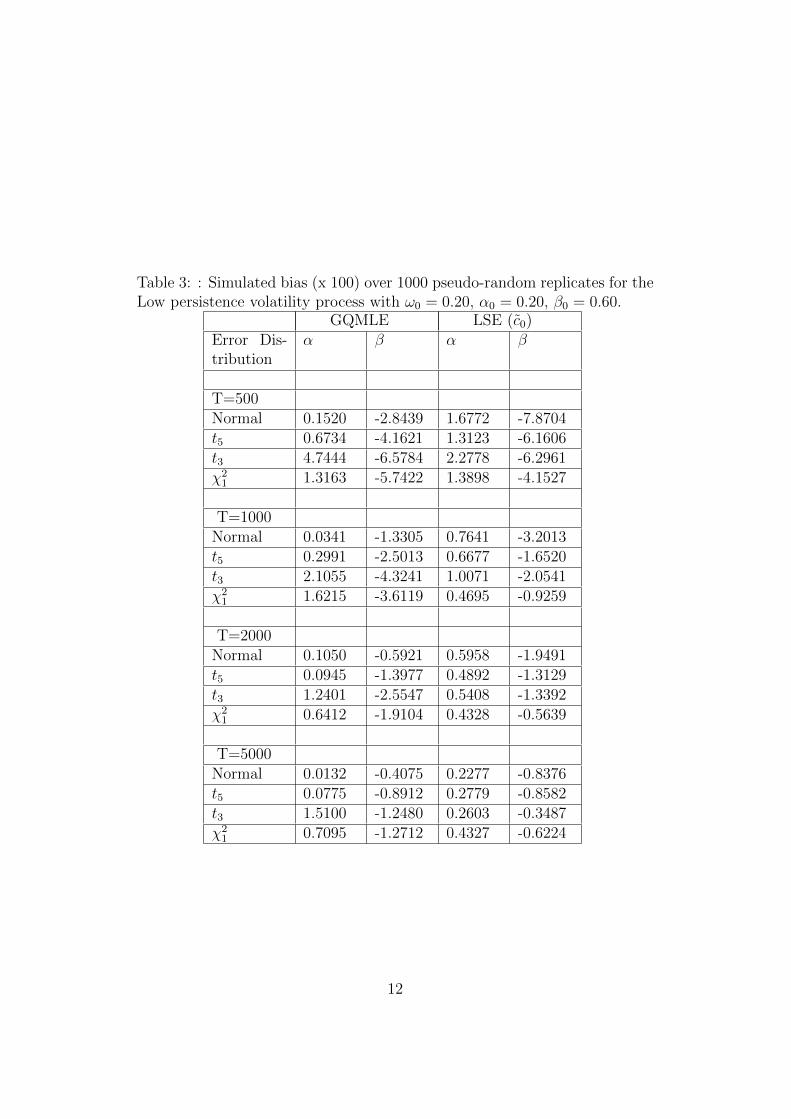
Table 3: : Simulated bias (x 100) over 1000 pseudo-random replicates for theLow persistence volatility process with ω0 = 0.20, α0 = 0.20, β0 = 0.60.

GQMLE LSE (c0)Error Dis-tribution

α β α β

T=500Normal 0.1520 -2.8439 1.6772 -7.8704t5 0.6734 -4.1621 1.3123 -6.1606t3 4.7444 -6.5784 2.2778 -6.2961χ2

1 1.3163 -5.7422 1.3898 -4.1527

T=1000Normal 0.0341 -1.3305 0.7641 -3.2013t5 0.2991 -2.5013 0.6677 -1.6520t3 2.1055 -4.3241 1.0071 -2.0541χ2

1 1.6215 -3.6119 0.4695 -0.9259

T=2000Normal 0.1050 -0.5921 0.5958 -1.9491t5 0.0945 -1.3977 0.4892 -1.3129t3 1.2401 -2.5547 0.5408 -1.3392χ2

1 0.6412 -1.9104 0.4328 -0.5639

T=5000Normal 0.0132 -0.4075 0.2277 -0.8376t5 0.0775 -0.8912 0.2779 -0.8582t3 1.5100 -1.2480 0.2603 -0.3487χ2

1 0.7095 -1.2712 0.4327 -0.6224

12

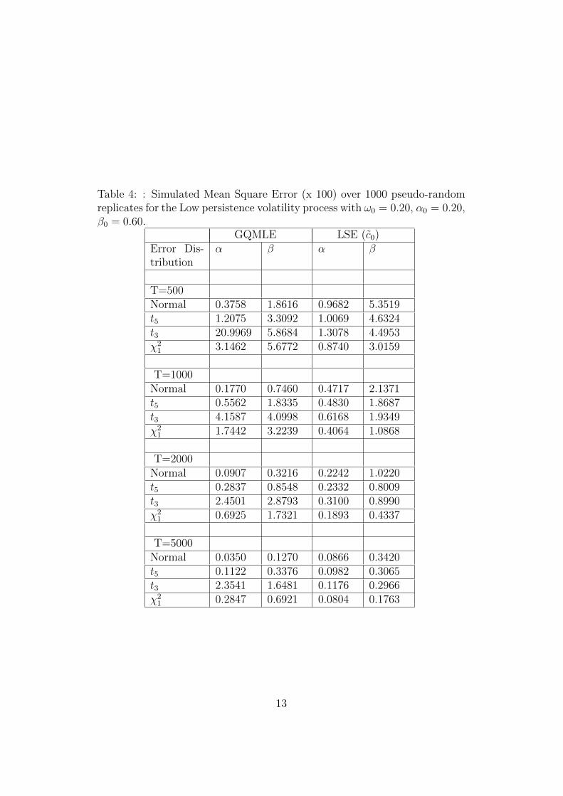
Table 4: : Simulated Mean Square Error (x 100) over 1000 pseudo-randomreplicates for the Low persistence volatility process with ω0 = 0.20, α0 = 0.20,β0 = 0.60.

GQMLE LSE (c0)Error Dis-tribution

α β α β

T=500Normal 0.3758 1.8616 0.9682 5.3519t5 1.2075 3.3092 1.0069 4.6324t3 20.9969 5.8684 1.3078 4.4953χ2

1 3.1462 5.6772 0.8740 3.0159

T=1000Normal 0.1770 0.7460 0.4717 2.1371t5 0.5562 1.8335 0.4830 1.8687t3 4.1587 4.0998 0.6168 1.9349χ2

1 1.7442 3.2239 0.4064 1.0868

T=2000Normal 0.0907 0.3216 0.2242 1.0220t5 0.2837 0.8548 0.2332 0.8009t3 2.4501 2.8793 0.3100 0.8990χ2

1 0.6925 1.7321 0.1893 0.4337

T=5000Normal 0.0350 0.1270 0.0866 0.3420t5 0.1122 0.3376 0.0982 0.3065t3 2.3541 1.6481 0.1176 0.2966χ2

1 0.2847 0.6921 0.0804 0.1763

13

Table 5: : Simulated bias (x 100) over 1000 pseudo-random replicates for theMedium persistence volatility process with ω0 = 0.10,α0 = 0.10, β0 = 0.80.

GQMLE LSE (c0)Error Dis-tribution

α β α β

T=500Normal 0.0819 -4.3154 2.0268 -18.9382t5 0.9619 -6.2946 2.2417 -14.2595t3 4.0729 -11.2138 2.5491 -13.5762χ2

1 2.4365 -9.4596 1.5899 -7.5517

T=1000Normal 0.0669 -1.8689 1.2244 -10.0284t5 0.4380 -3.1592 1.1640 -7.0427t3 1.6529 -6.5714 1.2531 -5.2478χ2

1 1.1753 -4.5431 0.6193 -2.4494

T=2000Normal 0.0489 -0.9953 0.7294 -3.3948t5 0.3451 -1.6849 0.5889 -2.0423t3 2.2618 -2.9461 0.5049 -1.7278χ2

1 0.7206 -2.3926 0.1515 -0.6626

T=5000Normal 0.0058 -0.3597 0.3141 -1.2743t5 0.1450 -0.6466 0.2254 -0.8282t3 1.4510 -2.0021 0.2324 -0.5920χ2

1 0.2104 -0.7452 0.1319 -0.3485

14

Table 6: : Simulated Mean Square Error (x 100) over 1000 pseudo-randomreplicates for the Medium persistence volatility process with ω0 = 0.10,α0 =0.10, β0 = 0.80.

GQMLE LSE (c0)Error Dis-tribution

α β α β

T=500Normal 0.2022 1.8818 0.5225 11.4787t5 0.5860 2.8612 0.5130 7.9819t3 7.4474 5.5943 0.7750 7.9700χ2

1 1.9106 4.8282 0.3737 4.1705

T=1000Normal 0.0814 0.6311 0.2662 5.4332t5 0.3151 1.3267 0.2441 3.6226t3 1.8726 2.9159 0.2570 2.5763χ2

1 0.5817 2.1179 0.1246 1.0478

T=2000Normal 0.0393 0.2548 0.1130 1.3540t5 0.1139 0.5641 0.1061 0.8534t3 2.6353 1.6702 0.1128 0.6794χ2

1 0.2732 0.9862 0.0564 0.2240

T=5000Normal 0.0163 0.0831 0.0419 0.2913t5 0.0477 0.1737 0.0353 0.1521t3 1.0281 0.9039 0.0410 0.1307χ2

1 0.0844 0.2784 0.0213 0.0707

15

Table 7: : Simulated bias (x 100) over 1000 pseudo-random replicates for theHigh persistence volatility process with ω0 = 0.01,α0 = 0.09, β0 = 0.90.

GQMLE LSE (c0)Error Dis-tribution

α β α β

T=500Normal 0.9561 -2.3596 1.1684 -8.7027t5 2.6349 -4.3835 1.5388 -5.8657t3 5.9734 -7.9647 2.0560 -7.3836χ2

1 5.1557 -7.4965 1.3561 -3.6250

T=1000Normal 1.3435 -1.8156 0.5509 -2.1848t5 2.4439 -2.7361 0.6940 -1.7094t3 4.4315 -4.8574 0.6724 -1.8669χ2

1 5.3084 -3.6914 0.4448 -0.7459

T=2000Normal 1.4091 -1.3727 0.2109 -0.5496t5 2.0595 -1.6655 0.1693 -0.4252t3 3.1710 -3.0927 0.2558 -0.4894χ2

1 3.7968 -2.6326 0.2052 -0.2945

T=5000Normal 1.6350 -1.5051 0.1300 -0.2902t5 1.9663 -1.2381 0.0633 -0.1555t3 2.9075 -2.0648 0.1768 -0.2310χ2

1 2.4037 -1.0823 0.1242 -0.1656

16

Table 8: : Simulated Mean Square Error (x 100) over 1000 pseudo-randomreplicates for the High persistence volatility process with ω0 = 0.01,α0 = 0.09,β0 = 0.90.

GQMLE LSE (c0)Error Dis-tribution

α β α β

T=500Normal 0.4972 0.4333 0.2831 5.2575t5 1.0339 0.9597 0.3238 2.9953t3 18.5386 2.8339 0.5464 4.1824χ2

1 4.2910 2.4702 0.2873 1.8381

T=1000Normal 0.3060 0.1981 0.1177 0.7986t5 0.7952 0.4527 0.1193 0.5341t3 10.1927 1.4221 0.1322 0.6742χ2

1 9.7875 0.7489 0.0708 0.1113

T=2000Normal 0.2468 0.1437 0.0504 0.0639t5 0.6320 0.2137 0.0418 0.0453t3 2.7973 0.5827 0.0487 0.1306χ2

1 3.4428 0.6729 0.0263 0.0240

T=5000Normal 0.2346 0.1520 0.0167 0.0203t5 0.9340 0.2495 0.0150 0.0156t3 2.5498 0.5194 0.0193 0.0180χ2

1 9.7692 0.2160 0.0103 0.0096

17

Figure 1: S&P 500 daily returns from 5.01.1971 to 30.05.2006.

18

Figure 2: 30 minutes returns on the USD/CHF exchange rate from 1.04.1996to 30.03.2001.

19

proxy of volatility and then refer to the following well-known loss functions:the Mean Square Error (MSE), the QLIKE, the Mean Absolute Error (MAE)and its equivalent formulation in terms of standard deviations (MAE-SD).A discussion of these loss functions and their properties can be found inPatton (2011). For MSE and QLIKE, the expected loss is minimized ifthe volatility estimate used to compute the loss function coincides with thetrue conditional variance. Differently, for MAE and MAE-SD, optimality isachieved in correspondence of the true conditional median of the squaredreturns.

The volatility of each of the two series, S&P 500 and USD/CHF exchangerate returns, has been modelled as a GARCH(1,1) whose parameters havebeen estimated by QML and by the LSE (Table 9). For the S&P 500, theestimates of the ARCH coefficient α obtained by the LSE are substantiallylower than that yielded by the GQMLE while the opposite applies to theGARCH parameterβ. Furthermore, it is interesting to analyze the behaviourof the different estimators under the four loss functions considered (Table 8).For the MSE, all the estimators yield very similar performances. The onlyexception is given by the LSE constructed under the assumption of Cauchyerrors which is characterized by a value of the MSE much higher than wasobserved for its competitors.

A different picture arises if we consider the QLIKE criterion. For thedaily S&P 500 returns series, except for the Cauchy case, the performance ofLSE is quite close to that of the GQMLE. The gap substantially increases inthe case of the 30 minutes USD/CHF exchange rate returns. For the othertwo loss functions considered, MAE and MAE-SD, and for both datasets, theLSE is always outperforming the QMLE. The LSE performance is optimizedif we estimate the scaling constant c0 under the assumption of Cauchy errorswith location and scale parameters equal to 0 and 1, respectively. However,in general, it is worth noting that the performance of the LSE appears to bequite robust to the choice of the scaling factor c0.

The message we get from these results is that, if one is interested in theconditional variance of returns as a measure of volatility, no clear advantagederives from using the LSE instead of the usual GQMLE. Differently, if thefocus is on an alternative measure of volatility, such as the conditional medianof squared returns, the use of the LSE can potentially allow for substantialaccuracy gains.

Finally, in order to evaluate the ability of the different estimators tocorrectly reproduce volatility persistence, we have compared the sample au-tocorrelation of squared returns with the autocorrelation function impliedby each of the estimated models (Figure 1 and Figure 2). For this exer-cise, however, we haven’t considered the LSE obtained under the assumption

20

Table 9: GARCH(1,1) parameter estimates under different estimators (* x10−4). Key to table: LS-D is the Least Squares estimator under distributionD (N=Normal, C=Cauchy, t5= Student’s with 5 df.)

S&P 500 USD/CHFω α β ω α β

QML 0.0007* 0.0658 0.9271 0.0448 0.0832 0.8752LS-N 0.0036 0.0395 0.9486 0.0615* 0.1293 0.8302LS-t5 0.0030 0.0322 0.9478 0.0499* 0.1030 0.8312LS-C 0.0013 0.0131 0.9386 0.0208* 0.0374 0.8259

Table 10: Evaluation of volatility estimates for the daily S&P 500 and 30min. USD/CHF returns by means of different loss functions: MAE, MSEand MSE-LOG. Key to table: LS-D is the Least Squares estimator underdistribution D (N=Normal, C=Cauchy, t5= Student’s with 5 df.)

S&P 500 USD/CHFMSE QLIKE MAE MAE-

SD

MSE QLIKE MAE MAE-

SD

QML 34.63 0.72 1.06 0.53 14.69 0.90 1.19 0.60LS-N 34.53 0.74 0.99 0.49 14.77 1.45 1.08 0.53LS-t5 34.56 0.82 0.93 0.46 14.76 1.73 1.02 0.50LS-C 35.41 2.60 0.89 0.44 15.58 5.50 0.95 0.47

21

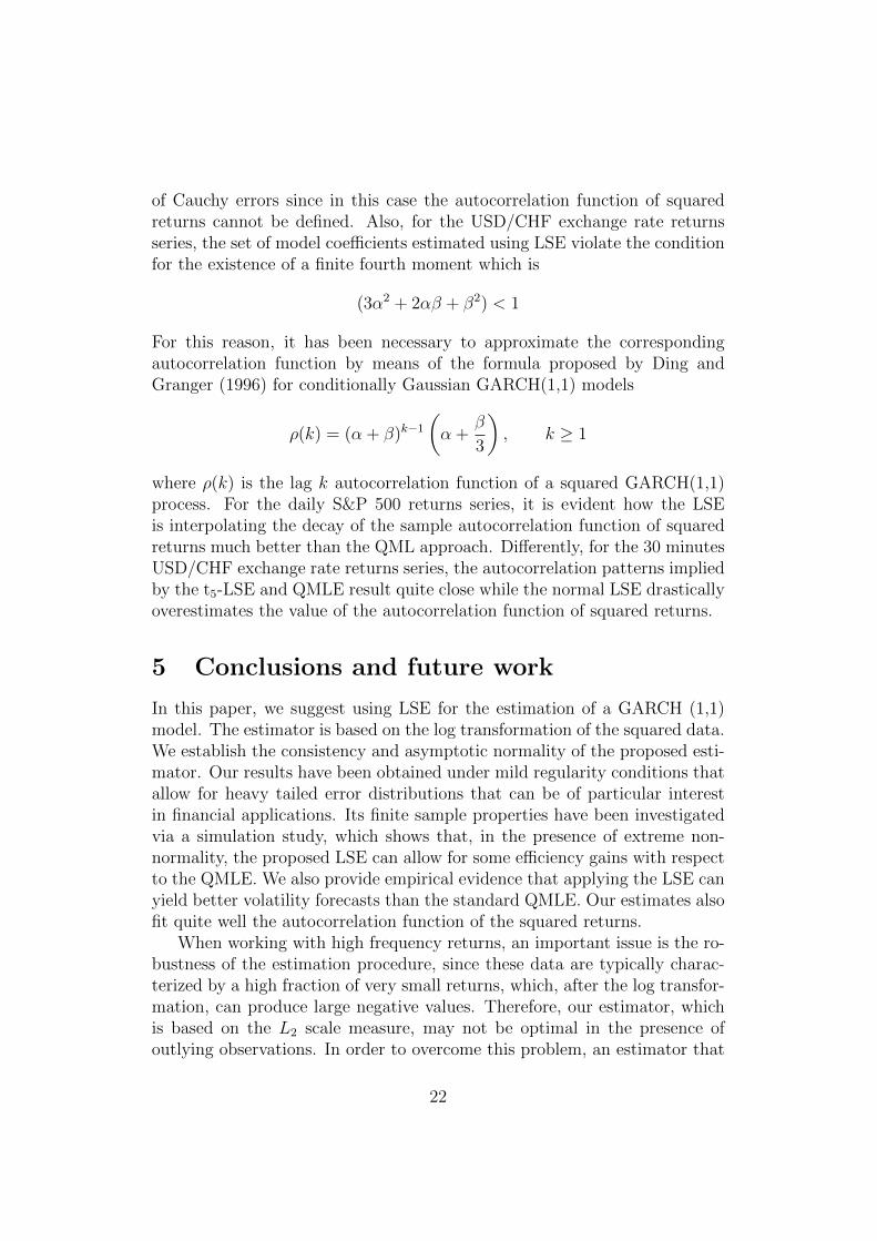
of Cauchy errors since in this case the autocorrelation function of squaredreturns cannot be defined. Also, for the USD/CHF exchange rate returnsseries, the set of model coefficients estimated using LSE violate the conditionfor the existence of a finite fourth moment which is

(3α2 + 2αβ + β2) < 1

For this reason, it has been necessary to approximate the correspondingautocorrelation function by means of the formula proposed by Ding andGranger (1996) for conditionally Gaussian GARCH(1,1) models

ρ(k) = (α + β)k−1

(α +

β

3

), k ≥ 1

where ρ(k) is the lag k autocorrelation function of a squared GARCH(1,1)process. For the daily S&P 500 returns series, it is evident how the LSEis interpolating the decay of the sample autocorrelation function of squaredreturns much better than the QML approach. Differently, for the 30 minutesUSD/CHF exchange rate returns series, the autocorrelation patterns impliedby the t5-LSE and QMLE result quite close while the normal LSE drasticallyoverestimates the value of the autocorrelation function of squared returns.

5 Conclusions and future work

In this paper, we suggest using LSE for the estimation of a GARCH (1,1)model. The estimator is based on the log transformation of the squared data.We establish the consistency and asymptotic normality of the proposed esti-mator. Our results have been obtained under mild regularity conditions thatallow for heavy tailed error distributions that can be of particular interestin financial applications. Its finite sample properties have been investigatedvia a simulation study, which shows that, in the presence of extreme non-normality, the proposed LSE can allow for some efficiency gains with respectto the QMLE. We also provide empirical evidence that applying the LSE canyield better volatility forecasts than the standard QMLE. Our estimates alsofit quite well the autocorrelation function of the squared returns.

When working with high frequency returns, an important issue is the ro-bustness of the estimation procedure, since these data are typically charac-terized by a high fraction of very small returns, which, after the log transfor-mation, can produce large negative values. Therefore, our estimator, whichis based on the L2 scale measure, may not be optimal in the presence ofoutlying observations. In order to overcome this problem, an estimator that

22

Figure 3: Implied autocorrelation function of squared returns versus sampleautocorrelations for the S&P500 series (lags from 1 to 100) : QML andalternative LSE.

23

Figure 4: Implied autocorrelation function of squared returns versus sampleautocorrelations for the USD/CHF series (lags from 1 to 100) : QML andalternative LSE.

24

employs a more robust scale measure such as the S-estimator can be used.In addition, our results can be extended to the GARCH (p,q) case as well asto other GARCH “type” models. The investigation of these issues is left forfuture work.

25

Appendix

Throughout the Appendix, K will denote a generic positive number that mayvary in different uses. To simplify the notation we set

hit(θ) =∂ht(θ)

∂θi, hijt(θ) =

∂ht(θ)

∂θi∂θj, ˙hit(θ) =

∂ht(θ)

∂θi, ¨hijt(θ) =

∂ht(θ)

∂θi∂θj

Let ∇`t(θ) = ∂`t(θ)∂θ

, ∇`it(θ) = ∂`t(θ)∂θi

and ∇2`t(θ) = ∂`t(θ)∂θ∂θ′

, ∇2`ijt(θ) = ∂`t(θ)∂θi∂θj

denote the first and second derivatives of `t(θ) (and their elements), respec-tively.

5.1 A. Proofs of theorems

Proof of Theorem 1:

We use similar arguments as in Theorem 5.3.1 of Straumann (2005, p.101)showing strong consistency by contradiction. Suppose that θn 6→θ0 a.s. so forsome arbitrary γ > 0, the compact set F = ω ∈ Ω| lim supn→∞ ||θn− θ0|| ≥γ, θn ∈ Θ has a positive probability. Since the set N = Θ∩θ : |θn−θ0| ≥γ is compact, there exists a non-null subset F ⊂ F such that for everyω ∈ F ,one can find inN, a convergent subsequenceθni

(ω)→ θ ∈ N. By definition ofthe LSE

lim infn→∞

1ni

∑ni

t=1˜t(θ0) ≥ lim inf

n→∞infθ∈N

1ni

∑ni

t=1˜t(θ)

= lim infn→∞

1ni

∑ni

t=1˜t(θni

)

From Lemma 5,

lim infn→∞

1ni

∑ni

t=1 `t(θ0) ≥ lim infn→∞1ni

∑ni

t=1 `t(θni) (11)

The inequality above and Lemmas 4(ii)-(iii) imply that with positive prob-ability E`t(θ0) ≥ E infθ∈N `t(θ). This result contradicts Lemma 4(i) whichstates that in the limit Qn(θ) is uniquely minimized at θ0. Since γ > 0 isarbitrary, the strong consistency follows.

Proof of Theorem 2: By Theorem 1, θn → θ0 a.s. so for n sufficientlylarge θn ∈ Θ0 a.s. and the results of Lemmas 6-7 can be applied. Using a

26

mean-value expansion of Qn(θn) =∑n

t=1˜t(θn) around θ0, we have

0 = n−0.5∑n

t=1∇˜

t(θn) (12)

= n−0.5∑n

t=1∇˜

t(θ0) +(

1n

∑nt=1∇2 ˜

t(θn))√

n(θn − θ0)

= n−0.5∑n

t=1∇˜

t(θ0)

+[(

1n

∑nt=1∇2 ˜

t(θn)− 1n

∑nt=1∇2`t(θn)

)+(

1n

∑nt=1∇2`t(θn) + J

)− J

]√n(θn − θ0)

where θn lies on the chord between θn and θ0.Lemma 6 and the asymptotic equivalence lemma (e.g. see White (1994),

p.172) imply that 1√n

∑nt=1 ∂

˜t(θ0)

/∂θ →

DN(0, H) where H = κJ and J is a

positive definite matrix. Next, Lemmas 7(i)-(ii) imply that the first and sec-ond terms, inside the square brackets in (12), converge a.s. to zero. Hence,to complete the proof it suffices to solve (12) and apply Slutsky’s theorem.

Proof of Theorem 3: The result follows immediately from Theorems 1-2and Lemma 7.

B. Lemmata

Lemma 1: Under Assumptions A1-A4, for some p ∈ (0, 1)

i) (y2t , h0t) are strictly stationary and ergodic and E (hp0t) <∞, E (|yt|2p) <∞

ii)infθ∈Θ `t(θ), `t(θ), ∇`it(θ) and∇2`ijt(θ) are strictly stationary and ergodic.

iii) E (η2t ) <∞

Proof :

i) Under Assumption A2, the result follows directly from (1)-(2) and Theo-rem 4 of Nelson (1990).

ii) From (7)-(8) and Theorem 2.7 of Stinchcombe and White (1992), we havethat infθ∈Θ `t(θ) is measurable functions of yt−j for all j ≥ 0, and thus are

27

strictly stationary and ergodic (see Stout (1974), Theorem 3.5.8). The sameresult follows for `t(θ) and its derivatives by Lemma 2(ii) of Lee and Hansen(1994).

iii) Let w = ε2t , F (x) = Pr(w ≤ x) and f(x) be the density function, since

ηt = w − c0, the result follows if∫ +∞

0[ln(w)]2f(w)dw <∞. By integration

by parts

1∫0

[ln(w)]2f(w)dw = [ln(1)]2F (1)−1∫r

ln(w)

wF (w)dw −

r∫0

ln(w)

wF (w)dw

The first integral on the RHS is bounded for any r > 0. Hence, by Assump-tion A4, when r > 0 is small enough, there exists some δ > 0 such that thesecond integral is bounded by K

∫ r

0wδ ln(w)dw. This integral is finite for any

δ > 0. For w ≥ 1 we get∫ +∞

1[ln(w)]2f(w)dw <

∫ +∞1

w2sf(w)dw ≤ E|εt|2s,since ln(w) < ws/2 for any s > 0, and the desired result follows by Assump-tion A3.

Lemma 2: Under Assumptions A1-A4, for some p ∈ (0, 1)

i) E(

supθ∈Θ

∣∣∣ht(θ)− ht(θ)∣∣∣p) = O(βt) and E| supθ∈Θ ht(θ)|p < ∞.

ii) E(

supθ∈Θ0

∣∣∣hit(θ)− ˙hit(θ)∣∣∣p) = O(βt) for all i.

iii) E(

supθ∈Θ0

∣∣∣hijt(θ)− ¨hijt(θ)∣∣∣p) = O(βt) for all i, j.

Proof : i) By iterating (7) and using the fact α0y2t−1−i ≤ h0t, we get

ht(θ) = ω + αy2t−1 + βht−1(θ) (13)

=∑t−1

i=0(ω + αy2

t−1−i)βi + βth1(θ)

=∑∞

i=0(ω + αy2

t−1−i)βi

=ω

1− β+ α

∑∞

i=0βiy2

t−1−i

≤ ω

1− β+

α

α0

∑∞

i=0βih0t

28

Hence, the cr inequality ((a + b)q ≤ aq + bq for all a, b > 0, q ∈ [0, 1]) andLemma 1(i) imply that for some p ∈ (0, 1),

E| supθ∈Θ

ht(θ)|p ≤ K +KEhp0t < ∞ (14)

Now, without loss of generality, set h1 = 0.5(ω + ω), by iterating (5) weobtain

ht(θ) = ω + αy2t−1 + βht−1(θ) =

∑t−1

i=0(ω + αy2

t−1−i)βi + βth1 (15)

Henceht(θ)− ht(θ) = ω + αy2

t−1 + βht−1(θ) = βt(h1 − h1(θ)) (16)

and by (16),

E supθ∈Θ0

∣∣∣ht(θ)− ht(θ)∣∣∣p ≤ βt(hp1 + E supθ∈Θ0

|h1(θ)|p) ≤ Kβt (17)

Further, by Lemma 1(i) and the cr inequality

E(ω + αy2t−1−i)

p <∞ (18)

and

E

(supθ∈Θ

∣∣∣ht(θ)∣∣∣p) ≤∑t−1

i=0E(ω + αy2

t−1−i)pβip + βpthp1 <∞

ii) We start by showing that for some p ∈ (0, 1) and all i,

E

(supθ∈Θ0

∣∣∣hit(θ)∣∣∣p) <∞ (19)

By (13) and the fact that y2t−1−i ≤ α−1

0 h0t,

∂ht(θ)

∂ω≤ 1

1− β(20)

∂ht(θ)

∂α=

∑∞

i=0βiy2

t−1−i ≤1

α

[∑∞

i=0αβiy2

t−1−i

]≤ 1

αht(θ) (21)

∂ht(θ)

∂β=

∑∞

i=1iβi(ω + αy2

t−1−i) (22)

≤∑∞

i=1iβi(ω +

α

α0

h0t

)≤ ω

∑∞

i=1iβi +

α

α0

∑∞

i=0βih0t

29

The term in (20) is bounded and admits moments of any order. As for(21)-(22), the result follows directly from the cr inequality and Lemma 1(i).In view of (16), almost surely,

supθ∈Θ0

∣∣∣hit(θ)− ˙hit(θ)∣∣∣ ≤ tβ(t−1)(h1 + sup

θ∈Θ0

h1(θ)) + βt supθ∈Θ0

|hi1(θ)| ≤ Kβt

the desired result follows by (14), (19) and the cr inequality.

iii) From (20)-(22) and direct calculations we get,

∂2ht∂ω2

=∂2ht∂α2

=∂2ht∂ω∂α

= 0,∂2ht∂ω∂β

1

β≤∑∞

i=1iβi (23)

which are bounded and admit moments of any order. We also find

∂2ht∂α∂β

≤ α∑∞

i=1iβiy2

t−1−i ≤α

α0

∑∞

i=1iβih0t (24)

∂2ht∂β2

=1

β

∑∞

i=2i(i− 1)(ω + αy2

t−1−i)βi (25)

So, similar to Lemma 2(ii) we can show that for some 0 < p < 1,

E

(supθ∈Θ0

∣∣∣hijt(θ)∣∣∣p) <∞ (26)

for all i, j. In view of (16), almost surely,

supθ∈Θ0

∣∣∣hijt(θ)− ¨hijt(θ)∣∣∣ ≤ t(t− 1)β(t−2)[h1 + sup

θ∈Θ0

h1(θ)]

+ tβ(t−1) supθ∈Θ0

|hj1(θ)|+ tβt−1 supθ∈Θ0

|hi1(θ)|

+ βt supθ∈Θ0

|hij1(θ)|

and by (14), (19), (26) and the cr inequality the desired result follows.

Lemma 37: Under Assumptions A1-A4, for all r ≥ 1

7Note that this lemma extends Lemma 4 of Lumsdaine (1996) and Lemmas 8 and 10 ofLee and Hansen (1994), since our results apply to moments of any order.

30

i)∥∥∥supθ∈Θ0 h−1

t (θ)hit(θ)∥∥∥r<∞ for all i

ii)∥∥∥supθ∈Θ0 h−1

t (θ)hijt(θ)∥∥∥r<∞ for all i, j

iii)∥∥∥supθ∈Θ0 h−1

t (θ) ˙hit(θ)∥∥∥r< ∞ for all i, and

∥∥∥supθ∈Θ0 h−1t (θ)¨hijt(θ)

∥∥∥r< ∞

for all i, j.

Proof : i) Eq. (20) and (21) imply that the derivative of ht with respectto ω and α (divided by ht) are bounded and hence admits moments of anyorder. However, this is not true for the derivative with respect to β. From(13) we get ht(θ) ≥ ω + (ω + αy2

t−1−i)βi for all i ≥ 1. Using the fact that

x/(1+x) < xp/r for all x ≥ 0 and any p ∈ (0, 1),r ≥ 1 (this idea of exploitingthis inequality is due to Boussama (2000)), we get

∂ht∂β

1

ht≤ 1

β

∑∞

i=1i

(ω + αy2t−1−i)β

i

ω + (ω + αy2t−1−i)β

i(27)

≤ 1

β

∑∞

i=1i

[(ω + αy2

t−1−i)βi

ω

]p/r≤ 1

βωp/r

∑∞

i=1iβip/r(ω + αy2

t−1−i)p/r

Therefore, by (18) and Minkowski’s inequality we get∥∥∥∥ supθ∈Θ0

∂ht∂β

1

ht

∥∥∥∥r

≤ K∑∞

i=1iβi[E(ω + αy2

t−1−i)p]1/r

<∞

ii) From (23)-(25), we observe that the relevant second derivatives satisfy

∂2ht∂β2

1

ht≤ 1

β

∑∞

i=2i(i− 1)

(ω + αy2t−1−i)β

i

ω + (ω + αy2t−1−i)β

i(28)

and∂2ht∂α∂β

≤∑∞

i=1iβi

(ω + αy2t−1−i)

ω + (ω + αy2t−1−i)β

i,

(the other derivatives are naturally bounded). Using the same arguments asin part (i) of the lemma the desired results follow.

iii) The proof is similar to part (i)-(ii) of the lemma, hence omitted.

31

Lemma 4: Under Assumptions A1-A5,

i) E(`t(θ0)) ≤ E(`t(θ)) with equality if and only if θ 6= θ0.

ii) For any compact set N ⊆ Θ,

lim infn→∞

infθ∈N

1n

∑nt=1 `t(θ) ≥ E infθ∈N `t(θ).

iii) limn→∞1n

∑nt=1 `t(θ0) = E`t(θ0).

iv) E(|supθ∈Θ lnht(θ)|2

)<∞ and E(z2

t ) <∞

Proof :

i) Note that

E(`t(θ))− E(`t(θ0)) = 12E [(zt − lnht(θ))

2 − η2t ] (29)

= 12E [ln(h0t − ln(ht(θ))]

2 + E [ln(h0t/ht)] E(ηt)

= 12E [ln (ht(θ0)/ht(θ))]

2 ≥ 0

with equality if and only if ht(θ0) = ht(θ)a.s.

ii) For any compact set N ⊆ Θ we have,

lim infn→∞

infθ∈N

1n

n∑t=1

`t(θ) ≥ lim infn→∞1n

n∑t=1

infθ∈N `t(θ) (30)

Further, note E`t(θ) <∞ is well defined and belongs to < ∪ +∞. Hence,by Lemma 1(ii), we can apply the ergodic theorem (see Billingsley (1995)p.284) to the stationary and ergodic sequence infθ∈N `t(θ)t to obtain

lim infn→∞

infθ∈N

1n

∑nt=1 `t(θ) ≥ lim inf

n→∞1n

∑nt=1 infθ∈N `t(θ) (31)

≥ E

(infθ∈N

`t(θ)

)iii) Note that E`t(θ0) = E(η2

t ) < ∞ by Lemma 1(iii). The desired resultfollows from Lemma 1(ii), and the ergodic theorem.

32

iv) Notice, that since 0 < ω ≤ ht(θ) for any p > 0,

ln(ω) ≤∣∣∣∣supθ∈Θ

lnht(θ)

∣∣∣∣ ≤ K +

∣∣∣∣supθ∈Θ

ht(θ)

∣∣∣∣p/2By (14) we obtain that E

(|supθ∈Θ lnht(θ)|2

)< ∞. This result and Lemma

1(iii) also imply that E(z2t ) is finite.

Lemma 5: Under Assumptions A1-A4,

supθ∈Θ

∣∣∣ 1n

∑nt=1

(˜t(θ)− `t(θ)

)∣∣∣ →a.s.

0

Proof :Let At(θ) = ˜

t(θ) − `t(θ). To prove this result, it suffices to check thatE supθ∈Θ |At(θ)|q, is bounded by a summable sequence in t, for some q ≥ 0.Indeed then (by Markov inequality) for all λ > 0,∑∞

t=1P(sup

θ∈Θ|At(θ)| > λ) ≤

∑∞

t=1E supθ∈Θ|At(θ)|q/λq <∞ (32)

so that the Borel-Cantelli lemma implies that supθ∈Θ |At(θ)| converges tozero a.s. This convergence and the Cesaro lemma imply the desired result.

Now, since ht, ht ≥ ω > 0, an application of the mean-value theoremlead to

| ln ht(θ)− lnht(θ)| ≤ K|ht(θ)− ht(θ)| (33)

So, from (4), (8) and the cr inequality, for some p ∈ (0, 1)

E supθ∈Θ|˜t(θ)− `t(θ)|p/4 ≤ E sup

θ∈Θ

[∣∣∣ln ht(θ)− lnht(θ)∣∣∣p/4

×∣∣∣ln ht(θ)− lnht(θ) + 2 (zt + lnht(θ))

∣∣∣p/4]

≤ E

[supθ∈Θ

∣∣∣ht(θ)− ht(θ)∣∣∣p/2 ∣∣∣∣1 + zt + supθ∈Θ

lnht(θ)

∣∣∣∣p/4]

≤ KE

(supθ∈Θ

∣∣∣ht(θ)− ht(θ)∣∣∣p) = O(βt)

The second inequality holds by (33). The third inequality holds by the crand Cauchy-Schwarz inequalities and Lemma 4(iv). The last equality holds

33

by Lemma 2(i).

Lemma 6: Under Assumptions A1-A5,

i)∣∣∣n−1/2

∑nt=1

(∇˜

t(θ0)−∇`t(θ0))∣∣∣ → 0 a.s.

ii) n−1/2∑n

t=1∇`t(θ0)→DN (0, κJ) where J is positive definite and κ = E(η2

t ).

Proof :

i) We use the proof idea of Lemma 8 in Robinson and Zaffaroni (2006). Let.Bt = ∇`it(θ0)−∇˜

it(θ0), the gradients of (4) and (8) are given by

∇˜it(θ0) = (zt − ln h0t)

˙h0it

h0t

, ∇`it(θ0) = (zt − lnh0t)h0it

h0t

= ηth0it

h0t

(34)

where h0it = hit(θ0), ˙h0it = ˙hijt(θ0). Hence,

Bt = ∇`it(θ0)−∇˜it(θ0) = ηt

(h0it

h0t

−˙h0it

h0t

)+

˙h0it

h0t

ln

(h0t

h0t

)and

n−1/2∑n

t=1Bt ≤ n−1/2K

∑n

t=1ηt

(h0it − ˙h0it

)+

˙h0it

h0t

(h0it − h0it

)(35)

Next, by application of the cr and Cauchy-Schwarz inequalities, we get that∑∞t=1 |Bt| has some finite p > 0 moment and thus by Loeve (p. 121) is a.s.

finite. Further Lemma 2(i)-(ii) implies that a.s. |Bt| ≤ Kβt, ∀t. Hence, byKronecker lemma (35) tends to zero a.s. as n → ∞ and the desired resultfollows

ii) From (34)

E (∇`it(θ0)|Ft−1) =h0it

h0t

E (ηt|Ft−1) =h0it

h0t

E (ηt) = 0

where Ft = σ(yt, yt−1, . . .) and

‖∇`it(θ0)∇`jt(θ0)‖ ≤ E(η2t

) ∥∥∥∥∥ h0it

h0t

∥∥∥∥∥2

∥∥∥∥∥ h0jt

h0t

∥∥∥∥∥2

<∞

34

by applying the Cauchy-Schwarz inequality and Lemmas 1(iii) and 3(i).Thus, we have shown that the second moment of each element of the gradientis finite hence E |∇`t(θ0)∇`t(θ0)′| <∞. These results and Lemma 1(ii) implythat∇`t(θ0),Ft is a stationary, ergodic and martingale difference sequencewith finite variance

var(∇`t(θ0)) = E(η2t )E

(1

h20t

∂h0t

∂θ

∂h0t

∂θ′

)= κJ

Next, by using similar arguments used in Lemma 5 in Lumsdaine (1996) wecan show that J is a positive definite matrix. Thus, Theorem 23.1 of Billings-ley (1968) and the Cramer-Wold device imply that n−1/2

∑nt=1∇2`t(θ0) →

D

N(0, κJ).

Lemma 7: Under Assumptions A1-A5,

i) supθ∈Θ0

∣∣∣ 1n

∑nt=1

(∇2 ˜

t(θ)−∇2`t(θ))∣∣∣ → 0 a.s.

ii) If θn →a.s.

θ0, 1n

∑nt=1∇2`t(θn) →

a.s.−J

Proof :

i) First, let Ct(θ) = ∇2`ijt(θ) − ∇2 ˜ijt(θ). Using similar arguments as

in Lemma 5, it suffices to check that E supθ∈Θ0 |Ct(θ)|q is bounded by asummable sequence in t, for some q ≥ 0. Second, given (4) and (8) thesecond derivatives are

∇2 ˜ijt(θ) = (zt − ln ht)

¨hijt

ht− (zt − ln ht + 1)

˙hit˙hjt

h2t

(36)

and

∇2`ijt(θ) = (zt − lnht)hijtht− (zt − lnht + 1)

hithjth2t

(37)

Third, note

hit˙hjth2t

−˙hit

˙hjt

h2t

≤ K

hitht

[˙hit − hit

]+

˙hjt

ht

[˙hjt − hjt

](38)

35

Finally, using (36)-(38) we obtain

supθ∈Θ0

Ct(θ) ≤ supθ∈Θ0

(1 + ηt + ln

(h0t

ht

))(hijtht−

¨hijt

ht

)+hijt

htln

(htht

)

+

(hithjth2t

−˙hit

˙hjt

h2t

)+

˙hit˙hjt

h2t

ln

(htht

)

≤ K supθ∈Θ0

1 + ηt + ln

(h0t

ht

)(hijtht

+˙hit

ht

˙hjt

ht

)(ht − ht

)

+hitht

(˙hit − hit

)+

˙hjt

ht

(˙hjt − hjt

)+(hijt − ¨hijt

)

By applying Holder and Minkowski inequalities with Lemmas 2, 3 and 4(iv),we get for some q ∈ (0, 1) that E supθ∈Θ0 |Ct(θ)|q = O(βt) and the desiredresult follows.

ii) From (37), E (∇2`t(θ0)) = −J and

E supθ∈Θ0

∣∣∇2`ijt(θ)∣∣ ≤ E sup

θ∈Θ0

∣∣∣∣∣(

1 + ηt + ln

(h0t

ht

))(hijtht

+hithjth2t

)∣∣∣∣∣≤

1 + ||ηt||2 +

∥∥∥∥ supθ∈Θ0

ln

(h0t

ht

)∥∥∥∥2

∥∥∥∥∥ supθ∈Θ0

hijtht

∥∥∥∥∥2

+

∥∥∥∥∥ supθ∈Θ0

hitht

∥∥∥∥∥4

∥∥∥∥∥ supθ∈Θ0

hjtht

∥∥∥∥∥4

<∞

The second inequality holds by applying the Cauchy-Schwarz and Minkowskiinequalities. The last inequality holds by Lemma 1(iii), Lemmas 3 and 4(iv).From the ergodic theorem (see e.g., Billingsley (1995)),

supθ∈Θ0

∣∣ 1n

∑nt=1∇2`t(θ)− E (∇2`t(θ))

∣∣ →a.s.

0

Hence, given ε > 0∣∣∣ 1n

∑nt=1∇2`t(θn)− E

(∇2`t(θn)

)∣∣∣ < 12ε

36

a.s. for n sufficiently large. Since E (∇2`t(θ)) is continues∣∣∣E(∇2`ijt(θn))− E

(∇2`ijt(θ0)

)∣∣∣ < 12ε

a.s. for n sufficiently large since θn → θ0 a.s. and the desired result followsfrom an application of the triangle inequality, since ε is arbitrary.

37

References

[1] Andrews B. (2012). Rank based estimation for GARCH processes. Econo-metric Theory, 28(5), 1037-1064.

[2] Andrews D.W.K.(2001). Testing when a parameter is on the boundary ofthe maintained hypothesis. Econometrica, 69, 683-734.

[3] Berkes I. Horvath L. and P.S. Kokoszka (2003). GARCH processes: struc-ture and estimation. Bernoulli, 9, 201-227.

[4] Berkes I. and L. Horvath (2003). The rate of consistency of the quasi-maximum likelihood estimator. Statistics and Probability Letters, 61, 133-143.

[5] Billingsley P. (1968) Convergence of Probability Measures. New York,John Wiley.

[6] Billingsley P. (1995). Probability and Measure. New York, John Wiley.

[7] Bollerslev T. (1986). Generalized autoregressive conditional heteroskedas-ticity. Journal of Econometrics, 31, 307-327.

[8] Bollerslev T. and J.M. Wooldridge (1992). Quasi-maximum likelihood es-timation and inference in dynamic models with time-varying covariances.Econometric Reviews, 11, 143-172.

[9] Boussama F. (2000). Normalite asymptotique de l’estimateur du pesudo-maximum de vraisemblance d’un mode’le GARCH. C.R.Acad Sci. Paris,331, 81-84.

[10] Dacorogna M.M., Gencay R., Muller U., Olsen R.B. and O.V. Pictet(2001). An Introduction to High Frequency Finance. San Diego, CA: Aca-demic Press.

[11] Ding, Z. and C. W. J. Granger (1996). Modelling volatility persistenceof speculative returns: a new approach, Journal of Econometrics, 73,185–215.

[12] Francq C. and J-M. Zakoian (2007). Quasi-likelihood inference inGARCH processes when some coefficients are equal to zero. StochasticProcesses and their Applications, 117(9), 1265-1284.

38

[13] Francq C. and J-M. Zakoian (2009). A Tour in the asymptotic theory ofGARCH estimation, Handbook of Financial Time Series, 85-111, Berlin,Springer-Verlag.

[14] Francq C. and J-M. Zakoian (2013). Estimating the marginal law ofa time series with Applications to heavy-tailed distributions, Journal ofBusiness and Economic Statistics, 31(4), 412-425.

[15] Hall P. and Q. Yao (2003). Inference in ARCH and GARCH models withheavy-tailed errors. Econometrica, 71, 285-317.

[16] Hansen P.R and A.Lunde (2005). A forecast comparison of volatilitymodels: does anything beat a GARCH(1,1)? Journal of Applied Econo-metrics, 20(7), 873-889.

[17] Harvey A.C., Ruiz E. and N.G. Shephard (1994). Multivariate stochasticvariance models. Review of Economic Studies, 61, 247-264.

[18] Huang D., Wang H. and Q. Yao (2008). Estimating GARCH models:when to use what? Econometrics Journal, 11, pp. 27–38

[19] Lee S.W. and B.E. Hansen (1994). Asymptotic theory for theGARCH(1,1) quasi- maximum likelihood estimator. Econometric The-ory, 10, 29-52.

[20] Linton O, Pan J. and H Wang (2010). Estimation for A non-stationarysemi-strong GARCH(1,1) models with heavy-tailed errors. Econometrictheory, 26(1), 1-28.

[21] Loeve M. (1977). Probability Theory 1, New York, Springer.

[22] Lumsdaine, R.L. (1996). Consistency and asymptotic normality of thequasi-maximum likelihood estimator in IGARCH(1,1) and covariance sta-tionary GARCH (1,1) models. Econometrica, 64, 575-596.

[23] Mittnik S. and S.T. Rachev (2000) Stable Paretian Models in Finance.New York, John-Wiley.

[24] Nelson D.B. (1990). Stationarity and persistence in the GARCH(1,1)model. Econometric Theory, 6(3), 318-334.

[25] Mukherjee K. (2008). M-estimation in GARCH models. EconometricTheory, 24(6), 1530-1553.

39

[26] Patton A. (2011) Volatility forecast evaluation and comparison usingimperfect volatility proxies. Journal of Econometrics, 160, 246–256.

[27] Peng, L. and Q. Yao (2003). Least absolute deviation estimation forARCH and GARCH models. Biometrika, 90, 967-975.

[28] Rekkasa M. and A. Wong (2008). Implementing likelihood-based infer-ence for fat-tailed distributions. Finance Research Letters, 5(1), 32-46.

[29] Robinson P.M. and P. Zaffaroni (2006). Pseudo-maximum likelihood es-timation of ARCH(∞) models. Annals of Statistics, 34, 1049–1074.

[30] Ruiz E. (1994). Quasi-maximum likelihood estimation of stochasticvolatility models. Journal of Econometrics, 63, 289–306.

[31] Sakata S. and H. White (2001). S-estimation of nonlinear regres-sion models with dependent and heterogeneous observations. Journal ofEconometrics, 103, 5-72.

[32] Stinchcombe M. B. and H. White (1992). Some measurability resultsfor extrema of random functions over random sets. Review of EconomicStudies, 59 (3), 495-514.

[33] Straumann D. (2005) Estimation in Conditionally Heteroscedastic TimeSeries Models, Lecture Notes in Statistics, Springer.

[34] White H. (1994). Estimation, Inference and Specification Analysis. NewYork, Cambridge University Press.

40