252
MUSIC RECOMMENDATION AND DISCOVERY IN THE LONG TAIL ` Oscar Celma Herrada 2008
MUSIC RECOMMENDATION AND DISCOVERY
IN THE LONG TAIL
Oscar Celma Herrada
2008

c© Copyright by Oscar Celma Herrada 2008
All Rights Reserved
ii

To Alex and Claudia
who bring the whole endeavour into perspective.
iii

iv
Acknowledgements
I would like to thank my supervisor, Dr. Xavier Serra, for giving me the opportunity to
work on this very fascinating topic at the Music Technology Group (MTG). Also, I want to
thank Perfecto Herrera for providing support, countless suggestions, reading all my writings,
giving ideas, and devoting much time to me during this long journey.
This thesis would not exist if it weren’t for the the help and assistance of many people.
At the risk of unfair omission, I want to express my gratitude to them. I would like to thank
all the colleagues from MTG that were —directly or indirectly— involved in some bits of
this work. Special mention goes to Mohamed Sordo, Koppi, Pedro Cano, Martın Blech,
Emilia Gomez, Dmitry Bogdanov, Owen Meyers, Jens Grivolla, Cyril Laurier, Nicolas Wack,
Xavier Oliver, Vegar Sandvold, Jose Pedro Garcıa, Nicolas Falquet, David Garcıa, Miquel
Ramırez, and Otto Wust. Also, I thank the MTG/IUA Administration Staff (Cristina
Garrido, Joana Clotet and Salvador Gurrera), and the sysadmins (Guillem Serrate, Jordi
Funollet, Maarten de Boer, Ramon Loureiro, and Carlos Atance). They provided help,
hints and patience when I played around with the machines.
During my six months stage at the Center for Computing Research of the National Poly-
technic Institute (Mexico City) in 2007, I met a lot of interesting people ranging different
disciplines. I thank Alexander Gelbukh for inviting me to work in his research group, the
Natural Language Laboratory. Also, I would like to thank Grigori Sidorov, Tine Stalmans,
Obdulia Pichardo, Sulema Torres, and Yulema Ledeneva for making my stay so wonderful.
This thesis would be much more difficult to read —except for the “Spanglish” experts—
if it weren’t for the excellent work of the following people: Paul Lamere, Owen Meyers,
Terry Jones, Kurt Jacobson, Douglas Turnbull, Tom Slee, Kalevi Kilkki, Perfecto Herrera,
Alberto Lumbreras, Daniel McEnnis, Xavier Amatriain, and Neil Lathia. They not only
have helped me to improve the text, but have provided feedback, comments, suggestions,
and —of course— criticism.
v
Many people have influenced my research during these years. Furthermore, I have been
lucky enough to meet some of them. In this sense, I would like to acknowledge Elias
Pampalk, Paul Lamere, Justin Donaldson, Jeremy Pickens, Markus Schedl, Peter Knees,
and Stephan Baumann. I had very interesting discussions with them in several ISMIR (and
other) conferences. Other researchers whom I have learnt a lot, and I have worked with, are:
Massimiliano Zanin, Javier Buldu, Raphael Troncy, Michael Hausenblas, Roberto Garcıa,
and Yves Raimond.
I also want to thank some MTG veterans, whom I met and worked before starting the
PhD. They are: Alex Loscos, Jordi Bonada, Pedro Cano, Oscar Mayor, Jordi Janer, Lars
Fabig, Fabien Gouyon, and Enric Mieza. Also, special thanks goes to Esteban Maestre and
Pau Arumı for having such a great time while being PhD students.
Last but not least, this work would have never been possible without the encouragement
of my wife Claudia, who has provided me love and patience, and my lovely son Alex —who
altered my last.fm and youtube accounts with his favourite music. Nowadays, Cri–Cri, Elmo
and Barney, coexists with The Dogs d’Amour, Backyard Babies, and other rock bands. I
reckon that the two systems are a bit lost when trying to recommend me music and videos!.
Also, a special warm thanks goes to my parents Tere and Toni, my brother Marc and my
sister in law Marta, and the whole family in Barcelona and Mexico. At least, they will
understand what my work is about. . . hopefully.
This research was performed at the Music Technology Group of the Universitat Pompeu
Fabra in Barcelona, Spain. Primary support was provided by the EU projects FP6-507142
SIMAC1 and FP6-045035 PHAROS2, and by a Mexican grant from the Secretarıa de Rela-
ciones Exteriores (Ministry of Foreign Affairs) for a six months stage at the Center for
Computing Research of the National Polytechnic Institute (Mexico City).
1http://www.semanticaudio.org2http://www.pharos-audiovisual-search.eu/
vi
Abstract
Music consumption is biased towards a few popular artists. For instance, in 2007 only 1% of
all digital tracks accounted for 80% of all sales. Similarly, 1,000 albums accounted for 50%
of all album sales, and 80% of all albums sold were purchased less than 100 times. There is
a need to assist people to filter, discover, personalise and recommend from the huge amount
of music content available along the Long Tail.
Current music recommendation algorithms try to accurately predict what people de-
mand to listen to. However, quite often these algorithms tend to recommend popular —or
well–known to the user— music, decreasing the effectiveness of the recommendations. These
approaches focus on improving the accuracy of the recommendations. That is, try to make
accurate predictions about what a user could listen to, or buy next, independently of how
useful to the user could be the provided recommendations.
In this Thesis we stress the importance of the user’s perceived quality of the recom-
mendations. We model the Long Tail curve of artist popularity to predict —potentially—
interesting and unknown music, hidden in the tail of the popularity curve. Effective recom-
mendation systems should promote novel and relevant material (non–obvious recommenda-
tions), taken primarily from the tail of a popularity distribution.
The main contributions of this Thesis are: (i) a novel network–based approach for
recommender systems, based on the analysis of the item (or user) similarity graph, and the
popularity of the items, (ii) a user–centric evaluation that measures the user’s relevance
and novelty of the recommendations, and (iii) two prototype systems that implement the
ideas derived from the theoretical work. Our findings have significant implications for
recommender systems that assist users to explore the Long Tail, digging for content they
might like.
vii

viii
Resum
Avui en dia, la musica esta esbiaixada cap al consum d’alguns artistes molt populars. Per
exemple, el 2007 nomes l’1% de totes les cancons en format digital va representar el 80% de
les vendes. De la mateixa manera, nomes 1.000 albums varen representar el 50% de totes les
vendes, i el 80% de tots els albums venuts es varen comprar menys de 100 vegades. Es clar
que hi ha una necessitat per tal d’ajudar a les persones a filtrar, descobrir, personalitzar i
recomanar musica, a partir de l’enorme quantitat de contingut musical disponible.
Els algorismes de recomanacio de musica actuals intenten predir amb precisio el que els
usuaris demanen escoltar. Tanmateix, molt sovint aquests algoritmes tendeixen a recomanar
artistes famosos, o coneguts d’avantma per l’usuari. Aixo fa que disminueixi l’eficacia i
utilitat de les recomanacions, ja que aquests algorismes es centren basicament en millorar
la precisio de les recomanacions. Es a dir, tracten de fer prediccions exactes sobre el que un
usuari pugui escoltar o comprar, independentment de quant utils siguin les recomanacions
generades.
En aquesta tesi destaquem la importancia que l’usuari valori les recomanacions rebudes.
Per aquesta rao modelem la corba de popularitat dels artistes, per tal de poder recomanar
musica interessant i desconeguda per l’usuari. Les principals contribucions d’aquesta tesi
son: (i) un nou enfocament basat en l’analisi de xarxes complexes i la popularitat dels
productes, aplicada als sistemes de recomanacio, (ii) una avaluacio centrada en l’usuari,
que mesura la importancia i la desconeixenca de les recomanacions, i (iii) dos prototips
que implementen la idees derivades de la tasca teorica. Els resultats obtinguts tenen clares
implicacions per aquells sistemes de recomanacio que ajuden a l’usuari a explorar i descobrir
continguts que els pugui agradar.
ix

x

Resumen
Actualmente, el consumo de musica esta sesgada hacia algunos artistas muy populares. Por
ejemplo, en el ano 2007 solo el 1% de todas las canciones en formato digital representaron
el 80% de las ventas. De igual modo, unicamente 1.000 albumes representaron el 50% de
todas las ventas, y el 80% de todos los albumes vendidos se compraron menos de 100 veces.
Existe, pues, una necesidad de ayudar a los usuarios a filtrar, descubrir, personalizar y
recomendar musica a partir de la enorme cantidad de contenido musical existente.
Los algoritmos de recomendacion musical existentes intentan predecir con precision lo
que la gente quiere escuchar. Sin embargo, muy a menudo estos algoritmos tienden a
recomendar o bien artistas famosos, o bien artistas ya conocidos de antemano por el usuario.
Esto disminuye la eficacia y la utilidad de las recomendaciones, ya que estos algoritmos se
centran en mejorar la precision de las recomendaciones. Con lo cual, tratan de predecir lo
que un usuario pudiera escuchar o comprar, independientemente de lo utiles que sean las
recomendaciones generadas.
En este sentido, la tesis destaca la importancia de que el usuario valore las recomenda-
ciones propuestas. Para ello, modelamos la curva de popularidad de los artistas con el fin
de recomendar musica interesante y, a la vez, desconocida para el usuario. Las principales
contribuciones de esta tesis son: (i) un nuevo enfoque basado en el analisis de redes com-
plejas y la popularidad de los productos, aplicada a los sistemas de recomendacion, (ii) una
evaluacion centrada en el usuario que mide la calidad y la novedad de las recomendaciones,
y (iii) dos prototipos que implementan las ideas derivadas de la labor teorica. Los resul-
tados obtenidos tienen importantes implicaciones para los sistemas de recomendacion que
ayudan al usuario a explorar y descubrir contenidos que le puedan gustar.
xi

xii
Prologue
I met Timothy John Taylor (aka Tyla3) in 2000, when he established in Barcelona. He was
playing some acoustic gigs, and back then I used to record a lot of concerts with a portable
DAT. After a remarkable night, I sent him an email telling that I recorded the concert, so
I can give him a copy. After all, we were living in the same city. He said “yeah sure, come
to my house, and give me the CD’s”. So there I am, another nervous fan, trying to look
cool while walking to his home. . .
My big brother, the first “music recommender” that I reckon, bought a vynil of The Dogs
d’Amour in 1989. He liked the art cover —painted by the singer, Tyla— so he purchased
it. The English rock band was just starting to be somewhat worldwide famous. They were
in the UK charts, and also had played in the Top of the Pops. Then, they moved to L.A.
to record an album. Rock magazines used to talk about their chaotic and unpredictable
concerts, as well as the excesses of the members. Both my brother and myself felt in love
with the band after listening to the album.
Tyla welcomes me at his home. We have a long chat surrounded by guitars, old amps,
and unfinished paintings. I give him a few CDs including his last concert in Barcelona, as
well as two other gigs that I recorded one year before. All of a sudden, he mentions the last
project he is involved in: he has just re–joined the classic Dogs d’Amour line–up, after more
than six years of inactivity. In fact, they were recording a new album. He was very excited
and happy (ever after) about the project. I asked why they decided to re–join after all these
years. He said: “We’ve just noticed how much interest there is on the Internet about the
band”. Indeed, not being able to find the old releases made lot of profit for eBayers and
the like.
When I joined The Dogs d’Amour Yahoo! mailing list in 1998 we were just a few dozens
of fans that were discussing about the disbanded band, their solo projects, and related
3http://www.myspace.com/tylaandthedogsdamour
xiii

artists to fall upon. One day, the members of the band joined the list, too. It was like a big
—virtual— family. Being part of the mailing list allowed us to have updated information
about what the band was up to, and chat with them. One day in 2000, they officially
announced that the band was active again, and they had a new album! (. . . and I already
knew that!). Sadly, the reunion only lasted for a couple of years, ending with a remarkable
UK Monsters of Rock tour supporting Alice Cooper.
During the last few years, Tyla has released a set of solo albums. He has made his life
based on viral marketing —including the help from fans— setting gigs, selling albums and
paintings online, as well as in the concerts. Nowadays, he has much more control of the
whole creative process than ever. The income allows him not needing any record label —he
had some bad experiences with record labels back in the 80’s epoch, when they controlled
everything. Moreover, from the fan’s point of view, living in the same city allowed me to
help him in the creation process of a couple of albums. I even played some guitar bits in
two songs (and since then, I own one of his vintage Strat!).
Up to now, he is still very active; he plays, paints, manages his tours, and a long etcetera.
Yet, he is in the “long tail” of popularity. It is difficult to discover these type of artists
when using music recommenders that do not support “less–known” artists. Indeed, for a
music lover is very rewarding to discover unknown artists that fit into her music taste. In
my case, music serendipity dates from 1989; with a cool album cover, and the good music
taste of my older brother. Now, I am willing to experience these feelings again. . .
xiv
Contents
Acknowledgements v
Abstract vii
Resum ix
Resumen xi
Prologue xiii
1 Introduction 9
1.1 Motivation . . . . . . . . . . . . . . . . . . . . . . . . . . . . . . . . . . . . 9
1.1.1 Academia . . . . . . . . . . . . . . . . . . . . . . . . . . . . . . . . . 10
1.1.2 Industry . . . . . . . . . . . . . . . . . . . . . . . . . . . . . . . . . . 11
1.2 The Problem . . . . . . . . . . . . . . . . . . . . . . . . . . . . . . . . . . . 12
1.3 The Solution . . . . . . . . . . . . . . . . . . . . . . . . . . . . . . . . . . . 14
1.4 Summary of contributions . . . . . . . . . . . . . . . . . . . . . . . . . . . . 17
1.5 Thesis outline . . . . . . . . . . . . . . . . . . . . . . . . . . . . . . . . . . . 19
2 The recommendation problem 21
2.1 Formalisation of the recommendation problem . . . . . . . . . . . . . . . . . 21
2.2 Use cases . . . . . . . . . . . . . . . . . . . . . . . . . . . . . . . . . . . . . 23
2.3 General model . . . . . . . . . . . . . . . . . . . . . . . . . . . . . . . . . . 24
2.4 User profile representation . . . . . . . . . . . . . . . . . . . . . . . . . . . . 24
2.4.1 Initial generation . . . . . . . . . . . . . . . . . . . . . . . . . . . . . 26
2.4.2 Maintenance . . . . . . . . . . . . . . . . . . . . . . . . . . . . . . . 28
xv
2.4.3 Adaptation . . . . . . . . . . . . . . . . . . . . . . . . . . . . . . . . 29
2.5 Recommendation methods . . . . . . . . . . . . . . . . . . . . . . . . . . . . 29
2.5.1 Demographic filtering . . . . . . . . . . . . . . . . . . . . . . . . . . 30
2.5.2 Collaborative filtering . . . . . . . . . . . . . . . . . . . . . . . . . . 30
2.5.3 Content–based filtering . . . . . . . . . . . . . . . . . . . . . . . . . 35
2.5.4 Context–based filtering . . . . . . . . . . . . . . . . . . . . . . . . . 38
2.5.5 Hybrid methods . . . . . . . . . . . . . . . . . . . . . . . . . . . . . 44
2.6 Factors affecting the recommendation problem . . . . . . . . . . . . . . . . 45
2.7 Summary . . . . . . . . . . . . . . . . . . . . . . . . . . . . . . . . . . . . . 48
3 Music recommendation 51
3.1 Use Cases . . . . . . . . . . . . . . . . . . . . . . . . . . . . . . . . . . . . . 51
3.1.1 Artist recommendation . . . . . . . . . . . . . . . . . . . . . . . . . 52
3.1.2 Neighbour recommendation . . . . . . . . . . . . . . . . . . . . . . . 52
3.1.3 Playlist generation . . . . . . . . . . . . . . . . . . . . . . . . . . . . 52
3.2 User profile representation . . . . . . . . . . . . . . . . . . . . . . . . . . . . 54
3.2.1 Type of listeners . . . . . . . . . . . . . . . . . . . . . . . . . . . . . 54
3.2.2 Related work . . . . . . . . . . . . . . . . . . . . . . . . . . . . . . . 55
3.2.3 User profile representation proposals . . . . . . . . . . . . . . . . . . 57
3.3 Item profile representation . . . . . . . . . . . . . . . . . . . . . . . . . . . . 62
3.3.1 The music information plane . . . . . . . . . . . . . . . . . . . . . . 63
3.3.2 Editorial metadata . . . . . . . . . . . . . . . . . . . . . . . . . . . . 65
3.3.3 Cultural metadata . . . . . . . . . . . . . . . . . . . . . . . . . . . . 66
3.3.4 Acoustic metadata . . . . . . . . . . . . . . . . . . . . . . . . . . . . 70
3.4 Recommendation methods . . . . . . . . . . . . . . . . . . . . . . . . . . . . 76
3.4.1 Collaborative filtering . . . . . . . . . . . . . . . . . . . . . . . . . . 76
3.4.2 Content–based filtering . . . . . . . . . . . . . . . . . . . . . . . . . 81
3.4.3 Context–based filtering . . . . . . . . . . . . . . . . . . . . . . . . . 85
3.4.4 Hybrid methods . . . . . . . . . . . . . . . . . . . . . . . . . . . . . 87
3.5 Summary . . . . . . . . . . . . . . . . . . . . . . . . . . . . . . . . . . . . . 89
4 The Long Tail in recommender systems 91
4.1 Introduction . . . . . . . . . . . . . . . . . . . . . . . . . . . . . . . . . . . . 91
4.2 The Music Long Tail . . . . . . . . . . . . . . . . . . . . . . . . . . . . . . . 93
xvi

4.3 Definitions . . . . . . . . . . . . . . . . . . . . . . . . . . . . . . . . . . . . . 99
4.3.1 Qualitative, informal definition . . . . . . . . . . . . . . . . . . . . . 100
4.3.2 Quantitative, formal definition . . . . . . . . . . . . . . . . . . . . . 101
4.3.3 Qualitative versus quantitative definition . . . . . . . . . . . . . . . 104
4.4 Characterising a Long Tail distribution . . . . . . . . . . . . . . . . . . . . . 105
4.5 The dynamics of the Long Tail . . . . . . . . . . . . . . . . . . . . . . . . . 107
4.6 Novelty, familiarity and relevance . . . . . . . . . . . . . . . . . . . . . . . . 109
4.6.1 Recommending the unknown . . . . . . . . . . . . . . . . . . . . . . 110
4.6.2 Related work . . . . . . . . . . . . . . . . . . . . . . . . . . . . . . . 113
4.7 Summary . . . . . . . . . . . . . . . . . . . . . . . . . . . . . . . . . . . . . 114
5 Evaluation metrics 117
5.1 Evaluation strategies . . . . . . . . . . . . . . . . . . . . . . . . . . . . . . . 117
5.2 System–centric evaluation . . . . . . . . . . . . . . . . . . . . . . . . . . . . 118
5.2.1 Predictive–based metrics . . . . . . . . . . . . . . . . . . . . . . . . . 118
5.2.2 Decision–based metrics . . . . . . . . . . . . . . . . . . . . . . . . . 120
5.2.3 Rank–based metrics . . . . . . . . . . . . . . . . . . . . . . . . . . . 122
5.2.4 Other metrics . . . . . . . . . . . . . . . . . . . . . . . . . . . . . . . 123
5.2.5 Limitations . . . . . . . . . . . . . . . . . . . . . . . . . . . . . . . . 124
5.3 Network–centric evaluation . . . . . . . . . . . . . . . . . . . . . . . . . . . 125
5.3.1 Navigation . . . . . . . . . . . . . . . . . . . . . . . . . . . . . . . . 126
5.3.2 Connectivity . . . . . . . . . . . . . . . . . . . . . . . . . . . . . . . 127
5.3.3 Clustering . . . . . . . . . . . . . . . . . . . . . . . . . . . . . . . . . 129
5.3.4 Related work in music information retrieval . . . . . . . . . . . . . . 131
5.3.5 Limitations . . . . . . . . . . . . . . . . . . . . . . . . . . . . . . . . 131
5.4 User–centric evaluation . . . . . . . . . . . . . . . . . . . . . . . . . . . . . 132
5.4.1 Metrics . . . . . . . . . . . . . . . . . . . . . . . . . . . . . . . . . . 133
5.4.2 Limitations . . . . . . . . . . . . . . . . . . . . . . . . . . . . . . . . 134
5.5 Summary . . . . . . . . . . . . . . . . . . . . . . . . . . . . . . . . . . . . . 134
6 Network–centric evaluation 137
6.1 Network analysis and the Long Tail model . . . . . . . . . . . . . . . . . . . 137
6.2 Artist network analysis . . . . . . . . . . . . . . . . . . . . . . . . . . . . . . 139
6.2.1 Datasets . . . . . . . . . . . . . . . . . . . . . . . . . . . . . . . . . . 139
xvii
6.2.2 Network analysis . . . . . . . . . . . . . . . . . . . . . . . . . . . . . 140
6.2.3 Popularity analysis . . . . . . . . . . . . . . . . . . . . . . . . . . . . 148
6.2.4 Discussion . . . . . . . . . . . . . . . . . . . . . . . . . . . . . . . . . 155
6.3 User network analysis . . . . . . . . . . . . . . . . . . . . . . . . . . . . . . 156
6.3.1 Datasets . . . . . . . . . . . . . . . . . . . . . . . . . . . . . . . . . . 156
6.3.2 Network analysis . . . . . . . . . . . . . . . . . . . . . . . . . . . . . 158
6.3.3 Popularity analysis . . . . . . . . . . . . . . . . . . . . . . . . . . . . 161
6.3.4 Discussion . . . . . . . . . . . . . . . . . . . . . . . . . . . . . . . . . 165
6.4 Summary . . . . . . . . . . . . . . . . . . . . . . . . . . . . . . . . . . . . . 166
7 User–centric evaluation 169
7.1 Music Recommendation Survey . . . . . . . . . . . . . . . . . . . . . . . . . 169
7.1.1 Procedure . . . . . . . . . . . . . . . . . . . . . . . . . . . . . . . . . 170
7.1.2 Datasets . . . . . . . . . . . . . . . . . . . . . . . . . . . . . . . . . . 171
7.1.3 Participants . . . . . . . . . . . . . . . . . . . . . . . . . . . . . . . . 171
7.2 Results . . . . . . . . . . . . . . . . . . . . . . . . . . . . . . . . . . . . . . . 173
7.2.1 Participants . . . . . . . . . . . . . . . . . . . . . . . . . . . . . . . . 173
7.2.2 Music Recommendation . . . . . . . . . . . . . . . . . . . . . . . . . 174
7.3 Discussion . . . . . . . . . . . . . . . . . . . . . . . . . . . . . . . . . . . . . 177
7.4 Limitations . . . . . . . . . . . . . . . . . . . . . . . . . . . . . . . . . . . . 180
8 Applications 183
8.1 Searchsounds: Music discovery in the Long Tail . . . . . . . . . . . . . . . . 183
8.1.1 Motivation . . . . . . . . . . . . . . . . . . . . . . . . . . . . . . . . 184
8.1.2 Goals . . . . . . . . . . . . . . . . . . . . . . . . . . . . . . . . . . . 186
8.1.3 System overview . . . . . . . . . . . . . . . . . . . . . . . . . . . . . 186
8.1.4 Summary . . . . . . . . . . . . . . . . . . . . . . . . . . . . . . . . . 191
8.2 FOAFing the Music: Music recommendation in the Long Tail . . . . . . . . 191
8.2.1 Motivation . . . . . . . . . . . . . . . . . . . . . . . . . . . . . . . . 192
8.2.2 Goals . . . . . . . . . . . . . . . . . . . . . . . . . . . . . . . . . . . 194
8.2.3 System overview . . . . . . . . . . . . . . . . . . . . . . . . . . . . . 194
8.2.4 Summary . . . . . . . . . . . . . . . . . . . . . . . . . . . . . . . . . 199
xviii

9 Conclusions and Further Research 203
9.1 Summary of the Research . . . . . . . . . . . . . . . . . . . . . . . . . . . . 204
9.1.1 Scientific contributions . . . . . . . . . . . . . . . . . . . . . . . . . . 204
9.1.2 Industrial contributions . . . . . . . . . . . . . . . . . . . . . . . . . 206
9.2 Limitations and Further Research . . . . . . . . . . . . . . . . . . . . . . . . 207
9.3 Outlook . . . . . . . . . . . . . . . . . . . . . . . . . . . . . . . . . . . . . . 209
Appendix A. Publications 209
Bibliography 215
xix

xx

List of Figures
1.1 Amazon recommendations for The Beatles’ “White Album”. . . . . . . . . . 14
1.2 The Long Tail of items in a recommender system . . . . . . . . . . . . . . . 15
1.3 The key elements of the Thesis . . . . . . . . . . . . . . . . . . . . . . . . . 16
1.4 Outline of the Thesis and its corresponding chapters . . . . . . . . . . . . . 20
2.1 General model of the recommendation problem. . . . . . . . . . . . . . . . . 25
2.2 Pre–defined training set to model user preferences . . . . . . . . . . . . . . 27
2.3 User–item matrix . . . . . . . . . . . . . . . . . . . . . . . . . . . . . . . . . 31
2.4 User–item matrix with co–rated items . . . . . . . . . . . . . . . . . . . . . 33
2.5 Distance among items using content–based similarity. . . . . . . . . . . . . 35
2.6 A 3–order tensor example for social tagging . . . . . . . . . . . . . . . . . . 41
2.7 Comparing two users’ tag clouds . . . . . . . . . . . . . . . . . . . . . . . . 42
3.1 Type of music listeners: savants, enthusiasts, casuals, and indifferents . . . 55
3.2 The music information plane . . . . . . . . . . . . . . . . . . . . . . . . . . 64
3.3 Editorial metadata and the music information plane. . . . . . . . . . . . . . 66
3.4 Cultural metadata and the music information plane. . . . . . . . . . . . . . 67
3.5 Acoustic metadata and the music information plane. . . . . . . . . . . . . . 71
3.6 A user listening habits using frequency distribution . . . . . . . . . . . . . . 78
3.7 User listening habits using the complementary cumulative distribution . . . 80
4.1 Last.fm versus Myspace playcounts . . . . . . . . . . . . . . . . . . . . . . . 97
4.2 The Long Tail for artist popularity in log–lin scale . . . . . . . . . . . . . . 98
4.3 The Long Tail for artist popularity in log–log scale . . . . . . . . . . . . . . 99
4.4 Cumulative percentage of playcounts in the Long Tail . . . . . . . . . . . . 103
1

2 LIST OF FIGURES
4.5 Fitting a heavy–tailed distribution with the F (x) model . . . . . . . . . . . 104
4.6 The dynamics of the Long Tail . . . . . . . . . . . . . . . . . . . . . . . . . 108
4.7 A user profile represented in the Long Tail . . . . . . . . . . . . . . . . . . . 111
4.8 Trade–off between user’s novelty and relevance . . . . . . . . . . . . . . . . 112
4.9 A 3D representation of the Long Tail . . . . . . . . . . . . . . . . . . . . . . 115
5.1 System–centric evaluation . . . . . . . . . . . . . . . . . . . . . . . . . . . . 119
5.2 Network–centric evaluation . . . . . . . . . . . . . . . . . . . . . . . . . . . 126
5.3 User–centric evaluation . . . . . . . . . . . . . . . . . . . . . . . . . . . . . 132
5.4 System–, network–, and user–centric evaluation methods . . . . . . . . . . . 135
6.1 Network–centric evaluation . . . . . . . . . . . . . . . . . . . . . . . . . . . 138
6.2 Cumulative indegree distribution for the artist networks . . . . . . . . . . . 142
6.3 Assortative mixing, indegree–indegree correlation . . . . . . . . . . . . . . . 144
6.4 Correlation between artist total playcounts and its similar artists . . . . . . 149
6.5 Markov decision process to navigate along the Long Tail . . . . . . . . . . . 150
6.6 Correlation between artists’ indegree and total playcounts . . . . . . . . . . 154
6.7 Clustering coefficient C(k) versus k . . . . . . . . . . . . . . . . . . . . . . . 159
6.8 Cumulative indegree distribution for the user networks . . . . . . . . . . . . 160
6.9 Assortative mixing in user similarity networks . . . . . . . . . . . . . . . . . 161
6.10 Example of a user’s location in the Long Tail . . . . . . . . . . . . . . . . . 162
6.11 Correlation between users’ indegree and total playcounts . . . . . . . . . . . 165
7.1 User–centric evaluation . . . . . . . . . . . . . . . . . . . . . . . . . . . . . 170
7.2 Screenshot of the Music recommendation survey . . . . . . . . . . . . . . . 171
7.3 Demographic information of the survey’s participants . . . . . . . . . . . . . 173
7.4 Musical background information of the survey’s participants . . . . . . . . . 174
7.5 Histogram of the ratings when the subject knows the artist and song . . . . 176
7.6 Histogram of the ratings when the participant only knows the artist . . . . 176
7.7 Histogram of the ratings when the recommended song is unknown . . . . . 176
7.8 Box–and–whisker plot for unknown songs . . . . . . . . . . . . . . . . . . . 177
7.9 Tukey’s test for the ratings of unknown songs . . . . . . . . . . . . . . . . . 178
7.10 The three recommendation approaches in the novelty vs. relevance axis . . 179
8.1 Searchsounds and the music information plane . . . . . . . . . . . . . . . . 187
LIST OF FIGURES 3
8.2 Architecture of the SearchSounds system . . . . . . . . . . . . . . . . . . . . 188
8.3 Screenshot of the SearchSounds application . . . . . . . . . . . . . . . . . . 190
8.4 Foafing the Music and the music information plane . . . . . . . . . . . . . . 193
8.5 Architecture of the Foafing the Music system . . . . . . . . . . . . . . . . . 196
8.6 Daily accesses to Foafing the Music . . . . . . . . . . . . . . . . . . . . . . . 200

4 LIST OF FIGURES
List of Tables
1.1 Number of scientific articles related to music recommendation . . . . . . . . 10
1.2 Papers related to music recommendation presented in ISMIR . . . . . . . . 11
2.1 Elements involved in the recommendation problem . . . . . . . . . . . . . . 49
3.1 A list of prominent Country artists using Web–MIR . . . . . . . . . . . . . 69
3.2 The Dogs d’Amour similar artists using CF Pearson correlation . . . . . . . 80
3.3 Artist similarity using audio content–based analysis . . . . . . . . . . . . . 84
3.4 The Dogs d’Amour similar artists using social tagging data . . . . . . . . . 86
3.5 The Dogs d’Amour similar artists using a hybrid method . . . . . . . . . . 88
4.1 Top–10 artists from last.fm in 2007 . . . . . . . . . . . . . . . . . . . . . . . 94
4.2 Top–10 artists in 2006 based on total digital track sales . . . . . . . . . . . 94
4.3 Top–10 artists in 2006 based on total album sales . . . . . . . . . . . . . . . 95
4.4 The dynamics of the Long Tail . . . . . . . . . . . . . . . . . . . . . . . . . 109
5.1 Contingency table to derive Precision and Recall measures . . . . . . . . . . 120
5.2 A summary of the evaluation methods . . . . . . . . . . . . . . . . . . . . . 135
6.1 Datasets for the artist similarity networks . . . . . . . . . . . . . . . . . . . 140
6.2 Artist network properties for social, content, and expert–based . . . . . . . 141
6.3 Indegree distribution for the artist networks . . . . . . . . . . . . . . . . . . 142
6.4 Bruce Springsteen genres matched from last.fm tags . . . . . . . . . . . . . 145
6.5 Mixing by genre in last.fm network . . . . . . . . . . . . . . . . . . . . . . . 146
6.6 Mixing by genre in AMG expert–based network . . . . . . . . . . . . . . . . 146
6.7 Mixing by genre in the content–based network . . . . . . . . . . . . . . . . 146
5
6 LIST OF TABLES
6.8 Mixing by genre r coefficient for the three networks . . . . . . . . . . . . . . 147
6.9 Artist similarity and their location in the Long Tail . . . . . . . . . . . . . . 150
6.10 Navigation along the Long Tail using a Markovian stochastic process . . . . 151
6.11 Top–10 artists with higher indegree . . . . . . . . . . . . . . . . . . . . . . . 152
6.12 Datasets for the user similarity networks . . . . . . . . . . . . . . . . . . . . 157
6.13 User network properties for CF and CB . . . . . . . . . . . . . . . . . . . . 158
6.14 Indegree distribution for the user networks . . . . . . . . . . . . . . . . . . . 160
6.15 User similarity and their location in the Long Tail . . . . . . . . . . . . . . 163
6.16 User Long Tail navigation using a Markovian stochastic process . . . . . . . 163
6.17 Top–5 indegree users . . . . . . . . . . . . . . . . . . . . . . . . . . . . . . . 164
7.1 Results for the user–centric evaluation . . . . . . . . . . . . . . . . . . . . . 175
8.1 Harvesting music from RSS feeds . . . . . . . . . . . . . . . . . . . . . . . . 195
Listings
2.1 Example of a user profile in APML. . . . . . . . . . . . . . . . . . . . . . . 26
3.1 Example of a user profile in UMIRL. . . . . . . . . . . . . . . . . . . . . . . 58
3.2 Example of a user profile in MPEG-7. . . . . . . . . . . . . . . . . . . . . . 59
3.3 Example of a user interest using FOAF. . . . . . . . . . . . . . . . . . . . . 60
3.4 Example of an artist description in FOAF. . . . . . . . . . . . . . . . . . . . 61
3.5 Example of a user’s FOAF profile . . . . . . . . . . . . . . . . . . . . . . . . 61
6.1 Snippet of Last.fm tags for Bruce Springsteen. . . . . . . . . . . . . . . . . 144
8.1 Example of a media RSS feed. . . . . . . . . . . . . . . . . . . . . . . . . . . 185
8.2 RDF example of an artist individual . . . . . . . . . . . . . . . . . . . . . . 197
8.3 Example of a track individual . . . . . . . . . . . . . . . . . . . . . . . . . . 197
8.4 Example of a FOAF interest with a given dc:title. . . . . . . . . . . . . . 198
7

8 LISTINGS

Chapter 1
Introduction
1.1 Motivation
In recent years typical music consumption behaviour has changed dramatically. Personal
music collections have grown, aided by technological improvements in networks, storage,
portability of devices and Internet services. The number and the availability of songs have
de-emphasised their value; it is usually the case that users own many digital music files
that they have only listened to once, or not at all. It seems reasonable to suppose that
with efficient ways to create a personalised order of users’ collections, as well as ways to
explore hidden “treasures” inside them, the value of their music collections would drastically
increase.
Users own huge music collections that need proper storage and labelling. Search within
digital collections gives rise to new methods for accessing and retrieving data. But, some-
times, there is no metadata —or only file names— to inform us of the audio content, and
that is not enough for an effective navigation and discovery of the music collection. Users
can, then, get lost searching in their own digital collections. Furthermore, the web is in-
creasingly becoming the primary source of music titles in digital form. With millions of
tracks available from thousands of websites, finding the right songs, and being informed of
new music releases has become problematic.
On the digital music distribution front, there is a need to find ways of improving music
retrieval and personalisation. Artist, title, and genre information might not be the only
criteria to help music consumers find music they like. This is achieved using cultural
or editorial metadata (“this artist is somehow related to that one”), or exploiting existing
9
10 CHAPTER 1. INTRODUCTION
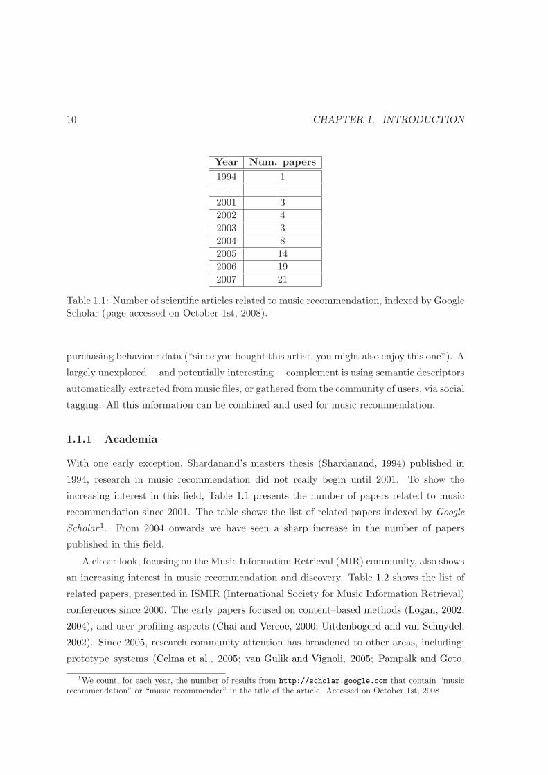
Year Num. papers
1994 1
— —
2001 3
2002 4
2003 3
2004 8
2005 14
2006 19
2007 21
Table 1.1: Number of scientific articles related to music recommendation, indexed by GoogleScholar (page accessed on October 1st, 2008).
purchasing behaviour data (“since you bought this artist, you might also enjoy this one”). A
largely unexplored —and potentially interesting— complement is using semantic descriptors
automatically extracted from music files, or gathered from the community of users, via social
tagging. All this information can be combined and used for music recommendation.
1.1.1 Academia
With one early exception, Shardanand’s masters thesis (Shardanand, 1994) published in
1994, research in music recommendation did not really begin until 2001. To show the
increasing interest in this field, Table 1.1 presents the number of papers related to music
recommendation since 2001. The table shows the list of related papers indexed by Google
Scholar1. From 2004 onwards we have seen a sharp increase in the number of papers
published in this field.
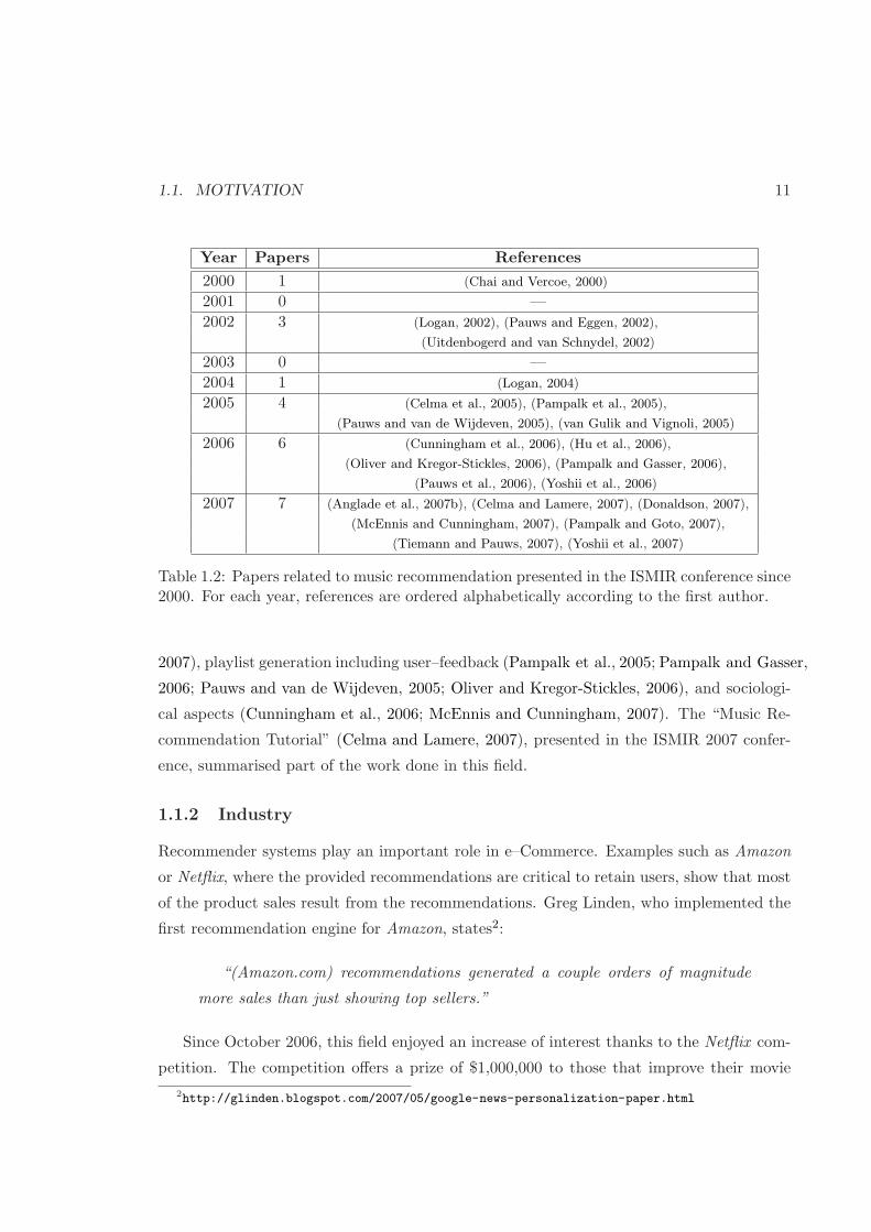
A closer look, focusing on the Music Information Retrieval (MIR) community, also shows
an increasing interest in music recommendation and discovery. Table 1.2 shows the list of
related papers, presented in ISMIR (International Society for Music Information Retrieval)
conferences since 2000. The early papers focused on content–based methods (Logan, 2002,
2004), and user profiling aspects (Chai and Vercoe, 2000; Uitdenbogerd and van Schnydel,
2002). Since 2005, research community attention has broadened to other areas, including:
prototype systems (Celma et al., 2005; van Gulik and Vignoli, 2005; Pampalk and Goto,
1We count, for each year, the number of results from http://scholar.google.com that contain “musicrecommendation” or “music recommender” in the title of the article. Accessed on October 1st, 2008
1.1. MOTIVATION 11
Year Papers References
2000 1 (Chai and Vercoe, 2000)
2001 0 —
2002 3 (Logan, 2002), (Pauws and Eggen, 2002),
(Uitdenbogerd and van Schnydel, 2002)
2003 0 —
2004 1 (Logan, 2004)
2005 4 (Celma et al., 2005), (Pampalk et al., 2005),
(Pauws and van de Wijdeven, 2005), (van Gulik and Vignoli, 2005)
2006 6 (Cunningham et al., 2006), (Hu et al., 2006),
(Oliver and Kregor-Stickles, 2006), (Pampalk and Gasser, 2006),
(Pauws et al., 2006), (Yoshii et al., 2006)
2007 7 (Anglade et al., 2007b), (Celma and Lamere, 2007), (Donaldson, 2007),
(McEnnis and Cunningham, 2007), (Pampalk and Goto, 2007),
(Tiemann and Pauws, 2007), (Yoshii et al., 2007)
Table 1.2: Papers related to music recommendation presented in the ISMIR conference since2000. For each year, references are ordered alphabetically according to the first author.
2007), playlist generation including user–feedback (Pampalk et al., 2005; Pampalk and Gasser,
2006; Pauws and van de Wijdeven, 2005; Oliver and Kregor-Stickles, 2006), and sociologi-
cal aspects (Cunningham et al., 2006; McEnnis and Cunningham, 2007). The “Music Re-
commendation Tutorial” (Celma and Lamere, 2007), presented in the ISMIR 2007 confer-
ence, summarised part of the work done in this field.
1.1.2 Industry
Recommender systems play an important role in e–Commerce. Examples such as Amazon
or Netflix, where the provided recommendations are critical to retain users, show that most
of the product sales result from the recommendations. Greg Linden, who implemented the
first recommendation engine for Amazon, states2:
“(Amazon.com) recommendations generated a couple orders of magnitude
more sales than just showing top sellers.”
Since October 2006, this field enjoyed an increase of interest thanks to the Netflix com-
petition. The competition offers a prize of $1,000,000 to those that improve their movie
2http://glinden.blogspot.com/2007/05/google-news-personalization-paper.html
12 CHAPTER 1. INTRODUCTION
recommendation system3. Also, the Netflix competition provides the largest open dataset,
containing more than 100 million movie ratings from anonymous users. The research com-
munity was challenged in developing algorithms to improve the accuracy of the current
Netflix recommendation system.
State of the Music Industry
The Long Tail4 is composed by a small number of popular items (the hits), and the rest
are located in the tail of the curve (Anderson, 2006). The main goal of the Long Tail
economics —originated by the huge shift from physical media to digital media, and the fall
in production costs— is to make everything available, in contrast to the limitations of the
brick–and–mortar stores. Thus, personalised recommendations and filters are needed to
help users find the right content in the digital space.
On the music side, the 2007 “State of the Industry” report by Nielsen SoundScan
presents some interesting information about music consumption in the United States (Soundscan,
2007). Around 80,000 albums were released in 2007 (not counting music available in Mys-
pace.com, and similar sites). However, traditional CD sales are down 31% since 2004 —but
digital music sales are up 490%. Indeed, 844 million digital tracks were sold in 2007, but
only 1% of all digital tracks accounted for 80% of all track sales. Also, 1,000 albums ac-
counted for 50% of all album sales, and 450,344 of the 570,000 albums sold were purchased
less than 100 times.
Music consumption based on sales is biased towards a few popular artists. Ideally,
by providing personalised filters and discovery tools to users, music consumption would
diversify. There is a need to assist people to discover, recommend, personalise and filter the
huge amount of music content.
1.2 The Problem
Nowadays, we have an overwhelming number of choices of which music to listen to. We
see this each time we browse a non–personalised music catalog, such as Myspace or iTunes.
Schwartz (2005) states that we, as consumers, often become paralyzed and doubtful when
facing the overwhelming number of choices. There is a need to eliminate some of the
3The goal is to reduce by 10% the Root mean squared error (RMSE) of the predicted movies’ ratings4From now on, considered as a proper noun with capitalised letters
1.2. THE PROBLEM 13
choices, and this can be achieved by providing personalised filters and recommendations to
ease users’ decision.
Music 6= movies and books
Several music recommendation paradigms have been proposed in recent years, and many
commercial systems have appeared with more or less success. Most of these approaches
apply or adapt existing recommendation algorithms, such as collaborative filtering, into the
music domain.
However, music is somewhat different from other entertainment domains, such as movies
or books. Tracking users’ preferences is mostly done implicitly, via their listening habits
(instead of asking users to explicitly rate the items). Any user can consume an item (e.g., a
track or a playlist) several times, even repeatedly and continuously. Regarding the evalua-
tion process, music recommendation allows users instant feedback via brief audio excerpts.
The context is another big difference between music and the other two domains. People
consume different music in different contexts; e.g. hard–rock early in the morning, classical
piano sonatas while working, and Lester Young’s cool jazz while having dinner. Thus, a
music recommender has to deal with contextual information.
Predictive accuracy vs. perceived quality
Current music recommendation algorithms try to accurately predict what people will want
to listen to. However, these algorithms tend to recommend popular (or well–known to the
user) artists, which decreases the user’s perceived quality of the recommendations. The
algorithms focus, then, on predicting the accuracy of the recommendations. That is, try to
make accurate predictions about what a user could listen to, or buy next, independently of
how useful the provided recommendations are to the user.
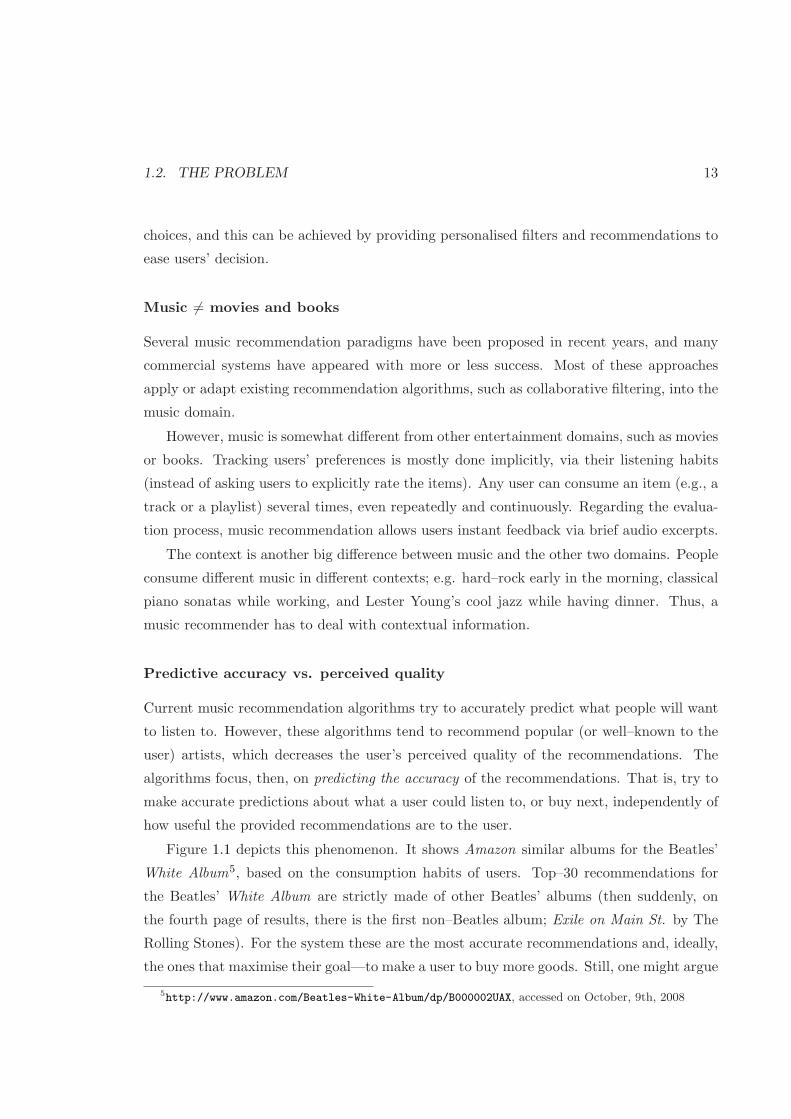
Figure 1.1 depicts this phenomenon. It shows Amazon similar albums for the Beatles’
White Album5, based on the consumption habits of users. Top–30 recommendations for
the Beatles’ White Album are strictly made of other Beatles’ albums (then suddenly, on
the fourth page of results, there is the first non–Beatles album; Exile on Main St. by The
Rolling Stones). For the system these are the most accurate recommendations and, ideally,
the ones that maximise their goal—to make a user to buy more goods. Still, one might argue
5http://www.amazon.com/Beatles-White-Album/dp/B000002UAX, accessed on October, 9th, 2008

14 CHAPTER 1. INTRODUCTION
Figure 1.1: Amazon recommendations for The Beatles’ “White Album”.
about the usefulness of the provided recommendations. In fact, the goals of a recommender
are not always aligned with the goals of a listener. The goal of the Amazon recommender
is to sell goods, whereas the goal for a user visiting Amazon may be to find some new and
interesting music.
1.3 The Solution
The main idea of our solution is to focus on the user’s perceived quality, instead of the
system’s predictive accuracy, of the recommendations. To allow users to discover new music,
recommender systems should exploit the long tail of popularity (e.g., number of total plays,
or album sales) that exists in any large music collection.
Figure 1.2 depicts the long tail of popularity, and how recommender systems should
help us in finding interesting information (Anderson, 2006). Personalised filters assist us in
filtering the available content, and in selecting those —potentially— novel and interesting
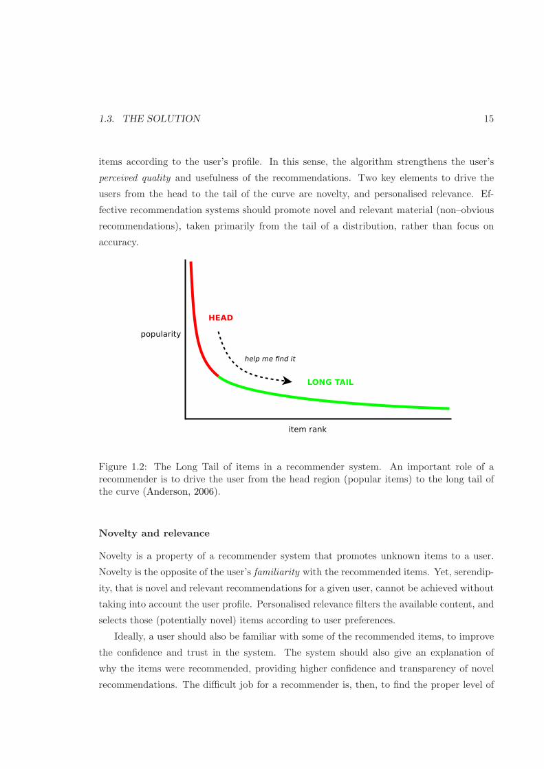
1.3. THE SOLUTION 15
items according to the user’s profile. In this sense, the algorithm strengthens the user’s
perceived quality and usefulness of the recommendations. Two key elements to drive the
users from the head to the tail of the curve are novelty, and personalised relevance. Ef-
fective recommendation systems should promote novel and relevant material (non–obvious
recommendations), taken primarily from the tail of a distribution, rather than focus on
accuracy.
Figure 1.2: The Long Tail of items in a recommender system. An important role of arecommender is to drive the user from the head region (popular items) to the long tail ofthe curve (Anderson, 2006).
Novelty and relevance
Novelty is a property of a recommender system that promotes unknown items to a user.
Novelty is the opposite of the user’s familiarity with the recommended items. Yet, serendip-
ity, that is novel and relevant recommendations for a given user, cannot be achieved without
taking into account the user profile. Personalised relevance filters the available content, and
selects those (potentially novel) items according to user preferences.
Ideally, a user should also be familiar with some of the recommended items, to improve
the confidence and trust in the system. The system should also give an explanation of
why the items were recommended, providing higher confidence and transparency of novel
recommendations. The difficult job for a recommender is, then, to find the proper level of
16 CHAPTER 1. INTRODUCTION
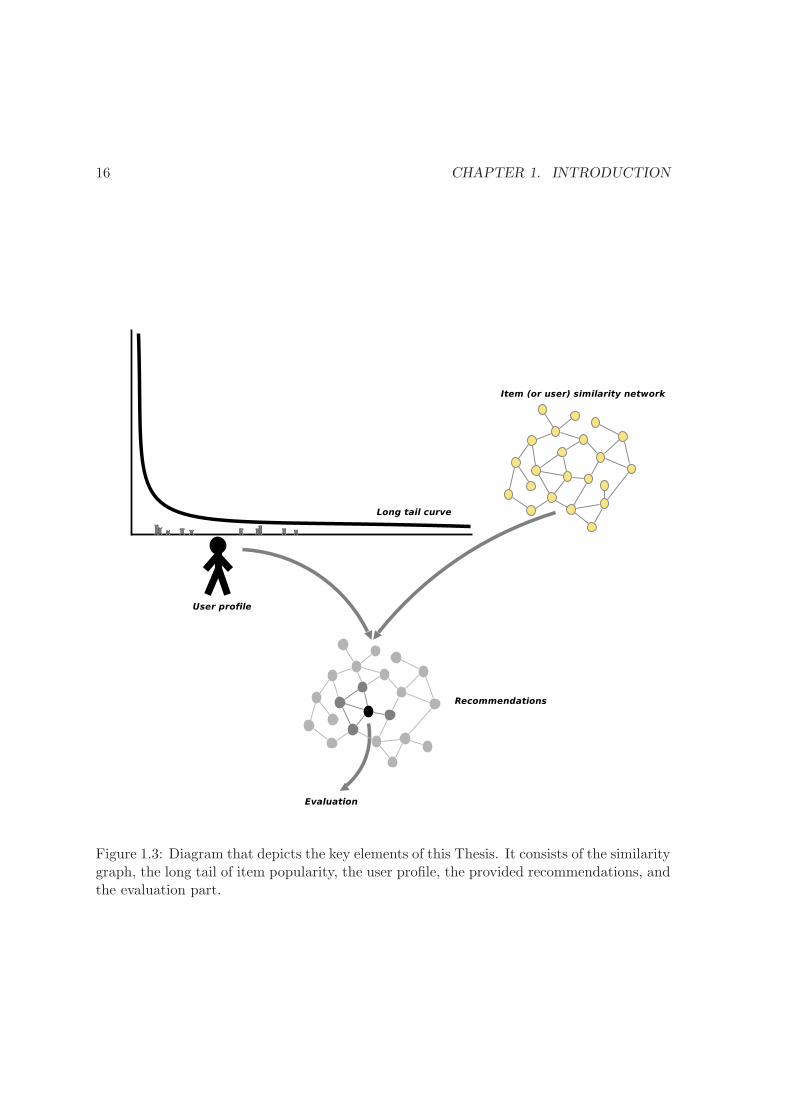
Figure 1.3: Diagram that depicts the key elements of this Thesis. It consists of the similaritygraph, the long tail of item popularity, the user profile, the provided recommendations, andthe evaluation part.
1.4. SUMMARY OF CONTRIBUTIONS 17
familiarity, novelty and relevance for each user. This way, recommendations can use the
long tail of popularity. Furthermore, the proper levels of familiarity, novelty and relevance
for a user will change over time. As a user becomes comfortable with the recommendations,
the amount of familiar items could be reduced.
Proposed approach
Figure 1.3 depicts the main elements involved in this Thesis. The item (or user) similarity
graph defines the relationship among the items (or users). This information is used for
recommending items (or like–minded people) to a given user, based on her preferences. The
long tail curve models the popularity of the items in the dataset, according to the shared
knowledge of the whole community. The user profile is represented along the popularity
curve, using her list of preferred items.
Using the information from the similarity graph, the long tail of item popularity, and the
user profile, we should be able to provide the proper level of familiarity, novelty and relevant
recommendations to the users. Finally, an assessment of the provided recommendations
is needed. This is done in two complementary ways. First, using a novel user–agnostic
evaluation method based on the analysis of the item (or user) similarity network, and the
item popularity. Secondly, with a user–based evaluation, that provides feedback on the list
of recommended items.
1.4 Summary of contributions
The main contributions of this Thesis are:
1. A novel user–agnostic evaluation method (or network–based evaluation) for rec-
ommender systems, based on the analysis of the item (or user) similarity network,
and the item popularity. This method has the following properties:
(a) it measures the novelty component of a recommendation algorithm,
(b) it makes use of complex network analysis to analyse the similarity graph,
(c) it models the item popularity curve,
(d) it combines both the complex network and the item popularity analysis to de-
termine the underlying characteristics of the recommendation algorithm, and
(e) it does not require any user intervention in the evaluation process.
18 CHAPTER 1. INTRODUCTION
We apply this evaluation method to artist, and large–scale user similarity graphs.
2. A user–centric evaluation based on the immediate feedback of the provided rec-
ommendations. This evaluation method has the following advantages (compared to
other system–oriented evaluations):
(a) it measures the novelty factor of a recommendation algorithm in terms of user
knowledge,
(b) it measures the relevance (e.g., like it or not) of the recommendations, and
(c) the users provide immediate feedback to the evaluation system, so the system
can react accordingly.
This method complements the previous, user–agnostic, evaluation approach. We use
this method to evaluate three different music recommendation approaches (social–
based, content–based, and a hybrid approach using expert human knowledge). In
the experiment, 288 subjects rated their personalised recommendations in terms of
novelty (does the user know the recommended song/artist? ), and relevance (does the
user like the recommended song? ).
3. A system prototype, named FOAFing the music, to provide music recommendations
based on the user preferences and her listening habits. The main goal of the Foafing the
Music system is to recommend, to discover and to explore music content; based on user
profiling, context–based information (extracted from music related RSS feeds), and
content–based descriptions (automatically extracted from the audio itself). Foafing
the Music allows users to:
(a) get new music releases from iTunes, Amazon, Yahoo Shopping, etc.
(b) download (or stream) audio from MP3–blogs and Podcast sessions,
(c) discover music with radio–a–la–carte (i.e., personalised playlists),
(d) view upcoming concerts happening near the user’s location, and
(e) read album reviews.
4. A music search engine, named Searchsounds, that allows users to discover unknown
music mentioned on music–related blogs. Searchsounds provides keyword based search,
as well as the exploration of similar songs using audio similarity.
1.5. THESIS OUTLINE 19
1.5 Thesis outline
This Thesis is structured as follows: chapter 2 introduces the basics of the recommendation
problem, and presents the general framework that includes user preferences and represen-
tation. Then, chapter 3 adapts the recommendation problem to the music domain, and
presents related work in this area. Once the users, items, and recommendation methods are
presented, chapter 4 introduces the Long Tail model and its usage in recommender systems.
Chapters 5, 6 and 7 present the different ways of evaluating and comparing different re-
commendation algorithms. Chapter 5 presents the existing metrics for system–, network–,
and user–centric approaches. Then, chapter 6 presents a complement to the classic system–
centric evaluation, focusing on the analysis of the item (or user) similarity network, and
its relationships with the popularity of the items. Chapter 7 complements the previous
approach by entering the users in the evaluation loop, allowing them to evaluate the quality
of the recommendations via immediate feedback. Chapter 8 presents two real prototypes.
These systems, named Searchsounds and FOAFing the music show how to exploit music re-
lated content that is available on the web, for music discovery and recommendation. Finally,
chapter 9 draws some conclusions and discusses open issues and future work.
To summarise the outline of the Thesis, Figure 1.4 presents an extension of Figure 1.3,
including the main elements of the Thesis and its related chapters.

20 CHAPTER 1. INTRODUCTION
Figure 1.4: Extension of Figure 1.3 adding the corresponding chapters.
Chapter 2
The recommendation problem
Generally speaking, the reason people could be interested in using a recommender system is
that they have so many items to choose from—in a limited period of time—that they cannot
evaluate all the possible options. A recommender should be able to bring and filter all this
information to the user. Nowadays, the most successful recommender systems have been
built for entertainment content domains, such as: movies, music, or books (Herlocker et al.,
2004).
This chapter is structured as follows: section 2.1 introduces a formal definition of the
recommendation problem. After that, section 2.2 presents some use cases to stress the
possible usages of a recommender. Section 2.3 presents the general model of the recommen-
dation problem. An important aspect of a recommender system is how to model the user
preferences and how to represent a user profile. This is discussed in section 2.4. After that,
section 2.6 presents some key elements that affect the recommendation problem. Finally,
section 2.5 presents the existing recommendation methods to recommend items (and also
like–minded people) to users.
2.1 Formalisation of the recommendation problem
Intuitively, the recommendation problem can be split into two subproblems. The first one
is a prediction problem, and is about the estimation of the items’ likeliness for a given user.
The second problem is to recommend a list of N items—assuming that the system can pre-
dict likeliness for yet unrated items. Actually, the most relevant problem is the estimation.
Once the system can estimate items into a totally ordered set, the recommendation problem
21

22 CHAPTER 2. THE RECOMMENDATION PROBLEM
reduces to list the top–N items with the highest estimated value.
• The prediction problem can be formalised as follows (Sarwar et al., 2001): Let
U = {u1, u2, . . . um} be the set of all users, and let I = {i1, i2, . . . in} be the set of all
possible items that can be recommended.
Each user ui has a list of items Iui. This list represents the items that the user has
expressed her interests. Note that Iui⊆ I, and it is possible that Iui
be empty1,
Iui= ∅ . Then, the function, Pua,ij is the predicted likeliness of item ij for the active
user ua, such as ij /∈ Iui.
• The recommendation problem is reduced to bringing a list of N items, Ir ⊂ I, that
the user will like the most (i.e the ones with higher Pua,ij value). The recommended
list should not contain items from the user’s interests, i.e. Ir ∩ Iui= ∅.
The space I of possible items can be very large. Similarly, the user space U , can also be
enormous. In most recommender systems, the prediction function is usually represented by a
rating. User ratings are triples 〈u, i, r〉 where r is the value assigned—explicit or implicitly—
by the user u to a particular item i. Usually, this value is a real number (e.g from 0 to 1),
a value in a discrete range (e.g from 1 to 5), or a binary variable (e.g like/dislike).
There are many approaches to solve the recommendation problem. One widely used
approach is when the system stores the interaction (implicit or explicit) between a user and
the item set. The system can provide informed guesses based on the interaction that all the
users have provided. This approximation is called collaborative filtering. Another approach
is to collect information describing the items and then, based on the user preferences, the
system is able to predict which items the user will like the most. This approach is generally
known as content–based filtering, as it does not rely on other users’ ratings but on the
description of the items. Another approach is demographic filtering, that stereotypes the
kind of users that like a certain item. Context–based filtering approach uses contextual
information about the items to describe them. Finally, the hybrid approach combines some
of the previous approaches. Section 2.5 presents all these approaches.
Before presenting the methods to solve the recommendation problem, the following
section explains the most common usages of a recommender. After that, section 2.4 explains
how to model the user preferences.
1Specially when the user creates an account to a recommender system.
2.2. USE CASES 23
2.2 Use cases
Once the recommendation problem has been specified, the next step is to define general
use cases that makes a recommender system useful. Herlocker et al. (2004) identify some
common usages of a recommender:
• Find good items. The aim of this use case is to provide a ranked list of items, along
with a prediction of how much the user would like each item. Ideally, a user would
expect some novel items that are unknown to the user, as well as some familiar items,
too.
• Find all good items. The difference of this use case from the previous one is
with regard the coverage. In this case, the false positive rate should be lower, thus
presenting items with a higher precision.
• Recommend sequence. This use case aims at bringing to the user an ordered
sequence of items that is pleasing as a whole. A paradigmatic example is a music
recommender’s automatic playlist generation.
• Just browsing. In this case, users find pleasant to browse into the system, even if
they are not willing to purchase any item. Simply as an entertainment.
• Find credible recommender. Users do not automatically trust a recommender.
Then, they “play around” with the system to see if the recommender does the job
well. A user interacting with a music recommender will probably search for one of her
favourite artists, and check the output results (e.g. similar artists, playlist generation,
etc.)
• Express self. For some users is important to express their opinions. A recommender
that offers a way to communicate and interact with other users (via forums, weblogs,
etc.) allows the self–expression of users. Thus, other users can get more information—
from tagging, reviewing or blogging processes—about the items being recommended
to them.
• Influence others. This use case is the most negative of the ones presented. There
are some situations where users might want to influence the community in viewing
or purchasing a particular item. E.g: Movie studios could rate high their latest new
release, to push others to go and see the movie. In a similar way, record labels could
try to promote their artists into the recommender.
24 CHAPTER 2. THE RECOMMENDATION PROBLEM
All these use cases are important when evaluating a recommender. The first task of the
evaluators should be to identify the most important use cases for which the recommender
will be used, and based their decisions on that.
2.3 General model
The main elements of a recommender are users and items. Users need to be modelled in a
way that the recommender can exploit their profiles and preferences. Besides, an accurate
description of the items is also crucial to achieve good results when recommending items to
users.
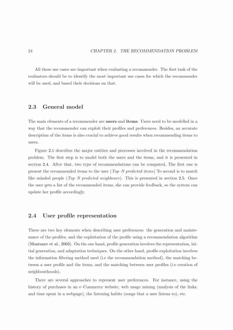
Figure 2.1 describes the major entities and processes involved in the recommendation
problem. The first step is to model both the users and the items, and it is presented in
section 2.4. After that, two type of recommendations can be computed, The first one is
present the recommended items to the user (Top–N predicted items) To second is to match
like–minded people (Top–N predicted neighbours). This is presented in section 2.5. Once
the user gets a list of the recommended items, she can provide feedback, so the system can
update her profile accordingly.
2.4 User profile representation
There are two key elements when describing user preferences: the generation and mainte-
nance of the profiles, and the exploitation of the profile using a recommendation algorithm
(Montaner et al., 2003). On the one hand, profile generation involves the representation, ini-
tial generation, and adaptation techniques. On the other hand, profile exploitation involves
the information filtering method used (i.e the recommendation method), the matching be-
tween a user profile and the items, and the matching between user profiles (i.e creation of
neighbourhoods).
There are several approaches to represent user preferences. For instance, using the
history of purchases in an e–Commerce website, web usage mining (analysis of the links,
and time spent in a webpage), the listening habits (songs that a user listens to), etc.
2.4. USER PROFILE REPRESENTATION 25
Figure 2.1: General model of the recommendation problem.
26 CHAPTER 2. THE RECOMMENDATION PROBLEM
2.4.1 Initial generation
Empty
An important aspect of a user profile is its initialisation. The simplest way is to create an
empty profile, that will be updated as soon as the user interacts with the system. However,
the system will not be able to provide any recommendation until the user has been into the
system for a while.
Manual
Another approach is to manually create a profile. In this case, a system might ask to the
users to register their interests (via tags, keywords or topics) as well as some demographic
information (e.g age, marital status, gender, etc.), geographic data (city, country, etc.) and
psychographic data (interests, lifestyle, etc.). The main drawback is the user’s effort, and
the fact that maybe some interests could still be unknown by the user himself.
Data import
To avoid the manually creation of a profile, the system can ask to the user for available,
external, information that already describes her. In this case, the system only has to
import this information from the external sources that contain relevant information of the
user2. Besides, there have been some attempts to allow users to share their own interests
in a machine–readable format (e.g. XML), so any system can use it and extend it. An
interesting proposal is the Attention Profile Markup Language (APML)3.
The following example4 shows a fragment of an APML file derived from the listening
habits of a last.fm user5. The APML document contains a tag cloud representation created
from the tags defined in the user’s top artists.
<Profile name="music">
<ImplicitData >
<Concepts >
<Concept key="rock" value="1.0" />
2A de–facto standard, in the Semantic Web community, is the Friend of a Friend initiative (FOAF).FOAF provides conventions and a language “to tell” a machine the sort of things that a user says aboutherself. This approach is the one been used in our prototype, presented in chapter 8
3http://www.apml.org4Generated via TasteBroker.org5http://research.sun.com:8080/AttentionProfile/apml/last.fm/ocelma

2.4. USER PROFILE REPRESENTATION 27
Figure 2.2: Example of a pre–defined training set to model user preferences when a usercreates an account in iLike.
<Concept key="hard rock" value="0.41770712" />
<Concept key="sleaze rock" value="0.39724553" />
<Concept key="rock n roll" value="0.3311153" />
<Concept key="glam rock" value="0.23445463" />
<Concept key="classic rock" value="0.2062444" />
<Concept key="singer songwriter" value="0.17533751" />
<Concept key="alternative" value="0.1623969" />
...
</Concepts >
</ImplicitData >
</Profile >
Listing 2.1: Example of a user profile in APML.
28 CHAPTER 2. THE RECOMMENDATION PROBLEM
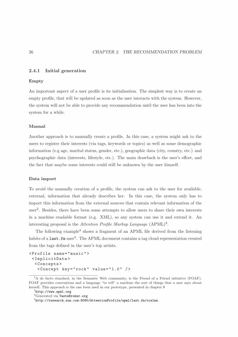
Training set
Another method to gather information is using a pre–defined training set. The user has to
provide feedback to concrete items, marking them as relevant or irrelevant to her interests.
The main problem, though, is to select representative examples. For instance, in the music
domain, the system might ask for concrete genres or styles, and filter a set of artists to be
rated by the user. Figure 2.2 shows an example of the iLike music recommender. Once a
user creates an account, the system presents a list of artists that the user has to rate. This
process is usually perceived by the users as a tedious and unnecessary work. Yet, it gives
some information to the system to avoid the user cold–start problem (see section 2.6 for
more details).
Stereotyping
Finally, the system can gather initial information using stereotyping. This method resembles
to a clustering problem. The main idea is to assign a new user into a cluster of similar users
that are represented by their stereotype, according to some demographic, geographic, or
psychographic information.
2.4.2 Maintenance
Once the profile has been created, it does not remain static. Therefore, user’s interests
might (and probably will) change. A recommender system needs up–to–date information
to automatically update a user profile. Feedback can be explicit or implicit.
Explicit feedback
One option is to ask to the users for relevance feedback about the provided recommenda-
tions. Explicit (positive or negative) feedback usually comes in the form of ratings. This
type of feedback can be positive or negative. Usually, users provide more positive feedback,
although negative examples can be very useful for the system.
Ratings can be in a discrete scale (e.g. from 0 to N), or a binary value (like/dislike).
Yet, it is proved that sometimes users rate inconsistently (Hill et al., 1995), thus ratings
are usually biased towards some values, and this can also depend on the user perception of
the ratings’ scale. Inconsistency in the ratings arouse a natural variability when the system
is predicting the ratings. Herlocker et al. (2004) present a study showing that even best
2.5. RECOMMENDATION METHODS 29
algorithm could not get beyond a Root mean squared error (RMSE) of 0.73, on a five–point
scale. This has strong consequences for recommender systems based on maximising the
predictive accuracy, and also sets a theoretical upper bound to the Netflix competition.
Another way to gather explicit feedback is to allow users to write comments and opinions
about the items. In this case, the system can present the opinions to the target user, along
with the recommendations. This extra piece of information eases the decision–making
process of the target user, although she has to read and interpret other users’ opinions.
Implicit feedback
A recommender can also gather implicit feedback from the user. A system can infer the
user preferences passively by monitoring user’s actions. For instance, by analysing the
history of purchases, the time spent on a webpage, the links followed by the user, the mouse
movements, or analysing a media player usage (tracking the play, pause, skip and stop
buttons).
However, negative feedback is not reliable when using implicit feedback, because the
system can only observe positive (implicit) feedback, by analysing user’s actions. On the
other hand, implicit feedback is not as intrusive as explicit feedback.
2.4.3 Adaptation
As explained in the previous section, relevance feedback implies that the system has to
adapt to the changes of the users’ profiles. The techniques to adapt to new interests and
forget the old ones can be done in three different ways. First, done manually by the user,
although this requires some effort to the user. Secondly, by adding new information into
the user profiles, while keeping the old interests. Finally, by gradually forgetting the old
interests and promoting the new ones (Webb and Kuzmycz, 1996).
2.5 Recommendation methods
Once the user profile is created, the next step is to exploit the user preferences, to provide her
interesting recommendations. User profile exploitation is tightly related with the method for
filtering information. The method adopted for information filtering has led to the standard
classification of recommender systems, that is: demographic filtering, collaborative filtering,
content–based and hybrid approaches. We add another method, named context–based,
30 CHAPTER 2. THE RECOMMENDATION PROBLEM
which recently has grown popularity due to the feasibility of gathering external information
about the items (e.g gathering information from weblogs, analysing the reviews about the
items, etc.).
The following sections present the recommendation methods for one user. It is worth to
mention that another type of (group–based) recommenders also exist. These recommenders
focus on providing recommendations to a group of users, thus trying to maximise the overall
satisfaction of the group (McCarthy et al., 2006; Chen et al., 2008).
2.5.1 Demographic filtering
Demographic filtering can be used to identify the kind of users that like a certain item (Rich,
1979). For example, one might expect to learn the type of person that likes a certain singer
(e.g finding the stereotypical user that listens to Jonas Brothers6 band). This technique
classifies the user profiles in clusters according to some personal data (age, marital status,
gender, etc.), geographic data (city, country) and psychographic data (interests, lifestyle,
etc.). An early example of a demographic filtering system is the Grundy system (Rich, 1979).
Grundy recommended books based on personal information gathered from an interactive
dialogue.
Limitations
The main problems of this method is that a system recommends the same items to people
with similar demographic profiles, so recommendations are too general (or, at least, not
very specific for a given user). Another drawback is the generation of the profile, that
needs some effort from the user. Some approaches try to get (unstructured) information
from user’s webpages, weblogs, etc. In this case, text classification techniques are used to
create the clusters, and classify the users (Pazzani, 1999). All in all, this is the simplest
recommendation method.
2.5.2 Collaborative filtering
The collaborative filtering approach predicts user preferences for items by learning past
user–item relationships. That is, the user gives feedback to the system, so the system
6http://www.jonasbrothers.com/
2.5. RECOMMENDATION METHODS 31
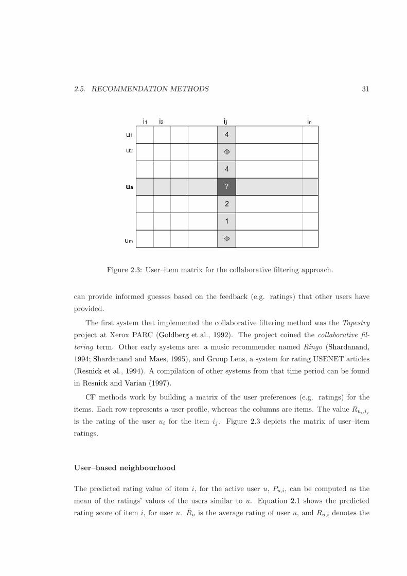
Figure 2.3: User–item matrix for the collaborative filtering approach.
can provide informed guesses based on the feedback (e.g. ratings) that other users have
provided.
The first system that implemented the collaborative filtering method was the Tapestry
project at Xerox PARC (Goldberg et al., 1992). The project coined the collaborative fil-
tering term. Other early systems are: a music recommender named Ringo (Shardanand,
1994; Shardanand and Maes, 1995), and Group Lens, a system for rating USENET articles
(Resnick et al., 1994). A compilation of other systems from that time period can be found
in Resnick and Varian (1997).
CF methods work by building a matrix of the user preferences (e.g. ratings) for the
items. Each row represents a user profile, whereas the columns are items. The value Rui,ij
is the rating of the user ui for the item ij . Figure 2.3 depicts the matrix of user–item
ratings.
User–based neighbourhood
The predicted rating value of item i, for the active user u, Pu,i, can be computed as the
mean of the ratings’ values of the users similar to u. Equation 2.1 shows the predicted
rating score of item i, for user u. Ru is the average rating of user u, and Ru,i denotes the
32 CHAPTER 2. THE RECOMMENDATION PROBLEM
rating of the user u for the item i.
Pu,i = Ru +
∑kv∈Neighbours(u) sim(u, v)(Rv,i − Rv)
∑kv∈Neighbours(u) sim(u, v)
(2.1)
This approach is also known as user–based collaborative filtering.Yet, to predict Pu,i, the
algorithm needs to know beforehand the set of users similar (e.g. like–minded people) to
u, v ∈ Neighbours(u), how similar they are, sim(u, v), and the size of this set, k. This is
analogous to solve the user–profile matching problem (see figure 2.1). The most common
approaches to find the neighbours of u are Pearson correlation (see Equation 2.4), cosine
similarity (see Equation 2.2), and clustering based on stereotypes (Montaner et al., 2003).
Item–based neighbourhood
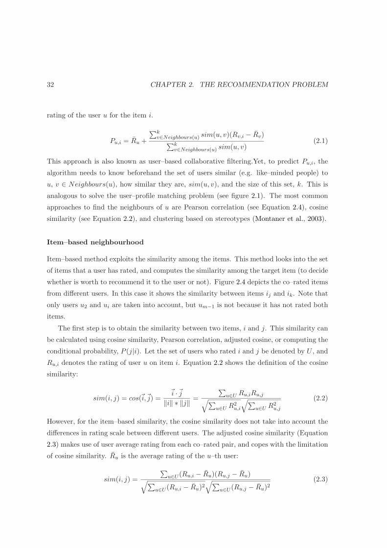
Item–based method exploits the similarity among the items. This method looks into the set
of items that a user has rated, and computes the similarity among the target item (to decide
whether is worth to recommend it to the user or not). Figure 2.4 depicts the co–rated items
from different users. In this case it shows the similarity between items ij and ik. Note that
only users u2 and ui are taken into account, but um−1 is not because it has not rated both
items.
The first step is to obtain the similarity between two items, i and j. This similarity can
be calculated using cosine similarity, Pearson correlation, adjusted cosine, or computing the
conditional probability, P (j|i). Let the set of users who rated i and j be denoted by U , and
Ru,i denotes the rating of user u on item i. Equation 2.2 shows the definition of the cosine
similarity:
sim(i, j) = cos(~i,~j) =~i ·~j
‖i‖ ∗ ‖j‖ =
∑
u∈U Ru,iRu,j√
∑
u∈U R2u,i
√
∑
u∈U R2u,j
(2.2)
However, for the item–based similarity, the cosine similarity does not take into account the
differences in rating scale between different users. The adjusted cosine similarity (Equation
2.3) makes use of user average rating from each co–rated pair, and copes with the limitation
of cosine similarity. Ru is the average rating of the u–th user:
sim(i, j) =
∑
u∈U (Ru,i − Ru)(Ru,j − Ru)√
∑
u∈U (Ru,i − Ru)2√
∑
u∈U (Ru,j − Ru)2(2.3)
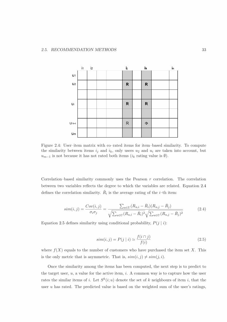
2.5. RECOMMENDATION METHODS 33
Figure 2.4: User–item matrix with co–rated items for item–based similarity. To computethe similarity between items ij and ik, only users u2 and ui are taken into account, butum−1 is not because it has not rated both items (ik rating value is ∅).
Correlation–based similarity commonly uses the Pearson r correlation. The correlation
between two variables reflects the degree to which the variables are related. Equation 2.4
defines the correlation similarity. Ri is the average rating of the i–th item:
sim(i, j) =Cov(i, j)
σiσj=
∑
u∈U (Ru,i − Ri)(Ru,j − Rj)√
∑
u∈U (Ru,i − Ri)2√
∑
u∈U (Ru,j − Rj)2(2.4)
Equation 2.5 defines similarity using conditional probability, P (j | i):
sim(i, j) = P (j | i) ≃ f(i ∩ j)
f(i)(2.5)
where f(X) equals to the number of customers who have purchased the item set X. This
is the only metric that is asymmetric. That is, sim(i, j) 6= sim(j, i).
Once the similarity among the items has been computed, the next step is to predict to
the target user, u, a value for the active item, i. A common way is to capture how the user
rates the similar items of i. Let Sk(i; u) denote the set of k neighbours of item i, that the
user u has rated. The predicted value is based on the weighted sum of the user’s ratings,

34 CHAPTER 2. THE RECOMMENDATION PROBLEM
∀j ∈ Sk(i; u). Equation 2.6 shows the predicted value for item i to user u.
Pu,i =
∑
j∈Sk(i;u) sim(i, j)Ru,j∑
j∈Sk(i;u) sim(i, j)(2.6)
Limitations
Collaborative filtering is one of the most used methods of existing social–based recommender
systems, yet the approach presents some drawbacks:
• Data sparsity and high dimensionality are two inherent properties of the datasets.
With a relative large number of users and items, the main problem is the low coverage
of the users’ ratings among the items. It is common to have a sparse user–item matrix
of 1% coverage. Thus, sometimes it can be difficult to find reliable neighbours (for
user–based CF).
• Another problem, related with the previous one, is that the users with atypical tastes
(that vary from the norm) will not have many users as neighbours. Thus, this
will lead to poor recommendations. This problem is also known as gray sheep
(Claypool et al., 1999).
• Cold–start problem This problem appears for both elements of a recommender:
users and items. Due to CF is based on users’ ratings, new users with only a few ratings
become more difficult to categorise. The same problem occurs with new items, because
they do not have many ratings when they are added to the collection. A related
problem occurs for new items. These cannot be recommended until the users start
rating it. This problem is known as the early–rater problem (Avery and Zeckhauser,
1997). Moreover, the first user that rates new items gets only little benefit (this new
item does not match with any other item yet).
• CF is based only on the feedback provided by the users (in terms of ratings, purchases,
downloads, etc.), and does not take into account the description of the items. It is a
subjective method that aggregates the social behaviour of the users, thus commonly
leading towards recommending the most popular items.
• Related with the previous issue, the popularity bias is another problem that com-
monly happens in CF. It is analogous to the “rich gets richer” paradigm. Popular
items of the dataset are similar to (or related with) lots of items. Thus, it is more
probable that the system recommends these popular items. This clearly happens for
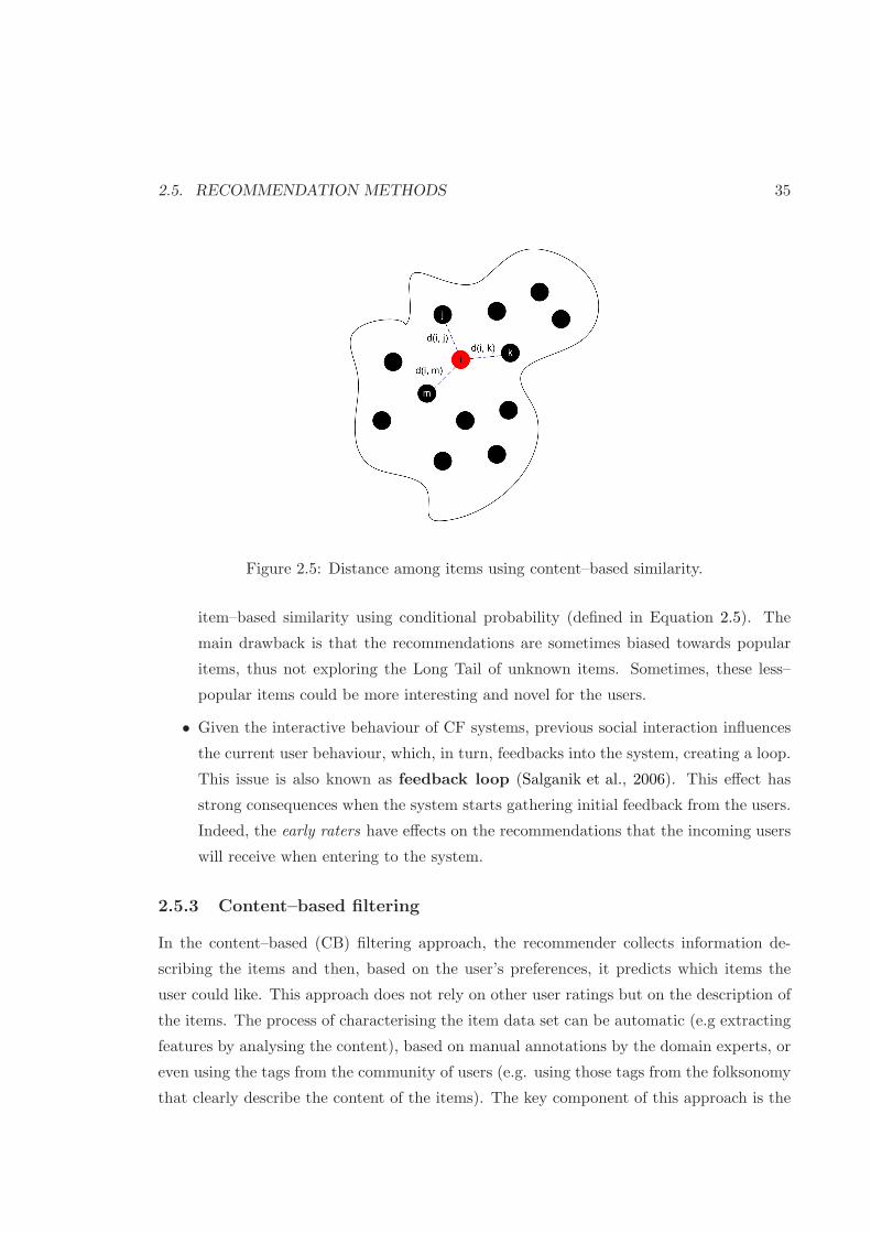
2.5. RECOMMENDATION METHODS 35
Figure 2.5: Distance among items using content–based similarity.
item–based similarity using conditional probability (defined in Equation 2.5). The
main drawback is that the recommendations are sometimes biased towards popular
items, thus not exploring the Long Tail of unknown items. Sometimes, these less–
popular items could be more interesting and novel for the users.
• Given the interactive behaviour of CF systems, previous social interaction influences
the current user behaviour, which, in turn, feedbacks into the system, creating a loop.
This issue is also known as feedback loop (Salganik et al., 2006). This effect has
strong consequences when the system starts gathering initial feedback from the users.
Indeed, the early raters have effects on the recommendations that the incoming users
will receive when entering to the system.
2.5.3 Content–based filtering
In the content–based (CB) filtering approach, the recommender collects information de-
scribing the items and then, based on the user’s preferences, it predicts which items the
user could like. This approach does not rely on other user ratings but on the description of
the items. The process of characterising the item data set can be automatic (e.g extracting
features by analysing the content), based on manual annotations by the domain experts, or
even using the tags from the community of users (e.g. using those tags from the folksonomy
that clearly describe the content of the items). The key component of this approach is the

36 CHAPTER 2. THE RECOMMENDATION PROBLEM
similarity function among the items (see Figure 2.5).
Initial CB approaches have its roots in the information retrieval (IR) field. The early
systems focused on the text domain, and applied techniques from IR to extract meaningful
information from the text. Yet, recently have appeared some solutions that cope with more
complex domains, such as music. This has been possible, partly, because the multime-
dia community emphasised on and improved the feature extraction and machine learning
algorithms algorithms.
The similarity function computes the distance between two items. Content–based simi-
larity focus on an objective distance among the items, without introducing any subjective
factor into the metric (as CF does). Most of the distance metrics deal with numeric at-
tributes, or single feature vectors. Some common distances, given two feature vectors x and
y, are: Euclidean (Equation 2.7), Manhattan (equation 2.8), Chebychev (Equation 2.9),
cosine distance for vectors (see previously defined Equation 2.2), and Mahalanobis distance
(Equation 2.10).
d(x, y) =
√
√
√
√
n∑
i=1
(xi − yi)2 (2.7)
d(x, y) =n
∑
i=1
|xi − yi| (2.8)
d(x, y) = maxi=1..n|xi − yi| (2.9)
d(x, y) =√
(x − y)T S−1(x − y) (2.10)
Euclidean, Manhattan and Chebychev distance are assuming that the attributes are or-
thogonal. The Mahalanobis distance is more robust to the dependencies among attributes,
as it uses the covariance matrix S.
If the attributes are nominal (not numeric), a delta function can be used. A simple
definition of a delta function could be: δ(a, b) = 0 ⇔ a = b, and δ(a, b) = 1 otherwise.
Then, a distance metric among nominal attributes can be defined as (where ω is a reduction
2.5. RECOMMENDATION METHODS 37
factor, e.g 1n):
d(x, y) = ωn
∑
i=1
δ(xi, yi) (2.11)
Finally, if the distance to be computed has to cope with both numeric and nominal at-
tributes, then the final distance has to combine two equations (2.11 for nominal attributes
and one of 2.7. . . 2.10 for numeric attributes).
In some cases, items are not modelled with a single feature vector, but using a bag–
of–vectors, a time series, or a probability distribution over the feature space (section 3.4.2
presents some examples of similarity metrics using more complex data than a single feature
vector).
Yet, similarity measures are not always objective. In some domains, similarity is very
context–dependent. Actually, the subjective part is a big factor of the measure, and these
measures do not take this into account. There are several context–dependent elements that
should be considered (e.g. to whom?, when?, where?, and specially why? ).
Limitations
CB approach presents some drawbacks:
• The cold–start problem occurs when a new user enters to the system. The system
has yet to adapt to the user preferences.
• The gray–sheep problem (users with atypical tastes) can occur, too, depending on
the size of the collection, or if the collection is biased towards a concrete genre.
• Another potential caveat could be the novelty problem. Assuming that the similarity
function works accurately, then one might assume that a user will always receive items
too similar to the ones in her profile. To cope with this shortcoming, the recommender
should use other factors to promote the eclecticness of the recommended items.
• Depending on the domain complexity, another drawback is the limitation of the fea-
tures that can be (automatically) extracted from the objects. For instance in the
multimedia arena, nowadays, is still difficult to extract high–level descriptors with a
clear meaning for the user. Music analysis is not ready yet to accurately predict the
mood but, on the other hand, it does the job well when dealing with descriptors such
as: harmony, rhythm, etc. Thus, an item description is not close enough to the user,
38 CHAPTER 2. THE RECOMMENDATION PROBLEM
but still the automatic description is useful to compute item similarity (e.g songs).
• Another shortcoming is that the recommender is focused on finding similarity among
items, using only the features describing the items. The method is limited by the
features that are explicitly associated with the items. This means that subjectivity
(or personal opinions) is not taken into account when recommending items to users.
CB methods solve some of the shortcomings of the collaborative filtering. The early–
rater problem disappears. When adding a new item into the collection—and computing
the similarity among the rest of the items—it can be recommended without being rated by
any user. The popularity bias is solved too. Because there is no human intervention in the
process, all the items are considered (in principle) to be of equal importance.
2.5.4 Context–based filtering
Context vs. content
Context is any information that can be used to characterise the situation of an entity
(Abowd et al., 1999). Context–based recommendation uses, then, contextual information
to describe and characterise the items. To compare content and context–based filtering, a
clear example is the different methods used for email spam detection. The common one is
based on the text analysis of the mail (i.e. content–based), whereas context filtering does
not deal with the content of the mail. It rather uses the context of the SMTP connection
to decide whether an email should be marked as spam or not.
In this section, we briefly outline two techniques, Web mining and Social tagging, that
can be used to derive similarity among the items (or user), and also can provide effective
recommendations. Web mining is based on analysing the available content on the Web, as
well as the usage and interaction with the content. Social tagging mines the information
gathered from a community of users that annotate (tag) the items.
Web Mining
Web mining techniques aim at discovering interesting and useful information from the anal-
ysis of the content and its usage. Kosala and Blockeel (2000) identify three different web
mining categories: content, structure and usage mining.
• Web content mining includes text, hypertext, markup, and multimedia mining.
From the analysis of the content, item similarity can be derived. Some examples
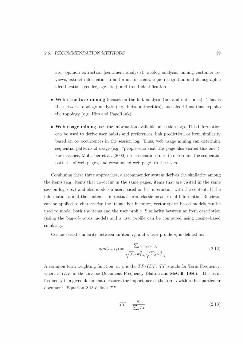
2.5. RECOMMENDATION METHODS 39
are: opinion extraction (sentiment analysis), weblog analysis, mining customer re-
views, extract information from forums or chats, topic recognition and demographic
identification (gender, age, etc.), and trend identification.
• Web structure mining focuses on the link analysis (in– and out– links). That is
the network topology analysis (e.g. hubs, authorities), and algorithms that exploits
the topology (e.g. Hits and PageRank).
• Web usage mining uses the information available on session logs. This information
can be used to derive user habits and preferences, link prediction, or item similarity
based on co–occurrences in the session log. Thus, web usage mining can determine
sequential patterns of usage (e.g. “people who visit this page also visited this one”).
For instance, Mobasher et al. (2000) use association rules to determine the sequential
patterns of web pages, and recommend web pages to the users.
Combining these three approaches, a recommender system derives the similarity among
the items (e.g. items that co–occur in the same pages, items that are visited in the same
session log, etc.) and also models a user, based on her interaction with the content. If the
information about the content is in textual form, classic measures of Information Retrieval
can be applied to characterise the items. For instance, vector space–based models can be
used to model both the items and the user profile. Similarity between an item description
(using the bag–of–words model) and a user profile can be computed using cosine–based
similarity.
Cosine–based similarity between an item ij , and a user profile ui is defined as:
sim(ui, ij) =
∑
t wt,uiwt,ij
√
∑
t w2t,ui
√
∑
t w2t,ij
(2.12)
A common term weighting function, wi,j , is the TF/IDF . TF stands for Term Frequency,
whereas IDF is the Inverse Document Frequency (Salton and McGill, 1986). The term
frequency in a given document measures the importance of the term i within that particular
document. Equation 2.13 defines TF :
TF =ni
∑
k nk(2.13)
40 CHAPTER 2. THE RECOMMENDATION PROBLEM
with ni being the number of occurrences of the considered term, and the denominator is
the number of occurrences of all the terms in the document.
The Inverse Document Frequency, IDF , measures the general importance of the term,
in the whole collection of items:
IDF = log|D|
|(di ⊃ ti)|(2.14)
where |D| is the total number of items, and the denominator counts the number of items
where ti appears. Finally, the weighting function wt,j , of a term t in the item description
dj is computed as:
wt,j = TF · IDF (2.15)
Another useful measure to compute item similarity is the Pointwise mutual information
(PMI). PMI estimates the semantic similarity between a pair of terms by how frequently
they co–occur. The PMI of two terms i and j quantifies the discrepancy between their joint
distribution probability, versus their individual distribution probability (assuming indepen-
dence):
PMI(i, j) = logp(i, j)
p(i)p(j)(2.16)
PMI measure is symmetric, that is PMI(x, y) = PMI(y, x).
Social tagging
Social tagging (also known as Folksonomy, or Collaborative tagging) aims at annotating
web content using tags. Tags are freely chosen keywords, not constrained to a predefined
vocabulary. A bottom–up classification emerge when grouping all the annotations (tags)
from the community of users. Mining social tagging data can help recommender systems
to derive item (or user) similarity.
When users tag items, we get tuples of 〈user, item, tag〉. These triples conform a 3–order
matrix (also called tensor, a multidimensional matrix). Figure 2.6 depicts a 3–order tensor,
containing the tags that the users apply to the items.
There are two main approaches to use social tagging information in recommendation:
1. Unfold the 3–order tensor in three bidimensional matrices (user–tag, item–tag and
2.5. RECOMMENDATION METHODS 41
Figure 2.6: 3–order tensor containing 〈user, item, tag〉 triples.
user–item matrices), and
2. Directly use the 3–order tensor.
Unfolding the 3–order tensor consists on decomposing the multidimensional data into
the following bidimensional matrices:
• User–Tag (U matrix). Ui,j contains the number of times user i applied the tag
j. Using matrix U , a recommender system can derive a user profile (e.g. a tag
cloud for each user, denoting her interests, or the items she tags). U can also be
used to compute user similarity, comparing two user tag clouds of interests, and
using cosine similarity of the two vectors.
• Item–Tag (I matrix). Ii,j contains the number of times an item i has been
tagged with tag j. The matrix I contains the contextual description of the items,
based on the tags that have been applied to. Matrix I can be used to compute
item or user similarity. As an example, Figure 2.7 shows a way to derive user
similarity from I. Figure 2.7 depicts two user tag clouds (top and middle images)
and their intersection (bottom image), using matrix I. In this example, users’
tag clouds are derived from the last.fm listening habits, using their top–N most
listened artists —in this case, the items in I. The third image (bottom) shows
the tags that co-occur the most in the two profiles. Similarity between the two
users is done by constructing a new tag vector where each tag’s weight is given
by the minimum of the tag’s weights in the user’s vectors. Using this approach,

42 CHAPTER 2. THE RECOMMENDATION PROBLEM
Figure 2.7: Two examples of users’ tag clouds derived from their last.fm listen-ing habits. Top and middle images show two last.fm user tag clouds. The thirdimage (bottom) shows the tags that co-occur the most in the two profiles. Ac-cording to Anthony Liekens’ algorithm, the similarity value between ocelma andlamere last.fm users is 70.89%. Image courtesy of Anthony Liekens, taken fromhttp://anthony.liekens.net/pub/scripts/last.fm/compare.php.
2.5. RECOMMENDATION METHODS 43
the similarity value between ocelma and lamere last.fm users is 70.89%. Another
similarity metric could be the cosine distance, using TFxIDF to weight each tag.
• User–Item (R binary matrix). Ri,j denotes whether the user i has tagged the
item j. In this case, classic collaborative filtering techniques can be applied on
top of R.
To recap, item similarity using I, or user similarity derived from U or I, can be
computed using cosine–based distance (see Equation 2.2), or also by applying dimen-
sionality reduction techniques —to deal with the sparsity problem—, such as Singular
Value Decomposition (SVD), or Non–negative matrix factorisation (NMF).
Once the item (or user) similarity is computed, either the R user–item matrix, or the
user profile (tag cloud) obtained from U or I are used to predict the recommendations
for a user. For instance, Ji et al. (2007) present a framework based on the three
matrices, U , I and R, to recommend web pages (based on http://del.icio.us data).
Also, Tso-Sutter et al. (2008) uses matrix I to improve the accuracy results of the
recommendations, after combining I with the results obtained by classic collaborative
filtering. Levy and Sandler (2007) applies Latent Semantic Analisys (that is; SVD
and cosine similarity in the reduced space) to compute and visualise artist similarity
derived from tags gathered from last.fm.
Finally, it is worth mentioning that inverting either U or I matrices, one can also
compute tag similarity. Tag similarity have many usages in recommendation and
search engines. For instance, tag synonym detection can be used for query expansion,
or tag suggestion when annotating the content.
Using the 3–order tensor (instead of decomposing the tensor in bidimensional matrices)
is the second approach to mine the data, and provide recommendations. The avail-
able techniques are (high–order) extensions of SVD and NMF. HOSVD is a higher
order generalisation of matrix SVD for tensors, and Nonnegative Tensor Factorisation
(NTF) is a generalisation of NMF.
Symeonidis et al. (2008) apply HOSVD to a music dataset (user–artists–tags) taken
from last.fm. Their results show significant improvements in terms of the effectiveness
measured through precision and recall. Xu et al. (2006) present a similar method
using bookmarking data from del.icio.us. They apply SVD on the R matrix, compute
cosine distance among the users (to find the neighbours), and then apply classic
44 CHAPTER 2. THE RECOMMENDATION PROBLEM
CF user–based recommendation (see section 2.5.2). The authors could improved the
results over a CF approach based on SVD and cosine similarity (e.g. Latent Semantic
Analysis).
Limitations of Social Tagging
One of the main limitations of social tagging is the coverage. It is quite common that only
the most popular items are described by several users, creating a compact description of the
item. On the other hand, long tail items usually do not have enough tags to characterise
them. This makes the recommendation process very difficult, specially to promote these
unknown items.
Another issue is that without being constrained to a controlled vocabulary, tags present
the following problems: polysemy (I love this song, versus this song is about love), synonymy
(hip–hop, hiphop, and rap), and usefulness of the personal to derive similarity among users
or items (e.g. seen live, or to check). This issues make more difficult to mine and extract
useful relationships among the items and the users.
Finally, tag usage is another problem. In some domains, some tags are widely used (e.g.
rock, in the music domain), whereas other tags are rarely applied (e.g. gretsch guitar). A
biased distribution of the terms has also consequences when exploiting social tagging data.
2.5.5 Hybrid methods
The main purpose of a hybrid method is to achieve a better prediction by combining some
of the previous stand–alone approaches. Most commonly, collaborative filtering is combined
with other techniques. There are different methods to integrate different approaches into a
hybrid recommender. Burke (2002) defines the following methods:
• Weighted. A hybrid method that combines the output of separate approaches using,
for instance, a linear combination of the scores of each recommendation technique.
• Switching. The system uses some criterion to switch between recommendation tech-
niques. One possible solution is that the system uses a technique, and if the results are
not confident enough, it switches to another technique to improve the recommendation
process.
• Mixed. In this approach, the recommender does not combine but expand the de-
scription of the data sets by taking into account the users’ ratings and the description
2.6. FACTORS AFFECTING THE RECOMMENDATION PROBLEM 45
of the items. The new prediction function has to cope with both types of descriptions.
• Cascade. The cascade involves a step by step process. In this case, a recommenda-
tion technique is applied first, producing a coarse ranking of items. Then, a second
technique refines or re–rank results obtained in the first step.
A hybrid method can alleviate some of the drawbacks that suffer a single technique.
2.6 Factors affecting the recommendation problem
Novelty and serendipity
The novelty factor is a very important aspect of the recommendation problem. It has
been largely acknowledged that providing obvious recommendations can decrease user sat-
isfaction (Herlocker et al., 2004; McNee et al., 2006). Obvious recommendations have two
practical disadvantages: users who are interested in those items could probably already
know them, and secondly, managers in stores (i.e experts of the items’ domain) do not need
any recommender to tell them which products are popular overall.
Although, obvious recommendations do have some value for new users. Users like to
receive some recommendations they already are familiar with (Swearingen and Sinha, 2001).
This is related with the Find credible recommender use case (see Section 2.2). Yet, there
is a trade–off between the desire for novelty and familiar recommendations. A high novelty
rate might mean, for a user, that the quality of the recommendation is poor, because the
user is not be able to identify most of the items in the list of recommendations. However,
by providing explanations (transparency) of the recommendations, the user can feel that
is a credible recommender. Thus, the user can be more open to receive novel, justified,
recommendations.
Another important feature, closely related with novelty is the serendipity effect. That
is the good luck in making unexpected and fortunate discoveries. A recommender should
help the user to find a surprisingly interesting item that she might not be able to discover
otherwise. Recommendations that are serendipitous are also novel and relevant for a user.
Explainability
Explainability (or transparency) of the recommendations is another important element.
Giving explanations about the recommended items could increase user trustiness and loyalty
46 CHAPTER 2. THE RECOMMENDATION PROBLEM
of the system, and also her satisfaction.
A recommender should be able to explain to the user why the system recommends
the list of top–K items (Sinha and Swearingen, 2002). Herlocker et al. (2000) presents
an experimental evidence that shows that providing explanations can improve the accep-
tance of the recommender systems based on CF. Actually, giving explanations about why
the items were recommended is as important as the actual list of recommended items.
Tintarev and Masthoff (2007) summarise the possible aims to providing explanations about
the recommendations. These are: transparency, scrutability, trust, effectiveness, persuasive-
ness, efficiency, and satisfaction. The authors also stress the importance of personalising
the explanations to the user.
Cold start problem
The cold start problem of a recommender (also known as the learning rate curve, or the
bottleneck problem) happens when a new user (or a new item) enters into the system
(D.Maltz and Ehrlich, 1995). On the one hand, cold start is a problem for the new users
that start playing around with the system, because the system does not have enough in-
formation about them. If the user profile initialisation is empty (see section 2.4.1), she has
to dedicate an amount of effort using the system before getting some reward (i.e. useful
recommendations). On the other hand, when a new item is added to the collection, the
system should have enough information to be able to recommend this item to the users.
Data sparsity and high dimensionality
Data sparsity is an inherent property of the dataset. With a relative large number of users
and items, the main problem is the low coverage of the users’ interaction with the items.
A related factor is the high dimensionality of the dataset, that consists of many users and
items.
There are some methods, based on dimensionality reduction, to alleviate data sparsity
and the high dimensionality of the dataset. Singular Value Decomposition (SVD), and Non–
negative Matrix Factorisation (NMF) (Paatero and Tapper, 1994; Lee and Seung, 1999) are
the two most used methods in recommendation. Also in (Takacs et al., 2008), the authors
present several matrix factorisation algorithms, and they evaluate the results against the
Netflix Prize dataset.

2.6. FACTORS AFFECTING THE RECOMMENDATION PROBLEM 47
Coverage
The coverage of a recommender measures the percentage of the items in the collection
over which the system can form predictions, or make recommendations. A low coverage
of the domain might be less valuable to users, as it limits the space of possible items to
recommend. Moreover, this feature is important for the Find all good items use case (see
section 2.2). Also, a low coverage of the collection can be very frustrating for the users, and
clearly affects the novelty and serendipity factors.
Trust
Trust–aware recommender systems determine which users are reliable, and which are not.
Trust computational models are needed, for instance, in user–based CF to rely on the user’s
neighbours.
O’Donovan and Smyth (2005) present two computational models of trust and show how
they can be readily incorporated into CF. Furthermore, combining trust and classic CF can
improve the predictive accuracy of the recommendations. In (Massa and Avesani, 2007),
the authors emphasise the “web of trust” provided by every user. The authors use the
“web of trust” to propagate trust among users, and also use it to alleviate the data sparsity
problem. An empirical evaluation shows that using trust information predictive accuracy
improves, as well as the coverage of the recommendations.
Temporal effects
Temporal effect play an important role in recommender systems. The timestamp of an
item (e.g. when was the item added to the collection) is an important factor for the
recommendation algorithm. The prediction function should take into account the age of
the items. A common approach is to treat the older items as less relevant than the new
ones.
Also, the system has to decide which items from the user profile are taken into account
to do the predictions. Should the system use all the information of a user, or only the latest
one? This can clearly change the provided recommendations. In this context, Shani et al.
(2002) present the recommender problem as a sequential optimisation problem. It is based
on Markov decision processes (MDP). MDP uses the long–term effects of the recommenda-
tions, but it is also configurable to use only the last k–actions of a user. The main problem,
48 CHAPTER 2. THE RECOMMENDATION PROBLEM
though is the computationally complexity of the algorithm, which makes it unusable for
large datasets.
Understanding the users
Modelling user preferences, including psychographic information is another challenging
problem. Psychographic variables include attributes related with personality, such as atti-
tudes, interests, or lifestyles. It is not straightforward to encode all this information and
make it useful for a system. This problem is similar in Information Retrieval (IR) systems;
to express the user needs via a keyword–based query. There is always a loss of information
when a user is formulating a query using a language that the machine can understand and
process.
2.7 Summary
This chapter has presented and formalised the recommendation problem. The main com-
ponents of a recommender are the users and the items. Based on the user preferences and
the exploitation of a user profile, a recommender can solve the problem of recommending
items to users. There are several factors that affect the recommendation problem. In this
thesis we specially focus on the novelty one. We believe that this is an important topic that
deserves to be analysed in depth. To recap, Table 2.7 presents the main elements involved
in the recommendation problem, that is user profiling, and the recommendation methods.
Then, chapter 3 applies all these concepts in the music recommendation domain. Fur-
thermore, the special requirements to solve the music recommendation problem are pre-
sented too.
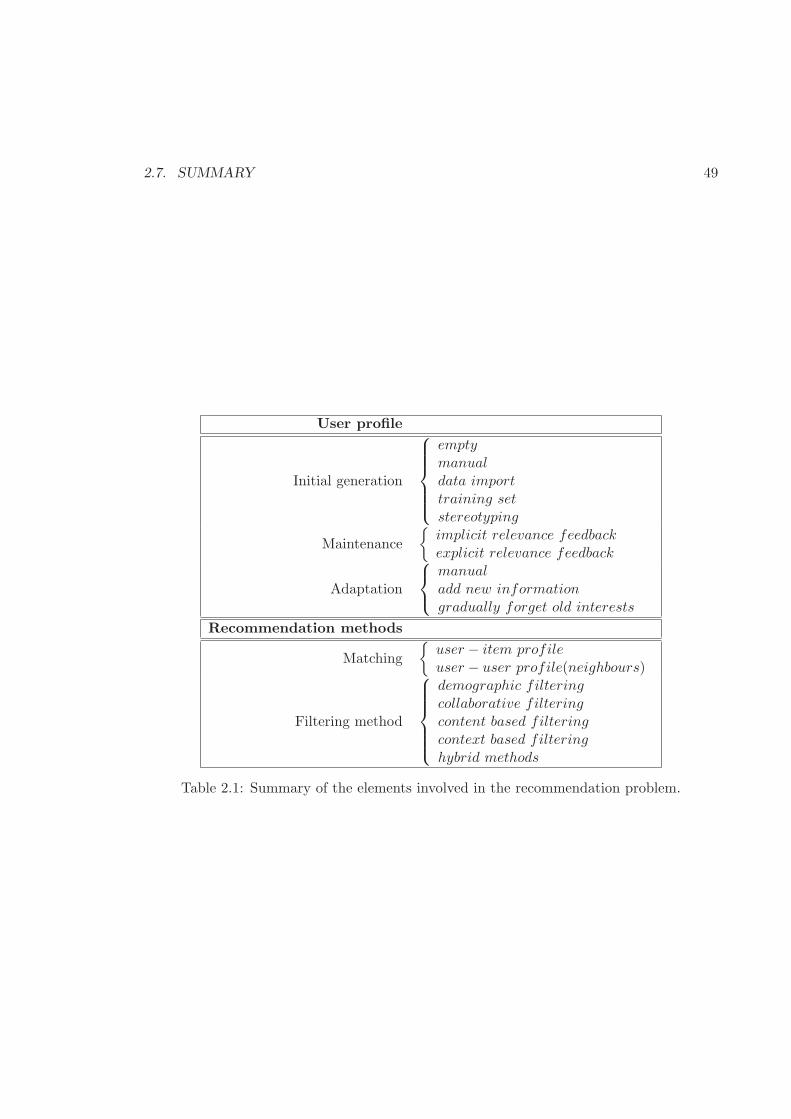
2.7. SUMMARY 49
User profile
Initial generation
emptymanualdata importtraining setstereotyping
Maintenance
{
implicit relevance feedbackexplicit relevance feedback
Adaptation
manualadd new informationgradually forget old interests
Recommendation methods
Matching
{
user − item profileuser − user profile(neighbours)
Filtering method
demographic filteringcollaborative filteringcontent based filteringcontext based filteringhybrid methods
Table 2.1: Summary of the elements involved in the recommendation problem.

50 CHAPTER 2. THE RECOMMENDATION PROBLEM
Chapter 3
Music recommendation
This chapter presents the music recommendation problem. Section 3.1 presents some com-
mon use cases in the music domain. After that, section 3.2, discusses user profiling and
modelling, and how to link the components of a user profile with the music concepts. Then,
section 3.3 presents the elements that describe the musical items (i.e. artists and songs). The
existing music recommendation methods (collaborative filtering, content, context–based,
and hybrid) are presented in section 3.4. Finally, section 3.5 summarises the work in this
area, and provides some links with the remaining chapters of the Thesis.
3.1 Use Cases
The main task of a music recommendation system is to propose to the user interesting music
to discover, including unknown artists and their available tracks, based on the user’s musical
taste. Music is somewhat different from other entertainment domains, such as movies, or
books. Tracking user preferences is done implicitly, via her listening habits. Usually explicit
feedback is not gathered in terms of ratings, but in terms of playing, skipping, or stopping
a recommended track.
Most of the work done in music recommendation focuses on presenting to a user a list
of artists, or creating an ordered sequence of songs (a personalised playlist). To achieve
this, the most common approaches are based on collaborative filtering and audio content–
based filtering. Yet, recently have appeared other (context–based) approaches such as social
tagging, and music web mining that can also be used for that purpose.
51
52 CHAPTER 3. MUSIC RECOMMENDATION
3.1.1 Artist recommendation
According to the general model presented in chapter 2 (see Figure 2.1), artist recommen-
dation follows the user–item matching, were items are recommended to a user according to
her profile. However, artist recommendation should involve a broader experience with the
user, more than presenting a list of relevant artists, and the associated metadata.
In this sense, there is a lot music related information on Internet: music performed by
“unknown” –long tail— artists that can suit perfectly for new recommendations, new music
releases, related news, announcements of concerts, album reviews, mp3–blogs, podcast ses-
sions, etc. Indeed, music websites syndicate (part of) their web content—noticing the user
about new releases, artist’s related news, upcoming gigs, etc.—in the form of RSS (Really
Simple Syndication) feeds. For instance, the iTunes Music Store1 provides an RSS feed
generator2 updated once a week, that publishes all the new releases of the week.
A music recommendation system should take advantage of these publishing services, as
well as integrating them into the system, to filter and recommend music related information
to the user.
3.1.2 Neighbour recommendation
The goal of neighbour recommendation is to find like–minded people, and through them
discover unknown and interesting music. Neighbour similarity can be computed using the
user–user profile matching presented in Figure 2.1.
One of the main advantages of creating neighbourhoods is that a user can explore her
similar users, easing the music discovery process. Also, it permits the creation of social
networks, connecting people that share similar interests.
3.1.3 Playlist generation
Playlist generation is an important application in music recommendation, as it allows users
to listen to the music as well as provide immediate feedback, so the system can react
accordingly. There are several ways to automatically create a playlist; shuffle (i.e random),
based on a given song—or artist—seed , or based on a user–profile (including her like–
minded neighbours). There are two main modes of playlist generation (i) using tracks
1http://www.apple.com/itunes2http://phobos.apple.com/WebObjects/MZStoreServices.woa/wa/MRSS/
3.1. USE CASES 53
drawn from the users own collection (which is typical of shuffle play), and (ii) tracks drawn
from the celestial jukebox (e.g. available from outside the user’s own collection), where
shuffle play is not be very useful at all, but a personalised playlist makes more sense.
Shuffle, random playlists
Interestingly enough, some experiments have been carried out to investigate serendipity in
random playlists. Nowadays, shuffle is still the usual way to generate playlists on personal
computers and portable music players. Leong et al. (2005) study the serendipity property
through shuffle playlists, and report some user experiences. The authors argue that shuffle
can invest new meaning to a particular song. It provides opportunities for unexpected re-
discoveries, and re–connects songs with old memories. Although, we believe that serendipity
can be achieved by creating more personalised and clever playlists.
Personalised playlists
Radio–a–la–carte, or personalised playlists, are another way to propose music to a user.
In this case, music is selected in terms of the user preferences. The user can also provide
feedback (e.g. Skip this song, More like this, etc.) according to her taste, and the actual
listening context.
Playlists based on song co–occurrences typically use web data mining techniques to
infer the similarity of the songs. That is to crawl public playlists, and compute song co–
occurrence from this dataset. However, the assumption that song co–occurrence in a playlist
means that these songs are similar is arguable. Another problem is the garden state effect
—where a single album can drive artist similarities because that album appears often as
a playlist. Also, what if the playlist was created randomly or, on the other hand, it was
created for a very specific purpose (e.g. a birthday party)? In this cas similarity derived
from co-occurrence is not very useful.
Audio content–based (CB) similarity playlists are still not mature. Audio CB does not
take into account any context when computing similarity among songs, thus it can provide
a very eclectic playlist ranging very different genres and styles. Playlists can contain a lot of
context, and only humans are able to interpret it (e.g. “music about my 1984 holidays”). In
fact, according to a user survey, only 25% of the mixes are organised using content related
information, such as artist, genre or style, the rest is based on contextual information
(Cunningham et al., 2006).
54 CHAPTER 3. MUSIC RECOMMENDATION
Research in the MIR filed includes immediate user feedback and audio similarity (Pampalk et al.,
2005; Pampalk and Gasser, 2006), user evaluation (Pauws and van de Wijdeven, 2005), mea-
suring diversity in playlists (Slaney and White, 2006), and playlists with physiology pur-
poses (e.g. jogging) (Oliver and Kregor-Stickles, 2006).
3.2 User profile representation
Music is an important vehicle for telling other people something relevant about our per-
sonality, history, etc. Musical taste and music preferences are affected by several factors,
including demographic and personality traits. It seems reasonable to think that combining
music preferences and personal aspects —such as: age, gender, origin, occupation, musi-
cal education, etc.— can improve music recommendation (Uitdenbogerd and van Schnydel,
2002).
User modelling has been studied for many years. Yet, extending a user profile with
music related information has not been largely investigated. This is an interesting way to
communicate with other people, and to express music preferences3.
3.2.1 Type of listeners
Jennings (2007) summarises the four degrees of interest in music, or type of listeners, iden-
tified in the UK 2006 Project Phoenix 2. The study is based on the analysis of different
type of listeners, with an age group ranging from 16 to 45. The classification includes:
• Savants. Everything in life seems to be tied up with music. Their musical knowledge
is very extensive. As expected, they only represent 7% of the 16–45 age group.
• Enthusiasts. Representing 21% of the 16–45 age group, for the enthusiasts music is
a key part of life but is also balanced by other interests.
• Casuals. Music plays a welcome role, but other things are far more important. They
represent 32% of the 16–45 age group.
• Indifferents would not lose much sleep if music ceased to exist. Representing 40% of
the 16–45 age group, they are a predominant type of listeners of the whole population.
3Nowadays, it is very common to embed to a webpage a small widget that displays the most recent tracksa user has played.

3.2. USER PROFILE REPRESENTATION 55
Figure 3.1: The four type of music listeners: savants, enthusiasts, casuals, and indifferents.Each type of listener needs different type of recommendations.
Each type of listener needs different type of recommendations. Savants do not really need
popular recommendations, but risky and clever ones. They are the most difficult listeners to
provide recommendations, because they are very exigent. Enthusiasts appreciate a balance
between interesting, unknown, recommendations and familiar ones. Casuals and indifferents
(72% of the population) do not need any complicated recommendations. Probably, popular,
mainstream music that they can easily identify would fit their musical needs. Thus, a
recommender system should be able to detect the type of user and act accordingly.
3.2.2 Related work
In this section, we present some relevant work about user profiling in the MIR field.
Context in music perception
Lesaffre et al. (2006) reveal that music perception is affected by the context, and this de-
pends on each user. The study explores the dependencies of demographic and musical
background for different users in an annotation experiment. Subject dependencies are found
for age, music expertise, musicianship, taste and familiarity with the music. The authors
propose a semantic music retrieval system based on fuzzy logic. The system incorporates
the annotations of the experiment, and music queries are done using semantic descriptors.
The results are returned to the user, based on her profile and preferences. One of the main
conclusions of their research is that music search and retrieval systems should distinguish
between the different categories of users.
56 CHAPTER 3. MUSIC RECOMMENDATION
Subjective perception of music similarity
In Vignoli and Pauws (2005), the authors present a music recommendation engine based on
the user’s perceived similarity. User similarity is defined as a combination of timbre, genre,
tempo, year and mood. The system allows users to define the weights for personalised
playlist generation.
Sotiropoulos et al. (2007) state that different users assess music similarity via different
feature sets, which are in fact subsets of some set of objective features. They define a subset
of features, for a specific user, using relevance feedback and a neural network for incremental
learning.
Going one step beyond, Sandvold et al. (2006) allow users to defining their own semantic
concepts, providing some instances —sound excerpts— that characterise each concept. The
system, then, can adapt to the user’s concepts, and it can predict (using audio content–
based similarity) the labels for the newly added songs (i.e. autotagging). Also, the system
can generate a playlist based on one or more user’s concepts.
The user in the community
A single user profile can be extended taking into account her interaction with the community
of peers. Tracking social network activity allows a system to infer user preferences. Social
networks have a big potential not only for the social interactions among the users, but
also to exploit recommendations based on the behaviour of the community, and even for
group–based recommendations.
In (Kazienko and Musial, 2006), the authors present a recommendation framework based
on social filtering. The user profile consists on the static and dynamic aspects. The dy-
namic social aspect includes the interaction with other users, the relationships among users
(e.g. duration, mutual watchings of web pages, the common communications, etc.). Fur-
thermore, analysing this information, the authors present novel ways of providing social
filtering recommendations.
Bluetuna is a “socialiser engine” based on sharing user preferences for music (Baumann et al.,
2007). Bluetuna allows users to share musical tastes with other people who are (physically)
near by. The system runs on bluetooth enabled mobile phones. The idea it to select those
users that have similar musical tastes, facilitating the meeting process.
Using social tagging information derived from the collective annotation (tagging), Firan et al.
3.2. USER PROFILE REPRESENTATION 57
(2007) create tag–based user profiles. Once a user is described using a tag cloud, the au-
thors present several approaches to compute music recommendations. The results show an
accuracy improvement using tag–based profiles over traditional CF at track level.
Privacy issues
When dealing with user profiles and sensitive personal information, privacy is an important
aspect. In (Perik et al., 2004), the authors present some research about the acquisition,
storage and application of sensitive personal information. There is a trade–of between the
benefits of receiving personalised music recommendations and the lost of privacy. According
to Perik et al. (2004), the factors that influence disclosing sensitive personal information are:
• the purpose of the information disclosure,
• the people that get access to the information,
• the degree of confidentiality of the sensitive information, and
• the benefits they expect to gain from disclosing it.
3.2.3 User profile representation proposals
As noted in the previous section, music recommendation is highly dependent on the type of
user. Also, music is an important vehicle for conveying to others something relevant about
our personality, history, etc. User modelling, then, is a crucial step in understanding user
preferences.
However, in the music recommendation field, there have been few attempts to explicitly
extend user profiles by adding music related information. The most relevant (music–related)
user profile representation proposals are: the User modelling for Information Retrieval Lan-
guage, the MPEG-7 standard that describes user preferences, and the Friend of a Friend
(FOAF) initiative (hosted by the Semantic Web community). The complexity, in terms
of semantics, increases with each proposal. The following sections present these three ap-
proaches.
User modelling for Information Retrieval (UMIRL)
The UMIRL language, proposed by Chai and Vercoe (2000), allows one to describe percep-
tual and qualitative features of the music. It is specially designed for music information
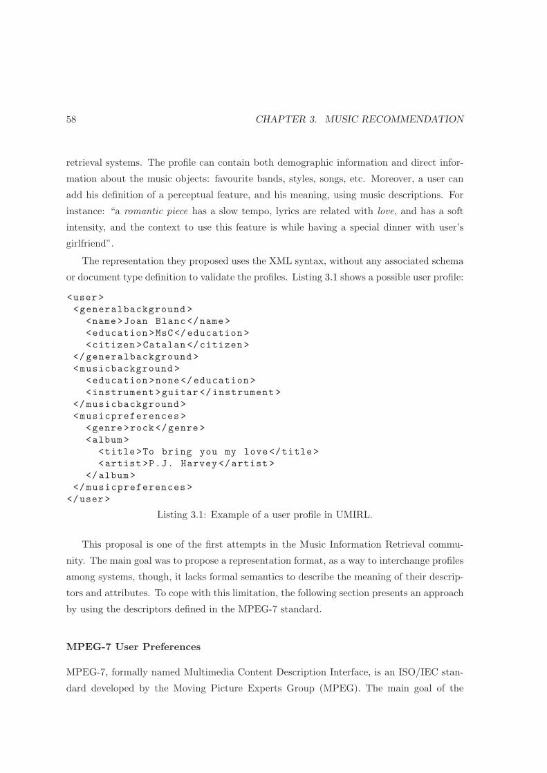
58 CHAPTER 3. MUSIC RECOMMENDATION
retrieval systems. The profile can contain both demographic information and direct infor-
mation about the music objects: favourite bands, styles, songs, etc. Moreover, a user can
add his definition of a perceptual feature, and his meaning, using music descriptions. For
instance: “a romantic piece has a slow tempo, lyrics are related with love, and has a soft
intensity, and the context to use this feature is while having a special dinner with user’s
girlfriend”.
The representation they proposed uses the XML syntax, without any associated schema
or document type definition to validate the profiles. Listing 3.1 shows a possible user profile:
<user>
<generalbackground >
<name>Joan Blanc </name>
<education >MsC</education >
<citizen >Catalan </citizen >
</generalbackground >
<musicbackground >
<education >none</education >
<instrument >guitar </instrument >
</musicbackground >
<musicpreferences >
<genre >rock</genre >
<album >
<title >To bring you my love</title >
<artist >P.J. Harvey </artist >
</album >
</musicpreferences >
</user>
Listing 3.1: Example of a user profile in UMIRL.
This proposal is one of the first attempts in the Music Information Retrieval commu-
nity. The main goal was to propose a representation format, as a way to interchange profiles
among systems, though, it lacks formal semantics to describe the meaning of their descrip-
tors and attributes. To cope with this limitation, the following section presents an approach
by using the descriptors defined in the MPEG-7 standard.
MPEG-7 User Preferences
MPEG-7, formally named Multimedia Content Description Interface, is an ISO/IEC stan-
dard developed by the Moving Picture Experts Group (MPEG). The main goal of the
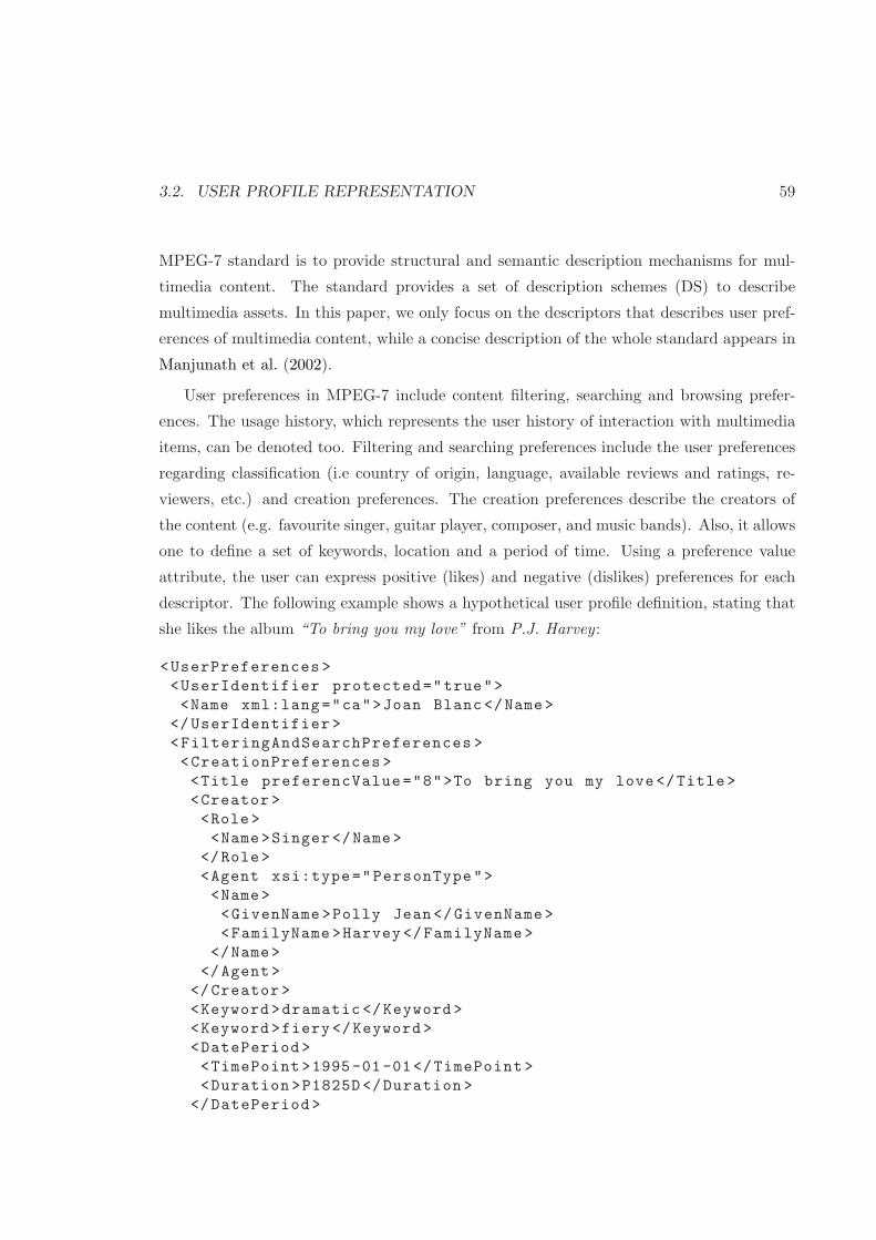
3.2. USER PROFILE REPRESENTATION 59
MPEG-7 standard is to provide structural and semantic description mechanisms for mul-
timedia content. The standard provides a set of description schemes (DS) to describe
multimedia assets. In this paper, we only focus on the descriptors that describes user pref-
erences of multimedia content, while a concise description of the whole standard appears in
Manjunath et al. (2002).
User preferences in MPEG-7 include content filtering, searching and browsing prefer-
ences. The usage history, which represents the user history of interaction with multimedia
items, can be denoted too. Filtering and searching preferences include the user preferences
regarding classification (i.e country of origin, language, available reviews and ratings, re-
viewers, etc.) and creation preferences. The creation preferences describe the creators of
the content (e.g. favourite singer, guitar player, composer, and music bands). Also, it allows
one to define a set of keywords, location and a period of time. Using a preference value
attribute, the user can express positive (likes) and negative (dislikes) preferences for each
descriptor. The following example shows a hypothetical user profile definition, stating that
she likes the album “To bring you my love” from P.J. Harvey :
<UserPreferences >
<UserIdentifier protected="true">
<Name xml:lang="ca">Joan Blanc </Name>
</UserIdentifier >
<FilteringAndSearchPreferences >
<CreationPreferences >
<Title preferencValue="8">To bring you my love</Title >
<Creator >
<Role>
<Name>Singer </Name>
</Role>
<Agent xsi:type="PersonType">
<Name>
<GivenName >Polly Jean</GivenName >
<FamilyName >Harvey </FamilyName >
</Name>
</Agent >
</Creator >
<Keyword >dramatic </Keyword >
<Keyword >fiery </Keyword >
<DatePeriod >
<TimePoint >1995 -01 -01</TimePoint >
<Duration >P1825D </Duration >
</DatePeriod >
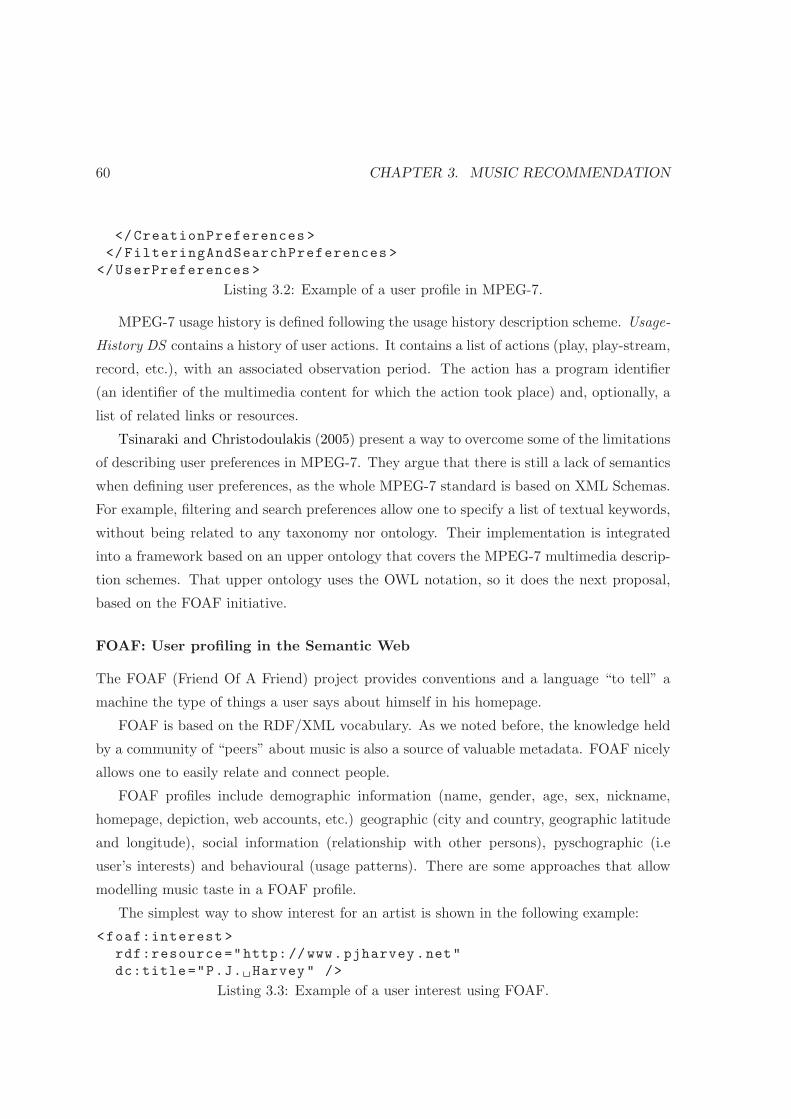
60 CHAPTER 3. MUSIC RECOMMENDATION
</CreationPreferences >
</FilteringAndSearchPreferences >
</UserPreferences >
Listing 3.2: Example of a user profile in MPEG-7.
MPEG-7 usage history is defined following the usage history description scheme. Usage-
History DS contains a history of user actions. It contains a list of actions (play, play-stream,
record, etc.), with an associated observation period. The action has a program identifier
(an identifier of the multimedia content for which the action took place) and, optionally, a
list of related links or resources.
Tsinaraki and Christodoulakis (2005) present a way to overcome some of the limitations
of describing user preferences in MPEG-7. They argue that there is still a lack of semantics
when defining user preferences, as the whole MPEG-7 standard is based on XML Schemas.
For example, filtering and search preferences allow one to specify a list of textual keywords,
without being related to any taxonomy nor ontology. Their implementation is integrated
into a framework based on an upper ontology that covers the MPEG-7 multimedia descrip-
tion schemes. That upper ontology uses the OWL notation, so it does the next proposal,
based on the FOAF initiative.
FOAF: User profiling in the Semantic Web
The FOAF (Friend Of A Friend) project provides conventions and a language “to tell” a
machine the type of things a user says about himself in his homepage.
FOAF is based on the RDF/XML vocabulary. As we noted before, the knowledge held
by a community of “peers” about music is also a source of valuable metadata. FOAF nicely
allows one to easily relate and connect people.
FOAF profiles include demographic information (name, gender, age, sex, nickname,
homepage, depiction, web accounts, etc.) geographic (city and country, geographic latitude
and longitude), social information (relationship with other persons), pyschographic (i.e
user’s interests) and behavioural (usage patterns). There are some approaches that allow
modelling music taste in a FOAF profile.
The simplest way to show interest for an artist is shown in the following example:
<foaf:interest >
rdf:resource="http: //www.pjharvey.net"
dc:title="P.J. Harvey" />
Listing 3.3: Example of a user interest using FOAF.
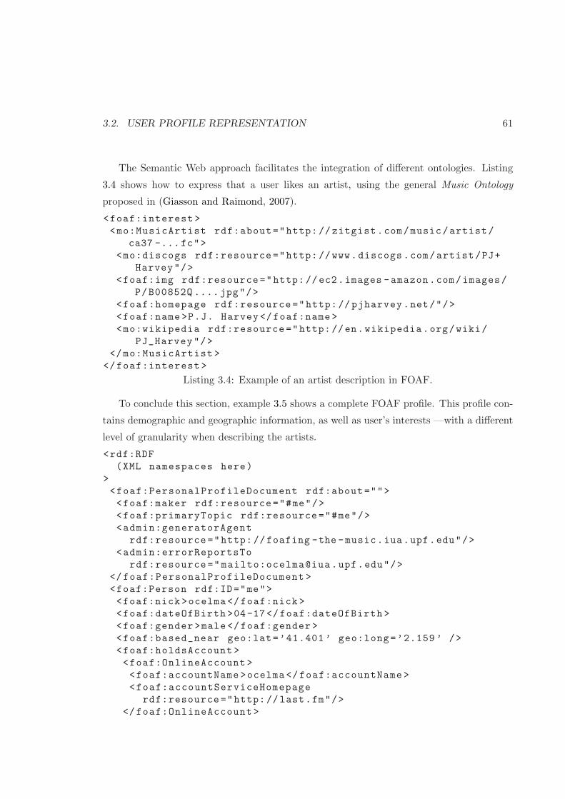
3.2. USER PROFILE REPRESENTATION 61
The Semantic Web approach facilitates the integration of different ontologies. Listing
3.4 shows how to express that a user likes an artist, using the general Music Ontology
proposed in (Giasson and Raimond, 2007).
<foaf:interest >
<mo:MusicArtist rdf:about="http: // zitgist.com/music/artist/
ca37 -...fc">
<mo:discogs rdf:resource="http: //www.discogs.com/artist/PJ+
Harvey"/>
<foaf:img rdf:resource="http: //ec2.images -amazon.com/images/
P/B00852Q .... jpg"/>
<foaf:homepage rdf:resource="http: // pjharvey.net/"/>
<foaf:name >P.J. Harvey </foaf:name >
<mo:wikipedia rdf:resource="http: //en.wikipedia.org/wiki/
PJ_Harvey"/>
</mo:MusicArtist >
</foaf:interest >
Listing 3.4: Example of an artist description in FOAF.
To conclude this section, example 3.5 shows a complete FOAF profile. This profile con-
tains demographic and geographic information, as well as user’s interests —with a different
level of granularity when describing the artists.
<rdf:RDF
(XML namespaces here)
>
<foaf:PersonalProfileDocument rdf:about="">
<foaf:maker rdf:resource="#me"/>
<foaf:primaryTopic rdf:resource="#me"/>
<admin:generatorAgent
rdf:resource="http: //foafing -the -music.iua.upf.edu"/>
<admin:errorReportsTo
rdf:resource="mailto:ocelma@iua .upf.edu"/>
</foaf:PersonalProfileDocument >
<foaf:Person rdf:ID="me">
<foaf:nick >ocelma </foaf:nick >
<foaf:dateOfBirth >04-17</foaf:dateOfBirth >
<foaf:gender >male</foaf:gender >
<foaf:based_near geo:lat=’41.401 ’ geo:long=’2.159 ’ />
<foaf:holdsAccount >
<foaf:OnlineAccount >
<foaf:accountName >ocelma </foaf:accountName >
<foaf:accountServiceHomepage
rdf:resource="http: //last.fm"/>
</foaf:OnlineAccount >
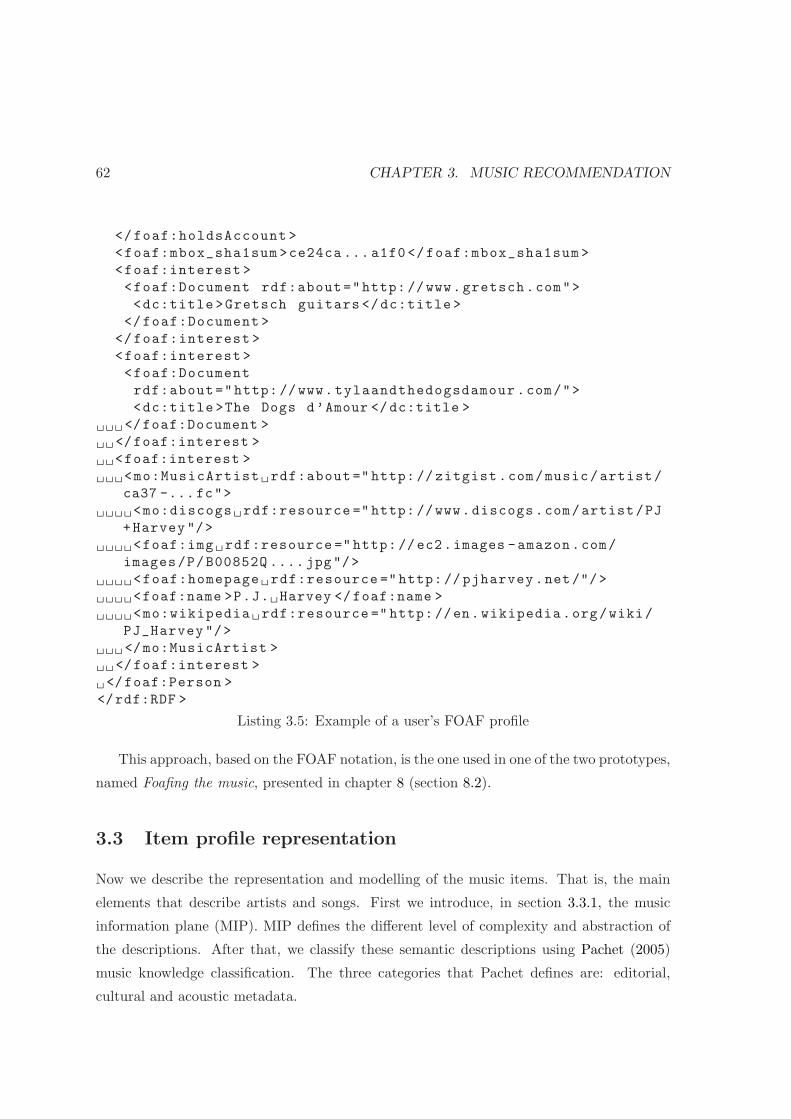
62 CHAPTER 3. MUSIC RECOMMENDATION
</foaf:holdsAccount >
<foaf:mbox_sha1sum >ce24ca ... a1f0</foaf:mbox_sha1sum >
<foaf:interest >
<foaf:Document rdf:about="http: //www.gretsch.com">
<dc:title >Gretsch guitars </dc:title >
</foaf:Document >
</foaf:interest >
<foaf:interest >
<foaf:Document
rdf:about="http: //www.tylaandthedogsdamour .com/">
<dc:title >The Dogs d’Amour </dc:title >
</foaf:Document >
</foaf:interest >
<foaf:interest >
<mo:MusicArtist rdf:about ="http: // zitgist.com/music/artist/
ca37 -...fc">
<mo:discogs rdf:resource ="http: //www.discogs.com/artist/PJ
+Harvey"/>
<foaf:img rdf:resource =" http: //ec2.images -amazon.com/
images/P/B00852Q .... jpg"/>
<foaf:homepage rdf:resource ="http: // pjharvey.net/"/>
<foaf:name >P.J. Harvey </foaf:name >
<mo:wikipedia rdf:resource ="http: //en.wikipedia.org/wiki/
PJ_Harvey"/>
</mo:MusicArtist >
</foaf:interest >
</foaf:Person >
</rdf:RDF >
Listing 3.5: Example of a user’s FOAF profile
This approach, based on the FOAF notation, is the one used in one of the two prototypes,
named Foafing the music, presented in chapter 8 (section 8.2).
3.3 Item profile representation
Now we describe the representation and modelling of the music items. That is, the main
elements that describe artists and songs. First we introduce, in section 3.3.1, the music
information plane (MIP). MIP defines the different level of complexity and abstraction of
the descriptions. After that, we classify these semantic descriptions using Pachet (2005)
music knowledge classification. The three categories that Pachet defines are: editorial,
cultural and acoustic metadata.

3.3. ITEM PROFILE REPRESENTATION 63
3.3.1 The music information plane
In the last twenty years, the signal processing and computer music communities have de-
veloped a wealth of techniques and technologies to describe audio and music content at the
lowest (or close–to–signal) level of representation. However, the gap between these low–level
descriptors and the concepts that music listeners use to relate with music collections (the
so–called “semantic gap”) is still, to a large extent, waiting to be bridged.
Due to the inherent complexity needed to describe multimedia objects, a layered ap-
proach with different levels of granularity is needed. In the multimedia field and, specially,
in the music field we foresee three levels of abstraction: low–level basic features, mid–level
semantic features, and high–level human understanding. The first level includes physical
features of the objects, such as the sampling rate of an audio file, as well as some basic
features like the spectral centroid of an audio frame, or even the predominant chord in a
sequential list of frames. A high–level of abstraction aims at describing concepts such as a
guitar solo, or tonality information (e.g key and mode) of a track. Finally, the higher level
should use reasoning methods and semantic rules to retrieve, for instance, several audio files
with “similar” guitar solos over the same key.
We describe the music information plane in two dimensions. One dimension considers
the different media types that serve as input data (audio, text and image). The other
dimension is the level of abstraction in the information extraction process of this data.
Figure 3.2 depicts the music information plane.
The input media types, in the horizontal axis, include data coming from: audio (music
recordings), text (lyrics, editorial text, press releases, etc.) and image (video clips, CD
covers, printed scores, etc.). On the other side, for each media type there are different levels
of information extraction (in the vertical axis). The lowest level is located at the signal
features. This level lays far away from what an end–user might find meaningful. Anyway, it
is the basis that allow to describe the content and to produce more elaborated descriptions
of the media objects. This level includes basic audio features (such as: energy, frequency,
mel frequency cepstral coefficients, or even the predominant chord in a sequential list of
frames), or basic natural language processing for the text media. At the mid–level (the
content objects level), the information extraction process and the elements described are a
bit closer to the end–user. This level includes description of musical concepts (such as a
guitar solo, or tonality information —e.g key and mode— of a music title), or named entity
recognition for text information. Finally, the higher–level, the human knowledge, includes

64 CHAPTER 3. MUSIC RECOMMENDATION
Figure 3.2: The music information plane. The horizontal axis includes the input mediatypes. The vertical axis represents the different levels of information extraction for eachmedia type. At the top, a user interacts with the music content and the social network ofusers.
information related with the human beings when interacting with music knowledge. This
level could use inference methods and semantic rules to retrieve, for instance, several audio
files with similar guitar solos over the same key. At the highest level, there is the user, and
the social relationships with a community of users. Figure 3.2 depicts the music information
plane.
Nonetheless, the existing semantic gap between concept objects and human knowledge
invalidates any possible direct assignment of music descriptors to users. This has many

3.3. ITEM PROFILE REPRESENTATION 65
consequences to music understanding and music recommendation. Yet, there are some
open questions, such as: what are the music elements that makes a person feel certain
emotions, or to evoke some particular memories? How is a personal identity linked with
music? Only a multi–modal approach, that takes into account as much elements from MIP
as possible, would be able to (partly) answer some of these questions. Furthermore, we
argue that user intervention is important for adding semantics to music understanding.
That said, we believe that neither pure bottom–up nor top–down approaches can lead to
bridge this gap. We foresee, then, an approximation in both ways: users need to interact
with the content to add proper (informal) semantics (e.g. via tagging), and also content
object descriptions must be somehow understandable by the users.
Pachet (2005) classifies the music knowledge management in three categories. This
classification allows one to create meaningful descriptions of music, and to exploit these
descriptions to build music recommendation systems. The three categories that Pachet
defines are: editorial, cultural and acoustic metadata. We include this classification as an
orthogonal axis that lays over the music information plane.
3.3.2 Editorial metadata
Editorial metadata (EM) consists of information manually entered by an editor. Usually,
the information is decided by an expert, or a group of experts. Figure 3.3 depicts the
relationship between editorial metadata and the music information plane.
EM includes simple creation and production information (e.g. the song C’mon Billy,
written by P.J. Harvey in 1995, was produced by John Parish and Flood, and the song
appears as the track number 4, on the album “To bring you my love”). EM includes, in
addition, artist biography, genre information, relationships among artists, etc. As it can be
seen, editorial information is not necessarily objective. It is usual the case that different
experts cannot agree in assigning a concrete genre to a song or to an artist. Even more
difficult is a common consensus of a taxonomy of musical genres.
The scope of EM is rather broad. Yet, it usually refers to these items: the creator
(or author) of the content, the content itself, and the structure of the content. Regarding
the latter, editorial metadata can be fairly complex. For example, an opera performance
description has to include the structure of the opera. It is divided in several acts. Each
act has some scenes. In a given scene, there is a soprano singing an Aria piece, and many
musicians playing. It has lyrics to sing, and these can be in different languages (sung in
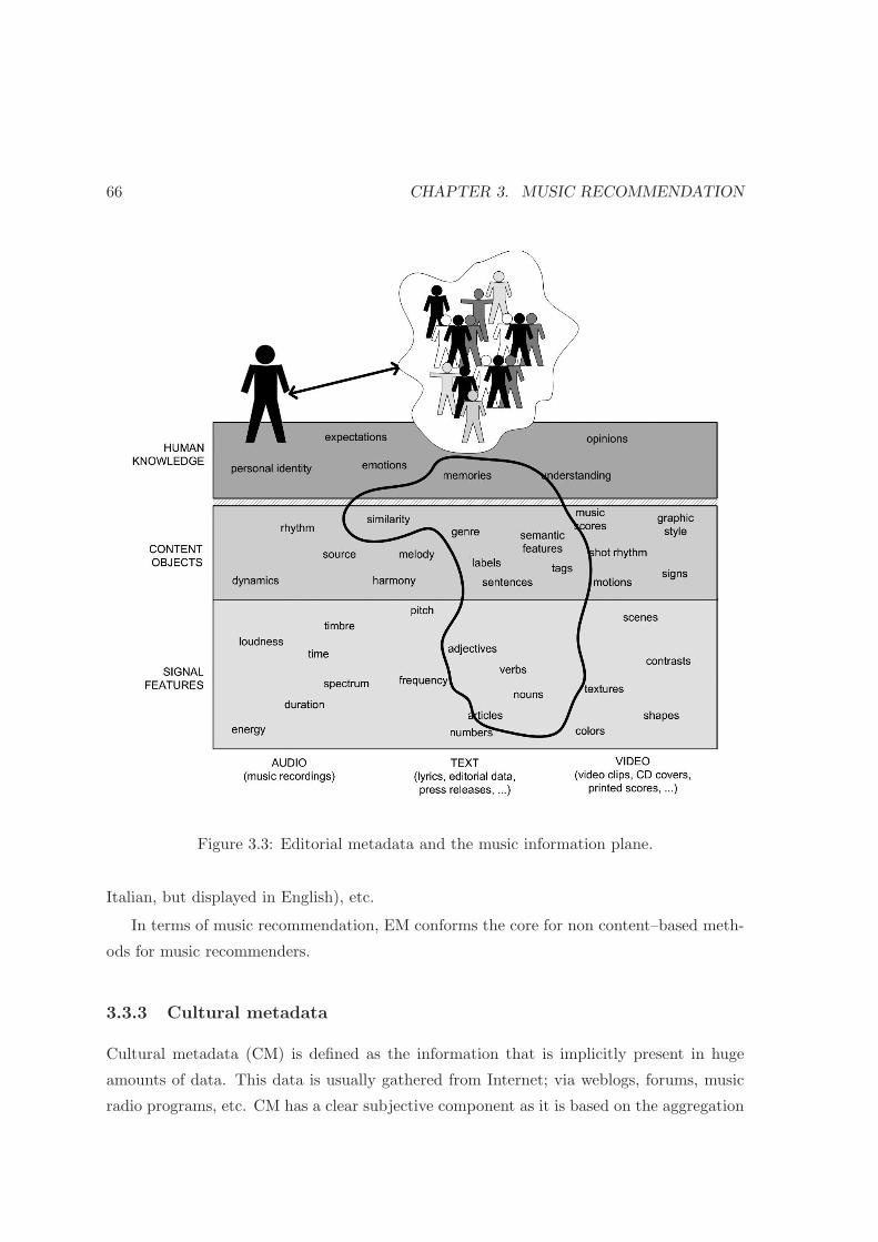
66 CHAPTER 3. MUSIC RECOMMENDATION
Figure 3.3: Editorial metadata and the music information plane.
Italian, but displayed in English), etc.
In terms of music recommendation, EM conforms the core for non content–based meth-
ods for music recommenders.
3.3.3 Cultural metadata
Cultural metadata (CM) is defined as the information that is implicitly present in huge
amounts of data. This data is usually gathered from Internet; via weblogs, forums, music
radio programs, etc. CM has a clear subjective component as it is based on the aggregation

3.3. ITEM PROFILE REPRESENTATION 67
Figure 3.4: Cultural metadata and the music information plane.
of personal opinions. Figure 3.4 depicts the relationship between cultural metadata and the
music information plane.
Turnbull et al. (2008) present five different ways to collect annotations at artist (or song)
level. The approaches are:
• mining web documents,
• harvesting social tags,
• autotagging audio content,

68 CHAPTER 3. MUSIC RECOMMENDATION
• deploying annotation games, and
• conducting a survey
In the following section we describe web document mining. Autotagging is briefly men-
tioned in section 3.3.4.
Web–MIR techniques to describe artists
Web Music Information Retrieval (Web–MIR) is a recent field of research in the MIR
community. Web–MIR focuses on the analysis and exploitation of cultural information.
So far, performances close to classic content–based approaches, are reported on artist
genre classification, and artist similarity (Whitman and Lawrence, 2002; Schedl et al., 2008;
Knees et al., 2008). Yet, it is not clear how Web–MIR methods can deal with long tail con-
tent.
The origins of Web–MIR can be found in the earlier work of Whitman and Lawrence
(2002); Whitman (2003). They describe artists using a list of weighted terms. To gather
artist related terms, they query a general search engine with the name of the artist. To
limit the size of the page results, they add some keywords to the query, such as “music”
and “review”. From the retrieved pages, the authors extract unigrams, bigrams and noun
phrases. Whitman (2003) uses an unsupervised method for music understanding, using the
power spectral density estimate (PSD) over each 5 seconds of audio. Then, it keeps the
semantically dimensions that contain the most significant meanings.
Similarly, Baumann and Hummel (2005) improved this approach by filtering irrelevant
content of the web pages (e.g. adverts, menus, etc.). The description of an artist is con-
formed by the terms with the highest normalised TF/IDF value. That includes the most
relevant nouns, adjectives and simple phrases, as well as un–tagged unigrams and bigrams.
In Geleijnse and Korst (2006), the authors present different ways to describe artists
using web data, based on co–occurrences analysis between an artist and the labels used. The
set of labels are previously defined, and conform a corpus of music related terms (e.g. genres,
instruments, moods, etc.). The three methods they use are: Pagecount–based mapping
(PCM), Pattern–based mapping (PM), and Document–based mapping (DM). PCM uses the
total number of hits retrieved by Google search engine. However, some terms appear more
often than others (e.g. pop, or rock versus cumbia). So, they provide a normalised version,
inspired by Pointwise mutual information (see section 2.5.4). Pattern–based mapping uses
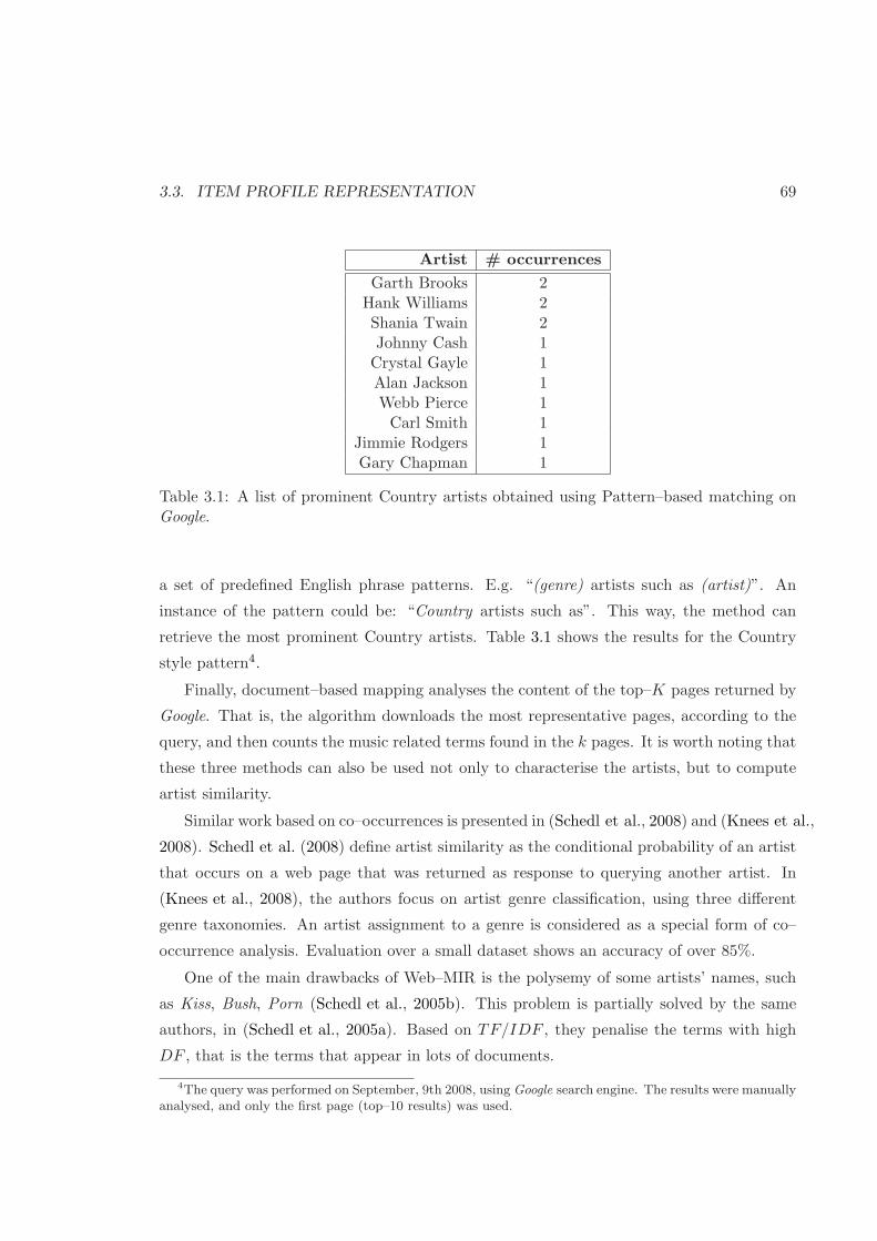
3.3. ITEM PROFILE REPRESENTATION 69
Artist # occurrences
Garth Brooks 2Hank Williams 2Shania Twain 2Johnny Cash 1
Crystal Gayle 1Alan Jackson 1Webb Pierce 1
Carl Smith 1Jimmie Rodgers 1Gary Chapman 1
Table 3.1: A list of prominent Country artists obtained using Pattern–based matching onGoogle.
a set of predefined English phrase patterns. E.g. “(genre) artists such as (artist)”. An
instance of the pattern could be: “Country artists such as”. This way, the method can
retrieve the most prominent Country artists. Table 3.1 shows the results for the Country
style pattern4.
Finally, document–based mapping analyses the content of the top–K pages returned by
Google. That is, the algorithm downloads the most representative pages, according to the
query, and then counts the music related terms found in the k pages. It is worth noting that
these three methods can also be used not only to characterise the artists, but to compute
artist similarity.
Similar work based on co–occurrences is presented in (Schedl et al., 2008) and (Knees et al.,
2008). Schedl et al. (2008) define artist similarity as the conditional probability of an artist
that occurs on a web page that was returned as response to querying another artist. In
(Knees et al., 2008), the authors focus on artist genre classification, using three different
genre taxonomies. An artist assignment to a genre is considered as a special form of co–
occurrence analysis. Evaluation over a small dataset shows an accuracy of over 85%.
One of the main drawbacks of Web–MIR is the polysemy of some artists’ names, such
as Kiss, Bush, Porn (Schedl et al., 2005b). This problem is partially solved by the same
authors, in (Schedl et al., 2005a). Based on TF/IDF , they penalise the terms with high
DF , that is the terms that appear in lots of documents.
4The query was performed on September, 9th 2008, using Google search engine. The results were manuallyanalysed, and only the first page (top–10 results) was used.

70 CHAPTER 3. MUSIC RECOMMENDATION
Another common drawback of all the previous approaches is the high dimensional-
ity of the datasets. To avoid this problem, Pohle et al. (2007) use Non–negative Matrix
Factorisation to reduce the dimensionality of the artist–term matrix. They also use a
predefined vocabulary of music terms, and analyse the content of the top–100 web pages
related to each artist. To get the most relevant pages, they use a similar approach as
(Whitman and Lawrence, 2002). The original matrix contains all the terms applied to the
artists, using TF/IDF weights. This matrix is decomposed into 16 factors, or “archetyp-
ical” concepts using non–negative matrix factorisation. Then, each artist is described by
a 16–dimensional vector. After that, a music browser application allows users to navigate
the collection by adjusting the weights of the derived concepts, and also can recommend
similar artists using cosine distance over the artists’ vectors.
Finally, Pachet et al. (2001) compute artist and song co–occurrences from radio sources,
and also from a big database of CD compilations, extracted from CDDB. Zadel and Fujinaga
(2004) investigate artist similarity using Amazon and Listmania! APIs, and then Google
to refine the results, using artist co–occurrences in webpages.
Collecting ground truth data
An important aspect when trying to evaluate similarity metrics using cultural metadata is
the creation of reliable ground truth data. Different proposals are presented in (Ellis et al.,
2002), (Baumann and Hummel, 2005), (Pachet, 2005) and (Geleijnse et al., 2007). The
problem of gathering ground–truth for music similarity evaluation is outlined in Berenzweig et al.
(2003). The most recent proposal, by Geleijnse et al. (2007), focus on creating a dynamic
ground truth for artist tagging and artist similarity. The idea is to adapt to the dynamically
changing data being harvested by social tagging (e.g. from last.fm), instead of defining a
static and immutable ground truth.
Cultural information, based on Web–MIR and social tagging techniques, is the basis
for context–based music recommenders. Section 3.4.3 presents the main ideas to exploit
cultural information, and use it to provide music recommendations.
3.3.4 Acoustic metadata
The last category of semantic music description is acoustic metadata. Acoustic metadata
is obtained using content analysis of an audio file. Semantic acoustic descriptors are the
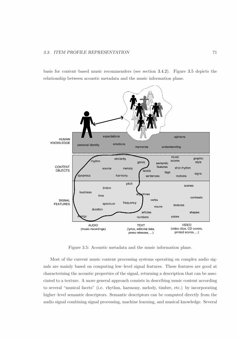
3.3. ITEM PROFILE REPRESENTATION 71
basis for content–based music recommenders (see section 3.4.2). Figure 3.5 depicts the
relationship between acoustic metadata and the music information plane.
Figure 3.5: Acoustic metadata and the music information plane.
Most of the current music content processing systems operating on complex audio sig-
nals are mainly based on computing low–level signal features. These features are good at
characterising the acoustic properties of the signal, returning a description that can be asso-
ciated to a texture. A more general approach consists in describing music content according
to several “musical facets” (i.e. rhythm, harmony, melody, timbre, etc.) by incorporating
higher–level semantic descriptors. Semantic descriptors can be computed directly from the
audio signal combining signal processing, machine learning, and musical knowledge. Several
72 CHAPTER 3. MUSIC RECOMMENDATION
of the shortcomings of the purely data driven techniques can be overcome by applying mu-
sical knowledge, and this musical knowledge should not be exclusive for musically trained
people. The following sections are devoted to outlining some relevant music description
facets.
Timbre and instrumentation
Extracting truly instrumental information from music, as pertaining to separate instru-
ments or types of instrumentation implies classifying, characterising and describing infor-
mation which is buried behind many layers of highly correlated data. Given that the
current technologies do not allow a sufficiently reliable separation, work has concentrated
on the characterisation of the “overall” timbre or “texture” of a piece of music as a func-
tion of low–level signal features. This approach implied describing mostly the acousti-
cal features of a given recording, gaining little knowledge about its instrumental contents
(Aucouturier and Pachet, 2004).
Even though it is not possible to separate the different contributions and “lines” of the
instruments, there are some simplifications that can provide useful descriptors (e.g. lead
instrument recognition, solo detection). The recognition of idiosyncratic instruments, such
as percussive ones, is another valuable simplification. Given that the presence, amount
and type of percussion instruments are very distinctive features of some music genres
and, hence, can be exploited to provide other natural partitions to large music collections.
(Herrera et al., 2004) have defined semantic descriptors such as the percussion index or the
percussion profile. Although they can be computed after some source separation, reasonable
approximations can be achieved using simpler sound classification approaches that do not
attempt separation (Yoshii et al., 2004).
Additionally, Chetry et al. (2005) contributed to the current state of the art in instru-
ment identification of mono–instrumental music, using line spectral frequencies (LSF) and
a k–means classifier (Herrera et al., 2006).
Rhythm
In its most generic sense, rhythm refers to all of the temporal aspects of a musical work,
whether represented in a score, measured from a performance, or existing only in the percep-
tion of the listener (Gouyon and Dixon, 2005). In the literature the concept of “automatic
rhythm description” groups many applications as diverse as tempo induction, beat tracking,

3.3. ITEM PROFILE REPRESENTATION 73
rhythm quantisation, meter induction and characterisation of timing deviations, to name
a few. Many of these different aspects have been investigated, from the low–level onset
detection, to the characterisation of music according to rhythmic patterns.
At the core of automatic rhythmic analysis lies the issue of identifying the start, or
onset time, of events in the musical data. As an alternative to standard energy–based ap-
proaches, another methodologies have recently appeared: a method that works solely with
phase information (Bello and Sandler, 2003), or that are based on predicting the phase and
energy of signal components in the complex domain (Bello et al., 2004), greatly improving
results for both percussive and tonal onsets. However, there is more to rhythm than the
absolute timings of successive musical events. For instance, Davies and Plumbley (2004)
have proposed a general model to beat tracking, based on the use of comb–filtering tech-
niques on a continuous representation of “onset emphasis”, i.e. an onset detection function.
Subsequently, the method was expanded to combine this general model with a context–
dependent model by including a state space switching model. This improvement has been
shown to significantly improve upon previous results, in particular with respect to main-
taining a consistent metrical level and preventing phase switching between off–beats and
on–beats.
Furthermore, the work done by Gouyon and Dixon (2004) and Dixon et al. (2004) demon-
strates the use of high–level rhythmic descriptors for genre classification of recorded audio.
An example is a tempo–based classification showing the high relevance of this feature while
trying to characterise dance music (Gouyon and Dixon, 2004). However, this approach is
limited by the assumption that, given a musical genre, the tempo of any instance is among a
very limited set of possible tempi. To address this, Dixon et al. (2004) use bar–length rhyth-
mic patterns for the classification of dance music. The method dynamically estimates the
characteristic rhythmic pattern on a given musical piece, by a combination of beat tracking,
meter annotation and a k–means classifier. Genre classification results are greatly improved
by using these high–level descriptors, showing the relevance of musically–meaningful repre-
sentations for Music Information Retrieval (MIR) tasks. Finally, a holistic approach toward
automated beat tracking, taking into account music structure is presented in (Dannenberg,
2005).

74 CHAPTER 3. MUSIC RECOMMENDATION
Harmony
The harmony of a piece of music can be defined by the combination of simultaneous notes, or
chords; the arrangement of these chords along time, in progressions; and their distribution,
which is closely related to the key or tonality of the piece. Chords, their progressions, and
the key are relevant aspects of music perception that can be used to accurately describe
and classify music content.
Harmonic based retrieval has not been extensively explored before. A successful ap-
proach at identifying harmonic similarities between audio and symbolic data was presented
in (Pickens et al., 2002). It relied on automatic transcription, a process that is partially
effective within a highly constrained subset of musical recordings (e.g. mono–timbral, no
drums or vocals, small polyphonies). To avoid such constraints (Gomez, 2006b) adopts the
approach where describes the harmony of the piece, without attempting to estimate the
pitch of notes in the mixture. Avoiding the transcription step allows to operate on a wide
variety of music. This approach requires the use of a feature set that is able to empha-
sise the harmonic content of the piece, such that this representation can be exploited for
further, higher–level, analysis. The feature set of choice is known as a Chroma or Pitch
Class Profile, and they represent the relative intensity of each of the twelve semitones of
the equal–tempered scale.
Gomez and Herrera (2004) presents the tonality estimation by correlating chroma distri-
butions with key profiles derived from music cognition studies. Results show high recogni-
tion rates for a database of recorded classical music. The studies done in (Harte and Sandler,
2005) have also concentrated on chord estimation based on chroma features, using tuning,
and a simple template–based model of chords. Recognition rates of over 66% were found for
a database of recorded classical music, though the algorithm is being used also with other
musical genres. A recent development includes the generation of a harmonic representation
using a Hidden Markov Model, initialised and trained using musical theoretical and cogni-
tive considerations (Bello and Pickens, 2005). This methodology has already shown great
promise for both chord recognition and structural segmentation.
For a complete and deeper overview of all these techniques, the reader is referred to
(Gomez, 2006a).

3.3. ITEM PROFILE REPRESENTATION 75
Intensity
Subjective intensity, or the sensation of energeticness we get from music, is a concept com-
monly and easily used to describe music content. Although intensity has a clear subjective
facet, Sandvold et al. hypothesised that it could be grounded on automatically extracted
audio descriptors. Inspired by the findings of Zils and Pachet (2003), Sandvold and Herrera
(2004) created a model of subjective intensity built from energy and timbre low–level de-
scriptors extracted from the audio data. They have proposed a model that decides among
5 labels (ethereal, soft, moderate, energetic, and wild), with an estimated effectiveness of
nearly 80%. The model has been developed and tested using several thousands of subjective
judgements.
Structure
Music structure refers to the ways music materials are presented, repeated, varied or con-
fronted along a piece of music. Strategies for doing that are artist, genre and style–specific
(i.e. the A–B themes exposition, development and recapitulation of a sonata form, or the
intro–verse–chorus–verse–chorus–outro of “pop music”). Detecting the different structural
sections, the most repetitive segments, or even the least repeated segments, provide power-
ful ways of interacting with audio content based on summaries, fast–listening and musical
gist–conveying devices, and on–the–fly identification of songs.
The section segmenter developed by Ong and Herrera (2005) extracts segments that
roughly correspond to the usual sections of a pop song or, in general, to sections that are
different (in terms of timbre and tonal structure) from the adjacent ones. The algorithm
first performs a rough segmentation with the help of change detectors, morphological filters
adapted from image analysis, and similarity measurements using low–level descriptors. It
then refines the segment boundaries using a different set of low–level descriptors. Com-
plementing this type of segmentation, the most repetitive musical pattern in a music file
can also be determined by looking at self–similarity matrices in combination with a rich set
of descriptors including timbre and tonality (i.e. harmony) information (Ong and Herrera,
2005). Ground–truth databases for evaluating this task are still under construction, but
first evaluations yielded an effectiveness of section boundary detection higher than 70%.
76 CHAPTER 3. MUSIC RECOMMENDATION
3.4 Recommendation methods
In this section, we present the music recommendation methods to match user preferences
(see section 3.2) with the item descriptions (presented in section 3.3).
3.4.1 Collaborative filtering
Collaborative filtering (CF) techniques have been largely applied in the music domain. CF
makes use of the editorial and cultural information. Early research was based on explicit
feedback, based on the ratings about songs or artists. Yet, tracking user listening habits
has become the most common way in music recommendation. In this sense, CF has to deal
with implicit feedback (instead of explicit ratings).
Explicit feedback
Ringo, described in (Shardanand, 1994), is the first music recommender based on collab-
orative filtering and explicit feedback. The author applies user–based CF approach (see
section 2.5.2). Similarity among users is computed with Pearson normalised correlation
(see Equation 2.4). Then, the recommendations are computed as the mean of the ratings
done by the similar users of the active user (see Equation 2.1).
Racofi (Rule Applying COllaborative FIltering) Music combines collaborative filtering
based on ratings, and a set of logic rules based on Horn clauses (Anderson et al., 2003).
The rules are applied after the ratings have been gathered. The five rating dimensions they
define are: impression, lyrics, music, originality, and production. The objective of the rules
is to prune the output of the collaborative filtering, and promote the items that the user
will be most familiar with. Anderson et al. (2003) exemplifies a rule:
“If a user rates 9 the originality of an album by artist X then the predicted
originality rating, for this user, of all other albums by artist X is increased by a
value of 0.5”.
These kind of rules implicitly modify the ratings that a user has done previously. The
Indiscover music recommender system5 implements this approach.
5http://www.indiscover.net
3.4. RECOMMENDATION METHODS 77
Implicit feedback
Implicit feedback in the music domain is usually gathered from the listening habits. The
main drawback is that the value that a user assigns to an item is not in a predefined
range (e.g. from 1..5 or like it/hate it). Instead, the interaction between users and items is
described by the total playcounts. Thus, the system can only track positive feedback (i.e.
tracks that a user listens to). Implicit negative feedback cannot be gathered. When users
explicitly rate the content, the range of values include both positive and negative feedback
(e.g. from 1..5, where 1 means a user does not like the item, 3 indifference, and 5 she loves
the item).
Furthermore, recommendations are usually performed at artist level, but the listening
habits are at song level. In this case, an aggregation process, from song plays to artist total
playcounts, is needed.
To use CF with implicit feedback at artist level, there are different options:
• Convert the implicit data into a binary user–artist matrix. Non–zero cells mean that
the user has listened to the artist at least once.
• Transform the implicit data into a normalised matrix. Instead of assigning 0/1 to a
cell, the value can denote how much a user listens to the artist (e.g. [5..1], where
5 denotes that she listens to a lot the artist, and 1 mean only from time to time).
The matrix has a more fine–grained description of the user listening habits than the
previous, binary, normalisation.
• Normalise each row (users), so that the sum of the row entries equal 1. This option,
then, describes the artist probability distribution of a user.
• Create a user–artist matrix with the total playcounts in the cells. In this case there
is no normalisation, as the matrix contains the absolute values.
In any case, after the dataset is represented in the user–artist matrix, one can apply the
CF methods with explicit feedback (presented in section 2.5.2).
We have done some experiments with data obtained from last.fm. The dataset con-
tains the listening habits for more than 500,000 users, and a total of around 30 million
〈user, artist, plays〉 triples. To clean the list of artists, we only use those artists that have a
Musicbrainz 6 ID, and that at least 10 users have listen to once or more. After the cleaning
process, we get a list of around 95,000 distinct artists. To apply CF, we transformed the
6http://www.musicbrainz.org
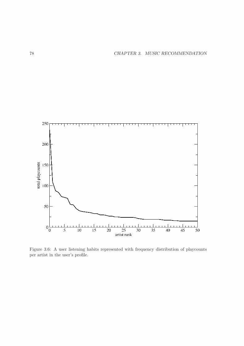
78 CHAPTER 3. MUSIC RECOMMENDATION
Figure 3.6: A user listening habits represented with frequency distribution of playcountsper artist in the user’s profile.
3.4. RECOMMENDATION METHODS 79
listening habits dataset to a user–artist matrix M . Mi,j represents the number of times
user i has listened to artist j. To normalise the matrix we followed the second approach,
that is to assign a range value [1..5] in Mi,j from the 〈useri, artistj , plays〉 data.
Usually, the user’s listening habits distribution is skewed to the right, so it shows a
heavy–tailed curve. That is, a few artists have lots of plays in the user profile, and the
rest of artists have much less playcounts. We compute the complementary cumulative
distribution of artist plays in the user profile. Artists locate in the top 80–100% of the
distribution get a score of 5, artists in the 60–80% range get a 4, and so on (until the artists
with less playcounts, in the 0–20% range, which get assigned a 1).
Figure 3.6 depicts the listening habits of a user in terms of total playcounts. The
horizontal axis contains her top–50 artists, ranked by the total plays (i.e. artist at position
1 has 238 playcounts). Figure 3.7 shows the complementary cumulative distribution of the
artist playcounts from Figure 3.6. This distribution is the one used to normalise the user
playcounts in the range of 5..1.
Sometimes, the listening habits distribution of a user is not skewed, but very homoge-
neous (a small standard deviation value, and a median close to the mean value). To detect
this type of distribution, we use the coefficient of variation, CV . CV is a normalised mea-
sure of dispersion of a probability distribution, that divides the standard deviation by the
mean value, CV = σµ . If CV ≤ 0.5 we do not use the complementary cumulative distribu-
tion. Instead, we assign a value of 3 to all the user artists, meaning that all the artists in
the profile have a similar number of plays.
Once the normalisation process is done, it is straightforward to compute the average
value of normalised plays for an artist, as well as for a user —in case that the item similarity
measure to use is either Pearson correlation (Equation 2.4) or adjusted cosine (Equation
2.3). The next step is to compute artist similarity using the user–artist M matrix that
contains the listening habits, normalised in the range of [1..5].
An example
Using matrix M , we present two concrete examples of item–simiarity using Pearson cor-
relation, and conditional probability (defined in Equation 2.5). Table 3.2 (left) shows the
top–10 similar artists of The Dogs d’Amour7, whilst the right column shows the results
obtained using conditional probability similarity.
7http://en.wikipedia.org/wiki/The_Dogs_D’Amour
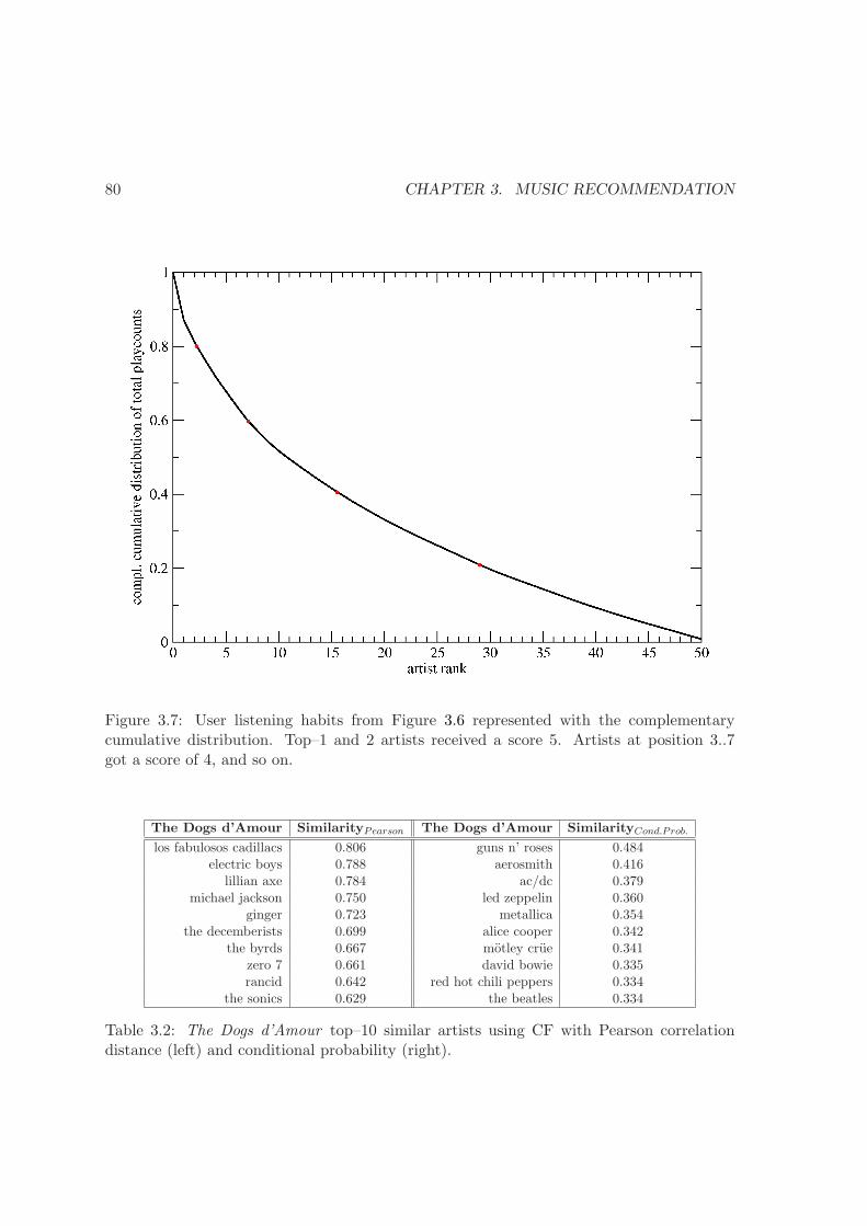
80 CHAPTER 3. MUSIC RECOMMENDATION
Figure 3.7: User listening habits from Figure 3.6 represented with the complementarycumulative distribution. Top–1 and 2 artists received a score 5. Artists at position 3..7got a score of 4, and so on.
The Dogs d’Amour SimilarityPearson The Dogs d’Amour SimilarityCond.Prob.
los fabulosos cadillacs 0.806 guns n’ roses 0.484electric boys 0.788 aerosmith 0.416
lillian axe 0.784 ac/dc 0.379michael jackson 0.750 led zeppelin 0.360
ginger 0.723 metallica 0.354the decemberists 0.699 alice cooper 0.342
the byrds 0.667 motley crue 0.341zero 7 0.661 david bowie 0.335rancid 0.642 red hot chili peppers 0.334
the sonics 0.629 the beatles 0.334
Table 3.2: The Dogs d’Amour top–10 similar artists using CF with Pearson correlationdistance (left) and conditional probability (right).

3.4. RECOMMENDATION METHODS 81
We can see that the asymmetric conditional probability metric is completely biased
towards popular artists, whilst Pearson similarity contains artists across the long tail, also
ranging different styles (including some unexpected results, such as Michael Jackson or
Zero 7 ). Top–10 similar artists list, obtained by conditional probability, contain some of
the most representative and prototypical artists of the seed artist’s main styles (that is,
glam, rock, and hard–rock). The similarity value using conditional probability is also quite
informative; 48.4% of the users who listen to The Dogs d’Amour also listen to Guns n’
Roses (but not the other way around!).
3.4.2 Content–based filtering
Recommender systems using content–based filtering are based on item–to–item similarity.
Audio content–based methods are used to rank music titles, based on audio similarity. Thus,
a recommender system has to compute the similarity among songs, and use this information
to recommend music. Artist similarity can also be computed, by agreggating song similarity
results. There are two orthogonal ways to annotate songs; automatically or manually. The
following sections present each approach.
Automatic feature extraction
Generally speaking, once the audio has been semantically annotated (see section 3.3), and
the similarity among the items has been computed, content–based filtering for a given user
is rather simple. It is based on presenting songs (or artists) that “sound” similar to the
user profile.
The first work related with music similarity focused on low–level descriptors, such as the
Mel Frequency Cepstral Coefficients (MFCC). These approaches aimed at deriving timbre
similarity, but have also been used to take on other problems, such as genre classifica-
tion. Foote proposed a music indexing system based on MFCC histograms (Foote, 1997).
Aucouturier and Pachet (2002) presented a Gaussian mixture model based on MFCC. They
also could generate playlists based on timbre similarity and some global constraints of the
output playlist. Similarity measures on top of the MFCC+GMM combination includes
Kullback–Leibler (KL) divergence, and the earth mover’s distance. KL divergence measures
the relative similarity between two single-Gaussian distributions of data. A small divergence
in the distributions means that the two songs are similar. Earth mover’s distance (EMD)
has been largely applied in the image community, to retrieve similar images. The adoption

82 CHAPTER 3. MUSIC RECOMMENDATION
in the music field was presented in Logan and Salomon (2001). Audio signatures can be
compared using the EMD, which allows comparison of histograms with disparate bins.
However, none of these methods capture information about long–term structure ele-
ments, such as the melody, ryhthm, or harmony. To cope with this limitation, Tzanetakis
(2002) extracted a set of features representing the spectrum, rhythm and harmony (chord
structure). All the features are merged into a single vector, and it is used to determine
similarity. For a complete overview on audio similarity, the reader is referred to (Pampalk,
2006).
Cataltepe (2007) presents a music recommendation system based on audio similarity
They also take into account the user’s listening history. The hypothesis is that users give
more importance to different aspects of music. These aspects can be described and classi-
fied using semantic audio features. Using this adaptative content–based recommendation
scheme, as opposed to a static set of features, resulted in up to 60% of increment in the
accuracy of the recommendations.
User’s relevance feedback for content–based music systems is presented in (Hoashi et al.,
2003). To reduce the burden of users to input learning data into the system, they propose
a method to generate user profiles based on genre preferences, and a posterior refinement
based on relevance feedback from the recommendations (Rocchio, 1971).
Manual feature extraction
Human–based annotation of music is very time consuming, but can be more accurate than
automatic feature extraction methods. Pandora’s approach is based on manual descriptions
of the audio content. Pandora’s web site explains their procedure8:
“(. . .) our team of thirty musician-analysts have been listening to music, one
song at a time, studying and collecting literally hundreds of musical details on
every song. It takes 20-30 minutes per song to capture all of the little details
that give each recording its magical sound —melody, harmony, instrumentation,
rhythm, vocals, lyrics . . . and more— close to 400 attributes! (. . .)”
The analysts have to annotate around 400 parameters per song, using a ten point scale
[0..10] per attribute. There is a clear scalability problem; time–constraints allow people
to add about 15,000 songs per month. Also, they have to deal with the variability across the
8http://www.pandora.com/corporate/index.shtml Last accessed date: September 10th, 2008
3.4. RECOMMENDATION METHODS 83
analysts. Cross validation is also needed in order to assure the quality (and avoid analysts’
bias) of the annotations.
Simple weighted Euclidean distance is used to find similar songs9. Song selection is, then,
based on nearest neighbors. However, they assign specific weights to important attributes,
such as genre. For artist similarity they only use specific songs, not an average of all
the artist’s songs. Pandora’s ultimate goal is to offer a mix of familiarity, diversity, and
discovery.
An example
Now we present an example of artist similarity derived from automatic audio feature extrac-
tion. To compute artist similarity, we apply content–based audio analysis in an in–house
music collection (T ) of 1.3 Million tracks of 30 seconds samples. Our audio analysis con-
siders not only timbral features (e.g. Mel frequency cepstral coefficients), but some musical
descriptors related to rhythm (e.g. beats per minute, binary/ternary metric), and tonality
(e.g chroma features, key and mode), among others (Cano et al., 2005). Then, to compute
artist similarity we used the most representative tracks, Ta, of an artist a, with a maximum
of 100 tracks per artist. For each track, ti ∈ Ta, we obtain the most similar tracks (excluding
those from artist a):
sim(ti) = argmin∀t∈T
(distance(ti, t)), (3.1)
and get the artists’ names, Asim(ti), of the similar tracks. The list of (top–20) similar artists
of a comes from Asim(ti), ranked by a combination of the artist frequency (how many songs
from the artist are similar to seed track ti), and the similarity distance:
similar artists(a) =⋃
Asim(ti),∀ti ∈ Ta (3.2)
Table 3.3 shows the top–20 similar artists for two seed artists, Aerosmith10 and Alejandro
Sanz 11. Regarding Aerosmith’s top–20 similar artists, most of the bands belong to the
same genre, that is classic hard rock. Yet, some bands belong to the punk/rock style (e.g.
NOFX, MxPx, New found glory, Slick shoes, and The Damned). These bands could still
9Personal communication with Pandora staff, during July 200710For more information about the artist see http://en.wikipedia.org/wiki/Aerosmith11For more information about the artist see http://en.wikipedia.org/wiki/Alejandro_Sanz

84 CHAPTER 3. MUSIC RECOMMENDATION
Aerosmith SimilarityCB Alejandro Sanz SimilarityCB
bon jovi 3.932 ricky martin 3.542.38 special 3.397 jackson browne 2.139
guns n’ roses 3.032 gipsy kings 1.866def leppard 2.937 presuntos implicados 1.781
ozzy osbourne 2.795 emmylou harris 1.723helloween 2.454 luis miguel 1.668
kiss 2.378 laura pausini 1.529bryan adams 2.180 ry cooder 1.479
poison 2.088 harry chapin 1.370the damned 2.044 dwight yoakam 1.332
tesla 2.030 nek 1.331die schafer 1.963 miguel bose 1.298
motley crue 1.949 mana 1.241nofx 1.807 the doobie brothers 1.235
mxpx 1.733 uncle kracker 1.217new found glory 1.718 seal 1.184
slick shoes 1.677 anika moa 1.174die flippers 1.662 graham central station 1.158uriah heep 1.659 the imperials 1.157
alice cooper 1.608 the corrs 1.152
Table 3.3: Similar artists for Aerosmith (left column) and Alejandro Sanz (right column).
3.4. RECOMMENDATION METHODS 85
be considered relevant to a user that has a musical taste ranging from classic hard rock to
punk/rock styles. However, there are two surprising and unexpected results. These are Die
schafer and Die flippers. Both bands fall into the German folk/pop style, and their music is
very different from Aerosmith (or any other band in the Aerosmith’s top–20 similar artists).
Our guess is that they appear due to Aerosmith’s quiet pop/rock ballads. Still, these two
German artists can be considered as “outliers”.
Alejandro Sanz is a Spanish singer/songwriter. His music fits into latin pop, ballads,
and soft rock, all merged with a flamenco touch. Even though content–based is context
agnostic, some similar artists also sing in Spanish (Gipsy kings, Ricky Martin, Presuntos
Implicados, Luis Miguel, Laura Pausini, Miguel Bose and Mana). Furthermore, most of
the similar artists come from his pop songs, like Ricky Martin, Presuntos Implicados, Nek,
Seal, Mana, Miguel Bose and The Corrs. His flamenco and acoustic facets are also present
in the Gipsy Kings band. Luis Miguel appears in the list because of Alejandro Sanz ’s quiet
ballads. The rest of the artists fall into the broad range of singer/songwriter, folk and
Americana styles, and includes: Jackson Browne, Emmy Lou Harris, Ry Cooder, Dwight,
Uncle Kracker and Harry Chapin. In this case, similarity with Alejandro Sanz is more
arguably. Also, a few similar artists are female singers (Anika Moa, The Corrs, Presuntos
Implicados, Emmylou Harris, and Laura Pausini). In these cases, music similiarty and
production artifacts probably predominate over melody and voice. Finally, there are some
strange and incomprehensible artists, such as Graham Central Station (a long tail band,
playing a mix of funk, soul, and rhythm and blues), and The Imperials (also a long tail
band, that plays doo–wop and gospel music). Without any explanation or transparency
about these recommendations, a user will probably perceive some of the similar artists as
non–relevant.
Unexpectedly, with the exception of a few bands, neither Aerosmith’s nor Alejandro
Sanz ’s similar artists are unknown, long tail artists. This is somewhat strange, as in prin-
ciple CB is not biased towards popularity (we did use a maximum of 100 songs per artist,
so there are no artists with more songs than others, in the dataset). An in–depth analysis
of this artist similarity dataset is presented in chapter 6.
3.4.3 Context–based filtering
As introduced in section 3.3.3, context–based filtering uses cultural information to compute
artist or song similarity. Context–based filtering either uses web mining techniques, or data
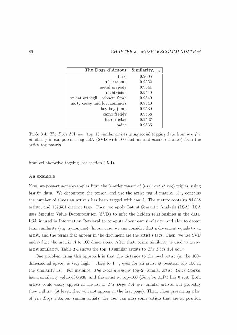
86 CHAPTER 3. MUSIC RECOMMENDATION
The Dogs d’Amour SimilarityLSA
d-a-d 0.9605mike tramp 0.9552
metal majesty 0.9541nightvision 0.9540
bulent ortacgil - sebnem ferah 0.9540marty casey and lovehammers 0.9540
hey hey jump 0.9539camp freddy 0.9538hard rocket 0.9537
paine 0.9536
Table 3.4: The Dogs d’Amour top–10 similar artists using social tagging data from last.fm.Similarity is computed using LSA (SVD with 100 factors, and cosine distance) from theartist–tag matrix.
from collaborative tagging (see section 2.5.4).
An example
Now, we present some examples from the 3–order tensor of 〈user, artist, tag〉 triples, using
last.fm data. We decompose the tensor, and use the artist–tag A matrix. Ai,j contains
the number of times an artist i has been tagged with tag j. The matrix contains 84,838
artists, and 187,551 distinct tags. Then, we apply Latent Semantic Analysis (LSA). LSA
uses Singular Value Decomposition (SVD) to infer the hidden relationships in the data.
LSA is used in Information Retrieval to compute document similarity, and also to detect
term similarity (e.g. synonyms). In our case, we can consider that a document equals to an
artist, and the terms that appear in the document are the artist’s tags. Then, we use SVD
and reduce the matrix A to 100 dimensions. After that, cosine similarity is used to derive
artist similarity. Table 3.4 shows the top–10 similar artists to The Dogs d’Amour.
One problem using this approach is that the distance to the seed artist (in the 100–
dimensional space) is very high —close to 1—, even for an artist at position top–100 in
the similarity list. For instance, The Dogs d’Amour top–20 similar artist, Gilby Clarke,
has a similarity value of 0.936, and the artist at top–100 (Babylon A.D.) has 0.868. Both
artists could easily appear in the list of The Dogs d’Amour similar artists, but probably
they will not (at least, they will not appear in the first page). Then, when presenting a list
of The Dogs d’Amour similar artists, the user can miss some artists that are at position
3.4. RECOMMENDATION METHODS 87
top–80, and that are still relevant. This happens because the semantic distance based on
tags (using the 100 factors after applying SVD) is very coarse. To overcome this problem,
in the following section we present a hybrid approach that combines collaborative filtering
and social tagging, producing more reliable results.
3.4.4 Hybrid methods
The combination of different approaches allows a system to minimise the issues that a solely
method can have. One way to combine different recommendation methods is the cascade
approach (see section 2.5.5). Cascade is a step by step process. One technique is applied
first, obtaining a ranked list of items. Then, a second technique refines or re–rank the
results obtained in the first step.
To compute artist similarity a system can first apply CF, and then reorder and combine
the results according to the semantic distance from social tagging (LSA).
An example
Table 3.5 shows The Dogs d’Amour similar artists using a cascade hybrid method. First,
The Dogs d’Amour top–100 similar artists are computed using CF, with Pearson correlation
distance. In a second step, for each artist in this top–100 list we compute LSA —using SVD
with 100 factors— and cosine similarity from the social tagging data, between the actual
artist and the seed artist (The Dogs d’Amour). After that, we combine the results from
Pearson CF with the results obtained in this second step. We use a linear combination
function setting α = 0.5:
sim(ai, aj)Hybrid = (1 − α) · sim(ai, aj)CF,Pearson + α · sim(ai, aj)Context,LSA (3.3)
This way we can improve the original CF results, and also the results obtained solely from
social tagging. Indeed, the Pearson CF approach returned some strange and non–relevant
results, such as Michael Jackson or Zero 7 (see Table 3.5, left). After reordering the results,
both artists disappear. Also, some artists that were not in the CF top–10 appear in the final
set of similar artists (Table 3.5, right), due to the linear combination of the two approaches
(Pearson CF and LSA from tags).
In this case, the cascade chain method makes sense. The first results are obtained taking
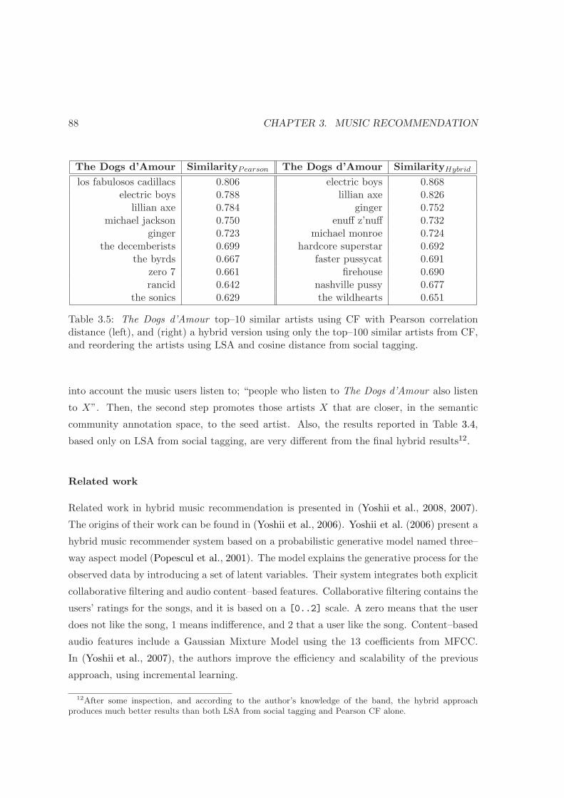
88 CHAPTER 3. MUSIC RECOMMENDATION
The Dogs d’Amour SimilarityPearson The Dogs d’Amour SimilarityHybrid
los fabulosos cadillacs 0.806 electric boys 0.868electric boys 0.788 lillian axe 0.826
lillian axe 0.784 ginger 0.752michael jackson 0.750 enuff z’nuff 0.732
ginger 0.723 michael monroe 0.724the decemberists 0.699 hardcore superstar 0.692
the byrds 0.667 faster pussycat 0.691zero 7 0.661 firehouse 0.690rancid 0.642 nashville pussy 0.677
the sonics 0.629 the wildhearts 0.651
Table 3.5: The Dogs d’Amour top–10 similar artists using CF with Pearson correlationdistance (left), and (right) a hybrid version using only the top–100 similar artists from CF,and reordering the artists using LSA and cosine distance from social tagging.
into account the music users listen to; “people who listen to The Dogs d’Amour also listen
to X”. Then, the second step promotes those artists X that are closer, in the semantic
community annotation space, to the seed artist. Also, the results reported in Table 3.4,
based only on LSA from social tagging, are very different from the final hybrid results12.
Related work
Related work in hybrid music recommendation is presented in (Yoshii et al., 2008, 2007).
The origins of their work can be found in (Yoshii et al., 2006). Yoshii et al. (2006) present a
hybrid music recommender system based on a probabilistic generative model named three–
way aspect model (Popescul et al., 2001). The model explains the generative process for the
observed data by introducing a set of latent variables. Their system integrates both explicit
collaborative filtering and audio content–based features. Collaborative filtering contains the
users’ ratings for the songs, and it is based on a [0..2] scale. A zero means that the user
does not like the song, 1 means indifference, and 2 that a user like the song. Content–based
audio features include a Gaussian Mixture Model using the 13 coefficients from MFCC.
In (Yoshii et al., 2007), the authors improve the efficiency and scalability of the previous
approach, using incremental learning.
12After some inspection, and according to the author’s knowledge of the band, the hybrid approachproduces much better results than both LSA from social tagging and Pearson CF alone.
3.5. SUMMARY 89
Tiemann and Pauws (2007) investigate ensemble learning methods for hybrid music
recommender algorithms. It combines social and content–based recommender algorithms.
Each method produce a weak learner. Then, using a combination rule, it unifies the out-
put of the weak learners. The results suggests that the hybrid approach reduces the mean
absolute prediction error, compared to the weak learners used solely.
3.5 Summary
This chapter has presented all the elements of music recommendation; user profile and item
representation, and the existing recommendation methods.
User preferences depends on the type of listener, and her level of engagement with
the music. Furthermore, music perception is very subjective, and it is influenced by the
context. In this sense, user profile representation is an important aspect. We have presented
three different notations: UMIRL, MPEG-7 based, and FOAF. The former is one of the
first attempts in this field. The UMIRL language is not formal enough, but a proposal
that contains some interesting ideas. User preferences in MPEG-7 is the first big and
serious attempt to formalise user modelling, related with the multimedia content. The
main problem of this approach is that the MPEG-7 standard is too complex and verbose.
It is not straight forward to generate user profiles following the notation proposed by the
standard. The last proposal, FOAF profiles, is based on the Semantic Web initiative. It is
the most flexible approach. As it is based on the Semantic Web premises, FOAF profiles
can embed different ontologies, so it is extensible, and has richer semantics than the other
two approaches.
In music recommedation, item–based similarity is the most common way to predict the
recommendations. Item profile representation is the first step to compute item similarity,
and to provide recommendations to the users. Some recommendations for a rock band, The
Dogs d’Amour, are also provided for most of the recommendation methods presented. An
informal evaluation shows that a hybrid approach, using a mix of CF and context–based
filtering from social tagging, produces the most interesting results.
Links with the following chapters
An important remaining task is the formal evaluation of item (and user) similarity, as it
is the basis to provide music recommendations. This evaluation is presented in chapters

90 CHAPTER 3. MUSIC RECOMMENDATION
5, that presents the metrics, and 6, that contains the actual evaluation of real, and big
datasets. Also, the user’s perceived quality of the recommendations is very important. We
present, in chapter 7, an experiment done with 288 subjects, that analyses the effects of
providing novel and relevant recommendations to users.
Chapter 4
The Long Tail in recommender
systems
4.1 Introduction
The Long Tail is composed of a small number of popular items, the well–known hits, and
the rest are located in the heavy tail, those not sell that well. The Long Tail offers the
possibility to explore and discover —using automatic tools; such as recommenders or per-
sonalised filters— vast amounts of data. Until now, the world was ruled by the Hit or Miss
categorisation, due in part to the shelf space limitation of the brick–and–mortar stores.
A world where a music band could only succeed selling millions of albums, and touring
worldwide.
Nowadays, we are moving towards the Hit vs. Niche paradigm, where there is a large
enough availability of choice to satisfy even the most “Progressive–obscure–Spanish–metal”
fan. The problem, though, is to filter and present the right artists to the user, according to
her musical taste.
Chris Anderson introduces in his book, “The Long Tail”, a couple of important con-
ditions to exploit the content available in niche markets. These are: (i) make everything
available, and (ii) help me find it (Anderson, 2006). It seems that the former condition is
already fulfilled; the distribution and inventory costs are nearly negligible. Yet, to satisfy
the latter we need recommender systems that exploit the “from hits to niches” paradigm.
The main question, though, is whether current recommendation techniques are ready to as-
sist us in this discovery task, providing recommendations of the hidden jewels in the Long
91
92 CHAPTER 4. THE LONG TAIL IN RECOMMENDER SYSTEMS
Tail.
In fact, recommenders that appropriately discount popularity may increase total sales,
as well as potentially increase the margins by suggesting more novel, or less known, products
(Fleder and Hosanagar, 2007). Tucker and Zhang (2008) develop a theoretical model which
shows how the existence of popular items can, in fact, benefit the perceived quality of niche
products. As these niche items are less likely to attract customers, the ones they attract
perceive the products as higher quality than the mainstream ones. The authors’ findings
contribute to the understanding that popularity affects the long tail of e-Commerce. Even
though web 2.0 tools based on the user’s history of purchases promote the popular goods,
their results suggest that mainstreamness benefits the perceived quality of niche products.
Again, the big problem is to develop filters and tools that allow users to find and discover
these niche products.
Pre– and post–filters
In the brick–and–mortar era, the market pre–filtered those products with lower probability
of being bought by people. The main problem was the limited physical space to store the
goods. Nowadays, with the unlimited shelf space, there is no need to pre–filter any product
(Anderson, 2006). Instead, what users need are post–filters to make the products available
and visible, and get personalised recommendations, according to their interests. Still, when
publishers or producers pre–filter the content they also contribute to cultural production.
E.g. many books or albums would be a lot worse without their editors and producers.
One should assume that there are some extremely poor quality products along the Long
Tail. These products do not need to be removed by the gatekeepers anymore, but can
remain in the Long Tail forever. The advisors are the ones in charge of not recommending
low quality goods. In this sense, Salganik et al. (2006) proved that increasing the strength of
social influence increased both inequality and unpredictability of success. As a consequence,
popularity was only partly determined by quality. In fact, the quality of a work cannot be
assessed in isolation, because our experience is so tied up with other people’s experience of
that work. Therefore, one can find items to match anyone’s taste along the Long Tail. It is
the job of the post–filters to ease the task of finding them.
4.2. THE MUSIC LONG TAIL 93
4.2 The Music Long Tail
As already mentioned in Chapter 1, the “State of the Industry” report (Soundscan, 2007)
presents some insights about the long tail in music consumption. For instance, 844 mil-
lion digital tracks were sold in 2007, but only 1% of all digital tracks—the head part of
the curve—accounted for 80% of all track sales. Also, 1,000 albums accounted for 50%
of all album sales, and 450,344 of the 570,000 albums sold were purchased less than 100
times. Music consumption is biased towards a few mainstream artists. Ideally, by provid-
ing personalised filters and discovery tools to the listeners, music consumption would be
diversified.
The Long Tail of sales versus the Long Tail of plays
When computing a Long Tail distribution, one should define how to measure the popularity
of the items. In the music domain, this can be achieved using the total number of sales or
the total number of plays. On the one hand, the total number of sales denote the current
trends in music consumption. On the other hand, the total number of playcounts tell us
what people listen to, independently of the release year of the album (or song).
In terms of coverage, total playcounts is more useful, as it can represent a larger number
of artists. An artist does not need to have an album released, but a Myspace–like page,
which includes the playcounts for each song. Gathering information about the number of
plays is easier than collecting the albums an artist has sold. Usually, the number of sales are
shown in absolute values, aggregating all the information, and these numbers are used to
compare the evolution of music consumption over the years. The total number of plays give
us more accurate information, as it describes what people listen to. Thus, we will define
the Long Tail in music using the total playcounts per artist.
As an example, Table 4.1 shows the overall most played artists at last.fm in July, 2007.
These results come from more than 20 million registered users. Although the list of top–10
artists are biased towards this set of users, it still represents the listening habits of a large
amount of people. In contrast, Table 4.2 shows the top–10 artists in 2006 based on total
digital track sales (last column) according to Soundscan (2006) report. The second column
(values in parenthesis) shows the corresponding last.fm artist rank. There is not a clear
correlation between the two lists, and only one artist (Red Hot Chili Peppers) appears in
both top–10 lists.
94 CHAPTER 4. THE LONG TAIL IN RECOMMENDER SYSTEMS
1. The Beatles (50,422,827)
2. Radiohead (40,762,895)
3. System of a Down (37,688,012)
4. Red Hot Chili Peppers (37,564,100)
5. Muse (30,548,064)
6. Death Cab for Cutie (29,335,085)
7. Pink Floyd (28,081,366)
8. Coldplay (27,120,352)
9. Nine Inch Nails (24,095,408)
10. Blink 182 (23,330,402)
Table 4.1: Top–10 popular artists in last.fm according to the total number of plays (lastcolumn). Data gathered during July, 2007.
1. (912) Rascal Flatts (3,792,277)
2. (175) Nickelback (3,715,579)
3. (205) Fray (3,625,140)
4. (154) All-American Rejects (3,362,528)
5. (119) Justin Timberlake (3,290,523)
6. (742) Pussycat Dolls (3,277,709)
7. (4) Red Hot Chili Peppers (3,254,306)
8. (92) Nelly Furtado (3,052,457)
9. (69) Eminem (2,950,113)
10. (681) Sean Paul (2,764,505)
Table 4.2: Top–10 artists in 2006 based on total digital track sales (last column) accordingto Nielsen report (Soundscan, 2006). The second column (values in parenthesis) shows thecorresponding last.fm artist rank.
4.2. THE MUSIC LONG TAIL 95
1. (912) Rascal Flatts (4,970,640)
2. (70) Johnny Cash (4,826,320)
3. (175) Nickelback (3,160,025)
4. (1514) Carrie Underwood (3,016,123)
5. (1) The Beatles (2,812,720)
6. (1568) Tim McGraw (2,657,675)
7. (2390) Andrea Bocelli (2,524,681)
8. (1575) Mary J. Blige (2,485,897)
9. (1606) Keith Urban (2,442,577)
10. (119) Justin Timberlake (2,437,763)
Table 4.3: Top–10 selling artists in 2006 (based on total album sales, last column) accordingto Nielsen report (Soundscan, 2006). The second column (values in parenthesis) shows thecorresponding last.fm artist rank.
Furthermore, Table 4.3 shows the top–10 selling artists in 2006 based on total album
sales (last column), again according to the Nielsen report (Soundscan, 2006). In this case,
classic artists such as Johnny Cash (top–2) or The Beatles (top–5) appear. This reflects the
type of users that still buy CDs. Regarding Carrie Underwood, she is an American country
pop music singer who became famous after winning the fourth season of American Idol
(2005). Carrie Underwood album, released in late 2005, became the fastest selling debut
Country album. Keith Urban, Tim McGraw and Rascal Flatts are American country/pop
songwriters with a leading male singer. In all these cases, they are not so popular in the
last.fm community.
All in all, only The Beatles (in Table 4.3), and Red Hot Chili Peppers (in Table 4.2)
appear in the top-10 last.fm chart (see Table 4.1). It is worth noting that in 2006 The Beatles
music collection was not (legally) available for purchase in digital form. On the other hand,
last.fm listening habits denote what people listen to, and that does not necessarily correlate
with the best sellers. For instance, classic bands such as Pink Floyd, Led Zeppelin (at top–
15), Tool (top–16) or Nirvana (top–18) did not release any new album during 2006, but
still they are in the top–20 (at mid–2007). From this informal analysis we conclude that
popularity is a nebulous concept that can be viewed in different ways.
From now on, we characterise music popularity using the total playcounts of an artist,
keeping in mind that the data is not correlated with the actual number of sales, and also
that the data will be biased towards the subset of users that are taken into account (in our
case, the entire last.fm community).
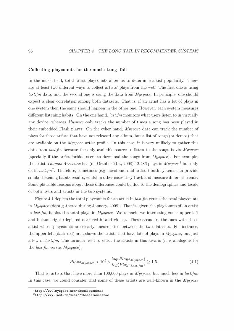
96 CHAPTER 4. THE LONG TAIL IN RECOMMENDER SYSTEMS
Collecting playcounts for the music Long Tail
In the music field, total artist playcounts allow us to determine artist popularity. There
are at least two different ways to collect artists’ plays from the web. The first one is using
last.fm data, and the second one is using the data from Myspace. In principle, one should
expect a clear correlation among both datasets. That is, if an artist has a lot of plays in
one system then the same should happen in the other one. However, each system measures
different listening habits. On the one hand, last.fm monitors what users listen to in virtually
any device, whereas Myspace only tracks the number of times a song has been played in
their embedded Flash player. On the other hand, Myspace data can track the number of
plays for those artists that have not released any album, but a list of songs (or demos) that
are available on the Myspace artist profile. In this case, it is very unlikely to gather this
data from last.fm because the only available source to listen to the songs is via Myspace
(specially if the artist forbids users to download the songs from Myspace). For example,
the artist Thomas Aussenac has (on October 21st, 2008) 12,486 plays in Myspace1 but only
63 in last.fm2. Therefore, sometimes (e.g. head and mid artists) both systems can provide
similar listening habits results, whilst in other cases they track and measure different trends.
Some plausible reasons about these differences could be due to the demographics and locale
of both users and artists in the two systems.
Figure 4.1 depicts the total playcounts for an artist in last.fm versus the total playcounts
in Myspace (data gathered during January, 2008). That is, given the playcounts of an artist
in last.fm, it plots its total plays in Myspace. We remark two interesting zones upper left
and bottom right (depicted dark red in and violet). These areas are the ones with those
artist whose playcounts are clearly uncorrelated between the two datasets. For instance,
the upper left (dark red) area shows the artists that have lots of plays in Myspace, but just
a few in last.fm. The formula used to select the artists in this area is (it is analogous for
the last.fm versus Myspace):
PlaysMyspace > 105 ∧ log(PlaysMyspace)
log(PlaysLast.fm)≥ 1.5 (4.1)
That is, artists that have more than 100,000 plays in Myspace, but much less in last.fm.
In this case, we could consider that some of these artists are well–known in the Myspace
1http://www.myspace.com/thomasaussenac2http://www.last.fm/music/thomas+aussenac
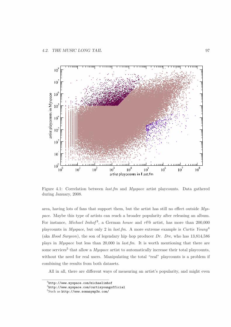
4.2. THE MUSIC LONG TAIL 97
Figure 4.1: Correlation between last.fm and Myspace artist playcounts. Data gatheredduring January, 2008.
area, having lots of fans that support them, but the artist has still no effect outside Mys-
pace. Maybe this type of artists can reach a broader popularity after releasing an album.
For instance, Michael Imhof 3, a German house and r&b artist, has more than 200,000
playcounts in Myspace, but only 2 in last.fm. A more extreme example is Curtis Young4
(aka Hood Surgeon), the son of legendary hip–hop producer Dr. Dre, who has 13,814,586
plays in Myspace but less than 20,000 in last.fm. It is worth mentioning that there are
some services5 that allow a Myspace artist to automatically increase their total playcounts,
without the need for real users. Manipulating the total “real” playcounts is a problem if
combining the results from both datasets.
All in all, there are different ways of measuring an artist’s popularity, and might even
3http://www.myspace.com/michaelimhof4http://www.myspace.com/curtisyoungofficial5Such as http://www.somanymp3s.com/
98 CHAPTER 4. THE LONG TAIL IN RECOMMENDER SYSTEMS
Figure 4.2: The Long Tail for artist popularity. A log–linear plot depicting the total numberof plays. Data gathered during July, 2007, for a list of 260,525 artists.
exist different domains of popularity; what is popular in one domain can be unknown in
another. As previously stated, popularity is a nebulous concept that can be viewed in
different ways.
An example
Figure 4.2 depicts the Long Tail popularity, using total playcounts, for 260,525 music artists.
The horizontal axis contains the list of artists ranked by its total playcounts. E.g. The
Beatles, at position 1, has more than 50 million playcounts.
This data was gathered from last.fm during July, 2007. Last.fm provides plugins for
almost any desktop music player (as well as iPhones and other mobile devices) to track users’
listening behaviour. It also provides a Flash player embedded in their website, and a client
for PC, Mac and Linux that can create personalised audio streams. Figure 4.2 corroborates
the music consumption reports by Nielsen (Soundscan, 2007); a few artists concentrate most

4.3. DEFINITIONS 99
Figure 4.3: The Long Tail for artist popularity. Same plot as Figure 4.2 in log–log scale.The best fit is a log–normal distribution, with a mean of log µ = 6.8, and standard deviationof log, σ = 2.18. The fast drop in the tail is in part due to misspelled artists (e.g. incorrectmetadata in the ID3 tags).
of the total plays, whilst many musicians hold the rest. Figure 4.3 presents the same data
as Figure 4.2, in log–log scale. The best fit for the curve is a log–normal distribution, with
parameters mean of log µ = 6.8, and standard deviation of log σ = 2.18 (more information
about fitting a curve with a distribution model is presented in section 4.3.2). It is worth
noting that the fast drop in the tail is in part due to misspelled artists (e.g. incorrect
metadata in the ID3 tags).
4.3 Definitions
The Long Tail of a catalog is measured using the frequency distribution (e.g. purchases,
downloads, etc.), ranked by item popularity. We present now two definitions for the Long
Tail. The first one is an informal, intuitive one. The second one is a quantitative definition
100 CHAPTER 4. THE LONG TAIL IN RECOMMENDER SYSTEMS
that uses a formal model to characterise the shape of the curve, and a method to fit the
data to some well–known distributions (e.g. power–law, power–law with exponential decay,
log–normal, etc.)
4.3.1 Qualitative, informal definition
According to Anderson (2006), the Long Tail is divided in two separate parts: the head
and the tail. The head part contains the items one can find in the old brick–and–mortar
markets. The tail of the curve is characterised by the remainder of the existing products.
This includes the items that are available in on–line markets. Chris Anderson’s definition,
based on the economics of the markets, is:
“The Long Tail is about the economics of abundance; what happens when
the bottlenecks that stand between supply and demand in our culture start to
disappear and everything becomes available to everyone”.
The definition emphasises the existence of two distinguished markets; the familiar one
(the Head), and the long ignored but emerging since the explosion of the web (the Tail),
consisting of small niche markets.
Another definition is the one by Jason Foster:
“The Long Tail is the realization that the sum of many small markets is
worth as much, if not more, than a few large markets”.6
Both definitions are based on markets and economics, and do not propose any compu-
tational model to compute and characterise any tail curve, nor fit the data to any existing
distribution. Indeed, Anderson (2006) does not define how to split the head and the tail
parts, that are the two key elements in both definitions.
Physical apples versus online oranges
Since The Long Tail book became a top–seller, there is a lot of criticism against Ander-
son’s theory. The most common criticism is the lack of scientific backup when comparing
different data sources. That is, when comparing the online world to the physical world,
Anderson simplifies too much. For instance, he considers only one brick–and–mortar store
6From http://www.thelongtail.com/the_long_tail/2005/01/definitions_fin.html

4.3. DEFINITIONS 101
(e.g. Walmart), and compares their music catalog with the one found in the Rhapsody
online store. However, in the real world there are much more music stores than Walmart.
Indeed, there are specialised music stores that carry out ten times the volume of Walmart ’s
music catalog. Sadly enough, these ones are completely ignored in Anderson’s studies (Slee,
2006).
In addition, there is no clear evidence that online stores can monetise the Long Tail.
According to Elberse (2008), there is no evidence of a shift in online markets towards
promoting the tail. The tail is long, but extremely flat. In their results, hit–driven
economies are found in both physical and online markets. Furthermore, in an older study,
Elberse and Oberholzer-Gee (2006) found that the long tail of movies, those that sell only
a few copies every week nearly doubled during their study period. However, the number of
non–selling titles rose four times, thus increasing the size of the tail. Regarding the head of
the curve; a few mainstream movies still accounted for most of the sales.
Another drawback of the theory is the creation of online oligarchies. “Make every-
thing available” is commonly achieved by One–Big–Virtual–Tent rather than Many–Small–
Tents7. That is to say, there is only one Amazon that provides most of the content.
Last but not least, Anderson’s theory states that the Long Tail follows a power–law
distribution. That is a straight line in a log–log plot. However, only plotting a curve in a
log–log scale is not enough to verify that the curve follows a power–law. It can better fit
to other distributions, such as log–normal or a power–law with an exponential decay of the
tail. We need, then, a model that allows us to quantitative define the shape of the Long
Tail curve, without the need of linking it with niche markets, economics, or profitable (or
not) e–Commerce websites.
4.3.2 Quantitative, formal definition
The Long Tail model, F (x), simulates any heavy–tailed distribution (Kilkki, 2007). It
models the cumulative distribution of the Long Tail data. F (x) represents the share (%) of
total volume covered by objects up to rank x:
F (x) =β
(N50x )α + 1
(4.2)
7See Tom Slee critical reader’s companion to “The Long Tail” book athttp://whimsley.typepad.com/whimsley/2007/03/the_long_tail_l.html
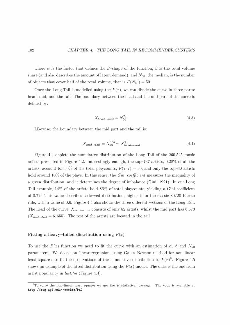
102 CHAPTER 4. THE LONG TAIL IN RECOMMENDER SYSTEMS
where α is the factor that defines the S–shape of the function, β is the total volume
share (and also describes the amount of latent demand), and N50, the median, is the number
of objects that cover half of the total volume, that is F (N50) = 50.
Once the Long Tail is modelled using the F (x), we can divide the curve in three parts:
head, mid, and the tail. The boundary between the head and the mid part of the curve is
defined by:
Xhead→mid = N2/350 (4.3)
Likewise, the boundary between the mid part and the tail is:
Xmid→tail = N4/350 ≃ X2
head→mid (4.4)
Figure 4.4 depicts the cumulative distribution of the Long Tail of the 260,525 music
artists presented in Figure 4.2. Interestingly enough, the top–737 artists, 0.28% of all the
artists, account for 50% of the total playcounts, F (737) = 50, and only the top–30 artists
hold around 10% of the plays. In this sense, the Gini coefficient measures the inequality of
a given distribution, and it determines the degree of imbalance (Gini, 1921). In our Long
Tail example, 14% of the artists hold 86% of total playcounts, yielding a Gini coefficient
of 0.72. This value describes a skewed distribution, higher than the classic 80/20 Pareto
rule, with a value of 0.6. Figure 4.4 also shows the three different sections of the Long Tail.
The head of the curve, Xhead→mid consists of only 82 artists, whilst the mid part has 6,573
(Xmid→tail = 6, 655). The rest of the artists are located in the tail.
Fitting a heavy–tailed distribution using F (x)
To use the F (x) function we need to fit the curve with an estimation of α, β and N50
parameters. We do a non–linear regression, using Gauss–Newton method for non–linear
least squares, to fit the observations of the cumulative distribution to F (x)8. Figure 4.5
shows an example of the fitted distribution using the F (x) model. The data is the one from
artist popularity in last.fm (Figure 4.4).
8To solve the non–linear least squares we use the R statistical package. The code is available athttp://mtg.upf.edu/~ocelma/PhD

4.3. DEFINITIONS 103
Figure 4.4: Example of the Long Tail model. It shows the cumulative percentage of play-counts of the 260,525 music artists from Figure 4.2. Only top–737 artists, 0.28% of allthe artists, accumulates the 50% of total playcounts (N50). Also, the curve is divided inthree parts: head, mid and tail (Xhead→mid = 82, and Xmid→tail = 6, 655), so each artist islocated in one section of the curve.
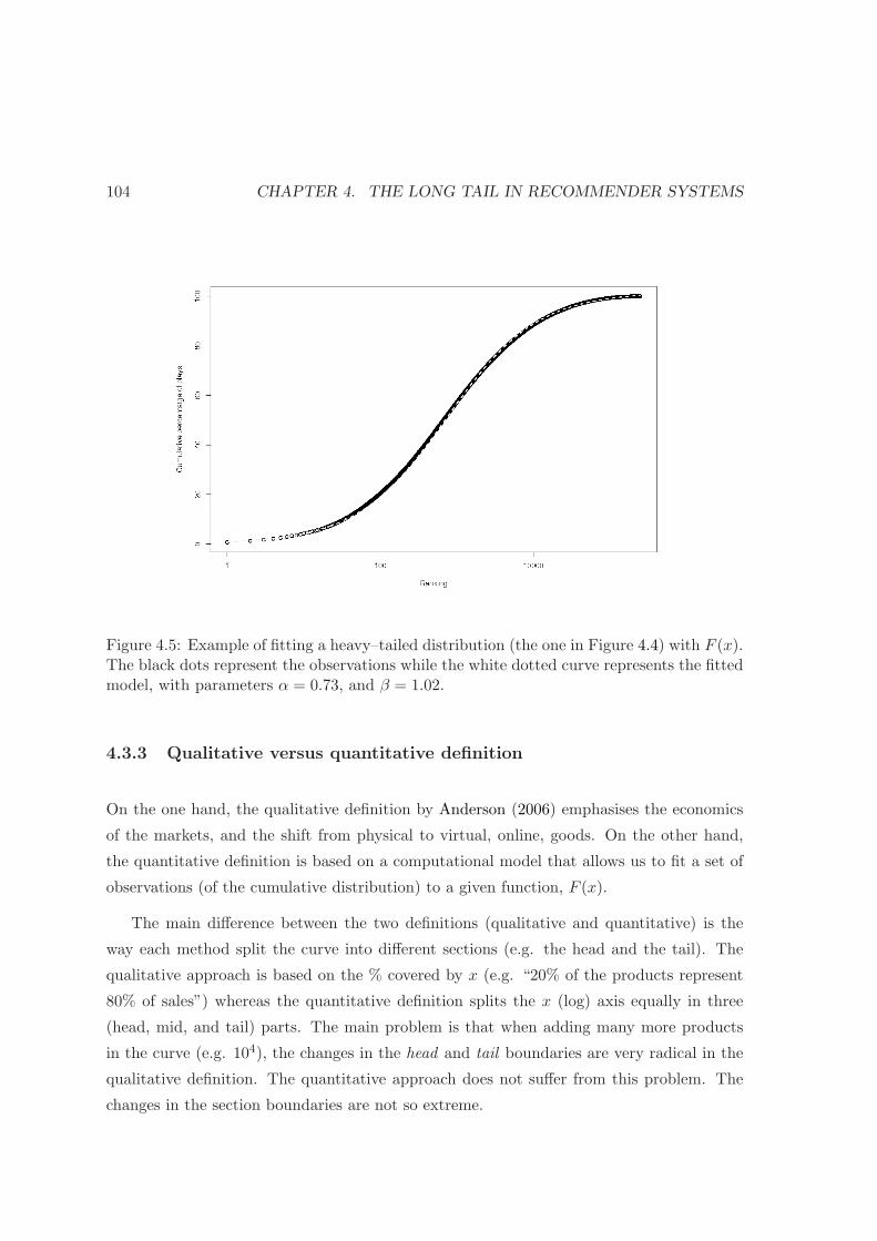
104 CHAPTER 4. THE LONG TAIL IN RECOMMENDER SYSTEMS
Figure 4.5: Example of fitting a heavy–tailed distribution (the one in Figure 4.4) with F (x).The black dots represent the observations while the white dotted curve represents the fittedmodel, with parameters α = 0.73, and β = 1.02.
4.3.3 Qualitative versus quantitative definition
On the one hand, the qualitative definition by Anderson (2006) emphasises the economics
of the markets, and the shift from physical to virtual, online, goods. On the other hand,
the quantitative definition is based on a computational model that allows us to fit a set of
observations (of the cumulative distribution) to a given function, F (x).
The main difference between the two definitions (qualitative and quantitative) is the
way each method split the curve into different sections (e.g. the head and the tail). The
qualitative approach is based on the % covered by x (e.g. “20% of the products represent
80% of sales”) whereas the quantitative definition splits the x (log) axis equally in three
(head, mid, and tail) parts. The main problem is that when adding many more products
in the curve (e.g. 104), the changes in the head and tail boundaries are very radical in the
qualitative definition. The quantitative approach does not suffer from this problem. The
changes in the section boundaries are not so extreme.
4.4. CHARACTERISING A LONG TAIL DISTRIBUTION 105
4.4 Characterising a Long Tail distribution
An early mention of the “long tail”, in the context of the Internet, was Clay Shirky’s essay
in February, 20039. After that, Anderson (2006) converted the term to a proper noun, and
defined a new trend in economics. Since then, the spotlight on the “Long Tail” noun has
created many different opinions about it.
In our context, we use a “Long Tail” curve to describe the popularity phenomenon in
any recommender system, to show how popularity can affect the recommendations. So,
given a long tail distribution of the items’ popularity, an important step is to characterise
the shape of the curve to understand the amount of skewness. We characterise a Long Tail
distribution using Kilkki’s function F (x). Its parameters α, β, and N50 defines the shape
of the curve. Yet, it is also important to determine the shape of the curve according to
well–known probability density distributions.
Not all Long Tails are power–law
There are different probability density distribution functions that can fit a heavy–tailed
curve. We present some of them here: power–law, power–law with exponential decay, and
log–normal distribution.
A power–law distribution is described using the probability density distribution
(pdf ), f(x):
f(x) = ax−γ (4.5)
Power–law distribution has the property of (asymptotic) scale invariance. This type
of distribution cannot be entirely characterised by its mean and variance. Also, if the γ
power–law exponent has a value close to 1, γ ≃ 1, then this means that the long tail is
fat10. In other words, a power–law with γ ≫ 1 consists of a thin tail (with values close to
0), and a short head with a high probability value.
Power–law with an exponential decay distribution differs from a power–law by the
shape of the tail. Its pdf is defined by:
f(x) = x−γe−λx, (4.6)
9See http://shirky.com/writings/powerlaw_weblog.html10This is the only case where Anderson’s Long Tail theory can be applied.
106 CHAPTER 4. THE LONG TAIL IN RECOMMENDER SYSTEMS
There exists an N that denotes the threshold between the power–law distribution
(x ≤ N), and the exponential decay (x > N). This means that, sometimes, there is a
characteristic scale in the power–law that is better represented with an exponential cut–off.
In a log–normal distribution the logarithm of the variable is normally distributed.
That is to say, if a variable X is normally distributed, then Y = eX has a log–normal
distribution. Log–normal distribution promotes the head of the curve. It is a distribution
skewed to the right, where the popular items have a strong effect, whilst the tail has a very
small contribution in the pdf :
f(x) =1
xe−
(ln(x)−µ)2
2σ2 (4.7)
Thus, the main problem is, given a curve —in a log–log scale representation—, to
decide which is the best model that explains the curve. It is worth noting that, according
to Anderson’s theory (i.e. the Long Tail is profitable), the curve should be modelled as
a power–law, with γ ≃ 1, meaning that the tail is fat. However, if the best fit is using
another distribution, such as a log–normal —which is very common—, then Anderson’s
theory cannot be strictly applied in that particular domain and context.
A model selection: power–law or not power–law?
To characterise a heavy–tailed distribution, we follow the steps described in (Clauset et al.,
2007). As previously mentioned, the main drawbacks when fitting a Long Tail distribution
are: (i) to plot the distribution on a log–log plot, and see whether it follows a straight line or
not, and (ii) use linear regression by least squares to fit a line in the log–log plot, and then
use R2 to measure the fraction of variance accounted for the curve. This approach gives a
poor estimate of the model parameters, as it is meant to be applied to regression curves,
not to compare distributions. Instead, to decide whether a heavy–tailed curve follows a
power–law distribution, Clauset et al. (2007) propose the following steps:
1. Estimate γ. Use the maximum likelihood estimator (MLE) for the γ scaling expo-
nent. MLE always converge to the correct value of the scaling exponent.
2. Detect xmin. Use the goodness of fit value to estimate where the scaling region
begins (xmin). The curve can follow a power–law on the right or upper tail, so above
a given threshold xmin. The authors propose a method that can empirically find the
best scaling region, based on the Kolmogorov–Smirnov D statistic.

4.5. THE DYNAMICS OF THE LONG TAIL 107
3. Goodness of the model. Use, again, the Kolmogorov–Smirnov D statistic to com-
pute the discrepancy between the empirical distribution and the theoretical one. The
Kolmogorov–Smirnov (K–S) D statistic will converge to zero, if the empirical distri-
bution follows the theoretical one (e.g. power–law). The K–S D statistic for a given
cumulative distribution function F (x), and its empirical distribution function Fn(x)
is:
Dn = supx
|Fn(x) − F (x)|, (4.8)
where sup S is the supremum of set S. The supremum of S is the lowest element
of F (x) that is greater than or equal to each element of S. The supremum is also
referred to as the least upper bound.
4. Model selection. Once the data is fitted to a power–law distribution, the only re-
maining task is to check among the different alternatives. That is, to detect whether
other non power–law distributions could have produced the data. This is done us-
ing pairwise comparison (e.g. power–law versus power–law with exponential decay,
power–law versus a log–normal, etc.), and Clauset et al. (2007) use the Vuong’s test
(Vuong, 1989). Vuong’s test uses the log–likelihood ratio, and the Kullback–Leibler
information criterion to make probabilistic statements about the two models. Vuong’s
statistical test is used for the model selection problem, where one can determine which
distribution is closer to the real data. A large, positive Vuong’s test statistic provides
evidence of the best fitting using a power–law distribution over the other distribution,
while a large, negative test statistic is an evidence of the contrary.
4.5 The dynamics of the Long Tail
An important aspect of any Long Tail is its dynamics. E.g., does an artist stay in the head
region forever? Or the other way around; will niche artists always remain in the long tail?
Figure 4.6 depicts the increase of the Long Tail popularity after 6 months, using 50,000 out
of the 260,525 last.fm artists (see Figure 4.2). Figure 4.6 shows the dynamics of the curve
comparing two snapshots; one from July 2007, and the other from January 2008. The most
important aspect is the increase of total playcounts in each area of the curve.
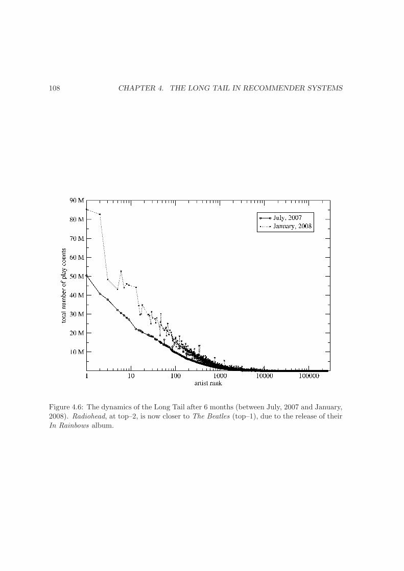
108 CHAPTER 4. THE LONG TAIL IN RECOMMENDER SYSTEMS
Figure 4.6: The dynamics of the Long Tail after 6 months (between July, 2007 and January,2008). Radiohead, at top–2, is now closer to The Beatles (top–1), due to the release of theirIn Rainbows album.
4.6. NOVELTY, FAMILIARITY AND RELEVANCE 109
Long Tail region Increase (%)
Head 61.20
Mid 62.29
Tail 62.32
Table 4.4: Increase of the Long Tail regions (in %) after 6 months (comparing two snapshotsin July, 2007 and January, 2008).
Strike a chord?
Table 4.4 shows the playcount increment, in %. In all the three regions —head, mid, and
tail— the percentage increment of plays is almost the same (around 62%), meaning that
not many artists move between the regions. For instance, in the head area, Radiohead at
top–2 is much closer to top–1, The Beatles, due to the release of the In Rainbows album.
Still, the band remains at top–2. An interesting example in the tail area is the Nulla Costa
band. This band was at rank 259,962 in July, 2007. After six months they increase from
3 last.fm playcounts to 4,834, positioning at rank 55,000. Yet, the band is still in the tail
region. We could not detect any single artist that clearly moved from the tail to the mid
region11. There exist niche artists, and the main problem is to find them. The only way to
leverage the long tail is by providing recommendations that promote unknown artists.
Once the Long Tail is formally described, the next step is to use this knowledge when
providing recommendations. The following section presents how one can exploit the Long
Tail to provide novel or familiar recommendations, taking into account the user profile.
4.6 Novelty, familiarity and relevance
“If you like The Beatles you might like...X”. Now, ask several different people and you will
get lots of different X ′s. Each person, according to her ties with the band’s music, would
be able to propose interesting, surprising or expected X ′s. Nonetheless, asking the same
question to different recommender systems we are likely to get similar results. Indeed, two
out of five tested music recommenders contain John Lennon, Paul McCartney and George
Harrison in their top–10 (last.fm and the.echotron.com). Yahoo! Music recommends John
Lennon and Paul McCartney (1st and 4th position), whereas Mystrands.com only contains
11Last.fm has the “hype artist” weekly chart, http://www.last.fm/charts/hypeartist, a good sourceto track the movements in the Long Tail curve.

110 CHAPTER 4. THE LONG TAIL IN RECOMMENDER SYSTEMS
John Lennon (at top–10). Neither ilike nor Allmusic.com contain any of these musicians
in their list of Beatles’ similar artists. Furthermore, Amazon’s top–30 recommendations
for the Beatles’ White Album is strictly made of other Beatles’ albums (all of a sudden, at
the fourth page of the navigation there is the first non–Beatles album; Exile on Main St.
by The Rolling Stones). Finally, creating a playlist from OneLlama.com—starting with a
Beatles seed song—one gets four out of ten songs from the Beatles, plus one song from John
Lennon, so it makes half of the playlist. It is worth mentioning that these recommenders
use different approaches, such as: collaborative filtering, web mining and co–occurrence
analysis of playlists. To conclude this informal analysis, the most noticeable fact is that
only last.fm remembers Ringo Starr!
One can agree or disagree with all these Beatles’ similar artist lists. However, there are
a very few, if none at all, serendipitous recommendations (the rest of the similar artists
were, in no particular order: The Who, The Rolling Stones, The Beach Boys, The Animals,
and so on). Indeed, some of the before mentioned systems provide filters, such as: “surprise
me!” or the “popularity slider”, to dive into the Long Tail of the catalog (Anderson, 2006).
Thus, novel recommendations are sometimes necessary to improve the user’s experience and
discovery in the recommendation workflow.
It is not our goal to decide whether one can monetise the Long Tail or to exploit the
niche markets, but to help people discover those items that are lost in the tail. Hits exist
and they always will. Our goal is to motivate and guide the discovery process, presenting
to users rare, non–hit, items they could find interesting.
4.6.1 Recommending the unknown
It has been largely acknowledged that item popularity can decrease user satisfaction by
providing obvious recommendations (Herlocker et al., 2004; McNee et al., 2006). Yet, there
is no clear recipe for providing good and useful recommendations to users. We can foresee
at least three key elements that should be taken into account. These are: novelty and
serendipity, familiarity, and relevance (Celma and Lamere, 2007). According to Wordnet
dictionary12, novel (adj.) has two senses: “new – original and of a kind not seen before”;
and “refreshing – pleasantly new or different”. Serendipity (noun) is defined as “good luck
in making unexpected and fortunate discoveries”. Familiar (adj.) is defined as “well known
or easily recognised”. In our context, we measure the novelty for a given user u as the ratio
12http://wordnet.princeton.edu

4.6. NOVELTY, FAMILIARITY AND RELEVANCE 111
Figure 4.7: A user profile represented in the Long Tail. The profile is exhibited as thenumber of times the user has interacted with that item.
of unknown items in the list of top–N recommended items, LN :
Novelty(u) =
∑
i∈LN(1 − Knows(u, i))
N, (4.9)
being Knows(u, i) a binary function that returns 1 if user u already knows item i, and
0 otherwise. Likewise, user’s familiarity with the list of recommended items can be defined
as Familiar(u) = 1 − Novelty(u).
Ideally, a user should be familiar with some of the recommended items, to improve confi-
dence and trust in the system. Also, some items should be unknown to the user (discovering
hidden items in the catalog). A system should also give an explanation of why those —
unknown— items were recommended, providing a higher confidence and transparency on
these recommendations. The difficult job for a recommender is, then, to find the proper
level of familiarity, novelty and relevance for each user.
Figure 4.7 shows the long tail of item popularity, and it includes a user profile. The
profile is exhibited as the number of times the user has interacted with that item. Taking
into account item popularity plus the user profile information, a recommender can provide
personalised, relevant, recommendations that are also novel to the user.
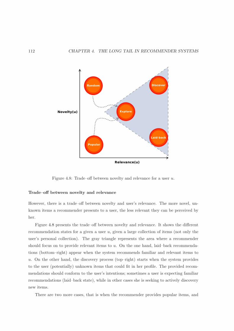
112 CHAPTER 4. THE LONG TAIL IN RECOMMENDER SYSTEMS
Figure 4.8: Trade–off between novelty and relevance for a user u.
Trade–off between novelty and relevance
However, there is a trade–off between novelty and user’s relevance. The more novel, un-
known items a recommender presents to a user, the less relevant they can be perceived by
her.
Figure 4.8 presents the trade–off between novelty and relevance. It shows the different
recommendation states for a given a user u, given a large collection of items (not only the
user’s personal collection). The gray triangle represents the area where a recommender
should focus on to provide relevant items to u. On the one hand, laid–back recommenda-
tions (bottom–right) appear when the system recommends familiar and relevant items to
u. On the other hand, the discovery process (top–right) starts when the system provides
to the user (potentially) unknown items that could fit in her profile. The provided recom-
mendations should conform to the user’s intentions; sometimes a user is expecting familiar
recommendations (laid–back state), while in other cases she is seeking to actively discovery
new items.
There are two more cases, that is when the recommender provides popular items, and
4.6. NOVELTY, FAMILIARITY AND RELEVANCE 113
when it provides random ones. This can happen when there is not enough information
about the user (e.g. the user cold–start problem). In this case, the system can recommend
popular items (bottom–left). Popular items are expected to be somehow familiar to the
user, but not necessarily relevant to her. The other situation is when the system provides
random recommendations to u (top–left). This case is similar to a shuffle playlist generator,
with the difference that in our case the items’ catalog is much bigger than the personal
music collection of u. Thus, there is less chances that user u might like any of the random
recommendations, as they are not personalised at all.
4.6.2 Related work
Serendipity and novelty are relevant aspects in the recommendation workflow (McNee et al.,
2006). Indeed, there is some related work that explicitly addresses these aspects. For
instance, five measures to capture redundancy are presented in (Zhang et al., 2002). These
measures allow one to infer whether an item—that is considered relevant—contains any
novel information to the user. Yang and Li (2005) defines novelty in terms of the user
knowledge and her degree of interest in a given item. In Weng et al. (2007), Weng et.
al propose a way to improve the quality and novelty of the recommendations by means
of a topic taxonomy-based recommender, and hot topic detection using association rules.
Other proposals include disregarding items if they are too similar to other items that the
user has already seen (Billsus and Pazzani, 2000), or simple metrics to measure novelty and
serendipity based on the average popularity of the recommended items Ziegler et al. (2005).
Even though all these approaches focus on providing novel and serendipitous recommen-
dations, there is no framework that consistently evaluates the provided recommendations.
Thus, there is a need to design evaluation metrics to deal with the effectiveness of novel
recommendations, not only measuring prediction accuracy, but taking into account other
aspects such as usefulness and quality (Herlocker et al., 2004; Adomavicius and Tuzhilin,
2005). Novelty metrics should look at how well a recommender system made a user aware of
previously unknown items, as well as to what extent users accept the new recommendations
(Herlocker et al., 2004).
Generally speaking, the most popular items in the collection are the ones with higher
probability that a given user will recognise, or be broadly familiar with. Likewise, one
can assume that items with less interaction—rating, purchasing, previewing—within the
community of users are more likely to be unknown (Ziegler et al., 2005). In this sense,

114 CHAPTER 4. THE LONG TAIL IN RECOMMENDER SYSTEMS
the Long Tail of the items’ catalog (Anderson, 2006) assists us in deciding how novel or
familiar an item could be. Yet, a recommender system must predict whether an item could
be relevant, and then be recommended, to a user.
4.7 Summary
Effective recommendation systems should promote novel and relevant material (non–obvious
recommendations), taken primarily from the tail of a popularity distribution. In this sense,
the Long Tail can be described in terms of niche markets’ economics, but also by describing
the item popularity curve. We use the latter definition —the Long Tail model, F (x)—
to describe the cumulative distribution of the curve. In the music field, the F (x) model
allows us to define artist popularity, and her location in the curve (head, mid or tail region).
Hence, F (x) denotes the shared knowledge about an artist, by a community of listeners.
From this common knowledge, we can derive whether an artist can be novel and relevant
to a given user profile.
Our results show that music listening habits follow the hit–driven (or mainstream)
paradigm. 0.28% (737 out of 260,525) of the artists account for the 50% of total playcounts.
The best fit (in the log–log plot) for the music Long Tail is a log–normal distribution.
A log–normal distribution concentrates most of the information in the the head region.
Even though we use playcounts and not total sales to populate the curve, this finding
unveils Anderson’s theory about the economics and monetisation in the Long Tail. Despite
Anderson’s failure or success theory, the main idea still is an interesting way to explain the
changes the web has provoked, in terms of the availability of all kind of products —from
hits to niches.
One of the goals of a recommender should be to promote the tail of the curve by providing
relevant, personalised novel recommendations to its users. That is, to smoothly interconnect
the head and mid regions with the tail, so the recommendations can drive interest from one
to the other. Figure 4.9 presents this idea. It depicts a 3D representation of the Long Tail;
showing the item popularity curve, a user profile example (denoted by her preferred items,
in gray colour), and the similarities among the items. The set of candidate items to be
recommended to the user are shown (in violet) and its height denotes the relevance for the
user. Candidate items located in the tail part are considered more novel —and, potentially
relevant— than the ones in the head region.

4.7. SUMMARY 115
Figure 4.9: (best seen in colour) A 3D representation of the Long Tail. It adds anotherdimension; the similarities among the items, including the representation of a user profile(in gray). The set of candidate items to be recommended to the user are shown (in violet)and its height denotes the relevance for the user. Candidate items located in the tail partare considered more novel —and, potentially relevant— than the ones in the head region.
116 CHAPTER 4. THE LONG TAIL IN RECOMMENDER SYSTEMS
Links with the following chapters
In this chapter we have presented the basics for novelty detection in a recommender sys-
tem, using the popularity information and its Long Tail shape. The next step is to evaluate
these types of recommendations. We can foresee two different ways to evaluate novel rec-
ommendations, and these are related with (i) exploring the available (and usually, very
large) item catalog, and (ii) filtering new incoming items. In this Thesis we mainly focus
on the former case, and we present two complementary evaluation methods. On the one
hand, network–centric evaluation method (presented in chapter 6) focuses on analysing
the items’ similarity graph, created using any item–based recommendation algorithm. The
aim is to detect whether the intrinsic topology of the items’ network has any pathology that
hinders novel recommendations, promoting the most popular items. On the other hand,
a user–centric evaluation aims at measuring the perceived quality of novel recommen-
dations. This evaluation is presented in chapter 7. Yet, before presenting the evaluation
results we introduce, in chapter 5, the metrics that we use.
Chapter 5
Evaluation metrics
This chapter presents the different evaluation methods for a recommender system. We
introduce the existing metrics, as well as the pros and cons of each method. This chapter
is the background for the following chapters 6 and 7, where the proposed metrics are used
in real, large size, recommendation datasets.
5.1 Evaluation strategies
We classify the evaluation of recommender algorithms in three groups; system–, network–,
and user–centric.
• System–centric evaluation measures how accurate the system can predict the actual
values that user have previously assigned. This approach has been extensively used
in collaborative filtering, with explicit feedback (e.g. ratings).
• Network–centric evaluation aims at measuring the topology of the item (or user)
network similarity. It uses metrics from complex network analysis (CNA).
• User–centric evaluation focuses on the user’s perceived quality and usefulness of the
recommendations.
The following sections are devoted to explain each evaluation method.
117
118 CHAPTER 5. EVALUATION METRICS
5.2 System–centric evaluation
As of today, system–centric evaluation has been largely studied. The most common ap-
proaches are based on the leave–n–out method (Breese et al., 1998), that resembles to the
classic n–fold cross validation. Given a dataset where a user has implicitly or explicitly
interacted with (via ratings, purchases, downloads, previews, etc.), split the dataset in
two—usually disjunct—sets: training and test. The evaluation of the accuracy is based
only on a user’s dataset, so the rest of the items are ignored. Figure 5.1 presents the
method.
The evaluation process includes, then, several metrics such as: predictive accuracy
(Mean Absolute Error, Root Mean Square Error), decision based (Mean Average Preci-
sion, Recall, F–measure, and ROC), and rank based metrics (Spearman’s ρ, Kendall–τ ,
and half–life utility) (Herlocker et al., 2004). The main problem, though, is to develop
evaluation metrics to deal with the effectiveness of the recommendations. That is, not only
measuring prediction accuracy, but taking into account other aspects such as usefulness and
quality (Adomavicius and Tuzhilin, 2005).
5.2.1 Predictive–based metrics
Predictive metrics aim at comparing the predicted values against the actual values. The
result is the average over the deviations.
Mean Absolute Error (MAE)
Mean Absolute Error (MAE) measures the deviation between the predicted value and the
real value.
MAE =1
n
n∑
i=1
∣
∣
∣Ri − Ri
∣
∣
∣, (5.1)
where Ri is the predicted value and Ri the true value.
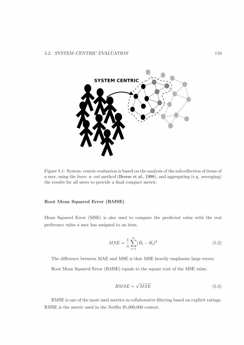
5.2. SYSTEM–CENTRIC EVALUATION 119
Figure 5.1: System–centric evaluation is based on the analysis of the subcollection of items ofa user, using the leave–n–out method (Breese et al., 1998), and aggregating (e.g. averaging)the results for all users to provide a final compact metric.
Root Mean Squared Error (RMSE)
Mean Squared Error (MSE) is also used to compare the predicted value with the real
preference value a user has assigned to an item.
MSE =1
n
n∑
i=1
(Ri − Ri)2 (5.2)
The difference between MAE and MSE is that MSE heavily emphasise large errors.
Root Mean Squared Error (RMSE) equals to the square root of the MSE value.
RMSE =√
MSE (5.3)
RMSE is one of the most used metrics in collaborative filtering based on explicit ratings.
RMSE is the metric used in the Netflix $1,000,000 contest.
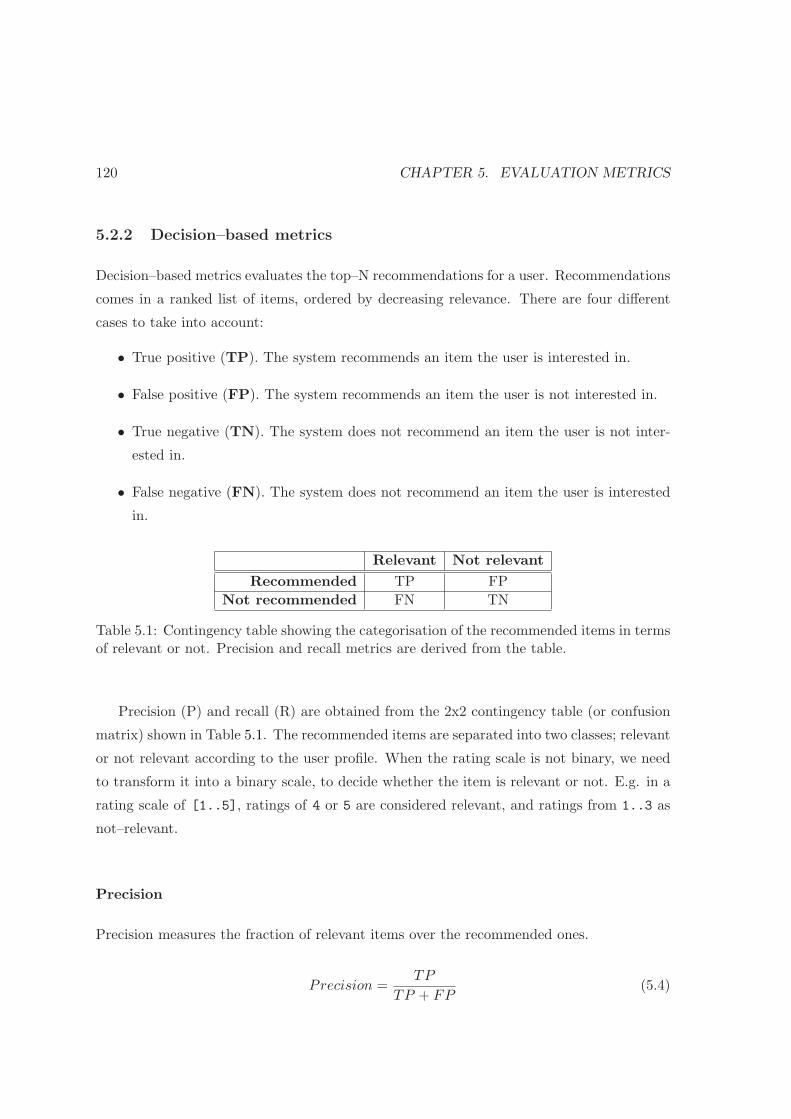
120 CHAPTER 5. EVALUATION METRICS
5.2.2 Decision–based metrics
Decision–based metrics evaluates the top–N recommendations for a user. Recommendations
comes in a ranked list of items, ordered by decreasing relevance. There are four different
cases to take into account:
• True positive (TP). The system recommends an item the user is interested in.
• False positive (FP). The system recommends an item the user is not interested in.
• True negative (TN). The system does not recommend an item the user is not inter-
ested in.
• False negative (FN). The system does not recommend an item the user is interested
in.
Relevant Not relevant
Recommended TP FP
Not recommended FN TN
Table 5.1: Contingency table showing the categorisation of the recommended items in termsof relevant or not. Precision and recall metrics are derived from the table.
Precision (P) and recall (R) are obtained from the 2x2 contingency table (or confusion
matrix) shown in Table 5.1. The recommended items are separated into two classes; relevant
or not relevant according to the user profile. When the rating scale is not binary, we need
to transform it into a binary scale, to decide whether the item is relevant or not. E.g. in a
rating scale of [1..5], ratings of 4 or 5 are considered relevant, and ratings from 1..3 as
not–relevant.
Precision
Precision measures the fraction of relevant items over the recommended ones.
Precision =TP
TP + FP(5.4)
5.2. SYSTEM–CENTRIC EVALUATION 121
Recall
The recall measures the coverage of the recommended items, and is defined as:
Recall =TP
TP + FN(5.5)
Recall is also known as sensitivity, true positive rate (TPR), or hit–rate.
F–measure
F–measure combines P and R results, using the weighted harmonic mean. The general
formula (for a non-negative real β) is:
Fβ =(1 + β2) · (precision · recall)
(β2 · precision + recall)(5.6)
Two common F–measures are F1 and F2. In F1 recall and precision are evenly weighted,
and F2 weights recall twice as much as precision.
Accuracy
Accuracy is the simplest way to evaluate the predicted recommendations. Accuracy mea-
sures the ratio of correct predictions versus the total number of items evaluated. Accuracy
is also obtained from the 2x2 contingency table.
Accuracy =TP + TN
TP + FP + TN + FN(5.7)
Receiver Operating Characteristic (ROC) curve
Receiver Operating Characteristic (ROC) curve measures the selection of high–quality items
from the recommended list. ROC measures the trade–off between hit–rates (TPR) and
false–alarm rates (or false positive rates, FPR). Hit–rate, or True Positive Rate, is defined
as TPR = Recall. False positive rate (FPR) equals to FPR = FPFP+TN
ROC can visualise the trade–off between TPR and FPR. The random curve assigns a
probability of 50% to each of the two classes (recommended, not recommended). The area
under the curve (AUC) is a measure that summarises a ROC result. A random curve has
an AUC of 0.5. The closer the AUC to 1, the better.

122 CHAPTER 5. EVALUATION METRICS
The main drawback of decision–based metrics is that do not take into account the
ranking of the recommended items. Thus, item at top–1 has the same relevance as an item
at top–20. To avoid this problem, we can use rank–based metrics.
5.2.3 Rank–based metrics
Rank–based metrics use the item position in the predicted list of recommendations. The
idea is that top items should be considered more relevant than the items in the bottom of
the recommendation list.
Spearman’s rho (ρ)
Spearman’s ρ computes the rank–based Pearson correlation of two ranked lists. It compares
the predicted list with the user profile information (e.g. the ground truth data), and it takes
into account the ranking position of each recommended item. Spearman’s ρ is defined as:
ρ = 1 − 6∑
d2i
n(n2 − 1)(5.8)
where di = xi − yi denotes the difference between the ranks of corresponding values Ri and
Ri.
Kendall–tau (τ)
Kendall–τ also compares the recommended list with the user’s list of items (e.g. the ground
truth data). Kendall–τ rank correlation coefficient is defined as:
τ =nc − nd
12n(n − 1)
(5.9)
where nc is the number of concordant pairs, and nd is the number of discordant pairs
in the data set.
5.2. SYSTEM–CENTRIC EVALUATION 123
Average Reciprocal Hit–Rate
Average Reciprocal Hit–Rate (ARHR) was first used in (Karypis, 2001). ARHR rewards
each hit based on where is located in the top-N list. ARHR is defined as:
ARHR =1
n
h∑
i=1
1
pi(5.10)
where h is the number of hits that occurred at positions p1, p2, ..., ph within the top-N lists.
Hits that occur earlier in the top-N lists are weighted higher than hits that occur later in
the list. ARHR resembles to the Mean Reciprocal Rank metric from IR.
5.2.4 Other metrics
Half–life utility
Half–life utility metric attempts to evaluate the utility of the predicted list of items (Breese et al.,
1998). The utility is defined as the deviation between a user’s rating and the default rating
for an item. So, half–life utility can be used in algorithms that are based on user explicit
feedback, such as ratings. Breese et al. (1998) describe the likelihood that a user will view
each successive item in the ranked list with an exponential decay function. The strength of
the decay is described by a half–life parameter α. Half–life utility is defined as:
HL =∑
i
max(Ru,i − di, 0)
2(i − 1)/(α − 1)(5.11)
where, Ru,i represents the rating of user u on item i of the ranked list, d is the default
rating for item i, and α is the half-life.
Normalised distance–based performance
Normalised distance-based performance (NDPM) was introduced in (Balabanovic and Shoham,
1997) to evaluate their collaborative filtering recommender system, named FAB.
NPDM is a normalised distance (to range [0..1]), between the user’s classification for
a set of documents and the system’s classification for the same documents (Yao, 1995). In
recommender systems, NDPM measures the difference between the user’s and the system’s
124 CHAPTER 5. EVALUATION METRICS
choices. NDPM is defined as:
NDPM =2C(−) + C(u)
2C(i)(5.12)
where C(−) is number of mismatched preference relations between the system and user
rankings, C(u) is number of compatible preference relations, and C(i) is the total number
of preferred relationships in the user’s ranking.
A/B testing
In A/B testing, the system unleash two different versions of an algorithm (or two completely
different algorithms), and see which one performs the best. The performance is measured
by the impact the new algorithm has on the visitors’ behaviour, compared with the baseline
algorithm. A/B testing became very popular on the Web, because it is easy to create
different webpage versions, and show them to visitors. One of the first examples that used
A/B test was Amazon.com.
The evaluation is performed by only changing a few aspects between the two versions.
Once a baseline is established, the system starts optimising the algorithm by making one
change at a time, and evaluating the results and impact with real visitors of the page.
5.2.5 Limitations
The main limitation of system–centric evaluation is the set of items that can evaluate.
System–centric evaluation cannot avoid the selection bias of the dataset. Users do not rate
all the items they receive, but rather they select the ones to rate. The observations a system–
centric approach can evaluate is a skewed, narrowed and unrepresentative population of the
whole collection of items. That is, for a given user, the system–centric approach only
evaluates the items the user has interacted with, neglecting the rest of the collection. The
same procedure is applied for the rest of the users, and the final metrics are averaged over
all the users.
These metrics present some drawbacks that are intrinsic to the approach used:
• The coverage of the recommended items cannot be measured. The collection of items
used in the evaluation is limited to the set of items that a user has interacted with.
• The novelty of the recommendations cannot be measured. System–centric evaluates
the set of items a user has interacted with. Thus, it cannot evaluate the items that
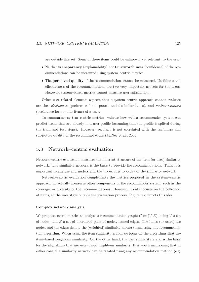
5.3. NETWORK–CENTRIC EVALUATION 125
are outside this set. Some of these items could be unknown, yet relevant, to the user.
• Neither transparency (explainability) nor trustworthiness (confidence) of the rec-
ommendations can be measured using system–centric metrics.
• The perceived quality of the recommendations cannot be measured. Usefulness and
effectiveness of the recommendations are two very important aspects for the users.
However, system–based metrics cannot measure user satisfaction.
Other user–related elements aspects that a system–centric approach cannot evaluate
are the eclecticness (preference for disparate and dissimilar items), and mainstreamness
(preference for popular items) of a user.
To summarise, system–centric metrics evaluate how well a recommender system can
predict items that are already in a user profile (assuming that the profile is splited during
the train and test steps). However, accuracy is not correlated with the usefulness and
subjective quality of the recommendations (McNee et al., 2006).
5.3 Network–centric evaluation
Network–centric evaluation measures the inherent structure of the item (or user) similarity
network. The similarity network is the basis to provide the recommendations. Thus, it is
important to analyse and understand the underlying topology of the similarity network.
Network–centric evaluation complements the metrics proposed in the system–centric
approach. It actually measures other components of the recommender system, such as the
coverage, or diversity of the recommendations. However, it only focuses on the collection
of items, so the user stays outside the evaluation process. Figure 5.2 depicts this idea.
Complex network analysis
We propose several metrics to analyse a recommendation graph; G := (V, E), being V a set
of nodes, and E a set of unordered pairs of nodes, named edges. The items (or users) are
nodes, and the edges denote the (weighted) similarity among them, using any recommenda-
tion algorithm. When using the item similarity graph, we focus on the algorithms that use
item–based neighbour similarity. On the other hand, the user similarity graph is the basis
for the algorithms that use user–based neighbour similarity. It is worth mentioning that in
either case, the similarity network can be created using any recommendation method (e.g.
126 CHAPTER 5. EVALUATION METRICS
Figure 5.2: Network–centric evaluation determines the underlying topology of the item (oruser) similarity network.
collaborative filtering, content–based, hybrid, etc.). All the proposed metrics are derived
from Complex Network and Social Network analysis.
5.3.1 Navigation
Average shortest path
The average shortest path (or mean geodesic length) measures the distance between two
vertices i and j. They are connected if one can go from i to j following the edges in the
graph. The path from i to j may not be unique. The minimum path distance (or geodesic
path) is the shortest path distance from i to j, dij . The average shortest path in the network
is:
〈d〉 =1
12n(n + 1)
∑
i,j∈V,i6=j
dij (5.13)
In a random graph, the average path approximates to:
〈dr〉 ∼logN
log 〈k〉 , (5.14)
where N = |V |, and 〈k〉 denotes the mean degree of all the nodes.
The longest path in the network is called its diameter (D). In a recommender system,
average shortest path and diameter inform us about the global navigation through the
network of items.
5.3. NETWORK–CENTRIC EVALUATION 127
Giant component
The strong giant component, SGC, of a network is the set of vertices that are connected
via one or more geodesics, and are disconnected from all other vertices. Typically, networks
have one large component that contains most of the vertices. It is measured as the %
of nodes that includes the giant component. In a recommender system, SGC informs us
about the catalog coverage, that is the total percentage of available items the recommender
recommends to users (Herlocker et al., 2004).
5.3.2 Connectivity
Degree distribution
The degree distribution, pk, is the number of vertices with degree k:
pk =∑
v∈V | deg(v)=k
1, (5.15)
where v is a vertex, and deg(v) its degree. More frequently, the cumulative degree
distribution (the fraction of vertices having degree k or larger), is plotted:
Pc(k) =∞
∑
k′=k
pk′ (5.16)
A cumulative plot avoids fluctuations at the tail of the distribution and facilitates the
computation of the power coefficient γ, if the network follows a power law. Pc(k) is, then,
usually plotted as the complementary cumulative distribution function (ccdf ). The com-
plementary cumulative distribution function, Fc(x), is defined as:
Fc(x) = P[X > x] = 1 − F (x) (5.17)
where F (x) is the cumulative distribution function (cdf ):
F (x) = P[X ≤ x] (5.18)
F (x) can be regarded as the proportion of the population whose value is less than x.
Thus, Pc(k), derived from Fc(x), denotes the fraction of nodes with a degree greater than
or equal to k.
128 CHAPTER 5. EVALUATION METRICS
In a directed graph, that is when a recommender algorithm only computes the top–n
most similar items, P (kin) and P (kout), the cumulative incoming (outcoming) degree dis-
tribution, are more informative. Complementary cumulative indegree distribution, Pc(kin),
detects whether a recommendation network has some nodes that act as hubs. That is, that
they have a large amount of attached links. This clearly affects the recommendations and
navigability of the network.
Also, the shape of the curve helps us to identify the network’s topology. Regular net-
works have a constant distribution, “random networks” have a Poisson degree distribution
(Erdos and Reyi, 1959) meaning that there are no hubs, and “scale–free networks” follow a
power–law distribution in the cumulative degree distribution (Barabasi and Albert, 1999),
so there are a few hubs that control the network. It is worth noting that many real–world
networks, including the world wide web linking structure, are known to show a right–skewed
distribution (often a power law P (k) ∝ k−γ with 2 < γ < 3).
Degree–degree correlation
Another metric used is the degree correlation. It is equal to the average nearest–
neighbour degree, knn, as a function of k:
knn(k) =∞
∑
k′=0
k′p(k′|k), (5.19)
where p(k′|k) is the fraction of edges that are attached to a vertex of degree k whose
other ends are attached to vertex of degree k′. Thus, knn(k) is the mean degree of the
vertices we find by following a link emanating from a vertex of degree k.
A closely related concept is the degree–degree correlation coefficient, also known as
assortative mixing, which is the Pearson r correlation coefficient for degrees of vertices
at either end of a link. A monotonically increasing (decreasing) knn means that high–
degree vertices are connected to other high–degree (low–degree) vertices, resulting in a
positive (negative) value of r (Newman, 2002). In recommender systems, it measures to
which extent nodes are connected preferentially to other nodes with similar characteristics.

5.3. NETWORK–CENTRIC EVALUATION 129
Mixing patterns
We can generalise the vertex assortative mixing to any network pattern. Assortative mixing
has an impact on the structural properties of the network. Mixing by a discrete character-
istic of the network (e.g. race, language, or age in social networks) tend to separate the
network into different communities. In social networks, this is also known as homophily.
We use the formula defined in (Newman, 2003a) to compute mixing patterns for discrete
attributes. Let E be an N×N matrix, where Eij contains the number of edges in the network
that connect a vertex of type i to one of type j (Eij = Eji in undirected networks). The
normalised mixing matrix is defined as:
e =E
‖ E ‖ (5.20)
where ‖ x ‖ means the sum of all elements in the matrix x. Mixing characteristics is
measured in the normalised matrix e. Matrix e satisfies the following sum rules:
∑
ij
eij = 1, (5.21)
∑
j
eij = ai, (5.22)
∑
i
eij = bj , (5.23)
where ai and bi are the fraction of each type of an end of an edge that is attached to
nodes of type i. The assortative mixing coefficient r is defined as:
r =
∑
i eii −∑
i aibi
1 − ∑
i aibi=
Tr(e)− ‖ e2 ‖1− ‖ e2 ‖ (5.24)
This quantity equals to 0 in a randomly mixed network, and 1 in a perfectly mixed
network. Dissassortative networks have a negative r value, whilst assortative networks have
a positive one.
5.3.3 Clustering
Clustering is a fundamental facet to describe the navigation in a network.
130 CHAPTER 5. EVALUATION METRICS
Local clustering coefficient
The local clustering coefficient, Ci, of a node i represents the probability of its neighbours
to be connected within each other.
Ci =2|Ei|
ki(ki − 1), (5.25)
where Ei is the set of existing edges that are direct neighbours of i, and ki the degree
of i. Ci denotes, then, the portion of actual edges of i from the potential number of
total edges. 〈C〉 is defined as the average over the local measure Ci, 〈C〉 = 1n
∑ni=1 Ci
(Watts and Strogatz, 1998).
Global clustering coefficient
The global clustering coefficient is a sign of how cliquish (tightly knit) a network is. It
estimates the conditional probability that two neighbouring vertices of a given vertex are
neighbours themselves. The global clustering coefficient, C, It is quantified by the abun-
dance of triangles in a network, where a triangle is formed when three vertices are all linked
to one another.
C =3 × number of triangles
number of connected triples. (5.26)
Here, a connected triple means a pair of vertices connected via another vertex. Since
a triangle contains three triples, C is equal to the probability that two neighbours of a
vertex are connected as well. For random graphs, the clustering coefficient is defined as
Cr ∼ 〈k〉 /N . Typically, real networks have a higher clustering coefficient than Cr.
Some real–world networks are known to show a behaviour of C(k) ∝ k−1, usually
attributed to the hierarchical nature of the network (Ravasz and Barabasi, 2003). This
behaviour has been found in metabolic networks, as well as in the WWW, and movie actor
networks (Ravasz et al., 2002). The reasons for modular organisation in these networks
relate, respectively, to the function in metabolic interaction networks, the topology of In-
ternet, and the social activities in social networks.
5.3. NETWORK–CENTRIC EVALUATION 131
5.3.4 Related work in music information retrieval
During the last few years, complex network analysis has been applied to music information
retrieval, and music recommendation in particular. In (Cano et al., 2006), we compared
different music recommendation algorithms based on the network topology. The results
show that social based recommenders present a scale–free network topology, whereas human
expert–based controlled networks does not.
An empirical study of the evolution of a social network constructed under the influence
of musical tastes, based on playlist co-occurrence, appears in (Martin-Buldu et al., 2007).
The analysis of collaboration among contemporary musicians, in which two musicians are
connected if they have performed in or produced an album together, appears in (Park et al.,
2007). Anglade et al. (2007a) present a user clustering algorithm that exploits the topology
of a user–based similarity network.
Aucouturier and Pachet (2008) present a network of similar songs based on timbre sim-
ilarity. Interestingly enough, the network is scale–free, thus a few songs appear in almost
any list of similar tracks. This has some problems when generating automatic playlists.
Jacobson and Sandler (2008) present an analysis of the Myspace social network, and con-
clude that artists tend to form on-line communities with artists of the same musical genre.
Lambiotte and Ausloos (2005) present a method of clustering genres, by analysing cor-
relations between them. The analysis is based on the users’ listening habits, gathered from
last.fm. From the 〈user, artist, plays〉 triples the authors compute genre similarity based
on the percolation idea in complex networks, and also visualise a music genre cartography,
using a tree representation.
5.3.5 Limitations
The main limitation of the network–centric approach is that users remain outside the eval-
uation process. There is no user intervention, not even the information of a user profile is
taken into account in the evaluation. The main drawbacks of network–centric approach are:
• Accuracy of the recommendations cannot be measured. In the network–centric ap-
proach there is no way to evaluate “how well” the algorithm is predicting the items
already in a user’s profile.
• Neither transparency (explainability) nor trustworthiness (confidence) of the rec-
ommendations can be measured.
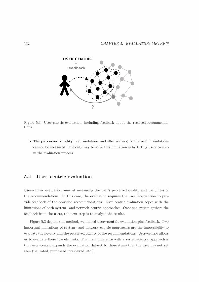
132 CHAPTER 5. EVALUATION METRICS
Figure 5.3: User–centric evaluation, including feedback about the received recommenda-tions.
• The perceived quality (i.e. usefulness and effectiveness) of the recommendations
cannot be measured. The only way to solve this limitation is by letting users to step
in the evaluation process.
5.4 User–centric evaluation
User–centric evaluation aims at measuring the user’s perceived quality and usefulness of
the recommendations. In this case, the evaluation requires the user intervention to pro-
vide feedback of the provided recommendations. User–centric evaluation copes with the
limitations of both system– and network–centric approaches. Once the system gathers the
feedback from the users, the next step is to analyse the results.
Figure 5.3 depicts this method, we named user–centric evaluation plus feedback. Two
important limitations of system– and network–centric approaches are the impossibility to
evaluate the novelty and the perceived quality of the recommendations. User–centric allows
us to evaluate these two elements. The main difference with a system–centric approach is
that user–centric expands the evaluation dataset to those items that the user has not yet
seen (i.e. rated, purchased, previewed, etc.).

5.4. USER–CENTRIC EVALUATION 133
5.4.1 Metrics
In the user–centric approach, the recommender system presents relevant items (from outside
the user’s dataset), and asks user for feedback. Feedback gathering can be done in two ways:
implicitly or explicitly. Measuring implicit feedback includes, for instance, the time spent
in the item’s webpage, purchasing or not the item, previewing it, etc. Explicit feedback is
based on two related questions; (i) whether the user already knew the item (novelty), and
(ii) whether she likes it or not (perceived quality). Obviously, it requires an extra effort
from the users, but at the same time it provides unequivocal information about the intended
dimensions (which in the case of implicit measures could be ambiguous or inaccurate).
Perceived quality
The easiest way to measure the perceived quality of the recommended items is by explicitly
asking to the users. Users must examine the recommended items and validate, to some
extent, whether they like the items or not (Herlocker et al., 2004). In this sense, a user
needs the maximum information about the item (e.g. metadata information, a preview,
etc.), and the reasons why the item was recommended, if possible. Then, the user has to
rate the quality of each recommended item (e.g. in a rating scale of [1..5]), or the quality
of the list as a whole. Last but not least, the user should be able to select those attributes
of the item that makes her feel that the novel item is relevant to her taste.
Novelty
To evaluate novel items we need, again, to ask to the users whether they recognise the
predicted item or not. Users have to examine the list of recommended items and express,
for each item, whether she previously knew the item or not.
Combining both aspects, perceived quality and novelty, allows the system to infer whe-
ther a user likes to receive and discover unknown items, or in contrast, she prefers to get
more conservative and familiar recommendations. Adding the transparency (explainability)
in the recommendations, the user can perceive the new items as of higher quality, as the
system can give an explanation of why this unknown item was recommended to the user.
All in all, the user’s intentions with regard novelty detection depends on the context and
the recommendation domain. Furthermore, it is expected that the intentions change over
time. For instance, a user is sometimes open to discovering new artists and songs, while

134 CHAPTER 5. EVALUATION METRICS
sometimes she just wants to listen to her favourites. Detecting these modes and acting
accordingly would increase user’s satisfaction with the system.
5.4.2 Limitations
The main limitation of the user–centric approach is the need of user intervention in the
evaluation process. Gathering feedback from the user can be tedious for some users (filling
surveys, rating items, providing feedback, etc.). In this sense, the system should ease and
minimise the user intervention, using (whenever is possible) an unintrusive way. On the
other hand, the main limitations from the two previous approaches (perceived quality and
novelty detection) are solved in this approach.
5.5 Summary
We classify the evaluation of recommender algorithms in: system–, network–, and user–
centric approaches. System–centric evaluation measures how accurately the recommender
system can predict the actual values that users have previously assigned. Network–centric
evaluation aims at measuring the topology of the item (or user) network similarity, and
it uses metrics from complex network analysis. Finally, user–centric evaluation focuses on
the user’s perceived quality and usefulness of the recommendations. Combining the three
methods we can cover all the facets of a recommender algorithm; the system–centric ap-
proach evaluates the performance accuracy of the algorithm, the network–centric approach
analyses the structure of the similarity network, and with the inclusion of the user inter-
vention we can measure the satisfaction about the recommendations they receive. Figure
5.4 depicts this idea. We can see that, when using the three evaluation approaches, all the
components are evaluated —algorithm accuracy, similarity network analysis, and feedback
from users.
Last but not least, Table 5.2 summarises the limitations of each approach. The table
presents some of the factors that affect the recommendations, and whether the approach can
evaluate it or not. Applying the three evaluation approaches, we can assess all the facets of
a recommender system, and also cope with the limitations of each evaluation approach.
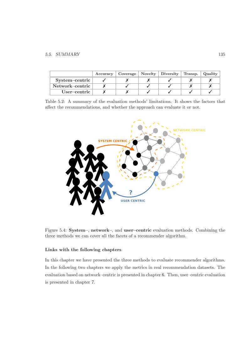
5.5. SUMMARY 135
Accuracy Coverage Novelty Diversity Transp. Quality
System–centric 3 7 7 3 7 7
Network–centric 7 3 3 3 7 7
User–centric 7 7 3 3 3 3
Table 5.2: A summary of the evaluation methods’ limitations. It shows the factors thataffect the recommendations, and whether the approach can evaluate it or not.
Figure 5.4: System–, network–, and user–centric evaluation methods. Combining thethree methods we can cover all the facets of a recommender algorithm.
Links with the following chapters
In this chapter we have presented the three methods to evaluate recommender algorithms.
In the following two chapters we apply the metrics in real recommendation datasets. The
evaluation based on network–centric is presented in chapter 6. Then, user–centric evaluation
is presented in chapter 7.

136 CHAPTER 5. EVALUATION METRICS
Chapter 6
Network–centric evaluation
In this chapter we present the network–centric evaluation approach. This method analy-
ses the similarity network, created using any recommendation algorithm. Network–centric
evaluation uses complex networks analysis to characterise the item collection. Also, we can
combine the results from the network analysis with the popularity of the items, using the
Long Tail model.
We perform several experiments in the music recommendation field. The first exper-
iment aims at evaluating the popularity effect using three music artists recommendation
approaches: collaborative filtering (CF), content–based audio similarity (CB), and human
expert–based resemblance. The second experiment compare two user networks created by
CF and CB derived from the users’ listening habits. In all the three experiments, we mea-
sure the popularity effect by contrasting the properties from the network with the Long Tail
information (e.g. are the hubs in the recommendation network the most popular items?
Or, are the most popular items connected with other popular items?).
6.1 Network analysis and the Long Tail model
Figure 6.1 presents the framework for the network–centric evaluation. It includes the simi-
larity network and the Long Tail of item popularity. This approach combines the analysis
of the similarity network with the Long Tail of popularity.
Once each item in the recommendation network is located in the head, mid, or tail part
(see section 4.3.2), the next step is to combine the similarity network with the Long Tail
information. Two main analysis are performed: first, we measure the similarity among
137
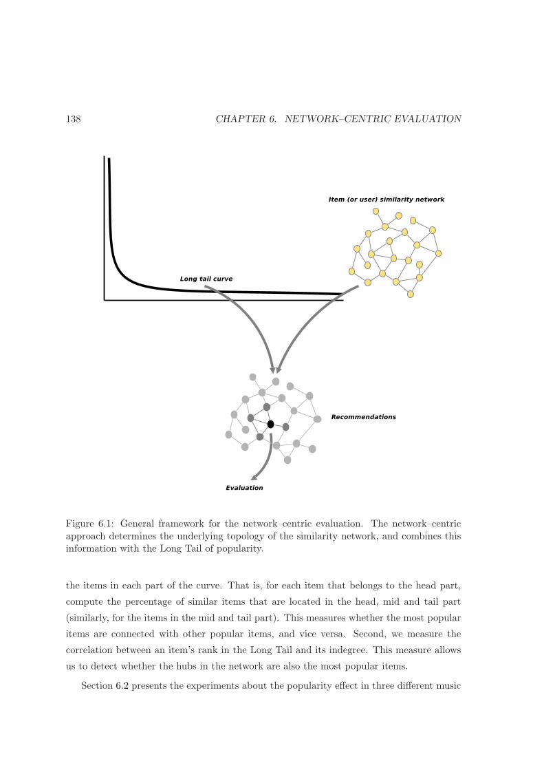
138 CHAPTER 6. NETWORK–CENTRIC EVALUATION
Figure 6.1: General framework for the network–centric evaluation. The network–centricapproach determines the underlying topology of the similarity network, and combines thisinformation with the Long Tail of popularity.
the items in each part of the curve. That is, for each item that belongs to the head part,
compute the percentage of similar items that are located in the head, mid and tail part
(similarly, for the items in the mid and tail part). This measures whether the most popular
items are connected with other popular items, and vice versa. Second, we measure the
correlation between an item’s rank in the Long Tail and its indegree. This measure allows
us to detect whether the hubs in the network are also the most popular items.
Section 6.2 presents the experiments about the popularity effect in three different music

6.2. ARTIST NETWORK ANALYSIS 139
artists recommendation algorithms: collaborative filtering (CF) from last.fm, content–based
audio filtering (CB), and expert–based recommendations (EX)from Allmusic.com (AMG)
musicologists. Then, section 6.3 compares two user similarity networks created using col-
laborative filtering (CF) again from last.fm, and a user similarity network derived from the
users’ listening habits. In this case, we use content–based audio similarity (CB) to create
the links among users.
6.2 Artist network analysis
We aim to evaluate three artist similarity networks: collaborative filtering (CF), content–
based audio similarity (CB), and human expert–based resemblance. Also, we analyse the
popularity effect for each recommendation network. We measure the popularity effect by
contrasting the properties from the network with the Long Tail information of the catalog.
6.2.1 Datasets
Social–based, collaborative filtering network
Artist similarity is gathered from last.fm, using Audioscrobbler web services1, and select-
ing the top–20 similar artists. Last.fm has a strong social component, and their recom-
mendations are based on a combination of an item–based collaborative filtering, plus the
information derived from social tagging. We denote this network as CF .
Human expert–based network
We have gathered human–based expert recommendations from All Music Guide (AMG)2.
AMG makes use of professional editors to interconnect artists, according to several aspects,
such as: influenced by, followers of, similar artists, performed songs by, etc. In order to
create an homogeneous network, we only use the similar artists links. We denote this
network as EX.
Table 6.1 shows the number of nodes and edges, for each network.
1http://www.audioscrobbler.net/data/webservices/2http://www.allmusic.com
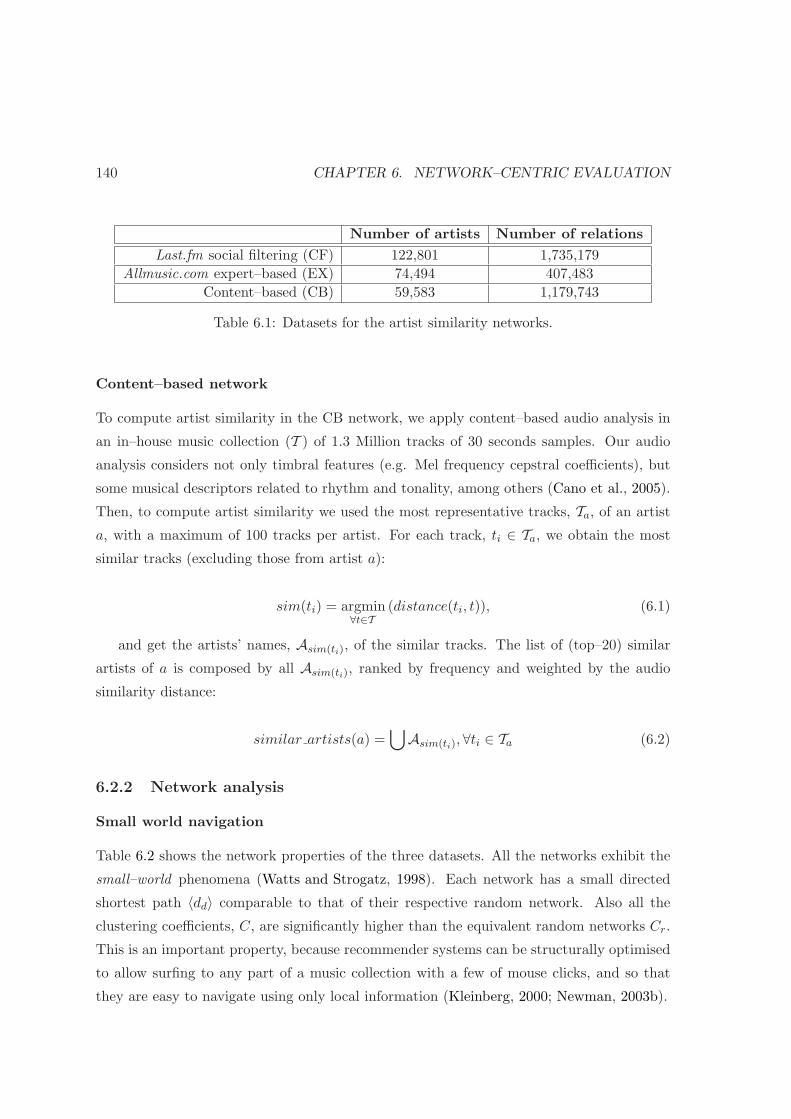
140 CHAPTER 6. NETWORK–CENTRIC EVALUATION
Number of artists Number of relations
Last.fm social filtering (CF) 122,801 1,735,179
Allmusic.com expert–based (EX) 74,494 407,483
Content–based (CB) 59,583 1,179,743
Table 6.1: Datasets for the artist similarity networks.
Content–based network
To compute artist similarity in the CB network, we apply content–based audio analysis in
an in–house music collection (T ) of 1.3 Million tracks of 30 seconds samples. Our audio
analysis considers not only timbral features (e.g. Mel frequency cepstral coefficients), but
some musical descriptors related to rhythm and tonality, among others (Cano et al., 2005).
Then, to compute artist similarity we used the most representative tracks, Ta, of an artist
a, with a maximum of 100 tracks per artist. For each track, ti ∈ Ta, we obtain the most
similar tracks (excluding those from artist a):
sim(ti) = argmin∀t∈T
(distance(ti, t)), (6.1)
and get the artists’ names, Asim(ti), of the similar tracks. The list of (top–20) similar
artists of a is composed by all Asim(ti), ranked by frequency and weighted by the audio
similarity distance:
similar artists(a) =⋃
Asim(ti),∀ti ∈ Ta (6.2)
6.2.2 Network analysis
Small world navigation
Table 6.2 shows the network properties of the three datasets. All the networks exhibit the
small–world phenomena (Watts and Strogatz, 1998). Each network has a small directed
shortest path 〈dd〉 comparable to that of their respective random network. Also all the
clustering coefficients, C, are significantly higher than the equivalent random networks Cr.
This is an important property, because recommender systems can be structurally optimised
to allow surfing to any part of a music collection with a few of mouse clicks, and so that
they are easy to navigate using only local information (Kleinberg, 2000; Newman, 2003b).
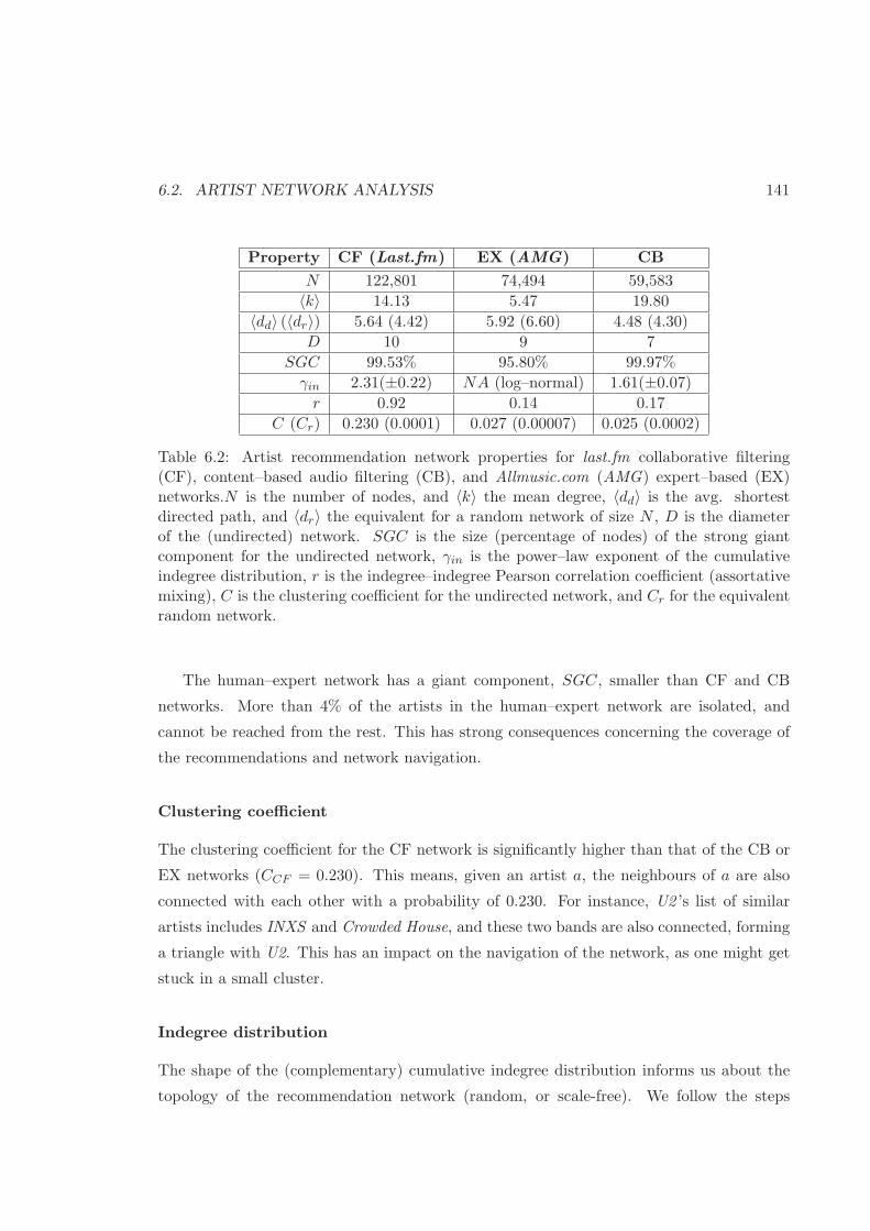
6.2. ARTIST NETWORK ANALYSIS 141
Property CF (Last.fm) EX (AMG) CB
N 122,801 74,494 59,583
〈k〉 14.13 5.47 19.80
〈dd〉 (〈dr〉) 5.64 (4.42) 5.92 (6.60) 4.48 (4.30)
D 10 9 7
SGC 99.53% 95.80% 99.97%
γin 2.31(±0.22) NA (log–normal) 1.61(±0.07)
r 0.92 0.14 0.17
C (Cr) 0.230 (0.0001) 0.027 (0.00007) 0.025 (0.0002)
Table 6.2: Artist recommendation network properties for last.fm collaborative filtering(CF), content–based audio filtering (CB), and Allmusic.com (AMG) expert–based (EX)networks.N is the number of nodes, and 〈k〉 the mean degree, 〈dd〉 is the avg. shortestdirected path, and 〈dr〉 the equivalent for a random network of size N , D is the diameterof the (undirected) network. SGC is the size (percentage of nodes) of the strong giantcomponent for the undirected network, γin is the power–law exponent of the cumulativeindegree distribution, r is the indegree–indegree Pearson correlation coefficient (assortativemixing), C is the clustering coefficient for the undirected network, and Cr for the equivalentrandom network.
The human–expert network has a giant component, SGC, smaller than CF and CB
networks. More than 4% of the artists in the human–expert network are isolated, and
cannot be reached from the rest. This has strong consequences concerning the coverage of
the recommendations and network navigation.
Clustering coefficient
The clustering coefficient for the CF network is significantly higher than that of the CB or
EX networks (CCF = 0.230). This means, given an artist a, the neighbours of a are also
connected with each other with a probability of 0.230. For instance, U2 ’s list of similar
artists includes INXS and Crowded House, and these two bands are also connected, forming
a triangle with U2. This has an impact on the navigation of the network, as one might get
stuck in a small cluster.
Indegree distribution
The shape of the (complementary) cumulative indegree distribution informs us about the
topology of the recommendation network (random, or scale-free). We follow the steps

142 CHAPTER 6. NETWORK–CENTRIC EVALUATION
Figure 6.2: Cumulative indegree distribution for the three artist networks.
defined in section 4.4 to decide whether or not the indegree distribution follows a power–
law (and, thus, it is a scale-free network).
power–law power–law + cut-off log–normal support forp LLR p xcutoff LLR p power–law
CF 0.9 -165.48 0.00 ≈ 102 -25.15 0.00 with exp. decay cut–offExpert 0.43 -41.05 0.00 ≈ 66 -5.86 0.00 moderate, with cut–off
CB 0.12 -905.96 0.00 ≈ 326 -99.68 0.00 moderate, with cut–off
Table 6.3: Model selection for the indegree distribution of the three artist networks. Foreach network we give a p–value for the fit to the power-law model (first column). The firstp–value equals to the Kolmogorov–Smirnov D statistic (see equation 4.8). We also presentthe likelihood ratios for the alternative distributions (power–law with an exponential cut–off, and log–normal), and the p–values for the significance of each of the likelihood ratiotests (LLR).
Table 6.3 presents the model selection for the indegree distribution. For each network
we give a p–value for the fit to the power-law model (first column). A higher p–value means
that the distribution is likely to follow a power–law. In Table 6.3, we also present the
likelihood ratios for the alternative distributions (power–law with an exponential cut–off,
and log–normal), and the p–values for the significance of each of the likelihood ratio tests.
In this case, a p–value close to zero means that the alternative distribution can also fit
the distribution. In all the three networks, the distribution can be fitted using either a
power–law with an exponential decay, or a log–normal. For the log–normal, non-nested
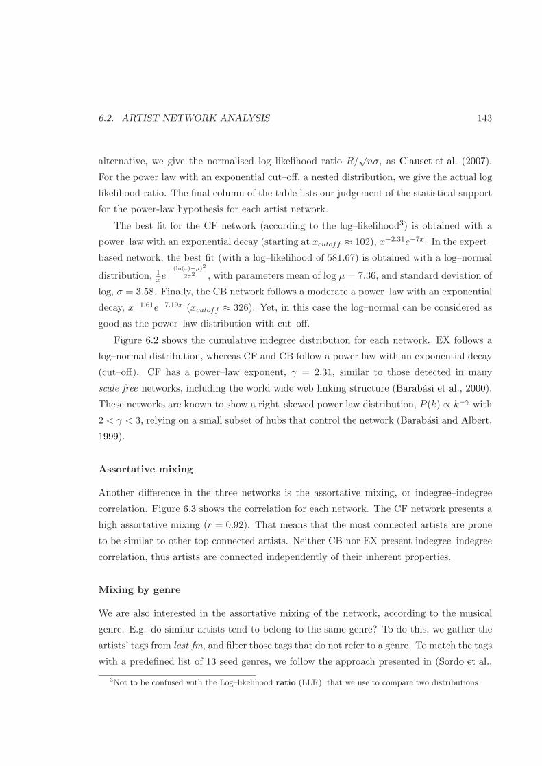
6.2. ARTIST NETWORK ANALYSIS 143
alternative, we give the normalised log likelihood ratio R/√
nσ, as Clauset et al. (2007).
For the power law with an exponential cut–off, a nested distribution, we give the actual log
likelihood ratio. The final column of the table lists our judgement of the statistical support
for the power-law hypothesis for each artist network.
The best fit for the CF network (according to the log–likelihood3) is obtained with a
power–law with an exponential decay (starting at xcutoff ≈ 102), x−2.31e−7x. In the expert–
based network, the best fit (with a log–likelihood of 581.67) is obtained with a log–normal
distribution, 1xe−
(ln(x)−µ)2
2σ2 , with parameters mean of log µ = 7.36, and standard deviation of
log, σ = 3.58. Finally, the CB network follows a moderate a power–law with an exponential
decay, x−1.61e−7.19x (xcutoff ≈ 326). Yet, in this case the log–normal can be considered as
good as the power–law distribution with cut–off.
Figure 6.2 shows the cumulative indegree distribution for each network. EX follows a
log–normal distribution, whereas CF and CB follow a power law with an exponential decay
(cut–off). CF has a power–law exponent, γ = 2.31, similar to those detected in many
scale free networks, including the world wide web linking structure (Barabasi et al., 2000).
These networks are known to show a right–skewed power law distribution, P (k) ∝ k−γ with
2 < γ < 3, relying on a small subset of hubs that control the network (Barabasi and Albert,
1999).
Assortative mixing
Another difference in the three networks is the assortative mixing, or indegree–indegree
correlation. Figure 6.3 shows the correlation for each network. The CF network presents a
high assortative mixing (r = 0.92). That means that the most connected artists are prone
to be similar to other top connected artists. Neither CB nor EX present indegree–indegree
correlation, thus artists are connected independently of their inherent properties.
Mixing by genre
We are also interested in the assortative mixing of the network, according to the musical
genre. E.g. do similar artists tend to belong to the same genre? To do this, we gather the
artists’ tags from last.fm, and filter those tags that do not refer to a genre. To match the tags
with a predefined list of 13 seed genres, we follow the approach presented in (Sordo et al.,
3Not to be confused with the Log–likelihood ratio (LLR), that we use to compare two distributions
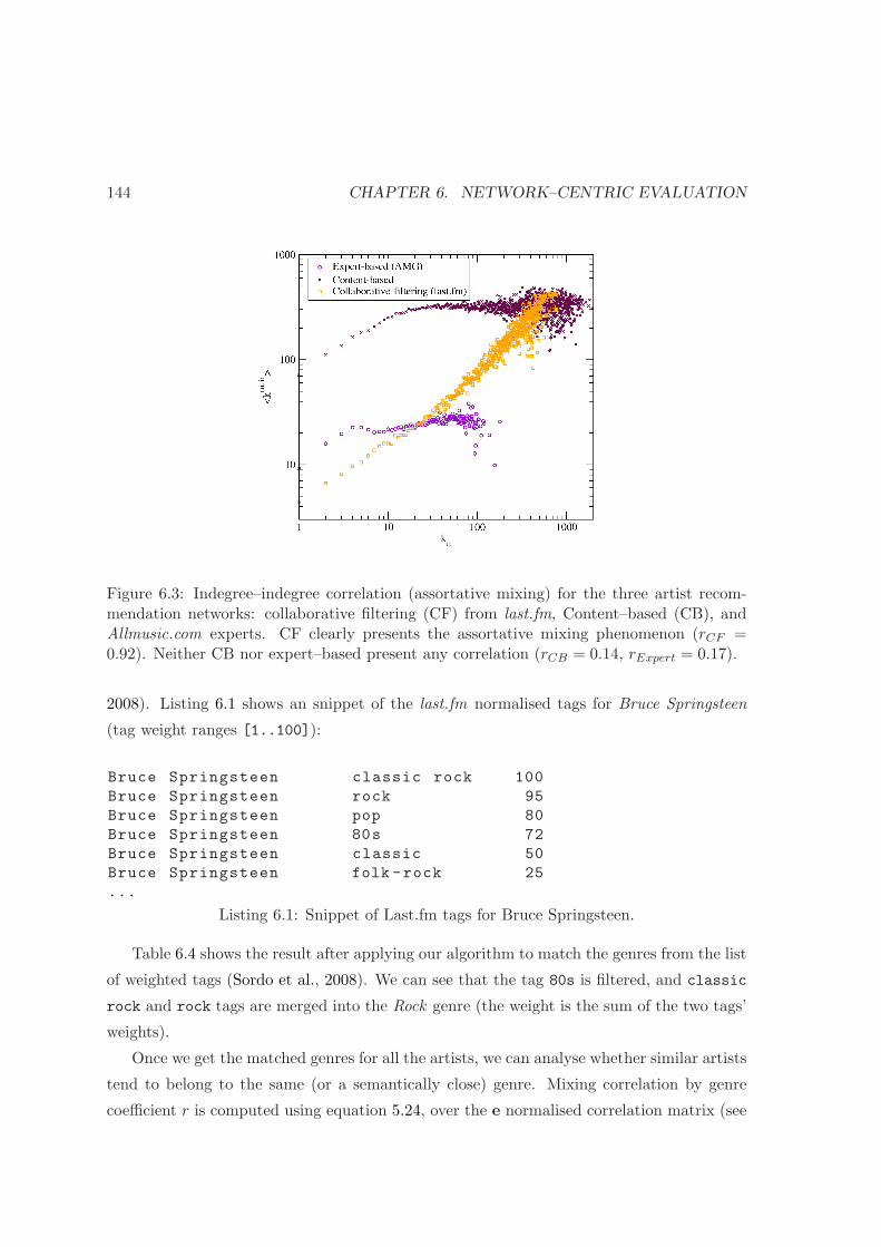
144 CHAPTER 6. NETWORK–CENTRIC EVALUATION
Figure 6.3: Indegree–indegree correlation (assortative mixing) for the three artist recom-mendation networks: collaborative filtering (CF) from last.fm, Content–based (CB), andAllmusic.com experts. CF clearly presents the assortative mixing phenomenon (rCF =0.92). Neither CB nor expert–based present any correlation (rCB = 0.14, rExpert = 0.17).
2008). Listing 6.1 shows an snippet of the last.fm normalised tags for Bruce Springsteen
(tag weight ranges [1..100]):
Bruce Springsteen classic rock 100
Bruce Springsteen rock 95
Bruce Springsteen pop 80
Bruce Springsteen 80s 72
Bruce Springsteen classic 50
Bruce Springsteen folk -rock 25
...
Listing 6.1: Snippet of Last.fm tags for Bruce Springsteen.
Table 6.4 shows the result after applying our algorithm to match the genres from the list
of weighted tags (Sordo et al., 2008). We can see that the tag 80s is filtered, and classic
rock and rock tags are merged into the Rock genre (the weight is the sum of the two tags’
weights).
Once we get the matched genres for all the artists, we can analyse whether similar artists
tend to belong to the same (or a semantically close) genre. Mixing correlation by genre
coefficient r is computed using equation 5.24, over the e normalised correlation matrix (see
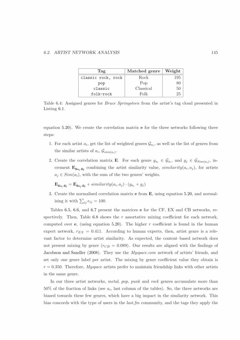
6.2. ARTIST NETWORK ANALYSIS 145
Tag Matched genre Weight
classic rock, rock Rock 195pop Pop 80
classic Classical 50folk-rock Folk 25
Table 6.4: Assigned genres for Bruce Springsteen from the artist’s tag cloud presented inListing 6.1.
equation 5.20). We create the correlation matrix e for the three networks following three
steps:
1. For each artist ai, get the list of weighted genres Gai, as well as the list of genres from
the similar artists of ai, Gsim(ai).
2. Create the correlation matrix E. For each genre gai∈ Gai
, and gj ∈ GSim(ai), in-
crement Egai,gj
combining the artist similarity value, similarity(ai, aj), for artists
aj ∈ Sim(ai), with the sum of the two genres’ weights.
Egai,gj
= Egai,gj
+ similarity(ai, aj) · (gai+ gj)
3. Create the normalised correlation matrix e from E, using equation 5.20, and normal-
ising it with∑
ij eij = 100.
Tables 6.5, 6.6, and 6.7 present the matrices e for the CF, EX and CB networks, re-
spectively. Then, Table 6.8 shows the r assortative mixing coefficient for each network,
computed over e, (using equation 5.20). The higher r coefficient is found in the human
expert network, rEX = 0.411. According to human experts, then, artist genre is a rele-
vant factor to determine artist similarity. As expected, the content–based network does
not present mixing by genre (rCB = 0.089). Our results are aligned with the findings of
Jacobson and Sandler (2008). They use the Myspace.com network of artists’ friends, and
set only one genre label per artist. The mixing by genre coefficient value they obtain is
r = 0.350. Therefore, Myspace artists prefer to maintain friendship links with other artists
in the same genre.
In our three artist networks, metal, pop, punk and rock genres accumulate more than
50% of the fraction of links (see ai, last column of the tables). So, the three networks are
biased towards these few genres, which have a big impact in the similarity network. This
bias concords with the type of users in the last.fm community, and the tags they apply the
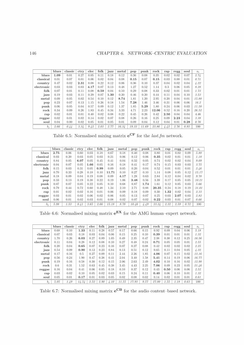
146 CHAPTER 6. NETWORK–CENTRIC EVALUATION
blues classic ctry elec folk jazz metal pop punk rock rap regg soul ai
blues 1.09 0.01 0.27 0.05 0.11 0.18 0.12 0.36 0.08 0.35 0.02 0.02 0.07 2.74classical 0.01 0.07 0.01 0.06 0.02 0.04 0.08 0.15 0.07 0.15 0.03 0.00 0.01 0.71country 0.47 0.02 2.31 0.08 0.22 0.12 0.06 0.36 0.10 0.37 0.04 0.02 0.04 4.22
electronic 0.03 0.03 0.03 4.17 0.07 0.13 0.48 1.27 0.52 1.14 0.3 0.06 0.05 8.28folk 0.07 0.01 0.11 0.08 0.59 0.04 0.10 0.29 0.08 0.33 0.02 0.01 0.01 1.73jazz 0.19 0.03 0.11 0.29 0.07 1.30 0.20 0.46 0.20 0.44 0.11 0.04 0.10 3.53
metal 0.09 0.05 0.02 0.54 0.10 0.12 8.74 1.81 1.20 2.95 0.20 0.04 0.01 15.88pop 0.23 0.07 0.13 1.15 0.26 0.18 1.54 7.28 1.46 3.46 0.31 0.06 0.06 16.2
punk 0.06 0.05 0.04 0.57 0.09 0.12 1.37 1.85 5.29 1.80 0.24 0.06 0.03 11.58rock 0.34 0.09 0.26 1.83 0.45 0.34 3.33 4.71 2.23 12.06 0.52 0.16 0.20 26.52rap 0.02 0.01 0.01 0.40 0.02 0.08 0.22 0.45 0.26 0.42 2.50 0.04 0.04 4.46
reggae 0.02 0.01 0.02 0.14 0.02 0.07 0.08 0.26 0.16 0.25 0.09 2.23 0.04 3.38soul 0.04 0.00 0.02 0.05 0.01 0.05 0.01 0.09 0.04 0.12 0.04 0.01 0.28 0.76
bj 2.66 0.44 3.34 9.42 2.03 2.77 16.34 19.33 11.69 23.86 4.42 2.76 0.93 100
Table 6.5: Normalised mixing matrix eCF for the last.fm network.
blues classic ctry elec folk jazz metal pop punk rock rap regg soul ai
blues 2.75 0.06 0.60 0.03 0.18 0.67 0.18 0.40 0.08 0.80 0.01 0.02 0.09 5.88classical 0.03 0.20 0.03 0.05 0.03 0.21 0.06 0.12 0.06 0.35 0.02 0.01 0.01 1.18country 0.84 0.05 6.07 0.05 0.45 0.41 0.04 0.32 0.05 0.74 0.02 0.02 0.04 9.09
electronic 0.04 0.07 0.05 1.66 0.05 0.16 0.18 0.41 0.17 0.74 0.15 0.03 0.03 3.75folk 0.15 0.03 0.31 0.05 0.99 0.09 0.05 0.20 0.04 0.52 0.01 0.01 0.01 2.46jazz 0.70 0.33 0.28 0.18 0.10 11.71 0.10 0.27 0.10 1.14 0.08 0.05 0.12 15.17
metal 0.18 0.09 0.04 0.19 0.08 0.09 4.17 1.28 0.63 2.84 0.12 0.04 0.02 9.78pop 0.33 0.13 0.19 0.38 0.22 0.19 1.06 3.48 0.56 3.39 0.17 0.05 0.05 10.21
punk 0.07 0.07 0.05 0.22 0.05 0.10 0.68 0.87 1.74 1.61 0.12 0.05 0.03 5.66rock 0.79 0.44 0.72 0.60 0.48 1.34 2.10 2.71 0.88 20.35 0.24 0.18 0.19 31.01rap 0.01 0.02 0.02 0.16 0.01 0.06 0.09 0.18 0.09 0.30 1.32 0.02 0.04 2.33
reggae 0.03 0.01 0.02 0.06 0.02 0.06 0.05 0.13 0.07 0.25 0.03 2.07 0.03 2.82soul 0.06 0.01 0.02 0.03 0.01 0.08 0.02 0.07 0.02 0.22 0.03 0.01 0.07 0.66
bj 5.98 1.53 8.41 3.65 2.66 15.18 8.78 10.46 4.49 33.24 2.32 2.59 0.72 100
Table 6.6: Normalised mixing matrix eEX for the AMG human–expert network.
blues classic ctry elec folk jazz metal pop punk rock rap regg soul ai
blues 0.68 0.10 1.33 0.11 0.28 0.57 0.17 0.66 0.15 0.92 0.09 0.04 0.06 5.18classical 0.07 0.03 0.18 0.03 0.04 0.06 0.15 0.25 0.10 0.39 0.01 0.01 0.01 1.32country 1.70 0.26 6.03 0.27 0.89 1.05 0.49 2.35 0.47 2.38 0.30 0.12 0.25 16.56
electronic 0.11 0.04 0.28 0.12 0.08 0.10 0.27 0.48 0.24 0.71 0.05 0.05 0.01 2.55folk 0.20 0.04 0.65 0.07 0.23 0.16 0.07 0.27 0.08 0.42 0.02 0.02 0.02 2.25jazz 0.54 0.09 0.90 0.12 0.23 0.84 0.13 0.51 0.12 0.65 0.11 0.04 0.05 4.32
metal 0.17 0.16 0.5 0.27 0.09 0.11 2.44 2.26 1.85 4.06 0.07 0.15 0.02 12.16pop 0.56 0.24 1.90 0.47 0.38 0.41 2.04 3.40 1.58 5.41 0.14 0.19 0.06 16.77
punk 0.19 0.16 0.58 0.30 0.12 0.15 2.06 2.63 2.49 4.02 0.10 0.16 0.02 12.98rock 0.6 0.31 1.52 0.63 0.45 0.38 3.45 4.43 2.25 7.06 0.09 0.23 0.05 21.46
reggae 0.16 0.04 0.41 0.06 0.05 0.18 0.10 0.37 0.12 0.43 0.50 0.06 0.06 2.52rap 0.03 0.02 0.10 0.05 0.02 0.03 0.15 0.24 0.11 0.40 0.06 0.10 0.01 1.32soul 0.05 0.01 0.17 0.01 0.03 0.05 0.02 0.08 0.02 0.14 0.02 0.01 0.01 0.61
bj 5.05 1.49 14.54 2.52 2.90 4.10 11.55 17.93 9.57 27.00 1.55 1.18 0.63 100
Table 6.7: Normalised mixing matrix eCB for the audio content–based network.

6.2. ARTIST NETWORK ANALYSIS 147
Network Mixing coeff. r
CF 0.343
EX 0.411
CB 0.089
Table 6.8: Assortative mixing by genre coefficient r for the three networks.
most. The EX and CB networks have more country artists than the CF network artists.
Also, in the expert network there is a lot of jazz artists. Additionally, in the three networks
there is an underrepresentation of the classical, folk and soul artists. The reality is that a
recommender system has to deal with biased collections, and make the best out of it.
In terms of genre cohesion, classical is always “misclassified” as pop/rock. In our case,
the problem with the classical genre is that some non–classical music artists are tagged
as classic. Our algorithm matches this tag with the seed genre Classical (see the Bruce
Springsteen example in Table 6.4). Actually, if we remove the classical genre from the list
of 13 genres, the r correlation coefficient increases by 0.1, in the CF and EX networks.
In the audio CB network, country and rock genres dominate over the rest. Country
subsumes blues, jazz and soul genres. For instance, folk artists share a high fraction of links
with country artists (eCBfolk,country = 0.65, compared with eCB
folk,folk = 0.23), yet eCBfolk,rock
also presents a high correlation. This finding is aligned with our previous research presented
in (Sordo et al., 2008), where we conclude that folk and country genres are similar, using
content–based audio similarity. Similarly, the same phenomenon happens for eCBblues,country,
and eCBjazz,country, although in the latter case it is more arguably the similarity between the
two genres.
Actually, in the CB network the bias towards rock and country genres is more prominent
than in the two other networks. Artist similarity is derived from audio track similarity, thus
preponderant genres have more chances to have links from other artists’ genres. This is the
reason why artists from infrequent genres correlate and “collapse” with the most prevalent
ones (see Table 6.7).
Contrastingly, in the experts’ network, country, jazz and soul artists present a high
intra–correlation value (a high fraction of vertices linking artists of the same genre, eEXi,i ).
For instance, eEXjazz,jazz = 11.71, and the sum of the row (last column), aEX
jazz, is 15.17. So,
given a jazz artist, 77% of his similar artists are also jazz musicians (eEXjazz,jazz
aEXjazz
= 0.77).
Similar values are found for country and soul artists. Neither in CF nor in CB networks we

148 CHAPTER 6. NETWORK–CENTRIC EVALUATION
can find these high intra–correlation values (only for the reggae genre in the CF network,
with aereggae,reggae
CF
aCFreggae
= 0.66 value).
At this point, we conclude the analysis of the similar artists’ networks. Now, the follow-
ing section presents the main findings about the correlation between artist popularity and
their prominence in the similarity network.
6.2.3 Popularity analysis
We have outlined in the previous section the main topological differences among the three
networks. We add now the popularity factor (measured with the total playcounts per artist),
by combining artists’ rank in the Long Tail with the results from the network analysis.
Two experiments are performed. The former reports the relationships among popular and
unknown artists. The latter experiment aims at analysing the correlation between artists’
indegree in the network and their popularity.
Artist similarity
Figure 6.4 depicts the correlation among an artist’s total playcounts and the total playcounts
of its similar artists. That is, given the total playcounts of an artist (x axis) it shows, in the
vertical axis, the average playcounts of its similar artists. CF network has a clear correlation
(rCF = 0.503); the higher the playcounts of a given artist, the higher the avg. playcounts of
its similar artists. The AMG human expert network presents a moderate correlation (rEX =
0.259). Thus, in some cases artists are linked according to their popularity. CB network
does not present correlation (rCB = 0.08). In this case, artists are linked independently of
their popularity.
Table 6.9 presents artist similarity divided into the three sections of the Long Tail curve.
Given an artist, ai, it shows (in %) the Long Tail location of its similar artists (results are
averaged over all artists). In the CF network, given a very popular artist, the probability
of reaching (in one click) a similar artist in the tail is zero. Actually, half of the similar
artists are located in the head part—that contains only 82 artists—, and the rest are in the
mid area. Artists in the mid part are tightly related (71.75%), and only 1/5 of the similar
artists are in the tail part. Finally, given an artist in the tail, its similar artists remain in
the same area. Contrastingly, the CB and EX networks promote the mid and tail parts
much more in all the cases (specially in the head part).

6.2. ARTIST NETWORK ANALYSIS 149
Figure 6.4: A log–log plot depicting the correlation between an artist’s total playcountsand similar artists’ playcounts (average values are shown in black, whilst grey dots displayall the values). Pearson correlation coefficient r values are: rCF = 0.503, rEX = 0.259 andrCB = 0.081.
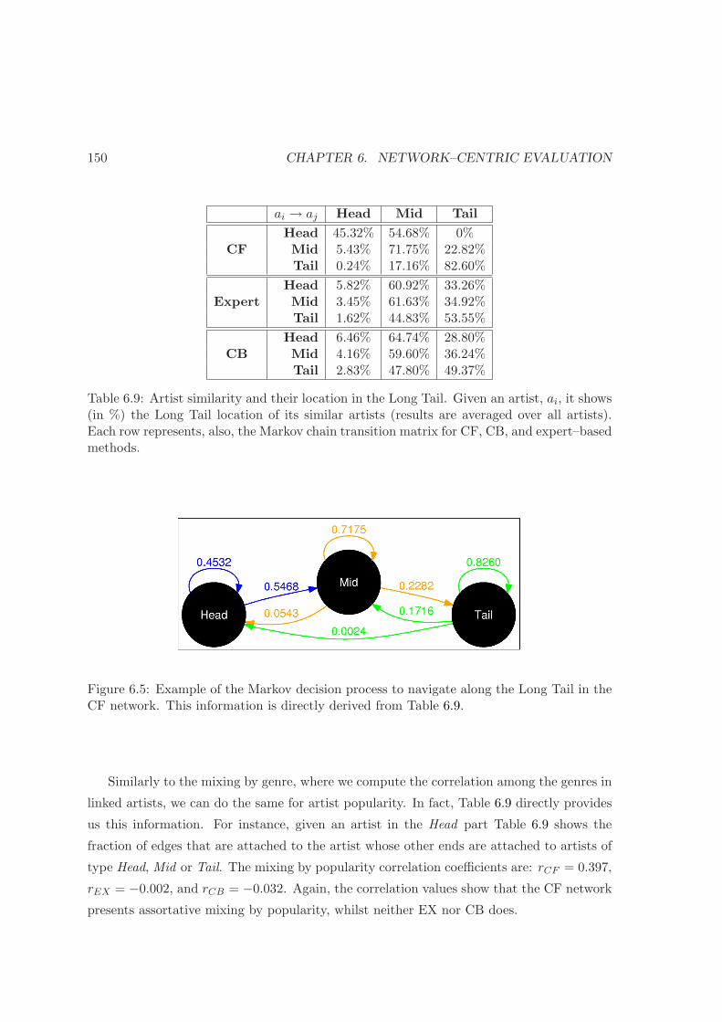
150 CHAPTER 6. NETWORK–CENTRIC EVALUATION
ai → aj Head Mid Tail
CFHead 45.32% 54.68% 0%Mid 5.43% 71.75% 22.82%Tail 0.24% 17.16% 82.60%
ExpertHead 5.82% 60.92% 33.26%Mid 3.45% 61.63% 34.92%Tail 1.62% 44.83% 53.55%
CBHead 6.46% 64.74% 28.80%Mid 4.16% 59.60% 36.24%Tail 2.83% 47.80% 49.37%
Table 6.9: Artist similarity and their location in the Long Tail. Given an artist, ai, it shows(in %) the Long Tail location of its similar artists (results are averaged over all artists).Each row represents, also, the Markov chain transition matrix for CF, CB, and expert–basedmethods.
Figure 6.5: Example of the Markov decision process to navigate along the Long Tail in theCF network. This information is directly derived from Table 6.9.
Similarly to the mixing by genre, where we compute the correlation among the genres in
linked artists, we can do the same for artist popularity. In fact, Table 6.9 directly provides
us this information. For instance, given an artist in the Head part Table 6.9 shows the
fraction of edges that are attached to the artist whose other ends are attached to artists of
type Head, Mid or Tail. The mixing by popularity correlation coefficients are: rCF = 0.397,
rEX = −0.002, and rCB = −0.032. Again, the correlation values show that the CF network
presents assortative mixing by popularity, whilst neither EX nor CB does.

6.2. ARTIST NETWORK ANALYSIS 151
k P(k), with P (0) = (1H , 0M , 0T ) π n
CF 5 (0.075H , 0.512M , 0.413T ) (0.044H , 0.414M , 0.542T ) 26
Expert 2 (0.030H , 0.560M , 0.410T ) (0.027H , 0.544M , 0.429T ) 8
CB 2 (0.038H , 0.562M , 0.400T ) (0.037H , 0.550M , 0.413T ) 7
Table 6.10: Navigation along the Long Tail of artists in terms of a Markovian stochasticprocess. Second and third columns depict the number of clicks (k) to reach the tail from thehead part, with a probability phead,tail ≥ 0.4. Fourth and fifth columns show the stationarydistribution π, as well as the number of steps, n, to reach π (with an error ≤ 10−6).
From head to tail
To simulate a user surfing the recommendation network, we apply a Markovian stochastic
process (Meyn and Tweedie, 1993). Indeed, each row in Table 6.9 can be seen as a Markov
chain transition matrix, M , where the head, mid and tail parts are the different states. For
example, Figure 6.5 shows the Markov chain for the CF network. The values of matrix M
denote the transition probabilities, pi,j , between two states i, and j (e.g. pCFhead,mid = 0.5468).
The Markovian transition matrix, Mk, denotes the probability of going from any state to
another state in k steps (clicks). The initial distribution vector, P (0), sets the probabilities
of being at a determined state at the beginning of the process. Then, P (k) = P (0) × Mk,
denotes the probability distribution after k clicks, starting in the state defined by P (0).
Using P (k) and defining P (0) = (1H , 0M , 0T ), we can get the probability of reaching any
state, starting in the head part. Table 6.10 shows the number of clicks needed to reach the
tail from the head, with a probability phead,tail ≥ 0.4. In CF, one needs five clicks to reach
the tail, whereas in CB and expert–based only two clicks are needed.
Finally, the stationary distribution π is a fixed point (row) vector whose entries sum to
1, and that satisfies π = πM . The last two columns in Table 6.10 present the stationary
distribution vector for each algorithm, and the number of steps to converge to π, with an
error ≤ 10−6. CF transition matrix needs more than three times the number of steps of
CB or EX to reach the steady state, due to the transition pCFhead,tail = 0. Furthermore, even
though the probability to stay in the tail in CF is higher than in CB or EX, this is due to
the high probability to remain in the tail once it is reached (pCFtail,tail = 0.8260).

152 CHAPTER 6. NETWORK–CENTRIC EVALUATION
CF
kin Artist Long Tail rank
976 Donald Byrd 6,362791 Little Milton 19,190772 Rufus Thomas 14,007755 Mccoy Tyner 7,700755 Joe Henderson 8,769744 R.E.M. 88738 Wayne Shorter 4,576717 U2 35712 Horace Silver 5,751709 Freddie Hubbard 7,579
Expert
kin Artist Long Tail rank
180 R.E.M. 88157 Radiohead 2137 The Beatles 1119 David Bowie 62117 Nirvana 19111 Tool 17111 Pavement 245109 Foo Fighters 45104 Soundgarden 385103 Weezer 51
CB
kin Artist Long Tail rank
1,955 George Strait 2,6321,820 Neil Diamond 1,9741,771 Chris Ledoux 13,8031,646 The Carpenters 1,6241,547 Cat Stevens 6231,514 Peter Frampton 4,4111,504 Steely Dan 1,0731,495 Lynyrd Skynyrd 6681,461 Toby Keith 2,1531,451 Charlie Daniels Band 22,201
Table 6.11: Top–10 artists with higher indegree (kin) for each recommendation network.The table shows too, the artist ranking in the Long Tail.

6.2. ARTIST NETWORK ANALYSIS 153
Artist indegree
Up to now, we have analysed the popularity in terms of the relationships among the artists.
Now, we analyse the correlation between the artists’ indegree in the network and their
popularity. As a starting point, we present in Table 6.11 the top–10 artists with the highest
indegrees for each network. CF and expert–based contains two and eight mainstream artists,
respectively. CF contains U2 and R.E.M., but the rest of the list contains more or less well
known jazz musicians, including some in the top of the tail area. The whole list for the
expert–based AMG network is made up of very popular artists. Our guess is that the
editors connect long tail artists with the most popular ones, because these popular artists
are considered influential and many bands are considered followers of these mainstream
artists. The CB network has a more eclectic top–10 list, as one would expect. Oddly enough,
there is no new or actual artists, but some classic bands and artists ranging several musical
genres.Some bands are, in fact, quite representative of a genre (e.g. Lynyrd Skynyrd, and
The Charlie Daniels Band for Southern–rock, The Carpenters for Pop in the 70’s, George
Strait for Country, and Cat Stevens for Folk/Rock). Probably, their high indegree is due
to being very influential in their respective musical styles. In some sense, there are other
bands that “cite” or imitate their sound.
Although, the results could be somewhat biased; our sampled CF and expert networks
are subsets of the whole last.fm and AMG similar artist networks, thus our sampling could
not be a good representation of the whole dataset. Furthermore, the differences in the
maximum indegree value (kin for top–1 artist) among the three networks are due to the
different sizes (N) and average degree 〈k〉 of the networks (5.47EX versus 14.13CF , and
19.80CB), but also due to the topology of the networks. CF and CB follow a power–law
cumulative indegree distribution, whereas EX best fits a log–normal distribution. Therefore
the maximum indegree kin for EX is much smaller than that of CF or CB.
To conclude this analysis, Figure 6.6 shows the correlation between artists’ indegree
(kin), and artists’ popularity, using artist’s total playcounts. The figure shows whether
the artists with higher indegree in the network (hubs) are the most popular artists. Again
we can see that in CF and expert–based networks, the artists with higher indegree (hubs)
are mostly located in the head and mid part, whereas in CB they are more spread out
through all the curve. Both CF and expert–based networks confirm the expectations, as
there is a clear correlation between the artist indegree and total playcounts (rCF = 0.621,
and rEX = 0.475). Artists with high indegree are the most popular ones. In CB, given

154 CHAPTER 6. NETWORK–CENTRIC EVALUATION
Figure 6.6: A log–log plot showing the correlation between artist indegree (kin, in horizontalaxis) and its total playcounts (avg. values in black), in vertical axis. Pearson r values are:rCF = 0.621, rEX = 0.475, and rCB = 0.032.

6.2. ARTIST NETWORK ANALYSIS 155
a high indegree value it contains, on average, artists ranging different levels of popularity
(rCB = 0.032).
6.2.4 Discussion
The results show that the last.fm social–based recommender tends to reinforce popular
artists, at the expense of discarding less–known music. Thus, the popularity effect derived
from the community of users has consequences in the recommendation network. This reveals
a somewhat poor discovery ratio when just browsing through the network of similar music
artists. It is not easy to reach relevant long tail artists, starting from the head or mid
parts (see Table 6.10). This could be related to the existence of positive feedback loops
in social–based recommenders. The first users that enters to the system heavily affects
the initial relationships among the items. After that, the users that come later, find an
environment shaped by earlier users. These new users will be affected by the early raters that
create the similarities among the items. Thus, positive feedback also affects the navigation
through the Long Tail. Given a long tail artist, its similar artists are all located in the tail
area as well. This does not always guarantee novel music recommendations; a user that
knows an artist in the Long Tail quite well is likely to know most of the similar artists
too (e.g. the solo project of the band’s singer, collaborations with other musicians, and
so on). Thus, these might not be considered good novel recommendations to that user,
but familiar ones. CF contains, then, all the elements to conclude that popularity has a
strong effect in the recommendations, because: (i) it presents assortative mixing (indegree–
indegree correlation), see Figure 6.3, (ii) there is a strong correlation between an artist’s
total playcounts and the total playcounts of its similar artists (see Figure 6.4), (iii) most of
the hubs in the network are popular artists (see Figure 6.6), and (iv) it is not easy to reach
relevant Long Tail artists, starting from the head or mid parts (see Table 6.10).
Human expert–based recommendations are more expensive to create and have a smaller
Long Tail coverage compared to automatically generated recommendations like those in
CF and CB. Regarding popularity, the hubs in the expert network are comprised of main-
stream music, thus potentially creating a network dominated by popular artists (see Table
6.11 and Figure 6.6). However, the topology —specially the log–normal cumulative indegree
distribution— indicates that these artists do not act as hubs, as in the power law distribu-
tions with a γ exponent between 2 and 3 (Barabasi and Albert, 1999). Furthermore, the
expert network does not present assortative mixing (see Figure 6.3), so artists are linked in

156 CHAPTER 6. NETWORK–CENTRIC EVALUATION
a heterogeneous way; popular artists are connected with other less–known artists and the
other way around (see Table 6.9 and Figure 6.4).
According to the stationary distribution π (see Table 6.10), the key Long Tail area in the
CB and EX networks are the artists in the mid part. These artists allow users to navigate
inside the Long Tail acting as entry points, as well as main destinations when leaving the
Long Tail. Also, users that listen to mainly very Long Tail music are likely to discover
unknown artists —for them— that are in the mid part, and that are easily reachable from
the artists in the tail. One should pay attention to the quality data in the Long Tail as well.
Assuming that there exists some extremely poor quality music, CB is not able to clearly
discriminate against it. In some sense, the popularity effect drastically filters all these low
quality items. Although, it has been proved by Salganik et al. (2006) that increasing the
strength of social influence increased both inequality and unpredictability of success and,
as a consequence, popularity was only partly determined by quality.
6.3 User network analysis
One of the main goals of neighbourhood–based recommendation algorithms is to find like–
minded people, and through them, discover unknown music. In this sense, a user similarity
network resembles a social network, automatically connecting people that share similar
interests.
We present an evaluation of two user similarity networks. Both networks are derived
from the users’ listening habits. The first one is based on collaborative filtering (CF). Again,
we gather this information from last.fm. For the second network we use content–based audio
similarity (CB) to compute user similarity.
6.3.1 Datasets
Social–based, collaborative filtering network
User similarity is gathered from last.fm., using Audioscrobbler webservices. For each user
we collect the top–20 similar users. Last.fm derives user similarity from the item–based
approach, so it connects users that share common musical tastes. Table 6.12 shows the
number of users and links in the network.
6.3. USER NETWORK ANALYSIS 157
Number of users Number of relations
Last.fm social filtering (CF) 158,209 3,164,180
Content–based (CB) 207,863 4,137,500
Table 6.12: Datasets for the user similarity networks.
Content–based network
User similarity for the CB network is computed using content–based audio analysis from a
music collection (T ) of 1.3 Million tracks of 30 sec. samples. To compute similar users we
used all the tracks, Tu, that a user u has listened to. For each track, ti ∈ Tu, we obtain the
most similar tracks like this:
sim(ti) = argmin∀t∈T
(distance(ti, t)), (6.3)
and get all the users, Usim(ti), that listened to any track similar to ti. The list of (top–20)
similar users of u is composed by the users in Usim(ti) for all ti ∈ Tu, weighted by the audio
similarity distance:
similar users(u) =⋃
Usim(ti),∀ti ∈ Tu (6.4)
To select the maximum number of similar users per user we compute, for all the users,
the average distance between the user and her top–20 similar users. We use this average
distance as a threshold to get the top–N most similar users, setting a maximum of N = 20.
The main difference between the two approaches is that in CF two users have to share
at least one artist in order to become —potentially— similar. In the CB we can have two
similar users that do not have share any artist, yet the music they listen to is similar. For
instance, two users that listen to, respectively, ui = [Ramones, The Clash, Buzzcocks, and
Dead Kennedys], and uj = [Sex Pistols, The Damned, The Addicts, and Social Distortion]
could be very similar using CB, but not using CF (unless the recommender system also
makes use of higher–level information, such as a tag cloud representation of the artists).
However, in the CB network if no constraint is applied to the user profiles, a user with
a high number of total playcounts has a higher chance of being considered similar to other
users.
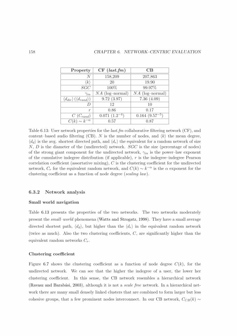
158 CHAPTER 6. NETWORK–CENTRIC EVALUATION
Property CF (last.fm) CB
N 158,209 207,863
〈k〉 20 19.90
SGC 100% 99.97%
γin NA (log–normal) NA (log–normal)
〈ddir〉 (〈drand〉) 9.72 (3.97) 7.36 (4.09)
D 12 10
r 0.86 0.17
C (Crand) 0.071 (1.2−4) 0.164 (9.57−5)
C(k) ∼ k−α 0.57 0.87
Table 6.13: User network properties for the last.fm collaborative filtering network (CF), andcontent–based audio filtering (CB). N is the number of nodes, and 〈k〉 the mean degree,〈dd〉 is the avg. shortest directed path, and 〈dr〉 the equivalent for a random network of sizeN , D is the diameter of the (undirected) network. SGC is the size (percentage of nodes)of the strong giant component for the undirected network, γin is the power–law exponentof the cumulative indegree distribution (if applicable), r is the indegree–indegree Pearsoncorrelation coefficient (assortative mixing), C is the clustering coefficient for the undirectednetwork, Cr for the equivalent random network, and C(k) ∼ k−α is the α exponent for theclustering coefficient as a function of node degree (scaling law).
6.3.2 Network analysis
Small world navigation
Table 6.13 presents the properties of the two networks. The two networks moderately
present the small–world phenomena (Watts and Strogatz, 1998). They have a small average
directed shortest path, 〈dd〉, but higher than the 〈dr〉 in the equivalent random network
(twice as much). Also the two clustering coefficients, C, are significantly higher than the
equivalent random networks Cr.
Clustering coefficient
Figure 6.7 shows the clustering coefficient as a function of node degree C(k), for the
undirected network. We can see that the higher the indegree of a user, the lower her
clustering coefficient. In this sense, the CB network resembles a hierarchical network
(Ravasz and Barabasi, 2003), although it is not a scale free network. In a hierarchical net-
work there are many small densely linked clusters that are combined to form larger but less
cohesive groups, that a few prominent nodes interconnect. In our CB network, CCB(k) ∼

6.3. USER NETWORK ANALYSIS 159
Figure 6.7: Clustering coefficient C(k) versus degree k. The CB network resembles ahierarchical network (CCB(k) ∼ k−0.87), although it is not a scale free network.
k−0.87, starting at k = 20 the α = 0.87 is close to the scaling law, C(k) ∼ k−1. The scaling
law is used to determine the presence of hierarchy in real networks (Ravasz and Barabasi,
2003).
C(k) is computed for the undirected networks. That is the reason that the CCB(k) ∼k−0.87 power law starts at k = 20. In the undirected network most of the nodes have k ≥ 20
—the node outlinks, kout, plus the incoming links they receive kin. However, in some cases
a node has kout < 20, because the threshold has been applied (see the creation of datasets,
in section 6.3.1). These few nodes are located on the left side of Figure 6.7 (0 < k < 20),
and are discarded to compute C(k).
Indegree distribution
Table 6.14 presents the model selection for the indegree distribution. For each network we
give a p–value of the fit to the power-law model (first column). A higher p–value means that
the distribution is likely to follow a power–law. We also present the likelihood ratios for
the alternative distributions (power–law with an exponential cut–off, and log–normal), and
the p–values for the significance of the likelihood ratio tests. In this case, a p–value close
to zero means that the alternative distribution can also fit the distribution (see section 4.4
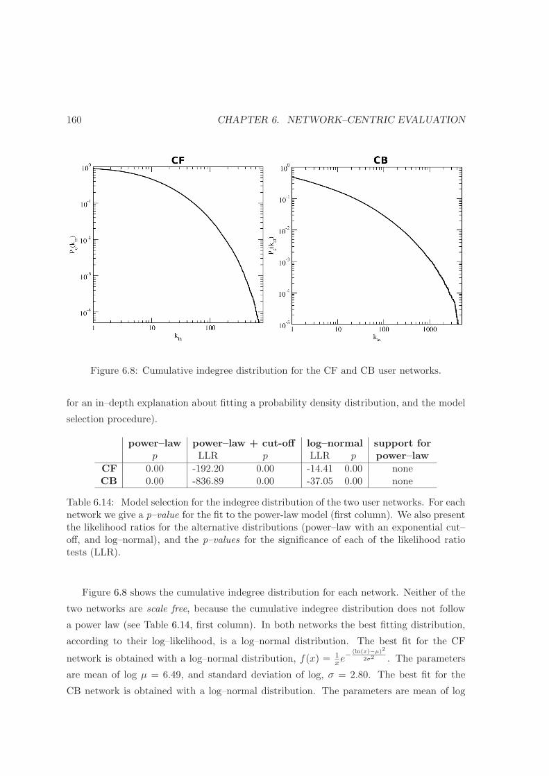
160 CHAPTER 6. NETWORK–CENTRIC EVALUATION
Figure 6.8: Cumulative indegree distribution for the CF and CB user networks.
for an in–depth explanation about fitting a probability density distribution, and the model
selection procedure).
power–law power–law + cut-off log–normal support forp LLR p LLR p power–law
CF 0.00 -192.20 0.00 -14.41 0.00 noneCB 0.00 -836.89 0.00 -37.05 0.00 none
Table 6.14: Model selection for the indegree distribution of the two user networks. For eachnetwork we give a p–value for the fit to the power-law model (first column). We also presentthe likelihood ratios for the alternative distributions (power–law with an exponential cut–off, and log–normal), and the p–values for the significance of each of the likelihood ratiotests (LLR).
Figure 6.8 shows the cumulative indegree distribution for each network. Neither of the
two networks are scale free, because the cumulative indegree distribution does not follow
a power law (see Table 6.14, first column). In both networks the best fitting distribution,
according to their log–likelihood, is a log–normal distribution. The best fit for the CF
network is obtained with a log–normal distribution, f(x) = 1xe−
(ln(x)−µ)2
2σ2 . The parameters
are mean of log µ = 6.49, and standard deviation of log, σ = 2.80. The best fit for the
CB network is obtained with a log–normal distribution. The parameters are mean of log
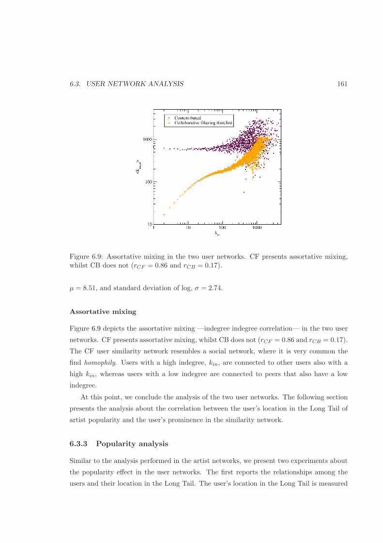
6.3. USER NETWORK ANALYSIS 161
Figure 6.9: Assortative mixing in the two user networks. CF presents assortative mixing,whilst CB does not (rCF = 0.86 and rCB = 0.17).
µ = 8.51, and standard deviation of log, σ = 2.74.
Assortative mixing
Figure 6.9 depicts the assortative mixing —indegree indegree correlation— in the two user
networks. CF presents assortative mixing, whilst CB does not (rCF = 0.86 and rCB = 0.17).
The CF user similarity network resembles a social network, where it is very common the
find homophily. Users with a high indegree, kin, are connected to other users also with a
high kin, whereas users with a low indegree are connected to peers that also have a low
indegree.
At this point, we conclude the analysis of the two user networks. The following section
presents the analysis about the correlation between the user’s location in the Long Tail of
artist popularity and the user’s prominence in the similarity network.
6.3.3 Popularity analysis
Similar to the analysis performed in the artist networks, we present two experiments about
the popularity effect in the user networks. The first reports the relationships among the
users and their location in the Long Tail. The user’s location in the Long Tail is measured
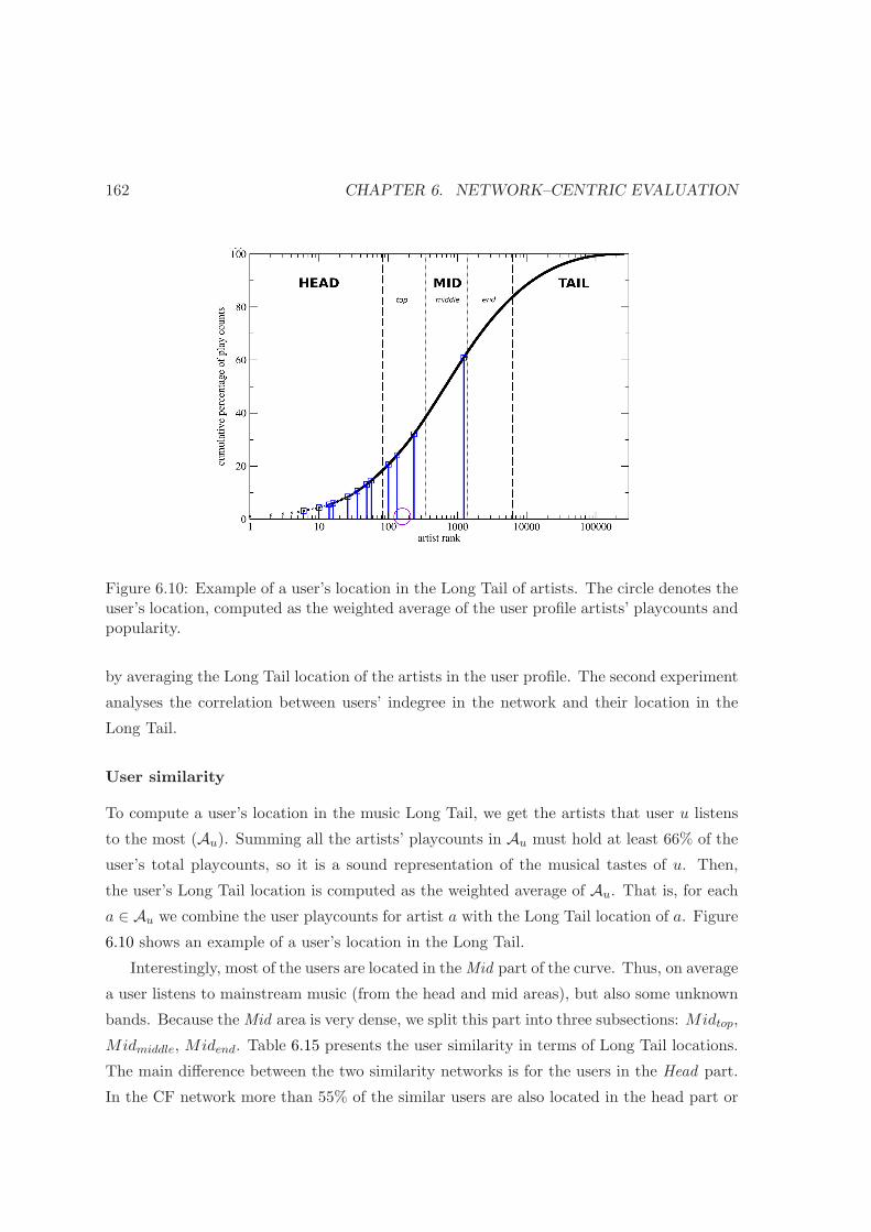
162 CHAPTER 6. NETWORK–CENTRIC EVALUATION
Figure 6.10: Example of a user’s location in the Long Tail of artists. The circle denotes theuser’s location, computed as the weighted average of the user profile artists’ playcounts andpopularity.
by averaging the Long Tail location of the artists in the user profile. The second experiment
analyses the correlation between users’ indegree in the network and their location in the
Long Tail.
User similarity
To compute a user’s location in the music Long Tail, we get the artists that user u listens
to the most (Au). Summing all the artists’ playcounts in Au must hold at least 66% of the
user’s total playcounts, so it is a sound representation of the musical tastes of u. Then,
the user’s Long Tail location is computed as the weighted average of Au. That is, for each
a ∈ Au we combine the user playcounts for artist a with the Long Tail location of a. Figure
6.10 shows an example of a user’s location in the Long Tail.
Interestingly, most of the users are located in the Mid part of the curve. Thus, on average
a user listens to mainstream music (from the head and mid areas), but also some unknown
bands. Because the Mid area is very dense, we split this part into three subsections: Midtop,
Midmiddle, Midend. Table 6.15 presents the user similarity in terms of Long Tail locations.
The main difference between the two similarity networks is for the users in the Head part.
In the CF network more than 55% of the similar users are also located in the head part or
6.3. USER NETWORK ANALYSIS 163
ui → uj Head Midtop Midmiddle Midend Tail
CFHead 9.36% 46.22% 26.66% 14.97% 2.78%Mid 1.11% 20.52% 41.96% 30.22% 6.18%Tail 0.41% 7.23% 26.98% 42.43% 22.95%
CBHead 10.64% 23.70% 34.42% 25.91% 5.32%Mid 3.79% 15.43% 37.95% 34.92% 7.90%Tail 1.92% 8.34% 26.94% 40.81% 21.98%
Table 6.15: Similarities among the users, and their location in the Long Tail. Given a user,ui, it shows (in %) the Long–Tail location of its similar artists, uj . The results are averagedover all users in each part of the curve.
P(3), with P (0) = (0, 0, 1, 0, 0) π n
CF (0.210Left, 0.407Stay, 0.383Right) (0.012Head, 0.199M−top, 0.407M−mid, 0.309M−end, 0.074Tail) 5
CB (0.190Left, 0.368Stay, 0.442Right) (0.039Head, 0.151M−top, 0.368M−mid, 0.351M−end, 0.091Tail) 5
Table 6.16: Long Tail navigation in terms of a Markovian stochastic process. Second columnshows the probability distribution of a user in the Midmiddle after 3 clicks. Third and fourthcolumns show the stationary distribution π, as well as the number of steps, n, to reach π(with an error ≤ 10−5).
in the top of the Mid part (Midtop), whilst in the CB network this value is less than 35%.
We represent each row in Table 6.15 as a Markov transition matrix. Using a Markovian
stochastic process we can simulate a user surfing the similarity network. In the artist
network (see section 6.2.2), we were interested in the navigation from head to tail artists.
Now, in the user network, the users are already located in the Long Tail according to the
artists’ popularity in their profile. Thus, we are more interested in the Long Tail location of
the similar users, rather than in the navigation from head to tail users. For instance, using
P (3) and defining P (0) = (0Head, 0M−top, 1M−mid, 0M−end, 0Tail), we get the probability of a
user located in the mid part of the curve (Midmiddle) to move to the left side (Head, and
Mtop), to stay in the same Midmiddle area, or to move to the right (Midend, and Tail). Table
6.16 shows the probability distributions. Second column shows the probability distribution
of a user located in the Midmiddle after 3 clicks, P (3). The CF network has a tendency to
stay in the same Midmiddle area, whilst in the CB network the user slightly moves towards
the right, tail, area. In both cases, the probability to move to the Head (left) is around 0.2.
Table 6.16 also shows the stationary distribution π, that satisfies π = πM . The last
two columns present the stationary distribution vector for each algorithm, and the number
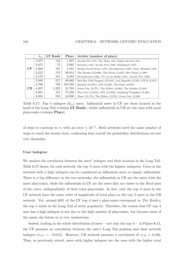
164 CHAPTER 6. NETWORK–CENTRIC EVALUATION
kin LT Rank Plays Artists (number of plays)
CF
2,877 123 1,307 Arcade Fire (47), The Shins (43), Sufjan Stevens (42)
2,675 75 2,995 Interpol (116), Arcade Fire (108), Radiohead (107)
2,266 191 4,585 Broken Social Scene (172), Decemberists (128), Arch. Helsinki (128)
2,225 176 38,614 The Beatles (23,090), The Doors (1,822), Bob Dylan (1,588)
2,173 101 3,488 Decemberists (106), TV on the Radio (101), Arcade Fire (100)
CB
5,568 217 88,689 Red Hot Chili Peppers (27,618), Led Zeppelin (6,595), GN’R (3,457)
4,706 789 105,768 Interpol (31,281), AFI (5,358), The Faint (3,056)
4,207 1,222 21,762 Green Day (8,271), The Killers (4,040), The Strokes (2,184)
3,991 121 77,433 The Cure (13,945), NIN (12,938), Smashing Pumpkins (8,460)
3,884 550 44,006 Muse (19,178), The Killers (3,255), Green Day (3,168)
Table 6.17: Top–5 indegree (kin) users. Influential users in CF are those located in thehead of the Long Tail (column LT Rank), whilst influentials in CB are the ones with mostplaycounts (column Plays).
of steps to converge to π, with an error ≤ 10−5. Both networks need the same number of
steps to reach the steady state, confirming that overall the probability distributions are not
very dissimilar.
User indegree
We analyse the correlation between the users’ indegree and their location in the Long Tail.
Table 6.17 shows, for each network, the top–5 users with the highest indegrees. Users in the
network with a high indegree can be considered as influential users or simply influentials.
There is a big difference in the two networks; the influentials in CB are the users with the
most playcounts, while the influentials in CF are the users that are closer to the Head part
of the curve, independently of their total playcounts. In fact, only the top–4 users in the
CF network have the same order of magnitude of total plays as the top–5 users in the CB
network. Yet, around 60% of the CF top–4 user’s playcounts correspond to The Beatles,
the top–1 artist in the Long Tail of artist popularity. Therefore, the reason that CF top–4
user has a high indegree is not due to the high number of playcounts, but because most of
the music she listens to is very mainstream.
Indeed, looking at the whole distribution of users —not only the top–5— in Figure 6.11,
the CF presents no correlation between the user’s Long Tail position and their network
indegree (rCF = −0.012). However, CB network presents a correlation of rCB = 0.446.
Thus, as previously stated, users with higher indegree are the ones with the higher total

6.3. USER NETWORK ANALYSIS 165
Figure 6.11: Correlation between users’ indegree and total playcounts. CB has a correlationof rCB = 0.446, whilst CF does not present any correlation (rCF = −0.012).
playcounts in the CB network.
6.3.4 Discussion
The results of the analysis shows that the CB user similarity network resembles a hierarchical
network (with the exception that CB is not a scale–free network). Thus, in the CB network
there are a few nodes that are connecting smaller clusters. These nodes are the ones
with the highest indegree which, according to Figure 6.11, are the ones with higher total
playcounts. Therefore, the users that listen to more music are the authorities in the CB
network, independently of the quality or popularity of the music they listen to. This affects
the navigation of the user similarity network. Contrastingly, in the CF network the users
with a higher indegree are the ones that listen to more mainstream music. These users could
have an impact for a recommender algorithm that uses user–based, instead of item–based,
recommendations.
The key Long Tail area in the two user similarity networks is the Mid part. This area
concentrates most of the users. To improve music discovery through user similarity, the
recommendation algorithm should also promote users in the tail area. When computing
user similarity, a recommender should take into account the users’ location in the Long Tail
curve.
An important missing aspect in our analysis is the dynamics of the user networks. It

166 CHAPTER 6. NETWORK–CENTRIC EVALUATION
would be interesting to detect who are the tastemakers (or trendsetters). Users that create
trends and have an impact in the musical tastes of other users are very relevant. This is
related with the taxonomy of users presented in section 3.2.1. Ideally, the Savants should
be correlated with the tastemakers and influentials in the network. Detecting and tracking
these users is a key point to improve music discovery through the network of similar users.
However, detecting tastemakers can only be achieved by constantly gathering information
about the users’ music consumption. This way, we could analyse the dynamics and evolution
of the user similarity network.
6.4 Summary
Recommender systems should assist us in the process of filtering and discovering relevant
information hidden in the Long Tail. Popularity is the element that defines the characteristic
shape of the Long Tail. We measure popularity in terms of total playcounts, and the Long
Tail model is used in order to rank all music artists. We have analysed the topology and
the popularity bias in two music recommendation scenarios; artist and user similarity. As
expected by its inherent social component, the collaborative filtering approach is prone to
popularity bias. This has some consequences on the discovery ratio, as well as navigation
through the Long Tail.
Music recommender systems have to deal with biased datasets; a bias towards main-
stream popular artists, towards a few prominent musical genres, or towards a particular
type of user. Assortative mixing measures the correlation of these elements in the simi-
larity network. In this sense, it is important to understand which contextual attributes
have an impact when computing artist similarity (e.g. popularity, genre, decade, language,
activity, etc.), or user similarity (e.g. age, race, language, etc.). The Last.fm social–based
recommender presents several assortative mixing patterns. The artist network has assor-
tative mixing on the nodes’ indegree, but also presents mixing by genre, and mixing by
popularity; i.e. the classical homophily issues that arise in social networks. Yet, as we
will see in the next chapter, this does not necessarily have an impact on the quality of the
recommendations.
The temporal effects in the Long Tail are another aspect one should take into account.
Some new artists can be very popular, gathering a spike of attention when they release an
album, but then they can slowly move towards the mid or tail area of the curve as time goes
6.4. SUMMARY 167
by. Thus, one–time hit items can be lost and forgotten in the Long Tail. Indeed, the music
back–catalogue located in the Long Tail is an example of old and forgotten items that offer
the possibility to be re–discovered by the users. A recommender system should be able to
present and recommend these items to the user.
Links with the following chapters
We have presented a network–centric analysis of the similarities between artists, and be-
tween users. The network–based approach does not put the user into the evaluation loop.
Without any user intervention it is impossible to evaluate the quality and user satisfac-
tion of the recommendations, which does not necessarily correlate with predicted accuracy
(McNee et al., 2006). So, we still need to evaluate the quality of the recommendations as
well as the popularity effect when providing recommendations to the users. For this reason,
we present the user–based evaluation in the next chapter.

168 CHAPTER 6. NETWORK–CENTRIC EVALUATION
Chapter 7
User–centric evaluation
Up to now, we have presented a user agnostic network–based analysis of the recommenda-
tions. In this chapter we present a user–centric evaluation of the recommender algorithms.
This user–based approach focuses on evaluating the user’s perceived quality and usefulness
of the recommendations. The evaluation method considers not only the subset of items
that the user has interacted with, but also the items outside the user’s profile. The recom-
mender algorithm predicts recommendations to a particular user —taking into account her
profile—, and then the user provides feedback about the recommended items. Figure 7.1
depicts the approach.
7.1 Music Recommendation Survey
We aim at measuring the novelty and the perceived quality of music recommendation, as
neither system– nor network–centric approaches can measure these two aspects. However,
we need to explicitly ask the users whether they already know the provided recommendations
or not.
The proposed experiment is based on providing song recommendations to users, using
three different music recommendation algorithms. Feedback gathered from the users consists
of (i) whether a user already knows the song, and (ii) the relevance of the recommendations
—whether she likes the recommended song or not.
169
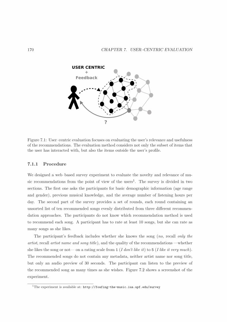
170 CHAPTER 7. USER–CENTRIC EVALUATION
Figure 7.1: User–centric evaluation focuses on evaluating the user’s relevance and usefulnessof the recommendations. The evaluation method considers not only the subset of items thatthe user has interacted with, but also the items outside the user’s profile.
7.1.1 Procedure
We designed a web–based survey experiment to evaluate the novelty and relevance of mu-
sic recommendations from the point of view of the users1. The survey is divided in two
sections. The first one asks the participants for basic demographic information (age range
and gender), previous musical knowledge, and the average number of listening hours per
day. The second part of the survey provides a set of rounds, each round containing an
unsorted list of ten recommended songs evenly distributed from three different recommen-
dation approaches. The participants do not know which recommendation method is used
to recommend each song. A participant has to rate at least 10 songs, but she can rate as
many songs as she likes.
The participant’s feedback includes whether she knows the song (no, recall only the
artist, recall artist name and song title), and the quality of the recommendations —whether
she likes the song or not— on a rating scale from 1 (I don’t like it) to 5 (I like it very much).
The recommended songs do not contain any metadata, neither artist name nor song title,
but only an audio preview of 30 seconds. The participant can listen to the preview of
the recommended song as many times as she wishes. Figure 7.2 shows a screenshot of the
experiment.
1The experiment is available at: http://foafing-the-music.iua.upf.edu/survey

7.1. MUSIC RECOMMENDATION SURVEY 171
Figure 7.2: Screenshot of the Music recommendation survey.
7.1.2 Datasets
The three music recommendation algorithms used are: collaborative filtering (CF), content–
based audio similarity (CB), and a hybrid approach (HY) combining Allmusic.com human
expert information, and content–based similarity. CF song similarity comes, again, from
last.fm2, using the Audioscrobbler web services (API v1.0). The CB method is the one
explained in section 6.2.1, equation 6.1. Hybrid method (HY) is based on combining related
artists from Allmusic.com musicologists, and CB audio similarity at track level. That is,
to get the similar tracks from a seed track, first it gets the related artists (according to the
AMG human experts) of the artist’s seed track. Then, it ranks the retrieved tracks from
the related artists using content–based audio similarity with the seed track.
7.1.3 Participants
In order to characterise the participants, at the beginning of the survey they were asked
to provide some basic demographic information (age range, and gender), as well as the
2See for example http://www.last.fm/music/U2/_/One/+similar

172 CHAPTER 7. USER–CENTRIC EVALUATION
participants musical background knowledge, the average number of listening hours per day
(more than 4 hours a day, between 2 and 4 hours a day, less than 2 hours a day, almost
never listen to music), and the context while listening to music. All the fields were optional,
so the participants could fill–in or not the information (only 9 participants did not fill–in
all the data). Regarding the musical background, the survey offered the following single
choice options:
• None: no particular interest in music related topics.
• Basic: lessons at school, reading music magazines, blogs, etc.
• Advanced: regular choir singing, amateur instrument playing, remixing or editing
music with the computer, etc.
• Professional: professional musician —conductor, composer, high level instrument
player—, music conservatory student, audio engineer, etc.
Regarding the context while listening to music, the participants were asked to choose
(multiple selection was allowed) the situations were they often listen to music. The options
are:
• While working,
• Reading,
• Cleaning,
• Traveling,
• Doing sport,
• Cooking,
• Usually I just listen to music (and don’t do anything else), and
• Other (please specify)
Furthermore, musical tastes of the participants were modelled using some seed tracks of
their top–20 most played artists from their last.fm profile. These seed tracks are the ones
used to provide song similarity using CF, CB and HY approaches.
To assemble a significant number of participants, we sent an email to the MIR–list3 that
described the survey and the procedure. Also, the survey was kindly announced in Paul
Lamere’s Duke Listens blog4 on March 3rd, 2008.
3Message sent to [email protected] on February, 28th, 20084http://blogs.sun.com/plamere/entry/evaluating_music_recommendations
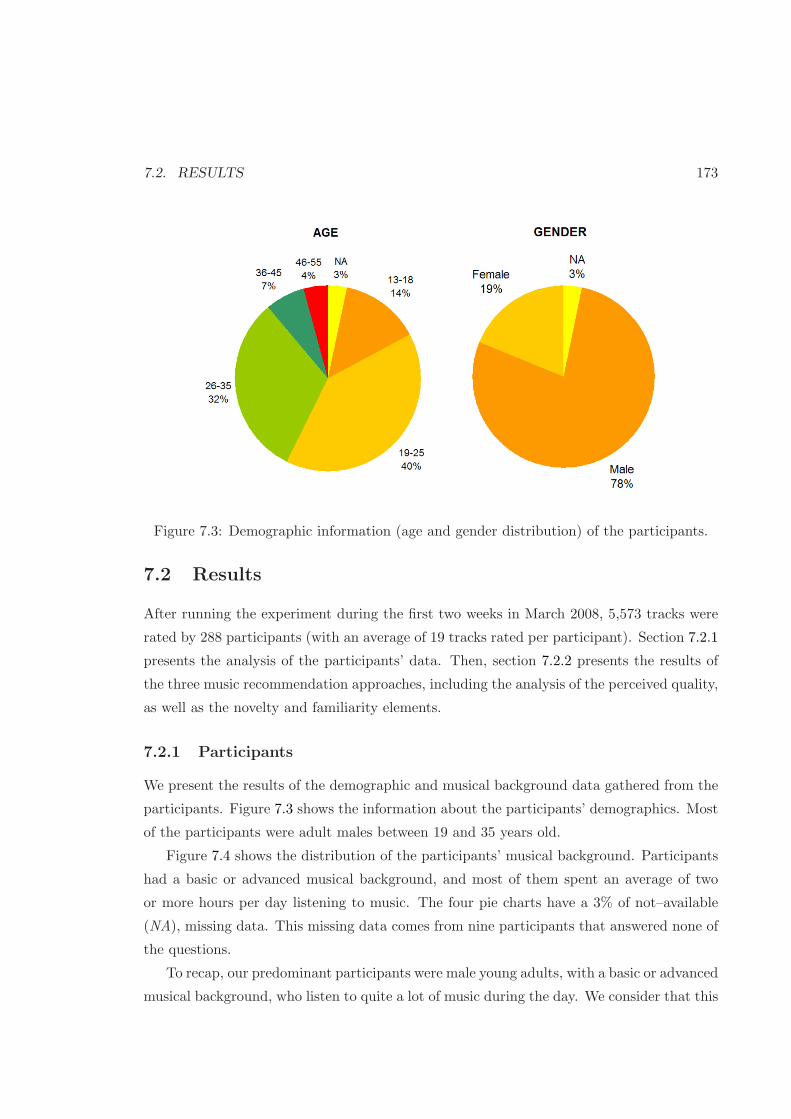
7.2. RESULTS 173
Figure 7.3: Demographic information (age and gender distribution) of the participants.
7.2 Results
After running the experiment during the first two weeks in March 2008, 5,573 tracks were
rated by 288 participants (with an average of 19 tracks rated per participant). Section 7.2.1
presents the analysis of the participants’ data. Then, section 7.2.2 presents the results of
the three music recommendation approaches, including the analysis of the perceived quality,
as well as the novelty and familiarity elements.
7.2.1 Participants
We present the results of the demographic and musical background data gathered from the
participants. Figure 7.3 shows the information about the participants’ demographics. Most
of the participants were adult males between 19 and 35 years old.
Figure 7.4 shows the distribution of the participants’ musical background. Participants
had a basic or advanced musical background, and most of them spent an average of two
or more hours per day listening to music. The four pie charts have a 3% of not–available
(NA), missing data. This missing data comes from nine participants that answered none of
the questions.
To recap, our predominant participants were male young adults, with a basic or advanced
musical background, who listen to quite a lot of music during the day. We consider that this
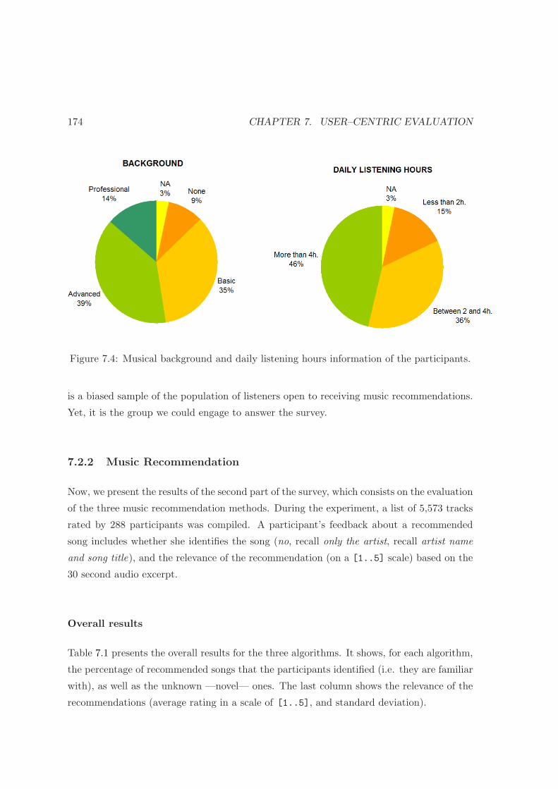
174 CHAPTER 7. USER–CENTRIC EVALUATION
Figure 7.4: Musical background and daily listening hours information of the participants.
is a biased sample of the population of listeners open to receiving music recommendations.
Yet, it is the group we could engage to answer the survey.
7.2.2 Music Recommendation
Now, we present the results of the second part of the survey, which consists on the evaluation
of the three music recommendation methods. During the experiment, a list of 5,573 tracks
rated by 288 participants was compiled. A participant’s feedback about a recommended
song includes whether she identifies the song (no, recall only the artist, recall artist name
and song title), and the relevance of the recommendation (on a [1..5] scale) based on the
30 second audio excerpt.
Overall results
Table 7.1 presents the overall results for the three algorithms. It shows, for each algorithm,
the percentage of recommended songs that the participants identified (i.e. they are familiar
with), as well as the unknown —novel— ones. The last column shows the relevance of the
recommendations (average rating in a scale of [1..5], and standard deviation).
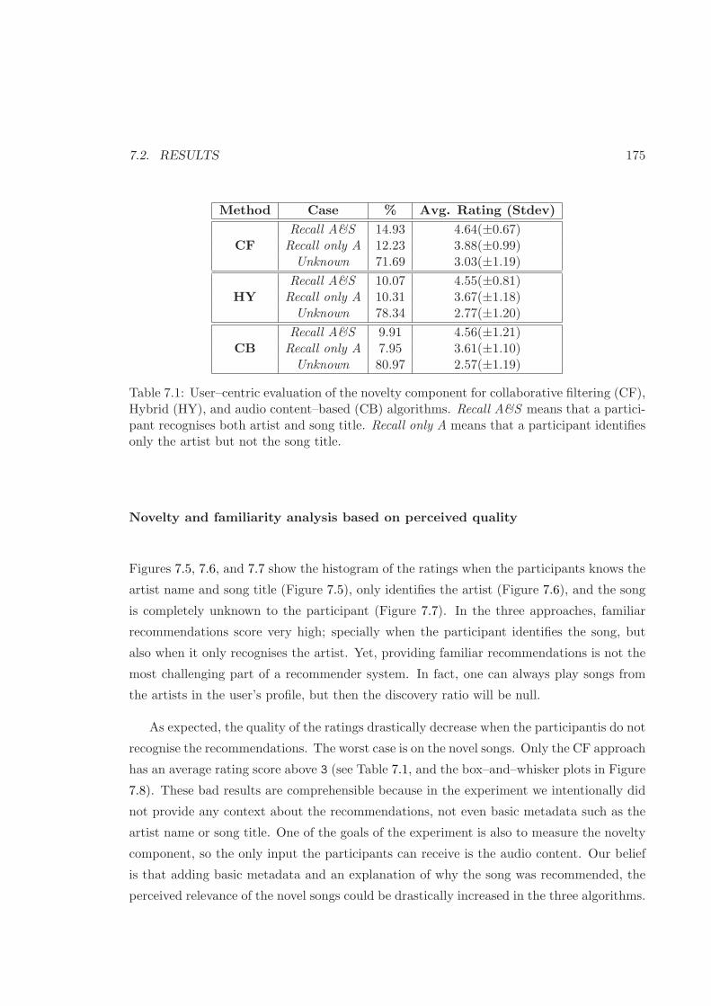
7.2. RESULTS 175
Method Case % Avg. Rating (Stdev)
CFRecall A&S 14.93 4.64(±0.67)
Recall only A 12.23 3.88(±0.99)Unknown 71.69 3.03(±1.19)
HYRecall A&S 10.07 4.55(±0.81)
Recall only A 10.31 3.67(±1.18)Unknown 78.34 2.77(±1.20)
CBRecall A&S 9.91 4.56(±1.21)
Recall only A 7.95 3.61(±1.10)Unknown 80.97 2.57(±1.19)
Table 7.1: User–centric evaluation of the novelty component for collaborative filtering (CF),Hybrid (HY), and audio content–based (CB) algorithms. Recall A&S means that a partici-pant recognises both artist and song title. Recall only A means that a participant identifiesonly the artist but not the song title.
Novelty and familiarity analysis based on perceived quality
Figures 7.5, 7.6, and 7.7 show the histogram of the ratings when the participants knows the
artist name and song title (Figure 7.5), only identifies the artist (Figure 7.6), and the song
is completely unknown to the participant (Figure 7.7). In the three approaches, familiar
recommendations score very high; specially when the participant identifies the song, but
also when it only recognises the artist. Yet, providing familiar recommendations is not the
most challenging part of a recommender system. In fact, one can always play songs from
the artists in the user’s profile, but then the discovery ratio will be null.
As expected, the quality of the ratings drastically decrease when the participantis do not
recognise the recommendations. The worst case is on the novel songs. Only the CF approach
has an average rating score above 3 (see Table 7.1, and the box–and–whisker plots in Figure
7.8). These bad results are comprehensible because in the experiment we intentionally did
not provide any context about the recommendations, not even basic metadata such as the
artist name or song title. One of the goals of the experiment is also to measure the novelty
component, so the only input the participants can receive is the audio content. Our belief
is that adding basic metadata and an explanation of why the song was recommended, the
perceived relevance of the novel songs could be drastically increased in the three algorithms.
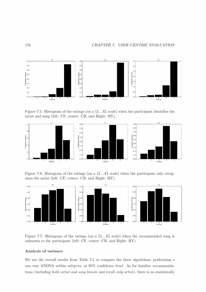
176 CHAPTER 7. USER–CENTRIC EVALUATION
Figure 7.5: Histogram of the ratings (on a [1..5] scale) when the participant identifies theartist and song (left: CF, center: CB, and Right: HY).
Figure 7.6: Histogram of the ratings (on a [1..5] scale) when the participant only recog-nises the artist (left: CF, center: CB, and Right: HY).
Figure 7.7: Histogram of the ratings (on a [1..5] scale) when the recommended song isunknown to the participant (left: CF, center: CB, and Right: HY).
Analysis of variance
We use the overall results from Table 7.1 to compare the three algorithms, performing a
one–way ANOVA within subjects, at 95% confidence level. As for familiar recommenda-
tions (including both artist and song known and recall only artist), there is no statistically
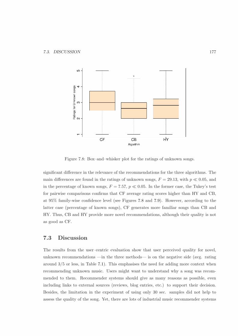
7.3. DISCUSSION 177
Figure 7.8: Box–and–whisker plot for the ratings of unknown songs.
significant difference in the relevance of the recommendations for the three algorithms. The
main differences are found in the ratings of unknown songs, F = 29.13, with p ≪ 0.05, and
in the percentage of known songs, F = 7.57, p ≪ 0.05. In the former case, the Tukey’s test
for pairwise comparisons confirms that CF average rating scores higher than HY and CB,
at 95% family-wise confidence level (see Figures 7.8 and 7.9). However, according to the
latter case (percentage of known songs), CF generates more familiar songs than CB and
HY. Thus, CB and HY provide more novel recommendations, although their quality is not
as good as CF.
7.3 Discussion
The results from the user–centric evaluation show that user perceived quality for novel,
unknown recommendations —in the three methods— is on the negative side (avg. rating
around 3/5 or less, in Table 7.1). This emphasises the need for adding more context when
recommending unknown music. Users might want to understand why a song was recom-
mended to them. Recommender systems should give as many reasons as possible, even
including links to external sources (reviews, blog entries, etc.) to support their decision.
Besides, the limitation in the experiment of using only 30 sec. samples did not help to
assess the quality of the song. Yet, there are lots of industrial music recommender systems
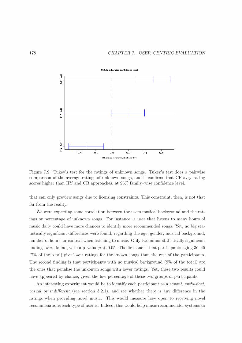
178 CHAPTER 7. USER–CENTRIC EVALUATION
Figure 7.9: Tukey’s test for the ratings of unknown songs. Tukey’s test does a pairwisecomparison of the average ratings of unknown songs, and it confirms that CF avg. ratingscores higher than HY and CB approaches, at 95% family–wise confidence level.
that can only preview songs due to licensing constraints. This constraint, then, is not that
far from the reality.
We were expecting some correlation between the users musical background and the rat-
ings or percentage of unknown songs. For instance, a user that listens to many hours of
music daily could have more chances to identify more recommended songs. Yet, no big sta-
tistically significant differences were found, regarding the age, gender, musical background,
number of hours, or context when listening to music. Only two minor statistically significant
findings were found, with a p–value p ≪ 0.05. The first one is that participants aging 36–45
(7% of the total) give lower ratings for the known songs than the rest of the participants.
The second finding is that participants with no musical background (9% of the total) are
the ones that penalise the unkonwn songs with lower ratings. Yet, these two results could
have appeared by chance, given the low percentage of these two groups of participants.
An interesting experiment would be to identify each participant as a savant, enthusiast,
casual or indifferent (see section 3.2.1), and see whether there is any difference in the
ratings when providing novel music. This would measure how open to receiving novel
recommenations each type of user is. Indeed, this would help music recommender systems to

7.3. DISCUSSION 179
Figure 7.10: Location of the three music recommendation approaches in the novelty vs.relevance axis (presented in chapter 4, Figure 4.8).
decide whether being risky or confident with the personalised recommendations. However,
with the participants data that we gatehered it was not straightforward to decide which
type of user each participant was.
Regarding recommendation approaches, the context–free and popularity agnostic CB
algorithm sometimes points in the wrong direction (it is not that easy to discriminate
between a, say, classical guitar and a harpsichord, based solely on the audio content),
and gives poor or non–sense recommendations. This leaves room for improving the audio
similarity algorithm. In this sense, the proposed hybrid approach drastically reduces the
space of possible similar tracks to those artists related to the original artist. This avoids,
most of the time, the mistakes performed by the pure CB, but on the other hand the HY
results are less eclectic than CB. CF tends to be more conservative, providing less novel
recommendations, but of higher quality, relevant to the user. Figure 7.10 summarises the
comparison of the three approaches, based on the trade–off between novelty and relevance
(presented in chapter 4, Figure 4.8).
We can envision different solutions to cope with novelty in recommender systems. The
first one is to use CF, promoting unknown artists by means of exploiting the Long Tail
popularity of the catalog and the topology of the recommendation network. Another option
180 CHAPTER 7. USER–CENTRIC EVALUATION
is switching among algorithms when needed. For instance, to avoid the cold–start problem
whilst promoting novelty, one option is to use CB or the hybrid approach, although this one
heavily relies on human resources. After a while, the system can move to a stable CF or HY
approaches. Or, we could also take into account the artist’s (or user) location in the Long
Tail, and use one or another algorithm accordingly. Furthermore, the system should be able
to change the recommendation approach according to the user’s needs. Sometimes, a user
is open to discovering new artists and songs (novelty), while sometimes she just wants to
listen to her favourites (familiarity). Detecting these modes and acting accordingly should
increase the user’s satisfaction with the system.
7.4 Limitations
To conclude, we also want to point out some limitations of the experiment. Users had
to rate songs using only a 30 second audio preview. Even though the participants could
listen to the songs repeatedly, it is not easy to rate a song the first time one listens to
it. Sometimes, one can love a song after hearing it several times, in different contexts and
moods. We could not measure this effect in the experiment. One solution could be to allow
participants to download the full songs, and then after a period of time (e.g. one week,
one month) they notify us with the total playcounts for each recommended song. Relevant
songs could be inferred from the listening habits about the recommended songs. However,
in this case a limitation is that we would collect less answers from the participants (i.e. only
the songs that were listened to at least once).
Another issue is that musical tastes from the participants were gathered from last.fm,
which is also one of the recommendation approaches used. This means that, beforehand,
the participants were used to this system and the recommendations it provides. Yet, we
decided that this music profile is more compact and reliable than asking the participant,
at the beginning of the experiment, to enter a list of her favourite artists. Furthermore,
another constraint is that only users with a last.fm account could participate in the survey.
The blind recommendation method approach —without providing any context— does
not help in assessing the relevance of the novel recommendations. It might be the case that
some of the novel songs were rated badly, but when explaining the relationships with the
user’s favourite artists, the artist biography, images, etc. the perceived quality could be
increased. In real recommender systems, blind recommendations with no explanations are
7.4. LIMITATIONS 181
useless. Why is as important as what is being recommended.
Last but not least, we are not interested on judging which recommendation method
performs the best, but on detecting the main differences among the approaches, and how
people respond to each approach. In this sense, it is not fair to compare a real system
like last.fm to the other two straight–forward plain approaches. In addition, we did not
include a fourth method, say a random recommender, that could serve us as a baseline for
the recommendations. This way, we could assess whether the three methods perform, at
least, better than the baseline. Instead, we chose to gather more ratings from the three real
methods than adding another —baseline— method in the survey.

182 CHAPTER 7. USER–CENTRIC EVALUATION

Chapter 8
Applications
This chapter presents two implemented prototypes related with music discovery and recom-
mendation. The first system, named, Searchsounds, is a music search engine based on text
keyword searches, as well as a more like this button, that allows users to discover music by
means of audio similarity. Thus, Searchsounds allows users to dig into the Long Tail, by
providing music discovery using audio content–based similarity. The second system, named
FOAFing the Music, is a music recommender system that focuses on the Long Tail of popu-
larity, promoting unknown artists. The system also provides related information about the
recommended artists, using information available on the web gathered from music related
RSS feeds.
The main difference between the two prototypes is that Searchsounds is a non–personalised
music search engine, whilst FOAFing the Music takes into account the user profile and the
listening habits to provide personalised recommendations.
8.1 Searchsounds: Music discovery in the Long Tail
SearchSounds, is a web–based music search engine that allows users to discover music using
content–based similarity. Section 8.1.1 introduces the motivations and background of the
system implemented. In section 8.1.3 we present the architecture of the system. Finally,
the last section summaries the work done and outlines the remaining work regarding the
functionality of the system.
183
184 CHAPTER 8. APPLICATIONS
8.1.1 Motivation
Nowadays, the increasing amount of available music in the World Wide Web makes very
difficult, to the user, to find music she would like to listen to. To overcome this problem,
there are some audio search engines1 that can fit the user’s needs. Some of the current
existing search engines are, nevertheless, not fully exploited because their companies would
have to deal with copyright infringing material. As general search engines, music search
engines have a crucial component: an audio crawler, that scans the web for audio files, and
also gathers related information about files (Knopke, 2004).
Syndication of Web Content
During the last years, syndication of web content —a section of a website made available for
other sites to use— has become a common practice for websites. This originated with news
and weblog sites, but nowadays is increasingly used to syndicate any kind of information.
Since the beginning of 2003, a special type of weblog, named audio weblogs (or MP3 blogs),
has become very popular. These blogs make music titles available for download. The
posted music is explained by the blog author, and usually it has links that allow users to
buy the complete album or work. Sometimes, the music is hard to find or has not been
issued in many years, and many MP3 blogs link strictly to music that is authorised for free
distribution. In other cases, MP3 blogs include a disclaimer stating that they are willing
to remove music if the copyright owner objects. Anyway, this source of semi–structured
information is a jewel for web crawlers, as it contains the user’s object of desire —the
music—, and some textual information that is referring to the audio file.
The file format used to syndicate web content is XML. Web syndication is based on
the RSS family and Atom formats. The RSS abbreviation is used to refer to the following
standards: Really Simple Syndication (RSS 2.0), Rich Site Summary (RSS 0.91 and 1.0) or
RDF Site Summary (1.0).
Of special interest are the feeds that syndicate multimedia content. These feeds publish
audiovisual information that is available on the net. An interesting example is the Media
RSS (mRSS) specification2, lead by Yahoo! and the multimedia RSS community. mRSS
1To mention a few ( accessed on September, 21st, 2008):http://audio.search.yahoo.com/,http://www.audiocrawler.com/, andhttp://www.altavista.com/audio/
2http://search.yahoo.com/mrss/

8.1. SEARCHSOUNDS: MUSIC DISCOVERY IN THE LONG TAIL 185
allows bloggers to syndicating multimedia files (audio, video, image) in RSS feeds, and adds
several enhancements to RSS enclosures. Although mRSS is not yet widely used on the net,
some websites syndicate their multimedia content following the specification3. These feeds
contain textual information, plus a link to the actual audiovisual file. As an example, listing
8.1 shows a partial RSS feed4.
<rss version="2.0"
xml:base="http: //www.ourmedia.org"
xmlns:media="http: // search.yahoo.com/mrss"
xmlns:dc="http: //purl.org/dc/elements /1.1/"
>
<channel >
<title >Example of a mRSS feed</title >
<link>http: //www.ourmedia.org/user /45801 </link>
<description >
Recently published media items from Ourmedia.org
</description >
<language >en</language >
<item>
<title >Fanky beats </title >
<link>http: //www.ourmedia.org/node /...</link>
<description >Rock music with a funky beat and electric lead
guitar riffs (...) </description >
<pubDate >Mon , 17 Apr 2007 01 :35:49 -0500</pubDate >
<dc:creator >John Brettbutter </dc:creator >
<category domain="urn:ourmedia:term:35 ">
Alternative Rock
</category >
<category domain="urn:ourmedia:term:582 ">funk</category >
<category domain="urn:ourmedia:term:727 ">guitar </category >
<enclosure url="http: // archive.org /.../ file.mp3"
length="3234212" type="application/octet -stream" />
</item>
<item>
<title >Another item</title >
...
</item>
</channel >
</rss>
Listing 8.1: Example of a media RSS feed.
3One of the most important ones is http://www.ourmedia.org4Adapted from a real example published in OurMedia website. http://www.ourmedia.org

186 CHAPTER 8. APPLICATIONS
The example shows an item with all its information: the title of the item, the description,
the publication date, the editor of the entry, and a set of categories (similar to tags, but
controlled from a given taxonomy). SearchSounds mines this information in order to retrieve
relevant audio files based on keywords.
8.1.2 Goals
The main goal of the system is to allow users to discover unknown music. For this reason,
SearchSounds mines music related information available in MP3–weblogs, and attaches tex-
tual information to the audio files. This way, users can search and retrieve music related to
the query, as well as music that sounds similar to the retrieved audio files. This exploration
mode allows users to discover music —related to his original (keyword based) query— that
would be more difficult to discover using only textual queries.
Figure 8.1 shows the relationship between the music information plane (see section 3.3),
and the information that SearchSounds uses.
8.1.3 System overview
SearchSounds exploits and mines all the music related information available from MP3–
weblogs. The system gathers editorial, cultural, and acoustic information from the crawled
audio files. The input of the system is a query composed by text keywords. From these
keywords, the system is able to retrieve a list of audio files related with the query. Each
audio file provides a link to the original weblog, and a list of similar titles. This similarity
is computed using content–based audio description. Thus, from the results of a keyword
query, a user can discover related music by navigating onto the audio similarity plane.
It is worth to mention that there is no user profiling or any kind of user representation
stored in the system. This is a limitation, as the system does not make any personalised
recommendations. However, this limitation is solved in the next prototype (explained in
section 8.2). The main components of the system are the audio crawler and the audio
retrieval system. Figure 8.2 depicts the architecture of the system.
Audio Crawler
The system has an audio spider module that crawls the web. All the gathered information
is stored into a relational database. The audio crawler starts the process from a manually
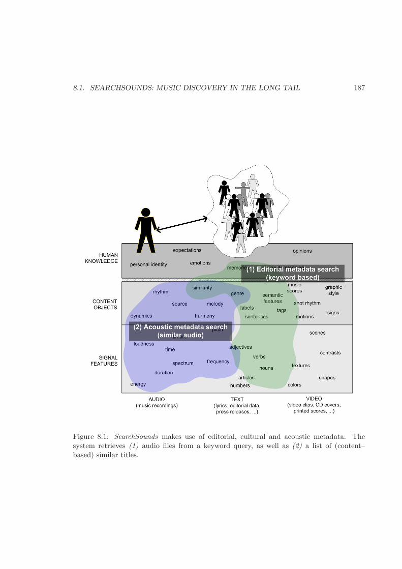
8.1. SEARCHSOUNDS: MUSIC DISCOVERY IN THE LONG TAIL 187
Figure 8.1: SearchSounds makes use of editorial, cultural and acoustic metadata. Thesystem retrieves (1) audio files from a keyword query, as well as (2) a list of (content–based) similar titles.
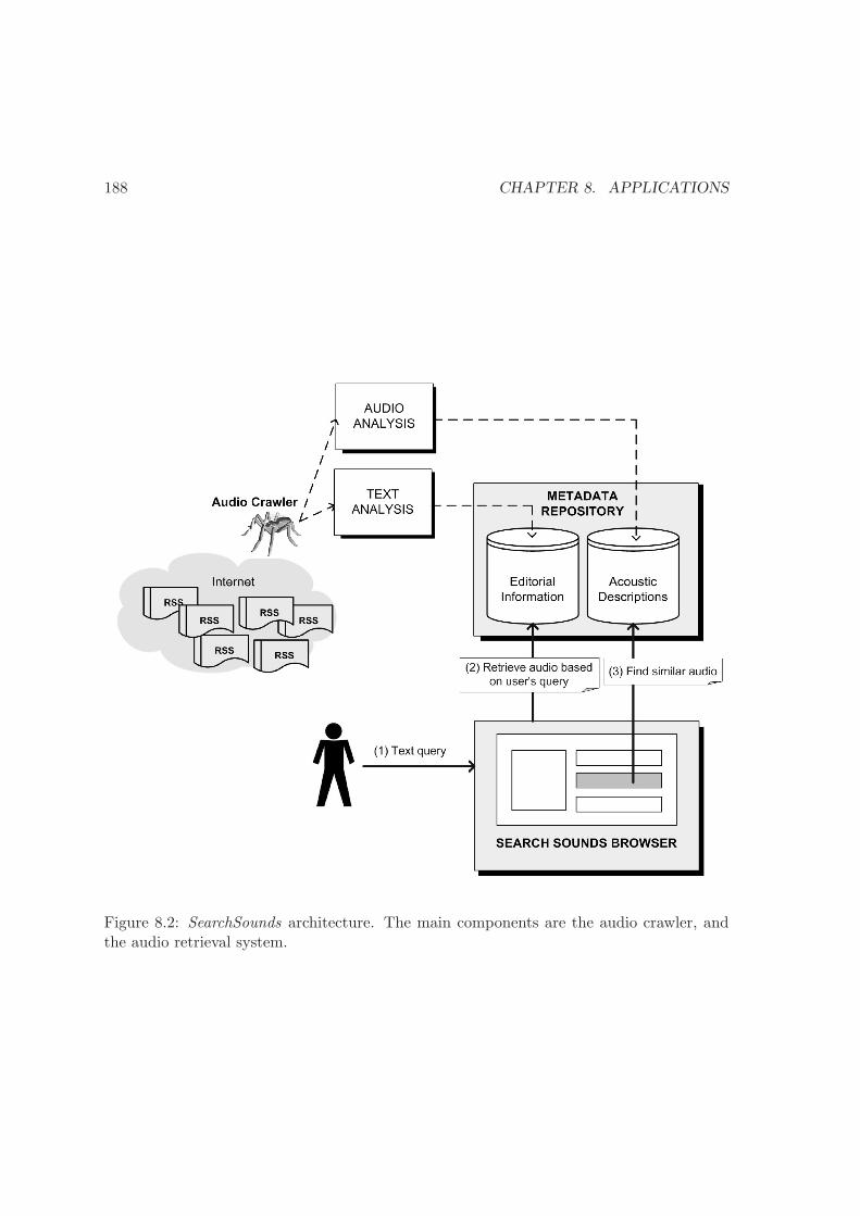
188 CHAPTER 8. APPLICATIONS
Figure 8.2: SearchSounds architecture. The main components are the audio crawler, andthe audio retrieval system.
8.1. SEARCHSOUNDS: MUSIC DISCOVERY IN THE LONG TAIL 189
selected list of RSS links (that point to MP3–blogs). Each RSS file contains a list of entries
(or items) that link to audio files. The crawler seeks for new incoming items —using the
pubDate item value and comparing with the latest entry in the database— and stores
the new information into the database. Thus, the audio crawler system has an historic
information of all the items that appeared in a feed.
From the previous RSS example (see example 8.1, presented in section 8.1.1), the audio
crawler stores the title, the content of the description, the assigned terms from the tax-
onomy (category tags), and the link to the audio file (extracted from the enclosure url
attribute).
Audio Retrieval System
The logical view of a crawled feed item can be described by the bag–of–words approach: a
document is represented as a number of unique words, with a weight (in our case, the tf/idf
function) assigned to each word (Baeza-Yates and Ribeiro-Neto, 1999). Special weights are
assigned to the music related terms, as well as the metadata (e.g ID3 tags) extracted from
the audio file. Similar to our approach, (Vembu and Baumann, 2004) presents a proposal
of modifying the weights of the terms pertaining to the musical domain.
Moreover, basic natural language processing methods are applied to reduce the size
of the item description (elimination of stopwords, and apply Porter’s stemming algorithm
(Porter, 1980)). The information retrieval (IR) model used is the classic vector model
approach, where a given document is represented as a vector in a multidimensional space
of words (each word of the vocabulary is a coordinate in the space).
The similarity function, sim(dj , q), between a query (q) and a document (dj) is based
on the cosine similarity, using TF/IDF weighting function (already presented in section
2.5.4). Our approach is well suited not only for querying via artists’ or songs’ names, but
for more complex keyword queries such as: “funky guitar riffs” or “traditional Irish tunes”.
The retrieval system outputs the documents (i.e. feed entries) that are relevant to the
user’s query, ranked by the similarity function. Figure 8.3 depicts the retrieved audio files
for “traditional Irish music” query.
Based on the results obtained from the user’s textual query, the system allows users
to find similar titles using content–based audio similarity. Each link to an audio file has a
“Find similar” button that retrieves the most similar audio files, based on a set of low and
mid-level audio descriptors. These descriptors are extracted from the audio and represent
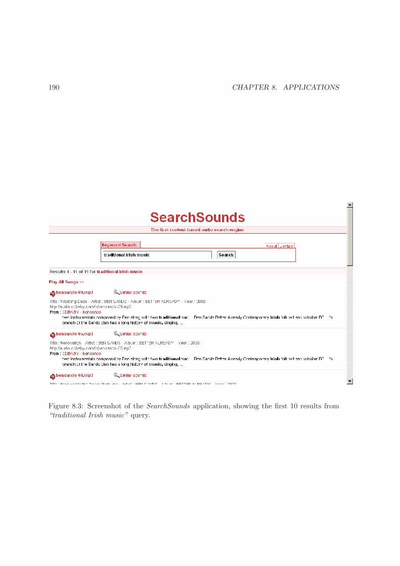
190 CHAPTER 8. APPLICATIONS
Figure 8.3: Screenshot of the SearchSounds application, showing the first 10 results from“traditional Irish music” query.

8.2. FOAFING THE MUSIC: MUSIC RECOMMENDATION IN THE LONG TAIL 191
properties such as: rhythm, harmony, timbre and instrumentation, intensity, structure and
complexity (Cano et al., 2005).
This exploration via browsing allows users to discover music —related to his original
(keyword based) query— that would be more difficult to discover by using textual queries
only. There is an analogy between this type of navigation and, for example, Google’s “find
web pages that are similar to a given HTML page”. In our case, similarity among items
are based on audio similarity, whereas Google approach is based on the textual content of
the HTML page. Still, both browsing approaches are based on the content analysis of the
retrieved object.
8.1.4 Summary
We developed a web–based audio crawler that focuses on MP3–weblogs. Out of the crawling
process, each feed item is represented as a text document, containing the content of the
item, as well as the links to the audio files. Then, classic text retrieval system outputs
relevant feed items related to the user’s query. Furthermore, a content–based navigation
allows users to browse through the retrieved items and discover new music and artists using
audio similarity.
Ongoing work includes the automatic extraction of music related tags (i.e. guitar, rock,
70’s) from the text, as well as applying autotagging to incoming audio files; using audio
content–based similarity (Sordo et al., 2007). We also plan to add relevance feedback to
tune the system and get more accurate results, specially for the content–based similarity.
The system is available at http://www.searchsounds.net.
8.2 FOAFing the Music: Music recommendation in the Long
Tail
Now we present the second of the two prototypes developed. It is a music recommender
system, named FOAFing the Music, that allows users to discover a wide range of music
located along the Long Tail. The system exploits music related information that is being
syndicated (as RSS feeds) on thousands of websites. Using the crawled information, the
system is able to filter it and recommend it to the user, according to her profile and listening
habits.
192 CHAPTER 8. APPLICATIONS
8.2.1 Motivation
The World Wide Web has become the host and distribution channel for a broad variety of
digital multimedia assets. Although the Internet infrastructure allows simple straightfor-
ward acquisition, the value of these resources lacks powerful content management, retrieval
and visualisation tools. Music content is no exception: although there is a sizeable amount
of text–based information related to music (album reviews, artist biographies, etc.) this
information is hardly ever associated with the objects it refers to, that being the music files
themselves (MIDI or audio). Moreover, music is an important vehicle for communicating
to other people something relevant about our personality, history, etc.
There is a clear interest in the Semantic Web field in creating a Web of machine–readable
homepages describing people, the links among them, and the things they create and do.
The FOAF (Friend Of A Friend) project5 provides conventions and a language to describe
homepage–like content and social networks. The FOAF vocabulary provides properties and
classes for describing common features of people and their social networks. FOAF is based
on the RDF/XML6 vocabulary.
We foresee that with a complete user’s FOAF profile, our system would get a better
representation of the user’s musical needs. On the other hand, the RSS vocabulary7 allows
systems one to syndicate Web content on the Internet. Syndicated content includes data
such as news, event listings, headlines, project updates, as well as music related information,
such as new music releases, album reviews, podcast sessions, and upcoming gigs.
To our knowledge, nowadays it does not exist any system that recommends items to a
user, based on her FOAF profile. Yet, it is worth to mention the FilmTrust system8. It is
a part of a research study aimed to understanding how social preferences might help web
sites to present information in a more useful way (Golbeck and Parsia, 2005). The system
collects user reviews and ratings about movies, and holds them into the user’s FOAF profile
(Golbeck, 2005).
5http://www.foaf-project.org6http://www.w3.org/RDF7http://web.resource.org/rss/1.0/8http://trust.mindswap.org/FilmTrust

8.2. FOAFING THE MUSIC: MUSIC RECOMMENDATION IN THE LONG TAIL 193
Figure 8.4: FOAFing the Music and the music information plane.
194 CHAPTER 8. APPLICATIONS
8.2.2 Goals
The main goal of the FOAFing the Music system is to recommend, to discover and to explore
music content; based on user profiling (via FOAF descriptions), context based information
(extracted from music related RSS feeds), and content based descriptions (automatically
extracted from the audio itself). All of that being based on a common ontology that
describes the musical domain.
Figure 8.4 shows the relationship between the music information plane, and the dif-
ferent sources of metadata that the system exploits. Compared to the first prototype
(Searchsounds), Foafing the Music holds a user profile representation, based on the FOAF
initiative (already presented in section 3.2). A FOAF user profile allows to filter music
related information according to user’s preferences.
8.2.3 System overview
The overview of the Foafing the Music system is depicted in Fig. 8.5. The system is divided
in two main components, that is (i) how to gather data from external third party sources
(presented in section 8.2.3), and (ii) how to recommend music to the user based on the
crawled data, and the semantic description of the music titles (section 8.2.3).
Gathering music related information
Personalised services can raise privacy concerns due to the acquisition, storage and applica-
tion of sensitive personal information (Perik et al., 2004). In our system, information about
the user is not stored in the system in any way. Instead, the system has only a link pointing
to the user’s FOAF profile (often a link to a Livejournal account). Thus, the sensitivity
of this data is up to the user, not to the system. Users’ profiles in Foafing the Music are
distributed over the net.
Regarding music related information, our system exploits the mashup approach. The
system uses a set of public available APIs and web services sourced from third party websites.
This information can come in any of the different RSS formats (v2.0, v1.0, v0.92 and Yahoo!
Media RSS), as well as in the Atom format. Thus, the system has to deal with syntactically
and structurally heterogeneous data. Moreover, the system keeps track of all the new items
that are published in the feeds, and stores the new incoming data in a historic relational
database. Input data of the system is based on the following information sources:
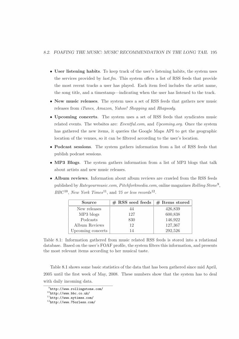
8.2. FOAFING THE MUSIC: MUSIC RECOMMENDATION IN THE LONG TAIL 195
• User listening habits. To keep track of the user’s listening habits, the system uses
the services provided by last.fm. This system offers a list of RSS feeds that provide
the most recent tracks a user has played. Each item feed includes the artist name,
the song title, and a timestamp—indicating when the user has listened to the track.
• New music releases. The system uses a set of RSS feeds that gathers new music
releases from iTunes, Amazon, Yahoo! Shopping and Rhapsody.
• Upcoming concerts. The system uses a set of RSS feeds that syndicates music
related events. The websites are: Eventful.com, and Upcoming.org. Once the system
has gathered the new items, it queries the Google Maps API to get the geographic
location of the venues, so it can be filtered according to the user’s location.
• Podcast sessions. The system gathers information from a list of RSS feeds that
publish podcast sessions.
• MP3 Blogs. The system gathers information from a list of MP3 blogs that talk
about artists and new music releases.
• Album reviews. Information about album reviews are crawled from the RSS feeds
published by Rateyourmusic.com, Pitchforkmedia.com, online magazines Rolling Stone9,
BBC 10, New York Times11, and 75 or less records12.
Source # RSS seed feeds # Items stored
New releases 44 426,839MP3 blogs 127 600,838Podcasts 830 146,922
Album Reviews 12 127,367Upcoming concerts 14 292,526
Table 8.1: Information gathered from music related RSS feeds is stored into a relationaldatabase. Based on the user’s FOAF profile, the system filters this information, and presentsthe most relevant items according to her musical taste.
Table 8.1 shows some basic statistics of the data that has been gathered since mid April,
2005 until the first week of May, 2008. These numbers show that the system has to deal
with daily incoming data.
9http://www.rollingstone.com/10http://www.bbc.co.uk/11http://www.nytimes.com/12http://www.75orless.com/

196 CHAPTER 8. APPLICATIONS
Figure 8.5: Architecture of the Foafing the Music system.
An ontology is an explicit and formal specification of a conceptualisation Gruber (1993).
In general, an ontology describes formally a domain of discourse. The requeriments for
Ontology languages are: a well-defined syntax, a formal semantics, and a reasoning support
that checks the consistency of the ontology, checks for unintended relationships between
classes, and automatically classifies instances in classes.
The Web Ontology Language (OWL) has a richer vocabulary description language for
describing properties and classes than RDFS. OWL has relations between classes, cardinal-
ity, equality, characteristics of properties and enumerated classes. The OWL language is
build on RDF and RDFS, and uses RDF/XML syntax. OWL documents are, then, RDF
documents.
On the other hand, we have defined a simple music recommendation OWL DL ontol-
ogy (http://foafing-the-music.iua.upf.edu/music-ontology#) that describes some
basic properties of the artists and music titles, as well as some descriptors automatically
extracted from the audio files (e.g. tonality, rhythm, moods, music intensity, etc.). In
(Garcia and Celma, 2005) we propose a way to map our ontology and the Musicbrainz
ontology, onto the MPEG-7 standard, which acts as an upper-ontology for multimedia
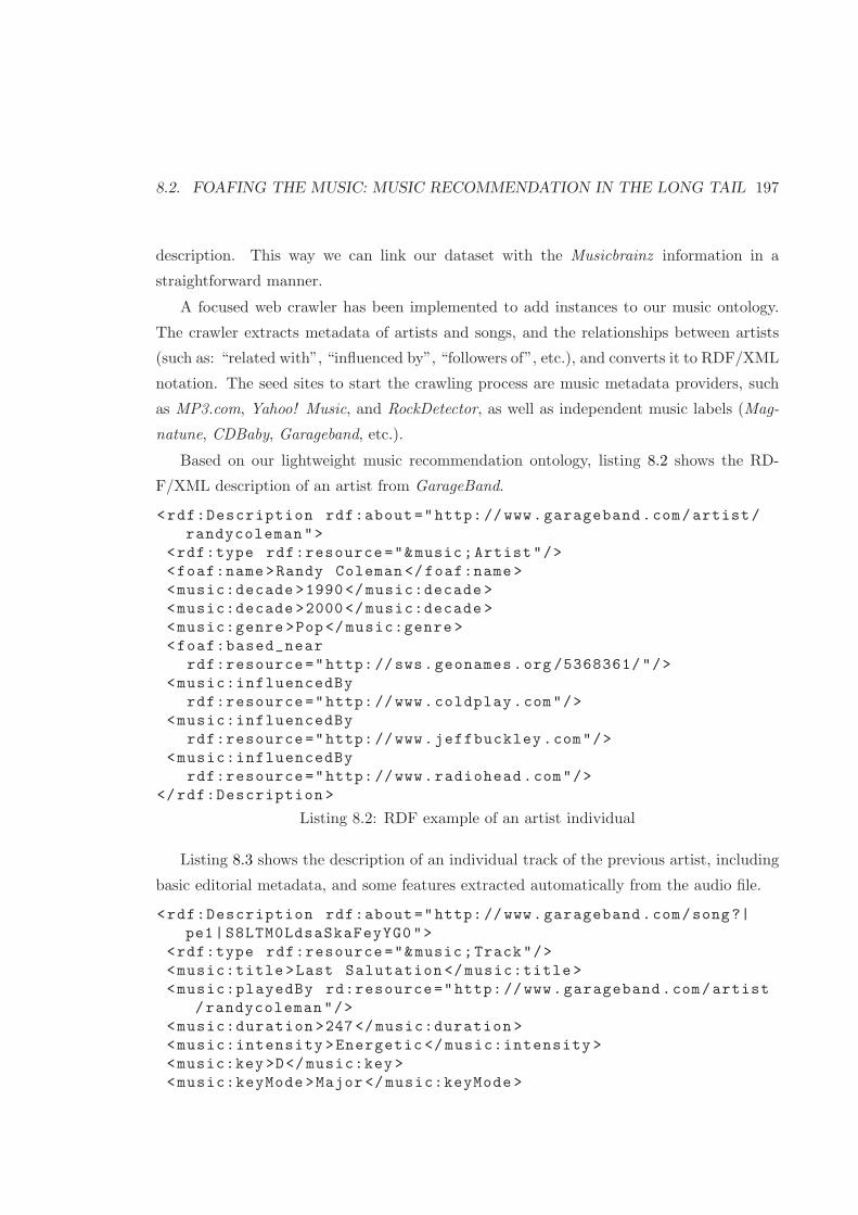
8.2. FOAFING THE MUSIC: MUSIC RECOMMENDATION IN THE LONG TAIL 197
description. This way we can link our dataset with the Musicbrainz information in a
straightforward manner.
A focused web crawler has been implemented to add instances to our music ontology.
The crawler extracts metadata of artists and songs, and the relationships between artists
(such as: “related with”, “influenced by”, “followers of”, etc.), and converts it to RDF/XML
notation. The seed sites to start the crawling process are music metadata providers, such
as MP3.com, Yahoo! Music, and RockDetector, as well as independent music labels (Mag-
natune, CDBaby, Garageband, etc.).
Based on our lightweight music recommendation ontology, listing 8.2 shows the RD-
F/XML description of an artist from GarageBand.
<rdf:Description rdf:about="http: //www.garageband.com/artist/
randycoleman">
<rdf:type rdf:resource="&music;Artist"/>
<foaf:name >Randy Coleman </foaf:name >
<music:decade >1990</music:decade >
<music:decade >2000</music:decade >
<music:genre >Pop</music:genre >
<foaf:based_near
rdf:resource="http: //sws.geonames.org /5368361/"/>
<music:influencedBy
rdf:resource="http: //www.coldplay.com"/>
<music:influencedBy
rdf:resource="http: //www.jeffbuckley.com"/>
<music:influencedBy
rdf:resource="http: //www.radiohead.com"/>
</rdf:Description >
Listing 8.2: RDF example of an artist individual
Listing 8.3 shows the description of an individual track of the previous artist, including
basic editorial metadata, and some features extracted automatically from the audio file.
<rdf:Description rdf:about="http: //www.garageband.com/song?|
pe1|S8LTM0LdsaSkaFeyYG0">
<rdf:type rdf:resource="&music;Track"/>
<music:title >Last Salutation </music:title >
<music:playedBy rd:resource="http: //www.garageband.com/artist
/randycoleman"/>
<music:duration >247</music:duration >
<music:intensity >Energetic </music:intensity >
<music:key >D</music:key >
<music:keyMode >Major </music:keyMode >
198 CHAPTER 8. APPLICATIONS
<music:tonalness >0.84</music:tonalness >
<music:tempo >72</music:tempo >
</rdf:Description >
Listing 8.3: Example of a track individual
These individuals are used in the recommendation process, to retrieve artists and songs
related with the user’s musical taste.
Providing music recommendation
This section explains the music recommendation process, based on all the information that
has continuously been gathered from the RSS feeds and the crawler. Music recommenda-
tions, in the Foafing the Music system, are generated according to the following steps:
1. Get music related information from user’s FOAF interests, and listening habits from
last.fm,
2. Detect artists and bands,
3. Compute similar artists, and
4. Rate the results by relevance, according to the user’s profile.
To gather music related information from a FOAF profile, the system extracts the
information from the FOAF interest property (if dc:title is given then it gets its value,
otherwise it gathers the text from the <title> tag of the HTML resource).
<foaf:interest
rdf:resource="http: //www.tylaandthedogsdamour .com/"
dc:title="The Dogs d’Amour" />
Listing 8.4: Example of a FOAF interest with a given dc:title.
The system can also extract information from a user’s FOAF interest that includes the
artist description based on the general Music Ontology (Giasson and Raimond, 2007).
Based on the music related information gathered from the user’s profile and listening
habits, the system detects the artists and bands that the user is interested in, by doing a
SPARQL query to the artist RDF repository. Once the user’s artists have been detected,
artist similarity is computed. This process is achieved by exploiting the RDF graph of
artists’ relationships (e.g. influenced by, followers of, worked with, etc.), as shown in Listing
8.2.
8.2. FOAFING THE MUSIC: MUSIC RECOMMENDATION IN THE LONG TAIL 199
The system offers two ways of recommending music information. On the one hand, static
recommendations are based on the favourite artists encountered in the FOAF profile. We
assume that a FOAF profile would be rarely manually updated or modified. On the other
hand, dynamic recommendations are based on user’s listening habits, which are updated
much more often than the user’s profile. Following this approach a user can discover a wide
range of new music and artists on a daily basis.
Once the recommended artists have been computed, Foafing the Music filters music
related information coming from the gathered music information (see section 8.2.3) to:
• Get new music releases from iTunes, Amazon, Yahoo Shopping, etc.
• Download (or stream) audio from MP3–blogs and Podcast sessions,
• Create, automatically, XSPF13 playlists based on audio similarity,
• View upcoming gigs happening near to the user’s location, and
• Read album reviews.
Syndication of the website content is done via an RSS 1.0 feed. For most of previous
functionalities, there is a feed subscription option to get the results.
Usage data
Since its inception in August 2005, the system has an average of 60 daily unique accesses,
from more than 4,000 registered users, including casual users that try the demo option.
More than half of the users automatically created an account using an external FOAF
profile (most of the times, around 70%, the profile came from their Livejournal FOAF
account). Also, more than 65% of the users add her last.fm account, so we can use their
listening habits from last.fm. Figure 8.6 shows the number of logins over time, since August
2005 till July 2008. The peaks are clearly correlated with related news about the project
(e.g. local TV and radio interviews, and reviews on the web).
8.2.4 Summary
We have proposed a system that filters music related information, based on a given user’s
FOAF profile and her listening habits. A system based on FOAF profiles and user’s listening
13http://www.xspf.org/. XSPF is a playlist format based on XML syntax
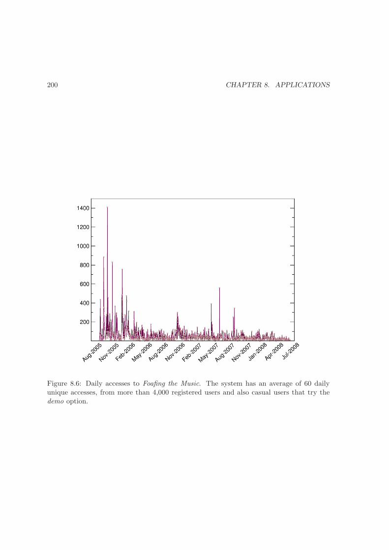
200 CHAPTER 8. APPLICATIONS
Figure 8.6: Daily accesses to Foafing the Music. The system has an average of 60 dailyunique accesses, from more than 4,000 registered users and also casual users that try thedemo option.
8.2. FOAFING THE MUSIC: MUSIC RECOMMENDATION IN THE LONG TAIL 201
habits allows the system to “understand” a user in two complementary ways; psychologi-
cal factors—personality, demographic preferences, social relationships—and explicit musical
preferences. In the music field, we expect that filtering information about new music re-
leases, artists’ interviews, album reviews, and so on, can improve user satisfaction as it
provides the context and needed information to backup the system’s recommendations.
Describing music assets is a crucial task for a music recommender system. The success of
a music recommender can depend on the accuracy and level of detail of the musical objects,
and its links within a user profile. Furthermore, we formalise into an ontology the basic
musical concepts involved in the recommendation process. Linking these musical objects
with the user profile eases the recommendation process.
Furthermore, high–level musical descriptors can increase the accuracy of content re-
trieval, as well as provide better personalised recommendations. Thus, going one step
beyond, it would be desirable to combine mid–level acoustic features with as much editorial
and cultural metadata as possible. From this combination, more sophisticated inferences
and semantic rules would be possible. These rules could derive hidden high–level metadata
that could be easily understood by the end–user, also enhancing their profiles. Since the
existence of the general Music Ontology (MO) (Giasson and Raimond, 2007), we foresee
that linking our recommendation ontology with it, as well as using all the linked informa-
tion available in the Web of Data14, we can improve our recommender, becoming a truly
semantically–enhanced music recommender.
Foafing the Music is accessible through http://foafing-the-music.iua.upf.edu.
14See http://linkeddata.org/.

202 CHAPTER 8. APPLICATIONS

Chapter 9
Conclusions and Further Research
Research in recommender systems is multidisciplinary. It includes several areas, such as:
search and filtering, data mining, personalisation, social networks, text processing, complex
networks, user interaction, information visualisation, signal processing, and domain specific
models, among others. Furthermore, current research in recommender systems has strong
industry impact, resulting in many practical applications.
In this thesis we focused on the central pillar of any Recommender System: the sim-
ilarity among objects. We proposed new approaches to evaluate the effectiveness of the
recommendations in the music domain. Our goal is to promote the discovery of items via
the functionality offered by recommender systems. In this sense, novelty and relevance of
recommendations are the two most important aspects. We make use of the Long Tail shape
to model the popularity bias that exists in any recommender system, and use this data to
recommend unknown items, hidden in the tail of the popularity curve. Our experience is
that using the F (x) function to model the Long Tail curve we get more accurate results
that fitting the curve to well-known distributions, such as power–law or log–normal (Kilkki,
2007).
We have an overwhelming number of choices about which music to listen to. As stated
in (Schwartz, 2005), we —as consumers— often become paralysed and doubtful when facing
the overwhelming number of choices. The main problem, then, is the awareness of content
in the tail, not the actual access to the content. Here is where personalised filters and rec-
ommender systems enter as part of the solution. Effective recommendation systems should
promote novel and relevant material (non–obvious recommendations), taken primarily from
the tail of a popularity distribution.
203

204 CHAPTER 9. CONCLUSIONS AND FURTHER RESEARCH
9.1 Summary of the Research
This thesis has presented a number of novel ideas that address existing limitations in recom-
mender systems, and the lack of systematic methods to evaluate the novelty and perceived
quality of recommendations. Furthermore, two real web–based systems have been imple-
mented to demonstrate the ideas derived from the theoretical work. The main products of
the thesis are:
1. A novel user–agnostic evaluation method for recommender systems, based on the
analysis of the item (or user) similarity network, and the combination with the items’
popularity, using the Long Tail curve.
2. A user–centric evaluation, based on the immediate feedback of the provided recom-
mendations, that measures the user’s perceived quality and novelty factor of the rec-
ommendations.
3. A music search engine, named Searchsounds, that allows users to discover unknown
music that is available on music related blogs.
4. A system prototype, named FOAFing the music, that provides music recommendation
based on the user preferences and listening habits.
The first two results are scientific, whilst the third and fourth contributions are more
engineering and industry oriented.
9.1.1 Scientific contributions
A network–based evaluation method for recommender systems
We have formulated a network–based evaluation method for recommender systems, based
on the analysis of the item (or user) similarity network, combined with item popularity.
This method has the following advantages:
1. It measures the novelty component of a recommendation algorithm.
2. It models the item popularity curve.
3. It combines both the complex network and the item popularity analysis to determine
the underlying characteristics of the recommendation algorithm.
4. It does not require any user intervention in the evaluation process.
9.1. SUMMARY OF THE RESEARCH 205
We have applied the network–based analysis to two different similarity graphs; for artists,
and users. The results from the artist network analysis show that the last.fm social–based
recommender tends to reinforce popular artists, at the expense of discarding less–known
music. Thus, the popularity effect derived from the community of users has consequences
in the recommendation network. This reveals a somewhat poor discovery ratio when just
browsing through the network of similar music artists. Allmusic.com expert–based rec-
ommendations are more expensive to create, and also have a smaller Long Tail coverage,
compared to automatically generated recommendations like collaborative filtering or audio
content–based similarity. Regarding popularity, the hubs in the expert network are com-
prised of mainstream music. Our guess is that the editors connect long tail artists with
the most popular ones, either for being influential or because many bands are considered
followers of these mainstream artists. An audio content–based similarity network is not
affected by the popularity bias of the artists, however it is prone to the musical genre biases
of the collection, where the predominant genres includes most of the similar artists. The
main problem of audio content–based systems is the assumption that just because two songs
sound similar, any user will like both of them. It is very unlikely that a user will love both a
Franz Schubert ’s piano sonata, and a Meat Loaf piano ballad (such as “Heaven Can Wait”)
just because the two contain a prominent piano melody.
The results from the user network analysis show that user similarity network derived
from collaborative filtering resembles a social network, whilst the network derived from au-
dio content–based similarity has the properties of a hierarchy, where a few nodes connect
small clusters. The authorities in the CB network are the users that listen to more music,
independently of the quality or popularity of the music they listen to. Contrastingly, the
authorities in the CF network are the users that listen to more mainstream music. These
considerations have a big impact on recommendation algorithms that compute recommen-
dations by means of user similarity and neighbourhood information.
A user–based evaluation method for recommender systems
Our proposed evaluation measures the user’s perceived quality and novelty of the recom-
mendations. The user–centric evaluation approach has the following advantages:
1. It measures the novelty factor of a recommendation algorithm considering the user’s
knowledge of the items.
206 CHAPTER 9. CONCLUSIONS AND FURTHER RESEARCH
2. It measures the perceived quality (e.g., like it or not) of the recommendations.
3. Users provide immediate feedback to the evaluation system, so the algorithm can
adapt accordingly.
This method complements the previous, user–agnostic, network–based evaluation ap-
proach. We use the user–centric method to evaluate and compare three different music
recommendation approaches. In this experiment, 288 subjects rated the recommendations
in terms of novelty (i.e., does the user know the recommended song/artist? ), and relevance
(i.e., does the user like the recommended song? ).
The results from the music recommendation survey show that, in general, users’ per-
ceived quality for novel recommendations is neutral or negative (mean rating around 3/5
or less). This emphasises the need for adding context when recommending unknown music.
Recommender systems should give as many reasons as possible to support their decisions.
In terms of algorithms, the rating scores for the last.fm social–based approach are higher
than those for the hybrid and pure audio content–based similarity. However, the social–
based recommender generates more familiar (less novel) songs than CB and HY. Thus,
content–based and hybrid approaches provide more novel recommendations, although their
quality is not as good as the ones from last.fm.
9.1.2 Industrial contributions
FOAFing the Music: a music recommendation system
The system prototype, named FOAFing the Music, provides music recommendation based
on the user preferences and listening habits. The main goal of FOAFing the Music is
to recommend, to discover and to explore music content via user profiling, context–based
information (extracted from music related RSS feeds), and content–based descriptions (au-
tomatically extracted from the audio itself). The system has an average of 60 daily unique
accesses, from more than 4,000 registered users and also casual users that try the demo
option. FOAFing the music allows users to:
1. get new music releases from iTunes, Amazon, Yahoo Shopping, etc.
2. download (or stream) audio from MP3–blogs and Podcast sessions,
3. discover music with radio–a–la–carte (i.e., personalised playlists),
4. view upcoming nearby concerts, and
9.2. LIMITATIONS AND FURTHER RESEARCH 207
5. read album reviews.
Since the existence of the general Music Ontology (MO) (Giasson and Raimond, 2007),
we foresee that linking our recommendation ontology with it, as well as exploiting all the
linked information available in the Web of Data1, we can improve our system, becoming a
truly semantically–enhanced music recommender.
Searchsounds: a music search engine
We have implemented a music search engine, named Searchsounds, that allows users to
discover unknown music mentioned on music–related blogs. Searchsounds provides keyword
based search, as well as the exploration of similar songs using audio similarity. The system
allows users to dig into the Long Tail, by providing music discovery using audio content–
based similarity, that could not be easily retrieved using classic text retrieval techniques.
Over 400,000 audio files are currently indexed, using both text and audio features.
Ongoing work includes the automatic extraction of music related tags (i.e. guitar, rock,
70’s) from the text, as well as applying autotagging to incoming audio files; using audio
content–based similarity (Sordo et al., 2007).
9.2 Limitations and Further Research
Dynamic versus static data
It goes without saying that there are many ways in which the work presented in this thesis
could be extended or improved. One of the main limitations of our approach is that it
is not dynamic. We work with a snapshot of the item (or user) similarity network, and
the analysis is based on this data. However, the recommendation network dynamics is
an important aspect of a recommender system. Users’ taste change over time, and so it
does the similarity among items. Further work in this area would include a detailed study
of a dynamic model in the network —including trend and hype–item detection— and a
comparison with the stationary model.
1See http://linkeddata.org/.

208 CHAPTER 9. CONCLUSIONS AND FURTHER RESEARCH
Domain specific
The work done has been applied only to music recommendation. Even though we did not
use any domain–specific metrics in the network–centric evaluation, our findings cannot be
directly extrapolated to other domains. Future work includes extending the network–centric
experiments to other domains, such as movie recommendation using the Netflix dataset.
Besides, the user–centric evaluation contains a lot of particularities from the music
recommendation domain. In other domains (e.g., movies, books, or travels), explicit user
feedback about the recommended items cannot be provided in real–time. Furthermore,
our music recommendation survey design is based on providing blind recommendations.
Future work includes comparing our results with a new experiment that provides contextual
information and transparency about the music being recommended. The related question is
whether the ratings of novel items increase (i.e., perceived as better quality) when providing
more information about the recommended items.
User evaluation
In our user–centric evaluation we could not classify a participant into the four type of
listeners (savant, enthusiasts, casuals and indifferents). In fact, it would be interesting
to look at recommendation evaluations through the lense of the four types of listeners.
The type and utility of recommendations varies greatly depending on the type of user.
When testing against the general population —since most listeners fall into the casual or
indifferent bucket— recommenders that appeal to these types of listeners would score well
when compared to recommenders that are designed for the enthusiast or savant. However,
enthusiasts and savants are likely to be much more active consumers, so from an economic
point of view, there may be more value targeting them. Recommenders for savants and
enthusiasts would probably favour novelty and long tail content, while recommendations
for a casual listener would probably favour low–risk exploration. Indeed, a new task for
music recommenders could be to help casual listeners appreciate diversity and exploration
to unknown content.
User understanding
User understanding is another important aspect when providing personalised recommen-
dations. Our approach to model a user profile is a rather simple list of preferred artists.

9.3. OUTLOOK 209
Extending the user profile model, adding relevant and contextual information, would allow
recommender systems to have a better understanding of the user.
Ideally, a recommender system should provide different and personalised recommenda-
tions for a given item. That is, when visiting the Beatles’ White Album in Amazon store,
the system should present the list of recommendations according to the user profile. De-
pending on the user’s taste, the system should stress the pop side of the band, whilst in
other situations it could promote the more psychedelic or experimental music they did. On-
going work by Lamere and Maillet (2008) is aligned with this idea. They have implemented
a prototype system that creates transparent, steerable recommendations. Users can modify
the list of recommended items by changing the seed artist’s tag cloud.
Recommendations with no explanation
Blind recommendations do not provide any context nor explanation. Thus, it does not help
in assessing the relevance of novel recommendations. It might be the case that some novel
songs recommended are perceived as non–relevant, but when explaining the ties with the
user profile the perceived quality could be increased. In fact, why is as important as what
is being recommended. Again, Lamere and Maillet (2008) is a novel example of a system
that gives transparent explanations about the provided recommendations.
9.3 Outlook
We are witnessing an explosion of practical applications coming from MIR research: music
identification systems, music recommenders and playlist generators, music search engines,
etc. This is just the beginning2. A few years ago, music was a key factor in taking the
Internet from its text–centered origins to being a complete multimedia environment. Music
might do the same for the next web generation. The “Celestial Jukebox” is about to become
a reality.
2A detailed list of research MIR systems are available at http://mirsystems.info/

210 CHAPTER 9. CONCLUSIONS AND FURTHER RESEARCH
Publications
2008
1. Oscar Celma and Perfecto Herrera. “A new approach to evaluating novel recom-
mendations”. In ACM Conference on Recommender Systems, Lausanne, Switzerland,
2008.
2. Oscar Celma and Pedro Cano. “From hits to niches? or how popular artists can
bias music recommendation and discovery”. In 2nd Workshop on Large-Scale Recom-
mender Systems and the Netflix Prize Competition (ACM KDD), Las Vegas, USA,
2008.
3. Oscar Celma and Xavier Serra. “Foafing the music: Bridging the semantic gap in
music recommendation”. Web Semantics: Science, Services and Agents on the World
Wide Web, 6(4):250–256, 2008.
4. Oscar Celma and Yves Raimond. “Zempod: A semantic web approach to podcast-
ing”. Journal of Web Semantics, 6(2):162–169, 2008.
5. Massimiliano Zanin, Pedro Cano, Javier M. Buldu, and Oscar Celma. “Complex
networks in recommendation systems”. In Proceedings of the 2nd WSEAS Interna-
tional Conference on Computer Engineering and Applications, Acapulco, Mexico, In
Electrical And Computer Engineering, World Scientific Advanced Series, 2008
6. Roberto Garcıa, Chrisa Tsinaraki, Oscar Celma, and Stavros Christodoulakis. “Mul-
timedia Content Description using Semantic Web Languages” book. Chapter 2.
Springer–Verlag, 2008.
7. Mohamed Sordo, Oscar Celma, Martın Blech, and Enric Guaus. “The quest for
musical genres: Do the experts and the wisdom of crowds agree?” In 9th International
Conference on Music Information Retrieval, Philadelphia, USA, 2008.
211
212 CHAPTER 9. CONCLUSIONS AND FURTHER RESEARCH
2007
8. Oscar Celma, Stamatia Dasiopoulou, Michael Hausenblas, Suzanne Little, Chrisa
Tsinaraki, Raphael Troncy. “MPEG-7 and the Semantic Web”. W3C Technical
report, 2007.
9. Juyong Park, Oscar Celma, Markus Koppenberger, Pedro Cano, and Javier M.
Buldu. “The social network of contemporary popular musicians”. International Jour-
nal of Bifurcation and Chaos (IJBC), 17:2281–2288, 2007.
10. Raphael Troncy, Oscar Celma, Suzanne Little, Roberto Garcıa, and Chrisa Tsi-
naraki. “MPEG-7 based multimedia ontologies: Interoperability support or interop-
erability issue?” In 1st Workshop on Multimedia Annotation and Retrieval enabled
by Shared Ontologies, Genova, Italy, 2007.
11. Susanne Boll, Tobias Burger, Oscar Celma, Christian Halaschek-Wiener, and Erik
Mannens. “Multimedia vocabularies on the Semantic Web”. W3C Technical report,
2007.
12. Mohamed Sordo, Cyril Laurier, and Oscar Celma. “Annotating music collections:
how content-based similarity helps to propagate labels”. In 8th International Confer-
ence on Music Information Retrieval, Vienna, Austria, 2007.
2006
13. Oscar Celma. “Foafing the music: Bridging the semantic gap in music recommen-
dation”. In 5th International Semantic Web Conference (ISWC), Athens, GA, USA,
2006.
14. Oscar Celma, Pedro Cano, and Perfecto Herrera. “Search sounds: An audio crawler
focused on weblogs”. In 7th International Conference on Music Information Retrieval
(ISMIR), Victoria, Canada, 2006.
15. Oscar Celma, Perfecto Herrera, and Xavier Serra. “Bridging the music semantic
gap”. In 1st International conference on Semantics And digital Media Technology
(SAMT), Athens, Greece, 2006.
16. Pedro Cano, Oscar Celma, Markus Koppenberger, and Javier M. Buldu. “Topology
of music recommendation networks”. Chaos An Interdisciplinary Journal of Nonlinear
Science, 16, 2006.
9.3. OUTLOOK 213
17. Vegard Sandvold, Thomas Aussenac, Oscar Celma, and Perfecto Herrera. “Good
vibrations: Music discovery through personal musical concepts”. In 7th International
Conference on Music Information Retrieval (ISMIR), Victoria, Canada, 2006.
2005
18. Oscar Celma, Miguel Ramırez, and Perfecto Herrera. “Foafing the music: A music
recommendation system based on rss feeds and user preferences”. In 6th International
Conference on Music Information Retrieval (ISMIR), London, UK, 2005.
19. Oscar Celma, Miguel Ramırez, and Perfecto Herrera. “Getting music recommenda-
tions and filtering newsfeeds from foaf descriptions”. In 1st Workshop on Scripting
for the Semantic Web co-located with the 2nd European Semantic Web Conference),
Heraklion, Greece, 2005.
20. Roberto Garcıa and Oscar Celma. “Semantic integration and retrieval of multimedia
metadata”. In 2nd European Workshop on the Integration of Knowledge, Semantic
and Digital Media, Galway, Ireland, 2005.
21. Pedro Cano, Oscar Celma, Markus Koppenberger, and Javier M. Buldu. “The
topology of music artists’ graphs”. In XIII Congreso de Fısica Estadistica, Madrid,
SPAIN, 2005.
22. P. Herrera, Oscar Celma, J. Massaguer, P. Cano, E. Gomez, F. Gouyon, M. Kop-
penberger, D. Garca, J. G. Mahedero, and N. Wack. “Mucosa a music content se-
mantic annotator”. In 6th International Conference on Music Information Retrieval
(ISMIR), London, UK, 2005.
23. P. Cano, M. Koppenberger, N. Wack, J. G. Mahedero, J. Masip, Oscar Celma,
D. Garcia, E. Gomez, F. Gouyon, E. Guaus, P. Herrera, J. Massaguer, B. Ong, M.
Ramırez, S. Streich, and X. Serra. “An industrial-strength content-based music recom-
mendation system”. In 28th Annual International ACM SIGIR Conference, Salvador,
Brazil, 2005.
24. P. Cano, M. Koppenberger, N. Wack, J. G. Mahedero, T. Aussenac, R. Marxer, J.
Masip, Oscar Celma, D. Garcıa, E. Gomez, F. Gouyon, E. Guaus, P. Herrera, J.
Massaguer, B. Ong, M. Ramırez, S. Streich, and X. Serra. “Content-based music
audio recommendation”. In ACM Multimedia, Singapore, 2005.
214 CHAPTER 9. CONCLUSIONS AND FURTHER RESEARCH
25. P. Herrera, J. Bello, G. Widmer, M. Sandler, Oscar Celma, F. Vignoli, E. Pampalk,
P. Cano, S. Pauws, and X. Serra. “Simac: Semantic interaction with music audio
contents”. In 2nd European Workshop on the Integration of Knowledge, Semantic
and Digital Media Technologies, London, UK, 2005.
2004
26. Oscar Celma, Miguel Ramırez, and Perfecto Herrera. “Semantic interaction with
music content using FOAF”. In Proceedings of 1st Workshop on Friend of a Friend,
Social Networking and the Semantic Web, Galway, Ireland, 2004.
27. Oscar Celma, E. Gomez, J. Janer, F. Gouyon, P. Herrera, and D. Garcıa. “Tools for
content-based retrieval and transformation of audio using MPEG-7: the Spoffline and
the MDTools”. In 25th AES International Conference. Metadata for Audio, London,
UK, 2004.
28. Oscar Celma and Enric Mieza. “An opera information system based on MPEG-7”.
In 5th International Conference on Music Information Retrieval (ISMIR), Barcelona,
SPAIN, 2004.
29. Otto Wust and Oscar Celma. “An MPEG-7 database system and application for
content-based management and retrieval of music”. In 5th International Conference
on Music Information Retrieval (ISMIR), Barcelona, SPAIN, 2004.
30. P. Cano, M. Koppenberger, P. Herrera, Oscar Celma, and V. Tarasov. “Sound
effect taxonomy management in production environments”. In 25th AES International
Conference. Metadata for Audio, London, UK, 2004.
Bibliography
Abowd, G. D., Dey, A. K., Brown, P. J., Davies, N., Smith, M., and Steggles, P. (1999).
Towards a better understanding of context and context-awareness. In Proceedings of
the 1st international symposium on Handheld and Ubiquitous Computing, pages 304–307,
London, UK. Springer-Verlag.
Adomavicius, G. and Tuzhilin, A. (2005). Toward the next generation of recommender
systems: A survey of the state-of-the-art and possible extensions. IEEE Transactions on
Knowledge and Data Engineering, 17(6):734–749.
Anderson, C. (2006). The Long Tail. Why the future of business is selling less of more.
Hyperion Verlag.
Anderson, M., Ball, M., Boley, H., Greene, S., Howse, N., Lemire, D., and McGrath, S.
(2003). Racofi: A rule-applying collaborative filtering system. In Proceedings of COLA’03.
IEEE/WIC.
Anglade, A., Tiemann, M., and Vignoli, F. (2007a). Complex-network theoretic clustering
for identifying groups of similar listeners in p2p systems. In Proceedings of the ACM
conference on Recommender systems, pages 41–48, Minneapolis, USA. ACM.
Anglade, A., Tiemann, M., and Vignoli, F. (2007b). Virtual communities for creating shared
music channels. In Proceedings of 8th International Conference on Music Information
Retrieval, Vienna, Austria.
Aucouturier, J.-J. and Pachet, F. (2002). Music similarity measures: What’s the use?
In Proceedings of 3rd International Conference on Music Information Retrieval, pages
157–163, Paris, France.
215
216 BIBLIOGRAPHY
Aucouturier, J.-J. and Pachet, F. (2004). Improving timbre similarity: how high’s the sky.
In Journal of Negative Results in Speech and Audio Science.
Aucouturier, J.-J. and Pachet, F. (2008). A scale-free distribution of false positives for a
large class of audio similarity measures. Pattern Recognition, 41(1):272–284.
Avery, C. and Zeckhauser, R. (1997). Recommender systems for evaluating computer mes-
sages. Communications of the ACM, 40(3):88–89.
Baeza-Yates, R. and Ribeiro-Neto, B. (1999). Modern Information Retrieval. Addison-
Wesley, first edition.
Balabanovic, M. and Shoham, Y. (1997). Fab: Content-based, collaborative recommenda-
tion. volume 40, pages 66–72.
Barabasi, A. L. and Albert, R. (1999). Emergence of scaling in random networks. Science,
286(5439):509–512.
Barabasi, A.-L., Albert, R., Jeong, H., and Bianconi, G. (2000). Power-law distribution of
the world wide web. Science, 287:2115a.
Baumann, S. and Hummel, O. (2005). Enhancing music recommendation algorithms using
cultural metadata. Journal of New Music Research, 34(2).
Baumann, S., Jung, B., Bassoli, A., and Wisniowski, M. (2007). Bluetuna: let your neigh-
bour know what music you like. In CHI ’07 extended abstracts on Human factors in
computing systems, pages 1941–1946, New York, NY, USA. ACM.
Bello, J. P., Duxbury, C., Davies, M. E., and Sandler, M. B. (2004). On the use of phase and
energy for musical complex domain. In IEEE Signal Processing Letters, pages 533–556.
Bello, P. and Pickens, J. (2005). A robust mid-level representation for harmonic content
in music signals. In Proceedings of 6th International Conference on Music Information
Retrieval, London, UK.
Bello, P. and Sandler, M. (2003). Phase-based note onset detection for music signals. In
Proceedings of IEEE ICASSP.
BIBLIOGRAPHY 217
Berenzweig, A., Logan, B., Ellis, D., and Whitman, B. (2003). A large-scale evalutation
of acoustic and subjective music similarity measures. In Proceedings of 4th International
Symposium on Music Information Retrieval, Baltimore, Maryland.
Billsus, D. and Pazzani, M. J. (2000). User modeling for adaptive news access. User
Modeling and User-Adapted Interaction, 10(2-3):147–180.
Breese, J. S., Heckerman, D., and Kadie, C. (1998). Empirical analysis of predictive algo-
rithms for collaborative filtering. Technical report.
Burke, R. (2002). Hybrid recommender systems: Survey and experiments. User Modeling
and User-Adapted Interaction, 12(4):331–370.
Cano, P., Celma, O., Koppenberger, M., and Martin-Buldu, J. (2006). Topology of music
recommendation networks. Chaos: An Interdisciplinary Journal of Nonlinear Science,
16(013107).
Cano, P., Koppenberger, M., and Wack, N. (2005). An industrial-strength content-based
music recommendation system. In Proceedings of 28th International ACM SIGIR Con-
ference, Salvador, Brazil.
Cataltepe, Z. Altinel, B. (2007). Music recommendation based on adaptive feature and user
grouping. In 22nd International International Symposium on Computer and Information
Sciences, Ankara, Turkey.
Celma, O. and Lamere, P. (2007). Music recommendation tutorial. In Proceedings of 8th
International Conference on Music Information Retrieval, Vienna, Austria.
Celma, O., Ramirez, M., and Herrera, P. (2005). Foafing the music: A music recommenda-
tion system based on rss feeds and user preferences. In Proceedings of 6th International
Conference on Music Information Retrieval, London, UK.
Chai, W. and Vercoe, B. (2000). Using user models in music information retrieval systems.
Proceedings of 1st International Conference on Music Information Retrieval.
Chen, Y.-L., Cheng, L.-C., and Chuang, C.-N. (2008). A group recommendation system
with consideration of interactions among group members. Expert Syst. Appl., 34(3):2082–
2090.
218 BIBLIOGRAPHY
Chetry, N., Davies, M., and Sandler, M. (2005). Musical instrument identification using lsf
and k-means. In Proc. of the 118th Convention of the AES.
Clauset, A., Shalizi, C. R., and Newman, M. E. J. (2007). Power-law distributions in
empirical data. SIAM Reviews.
Claypool, M., Gokhale, A., Miranda, T., and Murnikov, P. (1999). Combining content-based
and collaborative filters in an online newspape. Proceedings of ACM SIGIR Workshop
on Recommender Systems.
Cunningham, S. J., Bainbridge, D., and Falconer, A. (2006). More of an Art than a Sci-
ence: Supporting the creation of playlists and mixes. In Proceedings of 7th International
Conference on Music Information Retrieval, pages 240–245, Victoria, Canada.
Dannenberg, R. (2005). Toward automated holistic beat tracking, music analysis, and
understanding. In Proceedings of 6th International Conference on Music Information
Retrieval, London, UK.
Davies, M. E. P. and Plumbley, M. D. (2004). Causal tempo tracking of audio. In Proceedings
of 5th International Conference on Music Information Retrieval, Barcelona, Spain.
Dixon, S., Gouyon, F., and Widmer, G. (2004). Towards characterization of music via
rhythmic patterns. In Proceedings of 5th International Conference on Music Information
Retrieval, Barcelona, Spain.
D.Maltz and Ehrlich, K. (1995). Pointing the way: active collaborative filtering. In Pro-
ceedings of SIGCHI conference on Human factors in computing systems, pages 202–209,
New York, USA. ACM Press/Addison-Wesley Publishing Co.
Donaldson, J. (2007). Music recommendation mapping and interface based on structural
network entropy. In Proceedings of 8th International Conference on Music Information
Retrieval, pages 811–817, Vienna, Austria.
Elberse, A. (2008). Should you invest in the long tail? Harvard Business Review, 86(7/8):88–
96.
Elberse, A. and Oberholzer-Gee, F. (2006). Superstars and underdogs: An examination
of the long tail phenomenon in video sales. Harvard Business School Working Paper,
(07-015).
BIBLIOGRAPHY 219
Ellis, D., Whitman, B., A.Berenzweig, and S.Lawrence (2002). The quest for ground truth
in musical artist similarity. In Proceedings of 3rd International Symposium on Music
Information Retrieval, pages 170–177, Paris.
Erdos, P. and Reyi, A. (1959). On random graphs. Science, 6(290):290–298.
Firan, C. S., Nejdl, W., and Paiu, R. (2007). The benefit of using tag-based profiles.
In Proceedings of the 2007 Latin American Web Conference (LA-WEB), pages 32–41,
Washington, DC, USA. IEEE Computer Society.
Fleder, D. M. and Hosanagar, K. (2007). Blockbuster culture’s next rise or fall: The impact
of recommender systems on sales diversity. SSRN eLibrary.
Foote, J. (1997). Content-based retrieval of music and audio. Multimedia Storage and
Archiving Systems II. Proceedings of SPIE, pages 138–147.
Garcia, R. and Celma, O. (2005). Semantic integration and retrieval of multimedia meta-
data. In Proceedings of 4rd International Semantic Web Conference. Knowledge Markup
and Semantic Annotation Workshop, Galway, Ireland.
Geleijnse, G. and Korst, J. (2006). Web-based artist categorization. In Proceedings of the
7th International Conference on Music Information Retrieval, pages 266 – 271, Victoria,
Canada.
Geleijnse, G., Schedl, M., and Knees, P. (2007). The Quest for Ground Truth in Musical
Artist Tagging in the Social Web Era. In Proceedings of the 8th International Conference
on Music Information Retrieval, Vienna, Austria.
Giasson, F. and Raimond, Y. (2007). Music ontology specification. Working draft.
Gini, C. (1921). Measurement of inequality and incomes. The Economic Journal, 31:124–
126.
Golbeck, J. (2005). Computing and Applying Trust in Web-based Social Networks. PhD
thesis.
Golbeck, J. and Parsia, B. (2005). Trust network-based filtering of aggregated claims. In
International Journal of Metadata, Semantics and Ontologies.

220 BIBLIOGRAPHY
Goldberg, D., D, N., Oki, B. M., and Terry, D. (1992). Collaborative filtering to weave and
information tapestry. Communications of the ACM, 35(12):61–70.
Gomez, E. (2006a). Tonal Description of Music Audio Signals. PhD thesis.
Gomez, E. (2006b). Tonal description of polyphonic audio for music content processing.
INFORMS Journal on Computing, Special Cluster on Computation in Music, 18(3).
Gomez, E. and Herrera, P. (2004). Estimating the tonality of polyphonic audio files: Cog-
nitive versus machine learning modelling strategies. Proceedings of 5th International
Conference on Music Information Retrieval.
Gouyon, F. and Dixon, S. (2004). Dance music classification: A tempo-based approach.
Proceedings of 5th International Conference on Music Information Retrieval.
Gouyon, F. and Dixon, S. (2005). A review of automatic rhythm description systems.
Computer Music Journal, 29:34–54.
Gruber, T. R. (1993). Towards principles for the design of ontologies used for knowledge
sharing. In Guarino, N. and Poli, R., editors, Formal Ontology in Conceptual Analysis and
Knowledge Representation, Deventer, The Netherlands. Kluwer Academic Publishers.
Harte, C. A. and Sandler, M. (2005). Automatic chord identification using a quantised
chromagram. Proc. of the 118th Convention. of the AES.
Herlocker, J. L., Konstan, J. A., and Riedl, J. (2000). Explaining collaborative filtering
recommendations. In Proceedings of the 2000 ACM conference on Computer supported
cooperative work, pages 241–250, New York, NY, USA. ACM.
Herlocker, J. L., Konstan, J. A., Terveen, L. G., and Riedl, J. T. (2004). Evaluating
collaborative filtering recommender systems. ACM Trans. Inf. Syst., 22(1):5–53.
Herrera, P., Klapuri, A., and Davy, M. (2006). Automatic classification of pitched musical
instrument sounds. Signal processing methods for music transcription, Springer, 29:34–54.
Herrera, P., Sandvold, V., and Gouyon, F. (2004). Percussion-related semantic descriptors
of music audio files. In Proceedings of 25th International AES Conference, London, UK.

BIBLIOGRAPHY 221
Hill, W., Stead, L., Rosenstein, M., and Furnas, G. (1995). Recommending and evaluating
choices in a virtual community of use. In Proceedings of SIGCHI conference on Human
factors in computing systems, pages 194–201, New York, USA.
Hoashi, K., Matsumoto, K., and Inoue, N. (2003). Personalization of user profiles for
content-based music retrieval based on relevance feedback. In Proceedings of eleventh
ACM international conference on Multimedia, pages 110–119, New York, NY, USA. ACM
Press.
Hu, X., Downie, J. S., and Ehmann, A. F. (2006). Exploiting recommended usage meta-
data: Exploratory analyses. In Proceedings of 7th International Conference on Music
Information Retrieval, pages 19–22, Victoria, Canada.
Jacobson, K. and Sandler, M. (2008). Musically meaningful or just noise? an analysis of
on-line artist networks. In Proceedings of the 6th International Symposium on Computer
Music Modeling and Retrieval.
Jennings, D. (2007). Net, Blogs and Rock ’n’ Roll: How Digital Discovery Works and What
it Means for Consumers. Nicholas Brealey Publishing.
Ji, A.-T., Yeon, C., Kim, H.-N., and Jo, G. (2007). Collaborative tagging in recommender
systems. In Australian Conference on Artificial Intelligence, volume 4830 of Lecture Notes
in Computer Science, pages 377–386. Springer.
Karypis, G. (2001). Evaluation of item-based top-n recommendation algorithms. In Pro-
ceedings of the tenth international conference on Information and knowledge management,
pages 247–254, Atlanta, Georgia, USA. ACM Press.
Kazienko, P. and Musial, K. (2006). Recommendation framework for online social networks.
In Advances in Web Intelligence and Data Mining, volume 23 of Studies in Computational
Intelligence, pages 111–120. Springer.
Kilkki, K. (2007). A practical model for analyzing long tails. First Monday, 12(5).
Kleinberg, J. M. (2000). Navigation in a small world. Nature, 406:845.
Knees, P., Schedl, M., and Pohle, T. (2008). A Deeper Look into Web-based Classification
of Music Artists. In Proceedings of 2nd Workshop on Learning the Semantics of Audio
Signals, Paris, France.
222 BIBLIOGRAPHY
Knopke, I. (2004). Aroooga: An audio search engine for the world wide web. In Proceedings
of 5th International Conference on Music Information Retrieval, Barcelona, Spain.
Kosala, R. and Blockeel, H. (2000). Web mining research: A survey. SIGKDD Explorations,
2:1–15.
Lambiotte, R. and Ausloos, M. (2005). Uncovering collective listening habits and music
genres in bipartite networks. Physical Review E, 72:066107.
Lamere, P. and Maillet, F. (2008). Creating transparent, steerable recommendations. In
Late–breaking Proceedings of the 8th International Conference on Music Information Re-
trieval, Philadelphia, USA.
Lee, D. D. and Seung, H. S. (1999). Learning the parts of objects by non-negative matrix
factorization. Nature, 401(6755):788–791.
Leong, T. W., Vetere, F., and Howard, S. (2005). The serendipity shuffle. In Proceedings
of 19th conference of the computer-human interaction special interest group, pages 1–4,
Narrabundah, Australia.
Lesaffre, M., Leman, M., and Martens, J.-P. (2006). A user-oriented approach to music
information retrieval. In Content-Based Retrieval.
Levy, M. and Sandler, M. (2007). A semantic space for music derived from social tags. In
Proceedings of the 8th International Conference on Music Information Retrieval, Vienna,
Austria.
Logan, B. (2002). Content-based playlist generation: Exploratory experiments. In Proceed-
ings of 3rd International Conference on Music Information Retrieval, Paris, France.
Logan, B. (2004). Music recommendation from song sets. In Proceedings of 5th International
Conference on Music Information Retrieval, Barcelona, Spain.
Logan, B. and Salomon, A. (2001). A music similarity function based on signal analysis.
IEEE International Conference on Multimedia and Expo, 2001. ICME 2001, pages 745–
748.
Manjunath, B. S., Salembier, P., and Sikora, T. (2002). Introduction to MPEG 7: Multi-
media Content Description Language. Ed. Wiley.
BIBLIOGRAPHY 223
Martin-Buldu, J., Cano, P., Koppenberger, M., Almendral, J., and Boccaletti, S. (2007).
The complex network of musical tastes. New Journal of Physics, 9(172).
Massa, P. and Avesani, P. (2007). Trust-aware recommender systems. In RecSys ’07:
Proceedings of the 2007 ACM conference on Recommender systems, pages 17–24, New
York, NY, USA. ACM.
McCarthy, K., Salamo, M., Coyle, L., McGinty, L., Smyth, B., and Nixon, P. (2006).
Group recommender systems: a critiquing based approach. In Proceedings of the 11th
international conference on Intelligent User Interfaces, pages 267–269, New York, NY,
USA. ACM.
McEnnis, D. and Cunningham, S. J. (2007). Sociology and music recommendation systems.
In Proceedings of 8th International Conference on Music Information Retrieval, Vienna,
Austria.
McNee, S. M., Riedl, J., and Konstan, J. A. (2006). Being accurate is not enough: how
accuracy metrics have hurt recommender systems. In Computer Human Interaction.
Human factors in computing systems, pages 1097–1101, New York, NY, USA. ACM.
Meyn, S. P. and Tweedie, R. L. (1993). Markov chains and stochastic stability. Springer–
Verlag.
Mobasher, B., Cooley, R., and Srivastava, J. (2000). Automatic personalization based on
web usage mining. Communications of the ACM, 43(8):142–151.
Montaner, M., Lopez, B., and de la Rosa, J. L. (2003). A taxonomy of recommender agents
on the internet. Artificial Intelligence Review, 19:285–330.
Newman, M. E. J. (2002). Assortative mixing in networks. Physical Review Letters, 89(20).
Newman, M. E. J. (2003a). Mixing patterns in networks. Physical Review E, 67.
Newman, M. E. J. (2003b). The structure and function of complex networks. SIAM Review,
45(2):167–256.
O’Donovan, J. and Smyth, B. (2005). Trust in recommender systems. In Proceedings of the
10th international conference on Intelligent user interfaces, pages 167–174, New York,
NY, USA. ACM.
224 BIBLIOGRAPHY
Oliver, N. and Kregor-Stickles, L. (2006). Papa: Physiology and purpose-aware automatic
playlist generation. In Proceedings of 7th International Conference on Music Information
Retrieval, pages 250–253, Victoria, Canada.
Ong, B. and Herrera, P. (2005). Semantic segmentation of music audio contents. Proceedings
of International Computer Music Conference.
Paatero, P. and Tapper, U. (1994). Positive matrix factorization: A non-negative factor
model with optimal utilization of error estimates of data values. Environmetrics, 5(2):111–
126.
Pachet, F. (2005). Knowledge Management and Musical Metadata. Idea Group.
Pachet, F., Westermann, G., and Laigre, D. (2001). Musical data mining for electronic
music distribution.
Pampalk, E. (2006). Computational Models of Music Similarity and their Application to
Music Information Retrieval. PhD thesis.
Pampalk, E. and Gasser, M. (2006). An implementation of a simple playlist generator
based on audio similarity measures and user feedback. In Proceedings of 7th International
Conference on Music Information Retrieval, pages 389–390, Victoria, Canada.
Pampalk, E. and Goto, M. (2007). Musicsun: A new approach to artist recommendation.
In Proceedings of 8th International Conference on Music Information Retrieval, Vienna,
Austria.
Pampalk, E., Pohle, T., and Widmer, G. (2005). Dynamic playlist generation based on
skipping behavior. In Proceedings of 6th International Conference on Music Information
Retrieval, London, UK.
Park, J., Celma, O., Koppenberger, M., Cano, P., and Martin-Buldu, J. (2007). The social
network of contemporary popular musicians. International Journal of Bifurcation and
Chaos, 17(7):2281–2288.
Pauws, S. and Eggen, B. (2002). Pats: Realization and user evaluation of an automatic
playlist generator. In Proceedings of 3rd International Conference on Music Information
Retrieval, Paris, France.
BIBLIOGRAPHY 225
Pauws, S. and van de Wijdeven, S. (2005). User evaluation of a new interactive playlist
generation concept. In Proceedings of 6th International Conference on Music Information
Retrieval, pages 638–643, London, UK.
Pauws, S., Verhaegh, W., and Vossen, M. (2006). Fast generation of optimal music playlists
using local search. In Proceedings of 7th International Conference on Music Information
Retrieval, pages 138–143, Victoria, Canada.
Pazzani, M. J. (1999). A framework for collaborative, content-based and demographic
filtering. In Artificial Intelligence Review, volume Vol. 13, Numbers 5-6, pages 393–408.
Perik, E., de Ruyter, B., Markopoulos, P., and Eggen, B. (2004). The sensitivities of user
profile information in music recommender systems. In Proceedings of Private, Security,
Trust.
Pickens, J., Bello, J. P., Monti, G., Crawford, T., Dovey, M., Sandler, M., and Byrd, D.
(2002). Polyphonic score retrieval using polyphonic audio queries: A harmonic modelling
approach. Proceedings of 3rd International Conference on Music Information Retrieval,
pages 140–149.
Pohle, T., Knees, P., Schedl, M., and Widmer, G. (2007). Building an Interactive Next-
Generation Artist Recommender Based on Automatically Derived High-Level Concepts.
In Proceedings of the 5th International Workshop on Content-Based Multimedia Indexing,
Bordeaux, France.
Popescul, A., Ungar, L., Pennock, D., and Lawrence, S. (2001). Probabilistic models for
unified collaborative and content-based recommendation in sparse-data environments. In
17th Conference on Uncertainty in Artificial Intelligence, pages 437–444, Seattle, Wash-
ington.
Porter, M. F. (1980). An algorithm for suffix stripping. In Program 14, pages 130–137.
Ravasz, E. and Barabasi, A. L. (2003). Hierarchical organization in complex networks. Phys
Rev E Stat Nonlin Soft Matter Phys, 67(2 Pt 2).
Ravasz, E., Somera, A. L., Mongru, D. A., Oltvai, Z. N., and Barabasi, A. L. (2002).
Hierarchical organization of modularity in metabolic networks. Science, 297(5586):1551–
5.

226 BIBLIOGRAPHY
Resnick, P., Iacovou, N., Suchak, M., Bergstorm, P., and Riedl, J. (1994). Grouplens:
An open architecture for collaborative filtering of netnews. In Proceedings of ACM 1994
Conference on Computer Supported Cooperative Work, pages 175–186. ACM, ACM Press.
Resnick, P. and Varian, H. R. (1997). Recommender systems. Communications of the ACM,
40(3):56–58.
Rich, E. (1979). User modeling via stereotypes. In Cognitive Science: A Multidisciplinary
Journal, volume Vol. 3, No. 4, pages 329–354.
Rocchio, J. J. (1971). Relevance feedback in information retrieval. In Salton, G., edi-
tor, The SMART Retrieval System: Experiments in Automatic Document Processing,
Prentice-Hall Series in Automatic Computation, chapter 14, pages 313–323. Prentice-
Hall, Englewood Cliffs NJ.
Salganik, M. J., Dodds, P. S., and Watts, D. J. (2006). Experimental study of inequality
and unpredictability in an artificial cultural market. Science, 311(5762):854–856.
Salton, G. and McGill, M. J. (1986). Introduction to Modern Information Retrieval.
McGraw-Hill, Inc., New York, NY, USA.
Sandvold, V., Aussenac, T., Celma, O., and Herrera, P. (2006). Good vibrations: Music dis-
covery through personal musical concepts. In Proceedings of 7th International Conference
on Music Information Retrieval, Victoria, Canada.
Sandvold, V. and Herrera, P. (2004). Towards a semantic descriptor of subjective intensity
in music. In Proceedings of 5th International Conference on Music Information Retrieval,
Barcelona, Spain.
Sarwar, B., Karypis, G., Konstan, J., and Reidl, J. (2001). Item-based collaborative filtering
recommendation algorithms. In WWW’01: Proceedings of 10th International Conference
on World Wide Web, pages 285–295.
Schedl, M., Knees, P., Pohle, T., and Widmer, G. (2008). Towards an automatically gen-
erated music information system via web content mining. In Proceedings of the 30th
European Conference on Information Retrieval (ECIR’08), Glasgow, Scotland.
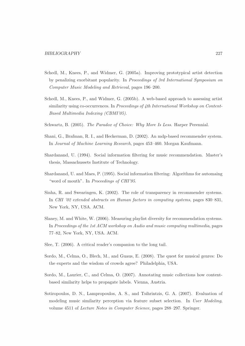
BIBLIOGRAPHY 227
Schedl, M., Knees, P., and Widmer, G. (2005a). Improving prototypical artist detection
by penalizing exorbitant popularity. In Proceedings of 3rd International Symposium on
Computer Music Modeling and Retrieval, pages 196–200.
Schedl, M., Knees, P., and Widmer, G. (2005b). A web-based approach to assessing artist
similarity using co-occurrences. In Proceedings of 4th International Workshop on Content-
Based Multimedia Indexing (CBMI’05).
Schwartz, B. (2005). The Paradox of Choice: Why More Is Less. Harper Perennial.
Shani, G., Brafman, R. I., and Heckerman, D. (2002). An mdp-based recommender system.
In Journal of Machine Learning Research, pages 453–460. Morgan Kaufmann.
Shardanand, U. (1994). Social information filtering for music recommendation. Master’s
thesis, Massachussets Institute of Technology.
Shardanand, U. and Maes, P. (1995). Social information filtering: Algorithms for automaing
“word of mouth”. In Proceedings of CHI’95.
Sinha, R. and Swearingen, K. (2002). The role of transparency in recommender systems.
In CHI ’02 extended abstracts on Human factors in computing systems, pages 830–831,
New York, NY, USA. ACM.
Slaney, M. and White, W. (2006). Measuring playlist diversity for recommendation systems.
In Proceedings of the 1st ACM workshop on Audio and music computing multimedia, pages
77–82, New York, NY, USA. ACM.
Slee, T. (2006). A critical reader’s companion to the long tail.
Sordo, M., Celma, O., Blech, M., and Guaus, E. (2008). The quest for musical genres: Do
the experts and the wisdom of crowds agree? Philadelphia, USA.
Sordo, M., Laurier, C., and Celma, O. (2007). Annotating music collections how content-
based similarity helps to propagate labels. Vienna, Austria.
Sotiropoulos, D. N., Lampropoulos, A. S., and Tsihrintzis, G. A. (2007). Evaluation of
modeling music similarity perception via feature subset selection. In User Modeling,
volume 4511 of Lecture Notes in Computer Science, pages 288–297. Springer.

228 BIBLIOGRAPHY
Soundscan, N. (2006). Year–end music industry report.
Soundscan, N. (2007). State of the industry. National Association of Recording Merchan-
disers.
Swearingen, K. and Sinha, R. (2001). Beyond algorithms: An hci perspective on recom-
mender systems. In ACM SIGIR. Workshop on Recommender Systems, volume Vol. 13,
Numbers 5-6, pages 393–408.
Symeonidis, P., Ruxanda, M., Nanopoulos, A., and Manolopoulos, Y. (2008). Ternary
semantic analysis of social tags for personalized music recommendation. In Proceedings
of 9th International Conference on Music Information Retrieval, Philadelphia, USA.
Takacs, G., Pilaszy, I., Nemeth, B., and Tikk, D. (2008). Investigation of various matrix
factorization methods for large recommender systems. In Proceedings of the 2nd KDD
Workshop on Large Scale Recommender Systems and the Netflix Prize Competition.
Tiemann, M. and Pauws, S. (2007). Towards ensemble learning for hybrid music recommen-
dation. In Proceedings of 8th International Conference on Music Information Retrieval,
Vienna, Austria.
Tintarev, N. and Masthoff, J. (2007). Effective explanations of recommendations: user-
centered design. In Proceedings of the 2007 ACM conference on Recommender systems,
pages 153–156, Minneapolis, MN, USA. ACM.
Tsinaraki, C. and Christodoulakis, S. (2005). Semantic user preference descriptions in
mpeg-7/21.
Tso-Sutter, K. H. L., Marinho, L. B., and Schmidt-Thieme, L. (2008). Tag-aware recom-
mender systems by fusion of collaborative filtering algorithms. In Proceedings of the 2008
ACM symposium on Applied computing, pages 1995–1999, New York, NY, USA. ACM.
Tucker, C. and Zhang, J. (2008). How does popularity information affect choices? theory
and a field experiment. SSRN eLibrary.
Turnbull, D., Barrington, L., and Lanckriet, G. (2008). Five approaches to collecting tags
for music. In Proceedings of the 9th International Conference on Music Information
Retrieval, pages 225–230, Philadelphia, USA.

BIBLIOGRAPHY 229
Tzanetakis, G. (2002). Manipulation, analysis and retrieval systems for audio signals. PhD
thesis.
Uitdenbogerd, A. and van Schnydel, R. (2002). A review of factors affecting music recom-
mender success. In Proceedings of 3rd International Conference on Music Information
Retrieval, Paris, France.
van Gulik, R. and Vignoli, F. (2005). Visual playlist generation on the artist map. In
Proceedings of 6th International Conference on Music Information Retrieval, pages 520–
523, London, UK.
Vembu, S. and Baumann, S. (2004). A self-organizing map based knowledge discovery for
music recommendation systems. In Computer Music Modeling and Retrieval, Esbjerg,
Denmark.
Vignoli, F. and Pauws, S. (2005). A music retrieval system based on user driven simi-
larity and its evaluation. In Proceedings of the 6th International Conference on Music
Information Retrieval, pages 272–279, London, UK.
Vuong, Q. H. (1989). Likelihood ratio tests for model selection and non-nested hypotheses.
Econometrica, 57(2):307–33.
Watts, D. J. and Strogatz, S. H. (1998). Collective dynamics of ’small-world’ networks.
Nature, 393(6684):440–442.
Webb, G. and Kuzmycz, M. (1996). Feature based modelling: A methodology for produc-
ing coherent, consistent, dynamically changing models of agents’ competencies. In User
Modeling and User-Adapted Interaction, pages 117–150.
Weng, L.-T., Xu, Y., Li, Y., and Nayak, R. (2007). Improving recommendation novelty
based on topic taxonomy. In Proceedings of the IEEE/WIC/ACM International Confer-
ences on Web Intelligence and Intelligent Agent Technology, pages 115–118, Washington,
DC, USA. IEEE Computer Society.
Whitman, B. (2003). Semantic rank reduction of music audio. In Proceedings of the 2003
Workshop on Applications of Signal Processing to Audio and Acoustics (WASPAA), pages
135–138.
230 BIBLIOGRAPHY
Whitman, B. and Lawrence, S. (2002). Inferring descriptions and similarity for music
from community metadata. In Proceedings of International Computer Music Conference,
Goteborg, Sweden.
Xu, Y., Zhang, L., and Liu, W. (2006). Cubic analysis of social bookmarking for personalized
recommendation. Frontiers of WWW Research and Development, pages 733–738.
Yang, Y. and Li, J. Z. (2005). Interest-based recommendation in digital library. Journal of
Computer Science, 1(1):40–46.
Yao, Y. Y. (1995). Measuring retrieval effectiveness based on user preference of documents.
J. Am. Soc. Inf. Sci., 46(2):133–145.
Yoshii, K., Goto, M., Komatani, K., Ogata, T., and Okuno, H. G. (2006). Hybrid collab-
orative and content-based music recommendation using probabilistic model with latent
user preferences. In Proceedings of 7th International Conference on Music Information
Retrieval, pages 296–301, Victoria, Canada.
Yoshii, K., Goto, M., Komatani, K., Ogata, T., and Okuno, H. G. (2007). Improving
efficiency and scalability of model-based music recommender system based on incremental
training. In Proceedings of 8th International Conference on Music Information Retrieval,
Vienna, Austria.
Yoshii, K., Goto, M., Komatani, K., Ogata, T., and Okuno, H. G. (2008). An efficient hy-
brid music recommender system using an incrementally trainable probabilistic generative
model. IEEE Transaction on Audio Speech and Language Processing, 16(2):435–447.
Yoshii, K., Goto, M., and Okuno., H. G. (2004). Automatic drum sound description for
real-world music using template adaptation and matching methods. Proceedings of 5th
International Conference on Music Information Retrieval.
Zadel, M. and Fujinaga, I. (2004). Web services for music information retrieval. In Proceed-
ings of 5th International Conference on Music Information Retrieval, Barcelona, Spain.
Zhang, Y., Callan, J., and Minka, T. (2002). Novelty and redundancy detection in adaptive
filtering. In Proceedings of the 25th international ACM SIGIR conference on Research
and development in information retrieval, pages 81–88, New York, NY, USA. ACM.

BIBLIOGRAPHY 231
Ziegler, C.-N., McNee, S. M., Konstan, J. A., and Lausen, G. (2005). Improving recom-
mendation lists through topic diversification. In Proceedings of the 14th international
conference on World Wide Web, pages 22–32, New York, NY, USA. ACM.
Zils, A. and Pachet, F. (2003). Extracting automatically the perceived intensity of music
titles. 6th International Conference on Digital Audio Effects.

232 BIBLIOGRAPHY


