N A S A

-. - . .

C O N T R A C T O R 11 N A S A C R - 2 3 0 R E P O R T 2$ p

DIGITAL ANALYSIS OF LIQUID PROPELLANT SLOSHING IN MOBILE TANKS WITH ROTATIONAL SYMMETRY

bji D. 0. Lomen

Prepared under Contract No. NAS 8-11193 by GENERiQL DYNAMICS/ ASTRONAUTICS

Sail Diego, Calif.

jbr

N A r l O N A L A E R O N A U T I C S A N D SPACE A D M I N I S T R A T I O I N W A S H I N G T O N , D. C . M A Y 1 9 6 5

https://ntrs.nasa.gov/search.jsp?R=19650014214 2020-05-11T00:48:46+00:00Z

SECTION 1

INTRODUCTION

The hydrodynamic forces and moments are derived (in Reference 1) for tanks pos- sessing a longitudinal axis of symmetry. These forces and moments are given in terms of coefficients which depend only on the tank geometry.

This report explains the steps used to obtain these coefficients, given the tank geom- etry, and the procedures used in the program check-out. A description of the routines used in the program is included as well as instructions for use of the program. The output of the digital program gives the spring-mass parameters associated with the system.

The digital routines were developed and programed by Roger Barnes.

f l

1-1

NASA CR-230

DIGITAL ANALYSIS OF LIQUID PROPELLANT SLOSHING

IN MOBILE TANKS WITH ROTATIONAL SYMMETRY

By D. 0. Lomen

Distribution of th i s report is provided in the interest of information exchange. Responsibility for the contents resides in the author o r organization that prepared it.

Prepared under Contract No. NAS 8-11193 by GENERAL DYNAMICS/ASTRONAUTICS

San Diego, Calif.

for

NATIONAL AERONAUTICS AND SPACE ADMINISTRATION

For sale by the Clearinghouse for Federal Scientific and Technical Information Springfield, Virginia 22151 - Price $2.00

Section

TABLE OF CONTENTS

Page

1- 1 1 INTRODUCTION . . . . . . . . . . . . . . . . . . 2- 1

2-1 2-3

2 SYNTHESIS OF EQUATIONS . . . . . . . . . . . . . . 2 . 1 Hydrodynamic Equations . . . . . . . . . . . . . 2 . 2 Synthesis for Digital Equations . . . . . . . . . . .

3-1

3 . 1 Driver Routines . . . . . . . . . . . . . . . . 3-1

3 ROUTINES OF THE COMPUTER PROGRAM. . . . . . . . .

. . . . . . . . . . . . . . . . . . 3-3 3 .3 Bessel Functions . . . . . . . . . . . . . . . . 3-4 3 .2 Integration

4- 1

4- 1 4-5

4 . 3 Setup for a Computer Run . . . . . . . . . . . . . 4-6

4 UTILIZATION OF THE COMPUTER PROGRAM . . . . . . . 4 . 1 Description of Program Input. . . . . . . . . . . . 4 . 2 Description of Program Output . . . . . . . . . . .

5- 1 5 CHECK-OUTOFTHEDIGITALPROGRAM . . . . . . . . . 6- 1 6 REFERENCES. . . . . . . . . . . . . . . . . . .

Appendix

SAMPLE CASE FOR ATLAS TANK . . . . . . . . . . . . A-1

ii i

SECTION 2

SYNTHESIS OF EQUATIONS

2.1 HYDRODYNAMIC EQUATIONS. The equations which describe the sloshing of liquid propellant in a tank consisting of an arbitrary curve rotated about an axis of

I symmetry are derived in Reference 1 and are:

3 F3' = -Ma!

OD .. .. F 2 ' = - M a -ML13 - M C b y n n n 5

n= 1 2

n 3 n n ' i ' - M C y a b 5 + [L(bn-hn) I OD

= ML Q + n= 1 T1 1 2 51

(2.4)

where

I 7 is the surface wave height

I F and F2I are forces in the x 3 and x 2 directions (see Figure 2-1) 3

I T1 I is the moment about the x axis 1

@ (r , z) are eigenfunctions n

a ( t ) is given by the solution of (2.5).

(2.5) n K .. h(t) +a - 6 (t) = -K b Q! (t) - Kn [Lib, - L - hn)] (t) 3 L n n n 2

2 LW n

3 TheK =- are nondimensional frequencies, L is the distance from the center of

gravity of the liquid to the undistrubed free surface, and L1 is the distance from the

n Q !

2-1

J

center of gravity of the liquid to an arbitrary point along an extension of the line AC (see Figure 2-1).

z

*1

Figure 2-1. Tank of Arbitrary Shape

The component of acceleration along the x (x ) axis is denoted by a @ ). The con- stants in ( 2 . 3 ) , (2 .4 ) , and (2 .5) are given %y 2 3 2

B

yn = r [Gn ( r , L ) I 2 d r

C

B 2

bn = r Qn ( r , L) d r

C

B h = 2n f z ran ( r , z ) dz n VYnKn

A

2-2

l and

2 2 I1 1 ' = pJ (x2 + x 3 ) dV - 4p f x t d V + 2pL2 f x3v2$ldS

uv uv us

2 + L 1 M

M is the total mass and V the total volume of the liquid.

n r 1 W

r + A I (p r) c o s p n (z + d ) , p n = h 0 n l n n=l

where A is to be determined from the equation n

(2.10)

d F m

A. +c Anpn F(z)) cos p (z + d) +-I (p F(z)) sin p n (z + d) n dz 1 n n=l

(2.11)

To find an approximation for G1, truncate the series to include N + 1 terms. Evaluate (2.11) at N + 1 points (zi) on the boundary to obtain the following set of linear equations for the determination of the pfi , i .e.

d F dz +- (zi) I1 (pnF(zi)) sin p n i (z. + d) i = 1 , 2 , . . . , N + 1 (2.12)

I where r = F(z) is the equation of the boundary AB,

2.2 SYNTHESIS FOR DIGITAL SOLUTION. determination of the eigenfunctions, @ and eigenvalues, K is

The boundary value problem for the

n ' n '

a+ o a2a n

2

a2Q n l n n -+- - - -+- - - 0

br r az 2 r br (2.13)

2-3

a* n

av -- - 0 (on AB)

(on BC)

I It has been shown (Reference 2) that the Kn/L may be found by minimizing the quotient

L

(2.14)

(2 .15)

(2.16)

I UFS

To reduce the magnitude of the variables in integration, make the problem described by (2.13) through (2.16) nondimensional by letting

R = r / a

@ (Ra, Za) = @ (R ,Z)

a = the distance from B to the z-axis.

If the free surface of the liquid does not intersect the center line of the tank, A and C coincide. In this situation, let ' the distance from the z-axis to point C be designated by R1, and define c = R /a. 1

I Thus

a20 1 3~ a20 2 R aR R2 az 2

-+- - - - + - = o bR

(2.17)

(on AB)

(on BC)

2 -4

(2.18)

(2 .19)

C

where the integrations a re over nondimensional limits (see Figure 2-2).

Z

(2.20)

Figure 2-2. Nondimensiond Geometry

Following the pattern of Reference 2 , let @ be expressed as a linear combination of the eigenfunctions for a shallow tank and eigenfunctions for a deep cylindrical tank, and use a Rayleigh-Ritz technique. Let

K a L

=-

and substitute

(2.21)

(2.22)

n= 1

2-5

into (2.20); differentiate with respect to cm, and set the result equal to zero to obtain

n= 1

where

a mn = /

UA

B

* * * * * * -- + +-n

a@ 30 a@ aR 3R 2 az az

m @ @

R

n m n m

* * b = @ (R, L/a )# (R, L/a)RdR mn m n

(2.23)

RdRdZ (2.24)

(2.25)

C *

The set of functions @ (R, Z) are chosen, for reasons mentioned previously, as n

R2n- 1 n =1, 2 , . . . , M<N*

j (z-L/a) n Jl(jnR) e , n = M + l , . . . , N*

g* (R, Z) = (2.26)

where

(2.27)

and the first root of (2.27) is called j M + 1 '

The b are calculated as mn

2n+2m 1 2m-1 2n-1 1 - €

b = J R R RdR = , m , n s M 2n + 2m mn (2.28)

2-6

I where

(2.29)

2 2 2 2 2 2 (j, - 1) J1 (x) -[jncJl' (jnc)l - (jn c - 1) J1 (jnc)

, n > M (2.30) 2 b = nn

2jn

1 b =J R2m J1 (jnR) dR, m 5 M < n

mn c

- 4m (m - 1) b (m-l)n

(2.31)

(2.32)

Substitute the value of c $ ~ * from (2.26) into (2.24) to obtain the following expressions for amn. Thus, by Green's theorem

RdRdZ, n , m I M 1 2n+2m-4 a = j [ ((2m - 1) (2n - 1) + 11 R mn

UA

R2n+2m-3 ZdR

C

(see Reference 3 , P. 239)

(2.33)

2 -7

In a similar manner

jn ( z - L/a) 2m-2 d -J (j R ) e

mn dR 1 n

RdRdZ, m I M < n jn( Z- L/a) + R2m-3

J1 UnR) e

jn( Z - L/a) j J '(j R) + R2m-2J (j R)] e dR (2.34)

- 2m-1 - -L$ jn [,,m - 1) R n l n I n

C

and

d -1 ran R) + R J1 (jnR) J1 (jmR)

UA j (Z-L/a) j n (Z-L/a)

+ R j j J (j R) Jl(jmR) e.n e dRdZ, n, m > M 1 n m 1 n

-1 R jnjm J1 'a$) J1 ' ( j R) + R J1 ( j n R) J l m (j R) m

Once the b and am a r e etermined, the eigenvalue problem can be solved yielding 4 and the 11211 correspon&ng cn R . I th The k mode is given by

(2. 36) n =1

2 -8

I Its dimensional form is

(2.37)

It is this value which must be used in the evaluation of (2.6), (2.7) and (2.8). The K a r e given by I n

L n , a n

K =-A

Thus

B b ="/ r 2 Cp ( r , L) d r

n VYn n I C

Similarly

B 2 N*

k=l c - --!!- C c:j r $* (r/a, L/a) dr

VY

3 N*

n k=l

na n w

1 2 3 N*

- - E x cknJR @ * (R, L/a) dR =-c c b k lk

€ "n k=l

n n 2N* N*

nLa m=----CC kli=l Ck c i bki

Where ~

B h * = / ZRXndZ n M n

A

B j p -L/a) h * =$ ZR J1 UnR) e dZ M < n s N* n

A

(2.38)

(2.39)

(2.40)

(2.41)

(2.42)

(2.43)

2-9

11 ’ Finally consider the evaluation of I

+ x 2, dV = p./ (r 2 + 22 2 ) rdrdz 3

uv UA

5 - 4 p s x3 2 dV =- ypm $ RZ’dR

3

(2.44)

(2.45)

uv - C

m

SpL21 x3v2 lijdS = 2pnL A I ( p r )cosp (z + d) dz (2.46) n 1 n l n

us A

2-10

SECTION 3

ROUTINES OF THE COMPUTER PROGRAM

The routines of the computer program are coded in the FORTRAN IV language, with the exception of par ts of a SHARE simultaneous equation routine (SOLVE) and a SHARE eigenvalue routine (RWEGBF).

3 . 1 DRIVER ROUTINES, eigenvalues of (2.23). Elements of the amn and bmn matrices a re computed for ten eigenfunctions, of which the first five a re polynomials. The integration to evaluate the am elements is described in Section 3.2. The Bessel functions needed for the elements of both matrices a r e computed by a routine described in Section 3.3. The resultant eigenvalues, and their eigenvectors, are found by the Jacobi method using the routine RWEG2F.

The boundary value problem requires solution of the

Routine RWEG2F solves an eigenvalue problem of the form:

1.1 [.I ="PI IXI where the B matrix must be positive definite. .Now it was found that the b,, matrix

I though the amn matrix did, Therefore, jetting is rewritten:

where

I 1 x =y The A' eigenvalues are found and then inverted to give the desired eigenvalues of (2.23). Each corresponding eigenvector is normalized by its largest element.

(3.3)

For each mode of oscillation entered as input data, the nondimensional frequency (K,) i s computed by (2.38). Force and moment coefficients (Yn, bn, and h ) are computed using (2.39) through (2.43), where the hn* factor of $ employs a Bessel function, Section 3.3, and integration, Section 3.2. The above coefficients are then combined as in (2.47) through (2.52) to yield the spring-mass parameters (mn, An, %*/a3, m A 0' 0'

Therefore, L1 = d in the expressions for an, io, and Io. The Ill ' t e rm of I is found by (2.9). The first two terms of I Section 3.2.

' n

and Io). The center of rotation is assumed to be at the bottom of the tank.

I Q are found by the integration described rn 11

3-1

Calculation of the third term of Ill ' requires the solution of a set of simultaneous linear equations, yielding the coefficients, A Equation (2.12) is evaluated at selec- ted points on the rigid tank wall below the undisturbed free surface. The total number of points selected, n , must be such that:

n.'

where R surface.

is the maximum radius of the rigid tank wall below the undisturbed free max

(2) n 5 50

Restriction (1) is necessary to prevent the modified Bessel function in the equation from exceeding about1016, making other te rms of the equations completely insignifi- cant. Restriction (2) is set by program core storage limitations. In general, points selected by the program will be end points of segments with equally spaced points be- tween, point B, and point C (if € # 0) on Figure 2-2. The resultant set of simultane- ous linear equations is solved by the routine SOLVE. Integration, again as in Section 3 . 2 , is then done on (2.46) with the coefficients, A . n

3 -2

3.2 INTEGRATION. Integration is performed using Gauss's Quadrature Formula:

/b f(u) du = (b-a) /I2 @ (t) dt = S1 @ (t,) + S2 @ (t,) + . . . a - 1/2

+ s @ ( t ) n n (3 4)

where n is taken to be 16 and u = (b-a) t + a.

The sum in (3.4) is taken by adding the smallest term to the next largest and so on, to obtain the most accuracy when f(u) is increasing from a to b.

Two integration routines were written:

1. INTGl - - for line integrals of the form

B f (2) dz J

A

The line integral is taken in a counterclockwise direction along each segment of the rigid tank wall from A to B. (See Figure 2-1. )

B 22 23 zn f ( z ) dz = f (z) dz + f (z) dz + - . . +/f (z) dz J J J

A 2 1 z2 Zn-1

(3.5)

where

zl, 22, . . . , z ~ - ~ a r e the z-coordinate of end points of segments entered as input; and zn is the z-coordinate at the outer radius of the undisturbed free surface.

I 2. INTGB -- for line integrals of the form

C The line integral is taken in a counterclockwise direction around the fluid of the c ross section of the tank as in Figure 2-1.

3 -3

B C

C A B

With r-coordinate limits of integration for each segment of the rigid tank wall from A to B and the undisturbed free surface, (3.6) is rewritten

f C

j: a

d r

r3 d r +Jf (r)

r2

(3.7)

where

rl, r g , r3, . . . , rn-l are the r-coordinate of end points of segments entered as input; a is the outer radius; and R1 is the inner radius of the undisturbed free surface.

Equation (3.4) is then applied to each term of (3.5) and (3.7).

3.3 BESSEL FUNCTIONS. Two types of Bessel Functions are computed: the first kind of order one (J1 (x) ) and its derivative (J; (x) ), and the modified of order one (Il(x) ) and its derivative (Ii (x) ).

The BESSEL routine computes, in double precision, Jl(x) and J;(x) by the ascending series:

1 = 1 k! (k+l)! k=l

(3.9)

k=l kl

3 -4

Each term of the above series is found by multiplying the previous te rm by the appro- priate factor:

(-1) 2 for J- (x) and the second part of J ‘ (x)

1 (3.10)

for the first part of J ’ (x) (3.11) 1

(-1) (“)2 2

9 Since 0 * x * 14.863588 in the program, the above technique is sufficiently accurate for the range of x.

Routine RMODBS computes, in double precision, the I (x) and I ‘ (x) by polynomial approximations, with t = x/3.75. 1 1

For -3.75 5 x s 3 . 7 5 :

2 I1 (x) = x 1/2 + 0.87890594 t

4 6 + 0.51498869 t + 0.15084934 t 8 10 + 0.02658733 t + 0.00301532 t

+ 0.00032411 t12 1

I I1 (XI I1 (x) = Io (x) --

X

where 2 I (x) = 1 + 3.5156229 t

4 6 +3.0899424 t + 1.2067492 t 8 10

+O. 2659732 t + 0.0360768 t 12 +0.0045813 t

0

(3.12)

(3.13)

(3.14)

3-5

For 3.75 * x C m :

I1 (x) = x-1’2ex [O. 39894228 - 0.03988024 t-’

- 0.00362018 t-2 + 0.00163801 t-3

- 0.01031555 t-4 + 0.02282967 t-5

- 0.02895312 t-6 + 0.01787654 t-7

- 0.00420059 t-8

T I

I1 (x) I I (x) = I (x) - 1 0 X

where

-1/2 x I (x) = x e 10.39894228 + 0.01328592 t-’ 0

+ 0,00225319 t-2 - 0.00157565 t-3 + 0.00916281 t-4

- 0.02057706 tm5 + 0.02635537 t-6 - 0.01647633 t-7

+ 0.00392377 t-8]

(3.15)

(3.16)

(3.17)

3 -6

SECTION 4

UTILIZATION OF COMPUTER PROGRAM

4.1 DESCRIPTION OF PROGRAM INPUT. Three sets of numerical data are re- quired as input for a computer run. Sections 4.1.1 through 4.1.3 describe this data, which is subject to limitations that are outlined in Section 4.1.4. All numbers are entered on 80-column input forms. Each digit of a number or a decimal point (if needed) occupies one column. Unless otherwise specified in the follow mg sections, a number must be entered with a decimal point. The decimal point may be anywhere within the columns allocated for that number on the input form.

A number that must not have a decimal point must be right-adjusted. That i s , all digits must occupy the right-most columns of those allocated for the number; there may be no blank columns between the number and the last column, inclusive.

Extremely large or small numbers may be entered a s a coefficient times ten to a power:

I

I Here a decimal point must be in the coefficient, and the last digit of the exponent must occupy the last column of those allocated for the number.

All coordinates required as input must be from a system in which the r-coordinate of the centerline is zero, and the z-coordinate increases upward.

4-1

4.1.1 quired to set up the problem for the computer.

Problem Input. The first line of the input form contains that set of data re-

Columns Data - 1 through 10 Enter the number of segments that describe the rigid tank

wall. The number must be right-adjusted, without a dec- imal point,

11 through 20 Enter the number of modes of oscillation desired. The number must be right-adjusted, without a decimal point.

21 through 30 Enter the liquid density (in pounds per cubic foot).

31 through 40 Enter the r-coordinate (in inches) of the beginning of the segments that describe the tank.

41 through 50 Enter the z-coordinate (in inches) of the beginning of the segments that describe the tank.

4.1.2 of the data below is required for each segment that describes the rigid tank wall. Seg- ments must be ordered in a continuous, counterclockwise path around the tank. The number of these lines of input must equal the number entered in columns 1 through 10 of the first line (i.e. number of segments).

Tank Geometry Input. Beginning with the second line of the input form, a line

Data - Columns

1 through 10 Enter the r-coordinate (in inches) of the end of the partic- ular segment, having proceeded along it in a counterclock- wise direction around the tank.

11 through 20 Enter the z-coordinate (in inches) of the end of the particu- lar segment, having proceeded along it in a counterclock- wise direction around the tank.

21 through 30 Leave blank for a straight line segment; otherwise, enter as follows, depending on the type of segment:

Elliptical. Enter the r-coordinate (in inches) of the center of the ellipse.

Circular. Enter the r-coordinate (in inches) of the center of the circle.

4- 2

I Columns Data - 21 through 30 (Contd) of the parabola.

Parabolic. Enter the r-coordinate (in inches) of the vertex

31 through 40 Leave blank for a straight line segment; otherwise, enter I as follows, depending on the type of segment:

Elliptical. Enter the z-coordinate (in inches) of the center of the ellipse.

Circular. Enter the z-coordinate (in inches) of the center of the circle.

Parabolic. Enter the z-coordinate (in inches) of the vertex of the parabola.

41 through 50 Leave blank for a straight line segment; otherwise enter, depending on the type of the segment, a s fol- lows:

Elliptical. Enter the semimajor axis (in inches) of the ellipse.

Circular. Enter the radius (in inches) of the circle.

Parabolic. Enter the directrix (in inches) of the parabola.

51 through 60 Leave blank for a parabolic or straight line segment; otherwise enter, depending on the type of the segment, as follows:

Elliptical. Enter the semiminor axis (in inches) of the ellipse.

Circular. Enter the radius (in inches) of the circle.

61 through 70 Leave blank for a circular o r straight line segment; enter the amount of counterclockwise rotation from the norm (see below) of the ellipse if the segment is elliptical, or of the parabola if the segment is parabolic. It may be left blank for an angle of zero degrees.

4- 3

Normal Position of an Ellipse

2

SEMIMINOR A X I S

A CENTER’ LSEMIMAJOR AXIS

Normal Position of a Parabola

4.1.3 Case Input. number of cases may be run.

Each case to be run requires a line of input as listed below. Any

Data - 1 through 10 Enter the z-coordinate (in inches) of the liquid level in the tank.

4.1.4 Limitations on Input. data.

The following restrictions must be applied to the input

1. There can be no more than 50 segments.

2. Each segment must be such that for a given radius, there is only a single value of the height.

4 -4

I i . e . A toroid must be described by four segments of the same circle:

I Z

3 . The liquid level must not indicate a completely full tank.

4. There can be no more than ten modes of oscillation.

5 . Do not enter the centerline segment unless it i s , in reality, a part of the rigid tank wall.

4.2 DESCRIPTION OF PROGRAM OUTPUT. sists of the following:

Printed output on a computer run con-

1. Tank Geometry. A complete definition of all segments entered a s input.

And for each liquid level case:

2. Liquid Level. The z-coordinate (in inches) of the undisturbed free surface in the tank.

3. Mass of Liquid. The mass (in pounds) of the liquid contained in the tank.

4 . Center of Gravity. The z-coordinate (in inches) of the center of gravity of the liquid.

I l l ' and its four terms (in lb-in. ).

Eigenvalue Statistics. These, for each mode requested, a r e the eigenvalue and the eigenvector and its normalizing factor,

2 5 .

6 .

7 . For each mode requested, the coefficients (Kn, Yn, bn, and h ) of the force and moment equations. n

4-5

8, For ach mod requested, the following parame,xs for the spring-mass analogy:

m (in pounds) n

(in inches) n

Kn*/a3 (in lb/in. )

9. Also, the following spring-mass parameters:

m (in pounds) 0

(in inches)

2 I (in lb-in. )

0

0

These parameters are a summation for all modes of oscillation entered as input data, and printed out in item 8 above. Therefore, if a one-mode analysis is to be used, only one mode should be entered as input data.

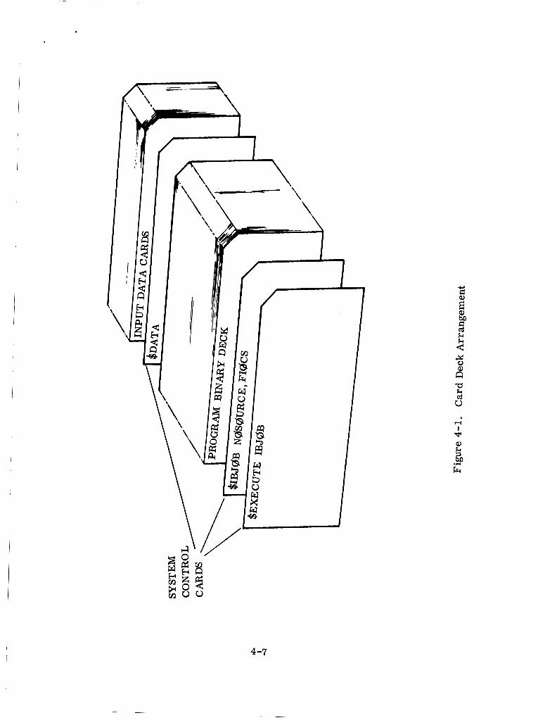
4.3 containing system control cards , the program binary deck, and input data cards. The input data is punched on cards from the 80-column coding form described in Section 4.1. Arrangement of the deck will be as shown in Figure 4-1.

SETUP FOR A COMPUTER RUN. A run on the computer requires a card deck

The program is designed to be run under the IBSYS monitor system. For the IBM 7094 computer, execution time estimates should be based on about 10 millihours per segment per liquid level case.

4 -6

4-7

SECTION 5

CHECK-OUT OF THE DIGITAL PROGRAM

The output of the computer program was checked against the experimental and (if possible) theoretical data available for tanks comprised of spheres, toroids, oblate spheroids, right circular cylinders, and concentric right circular cylinders.

The volume and center of gravity of the fluid as well as the first two integrals in (2.9) may be easily checked out by hand-calculation for any tank configuration. The nondimensional frequencies, I(n, may be checked for any tank configuration that has analytical o r experimental results available. The operations involved in finding these five quantities constitute the major portion of the program. The rest of the program simply manipulates these terms. Thus if these five quantities are calculated properly and the multiplications and additions required for the evaluation of the rest of the terms are checked out for a particular case, one is assured that the entire pro- &am is working properly. The only term which must be checked out in a different manner is the third te rm of (2.9). The boundary value problem for 9 (see Reference 1, Equations 3.10 and 3.11) may be solved explicitly for specialized cases only. The shapes checked out here were for a right circular cylinder at various liquid levels. For a cylinder of radius 60 inches and liquid level 50 inches the calculated value was 1.36 X lo8 , the computer obtained 1.3779 X lo8. For a liquid level of 240 inches, note the comparison of I, on page 5-6. Since 9 is approximated using Bessel func- tions, the routine is not very accurate for elliptical or spherical tanks. However if the tank is "close to cylindrical" in shape, the output is good. That is, for the two Atlas tanks the routine calculates Io properly. A rough check on this term for any tank shape is to compare the four terms comprising I l l ' , If the third term is of different magnitude than the other three, i t is not usable, The approximation then used is that Il l ' equals the sum of the first and fourth terms.

1

The routines for a parabolic section were checked by using a cylindrical tank of radius 60 inches with a parabolic bottom. The Darabola had a directrix of 5000 and thus approximated a straight line. The difference between the output for this shaoe and the output for a cylinder with a flat bottom were different only in the third signi- ficant digit.

5- 1

Figure 5-1 shows the comparison of the lowest three frequencies of a spherical tank (radius of 60 inches) with a graph f rom Reference 3. In this figure, where R is the radius of the sphere and h the liquid height, note that the lowest frequencies fall on the dark line while the next two sets of frequencies appear at times to be closer to the experimental rather than the theoretical results.

The check for the lowest frequencies for an oblate spheroidal tank is given in Figure 5-2. The tank used in this program had a semimajor axis of 26.26 and a semiminor axis of 13.13 and was compared with the results in Reference 4. Note that only the lowest mode frequencies are shown here. The frequencies for the second mode were 50 percent greater than test data. This is explained by the statement of Reference 2 -- that the accuracy depends on the choice of eigenfunctions and the experience Rayleigh (Reference 5) had in approximating an ellipse using Bessel functions.

The comparison of frequencies for a toroidal tank, with results from Reference 6, is shown in Figure 5-3. Note the good agreement for the two lowest modes.

The frequencies for a ring tank, inner radius 10 inches and outer radius 60 inches, were checked against the analytical solution for a liquid height of 50 inches. (Use must be made of the tables in Reference 7 . ) The results appear in the table below.

ANALYTICAL COMPUTER

0.6618 0.6616 K1

Kg

K4

2 . 0 9 1

3.481 3.496

4.956 4 .933

Kg 2.090

The program's entire output may also be checked out against the analytical solutions (Reference 1, p. 3-8) for a right circular cylindrical tank. Because of a difference in normalization in the computer program and the analytical work, the parameters

bn/hn, and ynbnk which appear in the spring-mass parameters are independent of the normalization. Thus, if the spring-mass parameters check out (using results of Reference 1, p. 3-8) the yn, bn, hn are being calculated properly. If desired, how- ever, these combinations could be checked out by themselves. The comparison of parameters is given in the following table for a tank of radius 60 inches and height of 300 inches, filled to a depth of 240 inches with a liquid having a density of 1 ,

y,, b,, and hn may not be directly compared. However the combinations ynbn 2 ,

5-2

I c. g.

K1

K2

~ ~ Kg

y1

bl

hl

I

l a 1

m 1

K,*/Cr3

, m I 0

a

M

l

0

0 I

ANALYTICAL RESULTS

120.

3.682

10.663

17.073 4

3.729 X 10

9.0965 X 10 -4

-4 13.259 X 10

174.91 6

0.30837 X 10

3 9.4628 X 10

6 2.4059 X 10

112.96 6

2.7143 X 10

0.14973 X

COMPUTER OUTPUT

120,

3.6823

10.663

17.073

0.5969

0.71901

1.0486

175.0 6

0.30841 X 10

3

6 9.4639 X 10

2.4059 X 10

112.95 6

2.7143 X 10

0.15081 X 10 11

5-3

4.0

LIQUID-DEPTH RATIO, h/2R

I I 1 1 I 0 WATER

[I A MERCURY 8

0 DATA FROM REF,

0

Figure 5-1. Theoretical and Experimental Values of Natural Frequency Parameters for the First Three Modes

5-4

n J,

4*01-

FIR

a, in 3.10 6.43 13.13

0.4 -

1 I I 1 1 0.6 ' 0.8 1.0 0.2 0.4 b

0. 0

4.0-

3.6 -

3.2 -

2.8 -

2.4 - FIRST

2.0 -

1.2 - a, in 3.10

0.8 - 6.43 8 13.13 0

0.4 -

1 I I 1 1 0.6 ' 0.8 1.0 0.2 0.4 b

0. 0

FULLNESS RATIO, h/2a

ST

e 8 0

MODE

Figure 5-2. Variation of Frequency Parameter

Transverse Orientation; b/a = 0.50 with Fullness Ratio for Liquid in

5-5

3.2

2.9

2.4

I 3 PI 2.0 2

R 1 . 6 w ;>

E

1 . 2 Fr

0 . 8

0.4

0

-23.8

- -2r

FIRST BB 1111

0.5 1 .0 h/2r

Figure 5-3. Variation of Liquid Natural Frequency with Fullness Ratio for a Horizontal Toroidal Tank; r = 5.9

5-6

1.

2 .

3 .

4.

5 .

6 .

7.

SECTION 6

REFERENCES

D. 0. Lomen, Liquid Propellant Sloshing in hdbile Tanks of Arbitrary Shape, General Dynamics/Astronautics Report GD I A-DDE64-06 1 , San Diego, 1964.

H. R. Lawrence, C. J. Wang, and R . B. Reddy, "Variational Solution of Fuel Sloshing Modes, ' I Jet Propulsion Vol. 28 No. 11, November 1958, pp. 729-736.

A. J. Stofan and A. A. Armstead, Analytical and Experimental Investigations of Forces and Frequencies Resulting from Liquid Sloshing in a Spherical Tank, NASA TN D-1281, Cleveland, 1962.

H. W. Leonard and W. C. Walton, J r . , An Investigation of the Natural Fre- quencies and Mode Shapes of Liquids in Oblate Spheroidal Tanks, NASA TN D-904, Langley Field, 1961.

Rayleigh, Theory of Sound.

J. L. McCarty, H. W. Leonard, and W. C. Walton, J r . , Experimental InveSti- gation of the Natural Frequencies of Liquids in Toroidal Tanks, NASA TN D-531, Langley Field, 1960.

H. F. Bauer , Theorv of the Fluid Oscillations in a Circular Cvlindrical Ring " - Tank Partially Filled with Liquid, NASA TN D-557, Huntsville, 1960.

6-1

APPENDIX

SAMPLE CASE

FOR

ATLAS TANK

A- 1

A-2

m w I U

$5 > W

m o w . w o o

m~

c a C . D O U l

N

V I m o w w z I I U

VI u u

c I VI o o u K w o m c 9 - Y V a rr a I I I I I

VIVI V

x x H

U

D O C 7 2 4 4 - L L K I I W

u, tfZ ? ? E I

0

I-

a a ~a

- . I t - I 5 2 w w w VIVIU

a c

U I I I l l 1 IOI IIII I I H I l l 1 1 1 1 1

K N U N U N d N dN E N (LN

mVI m w VIV) wlm W V I m v , VIm

0 0 00 00 00 0 0 00 n 0 0 0 0 0 00 00 00

M o m 00 0 9 9 9 91- o c o m U -Y Q 9 u m-Y m u a * 9-

= 0 . . . . . . . . . . . . . .

I O 1 H I 1 I l l 1 I O I 1 1 1 1 I l l 1 1 1 1 1

U N (LN a~ U N (LN (LN M N

W 5. > c

‘y

t c- I u - a X c v)

W z -I I

c I cl)

d

I

a c wl

W z 2 I

c X u I a U c v)

w z 2 I

W z I

-1

cc c VI

a c VI

A-3

.

& o o - o u 0 - N m m & 0 0000000000 0

m c I I I I I I e 0 v w w w w w w w w w w v

w cuotnolnff~Ii(cJI w w z s m o e e u P P m f f z m Z C O O Q e - U m ' m v ) Z - w m e o u + + c c N m w 3 E m W " U " N N " V V V . . . . . . . . . . I ,-4 w 0000000000 w

l l I I

- d 0 4 0 O N O N l \ ( m 0000000000

e - 0 r . 0 0 N - O N N

I I I I I I I I u w w w w w w w w w w

Z P m O S - N m N m P W Q N O I C - Y O ' U ~ O V I c) ~ ~ - D ~ N - N N N

w 0000000000 1 1 I

2 0000000000

- . . . . . . . . . . O

9 0

N 0

W

d

0 W U In m U c

-44 0 0 0 -vl-

0 0 0 . . .

0 I

0 I1 I1

W

e o U I - m u . u 0 I '3

z

p a

m a

r 0 I- U 4 U

e . . 000 N N N o o c

- m ~ 000 I l l

. . . 000 z

L L 0

a

a

-I

I (L W z

a LuLuLu 9 - N -0 . r c o n * Q N m e -

000 . . . . T m N

000 0: 0 c w w w

s m m 4 c 6. U W

w z w w Q 0 u -

VI W V ) w m o s = Z V & Y Z U 0 - c

m w a m 0 : :

V W 1 z W W W I

x w z Lu 0

W -

z I:

0-- 000

z Y

W 0 O x

. . . 000

c VI w m w - ( L o

w U r n

x w X I n

3 m v w P

Z d - d C . 4 9 m

3

4

0 4

0

Iy

d

0 m m

0

I1

w m c N (P 4-

0

VI Q W c w r a a a &

W 0 0 S 0 ,

> 0 0 0

I1 VI c z 0

U

LL U W 0 V

I

I

Ln VI 4 S

I 0 z (L

Y)

I

a

Lu 3 -I

> z W 0

W

a

-

A-4

. 1

11 11 I t

000 I d -

NASA-Langley, 1965 CR-230 A-5