National Health and Nutrition Examination Survey: Calif ... · Classification: LCC RA409 | NLM W2 A...

National Health and Nutrition Examination Survey: California and Los Angeles County, Estimation Methods and Analytic Considerations, 1999–2006 and 2007–2014

Vita

l and

Hea

lth S

tatis

tics

Serie

s 2,

Num

ber

173

M

ay 2

017

Copyright information

All material appearing in this report is in the public domain and may be reproduced or copied without permission; citation as to source, however, is appreciated.

Suggested citation

Parker JD, Kruszon-Moran D, Mohadjer LK, et al. National Health and Nutrition Examination Survey: California and Los Angeles County, estimation methods and analytic considerations, 1999–2006 and 2007–2014. National Center for Health Statistics. Vital Health Stat 2(173). 2017.

Library of Congress Cataloging-in-Publication Data

Names: National Center for Health Statistics (U.S.), issuing body.Title: National Health and Nutrition Examination Survey. California and Los

Angeles County, estimation methods and analytic considerations : 1999-2006 and 2007-2014.

Other titles: California and Los Angeles County, estimation methods and analytic considerations : 1999-2006 and 2007-2014 | Vital and health statistics. Series 2, Data evaluation and methods research ; no. 173. | DHHS publication ; no. 2017-1373.

Description: Hyattsville, Maryland : U.S. Department of Health and Human Services, Centers for Disease Control and Prevention, National Center for Health Statistics, May 2017. | Series: Vital and health statistics, series 2, data evaluation and methods research ; number 173 | Series: DHHS publication ; number 2017-1373 | Includes bibliographical references.

Identifiers: LCCN 2017017756 | ISBN 084060677XSubjects: | MESH: National Health and Nutrition Examination Survey (U.S.) |

Health Surveys | Nutrition Surveys | Data Collection--methods | Sampling Studies | California

Classification: LCC RA409 | NLM W2 A N148vb no. 173 2017 | DDC 362.1072/7--dc23

LC record available at https://lccn.loc.gov/2017017756

For sale by the U.S. Government Printing Office Superintendent of Documents Mail Stop: SSOP Washington, DC 20402–9328 Printed on acid-free paper.

Vital and Health Statistics Series 2, Number 173

National Health and Nutrition Examination Survey: California and Los Angeles County, Estimation Methods and Analytic Considerations, 1999–2006 and 2007–2014

Data Evaluation and Methods Research

U.S. DEPARTMENT OF HEALTH AND HUMAN SERVICES Centers for Disease Control and Prevention National Center for Health Statistics

Hyattsville, Maryland May 2017 DHHS Publication No. 2017–1373

National Center for Health Statistics Charles J. Rothwell, M.S., M.B.A., Director Jennifer H. Madans, Ph.D., Associate Director for Science

Division of Health and Nutrition Examination Surveys Kathryn S. Porter, M.D., M.S., Director Ryne Paulose-Ram, Ph.D., Associate Director for Science

iii

Contents

Acknowledgments iv

Abstract 1

Introduction 1

Sample Weights and Variance Estimation for California and Los Angeles County 2National Sample Designs 2California 3Los Angeles County 3

California and Los Angeles County NHANES Data Files and Characteristics 5Demographics Files 5Sample Weights 5Demographic Characteristics 5NHANES 1999–2006 California, Los Angeles County, and U S Samples 6NHANES 2007–2014 California, Los Angeles County, and U S Samples 8Analytic Issues 8Data Access 10

Summary 10

References 10

Appendix Background: California Sample Weights, 1999–2006 12

Text TablesA Selected features of California National Health and Nutrition Examination Survey, 1999–2006 and 2007–2014 4B Selected features of Los Angeles County National Health and Nutrition Examination Survey,

1999–2006 and 2007–2014 4C Distribution of examination sample weights, among adults aged 20 and over: National Health and

Nutrition Examination Survey, 1999–2006 and 2007–2014 5D Sample sizes and weighted percent distributions of interviewed and examined adults and children:

United States, California, and Los Angeles County National Health and Nutrition Examination Survey, 1999–2006 7E Sample sizes and weighted percent distributions of interviewed and examined adults and children:

United States, California, and Los Angeles County National Health and Nutrition Examination Survey, 2007–2014 9

Appendix TableControl totals for noninstitutionalized civilian population, by domain: California National Health and Nutrition Examination Survey, 1999–2006 16

iv

Acknowledgments

The authors of this report gratefully acknowledge the assistance of Irene Atta, Michele Chiappa, and Jennifer Rammon in the preparation of this report.

Page 1

Introduction

The National Health and Nutrition Examination Survey (NHANES) (1), conducted by the National Center for Health Statistics (NCHS), is a cross-sectional survey of the civilian noninstitutionalized resident population of the United States. NHANES is unique in that it combines a personal interview with a health examination that includes a collection of biological specimens. A nationally representative sample of persons residing in all 50 states and the District of Columbia is selected annually through a complex, multistage, stratified, clustered design that includes approximately 3,100 U.S. counties.

California is the most populous among the U.S. states, and Los Angeles County, California, is the most populous county in the United States (2). In 2010, more than 35 million people, or about 12% of the U.S. population, resided in California, and nearly 10 million people lived in Los Angeles County (2). Furthermore, California and Los Angeles County comprise some of the most diverse populations in the world (3,4). Obtaining subnational estimates on California and Los Angeles County from NHANES data may provide health information unavailable elsewhere.

In 2010, a Los Angeles County data file was created for the combined NHANES 1999–2004 data, and it was made publicly available through the NCHS Research Data Center (RDC) (5). Results from the Los Angeles County NHANES 1999–2004 indicated that the prevalence of selected health conditions was similar for adults in Los Angeles County compared with adults in the United States. The prevalence of obesity, however, was lower in Los Angeles County than in the United States (6). Another study using these data found that the prevalence of antibodies to vaccine-preventable diseases, such as measles, mumps, rubella, and varicella, were similar in Los Angeles County and the United States. Antibody to hepatitis A, cytomegalovirus, and Toxoplasma gondii was higher in Los Angeles County than in the United States (7).

NCHS expanded on this earlier work by creating the California and Los Angeles County NHANES 1999–2006 and 2007–2014 data files (8–11). As with the 1999–2004 Los Angeles County files, methods for the updated 1999–2006 and 2007–2014 California and Los Angeles County data files included combining survey cycles and reweighting the 8-year files to match known California and Los Angeles County population totals. Because Los Angeles County

National Health and Nutrition Examination Survey: California and Los Angeles County, Estimation Methods and Analytic Considerations, 1999–2006 and 2007–2014by Jennifer D. Parker, Ph.D., and Deanna Kruszon-Moran, M.S., National Center for Health Statistics; Leyla K. Mohadjer, Ph.D., Sylvia M. Dohrmann, M.S., Wendy Van de Kerckhove, M.S., and Jason Clark, M.S., Westat; and Vicki L. Burt, Sc.M., R.N., National Center for Health Statistics

Background California is the most populated

state and Los Angeles County is the most populated county in the United States. National Health and Nutrition Examination Survey (NHANES) sample weights and variance units were developed for these places to obtain subnational estimates.

Objective This report describes the California

and Los Angeles County NHANES 1999–2006 and 2007–2014 samples, including the creation of the sample weights and variance units and descriptions of the resulting data files. Some analytic guidelines are provided.

ResultsEight years of NHANES data

were combined for each data file to provide an adequate sample size and reduce disclosure risks. Because Los Angeles County has been a self-representing primary sampling unit, sample weights for Los Angeles County were relatively straightforward. However, a model-based approach was used to create sample weights for California. The relatively large proportion of Mexican-American and other Hispanic persons in California, coupled with the different NHANES 1999–2014 sample design requirements for oversampling these groups within the small number of NHANES locations selected each cycle, led to a relatively large size of these groups in the California and Los Angeles County NHANES files. For example, 1,137 and 374 of the 3,353 Mexican-Americans persons in NHANES 2007–2014 were in the California and Los Angeles County samples, respectively.

ConclusionThe California and Los Angeles

County NHANES 1999–2006 and 2007–2014 samples are available in the National Center for Health Statistics Research Data Center.

Keywords: survey sampling • Research Data Center • subnational estimates • sample weights • NHANES

Abstract

Page 2 Series 2, No. 173

was included with certainty in each NHANES design due to its population size, NHANES data from Los Angeles County directly represented Los Angeles County. As a result, the creation of sample weights and variance units for Los Angeles County was relatively straightforward. However, not all data from other locations in California directly represented California due to the national sample design, so the creation of sample weights and variance units for California required more complicated approaches than those used for Los Angeles County.

This report describes the California and Los Angeles County NHANES 1999–2006 and 2007–2014 samples. The first section of this report describes the creation of sample weights and variance estimation for the California and Los Angeles County samples as well as a brief background of the national NHANES sample designs for 1999–2014 for context. The second section of the report describes the California and Los Angeles County data files, including sample sizes and weighted distributions of selected demographic characteristics. Summary statistics are intended to provide information for analysis rather than definitively compare demographic characteristics among locations or between time periods. Analytic issues to consider when using the files are described. As an example, a more detailed description of the development of sample weights and variance units for California NHANES 1999–2006 is given in the Appendix. California and Los Angeles County NHANES data files are restricted use and available through the NCHS RDC (5).

Sample Weights and Variance Estimation for California and Los Angeles County

National Sample DesignsThe NHANES sample represents the

civilian noninstitutionalized population residing in the 50 states and the District of Columbia. A unique feature of

NHANES is the collection of physical examination data for each participant in the sample. NHANES examines approximately 10,000 survey participants from 30 locations for each 2-year data release.

NHANES sample designs have changed over time. Designs implemented during 1999–2014 are fully described in previous NHANES reports (12–14). The first two continuous NHANES designs were planned for 6-year samples, but neither 6-year sample was fully implemented. The last 3 years of the 1999–2004 sample design and the last year of the 2002–2007 sample design were unused. Several factors affected sample design decisions during this period, including the cost effectiveness of meeting target sample sizes for specific subgroups using the original 1999–2004 design and the decision to release data files every 2 years instead of every 3 years. Since 2007, the sample design has been developed for implementation over 4 years (e.g., 2007–2010 and 2011–2014).

The NHANES sample is drawn in four stages: primary sampling units (PSUs), which consist of counties or combinations of adjacent counties; segments within PSUs; dwelling units (households) within segments; and individuals within households. PSUs are sampled from an inclusive national frame of all U.S. counties. The sampling probabilities for PSUs are determined, in part, by criteria established in advance of obtaining health estimates for subgroups determined by age group, sex, race and Hispanic origin, and income (12–14).

Some PSUs, such as Los Angeles County, are included with certainty due to their large population and are referred to as self-representing or certainty PSUs. The remaining noncertainty PSUs are grouped into strata for sampling. Criteria for forming strata have differed across designs and have included geography (e.g., level of urbanization), state-level health indicators (e.g., infant mortality rates), and population density factors (e.g., proportion-specific race and Hispanic-origin populations).

For both certainty and noncertainty PSUs, segments within a PSU are formed from a census block or groups of census blocks so that each segment meets a

minimum measure of size (MOS). The MOS is a weighted average of estimated population counts for groups of interest, which for NHANES include race, Hispanic origin, and income groups. The segments, also known as secondary sampling units, are sorted within PSUs by geography and population density factors defined by race and Hispanic origin. A predetermined number of segments are sampled systematically within each PSU based on their MOS. Within each sampled segment, dwelling units are sampled and, within the dwelling units, one or more adults or children are selected for participation.

The design of NHANES ensures that nationally representative health estimates of the civilian noninstitutionalized U.S. population can be obtained. The weighting of sample data permits analysts to estimate statistics that would have been obtained if the entire population had been surveyed. Weighting takes into account several features of the survey, including the differential probabilities of selection and nonresponse among subgroups. The initial weights, or base weights, are the inverse of the probability of selection into the sample. These initial weights are adjusted for survey nonresponse. Differences between the final sample and the total population within adjustment cells are typically formed by factors such as age and race and Hispanic origin. Extreme values of the sample weights are trimmed. Sample weight adjustments are made at each stage of data collection (i.e., screening, interview, and examination). Details about the calculation of NHANES sample weights are provided elsewhere (15). Additional weights are created for subsamples participating in certain examination components, such as the morning fasting sample or some laboratory samples (15–17).

For variance estimation, variance strata and variance units are provided for use with linearization methods and for creating balanced repeated replication (BRR) weights using Fay’s method (18) of replication. See NHANES reports on estimation and analytic guidelines for more information (15–17).

Series 2, No. 173 Page 3

CaliforniaThe creation of the California

NHANES files was complicated by the national NHANES design, which is not designed to produce state-level estimates and has changed over time. Approximately one-half of the California population resides in PSUs that were selected with certainty in one or more NHANES designs. The sample in these certainty PSUs represents those locations. However, because the sampling strata for NHANES 1999–2010 were not formed by state boundaries, some noncertainty PSUs sampled outside of California represented areas in California, and some noncertainty PSUs sampled in California represented areas in other states during this period.

For the NHANES 2011–2014 design, separate strata were formed for California noncertainty PSUs. As a result, all of the California noncertainty PSUs selected in 2011–2014 represented California.

The Appendix provides information about the approach used for the California NHANES 1999–2006 sample, including details about the sample weights and how design changes during this period were handled. Briefly, to develop sample weights for the 1999–2006 California sample, the noncertainty PSUs were weighted by treating the 1999–2001 sample counties as if they had been sampled from the 2002–2007 sample design. The PSU-level weights were adjusted for probabilities of selection within California, including the number of times a PSU was included in the 1999–2006 sample.

A similar approach was used for the NHANES 2007–2014 California sample. Because California stratification was used for the NHANES 2011–2014 sample design, this design was also used to adjust the PSU-level weights for the 2007–2014 California sample.

After adjustment of the PSU-level sample weights for the probability of selection into the California sample, the sample weights were further adjusted for nonresponse in California and trimmed of extreme values. Several variables were considered in the nonresponse adjustments and, as with the national sample, the variables differed by level

of adjustment. Only area-level variables were available to adjust the screener weights. Area-level and limited screener information were used to adjust interview sample weights. Information from the interview was available to adjust examination weights. In addition, as with the national samples, the variables used for the final adjustments differed among the adjustment cells formed by age group (15). For the 1999–2006 California sample weights, nonresponse cells could be further separated by survey year (i.e., 1999–2002 or 2003–2006) and location (Los Angeles County compared with other) (see Appendix for details). For the 2007–2014 California sample weight adjustments, nonresponse cells could be separated by survey year (i.e., 2007–2010 or 2011–2014) but not by location.

To align with known population totals, the 1999–2006 sample weights were poststratified to the average of the 2000 Decennial Census and the American Community Survey (ACS) 2005–2006 estimates of the civilian noninstitutionalized population for California. The 2007–2014 sample weights were poststratified to 5-year (2008–2012) average population estimates from ACS for the civilian noninstitutionalized population for California. Nonresponse, trimming, and poststratification adjustments were made at all three levels of data collection: screening, interview, and examination.

California fasting weights for both files were created by further adjusting the examination weights for selection and nonresponse to the morning fasting sample (15–17). Sample participants aged 12 years and over scheduled for morning examination sessions were asked to participate in the morning fasting sample.

The methods used to create variance units for the California files were similar to those used to create the sample weights. For the 1999–2006 California sample, 50 variance strata and 100 variance units (also called variance PSUs) were formed. For the 2007–2014 California sample, 49 variance strata and 98 variance units were formed. Although these samples should be sufficient for most analyses, standard errors for some

population subgroups may be less stable. For variance estimation using replication (recommended for these data), 52 replicate interview weights and 52 replicate examination weights were created for both files using Fay’s adjusted BRR method with an adjustment factor of 0.5 (18).

Table A summarizes selected features of the California NHANES 1999–2006 and 2007–2014 samples (8,9). Characteristics of the national sample designs under which the national samples were obtained include whether California stratification had been used in the original sample design and the race and Hispanic origin domains used for sampling. Table A also includes the total number of California PSUs under the assumed California design. Factors related to the creation of the California sample weights described above, including the source of population estimates used for poststratification, are shown. For variance estimation, the number of variance strata and variance units and the number of replicate weights are provided. Finally, the sample sizes of the interviewed, the interviewed and examined, and the fasting samples are provided.

Los Angeles County Los Angeles County was a certainty

PSU in each of the NHANES sample designs for 1999–2014, and it was large enough to be included multiple times in each design. As a result, the selected sample was representative of Los Angeles County, and the Los Angeles County sample weights for 1999–2006 and 2007–2014 could be created from the national weights with minimal assumptions.

To make NHANES data collection operationally easier, the sample is distributed across the county over a multiyear design. For the Los Angeles County files, the national base weights were: (a) adjusted for Los Angeles County-specific nonresponse within age groups and area of Los Angeles County, (b) poststratified to Los Angeles County population totals, and (c) trimmed of extreme values. As with the U.S. and California files, the variables used


for nonresponse adjustment in Los Angeles County differed by age group. Fasting weights for Los Angeles County samples were created by adjusting the examination weights for selection and participation in the morning fasting sample.

For the 1999–2006 sample, the data were poststratified to the civilian noninstitutionalized population estimates for Los Angeles County from the 2002–2003 Current Population Survey. For the 2007–2014 sample, the data were poststratified to the civilian noninstitutionalized population estimates for Los Angeles County from the 2008–2012 ACS. Variance units, for

use with statistical software packages, were created by combining segments. Variance strata were created by pairing variance units so that each variance stratum contained two variance units. For variance estimation using replication, 52 replicate interview weights and 52 replicate examination weights were created for 1999–2006, and 48 replicate interview weights and 48 replicate examination weights were created for 2007–2014 using Fay’s adjusted BRR method with an adjustment factor of 0.5 (18). Table B summarizes selected features of the Los Angeles County NHANES 1999–2006 and 2007–2014 samples (7,8), including characteristics of

the national sample designs under which the national samples were obtained and the race and Hispanic-origin domains that were used for sampling under those designs. Table B also includes factors related to the creation of the Los Angeles County sample weights described above, including the source of population estimates used for poststratification. For variance estimation, the number of variance strata and variance units and the number of replicate weights are provided. Finally, the sample sizes of the interviewed, the interviewed and examined, and the fasting samples are provided.

Table B. Selected features of Los Angeles County National Health and Nutrition Examinaton Survey, 1999–2006 and 2007–2014

Sample characteristic 1999–2006 2007–2014

Certainty PSU in national samples. . . . . . . . . . . . . . . . . . . . . . . . . . . . Certainty PSU in both samples Certainty PSU in both samplesRace and Hispanic origin sampling domains1 . . . . . . . . . . . . . . . . . . . Non-Hispanic black, Mexican American, all

othersNon-Hispanic black, Hispanic, all others

Total number of times Los Angeles County sampled in national 8-year samples . . . . . . . . . . . . . . . . . . . . . . . . . . . . . . . . . . . 8 6

Poststratification population estimates . . . . . . . . . . . . . . . . . . . . . . . . . Current Population Survey population totals for civilian noninstitutionalized population in 2002–2003

5-year average 2008–2012 American Community Survey population totals of the civilian noninstitutionalized population

Number of variance strata for linearization methods . . . . . . . . . . . . . . 52 46Number of variance units for linearization methods . . . . . . . . . . . . . . . 104 92Sample size (interviewed). . . . . . . . . . . . . . . . . . . . . . . . . . . . . . . . . . . 2,280 1,899Sample size (interviewed and examined) . . . . . . . . . . . . . . . . . . . . . . . 2,155 1,810Sample size (fasting) . . . . . . . . . . . . . . . . . . . . . . . . . . . . . . . . . . . . . . 799 713

1Mexican-American persons were oversampled in National Health and Nutrition Examination Survey (NHANES) 1999–2006, Hispanic persons were oversampled in National Health and Nutrition Examination Survey (NHANES) 2007–2014, and Asian persons were oversampled in NHANES 2011–2014. Sampling domains may not align with race and Hispanic origin public-use variables due to differences in data collection between screening and interview and variable coding.

NOTE: PSU is primary sampling unit.

SOURCE: NCHS, National Health and Nutrition Examination Survey, 1999–2006 and 2007–2014.

Table A. Selected features of California National Health and Nutrition Examination Survey, 1999–2006 and 2007–2014

Sample characteristic 1999–2006 2007–2014

California stratification in national sample design. . . . . . . . . . . . . . . . . . . Not separate strata Separate strata in 2011–2014 but not 2007–2010 sample design

Race and Hispanic origin sampling domains1 . . . . . . . . . . . . . . . . . . . . . Non-Hispanic black, Mexican American, all others

Non-Hispanic black, Hispanic, all others

Total number of PSUs from national sample . . . . . . . . . . . . . . . . . . . . . . 21 21Poststratification population estimates . . . . . . . . . . . . . . . . . . . . . . . . . . . Average of 2000 Decennial Census and

American Community Survey (ACS) 2005 and 2006 estimates of the civilian noninstitutionalized population

5-year average 2008–2012 ACS population totals of the civilian noninstitutionalized population

Number of variance strata for linearization methods . . . . . . . . . . . . . . . . 50 49Number of variance units for linearization methods . . . . . . . . . . . . . . . . . 100 98Sample size (interviewed). . . . . . . . . . . . . . . . . . . . . . . . . . . . . . . . . . . . . 6,979 6,351Sample size (interviewed and examined) . . . . . . . . . . . . . . . . . . . . . . . . . 6,619 6,088Sample size (fasting) . . . . . . . . . . . . . . . . . . . . . . . . . . . . . . . . . . . . . . . . 2,494 2,322

1Mexican-American persons were oversampled in National Health and Nutrition Examination Survey (NHANES) 1999–2006, Hispanic persons were oversampled in NHANES 2007–2014, and Asian persons were oversampled in NHANES 2011–2014. Sampling domains may not align with race and Hispanic origin public-use variables due to differences in data collection between screening and interview and variable coding.

NOTE: PSU is primary sampling unit.



California and Los Angeles County NHANES Data Files and Characteristics

Demographics FilesDemographics (DEMO) files for

the California and Los Angeles County NHANES 1999–2006 and 2007–2014 samples are available for use in the NCHS RDC (5,8–11). The DEMO files contain variables for interview and examination status, interview and examination sample weights, fasting weights, replicate weights, variance units, pregnancy status, household and family income, household and family size, sex, age, race and Hispanic origin, education, marital status, and nativity. Although not on the California and Los Angeles County DEMO files or described in their documentation, sample weights for environmental subsamples are available on request (see Data Access).

NHANES variables can change over time, including the categories used for categorical variables, the wording and allowed responses for questions used in the interview, and eligible subgroups for particular components or questions. Users of combined data files, including the 8-year data files described in this report, need to be aware of changes that can affect their analysis. Users can refer to the NHANES website for a list of variables and respective codebooks at: https://www.cdc.gov/nchs/nhanes/nhanes_questionnaires.htm. Two such changes for 1999–2014 are described below.

The variable RIDRETH1, used for reporting race and Hispanic origin, is derived from responses to the survey questions and aligns with the sampling race and Hispanic-origin domains but is not identical due to differences in data collection (screening compared with interview) and variable coding (16,17). RIDRETH1 has five categories. Participants identified as Mexican American were coded as Mexican American, regardless of other Hispanic group self-identification or race, and self-identified Hispanic participants,

other than Mexican American, were coded as Other Hispanic, regardless of race responses. All other non-Hispanic participants were coded based on reported race as non-Hispanic white, non-Hispanic black, or all other non-Hispanic races, including multiracial. RIDRETH1 was coded similarly for 1999–2014 and is on the DEMO files for California and Los Angeles County for both time periods. Prior to 2007, only Mexican-American persons, not all Hispanic persons, were oversampled, and calculating health estimates for a combined Hispanic category is not recommended for NHANES 1999–2006 data (17). Calculating estimates for Hispanic subgroups other than Mexican American, including Other Hispanic, is not recommended (17) for either NHANES 1999–2006 or NHANES 2007–2014 (17).

The coding of place of birth, or the variable DMDBORN, has changed over time as a result of the change from oversampling Mexican-American persons to oversampling all Hispanic persons starting in 2007. For the 1999–2006 California and Los Angeles County DEMO files, DMDBORN was included and has categories for: (a) born in the 50 U.S. states or Washington, D.C., (b) born in Mexico, and (c) born elsewhere. For the 2007–2010 California and Los Angeles County DEMO files, DMDBORN2 has the following categories: (a) born in the 50 U.S. states or Washington, D.C., (b) born in Mexico, (c) born elsewhere, (d) born in other Spanish-speaking country (not Mexico), and (e) born in other non-Spanish-speaking country. Category (c) (born elsewhere) was not included in

DMDBORN2, rather, it is a placeholder to combine across earlier years. For the 2011–2014 California and Los Angeles County DEMO files, DMDBORN4 has the following categories: (a) born in the 50 U.S. states or Washington, D.C., and (b) born elsewhere.

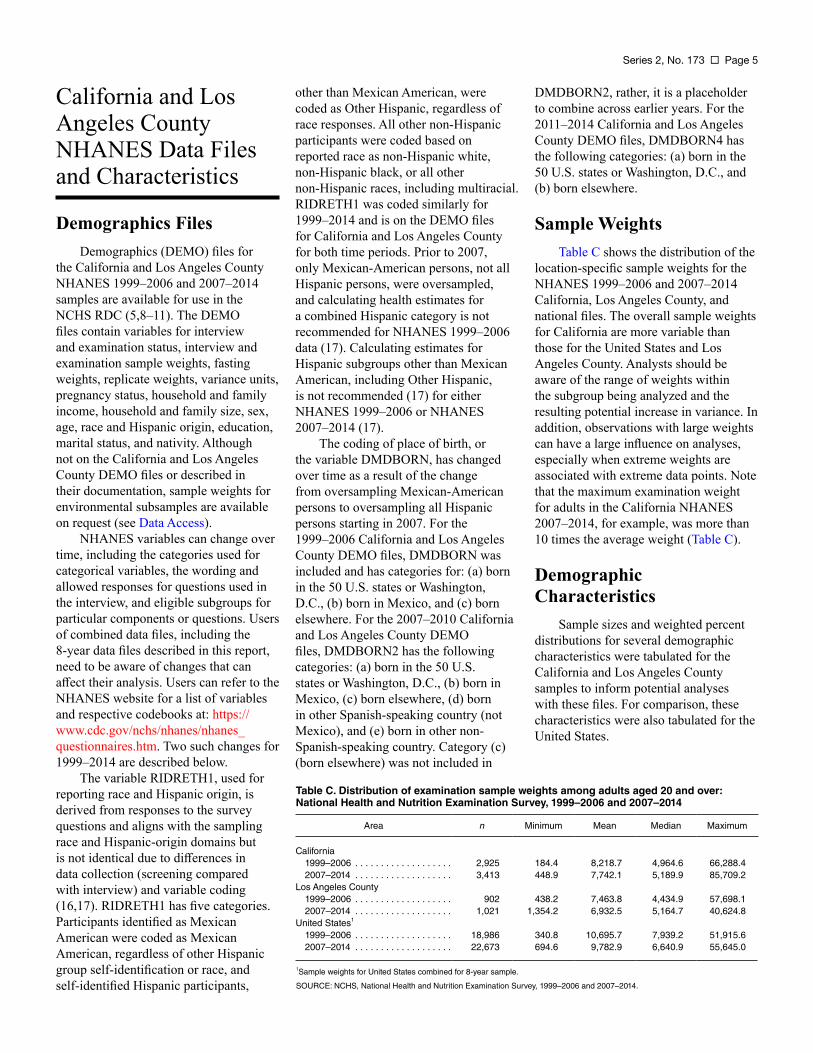
Sample WeightsTable C shows the distribution of the

location-specific sample weights for the NHANES 1999–2006 and 2007–2014 California, Los Angeles County, and national files. The overall sample weights for California are more variable than those for the United States and Los Angeles County. Analysts should be aware of the range of weights within the subgroup being analyzed and the resulting potential increase in variance. In addition, observations with large weights can have a large influence on analyses, especially when extreme weights are associated with extreme data points. Note that the maximum examination weight for adults in the California NHANES 2007–2014, for example, was more than 10 times the average weight (Table C).

Demographic Characteristics

Sample sizes and weighted percent distributions for several demographic characteristics were tabulated for the California and Los Angeles County samples to inform potential analyses with these files. For comparison, these characteristics were also tabulated for the United States.

Table C. Distribution of examination sample weights among adults aged 20 and over: National Health and Nutrition Examination Survey, 1999–2006 and 2007–2014

Area n Minimum Mean Median Maximum

California1999–2006 . . . . . . . . . . . . . . . . . . . 2,925 184.4 8,218.7 4,964.6 66,288.42007–2014 . . . . . . . . . . . . . . . . . . . 3,413 448.9 7,742.1 5,189.9 85,709.2

Los Angeles County1999–2006 . . . . . . . . . . . . . . . . . . . 902 438.2 7,463.8 4,434.9 57,698.12007–2014 . . . . . . . . . . . . . . . . . . . 1,021 1,354.2 6,932.5 5,164.7 40,624.8

United States1

1999–2006 . . . . . . . . . . . . . . . . . . . 18,986 340.8 10,695.7 7,939.2 51,915.62007–2014 . . . . . . . . . . . . . . . . . . . 22,673 694.6 9,782.9 6,640.9 55,645.0

1Sample weights for United States combined for 8-year sample.


https://www.cdc.gov/nchs/nhanes/nhanes_questionnaires.htm




For these tables, race and Hispanic origin was coded using RIDRETH1, as described above, into five categories for illustration: Mexican American, Other Hispanic, non-Hispanic white, non-Hispanic black, and all other non-Hispanic races, including multiracial. Although estimating health measures for the Other Hispanic and Other race groups is discouraged for NHANES 1999–2006 and NHANES 2007–2014, sample sizes and percentages for these categories were tabulated for this report for completeness. The ratio of family income to poverty, INDFMPIR, is based on the Department of Health and Human Services poverty guidelines (https://aspe.hhs.gov/poverty-guidelines) for eligibility for certain programs, such as the Supplemental Nutrition Assistance Program and Women, Infants, and Children. For this report, this variable was categorized as less than 1.3, greater than or equal to 1.3 but less than or equal to 3.5, or greater than 3.5. These cut points correspond to less than 130% of the federal poverty level (FPL), 130%–350% FPL, and greater than 350% FPL. Education for adults aged 20 and over (DMDEDUC2) was categorized as less than a high school graduate or General Educational Development (GED), a high school graduate or GED, and more than a high school graduate or GED. Country of birth, using DMDBORN for 1999–2006 and DMDBORN2 for 2007–2014, was coded into: (a) born in one of the 50 U.S. states or the District of Columbia, or (b) born in all other places.

Statements about unweighted sample sizes were not tested for statistical significance. Comparisons of population estimates of weighted percentages between California and the United States, between Los Angeles County and California, and between Los Angeles County and the United States were evaluated using two-sided z statistics at the 0.05 level.

Calculation of standard error (SE) for differences between estimates for overlapping geographic areas accounted for the population overlap between nested samples with the following expression:

SE(X1–X2) =

Var(X1) + Var(X2) – 2 • Var(X1) • N1

N2

where X2 is the estimate for the larger area, and X1 is the estimate for the smaller area within the larger area (e.g., Los Angeles County within California or California within the United States). N1 is the population size of the smaller area, and N2 is the population size of the larger area. This expression has been used to test differences between national and state estimates in prior NCHS health reports (19,20).

The Taylor Series Linearization method was used for variance estimation in SUDAAN (21) using the appropriate sample weights and variance units created for the California and Los Angeles County files, as described above, to produce subnational estimates and the sample weights and variance units from the national file to produce national estimates. Terms such as ‘‘greater than,’’ ‘‘less than,’’ ‘‘more likely,’’ or ‘‘less likely’’ indicate a statistically significant difference between estimates. Lack of comment regarding any difference does not mean that significance was tested and ruled out.

NHANES 1999–2006 California, Los Angeles County, and U.S. Samples

Sample sizes

Table D shows characteristics of the NHANES 1999–2006 interviewed and examined samples for California and Los Angeles County and the corresponding U.S. samples for both adults (aged 20 and over) and children (aged 0–19 years). As with the U.S. sample, slightly more children than adults were in the California and Los Angeles County samples. Of the 6,619 examined participants in the California 1999–2006 sample, 3,694 were children, and of the 2,155 examined participants in Los Angeles County, 1,253 were children.

Based on unweighted numbers, of the 902 interviewed and examined adults in Los Angeles County, nearly two-thirds (565) were Mexican American. Of the 2,925 adults interviewed and examined in California, over one-half (1,661) were Mexican American. In contrast, about 20% (unweighted) of the U.S. adult sample was Mexican American. Similarly, of the 1,253 interviewed and examined children in Los Angeles County, 968 were Mexican American and fewer than 70 were non-Hispanic white and 119 were non-Hispanic black. Among the 3,694 examined children in California, 2,783 were Mexican American. The large number of Mexican-American persons in the California and Los Angeles County samples was a result of the NHANES oversample of Mexican-American persons and the relatively high concentration of this group in California.

Demographic comparisons

For 1999–2006, the percentage of both adults and children below 130% FPL was higher for Los Angeles County (49.5% children, 33.5% adults) than for either the United States (33.5% children, 20.5% adults) or California (37.1% children, 19.6% adults) (Table D). Similarly, adults in Los Angeles County were more likely to have less than a high school education than adults in California or the United States. Compared with all children in the United States, more children in Los Angeles County and California were born outside of the United States. Similarly, nearly 50.0% of the adults in Los Angeles County were born outside of the United States compared with about one-third of California adults and 15.3% of U.S. adults. There were more Mexican-American children in Los Angeles County (43.7%) than in California (37.9%) and the United States (12.8%). Similarly, there were more Mexican-American adults in Los Angeles County (30.1%) compared with California (23.0%) and the United States (7.5%).

https://aspe.hhs.gov/poverty-guidelines

https://aspe.hhs.gov/poverty-guidelines


Table D. Sample sizes and weighted percent distributions of interviewed and examined adults and children: United States, California, and Los Angeles County National Health and Nutrition Examination Survey, 1999–2006

Characteristic

United States California Los Angeles County

n Percent SE n Percent SE n Percent SE

Adults aged 20 and over

All . . . . . . . . . . . . . . . . . . . . . . . . . . . . . . . . . . . . . 18,986 100.0 – 2,925 100.0 – 902 100.0 –

SexMale . . . . . . . . . . . . . . . . . . . . . . . . . . . . . . . . . 9,019 47.9 0.3 1,373 48.8 1.7 428 48.8 1.8Female . . . . . . . . . . . . . . . . . . . . . . . . . . . . . . . 9,967 52.1 0.3 1,552 51.2 1.7 474 51.2 1.8

Race and Hispanic originMexican American. . . . . . . . . . . . . . . . . . . . . . . 4,166 7.5 0.7 1,661 23.0 1.0 565 30.1 3.1Other Hispanic . . . . . . . . . . . . . . . . . . . . . . . . . 789 5.1 0.9 95 6.5 0.8 60 13.1 3.0Non-Hispanic white . . . . . . . . . . . . . . . . . . . . . . 9,485 71.5 1.4 820 54.7 1.9 119 36.4 4.8Non-Hispanic black . . . . . . . . . . . . . . . . . . . . . . 3,837 11.0 0.9 189 5.8 1.1 93 7.8 1.7Other race, including multiracial . . . . . . . . . . . . 709 4.9 0.4 160 10.0 1.2 65 12.7 1.8

Age20–39 . . . . . . . . . . . . . . . . . . . . . . . . . . . . . . . . 6,907 39.1 0.7 1,062 42.4 3.1 326 46.3 3.140–59 . . . . . . . . . . . . . . . . . . . . . . . . . . . . . . . . 5,607 38.2 0.6 872 38.9 2.6 273 36.5 2.960 and over . . . . . . . . . . . . . . . . . . . . . . . . . . . . 6,472 22.6 0.6 991 18.7 1.1 303 17.2 2.1

Poverty income ratioGreater than 0 but less than 1.3 . . . . . . . . . . . . 4,936 20.5 0.9 756 19.6 2.3 300 33.5 4.0Greater than or equal to 1.3 but less than or

equal to 3.5 . . . . . . . . . . . . . . . . . . . . . . . . . . . 6,873 37.1 0.7 1,091 34.1 2.4 331 37.1 3.9

Greater than 3.5 . . . . . . . . . . . . . . . . . . . . . . . . 5,690 42.4 1.2 812 46.3 3.8 164 29.4 4.6

EducationLess than high school . . . . . . . . . . . . . . . . . . . . 5,980 20.0 0.6 1,223 23.8 1.4 437 31.2 2.8High school diploma . . . . . . . . . . . . . . . . . . . . . 4,507 25.8 0.6 503 19.0 0.9 131 15.2 1.9More than high school. . . . . . . . . . . . . . . . . . . . 8,460 54.2 0.9 1,196 57.2 1.8 333 53.6 2.6

Country of birthBorn in United States . . . . . . . . . . . . . . . . . . . . 14,687 84.7 1.1 1,592 67.0 1.6 394 50.2 4.4Born outside United States . . . . . . . . . . . . . . . . 4,289 15.3 1.1 1,333 33.0 1.6 508 49.8 4.4

Children aged 0–19 years

All . . . . . . . . . . . . . . . . . . . . . . . . . . . . . . . . . . . . . 20,366 100.0 – 3,694 100.0 – 1,253 100.0 –

SexMale . . . . . . . . . . . . . . . . . . . . . . . . . . . . . . . . . 10,257 51.1 0.5 1,828 50.7 1.4 599 50.6 2.7Female . . . . . . . . . . . . . . . . . . . . . . . . . . . . . . . 10,109 48.9 0.5 1,866 49.3 1.4 654 49.4 2.7

Race and Hispanic originMexican American. . . . . . . . . . . . . . . . . . . . . . . 6,897 12.8 1.0 2,783 37.9 1.5 968 43.7 4.5Other Hispanic . . . . . . . . . . . . . . . . . . . . . . . . . 895 6.4 0.9 103 8.7 1.8 67 15.5 3.5Non-Hispanic white . . . . . . . . . . . . . . . . . . . . . . 5,543 59.6 1.7 387 35.2 2.2 62 22.0 3.9Non-Hispanic black . . . . . . . . . . . . . . . . . . . . . . 6,040 14.5 1.2 270 6.6 1.0 119 9.1 1.8Other race, including multiracial . . . . . . . . . . . . 991 6.8 0.6 151 11.7 1.5 37 9.8 2.8

Age group0–5 . . . . . . . . . . . . . . . . . . . . . . . . . . . . . . . . . . 6,818 29.3 0.5 1,175 29.6 1.3 410 29.3 2.06–11 . . . . . . . . . . . . . . . . . . . . . . . . . . . . . . . . . 4,361 30.2 0.6 778 30.8 1.0 279 31.5 3.012–19 . . . . . . . . . . . . . . . . . . . . . . . . . . . . . . . . 9,187 40.5 0.6 1,741 39.6 1.1 564 39.2 3.2

Poverty income ratioGreater than 0 but less than 1.3 . . . . . . . . . . . . 8,684 33.5 1.2 1,583 37.1 1.5 623 49.5 4.5Greater than or equal to 1.3 but less than or

equal to 3.5 . . . . . . . . . . . . . . . . . . . . . . . . . . . 6,600 37.4 0.9 1,209 31.9 2.0 350 25.8 3.3Greater than 3.5 . . . . . . . . . . . . . . . . . . . . . . . . 3,590 29.1 1.3 596 31.0 2.4 154 24.7 4.5

Country of birthBorn in United States . . . . . . . . . . . . . . . . . . . . 18,500 93.8 0.4 3,199 90.4 1.0 1,092 85.2 2.4Born outside United States . . . . . . . . . . . . . . . . 1,863 6.2 0.4 495 9.6 1.0 161 14.8 2.4

– Quanity zero.

NOTES: SE is standard error. Sample sizes may not sum to total due to missing data. Percent distributions were calculated excluding missing data.

SOURCE: NCHS, National Health and Nutrition Examination Survey, 1999–2006.


NHANES 2007–2014 California, Los Angeles County, and U.S. Samples

Sample sizes

There were 3,413 interviewed and examined adults and 2,675 children in the 2007–2014 California file and 1,021 interviewed and examined adults and 789 children in the 2007–2014 Los Angeles County file (Table E). Unlike the 1999–2006 file, slightly more adults than children were included in 2007–2014.

Of the 1,021 interviewed and examined adults in the 2007–2014 Los Angeles County file, about one-third (374) were Mexican American and 154 were in the Other Hispanic group. The change from the 1999–2006 file is due to the change in oversampling from Mexican-American to all Hispanic persons in 2007. Of the 3,413 adults interviewed and examined in California, 1,137 were Mexican American and 382 were in the Other Hispanic group. Compared with the 1999–2006 file, the number of adults in the Other race group in the 2007–2014 file increased to 718 in California and 213 in Los Angeles County due, in part, to the oversampling of Asian persons in 2011–2014.

Similarly, of the 789 interviewed and examined children in Los Angeles County, 434 were Mexican American and 117 were in the Other Hispanic group. Only 48 children were non-Hispanic white and 78 children were non-Hispanic black. Among the 2,675 children in California, 1,363 were Mexican American and 274 were in the Other Hispanic group.

Demographic comparisons

In 2007–2014, the percentage of adults and children below 130% FPL was higher for Los Angeles County than for the United States (Table E). Adults in Los Angeles County were more likely to have less than a high school education than adults in California or the United States. Compared with all children in the United States, more children in Los Angeles County and California were born outside of the United States. More than 50.0% of the adults in Los Angeles County were born outside of the United States

compared with more than one-third of California adults and 17.7% of U.S. adults. Close to one-half (48.2%) of children in Los Angeles County and 43.1% in California were Mexican American compared with 15.2% of children in the United States. Among adults, 30.8% of Los Angeles County adults were Mexican American compared with 25.2% in California and 8.5% in the United States.

Analytic IssuesGeneral guidelines for combining

NHANES files across survey cycles are in the NHANES Analytic Guidelines (16,17). Importantly, variables and variable formats frequently change over time for many reasons, including changes in the questionnaire, examination components, and sample design. For example, estimating health characteristics for all Hispanic persons was discouraged until the change in the sample design in 2007 that included oversampling all Hispanic persons. With an 8-year data file, analysts will need to confirm that the needed variables are available and can be consistently coded over the entire time period. Although the national sample weights and variance units can be merged to the California and Los Angeles County files, the national sample variables differ from those in the California- and Los Angeles County- specific NHANES DEMO files for the same participants, and the sample weights and variance units specific to California or Los Angeles County should be used for calculating subnational estimates.

The California and Los Angeles County data files span 8 years of data collection. Comparisons can be readily made to determine changes between 1999–2006 and 2007–2014. However, 8-year estimates are most appropriate for identifying relationships between risk factors and health outcomes that remain similar over the 8-year time periods. Estimates and associations for risk factors or health outcomes that may have changed within the 8-year time period may not be meaningful. Although year of examination is available in RDC, direct methods for estimating single-year

estimates and calculating annual trends from single-year estimates with the 8-year samples are not recommended, because the sample weights and variance units were not created for single-year estimates, and model-based approaches for estimating trends using the 8-year samples have not been evaluated.

The creation of sample weights for California was complicated by the NHANES sample designs, which were not intended to be used for subnational estimates. Locations selected for NHANES within California may have originally represented areas outside of California, and locations selected outside of California may have originally represented areas inside California. As a result, a combined design- and model-based approach was needed to create the California sample weights and variance units. The range of the resulting sample weights for California is wide, even within race and Hispanic origin groups. Variable and extreme weights can increase the standard errors of estimates and influence estimation, particularly when survey participants with very high sample weights also have extreme values of the health outcome of interest. In addition, variance units and replicates are provided on the California files for variance estimation. For calculating standard errors in this report, linearization methods were used for consistency across samples. For other analytic needs (e.g., regression, some statistical tests), replication methods are recommended for California data due to the composition of the California sample.

In 2000, about 40% of the Mexican-American and 30% of the Hispanic populations lived in California, and in 2010, about 35% of the Mexican-American and 28% of the Hispanic populations lived in California (22). The relatively large proportion of Mexican-American and other Hispanic persons from California, coupled with the NHANES design requirements for oversampling these groups within the small number of locations selected each cycle, led to the relatively large size of these groups in the California and Los Angeles County NHANES files. As a result, sample sizes for some of the


Table E. Sample sizes and weighted percent distributions of interviewed and examined adults and children: United States, California, and Los Angeles County National Health and Nutrition Examination Survey, 2007–2014

Characteristic

United States California Los Angeles County

n Percent SE n Percent SE n Percent SE

Adults aged 20 and over

All . . . . . . . . . . . . . . . . . . . . . . . . . . . . . . . . . . . . . . 22,673 100.0 – 3,413 100.0 – 1,021 100.0 –

SexMale . . . . . . . . . . . . . . . . . . . . . . . . . . . . . . . . . . 11,015 48.1 0.3 1,613 48.6 0.9 474 48.5 1.5Female . . . . . . . . . . . . . . . . . . . . . . . . . . . . . . . . 11,658 51.9 0.3 1,800 51.4 0.9 547 51.5 1.5

Race and Hispanic originMexican American. . . . . . . . . . . . . . . . . . . . . . . . 3,353 8.5 0.9 1,137 25.2 2.0 374 30.8 2.6Other Hispanic . . . . . . . . . . . . . . . . . . . . . . . . . . 2,284 5.5 0.6 382 7.4 1.1 154 11.8 1.4Non-Hispanic white . . . . . . . . . . . . . . . . . . . . . . . 9,926 67.4 1.8 790 44.7 2.7 165 31.6 3.0Non-Hispanic black . . . . . . . . . . . . . . . . . . . . . . . 4,831 11.4 0.9 386 5.9 1.1 115 8.7 1.2Other race, including multiracial . . . . . . . . . . . . . 2,279 7.3 0.5 718 16.7 1.6 213 17.1 2.9

Age20–39 . . . . . . . . . . . . . . . . . . . . . . . . . . . . . . . . . 7,635 36.8 0.8 1,151 39.5 1.9 334 41.5 3.040–59 . . . . . . . . . . . . . . . . . . . . . . . . . . . . . . . . . 7,516 38.0 0.5 1,174 37.6 1.4 347 37.3 2.460 and over . . . . . . . . . . . . . . . . . . . . . . . . . . . . . 7,522 25.3 0.5 1,088 22.9 1.4 340 21.3 2.5

Poverty income ratioGreater than 0 but less than 1.3 . . . . . . . . . . . . . 6,968 23.1 0.9 908 23.1 2.0 307 28.8 2.6Greater than or equal to 1.3 but less than or

equal to 3.5 . . . . . . . . . . . . . . . . . . . . . . . . . . . .7,517 35.2 0.7 1,087 35.7 2.5 344 37.6 3.4

Greater than 3.5 . . . . . . . . . . . . . . . . . . . . . . . . . 6,185 41.7 1.2 990 41.2 1.9 213 33.6 3.1

EducationLess than high school . . . . . . . . . . . . . . . . . . . . . 5,963 17.9 0.8 1,053 23.3 1.4 383 30.4 2.7High school diploma . . . . . . . . . . . . . . . . . . . . . . 5,177 22.5 0.6 584 15.8 0.8 190 16.6 1.5More than high school. . . . . . . . . . . . . . . . . . . . . 11,504 59.6 1.1 1,771 60.8 1.8 447 53.1 2.9

Country of birthBorn in United States . . . . . . . . . . . . . . . . . . . . . 16,319 82.3 1.1 1,749 64.2 2.1 406 49.0 2.5Born outside United States . . . . . . . . . . . . . . . . . 6,341 17.7 1.1 1,659 35.8 2.1 613 51.0 2.5

Children aged 0–19 years

All . . . . . . . . . . . . . . . . . . . . . . . . . . . . . . . . . . . . . . 16,493 100.0 – 2,675 100.0 – 789 100.0 –

SexMale . . . . . . . . . . . . . . . . . . . . . . . . . . . . . . . . . . 8,472 51.1 0.6 1,347 51.1 1.4 385 51.0 3.0Female . . . . . . . . . . . . . . . . . . . . . . . . . . . . . . . . 8,021 48.9 0.6 1,328 48.9 1.4 404 49.0 3.0

Race and Hispanic originMexican American. . . . . . . . . . . . . . . . . . . . . . . . 4,017 15.2 1.4 1,363 43.1 2.7 434 48.2 3.5Other Hispanic . . . . . . . . . . . . . . . . . . . . . . . . . . 1,907 7.2 0.8 274 7.6 0.7 117 13.3 1.7Non-Hispanic white . . . . . . . . . . . . . . . . . . . . . . . 4,739 54.9 2.2 304 27.6 2.1 48 14.4 2.9Non-Hispanic black . . . . . . . . . . . . . . . . . . . . . . . 3,993 14.3 1.1 291 6.5 1.5 78 8.3 1.4Other race, including multiracial . . . . . . . . . . . . . 1,837 8.4 0.5 443 15.3 1.4 112 15.8 4.0

Age (years)0–5 . . . . . . . . . . . . . . . . . . . . . . . . . . . . . . . . . . . 6,331 29.8 0.6 951 29.4 1.7 275 29.2 2.66–11 . . . . . . . . . . . . . . . . . . . . . . . . . . . . . . . . . . 5,021 29.5 0.5 789 29.0 1.4 241 28.2 1.712–19 . . . . . . . . . . . . . . . . . . . . . . . . . . . . . . . . . 5,141 40.7 0.7 935 41.5 2.5 273 42.6 2.3

Poverty income ratioGreater than 0 but less than 1.3 . . . . . . . . . . . . . 7,299 35.4 1.4 1,073 39.3 3.3 360 47.5 3.9Greater than or equal to 1.3 but less than or

equal to 3.5 . . . . . . . . . . . . . . . . . . . . . . . . . . . .5,016 35.3 0.9 817 35.6 3.2 218 31.3 4.3

Greater than 3.5 . . . . . . . . . . . . . . . . . . . . . . . . . 2,897 29.3 1.4 481 25.1 3.6 95 21.2 3.5

Country of birthBorn in United States . . . . . . . . . . . . . . . . . . . . . 15,392 94.4 0.4 2,448 90.8 1.6 729 90.4 2.7Born outside United States . . . . . . . . . . . . . . . . . 1,094 5.6 0.4 223 9.2 1.6 60 9.6 2.7

– Quanity zero.

NOTES: SE is standard error. Sample sizes may not sum to total due to missing data. Percent distributions were calculated excluding missing data.



other race and Hispanic-origin groups, particularly non-Hispanic black persons, are relatively small, and the estimates derived from these smaller demographic subgroups may not be reliable when stratified by age group, sex, or other characteristics.

Data AccessThe California and Los Angeles

County NHANES data files are available in the NCHS RDC (5). To use these files, analysts should follow the guidance provided on the NCHS RDC website (https://www.cdc.gov/rdc/index.htm). Briefly, analysts should submit proposals to RDC outlining their research objectives, including the variables needed, the structure of the analytic file, and the proposed tabular results to leave RDC. Although the DEMO files have been created for California and Los Angeles County, most research using these files will require merging health variables from NHANES national files for different years, which will need to be described in the proposal. Projects requiring sample weights not listed in the DEMO file documentation, such as weights for a one-third subsample, should indicate this need on the RDC proposal.

Summary

These files demonstrate that subnational estimates can be made by combining several years of NHANES data and using the original sample design information as a starting point for creating location-specific variance units and sample weights. California is the most populous state and, as a result, has included many NHANES PSUs since 1999. Similarly, Los Angeles County is the only county to be included with certainty for each of the NHANES sample designs. Even so, many years of data were needed to create data files for these locations that would have sufficient precision. Nevertheless, the NHANES 1999–2006 and 2007–2014 California and Los Angeles County files provide an opportunity to examine factors associated with health and nutrition for these locations.

References

1. National Health and Nutrition Examination Survey. Available from: https://www.cdc.gov/nchs/nhanes/index.htm.

2. U.S. Census Bureau. QuickFacts: California. Available from: https://www.census.gov/quickfacts/table/PST045215/06.

3. Mackun P, Wilson S. Population distribution and change: 2000 to 2010. 2010 Census Briefs. 2011. Available from: https://www.census.gov/prod/cen2010/briefs/c2010br-01.pdf.

4. Humes KR, Jones NA, Ramirez RR. Overview of race and Hispanic origin: 2010. 2010 Census Briefs. 2011. Available from: https://www.census.gov/prod/cen2010/briefs/c2010br-02.pdf.

5. National Center for Health Statistics. Research Data Center. Available from: https://www.cdc.gov/rdc/index.htm.

6. Porter KS, Curtin LR, Carroll MD, et al. Health of adults in Los Angeles County: Findings from the National Health and Nutrition Examination Survey, 1999–2004. National health statistics reports; no 42. Hyattsville, MD: National Center for Health Statistics. 2011.

7. Kruszon-Moran D, Porter KS, McQuillan G, et al. Infectious disease prevalence in Los Angeles County—A comparison to national estimates, 1999–2004. NCHS data brief, no 90. Hyattsville, MD: National Center for Health Statistics. 2012.

8. National Center for Health Statistics. National Health and Nutrition Examination Survey 1999–2006 data documentation, codebook, and frequencies. California—Demographic variables & sample weights (CDEMO_AD). 2016. Available from: https://wwwn.cdc.gov/Nchs/Nhanes/limited_access/CDEMO_AD.htm.

9. National Center for Health Statistics. National Health and Nutrition Examination Survey 2007–2014 data documentation, codebook,

and frequencies. California—Demographic variables & sample weights (CDEMO_EH). 2015. Available from: https://wwwn.cdc.gov/Nchs/Nhanes/limited_access/CDEMO_EH.htm.

10. National Center for Health Statistics. National Health and Nutrition Examination Survey 1999–2006 data documentation, codebook, and frequencies. Los Angeles County, California—Demographic variables & sample weights (LDEMO_AD). 2015. Available from: https://wwwn.cdc.gov/Nchs/Nhanes/limited_access/LDEMO_AD.htm.

11. National Center for Health Statistics. National Health and Nutrition Examination Survey 2007–2014 data documentation, codebook, and frequencies. Los Angeles County, California—Demographic variables & sample weights (LDEMO_EH). 2015. Available from: https://wwwn.cdc.gov/Nchs/Nhanes/limited_access/LDEMO_EH.htm.

12. Curtin LR, Mohadjer L, Dohrmann S, et al. The National Health and Nutrition Examination Survey: Sample design, 1999–2006. National Center for Health Statistics. Vital Health Stat 2(155). 2012. Available from: https://www.cdc.gov/nchs/data/series/sr_02/sr02_155.pdf.

13. Curtin LR, Mohadjer LK, Dohrmann SM, et al. National Health and Nutrition Examination Survey: Sample design, 2007–2010. National Center for Health Statistics. Vital Health Stat 2(160). 2013. Available from: https://www.cdc.gov/nchs/data/series/sr_02/sr02_160.pdf.

14. Johnson CL, Dohrmann SM, Burt VL, Mohadjer LK. National Health and Nutrition Examination Survey: Sample design, 2011–2014. National Center for Health Statistics. Vital Health Stat 2(162). 2014. Available from: https://www.cdc.gov/nchs/data/series/sr_02/sr02_162.pdf.

15. Mirel LB, Mohadjer LK, Dohrmann SM, et al. National Health and Nutrition Examination Survey: Estimation procedures, 2007–2010. National Center for Health Statistics. Vital Health Stat 2(159). 2013.

https://www.cdc.gov/rdc/index.htm


https://www.cdc.gov/nchs/nhanes/index.htm

https://www.cdc.gov/nchs/nhanes/index.htm

https://www.census.gov/quickfacts/table/PST045215/06

https://www.census.gov/quickfacts/table/PST045215/06

https://www.census.gov/prod/cen2010/briefs/c2010br-01.pdf








https://wwwn.cdc.gov/Nchs/Nhanes/limited_access/CDEMO_AD.htm



https://wwwn.cdc.gov/Nchs/Nhanes/limited_access/CDEMO_EH.htm



https://wwwn.cdc.gov/Nchs/Nhanes/limited_access/LDEMO_AD.htm



https://wwwn.cdc.gov/Nchs/Nhanes/limited_access/LDEMO_EH.htm



https://www.cdc.gov/nchs/data/series/sr_02/sr02_155.pdf








Available from: https://www.cdc.gov/nchs/data/series/sr_02/sr02_159.pdf.

16. Johnson CL, Paulose-Ram R, Ogden CL, et al. National Health and Nutrition Examination Survey: Analytic Guidelines, 1999–2010. National Center for Health Statistics. Vital Health Stat 2(161). 2013. Available from: https://www.cdc.gov/nchs/data/series/sr_02/sr02_161.pdf.

17. National Center for Health Statistics. National Health and Nutrition Examination Survey: Analytic guidelines, 2011–2012. 2013. Available from: https://www.cdc.gov/nchs/data/nhanes/analytic_guidelines_11_12.pdf.

18. Fay RE. Theory and application of replicate weighting for variance calculations. Proceedings of the section on survey research methods, American Statistical Association, 212–7. 1989.

19. Cohen RA, Martinez ME. Health insurance coverage: Early release of estimates from the National Health Interview Survey, 2014. National Center for Health Statistics. June 2015.

20. Bramlett MD, Blumberg SJ. Prevalence of children with special health care needs in metropolitan and micropolitan statistical areas in the United States. Matern Child Health J 12(4):488–98. 2008.

21. RTI International. SUDAAN (Release 11.0.0) [computer software]. 2012.

22. Ennis SR, Ríos-Vargas M, Albert NG. The Hispanic population: 2010. 2010 Census Briefs. 2011.







https://www.cdc.gov/nchs/data/nhanes/analytic_guidelines_11_12.pdf




Appendix. Background: California Sample Weights, 1999–2006

The development of state level estimates for the National Health and Nutrition Examination Survey (NHANES) began with California. California is a large and populous state that was sampled multiple times in each NHANES design. A handful of alternatives for creating state-level sample weights for California from multiple NHANES cycles were considered before the decision was made to combine 8 years of data. This Appendix describes the methods used for the final California NHANES 1999–2006 sample weights. The creation of the California NHANES 2007–2014 sample weights followed a similar process with differences described in the main text.

The computation of the California NHANES 1999–2006 weights began by converting national base weights (based on each sampled person’s selection probability) to state-level base weights. National weights were created for the following 2-year periods: 1999–2000, 2001–2002, 2003–2004, and 2005–2006. These periods were spanned by two different sample designs: a 6-year design for 1999–2004, where the last 3 years were dropped, and a 6-year design for 2002–2007, where the last year was not implemented but was instead replaced by a design for 2007–2010. Several factors contributed to the decision to change these sample designs, including the cost effectiveness of meeting target sample sizes for specific subgroups using the original 1999–2004 design and the decision to release data files every 2 years instead of every 3 years.

The sampling frame and sampling rates differed under the two designs. Under the 1999–2004 design, the 1995–2004 National Health Interview Survey counties served as the sampling frame for the selection of NHANES primary sampling units (PSUs). The PSU measure of size (MOS) and the overall sampling rates were based on Census 1990 population totals and population projections for the year 2000. Under the 2002–2007 design, PSUs were sampled from all counties in the nation. The MOS and overall sampling rates were based

on Census 2000 population totals and population projections for 2004.

Under both designs, the NHANES sample was selected in four stages. In the first stage, PSUs, which are counties or groups of counties, were sampled with probabilities proportionate to size (PPS). Then, segments (Census blocks or groups of blocks) were selected with PPS within each PSU, and a random sample of dwelling units was taken in each segment. Finally, one or more persons were sampled within a dwelling unit (DU) to achieve the desired sampling rate for the domain (defined by age, sex, race and ethnicity, and income). Thus, the original base weight for a sampled person (SP) is the reciprocal of the sampling rate for the sampling domain of the SP.

When calculating any multiyear sample weight, the original base weight was adjusted to account for (a) the proportion of DUs released, (b) the proportion of deselected DUs, (c) the number of newly constructed DUs completed between DU sample selection and data collection (NHANES 1999 and the first four stands in NHANES 2000 used new construction segment sampling), and (d) the number of years in the sample.

The effect of the first-stage selection of PSUs can be separated from the remaining stages of selection by expressing the national base weight, whi(BASE)

0 , for SP i in PSU h as

yriw = wh(national) •hi(BASE)

0whi

w

where

wh(national) = the PSU weight to produce single-year national estimates;

whiw = a within-PSU weight reflecting

all stages of sampling (segments, DUs, and SPs) within the PSU, conditional on the PSU’s selection; and

yri = the number of years in the weighting sample containing SP i.

(Because the computations described here are based on national weights for 2-year periods, yri = 2 for each i.)

In turn, wh(national) = 1 ⁄ ph1 where

ph1 = the selection probability of PSU h in

a single year, and

=ph1

mh

ph(national)c

where

ph(national)c = the probability of selection of

the PSU over the duration of the original design (1999–2004 or 2002–2007); and

1 ⁄ mh = the probability of selection of PSU h for a given year in the span of the original design.

Thus, a 1-year within-PSU weight, whi

w , conditional on the selection of the PSU in a given year, may be computed as

wh(national)= yri •

= yri •

whiw

mh

ph(national)c

0• whi(BASE)

0whi(BASE)

Typically, mh = 6. For 1999–2006, the values of mh were adjusted to compensate for special adjustments incorporated into the national weights for those years. The 1999–2004 design was initially developed with the target of 20 stands per year or 120 overall, but a subsample at 14 per year was also developed in anticipation of a smaller NHANES. The design evolved and later calculations reflected a reduction to 12 stands in 1999 and 15 in subsequent years. The reduction of 3 stands in 1999, or 87 instead of 90 over the projected 6-year interval, was reflected by an adjustment to the weights in both certainty and noncertainty PSUs. In place of mh = 6, single-year weights were adjusted by a factor of 7.25 (= 6 • 15/12 • 87/90) in 1999 and 5.8 (= 6 • 87/90) in 2000 and 2001.

California PSU WeightsAs described above, the national base

weights are the product of the inverse of the PSU selection probability for the national sample and the inverse within-PSU selection probability, adjusted by the number of years in the weighting


sample. To represent California for the 8-year period for 1999–2006, weights at the PSU level were produced to reflect the PSU probability of selection within California. This was done by using the framework of the 2002–2007 design to implement an estimator that was design based to the extent possible. Then, initial person-level weights (base weights) were created from the California PSU weights and the within-PSU selection probabilities.

PSU weights for certainty PSUsBecause all of the California

certainty PSUs in the original 2002–2007 sample were in the final 1999–2006 sample, a conditional approach (e.g., Rao 1985) was used to develop PSU weights for the certainty PSUs. The PSUs selected with a probability of 1 in the original NHANES 2002–2007 sample were treated as certainty for the purpose of creating weights for California during 1999–2006. The PSU weight for a particular PSU was assigned conditionally on the inclusion of the certainty PSU in the years 1999–2006 and the number of times it was in the sample during that period. For PSU h, this can be expressed as:

wh(state) = kh

1

where

wh(state) = the PSU weight to produce California estimates, and

kh = the number of times PSU h was in the sample during 1999–2006.

The values of the PSU weights for the certainty PSUs range from 0.3 to 1.0.

As noted above, the assignment of the PSU weights in this manner followed a conditional inference approach based on the arguments in Rao (1985). The calculation addresses the fact that not all sections of Los Angeles County were included in the sample the same number of times. Also, if unconditional weights were computed, based on the expected number of times that the PSUs selected for the original 2002–2007 sample were in the final sample, it would have been necessary to estimate between-PSU variance for these PSUs. The conditional weighting advantageously eliminates the

between-PSU variance for these certainty PSUs.

PSU weights for noncertaintyTo deal with the non-certainty

strata without sampled California counties, a quasi-modeling approach was implemented. The California PSU weights for the non-certainty counties in California in 2002–2006 were based on the national sample design, to the extent possible. The PSUs were assigned the same MOS and strata as in the national sample for 2002–2007. The California PSUs sampled in 1999–2001 were then treated as if they had been sampled under the 2002–2007 design. In other words, they were assigned the MOS and stratum from the latter design.

The national 2002–2007 sample included one PSU per minor stratum, and each annual sample contained one PSU per major stratum, where the major strata are defined by grouping six minor strata with similar demographics. Because some of the strata contained no sampled PSUs in California over the full 8-year period, some collapsing of strata was necessary.

Two options were considered for collapsing. One was to collapse to the major strata level. The other involved preserving as many minor strata as possible. While collapsing to the major strata level could have the advantage of less variation in the weights, the National Center for Health Statistics decided to use the option with more limited collapsing. This was done to take better advantage of the stratification to the extent that non-sampled PSUs in a minor stratum are more similar to sampled PSUs in the same minor stratum than those in other minor strata in the same major stratum. Under this option, no collapsing was needed for metropolitan statistical area (MSA) strata with a high proportion of Mexican-American people. No non-MSA strata contained sampled California PSUs, and some low Mexican-American MSA strata were also empty, therefore, some collapsing was needed over these groups.

The PSU weights for the non-certainties were then calculated using these collapsed strata as:

wh(state) = kh nH' MOSh

∑j∈H' MOSj1

where

H' = all California PSUs in the collapsed stratum containing PSU h,

MOSj = the measure of size of PSU j, where j ϵ H',

nH' = the number of California PSUs in the collapsed stratum H' in the sample during 1999–2006, and

kh = 2 for the noncertainty PSUs that were sampled in both 1999–2001 and 2002–2006, and 1 otherwise.

This is similar to the calculation of PSU weights in the national PPS sample. However, the weight was modified to reflect the reciprocal probability of selection within California. The PSU weights for non-certainties ranged from approximately 0.6 to 8.7.

California Base WeightsThe initial California SP weights

were then created from the national base weights by factoring out the PSU weights for the national sample and applying the PSU weights for California. The California base weight, whi(BASE), can be derived from the 1-year within-PSU weight, whi

w , and the California PSU weight, wh(state), according to the following formula:

wwhi(BASE) = wh(state) • whi

= yri • mh

ph(national)c

0= fstate • whi(BASE)

0• wh(state) • whi(BASE)

The factors, fstate, that were applied to the national base weights, 0whi(BASE), to create California base weights, whi(BASE), range from 0.1 to 0.6.

Computation of Final Weights

Nonres ponse adjustmentSome of the SPs who were

screened refused to be interviewed (interview nonresponse), and some of


the interviewed SPs refused the medical examination (examination nonresponse). Thus, nonresponse bias may result. Bias in the survey estimates occurs when the characteristics of nonrespondents are very different from those of respondents. The best approach to minimizing nonresponse bias is to plan and implement field procedures that maintain high cooperation rates. For NHANES, the payment of cash incentives and repeated callbacks for refusal conversion are very effective in reducing nonresponse and, thus, nonresponse bias. However, some nonresponse occurs even with the best strategies. Therefore, adjustments are always necessary to minimize potential nonresponse bias.

For the national weights, a multistage procedure for nonresponse adjustment is carried out to adjust for unit nonresponse in NHANES for each stage of nonresponse. The same procedure was used for the California weights to adjust for nonresponse within California. The nonresponse adjustment procedure consists of computing adjustment factors and applying these factors to the survey weights separately by nonresponse cell. Nonresponse adjustment reduces bias if response rates and survey characteristics vary from cell to cell and respondents and nonrespondents sharing the same characteristics are in the same cell. The nonresponse adjustment factors are the reciprocals of the weighted response rates within the selected cells.

A negative effect of nonresponse adjustment is that it increases the variability of the weights, which in turn increases sampling variance. When the nonresponse cells contain a sufficient number of cases and the adjustment factors are not too large, the effect on variances is modest. A large adjustment factor in a cell is usually the result of the small number of respondents in that cell. To avoid having nonresponse adjustments based on very small sample sizes or having large nonresponse adjustment factors, cells are usually collapsed to form larger cells. The following criteria were used for the California weights to determine whether to collapse cells:

● Minimum of 30 respondents in each cell

● Maximum adjustment factor of 1.35

However, in some cases in which the combining of cells to reach a lower adjustment factor led to overly large cells or otherwise impractical cell definitions, larger nonresponse factors were permitted.

Nonresponse adjustments were carried out separately for screener nonresponse, interview nonresponse, and examination nonresponse. For the screener nonresponse adjustment of the national weights, cells were defined by segments within each location. Therefore, all cases from California were in cells with other cases in the same location. Thus, the screener nonresponse adjustment factors, fi(NR,s), were the same for California weights and national weights.

For the interview and examination nonresponse adjustments, variables related to response propensity were identified using the Chi-squared Automatic Interaction Detector (CHAID). The CHAID is a classification algorithm that uses the likelihood ratio chi-square to divide a population into homogeneous subgroups with respect to a target characteristic (in this case, response rates). The same sets of variables were considered as in the weighting for the 1999–2000, 2001–2002, 2003–2004, and 2005–2006 national samples along with the addition of a time variable. To avoid too fine a division of the data, time was treated as a dichotomy, 1999–2002 compared with 2003–2006. For both the interview and examination adjustments, given the possible interest in analyzing Los Angeles County separately, separate nonresponse adjustment cells were developed for persons sampled in Los Angeles County and those in other survey locations within four age groups (0–5, 6–19, 20–59, and 60 and over).

The nonresponse adjustment factors, fi(NR), were calculated as follows:

fi(NR) =∑i=1 wi(BASE)

∑i=1 wi(BASE)

nas

nar

where wi(BASE) is the base weight for the ith SP in the ath cell, nas is the total sample size in the ath nonresponse

adjustment cell, and nar is the number of respondents in the a–th cell. The summation was carried out separately for each cell. Cells were collapsed with other cells to reduce any large factors. Thus, the nonresponse-adjusted weights, wi(NR), were calculated as follows:

wi(NR) = wi(BASE) fi(NR)

Interview: Variables considered for nonresponse adjustment

Of the 8,826 identified sampled persons, 6,979 (or 79.1%) responded to the interview. The analysis performed at the interview level showed that different variables were related to response propensity depending on the age of the sampled person (in the following order):

● Aged 0–5 years: Race and ethnicity of the respondent (Mexican American, black, and white or other) and household size (1–4 persons, 5–6 persons, and 7 or more persons).

● Aged 6–19 years: Household size (1–4 persons, 5–6 persons, and 7 or more persons) and race and ethnicity of the respondent (Mexican American, white, and black or other).

● Aged 20–59: Indicator whether any kids aged 1 through 5 years were sampled in the household, race and ethnicity of the respondent (Mexican American, white, and black or other), indicator whether any kids younger than 16 were sampled in the household, and household size (1–3 persons and 4 or more persons).

● Aged 60 and over: Year in sample (1999–2002 and 2003–2006).

The interview nonresponse adjustment factors ranged from 1.00 (no adjustment) to 1.65.

Mobile Examination Center examination: Variables considered for nonresponse adjustment

A total of 6,619 (or 94.8%) of the 6,979 interview respondents completed a Mobile Examination Center (MEC) examination. The results from the chi-square classification analysis again showed that different variables were related to response propensity depending on the age of the SP (in the following order):


● Aged 0–5 years: Number of SPs in the household (1–2 and 3 or more).

● Aged 6–19 years: Household size (1–3 persons and 4 or more persons), education level of respondent (less than high school or unknown and high school or more), and household SP composition (all SPs under age 16, all SPs aged 16 and over, and mixed ages).

● Aged 20–59: Self-reported health of the SP (excellent or unknown, very good or good, and fair or poor), number of SPs in the household (one and two or more), length of stay at current residence (5 years or less or unknown and more than 5 years), and indicator whether any kids aged 1–5 years were sampled in the household.

● Aged 60 and over: Self-reported health of the SP (excellent or unknown; very good, good, or fair; and poor) and year in sample (1999–2002 and 2003–2006).

The MEC examination nonresponse adjustment factors ranged from 1.00 (no adjustment) to 1.27.

TrimmingNonresponse adjustments can

contribute to extreme weights. Therefore, trimming of the weights was considered. Extreme weights may also occur when units are sampled to yield fixed sample sizes within a PSU, as was the case in NHANES. In addition, the adjustments required to create state-level estimates introduced additional variability into the weights. Even a few unexpectedly large sampling weights can seriously inflate the variance of survey estimates. Thus, weight trimming procedures may be used to reduce the impact of any such large SP weights on the estimates produced from the sample.

Trimming introduces a bias in the estimates but a reduction in their variances. The reduction in variance may decrease the mean squared error. The inspection method was used for trimming the California weights, which is the same procedure used for the national weights. This method involves inspecting the distribution of weights in the sample and

applies to samples (or subsets of samples) that were originally designed to be self-weighting.

The subdomains for trimming are the race-ethnicity-sex-age-income and pregnancy sampling domains. Because Mexican-American persons, pregnant women, and white and other persons with low income (beginning in 2000) were oversampled in NHANES, the weights in their domains may be quite variable. For this reason, trimming thresholds were dependent on the amount of oversampling used in these domains.

After the weights to be trimmed were identified, the weights of the nontrimmed cases were also adjusted, so the weights for each sampling domain and reason for selection (e.g., income or pregnancy) summed to the corresponding weighted sum prior to trimming. This is referred to as “preserving weighted totals.” Failure to preserve weighted totals may lead to serious understatements in estimated totals; thus, this is an important characteristic to have in a trimming procedure.

The trimming factors, fi(TR), were calculated as follows:

fi(TR) =∑i=1 ti

nb

∑i=1 wi(BASE) fi(NR)nb

where nb is the sample size of the bth race-ethnicity-sex-age-income and pregnancy sampling domain, and ti is equal to wi(BASE) fi(NR), provided that this product does not exceed the threshold and is set to be equal to the threshold otherwise. The trimmed weights, wi(TR), were calculated as follows:

wi(TR) = wi(NR) fi(TR)

Trimming thresholds were based on the same criteria as national weights for these years. Among the Mexican-American women selected because they were in the pregnant category, the weight was trimmed if it exceeded 6.5 times the mean weight for women in the race-ethnicity-sex-age domain. Weights for all other Mexican-American persons were trimmed if they exceeded 4.5 times the mean weight for persons in the race-ethnicity-sex-age domain. For the non-Mexican-American women selected

because they were in the pregnant category, weights were trimmed if they exceeded five times the mean weight for women in the race-ethnicity-sex-age domain. For the white and other persons selected because they were in the low income category, weights were trimmed if they exceeded four times the mean weight for persons in the race-ethnicity-sex-age domain. All other weights were trimmed if they exceeded three times the race-ethnicity-sex-age domain mean.

PoststratificationThe final step in the weighting

procedure was poststratification to known population totals to compensate for undercoverage or overcoverage of certain demographic groups and for any residual differential nonresponse among these groups. Poststratification of sample weights to independent population estimates is used for several purposes. In most household surveys, certain demographic groups in the U.S. population (e.g., young black males) experience fairly high rates of undercoverage in survey efforts. Poststratification to census estimates partially compensates for such undercoverage and for any differential nonresponse and can help to reduce the resulting bias in the survey estimates. It can also help to reduce the variability of sample estimates. Because the NHANES sample was a national sample and not designed to be representative of the California population, poststratification is also used to achieve consistency with accepted totals for various subpopulations in California. In particular, it partly addresses the disproportionate number of Mexican-American persons.

Poststratification involves applying a ratio adjustment to the survey weights. Broad classes, called poststratification cells or poststrata, are constructed using auxiliary data, and a single ratio adjustment factor is applied to all units in a given poststratification cell. The numerator of the ratio is a “control total” obtained from a secondary source. The denominator is a weighted total obtained using the survey weights. Therefore, at the poststratum level, estimates obtained using the poststratified survey weights


will correspond to the control totals used. Because poststratification is a ratio adjustment, this process will improve the efficiency of estimates provided the variables used in constructing poststratification cells are associated with the analysis variables of interest. Such gains in efficiency are most evident in the case of linear estimates, such as means or totals. For ratio estimates, the ratio adjustments cancel each other out at the poststratum level, and the overall gains in efficiency due to poststratification tend to be small.

A major effect of poststratification is that it implicitly imputes for unit nonresponse of survey characteristics for the missed persons. The assumption is that these missed persons not covered by the survey have the same distribution of characteristics as interviewed persons within the poststratification cells. This is obviously an oversimplification; the missed persons are likely to be different. However, in the absence of any detailed information on the characteristics of the

missed persons, poststratification appears to be the only reasonable technique available for reducing the bias due to undercoverage and nonresponse.

Control totals for California were first derived for the 1999–2002 sample and the 2003–2006 sample, and then the counts for the two 4-year samples were averaged to create control totals for the 1999–2006 California sample. For the 1999–2002 California sample, the counts were obtained from the Census 2000 Public Use Microdata Sample (PUMS). This file includes totals for the noninstitutionalized civilian population in California for the year 2000, approximately the middle of the 4-year time period. For the 2003–2006 California sample control totals, the 2005 American Community Survey (ACS) was used. The 2005 ACS did not include the group quarter population, so estimates of the California civilian household (nongroup quarter) population were inflated by the 2006 ACS ratio of the noninstitutionalized civilian population

to the civilian household population for California. The poststratification, therefore, will bring the weighted totals up to the level of the presumed total noninstitutionalized civilian population in California (Table).

The poststratification factors, fi(PS), were calculated as follows:

fi(PS) =Nc

∑i=1 wi(TR)nc

where Nc is the control total, and nc is the sample size of the poststratification cell. Thus, the poststratified weights, wi(PS), were calculated as follows:

wi(PS) = wi(NR) fi(PS)

Postratification adjustment factors

The screener-level poststratification adjustment factors ranged from 0.99 to 1.30. The interview-level poststratification adjustment factors ranged from 0.94 to 1.03. The MEC

Table. Control totals for noninstitutionalized civilian population, by domain: California National Health and Nutrition Examination Survey, 1999–2006

Race and ethnicity-sex-age sampling domainsPopulation from 2000 Public

Use Microdata SamplePopulation from 2005 American

Community Survey11999–2006

control totals

Black

Male and female0–5 years . . . . . . . . . . . . . . . . . . . . . . . . . . . . . . . . . . . . . . . . . . . 241,308 234,988 238,148

Male6–19 years . . . . . . . . . . . . . . . . . . . . . . . . . . . . . . . . . . . . . . . . . . 297,678 299,249 298,46420 and over . . . . . . . . . . . . . . . . . . . . . . . . . . . . . . . . . . . . . . . . . . 682,506 704,350 693,428

Female6–19 years . . . . . . . . . . . . . . . . . . . . . . . . . . . . . . . . . . . . . . . . . . 288,069 301,768 294,91820 and over . . . . . . . . . . . . . . . . . . . . . . . . . . . . . . . . . . . . . . . . . . 802,556 825,377 813,967

Mexican American

Male and female0–5 years . . . . . . . . . . . . . . . . . . . . . . . . . . . . . . . . . . . . . . . . . . . 1,162,519 1,390,831 1,276,675

Male6–19 years . . . . . . . . . . . . . . . . . . . . . . . . . . . . . . . . . . . . . . . . . . 1,259,302 1,467,888 1,363,59520 and over . . . . . . . . . . . . . . . . . . . . . . . . . . . . . . . . . . . . . . . . . . 2,502,353 3,185,348 2,843,851

Female6–19 years . . . . . . . . . . . . . . . . . . . . . . . . . . . . . . . . . . . . . . . . . . 1,174,436 1,403,384 1,288,91020 and over . . . . . . . . . . . . . . . . . . . . . . . . . . . . . . . . . . . . . . . . . . 2,418,166 2,964,456 2,691,311

White and other

Male and female0–5 years . . . . . . . . . . . . . . . . . . . . . . . . . . . . . . . . . . . . . . . . . . . 1,584,121 1,567,548 1,575,835

Male6–19 years . . . . . . . . . . . . . . . . . . . . . . . . . . . . . . . . . . . . . . . . . . 2,136,541 2,067,457 2,101,99920 and over . . . . . . . . . . . . . . . . . . . . . . . . . . . . . . . . . . . . . . . . . . 8,060,584 8,308,058 8,184,321

Female6–19 years . . . . . . . . . . . . . . . . . . . . . . . . . . . . . . . . . . . . . . . . . . 2,021,534 1,981,877 2,001,70620 and over . . . . . . . . . . . . . . . . . . . . . . . . . . . . . . . . . . . . . . . . . . 8,691,907 8,933,777 8,812,842

Total . . . . . . . . . . . . . . . . . . . . . . . . . . . . . . . . . . . . . . . . . . . . . . . . . 33,323,580 35,636,356 34,479,968

1Adjusted by 2006 American Community Survey proportions of the noninstitutionalized group quarter population.



examination-level poststratification adjustment factors ranged from 0.93 to 1.05.

Computing final weightsThe final weight for each SP

was calculated as the product of the California base weight and the nonresponse adjustment, trimming, and poststratification factors as follows:

wi = wi(BASE) fi(NR) fi(TR) fi(PS)

More specifically, the final screening weight was calculated as

wi (S) = wi(BASE) fi(NR,S) fi(TR,S) fi(PS,S)

the final interview weight was calculated as

wi (I) = wi(BASE) fi(NR,S) fi(TR,S) fi(PS,S)

fi(NR,I) fi(TR,I) fi(PS,I)

and the final examination weight was calculated as

wi (E) = wi(BASE) fi(NR,S) fi(TR,S) fi(PS,S) fi(NR,I) fi(TR,I) fi(PS,I) fi(NR,E) fi(TR,E) fi(PS,E)

Any SP who did not respond to the SP interview was assigned an interview weight of 0. These SPs were considered ineligible for the examination and assigned a MEC examination weight of 0. SPs who completed the interview and were eligible for the examination but did not respond were assigned MEC examination weights of 0.

The interview weight should be used for analyses of data from the household interview only. The MEC examination weights should be used for analyses of data from the MEC exclusively or in conjunction with the household interview data. This includes data from the MEC interview, MEC examination, or laboratory data on the full MEC sample.

Vital and Health Statistics Series Descriptions

Active SeriesSeries 1. Programs and Collection Procedures

Reports describe the programs and data systems of the National Center for Health Statistics, and the data collection and survey methods used. Series 1 reports also include definitions, survey design, estimation, and other material necessary for understanding and analyzing the data.

Series 2. Data Evaluation and Methods ResearchReports present new statistical methodology including experimental tests of new survey methods, studies of vital and health statistics collection methods, new analytical techniques, objective evaluations of reliability of collected data, and contributions to statistical theory. Reports also include comparison of U.S. methodology with those of other countries.

Series 3. Analytical and Epidemiological StudiesReports present data analyses, epidemiological studies, and descriptive statistics based on national surveys and data systems. As of 2015, Series 3 includes reports that would have previously been published in Series 5, 10–15, and 20–23.

Discontinued SeriesSeries 4. Documents and Committee Reports

Reports contain findings of major committees concerned with vital and health statistics and documents. The last Series 4 report was published in 2002; these are now included in Series 2 or another appropriate series.

Series 5. International Vital and Health Statistics ReportsReports present analytical and descriptive comparisons of U.S. vital and health statistics with those of other countries. The last Series 5 report was published in 2003; these are now included in Series 3 or another appropriate series.

Series 6. Cognition and Survey MeasurementReports use methods of cognitive science to design, evaluate, and test survey instruments. The last Series 6 report was published in 1999; these are now included in Series 2.

Series 10. Data From the National Health Interview SurveyReports present statistics on illness; accidental injuries; disability; use of hospital, medical, dental, and other services; and other health-related topics. As of 2015, these are included in Series 3.

Series 11. Data From the National Health Examination Survey, the National Health and Nutrition Examination Surveys, and the Hispanic Health and Nutrition Examination SurveyReports present 1) estimates of the medically defined prevalence of specific diseases in the United States and the distribution of the population with respect to physical, physiological, and psychological characteristics and 2) analysis of relationships among the various measurements. As of 2015, these are included in Series 3.

Series 12. Data From the Institutionalized Population SurveysThe last Series 12 report was published in 1974; these reports were included in Series 13, and as of 2015 are in Series 3.

Series 13. Data From the National Health Care SurveyReports present statistics on health resources and use of health care resources based on data collected from health care providers and provider records. As of 2015, these reports are included in Series 3.

Series 14. Data on Health Resources: Manpower and FacilitiesThe last Series 14 report was published in 1989; these reports were included in Series 13, and are now included in Series 3.

Series 15. Data From Special SurveysReports contain statistics on health and health-related topics from surveys that are not a part of the continuing data systems of the National Center for Health Statistics. The last Series 15 report was published in 2002; these reports are now included in Series 3.

Series 16. Compilations of Advance Data From Vital and Health StatisticsThe last Series 16 report was published in 1996. All reports are available online; compilations are no longer needed.

Series 20. Data on MortalityReports include analyses by cause of death and demographic variables, and geographic and trend analyses. The last Series 20 report was published in 2007; these reports are now included in Series 3.

Series 21. Data on Natality, Marriage, and DivorceReports include analyses by health and demographic variables, and geographic and trend analyses. The last Series 21 report was published in 2006; these reports are now included in Series 3.

Series 22. Data From the National Mortality and Natality SurveysThe last Series 22 report was published in 1973. Reports from sample surveys of vital records were included in Series 20 or 21, and are now included in Series 3.

Series 23. Data From the National Survey of Family GrowthReports contain statistics on factors that affect birth rates, factors affecting the formation and dissolution of families, and behavior related to the risk of HIV and other sexually transmitted diseases. The last Series 23 report was published in 2011; these reports are now included in Series 3.

Series 24. Compilations of Data on Natality, Mortality, Marriage, and DivorceThe last Series 24 report was published in 1996. All reports are available online; compilations are no longer needed.

For answers to questions about this report or for a list of reports published in these series, contact:

Information Dissemination Staff National Center for Health Statistics Centers for Disease Control and Prevention 3311 Toledo Road, Room 5419, MS P08 Hyattsville, MD 20782

Tel: 1–800–CDC–INFO (1–800–232–4636)TTY: 1–888–232–6348Internet: https://www.cdc.gov/nchsOnline request form: https://www.cdc.gov/infoFor e-mail updates on NCHS publication releases, subscribe

online at: https://www.cdc.gov/nchs/govdelivery.htm.

http://www.cdc.gov/nchs

http://www.cdc.gov/nchs/govdelivery.htm

https://www.cdc.gov/info

U.S. DEPARTMENT OF HEALTH & HUMAN SERVICES

Centers for Disease Control and Prevention National Center for Health Statistics 3311 Toledo Road, Room 4551, MS P08 Hyattsville, MD 20782–2064

OFFICIAL BUSINESS PENALTY FOR PRIVATE USE, $300

FIRST CLASS MAIL POSTAGE & FEES PAID

CDC/NCHS PERMIT NO. G-284

DHHS Publication No. 2017–1373, Series 2, No. 173CS275457

Date post:	21-Apr-2018
Category:	Documents
Upload:	vanbao
View:	217 times
Download:	4 times