J. Fluid Mech. (1997), vol. 344, pp. 291–316. Printed in the United Kingdom c 1997 Cambridge University Press 291 Natural convection during solidification of an alloy from above with application to the evolution of sea ice By J. S. WETTLAUFER 1 , M. GRAE WORSTER 2 AND HERBERT E. HUPPERT 2 1 Applied Physics Laboratory and Department of Physics, University of Washington, Box 355640, Seattle, WA 98105, USA e-mail: [email protected]2 Institute of Theoretical Geophysics, Department of Applied Mathematics and Theoretical Physics, University of Cambridge, Silver Street, Cambridge CB3 9EW, UK e-mail: [email protected]; [email protected](Received 24 July and in revised form 27 March 1997) We describe a series of laboratory experiments in which aqueous salt solutions were cooled and solidified from above. These solutions serve as model systems of metallic castings, magma chambers and sea ice. As the solutions freeze they form a matrix of ice crystals and interstitial brine, called a mushy layer. The brine initially remains confined to the mushy layer. Convection of brine from the interior of the mushy layer begins abruptly once the depth of the layer exceeds a critical value. The principal path for brine expelled from the mushy layer is through ‘brine channels’, vertical channels of essentially zero solid fraction, which are commonly observed in sea ice and metallic castings. By varying the initial and boundary conditions in the experiments, we have been able to determine the parameters controlling the critical depth of the mushy layer. The results are consistent with the hypothesis that brine expulsion is initially determined by a critical Rayleigh number for the mushy layer. The convection of salty fluid out of the mushy layer allows additional solidification within it, which increases the solid fraction. We present the first measurements of the temporal evolution of the solid fraction within a laboratory simulation of growing sea ice. We show how the additional growth of ice within the layer affects its rate of growth. 1. Introduction The surface of the polar oceans undergoes an annual cycle during which the difference between the minimum and maximum ice coverage is 8 × 10 6 km 2 in the Arctic and 18 × 10 6 km 2 in the Antarctic. In the Arctic winter, one half of the surface heat flux to the atmosphere derives from latent heat release during solidification, accounting for one sixth of the radiative heat loss to space (Peixoto & Oort 1992). Thus freezing makes an important contribution to the atmospheric energy budget. In addition, the cooling and freezing of the polar oceans are important processes in the formation of deep ocean currents (Aagaard & Carmack 1994). Although these processes are included coarsely in models of atmospheric dynamics and ocean circulations, relatively little is known of the interactions between fluid dynamics and thermodynamics during young sea-ice formation.
Transcript
J. Fluid Mech. (1997), vol. 344, pp. 291–316. Printed in the United Kingdom
(Received 24 July and in revised form 27 March 1997)
We describe a series of laboratory experiments in which aqueous salt solutions werecooled and solidified from above. These solutions serve as model systems of metalliccastings, magma chambers and sea ice. As the solutions freeze they form a matrixof ice crystals and interstitial brine, called a mushy layer. The brine initially remainsconfined to the mushy layer. Convection of brine from the interior of the mushy layerbegins abruptly once the depth of the layer exceeds a critical value. The principal pathfor brine expelled from the mushy layer is through ‘brine channels’, vertical channelsof essentially zero solid fraction, which are commonly observed in sea ice and metalliccastings. By varying the initial and boundary conditions in the experiments, we havebeen able to determine the parameters controlling the critical depth of the mushylayer. The results are consistent with the hypothesis that brine expulsion is initiallydetermined by a critical Rayleigh number for the mushy layer. The convection of saltyfluid out of the mushy layer allows additional solidification within it, which increasesthe solid fraction. We present the first measurements of the temporal evolution of thesolid fraction within a laboratory simulation of growing sea ice. We show how theadditional growth of ice within the layer affects its rate of growth.
1. IntroductionThe surface of the polar oceans undergoes an annual cycle during which the
difference between the minimum and maximum ice coverage is 8 × 10⁶ km2 in theArctic and 18× 106 km2 in the Antarctic. In the Arctic winter, one half of the surfaceheat flux to the atmosphere derives from latent heat release during solidification,accounting for one sixth of the radiative heat loss to space (Peixoto & Oort 1992).Thus freezing makes an important contribution to the atmospheric energy budget.In addition, the cooling and freezing of the polar oceans are important processesin the formation of deep ocean currents (Aagaard & Carmack 1994). Althoughthese processes are included coarsely in models of atmospheric dynamics and oceancirculations, relatively little is known of the interactions between fluid dynamics andthermodynamics during young sea-ice formation.
292 J. S. Wettlaufer, M. G. Worster and H. E. Huppert
Deformations of sea ice regularly create cracks, known as leads, which can be froma few metres to several kilometres in width. In the Arctic winter, the relatively warm(−2 ◦C) water in leads is exposed to the cold (−30 ◦C to −60 ◦C) air above it. Athin veneer of ice rapidly forms across an exposed lead. After one day’s growth thelayer of ice is about 10 cm deep, which is still thin compared with the surroundingice, which is typically several metres thick. Recent field observations (Morison et al.1993) show that the heat loss through leads can be up to 300 W m−2, or fifteen timesthat from the surrounding ice. Therefore, although leads occupy less than 10% ofthe surface area, they can account for roughly half of the total oceanic heat loss.Furthermore, the brine flux emanating from leads is thought to control the large-scalethermohaline structure of the upper Arctic Ocean (Morison et al. 1993). Finally, thetremendous proportion of the deep ocean occupied by Antarctic Bottom Water isdirectly connected to sea-ice formation on continental shelves (Gill 1973). It is theinitial formation of ice in leads and its growth during the first few days that providethe focus for the present study.
Early field observations of sea ice (Malmgren 1927) confirmed that, in bulk, it hasa salinity that is much less than that of the ocean from which it formed. In addition,it was found that the bulk salinity of the ice first formed in leads is larger whenthe air temperature is colder. It is now known that brine channels form the mainconduits through which such desalination occurs. Brine channels have been observedin previous field (Bennington 1963; Lake & Lewis 1970) and laboratory (Eide &Martin 1975) experiments. Here we uncover the mechanisms associated with theirformation.
Although the primary motivation for this study is to understand the formation ofsea ice, it forms part of a more general study of the dynamics of solidifying alloys ormixtures. Huppert & Worster (1985) described qualitatively the different dynamicalpossibilities that can occur in a two-component system depending on whether themixture is solidified from below or from above and whether the component rejectedby the growing solid causes the liquid to become more or less dense. In the case of seaice, the liquid is cooled from above and the rejected salt causes the liquid to becomemore dense. Therefore, both the thermal and the compositional buoyancy have thepotential to drive convection.
When alloys are solidified, the solid–liquid interface is typically unstable to morpho-logical perturbations, and a mushy region is created in which the solid forms a porousmedium whose interstices are filled with residual melt. The dynamics of mushy layers,in particular the propensity for natural convection of the interstitial melt to occur,depends crucially on their solid fraction, which varies both spatially and temporallyas the layer evolves. The solid fraction controls many important physical propertiesin metallic castings and it exerts a major influence on the acoustic (Williams, Garrison& Mourad 1992), electromagnetic (Winebrenner et al. 1992) and mechanical (Weeks1997) behaviour of sea ice. Our experiments provide the first measurements of thesolid fraction of growing sea ice and how this fraction evolves in time.
The system we investigate here has many similarities to those in which alloys arecooled from below and release a light residual as they solidify. In particular, thesesystems have in common the possibility of compositionally driven convection of theinterstitial melt and the formation of channels or ‘chimneys’. Most experiments inthis geometry have been conducted using aqueous solutions of ammonium chloride(NH4Cl) (Copley et al. 1970, Huppert 1990; Chen & Chen 1991; Tait & Jaupart 1992;Hellawell, Sarazin & Steube 1993), which has a very steep liquidus. For this reason, ithas not been possible to vary the experimental parameters very widely, especially not
Natural convection during solidification of an alloy from above 293
the initial concentration of the solution. By contrast, in the experiments we describehere, in which ice is grown from aqueous solutions of sodium chloride (NaCl), theexperimental parameters have been varied over a wide range, enabling a much fullerexploration of the conditions required for convection within the mushy layer.
In §2 we describe the experimental apparatus and procedure. The observationsfrom a particular experiment are described in detail in §3. In §4 we summarize datafrom a suite of experiments in which the initial concentration of the liquid and thetemperature of the cooled upper boundary were varied. This allows us to infer keyfeatures of the dynamical mechanisms controlling the growth of ice from aqueoussalt solutions in §5. Finally, in §6, we draw conclusions from this study relating to theearly formation and growth of sea ice.
2. Experimental apparatus and procedureWe conducted a series of experiments in which aqueous solutions of NaCl were
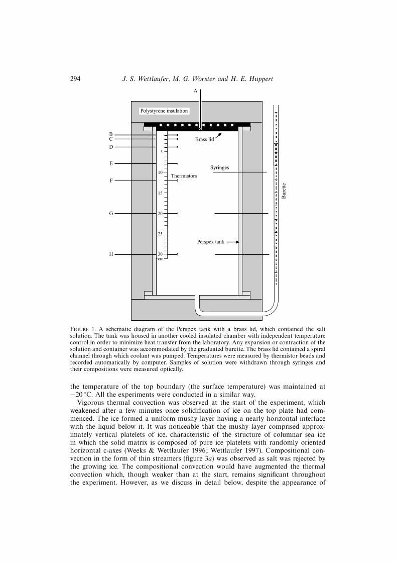
cooled and solidified from above. The apparatus consisted of a Perspex tank, withwalls 11 mm thick, of dimensions 20 × 20 × 37.6 cm with a brass lid as depicted infigure 1. The lid had a double-spiral channel within it through which was pumpedcooled ethylene glycol (anti-freeze). A thermistor, marked ‘A’, was embedded in thelid close to its contact with the liquid or mushy layer. The temperature of the coolantwas continually adjusted in order to achieve and maintain the lid at a constanttemperature. All the other walls of the tank were insulated with 5 cm thick expandedpolystyrene and the whole apparatus was placed in a chamber with independenttemperature control, thereby suppressing heat gains from the laboratory. The depthof the mushy layer was measured with a millimetre scale fixed to the side of the tank.Seven thermistors, marked ‘B’ to ‘H’, were placed at 1, 2, 4, 8, 12, 20 and 30 cm fromthe upper boundary, at least 5 cm away from any side wall. The tank was airtightand a tube led from a hole in its side near the base to allow for any expansion ofthe solution as it cooled and solidified. The tube led to a graduated burette so thatthe amount of expansion could be recorded as a function of time. This provided theprimary measurement from which the volume of ice grown was determined.
Before an experiment began the solution in the tank was cooled to a uniformtemperature of approximately −2 ◦C. This was the starting temperature for all theexperiments except two in which the concentration of the solution was only 1 wt%or 2 wt% NaCl. In these cases, the initial temperature of the solution was set towithin 1 ◦C above the relevant liquidus temperature (figure 2). An experiment wasstarted by allowing the pre-cooled refrigerant to circulate through the top plate.During the experiment, the thermistors were automatically monitored by a computer.Periodically, the depth of the mushy layer, the level of liquid in the burette and theconcentration of samples withdrawn at 10 cm, 20 cm and 30 cm below the cooledplate were recorded simultaneously.
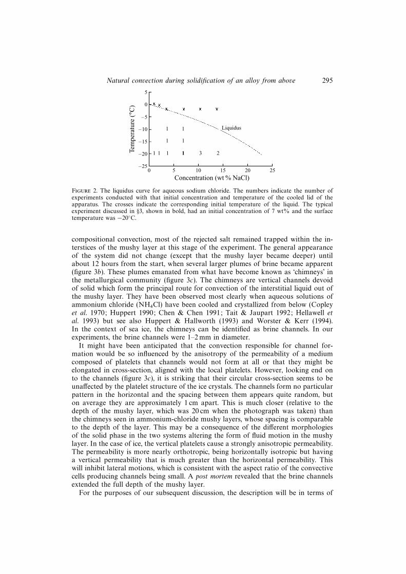
We report here on thirteen experiments with initial concentrations ranging from 1to 14 wt% NaCl and top-plate temperatures ranging between −10 ◦C and −20 ◦C.The initial conditions of the various experiments are shown in figure 2.
3. Results from a particular experimentBefore describing the suite of experiments in generality, we present in detail the
observations made and data collected from a particular experiment using an aqueoussolution of 7 wt% NaCl. The initial temperature of the solution was −1.84 ◦C and
294 J. S. Wettlaufer, M. G. Worster and H. E. Huppert
Syringes
G
H
D
BC
E
F
A
Bur
ette
Brass lid
Thermistors
Perspex tank
cm
5
10
15
20
25
30
Polystyrene insulation
Figure 1. A schematic diagram of the Perspex tank with a brass lid, which contained the saltsolution. The tank was housed in another cooled insulated chamber with independent temperaturecontrol in order to minimize heat transfer from the laboratory. Any expansion or contraction of thesolution and container was accommodated by the graduated burette. The brass lid contained a spiralchannel through which coolant was pumped. Temperatures were measured by thermistor beads andrecorded automatically by computer. Samples of solution were withdrawn through syringes andtheir compositions were measured optically.
the temperature of the top boundary (the surface temperature) was maintained at−20 ◦C. All the experiments were conducted in a similar way.
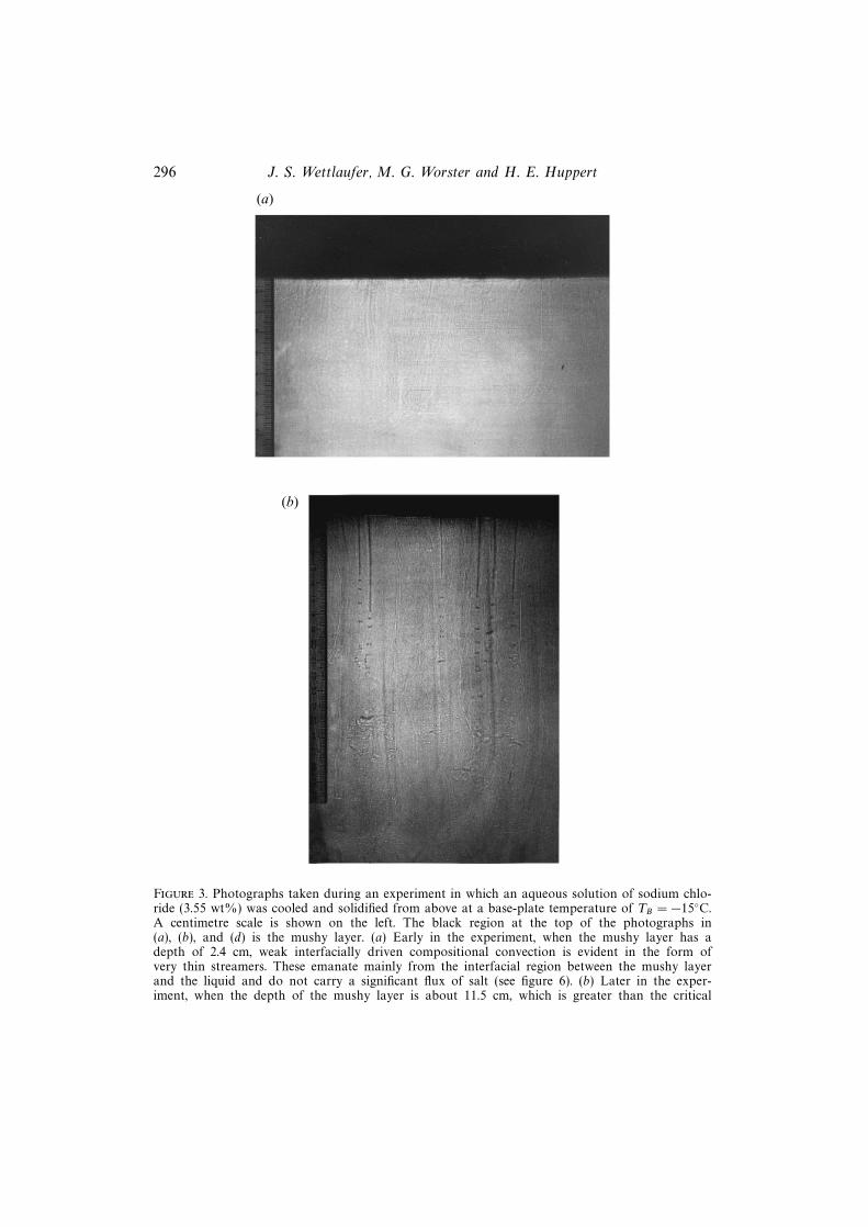
Vigorous thermal convection was observed at the start of the experiment, whichweakened after a few minutes once solidification of ice on the top plate had com-menced. The ice formed a uniform mushy layer having a nearly horizontal interfacewith the liquid below it. It was noticeable that the mushy layer comprised approx-imately vertical platelets of ice, characteristic of the structure of columnar sea icein which the solid matrix is composed of pure ice platelets with randomly orientedhorizontal c-axes (Weeks & Wettlaufer 1996; Wettlaufer 1997). Compositional con-vection in the form of thin streamers (figure 3a) was observed as salt was rejected bythe growing ice. The compositional convection would have augmented the thermalconvection which, though weaker than at the start, remains significant throughoutthe experiment. However, as we discuss in detail below, despite the appearance of
Natural convection during solidification of an alloy from above 295
0 5 10 15 20 25
Concentration (wt % NaCl)
11
1 1
1 1 1 1 3 2
Liquidus
5
0
–5
–10
–15
–20
–25
Tem
pera
ture
(°C
)
Figure 2. The liquidus curve for aqueous sodium chloride. The numbers indicate the number ofexperiments conducted with that initial concentration and temperature of the cooled lid of theapparatus. The crosses indicate the corresponding initial temperature of the liquid. The typicalexperiment discussed in §3, shown in bold, had an initial concentration of 7 wt% and the surfacetemperature was −20◦C.
compositional convection, most of the rejected salt remained trapped within the in-terstices of the mushy layer at this stage of the experiment. The general appearanceof the system did not change (except that the mushy layer became deeper) untilabout 12 hours from the start, when several larger plumes of brine became apparent(figure 3b). These plumes emanated from what have become known as ‘chimneys’ inthe metallurgical community (figure 3c). The chimneys are vertical channels devoidof solid which form the principal route for convection of the interstitial liquid out ofthe mushy layer. They have been observed most clearly when aqueous solutions ofammonium chloride (NH4Cl) have been cooled and crystallized from below (Copleyet al. 1970; Huppert 1990; Chen & Chen 1991; Tait & Jaupart 1992; Hellawell etal. 1993) but see also Huppert & Hallworth (1993) and Worster & Kerr (1994).In the context of sea ice, the chimneys can be identified as brine channels. In ourexperiments, the brine channels were 1–2 mm in diameter.
It might have been anticipated that the convection responsible for channel for-mation would be so influenced by the anisotropy of the permeability of a mediumcomposed of platelets that channels would not form at all or that they might beelongated in cross-section, aligned with the local platelets. However, looking end onto the channels (figure 3c), it is striking that their circular cross-section seems to beunaffected by the platelet structure of the ice crystals. The channels form no particularpattern in the horizontal and the spacing between them appears quite random, buton average they are approximately 1 cm apart. This is much closer (relative to thedepth of the mushy layer, which was 20 cm when the photograph was taken) thanthe chimneys seen in ammonium-chloride mushy layers, whose spacing is comparableto the depth of the layer. This may be a consequence of the different morphologiesof the solid phase in the two systems altering the form of fluid motion in the mushylayer. In the case of ice, the vertical platelets cause a strongly anisotropic permeability.The permeability is more nearly orthotropic, being horizontally isotropic but havinga vertical permeability that is much greater than the horizontal permeability. Thiswill inhibit lateral motions, which is consistent with the aspect ratio of the convectivecells producing channels being small. A post mortem revealed that the brine channelsextended the full depth of the mushy layer.
For the purposes of our subsequent discussion, the description will be in terms of
296 J. S. Wettlaufer, M. G. Worster and H. E. Huppert
(a)
(b)
Figure 3. Photographs taken during an experiment in which an aqueous solution of sodium chlo-ride (3.55 wt%) was cooled and solidified from above at a base-plate temperature of TB = −15◦C.A centimetre scale is shown on the left. The black region at the top of the photographs in(a), (b), and (d) is the mushy layer. (a) Early in the experiment, when the mushy layer has adepth of 2.4 cm, weak interfacially driven compositional convection is evident in the form ofvery thin streamers. These emanate mainly from the interfacial region between the mushy layerand the liquid and do not carry a significant flux of salt (see figure 6). (b) Later in the exper-iment, when the depth of the mushy layer is about 11.5 cm, which is greater than the critical
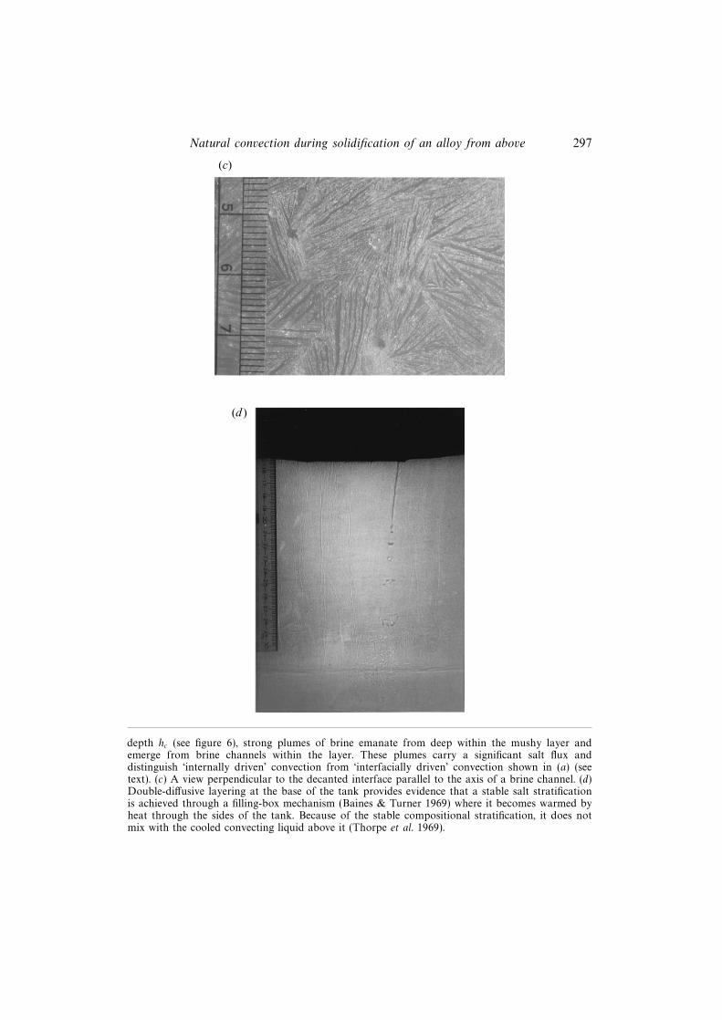
Natural convection during solidification of an alloy from above 297
(c)
(d )
depth hc (see figure 6), strong plumes of brine emanate from deep within the mushy layer andemerge from brine channels within the layer. These plumes carry a significant salt flux anddistinguish ‘internally driven’ convection from ‘interfacially driven’ convection shown in (a) (seetext). (c) A view perpendicular to the decanted interface parallel to the axis of a brine channel. (d)Double-diffusive layering at the base of the tank provides evidence that a stable salt stratificationis achieved through a filling-box mechanism (Baines & Turner 1969) where it becomes warmed byheat through the sides of the tank. Because of the stable compositional stratification, it does notmix with the cooled convecting liquid above it (Thorpe et al. 1969).
298 J. S. Wettlaufer, M. G. Worster and H. E. Huppert
Mushylayer
Compositionalconvection frominterface
Thermal convectionfrom interface
Salty plumesfrom mushylayer
Liquidregion
Cold plate
Figure 4. A schematic diagram indicating the three types of convection that occur in the ex-perimental system. Both small-scale compositional convection (depicted by small round arrows)and large-scale thermal convection (depicted by larger round arrows) originate from the interfacialregion between the mushy layer and the liquid region and keep the liquid well mixed. The initialsmall-scale compositional convection does not carry much salt and the concentration of the liquidregion remains constant to within the resolution of our measurements. After some time into anexperiment additional compostional convection (depicted by large vertical arrows) emerges in theform of plumes from the interior of the mushy layer and is replaced by a slow return flow of fresherliquid from below. This convection carries much more salt so, once it occurs, the composition of theliquid region evolves in time. It is likely that the plumes, which mix less well than the small-scaleconvection from the interface, are reponsible for setting up the weak compositional gradient at thebase of the tank that allows double-diffusive layers to form there (see figure 3d).
just two types of convection, as illustrated in figure 4. Convection is driven in theliquid region as a result of the density difference between the liquid near the mush–liquid interface and the liquid in the fully liquid region. This density difference is duepartly to a temperature difference and partly to a compositional difference. The latterwould be predicted to be zero in a theory that assumed thermodynamic equilibrium atthe mush–liquid interface and also assumed the interface to be planar. It is non-zeroonce either non-equilbrium effects are taken into account or it is appreciated thatcompositional convection can arise from the tips of the crystals in the neighbourhoodof the interface, in other words that the ‘interface’ is a region of finite size (Worster& Kerr 1994). We shall refer to the thermal and compositional convection drivenfrom the interfacial region as ‘interfacially driven’ convection. The second type ofconvection to which we shall refer is that emanating from the interior of the mushy
Natural convection during solidification of an alloy from above 299
0
–5
–10
–20
–15
0 100 200 300 400 500
E F G H
D
A
B
CTe
mpe
ratu
re
t (min)
Figure 5. The temperatures recorded by the thermistors as function of time. Note that thethermistors all record the same temperature while they are in the liquid region but record lowertemperatures once they are engulfed by the advancing mushy layer.
layer. We refer to this type of convection as ‘internally driven’ convection. It is drivenprimarily by compositional density gradients which dominate those caused by thethermal field within the mushy layer.
The primary data recorded from this experiment are shown in figures 5–9. Infigure 5, the temperature traces from all eight thermistors are shown. It can be seenthat the temperature of the cold upper boundary (thermistor A) dropped quicklyto −20 ◦C and was constant thereafter. Apart from minor fluctuations, the otherthermistors recorded the same (slowly decreasing) temperature while they were inthe liquid region but the traces peel off to lower values as each thermistor becameengulfed by the mushy layer. The temperature at the lowermost thermistor (H)increased slightly above the general temperature of the liquid region at late stagesin an experiment. This may be due to dense saline fluid ponding at the base ofthe tank by the filling-box mechanism (Baines & Turner 1969) where it becomeswarmed by heat from the laboratory. Although heated, it is too saline to mix withthe cooled convecting liquid above it. Indeed, there is some evidence of compositionalstratification near the base of the tank from the presence of double-diffusive layeringthere (figure 3d), probably caused by heat transfer through the sides of the tank actingon a stable compositional stratification (Thorpe, Hutt & Soulsby 1969).
In figure 6 we show the measured concentrations in the liquid region as functionsof time (figure 6a) and of the depth of the mushy layer (figure 6b). The compositionalstratification mentioned above was too weak to be resolved by the refractometer usedto determine the concentration. So, to within our experimental error, the compositionof the liquid region was uniform. It is clear that the concentration remained constantin time until after about 200 minutes, when the mushy layer was about 5 cm deep,as indicated by the hand-drawn curves in figure 6. In other words, essentially all thesalt rejected by the growing ice initially remained trapped within the interstices of themushy layer. This phase of the evolution corresponds to the form of compositionalconvection evident in figure 3(a). Our interpretation is that this weak convectionoriginates from the mush–liquid interfacial region where the interstitial concentrationis close to the far-field concentration in the liquid region. Only after the mushy layerhad grown to some depth hc, which we shall call the ‘critical depth’, was there asignificant flux of brine out of the mushy layer into the liquid beneath. The increasedbrine flux appears to be associated with the form of convection shown in figure 3(b),in which plumes of dense salty fluid emerge from deep within the mushy layer. The
300 J. S. Wettlaufer, M. G. Worster and H. E. Huppert
(b)
0 2 4 6 8 10 12 14
h (cm)
8.5
8.0
7.5
7.0
6.50 400 800 1200 1600 2000
10 h 30 h
(a)
C(wt % NaCl)
t (min)hc
Figure 6. (a) The concentration of the liquid region and (b) the depth of the mushy layer asfunctions of time. The concentration intially remains constant indicating that the salt rejected bythe growing ice remains trapped within the mushy layer. Once the depth of the mushy layer exceedsa critical value hc, salt is convected out of the mushy layer and causes the concentration of theliquid region to increase. The solid curves are hand-drawn to fit the data.
–2
–3
–4
–5
Tl (°C)
10 h 20 h0 500 1000 1500
t (min)
Figure 7. The temperature of the liquid region as a function of time. The crosses show theexperimental data while the four curves show the predictions of a mathematical model withdifferent values of the kinetic coefficient G and the heat-flux coefficient λ: – – – –, G = ∞, λ = 0.056;— — —, G = ∞, λ = 0.12; ——–, G = 4× 10⁻⁴, λ = 0.056, – · – · – · –, G = 2.2× 10⁻⁴, λ = 0.056.
initiation of a significant brine flux from the mushy layer only after the mushy layerhas achieved a certain depth is a central observation of this study, which we examinefurther in the following Sections.
It is helpful in understanding the consequences of the expulsion of interstitial brinefrom the mushy layer to compare and contrast the observations made using the presentsystem with the results of previous studies in which there was no compositionalconvection. In a series of papers, Kerr et al. (1990a,b) developed mathematicalmodels of binary alloys cooled from above which released a buoyant residual as theysolidified. The residual liquid remained in the mushy layer and did not contribute toany convection. The models take account of heat conduction and latent heat releasewithin the mushy layer and of the heat flux due to thermal convection in the liquidregion. Kerr et al. (1990a, b) computed results in very close agreement with theirexperimental data, so we use the models here with confidence that any discrepanciesbetween their predictions and our data are indicative of the influence of compositionalconvection.
In figure 7 we show the measured temperature of the liquid region as a function of
Natural convection during solidification of an alloy from above 301
0
–2
–4
–6
–8
Tl (°C)
6.5 7.0 7.5 8.0 8.5 9.0
C (wt % NaCl)
Liquidus
Figure 8. The trajectory of the temperature and concentration of the liquid region as they evolve intime. In the early stage of the experiment, thermal convection cools the liquid region to temperaturesclose to the liquidus temperature. Despite the small-scale compositional convection the compositionof the liquid region remains almost constant. Once compositional convection from the interior ofthe mushy layer begins, the concentration of the liquid region increases. The continuing thermalconvection keeps the temperature of the liquid close to the evolving liquidus temperature.
time and compare the data with four theoretical predictions. There are two parametersin the theory that may be influenced by the compositional field. One is a coefficientλ appearing in the relationship
Nu ≡ FT (H − h)k(Ti − Tl)
= 24/3λRa1/3 (3.1)
between the Nusselt number Nu for thermal convection in the liquid region and theRayleigh number
Ra =(ρi − ρl)g(H − h)3
µκ, (3.2)
where FT is the convective heat flux from the liquid region, Ti and ρi are thetemperature and density of the liquid at the mush–liquid interface, Tl and ρl are thetemperature and density of the fully liquid region, g is the acceleration due to gravity,H − h is the depth of the liquid region, and µ, k and κ are the dynamic viscosity,thermal conductivity and thermal diffusivity of the liquid. The other parameteris a kinetic coefficient G which determines the degree of interfacial undercoolingvia the relationship
h = G [TL(Cl)− Ti] , (3.3)
where TL(Cl) is the liquidus temperature of the liquid region and the dot denotesdifferentiation with respect to time (Kerr et al. 1990b). Note that when the kineticcoefficient is large Ti ≈ TL(Cl), which is the usual approximation of interfacial equi-librium. The first theoretical curve in figure 7 (shown with a short-dashed line) isthe prediction made assuming interfacial equilibrium (effectively infinite kinetic co-efficient G) and the same value of λ (namely 0.056) used by Kerr et al. (1990a).As explained by Kerr et al. (1990b), interfacial undercooling can be significant, andthey measured a value for G of 2.2 × 10⁻⁴ cm s−1 ◦C−1 for ice growing from amixture of water and isopropanol. This same value of G is used in the predictionshown with a dash-dot curve in figure 7. It is possible to achieve a better fit to thedata at early times by choosing a value of G = 4 × 10⁻⁴ cm s−1 ◦C−1, as shownby the solid curve in figure 7. A different value of G may be justified simply by
302 J. S. Wettlaufer, M. G. Worster and H. E. Huppert
t (min)
8
6
4
2
0
h (cm)
100 200 300 400 500
(a)
t (min)
20
5
0
h (cm)
500 1000
(b)
1500 2000
15
10
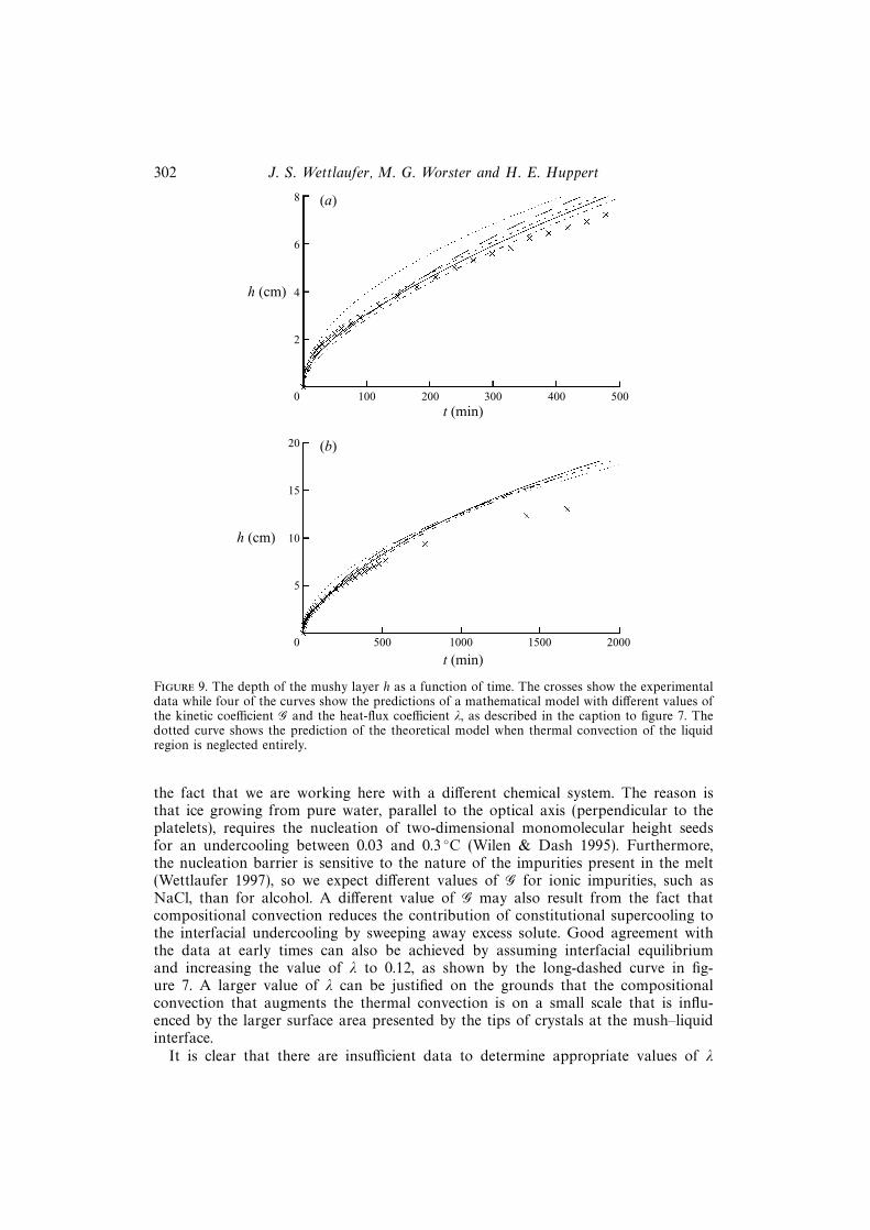
Figure 9. The depth of the mushy layer h as a function of time. The crosses show the experimentaldata while four of the curves show the predictions of a mathematical model with different values ofthe kinetic coefficient G and the heat-flux coefficient λ, as described in the caption to figure 7. Thedotted curve shows the prediction of the theoretical model when thermal convection of the liquidregion is neglected entirely.
the fact that we are working here with a different chemical system. The reason isthat ice growing from pure water, parallel to the optical axis (perpendicular to theplatelets), requires the nucleation of two-dimensional monomolecular height seedsfor an undercooling between 0.03 and 0.3 ◦C (Wilen & Dash 1995). Furthermore,the nucleation barrier is sensitive to the nature of the impurities present in the melt(Wettlaufer 1997), so we expect different values of G for ionic impurities, such asNaCl, than for alcohol. A different value of G may also result from the fact thatcompositional convection reduces the contribution of constitutional supercooling tothe interfacial undercooling by sweeping away excess solute. Good agreement withthe data at early times can also be achieved by assuming interfacial equilibriumand increasing the value of λ to 0.12, as shown by the long-dashed curve in fig-ure 7. A larger value of λ can be justified on the grounds that the compositionalconvection that augments the thermal convection is on a small scale that is influ-enced by the larger surface area presented by the tips of crystals at the mush–liquidinterface.
It is clear that there are insufficient data to determine appropriate values of λ
Natural convection during solidification of an alloy from above 303
400
300
200
100
0 400 800 1200 1600 2000
t (min)
Ve (cl)
10 h 30 h
Figure 10. The volume of fluid Ve in the graduated burette (expansion tube) as a function of timeduring the experiment.
and G with any certainty in the present system. However, it is the nature of thedisagreement between theory and experiment rather than any agreement that is ofprimary interest here. It is noticeable that none of the theoretical curves predict thesteady decline in the temperature at late times. This contrast between theory andexperiment highlights a consequence of compositional convection from the interiorof the mushy layer. As the concentration of the liquid region increases (as shownin figure 6) its liquidus temperature decreases. In particular, the temperature at themush–liquid interface decreases, which drives further thermal convection and coolsthe liquid region. Indeed, we see in figure 8 that the thermal convection is sufficientlystrong to keep the liquid region close to its liquidus temperature as it evolves in time.This evolution of the concentration field is not taken into account in the theoreticalpredictions displayed in figure 7.
A further influence of the expelled brine can be deduced from figure 9, which showsthe measured depth of the mushy layer as a function of time and four theoretical curvesusing the parameter values described above. Additionally, a theoretical prediction isshown in which the convective heat flux from the liquid region has artificially beenset to zero. It is first worth noting that the range of values of λ and G used in tryingto fit the temperature data makes little difference to the prediction of the growthof the mushy layer but that the thermal convection, though apparently weak, has ameasureable influence on the growth. The mushy layer starts to grow more slowlythan predicted by the theory after about 200 minutes. This is likely to be an indirectconsequence of the brine expulsion which begins at about 200 minutes, as shown infigure 6. As we shall see below, the expulsion of brine causes the solid fraction of themushy layer to increase. The associated increase in the amount of latent heat neededto be removed retards the growth of the mushy layer. The slower growth at late timesmay additionally be caused by some heat gains from the laboratory, which have adirect effect on thermal convection.
The last of the primary measurements made in our experiments was the volume ofliquid in the expansion tube, shown as a function of time in figure 10. The expansionis due primarily to the increase in specific volume that occurs as water freezes to formice. Roughly speaking, therefore, the volume of expansion Ve is proportional to thetotal volume of ice grown. However, great care is needed in order to interpret thesedata adequately, since Ve is also affected significantly by the change in the densityof the liquid with both temperature T and concentration C and the change in the
304 J. S. Wettlaufer, M. G. Worster and H. E. Huppert
1.028
1.027
1.026
1.025
1.024
1.023
1.106
1.104
1.102
1.100
1.098
1.096
Den
sity
(N
aCl)
(g
cm–
3 )
Den
sity
(N
aNO
3) (
g cm
–3 )
–5
(a)
0 5 10 15 20
Temperature (°C)
8
6
4
2
0
–2
–4
Ve (cl)
0 5 10 15 20
T (°C)
(b)
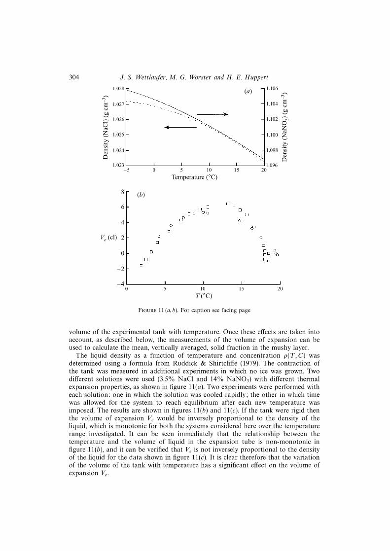
Figure 11 (a, b). For caption see facing page
volume of the experimental tank with temperature. Once these effects are taken intoaccount, as described below, the measurements of the volume of expansion can beused to calculate the mean, vertically averaged, solid fraction in the mushy layer.
The liquid density as a function of temperature and concentration ρ(T ,C) wasdetermined using a formula from Ruddick & Shirtcliffe (1979). The contraction ofthe tank was measured in additional experiments in which no ice was grown. Twodifferent solutions were used (3.5% NaCl and 14% NaNO3) with different thermalexpansion properties, as shown in figure 11(a). Two experiments were performed witheach solution: one in which the solution was cooled rapidly; the other in which timewas allowed for the system to reach equilibrium after each new temperature wasimposed. The results are shown in figures 11(b) and 11(c). If the tank were rigid thenthe volume of expansion Ve would be inversely proportional to the density of theliquid, which is monotonic for both the systems considered here over the temperaturerange investigated. It can be seen immediately that the relationship between thetemperature and the volume of liquid in the expansion tube is non-monotonic infigure 11(b), and it can be verified that Ve is not inversely proportional to the densityof the liquid for the data shown in figure 11(c). It is clear therefore that the variationof the volume of the tank with temperature has a significant effect on the volume ofexpansion Ve.
Natural convection during solidification of an alloy from above 305
60
50
40
30
20
10
0
–10
(d )1.0010
1.0000
1.9990
1.9980
1.9970
1.9960
Ve (cl)
T (°C)–5 0 5 10 15 20
VV0
(c)
–25 –20 –15 –10 –5 0 5
T –T0 (°C)
Figure 11. (a) The density of aqueous solutions of sodium nitrate (14 wt% NaNO3) and sodiumchloride (3.5 wt% NaCl) as functions of temperature. These solutions were used in additionalexperiments designed to determine the expansion properties of the experimental apparatus. Thevolume of fluid in the expansion tube is shown as a function of temperature during experiments inwhich (b) aqueous solutions of sodium chloride and (c) aqueous solutions of sodium nitrate werecooled without the formation of ice. The squares show the results obtained when the solutionswere cooled rapidly. The circles show the results obtained when time was left for the apparatus toslowly relax to each new temperature. Part (d) shows the volume of the experimental tank relativeto its initial value as a function of temperature. The line shows the best-fit linear relationship (3.5)through the data.
When no ice is grown, the volume of the tank V (T ) can be calculated by massconservation, which gives
V (T )
V0
=ρ0
ρ(T )
(1− Ve
V0
), (3.4)
where ρ(T ) is the known density of the liquid as a function of its temperature T and ρ0
and V0 are the initial density of the liquid and volume of the tank respectively. In thisformula, we have assumed that the liquid in the burette is at room temperature andhence retains its initial density. Since the burette contains only a small volume relativeto the volume of the tank, any error in this approximation is correspondingly small.
306 J. S. Wettlaufer, M. G. Worster and H. E. Huppert
0.8
0.7
0.6
0.5
φ
0 400 800 1200 1600 2000
t (min)
Figure 12. The mean solid fraction of the mushy layer as a function of time calculated from a massbalance (φm, equation (3.7), ×) and from a solute balance (φc, equation (3.9), �). The solid curve ishand drawn to fit the data for φc.
Figure 11(d) shows that all four experiments give essentially the same relationshipbetween the volume of the tank and the temperature, which is well approximated bythe linear expression
V = V0 [1− γ(T − T0)] , (3.5)
with γ ≈ 1.86× 10⁻⁴ ◦C−1.In the main experiments in which ice was grown, we estimate the mean, vertically
averaged, solid fraction of the mushy layer as follows. We assume that the mushylayer has a solid fraction φ that is uniform with depth and that the solid phasehas uniform density ρs. We estimate the density of the liquid in the mushy layer asρm = ρ(Tm, Cm), where Tm = 0.5[TL(Cl) + TB] = TL(Cm) and TL(C) is the liquidustemperature at concentration C (figure 2). Mass conservation for the whole system isexpressed by
where ρl = ρ(Tl, Cl) and Tl and Cl are the measured values of the temperature andconcentration of the liquid region. The mean solid fraction calculated from expression(3.7) is shown by the crosses in figure 12.
An alternative method for determining the mean solid fraction is via the equation
expressing conservation of solute (cf. expressions given by Tait & Jaupart 1992 andby Huppert & Hallworth 1993). This equation can be rearranged to give
φ =ρeCeVe + ρlClV − ρ0C0V0 + (ρmCm − ρlCl)hAm
ρmCmhAm≡ φc. (3.9)
The value of the mean solid fraction estimated in this way is shown by the opensquares in figure 12. The fact that the two estimates for φ agree shows consistencybetween the measurements of the volume of expansion and the measurements ofconcentration, and gives us confidence in the estimation of the solid fraction.
Natural convection during solidification of an alloy from above 307
It should be noted that at early times both the numerator and denominator aresmall in expressions (3.7) and (3.9), which makes the calculation of solid fraction verysensitive to experimental error for those times. This is consistent with the fact that itis at early times that there is the greatest discrepancy between the two estimates of themean solid fraction. It is tempting to conclude that the initial increase in φm, while φcis constant, is due to the nucleation barrier parallel to the horizontal c-axes causingdisequilibrium in the interior of the mushy layer (Wettlaufer 1997; Wilen & Dash1995). Such an effect would be seen in φm but, since it involves no transfer of soluteout of the mushy layer, would not be seen in φc. Although we cannot be sufficientlyconfident in these early-time measurements to draw such a firm conclusion, for thereasons mentioned above, we believe that the idea warrants future study.
The data presented in figure 12 show that the solid fraction of the mushy layerincreases monotonically with time. There is a sharp rise in the rate of increase afterabout 200 minutes at the same time when, as shown in figure 6(a), a significant saltflux out of the mushy layer commenced. We interpret this as indicating that as brineexits the mushy layer it is replenished by relatively fresh water from which more icecan be solidified.
4. Variations with external conditionsThe experimental procedure described in the previous Sections was repeated for
solutions of different initial concentrations C0 and for different surface temperaturesTB . We begin here by showing the overall trends in the evolution of the system asthese parameters vary.
Figure 13(a) shows how the depth of the mushy layer h grew as a function of timein three experiments in which the initial concentration C0 was 7 wt% and TB varied.As expected, we see that the growth is more rapid when the upper boundary is colder.We shall refer to the temperature difference TL(C0) − TB as the ‘thermal driving’ ofthe system. Greater thermal driving results in faster growth of the depth of the mushylayer.
Greater thermal driving (for a given concentration) also results in the mushy layerhaving a larger solid fraction, as shown in figure 13(b). This has a significant influenceon the solute flux that can convect out of the mushy layer, since the greater solidfraction provides a greater resistance to the flow of interstitial liquid. For example, wesee from figure 13(c) that the critical depth hc before a significant solute flux beganwas largest in the experiment with the coldest surface temperature. This is a strikingobservation given that the compositional density difference across the mushy layeravailable to drive convection is greatest in this case. However, the greater resistance toflow associated with the larger solid fraction has the dominant influence and retardsthe release of interstitial brine.
Once the critical depth has been reached, the subsequent flux of solute was greatestin the system with the greatest thermal driving, as can be seen in figure 13(d). By thisstage in the evolution of these experiments, the three systems had approximately thesame solid fraction for a given depth of mushy layer (see §5), so the strength of thethermal driving alone determined the solute flux.
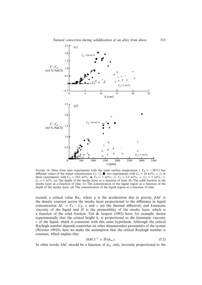
These trends are emphasized further in figure 14, where the evolutions of allexperiments with the same value of the surface temperature TB = −20◦C but differentinitial concentrations are shown. Since the liquidus temperature TL(C) decreases withconcentration, the thermal driving TL(C0)−TB also decreases. The growth is therefore
308 J. S. Wettlaufer, M. G. Worster and H. E. Huppert
(a)
12
8
4
h (cm)
(b)
T B= –20 °C
T B= –15 °C
T B= –10 °C
T B= –20 °C
T B= –15 °C
T B= –10 °C
20 h 40 h
0t (min)
500 1000 1500 2000 2500
20 h 40 h
0.8
0.7
0.6
0.4
0.3
0.5
φm
0t (min)
500 1000 1500 2000 2500
Figure 13 (a, b). For caption see facing page.
slower for larger values of C0, as shown in figure 14(a) and the solid fraction is lower,as shown in figure 14(b).
In figure 14(c) we see again that the permeability has a greater influence on therelease of solute from the mushy layer than does the thermal driving. At low initialconcentrations the thermal driving is large but the solid fraction is also large so theresistance to flow is large. The latter effect is dominant and we see that the criticaldepth of the mushy layer decreases as the initial concentration increases.
Figure 14(d) shows that the solute flux increases as the initial concentration in-creases, even though the thermal driving decreases. This is in contrast with figure 13(d)which shows the solute flux increasing with the thermal driving. The results shown infigure 14(d) display the dominance of the solid fraction in determining the composi-tional convection since the solid fraction is large (the permeability is low) when theinitial concentration is small.
We have seen qualitatively how the critical height hc varies with the imposed condi-tions of the experiment. In the next Section we explore these variations quantitativelyin an attempt to determine a general criterion for the abrupt onset of internally drivenconvection.
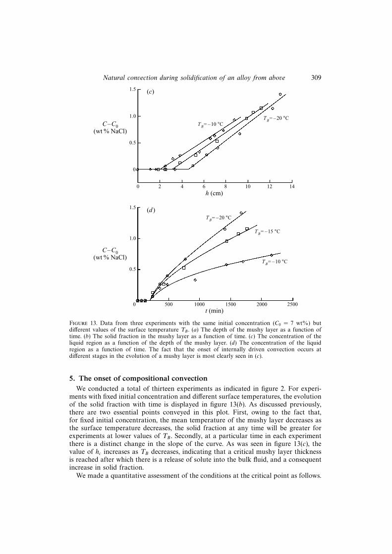
Natural convection during solidification of an alloy from above 309
1.5
0
(c)
(d )
T B= –20 °CT B= –10 °C
T B= –20 °C
T B= –15 °C
T B= –10 °C
0t (min)
500 1000 1500 2000 2500
0
1.0
0.5
2 4 6 8 10 12 14h (cm)
C–C0(wt % NaCl)
1.5
1.0
0.5
C–C0(wt % NaCl)
Figure 13. Data from three experiments with the same initial concentration (C0 = 7 wt%) butdifferent values of the surface temperature TB . (a) The depth of the mushy layer as a function oftime. (b) The solid fraction in the mushy layer as a function of time. (c) The concentration of theliquid region as a function of the depth of the mushy layer. (d) The concentration of the liquidregion as a function of time. The fact that the onset of internally driven convection occurs atdifferent stages in the evolution of a mushy layer is most clearly seen in (c).
5. The onset of compositional convectionWe conducted a total of thirteen experiments as indicated in figure 2. For experi-
ments with fixed initial concentration and different surface temperatures, the evolutionof the solid fraction with time is displayed in figure 13(b). As discussed previously,there are two essential points conveyed in this plot. First, owing to the fact that,for fixed initial concentration, the mean temperature of the mushy layer decreases asthe surface temperature decreases, the solid fraction at any time will be greater forexperiments at lower values of TB . Secondly, at a particular time in each experimentthere is a distinct change in the slope of the curve. As was seen in figure 13(c), thevalue of hc increases as TB decreases, indicating that a critical mushy layer thicknessis reached after which there is a release of solute into the bulk fluid, and a consequentincrease in solid fraction.
We made a quantitative assessment of the conditions at the critical point as follows.
310 J. S. Wettlaufer, M. G. Worster and H. E. Huppert
25
5
(a)
20
15
10
h (cm)
0 500 1000 1500 2000 2500 3000 3500
t (min)
C0=1 wt %
C0=14 wt %
1.0 (b)
0.8
0.4
φm 0.6
0 500 1000 1500 2000 2500 3000 3500
t (min)
C0=1 wt %
C0=14 wt %
0.2
Figure 14 (a, b). For caption see facing page.
From graphs such as 13(c) we fitted a low-order polynomial (for h(C)) to the datacorresponding to liquid concentrations greater than the initial concentration C0, i.e.beyond the critical point. The polynomial was used to extrapolate backwards todetermine the value of h = hc, when C = C0. The data for φm and h were then usedto determine φmc = φm(hc), the value of the mean solid fraction at the critical point.
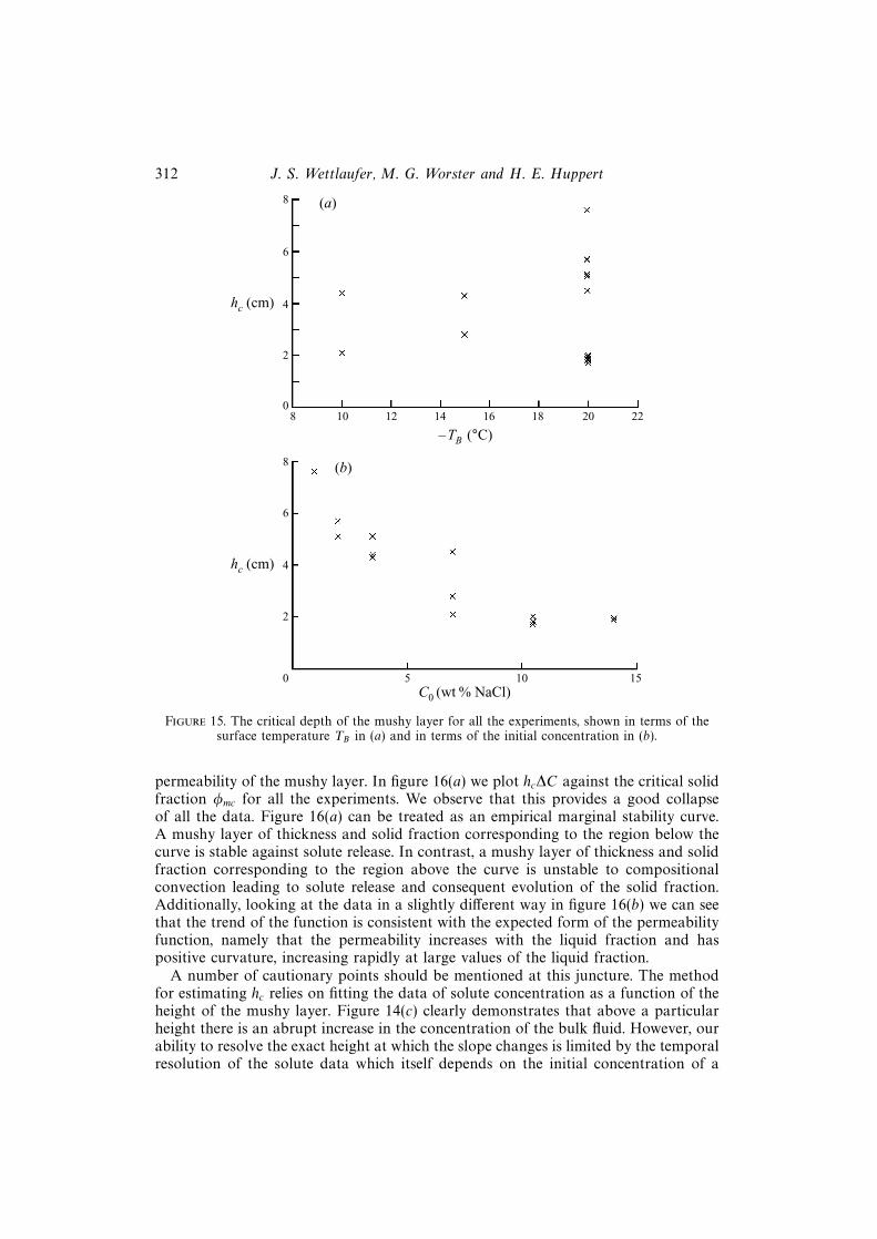
The critical height hc varies considerably with the conditions of the experiment, TBand C0, as shown in figures 15(a) and 15(b). Although we can determine from thesegraphs the general trends that hc increases as TB decreases at fixed C0 and that hcdecreases as C0 increases at fixed TB , the data generally display a striking lack ofcorrelation. A reasonable collapse of all the data can, however, be achieved using thefollowing physical hypothesis.
Theoretical stability analyses of growing mushy layers (Fowler 1985; Worster 1992b;Chen, Lu & Yang 1994) have shown that the buoyant interstitial fluid can remainmotionless until a porous-medium Rayleigh number
Ra =gβ∆CΠ(φm)h
κν(5.1)
Natural convection during solidification of an alloy from above 311
(c)
h (cm)5 10 15 2520
C0=1 wt %
C0=14 wt %
2.5
0
2.0
1.5
1.0
0.5
0
–0.5
C–C0(wt % NaCl)
(d )
C0=1 wt %
C0=14 wt %
2.5
2.0
1.5
1.0
0.5
500 1000 1500 2000 2500 3000 3500t (min)
0
C–C0(wt % NaCl)
Figure 14. Data from nine experiments with the same surface temperature ( TB = −20◦C) butdifferent values of the initial concentration C0: �, �, two experiments with C0 = 14 wt%; ◦, �, •,three experiments with C0 = 10.5 wt%; �, C0 = 7 wt%; 4, C0 = 3.5 wt%; +, C0 = 2 wt%; ×,C0 = 1 wt%. (a) The depth of the mushy layer as a function of time. (b) The solid fraction in themushy layer as a function of time. (c) The concentration of the liquid region as a function of thedepth of the mushy layer. (d) The concentration of the liquid region as a function of time.
exceeds a critical value Rac, where g is the acceleration due to gravity, β∆C isthe density contrast across the mushy layer proportional to the difference in liquidconcentration ∆C = C0 − CB , κ and ν are the thermal diffusivity and kinematicviscosity of the liquid and Π is the permeability of the mushy layer, which isa function of the solid fraction. Tait & Jaupart (1992) have, for example, shownexperimentally that the critical height hc is proportional to the kinematic viscosityν of the liquid, which is consistent with this same hypothesis. Although the criticalRayleigh number depends somewhat on other dimensionless parameters of the system(Worster 1992b), here we make the assumption that the critical Rayleigh number isconstant, which implies that
(h∆C)−1 ∝ Π(φmc). (5.2)
In other words, h∆C should be a function of φmc only, inversely proportional to the
312 J. S. Wettlaufer, M. G. Worster and H. E. Huppert
(a)
(b)
8 10 12 14 16 18 20 22
8
6
4
2
0
hc (cm)
8
6
4
2
0
hc (cm)
5 10 15C0 (wt % NaCl)
–TB (°C)
Figure 15. The critical depth of the mushy layer for all the experiments, shown in terms of thesurface temperature TB in (a) and in terms of the initial concentration in (b).
permeability of the mushy layer. In figure 16(a) we plot hc∆C against the critical solidfraction φmc for all the experiments. We observe that this provides a good collapseof all the data. Figure 16(a) can be treated as an empirical marginal stability curve.A mushy layer of thickness and solid fraction corresponding to the region below thecurve is stable against solute release. In contrast, a mushy layer of thickness and solidfraction corresponding to the region above the curve is unstable to compositionalconvection leading to solute release and consequent evolution of the solid fraction.Additionally, looking at the data in a slightly different way in figure 16(b) we can seethat the trend of the function is consistent with the expected form of the permeabilityfunction, namely that the permeability increases with the liquid fraction and haspositive curvature, increasing rapidly at large values of the liquid fraction.
A number of cautionary points should be mentioned at this juncture. The methodfor estimating hc relies on fitting the data of solute concentration as a function of theheight of the mushy layer. Figure 14(c) clearly demonstrates that above a particularheight there is an abrupt increase in the concentration of the bulk fluid. However, ourability to resolve the exact height at which the slope changes is limited by the temporalresolution of the solute data which itself depends on the initial concentration of a
Natural convection during solidification of an alloy from above 313
200
150
100
50
0 0.2 0.4 0.6 0.8 1.0
(a)
(b)
hc(CB–C0)
Internally drivencompositional convection
Interfacially drivenconvection
0.06
φmc
0.04
0.02
0 0.1 0.2 0.3 0.4 0.5 0.6 0.7
1–φmc
1
hc (CB–C0)
Figure 16. (a) The critical conditions for the onset of internally driven compositional convection.The crosses show the data for when the brine flux began in each experiment. When the conditionsof the mushy layer lie below the marginal curve drawn through the data, most of the salt rejectedby the growing ice remains trapped in the mushy layer. Once the conditions of the mushy layer lieabove the marginal curve then brine is convected out of the mushy layer. (b) Here we display thesame data in a different way by plotting (h∆C)−1, which is proportional to the permeability, againstthe mean liquid fraction (1− φmc). This shows that the trend of the observations is consistent withthe expected form of the permeability function, namely that the permeability increases with theliquid fraction and has positive curvature, increasing rapidly at large values of the liquid fraction.
given experiment (i.e. for low initial concentrations, we are in a position of measuringsmall variations in a small quantity). We believe that the actual solute release beginsat a height that is a little lower than that which we estimate. Furthermore, since weuse hc to estimate φmc, we believe that the critical value of the solid fraction is anupper bound. Therefore, the empirical marginal stability curve represents an upperbound for both hc∆C and φmc.
A final curiosity is shown in figure 17, where we plot the solid fraction as afunction of the depth of the mushy layer for experiments with an initial concentrationC0 = 7 wt% and three different surface temperatures. It appears that once significantcompositional convection from the mushy layer has begun (i.e. once the critical depthhc has been exceeded) the data conform to a single curve. Similar results were found
314 J. S. Wettlaufer, M. G. Worster and H. E. Huppert
0.8
0.7
0.5
φm
0.6
0
0.4
0.32 4 6 8 10 12 14
h (cm)
Figure 17. The mean solid fraction of the mushy layer as a function of its depth for threeexperiments with the same initial concentration (C0 = 7 wt%) but different values of the surfacetemperature TB . The data appear to collapse to a single curve once internally driven convection hasbegun.
for the experiments having C0 = 3.5 wt%; the curves have a similar shape, but thesolid fraction is generally higher. In other words, the solid fraction appears to begiven by φ = φ(h, C0) independent of the surface temperature. The implication is thatonce h > hc in a given system, one need only know the depth of the mushy layer inorder to determine its solid fraction. This observation merits further investigation.
6. Discussion and conclusionsWe have conducted a systematic experimental study of the freezing of ice from salt
water cooled from above. The ice forms a mushy layer whose interstices are filledwith liquid enriched by the salt rejected by the growing ice. Although dense, the saltyliquid remains within the mushy layer initially but, once the depth of the layer exceedsa critical value, compositional convection of brine into the underlying liquid regioncan commence.
The critical depth is larger when the surface temperature is colder for given initialconcentration and is smaller when the initial concentration is larger for given surfacetemperature. In general, the critical depth is consistent with the hypothesis that it isdetermined by the critical conditions for compositional convection within the porousmushy layer.
The compositional convection out of the mushy layer allows fresher water toenter it, which promotes the further growth of ice within it and so increases thesolid fraction. The present study provides the first laboratory measurements of theevolution of the solid fraction of sea ice. We have shown how the solid fractionincreases with time, most markedly once the critical depth has been exceeded.
It is generally held that the brine flux from growing sea ice increases as the surfacetemperature decreases (gets colder). The accepted reason for this is simply that coldersurface temperatures increase the rate of growth of ice and hence the rate of rejectionof brine. However, as we have seen, the rejected brine can remain trapped withinthe mushy layer (sea-ice layer) and, indeed, that it remains trapped for longer andthe critical depth is greater when the surface temperature is colder. Once the critical
Natural convection during solidification of an alloy from above 315
depth is exceeded then the brine flux is indeed greater when the surface temperature iscolder but this is because the contrast in the liquid concentration is then greater andprovides a correspondingly greater density contrast to drive compositional convection.
We have found, in experiments with similar initial concentrations, that, once thecritical depth has been exceeded, the solid fraction is a function of the depth ofthe mushy layer alone, independent of the surface temperature. Colder surface tem-peratures increase the rate of growth of the depth h of the mushy layer and alsoincrease the rate of expulsion of brine thus increasing the rate of growth of the meansolid fraction φ, apparently in a way that keeps φ = φ(h). We cannot yet offer anexplanation for this but, if more generally true than within the constraints of ourexperimental procedure, this fact has extremely important implications. In particular,scattering theories developed specifically for the remote sensing of thin sea ice (Wine-brenner et al. 1992) show that the volume scattering (as distinct from the surfacescattering) is principally determined by the brine fraction (liquid fraction) of the ice.If indeed φ = φ(h) alone then measurements of brine fraction would simultaneouslydetermine the depth of the sea ice cover and hence the total solidified volume. Thisis a key observation for the monitoring of sea-ice climatology. Further implicationsof this work, including how our finding of an abrupt onset of brine flux affects thethermohaline structure in the Arctic Ocean, are discussed in Wettlaufer et al. (1997).It is possible that the overall brine flux is enhanced by the interaction between flow ofthe oceanic boundary layer and that within the sea ice. This is the subject of currentstudy and has yet to be quantified.
It is our eventual goal to be able to construct a predictive theoretical modelof the formation of sea ice. We have shown that existing models are adequate tomake predictions in the early stages of its formation before a significant flux ofbrine from the mushy layer occurs. However, it remains to model the compositionalconvection within the mushy layer sufficiently to predict the salt flux once the criticalconditions have been exceeded. The results of the experiments reported here shouldguide the development of future theories and provide a benchmark against which totest them.
We thank M. A. Hallworth for considerable help with the experiments and R. C.Kerr for useful comments on an earlier version of the manuscript. The work waspartially supported by ONR N00014-94-1-0120, NSF OPP9523513 and NERC.
REFERENCES
Aagaard, K. & Carmack, E. 1994 A synthesis of Arctic Ocean circulation. In The Polar Regionsand Their Role in Shaping the Global Environment (ed. O. M. Johannessen, R. D. Muench &J. E. Overland), pp. 5–20, Geophysical Monograph 85. American Geophysical Union.
Baines, W. D. & Turner, J. S. 1969 Turbulent buoyant convection from a source in a confinedregion. J. Fluid Mech. 37, 51–80.
Bennington, K. O. 1963 Some crystal growth features of sea ice. J. Glaciol. 4, 669–688.
Chen, C. F. & Chen, F. 1991 Experimental study of directional solidification of aqueous ammoniumchloride solution. J. Fluid Mech. 227, 567–586.
Chen, F., Lu, J. W. & Yand, T. L. 1994 Convective instability in ammonium chloride solutiondirectionally solidified from below. J. Fluid Mech. 276 163–187.
Copley, S. M., Giamei, A. F., Johnson, S. M. & Hornbecker, M. F. 1970 The origin of freckles inbinary alloys. Metall. Trans. A1, 2193–2204.
Eide, L. I. & Martin, S. 1975 The formation of brine drainage features in young sea ice. J. Glaciol.14, 137–154.
Fowler, A. C. 1985 The formation of freckles in binary alloys. IMA J. Appl. Maths 35, 159–174.
316 J. S. Wettlaufer, M. G. Worster and H. E. Huppert
Gill, A. E. 1973 Circulation and bottom water production in the Weddell Sea. Deep-Sea Res. 20,111–140.
Hellawell, A., Sarazin, J. R. & Steube, R. S. 1993 Channel convection in partly solidified systems.Phil. Trans. R. Soc. Lond. A 345, 507–544.
Huppert, H. E. 1990 The fluid dynamics of solidification. J. Fluid Mech. 212, 209–240.
Huppert, H. E. & Hallworth, M. A. 1993 Solidification of NH4Cl and NH4Br from aqueoussolutions contaminated by CuSO4: the extinction of chimneys. J. Cryst. Growth 130, 495–506.
Huppert, H. E. & Worster, M. G. 1985 Dynamic solidification of a binary melt. Nature 314,703–707.
Kerr, R. C., Woods, A. W., Worster, M. G. & Huppert, H. E. 1990a Solidification of an alloycooled from above. Part 1. Equilibrium growth. J. Fluid Mech. 216, 323–342.
Kerr, R. C., Woods, A. W., Worster, M. G. & Huppert, H. E. 1990b Solidification of an alloycooled from above. Part 2. Non-equilibrium interfacial kinetics. J. Fluid Mech. 217, 331–348.
Lake, R. A. & Lewis, E. L. 1970 Salt rejection by sea ice during growth. J. Geophys. Res. 75,583–597.
Morison, J., McPhee, M., Muench, R. et al.: THE LEADEX GROUP 1993 The LeadEx experi-ment. Eos, Trans. AGU 74, 393–397.
Malmgren, F. 1927 On the properties of sea ice. In The Norwegian Polar Expedition ‘Maud,’1918-1925, Scientific Results, vol. 1a(5), pp. 1–67.
Peixoto, J. P. & Oort, A. H. 1992 Physics of Climate. American Institute of Physics.
Ruddick, B. R. & Shirtcliffe, T. G. L. 1979 Data for double-diffusers: physical properties ofaqueous salt–sugar solutions. Deep-Sea Res. 26A, 775–787.
Tait, S. & Jaupart, C. 1992 Compositional convection in a reactive crystalline mush and meltdifferentiation. J. Geophys. Res. 97, 6735–6756.
Thorpe, S. A., Hutt, P. K. & Soulsby, R. 1969 The effect of horizontal gradients on thermohalineconvection. J. Fluid Mech. 46, 299–319.
Turner, J. S. 1979 Buoyancy Effects in Fluids. Cambridge University Press.
Weeks, W. F. 1997 Growth conditions and the structure and properties of sea ice. In IAPSOAdvanced Study Institute–Summer School: Physics of Ice–Covered Seas (ed. M. Lepparanta).University of Helsinki.
Weeks, W. F. & Wettlaufer, J. S. 1996 Crystal orientations in floating ice sheets, In The JohannesWeertman Symposium (ed. R. J. Arsenault et al.), pp. 337–350. The Minerals, Metals & MaterialsSociety.
Wettlaufer, J. S. 1997 Introduction to crystallization phenomena in sea ice. In IAPSO AdvancedStudy Institute–Summer School: Physics of Ice–Covered Seas (ed. M. Lepparanta). Universityof Helsinki.
Wettlaufer, J. S., Worster, M. G. & Huppert, H. E. 1997 The phase evolution of young sea ice.Geophys. Res. Lett. 23, 1251–1254.
Wilen, L. A. & Dash, J. G. 1995 Giant facets at ice grain boundary grooves. Science 270, 1184–1186.
Williams, K. L., Garrison, G. R. & Mourad, P. D. 1992 Experimental examination of growingand newly submerged sea ice including acoustic probing of the skeletal layer. J. Acoust. Soc.Am. 92, 2075–2092.
Winebrenner, D. P., Bredow, J., Fung, A. K. et al. 1992 Microwave sea ice signature modeling.In Microwave Remote Sensing of Sea Ice (ed. F. Carsey), pp. 137–75. Geophysical Monograph68, American Geophysical Union.
Worster, M. G. 1992a The dynamics of mushy layers. In Interactive Dynamics of Convection andSolidification (ed. S. H. Davis, H. E. Huppert, U. Muller & M. G. Worster). NATO ASI E219,pp. 113–138. Kluwer.
Worster, M. G. 1992b Instabilities of the liquid and mushy regions during solidification of alloys.J. Fluid Mech. 237, 649–669.
Worster, M. G. & Kerr, R. C. 1994 The transient behaviour of alloys solidified from below priorto the formation of chimneys. J. Fluid Mech. 269, 23–44.