NAVAL POSTGRADUATE SCHOOL - apps.dtic.mil · location methods are explored to quantify the effects...

NAVAL POSTGRADUATE

SCHOOL MONTEREY, CALIFORNIA

THESIS

Approved for public release; distribution is unlimited

PASSIVE COHERENT DETECTION AND TARGET LOCATION WITH MULTIPLE NON-COOPERATIVE

TRANSMITTERS

by

Qinling Jeanette Olivia Tan

June 2015

Thesis Advisor: David C. Jenn Co-Advisor: Edward Fisher

THIS PAGE INTENTIONALLY LEFT BLANK

i

REPORT DOCUMENTATION PAGE Form Approved OMB No. 0704–0188Public reporting burden for this collection of information is estimated to average 1 hour per response, including the time for reviewing instruction, searching existing data sources, gathering and maintaining the data needed, and completing and reviewing the collection of information. Send comments regarding this burden estimate or any other aspect of this collection of information, including suggestions for reducing this burden, to Washington headquarters Services, Directorate for Information Operations and Reports, 1215 Jefferson Davis Highway, Suite 1204, Arlington, VA 22202-4302, and to the Office of Management and Budget, Paperwork Reduction Project (0704-0188) Washington, DC 20503. 1. AGENCY USE ONLY (Leave blank) 2. REPORT DATE

June 2015 3. REPORT TYPE AND DATESCOVERED

Master’s Thesis 4. TITLE AND SUBTITLEPASSIVE COHERENT DETECTION AND TARGET LOCATION WITH MULTIPLE NON-COOPERATIVE TRANSMITTERS

5. FUNDING NUMBERS

6. AUTHOR(S) Qinling Jeanette Olivia Tan7. PERFORMING ORGANIZATION NAME(S) AND ADDRESS(ES)

Naval Postgraduate School Monterey, CA 93943-5000

8. PERFORMINGORGANIZATION REPORT NUMBER

9. SPONSORING /MONITORING AGENCY NAME(S) AND ADDRESS(ES)N/A

10. SPONSORING/MONITORING AGENCY REPORT NUMBER

11. SUPPLEMENTARY NOTES The views expressed in this thesis are those of the author and do not reflect the officialpolicy or position of the Department of Defense or the U.S. Government. IRB Protocol number ____N/A____.

12a. DISTRIBUTION / AVAILABILITY STATEMENT Approved for public release; distribution is unlimited

12b. DISTRIBUTION CODE

13. ABSTRACT (maximum 200 words)

Passive bistatic radars (PBR) and passive multistatic radars (PMR) use opportunistic transmitters to detect and locate targets. In this thesis, a maritime scenario was modeled with merchant vessels serving as multiple non-cooperative opportunistic transmitters while a frigate warship equipped with Electronic Warfare (EW) and Direction Finding (DF) receivers takes on the role of the receiver in a PBR/PMR configuration. The targets are assumed to be the generic Formidable-class frigate.

A MATLAB model is developed to simulate the operating environment and passive detection and location process. Detection coverage is investigated to propose optimal PBR/PMR configurations and geometry, while elliptical and hyperbolic target location methods are explored to quantify the effects of PBR/PMR parameters and geometry on target estimated location uncertainty.

14. SUBJECT TERMSbistatic, multistatic, target detection, target location, passive coherent detection, non-cooperative transmitters, opportunistic transmitters, hitchhiker radar, forward-scattering, back-scattering, error ellipse, uncertainty ellipse

15. NUMBER OFPAGES

169 16. PRICE CODE

17. SECURITYCLASSIFICATION OF REPORT

Unclassified

18. SECURITYCLASSIFICATION OF THIS PAGE

Unclassified

19. SECURITYCLASSIFICATION OF ABSTRACT

Unclassified

20. LIMITATIONOF ABSTRACT

UU NSN 7540–01-280-5500 Standard Form 298 (Rev. 2–89)

Prescribed by ANSI Std. 239–18

ii


iii

Approved for public release; distribution is unlimited

PASSIVE COHERENT DETECTION AND TARGET LOCATION WITH MULTIPLE NON-COOPERATIVE TRANSMITTERS

Qinling Jeanette Olivia Tan Civilian, DSO National Laboratories, Singapore B.Eng, National University of Singapore, 2010

Submitted in partial fulfillment of the requirements for the degree of

MASTER OF SCIENCE IN INFORMATION WARFARE SYSTEMS ENGINEERING

from the

NAVAL POSTGRADUATE SCHOOL June 2015

Author: Qinling Jeanette Olivia Tan

Approved by: David C. Jenn Thesis Advisor

Edward Fisher Co-Advisor

Dan Boger Chair, Department of Information Sciences Department

iv


v

ABSTRACT

Passive bistatic radar (PBR) and passive multistatic radar (PMR) use opportunistic

transmitters to detect and locate targets. In this thesis, a maritime scenario was modeled

with merchant vessels serving as multiple non-cooperative opportunistic transmitters,

while a frigate warship equipped with Electronic Warfare (EW) and Direction

Finding (DF) receivers takes on the role of the receiver in a PBR/PMR configuration. The

targets are assumed to be the generic Formidable-class frigate.

A MATLAB model is developed to simulate the operating environment and

passive detection and location process. Detection coverage is investigated to propose

optimal PBR/PMR configurations and geometry, while elliptical and hyperbolic target

location methods are explored to quantify the effects of PBR/PMR parameters and

geometry on target estimated location uncertainty.

vi


vii

TABLE OF CONTENTS

I. INTRODUCTION........................................................................................................1 A. OVERVIEW .....................................................................................................1 B. HISTORY .........................................................................................................3

1. First Resurgence...................................................................................3 2. Second Resurgence...............................................................................4 3. Third Resurgence .................................................................................4

C. RECENT DEVELOPMENTS IN BISTATIC AND MULTISTATIC RADAR .............................................................................................................6

D. THESIS OBJECTIVE .....................................................................................8 E. THESIS CHAPTER OUTLINE ...................................................................10

II. BISTATIC RADAR THEORY .................................................................................11 A. DEFINITION .................................................................................................11 B. RANGE EQUATION ....................................................................................11 C. TARGET LOCATION EQUATIONS .........................................................16

1. Bistatic Radar Trigonometry ............................................................16 2. Least-Squares Intersection of Lines .................................................19 3. Hyperbolic Target Location ..............................................................22

D. MEASUREMENT AND LOCATION ERRORS .......................................25 1. Time Delay (Range) Measurements .................................................26 2. Angle Measurements .........................................................................26 3. Transmitter and Receiver Position Accuracy .................................27 4. Receiver-to-Target Range Error ......................................................27

E. ERROR ELLIPSE PARAMETERS ............................................................28

III. MATLAB AND FEKO MODELING ......................................................................33 A. PROBLEM SETUP .......................................................................................33 B. FEKO MODEL ..............................................................................................34 C. MATLAB MODEL ........................................................................................37

1. Detection Coverage Model 1 .............................................................38 2. Detection Coverage Model 2 .............................................................39 3. Simulation Duration and Accuracy Trade-off ................................41 4. Target Location Model ......................................................................44

D. MODEL VERIFICATION ...........................................................................44

IV. SIMULATION RESULTS ........................................................................................49 A. DETECTION COVERAGE .........................................................................49

1. Bistatic RCS ........................................................................................49 2. General Observations ........................................................................50

3. Vary Number of Transmitters ..........................................................52

4. Vary Transmitter Range ...................................................................54

5. Vary Transmitter-Target-Receiver Geometry ................................56 6. Target Path Detection ........................................................................60

B. TARGET LOCATION ESTIMATION .......................................................62

viii

1. General Observations ........................................................................62 2. Error Ellipse of Target Position Estimate .......................................64

V. CONCLUSION ..........................................................................................................73 A. SUMMARY OF FINDINGS .........................................................................73

1. Findings for Detection Coverage ......................................................73 2. Findings for Target Location ............................................................74

B. FUTURE WORK ...........................................................................................75

APPENDIX A. DERIVATION OF ERROR ELLIPSE PARAMETERS FROM BIVARIATE NORMAL DISTRIBUTION .............................................................77

APPENDIX B. SPECIFICATION SHEET FOR MANTADIGITAL RADAR BY KELVIN HUGHES ....................................................................................................87

APPENDIX C. SPECIFICATION SHEET FOR TELEDYNE DEFENCE QR026 EW RECEIVER .........................................................................................................89

APPENDIX D. SPECIFICATION SHEET FOR POYNTING DEFENCE DF-A0062 DF RECEIVER ..........................................................................................................91

APPENDIX E. DETECTION COVERAGE PLOTS FOR TARGET PLANE IN S-BAND ..........................................................................................................................93

APPENDIX F. DETECTION COVERAGE RESULTS ....................................................99

F.1 VARY NUMBER OF TRANSMITTERS .........................................................99 F.2 VARY TRANSMITTER RANGE ...................................................................109 F.3 VARY TRANSMITTER-TARGET-RECEIVER GEOMETRY .................113 F.4 RANDOMLY DISTRIBUTED TRANSMITTERS .......................................117

APPENDIX G. TARGET PATH DETECTION RESULTS............................................123

APPENDIX H. TARGET LOCATION RESULTS ..........................................................127

LIST OF REFERENCES ....................................................................................................141

INITIAL DISTRIBUTION LIST .......................................................................................145

ix

LIST OF FIGURES

Bistatic radar geometry. .....................................................................................3 Figure 1. Pictorial representation of the PBR setup. After [4]. .........................................9 Figure 2. Cassini oval for c b where 1 2b rr . ..............................................................13 Figure 3. Bistatic radar geometry for converting North-referenced coordinates into Figure 4.

polar coordinates. After [2]. .............................................................................13

Ovals of Cassini, contours of constant SNR (dB), with 430K L . After Figure 5.[2]. ....................................................................................................................14

Timing sequence diagram for direct and indirect method for calculating Figure 6.range sum ( )T RR R . From [2]. ......................................................................17

Reception of direct and reflected pulses. .........................................................18 Figure 7. Least-squares intersection of lines solution to three PBR case........................20 Figure 8. Perpendicular distance from a point to a line. From [32]. ...............................21 Figure 9.

Single PBR in multi-bistatic radar scenario. ....................................................23 Figure 10. Error ellipse parameters. ..................................................................................28 Figure 11. Chi-square probability density function with 2 degrees of freedom. The Figure 12.

area to the right of 2 critical value is . ......................................................30

Error ellipse rotation to achieve statistical independence. From [38]. ............31 Figure 13. Frigate FEKO model (top) and actual RSN Formidable-class frigate Figure 14.

(bottom; from [39]). Side-profile. ....................................................................35 Frigate FEKO model and coordinate system. ..................................................36 Figure 15. Frigate’s monostatic RCS (dBsm) (left) and bistatic RCS (dBsm) with Figure 16.

incident angle of 10° (right) at 3.05 GHz. .......................................................36 Frigate bistatic RCS (dBsm) with incident angle of 10° at 3.05 GHz. RCS Figure 17.

at 1° resolution (left) and 0.1° resolution (right). ............................................37 MATLAB Detection Coverage Model 1 flowchart. ........................................39 Figure 18. MATLAB Detection Coverage Model 2 flowchart .........................................40 Figure 19. Detection coverage of a 40 km × 40 km area of interest grid points at 1 km Figure 20.

resolution..........................................................................................................42

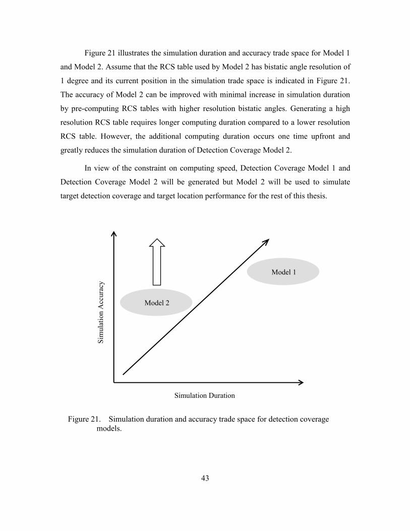
Simulation duration and accuracy trade space for detection coverage Figure 21.models. .............................................................................................................43

Detection coverage contours for constant RCS target. ....................................45 Figure 22. Target plate FEKO model. ...............................................................................46 Figure 23. Target plate S-Band azimuth RCS (dBsm) at φ=90° incidence. .....................46 Figure 24. Target bistatic RCS (dBsm) with incident angle 10° at 3.0 GHz (left) and Figure 25.

9.41 GHz. .........................................................................................................50 Target positions in forward-scattering and back-scattering configuration Figure 26.

on detection coverage plot. ..............................................................................51

Detection gaps and bearings extending from Tx-Rx baseline in detection Figure 27.coverage plot. ...................................................................................................52

Detection coverage plots at S-Band for with target plate at 0° orientation Figure 28.as the number of transmitters varies. ...............................................................53

x

Detection coverage plots at S-Band with target plate at 0° orientation as Figure 29.the transmitter range to receiver increases. ......................................................55

Detection coverage at S-Band for 4 Tx in receiver-centered geometry and Figure 30.target plate at 30° orientation. ..........................................................................57

Detection coverage at S-Band for 4 Tx in transmitter-clustered geometry Figure 31.and target plate at 30° orientation. ...................................................................57

Detection coverage at S-Band for 20 Tx randomly positioned around Rx at Figure 32.5–30 km range and target plate at 0° orientation. ............................................58

Detection coverage at S-Band for 20 Tx randomly positioned around Rx at Figure 33.5–30 km range and target plate at -90° orientation. .........................................59

Detection coverage at S-Band for 20 Tx randomly positioned around Rx at Figure 34.5–30 km range and target plate at 45° orientation. ..........................................60

Five target paths used to generate target path detection performance results.Figure 35...........................................................................................................................61

Detection coverage along target’s path at S-Band for 4 Tx (left) and 20 Tx Figure 36.(right). RCS extracted from pre-computed RCS table. ....................................61

Dilution of precision comparison between elliptical and hyperbolic Figure 37.methods using SNR-independent measurement errors. ...................................63

Target location errors using hyperbolic method (S-Band) with SNR-Figure 38.dependent measurement errors. .......................................................................64

Target position estimate scatter plot from elliptical method for target in Figure 39.Tx-Rx cluster. ..................................................................................................65

Target position estimate scatter plot from hyperbolic method for target in Figure 40.Tx-Rx cluster. ..................................................................................................66

Target position estimate scatter plot from elliptical method for target Figure 41.outside Tx-Rx cluster. ......................................................................................66

Target position estimate scatter plot from hyperbolic method for target Figure 42.outside Tx-Rx cluster. ......................................................................................67

Uncertainty area associated with position estimates from elliptical method Figure 43.for target in Tx-Rx cluster. ...............................................................................68

Uncertainty area associated with position estimates from elliptical method Figure 44.for target outside Tx-Rx cluster. ......................................................................68

Elliptical iso-contours of constant time delay measurements with Figure 45.transmitter and receiver at ellipse foci. ............................................................69

Uncertainty area associated with position estimates from hyperbolic Figure 46.method for target in Tx-Rx cluster. ..................................................................70

Uncertainty area associated with position estimates from hyperbolic Figure 47.method for target outside Tx-Rx cluster. .........................................................70

Hyperbolic target location estimate’s error ellipse at 50%, 70%, 90%, and Figure 48.99% confidence levels. ....................................................................................72

Joint Gaussian pdf surface and contours for various x , y , and xy values. Figure 49.After [38]. ........................................................................................................79

Eigenvectors 1 2, of a covariance matrix on an error ellipse. ...................80 Figure 50. Chi-square pdf for p degrees of freedom. ......................................................82 Figure 51.

xi

Chi-square pdf where the area to the right of the critical value is . .............83 Figure 52. Rotation of error ellipse principle axis. From [38]. .........................................84 Figure 53. Technical Specifications for MantaDigital Radar by Kelvin Hughes. From Figure 54.

[43]. ..................................................................................................................88 Technical Specifications for Teledyne Defence QR026 EW Receiver. Figure 55.

From [44]. ........................................................................................................90 Technical Specifications for Poynting Defence DF A0062 DF Receiver. Figure 56.

From [45]. ........................................................................................................91 Detection coverage (left) for Tx at [-5000, 0] and target plate at 0° Figure 57.

orientation with corresponding S-band bistatic RCS (right). ...........................93

Detection coverage (left) for Tx at [-5000, 0] and target plate at 0° Figure 58.orientation with corresponding S-band bistatic RCS (right). ...........................94


Detection coverage (left) for Tx at [-5000, 0] and target plate at -90° Figure 60.orientation with corresponding S-band bistatic RCS (right). ...........................95


Detection coverage (left) for Tx at [0, 5000] and target plate at 45° Figure 62.orientation with corresponding S-band bistatic RCS (right). ...........................96

Detection coverage (left) for Tx at [-5000,0] and target plate at -45° Figure 63.orientation with corresponding S-band bistatic RCS (right). ...........................96

Detection coverage (left) for Tx at [0, 5000] and target plane at -45° Figure 64.orientation with corresponding S-band bistatic RCS (right). ...........................97

Detection coverage at S-Band for 1 Tx at 5 km range and target at 0° Figure 65.orientation. .......................................................................................................99

Detection coverage at S-Band for 1 Tx at 5 km range and target at 90 Figure 66.orientation. .......................................................................................................99

Detection coverage at X-Band for 1 Tx at 5 km range and target at 0° Figure 67.orientation. .....................................................................................................100

Detection coverage at X-Band for 1 Tx at 5 km range and target at 90 Figure 68.orientation. .....................................................................................................100

Detection coverage at S-Band for 2 Tx at 5 km range and target at 0° Figure 69.orientation. .....................................................................................................101

Detection coverage at S-Band for 2 Tx at 5 km range and target at 90 Figure 70.orientation. .....................................................................................................101





xii



















Detection coverage at S-Band for 4 Tx in receiver-centered geometry and Figure 93.target at 0° orientation. ...................................................................................113

Detection coverage at S-Band for 4 Tx in receiver-centered geometry and Figure 94.target at -90° orientation. ...............................................................................113

Detection coverage at S-Band for 4 Tx in receiver-centered geometry and Figure 95.target at 45° orientation. .................................................................................114

Detection coverage at S-Band for 4 Tx in receiver-centered geometry and Figure 96.target at 30° orientation. .................................................................................114

xiii

Detection coverage at S-Band for 4 Tx in transmitter-clustered geometry Figure 97.and target at 0° orientation. ............................................................................115

Detection coverage at S-Band for 4 Tx in transmitter-clustered geometry Figure 98.and target at -90° orientation. ........................................................................115

Detection coverage at S-Band for 4 Tx in transmitter-clustered geometry Figure 99.and target at 45° orientation. ..........................................................................116

Detection coverage at S-Band for 4 Tx in transmitter-clustered geometry Figure 100.and target at 30° orientation. ..........................................................................116

Detection coverage at S-Band for 8 Tx randomly positioned around Rx at Figure 101.5–20 km range and target at 0° orientation. ...................................................117




Detection coverage at S-Band for 8 Tx randomly positioned around Rx at Figure 105.5–20 km range and target at -90° orientation. ...............................................119




Detection coverage at S-Band for 8 Tx randomly positioned around Rx at Figure 109.5–20 km range and target at 45° orientation. .................................................121




Detection coverage along target’s path (2 km resolution) at S-Band for 4 Figure 113.Tx. RCS computed by calling FEKO. ...........................................................123

SNR at receiver along target’s path (2 km resolution) at S-Band for 4 Tx. Figure 114.RCS computed by calling FEKO. ..................................................................123

Detection coverage along target’s path (100 m resolution) at S-Band for 4 Figure 115.Tx. RCS extracted from pre-computed RCS table.........................................124

SNR at receiver along target’s path (100 m resolution) at S-Band for 4 Tx. Figure 116.RCS extracted from pre-computed RCS table. ..............................................124

Detection coverage along target’s path (100 m resolution) at S-Band for 8 Figure 117.Tx randomly position. RCS extracted from pre-computed RCS table. .........125

SNR at receiver along target’s path (100 m resolution) at S-Band for 8 Tx Figure 118.randomly position. RCS extracted from pre-computed RCS table. ...............125

xiv

Target location errors using elliptical method (S-Band, 4 Tx at 5 km Figure 119.range) and SNR-independent measurement errors. .......................................127

Target location errors using hyperbolic method (S-Band, 4 Tx at 5 km Figure 120.range) and SNR-independent measurement errors. .......................................127

Target location errors using elliptical method (S-Band, 8 Tx at 5 km range) Figure 121.and SNR-independent measurement errors. ..................................................128






Target location errors using elliptical method (S-Band, 4 Tx clustered) and Figure 127.SNR-independent measurement errors. .........................................................131

Target location errors using hyperbolic method (S-Band, 4 Tx clustered) Figure 128.and SNR-independent measurement errors. ..................................................131

Target location errors using elliptical method (S-Band, 8 Tx clustered) and Figure 129.SNR-independent measurement errors. .........................................................132

Target location errors using hyperbolic method (S-Band, 8 Tx clustered) Figure 130.and SNR-independent measurement errors. ..................................................132

Target location errors using elliptical method (S-Band, 4 Tx at 5 km range) Figure 131.and SNR-dependent measurement errors.......................................................133

Target location errors using hyperbolic method (S-Band, 4 Tx at 5 km Figure 132.range) and SNR-dependent measurement errors. ..........................................133

Target location errors using elliptical method (S-Band, 8 Tx at 5 km range) Figure 133.and SNR-dependent measurement errors.......................................................134


Target location errors using elliptical method (S-Band, 4 Tx at 15 km Figure 135.range) and SNR-dependent measurement errors. ..........................................135


Target location errors using elliptical method (S-Band, 8 Tx at 15 km Figure 137.range) and SNR-dependent measurement errors. ..........................................136


Target location errors using elliptical method (S-Band, 8 Tx at random Figure 139.positions) and SNR-dependent measurement errors. .....................................137

Target location errors using hyperbolic method (S-Band, 8 Tx at random Figure 140.positions) and SNR-dependent measurement errors. .....................................137

xv

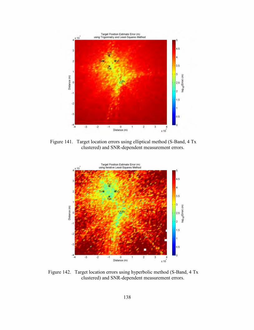
Target location errors using elliptical method (S-Band, 4 Tx clustered) and Figure 141.SNR-dependent measurement errors. ............................................................138

Target location errors using hyperbolic method (S-Band, 4 Tx clustered) Figure 142.and SNR-dependent measurement errors.......................................................138

Target location errors using elliptical method (S-Band, 8 Tx clustered) and Figure 143.SNR-dependent measurement errors. ............................................................139

Target location errors using hyperbolic method (S-Band, 8 Tx clustered) Figure 144.and SNR-dependent measurement errors.......................................................139

xvi


xvii

LIST OF TABLES

Table 1. Parameters of significant passive bistatic radar programs designed and tested for air surveillance. After [5]. ..................................................................5

Table 2. Signal parameters for typical passive radar illumination sources. From [23]. ....................................................................................................................7

Table 3. Target path information format in Excelsheet. ................................................38 Table 4. RCS table format in Excelsheet. ......................................................................41 Table 5. Percentage of grid points with SNR greater than 10 dB within a 10 km

radius centered at the receiver. Target orientation at 0°. .................................54 Table 6. Percentage of grid points with SNR greater than 10 dB within a 10 km

radius centered at the receiver. Target orientation at -90°. ..............................54 Table 7. Percentage of grid points with SNR greater than 10 dB within a 20 km

radius centered at the receiver. Target orientation at 0°. .................................56 Table 8. Chi-square distribution table ............................................................................83

xviii


xix

LIST OF ACRONYMS AND ABBREVIATIONS

AIS automatic identification system

AOA angle of arrival

ARM anti-radiation missile

BRRE bistatic radar range equation

CFAR constant false alarm rate

CMR civil marine radar

CST Computer Simulation Technology

DAB digital audio broadcasting

DF direction finding

DGPS Differential Global Positioning System

DOP dilution of precision

drms distance root mean square

DVB-T digital video broadcasting terrestrial

EA electronic attack

ESM electronic support measures

EW electronic warfare

FEKO field calculations for bodies with arbitrary surface (FEldberechnung für Körper mit beliebiger Oberfläche)

FFI The Norwegian Defence Research Establishment

(Forsvarets forskningsintitutt)

FM frequency modulation

FSR forward-scattering radar

GPS Global Positioning System

HF high frequency

ISAR inverse synthetic aperture radar

LOS line-of-sight

LPI low probability of intercept

MIMO multiple-input multiple-output

MTI moving target indicator

MWS Microwave Studio

xx

OODA observe–orient–decide–act

PBR passive bistatic radar

pdf probability density function

PMR passive multistatic radar

RAM radar-absorbent material

RCS radar cross section

rms root mean square

rss root-sum-squared

SAR synthetic aperture radar

SNR signal-to-noise ratio

STAP space time adaptive processing

TDOA time difference of arrival

UHF ultra-high frequency

USCG U.S. Coast Guard

UWB ultra-wideband

VHF very high frequency

xxi

ACKNOWLEDGMENTS

I would like to extend my deepest appreciation and gratitude to the following

people who have contributed one way or another in making this study possible.

Dr. David C. Jenn, thesis advisor, for his valuable support, advice, and guidance

leading to the completion of this thesis. His knowledge and experience helped me better

understand the issues at hand and overcome difficulties during the duration of this study.

Mr. Edward Fisher, thesis co-advisor, for his support and provisions rendered

during my course of study at NPS whilst allowing me the freedom to explore this thesis

topic.

DSO National Laboratories, for supporting my decision to pursue my master’s

education at NPS.

ME5 Chong Sze Sing, Republic of Singapore Navy (RSN), for the discussions

that led to a better understanding of the topic of using opportunistic transmitters for the

detection of maritime targets.

Lastly, I would like to express my immeasurable appreciation to my family and

friends for their understanding and unwavering support as I seek to further my studies.

xxii


1

I. INTRODUCTION

A. OVERVIEW

Since the concept of radar engineering was first demonstrated in 1904, progress in

radar technology has been driven by growing requirements for radar performance and

rapidly changing operating environment. A long detection range and wide coverage,

measurement accuracy, greater system capacity, and an ability to operate with the

presence of interference are some of the fundamental radar requirements that have been

established over the past few decades [1]. These radar performance characteristics—

together with the need to detect, separate, classify, locate, and track sources of emissions

in multi-target environments—triggered the development of passive radar detection and

location techniques.

The vast majority of today’s deployed radar systems are monostatic, that is, the

transmitting and receiving antennas are collocated. Despite the advancements in

antennas, transmitters, receivers, and processing technology, as well as passive radar

systems, conventional monostatic radar remains a double-edged sword—whereby it

detects targets, but radar transmission makes it vulnerable to detection—and may not be

the best option to address certain operational scenarios. A promising solution is to use

multiple radar transmitting and receiving sites to exploit spatial advantage for

coordinated target detection. Multi-site radars can be broadly classified into bistatic radar

and multistatic radar. Bistatic radar is a radar system where the transmitter and receiver

are located at different sites [2]. Similarly, a multistatic radar system utilizes multiple

spatially separated transmitter and receiver sites where the target information from all

receivers is fused [1]. Passive bistatic or multistatic radar capitalizes on transmitters of

opportunity to detect and locate sources of transmission or targets without deliberate

emissions. The illuminators are not limited to radar signals and include (but are not

limited to) analog TV, FM radio, digital video broadcasting terrestrial (DVB-T), digital

audio broadcasting (DAB), cellular network, WiFi, and Global Positioning System (GPS)

satellite signals [3].

2

In naval operations, targets employing low radar cross section (RCS) and radar-

absorbent material (RAM) design methods, coupled with the use of highly sensitive

electronic warfare (EW) receivers on warships, have changed the nature of the game.

Military ships are pressured to limit transmissions to avoid detection by highly sensitive

EW receivers. Furthermore, the use of low probability of intercept (LPI) radar in a

monostatic configuration results in weak returns from low-RCS targets, restricting

detection capability and compromising situational awareness. This thesis explores the use

of multiple pairs of passive bistatic radar (PBR) to detect low-RCS targets using

opportunistic transmissions as a possible solution and to validate the findings in [4].

Figure 1 shows the bistatic radar geometry for a PBR pair. The direct line-of-sight (LOS)

distance between the transmitter (Tx) and receiver (Rx) is known as the baseline and is

denoted by L . The distance between the transmitter and target is denoted as TR while

the distance between the receiver and the target is denoted as RR . The bistatic angle is

the angle subtended between transmitter, target, and receiver.

The proposed PBR approach offers potential advantage in the detection of

stealthy, low-RCS targets which are designed to minimize monostatic radar echoes. RCS

returns of stealthy ships vary with bistatic angle β and can be sufficiently large at certain

return directions. PBR capitalizes on this characteristic using opportunistic transmissions

to detect low-RCS targets. Being a passive system, PBR allows the receiver to remain

covert, making it more resilient to detection and electronic attack (EA)—in the form of

jamming and anti-radiation missiles (ARMs). The ability to leverage available

transmission and to detect targets passively also serves to enhance situational awareness,

thereby advancing one’s position in the observe–orient–decide–act (OODA) loop during

an operation [4]. It is also advantageous to use multiple transmitters at separate locations

for detection as it adds spatial diversity, which enhances detection accuracy and aids in

removing clutter, interference, and potential system errors. Lastly, the PBR system

proposed requires no additional equipment as all necessary hardware is currently

available on most naval ships.

3

Bistatic radar geometry. Figure 1.

B. HISTORY

The concept of Radio Detection and Ranging (RADAR) was first demonstrated in

1904 by German inventor Christian Hülsmeyer in a monostatic setup [5]. Following this,

radar experiments in the United States, the United Kingdom, France, Italy, Russia, and

Japan were carried out predominantly with bistatic radar operating in the forward-

scattering configuration [6]. However, the invention of the radar duplexer in 1936

addressed the issue of transmitter-receiver isolation and broadened the application of

single-site radar on aircraft, ships, and mobile ground units. By the end of World War II,

bistatic radar was displaced by monostatic radar, with the former experiencing periodic

resurgences [5].

1. First Resurgence

The 1950s saw renewed interest in bistatic radar with developments in missile and

satellite detection, location and tracking, semi-active homing missiles, hitchhiking, and

second-generation forward-scattering fences [2]. During this period, advancement in

Target (Tgt)

Bistatic Angle, β

Transmitter (Tx) Receiver (Rx)

Baseline, L

Direct path

RT RR

Illuminating Path

Target Echo Path

4

radar theory led to a better appreciation of concepts on match filtering, ambiguity

functions, statistical theories on detection, moving target indicator (MTI) radar, and

synthetic aperture radar (SAR) [7–9]. The term bistatic radar originated with K. M.

Siegel and R. E. Machol in 1952 [10].

2. Second Resurgence

The development of counter-measures to anti-radiation missiles (ARMs) and

emitter location-directed artillery in the 1970s resulted in the second resurgence in

bistatic radar. With a dual or multiple site configuration, the effectiveness of electronic

support measures (ESM) directed attacks can be reduced by locating the transmitter away

from the receiver or into a less vulnerable sanctuary [5]. The advent of digital processing

techniques during this period increased the processing capability in MTI operation modes

and allowed real-time airborne SAR mapping [7].

3. Third Resurgence

Research on bistatic space–time adaptive processing (STAP) to address moving

clutter and concepts to improve bistatic SAR images signaled the start of the third

resurgence. It was also during this period that passive bistatic radar surfaced as a possible

counter stealth technique. The idea for PBR is to utilize commercial broadcast signals in

bistatic or multistatic configurations to detect low-RCS targets [5]. Since then, several

PBR systems have been developed and evaluated for air surveillance. Some notable PBR

air surveillance systems are listed in Table 1.

5

Table 1. Parameters of significant passive bistatic radar programs designed and tested for air surveillance.* After [5].

System Silent SentryTM

TV-Based Bistatic

Radar (I)

TV-Based Bistatic

Radar (II)

FM Radio –Based

Bistatic Radar

Multistatic HDTV-Based

Radar

Developer

IBM, now Lockheed

Martin

Univ College London

DERA, United Kingdom NATO SAIC, U.S.

Army

Decade configuration 1980 – 2000 1980 1990 2000

2000

Transmitter operation

Multistatic: Rx: 1

Tx: up to 6 Bistatic

Bistatic Near-forward

scatter Bistatic

Multistatic: Rx: 4 Tx: 1

Baseline 100 km typical 12 km 150 km 50 km

10 km typical

Target

Aircraft Missile

launches

Aircraft

Aircraft

Aircraft

Aircraft below ~ 5000

ft

Target data

Range

Doppler Bearing

Range Bearing

Doppler Bearing

Range Doppler Bearing

Range

Doppler

Measured performance

RM = 100 km – 150 km

2-D tracks on A/C

3-D tracks on missile

launches

RM ~ 25 km Occasional

A/C detections, but

mostly negative

RM ~ 160 km Detections on

high and medium

altitude A/C but only 1/3

tracked

RM ~ 175 km Achieved with

innovative direct path excision

RM ~ 30 km Target location

via multi-lateration

Ghost excision via Doppler association

Status

Version 3 for sale to U.S. Government

for < 1 million dollars Work

continues

Program ended

Program ended

Program continuing

possible in a multistatic

mode

Test phase complete Awaiting

evaluation/ funding

* MR is the equivalent maximum monostatic range defined as 1/2max( )R T MR R R , where RR is the

receiver-to-target range and TR is the transmitter-to-target range.

6

C. RECENT DEVELOPMENTS IN BISTATIC AND MULTISTATIC RADAR

Despite research progress on improving the detection, classification, and location

performance of passive bistatic radar systems, their reliance on transmissions of

opportunity and the restricted geometry has limited their application. This fundamental

requirement continues to stimulate research and experimentation on opportunistic

illuminating sources, their optimum configuration, applicability, and performance in

various operational scenarios. As with all radar systems, improvement in interference and

clutter rejection, target detection, classification, and location and tracking accuracy are

current areas of interest in the field of passive bistatic radar and passive multistatic radar

(PMR). The recent research topics in bistatic and multistatic radar can be classified as

bistatic and multistatic system configuration, forward-scattering radar, and multiple-input

multiple-output (MIMO) radar.

When the concept of bistatic and multistatic radar was first introduced, dedicated

radar transmitters were used as transmission sources [11] before transmitters of

opportunity were employed as illuminating sources. Transmitters of opportunity in the

very high frequency (VHF) and ultra-high frequency (UHF) band, such as FM broadcast,

TV broadcast, DAB, DVB-T, and cellular network signals continue to be common

illuminating sources used in detecting airborne, land, and maritime targets [11–19].

Conversely, studies on the use of high frequency (HF) band signals as opportunistic

transmitters only started recently. HF signals present advantages of long range detection

and coverage, propagation beyond the radar horizon, and improved detection of stealth

targets, which enhances the PBR/PMR’s early warning capability [20, 21]. A list of

common transmission sources and their typical parameters are given in Table 2.

Apart from terrestrial sources of transmission, there has been recent interest in

using satellite transmissions to detect airborne targets. The SABER-DEMO platform

recently demonstrated its ability to detect aircraft passively using signal processing

techniques to process weak satellite sources of transmission [22].

7

Table 2. Signal parameters for typical passive radar illumination sources. From [23].

Transmission Frequency Modulation, Bandwidth t tPG

Power Density (Wm-2)

214

t tPGr

HF broadcast 10-30 MHz* DSB AM, 9 kHz 50 MW -67 to -53 dBW m-2 at r1

= 1000 km

VHF FM (analogue)

~100 MHz FM, 50 kHz 250 kW -57 dBW m-2 at r1 = 100 km

UHF TV (analogue) ~550 MHz

Vestigial-Sideband AM (vision); FM(sound),

5.5 MHz

1 MW -51 dBW m-2 at r1 = 100 km

Digital audio broadcast

~220 MHz digital, OFDM 220 kHz 10 kW -71 dBW m-2 at r1 = 100

km

Digital TV ~750 MHz digital, 6 MHz 8 kW -72 dBW m-2 at r1 = 100 km

Cellphone base station (GSM)

900 MHz, 1.8 GHz

GMSK, FDM/TDMA/FDD 200

kHz

100 W -81 dBW m-2 at r1 = 10 0km

Cellphone base station (3G) 2 GHz CDMA 5 MHz 100 W -81 dBW m-2 at r1 = 100

km *Appropriate frequency will depend on time of day.

Another topic of interest is the use of inverse synthetic aperture radar (ISAR)

processing techniques with forward-scattering radar (FSR) for target detection and

parameter extraction. FSR is the earliest form of bistatic radar where target detection

occurs at the transmitter to receiver baseline. The target’s radar cross section is enhanced

in the forward-scattering configuration due to Babinet’s principle [2]. Using the constant

false alarm rate (CFAR) approach, target detection and parameter extraction can be

accomplished in real time [24]. An experiment conducted at Forsvarets forskningsintitutt

(FFI) explores the difference in ISAR ship signatures in the forward and back-scattering

configurations. The results from the study show that forward-scattering returns produce

more accurate ISAR signatures than back-scattering returns as the RCS for forward-

scattering is usually stronger than back-scattering. The difference between forward and

back-scattering ISAR signatures can be fused to improve ship identification and

8

classification [25]. Apart from studies on FSR processing techniques to improve target

detection and extraction, considerable research has been conducted on ultra-wideband

(UWB) FSR for its ability to reduce sea clutter in maritime applications [26, 27].

Recent advances and interest in MIMO radar systems can be attributed to its

potential for detection and location of targets in bistatic or multistatic configurations.

Spatial diversity in MIMO radar systems exploits the differences in target cross section in

detecting and extracting target parameters such as angle of arrival (AOA) and Doppler

frequencies [28]. Furthermore, coherent processing in MIMO systems improves target

location accuracy [28, 29].

As with all studies in the radar domain, current bistatic and multistatic research

areas are motivated by the need to improve detection capability and measurement

accuracy while reducing or mitigating the effects of unwanted interference.

D. THESIS OBJECTIVE

The primary objectives of this thesis are as follows:

1. Generate a MATLAB model that computes a system’s detection performance given the target’s path.

2. Examine low-RCS maritime target detection coverage and performance using multiple pairs of bistatic radar.

3. Investigate low-RCS maritime target location accuracy using elliptical and hyperbolic target location methods.

The EM simulation software FEKO will be employed to model and analyze the

RCS scattering properties of the maritime target while MATLAB will be used to model

and simulate the operating environment and PBR target detection and location. The

MATLAB model is validated against open source literature by using simple targets with

known RCS return characteristics prior to using the models to generate simulation results.

The MATLAB model generated for objective (1) requires the user to provide an

Excelfile with the target’s position and velocity vector components at each time step,

after which detection performance parameters will be computed. This model will be a

fully automated MATLAB model that calls FEKO to compute precise RCS returns given

the exact incident and receive angles. Detection coverage results from objective (2) will

9

be compared against findings in [4] and used to propose the optimal PBR configuration

and geometry for maximum detection coverage. Target location estimation results from

objective (3) will be used to examine the effects of PBR geometry on location error

distribution.

The maritime scenario with a single receiver and multiple transmitters depicted in

Figure 2 applies to all models. The problem setup assumes a warship (receiver) equipped

with broadband EW receiver and direction finding (DF) capability deployed to monitor

maritime traffic flow in the Straits of Singapore. The targets are assumed to be low-RCS

targets with infrequent transmissions and/or operating with LPI radars, while civil marine

radars (CMR) on merchant ships will serve as opportunistic illuminators in a PBR

configuration [4]. Regulation 19 of SOLAS Chapter V requires all merchant and

warships to carry automatic identification systems (AISs), which share information on the

ship’s identity, position, course, speed, navigation status, and safety-related information

[30].

Pictorial representation of the PBR setup. After [4]. Figure 2.

Coast

Coast

~ 50nmi

Legend: Target (Tgt)

Naval Ship (Rx)

Merchant Ships (Tx)

Maritime AIS and Nav Radar Tx (direct)

Nav Radar Tx (indirect)

10

E. THESIS CHAPTER OUTLINE

Chapter I introduced the concept, history, and recent developments in passive

bistatic radar. The goals and end products of the thesis are also detailed here.

Chapter II provides the theoretical background on PBR. The corresponding

parameters employed to develop the necessary MATLAB model are introduced. The

bistatic range equations, detection contours, and mathematical concepts related to target

location and uncertainty are covered.

Chapter III presents the design approach in modeling the scenario and the

problem setup using FEKO and MATLAB. The results from verifying the detection

coverage models using simple targets and PBR geometry against known results are

covered in detail. The methodology used to verify target location model is also discussed.

Chapter IV uses the model generated to examine detection coverage for different

PBR transmitter-target-receiver geometries. Simulation results are compared against

findings in [4] and used to propose PBR configurations and geometry for optimal

detection coverage. The results for elliptical and hyperbolic target location methods and

their corresponding uncertainty ellipse are presented. The effects of transmitter-target-

receiver geometry target location accuracy are also explored.

Chapter V summarizes the research findings and suggests further work to improve

the models and multiple PBR detection, parametric extraction, and location capability

and accuracy.

11

II. BISTATIC RADAR THEORY

A. DEFINITION

Bistatic radar refers to a radar system where the transmitter and receiver are at

sufficiently different locations such that the angles or ranges from those locations to the

target are significantly different [31]. The basic bistatic configuration and parameters are

defined in Figure 1.

B. RANGE EQUATION

The bistatic radar range equation (BRRE) gives the received power at Rx as a

function of the system parameter, target scattering properties, and engagement geometry.

Solving the BRRE for the range product gives [2]

1/2

max 3m

2

n

2

i

2

( )(4 ) ( / )

T T RT R

T R

T

B p

s n R

P G GR R

kT B SF F GN L L

(1)

where

TR = transmitter-to-target range,

RR = receiver-to-target range,

TP = transmitter power output,

TG = transmitting antenna power gain,

RG = receiving antenna power gain,

= wavelength,

B = bistatic target cross section,

TF = pattern propagation factor for transmitter-to-target path,

RF = pattern propagation factor for target-to-receiver path,

pG = processing gain,

12

k = Boltzmann’s constant ( 231.38 10 J/K ),

sT = receiving system noise temperature,

nB = noise bandwidth of receiver’s pre-detection filter, sufficient to pass all

spectral components of the transmitted signal,

min( / )S N = signal-to-noise power ratio required for detection,

TL = transmitting system losses (>1) not included in other parameters,

RL = receiving system losses (>1) not included in other parameters,

= bistatic maximum range product.

In the bistatic range equation, the maximum range product T RR R replaces 2R in

the monostatic range equation where T RR R R is the monostatic transmitter-to-target

and target-to-receiver range. The difference between the transmission path and receiving

path results in significant differences between monostatic and bistatic radar operation.

One of the differences is that monostatic contours of equal signal strength are

constant range circles, while detection contours for bistatic radar are defined by ovals of

Cassini. An oval of Cassini is defined as a locus of points where the product of the

distance from two fixed points is constant. Figure 3 shows the Cassini oval for two fixed

points ( 1F and 2F ) separated by a distance of 2c .

Applying the concept of Cassini ovals to the bistatic triangle in Figure 4 with

baseline L and range product T RR R , an expression for constant signal-to-noise (SNR)

power ratio can be derived by writing Eq. 1 as [2]

2 2/T R

KS NR R

(2)

where /S N is the signal-to-noise power ratio at TR and RR , and K is the bistatic radar

constant

13

2 2 2

3 .(4 )T T R B T R

s n T R

P G G F FKkT B L L

(3)

Cassini oval for c b where 1 2b rr . Figure 3.

Bistatic radar geometry for converting North-referenced coordinates Figure 4.

into polar coordinates. After [2].

14

From the geometry in Figure 4, TR and RR are converted to polar coordinates

( , )r using the law of cosines:

22 2( ) cos ,4T

LR r rL (4)

22 2( ) cos ,4R

LR r rL (5)

where the origin is at the midpoint of the baseline. Substituting Eq. 3, Eq.4, and Eq. 5

into Eq. 2 gives an expression that defines constant SNR contours [2]:

2 2 2 2 2 2/ .

(r 4) cosKS N

L r L

(6)

Signal-to-noise ratio contours generated using Eq. 6 for 10 dB S N 30 dB and 430K L are given in Figure 5.

Ovals of Cassini, contours of constant SNR (dB), with 430K L . Figure 5.

After [2].

Tx Rx

SN

R(d

B)

10

15

20

25

30

15

Given that L , ( )T RR R and R are obtained and measured from the

opportunistic transmitter and receivers, TR and RR are computed as [2]

2 2 1 2( 2 sin ) ,T R R RR R L R L (7)

2 2( ) .2( sin )

T RR

T R R

R R LRR R L

(8)

Using the law of cosines on the bistatic triangle in Figure 4 yields

2 2 21cos .

2T R

T R

R R LR R

(9)

When 2L , the oval forms a lemniscate with cusp at the origin. The ovals of

Cassini in Figure 5 define three operating regions for bistatic radar:

1. 2L with T RR R . Receiver centered region.

2. 2L with R TR R . Transmitter centered region.

3. 2L . Cosite region or receiver-transmitter-centered region.

In cases where the target echo signal strength is weak, non-coherent pulse

integration performed after the envelop detector increases SNR by a factor of N where

N is the number of pulses integrated. Improvement in SNR by pulse integration is a

form of processing gain. The number of pulses integrated over a period of t seconds is

calculated as

N PRF TOT t (10)

3 60360

dB

scan

TOT

(11)

where

3dB = 3 dB azimuth beamwidth,

scan = scan rate (rpm),

TOT = time on target,

PRF = pulse repetition frequency,

t = integration period.

16

For the purpose of this thesis, the minimum difference between the noise floor and signal

level is assumed to be 10 dB, that is, minimum SNR is 10 dB.

C. TARGET LOCATION EQUATIONS

1. Bistatic Radar Trigonometry

The AOA of the target echo signal R and target-to-receiver range RR are

required to define the target’s location with respect to the receiver in a PBR

configuration. The AOA of the echo signal can be measured directly; however, the target-

to-receiver range cannot be measured directly and needs to be calculated by solving the

parameters of the bistatic triangle (Figure 4).

To solve for target-to-receiver range RR and the rest of the bistatic triangle

parameters requires measuring and knowledge of the following:

Baseline range from transmitter position(s) and receiver position, L , AOA of target echo signal at the receiver, R , Transmitter-to-target and target-to-receiver range sum, ( )T RR R .

The range sum ( )T RR R can be estimated using the direct and indirect method as

illustrated in Figure 6. In the direct method, the receiver measures the time delay rtT

between the reception of the transmitted pulse and the target echo. The range sum can

then be expressed as a function of the time delay rtT and the baseline range [2]:

( ) .T R rtR R c T L (12)

In the indirect method, the receiver measures the time delay ttT between the

transmission of the pulse and the reception of the target echo. The range sum in this case

is a function of the time delay ttT [2]:

( ) .T R ttR R c T (13)

The indirect method requires receiver and transmitter clocks to be synchronized while the

direct method can be used with any transmitter configurations given LOS between the

transmitter and receiver.

17

Referring to Figure 7, the direct and reflected pulses received must be resolvable

such that

reflected directt t (14)

Timing sequence diagram for direct and indirect method for Figure 6.

calculating range sum ( )T RR R . From [2].

Tgt

Rx

Tx

Pulse emitted by Tx

Pulse arrives at Rx

Pulse arrives at Tgt

Tgt echo arrives at Rx

TIME

a) Timing Sequence

b) Direct Method

c) Indirect Method

Start Clock Stop Clock

Start Clock Stop Clock

18

Reception of direct and reflected pulses. Figure 7.

To derive the mathematical relationship between the bistatic triangle parameters,

first consider the elliptical iso-range contours on a bistatic plane such that each concentric

ellipse is determined by

2 ,T RR R a (15)

where a is the semi-major axis length of the ellipse (Figure 3). The eccentricity of the

ellipse e is therefore defined as

,

2Lea

(16)

.

( )T R

LeR R

(17)

Given the measurement of ( )T RR R , L , R and using the law of cosines on the

bistatic triangle in Figure 4,

2 2 2 2 cos(90 ),T R R RR R L R L (18)

2 2( ) ,2( sin )

T RR

T R R

R R LRR R L

(19)

2 2 1/2( 2 sin ) .T R R RR R L R L (20)

Substituting the range sum ( )T RR R in Eqs. 19 and 20 using Eq. 17 yields

Time

19

2(1 ) ,2 (1 sin )R

R

L eRe e

(21)

2( 1 2 sin ) .2 (1 sin )

RT

R

L e eRe e

(22)

Using the law of sines on the bistatic triangle defines the relationship between the range

and angle values as

.

sin(90 ) sin(90 ) sinR T

T R

R R L

(23)

Hence, the bistatic angle is expressed as

1 cossin ,T

R

LR

(24)

1 cossin .R

T

LR

(25)

The direct and indirect method of measuring range sum ( )T RR R applies to all

target locations except when the target is in a forward-scattering configuration such that

the target lies on the baseline between the transmitter and receiver. In the forward-

scattering PBR configuration, ( )T RR R L and 90R , making RR in Eq. 19

indeterminate [2].

In view of this limitation for PBR in forward-scattering configurations and

inaccuracies arising from estimating the target’s location using a single PBR with

erroneous time delay and AOA measurements, as well as inaccurate transmitter and

receiver position information, the following sub-section introduces the least-squares

solution for fusing bistatic triangle parameters from all PBR pairs.

2. Least-Squares Intersection of Lines

In a realistic scenario, AOA and range information for each PBR pair derived

from measurements and solving trigonometric equations do not result in bearings

intersecting at a single point (Figure 8). The least-squares solution derived in [32] finds a

point that minimizes the sum of perpendicular distances from this point to all the lines.

20

This method (i.e., the one that solves the bistatic triangle parameters and estimates the

target location by least squares bearing intersection) is referred to as the elliptical target

location method.

Least-squares intersection of lines solution to three PBR case. Figure 8.

A two-dimensional line is described by a point on the line

1

2

,aa

a (26)

and its corresponding unit direction vector

1

2

, 1.Tbb

b b b (27)

Rx

Tx1

Tx3

Tx2

Legend: Target

Tx1 bearing from Tx1 position and θT Rx bearing from RR and θR for Tx1 Tx2 bearing from Tx2 position and θT Rx bearing from RR and θR for Tx2 Tx3 bearing from Tx3 position and θT Rx bearing from RR and θR for Tx3

21

The squared perpendicular distance from a point p to a line as illustrated in Figure 9 is

expressed as

2

2( ; , ) ( ) (( ) )

( ) ( )( ),

T

T T

D

p a b a p a p b b

a p I bb a p (28)

and the sum of squared distance for K lines is

1

1

( ; , ) ( ; , )

( ) ( )( ).

K

j jj

KT T

j j j jj

D D

p a b p a b

a p I b b a p (29)

Perpendicular distance from a point to a line. From [32]. Figure 9.

The corresponding objective function that finds the “best-fit” intersection point by

minimizing the sum of squared distances for all lines is

arg min( ; , ).Dp p A B

p (30)

Taking the derivative of the cost function with respect to p

12( )( ) 0,

KT

j j jj

D

I b b a p

p (31) ,Sp = q (32)

b

a p

(0, 0)

22

where

1 1( ), ( ) .

K KT T

j j j j jj j

S I b b q I b b a (33)

Solving for p in Eq. 32 gives the “best-fit” point of intersection

1 .p S q (34)

For each PBR pair, two lines are defined after solving for their bistatic triangle

parameters: the transmitter-to-target bearing and the target-to-receiver bearing. The

transmitter-to-target bearing is defined by the transmitter position and bistatic triangle

parameter T while the target-to-receiver bearing is defined by the point determined by

( , )R RR and R . In a forward-scattering configuration, where RR is indeterminate, the

target-to-receiver bearing is defined by the receiver position and the bistatic triangle

parameter R .

3. Hyperbolic Target Location

Apart from the elliptical target location method covered in Section II.C.1 and its

extension in Section II.C.2, a target’s position can also be estimated using a hyperbolic

location technique. To derive an iterative least-squares method of estimating the target’s

location given time delay measurement from the direct method illustrated in Figure 6,

consider a two-dimensional PBR pair in a multi-bistatic radar scenario (Figure 10).

23

Single PBR in multi-bistatic radar scenario. Figure 10.

Given the coordinates of the target ( , )e ex y , receiver position ( , )rx rxx y and

transmitter positions , ,( , )tx i tx ix y , the noiseless time delay measurement in Eq. 12 can be

rewritten as

,i T i R ic T R R L (35)

2 2, , ,

2 2

2 2, ,

, , ( ) ( )

( ) ( )

( ) ( )

i e tx i rx e tx i e tx i

e rx e rx

rx tx i rx tx i

h x x y y

x x y y

x x y y

X X X

(36)

where

i = transmitter number 1,2, ,i K ,

K = number of transmitters,

,T iR = ith transmitter-to-target range,

RR = target-to-receiver range,

L = baseline range,

Rx

Tgt

Tx

24

iT = time delay between ith transmitter’s direct and indirect signal,

eX = target’s position vector, T

e ex y ,

,tx iX = ith transmitter’s position vector, , ,T

tx i tx ix y ,

rxX = receiver position vector, T

rx rxx y .

When noisy time delay measurements are used to estimate the target location, Eq.

35 is written as

,, ,i i i

i e tx i rx i

y c T n

h n

X X X (37)

where

iy = ith noisy time delay measurement,

iT = ith noiseless time delay measurement,

in = ith time delay measurement error.

Since the function in Eq. 36 is a non-linear function of the target, receiver, and

transmitter positions, the function ,, ,i e tx i rxh X X X will be linearized by a Taylor series

expansion about an initial estimate of the target’s location 0 0( , )e ex y . By retaining the first

order terms, Eq. 37 can be written as

0 ,, , ,i i

i i e tx i rx e e ie e

h hy h x y nx y

X X X (38)

where

0

0

.e e e

e e e

x x xy y y

(39)

For K time delay measurements ( K PBR pairs), Eq. 38 can be represented by a

linear model

( x1) ( x2) (2x1) ( x1),

K K K Y H X N

(40)

25

where

1 1

1 1 0 ,1

2 22 2 0 ,2

0 ,

, ,

, ,, , .

, ,

e ee tx rx

e tx rx ee e

e

K K e tx K rxK K

e e

h hx yy hh h

y h xx y

y

y h h hx y

X X X

X X XY H X

X X X

(41)

The least-squares solution X that minimizes the sum of squares of difference between the

measurements and the estimated function is defined as

1( ) ,T TX H H H Y (42)

where

.

e

e

x

y

X (43)

The estimated target location in the current iteration is therefore

0 ,e e X X X (44)

such that the target location estimate in the current iteration is used as the initial estimate

0eX in the subsequent iteration.

D. MEASUREMENT AND LOCATION ERRORS

The theoretical root mean square (rms) error M of a radar measurement M can

be expressed as [33]

02 /kM kMME N S N

(45)

where k is a constant whose value is of the order of one, E is the received signal energy,

and 0N is the noise power per unit bandwidth.

26

For time-delay (range) measurements, k depends on the shape of the frequency

spectrum ( )S f , and M is the rise time of the pulse. For angle measurements, k depends

on the shape of the aperture illumination ( )A x , and M is the beamwidth.

1. Time Delay (Range) Measurements

The theoretical rms error in time delay measurements RT for a rectangular pulse

with pulsewidth and limited by bandwidth B is approximately [34]

1/2

0

,4 /RT

BE N

(46)

and can be expressed as a function of SNR:

1 ./RT

B S N

(47)

This assumes 1B , which is not always satisfied. A more accurate model is a quasi-

rectangular pulse ( 1B ) for which [33]

.

2.1 /RTS N

(48)

2. Angle Measurements

The theoretical rms error of AOA measurements R for an antenna with uniform

(rectangular) amplitude illumination across the aperture is [33]

1/2 1/2

0 0

0.6283 ,2 / 2 /

BR D E N E N

(49)

and can be expressed as a function of SNR:

0.628 ,/

BR S N

(50)

0.88

B D

(51)

where D is the antenna dimension and B is the half-power beamwidth.

27

3. Transmitter and Receiver Position Accuracy

Transmitter positions on merchant ships are updated by differential GPS (DGPS)

systems and made available to surrounding vessels by onboard AIS units. There are two

types of AIS transceivers [4]:

1. Class A onboard commercial vessels 2. Class B, used by leisure and smaller crafts

For the purpose of this thesis, merchant ships are assumed to be equipped with Class A

AIS that broadcasts the vessel’s unique identification, position, course, and speed

information every 2 to 10 seconds while underway, and every three minutes while at

anchor at a power level of 12.5 W [30].

Receiver positions on warships are also provided by onboard DGPS systems. In

this thesis, the U.S. Coast Guard’s (USCG’s) DGPS service accuracy of 2 distance-root-

mean-square (drms) [35] is used to model transmitter and receiver position accuracies.

4. Receiver-to-Target Range Error

As explained in Section C.1, the receiver-to-target range RR is calculated from the

range sum ( )T RR R , receiver look angle R , and baseline L measurements. Assume

that the measurement errors associated with range sum ( )T RR R , receiver look angle R ,

and baseline L are uncorrelated, zero-mean random processes having Gaussian

distribution with standard deviation equal to measurement rms error. The geometry

dependent root-sum-squared (rss) error of RR corresponding to Eq. 19 is expressed as [2]

2 22

d d( ) d d ,( )

R R RR T R R

T R R

R R RR R R LR R L

(52)

where d( )T RR R , dL and d R are the rms errors for ( )T RR R , L , and R ,

respectively, and determined by Eq. 45.

From Eq. 52, the components of the rss error estimate of RR can be expressed as a

function of eccentricity e and receiver look angle R [2]:

28

2

2

1 2 sin ,( ) 2(1 sin )

R R

T R R

R e eR R e

(53)

2

2

( 1)sin 2 ,2(1 sin )

R R

R

R e eL e

(54)

2

2

(1 )cos ,2(1 sin )

R R

R R

R L ee

(55)

where the elliptical iso-range contour eccentricity is ( )T Re L R R and each partial

derivative component defines the slope of the error surface with respect to each

measurement variable.

E. ERROR ELLIPSE PARAMETERS

The error ellipse provides a graphical means of viewing uncertainty associated

with position estimates. The error ellipse is described by three parameters: (1) semi-major

axis, a ; (2) semi-minor axis, b ; and (3) orientation, (Figure 11).

Error ellipse parameters. Figure 11.

Semi-major axis

Semi-minor axis

29

The error ellipse parameters are described by the covariance matrix of the target’s

position estimate,e ex yC , given by

2

2,e e e e e

e e

e e e e e

x x y x yx y

y x y x y

C (56)

where 2ex , 2

ey and e ey x are the variance and correlation associated with the target’s

location estimate.

For the hyperbolic target location method, the target location estimate covariance

matrix is expressed as

11 ,

e e e e e e

Tx y x y n x y

C J C J

(57)

where nC is the covariance matrix for time delay measurement errors and e ex yJ is the

Jacobian matrix of partial derivations in Eq. 57:

1

2

0 0 0

0 0 0,

0 0 00 0 0

K

n

nn

n

C

(58)

1 1

2 2

.e e

e e

e ex y

K K

e e

h hx yh hx y

h hx y

J H

(59)

The semi-major axis a and semi-minor axis b are expressed as a function of

elements in e ex yC as [36]

2 22 2 2 21 1 ,2 4e e e e e e e ex y x y y x y xa

(60)

2 22 2 2 21 1 .2 4e e e e e e e ex y x y y x y xb

(61)

30

which can be further reduced to a general form

1 2

22, 1

22, 2

a

b

(62) where 2

2, is the critical value of the chi-square distribution with 2 degrees of freedom and evaluated at (Figure 12).

Chi-square probability density function with 2 degrees of freedom. Figure 12.

The area to the right of 2 critical value is .

There are two forms of equations used to compute the orientation of the error

ellipse [36, 37]:

12 2

21 tan2

e e e e

e e

x y x y

x y

(63)

2 211 tan

2 2e e

e e e e

x y

x y x y

, (64)

0 1 2 3 4 5 6 7 8 9 100

0.05

0.1

0.15

0.2

0.25

0.3

0.35

0.4

0.45

0.5

Chi-Square PDF with 2 Degrees of Freedom

2

Pro

babili

ty D

ensity

31

where Eq. 63 and Eq. 64 represent clockwise and anticlockwise rotation of the error

ellipse to achieve statistical independence (Figure 13).

Error ellipse rotation to achieve statistical independence. From [38]. Figure 13.

To understand the relationship of Monte Carlo simulations of target locations to

their corresponding error ellipses, see the derivation of Eq. 62 and Eq. 63 in Appendix A.

32


33

III. MATLAB AND FEKO MODELING

A. PROBLEM SETUP

The maritime scenario with a single receiver and multiple transmitters depicted in

Figure 2 will be employed in all models. The problem setup assumes a warship (receiver)

equipped with broadband EW receiver and DF capability deployed to monitor maritime

traffic flow at the Straits of Singapore. The targets are assumed to be low-RCS targets

with infrequent transmissions and/or operating with LPI radars while civil marine radars

(CMRs) on merchant ships will serve as opportunistic illuminators in PBR configuration

[4]. Regulation 19 of SOLAS Chapter V requires that all merchant ships and warships

carry automatic identification systems (AISs) which share information on the ships’

identity, position, course, speed, navigation status, and safety-related information [30].

The target detection process starts with the warship receiving AIS transmissions

from surrounding transmitters, allowing the warship to form a tactical picture with

knowledge of the transmitter positions and the corresponding baseline ranges. Onboard

EW and DF receivers will identify merchant ships, which will allow separation of direct

and indirect (target echo) transmissions from the same CMR. The time delay between

reception of the direct and indirect transmissions, DF of target echo and baseline range is

used to compute the target-to-receiver range in all PBR configurations except in a

forward-scattering configuration. An extension to this elliptical target location method is

to define transmitter-to-target and target-to-receiver bearings for each PBR and estimate

the target location by finding a “best-fit” intersection via least-squares. An alternative to

the abovementioned target location method is the hyperbolic target location approach,

which uses time delay measurements and knowledge of the transmitters and receiver

position to estimate the target’s position iteratively.

In this thesis, technical specifications from commercially available systems are

used to model transmitters, EW and DF receivers. Technical specifications of UK-based

Kelvin Hughes’ MantaDigital Radar (see Appendix B) in the S-band and X-band are used

to model the opportunistic transmitters.

34

For the purpose of this thesis, merchant ships are assumed to be equipped with

Class A AIS that broadcasts the vessel’s unique identification, position, course and speed

information every 2 to 10 seconds while underway, and every 3 minutes while at anchor

at a power level of 12.5 W [30]. Receiver positions on warships are also provided by

onboard DGPS systems. For the simulation, the USCG’s DGPS service accuracy of 2

drms [35] is used to model transmitter and receiver position accuracies.

Onboard the warship, the EW receiver would measure and extract transmission

parameters, after which emitter classification and identification takes place. Integrated

with the EW receiver is the DF receiver which determines the AOA of transmission

signals. The EW receiver specifications used in the models are based on UK-based

Teledyne Defence Limited’s high performance QR026 receiver (see Appendix C). This

wideband EW receiver operates from 0.5 GHz to 18 GHz and has a sensitivity of -70

dBm. The DF receiver specifications are based on South Africa’s Poynting Innovations

(Pty) Ltd’s DF-AA0062 antenna (see Appendix D), which has coverage from 20 MHz to

6 GHz.

B. FEKO MODEL

The EM simulation software FEKO was employed to model and analyze the RCS

scattering properties of the maritime target. A generic frigate is chosen as the maritime

target. A three-dimensional model of the frigate was created in Computer Simulation

Technology (CST) Microwave Studio (MWS) in [4] and imported into FEKO where free

space monostatic and bistatic RCS returns at S-Band and X-Band can be generated.

Figure 14 shows the FEKO mesh model and a picture of the actual frigate on which the

model is based, while Figure 15 shows the model’s coordinate system. All surfaces are

assumed to be perfect conductors.

35

Frigate FEKO model (top) and actual RSN Formidable-class frigate Figure 14.

(bottom; from [39]). Side-profile.

Figure 16 shows the frigate monostatic RCS and bistatic RCS at 10° incident

angle at 3.05 GHz. The difference in monostatic and bistatic RCS can vary up to 70 dB

for different look angles. The frigate’s bistatic RCS returns vary with bistatic angle

and is larger than the monostatic RCS in the forward scatter direction. The PBR

configuration capitalizes on this characteristic to detect low-RCS targets using

opportunistic transmissions.

36

Frigate FEKO model and coordinate system. Figure 15.

Frigate’s monostatic RCS (dBsm) (left) and bistatic RCS (dBsm) Figure 16.

with incident angle of 10° (right) at 3.05 GHz.

Figure 17 shows the frigate’s bistatic RCS returns at 1° and 0.1° resolution,

respectively, against the azimuth return angle. From the plots, it is evident that small

variations in azimuth return angles may result in significant difference in RCS returns.

Simulations using the same model in FEKO also suggest that small variations in the

azimuth incident angle will result in significant variations in RCS returns. Therefore, to

X Y

Z

37

ensure that accuracy of the model is maintained, it would be ideal to call FEKO to

compute the exact RCS returns given the required incident and receive angles.

Frigate bistatic RCS (dBsm) with incident angle of 10° at 3.05 GHz. Figure 17.

RCS at 1° resolution (left) and 0.1° resolution (right).

C. MATLAB MODEL

The maritime scenario is modeled in MATLAB with the frigate target RCS from

FEKO. Detection coverage and target location methods are simulated using the

MATLAB models, after which the results are examined to propose optimal PBR

38

configurations and geometry, as well as to investigate their effects on estimated target

location uncertainty.

1. Detection Coverage Model 1

The original MATLAB detection coverage model (Detection Coverage Model 1)

computes the received SNR given the target’s position information. This model requires

the following input file and parameters to generate a detection coverage summary plot:

Target path information in an Excelfile Target CADFEKO model file (.cfx file) Target default EDITFEKO file (.pre file) Transmitter parameters Receiver parameters

The target’s path information Excelsheet is of the form given in Table 3, where

the model is required to execute a FEKO run for each PBR pair at each time step. The

target’s position and velocity vector at each time step can represent the actual target’s

course or it could be a grid of equally spaced arbitrary target positions. The detection

coverage model generates the received SNR along the target’s path for the former, and a

detection coverage plot (receiver SNR are grid points) for the latter.

Table 3. Target path information format in Excelsheet.

Time Position Vector Velocity Vector

1t 1x 1y 1z 1xv 1yv 1zv

2t 2x 2y 2z 2xv 2yv 2zv nt nx ny nz xnv ynv znv

The target’s CADFEKO and EDITFEKO files are required for FEKO to model

and generate the RCS returns from the target for given incident and receive angles. The

CADFEKO file contains the target’s mesh model while the EDITFEKO file includes

execution parameters such as frequency, incident angle, and receiver angles. For each

FEKO run, parameters in the EDITFEKO file are modified prior to running the FEKO

39

Solver function on the CADFEKO model. The RCS returns are then read from the .out

file. The transmitter, EW, and DF receiver S-band and X-band parameters are based on

technical specifications of commercially available systems.

Figure 18 gives an overview of Detection Coverage Model 1 for each transmitter-

target-receiver pair at each time step. The entire MATLAB model and its interface with

Exceland FEKO are automated. The model begins by computing the incident and receive

angles at the target given the transmitter’s, receiver’s, and target’s current positions.

Given the incident and receive angles, the EDITFEKO file is modified to indicate the

required signal incidence and receive angles. The FEKO solver is then executed on the

target’s CADFEKO model to generate an .out file containing the RCS return for the

current transmitter-target-receiver geometry.

MATLAB Detection Coverage Model 1 flowchart. Figure 18.

2. Detection Coverage Model 2

Figure 19 gives an overview of the Detection Coverage Model 2 for each

transmitter-target-receiver pair at each time step. Unlike Model 1, Model 2 extracts RCS

returns via interpolation given bistatic incident and receive angle from a pre-computed

Transmitter(s) and Receiver Parameters

Transmitter(s) and Receiver Locations

Target Path

Excel File

Target Model

FEKO Files

Compute Incident and Receive Angles

Set Incident and Receive Angles in EDITFEKO file

Run FEKO Solver

Extract RCS from OUT File

Compute SNR

40

RCS table of the form given in Table 4. This reduces the simulation duration greatly as

the model does not need to execute FEKO for each angle.

MATLAB Detection Coverage Model 2 flowchart Figure 19.

The Detection Coverage Model 2 also computes the received SNR given the

target’s position. This model requires the following input file and parameters to generate

a detection coverage summary plot:

Target path information in an Excelfile Target RCS table in an Excelfile Transmitter parameters Receiver parameters

Transmitter(s) and Receiver Parameters

Transmitter(s) and Receiver Locations

Target Path

Excel File

Compute Incident and Receive Angles

Extract RCS from RCS Table

Compute SNR

Target RCS Table

Excel File

41

Table 4. RCS table format in Excelsheet.

Incident

Receive 1° 2° … 360°

1°

RCS Values 2°

⋮

360°

The target’s path information Excelsheet and RCS table would be of the form

given in Table 3 and Table 4, respectively. Like Model 1, the target’s position and

velocity vector at each time step can either represent the actual target’s course or it could

be a grid of equally spaced arbitrary target positions. The detection coverage model

generates the receive SNR along the target’s path for the former, and a detection

coverage plot (receiver SNR are grid points) for the latter. The table of RCS values for

various incident and receiver bistatic angles is pre-computed in FEKO using the target’s

CADFEKO model. The bistatic angle resolution for the RCS table can be improved by

generating a higher resolution RCS table prior to simulating detection coverage. Lastly,

transmitter, EW, and DF receiver S-band and X-band parameters are based on technical

specifications of commercially available systems.

3. Simulation Duration and Accuracy Trade-off

Preliminary simulations using Detection Coverage Model 1 presented the issue of

simulation duration and accuracy trade-off. Referring to the flowchart of Model 1 in

Figure 18, it takes approximately 4 seconds for FEKO to compute the RCS each time the

FEKO Solver is called. The time taken is acceptable if the model is required to execute

FEKO via the model only a few times. However, in generating detection coverage plots,

the frigate path Excelfile contains equally spaced grid points across an area of interest. In

42

this case, the model calls FEKO at each grid point for each PBR pair. For example,

consider a 40 km × 40 km area with grid points spaced 1 km apart (Figure 20); there will

be 41 × 41 = 1681 grid points. If there is one opportunistic transmitter in the grid area, it

will take approximately 1681 x 4 × 1= 6728 seconds = 1.9 hours to generate the detection

coverage for the grid area. However, if there are 8 opportunistic transmitters in the grid

area, it now takes approximately 1681 × 4 × 8 = 53,792 seconds = 14.9 hours to generate

the detection coverage.

Detection coverage of a 40 km × 40 km area of interest grid points at Figure 20.

1 km resolution.

The large number of simulation cases, compounded with the need to simulate

various grid sizes/resolutions and number of transmitters, resulted in the alternative

detection coverage model (Detection Coverage Model 2).

Referring back to Figure 17, small variations in return angles may result in

significant differences in RCS return; therefore, Model 2 reduces detection coverage

simulation duration at the expense of accuracy due to low-RCS resolution.

43

Figure 21 illustrates the simulation duration and accuracy trade space for Model 1

and Model 2. Assume that the RCS table used by Model 2 has bistatic angle resolution of

1 degree and its current position in the simulation trade space is indicated in Figure 21.

The accuracy of Model 2 can be improved with minimal increase in simulation duration

by pre-computing RCS tables with higher resolution bistatic angles. Generating a high

resolution RCS table requires longer computing duration compared to a lower resolution

RCS table. However, the additional computing duration occurs one time upfront and

greatly reduces the simulation duration of Detection Coverage Model 2.

In view of the constraint on computing speed, Detection Coverage Model 1 and

Detection Coverage Model 2 will be generated but Model 2 will be used to simulate

target detection coverage and target location performance for the rest of this thesis.

Simulation duration and accuracy trade space for detection coverage Figure 21.

models.

Simulation Duration

Sim

ulat

ion

Acc

urac

y

Model 1

Model 2

44

4. Target Location Model

The MATLAB target location model estimates the target’s location given a set of

erroneous measurements and parameters. This model requires the following input file and

parameters:

Target path information in an Excelfile Erroneous time delay, DF measurements Erroneous transmitter and receiver positions

The target’s path information Excelsheet would be of the form given in Table 3.

The target’s position and orientation are used to generate measurements and compute the

SNR at the receiver, which in turn is used to model rms errors in the measurements. The

theory behind modelling measurement errors is covered in Section II.D. For the

hyperbolic target location method, the error ellipse associated with each position estimate

is computed.

D. MODEL VERIFICATION

Prior to using the Detection Coverage Models to generate simulation results, it is

necessary to verify the model against bistatic radar principles and/or using simple targets.

Here, the detection coverage models were verified using the following approaches:

Target with constant RCS Target plane at various orientations

According to Eq. 2 and Eq. 3 the SNR of the target echo depends on transmitter

parameters, receiver parameters, target RCS B , transmitter-to-target range TR , and

target-to-receiver range RR . When transmitter parameters, receiver parameters, and target

RCS are kept constant, the SNR depends solely on TR and RR . For each pair of constant

TR and RR ranges, the contour of constant SNR traces out an oval of Cassini, as covered

in Section II.B.

To verify that the Detection Coverage Models satisfy bistatic radar principles,

consider a target whose RCS is constant regardless of aspect angle or range. The resultant

detection coverage should exhibit elliptical SNR contours, as depicted in Figure 5. The

45

detection coverage and contour plot generated from the Detection Coverage Models is

shown in Figure 22. The results agree with bistatic radar theory such that the SNR

contour values satisfy Eq.2.

Detection coverage contours for constant RCS target. Figure 22.

Apart from verifying the model against bistatic radar principles, it was tested

using a simple plate target at various orientations. The FEKO model of the target plate

used is shown in Figure 23. Figure 24 shows the S-band RCS for the target plane where

the angle represents the angle from the x-axis horizontal in the xy-plane ( 90 ) of

the FEKO model.

-2.5 -2 -1.5 -1 -0.5 0 0.5 1 1.5 2

x 104

-2

-1.5

-1

-0.5

0

0.5

1

1.5

2x 10

4-4

0

-40

-40

-40

-35

-35

-35

-35

-35

-35

-35

-35

-30

-30

-30

-30

-30-3

0

-25

-25

-25

-25

-25

-20

-20

-20-2

0

-15

-15

-15

-10

-10 -10 -1

0

-5

-5

-5 -5

00Tx Rx

Distance (m)

Dis

tance (

m)

Detection Coverage SNR Contours (dB)

46

Target plate FEKO model. Figure 23.

Target plate S-Band azimuth RCS (dBsm) at φ=90° incidence. Figure 24.

Incident Angle

Azimuth Plane

(deg

rees

)

47

To verify that the MATLAB Detection Coverage Model is sound for various

target orientations, detection coverage plots for the target plate are generated at several

rotations of the plate around the z-axis. From the plate’s RCS in Figure 24, one would

expect higher RCS and hence SNR at the faces of the plate, that is, at 90° and 270°. In

addition, as the plate’s RCS returns exhibit symmetry about a certain axis, the detection

coverage plots at selected target orientations demonstrate symmetrical characteristics. See

Appendix E for the target plate detection coverage plots and discussion of its RCS.

The elliptical and hyperbolic target location methods outlined in Section II.C were

verified using measurements in the absence of errors. Using error-free measurements,

estimated target locations have zero errors for both target location methods.

The hyperbolic target location’s associated error ellipse semi-major length, semi-

minor length, and orientation are verified against Monte Carlo simulations. For example,

it was verified that approximately 90% of the Monte Carlo estimates fall within a 90%

confidence ellipse.

48


49

IV. SIMULATION RESULTS

In this chapter, the detection coverage for various PBR transmitter-target-receiver

geometries is examined using Detection Coverage Model 2, and PBR configurations and

geometry for optimal detection coverage are proposed. The results for elliptical and

hyperbolic target location methods and their corresponding uncertainty ellipses are

presented. This chapter begins by investigating how the number of opportunistic

transmitters, their ranges, and geometry relative to the target and receiver affects

detection coverage in an area of interest. Detection results from Detection Coverage

Model 1 and Model 2 along the target’s arbitrary path are also presented. Target location

results from elliptical and hyperbolic target location methods are then presented with

their corresponding error ellipse. The effects of transmitter-target-receiver geometry on

each target location method’s spatial error distribution are explored. All simulation plots

and results are included in Appendices F through H.

A. DETECTION COVERAGE

1. Bistatic RCS

To better understand the detection coverage plots of the PBR scenario presented

in this section, consider the bistatic RCS of the target (Figure 14) with incident angle 10°

at 3.05 GHz and 9.41 GHz in Figure 25. The frigate’s bistatic RCS returns vary with the

incident and receive angles with peaks occurring at certain return angles. Overall, they

have similar return patterns in S-band and X-band. It is also observed that RCS will have

a peak in the forward-scattering look angle.

Detection coverage plot results in this section are obtained using Detection

Coverage Model 2 with a RCS table of 1° angle resolution. The RCS values from the pre-

computed table are extracted by interpolation if incident and/or receive angles are not

integers. Each point ,x y on the detection coverage plot represents the total received

SNR at the receiver when the target is at position ,x y . The colour at each point

indicates the value of total SNR at the receiver.

50

Target bistatic RCS (dBsm) with incident angle 10° at 3.0 GHz (left) Figure 25.

and 9.41 GHz.

2. General Observations

Referring to the detection coverage results (see Appendix F), the SNR of a target

echo at the receiver strongly depends on the bistatic RCS characteristic of the target.

Higher SNR will always be observed when the target-to-receiver LOS lays in the peak of

the target’s bistatic RCS returns. Since the target’s bistatic RCS exhibits high RCS

returns in the forward-scattering look angle (Figure 25), a PBR with the transmitter-

target-receiver in the forward-scattering configuration results in the best detection at the

receiver for a fixed range. It is also evident from the detection coverage results that

transmitter-target-receiver in the back-scattering configuration would result in good

detection with target echo SNR decreasing as the target’s range to receiver increases.

Figure 26 highlights target positions in the forward and back-scattering configuration on

a detection coverage plot where the transmitter is positioned at 5000,0 and receiver

at (0,0) .

Incident Angle

Forward Scattering Receive Angle

Incident Angle

Forward Scattering Receive Angle

Frigate Bistatic RCS at 3.05 GHz Frigate Bistatic RCS at 9.41 GHz

51

Target positions in forward-scattering and back-scattering Figure 26.

configuration on detection coverage plot.

From the detection coverage results (see Appendix E), it was observed that target

echo SNR is generally high when the target is within the “net” of transmitters-receiver

configuration with the highest SNR occurring when the PBR is in the forward-scattering

configuration. This observation agrees with the findings in [4] which state that the

optimal transmitters-receiver constellation is to have transmitters at every quadrant with

respect to the receiver. Outside the “net” of transmitters-receiver, detection is usually

better when the PBR is in the back-scattering configuration. Across all PBR geometries,

detection gaps—areas with the low target echo SNR at the receiver—occur when the

target is outside the transmitter-receiver cluster or away from bearings extending from the

transmitter-receiver baselines (Figure 27).

Target in forward scattering

configuration

Target in back scattering

configuration

52

Detection gaps and bearings extending from Tx-Rx baseline in Figure 27.

detection coverage plot.

3. Vary Number of Transmitters

The number of available opportunistic transmitters affects the detection coverage

area and strength of the target echo at the receiver. Figure 28 shows that overall detection

coverage improves as the number of opportunistic transmitters increases. The result

presented in this thesis assumes that target echo is received from all transmitters shown in

the detection coverage plot. The percentage of grid points with received SNR greater than

10 dB within a 10 km radius from the receiver for a different number of transmitters

around the receiver is given in Table 5 and 0. For a target orientation of 0°, detection

coverage increases from 17.0% to 61.6% as the number of opportunistic transmitters

increase from one to eight (Table 5).

Detection Gaps

Detection Gaps

Bearing extending from Tx-Rx baseline

Bea

ring

ext

endi

ng

from

Tx-

Rx

53

Detection coverage plots at S-Band for with target plate at 0° Figure 28.

orientation as the number of transmitters varies.

The detection statistics presented in Table 5 and 0 suggest that S-band

opportunistic transmitters result in better detection than X-band opportunistic transmitters.

This is attributed to the variation in RCS returns in X-band compared to S-band.

Referring to Figure 25, peak RCS at X-Band is higher, but narrow lobes result in low

probability of intercepting a lobe. Nevertheless, detection coverage patterns are consistent

between S-band and X-band transmissions. As the difference in detection coverage is not

significant in detection coverage plots, subsequent sections of this thesis are focused on

results from S-band transmissions.

1 Tx 2 Tx

4 Tx 8 Tx

54

Table 5. Percentage of grid points with SNR greater than 10 dB within a 10 km radius centered at the receiver. Target orientation at 0°.

Target at 0° orientation

# of Tx % SNR > 10 dB in 10 km radius

S-Band X-Band 1 17.0% 15.1% 2 33.8% 29.5% 3 42.0% 36.4% 4 47.5% 40.3% 8 61.6% 54.8%

Table 6. Percentage of grid points with SNR greater than 10 dB within a 10 km radius centered at the receiver. Target orientation at -90°.

Target at -90° orientation

# of Tx % SNR > 10 dB in 10 km radius

S-Band X-Band

1 16.4% 15.7%

2 33.4% 29.5%

3 40.0% 35.4%

4 47.5% 40.3%

8 61.6% 54.8%

4. Vary Transmitter Range

The transmitter to receiver range determines the size of the transmitter-receiver

“net” and forward-scattering area. Detection coverage plots in Figure 29 suggest that the

area of detection coverage increases as the transmitter to receiver ranges increase;

however, the highest target echo SNR in the grid decreases with increase in range. This

observation is consistent with the findings in [40] with regards to sensitivity dependency

on transmitter range and transmitter-receiver geometry. The percentage of grid points

with received SNR greater than 10 dB within a 20 km radius from the receiver-

transmitter range of 5 km, 10 km, and 15 km are listed in Table 7. For target orientation

55

of 0°, detection coverage increases as the transmitter to receiver range increases from 5

km to 10 km. However, the detection coverage decreases when the range further

increases to 15 km unless more than four transmitters are present.

Detection coverage plots at S-Band with target plate at 0° orientation Figure 29.

as the transmitter range to receiver increases.

1 Tx at 5 km Range

1 Tx at 15 km Range

4 Tx at 5 km Range

8 Tx at 5 km Range

4 Tx at 15 km Range

8 Tx at 15 km Range

56

Table 7. Percentage of grid points with SNR greater than 10 dB within a 20 km radius centered at the receiver. Target orientation at 0°.

% SNR > 10 dB in 20 km radius Tx-Rx Range

# of Tx

5 km 10 km 15 km

1 7.3% 8.7% 5.9% 2 14.4% 17.3% 12.7% 4 19.7% 28.8% 19.9% 8 31.2% 37.1% 38.0%

5. Vary Transmitter-Target-Receiver Geometry

Two types of transmitter-target-receiver geometries were explored: (1) receiver-

centered geometry, as seen in Figure 30, and (2) transmitter-clustered geometry, as seen

in Figure 31. In a receiver-centered geometry, all observations made earlier in this

chapter hold. High target SNR is received when the target is in the transmitter-receiver

“net” with the best detection occurring when the transmitter-target-receiver is in the

forward-scattering configuration. Outside the transmitter-receiver “net,” detection is the

best when the transmitter-target-receiver is in the back-scattering configuration. Apart

from areas that satisfy a back-scattering configuration, it is observed that there are

additional areas that exhibit good detection coverage as a result of the target’s bistatic

RCS patterns. Multiple PBR capitalizes on this to allow detection of low-RCS targets.

In a transmitter-clustered geometry, good detection is experienced when the target

lies in the cluster of transmitters or in the beam extending from the receiver to the cluster

of transmitters. Outside the transmitter-receiver cluster, detection is slightly better at

areas that satisfy back-scattering configuration and “lines” that are shaped like a

hyperbolic curve—hyperbolic contours are typical of time difference of arrival (TDOA)

measurements [37]. However, for a four opportunistic transmitter’s scenario, the received

target’s echo is still below 10 dB outside the transmitter-receiver cluster.

57

Detection coverage at S-Band for 4 Tx in receiver-centered geometry Figure 30.

and target plate at 30° orientation.

Detection coverage at S-Band for 4 Tx in transmitter-clustered Figure 31.

geometry and target plate at 30° orientation.

58

Up to this point, all transmitters in a scenario were placed in a predictable fashion

within an area of interest. The next series of detection coverage plots randomly positions

20 transmitters at a range of 5 to 20 km from the receiver. Earlier observations in regard

to areas of good detection coverage are evident in the detection coverage plots. However,

strips of detection gaps—positions with the lowest target echo SNR at the receiver—are

evident in Figure 32, Figure 33, and Figure 34.

Detection coverage at S-Band for 20 Tx randomly positioned around Figure 32.Rx at 5–30 km range and target plate at 0° orientation.

The direction and location of the detection gaps are determined by the target’s

velocity vector and hence its orientation. Referring to Figure 32 where the target velocity

vector is horizontal and points to the right and, hence, the target orientation is 0° across

all grid points, detection gaps will present themselves as horizontal strips. Applying this

Detection Gaps

Tgt Orientation

59

explanation for target orientations of -90° and 45°, detection strips would be vertical and

angled at 45°, respectively (Figure 33 and Figure 34). The strips of detection gaps are

observed to be present when the target’s heading is towards the transmitters-receiver

cluster.

Detection coverage at S-Band for 20 Tx randomly positioned around Figure 33.Rx at 5–30 km range and target plate at -90° orientation.

Detection Gaps

Tgt O

rient

atio

n

60

Detection coverage at S-Band for 20 Tx randomly positioned around Figure 34.

Rx at 5–30 km range and target plate at 45° orientation.

6. Target Path Detection

Detection Coverage Model 1 and Model 2 compute detection performance given

the target’s path, with Model 1 using more accurate RCS values from FEKO and Model 2

extracting RCS values from a pre-computed table given bistatic incident and receive

angles. The trade-off between accuracy and simulation duration illustrated in Section

III.C.3 limits the use of Model 1 as a tool to study detection performance. Nevertheless,

target path detection performance results from both models are included in Appendix G.

Five arbitrary target paths in Figure 35 are used to generate target path detection

performance as the target moves through the area of interest. The received target echo

SNR as the target transverses through the area of interest is given in Figure 36. The

detection performance results here align with previous observations, where detection

Detection Gaps

61

coverage is good within the transmitters-receiver cluster and in the back-scattering

configuration outside the transmitter-receiver cluster.

Five target paths used to generate target path detection performance Figure 35.

results.

Detection coverage along target’s path at S-Band for 4 Tx (left) and Figure 36.

20 Tx (right). RCS extracted from pre-computed RCS table.

-4 -3 -2 -1 0 1 2 3 4

x 104

-4

-3

-2

-1

0

1

2

3

4x 10

4

Distance (m)

Dis

tance (

m)

Path 1

Path 2

Path 3Path 4

Path 5

Tx

Rx

Tgt

62

B. TARGET LOCATION ESTIMATION

1. General Observations

To examine target location estimation accuracy for elliptical and hyperbolic target

location methods, results from both methods are presented in target location error color

plots and estimated target location scatter plots. In a target location error plot, the color at

each point ,x y represents the error in location estimate when the true target is located

at ,x y . For estimated target location scatter plots, the estimated target location for each

round of Monte Carlo simulation is marked such that spatial error distribution for each

location method can be investigated.

Referring to the target location error color plots where measurement errors are

independent of SNR (see Appendix H), the hyperbolic location method generally

estimates target location more accurately compared to the elliptical location method as it

uses fewer measurement sources. The hyperbolic method uses time delay measurements

and transmitters and receiver position data, while the elliptic method uses DF

measurements, time delay measurements and transmitter and receiver position data.

When measurements with errors independent of SNR are used, it was observed that the

effects of dilution of precision on target location estimates are less pronounced for the

hyperbolic method (Figure 37).

To better model errors present in measurements used to estimate the target’s

location, target location models will include SNR-dependent errors in the DF and time

delay measurements, as outlined in Section II.D. Simulating target location accuracy with

various combination of erroneous and error-free measurements suggest that DF

measurement is the dominant source of error in the elliptical method, while time delay

measurement is the dominant source of error in the hyperbolic method. It was also

observed that the effect of 2 meters drms error in transmitter and receiver position data

are negligible compared to SNR-dependent DF and time delay measurements.

63

Dilution of precision comparison between elliptical and hyperbolic Figure 37.

methods using SNR-independent measurement errors.

Referring to the target location error results where measurements with SNR-

dependent measurement errors are used (Appendix H), the hyperbolic method, which

uses fewer sources of measurement and data, produces more accurate location estimates

compared to the elliptical method. However, overall location accuracy is poor due to low

SNR and large DF and time delay measurement errors.

The results from the target location accuracy color plots mirror the observation

made in detection coverage plots. Target location accuracy is best when the target lies

within a transmitters-receiver cluster in receiver-centered geometry (Figure 38).

Increasing the transmitter to receiver range effectively increases the transmitters-receiver

cluster area but reduces the overall location accuracy within the cluster.

DOP

64

Target location errors using hyperbolic method (S-Band) with SNR-Figure 38.

dependent measurement errors.

2. Error Ellipse of Target Position Estimate

To examine the spatial error distribution of target position estimates, 100 Monte

Carlo simulations are performed for each transmitters-target-receiver geometry. The

target position estimate from each Monte Carlo simulation is marked on a two-

dimensional plot to produce a target location scatter plot. For the hyperbolic target

location method, parameters of each estimate’s error ellipse can be calculated for various

levels of confidence. The equations used to compute the error ellipse semi-major axis

length, semi-minor axis length, and orientation is covered briefly in Section II.E and

derived in Appendix A.

Transmitter-receiver geometries can be broadly classified into two groups: (1)

target within Tx-Rx cluster and (2) target outside Tx-Rx cluster.

65

Figure 39 and Figure 40 show the target location scatter plot from the elliptical

and hyperbolic methods respectively when group (1) geometry occurs. The estimates

from all 100 Monte Carlo simulations cover an approximately circular area, suggesting

that the extent of target estimate uncertainty in the x and y direction is similar. The area

covered by the scatter points is referred to as the error ellipse for position estimate. The

error ellipse of estimates from the hyperbolic method is smaller than that from the

elliptical method. This suggests that the hyperbolic method estimates target position more

accurately.

Similarly, Figure 41 and Figure 42 show the target location scatter plot from the

elliptical and hyperbolic methods respectively when group (2) geometry is considered.

The estimates from all 100 Monte Carlo simulations in this case form an ellipse,

exhibiting DOP. The resultant error ellipse from using the elliptical and hyperbolic

method differs greatly with their semi-major axis appearing approximately orthogonal.

To understand how measurement errors translate to uncertainty in the target location

estimates, consider the graphical illustration in Figure 44 through Figure 47.

Target position estimate scatter plot from elliptical method for target Figure 39.

in Tx-Rx cluster.

-5000 -4000 -3000 -2000 -1000 0 1000 2000 3000 4000 5000-5000

-4000

-3000

-2000

-1000

0

1000

2000

3000

4000

5000

Distance(m)

Dis

tance(m

)

Estimated Target Locations using Elliptical Method

Tgt

Tx

Rx

Estimates

66

Target position estimate scatter plot from hyperbolic method for Figure 40.

target in Tx-Rx cluster.

Target position estimate scatter plot from elliptical method for target Figure 41.

outside Tx-Rx cluster.

-5000 -4000 -3000 -2000 -1000 0 1000 2000 3000 4000 5000-5000

-4000

-3000

-2000

-1000

0

1000

2000

3000

4000

5000

Distance(m)

Dis

tance(m

)

Estimated Target Locations using Hyperbolic Method

Tgt

Tx

Rx

Estimates

-6000 -4000 -2000 0 2000 4000 6000-4000

-3000

-2000

-1000

0

1000

2000

3000

4000

5000

Distance(m)

Dis

tance(m

)

Estimated Target Locations using Elliptical Method

Tgt

Tx

Rx

Estimates

67

Target position estimate scatter plot from hyperbolic method for Figure 42.

target outside Tx-Rx cluster.

In the elliptical location method, bistatic triangle parameters are computed using

DF and time delay measurements as well as transmitters and receiver position data. The

transmitter-to-target range TR , receiver to target range RR , and DF measurements are

used to define several bearings which would intersect at the target’s true position if all

measurements are error-free. However, in reality, these bearings do not intersect at a

single point, hence the elliptical method finds “best-fit” point of intersection and returns

this point as the estimated target position. Graphically, uncertainty associated with each

transmitter-to-target or receiver-to-target bearing is defined as a sector extending from

the transmitter or receiver towards the target’s position. The intersection of all sectors

approximates the uncertainty associated with the target position. For geometry (1), the

target position estimates from the elliptical method results in a relatively circular and

small error ellipse (Figure 43), while for geometry (2), the error ellipse is eccentric with

the semi-major axis aligned with the receiver’s LOS (Figure 44).

-5000 -4000 -3000 -2000 -1000 0 1000 2000 3000 4000 5000-3000

-2000

-1000

0

1000

2000

3000

4000

5000

Distance(m)

Dis

tance(m

)

Estimated Target Locations using Hyperbolic Method

Tgt

Tx

Rx

Estimates

68

Uncertainty area associated with position estimates from elliptical Figure 43.

method for target in Tx-Rx cluster.

Uncertainty area associated with position estimates from elliptical Figure 44.

method for target outside Tx-Rx cluster.

Rx Tx

Tx

Tx

Tx

Rx

Tx

Tx

Tx

Tx

69

For the hyperbolic target location method, target position is estimated by

minimizing the sum of squares of difference between time delay measurements and the

estimated function. The range equivalent time delay measurement is defined by Eq. 12

and rewritten as

( ) .rt T Rc T R R L (65)

For a transmitter-target-receiver pair, baseline L is constant; therefore, the time

delay measurement will depend on the range sum ( )T RR R . As in Eq. 15, range sum

equals twice the semi-major axis length. From the definition of an ellipse, the iso-contour

of the constant time delay measurement is elliptical with the transmitter and receiver

position as ellipse foci (Figure 45).

Elliptical iso-contours of constant time delay measurements with Figure 45.

transmitter and receiver at ellipse foci.

In the hyperbolic target location method, an erroneous time delay measurement

from a transmitter-target-receiver pair defines an ellipse with “thickness” in which the

“thickness” is determined by the amount of error in the time delay measurement. The

intersection of all ellipses approximates the uncertainty associated with the target position.

For geometry (1), the target position estimates from the hyperbolic method result in a

relatively circular and small error ellipse (Figure 46), while for geometry (2), the error

-2

-1

0

1

2

x 104

-2

-1

0

1

2

x 104

0

1

2

3

4

5

6

x 104

X (m)Y (m)

Range E

quiv

ale

nt

Tim

e D

ela

y (

m)

-2.5 -2 -1.5 -1 -0.5 0 0.5 1 1.5 2 2.5

x 104

-2

-1.5

-1

-0.5

0

0.5

1

1.5

2x 10

4

X (m)

Y (

m)

Contours of Constant Time Delay

Rx

Tx

Tx

Rx

Ellipse Foci

70

ellipse is eccentric with the semi-major axis perpendicular to the line extending from the

target towards the receiver (Figure 47).

Uncertainty area associated with position estimates from hyperbolic Figure 46.

method for target in Tx-Rx cluster.

Uncertainty area associated with position estimates from hyperbolic Figure 47.

method for target outside Tx-Rx cluster.

Rx Tx

Tx

Tx

Tx

Rx

Tx

Tx

Tx

Tx

71

Comparing the scatter plots from the elliptical and hyperbolic methods in Figure

41 and Figure 42, respectively, it is evident that uncertainty associated with position

estimates from the hyperbolic method is smaller. The error distribution of position

estimates from elliptical and hyperbolic methods appear to be orthogonal and are more

pronounced in geometries that exhibit DOP; that is, the semi-major axis of the error

ellipse of estimates from the elliptical method is approximately aligned with the semi-

minor axis of the error ellipse of estimates from the hyperbolic method, and vice versa. A

possible option to improve target position estimates is to combine the elliptical and

hyperbolic method in such a way that capitalizes on precision in their respective semi-

minor axis direction.

Every target position estimate is accompanied by a measure of confidence. The

method of computing the error ellipse parameters outlined in Section II.E and Appendix

A is an indication of the estimate’s accuracy. The error ellipse shows how measurement

errors translate to the estimate’s uncertainty given certain geometry with the ellipse semi-

major and semi-minor axes being directions with greatest and least deviation. The size of

the ellipse is determined by the critical chi-square value 22, such that the area to the left

(1 ) 100% is its corresponding confidence level. For a 90% confidence error ellipse,

the critical chi-square value is 4.60, and it will enclose approximately 90% of the Monte

Carlo position estimates. For the transmitters-target-receiver geometry in Figure 42, the

error ellipse at various confidence levels for hyperbolic position estimates is shown in

Figure 48. It was verified that the number of Monte Carlo estimates that fall within the

ellipse agrees with the confidence level of the ellipse.

72

Hyperbolic target location estimate’s error ellipse at 50%, 70%, 90%, Figure 48.

and 99% confidence levels.

-5000 -4500 -4000 -3500 -3000 -2500-3000

-2800

-2600

-2400

-2200

-2000

-1800

-1600

-1400

-1200

-1000

Distance(m)

Dis

tance(m

)

Hyperbolic Method Error Ellipse

Tgt

Estimates

50% Confidence Ellipse




73

V. CONCLUSION

A. SUMMARY OF FINDINGS

This thesis explored two areas pertaining to the use of multiple passive non-

cooperative opportunistic transmitters in target detection and location. To investigate

these PBR issues, detection coverage and target location estimation models have been

developed using FEKO and MATLAB software. The models were used to simulate

detection performance and location estimation accuracy for various transmitter-target-

receiver configurations in a maritime scenario with a low-RCS target.

The proposed PBR approach offers potential advantage in the detection of

stealthy, low-RCS targets which are designed to minimize monostatic radar echoes. RCS

returns of stealthy ships can be sufficiently large at certain return directions, allowing

PBR to capitalize on this characteristic to detect low-RCS targets using opportunistic

transmissions. Being a passive system allows the PBR receiver to remain covert, making

it more resilient to detection and EA. The ability to leverage available transmission and to

detect targets passively also serves to enhance situational awareness, thereby advancing

one’s position in the OODA loop during an operation. It is also advantageous to use

multiple transmitters at separate locations for detection and target location estimation as it

adds spatial diversity and reduces the effect of DOP.

1. Findings for Detection Coverage

Target detection performance varies with the number of transmitters, their

parameters, and receiver parameters. It also depends upon the bistatic RCS scattering

characteristic of the target. Detection performance—received target echo SNR and area

with good target echo SNR—improves with the number of opportunistic transmitters and

is observed to vary significantly with a slight change in receive angle due to the rapid

variation in RCS returns versus angle from a target. Overall detection coverage area

increases as transmitter(s) to receiver range increase at the expense of overall sensitivity.

Detection coverage is generally the best when the target is located within the

transmitters-receiver cluster with the highest SNR observed when the transmitter-target-

74

receiver is in the forward-scattering configuration. Detection gaps—defined as areas with

the low SNR at the receiver—occur when the target is outside the transmitters-receiver

cluster or away from bearings extending from the transmitter-receiver baseline. Outside

the cluster of transmitters-receiver, detection is better when the transmitter-target-receiver

is in the back-scattering configuration. Other than the areas that satisfy a back-scattering

configuration, it is observed that there are additional areas or hyperbolic-like curves—

typical of TDOA measurements—extending from the transmitters that exhibit good

detection coverage. Therefore, the optimal transmitters-target-receiver configuration and

geometry for target detection coverage is such that the target is within the spatial “net” of

transmitters-receiver. The findings with regard to detection coverage align with the

findings and observations in [4, 40].

2. Findings for Target Location

Two target location estimation methods were investigated: (1) elliptical method

and (2) hyperbolic method. The elliptical method solves for the bistatic triangle

parameters for each PBR pair; these parameters are then used to define transmitter-to-

target and receiver-to-target bearings, after which the “best fit” point of intersection is

estimated as the target position. In the hyperbolic method, time delay measurements from

all PBR pairs are used to estimate the target’s location by finding the least-squares

solution. The results from the target location model showed that the DF measurement

error is the dominant source of error for the elliptical method, while the time delay

measurement error is the primary source of error for the hyperbolic method. The

hyperbolic method generally estimates the target’s location more accurately than the

elliptical method as it uses fewer measurement sources. It was also observed that overall

location accuracy is poor when measurement errors are modeled as dependent on the

SNR of the received target echo.

When SNR-dependent measurement errors are considered, results from the target

location model agree closely with the observations made from the detection coverage

results. Target location methods produce the most accurate results when the target lies

within the transmitters-receiver cluster in a receiver-centered geometry. The transmitters-

75

receiver cluster area can be expanded by increasing the transmitters to receiver range;

however, this reduces the overall location accuracy within the cluster.

Monte Carlo simulations are performed for both target location methods to

explore the relation between spatial error distribution and transmitter-target-receiver

geometry. The results from Monte Carlo simulations in a scatter plot reveal the

uncertainty area associated with the target location estimate for a particular geometry.

Across all geometries, the uncertainty area associated with estimates from the hyperbolic

method covers a smaller area compared with that from the elliptical method, suggesting

that the hyperbolic method estimates the target location with higher accuracy. For targets

within the cluster of transmitters-receiver, the uncertainty area would be approximately

circular. However, when targets are outside the cluster of transmitters-receiver, the

uncertainty area is elliptical. Graphical illustrations were presented to understand how

measurement errors translate to uncertainty estimates for both methods. Monte Carlo

simulation results from the target location model showed that the elliptical and hyperbolic

target location methods have approximately orthogonal error distribution, which are more

pronounced when the uncertainty area associated with the estimates are elliptical. That is,

the semi-major axis of the error ellipse of estimates from the elliptical method is

approximately aligned with the semi-minor axis of the error ellipse of estimates from the

hyperbolic method, and vice versa.

The method to compute the error ellipse parameters associated with the

hyperbolic method was presented and included in the target location model. Every target

position estimated from the hyperbolic method would be accompanied by a measure of

confidence in the form of an error ellipse. Like Monte Carlo simulations, the error ellipse

shows how measurement errors translate to an estimate’s uncertainty. For an error ellipse

at (1 ) 100% confidence, (1 ) of the 100 Monte Carlo simulated estimates will, on

average, fall within the computed ellipse.

B. FUTURE WORK

Detection coverage models and target location models developed in this thesis can

be further improved to include bistatic beam-to-beam issues and complex sources of

76

measurement and data error such as sea clutter and errors associated with sea-borne

vessel’s motion (e.g., pitch and roll). Real data can be used in the models developed in

this study to extend the findings regarding target detection coverage and location

accuracy. An extension to the current work is to investigate the feasibility and

performance of using multiple passive cooperative opportunistic transmitters in maritime

target detection and location as proposed in [40]. A combined target location method that

leverages on the spatial precision of the elliptical and hyperbolic target location methods

can be explored to improve estimation accuracy. Alternatively, the use of other sources of

measurements, like Doppler information to estimate the target’s location, can be

investigated.

With target detection and location in place, the next step is to explore tracking

algorithms, classification methods, and identification methods. The MIMO tracking

algorithm, which uses the coherent-on-receiver method [41] or the track-before-detect

method that enables tracking and detection of targets in low SNR environments [42], are

feasible options. As stated in [4], an interesting extension would be to consider the use of

bistatic ISAR signatures in the forward-scattering and back-scattering configurations to

aid in target identification and classification [25].

77

APPENDIX A. DERIVATION OF ERROR ELLIPSE PARAMETERS FROM BIVARIATE NORMAL DISTRIBUTION

This appendix presents the derivation of parameters that define the error ellipse

[38]. To understand the how measurement errors translate to estimate position uncertainty

in the form of an error ellipse, consider a univariate normal distribution with mean and

variance 2 for the random variable X :

2

2( )

22

1( ) ,2

x

f x e

(66) for x , and 2 0 .

Similarly, a multivariate normal distribution with mean μ and covariance for

random variables in X is expressed as

1121( )

(2 )

T

pf e

X μ X μX

(67)

for X , μ and for positive definite . Eq. 67 is derived from Eq. 66

by rewriting the term 2

2( )x

in linear algebra formulation:

12 ,Tx x

(68)

1 .T X μ X μ (69)

Eq. 69 is the squared Mahalanobis distance where X and μ are 1p vectors,

is a p p positive definite covariance matrix, and p denotes the number of

variables in vector X .

To derive the semi-major axis and semi-minor axis lengths of an error ellipse in

the XY-plane, reduce Eq. 67 into a bivariate normal distribution where

2

2, , .x x xy x y

y yx y x y

xy

X μ (70)

By substituting Eq. 70 into the Mahalanobis distance in Eq. 69,

78

221

2 2 2

2 ( )( ) ( )( )1 ,1

T xy x y yx

xy x x y y

x x xx

X μ X μ (71)

the probability density function of a pair of jointly Gaussian random variables is then expressed as

22

2 2 2

2 ( )( ) ( )( )12(1 )

2

1( , ) ,2 1

xy x y yx

x yxy x y

x x xx

XY

x y xy

f x y e

(72) for x , y .

Figure 49 shows the joint Gaussian probability density function (pdf) for various

correlation and standard deviation values. The shape and orientation of the joint Gaussian

pdf surface depends on the values of x , y , and xy , while the size of the surface

contours depends on the pdf value ( , )XYf x y in consideration.

An error ellipse is defined as a locus of points with constant ( , )XYf x y values, as

seen in the surface contour plots in Figure 49. Graphically, the error ellipse is the points

of intersection between the pdf surface and a horizontal plane. Given the values of x ,

y , and xy , ( , )XYf x y is constant for values of x and y when the exponential argument

in Eq. 72 is constant. Mathematically, this is expressed as

1 .T c X μ X μ (73)

Let 1X = X-μ such that Eq. Error! Reference source not found. reduces to

1 .T c 1 1X X (74)

Factorize the covariance matrix by eigen-decomposition:

1, PDP (75)

where P is a matrix of eigenvectors and D is a diagonal matrix whose elements are the

corresponding eigenvalues 1 2, .

79

Joint Gaussian pdf surface and contours for various x , y , and xyFigure 49.

values. After [38].

-5

0

5

-5

0

5

0

0.05

0.1

0.15

0.2

xy

pdf

-4 -3 -2 -1 0 1 2 3 4-4

-3

-2

-1

0

1

2

3

4

x

y

-5

0

5

-5

0

5

0

0.1

0.2

0.3

0.4

xy

pdf

-4 -3 -2 -1 0 1 2 3 4-4

-3

-2

-1

0

1

2

3

4

x

y

-5

0

5

-5

0

5

0

0.02

0.04

0.06

0.08

xy

pdf

-4 -3 -2 -1 0 1 2 3 4-4

-3

-2

-1

0

1

2

3

4

x

y

80

The eigenvectors of the covariance matrix represent the direction in which the

data varies the most and are the vectors along the error ellipse’s semi-major and semi-

minor axis. The corresponding eigenvalues indicate the spread of the data in the direction

of the eigenvectors (Figure 50). For an axis-aligned error ellipse such that covariance is

zero, the eigenvalues equal the variances of the covariance matrix, and the eigenvectors

are in the direction of the x-axis and y-axis. However, for correlated data, the

eigenvectors represent the direction with the largest spread of data and the eigenvalue

determines the extend of spread.

Eigenvectors 1 2, of a covariance matrix on an error ellipse. Figure 50.

If is a symmetric matrix, 1 T P P , Eq. 75 is then expressed as

.T PDP (76)

When can be eigen-decomposed and when none of its eigenvalues are zero, then is

non-singular and its inverse is given by

1 1 T PD P (77)

and

1 1 .T D P P (78)

81

As illustrated in Figure 50, define the r-axis and s-axis as the principle axis of the

error ellipse. The principle axis is defined as rotating the original x-axis and y-axis

through an angle and is expressed mathematically as

.

x ry s

P (79)

To determine the semi-major and semi-minor axis lengths of the error ellipse,

substitute Eq. 78 and Eq. 79 into Eq. 74

1

1

1

2

2 2

1 2

1 0

10

.

TT

T

T

r s r s c

r s D r s c

r s r s c

r s c

P P

(80)

The general form of an ellipse centered at the origin is

2 2

2 2 1x ya b

(81)

where a and b are the semi-major and semi-minor axis lengths, respectively. Comparing

Eq. 80 and Eq. 81,

1 2

1

2

.a c

b c

(82)

To understand the significance of the constant c , consider a ( 1)p multivariate

normal vector ~ ( , )N X μ . Geometrically, degrees of freedom is interpreted as the

dimension of the vector subspace. Hence, the squared Mahalanobis distance between X

and μ is a chi-square distribution with p degrees of freedom (Figure 51):

1 2~ .Tp

X μ X μ (83)

82

Chi-square pdf for p degrees of freedom. Figure 51.

For a hyper-ellipse, defined as the squared Mahalanobis distance equal to a

critical value of a chi-square distribution with p degrees of freedom and evaluated at ,

the probability of the random vector X falling inside the ellipse is 1 .

1 2Pr 1T

p X μ X μ (84)

where refers to the area to the right of the chi-square critical value (Figure 52).

Therefore, the hyper-ellipse is defined as a locus of points with constant

( , )XYf x y values such that

1 2.Tp

X μ X μ (85)

By comparing Eq. 73 and Eq. 85, Eq. 82 can be written as

1 2

22, 1

22, 2

.a

b

(86)

For a two-dimensional hyper-ellipse, the chi-squared distribution with two

degrees of freedom, 2p will be used.

0 1 2 3 4 5 6 7 8 9 100

0.2

0.4

0.6

0.8

1

1.2

1.4Chi-Square PDF with p Degrees of Freedom

2

Pro

babili

ty D

ensity

p=1

p=2

p=3

p=5

p=10

83

Chi-square pdf where the area to the right of the critical value is . Figure 52.

For an error ellipse with confidence level (1 ) 100% , the relevant 22, value

in Eq. 86 is obtained from the chi-square distribution table. A sample of a chi-square

distribution table is given in Table 8.

Table 8. Chi-square distribution table

Degrees of Freedom

Probability

0.95 0.90 0.80 0.70 0.50 0.30 0.20 0.10 0.05 0.01 0.001 1 0.004 0.02 0.06 0.15 0.46 1.07 1.64 2.71 3.84 6.64 10.83 2 0.10 0.21 0.45 0.71 1.39 2.41 3.22 4.60 5.99 9.21 13.82 3 0.35 0.58 1.01 1.42 2.37 3.66 4.64 6.25 7.82 11.34 16.27 4 0.71 1.06 1.65 2.20 3.36 4.88 5.99 7.78 9.49 13.28 18.47 5 1.14 1.61 2.34 3.00 4.35 6.06 7.29 9.24 11.07 15.09 20.52

Referring to Figure 53, the error ellipse’s principle axis r s is defined as the

counterclockwise rotation of the original xy-axis x y through an angle . The vector

representation of the original xy-coordinates as a function of the rs-coordinates is

Aς γ (87)

0 1 2 3 4 5 6 7 8 9 100

0.05

0.1

0.15

0.2

0.25

0.3

0.35

0.4

0.45

0.5

Chi-Square PDF with 2 Degrees of Freedom

2

Pro

babili

ty D

ensity

Critical Value

84

where Tr sς ,

Tx yγ and cos sin

.sin cos

A

Rotation of error ellipse principle axis. From [38]. Figure 53.

From Eq. 87,

,T A A (88)

2

2

0,

0r

s

ς

(89)

2

2 .x xy x y

xy x y y

γ

(90)

Substituting Eq. 89 and Eq. 90 into Eq. 88 yields

22

22

cos sin cos sin0,

sin cos sin cos0x xy x yr

xy x y ys

85

which is further reduced to

2 2 2 2 2cos 2 sin cos sin ,r x xy x y y (91)

2 2 2 2 2sin 2 sin cos cos ,s x xy x y y (92)

2 2 2 20 sin cos (cos sin ).y x xy x y (93)

Simplifying Eq. 92 gives the orientation of the error ellipse:

12 2

21 tan .2

e e e e

e e

x y x y

x y

(94)

86


87

APPENDIX B. SPECIFICATION SHEET FOR MANTADIGITAL RADAR BY KELVIN HUGHES

MANTADIGITAL1 M RADAR SYSTEMS

l<clllllun!l(ll • oth ,1 nriiQI'I fd flltl•lf -,yu ~ Fmm lh <t tl.\1.1) t>l tl .., "lllilwlltyo' .. l\llifJ 'JIIIo11r l htlnl<•tw '" ._.....,,o:flfkl(jlll '1\IIQ!k'l'to!llrN ""' , b wlltll>UI IIII IO~Jtl"ll I >UIUIUI'C. !)oof ,,!,urULIIt~IIM " do'lpl.tv-- ~~~ '* prot

'"''' 111\ot:l

DISPlAY TECliNOlOOY IM~tai'"'~IIW(IIfllll:ll'~prO'IlC!tt_d'lori_EC:'AS-CCintwiOV'C~tf>l,"'9i'~ 0.. ~ 'ftoto~"'"""e«<" O.~,.Ow:tt\1 ~ ·s::orc..,..,~· • .,.. ~ ~11:011 ~~ f'C!...,.®IIM. ff01fryw1Co$d ~O,rec;.oot~J. <JtoeltC:OClt"' d!Fl-. ~IG~~. ~~,...; __ ., EN!WlCED TARGET OETECnOH f-o~'r~~ ~cl•ll»eytttw•f"'>~I tlt--!.,.'V ...,., ,.. .....,. ,_,..""'"*'='forq:owo+lQI"' Th.ll +el~(lr

~r•ll,..nlOO..eboqp.roddl.-..ln:I_...,,!"'JQIOb.ot~~OI"'>U•o.nntllf!Cyol•"'""'"rclwngclfttno<tl

~-~.-y ll!llllfl&'t\9 t.-ge ~'"'""_,.~ ... m m. tiM! f!PI, ,,. Clf*'loltll ol.ir'lcar.~u~~o.~~g lhllrtc~oM .,.,., o'IOI!NII"Yillf<MIII

r-.~oi4W"~tll!\«t<<"V«et~l:-.e ~-'YPPI ETD ~ q9'1!'!~""''~'Ji"':.cclo!I~I'Q~"'..~ .. .o,..,.,~,.,

DUAL PPI n..~rnl'ldar ~1\Ci'.t ~~wem!Rioo'm.-..on suet~ a. ~A."f''' ~ ltM,AISW'd~.,.._ WNtntoo~ng XZ ...... --:......-:tei'>! ~O"Gll::l1 11"1' ·"«~ _..,N_,...., rtiiXI..(+:I • .,_,.,J'A~!I f->t ol:mS.!I>I ~~o.-.ttll'l:<"'" U'IOh

"""' st• c•no ~·"•"P te~N? ~ "',,......, 1.....,..:l..:~11t l t,. M<:ull ,.,_..e..,oor~ueo :n:~~ydu... ' "' 111"(110 lo.a~. ··~~~~~~"""''or .. _..on_oltld~a'I-Dif'M !f""''IQIM~•bilnw8f'OCIIMW!I-...I~o;w0"1clnlo\f_...,d ~and OCU"M-~ OfCIIW-WII.

SHARPEYE~ SOUO STATE TECHNOLOGY No~!I'OI'I~ I'IOIOW\9~, loll•• hcJ'I,.,i;ol)6ty, tfldbNWII<!I--h1)

~ IN-~~poollkPQ<W!: - Clillii«WW ~0. ·~ "f'l poe!_._.....,. • '"'1--..(lr a)- rJ M'9""""" •MI'ildlt ~ ~ ~.fe• ~ ~ lfli'IKt.\W ~ !Ut!.:f\;;1~ oO"'\U! :"-~ ,..,.._. .. -.; "9""- 1!:4• "'"'• 6..t.QV:IIO~ •to ~mWII«lort fhe"'9II~OIICI bdl.otfOV«'e~ ~~ll'encoed!O~~~~I8-'l!l•~ .......... ANTEHNA AHO TURNING UNITS ..,.,...,.,.. . ...... _ 1 ~- 1 .On- a-.:s:~nx~~:N'C"t .-.o )'iihi'"!S~~·~'t ·~-•'et ll'* .:cl:JIO':.d :ow~c.-~v e ~Wl'CI~"0-~-~" fi"le4lllltiTll~uwlhoe~lenl~trc lliii:Ws•red.ud,.,can~~· "1~~{ 'q'Utf aM 0..~'~ c:IMooQt' llm~M< 11' -' 'MilS ~l-1\a (!!Clt:lf 8o'ld ~

~ MUCIIEB -.. ........ llt\I~W.. Iff~(.. "fMI WQI'a.O (ftltfll

88

Technical Specifications for MantaDigital Radar by Kelvin Hughes. Figure 54.

From [43].

utt...-~ ~m _,.. t11c1

--~ E~S"~""C.~ ~ -""l01111Q0ac6!1c:D

~41$~Hwti'M'I ~ t~.I.&%1~~T

lnlo: ~.,;" Hu¢oo~ u.e "-0... ttlt.r.'~l:'m

89

APPENDIX C. SPECIFICATION SHEET FOR TELEDYNE DEFENCE QR026 EW RECEIVER

4~TELEDYNE ,.~ DEFENCE

A • """' ...W""'" eon.-t

Product Oascnpt1or1

Features

90

Technical Specifications for Teledyne Defence QR026 EW Receiver. Figure 55.

From [44].

....... TELEDYNE _,.~ DEFENCE

0 5 to 1BGH; H gn Perfor'l"tu:-~ce Recer'l.-er

hl'l 1 a~ cmaoe A Teledyne Technologies Company

Bectncal Spec1fic:at1on

91

APPENDIX D. SPECIFICATION SHEET FOR POYNTING DEFENCE DF-A0062 DF RECEIVER

Technical Specifications for Poynting Defence DF A0062 DF Figure 56.

Receiver. From [45].

VERSION: 2.0

PRODUCT OESCRJPTION: ll'llldlf«:5cn lindnQ ~nna ~,.,.a f~erq hii"V~ Of 20 Pft » 6 mil. A s~~. but f~ ~~~ .11..U.... moniiOring lii'!Wfl~ !FJU lligh ur411i~ omnldi~! coo.tr.ll~ on lht same ~~ ~ me DF .111\aeM~, • ithoul inletfemg v.11h h OF auy

The fiiiJ.~ e~emet~ta ¢I\ 811 bll'lO$ gl\• f').Cfl~fll Cf sei\Situity. tJI&rulte llf'9Uiar JeSOU'.li:WI lor stra"r,l sigNis 1$ wei ur.cler 1" br ~«the fl'~llC)' range. O~e ~emenb 9n:M• ~ crcn-polai511botlrej"«fi01"1, ~ fair per1<1tmai'\Ce tor 61!1M& arrMI'IQ tom U9 to 1~ iilbO't .. Of beloW lf!t Mtlzon

The klle~ moA!Qing ~"~ as In two Nnds. I'II(M,II'Itfd etxwt m Bancl C i 0 OF olmtf'IN IYIOdiA• tloiM<I in ~ 101\'!omt £01~ bland rJ ltNt m0t"4onng .Jirt;tt 1$ ¥nPII'ltd 011 1M 1q;1 o( Ill• ~. Ofl:l J*il*'f OOfri)oned to 11~ cor.linuous oowragc cr.~ 1he rre-Qta>ncy rani!' 20 r.tiz ~ e GHz. Willie sif1gh! CV¥~111

"'"""' Ths OF NV'.en~ is cleslilntd to be uuble ~lh elthe:r ill s- or 2~ pl~sensilh'f r~r.~ ard cortfiMvt 81~ Ctlaf&elef&ld"OI"' Of lhe antM~ C*1 be perl!lm!edon r~s:

R~lat~ produ«&: Df--A0064., DF--A0057-03. Df.,4JXl38 end Of'-AOO&e

Direction Finding and Monitoring Antenna 20-6000 MHz Product Code: DF·A0062 SPECIFICATlOHS;

ELECTRICAL FUTURES: f~l.s~Of WI(M~Of ~tmtnt ll'l!ltrle«)mf!lltl' Cv,m!Se:l fot :l.chanr.el receivers High 'ensih\<cy Cl.'!lni antenna iltr.egr:e!ed T;acd~l f.:.;d oepiO'j'I'$1P#I!le$i!ln'-"'lih in~r¥M ~~~

MECHANICAL FeATURES: Dul;ned bf 10<ow mouf'M9

PAGE 1 of_.

detenoe.@poyw:lnQ.eo.ze I www.poyntingdefence.com ,........, ____ ..,.., ____ _

-~-'*"'~--

DEFENCE AND SPECIALISED

92


93

APPENDIX E. DETECTION COVERAGE PLOTS FOR TARGET PLANE IN S-BAND

Referring to detection coverage for the plate at 0° and 180° orientations in Figure

57 and Figure 58, respectively, received SNR is the greatest when the transmission and

reception of the target pane echo occurs in the vicinity of the target plane faces (at 90°

and 270° RCS mainlobes) and minimum when transmission and reception occurs at the

edges of the plate (0° and 180°). Similar observations were made for detection coverage

for target plane at 90° and -90° orientation (Figure 59 and Figure 60).

Comparing the detection coverage for a plate at a 45° orientation with different

transmitter positions in Figure 61 and Figure 62, it is evident that different transmitter-

receiver geometry can result in similar detection coverage. The target position with the

greatest SNR is observed when either transmission or reception LOS falls in the vicinity

of the plate faces. Similar observations were made for a plate at a -45° orientation (Figure

63 and Figure 64).

Detection coverage (left) for Tx at [-5000, 0] and target plate at 0° Figure 57.

orientation with corresponding S-band bistatic RCS (right).

94





95

Detection coverage (left) for Tx at [-5000, 0] and target plate at -90° Figure 60.




96

Detection coverage (left) for Tx at [0, 5000] and target plate at 45° Figure 62.


Detection coverage (left) for Tx at [-5000,0] and target plate at -45° Figure 63.


97

Detection coverage (left) for Tx at [0, 5000] and target plane at -45° Figure 64.


98


99

APPENDIX F. DETECTION COVERAGE RESULTS

F.1 VARY NUMBER OF TRANSMITTERS

Detection coverage at S-Band for 1 Tx at 5 km range and target at 0° Figure 65.

orientation.

Detection coverage at S-Band for 1 Tx at 5 km range and target at Figure 66.

90 orientation.

100

Detection coverage at X-Band for 1 Tx at 5 km range and target at 0° Figure 67.

orientation.

Detection coverage at X-Band for 1 Tx at 5 km range and target at Figure 68.

90 orientation.

101


orientation.


90 orientation.

102


orientation.


90 orientation.

103


orientation.


90 orientation.

104


orientation.


90 orientation.

105


orientation.


90 orientation.

106


orientation.


90 orientation.

107


orientation.


90 orientation.

108


orientation.


90 orientation.

109

F.2 VARY TRANSMITTER RANGE


orientation.


orientation.

110


orientation.


orientation.

111


orientation.


0° orientation.

112


orientation.


orientation.

113

F.3 VARY TRANSMITTER-TARGET-RECEIVER GEOMETRY


and target at 0° orientation.


and target at -90° orientation.

114





115


geometry and target at 0° orientation.


geometry and target at -90° orientation.

116





117

F.4 RANDOMLY DISTRIBUTED TRANSMITTERS


Rx at 5–20 km range and target at 0° orientation.



118





119


Rx at 5–20 km range and target at -90° orientation.



120





121

Detection coverage at S-Band for 8 Tx randomly positioned around Figure 109.Rx at 5–20 km range and target at 45° orientation.

Detection coverage at S-Band for 8 Tx randomly positioned around Figure 110.Rx at 5–30 km range and target at 45° orientation.

122





123

APPENDIX G. TARGET PATH DETECTION RESULTS

Detection coverage along target’s path (2 km resolution) at S-Band Figure 113.

for 4 Tx. RCS computed by calling FEKO.

SNR at receiver along target’s path (2 km resolution) at S-Band for 4 Figure 114.

Tx. RCS computed by calling FEKO.

Path 1

Path 2

Path 4 Path 3

Path 5

0 5 10 15 20 25 30 35 40 45-60

-40

-20

0

20

40

60

Time Stamp #

SN

R(d

B)

at

Rx

SNR at Rx along Frigate Path

Path 1

Path 2

Path 3

Path 4

Path 5

124

Detection coverage along target’s path (100 m resolution) at S-Band Figure 115.

for 4 Tx. RCS extracted from pre-computed RCS table.

SNR at receiver along target’s path (100 m resolution) at S-Band for Figure 116.

4 Tx. RCS extracted from pre-computed RCS table.

0 100 200 300 400 500 600 700 800 900-60

-40

-20

0

20

40

60

Time Stamp #

SN

R(d

B)

at

Rx


Path 1

Path 2

Path 3

Path 4

Path 5

125

Detection coverage along target’s path (100 m resolution) at S-Band Figure 117.for 8 Tx randomly position. RCS extracted from pre-computed RCS

table.

SNR at receiver along target’s path (100 m resolution) at S-Band for Figure 118.

8 Tx randomly position. RCS extracted from pre-computed RCS table.

0 100 200 300 400 500 600 700 800 900-60

-40

-20

0

20

40

60

Time Stamp #

SN

R(d

B)

at

Rx


Path 1

Path 2

Path 3

Path 4

Path 5

126


127

APPENDIX H. TARGET LOCATION RESULTS

Target location errors using elliptical method (S-Band, 4 Tx at 5 km Figure 119.

range) and SNR-independent measurement errors.

Target location errors using hyperbolic method (S-Band, 4 Tx at 5 Figure 120.

km range) and SNR-independent measurement errors.

128


range) and SNR-independent measurement errors.



129

Target location errors using elliptical method (S-Band, 4 Tx at 15 Figure 123.




130





131

Target location errors using elliptical method (S-Band, 4 Tx Figure 127.

clustered) and SNR-independent measurement errors.

Target location errors using hyperbolic method (S-Band, 4 Tx Figure 128.


132





133


range) and SNR-dependent measurement errors.


km range) and SNR-dependent measurement errors.

134


range) and SNR-dependent measurement errors.



135





136





137

Target location errors using elliptical method (S-Band, 8 Tx at Figure 139.random positions) and SNR-dependent measurement errors.

Target location errors using hyperbolic method (S-Band, 8 Tx at Figure 140.

random positions) and SNR-dependent measurement errors.

138


clustered) and SNR-dependent measurement errors.



139





140


141

LIST OF REFERENCES

[1] V. S. Chernyak, Fundamentals of Multisite Radar Systems: Multistatic Radars and Multiradar Systems. Amsterdam, The Netherlands: Gordon and Breach Science, 2015.

[2] N. J. Willis, Bistatic Radar. Raleigh, NC: SciTech Publishing, 2005.

[3] A. D. Lazarov and T. P. Kostadinov, Bistatic SAR/ISAR/FSR: Theory Algorithms and Program Implementation. Hoboken, NJ: John Wiley & Sons, 2014.

[4] C. S. Sing, “Passive multistatic detection of maritime targets using opportunistic radars,” M.S. thesis, Naval Postgraduate School, Monterey, CA, 2014.

[5] N. J. Willis and H. D. Griffiths, Advances in Bistatic Radar. Raleigh, NC: SciTech Publishing, 2007.

[6] J. I. Glaser, “Fifty years of bistatic and multistatic radar,” Commun., Radar and Signal Process., IEE Proc. F, vol. 133, pp. 596–603, 1986.

[7] M. I. Skolnik, “Fifty years of radar,” Proc. of the IEEE, vol. 73, pp. 182–197, 1985.

[8] P. M. Woodward, Probability and Information Theory: With Applications to Radar. New York: McGraw-Hill, 1953.

[9] J. Marcum, “A statistical theory of target detection by pulsed radar,” IRE Trans. on Inform. Theory, vol. 6, pp. 59–267, 1960.

[10] K. M. Siegel, “Bistatic radars and forward scattering,” in Proc. Nat. Conf. Aeronautical Electron., 1958, pp. 286–290.

[11] H. D. Griffiths and N. R. W. Long, “Television-based bistatic radar,” Commun., Radar and Signal Process., IEE Proc. F, vol. 133, pp. 649–57, 1986.

[12] P. E. Howland et al., “FM radio based bistatic radar,” Radar, Sonar and Navigation, IEE Proc., vol. 152, pp. 107–115, 2005.

[13] F. Colone et al., “Multifrequency integration in FM radio-based passive bistatic radar. Part I: Target detection,” Aerospace and Electron. Syst. Mag., IEEE, vol. 28, pp. 28–39, 2013.

[14] F. Colone et al., “Multifrequency integration in FM radio-based passive bistatic radar. Part II: Direction of arrival estimation,” Aerospace and Electron. Syst. Mag., IEEE, vol. 28, pp. 40–47, 2013.

142

[15] D. Poullin and M. Flecheux, “Recent progress in passive coherent location (PCL) concepts and technique in France using DAB or FM broadcasters,” in Proc. of the IEEE Radar Conf. 2008 (RADAR ‘08), 2008, pp. 1–5.

[16] A. Capria et al., “DVB-T passive radar for vehicles detection in urban environment,” in Proc. of the 2010 IEEE Int. Geosci. and Remote Sensing Symp. (IGARSS), 2010, pp. 3917–3920.

[17] J. E. Palmer et al., “DVB-T passive radar signal processing,” IEEE Trans. on Signal Process., vol. 61, pp. 2116–2126, 2013.

[18] C. Coleman and H. Yardley, “Passive bistatic radar based on target illuminations by digital audio broadcasting,” Radar, Sonar & Navigation, IET, vol. 2, pp. 366–375, 2008.

[19] Huaiying Tan et al., “PCL system with illuminator of opportunity,” in Int. Conf. on Radar 2006 (CIE ‘06), 2006, pp. 1–3.

[20] Zhixin Zhao et al., “An experimental study of HF passive bistatic radar via hybrid sky-surface wave mode,” IEEE Trans. on Antennas and Propagation, vol. 61, pp. 415–424, 2013.

[21] J. M. Thomas et al., “Ambiguity function analysis of digital radio mondiale signals for hf passive bistatic radar,” Electron. Lett., vol. 42, pp. 1482–1483, 2006.

[22] W. C. Barott and B. Butka, “A passive bistatic radar for detection of aircraft using spaceborne transmitters,” in Proc. of the 30th IEEE/AIAA Digital Avionics Syst. Conf. (DASC), 2011, pp. 1A2-1–1A2-11.

[23] H. D. Griffiths and C. J. Baker, “Passive coherent location radar systems. Part 1: Performance prediction,” Radar, Sonar and Navigation, IEE Proc., vol. 152, pp. 153–159, 2005.

[24] C. Kabakchiev et al., “Forward scatter radar detection and estimation of marine targets,” in Proc. of the 13th Int. Radar Symposium (IRS), 2012, pp. 533–538.

[25] O. Overrein et al., “ISAR processing results from forward scatter radar measurements of ships,” in Proc. of the IEEE Conf. on Radar, 2006, pp. 560–564.

[26] M. Cherniakov et al., “Ultra wideband forward scattering radar: Concept and prospective,” in Proc. of the IET Int. Conf. on Radar Syst., 2007, pp. 1–5.

[27] L. Daniel et al., “Maritime UWB forward scattering radar network: Initial study,” in Proc. of the Int. Conf. on Radar, 2008, pp. 658–663.

143

[28] H. Godrich et al., “Target localization techniques and tools for MIMO radar,” in Proc. of the IEEE Radar Conf. 2008 (RADAR ‘08). 2008, pp. 1–6.

[29] F. C. Robey et al., “MIMO radar theory and experimental results,” in 38th Asilomar Conf. on Signals, Syst. and Comput., 2004, vol. 1, pp. 300–304.

[30] AIS transponders. (2015). International Maritime Organization (IMO). [Online]. Available: http://www.imo.org/OurWork/Safety/Navigation/Pages/AIS.aspx

[31] “IEEE standard definitions of terms for antennas,” IEEE Std 145–1993, pp. 1–32, 1993.

[32] J. Traa. (2013). Least-squares intersection of lines. [Online]. Available: http://cal.cs.illinois.edu/~johannes/research/LS_line_intersect.pdf

[33] M. I. Skolnik, Introduction to Radar Systems. Boston: McGraw Hill, 2001.

[34] M. I. Skolnik, “Theoretical accuracy of radar measurements,” IRE Trans. on Aeronautical and Navigational Electron., vol. ANE-7, pp. 123–129, 1960.

[35] USCG Differential GPS Navigation Service. (2014, March). Navigation Center, U.S. Dept. of Homeland Security. [Online]. Available: http://www.navcen.uscg.gov/pdf/dgps/dgpsdoc.pdf

[36] E. D. Kaplan and C. Hegarty, Eds. Understanding GPS: Principles and Applications. Boston: Artech House, c2006.

[37] R. G. Wiley, ELINT: The Interception and Analysis of Radar Signals. Boston: Artech House, 2006.

[38] Q. J. O. Tan, “Efficient GPS positioning algorithms to mitigate inaccuracy arising from residual errors,” B.Eng. thesis, National University of Singapore, 2010.

[39] Formidable Class Frigate, Singapore. (n.d.). naval-technology.com. [Online]. Available: http://www.naval-technology.com/projects/formidable/formidable1.html

[40] Y. Teng. “Fundamental aspects of netted radar performance,” M.S. thesis, Dept. Electron. and Elect. Eng., Univ. Coll. London, 2010.

[41] F. C. Robey et al., “MIMO radar theory and experimental results,” in Proc. of the 38th Asilomar Conf. on Signals, Syst. and Comput., 2004, vol. 1, pp. 300–304.

[42] B. K. Habtemariam et al., “Multitarget track before detect with MIMO radars,” in Proc. of the 2010 IEEE Aerospace Conf., 2010, pp. 1–9.

144

[43] MantaDigital™ radar systems datasheet. (2014). Kelvin Hughes Marine Systems. [Online]. Available: http://www.kelvinhughes.com/upload/pdf/brochures/radars.pdf

[44] Teledyne Defence QR026 EW Receiver specifications. (2011, Apr.). Teledyne Defence. [Online]. Available: http://www.teledynemicrowave.com/images/tmsdefensepdf/QR026.pdf

[45] Poynting Defence DF-A0062 DF Receiver specifications. Poynting Antennas. [Online]. Available: http://www.poyntingdefence.com/upload/brochure_files/20130910123219_DF-A0062-version-2.0.pdf

145

INITIAL DISTRIBUTION LIST

1. Defense Technical Information Center Ft. Belvoir, Virginia 2. Dudley Knox Library Naval Postgraduate School Monterey, California

Date post:	10-Mar-2019
Category:	Documents
Upload:	vuhuong
View:	213 times
Download:	0 times

NAVAL POSTGRADUATE SCHOOL - apps.dtic.mil · location methods are explored to quantify the effects...

Documents