AD-A273 146

NAVAL POSTGRADUATE SCHOOL

Monterey, California

A 0 0

140,1V 301993

THESISCOMPARISON OF HF GROUNDWAVE

PROPAGATION MODELS

by

Celso Vargas Davila

June, 1993 CRCALT 'rTcrmn

Thesis A visor: Donald v.Z. WadsworthDistribution idilto DOD Components only, *n: 17 June

1993. Requests for this document must be referred to Superintendent, Code 043,Naval Postgraduate School, Monterey, California 93943-5000 -a the Defonae

-T-,hnialc, lnf•mati-,9 C3-i29, C24.e3on Statir., A;txadria, Irg1

93-29243

Seowft Cleuallsbon of This Pope

REPORT DOCUMENTATION PAGEIt&REPORT SECURITY CLASSIFICATION IS RESTRICTIVE MARK(INGS

DOD Components only.______________ _________

2a.SECURITY CLASSIFICATION AUTHORITY 3.DISTRIBUTIONIAVAILABILTY OF REPORT

2b.DECLASSIFICATIONIDOWNGRADING SCHEDULEOny

4.PERFORMING ORGANIZATION REPORT NUMBER(S) &MONITORING ORGANIZATION REPORT NUMBERS)

6s.NAME OF PERFORMING ORGANIZATION 6b.OFFICE SYMBOL 7&.NAME OF MONITORING ORGANIZATION

Naval Postgraduate School (If appicabi) EC Naval Postgraduate School

6c.ADORESS (Cot. State, and Zip Code) 7b.ADORESS (City, Stats. end Zip Coda)

Monterey. CA 93943-500 Monterey. CA 93943-5=0

sa.NAME OF FUNOING/SPONSORING ORGANIZATION 6b.OFFICE SYMBO0L O.PROCUREMENT INSTRUMENT IDENTIFICATION NUMBER(it eppilcabie)

ScADORESS (City. State. and Zip Code) 10OSOURCE OF FUNDING NUMBERS

Monterey. CA 93943-5=0 Pr~a Elemnl No Rpoida No Task No Wo*l Unit Acoasaon No

11 iTITLE (Induce Ssocviry £as~sbmin)

COMPARISON OF HF GROUNDWAVE PROPAGATION MODELS

12.PERSONAL AUTHOR(S) VARGAS, Celso D.i3aTYPE OF REPORT 13b.TIME COVERED 14.DATE OF REPORT (yesr,i xwoni, day) 115.PAGE COUNT

MASTER'S THESIS Frorn TO 11993 JUNE 17 I 7216 SUPPLEMENTARY NOTATION The views expressed in this thesis are those of the author and do not reflect the official policy or position of theDepartment of Delfsnse or the U.S. Government. _________ ______________________

17.COSATI CODES 18. Sublad Terrms (condiua on ,ierfs Wnwscsswiy&and &*Fy by bloc nianbet

FIELD GROUP SUBGROUP GROUNDWAVE, HF PROPAGATION, MIXPATH, ORWAVE, ADVANCED PROPHET

19SAbsftad (icoinbwu on roewn ie Wnocsini &nW ien~ by block nmbier)The groundwave component of high frequency (HF) radio propagation is utilized in both civilian and military applications. A variety of groundwavepropagation models exist to predict field strength loss over the transmission path. In this thesis, groundwave field strength predictions werecompared for programs which employ such models: GIRWAVE, MIXPATH, and ADVANCED PROPHET. A range of parameter values was usedto generate predictions for comparison. HF groundwave field strength predictions by PROPHET were 3 to 10 dB stronger than those of the otherprograms. GRWAVE and MIXPATh field strength predictions were in close agreement, the difference generally being less than 1 or 2 dB. Fieldmeasurements of path loss for two AM broadcast frequencies were evaluated by comparison with estimates provided by ADVANCED PROPHET.The measured groundwave field strengths were found to be from 8 dB weaker at short distances to 18 d8 stronger at large distances It isrecommended that future efforts be directed toward improving and validating the accuracy of the groundwave propagation models used in theseprograms. It is also recommended that more extensive documentation be developed for GIRWAVE.

20.DISTAIBUTION/AVAILABILTY OF ABSTRACT 21 ABSTRACT SECURITY CLASSIFICATION

_ UNCLASSIFIEDfUNUMITED XX SAME AS REPORT _ DTIC USERS DOD Components only.

22s.NAME OF RESPONSIBLE INDIVIDUJAL 22b.TELEPHONE (hintie Area Cods) 22c.OFFICE SYMBO0L

DONALD V2. WADSWORTH 408-858-2082 ECS/Wd

DD FORM 1473. e4mAR 83 APR edtlon may be used util exhauasdel Security classifiatio of ti~s aANl ~~i editons are obsolete. DOD Components only.

D'*bution limited to D Camp ents only, prelimi ary ev on; 17 June1993. R ests for this d ument mus referred to/Superintendent, Code 043,

"av Post duate Sch o1, Monterey, Ca1 mia 943-5000 via the DefenseTec I Informa n Cen r, Cameron Station, Alexandria, Virginia 22304-6145.

Comparison of HF Groundwave Propagation Models

by

Celso Vargas DavilaMajor, Ecuadorian Air Force

B.S., Ecuadorian Army Polytechnic

Submitted in partial fulfillment

of the requirements for the degree of

MASTER OF SCIENCE IN ELECTRICAL ENGINEERING

from the

NAVAL POSTGRADUATE SCHOOLJune, 1993

Author:

Approved By:

Donald v.Z. W dsworth, Thesis Advisor

Richard W. Adler, Second Reader

"Michael A. Mo n ChairmanDepartment of Electrical and Computer Engineering

ii

ABSTRACT

The groundwave component of high frequency (HF) radio propagation is

utilized in both civilian and military applications. A variety of groundwave

propagation models exist to predict field strength loss over the transmission path.

In this thesis, groundwave field strength predictions were compared for programs

which employ such models: GRWAVE, MIXPATH, and ADVANCED PROPHET.

A range of parameter values was used to generate predictions for comparison.

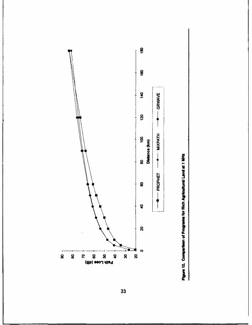
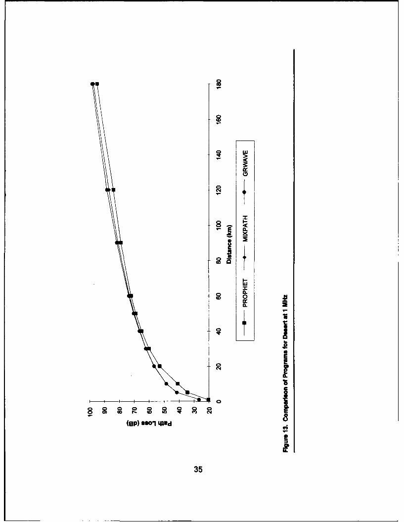
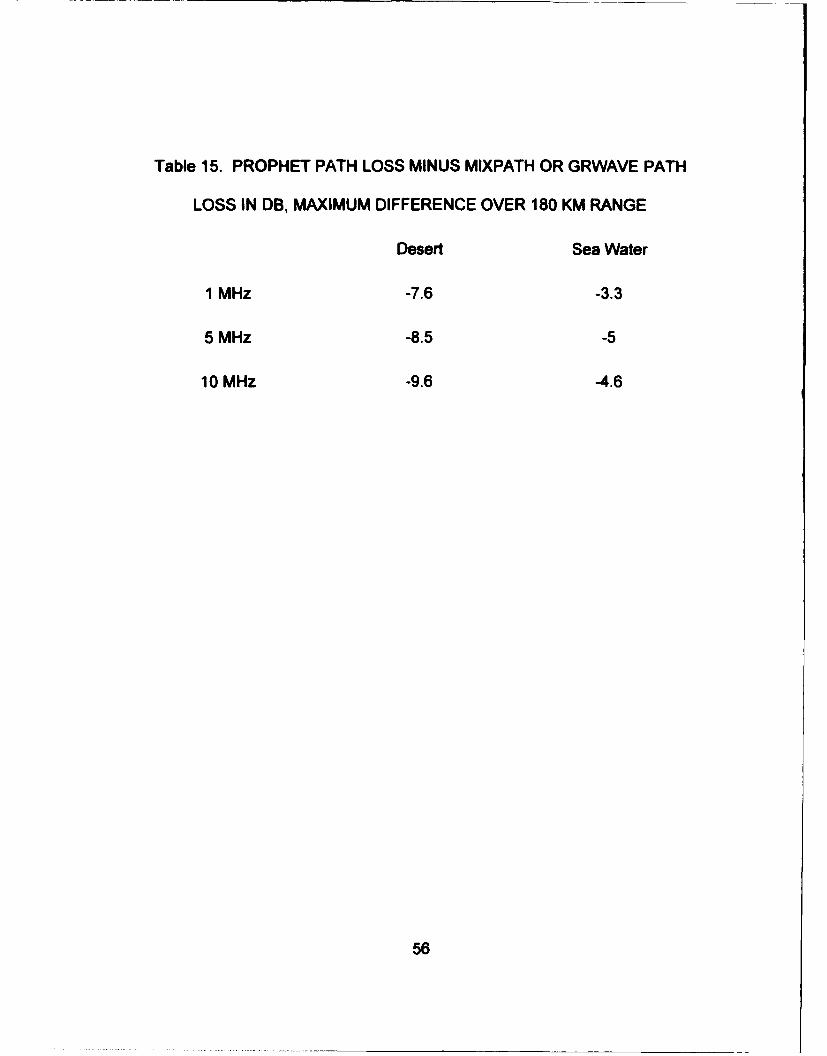
HF groundwave field strength predictions by PROPHET were 3 to 10 dB stronger

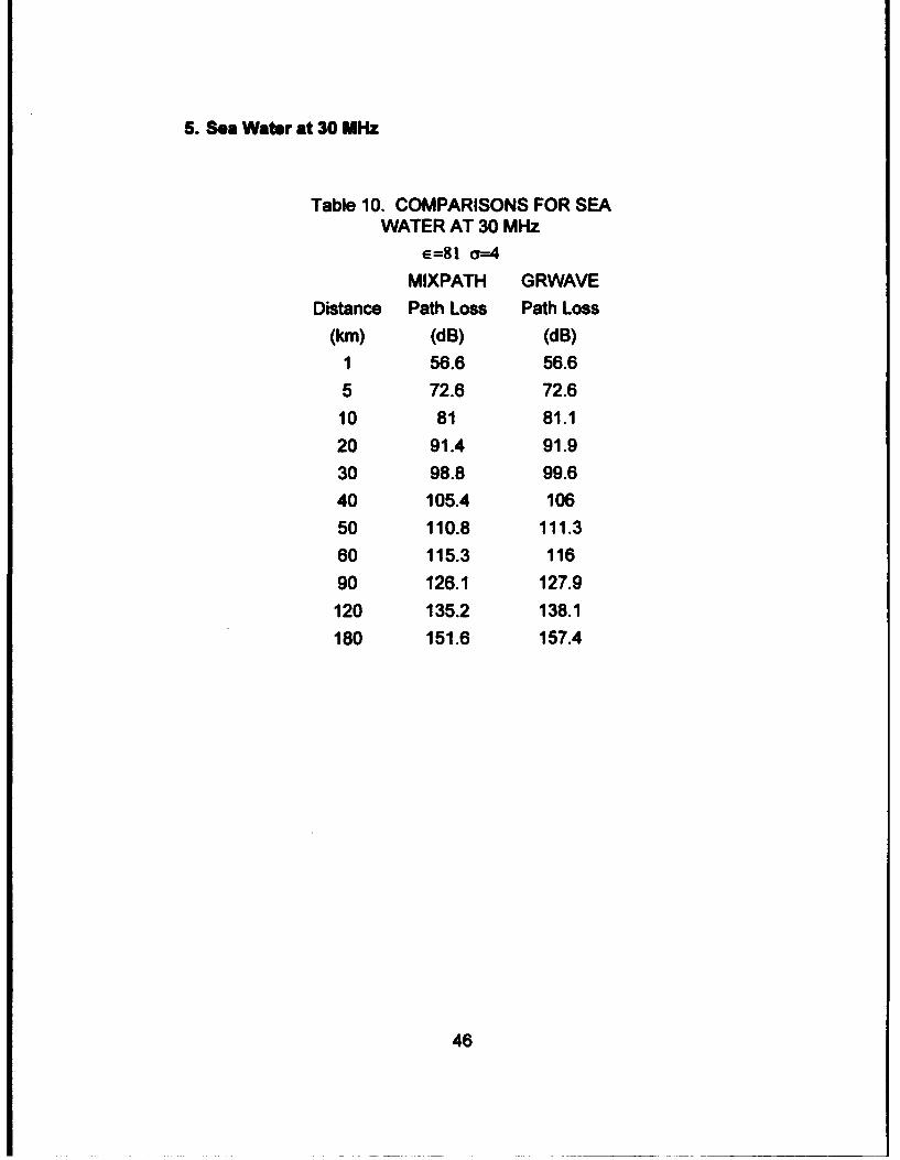
than those of the other programs. GRWAVE and MIXPATH field strength

predictions were in close agreement, the difference generally being less than I or

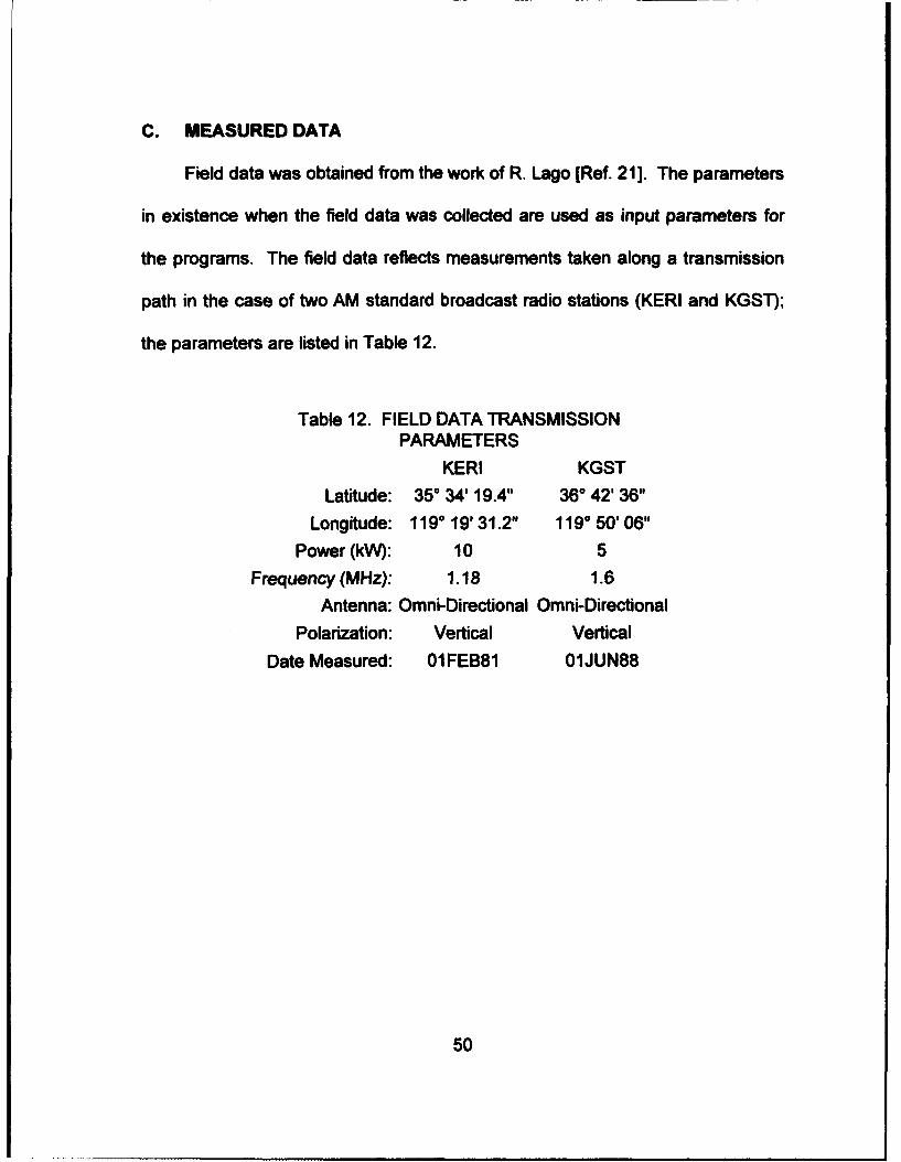
2 dB. Field measurements of path loss for two AM broadcast frequencies were

evaluated by comparison with estimates provided by ADVANCED PROPHET.

The measured groundwave field strengths were found to be from 8 dB weaker at

short distances to 18 dB stronger at large distances. It is recommended that

future efforts be directed toward improving and validating the accuracy of the

groundwave propagation models used in these programs. It is also

recommended that more extensive documentation be developed for GRWAVE.

pr'T 7AT,-J INSPECTED 5

Av ;libii•' •.ydes

Aval1 a,ý iorDist Special

ff1l

CONTENTS

I. INTRO D UCTIO N .......................................................... I

II. THEORETICAL BACKGROUND ......................................... 4

A. GROUNDWAVE PROPAGATION THEORY ............................ 4

1. Groundwave Defined .............................................. 5

2. Simple Variables in Propagation .................................... 6

3. Antennas Located on the Surface ................................... 7

4. Antennas Above the Surface ...................................... 10

B. PARAMETERS INFLUENCING PROPAGATION .................... 11

1. Penetration Depth ................................................ 11

2. Ground Conductivity .............................................. 12

3. Terrain Irregularities ............................................. 12

4. V egetation ....................................................... 12

5. Surface C lutter ................................................... 13

C. GROUNDWAVE APPLICATIONS ................................... 13

II1. DESCRIPTION OF PROGRAMS ...................................... 15

A. THE MIXPATH PROGRAM .......................................... 15

iv

1. A pproach ......................................................... 15

2. The Com puter Model ............................................. 21

3. Input and Output Parameters .................................... 21

B. THE ADVANCED PROPHET PROGRAM ............................ 23

1. A pproach ........................................................ 23

2. The Computer Model ............................................. 23

3. Input and Output Parameters .................................... 24

C. THE GRWAVE PROGRAM .......................................... 26

1. A pproach ........................................................ 26

2. The Computer Model ............................................. 26

3. Input Parameters ................................................ 27

IV. COMPARISON OF PROGRAMS ...................................... 28

A. COMPARISONS FOR VARIOUS GROUND TYPES AT 1 MHZ ....... 28

1. Sea W ater at 1 MHz ............................................. 29

2. Rich Agricultural Land at 1 MHz ................................... 32

3. Flat Desert at I M Hz ............................................. 34

4. Free Space at I M Hz ............................................. 36

V

B. COMPARISONS FOR VARIOUS GROUND TYPES AT 5, 10,

A N D 30 M HZ ....................................................... 37

1. Sea W ater at 5 MHz ............................................. 38

2. Desert at 5 M Hz .................................................. 40

3. Sea Water at 10 MHz ............................................ 42

4. Desert at 10 M Hz ................................................. 44

5. Sea Water at 30 MHz ............................................ 46

6. Desert at 30 M Hz ................................................. 48

C. MEASURED DATA .................................................. 50

7. Station KERI .................................................... 52

8. Station KG ST .................................................... 53

V. CONCLUSIONS AND RECOMMENDATIONS .......................... 54

A PPEN DIX ............................................................... 57

LIST OF REFERENCES ................................................... 58

INITIAL DISTRIBUTION LIST ............................................. 60

vi

LIST OF FIGURES

Figure 1. Range Characteristics of HF Propagation ........ .......... 3

Figure 2. Components of the Groundwave .................................. 5

Figure 3. Surface Wave Zones ........................................... 9

Figure 4. Effect of Ground Type on the Sommerfeld Zone ................... 9

Figure 5. Engineering System Model ..................................... 16

Figure 6. Transmission Path with Three Different Segments ................ 18

Figure 7. Effects of a Mixed Propagation on the Field Strength Curve ....... 20

Figure 8. Output Format for MIXPATH .................................... 22

Figure 9. PROPHET Output Format ....................................... 25

Figure 10. GRWAVE Output Format ....................................... 27

Figure 11. Comparison of Programs for Sea Water at 1 MHz ............... 31

Figure 12. Comparison of Programs for Rich Agricultural Land at I MHz .... 33

Figure 13. Comparison of Programs for Desert at 1 MHz ................... 35

Figure 14. Comparison of Programs for Sea Water at 5 MHz ............... 39

Figure 15. Comparison of Programs for Desert at 5 MHz ................... 41

vii

Figure 16. Comparison of Programs for Sea Water at 10 MHz .............. 43

Figure 17. Comparison of Programs for Desert at 10 MHz .................. 45

Figure 18. Comparison of Programs for Sea Water at 30 MHz .............. 47

Figure 19. Comparison of Programs for Desert at 30 MHz .................. 49

viii

LIST OF TABLES

Table 1. PENETRATION DEPTH FOR DIFFERENT GROUND TYPES ..... 11

Table 2. COMPARISONS FOR SEA WATER AT 1 MHz ................... 30

Table 3. COMPARISONS FOR RICH AGRICULTURAL LAND AT 1 MHz... 32

Table 4. COMPARISONS FOR FLAT DESERT AT 1 MHz ................. 34

Table 5. COMPARISONS FOR FREE SPACE AT 1 MHz .................. 37

Table 6. COMPARISONS FOR SEA WATER AT 5 MHz ................... 38

Table 7. COMPARISONS FOR FLAT DESERT AT 1 MHz ................. 40

Table 8. COMPARISONS FOR SEA WATER AT 10 MHz .................. 42

Table 9. COMPARISONS FOR FLAT DESERT AT 10 MHz ................ 44

Table 10. COMPARISONS FOR SEA WATER AT 30 MHz ................. 46

Table 11. COMPARISONS FOR FLAT DESERT AT 30 MHz ............... 48

Table 12. FIELD DATA TRANSMISSION PARAMETERS .................. 50

Table 13. MEASURED PATH LOSS, STATION KERI (1.18 MHz, 10 kW) ... 52

Table 14. MEASURED PATH LOSS, STATION KGST (1.6 MHz, 5 kW) .... 53

ix

I. INTRODUCTION

This thesis is concerned with high-frequency (HF) communications systems,

which provide an alternative to line-of-sight (LOS) satellite communications both

by means of ionospheric skywave and groundwave propagation. HF military

communications are in the frequency range of 2 to 32 MHz. HF wave

propagation has three components: the sky, space, and ground waves. A

problem inherent to HF communications, and the specific area of concern in this

thesis, is to accurately predict the received signal level, commonly measured by

field strength over given paths. Since the beginning of the twentieth century,

scientists have worked to develop methods of predicting losses in field strength

(path loss) based on known transmission parameters (distance, power, ground

characteristics, etc.).

The groundwave component of the HF wave (HFGW) can provide unique

capability for communications, as illustrated in Figure 1, and is important in a

variet, of military applications. It must be accurately modeled to predict tactical

communications performance including interference from jamming sources, and

to predict communications in difficult geographical environments (such as the

ljord environment or mountainous terrain). Of course, the groundwave is

essential for commercial broadcast beyond LOS. Because path loss increases

I

rapidly with frequency, most groundwave propagation applications are at or below

the low end of the HF band, less than a few MHz. There has been some interest

at higher frequencies, since HFGW communications in the 20 to 30 MHz band

have also been empirically proven to be nuclear-survivable, with non-LOS ranges

as high as 115 km [Ref. 11. In this thesis, to accommodate the entire range of

interest, the groundwave propagation models were compared for the entire range

of 1 MHz to 30 MHz.

Various computer modeling programs have been developed to accurately

predict HF propagation modes. The principal objective of this report is to

compare the field strength predictions of these programs. In Chapter 11 the

theoretical background of groundwave propagation is introduced. In Chapter 111,

the three computer programs to be compared are discussed, along with the

models upon which they are based. Chapter IV presents comparisons based on

various transmission frequencies and ground constants. In addition, measured

AM broadcast path loss is compared with loss predicted by one of the programs.

In Chapter V, conclusions are presented and recommendations made.

2

Intsrmediate Intemlediaterange arng@

IntrOhW'lWC Limit of Silent Skipzone ground vi zone distance

The diagram on the left illustrates the coincidence of groundwave and

skywave components, while the diagram on the right illustrates asituation in which the groundwave is the only effective method oftransmission due to range.

Figure 1. Range Characteristic of HF Propagation [Ref. 21.

3

II. THEORETICAL BACKGROUND

A. GROUNDWAVE PROPAGATION THEORY

Since the advent of HF communications there has been a great deal of

research into the propagation of waves. In 1909, Sommerfeld expressed the

solution for a vertical electrical dipole on the plane interface between an insulator

and a conductor, and divided the expression for the field into a "space wave," and

a "surface wave," proposing a somewhat complex series of expressions to

explain propagation over a flat, smooth earth [Ref. 3]. Van Der Pol and Bremmer,

in 1937, made it possible to calculate field strengths at distant F oints, using

residue series [Ref. 4]. In 1941, Norton made Sommerfeld's theory a more

practical proposition for communications engineers, and introduced expressions

to account for a spherical earth [Ref. 5]. Millington introduced a semi-empirical

method to give fairly accurate results for a path with some variation in the earth's

constants in 1949 [Ref. 6]. Hufford, in 1952, developed an integral equation for

arbitrary changes of both the earth's constants and shape along the path [Ref. 7].

Since that time many individuals and organizations have conducted research into

the various influences upon propagation, but a simplified model to partially explain

the phenomenon is possible.

4

1. Groundwave Defined

"Groundwave" describes the total field (the line of sight, ground surface

reflection, and surface waves) observed at a point in space due to a radiation

source located a finite distance above the earth, as illustrated in Figure 2.

Generally, vertical polarization is required, as horizontal polarization would

generate no appreciable ground wave. Any wave component reflected from the

ionosphere or upper atmospheric layer (e.g., troposcatter) is excluded, but the

groundwave does include effects resulting from knife-edge and earth-spherical

diffraction. The line of sight (or direct) wave and the ground reflected wave are

together known as the space wave.

Direct WaveSpaceWave IGround Reflected Wave

Surface Wave

XMT Antenna RCV Antenna

Figure 2. Components Of The Groundwave.

5

HF frequencies in the range 2-32 MHz are employed in groundwave

communications, but at frequencies above about 4 MHz strong attenuation may

occur [Ref. 21. Above approximately 30 MHz, there is relatively little interest for

communications.

2. Simple Variables in Propagation

The International Radio Consultative Committee (CCIR) has adopted the

following equation to determine the root mean square (rms) field strength:

E0= 300pd, (1)

where E0 is in volts per meter, Pk is the transmitted power in kilowatts, and d is

the range in meters [Ref. 2]. This assumes a very short vertical dipole near a

perfectly conducting ground, and is therefore only the starting point for

determining field strength at a given distance from the transmitter.

Three ground characteristics affecting groundwave propagation must also

be considered in order to account for the lack of perfectly conducting ground:

"* Relative Permeability - normally regarded as unity and therefore seldom a

factor in propagation problems;

"• Relative Dielectric Constant- e;

"* Conductivity - a (expressed in siemens per meter).

Note that older literature uses the unit "mhos per meter" which is identical to

siemens per meter.

6

The influence of the latter two factors upon wave propagation is

expressed by

E / =E -60iacX. (2)

This is a complex dielectric constant relative to free space, where X is the free

space wavelength in meters [Ref. 2]. The effects of ground electrical

characteristics are then illustrated by

E/Eo= 1 + Rei +(1 - R)Ae + .. (3)DirectWave RefectedWave SurfaceWave Induction Field And Secondary Effects

where R, A, and A are all functions of e', R is the complex reflection coefficient of

the ground for the wave polarization of interest, A is the surface wave attenuation

factor, and A is the phase difference caused by the path difference between the

direct and ground reflected waves [Ref. 8].

3. Antennas Located on the Surface

If the transmitting and receiving antennas are both located on the surface

uf the earth, the radiated field can be expressed as

E = KFP1/2/d, (4)

where P is the total radiated power, K is a constant which depends upon the

antenna characteristics, and F is a factor which depends on frequency, ground

7

characteristics, polarization, and distance; it decreases with increasing frequency

and/or decreasing ground conductivity, and is much smaller for horizontal than

vertical wave polarization. An increase in the value of F denotes a decrease in

path loss, and vice versa.

When antennas are located on the surface, the direct wave and the

ground reflected wave will cancel each other out, leaving only the surface wave,

which travels along the surface through three successive zones (illustrated in

Figure 3):

"* The Direct Radiation Zone, where the radio waves travel a short distance as

though through free space, and the attenuation factor is equal to unity;

"* The Sommerfeld Zone, where the radio waves travel in a manner described

by the Sommerfeld Flat Earth Theory [Ref. 3] and the factor F becomes

proportional to 1/d. As shown in Figure 4, the boundary between the Direct

Radiation Zone and the Sommerfeld Zone depends upon the nature of the

ground.

"• The Diffraction Zone, where the Earth's curvature begins to play a role and

the factor F Lacomes independent of ground conductivity (approximately

0.62IX. dB/km).

8

ONE SOMMERFELD ZONE DIFFRACTION ZONE

dhkamd

FIgure 3. Surface Waoe Zonge [Ref. 2].

- 00SOMMERFELD ZONE DIFFRACTIONZONE-

10.gmd typ)e.

Figure 4. Effect Of Ground Type Oni The Sommeufel Zone [Ref. 21.

9

4. Antennas above the surface

As the heights of the antennas are increased above ground level, it is

necessary to modify Equation 4 to express

dKFPI/2 H(h1 )H(h 2) (5)

where H(h) is the height gain factor for an antenna at height h above the surface

and h, and h2 are the heights of the transmitting and receiving antennas,

respectively.

When antenna height above ground exceeds 35X2.3, the Earth's surface

plays a smaller role, and the space wave (line-of-sight and reflected waves)

predominates. The space wave encounters three zones of propagation as it

travels:

"* The Interference Zone, where the direct wave and the ground reflected

wave are summed to derive the total field;

", The Radio Horizon Zone, where the surface wave may contribute to the

total field; and,

"* The Diffraction Zone, where, as for the surface wave, attenuation loss has

settled to a constant value.

10

B. PARAMETERS INFLUENCING PROPAGATION

While the above discussion presents methods of determining propagation,

there are complications arising from the determination of the variables used and

from other influential factors.

1. Penetration Depth

The penetration depth 8 is defined as the depth at which the wave has

been attenuated to 1/e (37%) of its value at the surface. Also known as "skin

depth", this factor depends on the values of the effective Earth constants as

shown in Table 1.

Table 1. PENETRATION DEPTH FOR DIFFERENT GROUND TYPES 10

MHz FREQUENCY [Ref. 2]

GROUND TYPE PENETRATION DEPTH (m)

Sea Water 0.1

Wet Ground 3

Fresh Water 10

Medium Dry Ground 15

11

2. Ground Conductivity

Factors influencing conductivity include moisture content and

temperature. In addition, it is necessary to consider the general geologic

structure of the path, as well as loss due to absorption by surface objects.

3. Terrain Irregularities

Shadowing which may occur in certain locations as a result of terrain and

terrain irregularities may result in attenuation and phase differences for received

signals. The effect on the field strength produced by terrain irregularities varies

with the frequency of transmission and the specific characteristics of the

irregularity. Mountainous terrain may actually increase signal strength through

knife-edge diffraction, a phenomenon known as obstacle gain. Although part of

the groundwave, diffraction is not covered in this thesis, but it is modeled in such

programs as the Terrain-Integrated Rough-Earth Model (TIREM), which was

developed to calculate the basic propagation loss over irregular terrain at

frequencies between 1 MHz and 20 GHz.

4. Vegetation

Vegetation along the propagation path also influences field strength. For

instance, a densely forested area will produce different propagation results than

one with no vegetation, and the effect will depend on whether the forest is in leaf,

wet, or covered in snow. Below about 2 MHz, a forest environment has little

effect on the groundwave.

12

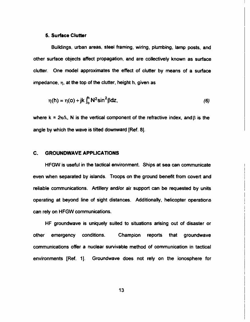
5. Surface Clutter

Buildings, urban areas, steel framing, wiring, plumbing, lamp posts, and

other surface objects affect propagation, and are collectively known as surface

clutter. One model approximates the effect of clutter by means of a surface

impedance, T1, at the top of the clutter, height h, given as

71(h) = rj(o) +jk ro N2sin 2I3dz, (6)

where k = 21cA, N is the vertical component of the refractive index, and f3 is the

angle by which the wave is tilted downward [Ref. 8].

C. GROUNDWAVE APPLICATIONS

HFGW is useful in the tactical environment. Ships at sea can communicate

even when separated by islands. Troops on the ground benefit from covert and

reliable communications. Artillery and/or air support can be requested by units

operating at beyond line of sight distances. Additionally, helicopter operations

can rely on HFGW communications.

HF groundwave is uniquely suited to situations arising out of disaster or

other emergency conditions. Champion reports that groundwave

communications offer a nuclear survivable method of communication in tactical

environments [Ref. 1]. Groundwave does not rely on the ionosphere for

13

propagation of the signal, and therefore is not susceptible to ionospheric

conditions resulting from EMP.

HFGW is also useful for nighttime short-range weather net data at rates of

up to 2400 baud. In the range of 20 to 30 MHz, communication by HFGW has

been proven effective in fjords. In areas where terrain prohibits the laying of

telephone wire, HFGW can provide an ideal and low-cost communication link.

14

Ill. DESCRIPTION OF PROGRAMS

A. THE MIXPATH PROGRAM

1. Approach

The Department of Defense (DOD) Electromagnetic Compatibility

Analysis Center Technology Transfer Program (ECAC-TTP) software package

MIXPATH predicts groundwave propagation over a smooth earth having more

than one propagation medium. This program employs Millington's meihod of

computing surface wave transmission loss, which is highly dependent on the

conductivity and dielectric constants of the Earth. MIXPATH is used in

combination with the ECAC Far-Field Smooth Earth Coupling Code (EFFSECC)

model, which differentiates between path distances short enough to assume

planar earth and longer distances, at which the earth's curvature begins to play a

significant role.

In 1949, G. Millington introduced a semi-empirical method to give fairly

accurate results for quantifying the effect of propagation over mixed terrain [Ref.

6]. This procedure is known as Millington's Model, and assumes a semi-infinite

half-space earth with a smooth surface, considering homogeneous conductivity

and permittivity throughout the path. Each homogenous segment along the

multiple-segment path has its own conductivity and dielectric constants, which are

15

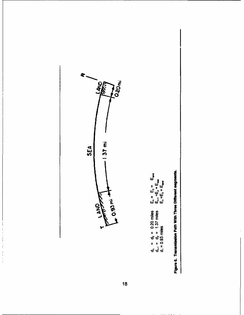
combined via computational averaging. The irregularities presented by the terrain

are disregarded, and the antenna height-gain function is applied to the transmitter

and receiver to compensate for their respective heights. Figure 5 illustrates the

procedure used to compute the groundwave field strength for zero-height

antennas over a path with distinct boundaries.

dT = Total path of distance

d, = Length of segment #1

d2 = Length of segment #2

d3 = Length of segment #3

d,= Length of segment #4

d. = Length of segment #n

a, E = Permittivity and conductivity of segment #1

a 2e2 = Permittivity and conductivity of segment #2

C3 e E= Permittivity and conductivity of segment #3

aE,= Permittivity and conductivity of segment #4

avr ,= Permittivity and conductivity of segment #n

Figure 5. Engineering System Model

Transmission field strength is derived from

kTR - l(dj)F 2(dl+d2 ) (7)-- 2(d )(

16

for the transmitter, where 41 (dj) is the field strength at a distance d, over an earth

having constants al and El, 42 (dj+d 2) is the field strength at a distance cd+d 2 over

an earth having constants a 2 and E 2 , and 42(d,) is the field strength at a distance

d, over an earth having constants a 2 and E2; and

4RT = 2(d2Yj (d2+dl)(8=RT - • 1 (d 2 ) (8)

for the receiver. The two equations yield the geometric mean of the values by

4d = 1TR4RT (9)

For n boundaries, the field strength in dB expressed at dn is given by the following

equations:

ETR(dB) = Ej(d1)+ E2(di +d 2)+ E3(d1 +d 2 +d 3)... + En(dT) (10)-E2(d1) - E3(d 1 + d2) ... En(d, + d2 +... + dn-1)

ERT(dB) = En(dn) + En- (d + d.n-) +... + E l(dT) (11)-E n-i(d n)-.. E 1(dn + dn-i +.. +d 2)

Ed = ETR+ERT (12)2

Figure 6 illustrates a transmission path which is composed of an initial

0.93 miles of land, a 1.37 mile segment of sea water, and a final 0.20 mile

segment of land.

17

U)J

ON! In111± E

liw

- ~11W'04 I

18uh

The effects of this mixed path upon the field strength are illustrated in

Figure 7. Three ground segments are modeled; the first is the circular region

centered on the transmitter with radius of 0.93 sm (statute mile). The second is

the ring between 0.93 and 2.3 sm radius, and the third is the region beyond 2.3

sm radius. The field strength curve for the first segment matches that of a land

path, but experiences a sharp deviation from the land path curve when it

encounters the second segment, which is composed of sea water. Note that the

field strength curve does not correspond to the sea water path curve while in the

sea water segment, but merely moves toward the sea water path curve. This

phenomenon is known as "recovery effect," and illustrates the effect of the sea

water segment on the field strength curve that has already passed through a land

segment. The field strength curve moves back into correspondence with the land

path curve as the path encounters the final land segment of the transmission

path, but previous passage through a sea water path prohibits the field strength

curve from actually rejoining the land path curve as it completes the passage

through the transmission path.

19

lOO

- U00 v

3S\

Ic -

Y 4.

GRUN GROU 0%1

402

GAONO AGFE OAND

DIS'TANICE (STATITUI'T MiLE[S)

Figure 7. Effects Of A Mixed Propagation Path On The Field Strength Curve.

20

2. The Computer Model

The ECAC model differentiates between distances that are short enough

to assume a planar earth and those long enough that the earth's curvature begins

to play a role. The separation distance, dc, between the planar and curved earth

models was found empirically.

When antenna separations exceed dc, the earth's curvature begins to

play a role. The ECAC model fits this added loss as increasing linearly with

distance, and the major part of this calculation is to determine the slope of this

increase.

3. Input and Output Parameters

MIXPATH predicts propagation based on the input parameters for

antenna and feed height and polarization, distance, number of differing path

segments, and permittivity, conductivity, refractivity, and surface type for each

path segment. An example of output from the MIXPATH Program is shown in

Figure 8.

21

a.4 OI..cmammeamOIm cae Qm

. . . . . . . . . .. ... ..

. • .CUO ...................

Al 3• i o• ,l

V T- .• .; . .... ....~M .. . ! Ism--

u 0 • 0•_

-,as

a A

I • • I~ • Ii I ~ i llOi

i - 29 04

Idm o -- oI • •• i le i l e ~ l

*.d ewe ei , *II *0. eIeO I I e 0 e OO •

F.M. * ::HHHHHHHHU~e

" "M. f *-s: ...60.. .... . ..

* m, ~ dos4 *a

NOWO

.2 i." . :. .. d; -- d'd ::::::: ::

tooo i •

". . a. .* m S..

0 afle .60**0 08.@ 40 40- 0M M 0w x

•0"oo Mooo.4:-- ~ ~~~~W-Z wv.seeeoeseee,,,,....... ..,, ..... .....

II :1 ... ii i ! ,,,,::

we

402 00

S" .*" a.' °..e0-0-- .s.-/22

,,_,, ,mc. .... , ,.ee...*i.iili i6i.a...,,,

mat .e....*****.*.iii" .*_mil lulw.. • -.• • oil

36 l "..-.-........-...--0 in

Io i lO .I...°.. .. o.• •.... -C==

. -------------------- m=C.. o . i4 ~ ~ oJ-ialelllo

* .. i I~:dldein*S2::IdIdZla:dd I

22

B. THE ADVANCED PROPHET PROGRAM

1. Approach

ADVANCED PROPHET (AP) is a collection of computer simulation

models developed to support tactical use of the HF band (2-32 MHz). For

simplicity, the program title "PROPHET" designates ADVANCED PROPHET

throughout this report. PROPHET can be used to determine:

* Existence of an HF skywave channel between two sites anywhere in

the world,

# The potential for a hostile force to intercept the transmission, to

radiolocate the transmitter, or to jam the reception site,

* Groundwave for short range circuits (for instance, it can analyze

communications between closely operating units).

To predict groundwave propagation, the program calculates the surface

loss from the designated transmitter to the designated receiver. There are three

output options; one lists the data in tabular form and the other two produce plots

of maximum range versus frequency for the given transmitter power or maximum

range versus power for the specified frequency.

2. The Computer Model

PROPHET can access four different models for determining groundwave

propagation: ECAC, Booker-Lugannani, Levine, and EPM-73 [Ref. 9]. ECAC

was discussed in the previous section.

23

Booker and Lugananni model the work of Barrick [Ref. 10, 11, 12],

deriving an empirical model that considers the surface wave losses for antennas

at sea surface, using signals which are vertically polarized [Ref. 13].

The Levine model is employed for low-antenna height,

smooth-ocean-surface propagation [Ref. 14]. Loss is written in two terms, with a

free space loss related term, and an approximation accounting for the additional

losses due to curvature and finite earth conductivity:

EPM-73 (the Lustgarten/Madison empirical propagation model) includes

calculations for direct ray, reflected ray, and the surface wave, and also considers

troposcatter effects at greater distances [Ref. 15].

The model has two sections, determined by the ratio of the antenna

height (h) to the wavelength (k). The high-h/k section has three regions of

interest: the reflection region, the diffraction region, and the troposcatter region.

3. Input and Output Parameters

PROPHET accepts as input parameters the frequency and range of

transmission, transmitter power, transmitter gain, antenna heights and

polarization, required bandwidth, signal to noise ratio, terrain type, wind velocity,

surface conductivity and dielectric constant, and man-made and atmospheric

noise models. The program outputs the calculated groundwave transmission

path loss and the required power for transmission. Output format for PROPHET

is shown in Figure 9. Although not explained in the PROPHET user's manual, in

24

order to perform goundwave calculations based on user-defined constants, it is

necessary to enter the terrain type as US.

*** UNCLASSIFIED *** DATE: 2/ 1 AT 12:48 UTGROUNDWAVE FROM KGST ON: 1.600 MHZ

RANGE TO RCVR TEMP RANGE IS: 17.6 KMTRANSMIT GROUNDWAVE GAIN: .o dBi

POLARIZATION: VTRANSMIT ANTENNA HEIGHT: .0 METERS

RECEIVE ANTENNA HEIGHT: .0 METERSTRANSMITTER POWER: 5000.0 WATTS

REQUIRED BANDWIDTH: 2.8 KHZREQUIRED SIGNAL TO NOISE: 12.0 dB

TERRAIN: usSURFACE COVER: CL

SURFACE CONDUCTIVITY: .1OE-02 MHO/MDIELECTRIC: 15.00

MANMADE NOISE MODEL: QRATMOSPHERIC NOISE: NO

CALCULATED GROUNDWAVE LOSS: 79.00 dBREQUIRED POWER: .084 WATTS

AVAILABLE POWER: 5000.000 WATTSMAX RANGE FOR POWER OF 5000.000 WATTS: 192.4 K4

NOTE: RECEIVE ANTENNA GROUNDWAVE GAIN ASSUMED - 0.0 dBiRange to RCVR Temp Range is a parameter which allows the user to

override computed distance (based on latitude and longitude). The

terrain parameter "US" denotes values calculated from the user input

values for permittivity and conductivity. The surface cover parameter

value "CL" indicates a clear surface, and the noise model parameter

"QR" indicates levels of manmade noise found in a quiet rural

environment.

Figure 9. PROPHET Output Format

25

C. THE GRWAVE PROGRAM

1. Approach

GRWAVE was developed by Leslie Berry at the Institute for

Telecommunications Sciences in Boulder, Colorado. The program was modified

for execution on a PC by Dr. John Cavanagh of the Naval Surface Warfare

Center in July of 1988. Later, CCIR adopted the program to compute

groundwave transmission loss. The program can be used to determine

transmission loss and field strength transmission loss from the designated

transmitter to the designated receiver.

2. The Computer Model

The GRWAVE model considers a smooth, homogeneous earth bounded

by a troposphere with exponential height variation. GRWAVE uses three different

methods to calculate field strength. At longer distances, the residue series is

used, at shorter distances, the model employs the extended form of the

Sommerfeld flat-earth theory, and geometric optics are used to calculate field

strengths at distances not covered by either residue series or the Sommerfeld

theory [Ref. 16]. An examination of the code shows that the program uses five

subroutines: geometric optics (GWGO); a flat earth attenuation function using

King's Equation (Eq. # 21, 1969) with curvature correction from Hill and Wait

(GWFEC); Hill and Wait's (1980) series for small Q (GWSQ); a residue series

module (GWRSS); and numerical integration (GWINT).

26

Unfortunately, the documentation for this program was never completed,

therefore all of the information presented here was derived from a limited

interpretation of the actual program code. A more thorough understanding of the

program's operation is dependent upon further analysis.

3. Input Parameters

GRWAVE requires frequency, polarization, power, ground dielectric

constant, lower and higher antenna heights, and distance. The output is

illustrated in Figure 10.

GW84 CALCULATIONFREQUENCY - 1.180 3KZ, VERTICAL POLARIZATION. ERP - 10. 00 KW

GROUND CONSTANTS: (4.0000,81.0). (EFFECTIVE RADIUS)/(TRUE RADIUS) - 1.000LOWER ANTENNA AT • 0 X, 1ItER ANTENNA AT .0 X

DISXK E, D3U TX LOSS, DB PS TX LOSS20.76 93.0 54.4 60.2324.70 91.5 55.9 61.74

E, DBU is the field strength expressed in dB.

TX LOSS, DB is the transmission loss expressed in dB.

FS TX LOSS is the free space transmission loss expressed in dB.

Figure 10. GRWAVE Output Format.

27

IV. COMPARISON OF PROGRAMS

In this chapter, three of the programs described in Chapter III (PROPHET,

MIXPATH, and GRWAVE) are compared with respect to the predicteo field

strength loss. In Sections A and B, the losses are compared for various ground

types for distances from 1 to 180 km. Section C contains a comparison of

measured field strengths and predictions by PROPHET. Although most

groundwave applications occur at frequencies below 4 or 5 MHz, the

comparisons were extended to 30 MHz, since there is one proposed application

relating to nuclear survivable communications at this frequency [Ref. 1,

A. COMPARISONS FOR VARIOUS GROUND TYPES AT 1 MHz

In this section, path loss predictions at 1 MHz are compared as a function of

ground type and distance over a range of I to 180 km. Values for permittivity and

conductivity were chosen to reflect the characteristics of sea water, rich

agricultural land, flat desert, and free space. These values, and those for other

types of transmission paths, are listed in Appendix A. Other parameters

common to each program are:

"* Power: 10kW

"* Antenna: Omni-directional.

28

"* Antenna Height: 0 m.

"* Modulation: SSB.

"* Bandwidth: 2.8 kHz.

"* Polarization: Vertical.

"* Surface Cover: Clear.

"• Effective Radius/True Radius = 1.

1. Sea Water at I MHz

Table 2 and Figure 11 present a comparison of path loss predictions

obtained for ground constants representing sea water. As indicated, MIXPATH

and GRWAVE agree within 1 dB over the entire range of distances from 1 to 180

km. PROPHET provides 2 to 3 dB lower estimates of path loss throughout the

transmission range.

29

Table 2. COMPARISONS FOR SEA WATER AT 1 MHz

e=81 a=4PROPHET MIXPATH GRWAVE

Distance Path Loss Path Loss Path Loss

(km) (dB) (dB) (dB)

1 23.94 26.4 26.4

5 37.92 40.4 40.4

10 43.94 46.4 46.4

20 49.96 52.5 52.6

30 53.48 56 56.2

40 55.98 58.5 58.8

50 57.92 60.4 60.9

60 59.5 62 62.6

90 63.03 65.6 66.6

120 65.52 68.1 69.8

180 70.6 73.9 74.8

30

m0:

CL

, ~i ±

EE

I-G F-m 0

(OP) 901 W~td

31

2. Rich Agricultural Land at I MHz

Predicted path loss is listed in Table 3 and displayed in Figure 12.

GRWAVE and MIXPATH agree within 2 dB over all distances. PROPHET's path

loss estimates in this environment are as much as 7 dB smaller than those of

MIXPATH and GRWAVE, which is a significant difference.

Table 3. COMPARISONS FOR RICHAGRICULTURAL LAND

AT 1 MHz

6=20 =--0.04

PROPHET MIXPATH GRWAVE

Distance Path Loss Path Loss Path Loss

(km) (dB) (dB) (dB)

1 20.42 26.5 26.5

5 34.4 40.7 40.7

10 40.42 47.1 47.1

20 46.44 53.6 53.8

30 49.96 57.7 57.940 53.76 60.8 61.1

50 57.63 63.3 63.6

60 60.8 65.4 65.9

90 67.84 70.5 71.3120 72.84 74.5 75.8

180 83.37 81.3 83.2

32

co

CL0

a.

lac

C*4ILV

(SP) SMI Wd C4

33

3. Flat Desert at I MHz

Path loss predictions for a flat desert environment are listed in Table 4

and displayed in Figure 13. MIXPATH and GRWAVE path loss values agree

within 2 dB for all distances. PROPHET's loss estimates are up to 7.6 dB smaller

than those of MIXPATH and GRWAVE.

Table 4. COMPARISONS FOR FLAT DESERT

AT 1 MHz

r-=4 a=O.O1

PROPHET MIXPATH GRWAVE

Distance Path Loss Path Loss Path Loss

(km) (dB) (dB) (dB)

1 20.42 26.7 26.7

5 34.4 41.5 41.5

10 40.89 48.5 48.5

20 52.93 56.5 56.6

30 59.97 61.9 62

40 64.97 66.2 66.4

50 68.85 69.9 70.2

60 72.01 73.1 73.5

90 79.06 81 81.8

120 84.06 87 88.3

180 95.15 97.7 98.5

34

0

CM

8o

N

I "a-

IS

(OP) lOwl 448zd

35

4. Free Space at I MHz

As a validity test of the programs, the predictions for the simplest of

environments, free space, were compared with the exact solutions provided by

the laws of physics. Only the LOS path exists with no interfering matter between

transmitter and receiver. In the far field, the field strength varies inversely with

distance, d, so the loss, in dB, should vary as 20logd. The far field extends from

2D2/%. to infinity where D is the antenna dimension and X the wavelength. For I

MHz, the wavelength is 300m, so the far field condition is satisfied beyond

d=150m in the case of a typical vertical (omnidirectional) dipole antenna. For free

space, e=1 and a=0. Since the programs do not accept a=0, a=1x10a mho/m

was used. MIXPATH would not accept values below 0.001 mho/m so it was

omitted from the comparison. It can be seen that the complex dielectric constant

becomes &'=1-0.018i which is reasonably close to the free space value ofe'=1.0.

Table 6 lists the program predicted path loss when permittivity and conductivity

are adjusted to reflect a free space environment. For each program, predicted

path loss is compared to the exact loss calculation, where the latter was adjusted

to agree at d=1 km. The large departure of the program predictions from the

theoretically exact losses could not be explained since the source codes and/or

documentation were not available. Another test is to consider a half-space of

infinite conductivity. This is approximated by sea water. In this case, the 20logd

behavior of the predicted losses is clearly present in the tabulated results (see

36

Table 2). The 201ogd behavior is expected for all three programs since the far

field of an antenna above an infinitely conducting half-space is equivalent to the

superposition of the fields of the antenna and its image source, both located in

free space.

Table 5. COMPARISONS FOR FREE SPACEAT 1 MHz

Distance Relative Path Loss in dB

(km) PROPHET 20logd GRWAVE 20logd

1 20.42 20.42 32.5 32.5

5 39.89 34.4 52.4 46.5

10 51.93 40.4 62.2 52.5

20 63.97 46.4 72.7 58.5

30 71.01 50 79.2 62.1

40 76.01 52.5 84 64.6

50 79.89 54.4 87.9 66.5

60 83.05 56 91.1 68.1

90 90.1 59.5 98.7 71.6

120 95.09 62 104.6 74.1

180 106.37 65.5 114.2 77.6

B. COMPARISONS FOR VARIOUS GROUND TYPES AT 5, 10, AND 30 MHz

In Tables 6 and 7, path loss predictions of the programs were compared for

transmission paths over sea water and desert at a frequency of 5 MHz. In Tables

8 and 9, the comparisons were based on a frequency of 10 MHz. The programs

were also compared for transmission paths over sea water (Table 10) and desert

37

(Table 11) for a 30 MHz frequency. At 30 MHz, PROPHET appears to have a

coding error since the path loss predictions were identical for sea water and

desert.

1. Sea Water at 5 MHz

Table 6. COMPARISONS FOR SEA WATER

AT 5 MHz

e=81 a=4

PROPHET MIXPATH GRWAVE

Distance Path Loss Path Loss Path Loss

(km) (dB) (dB) (dB)

1 37.92 40.4 40.4

5 51.9 54.5 54.5

10 57.92 60.6 60.6

20 63.94 66.7 67

30 67.46 70.4 70.8

40 69.96 73 73.7

50 71.9 75.1 76.1

60 73.48 76.8 78.1

90 77.81 82.4 83

120 82.12 86.1 87.1

180 89.25 92.4 94.1

38

IILrr½39U

0.t

) I , €0S• • ( ),,

39I

2. Desert at 5 MHz

Table 7. COMPARISONS FOR DESERTAT 5 MHz

•=4 a=-0.011

PROPHET MIXPATH GRWAVE

Distance Path Loss Path Loss Path Loss

(km) (dB) (dB) (dB)

1 42.77 46 46

5 70.72 74.1 74

10 82.77 87.6 87.6

20 94.81 100.3 100.7

30 101.85 107.5 108.3

40 106.85 112.6 113.950 110.72 116.6 118.5

60 113.89 119.8 122.2

90 125.2 130.2 131.5

120 131.97 137.2 139.2

180 144.03 148.9 152.5

40

Go

IL

0~

Co a

('4

CL

041

3. Sea Water at 10 MHz

Table 8. COMPARISONS FOR SEA WATER AT10 MHz

e =81 a=4PROPHET MIXPATH GRWAVE

Distance Path Loss Path Loss Path Loss

(km) (dB) (dB) (dB)

1 43.94 45.5 46.5

5 57.92 60.7 60.7

10 63.94 67 67.1

20 69.96 73.6 73.9

30 73.63 77.6 78.2

40 77.18 80.7 81.6

50 80.16 83.9 84.4

60 82.79 86.5 86.8

90 89.45 92.8 93.1

120 95.09 98 98.5

180 104.89 107.1 108.2

42

Ui

r'I *a.

qF000 OM 1O

A(OP) $01 lEWd

43

4. Desert at 10 MHz

Table 9. COMPARISONS FOR DESERT AT10 MHz

E --4 o=O.011

PROPHET MIXPATH GRWAVE

Distance Path Loss Path Loss Path Loss

(km) (dB) (dB) (dB)

1 60.64 63.7 63.7

5 88.6 94.1 94.1

10 100.64 106.4 106.6

20 112.68 118.6 119.3

30 119.73 125.7 127

40 124.72 130.7 132.8

50 132.12 136.6 137.4

60 135.55 140.4 141.5

90 144.6 149.9 151.8

120 152.63 157.8 160.7

180 167.22 171.5 176.8

44

0N

III-5

R~~~~ 8 0 0

(SP) 9 l ta,c Lo

45j

5. Sea Water at 30 MHz

Table 10. COMPARISONS FOR SEAWATER AT 30 MHz

c=81 u=4

MIXPATH GRWAVE

Distance Path Loss Path Loss

(km) (dB) (dB)

1 56.6 56.6

5 72.6 72.6

10 81 81.1

20 91.4 91.930 98.8 99.6

40 105.4 106

50 110.8 111.3

60 115.3 116

90 126.1 127.9

120 135.2 138.1

180 151.6 157.4

46

R 8 8 8

(OP) wl W

47C

6. Desert at 30 MHz

Table 11. COMPARISONS FORDESERT AT 30 MHz

e=4 a=0.01 I

MIXPATH GRWAVE

Distance Path Loss Path Loss

(km) (dB) (dB)

1 93.4 93.45 121.6 121.6

10 133.7 134.1

20 145.7 147

30 154.4 155.1

40 160.4 161.450 165.4 166.8

60 169.8 171.6

90 181 184.4

120 191 196

180 209.5 218.4

48

I

co

494

C. MEASURED DATA

Field data was obtained from the work of R. Lago [Ref. 21]. The parameters

in existence when the field data was collected are used as input parameters for

the programs. The field data reflects measurements taken along a transmission

path in the case of two AM standard broadcast radio stations (KERI and KGST);

the parameters are listed in Table 12.

Table 12. FIELD DATA TRANSMISSION

PARAMETERS

KERI KGST

Latitude: 350 34'19.4" 360 42' 36"

Longitude: 119* 19' 31.2" 1190 50' 06"

Power (kW): 10 5

Frequency (MHz): 1.18 1.6

Antenna: Omni-Directional Omni-Directional

Polarization: Vertical Vertical

Date Measured: 01FEB81 01JUN88

50

In the previous section, the PROPHET groundwave field strength (or path

loss) predictions were compared with those of MIXPATH and GRWAVE. In this

section PROPHET predictions are compared with measured data for two AM

broadcast transmitters at 1.18 and 1.6 MHz. The large discrepancies (up to 18

dB) between the predicted and measured data illustrate the difficulty in using the

latter as a yardstick for determining the fidelity of the groundwave models. In

addition to unknown modeling error, the discrepancy can largely be attributed to

the lack of detailed knowledge of the field environment, including ground constant

variation with position and weather, as well as factors such as nearby powerlines

and manmade structures.

51

7. Station KERI

Table 13. COMPARISON OF MEASURED PATHLOSS WITH PROPHET PREDICTIONS, STATION

KERI AT 1.18 MHzField Data PROPHET

Distance Path Loss Path Loss Difference(km) (dB) (dB) (dB)

0.48 N/A N/A N/A

0.97 6.8 N/A N/A

1.45 10.9 6.45 4.45

1.93 13.4 11.42 1.98

2.41 15.6 15.28 0.32

3.06 17.6 19.43 -1.83

3.54 19.4 21.96 -2.56

4.3 20.5 25.34 -4.84

5.07 22.9 28.2 -5.3

6.28 25.3 31.92 -6.62

7.24 26 34.39 -8.39

8.05 26.8 36.23 -9.43

9.5 27.4 39.11 -11.71

11.15 29.5 41.89 -12.39

15.93 33 48.09 -15.09

20.76 37.9 52.69 -14.79

24.7 37.6 55.71 -18.11

52

8. Station KGST

Table 14. COMPARISON OF MEASURED PATHLOSS WITH PROPHET PREDICTIONS STATION

KGST AT 1.6 MHzField Data PROPHET

Distance Path Loss Path Loss Difference(km) (dB) (dB) (dB)

0.4 N/A N/A N/A0.64 4.3 N/A N/A

1.61 12.5 N/A N/A

3.22 19.4 12.04 7.364.8 27.4 18.97 8.43

6.44 28.7 24.08 4.62

8.04 32.2 27.94 4.269.82 34.1 31.41 2.69

12.56 38.3 35.68 2.6216.17 40.6 40.07 0.53

21.57 45.3 45.08 0.22

29.13 48.2 50.3 -2.1

53

V. CONCLUSIONS AND RECOMMENDATIONS

As demonstrated in Chapter 4 GRWAVE and MIXPATH show excellent

agreement up to 60 kilometers, less than 1 dB difference at 1 MHz. GRWAVE

predicts slightly higher path loss than MIXPATH at ranges beyond 60 kilometers,

the maximum difference being 3 dB at ranges from 70 to 180 km. At 1 MHz, the

ADVANCED PROPHET loss averages about 5 dB below those of the other

programs, with the largest difference being 12 dB for free space (zero

conductivity and unity dielectric constant).

At 30 MHz, the maximum difference between the MIXP/IrH and GRWAVE

predictions increases to 9 dB. At 30 MHz and higher frequency, PROPHET

appears to have a coding error, since the predicted loss was indentical for sea

water and desert.

The comparisons of program results with measured field data show that

PROPHET's predictions differ measured path loss by up to 18.1 dB. Large

deviations of predictions from measured path loss unusual and can, in part, be

attributed to lack of knowledge of the field environments, including ground

constants, which can approach 20 dB. Tabiu 15 is a summary of the maximum

differences between PROPHET and MIXPATH/GRWAVE path loss predic,'is

which indicate significant errors.

54

In the limit of an infinite conductivity half-space (approximated by sea

water), the field strength predictions of the three programs exhibit the expected

theoretical d1 distance behavior. In the limit of free space with zero conductivity

(approximated by a = 0.000001 mho/m), the predicted field strength exhibits a

d-'5 to d2 behavior rather than the theoretical d1 law. Since real earth

conductivity rarely is less than 0.01 mho/m it is unknown whether the modeling

error for the limiting case carries over to parameters of interest.

PROPHET's documentation is limited to a user manual, and the source

code is not available. There currently exists no manual for GRWAVE although

the source code is available. MIXPATH is well-documented but the source code

is not available. MIXPATH and GRWAVE are specifically designed to make

groundwave predictions, whereas PROPHET's groundwave routine is a small part

of the total package.

It is recommended that future efforts be directed toward reducing the

groundwave path loss prediction errors of the programs. Due to its widespread

military use, the effort should be directed toward PROPHET. This agrees with the

recommendation found in the PROJECT PENEX Quarterly Report of 15 May,

1992 [Reference 22] which advocates the development of an entirely new

groundwave model for ADVANCED PROPHET.

55

Table 15. PROPHET PATH LOSS MINUS MIXPATH OR GRWAVE PATH

LOSS IN DB, MAXIMUM DIFFERENCE OVER 180 KM RANGE

Desert Sea Water

1 MHz -7.6 -3.3

5 MHz -8.5 -5

10 MHz -9.6 -4.6

56

APPENDIX

VALUES OF PERMITTIVITY AND CONDUCTIVITYFOR STANDARD TERRAIN TYPES

Terrain Type a oSea 81 4

Marsh 30 0.11

Rich Agricultural Land 20 0.04

Medium Hills 15 0.028Forest 16 0.03

Mountains 6 0.015

Rock 5 0.014

Steep Hills 6.5 0.016

Flat Desert 4 0.011

Cities 5 0.022

Winter Permafrost 7 0.017

Summer Permafrost 2.5 0.095

57

LIST OF REFERENCES

1. Champion, J.R., "An Empirical Investigation of High-Frequency GroundWave Propagation," Johns Hopkins APL Technical Digest, Vol. 13,1992.

2. Maslin, N., HF Communications: A Systems Approach, New York:Plenum Press, 1987.

3. Sommerfeld, A. N., "The Propagation Of Waves In WirelessTelegraphy," Ann. Phys, Series 4, No. 28, 1909.

4. Bremmer, H., Terrestrial Radio Waves, Elsevier, 1949.

5. Norton, K.A., "The Propagation of Radio Waves Over the Surface ofthe Earth and in the Upper Atmosphere, 1, Ground-Wave Propagationfrom Short Antennas," Proc. IRE, Vol. 24, p. 1367-1387, Oct. 1936.

6. Millington, G., "Ground Wave Propagation Over An InhomogeneousSmooth Earth," Proc. lEE, Part Ill, No. 96, 1940

7. Wait, J.R., "Electromagnetic Surface Waves," Advances in RadioResearch, Vol. 1, p. 157-217, 1964.

8. Causebrook, J.H., "Surface Wave Propagation," RadiowavePropagation, Peter Pregrinus, Ltd., 1989.

9. Roy, T.N., Sailors, D.B., and Moison, W.K., "Surface-Wave ModelUncertainty Assessment." NOSC Technical Report 1199, Nov. 1987.

10. Barrick, D.E., 'Theory of Ground-Wave Propagation Across a RoughSea at Decameter Wavelengths," Battelle Memorial Institute Res. Rep.,AD 865 840, 1970.

11. Barrick, D.E., "Theory of HF and VHF Propagation Across the RoughSea, 1, the Effective Surface Impedance for a Slightly Rough HighlyConducting Medium at Grazing Incidence," Radio Science, vol. 6,1971 a.

58

12. Barrick, D.E., 'Theory of HF and VHF Propagation Across the RoughSea, 2, Application to HF and VHF Propagation Above the Sea," RadioScience, Vol. 6. 1971b.

13. Booker, H.G., and Lugananni, R., "HF Channel Simulator for WidebandSignals," ,Nov. 1978.

14. Levine, P.H., Megatek Informal Report, "Coverage Estimates inTactical LPI Communications Systems Analysis," Sep. 1978.

15. Lustgarten, M.N., and Madison, J.A., "An Empirical Propagation Model(EPM-73)," IEEE Tran. Electomagnetic. Compat., Vol. EMC-19, No.3Apr. 1977.

16. Rotheram, S., "Ground-wave Propagation: Part I, Theory for ShortDistances; Part II, Theory for Medium and Long Distances andReference Propagation Curves," Procedures of the lEE, Part F, Vol.128, No. 5,1981.

17. Naval Ocean Systems Center, "Sounder Update and Field StrengthSoftware Modification for Special Operations Radio FrequencyManagement System (SORFMS)," Technical Document 1848, Vol. 1,1990.

18. Lucas, D.L., and Haydon, G.W., "Predicting the Statistical PerformanceIndexes for High Frequency Ionospheric Telecommunisation Systems,"ESSA Technical Report IER-1-(ITSA-1), Aug. 1966.

19. Headrick and Lucas, et al, 'Virtual Path Tracing for HF Radar Includingand Ionospheric Model," NRL Report 222L, Mar. 1971.

20. DeMinco, N., "Ground-Wave Analysis Model For MF BroadcastSystems," NTIA Report 86-203, Sept. 1986

21. Lago, R., "Com.-aison of the Ground Wave Propagation Model withMeasured Data," Masters Thesis, Naval Postgraduate School,Monterey, Califomia, 1992.

22. Project Penex Quarterly Report, Second Quarter, NRaD, 1992.

59

INITIAL DISTRIBUTION UST

1. Defense Technical Information Center 2Cameron StationAlexandria, VA 22304-6145

2. Library, Code 52 2Naval Postgraduate SchoolMonterey, CA 93943-5000

3. Chairman, Code ECDepartment of Electrical and Computer EngineeringNaval Postgraduate SchoolMonterey, CA 93943-5000

4. Professor Donald v.Z. Wadsworth, Code EC/Wd 2Department of Electrical and Computer EngineeringNaval Postgraduate SchoolMonterey, CA 93943-5000

5. Professor Richard W. Adler, Code EC/Ab 2Department of Electrical and Computer EngineeringNaval Postgraduate SchoolMonterey, CA 93943-5000

6. Professor W. Ray Vincent, Code EC/AbDepartment of Electrical and Computer EngineeringNaval Postgraduate SchoolMonterey, CA 93943-5000

7. Mr. David Sailors, Code 542NRaD Code 542San Diego, CA 92152

8. CDR. Gus K. Lott (NSG Code Gx)Code Gx 3801 Nebraska Ave., NWWashington, DC 20393-5220

60

9. Ms. Teresa Keefe (NSG Code G43)Code G43 3801 Nebraska Ave., NWWashington, DC 20393-5220

10. Professor James K. BreakallPenn State University 306 EE EastUniversity Park, PA 16802

11. Professor Robert HunsuckerUniversity of Alaska1618 Scenic Loop DrFairbanks, AK 99709

61