Navigability of complex networks

Marian Boguna,1 Dmitri Krioukov,2 and kc claffy2

1Departament de Fısica Fonamental, Universitat de Barcelona, Martı i Franques 1, 08028 Barcelona, Spain2Cooperative Association for Internet Data Analysis (CAIDA), University of California,

San Diego (UCSD), 9500 Gilman Drive, La Jolla, CA 92093, USA

Routing information through networks is a universal phenomenon in both natural and manmadecomplex systems. When each node has full knowledge of the global network connectivity, findingefficient communication paths is merely a matter of distributed computation. However, in many realnetworks nodes communicate efficiently even without such global intelligence. Here we show thatthe peculiar structural characteristics of observable complex networks are exactly the characteristicsneeded to maximize their communication efficiency without global knowledge. We also describe ageneral mechanism that explains this connection between network structure and function. Thismechanism relies on the presence of a metric space hidden behind an observable network. Our find-ings suggest that real networks in nature have underlying metric spaces that remain undiscovered.Their discovery would have enormous practical applications ranging from routing in the Internetand searching social networks, to studying information flows in neural, gene regulatory networks, orsignaling pathways.

I. INTRODUCTION

Networks are ubiquitous in all domains of science andtechnology, and permeate many aspects of daily humanlife [1–4], especially upon the rise of the information tech-nology society [5, 6]. Our growing dependence on themhas inspired a burst of activity in the new field of net-work science, keeping researchers motivated to solve thedifficult challenges that networks offer. Among these, therelation between network structure and function is per-haps the most important and fundamental. Transport isone of the most common functions of networked systems.Examples can be found in many domains: transport ofenergy in metabolic networks, of mass in food webs, ofpeople in transportation systems, of information in cellsignalling processes, or of bytes across the Internet.

In many of these examples, routing –or signalling ofinformation propagation paths through a complex net-work maze– plays a determinant role in the transportproperties of the system. The observed efficiency of thisrouting process in real networks poses an intriguing ques-tion: how is this efficiency achieved? When each ele-ment of the system has a full view of the global networktopology, finding efficient routes to target destinations isa well-understood computational process. However, inmany networks observed in nature, including those in so-ciety and biology (signalling pathways, neural networks,etc.), nodes efficiently find intended communication tar-gets even though they do not possess any global viewof the system. For example, neural networks would notfunction so well if they could not route specific signals toappropriate organs or muscles in the body, although noneurone has a full view of global inter-neurone connec-tivity in the brain.

In this work, we identify a general mechanism thatexplains routing conductivity, or navigability of realnetworks based on the concept of similarity betweennodes [7–10]. Specifically, intrinsic characteristics ofnodes define a measure of similarity between them, which

we abstract as a hidden distance. Taken together, hid-den distances define a hidden metric space for a givennetwork. Our recent work shows that these spaces ex-plain the observed structural peculiarities of several realnetworks, in particular social and technological ones [11].Here we show that this underlying metric structure canbe used to guide the routing process, leading to efficientcommunication without global information in arbitrarilylarge networks. Our analysis reveals that, remarkably,real networks satisfy the topological conditions that max-imise their navigability within this framework. There-fore, hidden metric spaces offer explanations of two openproblems in complex networks science: the communica-tion efficiency networks so often exhibit, and their uniquestructural characteristics. Our results have enormousconsequences for network science and engineering, open-ing the possibility, for example, to design efficient routingand searching strategies for the Internet and other tech-nological or social networks.

II. NODE SIMILARITY AND HIDDEN METRICSPACES

Our work is inspired by the seminal work of sociologistStanley Milgram on the small world problem. The smallworld paradigm refers to the existence of short chainsof acquaintances among individuals in societies [17]. AtMilgram’s time, direct proof of such a paradigm was im-possible due to the lack of large databases of social con-tacts, so Milgram conceived an experiment to analysethe small world phenomenon in human social networks.Randomly chosen individuals in the United States wereasked to route a letter to an unknown recipient using onlyfriends or acquaintances that, according to their judge-ment, seemed most likely to know the intended recipient.The outcome of the experiment revealed that, withoutany global network knowledge, letters reached the targetrecipient using, on average, 5.2 intermediate people[22],

arX

iv:0

709.

0303

v2 [

phys

ics.

soc-

ph]

10

Sep

2008

2

FIG. 1: How hidden metric spaces influence the structure and function of complex networks. The smaller thedistance between two nodes in the hidden metric space, the more likely they are connected in the observable network topology.If node A is close to node B, and B is close to C in the hidden space, then A and C are necessarily close, too, because of thetriangle inequality in the metric space. Therefore, triangle ABC exists in the network topology with high probability, whichexplains the strong clustering observed in real complex networks. The hidden space also guides the greedy routing process: ifnode A wants to reach node F (hidden distance AF is the black dashed line), it checks the hidden distances between F andits two neighbours B and C. Distance CF (green dashed line) is smaller than BF (red dashed line), therefore A forwardsinformation to C. Node C then performs similar calculations and selects its neighbour D as the next hop on the path to F .Node D is directly connected to F . The result is path A→ C → D → F shown by green edges in the observable topology.

demonstrating that social acquaintance networks were in-deed small worlds.

The small world property can be easily induced byadding a small number of random connections to a “largeworld” network [12]. More striking is the fact that so-cial networks are navigable without global information.Indeed, the only information that people used to maketheir routing decisions in Milgram’s experiment was a setof descriptive attributes of the destined recipient, such asplace of living and occupation. People then determinedwho among their contacts was “socially closest” to thetarget. The success of the experiment indicates that so-cial distances among individuals –even though they maybe difficult to define mathematically– play a role in shap-ing the network architecture and that, at the same time,these distances can be used to navigate the network.However, it is not clear how this coupling between thestructure and function of the network leads to efficiencyof the search process, or what the minimum structuralrequirements are to facilitate such efficiency [18].

In this work, we show how network navigability de-pends on the structural parameters characterising thetwo most prominent and common properties of real com-plex networks: (1) scale-free (power-law) node degree dis-

tributions characterising the heterogeneity in the numberof connections that different nodes have, and (2) cluster-ing, a measure of the number of triangles in the networktopology. We assume the existence of a hidden metricspace, an underlying geometric frame that contains allnodes of the network, shapes its topology, and guidesrouting decisions, as illustrated in Fig. 1. Nodes are con-nected in the observable topology, but a full view of theirglobal connectivity is not available at any node. Nodesare also positioned in the hidden metric space and identi-fied by their co-ordinates in it. Distances between nodesin this space abstract their similarity [7–10]. These dis-tances influence both the observable topology and rout-ing function: (1) the smaller the distance between twonodes in the hidden space, i.e., the more similar the twonodes, the more likely they are connected in the observ-able topology; (2) nodes also use hidden distances to se-lect, as the next hop, the neighbour closest to the destina-tion in the hidden space. Kleinberg introduced the termgreedy routing to describe this forwarding process [18].

We use the class of network models developed in re-cent work [11]. They generate networks with topologiessimilar to those of real networks –small-world, scale-free,and with strong clustering– and, simultaneously, with

3

103 104 105

network size (N)3

4

5

6

7

8av

erag

e ho

p le

ngth

(τ)

α=1.5α=2.5α=3.5α=4.5

2 2.2 2.4 2.6 2.8 3

degree exponent (γ)

0

5

10

15

aver

age

hop

leng

th (τ)

α=1.5α=2.5α=3.5α=4.5

γ=2.2

γ=2.5

FIG. 2: Average length of greedy-routing paths. Theleft plot shows the average hop length of successful paths, τ ,as a function of the network size N for different values of γand α. Results for values of γ > 2.5 look similar but withlonger paths and are omitted for clarity. In all cases, thepath length grows polylogarithmically with the network size:the observed values of τ are fit well by τ(N) = A[logN ]ν

(solid lines), where A and ν are some constants. The rightplot shows τ as a function of γ and α for networks of fixedsize N ≈ 105. The effect of the two parameters on averagepath length is straightforward: paths are shorter for smallerexponents γ and stronger clustering (larger α’s).

hidden metric spaces lying underneath. The simplestmodel in this class (the details are in Appendix A) uses aone-dimensional circle as the underlying metric space, inwhich nodes are uniformly distributed. The model firstassigns to each node its expected degree k, drawn from apower-law degree distribution P (k) ∼ k−γ , with γ > 2,and then connects each pair of nodes with connectionprobability r(d; k, k′) that depends both on the distanced between the two nodes in the circle and their assigneddegrees k and k′,

r(d; k, k′) ≡ r(d/dc) = (1 + d/dc)−α

, (1)

where α > 1 and dc ∼ kk′, which means that the prob-ability of link connection between two nodes in the net-work decreases with the hidden distance between them(as∼ d−α) and increases with their degrees (as∼ (kk′)α).

These two properties have a clear interpretation. Theconnection cost increases with hidden distance, thus dis-couraging long-range links. However, in making connec-tions, rich (well-connected, high-degree) nodes care lessabout distances (connection costs) than poor nodes. Fur-ther, the characteristic distance scale dc provides a cou-pling between node degrees and hidden distances, and en-sures the following three topological characteristics thatwe commonly see in real networks. First, pairs of richlyconnected, high-degree nodes –hubs– are connected withhigh probability regardless of the hidden distance be-tween them because their characteristic distance dc isso large that any actual distance d between them will beshort in comparison: regardless of d, connection proba-bility r in Eq. (1) is close to 1 if dc is large. Second, pairsof low-degree nodes will not be connected unless the hid-den distance d between them is short enough to comparewith the small value of their characteristic distance dc.Third, following similar arguments, pairs composed of

102

103

104

105

0

0.1

0.2

γ=2.1γ=2.2γ=2.3γ=2.4γ=2.5

102

103

104

105

network size (N)

0.3

0.4

0.5

0.6

0.7

succ

ess

prob

abili

ty (

p s)

2 2.2 2.4 2.6 2.8 3

degree exponent (γ)

0

0.2

0.4

0.6

succ

ess

prob

abili

ty (

p s)

α=1.1α=1.5α=2.0α=3.0α=5.0

0 0.1 0.2 0.3 0.4 0.5 0.6 0.7

clustering coefficient (C)

2

2.5

3

degr

ee e

xpon

ent (

γ)

102

103

104

105

network size (N)

0

0.1

0.2

succ

ess

prob

abili

ty (

p s)

γ=2.6γ=2.7γ=2.8γ=2.9γ=3.0

α=1.1

α=5.0 navigable region

non-navigable region

Internet

Web of trust

Airports

Metabolic

FIG. 3: Success probability of greedy routing. The twoplots on the left show the success probability ps as a functionof network size N for different values of γ with weak (top)and strong (bottom) clustering. The top-right plot showsps as a function of γ and α for networks of fixed size N ≈105. In the bottom-right plot, parameter α is mapped to theclustering coefficient C [12] by computing C for each networkwith given γ and α. For each value of C, there is a criticalvalue of γ = γc(C) such that the success ratio in networkswith this C and γ > γc(C) decreases with the network sizeN (ps(N) −−−−→

N→∞0), while ps(N) reaches a constant value for

large N in networks with γ < γc(C). The solid line in theplot shows these critical values γc(C). It separates the low-γ,high-C navigable region, in which greedy routing sustains inthe large-graph limit, from the high-γ, low-C non-navigableregion, where the efficiency of greedy routing degrades forlarge networks. The same plot labels the measured values ofγ and C for several real complex networks. Internet is theglobal topology of the Internet at the level of AutonomousSystems as seen by the Border Gateway Protocol (BGP) [13];Web of trust is the Pretty Good Privacy (PGP) social networkof mutual trust relationships [14]; Metabolic is the network ofmetabolic reactions of E. coli [15]; and Airports is the networkof the public air transportation system [16].

hubs and low-degree nodes are connected only if they arelocated at moderate hidden distances.

The parameter α in Eq. (1) determines the importanceof hidden distances for node connections. The larger α,the more preferred are connections between nodes closein the hidden space. Consequently, the triangle inequal-ity in the metric space leads to stronger clustering inthe network, cf. Fig. 1. Clustering has a clear interpre-tation in our approach as a reflection of the network’smetric strength: the more powerful is the influence ofthe network’s underlying metric space on the observabletopology, the more strongly it is clustered.

4

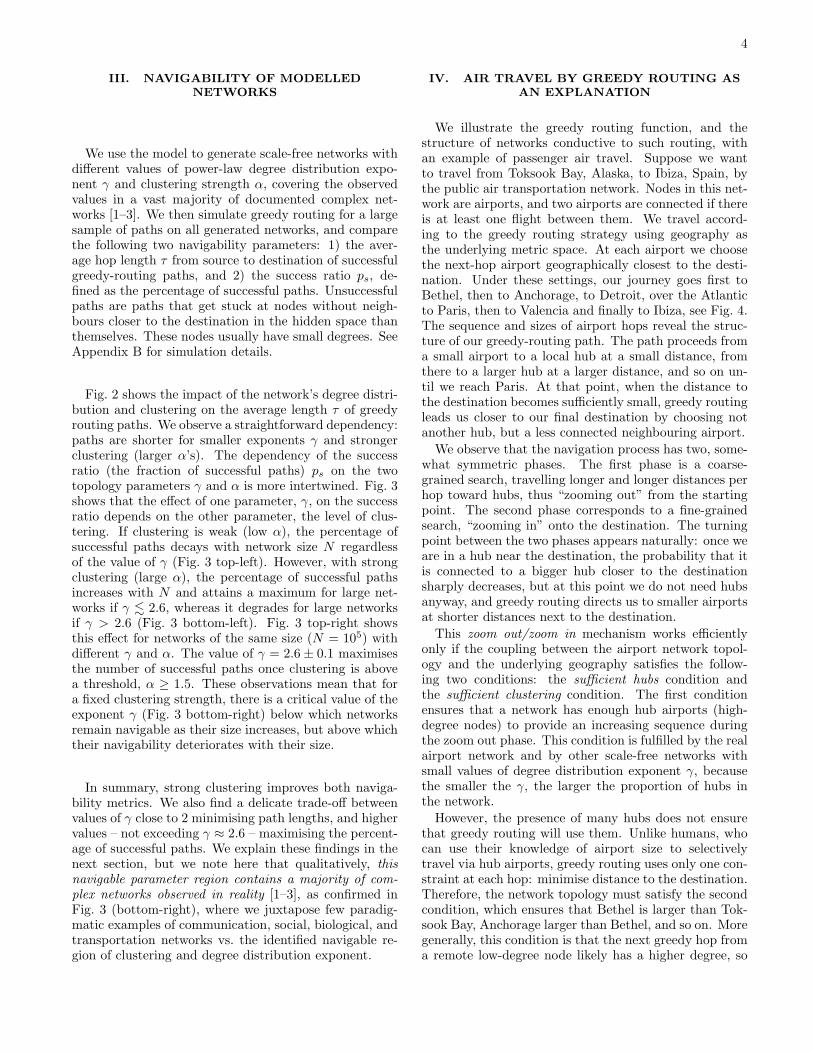
III. NAVIGABILITY OF MODELLEDNETWORKS

We use the model to generate scale-free networks withdifferent values of power-law degree distribution expo-nent γ and clustering strength α, covering the observedvalues in a vast majority of documented complex net-works [1–3]. We then simulate greedy routing for a largesample of paths on all generated networks, and comparethe following two navigability parameters: 1) the aver-age hop length τ from source to destination of successfulgreedy-routing paths, and 2) the success ratio ps, de-fined as the percentage of successful paths. Unsuccessfulpaths are paths that get stuck at nodes without neigh-bours closer to the destination in the hidden space thanthemselves. These nodes usually have small degrees. SeeAppendix B for simulation details.

Fig. 2 shows the impact of the network’s degree distri-bution and clustering on the average length τ of greedyrouting paths. We observe a straightforward dependency:paths are shorter for smaller exponents γ and strongerclustering (larger α’s). The dependency of the successratio (the fraction of successful paths) ps on the twotopology parameters γ and α is more intertwined. Fig. 3shows that the effect of one parameter, γ, on the successratio depends on the other parameter, the level of clus-tering. If clustering is weak (low α), the percentage ofsuccessful paths decays with network size N regardlessof the value of γ (Fig. 3 top-left). However, with strongclustering (large α), the percentage of successful pathsincreases with N and attains a maximum for large net-works if γ . 2.6, whereas it degrades for large networksif γ > 2.6 (Fig. 3 bottom-left). Fig. 3 top-right showsthis effect for networks of the same size (N = 105) withdifferent γ and α. The value of γ = 2.6± 0.1 maximisesthe number of successful paths once clustering is abovea threshold, α ≥ 1.5. These observations mean that fora fixed clustering strength, there is a critical value of theexponent γ (Fig. 3 bottom-right) below which networksremain navigable as their size increases, but above whichtheir navigability deteriorates with their size.

In summary, strong clustering improves both naviga-bility metrics. We also find a delicate trade-off betweenvalues of γ close to 2 minimising path lengths, and highervalues – not exceeding γ ≈ 2.6 – maximising the percent-age of successful paths. We explain these findings in thenext section, but we note here that qualitatively, thisnavigable parameter region contains a majority of com-plex networks observed in reality [1–3], as confirmed inFig. 3 (bottom-right), where we juxtapose few paradig-matic examples of communication, social, biological, andtransportation networks vs. the identified navigable re-gion of clustering and degree distribution exponent.

IV. AIR TRAVEL BY GREEDY ROUTING ASAN EXPLANATION

We illustrate the greedy routing function, and thestructure of networks conductive to such routing, withan example of passenger air travel. Suppose we wantto travel from Toksook Bay, Alaska, to Ibiza, Spain, bythe public air transportation network. Nodes in this net-work are airports, and two airports are connected if thereis at least one flight between them. We travel accord-ing to the greedy routing strategy using geography asthe underlying metric space. At each airport we choosethe next-hop airport geographically closest to the desti-nation. Under these settings, our journey goes first toBethel, then to Anchorage, to Detroit, over the Atlanticto Paris, then to Valencia and finally to Ibiza, see Fig. 4.The sequence and sizes of airport hops reveal the struc-ture of our greedy-routing path. The path proceeds froma small airport to a local hub at a small distance, fromthere to a larger hub at a larger distance, and so on un-til we reach Paris. At that point, when the distance tothe destination becomes sufficiently small, greedy routingleads us closer to our final destination by choosing notanother hub, but a less connected neighbouring airport.

We observe that the navigation process has two, some-what symmetric phases. The first phase is a coarse-grained search, travelling longer and longer distances perhop toward hubs, thus “zooming out” from the startingpoint. The second phase corresponds to a fine-grainedsearch, “zooming in” onto the destination. The turningpoint between the two phases appears naturally: once weare in a hub near the destination, the probability that itis connected to a bigger hub closer to the destinationsharply decreases, but at this point we do not need hubsanyway, and greedy routing directs us to smaller airportsat shorter distances next to the destination.

This zoom out/zoom in mechanism works efficientlyonly if the coupling between the airport network topol-ogy and the underlying geography satisfies the follow-ing two conditions: the sufficient hubs condition andthe sufficient clustering condition. The first conditionensures that a network has enough hub airports (high-degree nodes) to provide an increasing sequence duringthe zoom out phase. This condition is fulfilled by the realairport network and by other scale-free networks withsmall values of degree distribution exponent γ, becausethe smaller the γ, the larger the proportion of hubs inthe network.

However, the presence of many hubs does not ensurethat greedy routing will use them. Unlike humans, whocan use their knowledge of airport size to selectivelytravel via hub airports, greedy routing uses only one con-straint at each hop: minimise distance to the destination.Therefore, the network topology must satisfy the secondcondition, which ensures that Bethel is larger than Tok-sook Bay, Anchorage larger than Bethel, and so on. Moregenerally, this condition is that the next greedy hop froma remote low-degree node likely has a higher degree, so

5

0100020003000400050006000700080009000

Distance to Ibiza (Km)

0.5

1

1.5

2

2.5

3

Lo

ga

rith

m o

f a

irp

ort

de

gre

e

Toksook bay

Bethel

Anchorage

Detroit

Paris

Valencia

Ibiza

FIG. 4: Greedy-routing path from Toksook Bay to Ibiza. At each intermediate airport, the next hop is the airportclosest to Ibiza geographically. Sizes of symbols representing the airports are proportional to the logarithm of their degrees.The inset shows the changing distance to Ibiza (in the x axis) and the degree of the visited airports (y axis, in logarithmicscale).

that greedy paths typically head first toward the highlyconnected network core. But the network metric strengthis exactly the required property: preference for connec-tions between nodes nearby in the hidden space meansthat low-degree nodes are less likely to have connectivityto distant low-degree nodes; only high-degree nodes canhave long-range connection that greedy routing will ef-fectively select. The stronger this coupling between themetric space and topology (the higher α in Eq. (1)), thestronger the clustering in the network.

To illustrate, imagine an airport network without suf-ficient clustering, one where the airport closest to ourdestination (Ibiza) among all airports connected to ourcurrent node (Toksook Bay, Alaska) is not Bethel, whichis bigger than Toksook Bay, but Nightmute, Alaska, anearby airport of comparable size to Toksook Bay. Asgreedy routing first leads us to Nightmute, then to an-other small nearby airport, and then to another, we canno longer get to Ibiza in few hops. Worse, travelling viathese numerous small airports, we could reach one withno connecting flights heading closer to Ibiza. Our greedyrouting would be stuck at this airport with an unsuccess-ful path.

These factors explain why the most navigable topolo-gies correspond to scale-free networks with small expo-nents of the degree distribution, i.e., a large number ofhubs, and with strong clustering, i.e., strong coupling be-tween the hidden geometry and the observed topology.

V. THE STRUCTURE OF GREEDY-ROUTINGPATHS

We observe the discussed zoom-out/zoom-in mecha-nism in analytical calculations and numerical simula-tions. Specifically, we calculate in Appendix C the prob-ability that the next hop from a node of degree k locatedat hidden distance d from the destination has a largerdegree k′ > k, in which case the path moves toward thehigh-degree network core, see Fig. 5. In the most navi-gable case, with small degree-distribution exponent andstrong clustering, the probability of increasing the nodedegree along the path is high at low-degree nodes, andsharply decreases to zero after reaching a node of a crit-ical degree value, which increases with distance d. Thisobservation implies that greedy-routing paths first prop-agate up to higher-degree nodes in the network core andthen exit the core toward low-degree destinations in theperiphery. In contrast, with low clustering, paths areless likely to find higher-degree nodes regardless of thedistance to the destination. This path structure violatesthe zoom-out/zoom-in pattern required for efficient nav-igation.

Fig. 6 shows the structure of greedy-routing pathsin simulations, further confirming our analysis. Weagain see that for small degree-distribution exponentsand strong clustering (upper left and middle left), therouting process quickly finds a way to the high-degreecore, makes a few hops there, and then descends to a low-degree destination. In the other, non-navigable cases, the

6

100

101

102

103

0

0.2

0.4

0.6

0.8

1P

up(k

,d)

100

101

102

103

0

0.2

0.4

0.6

0.8

1

100

101

102

103

0

0.2

0.4

0.6

0.8

1

Pup

(k,d

)

100

101

102

103

0

0.2

0.4

0.6

0.8

1

100

101

102

103

k

0

0.2

0.4

0.6

0.8

1

Pup

(k,d

)

100

101

102

103

k

0

0.2

0.4

0.6

0.8

1

d=100d=1000d=10000d=100000

α=5.0, γ=2.2

α=5.0, γ=2.5

α=5.0, γ=3.0

α=1.1, γ=2.2

α=1.1, γ=2.5

α=1.1, γ=3.0

FIG. 5: Probability that greedy routing travels tohigher-degree nodes. More precisely, the probabilityPup(k, d) that the greedy-routing next hop after a node ofdegree k located at distance d from a destination has higherdegree k′ ≥ k and is closer to the destination. The distancelegend in the right-bottom plot applies to all the plots. Theresults are for the large-graph limit N →∞.

process can almost never get to the core of high-degreenodes. Instead, it wanders in the low-degree peripheryincreasing the probability of getting lost at low-degreenodes.

VI. CONCLUSION

In this paper, we have shown that the existence ofhidden metric spaces, coupled with heterogeneous degreedistributions and strong clustering, explains the surpris-ing navigability of real networks. Discovery of the explicitstructure of such hidden metric spaces underlying actualnetworks may have profound practical implications. Insocial or some communication networks (e.g., the Web,overlay, or online social networks) hidden spaces wouldyield efficient strategies for searching specific individualsor content. The metric spaces hidden under some biolog-ical networks (such as neural, gene regulatory networks,or signalling pathways) can become a powerful tool instudying the structure of information or signal flows inthese networks. Even more promising and immediatelyapplicable is the potential use of hidden metric spacesin the global Internet. Its routing architecture bears

FIG. 6: The structure of greedy-routing paths. We vi-sualise the results of our simulation of greedy routing in mod-elled networks with different values of γ and α observed in realcomplex networks. The hidden distance between the startingpoint and the destination is always approximately 104, andthe network size N and number of attempted paths is always105 for each (γ, α) combination, but the number of successfulpaths and path hop-lengths vary, cf. Figs. 2,3. All paths startand end at low-degree nodes located, respectively, in the left-and right-bottom corners of the diagrams (see top left plot).For each (γ, α) we depict a single typical path in black anduse colour to indicate how often paths included a node of de-gree k located at distance d from the destination (blue/redindicates exponentially less/more visits to those nodes). Thesimulations confirm that only when γ is small and α is largedoes the average path structure follow the zoom-out/zoom-in pattern that characterises successful greedy routing in realnetworks, e.g., the airport network in our example.

long-standing scalability problems related to the need forrouters to maintain a coherent view of the increasinglydynamic and ever-growing global Internet topology [19].Greedy routing over the Internet’s hidden metric spacewould remove this scalability bottleneck, as it does notrequire any global topological awareness. In general, we

7

believe that the present and future work on hidden metricspaces and network navigability will deepen our under-standing of the fundamental laws describing relationshipsbetween structure and function of complex networks.

Acknowledgments

We thank M. Angeles Serrano for useful comments anddiscussions. This work was supported in part by DGESgrants No. FIS2004-05923-CO2-02 and FIS2007-66485-C02-02, Generalitat de Catalunya grant No. SGR00889,the Ramon y Cajal program of the Spanish Ministry ofScience, and by NSF CNS-0434996 and CNS-0722070, byDHS N66001-08-C-2029, and by Cisco Systems.

APPENDIX A: A MODEL WITH THE CIRCLEAS A HIDDEN METRIC SPACE

In our model we place all nodes on a circle by assign-ing them a random variable θ, i.e., their polar angle, dis-tributed uniformly in [0, 2π). The circle radius R growslinearly with the total number of nodes N , 2πR = N ,in order to keep the average density of nodes on the cir-cle fixed to 1. We next assign to each node its expecteddegree κ drawn from some distribution ρ(κ). The con-nection probability between two nodes with hidden co-ordinates (θ, κ) and (θ′, κ′) takes the form

r(θ, κ; θ′, κ′) =(

1 +d(θ, θ′)µκκ′

)−α, µ =

(α− 1)2〈k〉

, (A1)

where d(θ, θ′) is the geodesic distance between the twonode on the circle, while 〈k〉 is the average degree. Onecan show that the average degree of nodes with hiddenvariable κ, k(κ), is proportional to κ.[20] This pro-portionality guarantees that the shape of the node de-gree distribution P (k) in generated networks is approx-imately the same as the shape of ρ(κ). The choice ofρ(κ) = (γ − 1)κγ−1

0 κ−γ , κ > κ0 ≡ (γ − 2)〈k〉/(γ − 1),γ > 2, generates random networks with a power-law de-gree distribution of the form P (k) ∼ k−γ .

APPENDIX B: NUMERICAL SIMULATIONS

Our model has three independent parameters: ex-ponent γ of power-law degree distributions, clusteringstrength α, and average degree 〈k〉. We fix the latter to6, which is roughly equal to the average degree of somereal networks of interest [13, 14], and vary γ ∈ [2.1, 3]and α ∈ [1.1, 5], covering their observed ranges in docu-mented complex networks [1–3]. For each (γ, α) pair, weproduce networks of different sizes N ∈ [103, 105] gener-ating, for each (γ, α,N), a number of different networkinstances—from 40 for large N to 4000 for small N . In

each network instance G, we randomly select 106 source-destination pairs (a, b) and execute the greedy-routingprocess for them starting at a and selecting, at each hoph, the next hop as the h’s neighbour in G closest to bin the circle. If for a given (a, b), this process visits thesame node twice, then the corresponding path leads to aloop and is unsuccessful. We then average the measuredvalues of path hop lengths τ and percentage of successfulpaths ps across all pairs (a, b) and networks G for thesame (γ, α,N).

APPENDIX C: THE ONE-HOP PROPAGATOROF GREEDY ROUTING

To derive the greedy-routing propagator in this ap-pendix, we adopt a slightly more general formalism thanin the main text. Specifically, we assume that nodeslive in a generic metric space H and, at the same time,have intrinsic attributes unrelated to H. Contrary tonormed spaces or Riemannian manifolds, generic metricspaces do not admit any coordinates, but we still use thecoordinate-based notations here to simplify the exposi-tion below, and denote by x nodes’ coordinates in H andby ω all their other, non-geometric attributes. In otherwords, hidden variables x and ω in this general formal-ism represent some collections of nodes’ geometric andnon-geometric hidden attributes, not just a pair of scalarquantities. Therefore, integrations over x and ω in whatfollows stand merely to denote an appropriate form ofsummation in each concrete case.

As in the main text, we assume that x and ω are inde-pendent random variables so that the probability densityto find a node with hidden variables (x, ω) is

ρ(x, ω) = δ(x)ρ(ω)/N, (C1)

where ρ(ω) is the probability density of the ω variablesand δ(x) is the concentration of nodes in H. The totalnumber of nodes is

N =∫Hδ(x)dx, (C2)

and the connection probability between two nodes is anintegrable decreasing function of the hidden distance be-tween them,

r(x, ω; x′, ω′) = r[d(x,x′)/dc(ω, ω′)], (C3)

where dc(ω, ω′) a characteristic distance scale that de-pends on ω and ω′.

We define the one-step propagator of greedy routing asthe probability G(x′, ω′|x, ω; xt) that the next hop aftera node with hidden variables (x, ω) is a node with hid-den variables (x′, ω′), given that the final destination islocated at xt.

To further simplify the notations below, we label theset of variables (x, ω) as a generic hidden variable h and

8

undo this notation change at the end of the calculationsaccording to the following rules:

(x, ω) −→ hρ(x, ω) −→ ρ(h)dxdω −→ dh

r(x, ω; x′, ω′) −→ r(h, h′).

(C4)

We begin the propagator derivation assuming that aparticular network instance has a configuration given

by {h, ht, h1, · · · , hN−2} ≡ {h, ht; {hj}} with j =1, · · · , N − 2, where h and ht denote the hidden vari-ables of the current hop and the destination, respectively.In this particular network configuration, the probabilitythat the current node’s next hop is a particular node iwith hidden variable hi is the probability that the cur-rent node is connected to i but disconnected to all nodesthat are closer to the destination than i,

Prob(i|h, ht; {hj}) = r(h, hi)N−2∏

j(6=i)=1

[1− r(h, hj)]Θ[d(hi,ht)−d(hj ,ht)] , (C5)

where Θ(·) is the Heaviside step function. Tak-ing the average over all possible configurations{h1, · · · , hi−1, hi+1, · · · , hN−2} excluding node i, we ob-tain

Prob(i|h, ht;hi) = r(h, hi)(

1− 1N − 3

k(h|hi, ht))N−3

,

(C6)where

k(h|hi, ht) = (N − 3)∫d(hi,ht)<d(h′,ht)

ρ(h′)r(h, h′)dh′

(C7)is the average number of connections between the currentnode and nodes closer to the destination than node i,excluding i and t.

The probability that the next hop has hidden variableh′, regardless of its label, i.e., index i, is

Prob(h′|h, ht) =N−2∑i=1

ρ(h′)Prob(i|h, ht;h′). (C8)

In the case of sparse networks, k(h|h′, ht) is a finite quan-

tity. Taking the limit of large N , the above expressionsimplifies to

Prob(h′|h, ht) = Nρ(h′)r(h, h′)e−k(h|h′,ht). (C9)

Yet, this equation is not a properly normalized probabil-ity density function for the variable h′ since node h canhave degree zero with some probability. If we consideronly nodes with degrees greater than zero, then the nor-malization factor is given by 1 − e−k(h). Therefore, theproperly normalized propagator is finally

G(h′|h, ht) =Nρ(h′)r(h, h′)e−k(h|h′,ht)

1− e−k(h). (C10)

We now undo the notation change and express thispropagator in terms of our mixed coordinates:

G(x′, ω′|x, ω; xt) =δ(x′)ρ(ω′)

1− e−k(x,ω)r

[d(x,x′)dc(ω, ω′)

]e−k(x,ω|x′,xt),

(C11)with

k(x, ω|x′,xt) =∫d(x′,xt)>d(y,xt)

dy∫dω′δ(y)ρ(ω′)r

[d(x,y)dc(ω, ω′)

]. (C12)

In the particular case of the S1 model, we can expressthis propagator in terms of relative hidden distances in-stead of absolute coordinates. Namely, G(d′, ω′|d, ω) isthe probability that an ω-labeled node at hidden distance

d from the destination has as the next hop an ω′-labelednode at hidden distance d′ from the destination. Aftertedious calculations, the resulting expression reads:

9

G(d′, ω′|d, ω) =

(γ−1)ω′γ

[1

(1+ d−d′κωω′ )

α+ 1

(1+ d+d′κωω′ )

α

]exp

{(1−γ)κωα−1

[B(d−d

′

κω , γ − 2, 2− α)− B(d+d′

κω , γ − 2, 2− α)]}

; d′ ≤ d

(γ−1)ω′γ

[1

(1+ d′−dκωω′ )

α+ 1

(1+ d+d′κωω′ )

α

]exp

{(1−γ)κωα−1

[2

γ−2 − B(d′−dκω , γ − 2, 2− α)− B(d+d′

κω , γ − 2, 2− α)]}

; d′ > d

,

(C13)

10-3 10-2 10-1 100 101 102

ω/d1/20

0.2

0.4

0.6

0.8

1

P up(ω

,d)

10-3 10-2 10-1 100 101 102

ω/d1/20

0.2

0.4

0.6

0.8

1

P up(ω

,d)

10-3 10-2 10-1 100 101 102

ω/d1/20

0.2

0.4

0.6

0.8

1

P up(ω

,d)

10-3 10-2 10-1 100 101 102

ω/d1/20

0.2

0.4

0.6

0.8

1

P up(ω

,d)

10-3 10-2 10-1 100 101 102

ω/d1/20

0.2

0.4

0.6

0.8

1

P up(ω

,d)

10-3 10-2 10-1 100 101 102

ω/d1/20

0.2

0.4

0.6

0.8

1

P up(ω

,d)

d=100d=1000d=10000d=100000

α=5.0, γ=2.2

α=5.0, γ=2.5

α=5.0, γ=3.0

α=1.1, γ=2.2

α=1.1, γ=2.5

α=1.1, γ=3.0

FIG. 7: Probability Pup(ω/d1/2, d).

where we have defined function

B(z, a, b) ≡ z−a∫ z

0

ta−1(1 + t)b−1dt, (C14)

which is somewhat similar to the incomplete beta func-tion B(z, a, b) =

∫ z0ta−1(1− t)b−1dt.

One of the informative quantities elucidating the struc-ture of greedy-routing paths is the probability Pup(ω, d)that the next hop after an ω-labeled node at distance dfrom the destination has a higher value of ω. The greedy-routing propagator defines this probability as

Pup(ω, d) =∫ω′≥ω

dω′∫d′<d

dd′G(d′, ω′|d, ω), (C15)

and we show Pup(ω/d1/2, d) in Fig. 7. We see that theproper scaling of ωc ∼ d1/2, where ωc is the criticalvalue of ω above which Pup(ω, d) quickly drops to zero,is present only when clustering is strong. Furthermore,Pup(ω, d) is an increasing function of ω for small ω’s onlywhen the degree distribution exponent γ is close to 2.A combination of these two effects guarantees that thelayout of greedy routes properly adapts to increasing dis-tances or graph sizes, thus making networks with strongclustering and γ’s greater than but close to 2 navigable.

[1] R. Albert and A.-L. Barabasi, Rev. Mod. Phys. 74, 47(2002).

[2] M. E. J. Newman, SIAM Rev 45, 167 (2003).[3] S. N. Dorogovtsev and J. F. F. Mendes, Evolution of

networks: From biological nets to the Internet and WWW(Oxford University Press, Oxford, 2003).

[4] S. Boccaletti, V. Latora, Y. Moreno, M. Chavez, and D.-U. Hwang, Phys. Rep. 424, 175 (2006).

[5] M. Castells, The rise of the network society (BlackwellPublishing, Oxford, 1996).

[6] R. Pastor-Satorras and A. Vespignani, Evolution andStructure of the Internet. A Statistical Physics Approach(Cambridge University Press, Cambridge, 2004).

[7] D. J. Watts, P. S. Dodds, and M. E. J. Newman, Science296, 1302 (2002).

[8] M. Girvan and M. E. J. Newman, Proc Natl Acad SciUSA 99, 7821 (2002).

[9] F. Menczer, Proc Natl Acad Sci USA 99, 14014 (2002).[10] E. A. Leicht, P. Holme, and M. E. J. Newman, Phys Rev

E 73, 026120 (2006).[11] M. A. Serrano, D. Krioukov, and M. Boguna, Phys. Rev.

Lett. p. (in press) (2008).[12] D. J. Watts and S. H. Strogatz, Nature 393, 440 (1998).[13] P. Mahadevan, D. Krioukov, M. Fomenkov, B. Huffaker,

X. Dimitropoulos, kc claffy, and A. Vahdat, ComputCommun Rev 36, 17 (2006).

[14] M. Boguna, R. Pastor-Satorras, A. Dıaz-Guilera, andA. Arenas, Phys Rev E 70, 056122 (2004).

[15] H. Jeong, B. Tombor, R. Albert, Z. N. Oltvai, and A.-L.Barabasi, Nature 407, 651 (2000).

[16] A. Barrat, M. Barthelemy, R. Pastor-Satorras, andA. Vespignani, Proc. Natl. Acad. Sci. USA 101, 3747(2004).

[17] S. Milgram, Psychol Today 1, 61 (1967).[18] J. Kleinberg, Nature 406, 845 (2000).[19] D. Meyer, L. Zhang, and K. Fall, eds., Report from the

IAB Workshop on Routing and Addressing (The InternetArchitecture Board, 2007).

10

[20] M. Boguna and R. Pastor-Satorras, Phys. Rev. E 68,036112 (2003).

[21] J. M. Guiot, Eur J of Soc Psychol 6, 503 (1976).[22] The percentage of successfully delivered messages in

the original experiments was around 30% [17], whiletheir subsequent simple modifications improved it up to90% [21].