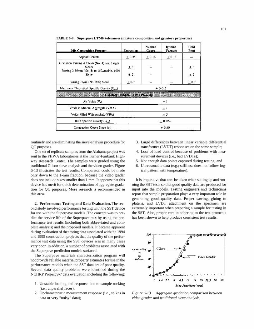
N ATIONAL C OOPERATIVE H IGHWAY R ESEARCH P ROGRAM NCHRP Report 409 Quality Control and Acceptance of Superpave-Designed Hot Mix Asphalt Transportation Research Board National Research Council
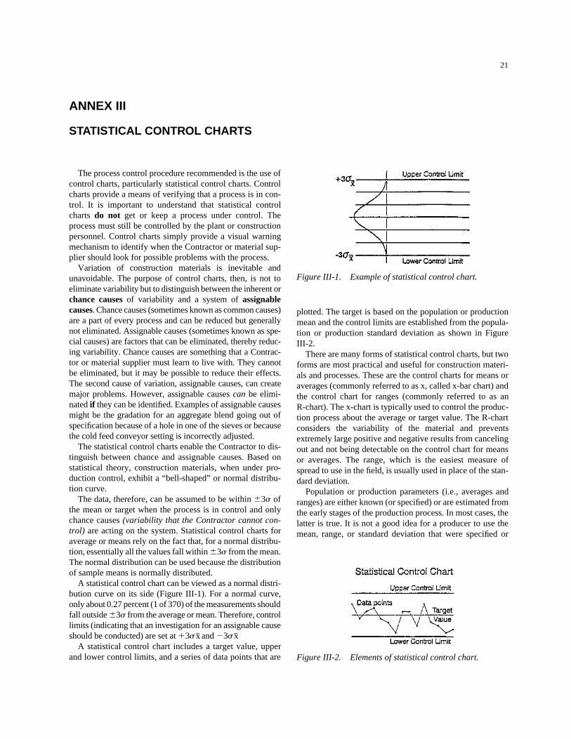
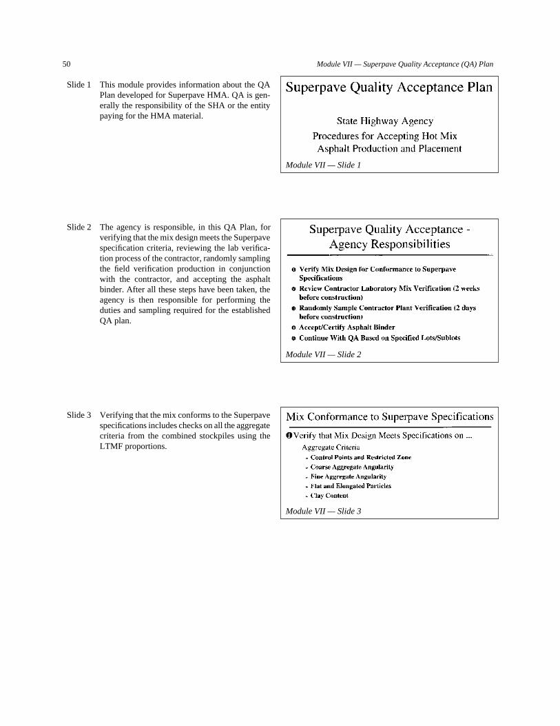
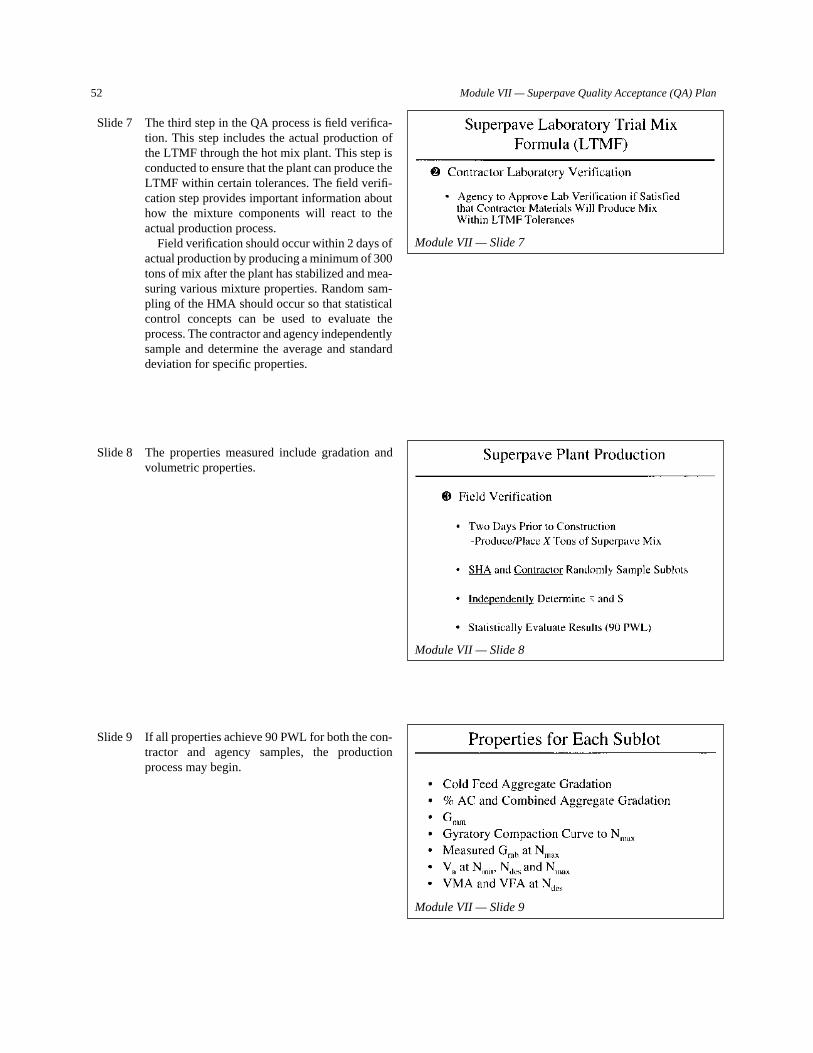
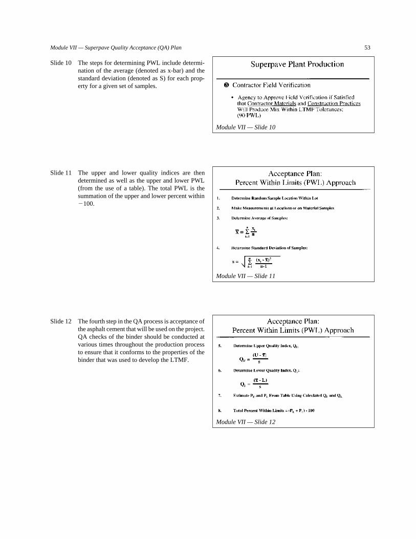
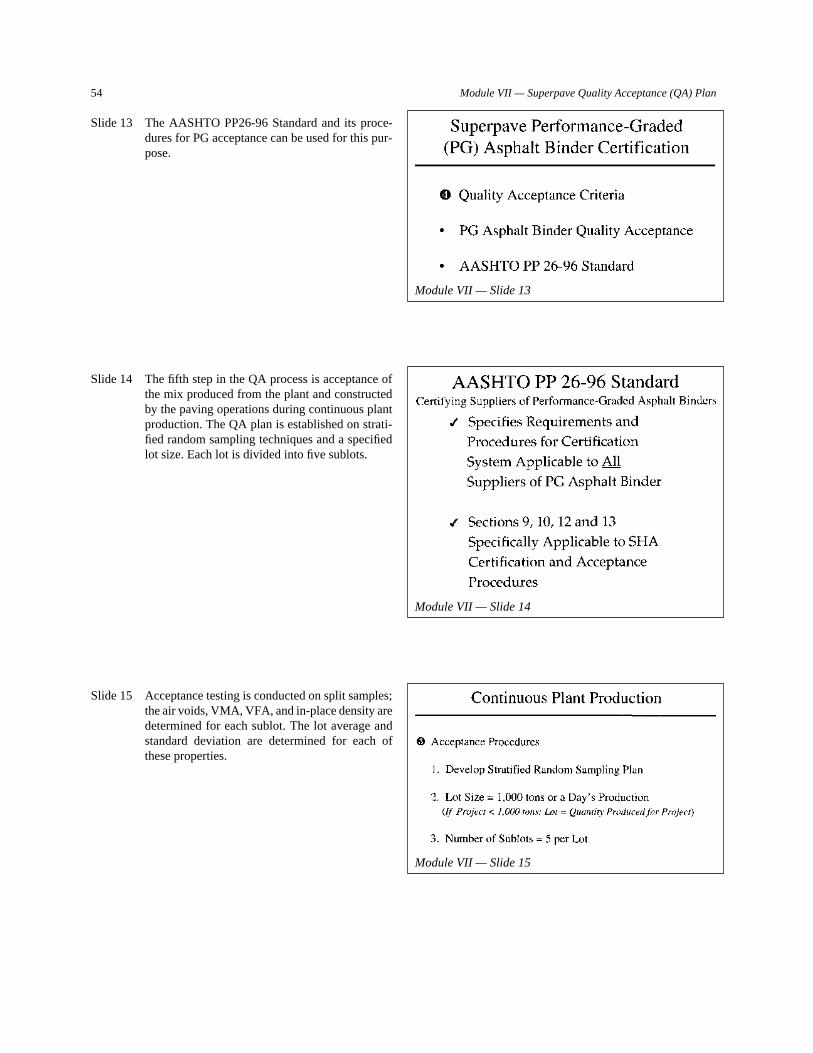
Transcript
N A T I O N A L C O O P E R A T I V E H I G H W A Y R E S E A R C H P R O G R A M
NCHRP Report 409
Quality Control and Acceptance ofSuperpave-Designed Hot Mix Asphalt
Transportation Research BoardNational Research Council
W. M. LACKEY, Kansas Department of Transportation (Chair)
TIMOTHY B. ASCHENBRENER, Colorado Department of Transportation
WAYNE BRULE, New York State Department of Transportation
JOHN D’ANGELO, Federal Highway Administration
GAIL JENSEN, Mathy Construction, Onalasha, WI
GALE C. PAGE, Florida Department of Transportation
CHARLES F. POTTS, APAC, Inc., Atlanta, GA
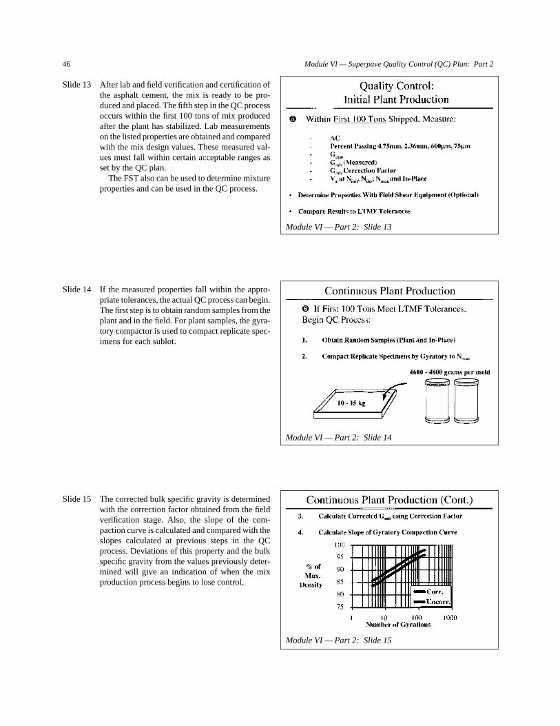
B. F. TEMPLETON, Texas Department of Transportation
JAMES M. WARREN, Asphalt Contractors Association of Florida, Inc.
PETER A. KOPAC, FHWA Liaison Representative
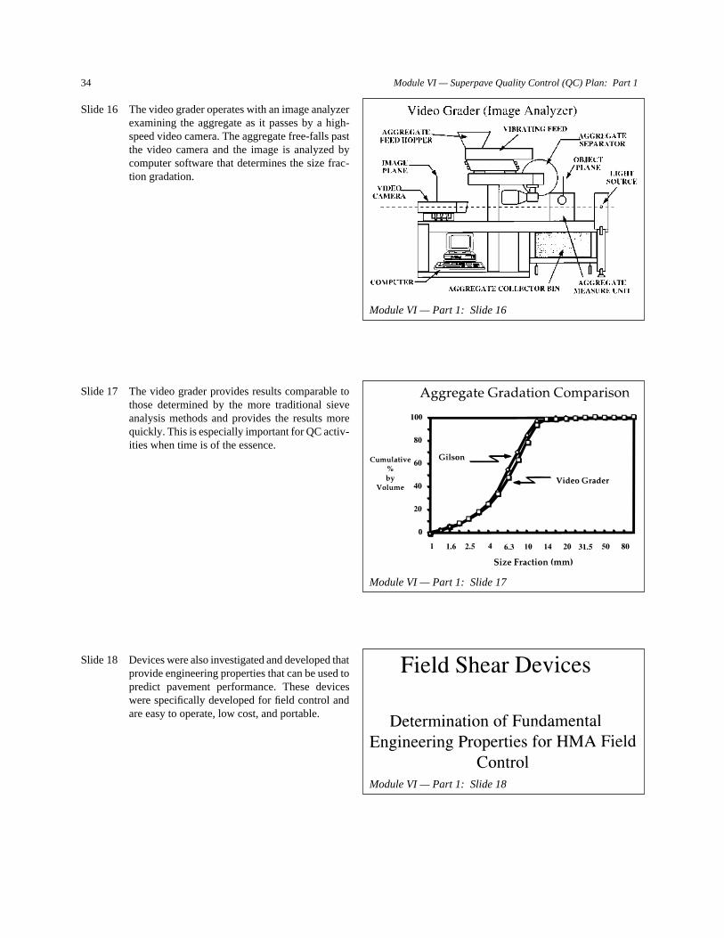
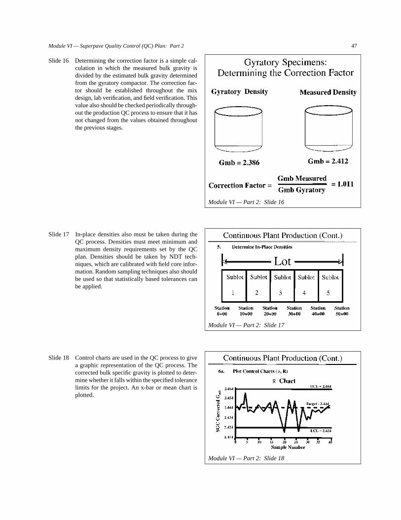
HALEEM TAHIR, AASHTO Liaison Representative
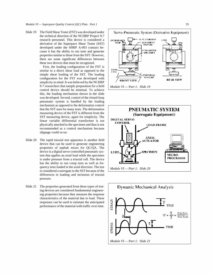
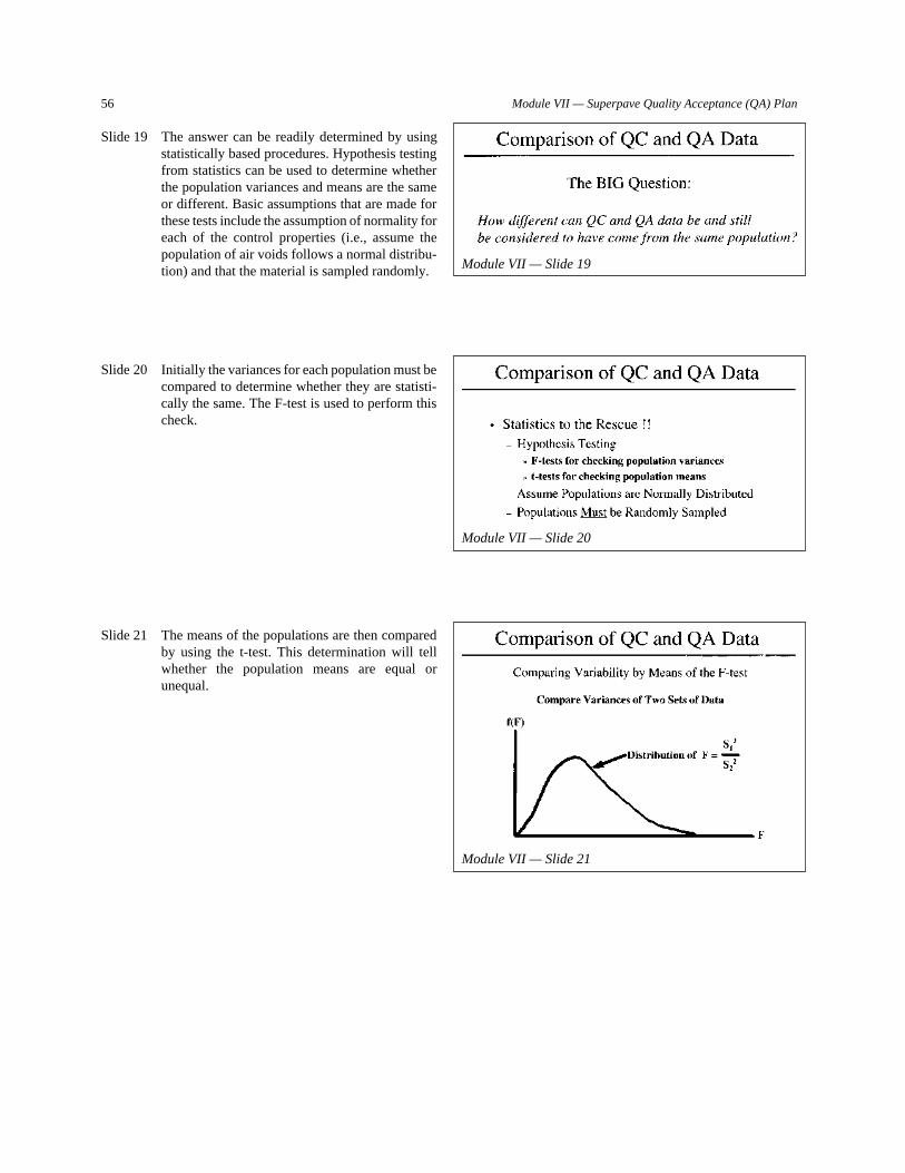
FRED HEJL, TRB Liaison Representative
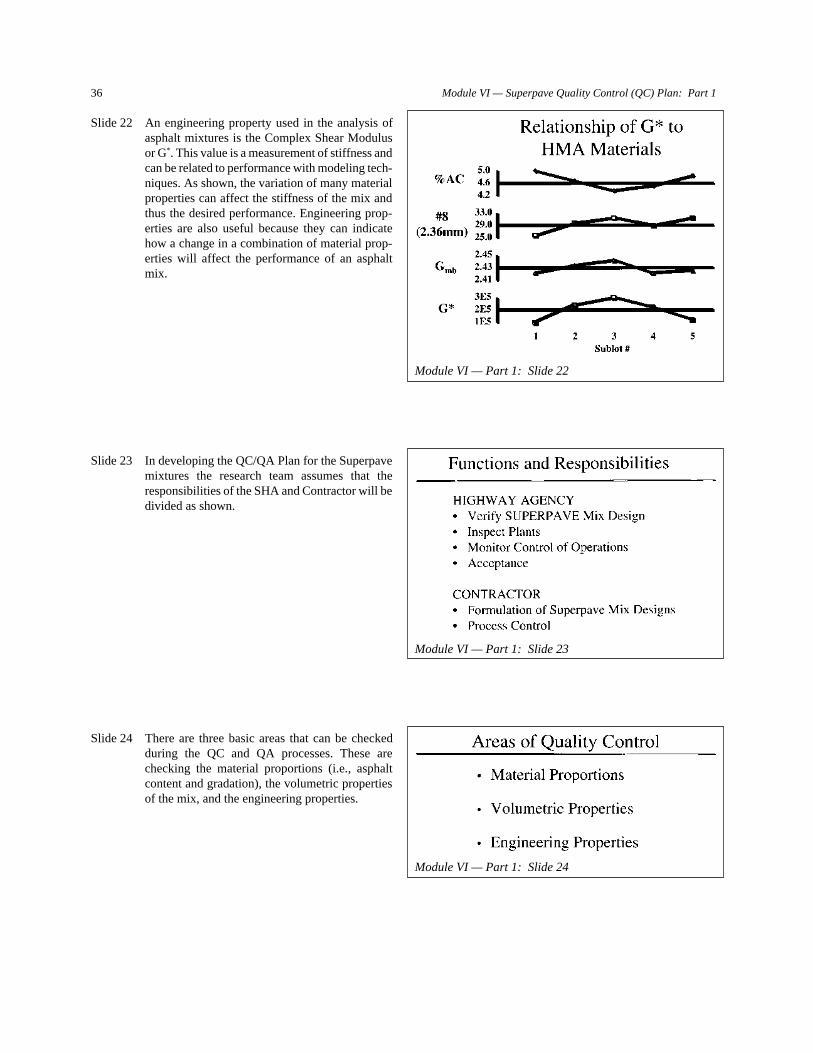
Project Panel D9-7 Field of Materials and Construction Area of Bituminous Materials
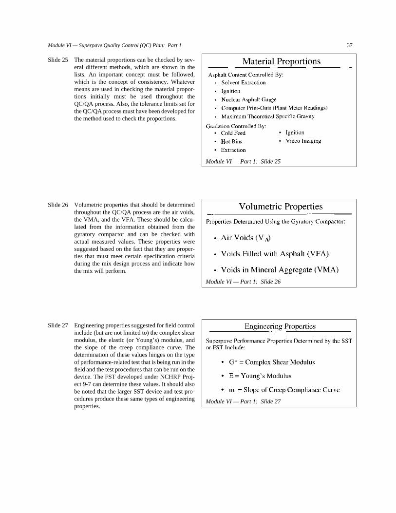
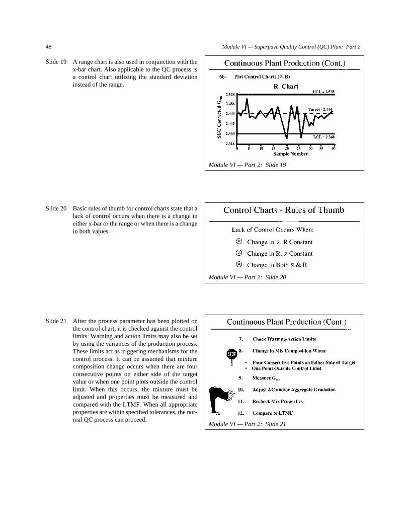
Program Staff
ROBERT J. REILLY, Director, Cooperative Research Programs
CRAWFORD F. JENCKS, Manager, NCHRP
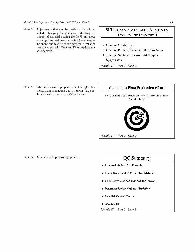
DAVID B. BEAL, Senior Program Officer
LLOYD R. CROWTHER, Senior Program Officer
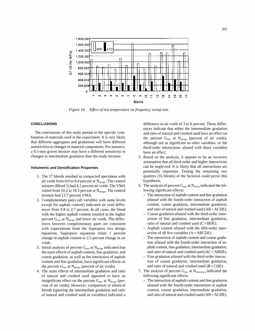
B. RAY DERR, Senior Program Officer
AMIR N. HANNA, Senior Program Officer
EDWARD T. HARRIGAN, Senior Program Officer
RONALD D. McCREADY, Senior Program Officer
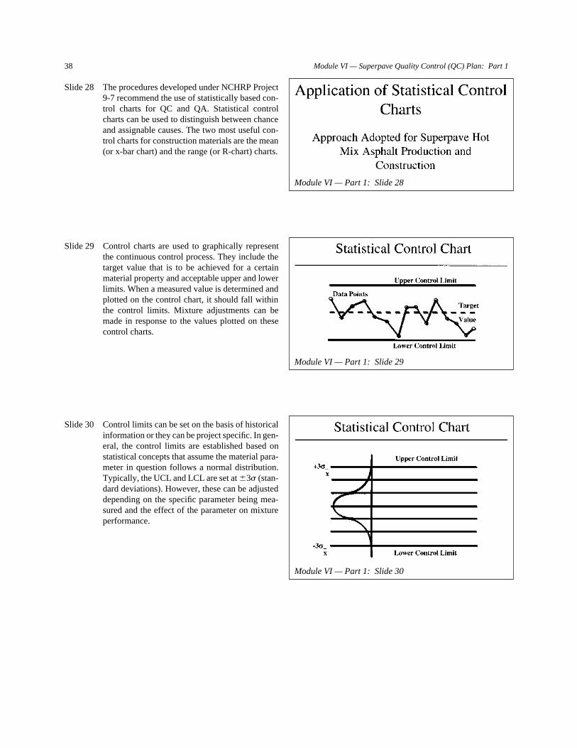
KENNETH S. OPIELA, Senior Program Officer
EILEEN P. DELANEY, Managing Editor
HELEN CHIN, Assistant Editor
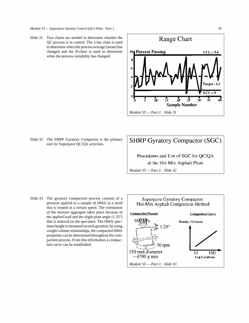
JAMIE FEAR, Assistant Editor
HILARY FREER, Assistant Editor
TRANSPORTATION RESEARCH BOARD EXECUTIVE COMMITTEE 1998
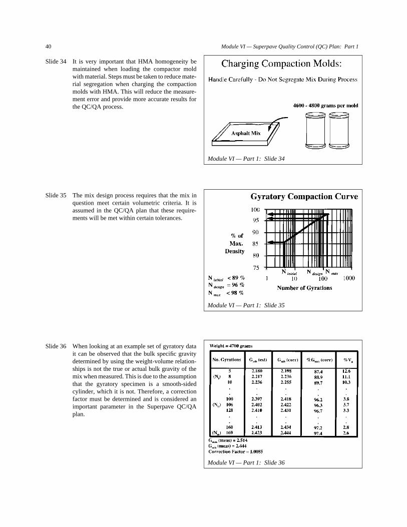
OFFICERSChairwoman: Sharon D. Banks, General Manager, AC Transit
Vice Chairman: Wayne Shackelford, Commissioner, Georgia Department of Transportation
Executive Director: Robert E. Skinner, Jr., Transportation Research Board
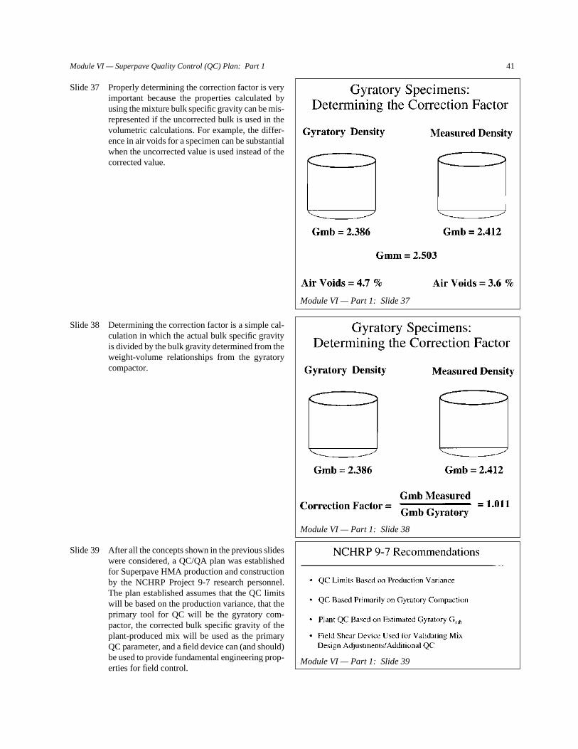
MEMBERSTHOMAS F. BARRY, JR., Secretary of Transportation, Florida Department of Transportation
BRIAN J. L. BERRY, Lloyd Viel Berkner Regental Professor, Bruton Center for Development Studies, University of Texas at Dallas
SARAH C. CAMPBELL, President, TransManagement, Inc., Washington, DC
E. DEAN CARLSON, Secretary, Kansas Department of Transportation
JOANNE F. CASEY, President, Intermodal Association of North America, Greenbelt, MD
JOHN W. FISHER, Director, ATLSS Engineering Research Center, Lehigh University
GORMAN GILBERT, Director, Institute for Transportation Research and Education, North Carolina State University
DELON HAMPTON, Chair and CEO, Delon Hampton & Associates, Washington, DC
LESTER A. HOEL, Hamilton Professor, Civil Engineering, University of Virginia
JAMES L. LAMMIE, Director, Parsons Brinckerhoff, Inc., New York, NY
THOMAS F. LARWIN, General Manager, San Diego Metropolitan Transit Development Board
BRADLEY L. MALLORY, Secretary of Transportation, Pennsylvania Department of Transportation
JEFFREY J. McCAIG, President and CEO, Trimac Corporation, Calgary, Alberta, Canada
JOSEPH A. MICKES, Chief Engineer, Missouri Department of Transportation
MARSHALL W. MOORE, Director, North Dakota Department of Transportation
ANDREA RINIKER, Executive Director, Port of Tacoma
JOHN M. SAMUELS, VP-Operations Planning & Budget, Norfolk Southern Corporation, Norfolk, VA
LES STERMAN, Executive Director, East-West Gateway Coordinating Council, St. Louis, MO
JAMES W. VAN LOBEN SELS, Director, CALTRANS (Past Chair, 1996)
MARTIN WACHS, Director, University of California Transportation Center, University of California at Berkeley
DAVID L. WINSTEAD, Secretary, Maryland Department of Transportation
DAVID N. WORMLEY, Dean of Engineering, Pennsylvania State University (Past Chair, 1997)
MIKE ACOTT, President, National Asphalt Pavement Association (ex officio)
JOE N. BALLARD, Chief of Engineers and Commander, U.S. Army Corps of Engineers (ex officio)
ANDREW H. CARD, JR., President and CEO, American Automobile Manufacturers Association (ex officio)
KELLEY S. COYNER, Acting Administrator, Research and Special Programs, U.S. Department of Transportation (ex officio)
MORTIMER L. DOWNEY, Deputy Secretary, Office of the Secretary, U.S. Department of Transportation (ex officio)
FRANCIS B. FRANCOIS, Executive Director, American Association of State Highway and Transportation Officials (ex officio)
DAVID GARDINER, Assistant Administrator, U.S. Environmental Protection Agency (ex officio)
JANE F. GARVEY, Federal Aviation Administrator, U.S. Department of Transportation (ex officio)
JOHN E. GRAYKOWSKI, Acting Maritime Administrator, U.S. Department of Transportation (ex officio)
ROBERT A. KNISELY, Deputy Director, Bureau of Transportation Statistics, U.S. Department of Transportation (ex officio)
GORDON J. LINTON, Federal Transit Administrator, U.S. Department of Transportation (ex officio)
RICARDO MARTINEZ, National Highway Traffic Safety Administrator, U.S. Department of Transportation (ex officio)
WALTER B. McCORMICK, President and CEO, American Trucking Associations, Inc. (ex officio)
WILLIAM W. MILLAR, President, American Public Transit Association (ex officio)
JOLENE M. MOLITORIS, Federal Railroad Administrator, U.S. Department of Transportation (ex officio)
KAREN BORLAUG PHILLIPS, Senior Vice President, Association of American Railroads (ex officio)
VALENTIN J. RIVA, President, American Concrete Pavement Association
GEORGE D. WARRINGTON, Acting President and CEO, National Railroad Passenger Corporation (ex officio)
KENNETH R. WYKLE, Federal Highway Administrator, U.S. Department of Transportation (ex officio)
NATIONAL COOPERATIVE HIGHWAY RESEARCH PROGRAMTransportation Research Board Executive Committee Subcommittee for NCHRP
SHARON BANKS, AC Transit (Chairwoman)
FRANCIS B. FRANCOIS, American Association of State Highway and
Transportation Officials
LESTER A. HOEL, University of Virginia
WAYNE SHACKELFORD, Georgia Department of Transportation
ROBERT E. SKINNER, JR., Transportation Research Board
DAVID N. WORMLEY, Pennsylvania State University
KENNETH R. WYKLE, Federal Highway Administration
N A T I O N A L C O O P E R A T I V E H I G H W A Y R E S E A R C H P R O G R A M
Report 409
Quality Control and Acceptance ofSuperpave-Designed Hot Mix Asphalt
RONALD J. COMINSKYand
BRIAN M. KILLINGSWORTHBrent Rauhut Engineering Inc.
Austin, TX
R. MICHAEL ANDERSONThe Asphalt Institute
Lexington, KY
DAVID A. ANDERSONPennsylvania Transportation Institute
Pennsylvania State University
WILLIAM W. CROCKFORDConsultant
College Station, TX
Subject Areas
Materials and Construction
T R A N S P O R T A T I O N R E S E A R C H B O A R D
NATIONAL RESEARCH COUNCIL
NATIONAL ACADEMY PRESSWashington, D.C. 1998
Research Sponsored by the American Association of State Highway and Transportation Officials in Cooperation with the
Federal Highway Administration
NATIONAL COOPERATIVE HIGHWAY RESEARCH PROGRAM
Systematic, well-designed research provides the most effectiveapproach to the solution of many problems facing highwayadministrators and engineers. Often, highway problems are of localinterest and can best be studied by highway departmentsindividually or in cooperation with their state universities andothers. However, the accelerating growth of highway transportationdevelops increasingly complex problems of wide interest tohighway authorities. These problems are best studied through acoordinated program of cooperative research.
In recognition of these needs, the highway administrators of theAmerican Association of State Highway and TransportationOfficials initiated in 1962 an objective national highway researchprogram employing modern scientific techniques. This program issupported on a continuing basis by funds from participatingmember states of the Association and it receives the full cooperationand support of the Federal Highway Administration, United StatesDepartment of Transportation.
The Transportation Research Board of the National ResearchCouncil was requested by the Association to administer the researchprogram because of the Board’s recognized objectivity andunderstanding of modern research practices. The Board is uniquelysuited for this purpose as it maintains an extensive committeestructure from which authorities on any highway transportationsubject may be drawn; it possesses avenues of communications andcooperation with federal, state and local governmental agencies,universities, and industry; its relationship to the National ResearchCouncil is an insurance of objectivity; it maintains a full-timeresearch correlation staff of specialists in highway transportationmatters to bring the findings of research directly to those who are ina position to use them.
The program is developed on the basis of research needsidentified by chief administrators of the highway and transportationdepartments and by committees of AASHTO. Each year, specificareas of research needs to be included in the program are proposedto the National Research Council and the Board by the AmericanAssociation of State Highway and Transportation Officials.Research projects to fulfill these needs are defined by the Board, andqualified research agencies are selected from those that havesubmitted proposals. Administration and surveillance of researchcontracts are the responsibilities of the National Research Counciland the Transportation Research Board.
The needs for highway research are many, and the NationalCooperative Highway Research Program can make significantcontributions to the solution of highway transportation problems ofmutual concern to many responsible groups. The program,however, is intended to complement rather than to substitute for orduplicate other highway research programs.
Published reports of the
NATIONAL COOPERATIVE HIGHWAY RESEARCH PROGRAM
are available from:
Transportation Research BoardNational Research Council2101 Constitution Avenue, N.W.Washington, D.C. 20418
and can be ordered through the Internet at:
http://www.nas.edu/trb/index.html
Printed in the United States of America
NATIONAL COOPERATIVE HIGHWAY RESEARCH PROGRAM
Systematic, well-designed research provides the most effectiveapproach to the solution of many problems facing highwayadministrators and engineers. Often, highway problems are of localinterest and can best be studied by highway departmentsindividually or in cooperation with their state universities andothers. However, the accelerating growth of highway transportationdevelops increasingly complex problems of wide interest tohighway authorities. These problems are best studied through acoordinated program of cooperative research.
In recognition of these needs, the highway administrators of theAmerican Association of State Highway and TransportationOfficials initiated in 1962 an objective national highway researchprogram employing modern scientific techniques. This program issupported on a continuing basis by funds from participatingmember states of the Association and it receives the full cooperationand support of the Federal Highway Administration, United StatesDepartment of Transportation.
The Transportation Research Board of the National ResearchCouncil was requested by the Association to administer the researchprogram because of the Board’s recognized objectivity andunderstanding of modern research practices. The Board is uniquelysuited for this purpose as it maintains an extensive committeestructure from which authorities on any highway transportationsubject may be drawn; it possesses avenues of communications andcooperation with federal, state and local governmental agencies,universities, and industry; its relationship to the National ResearchCouncil is an insurance of objectivity; it maintains a full-timeresearch correlation staff of specialists in highway transportationmatters to bring the findings of research directly to those who are ina position to use them.
The program is developed on the basis of research needsidentified by chief administrators of the highway and transportationdepartments and by committees of AASHTO. Each year, specificareas of research needs to be included in the program are proposedto the National Research Council and the Board by the AmericanAssociation of State Highway and Transportation Officials.Research projects to fulfill these needs are defined by the Board, andqualified research agencies are selected from those that havesubmitted proposals. Administration and surveillance of researchcontracts are the responsibilities of the National Research Counciland the Transportation Research Board.
The needs for highway research are many, and the NationalCooperative Highway Research Program can make significantcontributions to the solution of highway transportation problems ofmutual concern to many responsible groups. The program,however, is intended to complement rather than to substitute for orduplicate other highway research programs.
Note: The Transportation Research Board, the National Research Council,the Federal Highway Administration, the American Association of StateHighway and Transportation Officials, and the individual states participating inthe National Cooperative Highway Research Program do not endorse productsor manufacturers. Trade or manufacturers’ names appear herein solelybecause they are considered essential to the object of this report.
The project that is the subject of this report was a part of the National Cooperative
Highway Research Program conducted by the Transportation Research Board with the
approval of the Governing Board of the National Research Council. Such approval
reflects the Governing Board’s judgment that the program concerned is of national
importance and appropriate with respect to both the purposes and resources of the
National Research Council.
The members of the technical committee selected to monitor this project and to review
this report were chosen for recognized scholarly competence and with due
consideration for the balance of disciplines appropriate to the project. The opinions and
conclusions expressed or implied are those of the research agency that performed the
research, and, while they have been accepted as appropriate by the technical committee,
they are not necessarily those of the Transportation Research Board, the National
Research Council, the American Association of State Highway and Transportation
Officials, or the Federal Highway Administration, U.S. Department of Transportation.
Each report is reviewed and accepted for publication by the technical committee
according to procedures established and monitored by the Transportation Research
Board Executive Committee and the Governing Board of the National Research
Council.
FOREWORDBy Staff
Transportation ResearchBoard
This report presents a plan, in the form of a draft AASHTO standard practice, for qual-ity control (QC) and quality acceptance (QA) of field production, placement, and com-paction of hot mix asphalt (HMA) prepared in conformance with Superpave materials spec-ifications and mix designs. It will be of particular interest to materials engineers in statehighway agencies and to those agency and contractor personnel responsible for control andacceptance of HMA paving projects. The report also contains the detailed research resultssupporting the development of the QC/QA plan, including experimental data obtained dur-ing the construction of pavement projects using Superpave mix designs across the UnitedStates.
A principal product of the Strategic Highway Research Program (SHRP) is the Super-pave performance-based mix design and analysis method. This method incorporates new,performance-based material specifications, test methods, and design and analysis proce-dures for HMA. Interest in the Superpave method has grown rapidly since the conclusionof SHRP in 1993. The Superpave Lead State Team of the AASHTO Task Force on theImplementation of SHRP reported that in 1996, 28 states incorporated both binder and mixspecifications in awarding 95 Superpave projects. Nationally, these projects representedapproximately 1 percent of total projects and 2 percent of total tonnage. For 1997, projectedfigures indicated that the number of states using Superpave would increase to greater than40, while planned projects totaled in excess of 300. However, to realize the maximum ben-efit of improved performance possible through the Superpave method, state highway agen-cies must ensure that the production, placement, and compaction of HMA in field projectsare controlled to maintain compliance with the Superpave specifications and mix design.
Under NCHRP Project 9-7 “Field Procedures and Equipment to Implement SHRPAsphalt Specifications” Brent Rauhut Engineering Inc. was assigned the tasks of (1) estab-lishing comprehensive procedures and, if required, developing equipment for QC/QA offield production, placement, and compaction to ensure that as-placed HMA conforms withthe Superpave mix design and (2) preparing a training program for qualifying techniciansto accomplish these QC/QA procedures.
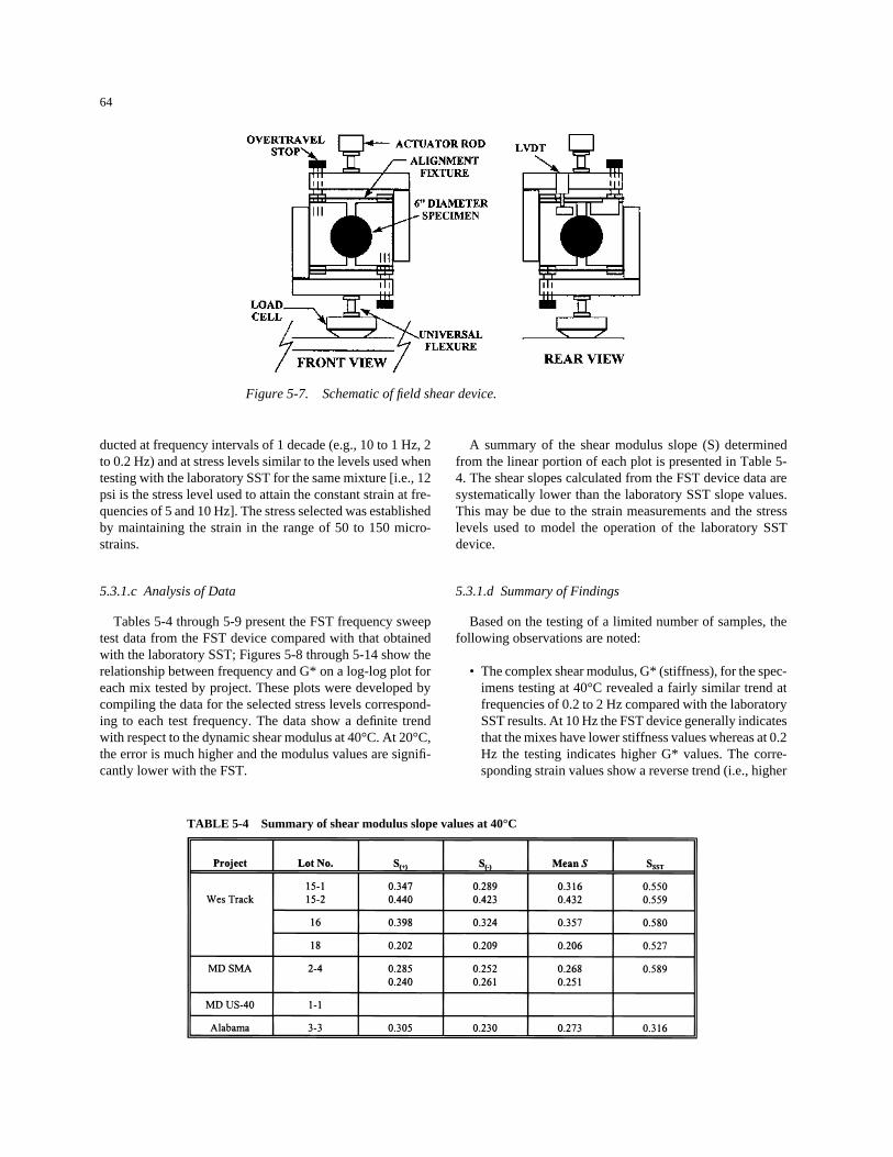
The research team reviewed relevant domestic and foreign literature on established andinnovative process control methods in the HMA industry as well as the wider manufactur-ing sector; carried out field QC/QA operations and conducted extensive laboratory testingon field- and laboratory-compacted specimens from 15 pavement projects constructed in1994, 1995, and 1996; evaluated a variety of test methods and equipment for contractor con-trol of field operations with Superpave-designed HMA; and developed a prototype fieldshear test (FST) device to measure key HMA performance properties during pavement construction.
This NCHRP report presents several products expected to facilitate the wider imple-mentation of the Superpave mix design method: a QC/QA plan, including tolerances forkey materials and volumetric mix properties, for field production and lay down of HMA
produced in accordance with Superpave material specifications and mix designs method(Chapter 2); guidelines for adjustment of production and placement of HMA to maintainconformance with Superpave specifications and mix designs (Chapter 3); a training pro-gram (available in the form of a Microsoft Powerpoint presentation) for qualifying techni-cians to use the procedures set forth in the QC/QA plan (Chapter 4); and equipment require-ments, test procedures, and data analysis techniques for use of the Superpave gyratorycompactor as the principal tool in QC/QA operations, and for the FST device and the rapidtriaxial test that with further development may complement the gyratory compactor in suchoperations (Chapter 5).
The QC/QA plan presented in Chapter 2 establishes minimum requirements and activ-ities for a contractor’s QC system related to Superpave mix design, production, placement,and compaction. These requirements include a listing of the inspections and tests necessaryto substantiate material and product conformance to the Superpave mix design. The primarymethod of field QC employs the Superpave gyratory compactor and evaluation of the vol-umetric properties of the mix.
The plan also establishes requirements for a state highway agency’s assessment andacceptance of a project incorporating Superpave-designed HMA. This plan, coupled withthe contractor’s QC plan, provides the necessary quality assurance for control, verification,and acceptance of the project.
1 CHAPTER 1 Quality Control and Acceptance of Superpave-Designed Hot MixAsphalt
1.1 Introduction, 1
3 CHAPTER 2 QC/QA Plan for Production and Lay Down of Superpave HMA2.1 Scope, 3
2.1.1 Functions and Responsibilities, 32.1.2 QC System, 3
2.6 Nonconforming Materials, 72.7 SHA Inspection at Subcontractor or Supplier Facilities, 72.8 Superpave Quality Acceptance Plan, 7
2.8.1 Scope, 82.8.2 Acceptance Plan Approach for Superpave-Designed HMA, 82.8.3 Superpave PGAB Certification, 82.8.4 Superpave Specifications and Mix Verifications, 102.8.5 Acceptance Criteria for Superpave-Designed HMA, 122.8.6 Pavement Compaction, 13
14 ANNEX I Conformal Index Approach16 ANNEX II Stratified Random Sampling Approach21 ANNEX III Statistical Control Charts
24 CHAPTER 3 Guidelines for Adjusting the Production and Placement of Superpave-Designed HMA
3.1 Noncomplying Gradation Tests, 243.1.1 Incoming Aggregates, 243.1.2 Combined Hot Bin Aggregate, 24
3.2 Noncomplying HMA Test Results, 243.2.1 Air Voids Above or Below Specifications, 243.2.2 VMA, 253.2.3 Increasing VMA, 253.2.4 Decreasing VMA, 253.2.5 VFA, 25
3.3 Noncomplying Field Density Tests, 253.4 Miscellaneous Irregularities in Pavement, 26
3.4.1 Checking and Cracking of Newly Constructed Pavement, 263.4.2 Shoving of the Compacted Pavement, 263.4.3 Raveling in the Finished Pavement, 263.4.4 Tender Pavements, 26
27 CHAPTER 4 A Training Course to Implement QC/QA Plans for Productionand Placement of Superpave-Designed HMA
4.1 Introduction, 274.2 Overview of Training Course, 27
58 CHAPTER 5 Equipment to Support Superpave QC/QA Plan5.1 Introduction, 585.2 Gyratory Compaction Control, 58
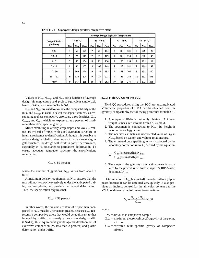
5.2.1 Volumetric Property Control, 585.2.2 Gyratory Compaction, 595.2.3 Field QC Using the SGC, 60
AUTHOR ACKNOWLEDGMENTSThe research effort reported herein was performed under
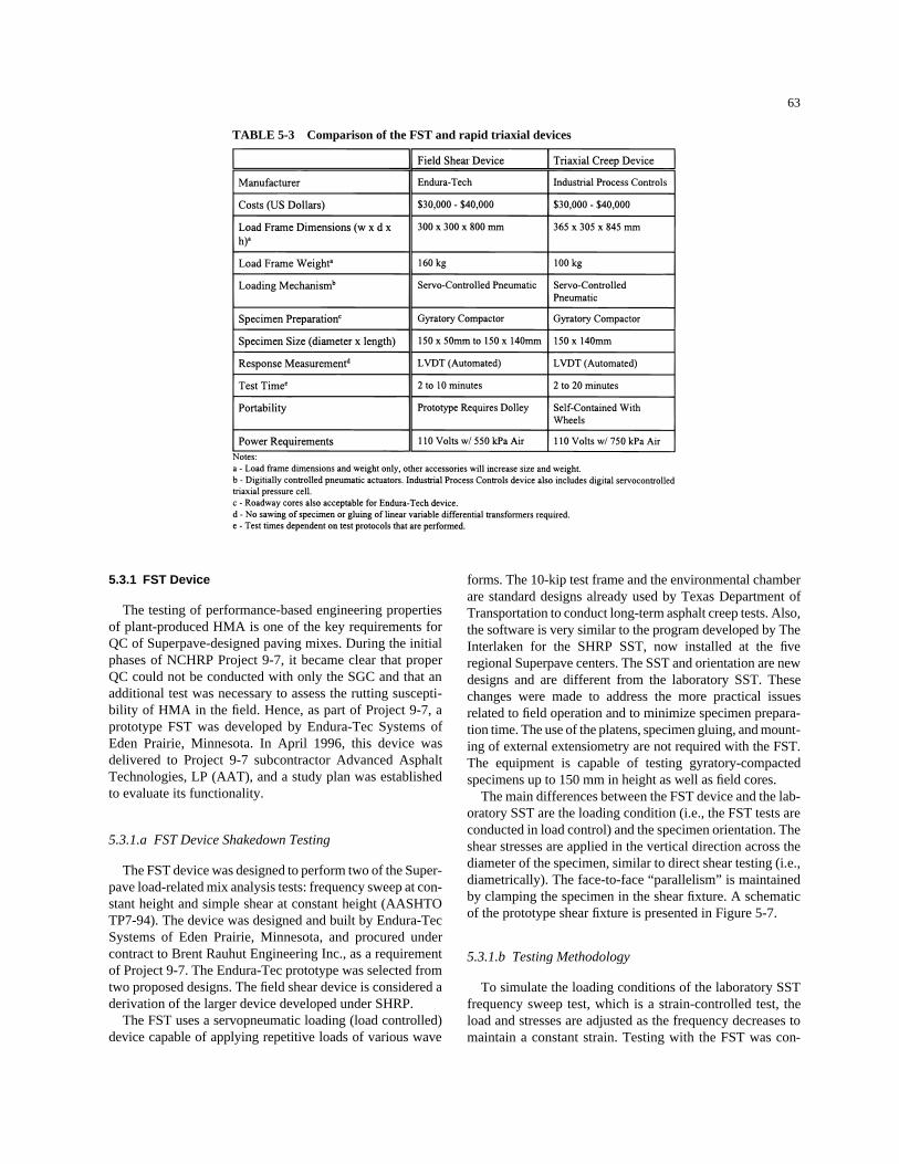
NCHRP Project 9-7 by Brent Rauhut Engineering Inc., whichserved as the prime contractor. Subcontractors for the projectincluded the Pennsylvania Transportation Institute, the AsphaltInstitute, Advanced Asphalt Technologies, the Texas Transporta-tion Institute, and Law Engineering. In addition, Industrial ProcessControls generously provided test equipment and staff involvementat no cost to the project.
Mr. Ronald J. Cominsky, formerly of BRE Inc., now ExecutiveDirector of the Pennsylvania Asphalt Pavement Association,served as the Principal Investigator for the project and primaryauthor of this report. Valuable assistance in conducting the projectand authoring the report was provided by Mr. Brian M. Killings-worth of BRE Inc. Others who contributed to this report includeDr. David A. Anderson (Pennsylvania Transportation Institute),Mr. R. Michael Anderson (Asphalt Institute), Mr. Vince Aurilio(Advanced Asphalt Technologies), Dr. Thomas W. Kennedy (Uni-versity of Texas at Austin), Dr. Robert L. Lytton (Texas Trans-
portation Institute), and Dr. Bill Crockford (formerly of the TexasTransportation Institute, now a representative of Industrial ProcessControls through TSL Services and Equipment).
The authors also acknowledge the valuable assistance of Ms. TerhiPellinen (formerly of Advanced Asphalt Technologies, now withthe University of Maryland) for her efforts. Three consultants alsoprovided valuable assistance: Dr. Matthew Witczak, Mr. GarlandSteele, and Mr. James Scherocman. Mr. Barry Tritt (IndustrialProcess Controls) is also acknowledged for providing valuableinformation and test data to the project from test equipment devel-oped by IPC.
The authors also acknowledge the cooperation of several StateHighway Agencies and contractors who participated in the produc-tion and construction of field test sites. The States that participatedinclude Kentucky, Virginia, Florida, Texas, Mississippi, Alabama,Georgia, Kansas, Maryland, and Louisiana. Material was also sam-pled and tested from test sections constructed at WesTrack inNevada.
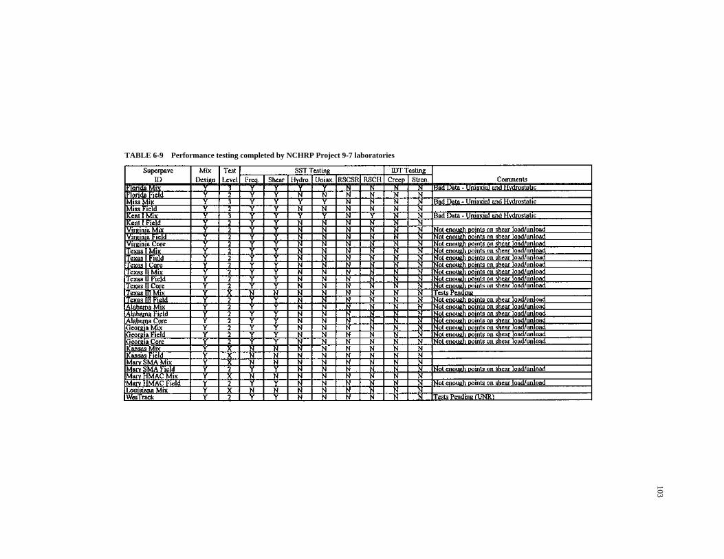
77 CHAPTER 6 Summary of the Research Project6.1 Introduction, 776.2 Objectives and Organization of the Research, 776.3 Conduct of the Research, 78
6.3.1 Phase I: Literature Surveys, 786.3.2 Phase II: Experiment Design and Field Experiments, 90
110 APPENDIX A Additional Training Modules
110 APPENDIX B Field Shear Test Procedure in AASHTO Draft Fomat
110 APPENDIX C Rapid Triaxial Test Procedure in AASHTO Draft Format
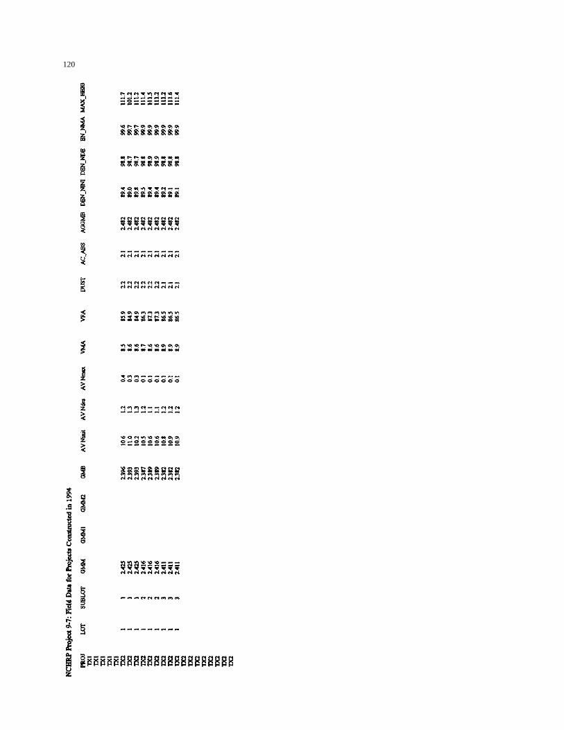
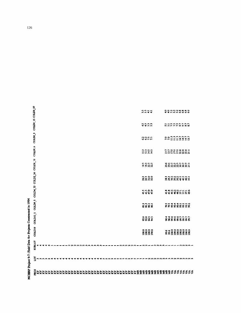
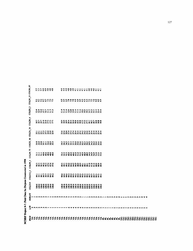
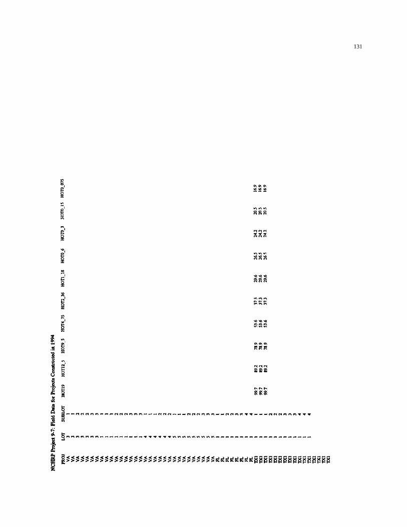
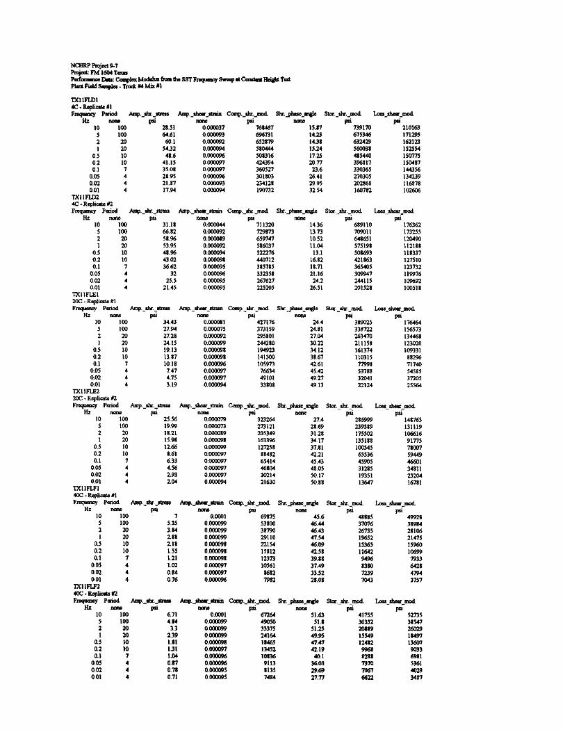
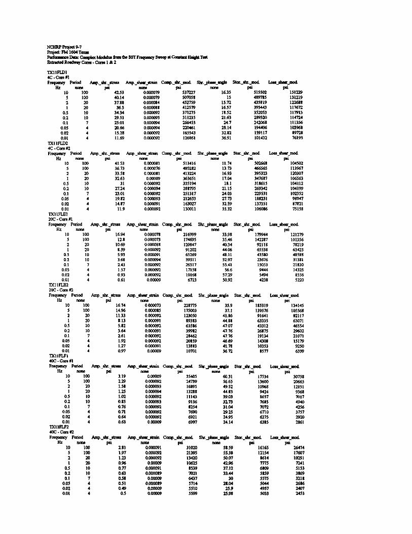
111 APPENDIX D Summary of Information for Projects Constructed in 1994
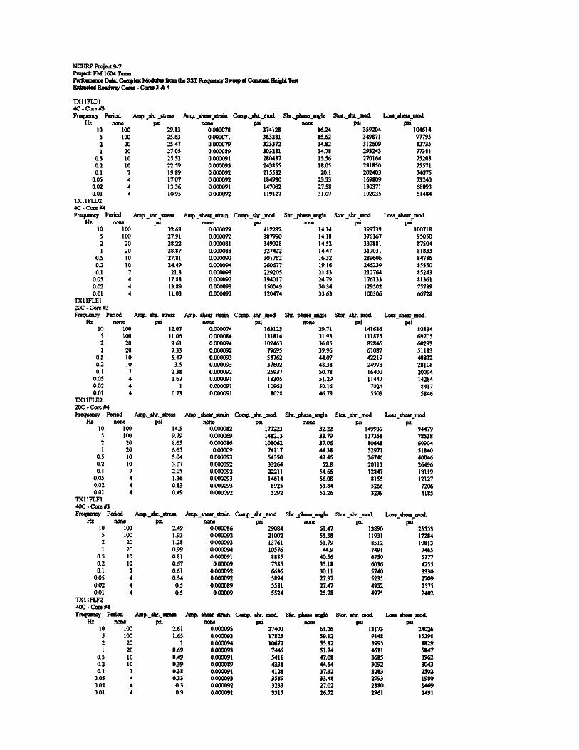
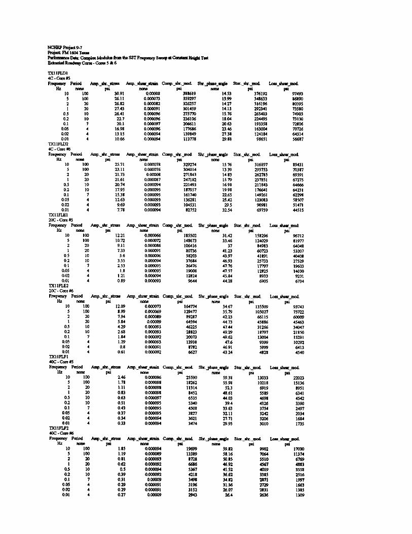
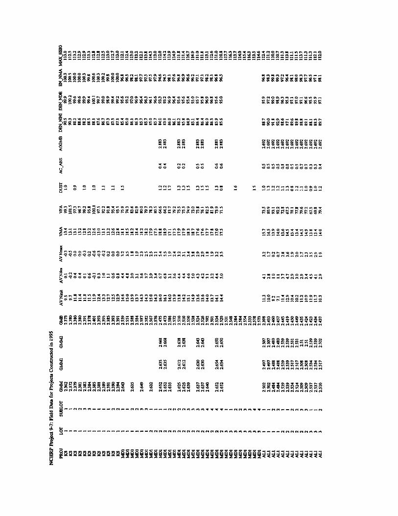
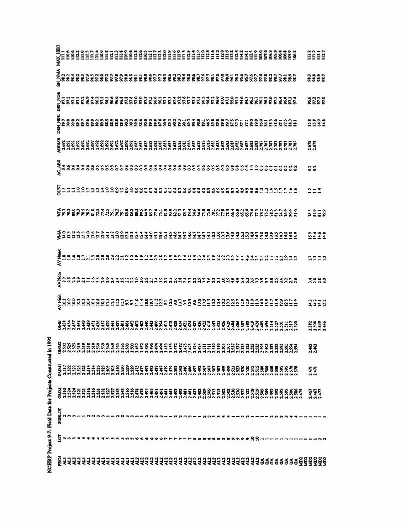
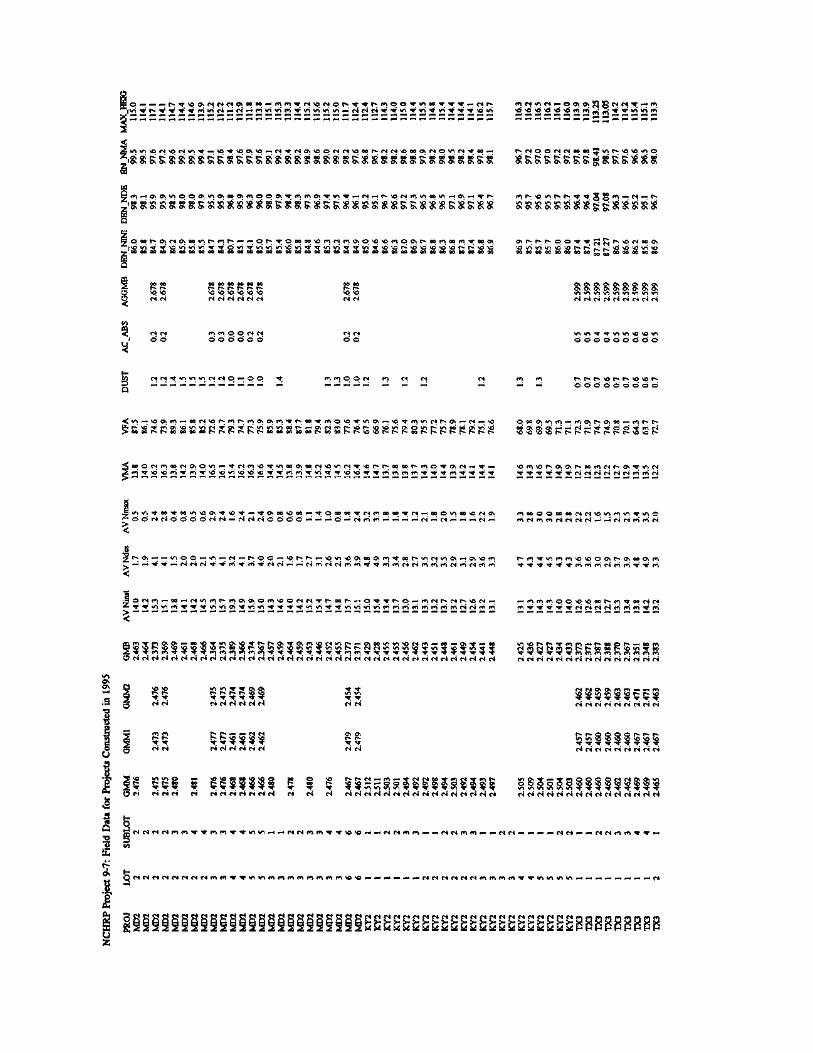
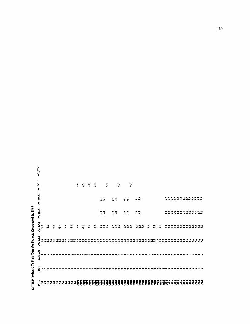
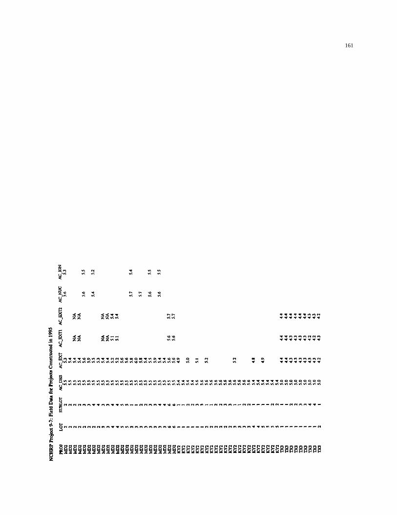
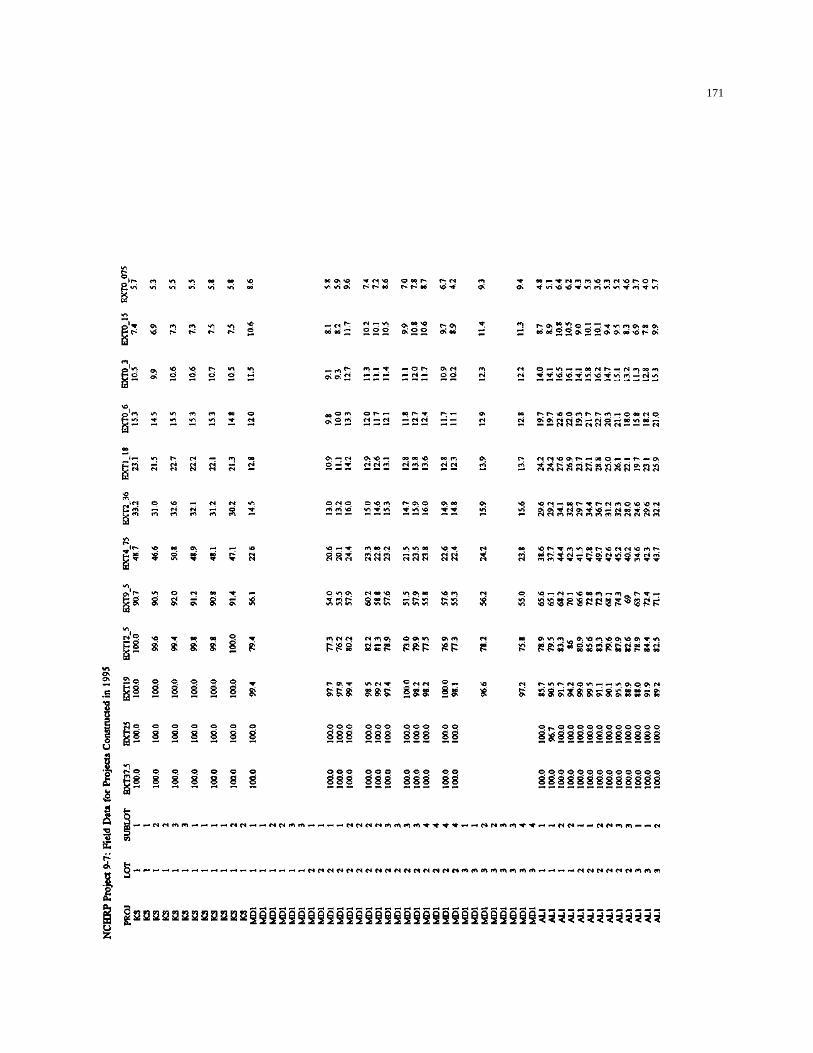
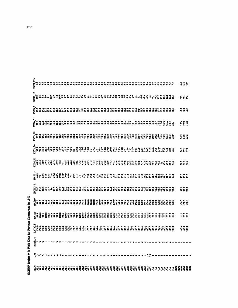
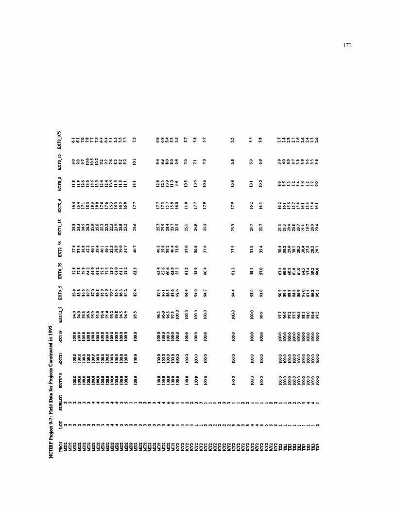
149 APPENDIX E Summary of Information for Projects Constructed in 1995
177 APPENDIX F Summary of Information for Verification of Version 2.0 QC/QAPlan
178 APPENDIX G Comparison of Quality Control and Acceptance Tests
184 APPENDIX H Quality Control Testing of Asphalt Binders
185 APPENDIX I Sensitivity of SUPERPAVE Mixture Tests to Changes in Mixture Components
1
CHAPTER 1
QUALITY CONTROL AND ACCEPTANCE OF SUPERPAVE-DESIGNED HOT MIX ASPHALT
1.1 INTRODUCTION
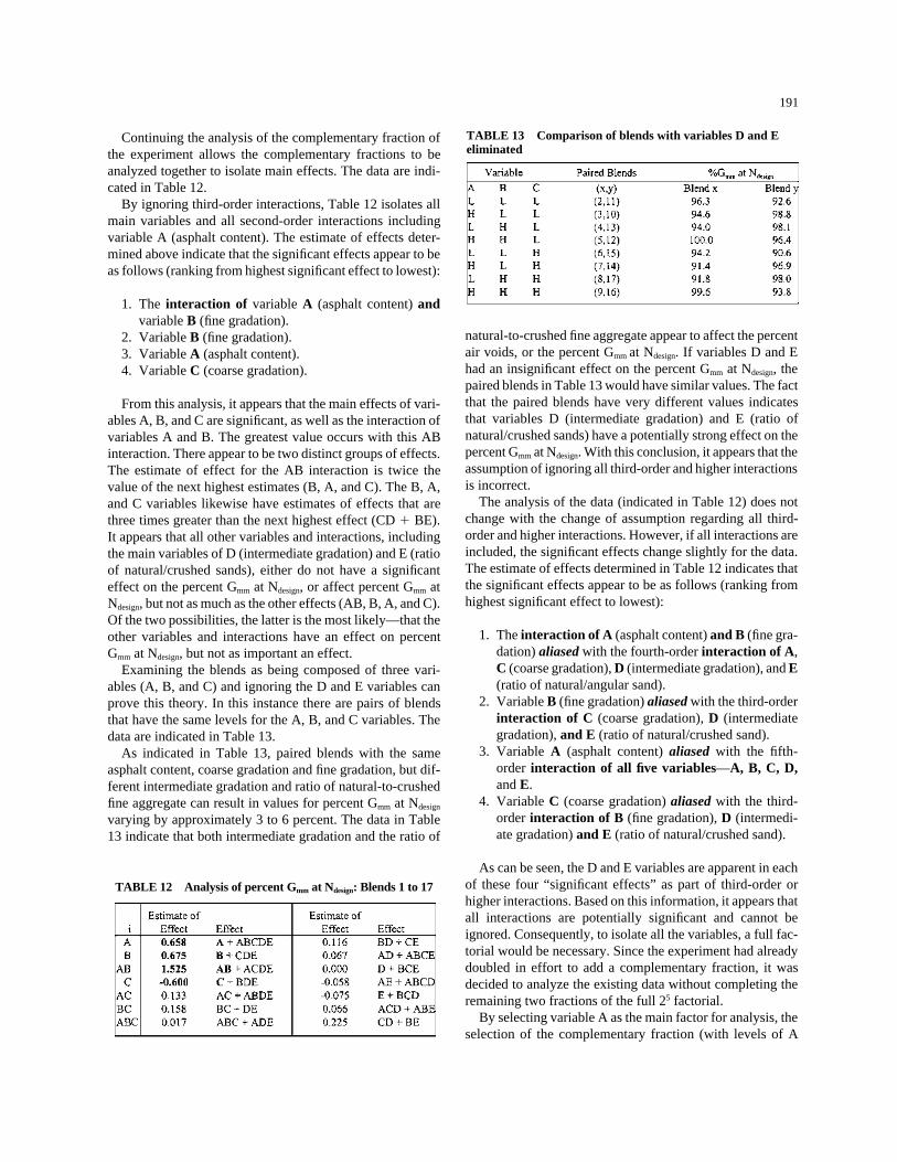
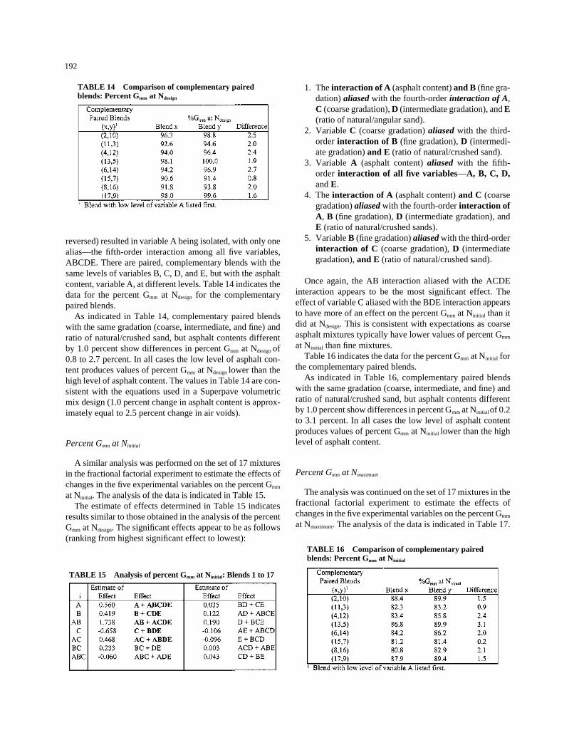
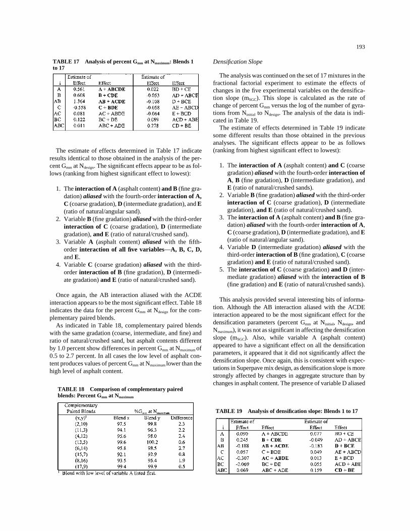
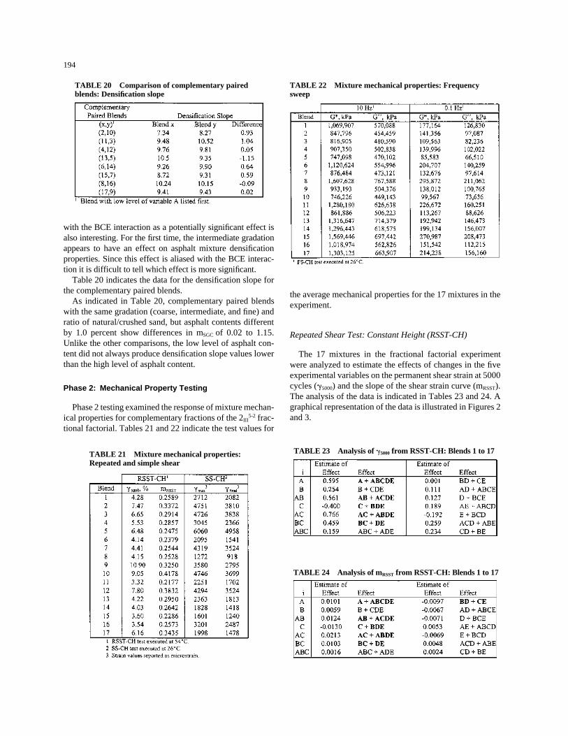
Interest in the Superpave performance-based mix designand analysis system, developed through the asphalt researchprogram of the Strategic Highway Research Program (SHRP),is rapidly growing throughout the nation. AASHTO memberdepartments are actively gearing up for Superpave imple-mentation. The AASHTO Task Force on SHRP Implementa-tion has targeted SHRP’s asphalt products as one of its pri-orities. Members of the AASHTO Highway Subcommitteeon Materials are evaluating more than 20 specific products inthe asphalt area. A pooled-fund study has assisted the statesto obtain the necessary laboratory test equipment. The Fed-eral Highway Administration (FHWA) has established fiveSuperpave Regional Centers nationally to assist state highwayagencies (SHAs) with Superpave implementation. Industrymust be involved, however, to fully implement SHRP’s rec-ommendations and will need the knowledge and tools to com-ply with the new requirements. To that end, user-producergroups are operating on a regional basis, involving SHAs,contractors, and materials manufacturers and suppliers. Infor-mation presented to these groups, initially by SHRP and nowby the FHWA, has built wide-ranging support for adoption ofthis new system of material specifications, test methods andequipment, design and analysis practices, and software.
Such significant improvements in asphalt binders, testequipment and procedures, analysis of test results, and spec-ifications should provide a substantially greater level of per-formance from paving mixes designed with the Superpavesystem. However, to realize these improvements, SHAs mustensure that the production, placement, and compaction ofpaving mixes in field projects are controlled to maintain com-pliance with the specifications.
A general approach to field control procedures was devel-oped under SHRP to assist field technicians in adjusting mixdesign and monitoring production. The need was identifiedfor additional research to specifically provide SHAs andpaving contractors with appropriate quality control and qual-ity assurance (QC/QA) procedures for the field implementa-tion of the Superpave material specifications and mixdesigns. NCHRP Project 9-7, “Field Procedures and Equip-ment to Implement SHRP Asphalt Specifications,” was initi-ated to satisfy this requirement.
NCHRP Project 9-7 had two key objectives:
• To establish comprehensive procedures and, if required,develop equipment for QC/QA at the asphalt plant and laydown site to ensure that hot mix asphalt (HMA) meets theSuperpave performance-based specifications and
• To develop a framework for a training program for qual-ifying technicians to accomplish these QC/QA proce-dures.
After a review of the SHRP asphalt research program resultsand discussion with the NCHRP Project 9-7 panel, a decisionwas made to consider only permanent deformation as a dis-tress factor. Permanent deformation is a short-term phenome-non that can be evaluated by QC/QA field testing. Pavementfatigue is a long-term phenomenon that is generally addressedthrough pavement layer thickness determination during thepavement design process. Low-temperature cracking is ad-dressed during the Superpave mix design process by the selec-tion of the appropriate performance grade of asphalt binder.
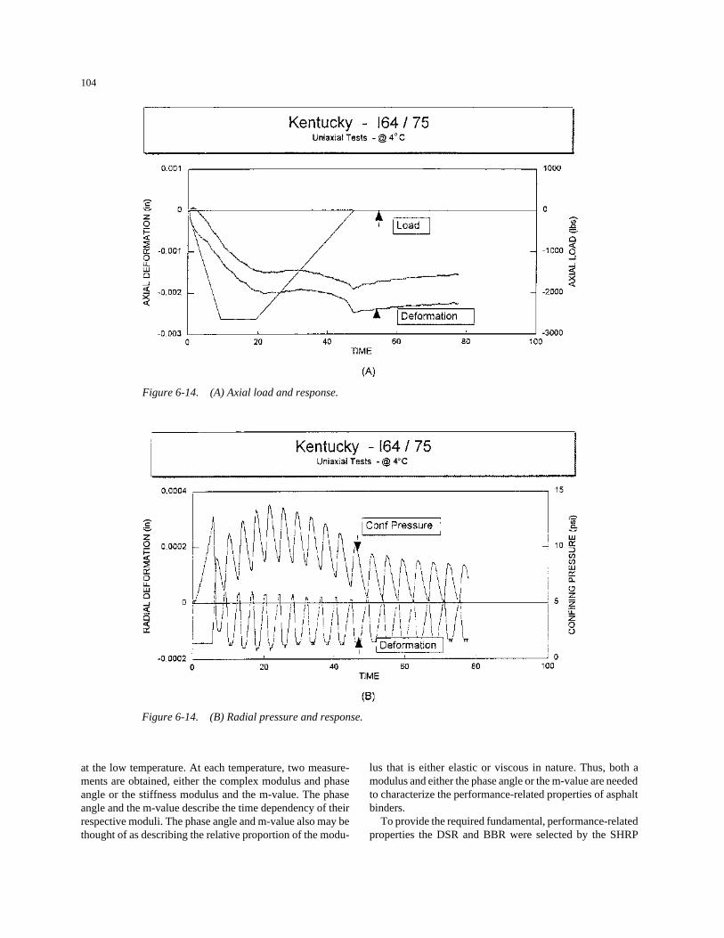
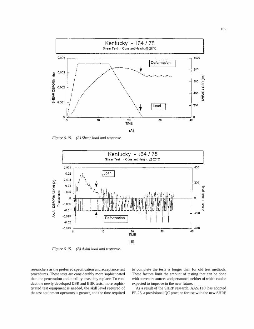
This report presents QC/QA procedures developed on thebasis of experimental data obtained from 14 field paving proj-ects during the course of the project. The report assumes afamiliarity with the Superpave mix design procedures includ-ing the use of the Superpave gyratory compactor (SGC).1
Although the current focus of the SHAs is on the Super-pave volumetric mix design method (originally termedSuperpave level 1), Project 9-7 also considered the originalSuperpave level-2 and Superpave level-3 design procedures(now termed abbreviated and full mix analyses) recom-mended by SHRP. Further, in this report the QC function isassigned specifically to the paving Contractor and the QAfunction is assigned solely to the SHA.
The report is organized in two parts. Part I (Chapters 2through 6) provides specific details of the products deliveredby the research project and is intended for the practitionerand the user. Part I includes the following:
• A QC/QA plan for field production and lay down ofHMA produced in accordance with Superpave materialspecifications and mix design method (Chapter 2);
1AASHTO TP4, Standard Method for Preparing and Determining the Density ofHMA Specimens by Means of the SHRP Gyratory Compactor.
• Guidelines for adjustment of production and placementof Superpave-designed HMA (Chapter 3);
• A training program for qualifying technicians to use theprocedures set forth in the QC/QA plan (Chapter 4);
• A description of two field-testing devices that supportthe SGC for QC practices and provisional test proce-dures and data analysis for their use (Chapter 5); and
• A summary of the research results of NCHRP Project 9-7 and the conclusions drawn from the results that formthe basis for the QC/QA practices and suggested guide-lines for mix and placement adjustments (Chapter 6).
The appendices form Part II of the report. They providecomplete experimental details and results upon which theproducts presented in Chapters 2 through 5 are based. Theappendices include the following:
• Additional training information that can be used forassisting in the implementation of Superpave activities(Appendix A);
2
• Test procedures for the field QC devices developed dur-ing the project (Appendices B and C);
• The Stage I research approach: Superpave mix designs forsix experimental construction projects conducted in 1994;QC data for the six projects; statistical analyses; and con-clusions for the Version 1 QC/QA plan (Appendix D);
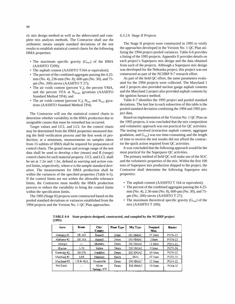
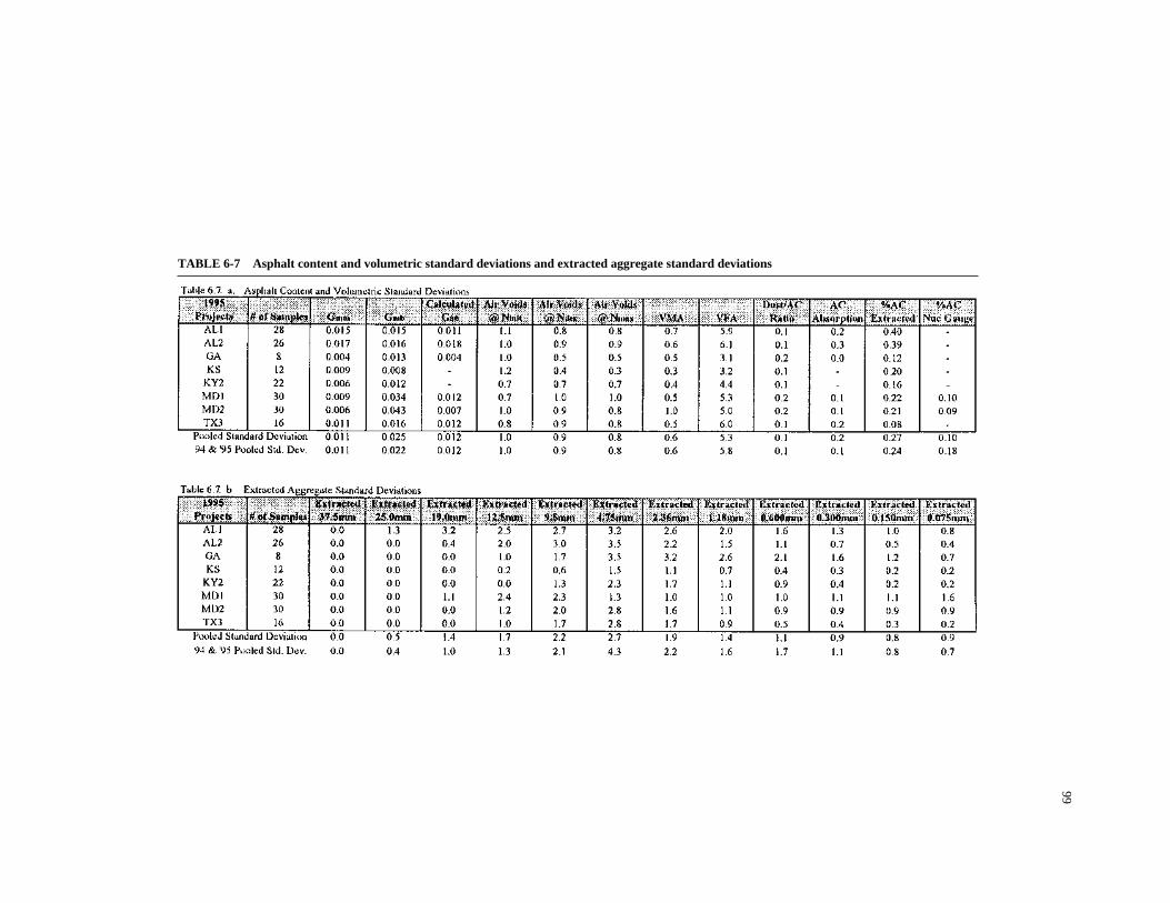
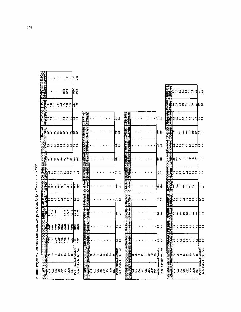
• The Stage II research approach: Superpave mix designsfor seven experimental construction projects in 1995; QCdata for the seven projects; statistical analyses; and con-clusions for the Version 2 QC/QA plan (Appendix E);
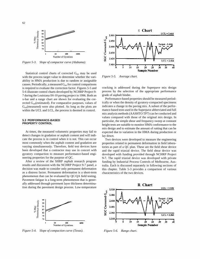
• Verification of the Version 2.0 QC/QA plan; Superpavemix design for a project in Louisiana on which the Ver-sion 2.0 plan was used; statistical control charts; com-paction data, and statistical analyses (Appendix F);
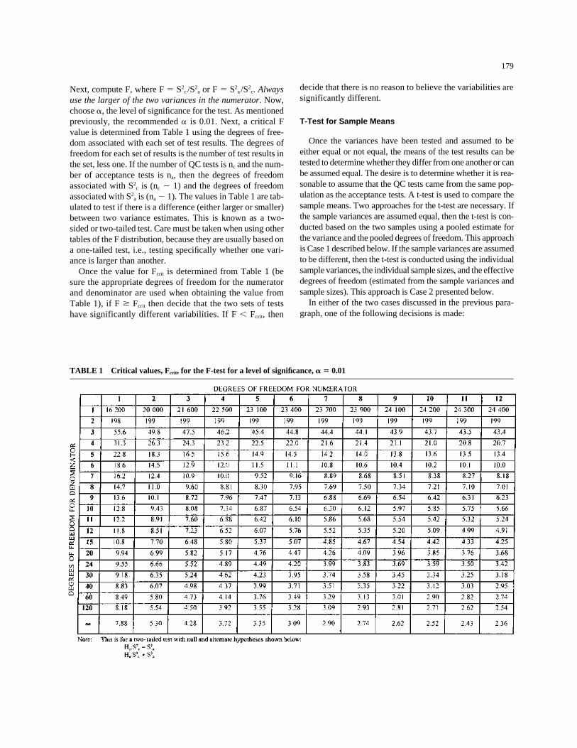
• Dispute resolution: Statistically based guidelines forcomparison of QC and QA data adopted by AASHTO(Appendix G);
QC/QA PLAN FOR PRODUCTION AND LAY DOWN OF SUPERPAVE HMA
This chapter presents the specific details necessary toeffectively control the production and lay down of Superpavemixes. The need for and use of a QC function cannot beoveremphasized for the Superpave mix. Quality cannot betested or inspected into the Superpave mix; it must be “builtin.” As discussed in the AASHTO QC/QA Specification andImplementation Guide, QC should be completed by the Con-tractor. Thus, it is imperative that the Contractor have a func-tional, responsive QC Plan. When a Contractor’s QC Plan isinitially required, minimum requirements are helpful as aguide to the Contractor. This approach provides a uniformbasis for bidding and ensures a minimum level of QC. It isimportant that a QC Plan address the actions needed, includ-ing the frequency of testing to (a) keep the process in control,(b) quickly determine when it goes out of control, and (c)respond adequately to bring the process back into control.
2.1 SCOPE
This QC Plan establishes minimum requirements andactivities for a Contractor’s QC system related to the Super-pave mix design. These requirements pertain to the inspec-tions and tests necessary to substantiate material and productconformance to the Superpave mix design requirements andto all related inspections and tests. The primary method offield QC employs the use of the SGC and evaluation of thevolumetric properties of the mix.
This QC Plan shall apply to all construction projects usinga Superpave mix design when so indicated in the contractdocuments. If there are inconsistencies between the contractdocuments and this QC Plan, the contract documents shallcontrol.
2.1.1 Functions and Responsibilities
2.1.1.a SHA
The SHA will verify the Superpave volumetric mixdesigns, inspect plants, and monitor control of the operationsto ensure conformity with the Superpave mix requirements.
At no time will the SHA representative issue instructionsto the Contractor or Producer about setting dials, gauges,scales, and meters. However, the SHA representatives will
have the responsibility to question and warn the Contractoragainst the continuance of any operations or sequence ofoperations that will obviously not result in satisfactory com-pliance with Superpave mix requirements.
2.1.1.b The Contractor
The Contractor shall be responsible for development andformulation of the Superpave mix design, which will be sub-mitted to the SHA for verification. In addition, the Contrac-tor shall be responsible for the process control of all materi-als during the handling, blending, mixing, and placingoperations.
2.1.2 QC System
2.1.2.a General Requirements
The Contractor shall provide and maintain a QC systemthat will provide reasonable assurance that all materials andproducts submitted to the SHA for acceptance conform to theSuperpave specification requirements whether manufacturedor processed by the Contractor or procured from suppliers orsubcontractors. The Contractor shall perform or have per-formed the inspection and tests required to substantiate prod-uct conformance to the Superpave volumetric mix designrequirements and shall also perform or have performed allinspections and tests otherwise required by the SHA contract.The Contractor’s QC procedures, inspections, and tests shallbe documented and shall be available for review by the SHAfor the life of the contract.
2.1.2.b Documentation
The Contractor shall maintain adequate records of allinspections and tests. The records shall indicate the natureand number of observations made, the number and type ofdeficiencies found, the quantities approved and rejected, andthe nature of corrective action taken as appropriate. The Con-tractor’s documentation procedures will be subject to thereview and approval of the SHA before the start of the workand the compliance checks during the progress of the work.
All charts and records documenting the Contractor’s QCinspections and tests shall become property of the SHA uponcompletion of the work.
2.1.2.c Charts and Forms
All conforming and nonconforming inspections and testresults shall be recorded on appropriate forms and charts,which shall be kept up to date and complete and shall be avail-able at all times to the SHA during performance of the work.Test properties for the various materials and mixtures shall becharted on forms or other appropriate means, which are inaccordance with the applicable requirements of the SHA.
2.1.2.d Corrective Action
The Contractor shall take prompt action to correct condi-tions that have resulted or could result in the submission ofmaterials, products, and completed instructions that do notconform to the requirements of the SHA Superpave specifi-cation requirements.
2.1.2.e Measuring and Testing Equipment
The Contractor shall provide and maintain measuring andtesting apparatus necessary to ensure that the materials andproducts conform to the Superpave specification require-ments. To ensure continued accuracy, the apparatus shall beinspected and calibrated at established intervals against rele-vant SHA standards. In addition, the Contractor’s personnelshall be appropriately qualified through specified accredita-tion procedures for obtaining and processing samples and foroperating such apparatus and for verifying their accuracy andcondition. Calibration results shall be available to the SHAat all times.
The QC of the Superpave PGAB will be in accordancewith AASHTO PP26-96, “Standard Practice For CertifyingSuppliers of Performance-Graded Asphalt Binders.”
2.2.2 AASHTO PP26-96 Standard
AASHTO PP26-96 specifies requirements and proceduresfor a certification system that shall be applicable to all sup-pliers of PGAB. The requirements and procedures shall applyto materials that meet the requirements of AASHTO stan-dard MP1 “Specifications for Performance-Graded AsphaltBinders,” Section 5, Materials and Manufacture, and that are
4
manufactured at refineries, mixed at terminals, in-lineblended, or modified at the HMA plant. Sections 9 and 13 ofthe AASHTO PP26-96 are of primary importance to theHMA plant operations related to PGAB certification and QC.
2.3 SUPERPAVE MIX DESIGN AND PRODUCTION
2.3.1 Laboratory Trial Mix Formula (LTMF) and HMA Plant Laboratory Verification
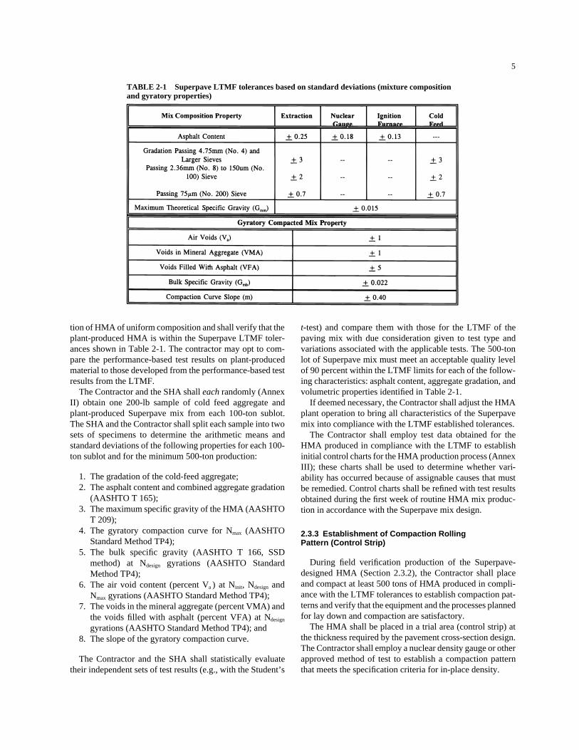
The Contractor shall develop a Superpave LTMF for theHMA paving courses by the Superpave mix design proce-dure employing the volumetric mix design concept with thegyratory compactor. The Contractor will perform a mixanalysis using the Superpave performance tests whendeemed necessary by the SHA Superpave specifications.
At least 1 month before the start of construction (or whenthe construction materials are available), the Contractor shallverify in the laboratory that the paving mixes prepared fromthe asphalt binder, coarse and fine aggregate, and mineralfiller, when necessary, planned for use in the pavement con-struction yield mix composition and gyratory-compacted(AASHTO Standard Method TP4) properties within theLTMF tolerances listed in Table 2-1. The Contractor shall beresponsible for setting the HMA plant to produce the hot mixwithin the LTMF tolerances (standard deviation ) specified inTable 2-1 for the mix composition and gyratory-compactedmix properties. Annex I provides an alternative approachusing conformal indices in lieu of standard deviations. Thevalues in Table 2-1 were developed for individual samples (n � 1). For larger sample sizes, the standard deviation val-ues in Table 2-1 must be adjusted by the following equation:
where�x– � standard deviation of sample means of sample size n� � standard deviation from Table 2-1n � sample size
The Contractor shall report to the SHA, in writing, theresults of this laboratory verification and any actions neces-sary in the Contractor’s judgment to bring the paving mixesproduced with the materials planned for use in the pavementconstruction into conformance with the LTMF Superpavetolerances. The Contractor shall not proceed to the field ver-ification (Section 2.3.2) without the approval of the SHA.
2.3.2 Field Verification and Adjustment to the LTMF
At the beginning of the project, the contractor shall pro-duce a minimum of 500 tons but not exceed a day’s produc-
σ σx n
=
tion of HMA of uniform composition and shall verify that theplant-produced HMA is within the Superpave LTMF toler-ances shown in Table 2-1. The contractor may opt to com-pare the performance-based test results on plant-producedmaterial to those developed from the performance-based testresults from the LTMF.
The Contractor and the SHA shall each randomly (AnnexII) obtain one 200-lb sample of cold feed aggregate andplant-produced Superpave mix from each 100-ton sublot.The SHA and the Contractor shall split each sample into twosets of specimens to determine the arithmetic means andstandard deviations of the following properties for each 100-ton sublot and for the minimum 500-ton production:
1. The gradation of the cold-feed aggregate;2. The asphalt content and combined aggregate gradation
(AASHTO T 165);3. The maximum specific gravity of the HMA (AASHTO
T 209);4. The gyratory compaction curve for Nmax (AASHTO
Standard Method TP4);5. The bulk specific gravity (AASHTO T 166, SSD
method) at Ndesign gyrations (AASHTO StandardMethod TP4);
6. The air void content (percent Va ) at Ninit, Ndesign andNmax gyrations (AASHTO Standard Method TP4);
7. The voids in the mineral aggregate (percent VMA) andthe voids filled with asphalt (percent VFA) at Ndesign
gyrations (AASHTO Standard Method TP4); and8. The slope of the gyratory compaction curve.
The Contractor and the SHA shall statistically evaluatetheir independent sets of test results (e.g., with the Student’s
5
t-test) and compare them with those for the LTMF of thepaving mix with due consideration given to test type andvariations associated with the applicable tests. The 500-tonlot of Superpave mix must meet an acceptable quality levelof 90 percent within the LTMF limits for each of the follow-ing characteristics: asphalt content, aggregate gradation, andvolumetric properties identified in Table 2-1.
If deemed necessary, the Contractor shall adjust the HMAplant operation to bring all characteristics of the Superpavemix into compliance with the LTMF established tolerances.
The Contractor shall employ test data obtained for theHMA produced in compliance with the LTMF to establishinitial control charts for the HMA production process (AnnexIII); these charts shall be used to determine whether vari-ability has occurred because of assignable causes that mustbe remedied. Control charts shall be refined with test resultsobtained during the first week of routine HMA mix produc-tion in accordance with the Superpave mix design.
2.3.3 Establishment of Compaction RollingPattern (Control Strip)
During field verification production of the Superpave-designed HMA (Section 2.3.2), the Contractor shall placeand compact at least 500 tons of HMA produced in compli-ance with the LTMF tolerances to establish compaction pat-terns and verify that the equipment and the processes plannedfor lay down and compaction are satisfactory.
The HMA shall be placed in a trial area (control strip) atthe thickness required by the pavement cross-section design.The Contractor shall employ a nuclear density gauge or otherapproved method of test to establish a compaction patternthat meets the specification criteria for in-place density.
TABLE 2-1 Superpave LTMF tolerances based on standard deviations (mixture compositionand gyratory properties)
2.4 SAMPLING AND TESTING
The QC Plan recognizes that the LTMF generally is notrepresentative of the HMA that is produced in the field. Thetarget values developed from the field verification of theplant-produced HMA and the control strip will become thecontrol values. The target levels for key mix properties willbe established through the field verification of HMA produc-tion (Section 2.3.2) and the lay down of the control strip(Section 2.3.3). These include the maximum theoretical bulkspecific gravity, gyratory compaction parameters that willsubsequently be used as QC indicators, volumetric propertiessuch as percent air voids, percent VMA, percent VFA, and,if opted for by the Contractor, the performance properties.
The QC Plan is based on a concept of continuous sam-pling of Superpave HMA at the plant. Lots and sublots areconsidered in the QC Plan only for in-place compaction. TheQC sampling will progress continuously as long as the targetvalues are within the LTMF tolerances and do not changesubstantially as monitored by the control chart values. Theobjective of sampling and testing associated with this QCPlan is to ensure conformance of the mean properties of the“plant-produced” mix with the “target” mix and to minimizevariability in the HMA.
The Contractor’s QC Plan shall be based on random sam-pling and testing of the HMA at its point of production todetermine compliance with the LTMF tolerances. The Con-tractor shall measure by means approved by the SHA andrecord a daily summary including the following:
• Quantities of asphalt binder, aggregate, mineral filler,and (if required) fibers used;
• Quantities of HMA produced; and• HMA production and compaction temperatures.
The QC Plan shall include a statistically sound, random-ized sampling plan to provide samples representative of theentire HMA production and to ensure that all sampling isconducted under controlled conditions.
2.5 QC ACTIVITIES
2.5.1 Plant-Produced Superpave Mix QC
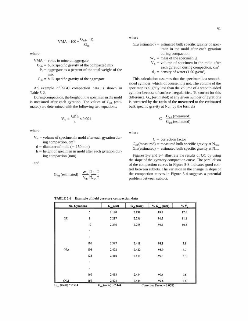
The primary method of field QC makes use of the SGCand the volumetric properties of the HMA. If the results oftesting are within LTMF tolerances of Section 2.3.2 (fieldverification and adjustments to the LTMF), the production isconsidered in control. Subsequent sampling and testing willbe performed with the estimated bulk specific gravities (Gmb
est.) at design number of gyrations (Ndes) obtained from thegyratory compactor by the following:
1. A sample is randomly obtained. A known weight ismeasured into the heated mold.
6
2. The specimen is compacted to Nmaximum. Heights arerecorded at each gyration.
3. The operator performs a calculation to determine theestimated Gmb at Ndesign.
4. The estimated bulk specific gravity is corrected by thelaboratory correction ratio
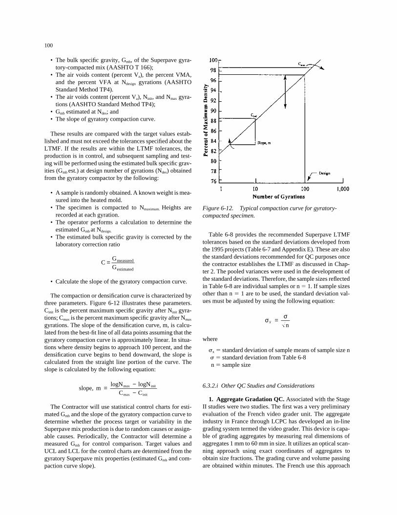
5. The slope of the gyratory compaction curve is calcu-lated by the method used in report SHRP-A-407, Sec-tion 3.7.4.1, as follows: The compaction or densifica-tion curve is characterized by three parameters. Cinit isthe percent of maximum theoretical specific gravityafter Ninit gyrations; Cmax is the percent of maximumtheoretical specific gravity after Nmax gyrations. Theslope of the densification curve, m, is calculated fromthe best-fit line of all data points assuming that thegyratory compaction curve is approximately linear. Insituations where density begins to approach 100 per-cent, and the densification curve begins to bend down-ward, the slope is calculated from the straight line por-tion of the curve. The slope is calculated by thefollowing equation:
The Contractor shall use statistical control charts for thecorrected, estimated Gmb and the slope of the gyratory com-paction curve to determine whether the process target or vari-ability in the HMA production is due to random or assign-able causes. Periodically, the Contractor will determine ameasured Gmb to validate the correction factor for controlcomparison.
Target values and upper and lower control limits for thecontrol charts are determined from the gyratory mix proper-ties (estimated Gmb and compaction curve slope) measuredduring the field verification process (Section 2.3.2) and thefirst few days of production. The grand mean and averagerange of the test data shall be used to develop x-bar (mean)and R (range) control charts for each material property. Upperand lower control limits shall be set at �2s and �3s, definedas warning and action control limits, respectively where s isthe sample standard deviation. These initial measurementsfor routine HMA production shall agree with those of the ver-ification samples tested in accordance with the requirementsof Section 2.3.2. If the control limits are not within the allow-able LTMF tolerance limits, the Contractor shall modify theHMA production process to reduce the variability and bringthe control limits within the specification limits.
Eight consecutive plotted points on either side of the tar-get value or one point outside the warning or action limitindicates a mix composition change. At this point, another
slope, mlogN logN
C Cinit
max init
= −−
max
CG measured
G estimatedmb
mb
= ( )
( )
Gmb measurement must be conducted to confirm compliancewith the target. If the results indicate noncompliance, adjust-ments must be made to the asphalt content or aggregate gra-dation to provide mixture compliance. Once adjustmentshave been made, Gmm, Gmb, asphalt content, gradation, airvoids, VMA, and VFA determinations must be made andcompared with the LTMF allowable tolerances. The Con-tractor may opt to conduct the field shear test to evaluateengineering properties.
2.5.2 QC of In-Place Compaction
The Contractor shall develop and implement a planapproved by the SHA to control the compaction of the HMAand ensure its compliance with the project specification.
The QC Plan for compaction shall include a statisticallysound, randomized sampling and testing plan using proce-dures to provide measurements of the in-place air voids con-tents representative of the entire pavement course and toensure that all sampling or testing is conducted under con-trolled conditions. Methods for sampling or testing the in-place pavement shall be approved in advance by the SHA.For purposes of QC, a lot shall be defined as a pavement sec-tion 5,000 ft long and 12 ft wide; for sampling purposes, eachlot shall be divided into a minimum of five sublots.
The Contractor shall measure and record a daily summaryof the following: the amount (truck loads and tons per truck)of HMA delivered to the paver; the temperature (�1°C) ofthe HMA in each truck on the surface of the load; and thetemperature (�1°C) of the mat at the approximate start of thecompaction process.
The Contractor shall establish a statistical control chart forthe in-place air voids content based on the percent of maxi-mum theoretical density. The minimum requirement is 93percent of maximum theoretical density and the maximum is98 percent. This property shall be determined through in situ,nondestructive measurement or sampling and testing of corespecimens. Four in situ, nondestructive measurements shallbe made or two pavement cores shall be taken and tested persublot at randomly selected pavement locations. The Con-tractor shall use the statistical control chart to determinewhether variability in the compaction is due to assignablecauses. Corrective action shall be taken by the Contractor,when necessary, to bring the in-place compaction processunder control.
Target values and control limits for the control chart willbe determined from compaction data measured during estab-lishment of the compaction (rolling) patterns (Section 2.3.3)and the first day’s pavement construction. The grand meanand average range of the test data shall be used to develop x-bar (mean) and R (range) control charts for compaction.Upper and lower control limits shall be set at �2s and �3s,defined as warning and action control limits, respectively,where s is the sample standard deviation. If the control lim-its are not within the allowable tolerance limits, namely,
7
93–98 percent of maximum theoretical density, the Contrac-tor shall modify the HMA lay down and compaction processto reduce the variability and bring the control limits withinthe specification limits.
The Contractor shall provide the SHA with copies of thecontrol charts. One test point outside the upper or lowerwarning control limit shall be considered an indication thatthe control of the lay down and compaction process may beunsatisfactory and shall require the Contractor to confirmthat the process parameters are within acceptable bounds.One test point outside the upper or lower action control limitor eight consecutive test points on one side of the target valueshall be judged as a lack of control in the lay down and com-paction process and shall require the Contractor to stop HMAproduction and lay down until the assignable cause for thelack of control is identified and remedied. The Contractorshall report within 24 h to the SHA (1) the assignable causefor the stop in production and (2) the action taken to remedythe assignable cause.
2.6 NONCONFORMING MATERIALS
The Contractor shall establish and maintain an effectiveand positive system for controlling nonconforming material,including procedures for its identification, isolation, and dis-position. Reclaiming or reworking nonconforming materialsshall be in accordance with procedures acceptable to theSHA. Chapter 3 provides suggested guidelines for adjustingthe components and HMA mix during the production and laydown processes.
2.7 SHA INSPECTION AT SUBCONTRACTOROR SUPPLIER FACILITIES
The SHA may inspect materials not manufactured withinthe Contractor’s facility. SHA inspection shall not constituteacceptance nor shall it in any way replace the Contractor’sinspection or otherwise relieve the Contractor of the respon-sibility to furnish an acceptable material or product. Wheninspection of the Subcontractor’s or Supplier’s product isperformed by the SHA, such inspection shall not be used bythe Contractor as evidence of effective inspection of suchSubcontractor’s or Supplier’s product.
Subcontracted or purchased materials shall be inspectedby the Contractor when received, as necessary, to ensure con-formance to contract requirements. The Contractor shall re-port to the SHA any nonconformance found on SHAsource-inspected material and shall require the supplier totake necessary corrective action.
2.8 SUPERPAVE QUALITY ACCEPTANCE PLAN
Acceptance sampling and testing of a Superpave-designedHMA is a prescribed procedure, usually involving stratified
sampling, which is applied to a series of lots of HMA. Theacceptance sampling and testing enable the SHA to decide onthe basis of a limited number of tests whether to accept agiven lot of plant mix or construction from the Contractor. Itmust be emphasized that the objective of acceptance sam-pling and testing is to determine a course of action (accept orreject). It is not an attempt to “control” quality.
2.8.1 Scope
Acceptance sampling is performed in accordance with anAcceptance Plan. The Acceptance Plan is the method of tak-ing a sample and making measurements on the sample, forthe purpose of determining the acceptability of a lot of mate-rial or construction. Briefly, in terms of acceptance sampling,the Acceptance Plan for the Superpave-designed HMAdefines the following:
1. Lot size,2. Number of samples or measurements,3. Sampling or measuring procedure,4. Point(s) of sampling or measurement,5. Method of acceptance, and6. Numerical value of specification limits.
The acceptance sampling and testing frequency is less thanthat used by the Contractor for QC purposes. Because theContractor tests more frequently to ascertain that the processvariation is within specification tolerances, the SHA needsonly to carry out additional work in accordance with thespecification Acceptance Plan to ensure the degree of theHMA with the Superpave mix design specification.
2.8.2 Acceptance Plan Approach for Superpave-Designed HMA
The Acceptance Plan consists of the evaluation of thepercent of material or construction within the specificationlimits (PWL) established for the Superpave-designed HMA.The following is the Acceptance Plan for estimating thePWL.
1. Locate n sampling positions on the lot by use of thetable of random numbers.
2. Make a measurement at each location or take a test por-tion and make the measurement on the test portion.
3. Average the lot measurements to find x–
4. Determine the standard deviation, s, of the lot mea-surements.
xx
ni
i
n
==∑
1
8
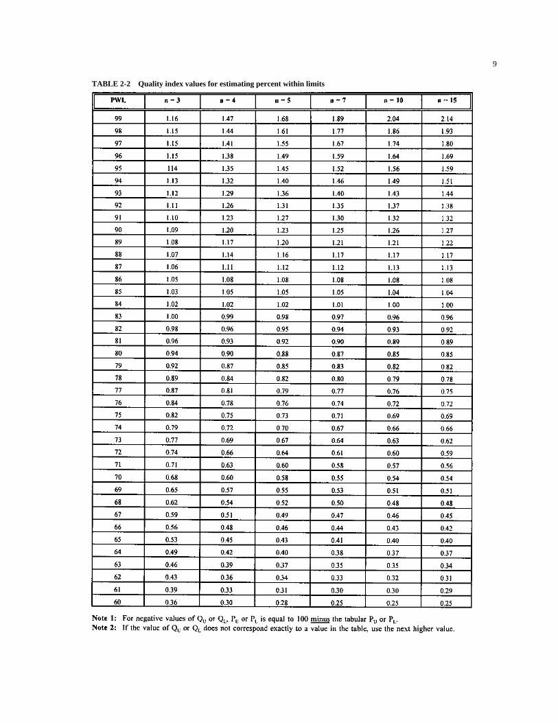
5. Find the quality index, Qu, by subtracting the average,x–, of the measurements from the upper specificationlimit, U, and dividing the results by s.
6. Find the quality index, QL , by subtracting the lowerspecification limit, L, from the average x– and dividingthe result by s.
7. Estimate the percentage of material that will fall withinthe upper tolerance limit, UTL, by entering Table 2-2,with Qu, using the column appropriate to the total num-ber, n, of measurements.
8. Estimate the percentage of material that will fall withinthe lower tolerance limit, LTL by entering Table 2-2with QL using the column appropriate to the total num-ber, n, of measurements.
9. In cases where both UTL and LTL are concerned, findthe percent of material that will fall within tolerancesby adding the percent, Pu, within the UTL to the per-cent, PL , within the LTL and subtract 100 from thesum.
2.8.3 SUPERPAVE PGAB CERTIFICATION
2.8.3.a Acceptance Criteria
The acceptance of the Superpave PGAB will be in accor-dance with AASHTO PP26-96 “Standard Practice For Cer-tifying Suppliers of Performance-Graded Asphalt Binders.”
2.8.3.b AASHTO PP26-96 Standard
AASHTO P26-96 specifies requirements and proceduresfor a certification system that shall be applicable to all sup-pliers of PGAB. The requirements and procedures shallapply to materials that meet the requirements of AASHTOStandard MP1 “Specifications for Performance-GradedAsphalt Binders,” Section 5, Materials and Manufacture, andthat are manufactured at refineries, mixed at terminals, in-line blended, or modified at the HMA plant. AASHTO P26-96. Sections 9, 10, 12, and 13 are of primary importance to
Total PWL P Pu L= + −( ) 100
Qx L
sL = −
QU x
sU = −
sx x
ni
i
n
= −−=
∑ ( )2
11
9
TABLE 2-2 Quality index values for estimating percent within limits
the SHA related to PGAB certification and acceptanceprocedures.
2.8.4 Superpave Specifications and Mix Verifications
2.8.4.a Superpave Specifications
The mix shall be designed with the Superpave mix designmethod to obtain an LTMF based on the following criteria:
10
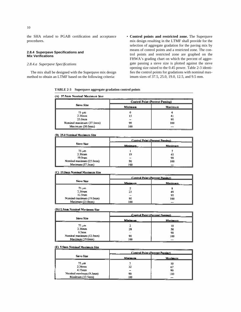
• Control points and restricted zone. The Superpavemix design resulting in the LTMF shall provide for theselection of aggregate gradation for the paving mix bymeans of control points and a restricted zone. The con-trol points and restricted zone are graphed on theFHWA’s grading chart on which the percent of aggre-gate passing a sieve size is plotted against the sieveopening size raised to the 0.45 power. Table 2-3 identi-fies the control points for gradations with nominal max-imum sizes of 37.5, 25.0, 19.0, 12.5, and 9.5 mm.
TABLE 2-3 Superpave aggregate gradation control points
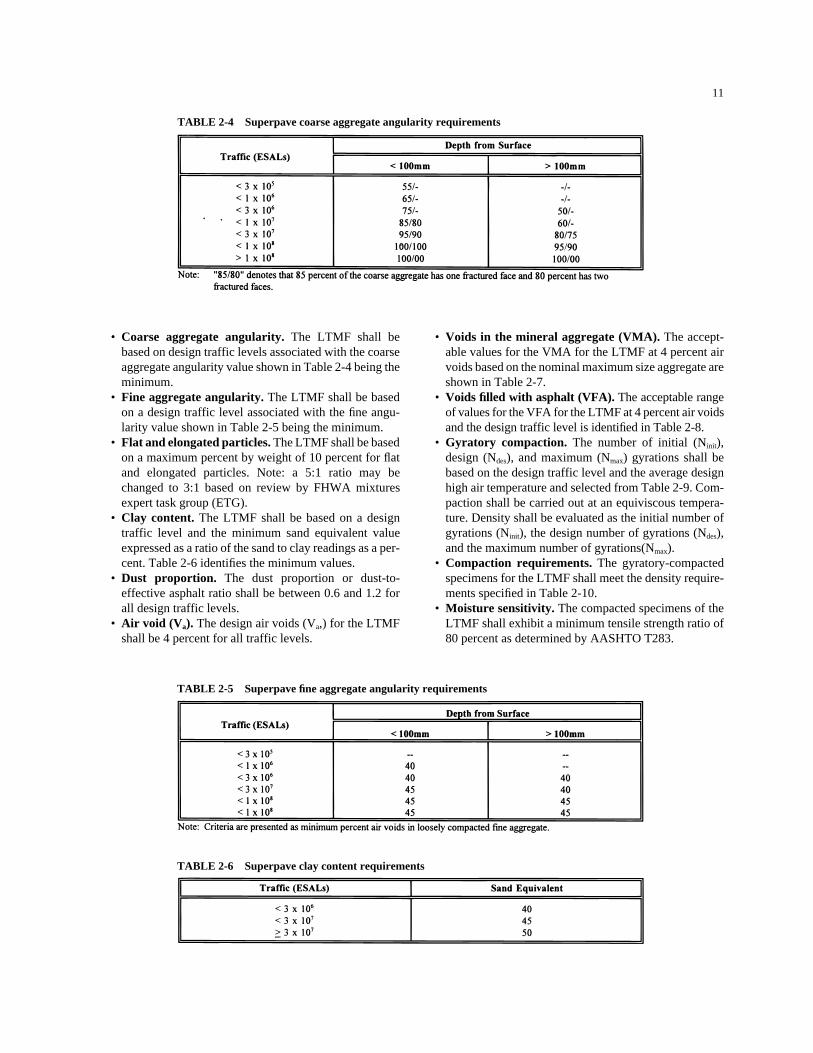
• Coarse aggregate angularity. The LTMF shall bebased on design traffic levels associated with the coarseaggregate angularity value shown in Table 2-4 being theminimum.
• Fine aggregate angularity. The LTMF shall be basedon a design traffic level associated with the fine angu-larity value shown in Table 2-5 being the minimum.
• Flat and elongated particles. The LTMF shall be basedon a maximum percent by weight of 10 percent for flatand elongated particles. Note: a 5:1 ratio may bechanged to 3:1 based on review by FHWA mixturesexpert task group (ETG).
• Clay content. The LTMF shall be based on a designtraffic level and the minimum sand equivalent valueexpressed as a ratio of the sand to clay readings as a per-cent. Table 2-6 identifies the minimum values.
• Dust proportion. The dust proportion or dust-to-effective asphalt ratio shall be between 0.6 and 1.2 forall design traffic levels.
• Air void (Va). The design air voids (Va,) for the LTMFshall be 4 percent for all traffic levels.
11
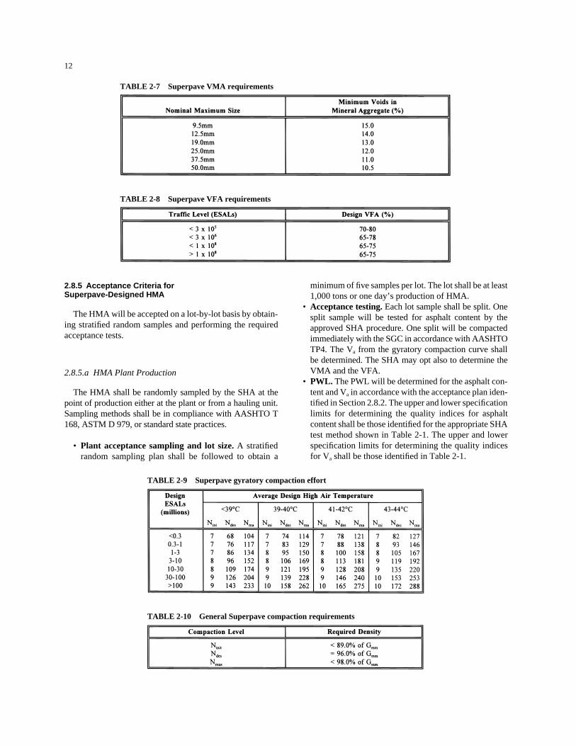
• Voids in the mineral aggregate (VMA). The accept-able values for the VMA for the LTMF at 4 percent airvoids based on the nominal maximum size aggregate areshown in Table 2-7.
• Voids filled with asphalt (VFA). The acceptable rangeof values for the VFA for the LTMF at 4 percent air voidsand the design traffic level is identified in Table 2-8.
• Gyratory compaction. The number of initial (Ninit),design (Ndes), and maximum (Nmax) gyrations shall bebased on the design traffic level and the average designhigh air temperature and selected from Table 2-9. Com-paction shall be carried out at an equiviscous tempera-ture. Density shall be evaluated as the initial number ofgyrations (Ninit), the design number of gyrations (Ndes),and the maximum number of gyrations(Nmax).
• Compaction requirements. The gyratory-compactedspecimens for the LTMF shall meet the density require-ments specified in Table 2-10.
• Moisture sensitivity. The compacted specimens of theLTMF shall exhibit a minimum tensile strength ratio of80 percent as determined by AASHTO T283.
TABLE 2-5 Superpave fine aggregate angularity requirements
TABLE 2-6 Superpave clay content requirements
2.8.5 Acceptance Criteria for Superpave-Designed HMA
The HMA will be accepted on a lot-by-lot basis by obtain-ing stratified random samples and performing the requiredacceptance tests.
2.8.5.a HMA Plant Production
The HMA shall be randomly sampled by the SHA at thepoint of production either at the plant or from a hauling unit.Sampling methods shall be in compliance with AASHTO T168, ASTM D 979, or standard state practices.
• Plant acceptance sampling and lot size. A stratifiedrandom sampling plan shall be followed to obtain a
12
minimum of five samples per lot. The lot shall be at least1,000 tons or one day’s production of HMA.
• Acceptance testing. Each lot sample shall be split. Onesplit sample will be tested for asphalt content by theapproved SHA procedure. One split will be compactedimmediately with the SGC in accordance with AASHTOTP4. The Va from the gyratory compaction curve shall be determined. The SHA may opt also to determine theVMA and the VFA.
• PWL. The PWL will be determined for the asphalt con-tent and Va in accordance with the acceptance plan iden-tified in Section 2.8.2. The upper and lower specificationlimits for determining the quality indices for asphaltcontent shall be those identified for the appropriate SHAtest method shown in Table 2-1. The upper and lowerspecification limits for determining the quality indicesfor Va shall be those identified in Table 2-1.
TABLE 2-7 Superpave VMA requirements
TABLE 2-8 Superpave VFA requirements
TABLE 2-9 Superpave gyratory compaction effort
TABLE 2-10 General Superpave compaction requirements
The SHA may opt also to determine the PWL for VMAand VFA. The lower specification limits for determining thelower quality indices for VMA and VFA shall be those estab-lished for the LTMF.
2.8.6 Pavement Compaction
The Superpave-designed HMA shall be sampled by theSHA after appropriate compaction.
2.8.6.a Pavement Acceptance Sampling and Lot Size
A stratified random sampling plan shall be followed toobtain a minimum of five samples per lot. The lot shall be atleast 1,000 tons or one day’s production of HMA placed onthe project site.
2.8.6.b Acceptance Testing
Each lot shall be tested with a calibrated nuclear gauge orcore samples as determined by the SHA. The percent of max-imum theoretical density will be determined for each test.
13
2.8.6.c PWL
The PWL will be determined for density in accordancewith the acceptance plan identified in Section 2.0. An upperand lower quality index value, QL, will be calculated for thelot from the following formula:
wherex–n � average of n density measurements, lbs/ft3
T � maximum theoretical density, lbs/ft3
s � sample standard deviationQL � lower quality index valueQu � upper quality index value
PWLupper � PWL on upper side of specificationPWLlower � PWL on lower side of specification
PWL � total PWL
PWL PWL PWLUpper Lower= + −( ) 100
Qx T
sLn= − 0 93.
QT x
sun= −0 98.
ANNEX I
CONFORMAL INDEX APPROACH
An alternative approach to the use of the standard devia-tions from which the tolerances shown in Table 2-1 werederived is a statistic referred to as the conformal index (CI).This approach was originally identified by MaterialsResearch and Development, Inc. This statistic is a directmeasure of process capability and can be used to accuratelyestimate the size and incidence of deviations (variations)from the quality level target such as the approved target jobmix formula (JMF).
The CI, like the standard deviation, is a statistical measureof variation. However, the standard deviation is the rootmean square of differences from the arithmetic average, orcentral value, whereas the CI is the root mean square of thedifferences from a target such as the JMF value. In otherwords, the standard deviation is a measure of precision, andthe CI is a measure of exactness (accuracy) or degree of con-formance with the target.
In equation form
The value T in the CI equation refers to the target value(JMF, design thickness, design density, etc.). The relation-ship between the standard deviation (�) and the CI is givenby the equation
where d is the average bias or offset of the average of a groupof measurements from the target value.
The CI statistic may be used directly with both percentwithin limits/percent defective and the loss function ap-proaches. The attractiveness of this statistic is that it focuseson the target value and it is this target value that is definingthe quality level.
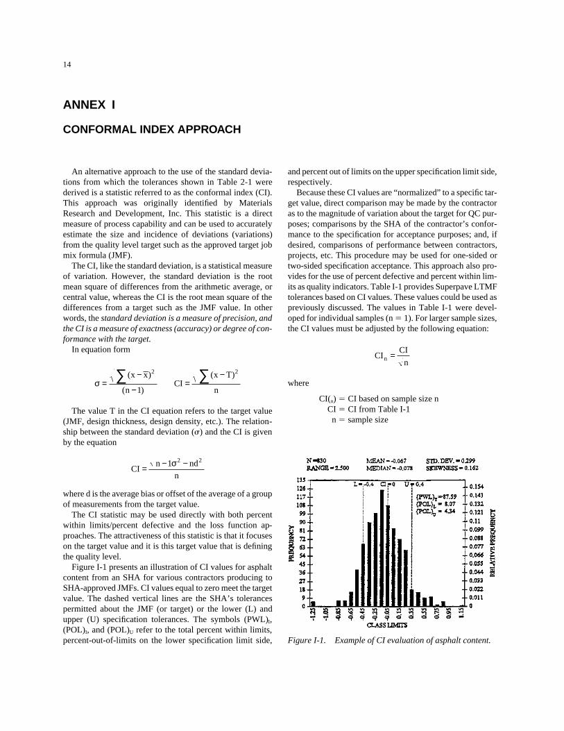
Figure I-1 presents an illustration of CI values for asphaltcontent from an SHA for various contractors producing toSHA-approved JMFs. CI values equal to zero meet the targetvalue. The dashed vertical lines are the SHA’s tolerancespermitted about the JMF (or target) or the lower (L) andupper (U) specification tolerances. The symbols (PWL)I,(POL)I, and (POL)U refer to the total percent within limits,percent-out-of-limits on the lower specification limit side,
CIn nd
n= − −1 2 2σ
σ =−
−=
−∑ ∑( )
( )
( )x x
nCI
x T
n
2 2
1
and percent out of limits on the upper specification limit side,respectively.
Because these CI values are “normalized” to a specific tar-get value, direct comparison may be made by the contractoras to the magnitude of variation about the target for QC pur-poses; comparisons by the SHA of the contractor’s confor-mance to the specification for acceptance purposes; and, ifdesired, comparisons of performance between contractors,projects, etc. This procedure may be used for one-sided ortwo-sided specification acceptance. This approach also pro-vides for the use of percent defective and percent within lim-its as quality indicators. Table I-1 provides Superpave LTMFtolerances based on CI values. These values could be used aspreviously discussed. The values in Table I-1 were devel-oped for individual samples (n � 1). For larger sample sizes,the CI values must be adjusted by the following equation:
where
CI(n) � CI based on sample size nCI � CI from Table I-1
n � sample size
CICI
nn =
Figure I-1. Example of CI evaluation of asphalt content.
14
15
TABLE I-1 Superpave LTMF tolerances based on CI values (mixture composition and gyratory properties)
ANNEX II
STRATIFIED RANDOM SAMPLING APPROACH
SCOPE
This method outlines the procedures for selecting sam-pling sites in accordance with accepted random samplingtechniques. Random sampling is the selection of a sample insuch a manner that every portion of the material or construc-tion to be sampled has an equal chance of being selected asthe sample. It is intended that all samples, regardless of size,type, or purpose, shall be selected in an unbiased manner,based entirely on chance.
SECURING SAMPLES
Samples shall be taken as directed by the QC representa-tive for QC purposes and the state highway representative foracceptance purposes.
Sample location and sampling procedure are as importantas testing. It is essential that the sample location be chosen inan unbiased manner.
RANDOM NUMBER TABLE
For test results or measurements to be meaningful, it isnecessary that the sublots to be sampled or measured beselected at random, which means using a table of randomnumbers. The following table of random numbers has beendevised for this purpose. To use the table in selecting samplelocations, proceed as follows.
Determine the lot size (continuous production for QC atHMA plant) and stratify the lot into a number of sublots perlot for the material being sampled.
For each lot, use consecutive two-digit random numbersfrom Table II-1. For example, if the specification specifiesfive sublots per lot and the number 15 is randomly selected asthe starting point from column X (or column Y) for the firstlot, numbers 15 to 19 are the five consecutive two-digit ran-dom numbers. For the second lot, another random startingpoint, number 91 for example, is selected and the numbers 91to 95 are used for the five consecutive two-digit randomnumbers. The same procedure is used for additional lots.
For samples taken from the roadway, use the decimal val-ues in column X and column Y to determine the coordinatesof the sample locations.
In situations where coordinate locations do not apply (i.e.,plant samples, stockpile samples, etc.), use those decimalvalues from column X or column Y.
16
DEFINITION OF TERMS
lot: An isolated quantity of a specified material from a sin-gle source or a measured amount of specified constructionassumed to be produced by the same process.
sublot: A portion of a lot, the actual location from which asample is taken. The size of the sublot and the number ofsublots per lot for acceptance purposes are specified in thespecifications.
THE RANDOM SAMPLE
A random table is a collection of random digits. The ran-dom numbers that are presented in this annex are shown in atwo-place decimal format. Note that there are two columns,labeled X and Y. The numbers in either column can be usedto locate a random sample when only a single dimension isrequired to locate the sample (e.g., time, tonnage, and units).When two dimensions are required to locate the sample, thenumber in the X column is used to calculate the longitudinallocation, and the number in the Y column is used to calculatethe transverse location. In the Y column, each number is pre-ceded by L or R, designating that the sample increment is tobe located transversely from the left or right edge of the pave-ment. Figure II-1 illustrates the procedure.
The following examples demonstrate the use of the ran-dom sampling technique under various conditions.
EXAMPLE 1: SAMPLING BY TIME SEQUENCE
Assume that HMA for use in paving is to be sampled todetermine the percent asphalt. It will be sampled at the placeof manufacture. The task is to select a random sampling planto distribute the sampling over the half day or the full day,whichever is more applicable. Assume that the lot size is aday’s production and that five samples are required fromeach lot. The plant is assumed to operate continuously for 9 h (beginning at 7:00 am and continuing until 4:00 pm) withno break for lunch.
1. Lot size. The lot size is a day’s production. The plantstarts at 7:00 am and stops at 4:00 pm. Hence, the lotsize is 9 h of production.
2. Sublot size. Stratify the lot into five equal sublots,because five samples are required. To accomplish this,select five equal time intervals during the 9 h that theplant is operating.
TABLE II-1 Random positions in decimal fractions (two places)
3. Sublot samples. Next, choose five random numbersfrom the random number table. The first block ran-domly selected is reproduced below.
Sequence number X Y
12 0.57 R 0.4613 0.35 R 0.6014 0.69 L 0.6315 0.59 R 0.6816 0.06 L 0.03
The selected random numbers taken from the X columnare 0.57, 0.35, 0.66, 0.56, and 0.06. To randomize the sam-pling times within each sublot, the time interval (108 min)computed in Step 2 is used. This time interval is multipliedby each of the five random numbers previously selected:
These times are added to the starting times for each sublot.This results in the randomized time at which the sample is tobe obtained. The sampling sequence is as follows:
Sublot SamplingNumber Time
1 7:00 am � 62 min � 8:02 am2 8:48 am � 38 min � 9:26 am3 10:36 am � 75 min � 11:51 am4 12:24 pm � 64 min � 1:28 pm5 2:12 pm � 6 min � 2:18 pm
18
The random sampling times are shown in Figure II-2. Ifproduction is not available at the indicated time, a sampleshould be obtained at the first opportunity after the indicatedtime.
Sampling on a time basis is practical only when theprocess is continuous. Intermittent processes obviously pre-sent many difficulties.
EXAMPLE 2: SAMPLING BY MATERIAL TONNAGE
HMA for use in paving must be sampled to determine theasphalt content. The specifications define the lot size as 5,000tons and state that five samples must be obtained from the lot.The sampling is to be done from the hauling units at the man-ufacturing source. The total tonnage for the project is 20,000tons.
This solution follows the same basic pattern as the solu-tion given for the previous example. First, identify the lotsize and then determine the number of lots, sublot size, and,finally, the point at which samples will be obtained.
1. Lot size and number of lots. The lot size is 5,000 tons.Because there are 20,000 tons of bituminous mixrequired for the project, the total number of lots is
2. Sublot size. Stratify each lot into five equal sublots. Thesublot size is
The relationship between lot and sublot size is shownin Figure II-3.
3. Sublot samples. The number of samples per lot is five,one per sublot. Five random numbers are thereforeselected from the table of random numbers. Again, thefirst block of numbers from the random number table isreproduced below. This time, a different set of numbersis selected
Sublot sizetons lot
sublots lottons sublot= =5 000
51 000
, /
/, /
Number of lotstons
tons lotlots= =20 000
5 0004
,
, /
Figure II-1. Determination of sample location usingrandom numbers.
Figure II-2. Sublot sample times based on time sequence.
Sublot time ervalh lot h
sublots lot
sublot
int( / )( min/ )
/
min/
=
=
9 60
5
108
Sequence number X Y
67 0.93 R 0.1768 0.40 R 0.5069 0.44 R 0.1570 0.03 L 0.6071 0.19 L 0.37
The selected random numbers this time are from the Ycolumn (disregard the L or R): 0.17, 0.50, 0.15, 0.60,and 0.37. These numbers are then multiplied by each ofthe five sublots as follows:
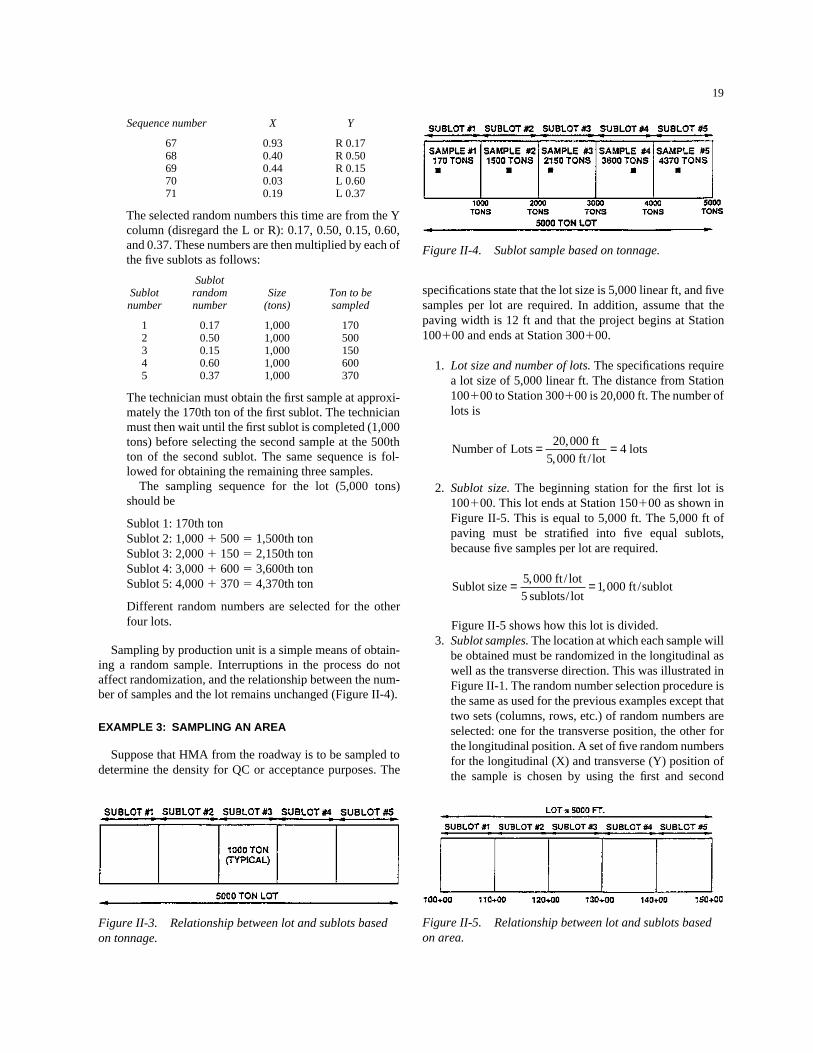
SublotSublot random Size Ton to benumber number (tons) sampled
The technician must obtain the first sample at approxi-mately the 170th ton of the first sublot. The technicianmust then wait until the first sublot is completed (1,000tons) before selecting the second sample at the 500thton of the second sublot. The same sequence is fol-lowed for obtaining the remaining three samples.
The sampling sequence for the lot (5,000 tons)should be
Different random numbers are selected for the otherfour lots.
Sampling by production unit is a simple means of obtain-ing a random sample. Interruptions in the process do notaffect randomization, and the relationship between the num-ber of samples and the lot remains unchanged (Figure II-4).
EXAMPLE 3: SAMPLING AN AREA
Suppose that HMA from the roadway is to be sampled todetermine the density for QC or acceptance purposes. The
19
specifications state that the lot size is 5,000 linear ft, and fivesamples per lot are required. In addition, assume that thepaving width is 12 ft and that the project begins at Station100�00 and ends at Station 300�00.
1. Lot size and number of lots. The specifications requirea lot size of 5,000 linear ft. The distance from Station100�00 to Station 300�00 is 20,000 ft. The number oflots is
2. Sublot size. The beginning station for the first lot is100�00. This lot ends at Station 150�00 as shown inFigure II-5. This is equal to 5,000 ft. The 5,000 ft ofpaving must be stratified into five equal sublots,because five samples per lot are required.
Figure II-5 shows how this lot is divided.3. Sublot samples. The location at which each sample will
be obtained must be randomized in the longitudinal aswell as the transverse direction. This was illustrated inFigure II-1. The random number selection procedure isthe same as used for the previous examples except thattwo sets (columns, rows, etc.) of random numbers areselected: one for the transverse position, the other forthe longitudinal position. A set of five random numbersfor the longitudinal (X) and transverse (Y) position ofthe sample is chosen by using the first and second
Sublot sizeft lot
sublots lotft sublot= =5 000
51 000
, /
/, /
Number of Lotsft
ft lotlots= =20 000
5 0004
,
, /
Figure II-3. Relationship between lot and sublots basedon tonnage.
Figure II-4. Sublot sample based on tonnage.
Figure II-5. Relationship between lot and sublots basedon area.
blocks of random numbers from the random numbertable. These are reproduced as follows:
Sequence number X Y
37 0.41 L 0.1038 0.28 R 0.2339 0.22 L 0.1840 0.21 L 0.9441 0.27 L 0.52
The numbers are selected from both X and Y columns.Include the L or R in the Y column:
Longitudinal (X): 0.41 0.28 0.22 0.21 0.27Transverse (Y): L 0.10 R 0.23 L 0.18 L 0.94 L 0.52
These X and Y random numbers are multiplied by thesublot length and paving width respectively, as shownbelow:
Sublot 1 (starting Station 100�00)Coordinate X � 0.41 � 1,000 ft � 410 ftCoordinate Y � 0.10 � 12 ft � 1.2 ft
Sublot 2 (starting Station 110�00)Coordinate X � 0.28 � 1,000 ft � 280 ftCoordinate Y � 0.23 � 12 ft � 2.8 ft
Sublot 3 (starting Station 120�00)Coordinate X � 0.22 � 1,000 ft � 220 ftCoordinate Y � 0.18 � 12 ft � 2.2 ft
20
Sublot 4 (starting Station 130�00)Coordinate X � 0.21 � 1,000 ft � 210 ftCoordinate Y � 0.94 � 12 ft � 11.3 ft
Sublot 5 (starting Station 140�00)Coordinate X � 0.27 � 1,000 ft � 270 ftCoordinate Y � 0.52 � 12 ft � 6.2 ft
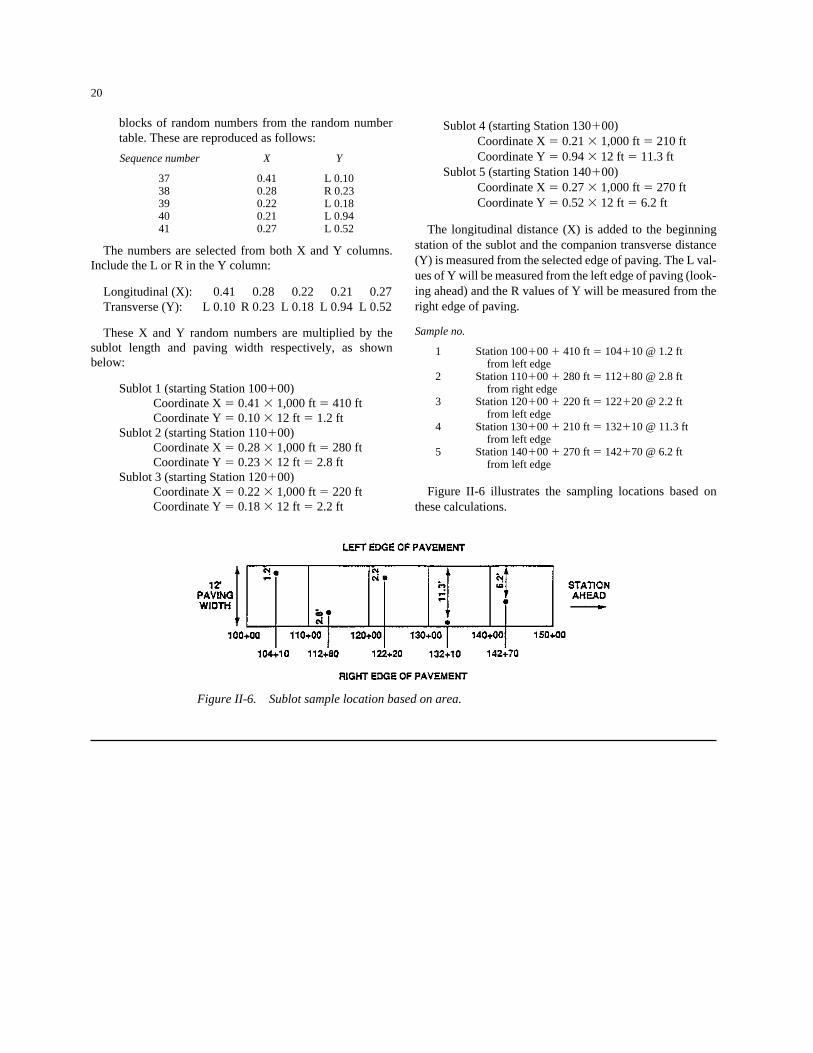
The longitudinal distance (X) is added to the beginningstation of the sublot and the companion transverse distance(Y) is measured from the selected edge of paving. The L val-ues of Y will be measured from the left edge of paving (look-ing ahead) and the R values of Y will be measured from theright edge of paving.
Sample no.
1 Station 100�00 � 410 ft � 104�10 @ 1.2 ft from left edge
2 Station 110�00 � 280 ft � 112�80 @ 2.8 ft from right edge
3 Station 120�00 � 220 ft � 122�20 @ 2.2 ft from left edge
4 Station 130�00 � 210 ft � 132�10 @ 11.3 ft from left edge
5 Station 140�00 � 270 ft � 142�70 @ 6.2 ft from left edge
Figure II-6 illustrates the sampling locations based onthese calculations.
Figure II-6. Sublot sample location based on area.
21
ANNEX III
STATISTICAL CONTROL CHARTS
The process control procedure recommended is the use ofcontrol charts, particularly statistical control charts. Controlcharts provide a means of verifying that a process is in con-trol. It is important to understand that statistical controlcharts do not get or keep a process under control. Theprocess must still be controlled by the plant or constructionpersonnel. Control charts simply provide a visual warningmechanism to identify when the Contractor or material sup-plier should look for possible problems with the process.
Variation of construction materials is inevitable andunavoidable. The purpose of control charts, then, is not toeliminate variability but to distinguish between the inherent orchance causes of variability and a system of assignablecauses. Chance causes (sometimes known as common causes)are a part of every process and can be reduced but generallynot eliminated. Assignable causes (sometimes known as spe-cial causes) are factors that can be eliminated, thereby reduc-ing variability. Chance causes are something that a Contrac-tor or material supplier must learn to live with. They cannotbe eliminated, but it may be possible to reduce their effects.The second cause of variation, assignable causes, can createmajor problems. However, assignable causes can be elimi-nated if they can be identified. Examples of assignable causesmight be the gradation for an aggregate blend going out ofspecification because of a hole in one of the sieves or becausethe cold feed conveyor setting is incorrectly adjusted.
The statistical control charts enable the Contractor to dis-tinguish between chance and assignable causes. Based onstatistical theory, construction materials, when under pro-duction control, exhibit a “bell-shaped” or normal distribu-tion curve.
The data, therefore, can be assumed to be within �3� ofthe mean or target when the process is in control and onlychance causes (variability that the Contractor cannot con-trol) are acting on the system. Statistical control charts foraverage or means rely on the fact that, for a normal distribu-tion, essentially all the values fall within �3� from the mean.The normal distribution can be used because the distributionof sample means is normally distributed.
A statistical control chart can be viewed as a normal distri-bution curve on its side (Figure III-1). For a normal curve,only about 0.27 percent (1 of 370) of the measurements shouldfall outside �3� from the average or mean. Therefore, controllimits (indicating that an investigation for an assignable causeshould be conducted) are set at �3�x– and �3�x–
A statistical control chart includes a target value, upperand lower control limits, and a series of data points that are
plotted. The target is based on the population or productionmean and the control limits are established from the popula-tion or production standard deviation as shown in Figure III-2.
There are many forms of statistical control charts, but twoforms are most practical and useful for construction materi-als and processes. These are the control charts for means oraverages (commonly referred to as x, called x-bar chart) andthe control chart for ranges (commonly referred to as an R-chart). The x-chart is typically used to control the produc-tion process about the average or target value. The R-chartconsiders the variability of the material and preventsextremely large positive and negative results from cancelingout and not being detectable on the control chart for meansor averages. The range, which is the easiest measure ofspread to use in the field, is usually used in place of the stan-dard deviation.
Population or production parameters (i.e., averages andranges) are either known (or specified) or are estimated fromthe early stages of the production process. In most cases, thelatter is true. It is not a good idea for a producer to use themean, range, or standard deviation that were specified or
Figure III-1. Example of statistical control chart.
Figure III-2. Elements of statistical control chart.
used by the highway agency when it developed the specifi-cation limits. The mean, range, and standard deviation of aproducer’s process are independent of the specification lim-its; they are established by the process capability.
When the mean and standard deviation are not known (thisis usually the case), they are estimated by the grand averageor mean (X�) and the average range (R– ). The grand average
22
or mean is defined as the average value of a group of aver-ages. The average range is defined as the average of individ-ual range values. For the X
–-chart, the grand mean becomes
the target value; for the R-chart, the average range becomesthe target value.
The following formulas are used to construct the twocontrol charts:
TABLE III-1 Factors for statistical control charts
TABLE III-2 Data for demonstration example
X—-chart
R-chart
The factors A2, D3, and D4 are obtained from Table III-1for the appropriate sample size n. Note that the sample sizeis always greater than 1. For each QC test, the samples aregrouped to form a subgroup of 2 or larger.
EXAMPLE: CONTROL CHARTS WHEN MEANAND STANDARD DEVIATION ARE UNKNOWN
The data shown in Table III-2 will be used to illustrate thecalculation for a control chart when the population parame-ters are unknown and are estimated from the early productionprocess. The table contains the gradation results for percentpassing the 4.75-mm (No. 4) sieve for 40 production days(four tests per day). The average and range of the first 20 sub-groups are used to estimate the mean and standard deviationof the population. When this is done
Having found these values, the UCL and LCL can be cal-culated from the formulas previously identified. Note that thevalues for A2, D3, and D4 are for a sample subgroup of n � 4because four samples are used to find each average, X—, andrange, R.
X—-chart
UCL X A RLCL X A R
Target Value X
= + × = + × == − × = − × =
= =
( . ( . . ) .( . ( . . ) .
.
2
2
18 3 0 73 4 2 21 418 3 0 73 4 2 15 2
18 3
X
R
= + + + + = =
= + + + + = =
18 4 18 0 18 4 16 4
20
365 9
2018 3
2 1 4 1 4 7 3 9
20
83 6
204 2
. . . . ..
. . . . ..
K
K
Upper Control Limit UCL D R
Lower Control Limit LCL D R
( )
( )
= ×
= ×4
3
Upper Control Limit UCL X A R
Lower Control Chart LCL X A R
( ) ( )
( ) ( )
= + ×
= − ×
2
2
23
R-chart
Once the target value and control limits are established,the control charts can be constructed with the data in TableIII-2. Figures III-3 and III-4 illustrate the X
–and R-charts for
the data.
UCL D R
LCL D R
T et Value R
= × = × =
= × = × =
= =
4
3
2 28 4 2 9 6
0 0 4 2 0 0
4 2
. . .
. . .
arg .
Figure III-3. X—
-chart for percent passing 4.75-mm (No. 4)sieve.
Figure III-4. R-chart for percent passing 4.75-mm (No. 4)sieve.
CHAPTER 3
GUIDELINES FOR ADJUSTING THE PRODUCTION AND PLACEMENT OF SUPERPAVE-DESIGNED HMA
This chapter contains guidelines for solving problems thatoccur during production of the HMA designed in accordancewith the Superpave method. These problems can be classi-fied as noncomplying gradation and HMA test properties,undesirable placement characteristics, and undesirable char-acteristics of the finished pavement. Solutions often requireadditional testing, analysis, and adjustments. These guide-lines are based on the National Asphalt Pavement Associa-tion’s (NAPA) publication QIP-97, “Quality Control forHot-Mix Plant and Paving Operations.” These practices werefollowed on the NCHRP Project 9-7 construction projectsand are applicable to the Superpave-designed HMA produc-tion and placement operations.
3.1 NONCOMPLYING GRADATION TESTS
3.1.1 Incoming Aggregates
If a reliable estimate of the actual gradation of the differ-ent sizes of aggregates indicates that it will not be possible toproduce a mixture meeting the Superpave mix specificationsand the LTMF requirements, and if these requirements can-not be modified, one of the following courses of action issuggested:
• Compute an acceptable theoretical combined gradationbased on wasting some portions of the delivered mater-ial.
• Check to see if blending an additional size of aggregatewith delivered material will produce an acceptable com-bined gradation.
• Reject aggregate and procure material from an alterna-tive source.
3.1.2 Combined Hot Bin Aggregate
If the combined gradation of the hot bin aggregate does notfall within the LTMF tolerances, the following proceduresare recommended:
• Resample fine aggregate bin and make gradation tests tocheck previous sampling.
24
• If resampling results check closely with previous sam-pling, recompute the gradation to see if changing binweights will produce an acceptable combined gradation.If this is not possible because of a lack of one or moresieve sizes in the raw aggregates, follow the proceduresdescribed previously for incoming aggregates.
• If resampling does not check with previous sampling1. Check sampling methods to make sure that the sam-
ple truly represents bin contents,2. Make a series of tests on the bins where variations in
gradation occur to determine if differences are due toa. Hole in the screen.b. Temporary overrun into the bin caused by crowd-
ing the plant and exceeding the capacity of thescreen.
c. Continued overrun caused by blinding of thescreen; this condition occurs when particles ofaggregate plug up the openings in the screen;blinding can usually be avoided or reduced bysubstituting a slotted screen or one with slightlylarger openings.
d. Problems in the cold feed; check cold feed forproportions and consistency; moisture in fineaggregate can cause inconsistent feedings.
3.2 NONCOMPLYING HMA TEST RESULTS
3.2.1 Air Voids Above or Below Specifications
The percent of air voids in the compacted HMA depends onthe percent of voids in the mineral aggregate and the percentof asphalt. When the percent of air voids is too high or too low,placement problems will occur. The standard deviation in anormal determination of percent air voids is about 1 percent.This means that at least six different samples of HMA shouldbe tested and averaged to determine if the percent air voids iswithin the specified range. The usual range is 3 to 5 percent. Ifthe air voids are not within the Superpave mix design specifi-cations, the following actions should be taken:
• Check that the correct value of maximum theoreticalspecific gravity has been used in the computations; small
variations in the maximum theoretical specific gravitycan cause significant differences in the calculated airvoids content.
• Check the procedure used to determine the bulk specificgravity of the specimen.
• Check that the mix sampled is representative; if theasphalt content of the sample is not in agreement withthe LTMF, the voids’ properties will not match the mixdesign.
• If all checks show that correct values are being used, theasphalt content may be adjusted to produce an averageof 4 percent (or other specified value) of air voids.
• If it is not possible to change the asphalt content, theVMA must be adjusted by changing the gradation asdescribed in the following paragraphs.
3.2.2 VMA
The VMA are the bulk volume of the compacted pavingminus the volume of the aggregate determined from its bulkspecific gravity. It can also be viewed as the volume of airvoids plus the volume of effective asphalt binder. It isexpressed as a percent of the bulk volume of the compactedmix.
The VMA is very important in the Superpave mix designmethod, particularly for wearing and surface course mix-tures. Space must be left in the compacted mixture to allowroom for the specified asphalt content and air voids. Theunfilled voids (air voids) must be present to allow room forthe asphalt to expand and for compaction under traffic loadsduring periods of hot summer temperatures. This will pre-vent the asphalt from flushing to the surface and causing themixture to become plastic.
The Superpave mix design procedure aims to producewearing course mixes that have, after traffic compaction,about 4 percent by volume of air voids, with about 75 or 80percent of the VMA filled with asphalt binder. To meet theseconditions, the Superpave minimum VMA design require-ments are based on the nominal maximum aggregate size.Dense gradations that produce mixes below these values donot have enough room for the asphalt binder. This is partic-ularly a problem when natural sand and bank-run gravel areused as aggregates. Mixes made with these rounded particleshave been observed to flush and ravel at the same time. Thefine particles collected by baghouse dust collectors can alsoreduce the air voids content and cause a low value of voidsin the mineral aggregate.
• Roundness or lack of angularity of aggregate particles;• Gradation of coarse and fine aggregate; and• Amount of filler or material passing the No. 200 sieve.
25
3.2.3 Increasing VMA
The percent of VMA can be increased by any of the fol-lowing:
• Using more angular crushed aggregate in the mix. Sub-stituting manufactured fine aggregate or screenings pro-duced by crushing is usually effective if the fractionpassing the 0.075-mm (No. 200) sieve is controlled.
• Decreasing the percentage of material passing the 0.150-mm (No.100) sieve by wasting all or part of the dustreturned from the dust collector. Reducing the percentof minus 0.150-mm (No.100) material will increase theVMA.
• Increasing the amount of 4.75-mm (No. 4) to 0.150-mm(No. 100) aggregate. This may require an increase in theamount of asphalt binder.
• Moving gradation away from the maximum density line0.45 power curve.
3.2.4 Decreasing VMA
The percent of VMA can be decreased by any of the fol-lowing:
• Use of rounded or cubical coarse aggregate;• Use of a fine aggregate consisting of natural sand with
rounded particles;• Increasing the amount of filler in the mixture (Note:
there is a practical limit on the amount passing the0.075-mm (No. 200) sieve that can be tolerated in a mix;the rule of thumb is that the percent of filler by weightshould not exceed approximately 1.2 times the percentof effective asphalt by weight).
3.2.5 VFA
The percent of VFA affects the durability and flexibility ofthe pavement. A good target value is about 75 percent. For amix designed for a wearing course for normal highway traf-fic, values of less than 65 percent can cause premature orexcessive hardening of the asphalt binder in the pavement,cracking, and even raveling. Values greater than 85 percentcan lead to flushing, shoving, and rutting. The optimum VFAcan be obtained when the air voids content is 4 percent andthe VMA is that specified in the Superpave mix designmethod for the nominal maximum aggregate size. Adjust-ments in the percent of air voids and VMA are made by themethods discussed in the preceding paragraphs.
3.3 NONCOMPLYING FIELD DENSITY TESTS
Studies have shown that the density of an asphalt pavingcourse is usually highest in the center of the lane, because of
overlapping roller coverages. It is lower at the edges of thelane because of fewer coverages. This causes a variation indensity when nuclear density or pavement cores are taken atrandom locations across the lane.
If an accurate measurement of pavement density fallsbelow the specified percent of reference density, it may bedue to the following conditions:
1. Use of a maximum theoretical density based on inac-curately measured or assumed specific gravities ofaggregates and asphalt binder. The maximum theoreti-cal specific gravity of the mixture as determined byprocedures described in AASHTO Method ASTMD2041 (the “Rice Method”) is a way to test the totalmix rather than base the result on the properties of theindividual aggregates.
2. Use of a reference density based on gyratory-compacted specimens that were overcompacted ormade at too high a temperature.
3. Insufficient field compaction caused by underweightrollers, the wrong type of roller, or insufficient cover-ages.
4. Rolling at too low a temperature.5. Difficulties in compacting tough mixtures. These
HMA may have a high strength or too much filler inrelation to the amount and properties of the asphaltbinder in the mix. The resulting pavement may havehigh air voids content.
6. Presence of clay dust in the material passing the 0.075-mm (No. 200) sieve in the mixture.
7. Compacting against soft and yielding bases and sub-bases. The pavement cannot be compacted if the mate-rial beneath it is soft and yielding. The specified den-sity and the deflection of the surface on which HMApavement is to be constructed should be checked beforestart of laydown.
8. Tender mix.
3.4 MISCELLANEOUS IRREGULARITIES IN PAVEMENT
3.4.1 Checking and Cracking of NewlyConstructed Pavement
This condition is usually caused by improper rolling tech-niques. A competent roller operator will avoid the followingsituations:
1. Overrolling a tender mix;2. Rolling a mat that has cooled on the surface but is plas-
tic underneath or rolling when the roller wheels are toocold;
26
3. Rolling a dense mix while it is too hot;4. Overrolling when the base deflects;5. Rolling too fast, turning abruptly, or starting and stop-
ping abruptly; and6. Using a highly temperature-susceptible asphalt binder.
3.4.2 Shoving of the Compacted Pavement
Shoving of paving mixtures during construction may becaused by
1. Using a too-heavy roller;2. Operating a breakdown roller when drive wheels are
not toward the paver;3. Rolling a plastic mix, caused by temperatures that are
too high or by a mix design with too high a VFA value;and
4. Moisture in mix.
3.4.3 Raveling in the Finished Pavement
Raveling may be caused by
1. Asphalt content too low;2. Excessive segregation while loading trucks;3. Rolling at too low a temperature, parts of load too
cold;4. Rolling a wet mat, too much water on roller wheels;5. Dirt coating on aggregates, incomplete coating of ag-
gregates, unsuitable filler; and6. Excessive hardening of asphalt, caused by too high
a temperature in one or more of the aggregate hot bins.
3.4.4 Tender Pavements
Tender HMA will push and shove under the roller. It willtake an unusually long time to set and will scuff or scar underturning wheels. Tender HMA and pavement are caused bythe following:
1. Slow setting asphalt (slow to develop strength neededduring construction);
2. Contaminated asphalt/cement;3. Too much diesel oil (used as release agent) in the bot-
tom of trucks;4. Too much asphalt binder in the mix;5. Too little asphalt binder in the mix;6. Too much dust in a batch; and7. Excessive moisture in a dense hot mix.
27
CHAPTER 4
A TRAINING COURSE TO IMPLEMENT QC/QA PLANS FORPRODUCTION AND PLACEMENT OF SUPERPAVE-DESIGNED HMA
4.1 INTRODUCTION
The training course developed through NCHRP Project 9-7 should assist agencies, contractors and others in imple-menting the Superpave QC/QA recommendations from theproject. The training package was developed with severaldifferent modules so that training could be tailored to the spe-cific needs of the audience. The modules are as follows:
Module I: Introduction to the Training CourseModule II: Superpave Mix Design and AnalysisModule III: QC/QA ConceptsModule IV: Plant ActivitiesModule V: Laboratory ActivitiesModule VI: QC Plan for Superpave-Designed HMAModule VII: QA Plan for Superpave-Designed HMA
4.2 OVERVIEW OF TRAINING COURSE
The detailed outline of the training course presented belowillustrates all the various topics that are covered and providesinsight on how to use the modular structure of the courseeffectively.
Module I. Introduction to the Training CourseCourse objectivesCertification
Module II. Superpave Mix Design and AnalysisIntroduction to the Superpave mixdesign and analysis systemPerformance-graded binder testing andselectionAggregate testing and selectionVolumetric mix design conceptsSuperpave volumetric mix designprocessSuperpave mix analysis concepts
Module III. QC/QA ConceptsDefinitions of QC/QAStatistical backgroundRandomized sampling techniquesLot/sublot concepts
Statistical control chartsPWLConformal indices (optional)
Module IV. Plant ActivitiesPlant calibrationPlant gradation controlsMix temperature requirementsProper sampling techniquesPlant adjustments
Module V. Laboratory ActivitiesLaboratory testing equipment calibrationFrequency and sequence of testsTesting protocols and proceduresTest results and interpretations
Module VI. QC Plan for Superpave-Designed HMA
Part IBackground/objectives of NCHRPProject 9-7Development and assumptions ofQC/QA proceduresDevelopment of field shear testingdevicesContractor responsibilitiesDevelopment of tolerance limitsApplication of statistical control chartsGyratory procedures for QC/QA
Part IIBinder certificationEstablishing the LTMFSelection of properties for controlLaboratory verification of LTMFField verification of LTMFMix production QCIn-place QCCourses of action throughout QCprocess
Module VII. QA Plan for Superpave-Designed HMAAgency responsibilitiesPWL approachBinder acceptance
Specification/tolerance limits foracceptanceSelection of properties for acceptanceAcceptance of LTMF/JMF (lab, field,mix, in-place)Comparison of QC and QA data-disputeresolution
28
This chapter includes the slides and instructor’s notes forModules VI and VII. Appendix A contains the slides forModules I through V. The instructors notes and slides weredeveloped assuming that those presenting the course mater-ial have a thorough knowledge of the Superpave mix designand analysis system and an understanding of the statisticalconcepts related to QC and QA procedures.
Slide 1 This module will provide information detailingthe basis for the QC Plan developed for Super-pave-designed mixes. Superpave QC/QA neededto be developed to help implement the overallSuperpave system. The Superpave systemincludes mixture design, mixture analysis, andproduction/construction.
Slide 2 After the end of the SHRP research effort, theneed for a Superpave QC/QA Plan was identifiedby both government and industry groups. NCHRPProject 9-7 was awarded in March 1993 to addressthis need.
Slide 3 The objectives established for this contract wereto establish procedures and develop equipment forQC/QA at the plant and lay down as well asdevelop a mechanism for training technicians andengineers on Superpave QC/QA procedures.
Module VI — Superpave Quality Control (QC) Plan: Part 1 29
Module VI — Part 1: Slide 1
Module VI — Part 1: Slide 2
Module VI — Part 1: Slide 3
Slide 4 There are several reasons for ensuring qualitythroughout the production of HMA, but the bot-tom line comes down to money. Generally, thecontractors make more money when they producea quality product and highway agencies (i.e., thetaxpayers) save money in future maintenancecosts if quality is built into pavements.
Slide 5 Some of the basic principles of HMA QC statethat QC should be based on measurements that aretimely and easy to perform. The contractor andclient do not want to wait a long time before theyfind out that the HMA does not conform torequired specifications. Extended waits will costsignificant amounts of money.
Slide 6 QC also should be based on equipment that isappropriate for field use and the QC processshould also be simple and easy to apply. Agenciesdo not want to spend large sums of money toobtain QC equipment, nor do they want to have tohire additional technicians with specialized skillsor training. Agencies will want to train existingemployees.
30 Module VI — Superpave Quality Control (QC) Plan: Part 1
Module VI — Part 1: Slide 4
Module VI — Part 1: Slide 5
Module VI — Part 1: Slide 6
Slide 7 There are three basic areas where variation can beintroduced into the QC process. They are sam-pling, testing, and material variability. A QC Planthat is developed correctly should account foreach of these areas.
A QC Plan should also differentiate betweenHMA production and construction.
Production: material coming out of the plant. Isit correct?
Construction: material being placed on theroadway. Is it correct?
Finally, a QC plan also should be based on per-formance-related properties or properties that canbe used to determine how a mixture will perform ifa deviation occurs from the original mix design(i.e., poor QC). Performance-related specificationsare typically based on these types of properties andare important when pay factors are involved.
Slide 8 There are essentially four points at which QCshould occur throughout the HMA production/construction process. Points one and two are theQC processes that occur with the materials used inthe production of HMA mixtures. Binder (orasphalt cement) should be checked to make surethat it conforms to the performance-graded (PG)properties determined during the mix designprocess. The aggregates should also be checked toensure that the blended materials meet the grada-tion requirements (or other properties as identifiedby the QC Plan) determined in the initial mixdesign.
The third point in the QC process occurs afterthe materials have been mixed through the plantproduction process. Various properties of theHMA mix should conform, within specified toler-ances, to those values established in the mix designprocess. These properties traditionally have in-cluded air voids, percent asphalt, VMA, and sometype of strength parameter. The final point in theQC process is the determination of the in-placeproperties. This occurs after the HMA has beenplaced by a lay down machine and compacted by aseries of passes of heavy rollers. Typically, in-place compaction is checked against some mini-mum value of air voids that must be attained by theuse of nondestructive testing (NDT) methods. TheNDT values are verified with a small sample of in-place cores (or destructive sampling).
Slide 9 Several devices that can be used in the QC processwere evaluated or developed in the NCHRP Proj-ect 9-7 research effort. These products includedevices for performing QC on binders, aggre-gates, and mixtures.
Module VI — Superpave Quality Control (QC) Plan: Part 1 31
Module VI — Part 1: Slide 7
Module VI — Part 1: Slide 8
Module VI — Part 1: Slide 9
Slide 10 The SDR is a device that can be used to quicklydetermine the quality of asphalt binders at theplant lab. The device at first glance looks like thering and ball test but it is very different from thatdevice because the SDR operates only in the elas-tic region of the material (i.e., all deformation isrecoverable). In the SDR test an indentor ofknown weight is placed on a sample at a giventemperature for a given time period. The dis-placement of the sample is measured and variousproperties of the sample are determined.
Slide 11 The parameters determined from the test includethe shear modulus and the phase angle.
Slide 12 The SDR can be used as a quick field QC test ofPG binders because the parameters determinedfrom the SDR include those properties used in thePG determination for asphalt binders using theother SHRP binder characterization equipment.
32 Module VI — Superpave Quality Control (QC) Plan: Part 1
Module VI — Part 1: Slide 10
Module VI — Part 1: Slide 11
Module VI — Part 1: Slide 12
Module VI — Part 1: Slide 15
Slide 13 The SDR test is conducted at three different tem-peratures with various times to deformation andindentation ball weights. The combination of theresults can be used to generate the material prop-erties for the sample.
Slide 14 The sample’s master curve is generated by usingthe results from the various temperatures.
Slide 15 The aggregate video grader can be used to deter-mine the blended gradation of the aggregates usedfor the HMA. The video grader can either be usedin-line on the cold feed aggregate conveyor or inthe lab with the portable unit. The video graderprovides quick gradation results comparable tothe results of traditional sieve analysis.
Module VI — Superpave Quality Control (QC) Plan: Part 1 33
Module VI — Part 1: Slide 13
Module VI — Part 1: Slide 14
Slide 16 The video grader operates with an image analyzerexamining the aggregate as it passes by a high-speed video camera. The aggregate free-falls pastthe video camera and the image is analyzed bycomputer software that determines the size frac-tion gradation.
Slide 17 The video grader provides results comparable tothose determined by the more traditional sieveanalysis methods and provides the results morequickly. This is especially important for QC activ-ities when time is of the essence.
Slide 18 Devices were also investigated and developed thatprovide engineering properties that can be used topredict pavement performance. These deviceswere specifically developed for field control andare easy to operate, low cost, and portable.
34 Module VI — Superpave Quality Control (QC) Plan: Part 1
Module VI — Part 1: Slide 16
Module VI — Part 1: Slide 17
Module VI — Part 1: Slide 18
Slide 19 The Field Shear Tester (FST) was developed underthe technical direction of the NCHRP Project 9-7research personnel. This device is considered aderivative of the Superpave Shear Tester (SST)developed under the SHRP A-003 contract be-cause it has the ability to run tests and generateproperties similar to those from the SST. However,there are some significant differences betweenthese two devices that must be recognized.
First, the loading configuration of the FST issimilar to a direct shear load as opposed to thesimple shear loading of the SST. The loadingconfiguration for the FST was developed withsimplicity in mind. It was believed by the NCHRP9-7 researchers that sample preparation for a fieldcontrol device should be minimal. To achievethis, the loading mechanism shown in the slidewas developed. Second, control of the closed-looppneumatic system is handled by the loadingmechanism as opposed to the deformation controlthat the SST uses for many tests. The deformationmeasuring device of the FST is different from theSST measuring device, again for simplicity. Thelinear variable differential transformer is notphysically attached to the specimen and thus is notrecommended as a control mechanism becauseslippage could occur.
Slide 20 The rapid triaxial test apparatus is another fielddevice that can be used to generate engineeringproperties of asphalt mixes for QC/QA. Thedevice is a digital servo-controlled pneumatic sys-tem that applies an axial load while the specimenis under pressure from a triaxial cell. The devicehas the ability to run creep tests as well as fre-quency tests loaded in the axial direction. The testis considered a surrogate to the SST because of thedifferences in loading and inclusion of triaxialpressure.
Slide 21 The properties generated from these types of test-ing devices are considered fundamental engineer-ing properties because they measure the responsecharacteristics of the material due to load. Theseresponses can be used to estimate the anticipatedperformance of the material with traffic over time.
Module VI — Superpave Quality Control (QC) Plan: Part 1 35
Module VI — Part 1: Slide 19
Module VI — Part 1: Slide 20
Module VI — Part 1: Slide 21
Slide 22 An engineering property used in the analysis ofasphalt mixtures is the Complex Shear Modulusor G*. This value is a measurement of stiffness andcan be related to performance with modeling tech-niques. As shown, the variation of many materialproperties can affect the stiffness of the mix andthus the desired performance. Engineering prop-erties are also useful because they can indicatehow a change in a combination of material prop-erties will affect the performance of an asphaltmix.
Slide 23 In developing the QC/QA Plan for the Superpavemixtures the research team assumes that theresponsibilities of the SHA and Contractor will bedivided as shown.
Slide 24 There are three basic areas that can be checkedduring the QC and QA processes. These arechecking the material proportions (i.e., asphaltcontent and gradation), the volumetric propertiesof the mix, and the engineering properties.
36 Module VI — Superpave Quality Control (QC) Plan: Part 1
Module VI — Part 1: Slide 22
Module VI — Part 1: Slide 23
Module VI — Part 1: Slide 24
Slide 25 The material proportions can be checked by sev-eral different methods, which are shown in thelists. An important concept must be followed,which is the concept of consistency. Whatevermeans are used in checking the material propor-tions initially must be used throughout theQC/QA process. Also, the tolerance limits set forthe QC/QA process must have been developed forthe method used to check the proportions.
Slide 26 Volumetric properties that should be determinedthroughout the QC/QA process are the air voids,the VMA, and the VFA. These should be calcu-lated from the information obtained from thegyratory compactor and can be checked withactual measured values. These properties weresuggested based on the fact that they are proper-ties that must meet certain specification criteriaduring the mix design process and indicate howthe mix will perform.
Slide 27 Engineering properties suggested for field controlinclude (but are not limited to) the complex shearmodulus, the elastic (or Young’s) modulus, andthe slope of the creep compliance curve. Thedetermination of these values hinges on the typeof performance-related test that is being run in thefield and the test procedures that can be run on thedevice. The FST developed under NCHRP Proj-ect 9-7 can determine these values. It should alsobe noted that the larger SST device and test pro-cedures produce these same types of engineeringproperties.
Module VI — Superpave Quality Control (QC) Plan: Part 1 37
Module VI — Part 1: Slide 25
Module VI — Part 1: Slide 26
Module VI — Part 1: Slide 27
Slide 28 The procedures developed under NCHRP Project9-7 recommend the use of statistically based con-trol charts for QC and QA. Statistical controlcharts can be used to distinguish between chanceand assignable causes. The two most useful con-trol charts for construction materials are the mean(or x-bar chart) and the range (or R-chart) charts.
Slide 29 Control charts are used to graphically representthe continuous control process. They include thetarget value that is to be achieved for a certainmaterial property and acceptable upper and lowerlimits. When a measured value is determined andplotted on the control chart, it should fall withinthe control limits. Mixture adjustments can bemade in response to the values plotted on thesecontrol charts.
Slide 30 Control limits can be set on the basis of historicalinformation or they can be project specific. In gen-eral, the control limits are established based onstatistical concepts that assume the material para-meter in question follows a normal distribution.Typically, the UCL and LCL are set at �3� (stan-dard deviations). However, these can be adjusteddepending on the specific parameter being mea-sured and the effect of the parameter on mixtureperformance.
38 Module VI — Superpave Quality Control (QC) Plan: Part 1
Module VI — Part 1: Slide 28
Module VI — Part 1: Slide 29
Module VI — Part 1: Slide 30
Slide 31 Two charts are needed to determine whether theQC process is in control. The x-bar chart is usedto determine when the process average (mean) haschanged and the R-chart is used to determinewhen the process variability has changed.
Slide 32 The SHRP Gyratory Compactor is the primarytool for Superpave QC/QA activities.
Slide 33 The gyratory compaction process consists of apressure applied to a sample of HMA in a moldthat is rotated at a certain speed. The orientationof the mixture aggregate takes place because ofthe applied load and the slight plate angle (1.25°)that is induced on the specimen. The HMA spec-imen height is measured at each gyration; by usingweight-volume relationships, the compacted HMAproperties can be determined throughout the com-paction process. From this information a compac-tion curve can be established.
Module VI — Superpave Quality Control (QC) Plan: Part 1 39
Module VI — Part 1: Slide 31
Module VI — Part 1: Slide 32
Module VI — Part 1: Slide 33
Slide 34 It is very important that HMA homogeneity bemaintained when loading the compactor moldwith material. Steps must be taken to reduce mate-rial segregation when charging the compactionmolds with HMA. This will reduce the measure-ment error and provide more accurate results forthe QC/QA process.
Slide 35 The mix design process requires that the mix inquestion meet certain volumetric criteria. It isassumed in the QC/QA plan that these require-ments will be met within certain tolerances.
Slide 36 When looking at an example set of gyratory datait can be observed that the bulk specific gravitydetermined by using the weight-volume relation-ships is not the true or actual bulk gravity of themix when measured. This is due to the assumptionthat the gyratory specimen is a smooth-sidedcylinder, which it is not. Therefore, a correctionfactor must be determined and is considered animportant parameter in the Superpave QC/QAplan.
40 Module VI — Superpave Quality Control (QC) Plan: Part 1
Module VI — Part 1: Slide 34
Module VI — Part 1: Slide 35
Module VI — Part 1: Slide 36
Slide 37 Properly determining the correction factor is veryimportant because the properties calculated byusing the mixture bulk specific gravity can be mis-represented if the uncorrected bulk is used in thevolumetric calculations. For example, the differ-ence in air voids for a specimen can be substantialwhen the uncorrected value is used instead of thecorrected value.
Slide 38 Determining the correction factor is a simple cal-culation in which the actual bulk specific gravityis divided by the bulk gravity determined from theweight-volume relationships from the gyratorycompactor.
Slide 39 After all the concepts shown in the previous slideswere considered, a QC/QA plan was establishedfor Superpave HMA production and constructionby the NCHRP Project 9-7 research personnel.The plan established assumes that the QC limitswill be based on the production variance, that theprimary tool for QC will be the gyratory com-pactor, the corrected bulk specific gravity of theplant-produced mix will be used as the primaryQC parameter, and a field device can (and should)be used to provide fundamental engineering prop-erties for field control.
Module VI — Superpave Quality Control (QC) Plan: Part 1 41
Module VI — Part 1: Slide 37
Module VI — Part 1: Slide 38
Module VI — Part 1: Slide 39
Slide 1 This module will provide information detailingthe QC Plan developed for Superpave-designedHMA mixtures.
Slide 2 The Superpave QC Plan developed by NCHRPProject 9-7 is a six-step process that includes mix-ture verification, production control, and pavingplacement control. Step 1 consists of developingthe LTMF, which is basically the mix designprocess. The second step is verifying the LTMF atthe plant laboratory with the latest stockpiles thatwill be used in the production process. This stepshould occur about 2 weeks before HMA produc-tion. Step 3 is field verification of the HMA,which consists of ensuring that the plant can pro-duce the LTMF designed in the lab. This shouldoccur about 2 days before the production process.The fourth step is certification of the asphaltbinder that will be used in production of theHMA. This step should be continuous throughoutthe production of the HMA. The fifth stepincludes development of the QC control charts,and the final step is the actual production/con-struction process control.
Slide 3 Before any QC activities, the mix design must becompleted for the mix that will eventually be usedon the project. This can occur several weeks ormonths before actual construction. The basicsteps in developing the LTMF include determin-ing the design aggregate structure, the volumetricproperties, and performance properties, if re-quired.
42 Module VI — Superpave Quality Control (QC) Plan: Part 2
Module VI — Part 2: Slide 1
Module VI — Part 2: Slide 3
Module VI — Part 2: Slide 2
Slide 4 Determining the design aggregates structure in theSuperpave mix design system includes develop-ing various blends of aggregates that, when plot-ted on a 0.45 power curve, meet Superpave spec-ification criteria.
Slide 5 During the compaction process, the volumetricproperties are determined, which include thegyratory bulk specific gravity, the gyratory cor-rection factor, and the percent compaction in rela-tion to the mixture maximum specific gravity.
Slide 6 After the volumetric properties from the mixdesign are determined from the gyratory com-pactor, compaction curves are generated and thevolumetric properties are checked at three differ-ent points in the compaction process to ensureadherence to specification criteria.
Module VI — Superpave Quality Control (QC) Plan: Part 2 43
Module VI — Part 2: Slide 4
Module VI — Part 2: Slide 6
Module VI — Part 2: Slide 5
Slide 7 The bulk specific gravity of the mix is a measureof the bulk volume of the total mix, whichincludes the total aggregate volume (including theaggregate surface pores), the asphalt volume, andthe air volume.
Slide 8 The second step in the QC process is to verify theLTMF at the contractor’s plant lab with the plantmaterials that will actually be used on the project.This should occur about 2 weeks before produc-tion and the mix should conform to the originalmix design criteria within specified tolerance lim-its. Any corrections or adjustments to the LTMFshould be reported and documented.
Slide 9 The third step in the QC process is called the fieldverification. This step includes actual productionof the LTMF through the hot mix plant. This stepis conducted to ensure that the plant can producethe LTMF within certain tolerances. The field ver-ification step provides important informationabout how the mixture components will react tothe actual production process.
Field verification should occur within 2 days ofactual production by producing a minimum of 300tons of mix after the plant has stabilized and mea-suring various mixture properties. Random sam-pling of the HMA should occur so that statisticalcontrol concepts can be used to evaluate theprocess.
44 Module VI — Superpave Quality Control (QC) Plan: Part 2
Module VI — Part 2: Slide 7
Module VI — Part 2: Slide 9
Module VI — Part 2: Slide 8
Slide 10 From each sublot sampled, certain propertiesmust be determined to be 90 PWL. These QCparameters include component proportions, volu-metric properties from gyratory-compacted spec-imens, and in-place properties.
Slide 11 The fourth step in the QC process is certificationof the asphalt cement that will be used on the pro-ject. QC checks of the binder should be conductedat various times throughout the productionprocess to ensure that it conforms to the propertiesof the binder that was used to develop the LTMF.
Slide 12 The AASHTO PP26-96 Standard and its proce-dures for PG asphalt binder certification can beused for this purpose. Other acceptable methodsalso can be used for this purpose, including SDR,which is a field control test for binders.
Module VI — Superpave Quality Control (QC) Plan: Part 2 45
Module VI — Part 2: Slide 10
Module VI — Part 2: Slide 12
Module VI — Part 2: Slide 11
Slide 13 After lab and field verification and certification ofthe asphalt cement, the mix is ready to be pro-duced and placed. The fifth step in the QC processoccurs within the first 100 tons of mix producedafter the plant has stabilized. Lab measurementson the listed properties are obtained and comparedwith the mix design values. These measured val-ues must fall within certain acceptable ranges asset by the QC plan.
The FST also can be used to determine mixtureproperties and can be used in the QC process.
Slide 14 If the measured properties fall within the appro-priate tolerances, the actual QC process can begin.The first step is to obtain random samples from theplant and in the field. For plant samples, the gyra-tory compactor is used to compact replicate spec-imens for each sublot.
Slide 15 The corrected bulk specific gravity is determinedwith the correction factor obtained from the fieldverification stage. Also, the slope of the com-paction curve is calculated and compared with theslopes calculated at previous steps in the QCprocess. Deviations of this property and the bulkspecific gravity from the values previously deter-mined will give an indication of when the mixproduction process begins to lose control.
46 Module VI — Superpave Quality Control (QC) Plan: Part 2
Module VI — Part 2: Slide 13
Module VI — Part 2: Slide 15
Module VI — Part 2: Slide 14
Slide 16 Determining the correction factor is a simple cal-culation in which the measured bulk gravity isdivided by the estimated bulk gravity determinedfrom the gyratory compactor. The correction fac-tor should be established throughout the mixdesign, lab verification, and field verification. Thisvalue also should be checked periodically through-out the production QC process to ensure that it hasnot changed from the values obtained throughoutthe previous stages.
Slide 17 In-place densities also must be taken during theQC process. Densities must meet minimum andmaximum density requirements set by the QCplan. Densities should be taken by NDT tech-niques, which are calibrated with field core infor-mation. Random sampling techniques also shouldbe used so that statistically based tolerances canbe applied.
Slide 18 Control charts are used in the QC process to givea graphic representation of the QC process. Thecorrected bulk specific gravity is plotted to deter-mine whether it falls within the specified tolerancelimits for the project. An x-bar or mean chart isplotted.
Module VI — Superpave Quality Control (QC) Plan: Part 2 47
Module VI — Part 2: Slide 16
Module VI — Part 2: Slide 18
Module VI — Part 2: Slide 17
Slide 19 A range chart is also used in conjunction with thex-bar chart. Also applicable to the QC process isa control chart utilizing the standard deviationinstead of the range.
Slide 20 Basic rules of thumb for control charts state that alack of control occurs when there is a change ineither x-bar or the range or when there is a changein both values.
Slide 21 After the process parameter has been plotted onthe control chart, it is checked against the controllimits. Warning and action limits may also be setby using the variances of the production process.These limits act as triggering mechanisms for thecontrol process. It can be assumed that mixturecomposition change occurs when there are fourconsecutive points on either side of the targetvalue or when one point plots outside the controllimit. When this occurs, the mixture must beadjusted and properties must be measured andcompared with the LTMF. When all appropriateproperties are within specified tolerances, the nor-mal QC process can proceed.
48 Module VI — Superpave Quality Control (QC) Plan: Part 2
Module VI — Part 2: Slide 19
Module VI — Part 2: Slide 21
Module VI — Part 2: Slide 20
Slide 22 Adjustments that can be made to the mix toinclude changing the gradation, adjusting theamount of material passing the 0.075-mm sieve(i.e., adjusting baghouse fines return), or changingthe shape and texture of the aggregate (must besure to comply with CAA and FAA requirementsof Superpave).
Slide 23 When all measured properties meet the QC toler-ances, plant production and lay down may con-tinue as well as the normal QC activities.
Slide 24 Summary of Superpave QC process.
Module VI — Superpave Quality Control (QC) Plan: Part 2 49
Module VI — Part 2: Slide 22
Module VI — Part 2: Slide 24
Module VI — Part 2: Slide 23
Slide 1 This module provides information about the QAPlan developed for Superpave HMA. QA is gen-erally the responsibility of the SHA or the entitypaying for the HMA material.
Slide 2 The agency is responsible, in this QA Plan, forverifying that the mix design meets the Superpavespecification criteria, reviewing the lab verifica-tion process of the contractor, randomly samplingthe field verification production in conjunctionwith the contractor, and accepting the asphaltbinder. After all these steps have been taken, theagency is then responsible for performing theduties and sampling required for the establishedQA plan.
Slide 3 Verifying that the mix conforms to the Superpavespecifications includes checks on all the aggregatecriteria from the combined stockpiles using theLTMF proportions.
50 Module VII — Superpave Quality Acceptance (QA) Plan
Module VII — Slide 1
Module VII — Slide 3
Module VII — Slide 2
Slide 4 Verifying that the mix conforms to the Superpavespecifications includes checks on all the mixturevolumetric properties as determined from the mixdesign process.
Slide 5 Verifying that the mix conforms to the Superpavespecifications also includes checks on all the mix-ture performance properties as determined fromthe mix design process (if performed).
Slide 6 The second step in the QA process is approval ofthe contractor’s laboratory verification. Theagency approves the lab verification if the appro-priate properties fall within the specified toler-ances.
Module VII — Superpave Quality Acceptance (QA) Plan 51
Module VII — Slide 4
Module VII — Slide 6
Module VII — Slide 5
Slide 7 The third step in the QA process is field verifica-tion. This step includes the actual production ofthe LTMF through the hot mix plant. This step isconducted to ensure that the plant can produce theLTMF within certain tolerances. The field verifi-cation step provides important information abouthow the mixture components will react to theactual production process.
Field verification should occur within 2 days ofactual production by producing a minimum of 300tons of mix after the plant has stabilized and mea-suring various mixture properties. Random sam-pling of the HMA should occur so that statisticalcontrol concepts can be used to evaluate theprocess. The contractor and agency independentlysample and determine the average and standarddeviation for specific properties.
Slide 8 The properties measured include gradation andvolumetric properties.
Slide 9 If all properties achieve 90 PWL for both the con-tractor and agency samples, the productionprocess may begin.
52 Module VII — Superpave Quality Acceptance (QA) Plan
Module VII — Slide 7
Module VII — Slide 9
Module VII — Slide 8
Slide 10 The steps for determining PWL include determi-nation of the average (denoted as x-bar) and thestandard deviation (denoted as S) for each prop-erty for a given set of samples.
Slide 11 The upper and lower quality indices are thendetermined as well as the upper and lower PWL(from the use of a table). The total PWL is thesummation of the upper and lower percent within�100.
Slide 12 The fourth step in the QA process is acceptance ofthe asphalt cement that will be used on the project.QA checks of the binder should be conducted atvarious times throughout the production processto ensure that it conforms to the properties of thebinder that was used to develop the LTMF.
Module VII — Superpave Quality Acceptance (QA) Plan 53
Module VII — Slide 10
Module VII — Slide 12
Module VII — Slide 11
Slide 13 The AASHTO PP26-96 Standard and its proce-dures for PG acceptance can be used for this pur-pose.
Slide 14 The fifth step in the QA process is acceptance ofthe mix produced from the plant and constructedby the paving operations during continuous plantproduction. The QA plan is established on strati-fied random sampling techniques and a specifiedlot size. Each lot is divided into five sublots.
Slide 15 Acceptance testing is conducted on split samples;the air voids, VMA, VFA, and in-place density aredetermined for each sublot. The lot average andstandard deviation are determined for each ofthese properties.
54 Module VII — Superpave Quality Acceptance (QA) Plan
Module VII — Slide 13
Module VII — Slide 15
Module VII — Slide 14
Slide 16 The upper and lower quality limits are determinedbased on the tolerances set by the QA Plan. ThePWL are determined for each property. Eachproperty must fall within 90 PWL for the lot to beaccepted.
Slide 17 Proper comparison of QC and QA data is impor-tant in resolving conflicts that arise between thecontractor and the agency. The following infor-mation is provided to show a statistically basedprocedure for comparing two independentlydetermined sets of data.
Slide 18 Comparison of QC and QA data answers the ques-tion of how different QC and QA data can be andstill be considered to be from the same population.
Module VII — Superpave Quality Acceptance (QA) Plan 55
Module VII — Slide 16
Module VII — Slide 18
Module VII — Slide 17
Slide 19 The answer can be readily determined by usingstatistically based procedures. Hypothesis testingfrom statistics can be used to determine whetherthe population variances and means are the sameor different. Basic assumptions that are made forthese tests include the assumption of normality foreach of the control properties (i.e., assume thepopulation of air voids follows a normal distribu-tion) and that the material is sampled randomly.
Slide 20 Initially the variances for each population must becompared to determine whether they are statisti-cally the same. The F-test is used to perform thischeck.
Slide 21 The means of the populations are then comparedby using the t-test. This determination will tellwhether the population means are equal orunequal.
56 Module VII — Superpave Quality Acceptance (QA) Plan
Module VII — Slide 19
Module VII — Slide 21
Module VII — Slide 20
Slide 22 In summary, dispute resolution includes a com-parison of the population variances and means byusing statistical methods to determine whether thedata generated for each population are the same ordifferent.
Slide 23 Successful dispute resolution will require two dis-tinct, but related sets of computations.
First, the variance of each data set is computedand the F-statistic is calculated to determinewhether the variances are equal or not. Next, ifthey are equal statistically, then the mean of eachset is computed and the t-statistic is calculated todetermine whether the computed means are equalor unequal.
If the means are also equal statistically, the twodata sets are representative of the same popula-tion. The combined data set can then be comparedwith the target values to determine whether allrequirements are met within tolerances.
If either the variances or the means are statisti-cally unequal, the two data sets are representativeof different populations and cannot be combined.In this situation, the agency’s quality acceptancedata only are used to determine conformance withtarget values within tolerances.
Module VII — Superpave Quality Acceptance (QA) Plan 57
Module VII — Slide 22
Module VII — Slide 23
CHAPTER 5
EQUIPMENT TO SUPPORT SUPERPAVE QC/QA PLAN
5.1 INTRODUCTION
The Superpave mix design and analysis system extendsbeyond the scope of existing mix design systems in that itintegrates specific elements of field control into the mixdesign. NCHRP Project 9-7 started with the system recom-mended for QC by the original SHRP research.
After a review of the SHRP research program results anddiscussion with the NCHRP Project 9-7 panel, a decision wasmade to consider only permanent deformation as a distressfactor. Permanent deformation is a short-term phenomenonthat can be evaluated by QC/QA field testing. Pavementfatigue is a long-term phenomenon that is generallyaddressed through pavement layer thickness determinationduring the pavement design process. Low-temperaturecracking is addressed during the Superpave mix designprocess by the selection of the appropriate performancegrade of asphalt binder.
Typically, field control of HMA pavement construction isdefined by the SHA. Existing field control systems varygreatly from mix design validation to limited material pro-portion control. The Superpave mix design method formal-izes field control systems by incorporating a selection of testsand tools to verify the mix design in the field. As such, theSuperpave method provides components that can be incor-porated into an agency-defined QC/QA system.
The following five general levels of field control are avail-able in the Superpave mix design method:
Gyratory compaction control is achieved by compactingHMA samples and measuring the bulk density of the com-pacted specimens after application of the design number ofgyrations (termed Ndesign). If the type of aggregate and asphaltbinder, the aggregate gradation, the amount of each aggre-gate fraction, and the asphalt binder content do not change
58
during production, then the density should remain constantwithin normal experimental behavior. A change in the typeof materials or in their amounts will cause a change indensity.
This approach minimizes the amount of testing requiredfor QC by the agency or contractors. Periodically, or if achange in density is detected, it will be necessary to deter-mine the volumetric properties, the performance properties(as measured by the frequency sweep and simple shear atconstant height tests1), or both. Information obtained fromthe performance tests provides a gauge of the rutting that canbe expected as a result of the changes in the mix. If deemednecessary, however, a full Superpave mix analysis can beperformed on HMA or compacted specimens sent to a cen-tral laboratory.
5.2.1 Volumetric Property Control
Volumetric property control is based on confirming thatthe properties of plant-mixed material agree within estab-lished tolerances to those of the Superpave volumetric mixdesign. If HMA sampled from plant production is compactedin the SGC, specification values for air voids content, VMA,and VFA should be met at Ndesign. In addition, the densities atNinit and Nmax (the initial and maximum numbers of gyrations,determined by the value selected for Ndesign) should also meetspecification values. Aggregate properties as well as grada-tion and asphalt content can also be used for this purpose.
Volumetric property controls include the following:
1AASHTO TP7, Standard Test Method for Determining the Permanent Deformationand Fatigue Cracking Characteristics of Hot Mix Asphalt Using the Simple Shear Test.
Asphalt content can be monitored by the following:
• Solvent extraction,• Nuclear asphalt content gauge,• Ignition oven,• Plant meter readings, and• Maximum theoretical specific gravity determination (by
the Rice method2).
Gradation can be monitored by sieve analysis with the fol-lowing:
The air voids content, VMA, and VFA are measured onplant mix samples compacted to Ndesign gyrations with theSGC. The air void contents are calculated by using the SGC-corrected bulk specific gravity of the compacted specimens.The maximum theoretical specific gravity is measured onmaterial split from the same material used to prepare com-pacted specimens. VMA is calculated by using the com-pacted specimen bulk specific gravity and the aggregate bulkspecific gravity. The VFA is calculated by using the air voidscontent and VMA for that specimen.
5.2.2 Gyratory Compaction
The Superpave mix designs and field QC operations inNCHRP Project 9-7 employed SGCs built by several com-mercial sources to specifications provided by the FHWA aswell as two other gyratory compactors manufactured com-mercially in Finland and Australia. The latter units have equiv-alent capabilities and operate by the same principles as theSGCs. A schematic of a typical SGC is shown in Figure 5-1.
SGCs are capable of quickly molding specimens with min-imal specimen-to-specimen variation. They yield compactedspecimens whose performance properties simulate those ofcores from pavements constructed with the same combina-tion of asphalt binder and aggregate. Some models wereportable or transportable. The compatibility of the HMA canalso be evaluated with the SGC, including both an estimateof the final air voids content under traffic (related to the prob-ability of the paving mix becoming plastic under traffic) anda measure of the structuring of the aggregate in the mix.
The SGC (Figure 5-1) has the following key charac-teristics:
• An angle of gyration of 1.25° � 0.02°,• A rate of 30 gyrations per minute,• A vertical pressure during gyration of 600 kPa, and• The capability to produce 150 � 150 mm specimens.
59
During compaction, the relative density of the specimen ismonitored and displayed. Typical results are shown in Fig-ure 5-2. Density as a percent of maximum theoretical specificgravity (as measured by AASHTO T209) can be plottedagainst either the number of gyrations or the log of the num-ber of gyrations. This allows a visual evaluation of the com-patibility and the aggregate structure of the paving mix.
The three compaction levels specified in the Superpavevolumetric mix design procedure are as follows:
• Ninit, the initial compaction effort,• Ndesign, the design compaction effort, and• Nmax, the maximum compaction effort.
2AASHTO T 209, Maximum Specific Gravity of Bituminous Paving Mixtures.
Figure 5-1. The SHRP gyratory compactor. (Top)Schematic. (Bottom) Principle of operation.
Figure 5-2. Typical densification curve obtained with theSHRP gyratory compactor.
Values of Ninit, Ndesign, and Nmax are a function of averagedesign air temperature and project equivalent single axleloads (ESALs) as shown in Table 5-1.
Ninit and Nmax are used to evaluate the compactibility of themix, and Ndesign is used to select the asphalt content. Corre-sponding to these compactive efforts are three densities, Cinit,Cdesign, and Cmax, which are expressed as a percent of maxi-mum theoretical specific gravity.
Mixes exhibiting relatively steep slopes and low Cinit val-ues are typical of mixes with good aggregate structure orinternal resistance to densification. Although it is possible toselect a design asphalt content for a mix with a weak aggre-gate structure, the design will result in poorer performance,especially in its resistance to permanent deformation. Toensure adequate aggregate structure, the specificationsrequire that
Cinit � 89 percent
where the number of gyrations, Ninit, varies from about 7 to 10.
A maximum density requirement at Nmax ensures that themix will not compact excessively under the anticipated traf-fic, become plastic, and produce permanent deformation.Thus, the specification requires that
Cmax � 98 percent
In other words, the air voids content of a specimen com-pacted to Nmax must be 2 percent or greater. Because Nmax rep-resents a compactive effort that would be equivalent to thatinduced by traffic that greatly exceeds the design traffic(ESALs), this requirement guards against development ofexcessive compaction (Va less than 2 percent) and plasticdeformation under traffic.
60
5.2.3 Field QC Using the SGC
Field QC procedures using the SGC are uncomplicated.Volumetric properties of HMA can be obtained from thegyratory compactor by the following procedure for field QC:
1. A sample of HMA is randomly obtained. A knownweight is measured into the heated SGC mold.
2. The specimen is compacted to Nmax. Its height isrecorded at each gyration.
3. The operator estimates an uncorrected value of Gmb atNdesign based on weight and volume relationships.
4. The estimated bulk specific gravity is corrected by thelaboratory correction ratio, C, defined by the equation
5. The slope of the gyratory compaction curve is calcu-lated by the procedure set forth in report SHRP-A-407,Section 3.7.4.1.
Determination of Gmb (estimated) is conducted for QC pur-poses because it can be obtained very quickly. It also pro-vides an indirect control for the air voids content and theVMA as shown in the following two equations:
where
Va �air voids in compacted sampleGmm � maximum theoretical specific gravity of the paving
mixtureGmb �corrected bulk specific gravity of compacted
VMA � voids in mineral aggregateGmb � bulk specific gravity of the compacted mix
Ps � aggregate as a percent of the total weight of themix
Gsb � bulk specific gravity of the aggregate
An example of SGC compaction data is shown in Table 5-2.
During compaction, the height of the specimen in the moldis measured after each gyration. The values of Gmb (esti-mated) are determined with the following two equations:
where
Vm �volume of specimen in mold after each gyration dur-ing compaction, cm3
d � diameter of mold (� 150 mm)h � height of specimen in mold after each gyration dur-
ing compaction (mm)
and
G estimatedW
V dmbm
m w
( ) =
1
Vd h
m = ×λ 2
40 001.
VMAG P
Gmb s
sb
= − −100
61
where
Gmb(estimated) � estimated bulk specific gravity of spec-imen in the mold after each gyrationduring compaction
Wm � mass of the specimen, gVm � volume of specimen in the mold after
each gyration during compaction, cm3
dw � density of water (1.00 g/cm3)
This calculation assumes that the specimen is a smooth-sided cylinder, which, of course, it is not. The volume of thespecimen is slightly less than the volume of a smooth-sidedcylinder because of surface irregularities. To correct for thisdifference, Gmb(estimated) at any given number of gyrationsis corrected by the ratio of the measured to the estimatedbulk specific gravity at Nmax by the formula
where
C � correction factorGmb(measured) � measured bulk specific gravity at Nmax
Gmb(estimated) � estimated bulk specific gravity at Nmax
Figures 5-3 and 5-4 illustrate the results of QC by usingthe slope of the gyratory compaction curve. The parallelismof the compaction curves in Figure 5-3 indicates good con-trol between sublots. The variation in the change in slope ofthe compaction curves in Figure 5-4 suggests a potentialproblem between sublots.
CG measured
G estimatedmb
mb
= ( )
( )
TABLE 5-2 Example of field gyratory compaction data
Statistical control charts of corrected Gmb may be usedwith the process target value to determine whether the vari-ability in HMA production is due to random or assignablecauses. Periodically, a measured Gmb for control comparisonsis required to evaluate the correction factor. Figures 5-5 and5-6 illustrate control charts developed by NCHRP Project 9-7 during the Louisiana IH-10 paving project in 1996. Both anx-bar and a range chart are shown for evaluating the cor-rected Gmb(estimated). For comparative purposes, values ofGmb(measured) were also plotted. As long as the plots arewithin the UCL and LCL, the process is deemed in control.
5.3 PERFORMANCE-BASED PROPERTY CONTROL
At times, the measured volumetric properties may fail todetect changes in gradation or asphalt content and will indi-cate the process is in control when it is not. This can occurmost commonly when the asphalt content and gradation arevarying simultaneously. Therefore, field test devices havebeen developed that a contractor may use in concert withgyratory compaction to measure performance-based engi-neering properties for the purpose of QC.
After a review of the SHRP asphalt research programresults and discussion with the NCHRP Project 9-7 panel, adecision was made to consider only permanent deformationas a distress factor. Permanent deformation is a short-termphenomenon that can be evaluated by QC/QA field testing.Pavement fatigue is a long-term phenomenon that is gener-ally addressed through pavement layer thickness determina-tion during the pavement design process. Low-temperature
62
cracking is addressed during the Superpave mix designprocess by the selection of the appropriate performancegrade of asphalt binder.
Performance-based properties should be measured period-ically or when the density of gyratory-compacted specimensindicates a change in the paving mix. A subset of the perfor-mance-based tests used in the Superpave abbreviated and fullmix analysis methods (AASHTO TP7) can be conducted andvalues compared with those of the original mix design. Inparticular, the simple shear and frequency sweep at constantheight tests are suitable to monitor HMA conformance to themix design and to estimate the amount of rutting that can beexpected due to variation in the HMA during production orlay down.
Two devices were developed to measure the engineeringproperties related to permanent deformation in field labora-tories as part of a QC plan. These are the field shear deviceand the rapid triaxial device. The field shear device wasdeveloped with funding provided through NCHRP Project 9-7. The rapid triaxial device was developed with privatefunding by Industrial Process Controls of Melbourne, Aus-tralia. Each is discussed separately in following sections ofthis chapter. Table 5-3 provides a comparison of variouscharacteristics of the two devices.
Figure 5-3. Slope of compactor curve (Alabama).
Figure 5-4. Slope of compaction curve (Texas).
Figure 5-5. Average chart.
Figure 5-6. Range chart.
5.3.1 FST Device
The testing of performance-based engineering propertiesof plant-produced HMA is one of the key requirements forQC of Superpave-designed paving mixes. During the initialphases of NCHRP Project 9-7, it became clear that properQC could not be conducted with only the SGC and that anadditional test was necessary to assess the rutting suscepti-bility of HMA in the field. Hence, as part of Project 9-7, aprototype FST was developed by Endura-Tec Systems ofEden Prairie, Minnesota. In April 1996, this device wasdelivered to Project 9-7 subcontractor Advanced AsphaltTechnologies, LP (AAT), and a study plan was establishedto evaluate its functionality.
5.3.1.a FST Device Shakedown Testing
The FST device was designed to perform two of the Super-pave load-related mix analysis tests: frequency sweep at con-stant height and simple shear at constant height (AASHTOTP7-94). The device was designed and built by Endura-TecSystems of Eden Prairie, Minnesota, and procured undercontract to Brent Rauhut Engineering Inc., as a requirementof Project 9-7. The Endura-Tec prototype was selected fromtwo proposed designs. The field shear device is considered aderivation of the larger device developed under SHRP.
The FST uses a servopneumatic loading (load controlled)device capable of applying repetitive loads of various wave
63
forms. The 10-kip test frame and the environmental chamberare standard designs already used by Texas Department ofTransportation to conduct long-term asphalt creep tests. Also,the software is very similar to the program developed by TheInterlaken for the SHRP SST, now installed at the fiveregional Superpave centers. The SST and orientation are newdesigns and are different from the laboratory SST. Thesechanges were made to address the more practical issuesrelated to field operation and to minimize specimen prepara-tion time. The use of the platens, specimen gluing, and mount-ing of external extensiometry are not required with the FST.The equipment is capable of testing gyratory-compactedspecimens up to 150 mm in height as well as field cores.
The main differences between the FST device and the lab-oratory SST are the loading condition (i.e., the FST tests areconducted in load control) and the specimen orientation. Theshear stresses are applied in the vertical direction across thediameter of the specimen, similar to direct shear testing (i.e.,diametrically). The face-to-face “parallelism” is maintainedby clamping the specimen in the shear fixture. A schematicof the prototype shear fixture is presented in Figure 5-7.
5.3.1.b Testing Methodology
To simulate the loading conditions of the laboratory SSTfrequency sweep test, which is a strain-controlled test, theload and stresses are adjusted as the frequency decreases tomaintain a constant strain. Testing with the FST was con-
TABLE 5-3 Comparison of the FST and rapid triaxial devices
ducted at frequency intervals of 1 decade (e.g., 10 to 1 Hz, 2to 0.2 Hz) and at stress levels similar to the levels used whentesting with the laboratory SST for the same mixture [i.e., 12psi is the stress level used to attain the constant strain at fre-quencies of 5 and 10 Hz]. The stress selected was establishedby maintaining the strain in the range of 50 to 150 micro-strains.
5.3.1.c Analysis of Data
Tables 5-4 through 5-9 present the FST frequency sweeptest data from the FST device compared with that obtainedwith the laboratory SST; Figures 5-8 through 5-14 show therelationship between frequency and G* on a log-log plot foreach mix tested by project. These plots were developed bycompiling the data for the selected stress levels correspond-ing to each test frequency. The data show a definite trendwith respect to the dynamic shear modulus at 40°C. At 20°C,the error is much higher and the modulus values are signifi-cantly lower with the FST.
64
A summary of the shear modulus slope (S) determinedfrom the linear portion of each plot is presented in Table 5-4. The shear slopes calculated from the FST device data aresystematically lower than the laboratory SST slope values.This may be due to the strain measurements and the stresslevels used to model the operation of the laboratory SSTdevice.
5.3.1.d Summary of Findings
Based on the testing of a limited number of samples, thefollowing observations are noted:
• The complex shear modulus, G* (stiffness), for the spec-imens testing at 40°C revealed a fairly similar trend atfrequencies of 0.2 to 2 Hz compared with the laboratorySST results. At 10 Hz the FST device generally indicatesthat the mixes have lower stiffness values whereas at 0.2Hz the testing indicates higher G* values. The corre-sponding strain values show a reverse trend (i.e., higher
Figure 5-7. Schematic of field shear device.
TABLE 5-4 Summary of shear modulus slope values at 40°C
65TABLE 5-5 Maryland SMA frequency sweep data at 40°C
strains at the lower frequency). This shows that the mea-sured strain is not truly constant. It appears that thesediscrepancies are due to the measurement of either stressor strain in the FST.
• At 20°C the complex shear modulus values are system-atically much lower than the laboratory SST values forthe entire range of frequencies tested.
• The shear slope calculated from the FST testing is typi-cally lower (i.e., flatter slope) than that determined withlaboratory SST data. This implies that the mixes wouldbe less prone to rutting. However, because of errors inthe measurements, these values may not reflect thematerial behavior.
• The simple shear test at constant height exhibited a poorcorrelation for testing conducted at 20°C. For higher testtemperatures, the shear strain measured with the FST ison the order of 65 percent higher than the SST maximumshear strain. It should be noted that only one project(Alabama) is included in this analysis.
66
• Appendix B provides the test procedure in the AASHTOformat.
5.3.1.e Conclusions and Recommendations
The initial testing proposed for study of the FST deviceneeds to continue for further evaluation of the device. Ad-ditional work is necessary to examine the effects of themeasured stresses and strains and the specimen orientationwith this device on the material properties. Also, additionalevaluation is recommended to better define the test proto-cols of the FST as a field QC/QA device and mix designevaluation device. The objectives of the study should be toevaluate different mix types, specimen sizes, and changesin mix composition and material properties. Additionalobjectives would be to identify modifications to the FST to improve its performance and develop preliminary testmethods.
TABLE 5-6 Lot 15 WesTrack
5.3.1.f Implementation
The G* (complex modulus) value calculated from the FSTdevice data can be used for QC purposes. Figure 5-15 showsthe relationship between asphalt content, 2.36 mm, Gmb andG*. Although the void properties are apparently in control,the variation of G* indicates a change in aggregate structureand possible rutting potential.
5.3.2 Rapid Triaxial Testing Approach to Flexible Pavement QC/QA
Most pavement structural models in use today are, orwere, developed with the expectation that triaxial testing datawould be used to provide the input for the material proper-ties in the structural model. The triaxial test has been usedwith notable success in the field of geotechnical engineeringfor applications such as earthquake and tunnel modeling aswell as pavements.
67
Two of the main components of pavement modeling arethe material properties and the structural model. Withoutthese two components, performance prediction reduces to astrictly empirical process. The way the two main modelingcomponents interact is sometimes misunderstood but isreally quite simple. Basically, tests are performed on materi-als to establish their engineering properties and these prop-erties are then used by the structural model to determinestresses/strains that lead to performance predictions. Becauseof a set of conditions called boundary conditions in the struc-tural model, it is not necessary for a material property test toexactly mimic the field condition. However, the testingshould, if practical, span a range of expected conditions sothat extrapolations inside the structural model are kept to aminimum. The boundary conditions of the structural modelhandle things such as the loads at the surface of the pavementand, for very sophisticated models, even the free surface atthe edge of the pavement in the form of drainage ditches.When the structural model is “loaded” by a tire, it computes
TABLE 5-6 Lot 15 WesTrack (continued)
what the effect is on the various layers and, depending on theform of the boundary conditions and the nature of the load-ing, will generate the deflections due to the three-dimen-sional state of stress based on how it has been told to react bythe material properties. This characteristic of these structuralmodels is the fundamental reason why some of the guess-work is removed when questions arise concerning, for exam-ple, what will be the difference in rutting for material havingthe same thickness and mixture design when placed on aportland cement concrete layer versus when placed on agranular base material layer. If the pavement layers have thecorrect material properties and the structural model behavesaccording to these properties, the answer is automatic. Goodstructural and performance models that address both elasticbehavior and damage can predict rutting and will allow anupward vertical movement at the edge of the rut as is oftenobserved in the field. In most formulations that are beingcommonly used at present, the three-dimensional equationsused in the structural model can be expressed in terms ofeither shear properties or triaxial properties because there is
68
a mathematical relationship between the two in these rela-tively simple, but adequate, formulations.
The triaxial approach to determining material properties isuseful for a variety of reasons. One of the more importantreasons for this utility is the ability to handle the characteri-zation of different types of materials, including those mate-rials in the pavement system that do not stick together verywell (e.g., unbound base and subgrade materials and asphaltconcrete at high temperature). Of particular interest here isthe role of triaxial testing of asphalt mixtures at elevated tem-peratures for QC/QA.
5.3.2.a Testing System
Triaxial Cell. In the past, the traditional fluid-filled geo-technical-type triaxial cell has been the major apparatus usedin this type of testing. A standard geotechnical cell is not suit-able for production use in the field. The standard cell andmost standard geotechnical test procedures take too much
TABLE 5-7 Lot 16 WesTrack
time and attention to detail to be used in a production envi-ronment for QC/QA. The triaxial system used in the appara-tus that is the subject of this discussion is based on a conceptthat has been in use with the Texas Department of Trans-portation (TxDOT) for many years. In TxDOT, the Texas tri-axial cell is used for classifying soils by performing confinedstrength tests and plotting what are known as Mohr’s circles.These are semicircles plotted on a graph that has the triaxialstress magnitudes on the x-axis and the computed shear stress on the y-axis. The cell used in the QC/QA apparatus isan extension of the Texas triaxial cell concept. The primaryenhancements over the Texas triaxial cell are the following:
• Full instrumentation for temperature and both verticaland horizontal strains, and
• Automated control of cell movement for specimenhandling.
The strain measurements allow computation of parametersthat are important for structural models and field performance
69
such as Poisson’s ratio (which is basically the ratio of howmuch a specimen expands horizontally to how much it shrinksvertically when a vertical load is applied) and phase angle(which is basically how long it takes the peak strain to happenafter the peak load is applied, analogous to the concept usedin the performance graded (PG) system for the binder).
The automated control of the physical movement of thecell turns the extremely tedious job of getting a specimen inand out of a standard geotechnical cell and positioning all theinstrumentation in the standard cell into a quick and easyoperation taking less than a minute. The cell pressure is soft-ware controlled. Because of this control capability, a vacuumcan be applied to the cell that draws the pressure membraneand the horizontal strain instrumentation away from the sidesof the specimen. Once the vacuum has been applied, a pneu-matic actuator lifts the entire cell up out of the way so thatthe previously tested specimen may be removed and the nextspecimen may be placed in position. Finally, the cell is low-ered by the pneumatic actuator on the command of the oper-ator with a single keystroke command to the software.
TABLE 5-8 Lot 18 WesTrack
Specimen Size. The cell is designed for a 150-mm-diameter specimen approximately 150 mm tall, which is eas-ily fabricated in most gyratory compactors. A uniaxially ortriaxially loaded specimen needs to be relatively tall to min-imize end effects and ensure a reasonably consistent stressand strain field. Conventional wisdom (e.g., AASHTO T 22,paragraph 8.2, and AASHTO TP46 paragraph 7.1) suggeststhat a height-to-diameter ratio of 2:1 is best for compressiontests on cylinders. However, Button et al. (“Design and Eval-uation of Large Stone Asphalt Mixtures,” NCHRP Report386, 1996) showed reasonable consistency of results down to ratios of 1:1. For this reason, the triaxial QC/QA test pro-cedure is based on specimens with minimum height-to-diameter ratios of approximately 1:1.
Loading System. Weighing in at 175 lb (79.4 kg) and having a space-saving size of only 14.25 � 12 � 33.25 in.(362 � 305 � 845 mm), the triaxial QC/QA test frame usesa pneumatic actuator to apply the vertical load to the speci-
70
men. Recent advancements in control technology haveenabled the use of pneumatics for applications that were pre-viously attempted with hydraulics. Power requirementsinclude a supply of compressed air and standard 110-V elec-trical service. A picture of the system with the triaxial cell inthe raised position is presented in Figure 5-16. The machineis designed to apply a constant confining pressure and a sinu-soidal vertical loading at various frequencies. However, themachine is also capable of controlling the confining pressureat other than constant levels such as would be required forhydrostatic compression testing, for example.
Test Procedures. Because the apparatus can perform testsat multiple frequencies as well as multiple stress states, it canbe used for both QC/QA and mixture design and analysis.These two capabilities enable the machine to quantify notonly the time-dependent response but also the stress-dependent response of the material—two features that arerequired for flexible pavement materials characterization.
TABLE 5-9 Alabama laboratory SST and FST data
For QC testing, it is envisioned that the user would test aspecimen straight out of a gyratory compactor at high tem-perature where the role of the viscosity of the asphalt cementis of reduced importance in the overall response. In the inter-est of speed and production efficiency, this testing would beaccomplished using only one stress condition (i.e., confiningpressure). The user may elect to test at multiple frequenciesor at a single frequency that is representative of the expectedspeed of traffic on the pavement. Typical test durations formultiple frequency tests are on the order of 5 min per speci-men, whereas single frequency tests take about 2 min.
For QA testing, it is expected that more time would beavailable to condition the specimens and conduct moredetailed tests. For this type of testing, specimens are condi-tioned to the desired temperature (and, if desired, moisturecondition) over a suitable period and then tested with fourstress conditions and up to five frequencies per stress condi-
71
tion. The test itself requires 20 min per specimen unlessslower frequencies are used.
In the current triaxial QC/QA test procedures, the fourstress states being used include two levels of strictly com-pression tests, one strictly extension test, and one fullyreversed compression-extension test. The extension test is aprocedure in which the horizontal stress is larger than thevertical stress during a cycle. Extension testing yields resultsthat are analogous to axial tension tests, but they have theadvantage of not requiring the technician to glue end caps onspecimens. The fully reversed compression-extension test isused for the QC testing as well as for the first of the fourstress states in the QA testing. Before the cyclic portion ofthe test from which the engineering properties are derived,the specimen shape is retained by ramping up both the hori-zontal and vertical pressures simultaneously (i.e., an all-around hydrostatic stress state is maintained while the spec-
Figure 5-8. Maryland: SMA Lot No. 4. (Replicate 1, top; Replicate 2, bottom)
imen is being pressurized from atmospheric pressure up tothe confining pressure that will be used for the stress statebeing applied). Maintaining this hydrostatic condition duringthe initial loading is particularly useful for unbound materialsand asphalt mixtures at high temperatures. This two-channelcontrol capability could also be used for subjecting the spec-imen to what is called a pure shear stress condition, thedetails of which are beyond the scope of the current discus-sion but are readily available from the author.
Output. The data analysis provides dynamic modulus val-ues in compression and extension, Poisson’s ratio in com-pression and extension, phase angle for the vertical load andstrain response, and a rut resistance index based on charac-teristics of the overall nonlinear response during the periodof the test. For the QA test, the results from the various stress
73
states and frequencies can be combined to determine theparameter estimates for relatively sophisticated models ofmaterial properties.
5.3.2.b Applications
To date, the testing apparatus has been used to test mixesfrom an LTPP SPS-9 project, an NCHRP 9-7 field project,and the WesTrack project. It has been operated in both theQC and the QA modes.
Test Results. SPS 9. Approximately 130 tests were com-pleted with the QC/QA machine in Canada on an SPS-9project. Figure 5-17 illustrates typical results. The generallylow modulus values are to be expected because the testingwas done straight out of the gyratory compactor (hot) on
Figure 5-11. WesTrack Section 18.
Figure 5-12. Alabama Lot No. 3, Sublot No. 3.
these particular specimens. The chart indicates that the QC test appears to be sensitive to changes in gradation. Mix code 1 is the Saskatchewan DOT standard mix, and 2 and 62 are Superpave mix designs with apparentlyimproved stone skeleton load transfer. An analysis ofvariance of these data shows a statistically significant dif-ference. The average values plotted are from data sets hav-ing a minimum of 8 (a maximum of 12) specimens per mix.The Superpave-designed mixes had larger variances thanthe traditional DOT mix, confirming the construction ex-perience in which some difficulties were encountered withthe contractor’s plant calibration and production on theSuperpave-designed HMA.
NCHRP 9-7. Alabama mixtures were tested (Lot 8,Sublots 2 and 4, and Lot 6, Sublot 3) and typical results arepresented in Figures 5-18 and 5-19. Four specimens wereavailable for each sublot. All tests were conducted at 40°C.In Figure 5-18, an analysis of variance confirmed that thematerials in Lot 6 were significantly different from those inLot 8, whereas the two sublots in Lot 8 were not significantlydifferent. Figure 5-19 illustrates the overall trend of moduluswith frequency for all the data combined (i.e., modulusincreases with frequency as expected).
74
WesTrack. WesTrack mixes 6, 13, and 21 yielded typicalresults as presented in Figures 5-20 through 5-22. A mini-mum of two specimens were available for each mix in thistesting (three specimens for mix 21). Figure 5-20 illustratesa strong relationship between the rut depth observed in thefield and the measurements of modulus taken in a confinedlaboratory test. A linear relationship is indicated here, but
Figure 5-15. Comparison of composition and engineeringproperties for QC.
75
Figure 5-16. Triaxial QC/QA device.
Figure 5-17. Example of SPS-9 results with a triaxialQC/QA machine.
Figure 5-18. Phase angle at 5 Hz.
Figure 5-19. Frequency response.
Figure 5-20. Modulus measured with a triaxial apparatusin the lab versus field rut depths.
further testing with a wider range of mixtures may indicatea nonlinear relationship. Figures 5-21 and 5-22 documentthe values of Poisson’s ratio for the three mixtures.Although high values of Poisson’s ratio are generally desir-able, values that are too high can be indicative of failure, asis apparently the case with mix 21, which is the mix with theworst rutting in the field.
Implementation. The triaxial QC/QA system has beenimplemented in a portable unit with no temperature control
76
for QC applications and with an integral environmental con-trol system for both QC and QA applications. The machinesare portable and can be moved by either standard-sized orsmall pickup trucks. Because of their small footprint andlight weight, they are well suited to field trailer applicationsas well. The measured engineering properties of the speci-mens are compatible with most pavement response modelsand can be used as additional components in standardQC/QA methodology, such as computation of compositepay factors.
Figure 5-21. Poisson’s ratio intriaxial compression.
Figure 5-22. Poisson’s ratio intriaxial extension.
77
CHAPTER 6
SUMMARY OF THE RESEARCH PROJECT
6.1 INTRODUCTION
Approximately 60 percent of the state highway depart-ments in the United States currently use some form ofQC/QA specifications. Under this type of specification, thecontractor manufacturing and placing the HMA is responsi-ble for the quality of the material produced—ensuring that itmeets the specifications of the owner agency. The pavementowner is responsible for ensuring that the material it is pay-ing for actually conforms to those specifications. Generally,there is a well-defined division between the QC and the QAfunctions, with each party to the contract having specifiedresponsibilities for testing and inspection of the product.
Highway construction specifications are a means to anend. Their objectives are to provide the traveling public withan adequate and economical pavement on which vehicles canmove easily and safely from point to point. A practical speci-fication is one that is designed to ensure satisfactory perfor-mance at minimum cost. A realistic specification is one thatrecognizes variations in materials and construction areinevitable and characteristic of the best construction possibletoday.
It is well known that significant differences may occurbetween the properties of asphalt paving mixes prepared inthe laboratory and the “same” mixes manufactured in anHMA plant. Changes in the characteristics of the mix arecaused by one or more of many factors encountered in themanufacture of HMA, including the type of plant used,changes in the aggregate materials, changes in the asphaltbinder material, and changes due to the plant-productionprocess. It is important to determine whether the Superpavetest procedures used to measure the characteristics and prop-erties of the binder material and the HMA in the laboratorycan also be used to measure and control those same charac-teristics and properties of the plant-produced mix.
6.2 OBJECTIVES AND ORGANIZATION OF THE RESEARCH
The objectives of NCHRP Project 9-7 were the following:
• To establish comprehensive procedures and, if required,develop equipment for QC/QA at the asphalt plant andlay down site to ensure that asphalt pavements meet the
Superpave performance-related specifications devel-oped by SHRP; and
• To develop a framework for a training program for qual-ifying technicians to accomplish the QC/QA field pro-cedures developed.
NCHRP divided the project into three phases to accom-plish the two objectives. These phases and related tasks areas follows:
Phase ITask 1. Review and analyze SHRP performance-related
specifications and research results, including SHRP recom-mendations for field control procedures as well as data fromLTPP SPS-9 pilot projects.
Task 2. Review and evaluate other applicable researchactivities in asphalt paving mix QC/QA.
Task 3. Review QC/QA issues and relationships in relatedindustries or industries with similar control or productionprocedures to identify applicable concepts.
Task 4. Recommend the appropriate level of control (i.e.,tests or other measures) for the quality of materials deliveredto the asphalt plant, including asphalt cement, aggregate,modifiers, and additives.
Task 5. Propose a statistically based experimental plan tocollect field data that can be used to develop procedures toverify, accept, and control the asphalt mix. Verification willensure that the mix produced by the plant and laid in the fieldmeets the performance-based specifications developedthrough SHRP.
Task 6. Submit an interim report that presents the resultsof Tasks 1 through 5 and describes in detail the work proposed for the remaining tasks. NCHRP approval wasrequired before proceeding with Tasks 7 through 14.
Phase IITask 7. Conduct the series of field experiments approved
in Phase I.Task 8. Based on data collected in Task 7, establish the
allowable tolerances and variabilities of the various testresults. The test procedures must produce results in a timelymanner.
Task 9. Based on the results of Task 8, identify the needfor modified or additional field testing equipment, and, if
needed, develop the equipment in accordance with NCHRPapproval.
Phase IIITask 10. Finalize QC/QA procedures. These procedures
shall include a family of statistically based sampling and testplans appropriate for the Superpave mix design and analysismethod for various levels of pavement service (based on traf-fic volume).
Task 11. Develop guidelines using QC/QA procedures thatdefine the circumstances when mix adjustments, which maybe made in the field, are applicable versus those circum-stances that require a complete new mix design.
Task 12. Develop guidelines for implementation of theseresearch results.
Task 13. Design a framework for a training program forqualifying technicians.
Task 14. Submit a final report documenting the entireresearch effort.
This chapter presents the major findings of the researchaccomplished in Phases I, II, and III.
6.3 CONDUCT OF THE RESEARCH
The research effort was carried out according to thesequence set forth in the three phases. Each task within aphase was completed and used as a “building block” or “step-ping stone” for the subsequent research activities.
6.3.1 Phase I: Literature Surveys
The purpose of Phase I was to review and evaluate exist-ing programs, as related to field control procedures, and todevelop a detailed work plan for establishing the QC/QAprocedures using SHRP products.
6.3.1.a Summary of Review and Analysis of SHRPPerformance-Related Specifications and Research Results
The purpose of the research effort was to review and ana-lyze the Superpave performance-based specifications andresearch results with emphasis on the applicability of thesespecifications to the production and placement of HMA. Thereview and recommendations were performed by a Techni-cal Review Committee. The Superpave specifications devel-oped by SHRP include a set of laboratory procedures and testmethods to determine the properties of both asphalt bindermaterials and HMA. The applicability of the procedures tothe actual production and placement of HMA was examined.
For this task, 19 different Superpave specifications, prac-tices, and test methods were reviewed. These procedures
78
were in the form of AASHTO Provisional and Proposed Pro-visional Standards. They were divided into one of twogroups: binder standards and HMA standards.
The standards were reviewed with emphasis on the applic-ability of each standard for use in controlling the production,placement, and compaction of the HMA. The review wascarried out on each type of standard—binder and HMA—separately. Emphasis was placed on the following factors:
• Sampling techniques,• Turnaround of the test results (speed of the test),• Precision and bias of the test,• Complexity of the test equipment and procedures,• Engineering properties and control tolerances as related
to field control practices,• Cost, and• Training and implementation.
The Technical Review Committee recognized that the testprocedures must be applicable to the day-to-day productionof HMA and must be functional in both the contractor’s QClaboratory and in the owner’s QA laboratory and that, in gen-eral, three approaches could be taken to control quality dur-ing production:
• Attempt to use an entire suite of SHRP Superpave testson a frequent (multiple tests per production day) basis.Cost and time factors would appear to make thisapproach impractical, at least for the present.
• After a mix design is authorized for production, use arigorous recipe approach and increase the number ofconventional recipe tests severalfold so that productionquality is actually controlled by test results rather thantest results being entirely a forensic exercise. This ispossible, but the test frequency would be so muchgreater than those generally followed in the past thatconsiderable resistance would likely be generatedbecause of the need to significantly increase the numberof technicians necessary to implement this approach.
• Use a combination of automated or semiautomated teststhat would provide test data on the components of therecipe at the frequency required for control and includetests on the final mix that can be completed in less than4 h (preferably less than 1 h) and that simulate or are asurrogate for the engineering properties of interest inaccordance with the Superpave mix design level underproduction.
The third alternative would require an initial capitalexpenditure (which can be authorized) but would allow thetest frequencies required for control to be implemented withno increase in staffing, thus providing a major advance inproduction control with entirely reasonable unit costs. Thisappeared to be the approach that should receive carefulanalysis and consideration.
Recognizing the absolute necessity to be able to correlateperformance to material characteristics in the current re-search program, the Technical Review Committee agreedthat the following tests should receive careful considerationfor inclusion in the planned research projects. These are notcontrol tests. They are intended solely to provide fully sup-portable evidence of the engineering characteristics of theHMA produced and placed on the roadway in terms of suitesof tests used in designing the mix and determining the binderproperties.
• Binder: Follow a stratified random sampling plan toobtain a minimum of five samples per lot with a maxi-mum lot size of 10,000 tons of mix produced (using thesame binder), or, if less than 10,000 tons is produced fora project (using the same binder), the lot should be thequantity of HMA produced (using the same binder) forthe project. Obtain the samples from the line that con-veys the binder into the HMA plant after any blendingoperation has been completed. Perform the entire suiteof binder tests that were required for approval of thebinder under the AASHTO MP1 Superpave perfor-mance-graded specification on all samples obtained.
• HMA prior to compaction: Follow a stratified randomsampling plan to obtain a minimum of five samples perlot, with a lot size of 25,000 tons of each mix produced,or, if less than 25,000 tons is produced for a project, thelot should be the quantity used on the project. Obtainsamples from the plant output, compact immediately atthe field laboratory (TP4 or 1015), and send to an appro-priately equipped laboratory where, using the same suiteof tests and the same parameters followed in the projectmix design, the tests are performed.
• HMA after compaction: Follow a stratified random sam-pling plan to obtain a minimum of five cores per lot, witha lot size of 25,000 tons of each mix produced, or, if lessthan 25,000 tons is produced for a project, the lot shouldbe the quantity used on the project. Obtain cores fromthe finished roadway and send to an appropriatelyequipped laboratory where, using the same suite of testsand the same parameters followed in the project mixdesign, the tests are performed. Further, recover samplesof the binder and perform appropriate binder tests.
6.3.1.b Summary of Other Research Activities on HMA QC/QA
The main purpose of this research task was to perform adetailed literature review of other asphalt and HMA research.Major emphasis is placed on those QC/QA activities cur-rently in place that may be applicable to field implementationof the Superpave asphalt specifications.
A Transportation Research Information System (TRIS) lit-erature search was initiated in concert with the literature
79
reviews completed within NCHRP Project 10-39 (Construc-tion Testing and Inspection Levels) and FHWA ContractDTFH61-92-C-00097 (Quality Management and StatisticalQuality Control in Highway Construction).
The literature research documents were grouped to pro-vide pertinent information within key categories related tothe Superpave mix design and analysis method:
• Materials proportions and mixture volumetric prop-erties,
In addition, a telephone survey was made of all 50 SHAsand a number of asphalt paving contractors. The SHAs weresurveyed to determine which agencies are currently using acontractor QC/agency QA-type specification program. Acopy of the SHA’s current specification for bituminouspaving mixtures was requested from all agencies contacted.The contractors surveyed were generally asked how well theQC/QA specifications were working and what mix or con-struction items they controlled. In general, a contractor wasselected for each of three different categories:
• Contractor in a metropolitan area who owned multiplestationary or portable asphalt batch or drum mix plants,
• Contractor in a rural area who owned several portableplants, and
• Small contractor who owned only one or two stationaryplants.
Thus, the selection includes both large and small asphaltpaving contractors, those located both in urban and rural geo-graphic areas, and those who owned both stationary andportable HMA plants.
Materials Proportions and Mixture Volumetric Prop-erties. The literature review and survey clearly indicated thatmix design systems used today in North America weredesigned as laboratory-based systems for central laborato-ries. Construction and field control requirements are consid-ered to be outside the scope of a mix design method. The mixdesign method is intended to be implemented in a laboratoryand application of the design from the laboratory to the fieldis considered to be the responsibility of construction engi-neers. Although there has been unity in specifying the designmethod, the literature shows that field control varies widely.For example, both the Marshall and Hveem methods of mixdesign are documented in standards such as ASTM, manualssuch as the Asphalt Institute’s Manual MS-2, and SHAs’standard specifications. Field control methods, on the otherhand, are not well documented in industry publications orstandards. Each field control system is typically developedby individual agencies with various procedures, methods,objectives, and capabilities.
Some SHAs have not changed the way they design asphaltpaving mixes for many years. In addition, many SHAs con-duct field QC operations related to the HMA. Figure 6-1compares design methods used by the SHAs.
Historically, field control systems have developed asrecipe control systems. Once the mix design was issued bythe laboratory, field control focused on verifying that the cor-rect amount of asphalt binder was added to the aggregate andthat the aggregate blend satisfied the design gradation. Thisapproach is based on the premise that if the recipe as con-structed matches that recipe as designed, the mixture perfor-mance will meet design expectations.
Control of the HMA mix volumetric properties, such as airvoids content and VMA, was developed more recently.Experience showed that, when moving from the mix designin the laboratory to construction, the properties of the mix-ture could not always be ensured by controlling the mixturerecipe. A central laboratory design with asphalt content andgradation chosen to meet volumetric criteria could be con-structed according to the recipe, but the resulting volumetriccriteria could be significantly different from the design. Forexample, a specified aggregate gradation mixed with a speci-fied percentage of asphalt might produce a Marshall-designed mixture with 4 percent air voids. If constructionconfirms that gradation and asphalt content meet the design,air voids of a Marshall-compacted specimen may be as muchas 2 percent less than the design level.
Volumetric property control requires that tests, which his-torically have been done in a central laboratory, be per-formed in a field laboratory. Some highway agencies havebeen controlling volumetric properties for many years, oth-ers are currently implementing field control, and others havenot begun to change from recipe control.
Since the 1980s, SHAs have been focusing on QC/QAspecifications. This is especially true since the “National Pol-icy on the Quality of Highways” was established by repre-
80
sentatives of AASHTO, FHWA, and industry in 1992. Thispolicy establishes a continuing commitment for quality prod-ucts, information, and services through the following:
• Proper design, construction specifications related to per-formance, adherence to specifications, use of qualitymaterials, use of qualified personnel, and sufficientmaintenance;
• Constant improvement of highway engineering technol-ogy by increasing emphasis on cooperative research,implementation, and technology sharing;
• Flexibility, coupled with responsibility, for designers,contractors, workers, and suppliers;
• Adequate assurances of quality achievement in plan-ning, design, and construction by owner agencies;
• Incentives that reward achievements and innovations inproviding a demonstrated level of value-added quality;and
• Cooperative development of quality management sys-tems and specifications between federal, state, and localagencies; academia; and industry.
The AASHTO Joint Construction/Materials QualityAssurance Task Force developed a QC/QA Specification andImplementation Guide in relation to the national policy. Themain reasons for developing the guide were the following:
• The use of QC/QA specifications will better define theresponsibilities of both the contractor and the agency;
• The use of QC/QA specifications should allow moreeffective use of existing resources;
• Financial incentives given to contractors should be con-sidered and should be commensurate with the valuereceived from the highway product, provide a consistentproduct, and reduce nonspecification work;
Figure 6-1. Comparison of design methods used in the United States.
• The use of QC/QA specifications should help ensure ahigh-quality product; and
• A properly written QC/QA specification should clearlydefine the agency’s and contractor’s risks in producinga consistent high-quality product and therefore shouldresult in fewer contractor claims.
The key feature of the QC/QA specifications is the distinctdivision of responsibilities between the SHA and the con-tractor:
• The contractor is responsible for all QC activities.• The SHA is responsible for acceptance and QA activities.
Figure 6-2 shows the results of an AASHTO survey con-ducted in 1992 of those states using or planning to useQC/QA-type specifications.
81
The literature indicates that SHAs demonstrate a similardistribution between the use of the two most common mixdesign procedures (Marshall and Hveem) with the QC/QAspecifications. Figure 6-3 illustrates this distribution. Aninteresting point is the number of SHAs that now allow theuse of contractor mix designs. Of the 50 SHAs contacted, 27now allow the use of some form of contractor mix design.These states also have placed the responsibility of QC withthe contractor.
During the survey, information was obtained from each ofthe SHAs contacted about the properties used to control andaccept according to QC/QA specifications. The more com-mon mix properties used by SHAs are listed in Table 6-1,along with the number of agencies that specify those prop-erties for the design, control, and acceptance of pavingmixes.
Lot size, sample size, and testing frequency for the controland acceptance of HMA are highly variable from agency toagency. Some states use an area or length basis as a unit fordetermining lot size, whereas others use a day’s productionbasis or a tonnage basis. Typically, lot sizes defined by someSHAs range from 500 to 4,000 tons.
Specification values associated with those mixture proper-ties listed for the design, control, and acceptance of asphaltconcrete mixtures vary greatly from one agency to another.For example, the minimum Marshall stability value used todesign asphalt paving mixes was found to vary from as lowas 1,000 pounds to a high value of 3,000 pounds. In someagencies, stability is a function of traffic or layer type,whereas in other agencies it is not (i.e., a minimum value isused for design). Similarly, the design air void level wasfound to vary from a value as low as 2 percent to as high as6 percent; with the more typical range being 3 percent to 5percent, as expected.
For control or acceptance testing, similar variationsbetween the mix properties exist from agency to agency. Forexample, the controls on gradation were found to vary from
Figure 6-3. Mix design methods of SHAs using QC/QA specifications.
Figure 6-2. SHAs using QC/QA specifications based onAASHTO 1992 Survey.
�2 percent to �4 percent for percent passing 0.075-mm (No. 200) material, �4 percent to �8 percent for sand-sizedaggregate, and �5 percent to �8 percent for gravel-sizedaggregate. Figure 6-4 compares the frequency of occurrencefor different tolerances specified for asphalt content for thoseSHAs that use a QC/QA-type specification. The conse-quences of these different tolerances may greatly influencethe quality of the HMA produced.
The SHAs vary in the requirements for control of asphaltcontent. Most states requiring asphalt content control usesome form of binder extraction from the mix. Chemicalssuch as 1,1-trichloroethane and trichloroethylene are used asthe solvent. Environmental concerns related to the use ofsuch chemicals have caused some states to use biodegradablesolvents. The chemical-type extraction tests have alwaysbeen considered time-consuming and costly from both anacceptance and a QC standpoint. These tests also have a rel-atively high degree of variability.
Other states permit the use of nuclear asphalt contentgauges for QC purposes. These gauges are generally mixspecific and must be recalibrated whenever the mix designchanges. The big advantage of their use is the shorter testing
82
time. The degree of variability between gauges of differentmanufacturers can be high.
Some states (e.g., New York and Pennsylvania) permit theuse of the production plant computerized readout (printedticket) for acceptance and QC. In fact, New York uses thisprocedure to eliminate the environmental concerns associ-ated with chemical solvents. The literature indicates that thedegree of variability associated with asphalt batch weights,for example, is much smaller than that associated withextracted asphalt binders.
In terms of aggregate control, most SHAs require someform of QC on the fine and coarse aggregate mix blend. Thisis accomplished primarily by plant laboratory sieve analysesfrom plant cold feed, hot bins, etc. Tolerances are generallyspecified about an approved mix design. The sieve analysesare time consuming. The French have developed and imple-mented a unique “real-time” test for aggregate gradationanalysis. The device is an in-line grading system termed thevideo grader. A smaller, portable unit has also been developedfor off-line use in the laboratory. The device is capable ofgrading aggregates by measuring the real dimension of aggre-gates 1 to 60 mm in size. It utilizes an optical scanning
TABLE 6-1 Mixture properties evaluated by SHAs using QC/QA specifications
Figure 6-4. Distribution of asphalt content tolerances for SHAs usingQC/QA specifications.
approach and uses exact coordinates of aggregates to obtainthe size fractions. The grading curve and volume passing isobtained within 10 min. The French use this approach rou-tinely and are eliminating the sieve-analysis procedure for QC.
FHWA Demonstration Project 74 provided informationon the Superpave volumetric (Level 1) field control practices.Part of this demonstration was an early evaluation of Level 1mix designs and associated QC. Table 6-2 shows the sam-pling and testing frequency for this evaluation. The projectproduced two early effects on the industry. The field labora-tory demonstrated (1) the use of laboratory tests in a fieldenvironment and (2) the inability of recipe control alone toensure that design volumetric properties were obtained.
Summary. The following summarizes the findings of theliterature review related to material properties and mix volu-metric properties.
Material Proportions. The literature clearly indicates thatmost states require a “recipe-type” control. The controlleditems are primarily asphalt content and aggregate gradation.
Asphalt content is controlled primarily by the following:
Mixture Volumetric Properties. The literature demon-strates that control of volumetric properties is performed pri-marily on laboratory-compacted specimens of plant mix. Theobjective of volumetric proportion control is to confirm thevolumetric design on plant-mixed materials. Volumetricproperties (i.e., air voids content, VMA, and VFA) takeprecedence over material proportions. Therefore, if asphaltcontent and gradation meet the design mixture but air voidsdo not, adjustments must be made to either asphalt content orgradation to bring air voids, VMA, and VFA into line.
Items controlled for mix volumetric control include mate-rial and volumetric proportions. These are as follows:
Design asphalt content, gradation, and mix volumetricproperties are generally supplied by the design laboratory.Percent air voids, VMA, and VFA are measured on plant mixsamples compacted to a design density.
The air voids content is calculated by using the bulk spe-cific gravity of the compacted specimen and the Rice theo-retical maximum specific gravity measured on a companionsample. VMA is calculated by using the compacted speci-men bulk specific gravity of the compacted specimen and theaggregate bulk specific gravity. VFA for a specimen are cal-culated by using the air voids content and the VMA from thatspecimen.
Plant and Road Mix Engineering Properties Control.The literature shows that the engineering property of the lab-oratory mix measured most frequently by most states is sta-bility. Stability is believed to be related empirically to fieldperformance. This holds true for both the Marshall and theHveem design procedures.
Over the past 10 years, however, research has focused ondeveloping laboratory tests that provide material propertiesdirectly related to pavement performance. The pavement dis-tress factors of primary importance identified in the literaturehave been low-temperature cracking, fatigue cracking, andpermanent deformation (rutting). The literature searchrevealed that a number of test methods have been developedand evaluated in relation to the primary distress factors.
The NCHRP AAMAS [Project 9-6(1)] promoted five testsas tools for mix evaluation and potential field control relatedto the mixture engineering properties. The tests are thediametral resilient modulus, indirect tensile strength, gyra-tory shear strength, and indirect tensile and uniaxial uncon-fined compression creep. These tests are primarily geared toa laboratory. These tests were also related to the volumetricproperties as indicators of engineering properties from a QCviewpoint. The measured resilient modulus, static creepmodulus, indirect tensile strength, and failure strains are usedfor load-associated and thermal cracking evaluations. Theunconfined compressive strength, resilient modulus, andstatic creep modulus are used for permanent deformationevaluation.
Researchers in the United Kingdom have worked towardsimple test methods for the purposes of mix design, QC, end-product specification, pavement evaluation, failure investiga-tion, and assessment of new products. The equipment isknown as the Nottingham Asphalt Tester (NAT). Theresearchers identified that traditional methods of QC, usingcompositional analysis and some means of determining thedegree of compaction, are indirect and not totally satisfactory.
Permanent deformation was of primary interest to theresearchers in the United Kingdom. They identified that auniaxial creep test is necessary to display accumulations ofpermanent deformation, which are not demonstrated by sta-tic loading or creep tests. Also, the researchers identified thatelastic stiffness quantifies the relationship between stress and
84
strain under speeds of loading associated with moving traf-fic or lower temperatures. It is a measure of load-spreadingability for the asphalt dictating the general levels of stressand strain in the pavement structure. Elastic stiffness is influ-enced by the grade of asphalt and the volumetric composi-tion of the mix, which may be quantified, for example, byVMA. The repeated load indirect tensile test (diametral test)is used for determining the elastic stiffness. This test and theuniaxial creep test may be used on either laboratory speci-mens or cores taken from the road.
Numerous deformation tests performed on laboratory-pre-pared specimens and road cores suggest that good materialperformance can be expected if the mix formulation exhibitsless than 1 percent permanent strain at the end of the creeptest. Similarly, data obtained from repeated load indirect ten-sile testing indicate that satisfactory mixes will have valuesof elastic stiffness in excess of 3,000 MPa at the particulartest conditions. To allow for the variability of this test, atolerance of 500 MPa has been applied to this value. Hencethe criteria of acceptability proposed for the two tests are asfollows:
The Australians have also developed a similar piece ofequipment for mix design and QC purposes. The equipmentis known as the Industrial Process Controls Materials Test-ing Apparatus (MATTA). The equipment was developed inclose cooperation with the Australian Road Research Board,Australian State Road Authorities, and the AustralianAsphalt Pavements Association. The range of tests are asfollows:
• Static load asphalt creep test with uniaxial loading,• Repeated load asphalt creep test with uniaxial loading,• Repeated load indirect tensile asphalt fatigue test using
diametral loading, and• Indirect tensile resilient modulus (repeated load) using
diametral loading.
The Dutch and the French have implemented a creep testsimilar to the United Kingdom’s test for QC. Early work wasdone with the static creep test. However, the Dutch found, likethe researchers in the United Kingdom, that the static creeptest measures only permanent deformation resulting from vis-cous flow of the binder films. Once aggregate to aggregatecontact develops, creep will stop. The uniaxial creep test cap-tures the accumulation of permanent deformation.
The French [specifically LCPC (Laboratorie Central desPonts Chausées)] have also developed a gyratory compactorfor mix design and field QC purposes. This gyratory com-pactor has an angle of gyration of 1x, a vertical pressure of0.6 MPa, and a rotation speed of 6 gyrations per min. TheFrench gyratory compactor was the basis of development for
the SGC. Based on the initial, design, and maximum numberof gyrations related to mix design, the French use the gyra-tory compactor in the field to control air voids and VMA. TheFrench are convinced that the gyratory compactor provides aQC total to ensure the following:
• Provide adequate VMA at the design number of gyra-tions at 4 percent air voids;
• Meet density requirements at the initial number of gyra-tions; and
• Meet density requirements at the maximum number ofgyrations.
The French have published numerous articles supportingthe notions that the contractor should be held to the “recipe”mix and that the mix design should clearly specify the mixproportioning. The French strongly believe that the contrac-tor’s QC should include specific controls on mix proportionsor a recipe mix.
The original Superpave approach to field QC employs theSGC. From a QC standpoint, HMA sampled from plant pro-duction is compacted. Specification values for air voids con-tent, VMA, and VFA should be met at the design number ofgyrations. Density at the initial number of gyrations and themaximum number of gyrations should also meet specifica-tions. The SHRP researchers believed that if the type of aggre-gate and asphalt binder, aggregate gradation, amount of eachaggregate, and asphalt binder content do not change, the den-sity should remain constant. A change in the type of materialsor the amount will cause a change in density (Figure 6-5).
This approach should minimize the amount of testing forQC by the SHA or contractor on a periodic basis, or, if achange in density is detected as shown in Figure 6-5, it wouldbe necessary to determine the volumetric properties or theengineering (performance properties) of the mix. A subset ofthe Superpave performance-based tests would then be con-ducted and compared with the original mix design.
85
SHRP, through its 5-year research effort, developed spe-cific tests related to the primary distress factors. The speci-mens used with the SHRP tests are compacted in the labora-tory using the SGC. The compacted specimens must meetspecific volumetric property criteria as discussed previously.The following tests are performed on the compacted speci-mens depending on the level of mix design (AASHTO TP7and TP9):
• Repeated shear at constant stress ratio,• Frequency sweep at constant height,• Simple shear at constant height,• Uniaxial strain,• Volumetric (hydrostatic state of stress),• Indirect tensile creep, and• Indirect tensile strength.
The material properties produced from these tests are linkedto pavement performance by prediction models. The testequipment is specifically geared for the laboratory mix designenvironment. With the exception of the gyratory compactor,the equipment does not lend itself directly to field QC.
The test results are used in the SHRP performance modelsvia the SHRP Superpave software to predict pavement per-formance based on the mix properties. Figure 6-6 illustratesa flow diagram of the performance model. The mixture char-acterization program (material property model) calculatesthe nonlinear elastic, viscoelastic, plastic, and fracture prop-erties of a mixture from the laboratory tests.
The frequency sweep is used to determine the linear vis-coelastic properties (i.e., complex modulus) and the parame-ters of the power law. The volumetric (hydrostatic), uniaxial,and simple shear tests are used concurrently to determine theresilient (k1 to k6) and plastic (Vermeer properties) propertiesof the mixture. The repeated shear load test resembles boththe frequency sweep test and the shear load test; however, theloading is repeated for several thousand cycles. Materialparameters are not specifically calculated from this test, butthe results of the test are used in the Superpave mix design asa quality check on the other test regimes.
The frequency sweep test provides the complex modulus.When the log of the complex modulus is plotted against thelog of the frequency, the slope of the resulting line, S, can berelated to another mixture property, m, which is the slope ofthe log creep compliance curve. The parameter m is used inboth the fatigue (to determine a Paris law coefficient) and thepermanent deformation calculation.
The uniaxial, volumetric (hydrostatic), and simple sheartest provide the same information but along different stresspaths. The resilient (elastic) components, k1 to k6, are used inthe calculations of the elastic modulus (k1, k2, k3, k6) and thePoisson’s ratio (k4, k5) of the asphalt concrete. The plasticcomponents (, x, �p, �cv) are used in the Vermeer model indetermination of the permanent deformation characteristicsof the asphalt concrete.Figure 6-5. Field control for density.
The non-load-related portion of the Superpave perfor-mance models predicts crack spacing as a function of age(number of seasonal cycles) and is based on parametersobtained from the indirect tensile creep and failure tests. Thematerial parameters needed for the thermal cracking are m,as mentioned previously, and the undamaged tensile strengthof the mix. The parameters are used in determining a Parislaw coefficient also mentioned previously.
SHRP researchers considered the control of permanentdeformation in the field as the key issue in mix design. In theiropinion, low-temperature performance should effectively becontrolled through the selection of the performance-gradebinder and laboratory evaluation with the performance-basedtests. Load-associated fatigue should be properly accountedfor by proper pavement design thickness accounting for thedesign traffic loading.
The SHRP researchers, as stated previously, believed thatmonitoring volumetric properties in QC should assureproper control of permanent deformation. However, if achange in these properties occurs, a subset of the Superpaveperformance-based tests for permanent deformation shouldbe used for QC. For example, a repeated shear test at con-stant height could be used to estimate the amount of perma-nent deformation.
86
Summary. A variety of tests have been developed to evaluate the HMA material properties associated with low-temperature cracking, load-associated fatigue cracking, andpermanent deformation. Most of these tests are designed forthe mix design laboratory and are not necessarily applicableto field QC. Some tests identified in the literature search mayhave potential as field QC devices. The equipment is as follows:
• SHRP gyratory compactor;• Repeated load creep with uniaxial loading (NAT and
MATTA);• Indirect tensile resilient modulus using diametral load-
ing (NAT and MATTA); and• Repeated shear at constant height (Endura-Tec).
6.3.1.c Summary of QC/QA Issues in Other Industries
The primary objective of this research effort was to iden-tify QC/QA issues and relationships from unrelated indus-tries with similar control or production procedures that pos-sibly could be applicable to this project. Also included in this
Figure 6-6. Flow diagram of Superpave performance model.
task was a survey of QC/QA activities in selected Europeancountries.
Statistical Process Control at the Raw Material Manu-facturing Facility or Site Where Product is Used. Mostindustries identify the importance of quality in the followingthree broad areas of a business:
• Quality of design,• Quality of conformance to design, and• Quality of performance.
The quality of the design of a product is concerned withthe stringency of the specifications for manufacture of theproduct. The literature indicates that quality of design isgreatly influenced by the market for the product.
Quality of conformance to design is concerned with howwell a manufactured product conforms to the original designrequirements—that is, generally speaking, how well qualityis controlled from materials procurement through shipmentand storage of finished goods. QC, as it has been known andused in the past, has been closely associated with confor-mance quality. Also, this area is where most of the samplingand statistical techniques have been used.
Quality of performance considers how the product is putto work and how it performs. Quality of performancedepends on both the quality of design and the quality of con-formance. It can be the best design possible but poor confor-mance control can cause poor performance. Conversely, thebest conformance control in the world cannot make a prod-uct function properly if the design is not right. Thus, a con-tinuing feedback system is necessary for providing qualityinformation to act as a basis for decision making regardingthe optimizing of a quality product. The key word here, ineach case, is optimum, which does not necessarily mean themost stringent quality requirement but rather the best in thesense that it will yield the greatest long-term return on theinvestment in QC.
Most industrial and administrative situations involve acombination of materials, machines, and personnel. Each ofthe elements of the combination has some inherent or naturalvariability, the causes of which cannot be isolated, plusunnatural variability, which can be isolated and thereforecontrolled to a certain irreducible economic minimum.
Industry views two sources of variation. First, the causesfor material variation may be many, including inadequatepurchased materials or quality assurance, poor material spec-ifications, immediate need of materials regardless of quality,lowest purchase price rather than minimum cost delivered tothe shop floor, reciprocity, or any of a number of causes. Onefrequent cause of poor quality of purchased materials, if suchexists, results from the vendor’s lack of knowledge of whatthe buyer really wants. There is often a double standard: (a) the material specification, and (b) what the buyer will takefor the sake of expedience. An analogous situation exists
87
with personnel in the machine shop, that is, (a) the so-calledworking drawings, and (b) what the supervisor will okay,again for the sake of expedience.
The second source of variation is the machine. Everyprocess, precision or not, has a certain capability rangewithin which it will operate. The limits of this range areknown as the natural limits of the process. This natural rangeof variability is also often referred to as “process of machinecapability.” A process is defined to be any employment ofequipment or personnel for the purpose of production, theproducts of which may be tangible or intangible. Contrastedto the natural limits are specification or drawing limits. Theselimits are most often arbitrary because the objectives of thedesign of the product determine what they will be. At leastthis is the way it should be. Very often, however, the designlimits are arbitrary without proper consideration of the ob-jectives of the design. This in turn leads to formation of thedouble standard, namely, what is desired and what will beaccepted.
Many industries have shown that attempts to control theprocess to a range of variability narrower than its naturalrange is courting indecision, frustration, and unjustifiedexpense. If the process is incapable of acceptable operationwithin design limits, there are only three alternative coursesof action open to the decision maker: (a) separation of non-conforming from conforming product, (b) employment of amore precise process, and (c) change in the design of theproduct. The choice of which alternative to use is an eco-nomic one.
There were occasions when the first alternative was justi-fied but there were many more occasions when poor produc-tion and experience were reasons for its use. The secondalternative involves a substantial investment in new equip-ment, a different machine load, or a subcontract to more pre-cise production processes. Quite often, through carefulmachine loading and scheduling, more precise equipmentwas released for use as needed. It was just as economicallyfaulty to tie a highly precise process to an imprecise designas the reverse. The third choice, and one that was most diffi-cult to achieve, was a change in design. Indiscriminatechanges in design can wreak havoc in a planned productionoperation, but a justified relaxation in design requirementscan mean the difference between profit and loss. The costs ofscreening inspection, scrap, and rework were viewed asopportunity costs, that is, unnecessary costs that can bereduced or eliminated through proper planning and control.Conversely, a merited tightening in design requirementsmeant increased demand for a quality product. In any case,the objective was optimum design at minimum total cost.
Specific QC/QA Procedures and Equipment. Currentpractice in the manufacturing industry is focused on provid-ing as much in-line production sampling and testing as possible. This practice provides for real-time testing and early decision making. Most in-line sampling is applicable to
manufacturing processes such as the automotive, clothing,computer, plastic, and steel industries. However, two in-linetechniques may be applicable to this project. The polymerindustry (DuPont) has developed an in-line sensor for con-trolling quality of polymer melts. This sensor measuresdielectric properties and uses previously established correla-tions between dielectric properties, chemistry, and rheologyto control the quality and consistency of the polymer melt.
Also, the aggregate industry in France through the LCPChave developed an in-line grading system termed the video-grader. This device is capable of grading aggregates by mea-suring real dimensions of aggregates 1 to 60 mm in size. Itutilizes an optical scanning approach using exact coordinatesof aggregates to obtain size fractions. The grading curve andvolume passing each size are obtained within minutes. TheFrench use this approach routinely and are eliminating thesieve analysis procedure for QC purposes.
Controls Required for Product Manufacturing. Con-trol of quality in a process involves the rationalization ofmany quality objectives to those that will return the bestinvestment on the QC person-hours expended. The QC toolsthat do the job at optimum total quality cost are the ones thatmost manufacturing industries are using.
Some industries are using the “quality capability” analysisapproach. Quality capability analysis is often called processor machine capability. The latter, of course is more confiningand refers only to the capability of machinery where the termprocess includes machines and any other type of processused, including personnel. The purpose of capability analy-sis is to determine the “natural variation” of a process whenthe effects of all extraneous factors not contributing to theprocess have been minimized. Process capability is definedas the “minimum spread of a specific measurement variationwhich will include 99.7% of the measurements from a givenprocess”—in other words, six standard deviations (6�).
Other industries use percent defective, fraction defective,or number defective for control purposes. A unit of inspec-tion can be 1 unit, 10 units, 100 units, or any quantity cho-sen. If the unit of inspection remains fairly constant fromperiod to period, the expression may be in terms of defectswith the unit being implied. A common method is to expressthe defects as a ratio; for example, number of paint imper-fections per 100 in.2 of painted surface.
Various sampling schemes are used. These include single,double, and multiple sampling plans. Most are based on Mil-itary Standard 105 (MIL-STD 105), although some indus-tries use sampling schemes derived from Military Standard414 (MIL-STD 414).
Many industries are considering the adoption of a QCapproach based on an underlying quadratic loss function.The approach is commonly referred to as the “TaguchiMethodology,” named after the Japanese QC expert GenichiTaguchi. The primary focus of the Taguchi approach isreduction of variability. Theoretically, the use of a loss func-
88
tion, rather than upper and lower specification limits, shouldprovide a reduction in variability by providing a strongerimpetus to have the product closer to the target.
QC/QA Manufacturing Specification Controls. The lit-erature survey of related industries indicates a myriad ofsampling approaches for QC/QA. As identified previously,the related industries use both MIL-STD 105 (attributes) andMIL-STD 414 (variables) approaches to QC. The termattribute, as used in QC, is the property a unit of product hasof being good or bad—that is, the quality characteristic of theunit is either within specified requirements or it is not. Someindustries are using the percent defective control chart asso-ciated with process QC of attributes. Normally, it is used tocontrol product quality when the ideal percent defectiveshould be less than 10 percent.
The term “variables” implies characteristics for inspectionthat can be measured on a variable scale. In sampling by vari-ables, sample units are selected in accordance with goodsampling practice, and measures of average and variabilityare computed. For QC purposes, the lot percent defective orPWL is used. The establishment of the QC limits depends onthe process capability and customer specifications.
Frequency and Personnel Required for QC/QA (Costsand Benefits). The literature indicates that a “variables” QCprocedure usually involves higher administrative cost. Also,more skilled help is required; more computations are re-quired; more errors in calculations are made; and moreexpensive inspection equipment is required. However, someof the industries found that where destructive testing isinvolved, variables sampling is the most inexpensive.
Some industries use the following cost function to evalu-ate whether to adapt an attribute or variables approach to QC:
C � a � (b � c � d) n
The costs are classified as follows:
1. Overhead. These are independent of the sample size.They include the cost of administration and part of therecording and computation costs. For a plan with �known the cost of maintaining up-to-date informationconcerning the value of � must be included. This couldbe done by use of a control chart for ranges.
2. Sampling. These are the same per unit regardless of theplan.
3. Inspection. These will ordinarily be much more expen-sive per unit for variables, because measuring costsmore than making an attributes decision.
4. Computation. This involves only the negligible cost ofcounting for an attribute plan, computing a mean for avariables plan with � known, and a mean and standarddeviation (or average range) for a variables plan with �unknown.
From the standpoint of the economic factors of QC, therelated industries consider two areas:
• Budgeting and control of quality costs, and• Economic optimization in a particular quality situation.
The most common method used for budgeting for QC is tomeasure the cost of quality as a proportion of direct labor. Forexample, General Electric Company uses three comparisonbases to measure the cost of quality—contributed quality, netsales billed, and operation labor. The first base is calculated bysubtracting the cost of outside purchased materials and ser-vices from net sales billed. Thus, it is the value contributed bythe departments that design, manufacture, and sell the prod-uct. The second base is the total amount billed for productssold during a given period, and the third base represents theactual input of money for all planned labor operations.
Beech Aircraft Corporation uses the ratio of QC costs todirect labor for several interesting and useful purposes. Itpredicts costs of QC for continuing and new projects by ana-lyzing ratios of QC to direct labor for factors such as workmix, production phase, product flow, rate, and productionphaseout. It has found that different ratios are required fordifferent prime contractors even though the work for each issimilar. Also, there is a learning curve pattern on qualitycosts from the new product through the regular productphase. In an example cited, the ratio for new projects was 21percent and for production of several years’ duration it wasonly 9 percent.
Manufacturing Industry Laboratory QC/QA Proce-dures and Problems. The literature survey indicates that therelated industries have identified laboratory and equipmentcontrol problems. Most industries clearly identify that thequality of a product depends on the accuracy and reliabilityof the tools, gauges, and test equipment used in the manu-facturing, inspecting, and testing operations. Tools andgauges provide the physical means of attaining volume pro-duction and, at the same time, facilitate the fabrication,inspection, and testing of parts, components, and assembliesto the required degree of uniformity. Suitable gauges andother inspecting, measuring, and testing devices necessary tocheck supplies for conformance to requirements should beprovided and maintained. Only with proper design, applica-tion, and control will such equipment guarantee continueduniformity and interchangeability within specificationrequirements.
Because such equipment is subjected to constant wear anddeterioration, it is essential that a system for tool and gaugecontrol be established and maintained to ensure the requiredstandards of quality of the product. The equipment should bechecked with suitable measuring equipment at establishedperiods to ensure continued accuracy. Records or other suit-able conclusive evidence should be maintained to ensure thatproper control is being provided.
89
Reliability has been identified as a problem area. Reliabil-ity is that aspect of QC that is concerned with the quality ofproduct function over time. One definition of reliability isthat it is “the probability of performing without failure aspecified function under given conditions for a specifiedperiod of time.” In contrasting it to traditional QC, reliabilityis associated with quality over the long term where QC isassociated with the relatively short period of time requiredfor manufacturing the product. The common statisticalmeaning of the term reliability is that quality that a test hasof producing consistent or dependable results.
The causes of unreliability of product are many. One of themajor causes is the increasing complexity of product. Themultiplication law of probability illustrates this fact verysimply. Given an assembly made up of five components,each of which has a reliability of function of 0.95, the relia-bility of function of the assembly is (0.95)5 or about 0.78. Forexample, many assemblies, that are electronic in natureinvolve thousands of parts (a ballistic missile has upwards of40,000). It does not take too much reflection to realize whatthe component reliabilities must be for such assemblies tohave a reasonable chance of survival.
Implementation of New Software and Its Implicationson QC/QA Procedures. The literature indicates that thereare software packages available that have the potential ofbeing used with the Superpave system for QC purposes. Afew of these software packages are as follows:
• MINITAB,• QI Analyst,• STATVIEW 4.01, and• SYSTAT for DOS/WINDOWS.
These software packages essentially integrate datamanagement, statistical analysis (normality plots, etc.),Shewhart-type control charts (x–, R, �), probability percentdefects (C, P, µ, np, etc.), trend, run, moving average/range,Pareto analysis (causes, actions, defects, statistics), processcapability analysis, and Cu sum charts. It is highly possiblethat such software could be combined with appropriate devel-oped databases to form an automated personal computer (PC)-based quality information system at the plant and project site.
European Discussions and Surveys. Several Europeancountries were surveyed about their QC/QA activities. Thefollowing is a brief summary:
Belgium. There are no plans in Belgium to adopt the Super-pave mix design or to adopt more sophisticated equipment orparameters for QC/QA. The Belgians view good contractor-agency cooperation as essential to acceptable work.
France. No plans are being considered to bring new testmethods or parameters to the QC/QA scene, except possibly
to bring the gyratory and creep tests to the field for importantjobs. The French very much believe that the contractorshould be held to the recipe and that the mix design shouldidentify the recipe. They have doubts about the adequacy ofthe U.S. gyratory compactor because it is not sufficiently stiffto hold the gyration angle under load. The French use a thirdparty for job control. They believe their reliance on a thirdparty is effective because the third party has the authority toshut down the job for poor QC.
Netherlands. The Dutch cited contractor-agency relationsas a key to good work. They have no immediate plans toimplement any of the SHRP research results, but a compre-hensive program is under way to establish new fundamentaltest methods that can be used for QC/QA. They would liketo move beyond Marshall-voids-mixture recipe conformancefor acceptance but have not yet selected specific procedures.Repeated creep (e.g., NAT) and indirect tensile creep testswere offered as the most promising for field implementation.
Norway. The Norwegians are not interested in the tradi-tional QC/QA activities but are more concerned with the uni-formity of the construction. Specific details are followed tomeasure the uniformity of construction. Sections that shownonuniformity are repaired immediately at the contractor’sexpense.
Summary. The related industries generally specify qual-ity in three broad areas—quality of design, quality of con-formance to design, and quality of performance. These in-dustries use many forms of QC techniques such as Shewhartcontrol charts, percent defective charts, process capabilitycharts, etc. The goals of the control processes are to isolateinherent or natural variability (chance causes) from unnaturalvariability (assignable causes).
The types of sampling in the related industries are quitevaried. However, random sampling, systematic selection,and stratified sampling appear to be the most predominant.Both MIL-STD 105 (attribute) and MIL-STD 414 (variables)are used for QC. The establishment of QC limits generallydepends on the production process capability and the cus-tomer specifications. However, the variables QC procedureusually involves higher administrative costs. The Taguchiloss function methodology or some modified procedure maybe applicable to HMA QC.
The related industries are constantly striving for thedevelopment of real-time testing to aid in early decision-making related to QC. Two techniques may be applicable tothis project—in-line sensors used by the polymer industry(possible used with binder QC) and the in-line aggregategrading system.
Several PC software packages are commercially availablethat could be integrated with the Superpave system and com-bined with databases to form an automated PC-based qualityinformation system at the HMA plant and project site.
90
6.3.2 Phase II: Experiment Design and Field Experiments
The purpose of the Phase II research work was to developand implement an experiment design plan related to Super-pave field QC/QA activities. The results of the experimentwould provide for establishment of the allowable tolerancesand variations of the QC tests included in the final QC/QAprocedures.
6.3.2.a Background
The original work plan developed in the research proposalidentified that SPS-9 projects would provide the primarysource of construction projects for the development of thefield database for QC/QA related to the Superpave mixdesign method. This approach was based on initial SPS-9documents submitted by SHRP to FHWA. Based on thepooled-fund equipment procurement, the initial thinking wasthat a number of states would have the SHRP mix designequipment in 1994 or 1995.
Subsequently, FHWA indicated that only a few stateswould have the SHRP mix design equipment by 1995 at theearliest. Also, FHWA began to restructure the SPS-9 exper-iment design and research plan. The experiment design wasexpected to be divided into two types of projects—SPS-9Aand SPS-9B. The research experimental plan was initiallydesigned to include 20 SPS-9 projects. Key to this design wasthe SHAs developing the SHRP mix design with the gyratorycompactor and providing the gyratory for QC at the fieldsites.
Lacking a substantial program for SPS-9 construction, ata meeting on February 15, 1994, at NCHRP concerning theSPS-9 experiments, the Principal Investigator identified thatthe Asphalt Institute (AI) and Advanced Asphalt Technolo-gies (AAT) had the Superpave binder and mix equipmentnecessary for developing the Superpave mix designs and forQC/QA field support. NCHRP decided that AI and AAT, assubcontractors to the project, would develop the Superpavemix designs and provide field QC/QA support with thegyratory compactor. Based on the NCHRP decision, a two-stage experimental design plan was developed for the fieldexperiments.
6.3.2.b Some QC/QA Aspects To Be Considered
QC/QA essentially involves an examination of the vari-ability associated with a process. In general, there are twomain causes of variability:
1. Common causes, resulting purely at random fromchance; and
2. Assignment causes, resulting from some specificchanges in the process.
A process is said to be in control if, based on a suitablesample of observations from that process, there is no evi-dence of any assignable causes of variation present. The sam-pled observations are based on one or more tests conductedon the process.
For a QC/QA program to be effectively applied to pavingprojects, it must provide the necessary QC/QA informationin time to determine whether there is a problem and, if so, totake appropriate corrective action before a partial “out ofspec” job has resulted. Asphalt pavement results from a pro-cession-type process (i.e., a series of sequential operations),involving binder, aggregate, plant mix, and site mix. Thus,there is a chance to identify or, better, prevent a problem“upstream” by applying QC/QA techniques at each stage ofthe process; that is, quality-monitoring tests can be con-ducted at the four control points in the overall process as indi-cated in Figure 6-7.
The underlying variability associated with each of the testsneeds to be quantified so that, at each stage in the QC/QAmonitoring process, the appropriate analysis is applied. Inmost cases, the usual assumptions are that observations froma test on an in-control process are independent and normallydistributed with mean µ and standard deviation �. However,it is possible that some of these assumptions are not valid fora particular test. For example, the observations may be cor-related or from a nonnormal distribution.
Thus, observational test results are needed not only to esti-mate the corresponding mean and standard deviation but alsoto determine which assumptions are valid. In addition, theresults are required to assess process capability, i.e., to esti-mate how well the process (overall or at any stage) can holdtolerances.
The usual measure of process capability (where it isassumed that the mean is the target value) is
Cp � (USL � LSL) / 6�
where USL denotes the upper specification level and LSLdenotes the lower specification level. (Analogous measurescan be used if it is not assumed that the mean is the targetvalue.)
91
Of course, the larger the value of Cp (i.e., the smaller �) thebetter is the quality that results from the process. It must berealized, however, that a process can be in control but notproduce quality results because of low capability. Thus, it isnot enough for a process just to be in control; it also musthave relatively high capability.
6.3.2.c Multivariate Aspects of QC/QA
In addition to examining process capability, the multivari-ate nature of a quality asphalt pavement should be consid-ered. For example, quality is controlled at one level by usingthe volumetric properties of percent air voids, VMA, anddensity; it is controlled at another level by using engineeringproperties related to shear and strain.
Consider the case where there are n independent charac-teristics used to control the quality of a process. Assume eachof these n characteristics is controlled individually by usinga probability of Type I error (i.e., the probability that theprocess is erroneously judged out of control when it is not)equal to . The overall probability that the process is erro-neously judged out of control is 1 � (1 � )n. For example,if a process were controlled by measurements of six inde-pendent characteristics using � 0.05 for each, then theprobability that the process would be judged to be out of con-trol is 1 � (0.95)6 � 0.265, over 5 times larger than the valueof . This is the problem of multitest bias that occurs with anumber of tests made on the same process. It will affect boththe probability of Type I error and the overall operating char-acteristics curve.
In reality, the characteristics used to measure the qualityof asphalt pavement form a multivariate measurement. Fur-thermore, they are not statistically independent, which addseven more complexity to development of efficient QC/QAprocedures. This means that attention must be paid to the cor-relations between the characteristics.
6.3.2.d QC/QA Procedures and Ease of Use
Although the topics discussed in the previous section needto be addressed in the development of the appropriateQC/QA procedures, it is realized that they may result inmethodology that is relatively complex statistically. Even ifthe best QC/QA procedures should result, they will not betruly best if they are too cumbersome to use in applications.
One approach to developing optimal QC/QA procedureswould be to accept techniques that strike a balance betweenstatistical correctness and ease of use. However, such a com-promise should not be necessary in today’s environment ofreadily available PCs. A more promising approach would beto develop the most statistically appropriate QC/QA proce-dure, and then make them available in the form of easy-to-use PC software. It is envisioned that in the future such soft-ware could be combined with appropriately developed
Figure 6-7. The four QC points considered in theoverall experimental design process.
databases to form an automated PC-based quality informa-tion system.
The topics discussed previously impose a number ofrequirements on the experimental design. A major require-ment is that the design must deal with the constraint that testsused to measure a quality characteristic must permit appro-priate corrective action to be taken before a partial out-of-spec job can result. This means that rapid and reliable tests,particularly for measuring the mixture engineering propertiesin the plant and on the road, need to be developed and eval-uated. Thus, several rapid tests were evaluated as possiblesurrogates for the most time-consuming Superpave mixdesign and analysis tests.
A Superpave mix design is determined by a number of fac-tors. It is desirable that a surrogate test is not only highly cor-related with the corresponding Superpave test, but also thatit be insensitive to variations in material and mix properties.That is, the relationship between the surrogate and the Super-pave test results does not depend on the factors (such asasphalt content, design traffic level, aggregate gradation,etc.) defining the mix design.
Experimental Objectives, Responses, and Factors. Theexperimental design addressed four primary objectives:
1. Obtain information on accuracy and variability(repeatability and reproducibility), as well as correla-tion structures, for use in development of the requiredQC/QA procedures.
2. Examine possible relationships between test results atthe four points in the overall process as indicated inFigure 6-7.
3. Determine the degree and type of relationships betweensurrogate test results and Superpave test results.
4. Identify mix design factors that are important, i.e., onesthat have a strong effect on those relationships.
The responses (dependent variables) in the experimentwere as follows:
1. The observations obtained with the surrogate tests;2. The observations obtained with the Superpave tests;
and3. The parameters defining the relationship between the
results of each surrogate test and the correspondingSuperpave test.
The factors (independent variables) such as binder type,binder content, aggregate gradation, aggregate type, and traf-fic volume defined each SHRP Superpave mix design used inthe experiment.
The assumption is that all test candidates can be used forthe test section constructed from a given mix design. In otherwords, all possible responses (surrogate test results) of inter-est can be measured for any given experimental run (cell).
92
Considerations.1. NCHRP Project 9-7 had a maximum of 14 test sections
constructed using the Superpave mix design.2. Generally, only a single Superpave mix design can be
used in any project.3. Based on (1) and (2), there will be a maximum of 14
experimental runs or “cells” in the overall experiment.4. There were several candidates for evaluation as possi-
ble “quick” test surrogates for the more time-consum-ing Superpave tests.
5. It was better to have an evolutionary experimentalstrategy; therefore, a two-stage experimental procedurewas adopted.
6.3.2.e Statistically Based Experiment Design
The experiment design was established in two stages.Stage I included six projects constructed in 1994. The exper-iment design was viewed as a sequential-type design con-taining a partial factorial. The purpose of this design was toserve as a preliminary means of differentiating between thelevels of control and test equipment based on analysis of theStage I design.
The Stage II experiment design was used on eight projectsconstructed in 1995. This design was also a partial factorialusing the QC parameters, the types of field equipment, andthe levels of control recommended from Stage I. Theadjusted parameters for QC/QA from the Stage II projectswere then evaluated on one project constructed during 1996.This experiment was used to evaluate control sensitivity andto establish appropriate tolerance limits for the levels of con-trol related to the Superpave mix design.
The objectives of the experimental design were to
• Examine Superpave mix design factors of importance(levels of control);
• Make observations using Superpave tests;• Make observations using surrogate tests;• Determine relationships between surrogate tests and
Superpave tests;• Investigate QC/QA relationships from data obtained at
plant/project; and• Analyze variability of measured quality characteristics.
A major requirement is that the experiment design mustdeal with the constraint that tests used to measure a qualitycharacteristic must permit appropriate corrective action to betaken before a partial out-of-spec job can result. This meansthat rapid and reliable tests, particularly for measuring themixture engineering properties in the plant and on the road,need to be developed and evaluated. Thus, a number of rapidtests were evaluated as possible surrogates for the more time-consuming Superpave tests. The rapid tests examinedincluded the following:
1. Endura-Tec Systems prototype simple shear at constantheight,
2. Industrial Process Controls MATTA (repeated-loadcreep and uniaxial loading),
3. EMACO VDG-40 video grader for aggregate, and4. SGC.
All test candidates were used on the test section constructedfrom a given mix design. In other words, all possibleresponses, test results, and surrogate/Superpave test relation-ships of interest were measured for any given experimental run(cell). Therefore, the limited number of experimental runs didnot pose an obstacle to examining a number of test candidates.
Table 6-3 provides the sampling scheme used in the StageI and II experiments. Figure 6-8 illustrates schematically thesequence of events for sampling and subsequent testing.
6.3.2.f Superpave Mix Design and QC Sampling
Mix Design. AI or AAT developed a Superpave mixdesign for the SHA for each project. The SHA or contractor,whichever was applicable, supplied the following quantitiesof material to AI or AAT approximately 4 weeks beforepaving:
AI or AAT determined the appropriate asphalt binder per-formance grade to be used in the mix design through consid-eration of the climate and the traffic loading at the site of thepaving project. The asphalt binder was selected in accor-
93
dance with the AASHTO MP1 specifications. These labora-tories evaluated the coarse and fine aggregate in relation tothe Superpave mix specification requirements.
The volumetric mix design was developed in accordancewith Superpave procedures. Once the volumetric design cri-teria were satisfied, additional specimens were prepared forengineering property analysis and determination of the opti-mum asphalt content in accordance with Superpave pro-cedures. When the volumetric and engineering propertycriteria were met, the mix design process was consideredcomplete.
At this juncture, four sets of duplicate specimens were pre-pared with the developed mix design and compacted with theSGC. These specimens were tested with the FST device, andthey provided a basis for statistical evaluation with theSuperpave mix design engineering properties for permanentdeformation.
Asphalt Plant Sampling Design. Binder samples wereobtained at the job site. The specific sampling plan useddepended on the specific job, but multiple samples wereobtained from the job-site storage plant or from the asphaltfeed at the time of mixing. The samples were tested with theSuperpave binder equipment and initially with the SDR.Results from these tests were compared with test results onthe binder using the full Superpave testing protocol.
QC Sampling Design. Specimens obtained for aggregateQC purposes were taken from the aggregate cold feed or hotbins and recovered from the HMA. The asphalt content wasmonitored by the plant metering devices, nuclear gauge, igni-tion furnace, or extraction tests. The aggregate was controlledon the nominal maximum size, a midcontrol point, and the 75-
µm (No. 200) sieve. The asphalt was controlled within �0.5percent of the mix design optimum value. QC specimens ofthe HMA were compacted in the field gyratory compactor toevaluate the volumetric properties. Specimens were evaluatedin some cases after the volumetric determinations, with thesurrogate field tests. A set of specimens was prepared usingthe field gyratory compactor for later testing at the laboratory(AI or AAT). HMA mixtures were sent to AI or AAT forcompaction in the mix design gyratory compactor for volu-metric analysis and then tested with the SST equipment.These specimens were tested with the SST equipment.
HMA samples were obtained from the hauling unit at theplant site. Figure 6-9 depicts the sampling scheme from thehauling unit. The samples were collected in 5-gal metal con-tainers. Five 5-gal containers of HMA for each sublot werecollected. For sampling purposes, a lot was considered as
94
1 day’s production. The day’s production was divided intofour equal sublots. The samples were obtained randomlyfrom each sublot.
The five, 5-gallon containers of HMA per sublot containedthe following:
• One insulated container with �24 kg of HMA, and• Four noninsulated containers with �24 kg of HMA per
container.
One noninsulated container was quartered immediately.Individual quarters were placed in pans in an oven operatingat mix compaction temperature. Two specimens were com-pacted for determination of volumetric properties. Thesespecimens were compacted to Nmax based on the Superpavedesign traffic and 7-day maximum air temperature for whichNdes was selected. The other two specimens were compactedto approximately 7 percent air voids and 115-mm height forthe surrogate tests. Figure 6-10 illustrates schematically thegyratory and surrogate test samples produced by the quarter-ing process.
The other two noninsulated containers were sealed and sentfor future testing to the laboratory that performed the mixdesign. On several of the NCHRP 9-7 projects, FHWAassisted with part of the QC sampling and testing. FHWA pro-vided its mobile-equipped trailer and support personnel.When the trailer was available, one additional noninsulatedcontainer was obtained for FHWA to perform support testing.
The insulated container with 24 kg of HMA was split afterall the specimens from the first bucket were compacted. The
first split produced two specimens for performance-based tests(compacted to 140-mm height and 7 percent air voids). Theremaining material was recombined and requartered. Twoquarters were selected for nuclear asphalt content gauge test-ing or ignition furnace testing. The remaining material wasrecombined and requartered to provide two samples for deter-mination of Gmm, and two samples for solvent extraction.
The two sealed containers returned to the laboratory weresplit to provide two reheated surrogate specimens, tworeheated volumetric specimens, and two reheated perfor-mance-based specimens. Figure 6-11 illustrates schemati-cally samples generated from the quartering procedures.
Raw aggregate was also sampled from the plant cold feedor hot bins, whichever was applicable. The raw aggregatesampled at the plant was placed in 5-gal containers or can-vas-type sample bags for shipment to the mix design labora-tory (AI or AAT).
6.3.2.g Stage I Projects
Six projects were constructed during the 1994 construc-tion season. The experiment design used on these projects
95
was discussed in Section 6.3.2.e. Table 6-4 identifies the pro-jects by route, plant type, and other relevant characteristics.
The initial levels of control in the field were those recom-mended by the SHRP researchers. The characteristics thatwere evaluated were asphalt content (extracted), aggregategradation, and the volumetric properties. The aggregate coldfeed was sampled on two projects (Mississippi and Virginia)for comparisons with the extracted aggregate gradations. Sam-pling safety considerations precluded sampling at the plant onother projects for cold aggregate gradation determinations.
The controls on the volumetric properties were air voidscontent (Va), VMA, VFA, and density. The following volu-metric limits were controlled:
• Air voids content (Va), controlled between 3 and 5 per-cent;
• VMA, controlled as the design VMA as the minimum;• VFA, controlled as the design VFA; and• Density, evaluated at Ninitial, Ndesign, and Nmaximum.
The maximum theoretical gravity (Gmm) and the measuredbulk specific gravity (Gmb) were recorded. In addition, thedust-to-asphalt ratios were recorded. Appendix D providesthe Superpave mix design for each project and the dataobtained during construction. Also shown are the pooledstandard deviations by projects for the various parametersconsidered for the QC activities.
The formula for estimating the pooled variance, Sp2, for K
samples is
This Sp2 is an unbiased estimate of �2 or the population
standard deviation.Table 6-5 presents the project and the pooled standard
deviations derived from the 1994 projects. The pooled stan-dard deviations were used in developing the Version No. 1QC Plan and the QC limits.
The Version No. 1 QC Plan was developed from the 1994field projects to fulfill the following characteristics in relationto process control:
• Be based on measurements that are timely and easy toperform;
• Be based on equipment that is appropriate for fielduse—considering both cost and skill of field technicians;
• Be simple and easy to apply—provide graphic picturesof state of process to allow opportunity for correction;
• Consider sampling and testing variability as well as vari-ability in material;
• Consider hot-mix production versus hot-mix construc-tion; and
• Be based on measured properties that are performancerelated and not simply based on historical ability of con-tractor to perform.
S(n )S (n )S (n )S
n n n kp
2 1 12
2 22
k k2
1 2 k
= + + ++ + + −
K
K
Figure 6-10. Sample quartering forvolumetric and surrogate tests.
Figure 6-11. Samples produced by quarteringHMA from insulated containers.
The Superpave system did not provide for any suggestedranges of variance associated with its recommended field QCtesting plan. Therefore, it was necessary to identify the vari-ances as shown in Table 6-5.
The Version No. 1 QC Plan attempted to provide testingand analysis that were timely or related to real-time opera-tions and control as possible. This approach was included inthe QC Plan to afford the contractor an opportunity for earlyprocess correction when deemed necessary without produc-ing a large quantity of out-of-specification material. The fol-lowing items were identified in the Version No. 1 QC Planand were based on the pooled variances developed from the1994 projects:
• Samples compacted in field with a gyratory compactor;• Parameters from gyratory compaction process, essen-
tially compactibility;• Density properties Gmm and Gmb measured on gyratory-
compacted samples;• Asphalt content (extraction on possibly nuclear or igni-
tion devices);• Process control charts to include
–Both mean and variability (dispersion), and–Sampling and testing error;
• When above items indicate control problems–Gradation analysis, extracted or cold feed,–Fines analysis—content and source,–VMA and reconsideration of mix design, and–Investigation of plant operating parameters and cor-
rection to changes in control charts.
The three QC approaches specifically developed for theVersion No. 1 QC Plan were the following:
1. Bulk Specific Gravity Surface Saturated Dry. Thisapproach is applicable for QC with the Superpave volumet-ric mix design method as well as the abbreviated and com-plete mix analysis methods. On the first sublot of the firstday, the Contractor shall determine the following HMAproperties:
96
• The asphalt content (AASHTO T 164 or equivalent);• The percent of the combined aggregate passing the 4.25-
mm (No. 4), 2.36-mm (No. 8), 600-µm (No. 30), and 75-µm (No. 200) sieves (AASHTO T 27);
• The maximum theoretical specific gravity, Gmm, of theSuperpave mix (AASHTO T 209); and
• The bulk specific gravity, Gmb, of the SGC Superpavemix (AASHTO T 166).
The results of these tests are compared with the SuperpaveJMF.
If the results are within the JMF tolerances the productionis in control and subsequent sampling and testing will bedone using the bulk specific gravities (Gmb) as the controlparameter. Otherwise, corrections must be made to the plantproportioning of asphalt binder and aggregate fractions toconform to the JMF. UCL and LCL shall be set at �2� and�3�, defined as warning and action control limits, respec-tively. Typical standard deviation values used were thoseidentified in Table 6-5.
2. Estimated Bulk Specific Gravity. The Contractor forQC may opt for the following simplified procedure. Thisapproach is applicable for QC with the Superpave volumet-ric mix design method as well as the abbreviated and com-plete mix analysis methods.
• A sample is obtained. A known weight is measured intothe heated mold.
• The specimen is compacted to Nmaximum. Heights arerecorded at each gyration.
• The operator performs a calculation to estimate Gmb atNdesign.
• The estimated bulk specific gravity is corrected by thelaboratory correction ratio.
• The predicted bulk specific gravity is compacted to arange of acceptable Gmb.
3. Mix Composition and Volumetric Approach. Thisapproach is applicable for QC with the Superpave volumet-
TABLE 6-4 State projects designed, constructed, and sampled by the NCHRP project(1994)
97
TABLE 6-5 1994 project and pooled standard deviations
ric mix design method as well as the abbreviated and com-plete mix analysis methods. The Contractor shall use thearithmetic means sample standard deviations of the testresults to establish statistical control charts for the followingHMA properties:
• The maximum specific gravity (Gmm) of the HMA(AASHTO T209);
• The asphalt content (AASHTO T164 or equivalent);• The percent of the combined aggregate passing the 4.25-
mm (No. 4), 236-mm (No. 8), 600-µm (No. 30), and 75-µm (No. 200) sieves (AASHTO T 27);
• The air voids content (percent Va), the percent VMA,and the percent VFA at Ndesign gyrations (AASHTOStandard Method TP4); and
• The air voids content (percent Va), Ninit, and Nmax gyra-tions (AASHTO Standard Method TP4).
The Contractor will use the statistical control charts todetermine whether variability in the HMA production due toassignable causes that must be remedied has occurred.
Target values and UCL and LCL for the control chartsmay be determined from the HMA properties measured dur-ing the field verification process and the first week of pro-duction; at a minimum, measurements on samples takenfrom 15 sublots of HMA shall be required for preparation ofcontrol charts. The grand mean and average range of the testdata shall be used to develop x-bar (mean) and R (range)control charts for each material property. UCL and LCL shallbe set at �2� and �3�, defined as warning and action con-trol limits, respectively, where � is the sample standard devi-ation. The measurements for HMA production shall bewithin the variances of the specified properties (Table 6-5).If the control limits are not within the allowable tolerancelimits, the Contractor must modify the HMA productionprocess to reduce the variability to bring the control limitswithin the specification limits.
The 1995 (Stage II) projects were constructed based on thepooled standard deviations or variances established from the1994 projects and the Version No. 1 QC Plan approaches.
98
6.3.2.h Stage II Projects
The Stage II projects were constructed in 1995 to verifythe approaches developed in the Version No. 1 QC Plan uti-lizing the 1994 project pooled variances. Table 6-6 providesa listing of the 1995 projects. Appendix E provides details oneach project’s Superpave mix design and the data obtainedfrom each of the projects. Although a Superpave mix designwas developed for the Nebraska project, this project was notconstructed as part of the NCHRP 9-7 research effort.
As part of the field QC effort, the same parameters evalu-ated for the 1994 projects were collected. The Maryland 1and 2 projects also provided nuclear gauge asphalt contentsand the Maryland 2 project also provided asphalt contents bythe ignition furnace method.
Table 6-7 identifies the 1995 project and pooled standarddeviations. The last line in each subsection of this table is thepooled standard deviation combining the 1994 and 1995 pro-ject data.
Based on implementation of the Version No. 1 QC Plan onthe 1995 projects, it was concluded that the mix compositionand volumetric approach was not practical for QC activities.The testing involved (extraction asphalt content, aggregategradation, and Gmm) was too time-consuming and the lengthof time to receive the test results did not afford the contrac-tor the quick action required from QC activities.
It was concluded that the following approach would be themost practical for the Superpave QC activities.
The primary method of field QC will make use of the SGCand the volumetric properties of the mix. Within the first 100tons of Superpave mix production shipped to the project, theContractor shall determine the following Superpave mixproperties:
• The asphalt content (AASHTO T 164 or equivalent);• The percent of the combined aggregate passing the 4.25-
mm (No. 4), 2.36-mm (No. 8), 600-µm (No. 30), and 75-µm (No. 200) sieves (AASHTO T 27);
• The maximum theoretical specific gravity (Gmm) of themix (AASHTO T 209);
TABLE 6-6 State projects designed, constructed, and sampled by the NCHRP project(1995)
99
TABLE 6-7 Asphalt content and volumetric standard deviations and extracted aggregate standard deviations
• The bulk specific gravity, Gmb, of the Superpave gyra-tory-compacted mix (AASHTO T 166);
• The air voids content (percent Va), the percent VMA,and the percent VFA at Ndesign gyrations (AASHTOStandard Method TP4).
• The air voids content (percent Va), Ninit, and Nmax gyra-tions (AASHTO Standard Method TP4);
• Gmb estimated at Ndes; and• The slope of gyratory compaction curve.
These results are compared with the target values estab-lished and must not exceed the tolerances specified about theLTMF. If the results are within the LTMF tolerances, theproduction is in control, and subsequent sampling and test-ing will be performed using the estimated bulk specific grav-ities (Gmb est.) at design number of gyrations (Ndes) obtainedfrom the gyratory compactor by the following:
• A sample is randomly obtained. A known weight is mea-sured into the heated mold.
• The specimen is compacted to Nmaximum. Heights arerecorded at each gyration.
• The operator performs a calculation to determine theestimated Gmb at Ndesign.
• The estimated bulk specific gravity is corrected by thelaboratory correction ratio
• Calculate the slope of the gyratory compaction curve.
The compaction or densification curve is characterized bythree parameters. Figure 6-12 illustrates these parameters.Cinit is the percent maximum specific gravity after Ninit gyra-tions; Cmax is the percent maximum specific gravity after Nmax
gyrations. The slope of the densification curve, m, is calcu-lated from the best-fit line of all data points assuming that thegyratory compaction curve is approximately linear. In situa-tions where density begins to approach 100 percent, and thedensification curve begins to bend downward, the slope iscalculated from the straight line portion of the curve. Theslope is calculated by the following equation:
The Contractor will use statistical control charts for esti-mated Gmb and the slope of the gyratory compaction curve todetermine whether the process target or variability in theSuperpave mix production is due to random causes or assign-able causes. Periodically, the Contractor will determine ameasured Gmb for control comparison. Target values andUCL and LCL for the control charts are determined from thegyratory Superpave mix properties (estimated Gmb and com-paction curve slope).
slope, mlogN logN
C Cmax init
max init
= −−
CG
Gmeasured
estimated
=
100
Table 6-8 provides the recommended Superpave LTMFtolerances based on the standard deviations developed fromthe 1995 projects (Table 6-7 and Appendix E). These are alsothe standard deviations recommended for QC purposes oncethe contractor establishes the LTMF as discussed in Chap-ter 2. The pooled variances were used in the development ofthe standard deviations. Therefore, the sample sizes reflectedin Table 6-8 are individual samples or n � 1. If sample sizesother than n � 1 are to be used, the standard deviation val-ues must be adjusted by using the following equation:
where
�x � standard deviation of sample means of sample size n� � standard deviation from Table 6-8n � sample size
6.3.2.i Other QC Studies and Considerations
1. Aggregate Gradation QC. Associated with the StageII studies were two studies. The first was a very preliminaryevaluation of the French video grader unit. The aggregateindustry in France through LCPC has developed an in-linegrading system termed the video grader. This device is capa-ble of grading aggregates by measuring real dimensions ofaggregates 1 mm to 60 mm in size. It utilizes an optical scan-ning approach using exact coordinates of aggregates toobtain size fractions. The grading curve and volume passingare obtained within minutes. The French use this approach
σ σx =
n
Figure 6-12. Typical compaction curve for gyratory-compacted specimen.
routinely and are eliminating the sieve-analysis procedure forQC purposes.
One set of replicate samples from the Alabama project wassent to the FHWA laboratories at the Turner-Fairbank High-way Research Center. The samples were graded using thetraditional Gilson sieve analysis and the video grader. Figure6-13 illustrates the test results. Comparison could be madeonly down to the 1-mm fraction, because the video graderdoes not include sizes smaller than 1 mm. It appears that thisdevice has merit for quick determination of aggregate grada-tion for QC purposes. More research is recommended in this area.
2. Performance Testing and Data Evaluation. The sec-ond study involved performance testing with the SST devicefor use with the Superpave models. The concept was to pre-dict the service life of the Superpave mix by using the per-formance test results (including both abbreviated and com-plete analysis) and the proposed models. It became apparentduring evaluation of the testing data associated with the 1994and 1995 construction projects that the quality of the perfor-mance test data using the SST devices was in many casesvery poor. In addition, a number of problems associated withthe Superpave prediction models surfaced.
The Superpave materials characterization program willnot provide reliable material property estimates for use in theperformance models when the SST data are of poor quality.Several data quality problems were identified during theNCHRP Project 9-7 data evaluation including the following:
1. Unstable loading and response due to sample rocking(i.e., unparallel faces);
2. Uncharacteristic measurement response (i.e., spikes indata or very “noisy” data);
101
3. Large differences between linear variable differentialtransformer (LVDT) responses on the same sample;
4. Loss of load control because of problems with mea-surement devices (i.e., bad LVDTs);
5. Not enough data points captured during testing; and6. Unreasonable data (e.g.; stiffness does not follow log-
ical pattern with temperature).
It is imperative that care be taken when setting up and run-ning the SST tests so that good quality data are produced forinput into the models. Testing engineers and techniciansreport that sample preparation plays a very important role ingenerating good quality data. Proper sawing, gluing toplatens, and LVDT attachment on the specimen areextremely important when preparing a sample for testing inthe SST. Also, proper care in adhering to the test protocolshas been shown to help produce consistent test results.
TABLE 6-8 Superpave LTMF tolerances (mixture composition and gyratory properties)
Figure 6-13. Aggregate gradation comparison betweenvideo grader and traditional sieve analysis.
Many of these recommendations were generated throughthe testing and evaluation that was conducted under theNCHRP 9-7 Project. This project was the first to make fulluse of the SST and produce results on a large scale. It wasalso identified through this project that changes to the SSTtesting protocols would need to be made. The project labora-tories completing the testing for this project made everyeffort possible to produce good quality data but, as stated,they faced many complications that were beyond their con-trol. Table 6-9 provides an overview of the SST testing andFigures 6-14 and 6-15 illustrate some of the data qualityissues raised from the evaluation of the tests.
Another problem encountered by the project consisted ofthe difficulties associated with the Superpave performancemodels provided at the end of SHRP in 1993. These modelswere to be used by the NCHRP Project 9-7 to predict the rutting over the design life of the paving mixes designed andconstructed under the project. However, it became apparentduring the performance analysis (with those SST data filesthat were acceptable) that there were serious problems withthe Superpave models.
FHWA Contract DTFH61-95-C-00100, Superpave Sup-port and Performance Models Management, has completedan extensive evaluation of these models and concurs with theprevious statement. In fact, much of the initial evaluationcompleted in the FHWA contract built on the work that wasinitiated in NCHRP Project 9-7. Because of the problemsencountered with some of the test results and the perfor-mance model deficiencies, the performance-based test resultsfrom the SST were not further evaluated.
6.3.2.j Field Validation of Version No. 2 QC Plan
The field validation of the Version No. 2 QC Plan wasimplemented on I-10 in Louisiana in June 1996. The Super-pave mix design was developed by the University of TexasSuperpave Center located in Austin, Texas. The mix designis contained in Appendix F.
Also included in Appendix F are the gyratory compactiondata and compaction curves obtained from the field QC sam-pling.
Table 6-10 depicts the data used for QC chart develop-ment. Figures 6-16 and 6-17 illustrate the QC charts devel-oped with the data from Table 6-10. The estimated bulk grav-ity and the slope of the compaction curve are the two keycontrol parameters as identified in the Version No. 2 QCPlan. These two parameters provide the contractor with veryquick tests for QC purposes.
The UCL and LCL were based on the project standarddeviations. As shown in both figures, the project was in con-trol in relation to statistically reproducing the SuperpaveLTMF.
The QC/QA Plan presented in Chapter 2 of this report dif-fers in several aspects from the Version No. 2 QC/QA Plan
102
validated on the Louisiana I-10 project constructed in June1996. The Version No. 2 QC/QA Plan had the followingrequirements:
The contractor and the SHA shall each randomly obtainone 200-lb sample of cold feed aggregate and plant-producedSuperpave mix from each 60-ton sublot. The SHA and theContractor shall split each sample into two sets of specimensto determine the arithmetic means and standard deviations ofthe following properties for each 100-ton sublot and for theminimum 500-ton production:
1. The gradation of the cold-feed aggregate;2. The asphalt content and combined aggregate gradation
(AASHTO T 165);3. The maximum specific gravity of the HMA (AASHTO
T 209);4. The gyratory compaction curve for Nmax (AASHTO
Standard Method TP4);5. The bulk specific gravity (AASHTO T 166, SSD
method) at Ndesign gyrations (AASHTO StandardMethod TP4);
6. The air voids content (percent Va) at Ninit, Ndesign, andNmax gyrations (AASHTO Standard Method TP4);
7. The percent VMA and the percent VFA at Ndesign gyra-tions (AASHTO Standard Method TP4); and
8. Slope of compaction curve.
The contractor and SHA shall statistically evaluate theirindependent sets of test results (e.g., with the Student t-testor using approaches in Appendix G) and compare them withthose for the LTMF of the paving mix with due considerationto test type and variations associated with the applicabletests. The 500-ton lot of Superpave mix must meet an accept-able quality level of ninety percent within the LTMF limitsfor each of the following characteristics: asphalt content,aggregate gradation, and volumetric properties identified inTable 2-1 (see Chapter 2).
The VMA and the VFA were considered as acceptancecriteria in the Version No. 2 QC/QA Plan. The NCHRP 9-7panel decided to include these criteria as options for accep-tance for the SHAs rather than specific requirements.
6.3.2.k Binder QC Equipment
The SHRP asphalt binder specification, which has beenadopted by AASHTO in the form of AASHTO MP-1 “Spec-ification for Performance-Graded Asphalt Binder,” is basedon fundamental rheological properties. These properties aremeasured at three temperatures—the maximum expectedpavement temperature, the minimum expected pavementtemperature plus ten degrees, and an intermediate pavementtemperature. The dynamic shear rheometer (DSR) is used toobtain the measurements at the maximum and intermediatetemperature, and the bending beam rheometer (BBR) is used
103
TABLE 6-9 Performance testing completed by NCHRP Project 9-7 laboratories
at the low temperature. At each temperature, two measure-ments are obtained, either the complex modulus and phaseangle or the stiffness modulus and the m-value. The phaseangle and the m-value describe the time dependency of theirrespective moduli. The phase angle and m-value also may bethought of as describing the relative proportion of the modu-
104
lus that is either elastic or viscous in nature. Thus, both amodulus and either the phase angle or the m-value are neededto characterize the performance-related properties of asphaltbinders.
To provide the required fundamental, performance-relatedproperties the DSR and BBR were selected by the SHRP
Figure 6-14. (B) Radial pressure and response.
Figure 6-14. (A) Axial load and response.
researchers as the preferred specification and acceptance testprocedures. These tests are considerably more sophisticatedthan the penetration and ductility tests they replace. To con-duct the newly developed DSR and BBR tests, more sophis-ticated test equipment is needed, the skill level required ofthe test equipment operators is greater, and the time required
105
to complete the tests is longer than for old test methods.These factors limit the amount of testing that can be donewith current resources and personnel, neither of which can beexpected to improve in the near future.
As a result of the SHRP research, AASHTO has adoptedPP-26, a provisional QC practice for use with the new SHRP
Figure 6-15. (B) Axial load and response.
Figure 6-15. (A) Shear load and response.
106
TABLE 6-10 Data collected on Louisiana project 1996
performance-graded asphalt binder specifications. Accord-ing to AASHTO PP-26, each refiner is required to develop aQC program and to certify that the asphalt binder is in con-formance with the specifications (MP-1) before it is shipped.In addition, AASHTO PP-26 places the responsibility for thequality of the asphalt binder on the last contractual entity thathandles the asphalt binder as it passes from the refiner to thehot-mix plant. It may be argued that certification will elimi-nate the need for extensive testing thereby minimizing theneed for intermediate testing. This may be true if the asphaltis totally “manufactured” at the refinery (i.e., is a finishedproduct as it leaves the refinery) and therefore no blending oron-site modification is used, in which case extensive on-sitetesting would be needed. The properties of the asphalt binderalso may be seriously affected by factors outside the controlof the refiner or the hot-mix plant owner. Refinery certifica-tion cannot ensure that the asphalt cement is shipped withoutcontamination with other products (e.g., fuel oil) and withoutaccidental cross-blending with other grades or sources ofasphalt binders. Therefore, even if certification is adopteduniversally and if no on-site blending or modification is tooccur, the issue of contamination and uniformity points to
107
some sort of easy-to-conduct on-site testing procedure tomonitor quality and to ensure that the material will ultimatelybe accepted by the user agency.
One proposal for refinery or on-site QC testing would beto simply measure viscosity at 60°C or, alternatively, at themaximum pavement temperature. A viscosity test at elevatedtemperatures cannot control the viscoelastic properties atpavement service temperatures and therefore a surrogate testis needed for the DSR and BBR. Having established the needfor a low-cost, easy-to-perform, and rapid test that can beused on-site by relatively unskilled technicians, an appropri-ate test must be identified. Considerable work was done witha ball indentation test during the SHRP A-002A Project.Although the test was not adopted as one of the SHRP binderspecification test procedures, accurate results were obtainedwith the test and it did show promise as a QC test. The resultsobtained during the SHRP program with the ball indentationtest were considered sufficient to warrant and recommendfurther development of the ball indentation test by the A-002A researchers. Therefore, the ball indentation test wasselected for use in NCHRP 9-7 for use as a potential QC testto supplement the BBR and DST test methods.
Figure 6-17. Control chart for bulk specific gravity.
Figure 6-16. Control chart for slope of gyratory compaction slope.
As a result of the confusion raised by the name “ball inden-tation,” and the association with the penetration test, the termSDR has been chosen to describe the ball indentation test.This is an appropriate acronym. The ball causes a shear dis-placement as it displaces the asphalt binder beneath theindenter or ball. In the SHRP project, the SDR test was usedwith a constant rate of deformation (screw) test machine. Toconduct the test with the BBR, it was necessary to revise theequations used to calculate a modulus from the test mea-surements.
The SDR test is not an empirical test but is based on fun-damental, theoretical principles and should in no way be con-fused with the standard penetration test. The standard pene-tration test is based on a needle that penetrates to a depthmany times the diameter of the tip of the needle, producingstrains that are very large and resulting in nonlinear response.The ball indentation test is based on a spherical indenter thatpenetrates only a fraction of the diameter of the ball. Bykeeping the depth of penetration of the ball less than theradius of the ball, the response of the asphalt closely approx-imates linear behavior. This allows the test results from theball indentation test to be related in a fundamental manner tothe creep compliance or dynamic shear modulus obtainedfrom the BBR or DSR. In the ball indentation test the modu-lus of the asphalt binder is obtained by measuring the diam-eter of the ball, the applied load, and the resulting depth ofindentation as a function of time. These values are then used,along with a model of the system, to calculate the modulus.The observed modulus decreases with time and the depth ofindentation increases with time as follows:
where
G(t) � shear modulus, Pa�(t) � indentation of ball, m
R � radius of ball, mPo � constant load, N
This equation has been developed for the linear quasi-static case where the load is a creep load. This is in contrastto the use of a constant rate of indentation device and the non-linear case as was done during the SHRP research. As used inthis project, the SDR was confined to the range of loads andindentations allowed by the BBR testing frame. This limita-tion, plus the use of the quasi-static solution, limited the accu-racy of the results. Further application of the SDR should con-sider the development of a moving boundary value solutionand different loads and indentations to extend the range of the device (see Appendix A). In spite of these limitations, theSDR does show promise as a rapid and easy-to-perform testdevice that could be used for QC purposes.
In practice, the SDR would be used in conjunction witheither the Brookfield viscometer or a simple hand-held vis-
G t tR
Po
( ) [ ( )] /= σ 3 2 16
3
108
cometer. SDR data in the range of the intermediate specifi-cation temperature would be obtained by the refiner andinclude a part of the certification a supplement to the currentBBR and DSR specification test results. It is envisioned thatthe refiner would perform QC with frequent SDR measure-ments but certify on the basis of less frequent DSR and BBRmeasurements. During the path from the refiner to the hot-mix plant and at the hot-mix plant, the SDR would be usedto monitor uniformity. If at any time the asphalt binder failsthe SDR test, then a full slate of DSR and BBR testing wouldbe required. In this manner, because of the relative rapidityand simplicity of the SDR, the frequency of testing and,hence, degree of QC would be greatly enhanced and theamount of nonconforming material would be greatly re-duced. Appendix H provides a report of the SDR approachinitially researched by NCHRP 9-7. Because of limited fundsthis portion of the research project was terminated.
6.3.2.l Sensitivity of Superpave Mixture Tests toChanges in Mixture Components
NCHRP 9-7 was established to address the implementa-tion of the asphalt products developed by SHRP from 1987to 1992. The focus of this research was the development ofprocedures and equipment, if necessary, for QC and QA ofSuperpave asphalt mixtures. As part of the research program,a variety of tests were used in the field production of asphaltmixtures. NCHRP 9-7 focused research on mixtures thatwere designed and constructed with the Superpave mixdesign system on projects in Kentucky, Mississippi, Vir-ginia, Florida, Texas, Kansas, Maryland, and Alabama. Test-ing on these projects provided data on mixture components,volumetric properties, and performance properties that wereanalyzed to determine the appropriate level of QC/QA forprojects using the Superpave mix design system.
The goal of the research of NCHRP 9-7 is to recommendthe appropriate tests, test procedures, and testing frequencyto ensure that the produced mixture will perform satisfacto-rily as a part of the total pavement structure. The Superpavesystem uses a series of mixture tests that will yield the fun-damental mechanical properties of a compacted mixturespecimen. These test results may be analyzed to provide adetermination of material properties. The original intent ofmany of these tests was that they would be input into perfor-mance models developed during SHRP that will output a pre-diction of various forms of pavement distress as a function oftime or traffic. This level of prediction was formerly referredto as a Superpave Level 3 mix design.
Superpave performance tests utilize the SST and IndirectTensile Tester for a complete characterization of materialproperties. Using the Superpave performance tests wouldinvolve an extensive testing program requiring much timeand expense. The equipment alone may cost in excess of$250,000.
Because there is a substantial investment of time andmoney required to perform advanced performance testing inSuperpave, it is not likely that these tests can be routinelyused for QC/QA operations. Consequently, it was the goal ofthe research plan to identify those mixture tests and proper-ties, that can be used to ensure adequate performance in lieuof the advanced performance tests. It is possible that the per-formance tests can be simplified for routine use. The ques-tion then remains “How sensitive are these mixture tests tochanges in key mixture components?” In other words, ifasphalt binder content were increased by 0.5 percent (withinthe normal production tolerance range established by someagencies), would the Superpave mixture tests detect thechange and result in a change of material properties? If so, isit sufficient to specify only these tests as the basis for theassurance of performance of a mixture? Or, possibly canother tests be specified as “surrogate” performance tests orperformance-related tests that will ensure adequate mixturebehavior?
The purpose of this research was to analyze whether labo-ratory changes in mixture components will result in signifi-cant mixture property (volumetric and mechanical) changes.The tools used to execute this research were the SGC for vol-umetric properties and the SST for mechanical properties.Low-temperature testing with the indirect tensile tester wasnot considered in this research.
This experiment was designed to investigate changes inthe following input variables:
• Asphalt binder content;• Change in coarse aggregation gradation (material
refined on the 4.75-mm sieve);• Change in intermediate aggregate gradation (material
passing the 4.75-mm sieve and retained on the 0.3-mmsieve);
• Change in fine aggregate gradation (material passing the0.3-mm sieve); and
• Change in ratio of natural and crushed sands.
109
The SGC was used to evaluate the effects of changes in theinput variables on the response variables indicated below:
• Percent of densification (percent Gmm) or air voids (Va),at Ndesign;
• Percent of densification (percent Gmm) at Ninitial and Nmax-
imum; and• Densification slope (percent Gmm as a function of num-
ber of gyrations).
The SST was used to evaluate the effects of changes in theinput variables on the response variables indicated below:
• Complex shear modulus and shear loss modulus (fre-quency sweep);
• Maximum and final shear strain (simple shear);• Permanent shear strain (repeated simple shear-constant
height); and• Rate of change in permanent shear strain with loading
cycles.
Appendix I provides specific details of the findings of thisresearch effort.
6.3.2.m Recommendations
Based on findings from the research data, the followingrecommendations are made:
• QC limits should be based on test variance;• QA specification limits should be based on test variance;• QC/QA should be based primarily on gyratory com-
paction;• Plant QC should be based on estimated gyratory bulk
gravity (Gmb); and• Field shear devices may be used for validating mix
design adjustment and additional QC.
APPENDIXES A–C
Appendixes A through C as submitted by the researchagency are not published herein but are available for loan onrequest to the NCHRP.
APPENDIX A—Additional Training Modules
110
APPENDIX B—Field Shear Test Procedure in AASHTODraft FormatAPPENDIX C—Rapid Triaxial Test Procedure in AASHTODraft Format
111
APPENDIX D
SUMMARY OF INFORMATION FOR PROJECTS CONSTRUCTED IN 1994
Appendix D is not published herein in its complete formas submitted by the research agency but is available for loanon request to the NCHRP.
The following sections have been selected from Appen-dix D for publication:
Project Data—1994 ProjectsProject and Pooled Standard Deviations (1994)
PROJECT DATA
1994 PROJECTS
112
113
114
115
116
117
118
119
120
121
122
123
124
125
126
127
128
129
130
131
132
133
134
135
136
137
147
PROJECT AND POOLED STANDARD DEVIATIONS
(1994)
148
149
APPENDIX E
SUMMARY OF INFORMATION FOR PROJECTS CONSTRUCTED IN 1995
Appendix E is not published herein in its complete form assubmitted by the research agency but is available for loan onrequest to the NCHRP.
The following sections have been selected from Appen-dix E for publication:
Project Data—1995 ProjectsProject and Pooled Standard Deviations (1995)
PROJECT DATA
1995 PROJECTS
150
151
152
153
154
159
160
161
162
163
164
165
166
167
168
169
170
171
172
173
174
175
PROJECT AND POOLED STANDARD DEVIATIONS
(1995)
176
177
APPENDIX F
SUMMARY OF INFORMATION FOR VERIFICATION OF VERSION 2.0 QC/QA PLAN
Appendix F as submitted by the research agency is notpublished herein but is available for loan on request to theNCHRP.
178
APPENDIX G
COMPARISON OF QUALITY CONTROL AND ACCEPTANCE TESTS
INTRODUCTION
In many state specifications, quality assurance proce-dures require contractors to perform quality control (QC)tests and the state to perform acceptance tests. Frequently,these tests measure the same engineering properties, e.g.,gradation and asphalt content. However, it is known thatthese results vary, even when taken from the same popula-tion. Thus, the contractor’s results should not be expectedto be identical to those of the state. When they differ, thequestion becomes “How different can they be and still beconsidered to have come from the same population?”Another factor entering into the issue is the fact that thesample sizes are usually different for the state and the con-tractor test results. The number of QC tests is often largerthan the number of acceptance tests.
It is therefore advantageous to have a method for compar-ing the sample statistics, mean, and standard deviation (orvariance), of the QC data with those of the acceptance data.This type of analysis may be done in an effort to verify thatthe two sets of test results were from the same materials orthat the sampling and testing are being performed correctly.If the results allow, the two sets of test results might be com-bined to provide a better estimate of the population that wasproduced. The statistical test used to make the comparisonsof the two data sets are called hypothesis tests and they aredescribed in the following paragraphs.
ANALYSIS
To compare two populations that are assumed normallydistributed, it is necessary to compare their centers (means)and their variabilities (standard deviations or variances). Adifferent hypothesis test is used for each of these properties.The F-test provides a method for comparing variability bycomparing the variances of two sets of data. Possible differ-ences in means are assessed by a t-test.
The F-test is based on the ratio of the variances of two setsof data. In this case, the F-test is based on the ratio of the vari-ances of the QC test results, S2
c, and the acceptance testresults, S2
a. The t-test compares sample means, and in thiscase, is based on the means of the QC test results, x–c, and theacceptance test results, x–a.
Hypothesis tests, i.e., the F-test and the t-test, are con-ducted at a selected level of significance, . The level of sig-nificance is the probability of incorrectly deciding the data
sets are different when they actually come from the samepopulation. The value of is typically selected as either 0.05or 0.01. The following analysis is based on an of 0.01 so asto minimize the likelihood of incorrectly concluding that thetest results are different when they are not.
For the analysis to be meaningful, all the samples must beobtained in a random manner, the two sets of test results musthave been sampled over the same time period, and the samesampling and testing procedures must have been used for bothQC and acceptance tests. If it is determined that a significantdifference is likely between either the mean or the variance, thesource of the difference should be identified. Although it isbeyond the scope of the analysis presented here, a computerprogram could be developed that could identify the existenceof significant differences once the test results are input.
If the analysis indicates that there is no reason to believethe results came from different populations, then the meanand variance (or standard deviation) could be determinedfrom the combined set of test results to provide a better esti-mate of the population’s parameters than would be obtainedfrom either of the sets individually.
PROCEDURE
F-Test for the Sample Variances
Since the values used in the t-test depend on whether thevariances are equal for the two sets of data, it is necessary totest the variances of the test results before the means. Theintent is to determine whether the difference in the variabil-ity of the contractor’s QC tests and that of the state’s accep-tance tests is larger than might be expected from chance ifthey came from the same population. In this case, it does notmatter which variance is larger. After comparing the testresults, one of the following will be concluded.
• The two sets of data have different variances because thedifference between the two sets of test results is greaterthan is likely to occur from chance if their variances areactually equal.
• There is no reason to believe the variances are differentbecause the difference is not so great as to be unlikely tohave occurred from chance if the variances are actuallyequal.
First, compute the variance (the standard deviationsquared) for the QC tests, S2
c, and the acceptance tests, S2a.
179
Next, compute F, where F � S2c /S2
a or F � S2a /S2
c. Alwaysuse the larger of the two variances in the numerator. Now,choose , the level of significance for the test. As mentionedpreviously, the recommended is 0.01. Next, a critical Fvalue is determined from Table 1 using the degrees of free-dom associated with each set of test results. The degrees offreedom for each set of results is the number of test results inthe set, less one. If the number of QC tests is nc and the num-ber of acceptance tests is na, then the degrees of freedomassociated with S2
c is (nc � 1) and the degrees of freedomassociated with S2
a is (na � 1). The values in Table 1 are tab-ulated to test if there is a difference (either larger or smaller)between two variance estimates. This is known as a two-sided or two-tailed test. Care must be taken when using othertables of the F distribution, because they are usually based ona one-tailed test, i.e., testing specifically whether one vari-ance is larger than another.
Once the value for Fcrit is determined from Table 1 (besure the appropriate degrees of freedom for the numeratorand denominator are used when obtaining the value fromTable 1), if F Fcrit then decide that the two sets of testshave significantly different variabilities. If F Fcrit, then
decide that there is no reason to believe the variabilities aresignificantly different.
T-Test for Sample Means
Once the variances have been tested and assumed to beeither equal or not equal, the means of the test results can betested to determine whether they differ from one another or canbe assumed equal. The desire is to determine whether it is rea-sonable to assume that the QC tests came from the same pop-ulation as the acceptance tests. A t-test is used to compare thesample means. Two approaches for the t-test are necessary. Ifthe sample variances are assumed equal, then the t-test is con-ducted based on the two samples using a pooled estimate forthe variance and the pooled degrees of freedom. This approachis Case 1 described below. If the sample variances are assumedto be different, then the t-test is conducted using the individualsample variances, the individual sample sizes, and the effectivedegrees of freedom (estimated from the sample variances andsample sizes). This approach is Case 2 presented below.
In either of the two cases discussed in the previous para-graph, one of the following decisions is made:
TABLE 1 Critical values, Fcrit, for the F-test for a level of significance, � � 0.01
180
• The two sets of data have different means because thedifference in the sample means is greater than is likelyto occur from chance if their means are actually equal.
• There is no reason to believe the means are differentbecause the difference in the sample means is not sogreat as to be unlikely to have occurred from chance ifthe means are actually equal.
Case 1: Sample Variances Assumed To Be Equal
To conduct the t-test when the sample variances areassumed equal, equation 1 is used to calculate the t valuefrom which the decision is reached.
(1)
where
x–c � mean of QC testsx–a � mean of acceptance testssp
2 � pooled estimate for the variance (described below)nc � number of QC testsna � number of acceptance tests
The pooled variance, which is the weighted average, usingthe degrees of freedom for each sample as the weighting fac-tor, is computed from the sample variances using equation 2.
(2)
where
s2p � pooled estimate for the variance
nc � number of QC testsna � number of acceptance testss2
c � variance of QC testss2
a � variance of acceptance tests
Once the pooled variance is estimated, the value of t iscomputed using equation 1.
To determine the critical t value against which to comparethe computed t value, it is necessary to select the level of sig-nificance, . As discussed above, a value of � 0.01 is rec-ommended. Next, determine the critical t value, tcrit, fromTable 2 for the pooled degrees of freedom. The pooleddegrees of freedom for the case where the sample variancesare assumed equal is (nc � na � 2). If t tcrit, then decide thatthe two sets of tests have significantly different means. If t < tcrit then decide that there is no reason to believe that themeans are significantly different.
ss (n 1) s (n 1)
n n 2p
2 c2
c a2
a
c a
= − + −+ −
tx x
s
n
s
n
c a
p2
c
p2
a
= −
+
Case 2: Sample Variances Assumed To Be Not Equal
If the sample variances are not assumed to be equal, thenthe individual sample variances, rather than the pooled vari-ance, are used to calculate t, and the degrees of freedom usedare an estimated effective degrees of freedom rather than thepooled degrees of freedom.
To conduct the t-test when the sample variances areassumed not equal, equation 3 is used to calculate the t valuefrom which the decision is reached.
(3)
where
x–c � mean of QC testsx–a � mean of acceptance testss2
c � variance of QC testss2
a � variance of acceptance testsnc � number of QC testsna � number of acceptance tests
To determine the critical t value against which to com-pare the computed t value, it is necessary to select the levelof significance, . As discussed above, a value of � 0.01is recommended. Next, determine the critical t value tcrit,from Table 2 for the effective degrees of freedom. Theeffective degrees of freedom, f, for the case where the sam-ple variances are assumed not equal is determined fromequation 4.
(4)
Where all the symbols are as described previously.If t tcrit then decide that the two sets of tests have signif-
icantly different means. If t tcrit then decide that there is noreason to believe that the means are significantly different.
Example Problem: Case 1
A Contractor has run 21 QC tests for asphalt content andthe State Highway Agency (SHA) has run eight acceptancetests over the same period of time for the same material prop-erty. The results are shown below. Is it likely that the testscame from the same population?
f =
s s
n n
s
nn 1
s
nn 1
c2
a2
c a
c2
c
2
c
a2
a
2
a
+
+
+
+
−
2
2
tx x
s
n
s
n
c a
c2
c
a2
a
= −
+
181
TABLE 2 Critical values, tcrit, for the t-test for various levels of significance
182
QC Test Results Acceptance Test Results6.4 5.46.2 5.86.0 6.26.6 5.46.1 5.46.0 5.86.3 5.76.1 5.45.95.86.05.76.36.56.46.06.26.56.05.96.3
First, use the F-test to determine whether to assume thevariances of the QC tests differ from the acceptance tests.
Step 1. Compute the variance, s2, for each set of tests
s2c � 0.0606 s2
a � 0.0855
Step 2. Compute F, using the largest s2 in the numerator.
Step 3. Determine Fcrit from Table 1 being sure to use thecorrect degrees of freedom for the numerator (na � 1 �8 � 1 � 7) and the denominator (nc � 1 � 21 � 1 � 20).From Table 1, Fcrit � 4.26.
Conclusion: Since F Fcrit (i.e., 1.41 4.26), there is noreason to believe that the two sets of tests have different vari-abilities. That is, they could have come from the same popu-lation. Since we can assume that the variances are equal, wecan use the pooled variance to calculate the t-test statistic andthe pooled degrees of freedom to determine the critical t value, tcrit
Step 4. Compute the mean, x–, for each set of tests.
x–c � 6.15 x–a � 5.64
Step 5. Compute the pooled variance, s2p, using the sample
variances from above.
Fs
s
0.0855
0.06061.41a
2
c2
= = =
Step 6. Compute the t-test statistic, t.
Step 7. Determine the critical t value, tcrit, for the pooleddegrees of freedom.
degrees of freedom � (nc � na � 2) � (21 � 8 � 2) � 27
From Table 2, for � 0.01 and 27 degrees of freedom, tcrit � 2.771.
Conclusion: Since 4.735 � 2.771, we assume that thesample means are not equal. It is therefore probable that thetwo sets of tests did not come from the same population.
Example Problem: Case 2
A Contractor has run 25 QC tests and the SHA has run 10acceptance tests over the same period of time for the samematerial property. The results are shown below. Is it likelythat the test came from the same population?
QC Test Results Acceptance Test Results21.4 34.720.2 16.824.5 16.224.2 27.723.1 20.322.7 16.823.5 20.015.5 19.017.9 11.324.1 22.318.615.917.020.024.2
t6.15 5.64
0.067
21
0.067
8
0.51
0.01164.735= −
+= =
tx x
s
n
s
n
c a
p2
c
p2
a
= −
+
s(0.0606)(20) (0.0855)(7)
21 8 20.067p
2 = ++ −
=
ss (n 1) s (n 1)
n n 2p
2 c2
c a2
a
c a
= − + −+ −
183
Step 5. Compute the t-test statistic, t.
Step 6. Determine the critical t value, tcrit, for the approximatedegrees of freedom, f. Remember that the calculated effectivedegrees of freedom is rounded down to a whole number.
From Table 2, for � 0.01 and 11 degrees of freedom, tcrit � 3.106.
Conclusion: Since t tcrit, (i.e., 0.183 3.106), there is noreason to assume that the sample means are not equal. It istherefore reasonable to assume that the sets of test resultscame from populations that had the same mean.
f =+
+
− = − =
11 50
25
43 30
1011 50
2526
43 30
1011
24 79
1 7132 11
2
2 2
2. .
. .( . )
.
f
s s
n n
s
nn 1
s
nn 1
c2
a2
c a
2
c2
c
2
c
a2
a
2
a
=
+
+
+
+
t20.1 20.5
11.50
25
43.30
10
0.4
4.790.183= −
+= =
tx x
s
n
s
n
c a
c2
c
a2
a
= −
+
QC Test Results14.619.716.023.120.814.616.422.018.724.2
First, use the F-test to determine whether to assume thevariances of the QC tests differ from the acceptance tests.
Step 1. Compute the variance, s2, for each set of tests.
s2c � 11.50 s2
a � 43.30
Step 2. Compute F, using the largest s2 in the numerator.
Step 3. Determine Fcrit from Table 1 being sure to use thecorrect degrees of freedom for the numerator (na � 1 �10 � 1 � 9) and the denominator (nc � 1 � 25 � 1 � 24).
Conclusion: Since F � Fcrit (i.e., 3.76 � 3.69), there is rea-son to believe that the two sets of tests have different vari-abilities. That is, it is likely that they came from populationswith different variances. Since we assume that the variancesare not equal, we use the individual sample variances to cal-culate the t-test statistic and the approximate degrees of free-dom to determine the critical t-value, tcrit.
Step 4. Compute the mean, x–, for each set of tests.
x 20.1 x 20.5c a= =
Fs
s
43.30
11.503.76a
2
c2
= = =
APPENDIX H
QUALITY CONTROL TESTING OF ASPHALT BINDERS
Appendix H as submitted by the research agency is notpublished herein but is available for loan on request to theNCHRP.
184
185
APPENDIX I
SENSITIVITY OF SUPERPAVE MIXTURE TESTS TO CHANGESIN MIXTURE COMPONENTS
OBJECTIVE
NCHRP 9-7 was established to address the implementa-tion of the asphalt products developed by SHRP from 1987to 1992. The focus of this research was the development ofprocedures and equipment, if necessary, for quality control(QC) and quality assurance (QA) of Superpave asphalt mix-tures. As part of the research program, a variety of tests wereutilized in the field production of asphalt mixtures. NCHRP9-7 focused research on mixtures that were designed andconstructed using the Superpave mix design system on 11projects in Kentucky, Mississippi, Virginia, Florida, Texas,Kansas, Maryland, and Alabama. Testing on these projectswill provide data on mixture components, volumetric prop-erties, and performance properties that will be analyzed todetermine the appropriate level of QC/QA for projects usingthe Superpave mix design system.
The goal of the research of NCHRP 9-7 is to recommendthe appropriate tests, test procedures, and testing frequencyto assure that the produced mixture will perform satisfacto-rily as a part of the total pavement structure. The Superpavesystem uses a series of mixture tests that will yield the fun-damental mechanical properties of a compacted mixturespecimen. These test results may be analyzed to provide adetermination of material properties. The original intent ofmany of these tests was that they would be input into perfor-mance models developed during SHRP that will output aprediction of various forms of pavement distress as a func-tion of time or traffic. This level of prediction was formerlyreferred to as a Superpave Level 3 mix design.
Superpave performance tests utilize the Superpave ShearTester (SST) and Indirect Tensile Tester (IDT). A completecharacterization of material properties using the Superpaveperformance tests would involve an extensive testing pro-gram requiring much time and expense. The equipment alonemay cost a laboratory in excess of $250,000.
Since there is a substantial investment of time and moneyrequired to perform advanced performance testing in Super-pave, it is not likely that these tests can be routinely used forQC/QA operations. Consequently, it is the goal of theresearch plan to identify those mixture tests, and properties,which can be used to assure adequate performance in lieu ofthe advanced performance tests. It is possible that the perfor-mance tests can be simplified for routine use. The questionthen remains “How sensitive are these mixture tests tochanges in key mixture components?” In other words, if
asphalt binder content was increased by 0.5 percent (withinthe normal production tolerance range established by someagencies), will the Superpave mixture tests detect the changeand result in a change in material properties? If so, is it suffi-cient to specify only these tests as the basis for the assuranceof performance of a mixture? Or, possibly can other tests bespecified as “surrogate” performance tests or performance-related tests that will assure adequate mixture behavior?
The purpose of this research is to analyze whether labora-tory changes in mixture components will result in significantmixture property (volumetric and mechanical) changes. Thetools used to execute this research will be the SuperpaveGyratory Compactor (SGC) for volumetric properties, andthe SST for mechanical properties. Low-temperature testingusing the IDT will not be considered in this research.
This experiment is designed to investigate changes in thefollowing input variables:
on the 4.75-mm sieve);• Change in intermediate aggregate gradation (material
passing the 4.75-mm sieve and retained on the 0.3-mmsieve);
• Change in fine aggregate gradation (material passing the0.3-mm sieve); and
• Change in ratio of natural and crushed sands.
The SGC will be used to evaluate the effects of changes inthe input variables on the response variables indicated below:
• Percent of densification (Gmm) or air voids (Va), at Ndesign ;
• Percent of densification (Gmm) at Ninitial and Nmaximum; and• Densification slope (Gmm as a function of number of
gyrations).
The SST will be used to evaluate the effects of changes in theinput variables on the response variables indicated below:
• Complex shear modulus and shear loss modulus (fre-quency sweep);
• Maximum and final shear strain (simple shear);• Permanent shear strain (repeated simple shear-constant
height); and• Rate of change in permanent shear strain with loading
cycles.
186
EXPERIMENT DESIGN
The experiment consisted of compaction of several varia-tions of one asphalt-aggregate combination. The number ofcontrolled variables and levels are shown in Table 1. A briefdescription of each variable and level follows.
Baseline Mixture Design
One mixture design was used as the control. Properties ofthe selected mix design were the medium (baseline) value foreach variable listed in Table 1.
The baseline mixture design selected for this study was a19.0-mm nominal mix consisting of crushed limestone (coarseand fine) and natural sand. This mixture is representative ofone that might be used in Kentucky. Two fine aggregates wereused in this mixture, one natural, the other manufactured. Gra-dation of the control mixture is shown in Figure 1.
Asphalt Binder Content
The design asphalt binder content of the control mixtureis 4.7 percent. Mixtures in the field sensitivity experiment
have two asphalt content levels: high and low as shown inTable 2. These levels are representative of normal, accept-able production tolerances.
Coarse Aggregate Gradation
The control mixture has a high percentage of coarse aggre-gate: 30 percent limestone no. 57s and 38 percent limestone no. 8s. As a result, the percent passing the 2.36-mm sieve isnear the minimum control point for a 19.0-mm mixture. Dur-ing production, it would be possible that the coarse aggregategradation would change. Production tolerances on the coarsesieve set (2.36-mm sieve and greater) are typically �6 percent. Table 3 shows the two levels used in this experiment for coarsegradation. The gradation on the 19.0-, 12.5-, 9.5-, and 4.75-mmsieves was adjusted above and below the design values.
Intermediate Aggregate Gradation
Production tolerances on the intermediate sieve set (2.36-,1.18-, and 0.6-mm sieves) are typically anywhere from �4percent to �6 percent. Two levels were used in the experi-ment. The gradation on the 2.36-, 1.18-, and 0.6-mm sieveswas adjusted above and below the design values (Table 4).
TABLE 1 Controlled variables in fieldsensitivity experiment
Figure 1. Gradation of control mixture for field sensitivity experiment.
TABLE 2 Definition of asphalt content levels
187
Fine Aggregate Gradation
Fine aggregate gradation comprises the fine sieve set (0.3-, 0.15-, and 0.075-mm sieves) as shown in Table 5.Specification control points for the 0.075-mm sieve in a 19.0-mm nominal maximum gradation are 2 percent to 8 percent.Normally, an increase in the dust content of a mixture (mate-rial finer than 0.075-mm) results in similar increases in thepercents passing the 0.3- and 0.15-mm sieves. Two levelswere used for the experiment to represent normal, acceptableproduction tolerances for the fine set of sieves.
Ratio of Natural and Crushed Sand
Table 6 shows that the proportion of fine aggregate (smallerthan 2.36-mm sieve) was varied between natural and manufac-tured sand while maintaining the same design percentage oftotal fine aggregate (32 percent). Two levels of naturalsand/manufactured sand were used for the experiment.
Replicates
Three replicate specimens were produced for testing thevolumetric and mechanical properties of the mixture. Foreach cell of the partial factorial experiment, the followingwere produced:
• Three SGC specimens compacted to Nmaximum (volu-metric properties);
• Two Gmm specimens (volumetric properties); and• Five SGC specimens compacted to 7 percent air voids
and 140-mm height (materials tests).
The SGC compacted specimens for performance testing(140-mm height) were sawed into two test specimens (50-mm height).
Experimental Design
The experiment was designed as a quarter factorial of a 25 design; a 2III
5-2 fractional factorial with a center point (con-trol). A full factorial 25 design required a total of 256 com-pacted specimens (32 cells, plus one center point, with a min-imum of eight compacted specimens per cell). The 2III
5-2
fractional factorial design reduced the number of compactedspecimens to 72. Table 7 indicates the experimental design.Gradations for each of the 9 blends are indicated in theappendix.
High and low levels of each of these variables weredescribed previously. The center point (Blend 1) is notshown in the testing matrix. Table 8 describes the experi-mental design with alias structure.
If all third-order and higher interactions are considerednegligible, then the 2III
5-2 experimental design provides dataon main effects aliased with second-order interactionsinvolving variable A (asphalt content).
Specimen Preparation and Testing
Specimens prepared with the SGC for determination ofmixture volumetric and densification properties had dimen-sions of 150-mm diameter and 115-mm height. Specimenswere compacted to Nmaximum. The Superpave compaction pro-tocol (AASHTO TP4) was used.
Mixing temperature was selected at a viscosity of theunaged asphalt binder of 0.17 � 0.02 Pascal-seconds. Com-paction temperature was selected at a viscosity of 0.28 �0.03 Pascal-seconds. The asphalt binder used in this experi-ment was a PG 64-22. The mixing and compaction tempera-ture ranges for this asphalt binder were 155 to 161°C and 143to 148°C respectively. All mixtures were subjected to short-term oven aging for 4 h in a forced draft oven at 135°C.
Densification curves were generated for each specimenfrom Ninitial (8 gyrations) to Nmaximum (152 gyrations). Thedesign number of gyrations was 96 gyrations. The densifica-tion slope was calculated as the change in percent Gmm as afunction of the change in number of gyrations from Ninitial toNdesign.
Three compacted specimens and two Gmm specimens wereproduced for determination of mixture volumetric and den-sification properties for each of the nine cells in the experi-ment.
TABLE 5 Definition of levels for fine aggregategradation
TABLE 3 Definition of levels for coarse aggregate gradation
TABLE 4 Definition of levels for intermediateaggregate gradation
TABLE 6 Definition of levels for ratio of natural andcrushed sand
188
Specimens prepared with the SGC for determination of mixture mechanical properties had dimensions of 150-mmdiameter and 140-mm height. The mass of the mixture wasvaried to produce specimens with 7 percent air voids.
A minimum of five compacted specimens were producedat approximately 7 percent air voids for each of the nine cellsin the experiment. These specimens were cut to producespecimens with dimensions of 150-mm diameter and 50-mmheight. The percent air voids of each specimen was deter-mined in accordance with AASHTO T 166.
Although AASHTO TP7 does not have any tolerances onthe percent of air voids, it was desired to produce specimenswith air voids between 6.5 and 7.5 percent. This range wasselected to reasonably minimize variations in mechanicalproperties due to changes in air voids. During production ofthe specimens it was discovered that maintaining a 0.5 per-cent tolerance on air voids resulted in approximately 50 per-cent of the produced test specimens being discarded as out oftolerance. Consequently, the number of compacted speci-mens required to complete the 9 cells of the experimentincreased from 72 to 90. In addition, during testing somespecimens, approximately 10 to 20 percent, were destroyed
or provided unusable data. This necessitated further testspecimens. As a result of these difficulties, the tolerance wasgenerally increased to allow a 1.0 percent tolerance from the7 percent air voids target.
For each blend, three specimens were tested using theprocedures described in AASHTO TP7 for Simple Shear atConstant Height (SSCH) and Frequency Sweep at ConstantHeight (FSCH) at two test temperatures (26°C and 41°C). Theoutput of the SSCH test is a measurement of shear deformationas a shear load is increased, held, and decreased. The maxi-mum and final shear strains will be analyzed. The output of theFSCH test is a determination of the response of the complexshear modulus, G*, and phase angle to frequency of loading.
Three specimens were also tested using the proceduresdescribed in AASHTO TP7 for Repeated Simple Shear atConstant Height (RSST-CH) at 54°C. The output of theRSST-CH is a determination of the permanent shear strainafter a number of load cycles. The slope (mRSST) of the curve(permanent shear strain as a function of load cycles) was alsoevaluated for each test specimen.
The recommended procedure for performing the RSST-CH (SHRP A-698) requires specimen air voids to be approx-
TABLE 7 Field sensitivity experiment: Experimental matrix
TABLE 8 Experimental design and alias structure
189
Percent Gmm at Ndesign
An analysis was performed on the set of eight mixtures inthe fractional factorial experiment to determine if any of thefive experimental variables had a significant effect on thedensification at the design number of gyrations, percent Gmm
at Ndesign. The ninth mixture, Blend 1, was the center point orthe control mixture and provides a reference for the analysis.
An estimate of the effect of the variables can be deter-mined by combining the data in Tables 8 and 9 and ignoringthird-order and higher interactions
The estimate of effects determined above indicate that thesignificant effects appear to be as follows (ranking fromhighest significant effect to lowest):
1. Variable D (intermediate gradation) aliased with theinteraction of A (asphalt content) and B (fine grada-tion).
2. Variable A (asphalt content) aliased with the interac-tions of B (fine gradation) and D (intermediate grada-tion), and C (coarse gradation) and E (ratio of natural/crushed sand).
3. Variable B (fine gradation) aliased with the interactionof A (asphalt content) and D (intermediate gradation).
4. Variable C (coarse gradation) aliased with the interac-tion of A (asphalt content) and E (ratio of angular/natural sand).
As can be seen from the estimate of effects, the 2III5-2 frac-
tional factorial results in every main variable being aliasedwith at least one second-order interaction. From this analy-sis, it appears that the main effects of variables A, B, C, andD are significant, as well as most of the interactions involv-ing variable A (asphalt binder content). The greatest valueoccurs with the D�AB effect. This is a mixed effect of vari-able D (intermediate aggregate gradation) and the interactionof variables A and B (asphalt binder content and fine aggre-gate gradation). The only nonsignificant effect apparentlycomes from variable E (ratio of natural/crushed sands). Since
imately 3 percent. For practical reasons described later,RSST-CH specimens had the same air voids as the other per-formance specimens (approximately 7 percent).
EXPERIMENTAL RESULTS
Phase 1: Volumetric and Densification Properties
Phase 1 testing examined the response of mixture volu-metric and densification properties for the 2III
5-2 fractionalfactorial. Table 9 indicates the test values for the average vol-umetric and densification properties for the nine mixtures inthe experiment.
Table 9 indicates that the percent air voids at Ndesign variedfrom 0.0 percent to 8.6 percent. If asphalt binder content aloneaffected the percentage of air voids at Ndesign, the range wouldhave been from approximately 3.0 percent to 5.4 percent.These expected values come from the Superpave equation forestimating the design asphalt content from trial specimens
Solving for the percent of air voids, Va, and substitutingthe actual design asphalt content (4.7 percent) and design airvoids (4.2 percent) yields
Va � [2.5*(4.7 � Pbi)] � 4.2
where
Pbi � trial asphalt content (4.2 percent or 5.2 percent).
Since the percentage of air voids was less than 3.0 percentfor two mixtures and greater than 5.4 percent for three mix-tures, it is likely that some of the other variables contributedto the mixture volumetric properties.
TABLE 9 Mixture volumetric and densification properties
190
all the main effects are aliased with a second-order interac-tion, it is virtually impossible to separate the significant vari-ables contributing to the percent Gmm at Ndesign using only thedata from the 2III
5-2 fractional factorial.Rather than continuing the analysis, it was desired to per-
form testing on a complementary fractional factorial. Thecombination of the two fractions would allow the main vari-ables to be isolated along with some second-order interac-tions. By reversing the levels of variable A in Table 8, andtesting a second set of eight mixtures, the analysis would iso-late all the main variables as well as the second-order inter-actions involving variable A (asphalt content). The resultingexperimental matrix is indicated in Table 10.
Test results for the complementary fraction (Blends 10 to17) are indicated in Table 11.
Table 11 indicates that the percent air voids at Ndesign variedfrom 1.2 to 9.4 percent. As noted previously, if asphalt bindercontent alone affected the percent of air voids at Ndesign, therange would have been from approximately 3.0 to 5.4 per-cent. Again, since the percentage of air voids was less than3.0 percent for three mixtures and greater than 5.4 percent forthree mixtures, it is an indication that some of the other vari-ables contributed to the mixture volumetric properties.
An analysis was performed on the second set of eight mix-tures in the complementary fraction to determine if any of thefive experimental variables had a significant effect on thedensification at the design number of gyrations, percent Gmm
at Ndesign.An estimate of the effect of the variables can be deter-
mined by combining the data in Tables 10 and 11, and ignor-ing third-order and higher interactions.
TABLE 10 Experimental design and alias structure for complementaryfraction
TABLE 11 Mixture volumetric and densification properties forcomplementary fraction
191
Continuing the analysis of the complementary fraction ofthe experiment allows the complementary fractions to beanalyzed together to isolate main effects. The data are indi-cated in Table 12.
By ignoring third-order interactions, Table 12 isolates allmain variables and all second-order interactions includingvariable A (asphalt content). The estimate of effects deter-mined above indicate that the significant effects appear to beas follows (ranking from highest significant effect to lowest):
1. The interaction of variable A (asphalt content) andvariable B (fine gradation).
2. Variable B (fine gradation).3. Variable A (asphalt content).4. Variable C (coarse gradation).
From this analysis, it appears that the main effects of vari-ables A, B, and C are significant, as well as the interaction ofvariables A and B. The greatest value occurs with this ABinteraction. There appear to be two distinct groups of effects.The estimate of effect for the AB interaction is twice thevalue of the next highest estimates (B, A, and C). The B, A,and C variables likewise have estimates of effects that arethree times greater than the next highest effect (CD � BE).It appears that all other variables and interactions, includingthe main variables of D (intermediate gradation) and E (ratioof natural/crushed sands), either do not have a significanteffect on the percent Gmm at Ndesign, or affect percent Gmm atNdesign, but not as much as the other effects (AB, B, A, and C).Of the two possibilities, the latter is the most likely—that theother variables and interactions have an effect on percentGmm at Ndesign, but not as important an effect.
Examining the blends as being composed of three vari-ables (A, B, and C) and ignoring the D and E variables canprove this theory. In this instance there are pairs of blendsthat have the same levels for the A, B, and C variables. Thedata are indicated in Table 13.
As indicated in Table 13, paired blends with the sameasphalt content, coarse gradation and fine gradation, but dif-ferent intermediate gradation and ratio of natural-to-crushedfine aggregate can result in values for percent Gmm at Ndesign
varying by approximately 3 to 6 percent. The data in Table13 indicate that both intermediate gradation and the ratio of
natural-to-crushed fine aggregate appear to affect the percentair voids, or the percent Gmm at Ndesign. If variables D and Ehad an insignificant effect on the percent Gmm at Ndesign, thepaired blends in Table 13 would have similar values. The factthat the paired blends have very different values indicatesthat variables D (intermediate gradation) and E (ratio ofnatural/crushed sands) have a potentially strong effect on thepercent Gmm at Ndesign. With this conclusion, it appears that theassumption of ignoring all third-order and higher interactionsis incorrect.
The analysis of the data (indicated in Table 12) does notchange with the change of assumption regarding all third-order and higher interactions. However, if all interactions areincluded, the significant effects change slightly for the data.The estimate of effects determined in Table 12 indicates thatthe significant effects appear to be as follows (ranking fromhighest significant effect to lowest):
1. The interaction of A (asphalt content) and B (fine gra-dation) aliased with the fourth-order interaction of A,C (coarse gradation), D (intermediate gradation), and E(ratio of natural/angular sand).
2. Variable B (fine gradation) aliased with the third-orderinteraction of C (coarse gradation), D (intermediategradation), and E (ratio of natural/crushed sand).
3. Variable A (asphalt content) aliased with the fifth-order interaction of all five variables—A, B, C, D,and E.
4. Variable C (coarse gradation) aliased with the third-order interaction of B (fine gradation), D (intermedi-ate gradation) and E (ratio of natural/crushed sand).
As can be seen, the D and E variables are apparent in eachof these four “significant effects” as part of third-order orhigher interactions. Based on this information, it appears thatall interactions are potentially significant and cannot beignored. Consequently, to isolate all the variables, a full fac-torial would be necessary. Since the experiment had alreadydoubled in effort to add a complementary fraction, it wasdecided to analyze the existing data without completing theremaining two fractions of the full 25 factorial.
By selecting variable A as the main factor for analysis, theselection of the complementary fraction (with levels of A
TABLE 12 Analysis of percent Gmm at Ndesign: Blends 1 to 17
TABLE 13 Comparison of blends with variables D and Eeliminated
192
reversed) resulted in variable A being isolated, with only onealias—the fifth-order interaction among all five variables,ABCDE. There are paired, complementary blends with thesame levels of variables B, C, D, and E, but with the asphaltcontent, variable A, at different levels. Table 14 indicates thedata for the percent Gmm at Ndesign for the complementarypaired blends.
As indicated in Table 14, complementary paired blendswith the same gradation (coarse, intermediate, and fine) andratio of natural/crushed sand, but asphalt contents differentby 1.0 percent show differences in percent Gmm at Ndesign of0.8 to 2.7 percent. In all cases the low level of asphalt con-tent produces values of percent Gmm at Ndesign lower than thehigh level of asphalt content. The values in Table 14 are con-sistent with the equations used in a Superpave volumetricmix design (1.0 percent change in asphalt content is approx-imately equal to 2.5 percent change in air voids).
Percent Gmm at Ninitial
A similar analysis was performed on the set of 17 mixturesin the fractional factorial experiment to estimate the effects ofchanges in the five experimental variables on the percent Gmm
at Ninitial. The analysis of the data is indicated in Table 15.The estimate of effects determined in Table 15 indicates
results similar to those obtained in the analysis of the percentGmm at Ndesign. The significant effects appear to be as follows(ranking from highest significant effect to lowest):
1. The interaction of A (asphalt content) and B (fine gra-dation) aliased with the fourth-order interaction of A,C (coarse gradation), D (intermediate gradation), and E(ratio of natural/angular sand).
2. Variable C (coarse gradation) aliased with the third-order interaction of B (fine gradation), D (intermedi-ate gradation) and E (ratio of natural/crushed sand).
3. Variable A (asphalt content) aliased with the fifth-order interaction of all five variables—A, B, C, D,and E.
4. The interaction of A (asphalt content) and C (coarsegradation) aliased with the fourth-order interaction ofA, B (fine gradation), D (intermediate gradation), andE (ratio of natural/crushed sands).
5. Variable B (fine gradation) aliased with the third-orderinteraction of C (coarse gradation), D (intermediategradation), and E (ratio of natural/crushed sand).
Once again, the AB interaction aliased with the ACDEinteraction appears to be the most significant effect. Theeffect of variable C aliased with the BDE interaction appearsto have more of an effect on the percent Gmm at Ninitial than itdid at Ndesign. This is consistent with expectations as coarseasphalt mixtures typically have lower values of percent Gmm
at Ninitial than fine mixtures.Table 16 indicates the data for the percent Gmm at Ninitial for
the complementary paired blends.As indicated in Table 16, complementary paired blends
with the same gradation (coarse, intermediate, and fine) andratio of natural/crushed sand, but asphalt contents differentby 1.0 percent show differences in percent Gmm at Ninitial of 0.2to 3.1 percent. In all cases the low level of asphalt contentproduces values of percent Gmm at Ninitial lower than the highlevel of asphalt content.
Percent Gmm at Nmaximum
The analysis was continued on the set of 17 mixtures in thefractional factorial experiment to estimate the effects ofchanges in the five experimental variables on the percent Gmm
at Nmaximum. The analysis of the data is indicated in Table 17.
TABLE 14 Comparison of complementary pairedblends: Percent Gmm at Ndesign
TABLE 15 Analysis of percent Gmm at Ninitial: Blends 1 to 17
TABLE 16 Comparison of complementary pairedblends: Percent Gmm at Ninitial
193
The estimate of effects determined in Table 17 indicateresults identical to those obtained in the analysis of the per-cent Gmm at Ndesign. The significant effects appear to be as fol-lows (ranking from highest significant effect to lowest):
1. The interaction of A (asphalt content) and B (fine gra-dation) aliased with the fourth-order interaction of A,C (coarse gradation), D (intermediate gradation), and E(ratio of natural/angular sand).
2. Variable B (fine gradation) aliased with the third-orderinteraction of C (coarse gradation), D (intermediategradation), and E (ratio of natural/crushed sand).
3. Variable A (asphalt content) aliased with the fifth-order interaction of all five variables—A, B, C, D,and E.
4. Variable C (coarse gradation) aliased with the third-order interaction of B (fine gradation), D (intermedi-ate gradation) and E (ratio of natural/crushed sand).
Once again, the AB interaction aliased with the ACDEinteraction appears to be the most significant effect. Table 18indicates the data for the percent Gmm at Ndesign for the com-plementary paired blends.
As indicated in Table 18, complementary paired blendswith the same gradation (coarse, intermediate, and fine) andratio of natural/crushed sand, but asphalt contents differentby 1.0 percent show differences in percent Gmm at Nmaximum of0.5 to 2.7 percent. In all cases the low level of asphalt con-tent produces values of percent Gmm at Nmaximum lower than thehigh level of asphalt content.
Densification Slope
The analysis was continued on the set of 17 mixtures in thefractional factorial experiment to estimate the effects ofchanges in the five experimental variables on the densifica-tion slope (mSGC). This slope is calculated as the rate ofchange of percent Gmm versus the log of the number of gyra-tions from Ninitial to Ndesign. The analysis of the data is indi-cated in Table 19.
The estimate of effects determined in Table 19 indicatesome different results than those obtained in the previousanalyses. The significant effects appear to be as follows(ranking from highest significant effect to lowest):
1. The interaction of A (asphalt content) and C (coarsegradation) aliased with the fourth-order interaction ofA, B (fine gradation), D (intermediate gradation), andE (ratio of natural/crushed sands).
2. Variable B (fine gradation) aliased with the third-orderinteraction of C (coarse gradation), D (intermediategradation), and E (ratio of natural/crushed sand).
3. The interaction of A (asphalt content) and B (fine gra-dation) aliased with the fourth-order interaction of A,C (coarse gradation), D (intermediate gradation), and E(ratio of natural/angular sand).
4. Variable D (intermediate gradation) aliased with thethird-order interaction of B (fine gradation), C (coarsegradation) and E (ratio of natural/crushed sand).
5. The interaction of C (coarse gradation) and D (inter-mediate gradation) aliased with the interaction of B(fine gradation) and E (ratio of natural/crushed sands).
This analysis provided several interesting bits of informa-tion. Although the AB interaction aliased with the ACDEinteraction appeared to be the most significant effect for thedensification parameters (percent Gmm at Ninitial, Ndesign, andNmaximum), it was not as significant in affecting the densificationslope (mSGC). Also, while variable A (asphalt content)appeared to have a significant effect on all the densificationparameters, it appeared that it did not significantly affect thedensification slope. Once again, this is consistent with expec-tations in Superpave mix design, as densification slope is morestrongly affected by changes in aggregate structure than bychanges in asphalt content. The presence of variable D aliased
TABLE 17 Analysis of percent Gmm at Nmaximum: Blends 1 to 17
TABLE 19 Analysis of densification slope: Blends 1 to 17
TABLE 18 Comparison of complementary pairedblends: Percent Gmm at Nmaximum
194
with the BCE interaction as a potentially significant effect isalso interesting. For the first time, the intermediate gradationappears to have an effect on asphalt mixture densificationproperties. Since this effect is aliased with the BCE interac-tion it is difficult to tell which effect is more significant.
Table 20 indicates the data for the densification slope forthe complementary paired blends.
As indicated in Table 20, complementary paired blendswith the same gradation (coarse, intermediate, and fine) andratio of natural/crushed sand, but asphalt contents differentby 1.0 percent show differences in mSGC of 0.02 to 1.15.Unlike the other comparisons, the low level of asphalt con-tent did not always produce densification slope values lowerthan the high level of asphalt content.
Phase 2: Mechanical Property Testing
Phase 2 testing examined the response of mixture mechan-ical properties for complementary fractions of the 2III
5-2 frac-tional factorial. Tables 21 and 22 indicate the test values for
the average mechanical properties for the 17 mixtures in theexperiment.
Repeated Shear Test: Constant Height (RSST-CH)
The 17 mixtures in the fractional factorial experimentwere analyzed to estimate the effects of changes in the fiveexperimental variables on the permanent shear strain at 5000cycles (�5000) and the slope of the shear strain curve (mRSST).The analysis of the data is indicated in Tables 23 and 24. Agraphical representation of the data is illustrated in Figures 2and 3.
TABLE 20 Comparison of complementary pairedblends: Densification slope
TABLE 21 Mixture mechanical properties:Repeated and simple shear
TABLE 23 Analysis of �5000 from RSST-CH: Blends 1 to 17
TABLE 24 Analysis of mRSST from RSST-CH: Blends 1 to 17
195
The estimate of effects determined in Tables 23 and 24indicates similar results. The significant effects appear to beas follows for the �5000 (ranking from highest significanteffect to lowest):
1. The interaction of A (asphalt content) and C (coarsegradation) aliased with the fourth-order interaction ofA, B (fine gradation), D (intermediate gradation), andE (ratio of natural/angular sand).
2. Variable A (asphalt content) aliased with the fifth-order interaction of all five variables—A, B, C, D,and E.
3. The interaction of A (asphalt content) and B (fine gra-dation) aliased with the fourth-order interaction of A,C (coarse gradation), D (intermediate gradation), and E(ratio of natural/crushed sands).
4. The interaction of B (asphalt content) and C (coarsegradation) aliased with the interaction of D (interme-diate gradation), and E (ratio of natural/crushed sands).
5. Variable C (coarse gradation) aliased with the third-order interaction of B (fine gradation), D (intermedi-ate gradation) and E (ratio of natural/crushed sand).
The significant effects remain the same for the analysis of the mRSST. The ranking changes only slightly with theA�ABCDE effect switching ranking position with theC�BDE effect.
There are two observations that can be made regarding theresults of the repeated shear test. First, the most significanteffect appears to be the interaction of asphalt content andcoarse aggregate gradation. This effect is relatively insignif-icant in the analysis of the volumetric and densification prop-erties. However, the AC interaction is the most significanteffect in the analysis of the densification slope, mSGC. Thesecond observation is that, like the volumetric analysis, theD and E variables either are insignificant or do not have asgreat an effect on the results of the RSST-CH as the othermain variables. Again, this hypothesis may be tested follow-
Figure 2. Permanent shear strain from repeated shear test.
Figure 3. Shear strain slope from repeated shear test.
196
ing the analysis performed in Table 13. Examining the blendsas being composed of three variables (A, B, and C) andignoring the D and E variables completes the analysis. In thisinstance there are pairs of blends that have the same levelsfor the A, B, and C variables. The data are indicated in Tables25 and 26.
As indicated in Tables 25 and 26, paired blends with thesame asphalt content, coarse gradation, and fine gradationbut different intermediate gradation and ratio of natural-to-angular fine aggregate can result in values for �5000 varyingby 0.38 to 7.36 percent. From Table 26, paired blends hadresults for mRSST varying by 0.0093 to 0.1357. The data inTables 25 and 26 indicate that both intermediate gradationand the ratio of natural-to-crushed sand appear to have someeffect on the permanent shear strain (�5000) and slope (mRSST).However, some of the paired blends, such as the 7,14 pair,indicate very little difference in the �5000 and mRSST results.This indicates that the D (intermediate gradation) and E (ratioof natural-to-angular fine aggregate) variables may notalways have a significant effect on the RSST-CH results forsome asphalt mixtures.
As noted before, the interaction of asphalt content andcoarse aggregate gradation appears to be a significant effectin the densification slope (mSGC) and the RSST-CH results(�5000 and mRSST results). This is a potentially significantresult. The SGC is a shear compactor that operates by impart-ing a constant vertical pressure (600 kPa) at a specified angle(1.25 degrees) and speed of rotation (30 rpm) to create den-sification in the asphalt mixture specimen. The vertical pres-sure and angle create both normal and shear stresses in theasphalt mixture. The speed of rotation relates to the fre-quency of loading. This process is very similar to the re-
peated shear test, which imparts a shear stress at a specifiedfrequency, along with a corresponding normal stress to main-tain a constant specimen height. It is reasonable to assumethat the rate of densification in the SGC (mSGC) may berelated to the shear resistance of a mixture, which in turncould relate to some parameter in the RSST-CH. Figures 4 to6 illustrate the relationships between the densification slope,permanent shear strain, and shear strain slope from theRSST-CH.
Figure 4 indicates that there is some relationship betweenthe permanent shear strain and the shear strain slope from theRSST-CH. This is an expected relationship since the perma-nent shear strain at 5000 cycles is typically included in theregression to determine shear strain slope. Figures 5 and 6
TABLE 25 Comparison of blends with variables D and Eeliminated
TABLE 26 Comparison of blends with variables D and Eeliminated
Figure 4. Relationship of permanent shear strain to shearslope.
Figure 5. Relationship of permanent shear strain todensification slope.
Figure 6. Relationship of shear slope to densificationslope.
197
indicate no relationship between results of the RSST-CH(�5000 and mRSST) and the densification slope (mSGC) from theSGC for the mixtures in this research.
There are several possible reasons for the lack of relation-ship between the densification slope and the results of theRSST-CH that could be explored. First, the RSST-CH asdeveloped by the A-003A SHRP contract, was intended to beperformed on specimens with approximately 3 percent airvoids. Research during SHRP indicated that the permanentshear strain increased as the percentage of air voids in a spec-imen increased. Because the 17 blends in the research hadsignificantly different air voids at Ndesign (0 to 9 percent), pro-duction of specimens at 3 percent air voids for all blendswould be difficult. Consequently, to eliminate the effect ofair voids as a variable, all mixtures were compacted toapproximately 7 percent air voids. It is possible that a moreapparent relationship will exist between the RSST-CHresults and the densification slope at a lower air void level.Some internal research at the Asphalt Institute has indicatedthis effect (i.e., no relationship at 7 percent air voids, goodrelationship at 3 percent air voids).
A second possible reason that no relationship exists maybe because of the effect of asphalt content (A�ABCDE) onthe densification slope and the RSST-CH test results. Asindicated in Table 19, asphalt content does not have a strongeffect on the densification slope. As noted in the text follow-ing Table 19, this result corresponds well with the conceptsin the Superpave volumetric mix design procedures. How-ever, asphalt content appears to have an important effect onthe permanent shear strain and shear strain slope from theRSST-CH. Tables 27 and 28 indicate the data for �5000 andmRSST for the complementary paired blends (blends with allvariables the same except for asphalt content).
As indicated in Table 27, complementary paired blendswith the same gradation (coarse, intermediate, and fine) andratio of natural/crushed sand but asphalt contents different by1.0 percent show differences in permanent shear strain from0.11 to 4.74 percent. In six of the eight pairs, the low level ofasphalt content produces values of �5000 lower than the highlevel of asphalt content. Increasing asphalt content appears
to increase the permanent shear strain. This result matchesexpectations. For two pairs (6,14 and 8,16) the high level ofasphalt content has a lower permanent shear strain than thelow level. However, the differences between the high andlow asphalt contents for these pairs are small. Testing errormay have resulted in the differences.
Data in Table 28 indicate a similar response as Table 27.Complementary paired blends show differences in shearstrain slope from 0.0045 to 0.0975. Again, in six of the eightpairs, the low level of asphalt content produces values ofmRSST lower than the high level of asphalt content. Increasingasphalt content appears to increase the rate of accumulationof permanent shear strain. This result matches expectations.For two pairs (13,5 and 17,9) the high level of asphalt con-tent has a lower shear strain slope than the low level. Onceagain, testing error may have resulted in the differences.
Finally, many of the apparent anomalies in the analysis ofthe data from the RSST-CH may be explained by testingerror. Coefficients of variation (CV) for permanent shearstrain (�5000) averaged 30 percent for all 17 mixtures. Themedian CV for all mixtures was 29 percent. The single mix-ture CV varied from 7 to 78 percent. These differences aresubstantial when attempting a statistical analysis. The CVsfor shear strain slope were not as high as those for the per-manent shear strain. Coefficients of variation for shear strainslope (mRSST) averaged 14 percent for all 17 mixtures. Themedian CV for all mixtures was 10 percent. The single mix-ture CV varied from 2 to 45 percent.
Simple Shear (Constant Height)
The 17 mixtures in the fractional factorial experimentwere analyzed to estimate the effects of changes in the fiveexperimental variables on the results of the simple shear testat constant height (SS-CH)—maximum shear strain (�max)and final shear strain (�final). The data are indicated in Table21 for the 17 mixtures at 26°C only. Values range from 1272to 6060 µstrain for the 17 mixtures. An analysis of the data isindicated in Tables 29 and 30. A graphical representation ofthe data is illustrated in Figures 7 and 8.
TABLE 27 Comparison of complementary paired blends: Permanent shear strain
TABLE 28 Comparison of complementary pairedblends: Shear strain slope
198
The estimate of effects determined in Tables 29 and 30indicates identical results. The significant effects appear to beas follows for the �max and �final (ranking from highest signif-icant effect to lowest):
1. Variable A (asphalt content) aliased with the fifth-order interaction of all five variables—A, B, C, D,and E.
2. Variable C (coarse gradation) aliased with the third-order interaction of B (fine gradation), D (intermedi-ate gradation), and E (ratio of natural/crushed sand).
The A�ABCDE and C�BDE effects appear to be muchmore significant than the other effects. Other potentially sig-nificant effects include the interaction of asphalt content andcoarse gradation (AC�ABDE). Intermediate gradation(D�BCE) may have some effect on the shear strain valuesbut not as much effect as the asphalt content and coarsegradation.
The results from the SS-CH tests at 26°C match the resultsfrom the RSST-CH at 54°C. In each case, the effects in-cluding asphalt content (A�ABCDE), coarse gradation(C�BDE), and their interaction (AC�ABDE) appear toaffect the shear strain developed in the mixture.
Asphalt content appears to have an important effect on themaximum shear strain and final shear strain from the SS-CH. Tables 31 and 32 indicate the data for �max and �final for the complementary paired blends (blends with allvariables the same except for asphalt content).
As indicated in Table 31, complementary paired blendswith the same gradation (coarse, intermediate, and fine) andratio of natural/crushed sand but asphalt contents different by1.0 percent show differences in maximum shear strain from5 to 3,697 µstrains. In six of the eight pairs, the low level ofasphalt content produces values of �max lower than the highlevel of asphalt content. Increasing asphalt content appearsto increase the maximum shear strain. This result matchesexpectations. For two pairs (2,10 and 6,14) the high level ofasphalt content has a lower maximum shear strain than thelow level. However, the differences between the high andlow asphalt contents for these pairs are small (5 and 267µstrains, respectively). Testing error may have resulted in the differences. It should be noted that the 6,14 pair alsoexhibited anomalous behavior in the RSST-CH. For thiscomplementary pair, the permanent shear strain decreasedslightly as the asphalt content increased.
Data in Table 32 indicate a similar response as Table 31.Complementary paired blends show differences in final
TABLE 30 Analysis of �final from SS-CH (26°C): Blends 1 to 17
TABLE 29 Analysis of �max from SS-CH (26°C): Blends 1 to 17
Figure 7. Maximum shear strain from simple shear test (26°C).
199
shear strain from 111 to 3,145 µstrains. Again, in six of the eight pairs, the low level of asphalt content producesvalues of �final lower than the high level of asphalt content.Increasing asphalt content appears to increase the finalshear strain. This result matches expectations. The sametwo pairs (2,10 and 6,14) exhibit behavior where the highlevel of asphalt content has a lower final shear strain thanthe low level. Once again, testing error may have resulted inthe differences.
CVs for maximum shear strain (�max) averaged 22 percentfor all 17 mixtures. The median CV for all mixtures was 18percent. The single mixture CV varied from 3 to 66 percent.The CVs for final shear strain were virtually identical tothose for the maximum shear strain. CVs for final shear strain(�final) averaged 24 percent for all 17 mixtures. The medianCV for all mixtures was 18 percent. The single mixture CVvaried from 4 to 76 percent.
Although it was intended, a statistical analysis could notbe performed on results of the SS-CH test at 41°C. Despiterepeated attempts, several mixtures could not be accuratelytested. These mixtures typically were destroyed during test-ing as LVDTs went out of range or the applied shear load
sheared the specimen during the test. Table 33 indicates theresults of the SS-CH tests at 26°C and 41°C. Despite the lackof statistical analysis, the effect of test temperature on a givenmixture can be noted. This is illustrated in Figure 9.
Frequency Sweep (Constant Height)
The 17 mixtures in the fractional factorial experimentwere analyzed to estimate the effects of changes in the fiveexperimental variables on the complex shear modulus (G*)and phase angle (�) of the mixtures. The product of G* and the sine of the phase angle yields the loss modulus(G*sin � or G�). The data are indicated in Table 22 for the 17mixtures at 26°C only. Values for G* at 10 Hz range from746,226 to 1,607,628 kPa for the 17 mixtures. The analysisof the data is indicated in Tables 34 to 37. A graphical rep-resentation of the data is illustrated in Figures 10 to 13.
The estimate of effects determined in Tables 34 to 37 indi-cate virtually identical results. The significant effects appearto be as follows for the G* and G� at 10 and 0.1 Hz (rankingfrom highest significant effect to lowest):
Figure 8. Final shear strain from simple shear test (26°C).
TABLE 31 Comparison of complementary pairedblends: Maximum shear strain
TABLE 32 Comparison of complementary pairedblends: Final shear strain
200
1. Variable A (asphalt content) aliased with the fifth-order interaction of all five variables—A, B, C, D,and E.
2. Variable C (coarse gradation) aliased with the third-order interaction of B (fine gradation), D (intermedi-ate gradation) and E (ratio of natural/crushed sand).
The A�ABCDE and C�BDE effects appear to be muchmore significant than the other effects. Other potentially sig-nificant effects include the interaction of asphalt content andcoarse gradation (AC�ABDE) and the mixed third-orderinteraction of ACD�ABE. Much like the results of the sim-ple shear test, the fine gradation (B�CDE) appears to havelittle effect on the test results.
The results from the FS�CH tests at 26°C match theresults from the RSST�CH at 54°C and the SS�CH tests at
TABLE 33 Simple shear test resultsat 26°C and 41°C
Figure 9. Effect of test temperature on simple shear test.
TABLE 36 Analysis of G�10Hz from FS-CH (26°C): Blends1 to 17
TABLE 34 Analysis of G*10Hz from FS-CH (26°C): Blends1 to 17
TABLE 35 Analysis of G*0.1Hz from FS-CH (26°C): Blends 1 to 17
201
26°C. In each case, the effects including asphalt content(A�ABCDE), coarse gradation (C�BDE), and their inter-action (AC�ABDE) appear to affect the complex shearmodulus (G*) and shear loss modulus (G�) developed in themixture.
Asphalt content appears to have an important effect on thecomplex shear modulus and shear loss modulus from the FS-CH. Tables 38 and 39 indicate the data for G* and G� at
10 Hz for the complementary paired blends (blends with allvariables the same except for asphalt content).
As indicated in Table 38, complementary paired blendswith the same gradation (coarse, intermediate, and fine) andratio of natural/crushed sand but asphalt contents different by1.0 percent show differences in complex shear modulus from45,464 to 692,962 kPa. In seven of the eight pairs, the low
TABLE 37 Analysis of G�0.1Hz from FS-CH (26°C): Blends 1 to 17
Figure 10. Complex shear modulus (G*) at 10 Hz fromfrequency sweep test (26°C).
Figure 11. Complex shear modulus (G*) at 0.1 Hz fromfrequency sweep test (26°C).
Figure 12. Shear loss modulus (G�) at 10 Hz fromfrequency sweep test (26°C).
Figure 13. Shear loss modulus (G�) at 0.1 Hz fromfrequency sweep test (26°C).
TABLE 38 Comparison of complementary pairedblends: Complex shear modulus at 10 Hz
202
level of asphalt content produces values of G* higher thanthe high level of asphalt content. Increasing asphalt contentappears to decrease the complex shear modulus. This resultmatches expectations. For one pair (6,14) the high level ofasphalt content has a higher complex shear modulus than thelow level. It should be noted that the 6,14 pair also exhibitedthis anomalous behavior in the RSST-CH and SS-CH tests.For this complementary pair, the permanent shear straindecreased slightly as the asphalt content increased.
Data in Table 39 indicate a similar response as Table 38.Complementary paired blends show differences in shear lossmodulus from 3,385 to 244,277 kPa. In six of the eight pairs,the low level of asphalt content produces values of G� higherthan the high level of asphalt content. Increasing asphalt con-tent appears to decrease the shear loss modulus. This resultmatches expectations. Two pairs (4,12 and 6,14) exhibitbehavior where the high level of asphalt content has a highershear loss modulus than the low level. Testing error mayhave resulted in the differences in the 4,12 pair.
CVs for complex shear modulus (G*) at 10 Hz and 26°Caveraged 11 percent for all 17 mixtures. The median CV forall mixtures was 9 percent. The single mixture CV variedfrom 3 to 42 percent. The CVs were essentially the same forthe 0.1-Hz data. The CVs for shear loss modulus (G�) werevirtually identical to those for the maximum shear strain.CVs for G� at 10 Hz and 26°C averaged 9 percent for all 17mixtures. The median CV for all mixtures was 9 percent. Thesingle mixture CV varied from 0 to 35 percent.
Although it was intended, a statistical analysis could notbe performed on results of the FS-CH test at 41°C. Table 40indicates the results of the FS-CH tests (G* at 10 Hz) at 26°Cand 41°C. Despite the lack of statistical analysis, the effectof test temperature on a given mixture can be noted. This isillustrated in Figure 14.
SUMMARY
Variables and levels were selected to represent normalvariables and allowable production tolerances in the produc-tion of an asphalt mixture. The following variables wereselected:
• Variable A: Asphalt content;• Variable B: Fine gradation (0.3-mm sieves and smaller);• Variable C: Coarse gradation (4.75-mm sieves and
larger);• Variable D: Intermediate gradation (2.36-, 1.18-, and
0.6-mm sieves); and• Variable E: Ratio of natural and crushed sand.
High and low values for these variables were establishedbased on normal production tolerances. These tolerances areas follows:
• �6 percent on all sieves 2.36 mm and larger;• �4 percent on 1.18- and 0.6-mm sieves;• �3 percent on 0.3-mm sieve;• �2 percent on 0.15- and 0.075-mm sieves;• �0.5 percent on asphalt content; and• �10 percent on natural sand.
Volumetric and densification properties were analyzedincluding: percent Gmm at Ndesign (or percent of air voids), per-cent Gmm at Ninitial, percent Gmm at Nmaximum, and densificationslope (mSGC). Mechanical properties were analyzed includingpermanent shear strain (�5000) from the RSST-CH, rate ofaccumulation of permanent shear strain (mRSST) from theRSST-CH, maximum shear strain (�max) from the SS-CH,final shear strain (�final) from the SS-CH, complex shear modulus (G*) from FS-CH, and shear loss modulus (G�)from the FS-CH.
Blends 2 to16 are variations, within acceptable tolerances,of the control mixture (Blend 1). It is important to note thatthe blends used in testing are artificially created to meet therequirements of the experiment to study the effects of thevariables on material properties. Many of these blends wouldnot occur naturally during production.
TABLE 39 Comparison of complementary pairedblends: Shear loss modulus at 10 Hz
TABLE 40 Frequency sweep testresults at 26°C and 41°C
203
CONCLUSIONS
The conclusions of this study pertain to the specific com-bination of materials used in the experiment. It is very likelythat different aggregates and gradations will have differentsensitivities to changes in material components. For instance,a 9.5-mm gravel mixture may have a different sensitivity tochanges in intermediate gradation than the study mixture.
Volumetric and Densification Properties
1. The 17 blends resulted in compacted specimens withair voids from 0.0 to 9.4 percent at Ndesign. The controlmixture (Blend 1) had 4.2 percent air voids. The VMAvaried from 10.2 to 18.3 percent at Ndesign. The controlmixture had 13.7 percent VMA.
2. Complementary pairs (all variables with same levelsexcept for asphalt content) indicated air void differ-ences from 0.8 to 2.7 percent. In all cases, the blendwith the higher asphalt content resulted in the higherpercent Gmm at Ndesign and lower air voids. The differ-ences between complementary pairs are consistentwith expectations from the Superpave mix designequations. Superpave equations relate 1 percentchange in asphalt content to 2.5 percent change in airvoids.
3. Initial analysis of percent Gmm at Ndesign indicated thatthe main effects of asphalt content, fine gradation, andcoarse gradation, as well as the interaction of asphaltcontent and fine gradation, have significant effects onthe percent Gmm at Ndesign (percent of air voids).
4. The main effects of intermediate gradation and ratioof natural and crushed sand appeared to have aninsignificant effect on the percent Gmm at Ndesign (per-cent of air voids). However, comparison of identicalblends (ignoring the intermediate gradation and ratioof natural and crushed sand as variables) indicated a
difference in air voids of 3 to 6 percent. These differ-ences indicate that either the intermediate gradationand ratio of natural and crushed sand have an effect onthe percent Gmm at Ndesign (percent of air voids),although not as significant as other variables, or thethird-order interactions aliased with these variableshave an effect.
5. Based on the analysis, it appears to be an incorrectassumption that all third-order and higher interactionscan be neglected. It is likely that all interactions arepotentially important. Testing the remaining twoquarters (16 blends) of the factorial could prove thishypothesis.
6. The analysis of percent Gmm at Ninitial indicated the fol-lowing significant effects:– The interaction of asphalt content and fine gradation
aliased with the fourth-order interaction of asphaltcontent, coarse gradation, intermediate gradation,and ratio of natural and crushed sand (AB�ACDE).
– Coarse gradation aliased with the third-order inter-action of fine gradation, intermediate gradation,ratio of natural and crushed sand (C�BDE).
– Asphalt content aliased with the fifth-order inter-action of all five variables (A�ABCDE).
– The interaction of asphalt content and coarse grada-tion aliased with the fourth-order interaction of as-phalt content, fine gradation, intermediate gradation,and ratio of natural and crushed sand (AC�ABDE).
– Fine gradation aliased with the third-order interac-tion of coarse gradation, intermediate gradation,and ratio of natural and crushed sand (B�CDE).
7. The analysis of percent Gmm at Nmaximum indicated thefollowing significant effects:– The interaction of asphalt content and fine gradation
aliased with the fourth-order interaction of asphaltcontent, coarse gradation, intermediate gradation,and ratio of natural and crushed sand (AB�ACDE).
Figure 14. Effect of test temperature on frequency sweep test.
– Fine gradation aliased with the third-order interac-tion of coarse gradation, intermediate gradation,ratio of natural and crushed sand (B�CDE).
– Asphalt content aliased with the fifth-order inter-action of all five variables (A�ABCDE).
– Coarse gradation aliased with the third-order inter-action of fine gradation, intermediate gradation,and ratio of natural and crushed sand (C�BDE).
8. The analysis of densification slope (mSGC) indicatedthe following significant effects:– The interaction of asphalt content and coarse grada-
tion aliased with the fourth-order interaction of as-phalt content, fine gradation, intermediate gradation,and ratio of natural and crushed sand (AC�ABDE).
– Fine gradation aliased with the third-order interac-tion of coarse gradation, intermediate gradation,ratio of natural and crushed sand (B�CDE).
– The interaction of asphalt content and fine grada-tion aliased with the fourth-order interaction ofasphalt content, coarse gradation, intermediategradation, and ratio of natural and crushed sand(AB�ACDE).
– Intermediate gradation aliased with the third-orderinteraction of fine gradation, coarse gradation, andratio of natural and crushed sand (D�BCE).
9. The interaction of asphalt content and fine gradationappears to have the most significant effect on all vol-umetric and densification properties. Blends with highlevels of asphalt content and fine gradation havehigher densification (percent Gmm at Ninitial, Ndesign, andNmaximum) and lower air voids than blends with low lev-els of asphalt content and fine gradation.
10. Asphalt content has a significant effect on all volu-metric and densification properties except for densifi-cation slope. This is consistent with the Superpavemix design equations, since compaction curves aretranslated as asphalt content is changed rather thanrotated.
Mechanical Properties
Repeated Shear Constant Height (RSST-CH)
11. The 17 blends resulted in specimens with permanentshear strain (�5000) values from 3.32 to 10.90 percentat 7 percent air voids. The control mixture (Blend 1)had a �5000 of 4.28 percent. Seven blends had perma-nent shear strains less than the control and nine blendshad permanent shear strains greater than the control.
12. The 17 blends resulted in specimens with rates ofaccumulation of permanent shear strain (mRSST) from0.2177 to 0.4178. Blend 1 had an mRSST of 0.2589.Seven blends had mRSST values less than the controland nine blends had mRSST values greater than thecontrol.
204
13. Complementary pairs (all variables with same levelsexcept for asphalt content) indicated differences in�5000 from 0.11 to 4.74 percent and differences inmRSST from 0.0045 to 0.0975. In six of eight cases, theblend with the higher asphalt content resulted in thehigher �5000 and mRSST values. In the other two casesthe differences were minor. Testing error may haveresulted in the differences.
14. The analysis of permanent shear strain (�5000) indi-cated the following significant effects:– The interaction of asphalt content and coarse gra-
dation aliased with the fourth-order interaction ofasphalt content, fine gradation, intermediate grada-tion, and ratio of natural and crushed sand (AC�ABDE).
– Asphalt content aliased with the fifth-order inter-action of all five variables (A�ABCDE).
– The interaction of asphalt content and fine gradationaliased with the fourth-order interaction of asphaltcontent, coarse gradation, intermediate gradation,and ratio of natural and crushed sand (AB�ACDE).
– The interaction of fine gradation and coarse gradationaliased with the interaction of intermediate gradationand ratio of natural and crushed sand (BC�DE).
– Coarse gradation aliased with the third-order inter-action of fine gradation, intermediate gradation,and ratio of natural and crushed sand (C�BDE).
15. The analysis of the rate of accumulation of shearstrain (mRSST) indicated the following significanteffects:– The interaction of asphalt content and coarse gra-
dation aliased with the fourth-order interaction ofasphalt content, fine gradation, intermediate grada-tion, and ratio of natural and crushed sand (AC�ABDE).
– Coarse gradation aliased with the third-order inter-action of fine gradation, intermediate gradation,and ratio of natural and crushed sand (C�BDE).
– The interaction of asphalt content and fine gradationaliased with the fourth-order interaction of asphaltcontent, coarse gradation, intermediate gradation,and ratio of natural and crushed sand (AB�ACDE).
– The interaction of fine gradation and coarse gradationaliased with the interaction of intermediate gradationand ratio of natural and crushed sand (BC�DE).
– Asphalt content aliased with the fifth-order inter-action of all five variables (A�ABCDE).
16. The interaction of asphalt content and coarse grada-tion appears to have the most significant effect on theresults of the RSST-CH.
17. The main effects of intermediate gradation and ratio ofnatural and crushed sand appeared to have an insignif-icant effect on the permanent shear strain (�5000) andrate of accumulation of shear strain (mRSST). However,comparison of identical blends (ignoring the interme-
diate gradation and ratio of natural and crushed sand asvariables) indicated a difference in permanent shearstrain of 0.38 to 7.36 percent. These differences indi-cate that either the intermediate gradation and ratio ofnatural and crushed sand have an effect on the resultsof the RSST-CH, although not as significant as othervariables, or the third-order interactions aliased withthese variables have an effect. However, some of thepaired blends (such as the 7,14 pair) did not indicateany differences in permanent shear strain or rate ofaccumulation of shear strain.
18. A hypothesis was made that results of the RSST-CHwould relate to the densification slope, mSGC. Thishypothesis was proven incorrect as there was littlerelationship between the permanent shear strain or rateof accumulation of shear strain and densification slope.
Simple Shear Constant Height (SS-CH)
19. The 17 blends resulted in specimens with maximumshear strain (�max) values from 1,272 to 6,060 µstrains.The control mixture (Blend 1) had a �max of 2,712µstrains. Seven blends had maximum shear strainsless than the control and nine blends had maximumshear strains greater than the control.
20. The 17 blends resulted in specimens with final shearstrain (�final) values from 918 to 4,958 µstrains. Thecontrol mixture (Blend 1) had a �final of 2,082 µstrains.Seven blends had final shear strains less than the con-trol and nine blends had final shear strains greater thanthe control.
21. Complementary pairs (all variables with same levelsexcept for asphalt content) indicated differences in�max from 5 to 3,697 µstrains and differences in �final
from 111 to 3,145 µstrains. In six of eight cases, theblend with the higher asphalt content resulted in thehigher shear strain values.
22. The analysis of maximum and final shear strain indi-cated the following significant effects:– Asphalt content aliased with the fifth-order inter-
action of all five variables (A�ABCDE).– Coarse gradation aliased with the third-order inter-
action of fine gradation, intermediate gradation,and ratio of natural and crushed sand (C�BDE).
23. Although a statistical analysis was not performed onSS-CH results at 41°C, a strong temperature effectwas noted. Maximum shear strains at 41°C increasedby 1.2 to 3.5 times the maximum shear strains at 26°C.
Frequency Sweep Constant Height (FS-CH)
24. The 17 blends resulted in specimens with complexshear modulus (G*10Hz) values at 10 Hz and 26°C from746,226 to 1,607,628 kPa. The control mixture (Blend
205
1) had a G*10Hz of 1,069,907 kPa. Nine blends hadcomplex shear modulii less than the control and sevenblends had complex shear modulii greater than thecontrol.
25. The 17 blends resulted in specimens with shear lossmodulus (G�10Hz) values from 449,143 to 767,588 kPa.The control mixture (Blend 1) had a G�10Hz of 570,088kPa. Ten blends had shear loss modulii less than thecontrol and six blends had shear loss modulii greaterthan the control.
26. Complementary pairs (all variables with same levelsexcept for asphalt content) indicated differences inG*10Hz from 45,464 to 692,962 kPa. In seven of eightcases, the blend with the higher asphalt contentresulted in the lower complex shear modulus (G*10Hz).
27. The analysis of complex shear modulus and shear lossmodulus at 10 and 0.1 Hz indicated the following sig-nificant effects:– Asphalt content aliased with the fifth-order inter-
action of all five variables (A�ABCDE).– Coarse gradation aliased with the third-order inter-
action of fine gradation, intermediate gradation,and ratio of natural and crushed sand (C�BDE).
28. Although a statistical analysis was not performed onFS-CH results at 41°C, a strong temperature effectwas noted. Complex shear modulii at 41°C were 0.11to 0.38 times the complex shear modulii at 26°C.
General
29. The 16 blends that represented variations of Blend 1indicated changes in mechanical properties as fol-lows:• RSST-CH: 0.75 to 2.5 times the permanent shear
strain;• SS-CH: 0.5 to 2.25 times the maximum shear strain;
and• FS-CH: 0.7 to 1.5 times the complex shear modulus
at 10 Hz.30. Volumetric and densification properties appear to per-
form adequately in estimating mixture mechanicalproperties but may not be absolutely reliable. In six ofeight cases where the mixture had lower air voids (fromvolumetric analysis) than the control, the mixture alsohad higher permanent shear strain. In five of eight caseswhere the mixture had lower air voids than the control,the mixture also had higher maximum shear strains andlower complex shear modulii. Two exceptions areBlend 3 and Blend 13. Blend 3 had higher air voids (5.4percent) than the control, but higher permanent shearstrain (6.65 percent), higher maximum shear strain(4,726 µstrains), and lower complex shear modulus(816,905 kPa) than the control. Blend 13 had lower airvoids (1.9 percent) than the control but lower perma-nent shear strain (4.22 percent), lower maximum shear
strain (2,363 µstrains), and higher complex shear mod-ulus (1,316,647 kPa) than the control.
31. In general, asphalt content appears to have the mostsignificant effect on volumetric and mechanical prop-erties. The ratio of natural and crushed sand did notappear to significantly effect mechanical properties.For the combination of aggregates in the research, thepercent of natural sand in the mixture did not have assignificant an effect on mechanical properties asexpected.
FIELD SENSITIVITY BLEND GRADATIONS
206
207
208
209
Abbreviations used without definitions in TRB publications:
AASHO American Association of State Highway OfficialsAASHTO American Association of State Highway and Transportation OfficialsASCE American Society of Civil EngineersASME American Society of Mechanical EngineersASTM American Society for Testing and MaterialsFAA Federal Aviation AdministrationFHWA Federal Highway AdministrationFRA Federal Railroad AdministrationFTA Federal Transit AdministrationIEEE Institute of Electrical and Electronics EngineersITE Institute of Transportation EngineersNCHRP National Cooperative Highway Research ProgramNCTRP National Cooperative Transit Research and Development ProgramNHTSA National Highway Traffic Safety AdministrationSAE Society of Automotive EngineersTRB Transportation Research BoardU.S. United States
The Transportation Research Board is a unit of the National Research Council, which serves theNational Academy of Sciences and the National Academy of Engineering. The Board’s mission isto promote innovation and progress in transportation by stimulating and conducting research, facil-itating the dissemination of information, and encouraging the implementation of research results.The Board’s varied activities annually draw on approximately 4,000 engineers, scientists, and othertransportation researchers and practitioners from the public and private sectors and academia, all ofwhom contribute their expertise in the public interest. The program is supported by state trans-portation departments, federal agencies including the component administrations of the U.S. Depart-ment of Transportation, and other organizations and individuals interested in the development of transportation.
The National Academy of Sciences is a private, nonprofit, self-perpetuating society of distin-guished scholars engaged in scientific and engineering research, dedicated to the furtherance of sci-ence and technology and to their use for the general welfare. Upon the authority of the charter grantedto it by the Congress in 1863, the Academy has a mandate that requires it to advise the federal gov-ernment on scientific and technical matters. Dr. Bruce M. Alberts is president of the National Acad-emy of Sciences.
The National Academy of Engineering was established in 1964, under the charter of the NationalAcademy of Sciences, as a parallel organization of outstanding engineers. It is autonomous in itsadministration and in the selection of its members, sharing with the National Academy of Sciencesthe responsibility for advising the federal government. The National Academy of Engineering alsosponsors engineering programs aimed at meeting national needs, encourages education and research,and recognizes the superior achievements of engineers. Dr. William A. Wulf is president of theNational Academy of Engineering.
The Institute of Medicine was established in 1970 by the National Academy of Sciences to securethe services of eminent members of appropriate professions in the examination of policy matters per-taining to the health of the public. The Institute acts under the responsibility given to the NationalAcademy of Sciences by its congressional charter to be an adviser to the federal government and,upon its own initiative, to identify issues of medical care, research, and education. Dr. Kenneth I.Shine is president of the Institute of Medicine.
The National Research Council was organized by the National Academy of Sciences in 1916 toassociate the broad community of science and technology with the Academy’s purpose of furtheringknowledge and advising the federal government. Functioning in accordance with general policiesdetermined by the Academy, the Council has become the principal operating agency of both theNational Academy of Sciences and the National Academy of Engineering in providing services to thegovernment, the public, and the scientific and engineering communities. The Council is administeredjointly by both the Academies and the Institute of Medicine. Dr. Bruce M. Alberts and Dr. WilliamA. Wulf are chairman and vice chairman, respectively, of the National Research Council.