114
TRANSPORTATION RESEARCH BOARD Simple Performance Test for Superpave Mix Design NATIONAL COOPERATIVE HIGHWAY RESEARCH PROGRAM NCHRP REPORT 465 NATIONAL RESEARCH COUNCIL

TRANSPORTATION RESEARCH BOARD
Simple Performance Test forSuperpave Mix Design
NATIONALCOOPERATIVE HIGHWAYRESEARCH PROGRAMNCHRP
REPORT 465
NATIONAL RESEARCH COUNCIL

Project Panel 9-19 Field of Materials and Construction Area of Bituminous Materials
LARRY A. SCOFIELD, Arizona DOT (Chair)HUSSAIN BAHIA, University of Wisconsin–MadisonLUIS JULIAN BENDAÑA, New York State DOTE. RAY BROWN, National Center for Asphalt TechnologyERIC E. HARM, Illinois DOTDALLAS N. LITTLE, Texas Transportation InstituteCARL L. MONISMITH, University of California–BerkeleyJAMES A. MUSSELMAN, Florida DOTLINDA M. PIERCE, Washington State DOT
RAYMOND S. ROLLINGS, U.S. Army Cold Regions Research and EngineeringLaboratory
JOHN BUKOWSKI, FHWA Liaison RepresentativeTHOMAS HARMAN, FHWA Liaison Representative DALE S. DECKER, Industry Liaison RepresentativeKURT JOHNSON, AASHTO Liaison RepresentativeLARRY L. MICHAEL, Maryland State Highway Administration Liaison RepresentativeFREDERICK HEJL, TRB Liaison RepresentativeJON A. EPPS, Industry ObserverKATHERINE A. PETROS, FHWA Staff
Transportation Research Board Executive Committee Subcommittee for NCHRPJOHN M. SAMUELS, Norfolk Southern Corporation, Norfolk, VA (Chair)E. DEAN CARLSON, Kansas DOT LESTER A. HOEL, University of VirginiaJOHN C. HORSLEY, American Association of State Highway and Transportation Officials
MARY E. PETERS, Federal Highway Administration ROBERT E. SKINNER, JR., Transportation Research BoardMARTIN WACHS, Institute of Transportation Studies, University of California at
Berkeley
Program StaffROBERT J. REILLY, Director, Cooperative Research ProgramCRAWFORD F. JENCKS, Manager, NCHRPDAVID B. BEAL, Senior Program OfficerB. RAY DERR, Senior Program OfficerAMIR N. HANNA, Senior Program OfficerEDWARD T. HARRIGAN, Senior Program OfficerCHRISTOPHER HEDGES, Senior Program OfficerTIMOTHY G. HESS, Senior Program Officer
RONALD D. McCREADY, Senior Program OfficerCHARLES W. NIESSNER, Senior Program OfficerEILEEN P. DELANEY, Managing EditorHILARY FREER, Associate Editor IIANDREA BRIERE, Associate EditorELLEN M. CHAFEE, Assistant EditorBETH HATCH, Assistant Editor
TRANSPORTATION RESEARCH BOARD EXECUTIVE COMMITTEE 2001 (Membership as of December 2001)
OFFICERSChair: John M. Samuels, Senior Vice President-Operations Planning & Support, Norfolk Southern Corporation, Norfolk, VAVice Chair: E. Dean Carlson, Secretary of Transportation, Kansas DOTExecutive Director: Robert E. Skinner, Jr., Transportation Research Board
MEMBERSWILLIAM D. ANKNER, Director, Rhode Island DOTTHOMAS F. BARRY, JR., Secretary of Transportation, Florida DOTJACK E. BUFFINGTON, Associate Director and Research Professor, Mack-Blackwell National Rural Transportation Study Center, University of ArkansasSARAH C. CAMPBELL, President, TransManagement, Inc., Washington, DCJOANNE F. CASEY, President, Intermodal Association of North AmericaJAMES C. CODELL III, Secretary, Kentucky Transportation CabinetJOHN L. CRAIG, Director, Nebraska Department of RoadsROBERT A. FROSCH, Senior Research Fellow, John F. Kennedy School of Government, Harvard UniversityGORMAN GILBERT, Director, Oklahoma Transportation Center, Oklahoma State UniversityGENEVIEVE GIULIANO, Professor, School of Policy, Planning, and Development, University of Southern California, Los AngelesLESTER A. HOEL, L. A. Lacy Distinguished Professor, Department of Civil Engineering, University of VirginiaH. THOMAS KORNEGAY, Executive Director, Port of Houston AuthorityBRADLEY L. MALLORY, Secretary of Transportation, Pennsylvania DOTMICHAEL D. MEYER, Professor, School of Civil and Environmental Engineering, Georgia Institute of TechnologyJEFF P. MORALES, Director of Transportation, California DOTJEFFREY R. MORELAND, Executive Vice President-Law and Chief of Staff, Burlington Northern Santa Fe Corporation, Fort Worth, TXJOHN P. POORMAN, Staff Director, Capital District Transportation Committee, Albany, NYCATHERINE L. ROSS, Executive Director, Georgia Regional Transportation AgencyWAYNE SHACKELFORD, Senior Vice President, Gresham Smith & Partners, Alpharetta, GAPAUL P. SKOUTELAS, CEO, Port Authority of Allegheny County, Pittsburgh, PAMICHAEL S. TOWNES, Executive Director, Transportation District Commission of Hampton Roads, Hampton, VAMARTIN WACHS, Director, Institute of Transportation Studies, University of California at BerkeleyMICHAEL W. WICKHAM, Chairman and CEO, Roadway Express, Inc., Akron, OHJAMES A. WILDING, President and CEO, Metropolitan Washington Airports AuthorityM. GORDON WOLMAN, Professor of Geography and Environmental Engineering, The Johns Hopkins University
MIKE ACOTT, President, National Asphalt Pavement Association (ex officio)BRUCE J. CARLTON, Acting Deputy Administrator, Maritime Administration, U.S.DOT (ex officio)JOSEPH M. CLAPP, Federal Motor Carrier Safety Administrator, U.S.DOT (ex officio)SUSAN M. COUGHLIN, Director and COO, The American Trucking Associations Foundation, Inc. (ex officio)JENNIFER L. DORN, Federal Transit Administrator, U.S.DOT (ex officio)ELLEN G. ENGLEMAN, Research and Special Programs Administrator, U.S.DOT (ex officio)ROBERT B. FLOWERS (Lt. Gen., U.S. Army), Chief of Engineers and Commander, U.S. Army Corps of Engineers (ex officio)HAROLD K. FORSEN, Foreign Secretary, National Academy of Engineering (ex officio)JANE F. GARVEY, Federal Aviation Administrator, U.S.DOT (ex officio)THOMAS J. GROSS, Deputy Assistant Secretary, Office of Transportation Technologies, U.S. Department of Energy (ex officio)EDWARD R. HAMBERGER, President and CEO, Association of American Railroads (ex officio)JOHN C. HORSLEY, Executive Director, American Association of State Highway and Transportation Officials (ex officio)MICHAEL P. JACKSON, Deputy Secretary of Transportation, U.S.DOT (ex officio)JAMES M. LOY (Adm., U.S. Coast Guard), Commandant, U.S. Coast Guard (ex officio)WILLIAM W. MILLAR, President, American Public Transportation Association (ex officio)MARGO T. OGE, Director, Office of Transportation and Air Quality, U.S. Environmental Protection Agency (ex officio)MARY E. PETERS, Federal Highway Administrator, U.S.DOT (ex officio)VALENTIN J. RIVA, President and CEO, American Concrete Pavement Association (ex officio)JEFFREY W. RUNGE, National Highway Traffic Safety Administrator, U.S.DOT (ex officio)JON A. RUTTER, Federal Railroad Administrator, U.S.DOT (ex officio)ASHISH K. SEN, Director, Bureau of Transportation Statistics, U.S.DOT (ex officio)ROBERT A. VENEZIA, Earth Sciences Applications Specialist, National Aeronautics and Space Administration (ex officio)
NATIONAL COOPERATIVE HIGHWAY RESEARCH PROGRAM

T R A N S P O R T A T I O N R E S E A R C H B O A R D — N A T I O N A L R E S E A R C H C O U N C I L
NATIONAL ACADEMY PRESSWASHINGTON, D.C. — 2002
NATIONAL COOPERATIVE HIGHWAY RESEARCH PROGRAM
NCHRP REPORT 465
Research Sponsored by the American Association of State Highway and Transportation Officials in Cooperation with the Federal Highway Administration
SUBJECT AREAS
Materials and Construction
Simple Performance Test for Superpave Mix Design
M. W. WITCZAK
K. KALOUSH
T. PELLINEN
M. EL-BASYOUNY
Arizona State University
Tempe, AZ
AND
H. VON QUINTUS
Fugro-BRE, Inc.
Austin, TX
Published reports of the
NATIONAL COOPERATIVE HIGHWAY RESEARCH PROGRAM
are available from:
Transportation Research BoardNational Research Council2101 Constitution Avenue, N.W.Washington, D.C. 20418
and can be ordered through the Internet at:
http://www.trb.org/trb/bookstore
Printed in the United States of America
NATIONAL COOPERATIVE HIGHWAY RESEARCH PROGRAM
Systematic, well-designed research provides the most effectiveapproach to the solution of many problems facing highwayadministrators and engineers. Often, highway problems are of localinterest and can best be studied by highway departmentsindividually or in cooperation with their state universities andothers. However, the accelerating growth of highway transportationdevelops increasingly complex problems of wide interest tohighway authorities. These problems are best studied through acoordinated program of cooperative research.
In recognition of these needs, the highway administrators of theAmerican Association of State Highway and TransportationOfficials initiated in 1962 an objective national highway researchprogram employing modern scientific techniques. This program issupported on a continuing basis by funds from participatingmember states of the Association and it receives the full cooperationand support of the Federal Highway Administration, United StatesDepartment of Transportation.
The Transportation Research Board of the National ResearchCouncil was requested by the Association to administer the researchprogram because of the Board’s recognized objectivity andunderstanding of modern research practices. The Board is uniquelysuited for this purpose as it maintains an extensive committeestructure from which authorities on any highway transportationsubject may be drawn; it possesses avenues of communications andcooperation with federal, state and local governmental agencies,universities, and industry; its relationship to the National ResearchCouncil is an insurance of objectivity; it maintains a full-timeresearch correlation staff of specialists in highway transportationmatters to bring the findings of research directly to those who are ina position to use them.
The program is developed on the basis of research needsidentified by chief administrators of the highway and transportationdepartments and by committees of AASHTO. Each year, specificareas of research needs to be included in the program are proposedto the National Research Council and the Board by the AmericanAssociation of State Highway and Transportation Officials.Research projects to fulfill these needs are defined by the Board, andqualified research agencies are selected from those that havesubmitted proposals. Administration and surveillance of researchcontracts are the responsibilities of the National Research Counciland the Transportation Research Board.
The needs for highway research are many, and the NationalCooperative Highway Research Program can make significantcontributions to the solution of highway transportation problems ofmutual concern to many responsible groups. The program,however, is intended to complement rather than to substitute for orduplicate other highway research programs.
Note: The Transportation Research Board, the National Research Council,the Federal Highway Administration, the American Association of StateHighway and Transportation Officials, and the individual states participating inthe National Cooperative Highway Research Program do not endorse productsor manufacturers. Trade or manufacturers’ names appear herein solelybecause they are considered essential to the object of this report.
NCHRP REPORT 465
Project 9-19 FY’98
ISSN 0077-5614
ISBN 0-309-06715-4
Library of Congress Control Number 2001134114
© 2002 Transportation Research Board
Price $17.00
NOTICE
The project that is the subject of this report was a part of the National Cooperative
Highway Research Program conducted by the Transportation Research Board with the
approval of the Governing Board of the National Research Council. Such approval
reflects the Governing Board’s judgment that the program concerned is of national
importance and appropriate with respect to both the purposes and resources of the
National Research Council.
The members of the technical committee selected to monitor this project and to review
this report were chosen for recognized scholarly competence and with due
consideration for the balance of disciplines appropriate to the project. The opinions and
conclusions expressed or implied are those of the research agency that performed the
research, and, while they have been accepted as appropriate by the technical committee,
they are not necessarily those of the Transportation Research Board, the National
Research Council, the American Association of State Highway and Transportation
Officials, or the Federal Highway Administration, U.S. Department of Transportation.
Each report is reviewed and accepted for publication by the technical committee
according to procedures established and monitored by the Transportation Research
Board Executive Committee and the Governing Board of the National Research
Council.
FOREWORDBy Staff
Transportation ResearchBoard
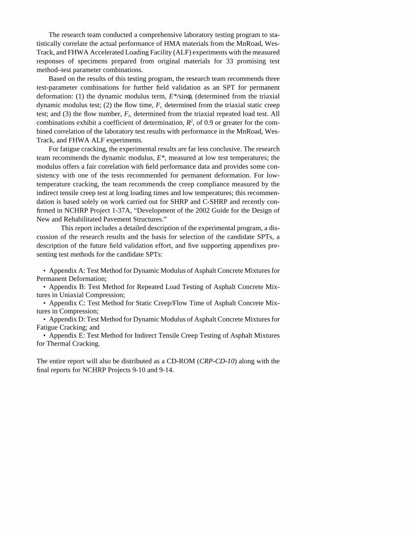
This report presents the findings of a research task to identify a simple test for con-firming key performance characteristics of Superpave volumetric mix designs. In thisinitial phase of the work, candidate tests for permanent deformation, fatigue cracking,and low-temperature cracking were identified and recommended for field validation inthe next phase of work. The report will be of particular interest to materials engineersin state highway agencies, as well as to materials suppliers and paving contractor per-sonnel responsible for design and production of hot mix asphalt.
The Superpave volumetric mix design procedure (AASHTO MP2 and PP28)developed in the Asphalt Research Program (1987–1993) of the Strategic HighwayResearch Program (SHRP) does not include a simple, mechanical “proof” test analo-gous to the Marshall stability and flow tests or the Hveem stabilometer method. Instead,the original Superpave method relied on strict conformance to the material specifica-tions and volumetric mix criteria to ensure satisfactory performance of mix designsintended for low-traffic-volume situations (defined as no more than 106 equivalent sin-gle axle loads [ESALs] applied over the service life of the pavement). For higher traf-ficked projects, the original SHRP Superpave mix analysis procedures1 required acheck for tertiary creep behavior with the repeated shear at constant stress ratio test(AASHTO TP7) and a rigorous evaluation of the mix design’s potential for permanentdeformation, fatigue cracking, and low-temperature cracking using several other com-plex test methods in AASHTO TP7 and TP9.
User experience with the Superpave mix design and analysis method, combinedwith the long-standing problems associated with the original SHRP Superpave perfor-mance models supporting what was then termed “Level 2 and 3” analyses, demon-strated the need for such simple performance tests (SPTs). In 1996, work sponsored byFHWA (Contract DTFH61-95-C-00100) began at the University of Maryland at Col-lege Park (UMCP) to identify and validate SPTs for permanent deformation, fatiguecracking, and low-temperature cracking to complement and support the Superpave vol-umetric mix design method. In 1999, this effort was transferred to Task C of NCHRPProject 9-19, “Superpave Support and Performance Models Management,” with themajor portion of the task conducted by a research team headed by UMCP subcontrac-tor Arizona State University (ASU).
The research team was directed to evaluate as potential SPTs only existing testmethods measuring hot mix asphalt (HMA) response characteristics. The principalevaluation criteria were (1) accuracy (i.e., good correlation of the HMA-response char-acteristic to actual field performance); (2) reliability (i.e., a minimum number of falsenegatives and positives); (3) ease of use; and (4) reasonable equipment cost.
1 The Superpave Mix Design Manual for New Construction and Overlays, Report SHRP-A-407, Strategic Highway ResearchProgram, National Research Council, Washington DC (1994).
The research team conducted a comprehensive laboratory testing program to sta-tistically correlate the actual performance of HMA materials from the MnRoad, Wes-Track, and FHWA Accelerated Loading Facility (ALF) experiments with the measuredresponses of specimens prepared from original materials for 33 promising testmethod–test parameter combinations.
Based on the results of this testing program, the research team recommends threetest-parameter combinations for further field validation as an SPT for permanentdeformation: (1) the dynamic modulus term, E*/sinφ, (determined from the triaxialdynamic modulus test; (2) the flow time, Ft, determined from the triaxial static creeptest; and (3) the flow number, Fn, determined from the triaxial repeated load test. Allcombinations exhibit a coefficient of determination, R2, of 0.9 or greater for the com-bined correlation of the laboratory test results with performance in the MnRoad, Wes-Track, and FHWA ALF experiments.
For fatigue cracking, the experimental results are far less conclusive. The researchteam recommends the dynamic modulus, E*, measured at low test temperatures; themodulus offers a fair correlation with field performance data and provides some con-sistency with one of the tests recommended for permanent deformation. For low-temperature cracking, the team recommends the creep compliance measured by theindirect tensile creep test at long loading times and low temperatures; this recommen-dation is based solely on work carried out for SHRP and C-SHRP and recently con-firmed in NCHRP Project 1-37A, “Development of the 2002 Guide for the Design ofNew and Rehabilitated Pavement Structures.”
This report includes a detailed description of the experimental program, a dis-cussion of the research results and the basis for selection of the candidate SPTs, adescription of the future field validation effort, and five supporting appendixes pre-senting test methods for the candidate SPTs:
• Appendix A: Test Method for Dynamic Modulus of Asphalt Concrete Mixtures forPermanent Deformation;
• Appendix B: Test Method for Repeated Load Testing of Asphalt Concrete Mix-tures in Uniaxial Compression;
• Appendix C: Test Method for Static Creep/Flow Time of Asphalt Concrete Mix-tures in Compression;
• Appendix D: Test Method for Dynamic Modulus of Asphalt Concrete Mixtures forFatigue Cracking; and
• Appendix E: Test Method for Indirect Tensile Creep Testing of Asphalt Mixturesfor Thermal Cracking.
The entire report will also be distributed as a CD-ROM (CRP-CD-10) along with thefinal reports for NCHRP Projects 9-10 and 9-14.
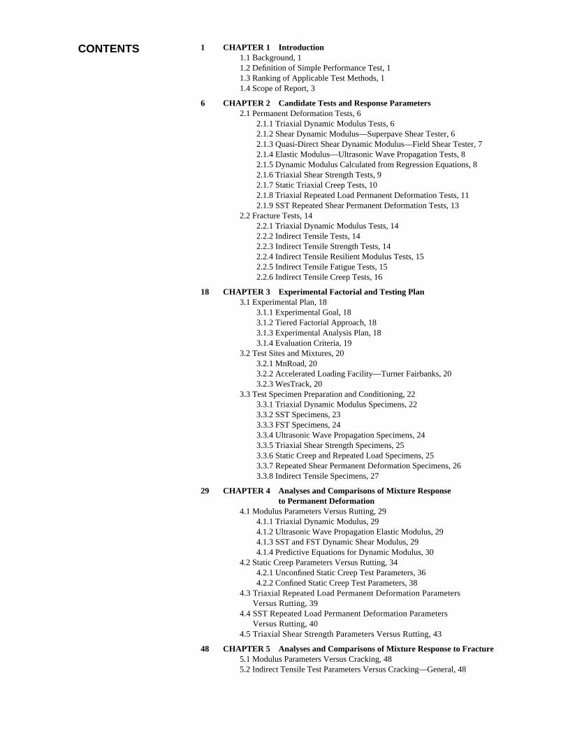
CONTENTS 1 CHAPTER 1 Introduction1.1 Background, 11.2 Definition of Simple Performance Test, 11.3 Ranking of Applicable Test Methods, 11.4 Scope of Report, 3
6 CHAPTER 2 Candidate Tests and Response Parameters2.1 Permanent Deformation Tests, 6
2.1.1 Triaxial Dynamic Modulus Tests, 62.1.2 Shear Dynamic Modulus—Superpave Shear Tester, 62.1.3 Quasi-Direct Shear Dynamic Modulus—Field Shear Tester, 72.1.4 Elastic Modulus—Ultrasonic Wave Propagation Tests, 82.1.5 Dynamic Modulus Calculated from Regression Equations, 82.1.6 Triaxial Shear Strength Tests, 92.1.7 Static Triaxial Creep Tests, 102.1.8 Triaxial Repeated Load Permanent Deformation Tests, 112.1.9 SST Repeated Shear Permanent Deformation Tests, 13
2.2 Fracture Tests, 142.2.1 Triaxial Dynamic Modulus Tests, 142.2.2 Indirect Tensile Tests, 142.2.3 Indirect Tensile Strength Tests, 142.2.4 Indirect Tensile Resilient Modulus Tests, 152.2.5 Indirect Tensile Fatigue Tests, 152.2.6 Indirect Tensile Creep Tests, 16
18 CHAPTER 3 Experimental Factorial and Testing Plan3.1 Experimental Plan, 18
3.1.1 Experimental Goal, 183.1.2 Tiered Factorial Approach, 183.1.3 Experimental Analysis Plan, 183.1.4 Evaluation Criteria, 19
3.2 Test Sites and Mixtures, 203.2.1 MnRoad, 203.2.2 Accelerated Loading Facility—Turner Fairbanks, 203.2.3 WesTrack, 20
3.3 Test Specimen Preparation and Conditioning, 223.3.1 Triaxial Dynamic Modulus Specimens, 223.3.2 SST Specimens, 233.3.3 FST Specimens, 243.3.4 Ultrasonic Wave Propagation Specimens, 243.3.5 Triaxial Shear Strength Specimens, 253.3.6 Static Creep and Repeated Load Specimens, 253.3.7 Repeated Shear Permanent Deformation Specimens, 263.3.8 Indirect Tensile Specimens, 27
29 CHAPTER 4 Analyses and Comparisons of Mixture Response to Permanent Deformation
4.1 Modulus Parameters Versus Rutting, 294.1.1 Triaxial Dynamic Modulus, 294.1.2 Ultrasonic Wave Propagation Elastic Modulus, 294.1.3 SST and FST Dynamic Shear Modulus, 294.1.4 Predictive Equations for Dynamic Modulus, 30
4.2 Static Creep Parameters Versus Rutting, 344.2.1 Unconfined Static Creep Test Parameters, 364.2.2 Confined Static Creep Test Parameters, 38
4.3 Triaxial Repeated Load Permanent Deformation Parameters Versus Rutting, 39
4.4 SST Repeated Load Permanent Deformation Parameters Versus Rutting, 40
4.5 Triaxial Shear Strength Parameters Versus Rutting, 43
48 CHAPTER 5 Analyses and Comparisons of Mixture Response to Fracture5.1 Modulus Parameters Versus Cracking, 485.2 Indirect Tensile Test Parameters Versus Cracking—General, 48
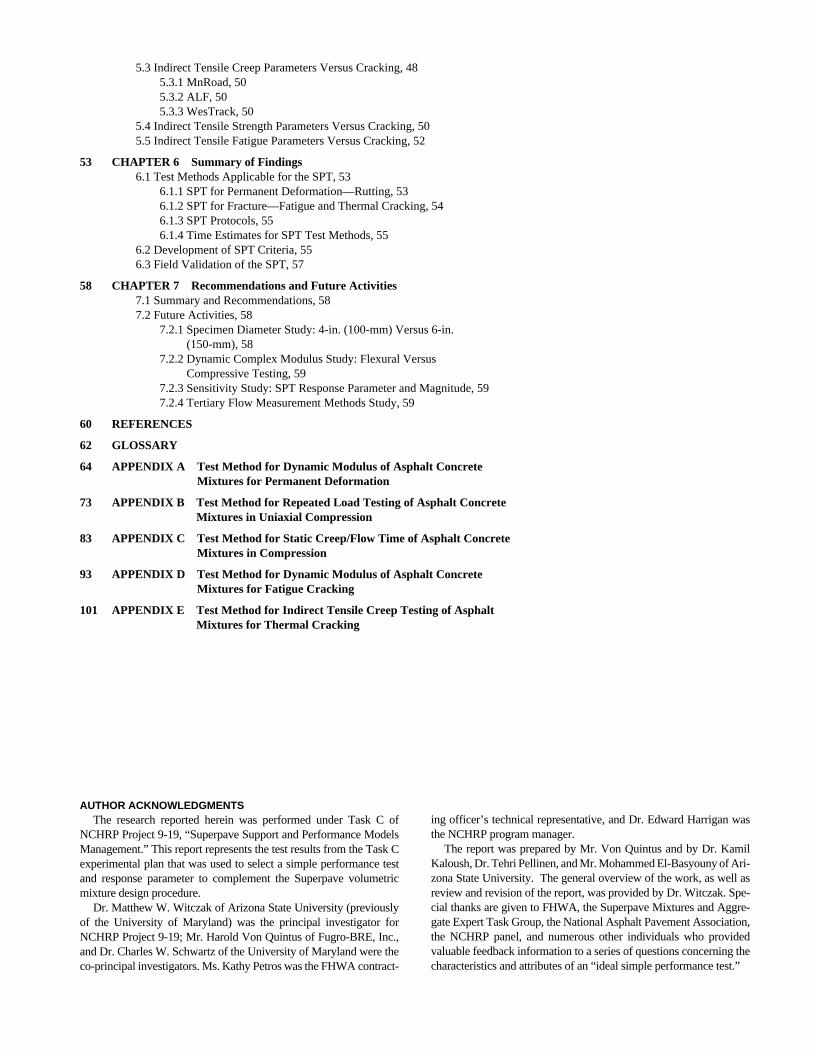
5.3 Indirect Tensile Creep Parameters Versus Cracking, 485.3.1 MnRoad, 505.3.2 ALF, 505.3.3 WesTrack, 50
5.4 Indirect Tensile Strength Parameters Versus Cracking, 505.5 Indirect Tensile Fatigue Parameters Versus Cracking, 52
53 CHAPTER 6 Summary of Findings 6.1 Test Methods Applicable for the SPT, 53
6.1.1 SPT for Permanent Deformation—Rutting, 536.1.2 SPT for Fracture—Fatigue and Thermal Cracking, 546.1.3 SPT Protocols, 556.1.4 Time Estimates for SPT Test Methods, 55
6.2 Development of SPT Criteria, 556.3 Field Validation of the SPT, 57
58 CHAPTER 7 Recommendations and Future Activities7.1 Summary and Recommendations, 587.2 Future Activities, 58
7.2.1 Specimen Diameter Study: 4-in. (100-mm) Versus 6-in.(150-mm), 58
7.2.2 Dynamic Complex Modulus Study: Flexural Versus Compressive Testing, 59
7.2.3 Sensitivity Study: SPT Response Parameter and Magnitude, 597.2.4 Tertiary Flow Measurement Methods Study, 59
60 REFERENCES
62 GLOSSARY
64 APPENDIX A Test Method for Dynamic Modulus of Asphalt Concrete Mixtures for Permanent Deformation
73 APPENDIX B Test Method for Repeated Load Testing of Asphalt ConcreteMixtures in Uniaxial Compression
83 APPENDIX C Test Method for Static Creep/Flow Time of Asphalt ConcreteMixtures in Compression
93 APPENDIX D Test Method for Dynamic Modulus of Asphalt Concrete Mixtures for Fatigue Cracking
101 APPENDIX E Test Method for Indirect Tensile Creep Testing of Asphalt Mixtures for Thermal Cracking
AUTHOR ACKNOWLEDGMENTSThe research reported herein was performed under Task C of
NCHRP Project 9-19, “Superpave Support and Performance ModelsManagement.” This report represents the test results from the Task Cexperimental plan that was used to select a simple performance testand response parameter to complement the Superpave volumetricmixture design procedure.
Dr. Matthew W. Witczak of Arizona State University (previouslyof the University of Maryland) was the principal investigator forNCHRP Project 9-19; Mr. Harold Von Quintus of Fugro-BRE, Inc.,and Dr. Charles W. Schwartz of the University of Maryland were theco-principal investigators. Ms. Kathy Petros was the FHWA contract-
ing officer’s technical representative, and Dr. Edward Harrigan wasthe NCHRP program manager.
The report was prepared by Mr. Von Quintus and by Dr. KamilKaloush, Dr. Tehri Pellinen, and Mr. Mohammed El-Basyouny of Ari-zona State University. The general overview of the work, as well asreview and revision of the report, was provided by Dr. Witczak. Spe-cial thanks are given to FHWA, the Superpave Mixtures and Aggre-gate Expert Task Group, the National Asphalt Pavement Association,the NCHRP panel, and numerous other individuals who providedvaluable feedback information to a series of questions concerning thecharacteristics and attributes of an “ideal simple performance test.”
1
CHAPTER 1
INTRODUCTION
1.1 BACKGROUND
The Superpave® mix design and analysis method was devel-oped more than a decade ago under the Strategic HighwayResearch Program (SHRP) (1). Many agencies in NorthAmerica have adopted different parts of that method, includ-ing the performance-grade (PG) binder specification and thevolumetric mixture design method.
The Superpave design method for hot mix asphalt (HMA)mixtures consists of three phases: (1) materials selection forthe asphalt binder and aggregate, (2) aggregate blending, and(3) volumetric analysis on specimens compacted using theSuperpave gyratory compactor (SGC) (2). However, otherthan a final check for tertiary flow, there is no generalstrength or “push–pull” test to complement the volumetricmixture design method as there is for the more traditionalMarshall and Hveem mixture design methods.
Results from WesTrack, NCHRP Project 9-7 (“Field Pro-cedures and Equipment to Implement SHRP Asphalt Speci-fications”), and other experimental construction projectshave raised the question of whether the Superpave volumet-ric mix design method alone is sufficient to ensure reliablemixture performance over a wide range of traffic and cli-matic conditions. Industry has expressed the need for asimple “push–pull” type of test to complement the Super-pave volumetric mix design method, especially for use ondesign–build or warranty projects.
In response to this need, FHWA committed funding in1996 to identify and evaluate a simplified test method.FHWA referred to this test as a “simple strength test” thatshould provide reliable information on the probable perfor-mance of the HMA design during the volumetric mixturedesign process using the SGC. The focus of the test was tomeasure a fundamental engineering property that can belinked back to the advanced material characterization meth-ods needed for detailed distress-prediction models. Thismeasurement would enable the use of a simple performancemodel in the development of criteria for HMA mixturedesign. It was envisioned that this simple strength or per-formance test would play a key role in the quality controland acceptance of HMA mixtures.
As a commitment to this effort, FHWA authorized theUniversity of Maryland Superpave Models Team (under
Phase II of FHWA Contract No. DTFH61-95-C-00100) todevelop all necessary test protocols, criteria, and guidelinesfor the simple performance test (SPT) to support the Super-pave volumetric mix design procedure. NCHRP Project 9-19(“Superpave Support and Performance Models Management”)continues that commitment.
1.2 DEFINITION OF SIMPLE PERFORMANCE TEST
The definition for the SPT, as used in this report, is asfollows:
A test method(s) that accurately and reliably measures amixture response characteristic or parameter that is highlycorrelated to the occurrence of pavement distress (e.g., crack-ing and rutting) over a diverse range of traffic and climaticconditions.
Given this definition, it is not necessary for the SPT to pre-dict the entire distress or performance history of the HMAmixture, but the test results must allow a determination of amixture’s ability to resist fracture and permanent deforma-tion under defined conditions.
1.3 RANKING OF APPLICABLE TESTMETHODS
As stated above, a consensus has been building amongmaterials and construction engineers, as well as among con-sultants and researchers, that an SPT should be included as afinal stage in the Superpave volumetric mix design method.That final stage is a diagnostic evaluation—the measurementand determination of properties related to performance—ofthe HMA mixture. The test methods that accurately and pre-cisely measure those properties and that are highly correlatedto pavement distress should be considered as candidates formore detailed laboratory studies.
Many tests have been proposed for use as an SPT, includ-ing dynamic modulus, repeated shear at constant height, shear
dynamic modulus, creep compliance, and other test methods.Under Phase II of the FHWA contract with the Universityof Maryland, the Superpave Models Team evaluated a vari-ety of possible tests that would be applicable to the defini-tion of an SPT.
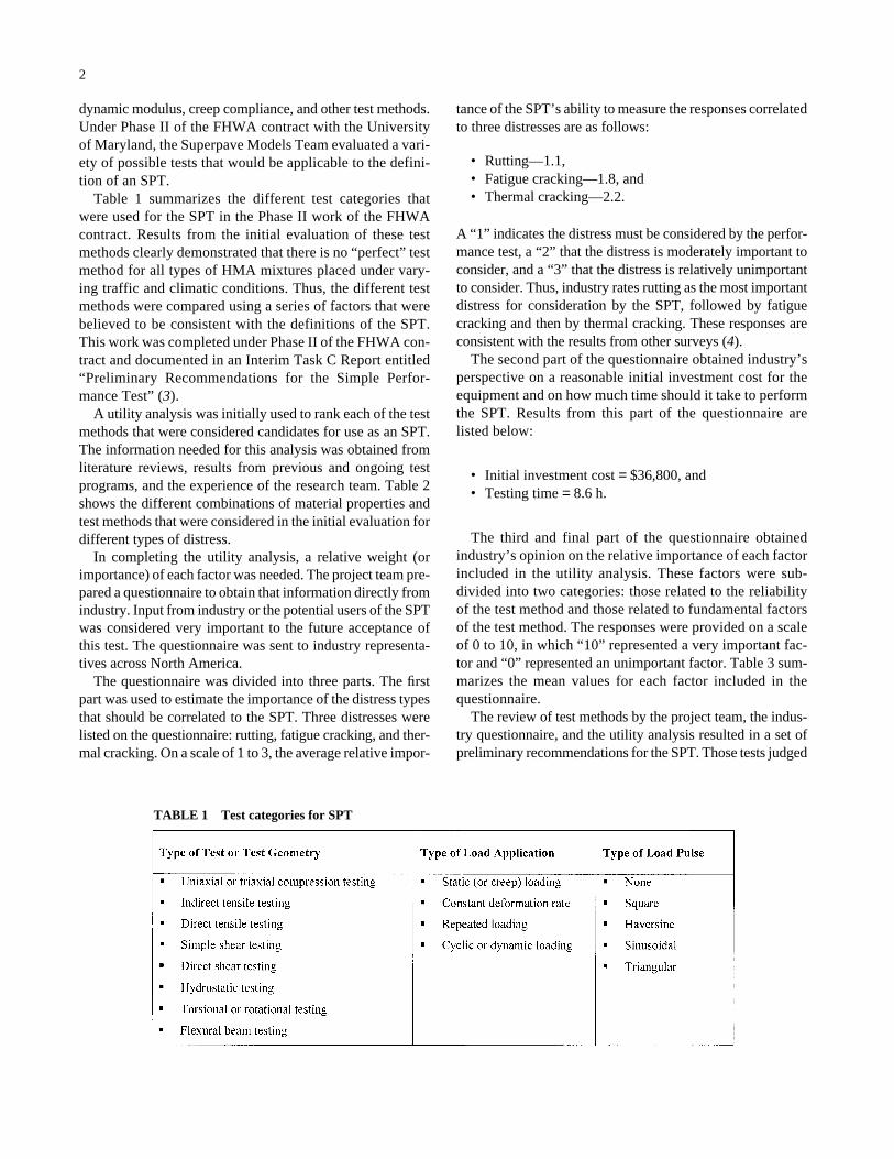
Table 1 summarizes the different test categories thatwere used for the SPT in the Phase II work of the FHWAcontract. Results from the initial evaluation of these testmethods clearly demonstrated that there is no “perfect” testmethod for all types of HMA mixtures placed under vary-ing traffic and climatic conditions. Thus, the different testmethods were compared using a series of factors that werebelieved to be consistent with the definitions of the SPT.This work was completed under Phase II of the FHWA con-tract and documented in an Interim Task C Report entitled“Preliminary Recommendations for the Simple Perfor-mance Test” (3).
A utility analysis was initially used to rank each of the testmethods that were considered candidates for use as an SPT.The information needed for this analysis was obtained fromliterature reviews, results from previous and ongoing testprograms, and the experience of the research team. Table 2shows the different combinations of material properties andtest methods that were considered in the initial evaluation fordifferent types of distress.
In completing the utility analysis, a relative weight (orimportance) of each factor was needed. The project team pre-pared a questionnaire to obtain that information directly fromindustry. Input from industry or the potential users of the SPTwas considered very important to the future acceptance ofthis test. The questionnaire was sent to industry representa-tives across North America.
The questionnaire was divided into three parts. The firstpart was used to estimate the importance of the distress typesthat should be correlated to the SPT. Three distresses werelisted on the questionnaire: rutting, fatigue cracking, and ther-mal cracking. On a scale of 1 to 3, the average relative impor-
2
tance of the SPT’s ability to measure the responses correlatedto three distresses are as follows:
• Rutting—1.1,• Fatigue cracking—1.8, and • Thermal cracking—2.2.
A “1” indicates the distress must be considered by the perfor-mance test, a “2” that the distress is moderately important toconsider, and a “3” that the distress is relatively unimportantto consider. Thus, industry rates rutting as the most importantdistress for consideration by the SPT, followed by fatiguecracking and then by thermal cracking. These responses areconsistent with the results from other surveys (4).
The second part of the questionnaire obtained industry’sperspective on a reasonable initial investment cost for theequipment and on how much time should it take to performthe SPT. Results from this part of the questionnaire arelisted below:
• Initial investment cost = $36,800, and • Testing time = 8.6 h.
The third and final part of the questionnaire obtainedindustry’s opinion on the relative importance of each factorincluded in the utility analysis. These factors were sub-divided into two categories: those related to the reliabilityof the test method and those related to fundamental factorsof the test method. The responses were provided on a scaleof 0 to 10, in which “10” represented a very important fac-tor and “0” represented an unimportant factor. Table 3 sum-marizes the mean values for each factor included in thequestionnaire.
The review of test methods by the project team, the indus-try questionnaire, and the utility analysis resulted in a set ofpreliminary recommendations for the SPT. Those tests judged
TABLE 1 Test categories for SPT
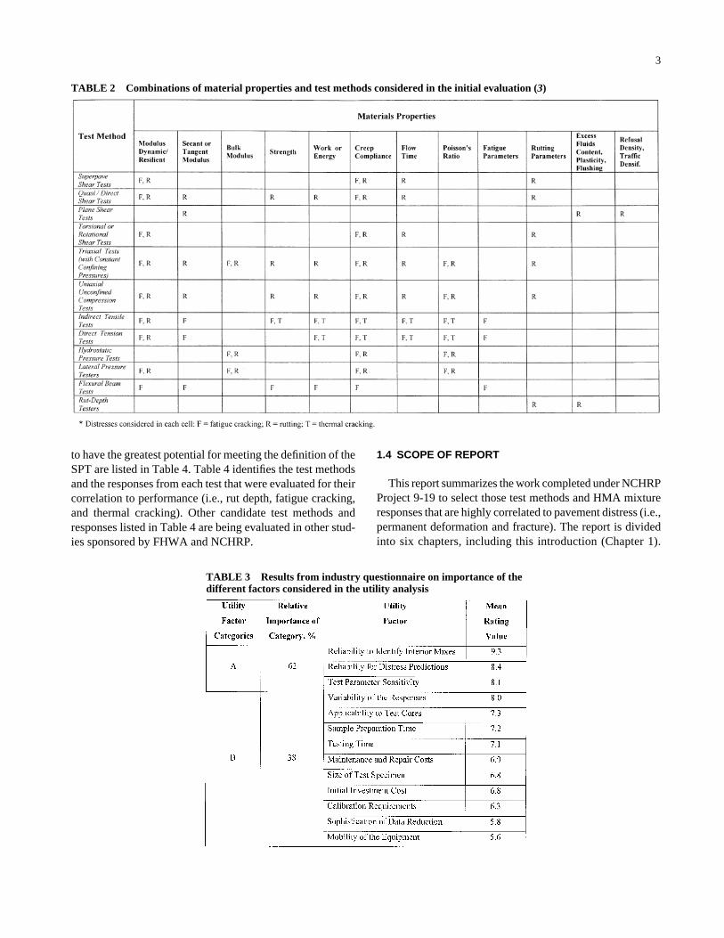
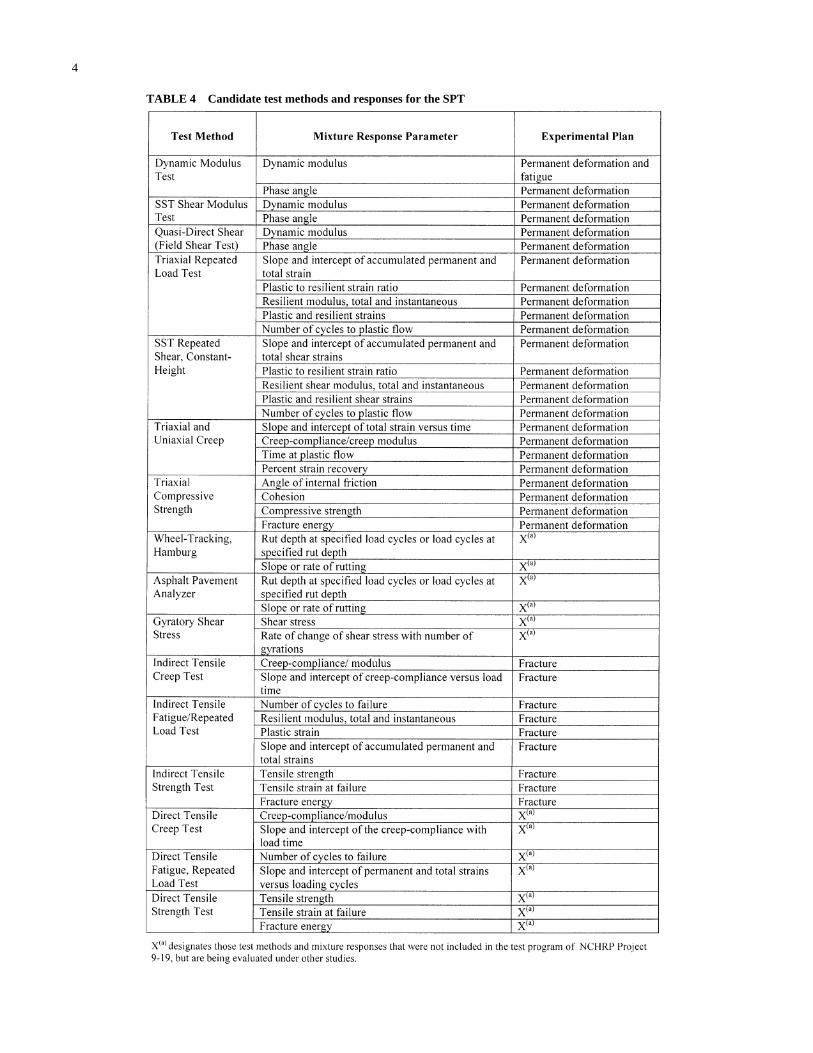
to have the greatest potential for meeting the definition of theSPT are listed in Table 4. Table 4 identifies the test methodsand the responses from each test that were evaluated for theircorrelation to performance (i.e., rut depth, fatigue cracking,and thermal cracking). Other candidate test methods andresponses listed in Table 4 are being evaluated in other stud-ies sponsored by FHWA and NCHRP.
3
1.4 SCOPE OF REPORT
This report summarizes the work completed under NCHRPProject 9-19 to select those test methods and HMA mixtureresponses that are highly correlated to pavement distress (i.e.,permanent deformation and fracture). The report is dividedinto six chapters, including this introduction (Chapter 1).
TABLE 2 Combinations of material properties and test methods considered in the initial evaluation (3)
TABLE 3 Results from industry questionnaire on importance of thedifferent factors considered in the utility analysis
4
TABLE 4 Candidate test methods and responses for the SPT

5
Chapter 2 provides a discussion of the candidate test meth-ods and mixture responses included in the test program.Chapter 3 presents the experimental factorial and details ofthe testing procedure for each test method. Chapters 4 and 5compare the mixture responses with permanent deformationand fracture (both fatigue and thermal cracking), respectively.
Chapter 6 summarizes the results and test methods recom-mended for the SPT and presents a framework for futuredevelopment of the specification criteria for the SPT and arecommended field validation experiment. The test protocolsrecommended for further field validation as SPTs are pro-vided in appendixes to the report.

6
CHAPTER 2
CANDIDATE TESTS AND RESPONSE PARAMETERS
Table 4 listed the test methods and mixture response para-meters that were ranked as the “best” candidates for the SPTfor permanent deformation and fracture distresses. This chap-ter describes the test methods and mixture response param-eters evaluated in NCHRP Project 9-19. Details of the lab-oratory test program are given in Chapter 3.
2.1 PERMANENT DEFORMATION TESTS
2.1.1 Triaxial Dynamic Modulus Tests
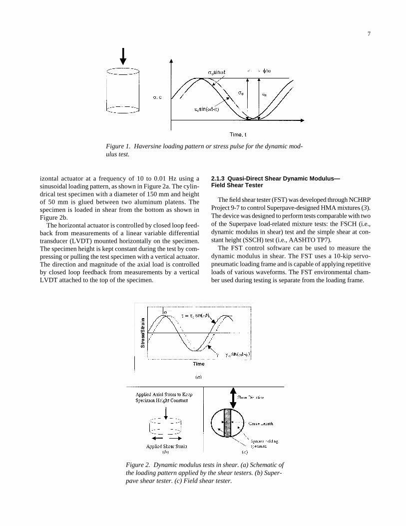
The dynamic modulus test is the oldest and best docu-mented of the triaxial compression tests. It was standardizedin 1979 as ASTM D3497, “Standard Test Method forDynamic Modulus of Asphalt Concrete Mixtures.” The testconsists of applying a uniaxial sinusoidal (i.e., haversine)compressive stress to an unconfined or confined HMA cylin-drical test specimen, as shown in Figure 1.
The stress-to-strain relationship under a continuous sinu-soidal loading for linear viscoelastic materials is defined bya complex number called the “complex modulus” (E*). Theabsolute value of the complex modulus, |E*|, is defined as thedynamic modulus. The dynamic modulus is mathematicallydefined as the maximum (i.e., peak) dynamic stress (σo)divided by the peak recoverable axial strain (εo):
(1)
The real and imaginary portions of the complex modulus(E*) can be written as
E* = E′ + iE″ (2)
E′ is generally referred to as the storage or elastic modu-lus component of the complex modulus; E″ is referred to asthe loss or viscous modulus. The phase angle, φ, is the angleby which εo lags behind σo. It is an indicator of the viscousproperties of the material being evaluated. Mathematically,this is expressed as
E* = |E*| cos φ + i |E*| sin φ (3)
E* o
o= σ
ε
(4)
where
ti = time lag between a cycle of stress and strain (s);tp = time for a stress cycle (s); andi = imaginary number.
For a pure elastic material, φ =0, and the complex modulus(E*) is equal to the absolute value, or dynamic modulus. Forpure viscous materials, φ =90°.
2.1.2 Shear Dynamic Modulus—SuperpaveShear Tester
The shear frequency sweep or shear dynamic modulus test(i.e., AASHTO TP7, “Standard Test Method for Determin-ing the Permanent Deformation and Fatigue Cracking Char-acteristics of Hot Mix Asphalt [HMA] Using the SimpleShear Test [SST] Device”) conducted with the Superpaveshear tester (SST) was developed under SHRP to measuremixture properties that can be used to predict mixture per-formance. The shear dynamic modulus is defined analo-gously to the triaxial dynamic modulus as the absolute valueof the complex modulus in shear:
(5)
where
|G*| =shear dynamic modulus,τ0 = peak shear stress amplitude, andγ0 = peak shear strain amplitude.
With these results, both the elastic and viscous behaviorcan be determined through calculation of the shear storagemodulus (G′) and loss modulus (G″ ), analogous to the dis-cussion for the dynamic modulus test.
The frequency sweep at constant height (FSCH) test is astrain-controlled test with the maximum shear strain lim-ited to 0.0001 mm/mm. The shear strain is applied by a hor-
G* = τγ
0
0
φ = ×tt
i
p( )360
7
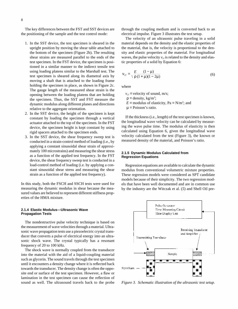
izontal actuator at a frequency of 10 to 0.01 Hz using asinusoidal loading pattern, as shown in Figure 2a. The cylin-drical test specimen with a diameter of 150 mm and heightof 50 mm is glued between two aluminum platens. Thespecimen is loaded in shear from the bottom as shown inFigure 2b.
The horizontal actuator is controlled by closed loop feed-back from measurements of a linear variable differentialtransducer (LVDT) mounted horizontally on the specimen.The specimen height is kept constant during the test by com-pressing or pulling the test specimen with a vertical actuator.The direction and magnitude of the axial load is controlledby closed loop feedback from measurements by a verticalLVDT attached to the top of the specimen.
2.1.3 Quasi-Direct Shear Dynamic Modulus—Field Shear Tester
The field shear tester (FST) was developed through NCHRPProject 9-7 to control Superpave-designed HMA mixtures (3).The device was designed to perform tests comparable with twoof the Superpave load-related mixture tests: the FSCH (i.e.,dynamic modulus in shear) test and the simple shear at con-stant height (SSCH) test (i.e., AASHTO TP7).
The FST control software can be used to measure thedynamic modulus in shear. The FST uses a 10-kip servo-pneumatic loading frame and is capable of applying repetitiveloads of various waveforms. The FST environmental cham-ber used during testing is separate from the loading frame.
Figure 1. Haversine loading pattern or stress pulse for the dynamic mod-ulus test.
Figure 2. Dynamic modulus tests in shear. (a) Schematic ofthe loading pattern applied by the shear testers. (b) Super-pave shear tester. (c) Field shear tester.
8
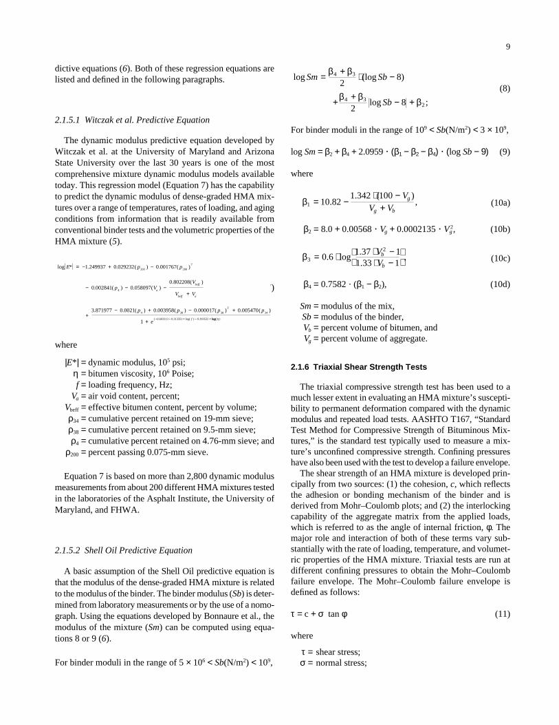
through the coupling medium and is converted back to anelectrical impulse. Figure 3 illustrates the test setup.
The velocity of an ultrasonic pulse traveling in a solidmaterial depends on the density and the elastic properties ofthe material, that is, the velocity is proportional to the den-sity and elastic properties of the material. For longitudinalwaves, the pulse velocity vcl is related to the density and elas-tic properties of a solid by Equation 6:
(6)
where
vcl = velocity of sound, m/s;ρ = density, kg/m3;E = modulus of elasticity, Pa = N/m2; andµ = Poisson’s ratio.
If the thickness (i.e., length) of the test specimen is known,the longitudinal wave velocity can be calculated by measur-ing the wave pulse time. The modulus of elasticity is thencalculated using Equation 6, given the longitudinal wavevelocity calculated from the test (Figure 3), the known ormeasured density of the material, and Poisson’s ratio.
2.1.5 Dynamic Modulus Calculated fromRegression Equations
Regression equations are available to calculate the dynamicmodulus from conventional volumetric mixture properties.These regression models were considered as SPT candidatemodels because of their simplicity. The two regression mod-els that have been well documented and are in common useby the industry are the Witczak et al. (5) and Shell Oil pre-
νρ
µµ µcl
E= −+ −
( )( )( )
11 1 2
The key differences between the FST and SST devices arethe positioning of the sample and the test control mode:
1. In the SST device, the test specimen is sheared in theupright position by moving the shear table attached tothe bottom of the specimen (Figure 2b). The resultingshear strains are measured parallel to the ends of thetest specimen. In the FST device, the specimen is posi-tioned in a similar manner to the indirect tensile testusing loading platens similar to the Marshall test. Thetest specimen is sheared along its diametral axis bymoving a shaft that is attached to the loading frameholding the specimen in place, as shown in Figure 2c.The gauge length of the measured shear strain is theopening between the loading platens that are holdingthe specimen. Thus, the SST and FST measure thedynamic modulus along different planes and directionsrelative to the aggregate orientation.
2. In the SST device, the height of the specimen is keptconstant by loading the specimen through a verticalactuator attached to the top of the specimen. In the FSTdevice, the specimen height is kept constant by usingrigid spacers attached to the specimen ends.
3. In the SST device, the shear frequency sweep test isconducted in a strain-control method of loading (i.e., byapplying a constant sinusoidal shear strain of approxi-mately 100 microstrains) and measuring the shear stressas a function of the applied test frequency. In the FSTdevice, the shear frequency sweep test is conducted in aload-control method of loading (i.e. by applying a con-stant sinusoidal shear stress and measuring the shearstrain as a function of the applied test frequency).
In this study, both the FSCH and SSCH tests were used formeasuring the dynamic modulus in shear because the mea-sured values are believed to represent different stiffness prop-erties of the HMA mixture.
2.1.4 Elastic Modulus—Ultrasonic WavePropagation Tests
The nondestructive pulse velocity technique is based onthe measurement of wave velocities through a material. Ultra-sonic wave propagation tests use a piezoelectric crystal trans-ducer that converts a pulse of electrical energy into an ultra-sonic shock wave. The crystal typically has a resonantfrequency of 20 to 100 kHz.
The shock wave is normally coupled from the transducerinto the material with the aid of a liquid-coupling materialsuch as glycerin. The sound travels through the test specimenuntil it encounters a density change where it is reflected backtowards the transducer. The density change is often the oppo-site end or surface of the test specimen. However, a flaw orlamination in the test specimen can cause the reflection ofsound as well. The ultrasound travels back to the probe Figure 3. Schematic illustration of the ultrasonic test setup.
dictive equations (6). Both of these regression equations arelisted and defined in the following paragraphs.
2.1.5.1 Witczak et al. Predictive Equation
The dynamic modulus predictive equation developed byWitczak et al. at the University of Maryland and ArizonaState University over the last 30 years is one of the mostcomprehensive mixture dynamic modulus models availabletoday. This regression model (Equation 7) has the capabilityto predict the dynamic modulus of dense-graded HMA mix-tures over a range of temperatures, rates of loading, and agingconditions from information that is readily available fromconventional binder tests and the volumetric properties of theHMA mixture (5).
(7)
where
|E*| =dynamic modulus, 105 psi;η = bitumen viscosity, 106 Poise;f = loading frequency, Hz;
Va = air void content, percent;Vbeff = effective bitumen content, percent by volume;ρ34 = cumulative percent retained on 19-mm sieve;ρ38 = cumulative percent retained on 9.5-mm sieve;ρ4 = cumulative percent retained on 4.76-mm sieve; and
ρ200 = percent passing 0.075-mm sieve.
Equation 7 is based on more than 2,800 dynamic modulusmeasurements from about 200 different HMA mixtures testedin the laboratories of the Asphalt Institute, the University ofMaryland, and FHWA.
2.1.5.2 Shell Oil Predictive Equation
A basic assumption of the Shell Oil predictive equation isthat the modulus of the dense-graded HMA mixture is relatedto the modulus of the binder. The binder modulus (Sb) is deter-mined from laboratory measurements or by the use of a nomo-graph. Using the equations developed by Bonnaure et al., themodulus of the mixture (Sm) can be computed using equa-tions 8 or 9 (6).
For binder moduli in the range of 5 × 10⁶ < Sb(N/m2) < 109,
log * . . ( ) . ( )
. ( ) . ( ). ( )
. . ( ) . ( ) . ( ) . ( )
( . . log( ) .
E p p
p VV
V V
p p p p
e
a
beff
beff a
f
= − + −
− − −+
+− + − +
+ − − × − ×
1 249937 0 029232 0 001767
0 002841 0 0580970 802208
3 871977 0 0021 0 003958 0 000017 0 005470
1
200 200
2
4
4 38 38
2
34
0 603313 0 313351 0 393532 log(log( )η
9
(8)
For binder moduli in the range of 109 < Sb(N/m2) < 3 × 10⁹,
log Sm = β2 + β4 + 2.0959 � (β1 − β2 − β4) � (log Sb − 9) (9)
where
(10a)
β2 = 8.0 + 0.00568 � Vg + 0.0002135 � Vg2, (10b)
(10c)
β4 = 0.7582 � (β1 − β2), (10d)
Sm = modulus of the mix,Sb = modulus of the binder,Vb = percent volume of bitumen, and Vg = percent volume of aggregate.
2.1.6 Triaxial Shear Strength Tests
The triaxial compressive strength test has been used to amuch lesser extent in evaluating an HMA mixture’s suscepti-bility to permanent deformation compared with the dynamicmodulus and repeated load tests. AASHTO T167, “StandardTest Method for Compressive Strength of Bituminous Mix-tures,” is the standard test typically used to measure a mix-ture’s unconfined compressive strength. Confining pressureshave also been used with the test to develop a failure envelope.
The shear strength of an HMA mixture is developed prin-cipally from two sources: (1) the cohesion, c, which reflectsthe adhesion or bonding mechanism of the binder and isderived from Mohr–Coulomb plots; and (2) the interlockingcapability of the aggregate matrix from the applied loads,which is referred to as the angle of internal friction, φ. Themajor role and interaction of both of these terms vary sub-stantially with the rate of loading, temperature, and volumet-ric properties of the HMA mixture. Triaxial tests are run atdifferent confining pressures to obtain the Mohr–Coulombfailure envelope. The Mohr–Coulomb failure envelope isdefined as follows:
τ = c + σ tan φ (11)
where
τ = shear stress;σ = normal stress;
β3
2
0 61 37 11 33 1
= ⋅ ⋅ −⋅ −
. log
..
,VV
b
b
β1 10 821 342 100
= −⋅ −
+.
. ( ),
VV V
g
g b
log (log )
log ;
Sm Sb
Sb
= + ⋅ −
+ + − +
β β
β β β
4 3
4 32
28
28
c = intercept parameter, cohesion; andφ = slope of the failure envelope or the angle of internal
friction.
Typical c-values for dense-graded HMA mixtures are inthe range of 5 to 35 psi; typical φ-values range between 35°and 48°. Triaxial tests usually require three or more levels ofconfinement to accurately determine the failure envelope.
An alternative to the Mohr–Coulomb failure envelope isthe Drucker–Prager failure envelope, which is defined by anintercept parameter, k, and slope γ1/2 (7). The Drucker–Pragerfailure envelope represents the combination of failurestresses expressed in terms of the first invariant stress tensor,I1, and the second invariant deviatoric stress tensor, J 2
1/2, bythe following equation:
(12)
where
J21/2 = (1/√3) (σ1 − σ3), and I1 = σ1 + 2σ3.
2.1.7 Static Triaxial Creep Tests
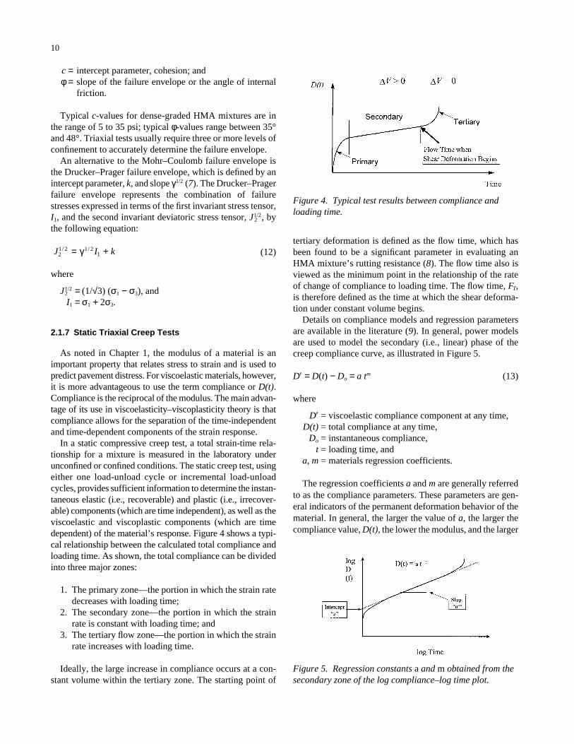
As noted in Chapter 1, the modulus of a material is animportant property that relates stress to strain and is used topredict pavement distress. For viscoelastic materials, however,it is more advantageous to use the term compliance or D(t).Compliance is the reciprocal of the modulus. The main advan-tage of its use in viscoelasticity–viscoplasticity theory is thatcompliance allows for the separation of the time-independentand time-dependent components of the strain response.
In a static compressive creep test, a total strain-time rela-tionship for a mixture is measured in the laboratory underunconfined or confined conditions. The static creep test, usingeither one load-unload cycle or incremental load-unloadcycles, provides sufficient information to determine the instan-taneous elastic (i.e., recoverable) and plastic (i.e., irrecover-able) components (which are time independent), as well as theviscoelastic and viscoplastic components (which are timedependent) of the material’s response. Figure 4 shows a typi-cal relationship between the calculated total compliance andloading time. As shown, the total compliance can be dividedinto three major zones:
1. The primary zone—the portion in which the strain ratedecreases with loading time;
2. The secondary zone—the portion in which the strainrate is constant with loading time; and
3. The tertiary flow zone—the portion in which the strainrate increases with loading time.
Ideally, the large increase in compliance occurs at a con-stant volume within the tertiary zone. The starting point of
J I k21 2 1 2
1/ /= +γ
10
tertiary deformation is defined as the flow time, which hasbeen found to be a significant parameter in evaluating anHMA mixture’s rutting resistance (8). The flow time also isviewed as the minimum point in the relationship of the rateof change of compliance to loading time. The flow time, FT,is therefore defined as the time at which the shear deforma-tion under constant volume begins.
Details on compliance models and regression parametersare available in the literature (9). In general, power modelsare used to model the secondary (i.e., linear) phase of thecreep compliance curve, as illustrated in Figure 5.
D′ = D(t) − Do = a tm (13)
where
D′ = viscoelastic compliance component at any time,D(t) = total compliance at any time,
Do = instantaneous compliance, t = loading time, and
a, m = materials regression coefficients.
The regression coefficients a and m are generally referredto as the compliance parameters. These parameters are gen-eral indicators of the permanent deformation behavior of thematerial. In general, the larger the value of a, the larger thecompliance value, D(t), the lower the modulus, and the larger
Figure 4. Typical test results between compliance andloading time.
Figure 5. Regression constants a and m obtained from thesecondary zone of the log compliance–log time plot.
the permanent deformation. For a constant a-value, anincrease in the slope parameter m means higher permanentdeformation.
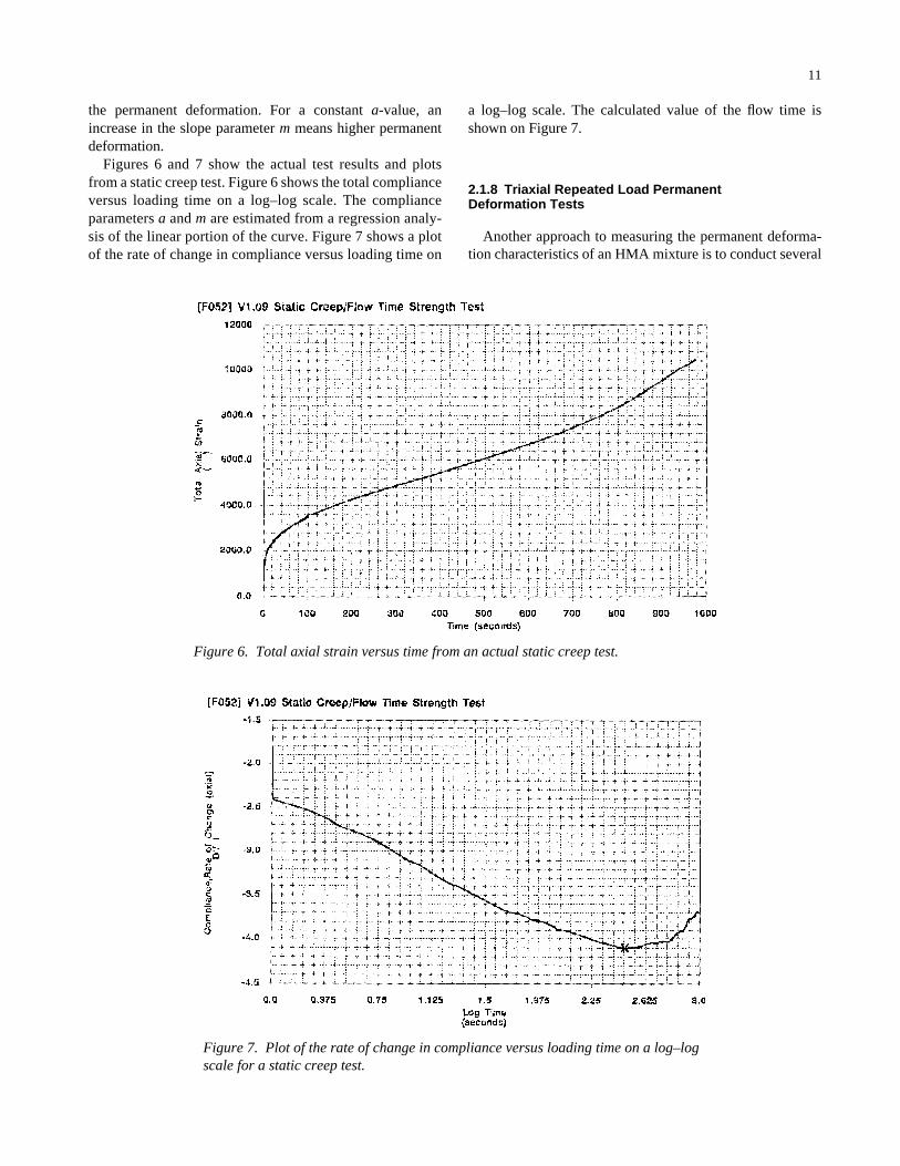
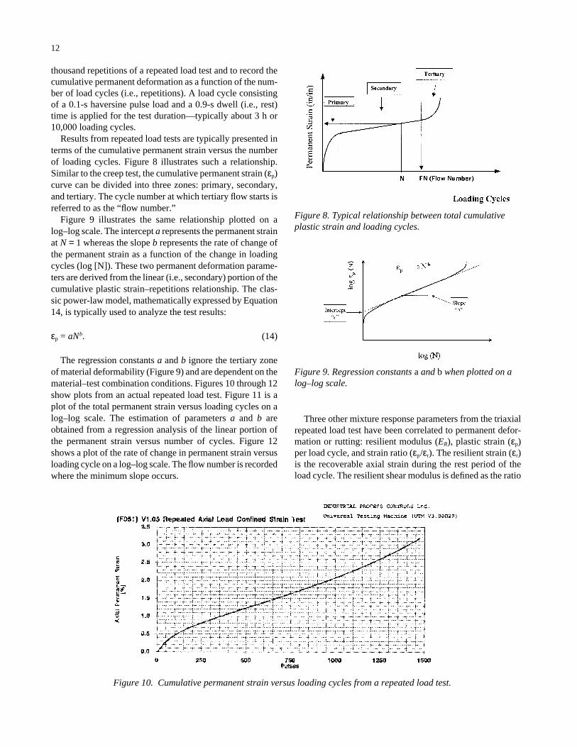
Figures 6 and 7 show the actual test results and plotsfrom a static creep test. Figure 6 shows the total complianceversus loading time on a log–log scale. The complianceparameters a and m are estimated from a regression analy-sis of the linear portion of the curve. Figure 7 shows a plotof the rate of change in compliance versus loading time on
11
a log–log scale. The calculated value of the flow time isshown on Figure 7.
2.1.8 Triaxial Repeated Load PermanentDeformation Tests
Another approach to measuring the permanent deforma-tion characteristics of an HMA mixture is to conduct several
Figure 6. Total axial strain versus time from an actual static creep test.
Figure 7. Plot of the rate of change in compliance versus loading time on a log–logscale for a static creep test.
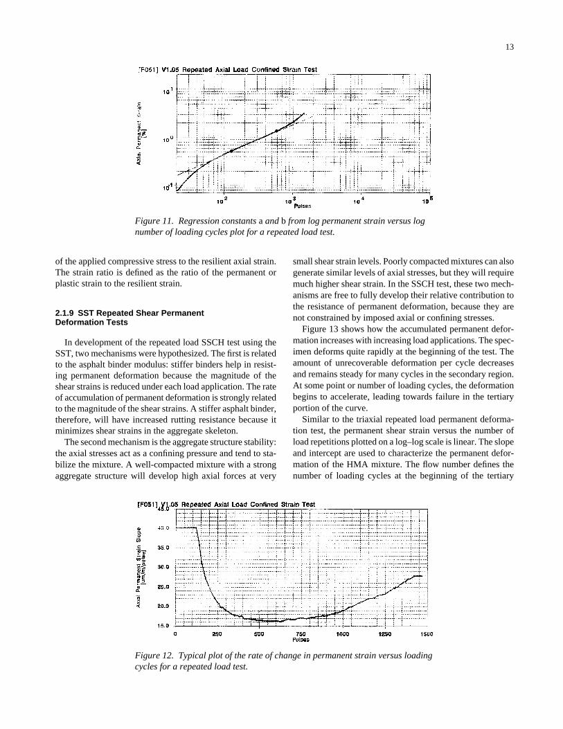
thousand repetitions of a repeated load test and to record thecumulative permanent deformation as a function of the num-ber of load cycles (i.e., repetitions). A load cycle consistingof a 0.1-s haversine pulse load and a 0.9-s dwell (i.e., rest)time is applied for the test duration—typically about 3 h or10,000 loading cycles.
Results from repeated load tests are typically presented interms of the cumulative permanent strain versus the numberof loading cycles. Figure 8 illustrates such a relationship.Similar to the creep test, the cumulative permanent strain (εp)curve can be divided into three zones: primary, secondary,and tertiary. The cycle number at which tertiary flow starts isreferred to as the “flow number.”
Figure 9 illustrates the same relationship plotted on alog–log scale. The intercept a represents the permanent strainat N = 1 whereas the slope b represents the rate of change ofthe permanent strain as a function of the change in loadingcycles (log [N]). These two permanent deformation parame-ters are derived from the linear (i.e., secondary) portion of thecumulative plastic strain–repetitions relationship. The clas-sic power-law model, mathematically expressed by Equation14, is typically used to analyze the test results:
εp = aNb. (14)
The regression constants a and b ignore the tertiary zoneof material deformability (Figure 9) and are dependent on thematerial–test combination conditions. Figures 10 through 12show plots from an actual repeated load test. Figure 11 is aplot of the total permanent strain versus loading cycles on alog–log scale. The estimation of parameters a and b areobtained from a regression analysis of the linear portion ofthe permanent strain versus number of cycles. Figure 12shows a plot of the rate of change in permanent strain versusloading cycle on a log–log scale. The flow number is recordedwhere the minimum slope occurs.
12
Three other mixture response parameters from the triaxialrepeated load test have been correlated to permanent defor-mation or rutting: resilient modulus (ER), plastic strain (εp)per load cycle, and strain ratio (εp/εr). The resilient strain (εr)is the recoverable axial strain during the rest period of theload cycle. The resilient shear modulus is defined as the ratio
Figure 8. Typical relationship between total cumulativeplastic strain and loading cycles.
Figure 9. Regression constants a and b when plotted on alog–log scale.
Figure 10. Cumulative permanent strain versus loading cycles from a repeated load test.
of the applied compressive stress to the resilient axial strain.The strain ratio is defined as the ratio of the permanent orplastic strain to the resilient strain.
2.1.9 SST Repeated Shear PermanentDeformation Tests
In development of the repeated load SSCH test using theSST, two mechanisms were hypothesized. The first is relatedto the asphalt binder modulus: stiffer binders help in resist-ing permanent deformation because the magnitude of theshear strains is reduced under each load application. The rateof accumulation of permanent deformation is strongly relatedto the magnitude of the shear strains. A stiffer asphalt binder,therefore, will have increased rutting resistance because itminimizes shear strains in the aggregate skeleton.
The second mechanism is the aggregate structure stability:the axial stresses act as a confining pressure and tend to sta-bilize the mixture. A well-compacted mixture with a strongaggregate structure will develop high axial forces at very
13
small shear strain levels. Poorly compacted mixtures can alsogenerate similar levels of axial stresses, but they will requiremuch higher shear strain. In the SSCH test, these two mech-anisms are free to fully develop their relative contribution tothe resistance of permanent deformation, because they arenot constrained by imposed axial or confining stresses.
Figure 13 shows how the accumulated permanent defor-mation increases with increasing load applications. The spec-imen deforms quite rapidly at the beginning of the test. Theamount of unrecoverable deformation per cycle decreasesand remains steady for many cycles in the secondary region.At some point or number of loading cycles, the deformationbegins to accelerate, leading towards failure in the tertiaryportion of the curve.
Similar to the triaxial repeated load permanent deforma-tion test, the permanent shear strain versus the number ofload repetitions plotted on a log–log scale is linear. The slopeand intercept are used to characterize the permanent defor-mation of the HMA mixture. The flow number defines thenumber of loading cycles at the beginning of the tertiary
Figure 12. Typical plot of the rate of change in permanent strain versus loadingcycles for a repeated load test.
Figure 11. Regression constants a and b from log permanent strain versus lognumber of loading cycles plot for a repeated load test.
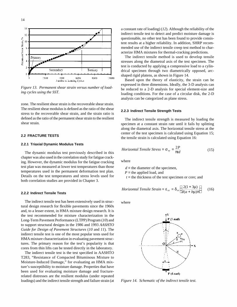
zone. The resilient shear strain is the recoverable shear strain.The resilient shear modulus is defined as the ratio of the shearstress to the recoverable shear strain, and the strain ratio isdefined as the ratio of the permanent shear strain to the resilientshear strain.
2.2 FRACTURE TESTS
2.2.1 Triaxial Dynamic Modulus Tests
The dynamic modulus test previously described in thischapter was also used in the correlation study for fatigue crack-ing. However, the dynamic modulus for the fatigue crackingtest plan was measured at lower test temperatures than thosetemperatures used in the permanent deformation test plan.Details on the test temperatures and stress levels used forboth correlation studies are provided in Chapter 3.
2.2.2 Indirect Tensile Tests
The indirect tensile test has been extensively used in struc-tural design research for flexible pavements since the 1960sand, to a lesser extent, in HMA mixture design research. It isthe test recommended for mixture characterization in theLong-Term Pavement Performance (LTPP) Program (10) andto support structural designs in the 1986 and 1993 AASHTOGuide for Design of Pavement Structures (10 and 11). Theindirect tensile test is one of the most popular tests used forHMA mixture characterization in evaluating pavement struc-tures. The primary reason for the test’s popularity is thatcores from thin lifts can be tested directly in the laboratory.
The indirect tensile test is the test specified in AASHTOT283, “Resistance of Compacted Bituminous Mixture toMoisture-Induced Damage,” for evaluating an HMA mix-ture’s susceptibility to moisture damage. Properties that havebeen used for evaluating moisture damage and fracture-related distresses are the resilient modulus (under repeatedloadings) and the indirect tensile strength and failure strain (at
14
a constant rate of loading) (12). Although the reliability of theindirect tensile test to detect and predict moisture damage isquestionable, no other test has been found to provide consis-tent results at a higher reliability. In addition, SHRP recom-mended use of the indirect tensile creep test method to char-acterize HMA mixtures for thermal-cracking predictions.
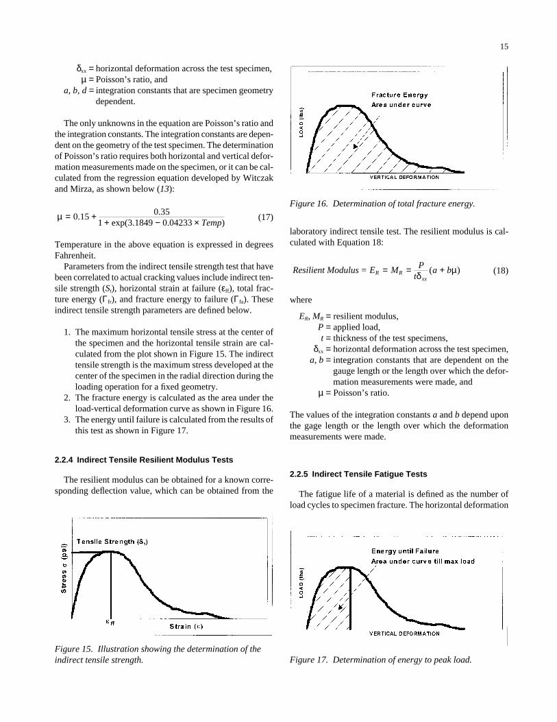
The indirect tensile method is used to develop tensilestresses along the diametral axis of the test specimen. Thetest is conducted by applying a compressive load to a cylin-drical specimen through two diametrically opposed, arc-shaped rigid platens, as shown in Figure 14.
Based upon the theory of elasticity, the strain can beexpressed in three dimensions. Ideally, the 3-D analysis canbe reduced to a 2-D analysis for special element-size andloading conditions. For the case of a circular disk, the 2-Danalysis can be categorized as plane stress.
2.2.3 Indirect Tensile Strength Tests
The indirect tensile strength is measured by loading thespecimen at a constant strain rate until it fails by splittingalong the diametral axis. The horizontal tensile stress at thecenter of the test specimen is calculated using Equation 15;the tensile strain is calculated using Equation 16:
(15)
where
d = the diameter of the specimen,P = the applied load, andt = the thickness of the test specimen or core; and
(16)
where
Horizontal Tensile Straind a bxx xx= = +
+
ε δ µ
µ π2 1 3( )( )
Horizontal Tensile Stress Ptdxy= =σ
π2
Figure 13. Permanent shear strain versus number of load-ing cycles using the SST.
Figure 14. Schematic of the indirect tensile test.
δxx = horizontal deformation across the test specimen,µ = Poisson’s ratio, and
a, b, d = integration constants that are specimen geometrydependent.
The only unknowns in the equation are Poisson’s ratio andthe integration constants. The integration constants are depen-dent on the geometry of the test specimen. The determinationof Poisson’s ratio requires both horizontal and vertical defor-mation measurements made on the specimen, or it can be cal-culated from the regression equation developed by Witczakand Mirza, as shown below (13):
(17)
Temperature in the above equation is expressed in degreesFahrenheit.
Parameters from the indirect tensile strength test that havebeen correlated to actual cracking values include indirect ten-sile strength (St), horizontal strain at failure (εff), total frac-ture energy (Γfr), and fracture energy to failure (Γfa). Theseindirect tensile strength parameters are defined below.
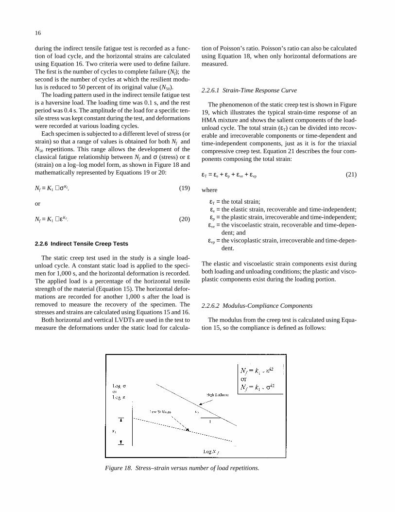
1. The maximum horizontal tensile stress at the center ofthe specimen and the horizontal tensile strain are cal-culated from the plot shown in Figure 15. The indirecttensile strength is the maximum stress developed at thecenter of the specimen in the radial direction during theloading operation for a fixed geometry.
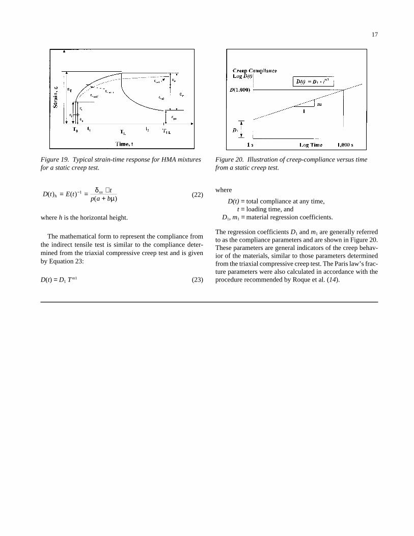
2. The fracture energy is calculated as the area under theload-vertical deformation curve as shown in Figure 16.
3. The energy until failure is calculated from the results ofthis test as shown in Figure 17.
2.2.4 Indirect Tensile Resilient Modulus Tests
The resilient modulus can be obtained for a known corre-sponding deflection value, which can be obtained from the
µ = ++ − ×
0 15 0 351 3 1849 0 04233
. .exp( . . )Temp
15
laboratory indirect tensile test. The resilient modulus is cal-culated with Equation 18:
(18)
where
ER, MR = resilient modulus,P = applied load,t = thickness of the test specimens,
δxx = horizontal deformation across the test specimen,a, b = integration constants that are dependent on the
gauge length or the length over which the defor-mation measurements were made, and
µ = Poisson’s ratio.
The values of the integration constants a and b depend uponthe gage length or the length over which the deformationmeasurements were made.
2.2.5 Indirect Tensile Fatigue Tests
The fatigue life of a material is defined as the number ofload cycles to specimen fracture. The horizontal deformation
Resilient Modulus E M Pt
a bR Rxx
= = = +δ
µ( )
Figure 15. Illustration showing the determination of theindirect tensile strength.
Figure 16. Determination of total fracture energy.
Figure 17. Determination of energy to peak load.
during the indirect tensile fatigue test is recorded as a func-tion of load cycle, and the horizontal strains are calculatedusing Equation 16. Two criteria were used to define failure.The first is the number of cycles to complete failure (Nf); thesecond is the number of cycles at which the resilient modu-lus is reduced to 50 percent of its original value (N50).
The loading pattern used in the indirect tensile fatigue testis a haversine load. The loading time was 0.1 s, and the restperiod was 0.4 s. The amplitude of the load for a specific ten-sile stress was kept constant during the test, and deformationswere recorded at various loading cycles.
Each specimen is subjected to a different level of stress (orstrain) so that a range of values is obtained for both Nf andN50 repetitions. This range allows the development of theclassical fatigue relationship between Nf and σ (stress) or ε(strain) on a log–log model form, as shown in Figure 18 andmathematically represented by Equations 19 or 20:
Nf = K1 ∗ σ K2, (19)
or
Nf = K1 ∗ ε K2. (20)
2.2.6 Indirect Tensile Creep Tests
The static creep test used in the study is a single load-unload cycle. A constant static load is applied to the speci-men for 1,000 s, and the horizontal deformation is recorded.The applied load is a percentage of the horizontal tensilestrength of the material (Equation 15). The horizontal defor-mations are recorded for another 1,000 s after the load isremoved to measure the recovery of the specimen. Thestresses and strains are calculated using Equations 15 and 16.
Both horizontal and vertical LVDTs are used in the test tomeasure the deformations under the static load for calcula-
16
tion of Poisson’s ratio. Poisson’s ratio can also be calculatedusing Equation 18, when only horizontal deformations aremeasured.
2.2.6.1 Strain-Time Response Curve
The phenomenon of the static creep test is shown in Figure19, which illustrates the typical strain-time response of anHMA mixture and shows the salient components of the load-unload cycle. The total strain (εT) can be divided into recov-erable and irrecoverable components or time-dependent andtime-independent components, just as it is for the triaxialcompressive creep test. Equation 21 describes the four com-ponents composing the total strain:
εT = εe + εp + εve + εvp (21)
where
εT = the total strain;εe = the elastic strain, recoverable and time-independent;εp = the plastic strain, irrecoverable and time-independent;εve = the viscoelastic strain, recoverable and time-depen-
dent; and εvp = the viscoplastic strain, irrecoverable and time-depen-
dent.
The elastic and viscoelastic strain components exist duringboth loading and unloading conditions; the plastic and visco-plastic components exist during the loading portion.
2.2.6.2 Modulus-Compliance Components
The modulus from the creep test is calculated using Equa-tion 15, so the compliance is defined as follows:
Figure 18. Stress–strain versus number of load repetitions.
(22)
where h is the horizontal height.
The mathematical form to represent the compliance fromthe indirect tensile test is similar to the compliance deter-mined from the triaxial compressive creep test and is givenby Equation 23:
D(t) = D1 Tm1 (23)
D t E tt
p a bhxx( ) ( )
( )= = ∗
+−1 δ
µ
17
where
D(t) = total compliance at any time,t = loading time, and
D1, m1 = material regression coefficients.
The regression coefficients D1 and m1 are generally referredto as the compliance parameters and are shown in Figure 20.These parameters are general indicators of the creep behav-ior of the materials, similar to those parameters determinedfrom the triaxial compressive creep test. The Paris law’s frac-ture parameters were also calculated in accordance with theprocedure recommended by Roque et al. (14).
Figure 19. Typical strain-time response for HMA mixturesfor a static creep test.
Figure 20. Illustration of creep-compliance versus timefrom a static creep test.
18
CHAPTER 3
EXPERIMENTAL FACTORIAL AND TESTING PLAN
3.1 EXPERIMENTAL PLAN
The experimental plan was designed to investigate sepa-rately both major distresses—deformability and fracture. Apractical, reliable HMA mix design method must be based ona set of compromising principles that balance the volumetriccomponents to optimize the mix’s flexibility to prevent frac-ture while maintaining adequate stiffness to resist deforma-tion. This balance was clearly recognized by the individualsresponding to the utility analysis questionnaire discussed inChapter 1.
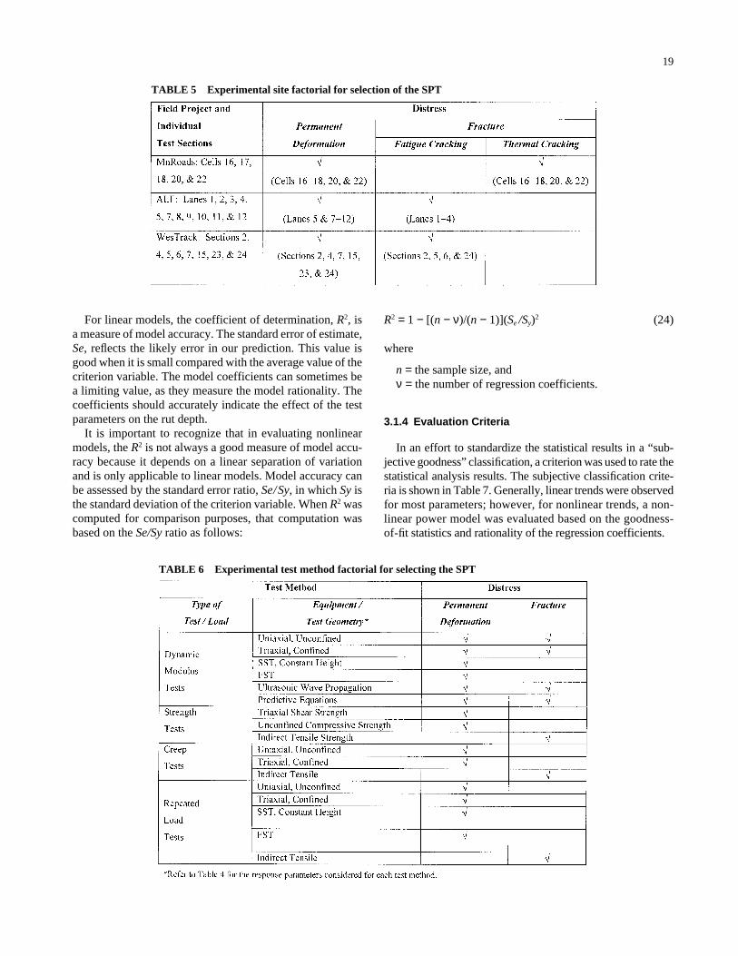
Although both major distress manifestations were pursuedin this work, it is important to recognize that rutting was ratedas the most significant HMA mixture problem in currentpractice. Thus, the experimental plan for selecting the SPTemploys the higher level of effort to quantify the deforma-bility of HMA mixtures. Table 5 shows the three test sitesand mixture distresses included in the experimental factorial.Each test site is discussed in this chapter.
3.1.1 Experimental Goal
The goal of the experimental plan was to use field projectswith a diverse range of distress magnitudes to select the testmethods and mixture response parameters that are most highlycorrelated to rutting and cracking. Table 6 shows the exper-imental factorial for the test methods and responses for eachdistress.
The HMA materials and mixtures were sampled fromthese projects to recompact test specimens with the SGC tothe volumetric properties reported during mixture placement.The measured responses from those test methods (Table 6)were compared with the observed distress at each project.The projects identified for use in this study were those hav-ing multiple test sections that are identical with the exceptionof the composition of the HMA mixture. Thus, the individ-ual goal of each field project was to allow for the relativecomparison of the measured response parameters to distresswithin that project.
3.1.2 Tiered Factorial Approach
The testing plan was to concentrate on those “mechanisticand fundamental” response parameters that could be linked
to the advanced material characterization tests, which alsoare being developed as a part of NCHRP Project 9-19. Thislinkage is one of the major requirements of the SPT.
The initial work completed under Phase II of the FHWAcontract resulted in a significant number of candidates for theSPT (Table 4). Rather than subjectively eliminating some ofthe candidate test methods, it was decided to actually evalu-ate as many of the candidate test protocols as possible in aphased laboratory study. As a consequence, the laboratoryexperimental factorial was divided into different projects.
A wide variety of test methods and responses were used inthe laboratory effort in the first part of the experimental plan.The HMA mixture responses were compared with each dis-tress on a project-by-project basis. Those test methods thatwere found to have inconsistent relationships or that resultedin poor correlations with the distress magnitude were removedfrom further consideration in the other projects. The test meth-ods and response parameters found to be highly correlatedwith the distress observations at a project then were evalu-ated in the other projects.
3.1.3 Experimental Analysis Plan
For the experiment design, it was hypothesized that the testmethods and responses ranked as the “best” candidates for theSPT could be used to identify HMA mixtures that are sus-ceptible to permanent deformation and fracture over a diverserange of materials, climates, pavement structures, and supportconditions. The experimental analysis plan was devised toquantify the correlation between mixture response and dis-tress on a project-by-project basis.
Statistical analyses were conducted to evaluate all measuredlaboratory responses on how they compared with observeddistress measurements. The analysis was completed for eachdistress by developing plots of the distress for each test sec-tion against the laboratory-measured test parameter. Trendsand regression models were statistically evaluated based onthe goodness-of-fit parameters: coefficient of determination,R2, standard error of estimate, Se, relative accuracy, Se/Sy, andassessment of the model rationality. Two types of regressionmodels were used in the comparisons, a linear and nonlinearmodel. The nonlinear model was based on the power law.
19
For linear models, the coefficient of determination, R2, isa measure of model accuracy. The standard error of estimate,Se, reflects the likely error in our prediction. This value isgood when it is small compared with the average value of thecriterion variable. The model coefficients can sometimes bea limiting value, as they measure the model rationality. Thecoefficients should accurately indicate the effect of the testparameters on the rut depth.
It is important to recognize that in evaluating nonlinearmodels, the R2 is not always a good measure of model accu-racy because it depends on a linear separation of variationand is only applicable to linear models. Model accuracy canbe assessed by the standard error ratio, Se/Sy, in which Sy isthe standard deviation of the criterion variable. When R2 wascomputed for comparison purposes, that computation wasbased on the Se/Sy ratio as follows:
R2 = 1 − [(n − ν)/(n − 1)](Se /Sy)2 (24)
where
n = the sample size, andν = the number of regression coefficients.
3.1.4 Evaluation Criteria
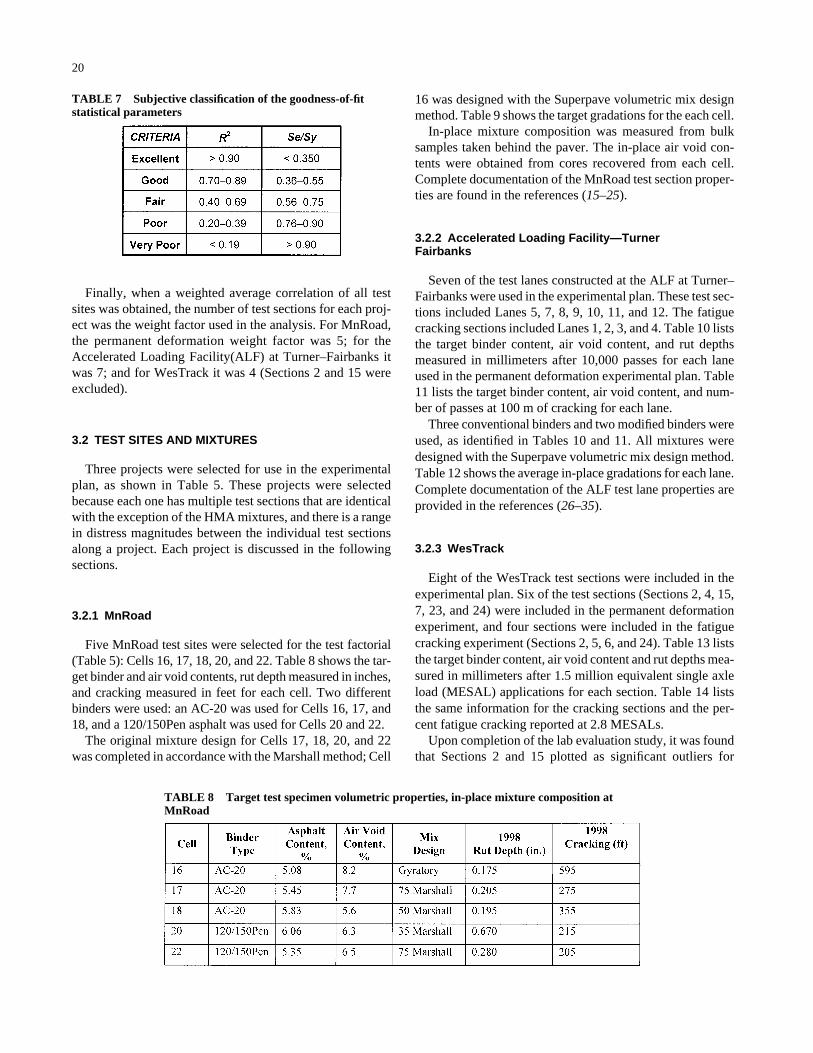
In an effort to standardize the statistical results in a “sub-jective goodness” classification, a criterion was used to rate thestatistical analysis results. The subjective classification crite-ria is shown in Table 7. Generally, linear trends were observedfor most parameters; however, for nonlinear trends, a non-linear power model was evaluated based on the goodness-of-fit statistics and rationality of the regression coefficients.
TABLE 5 Experimental site factorial for selection of the SPT
TABLE 6 Experimental test method factorial for selecting the SPT
20
16 was designed with the Superpave volumetric mix designmethod. Table 9 shows the target gradations for the each cell.
In-place mixture composition was measured from bulksamples taken behind the paver. The in-place air void con-tents were obtained from cores recovered from each cell.Complete documentation of the MnRoad test section proper-ties are found in the references (15–25).
3.2.2 Accelerated Loading Facility—TurnerFairbanks
Seven of the test lanes constructed at the ALF at Turner–Fairbanks were used in the experimental plan. These test sec-tions included Lanes 5, 7, 8, 9, 10, 11, and 12. The fatiguecracking sections included Lanes 1, 2, 3, and 4. Table 10 liststhe target binder content, air void content, and rut depthsmeasured in millimeters after 10,000 passes for each laneused in the permanent deformation experimental plan. Table11 lists the target binder content, air void content, and num-ber of passes at 100 m of cracking for each lane.
Three conventional binders and two modified binders wereused, as identified in Tables 10 and 11. All mixtures weredesigned with the Superpave volumetric mix design method.Table 12 shows the average in-place gradations for each lane.Complete documentation of the ALF test lane properties areprovided in the references (26–35).
3.2.3 WesTrack
Eight of the WesTrack test sections were included in theexperimental plan. Six of the test sections (Sections 2, 4, 15,7, 23, and 24) were included in the permanent deformationexperiment, and four sections were included in the fatiguecracking experiment (Sections 2, 5, 6, and 24). Table 13 liststhe target binder content, air void content and rut depths mea-sured in millimeters after 1.5 million equivalent single axleload (MESAL) applications for each section. Table 14 liststhe same information for the cracking sections and the per-cent fatigue cracking reported at 2.8 MESALs.
Upon completion of the lab evaluation study, it was foundthat Sections 2 and 15 plotted as significant outliers for
Finally, when a weighted average correlation of all testsites was obtained, the number of test sections for each proj-ect was the weight factor used in the analysis. For MnRoad,the permanent deformation weight factor was 5; for theAccelerated Loading Facility(ALF) at Turner–Fairbanks itwas 7; and for WesTrack it was 4 (Sections 2 and 15 wereexcluded).
3.2 TEST SITES AND MIXTURES
Three projects were selected for use in the experimentalplan, as shown in Table 5. These projects were selectedbecause each one has multiple test sections that are identicalwith the exception of the HMA mixtures, and there is a rangein distress magnitudes between the individual test sectionsalong a project. Each project is discussed in the followingsections.
3.2.1 MnRoad
Five MnRoad test sites were selected for the test factorial(Table 5): Cells 16, 17, 18, 20, and 22. Table 8 shows the tar-get binder and air void contents, rut depth measured in inches,and cracking measured in feet for each cell. Two differentbinders were used: an AC-20 was used for Cells 16, 17, and18, and a 120/150Pen asphalt was used for Cells 20 and 22.
The original mixture design for Cells 17, 18, 20, and 22was completed in accordance with the Marshall method; Cell
TABLE 7 Subjective classification of the goodness-of-fitstatistical parameters
TABLE 8 Target test specimen volumetric properties, in-place mixture composition atMnRoad
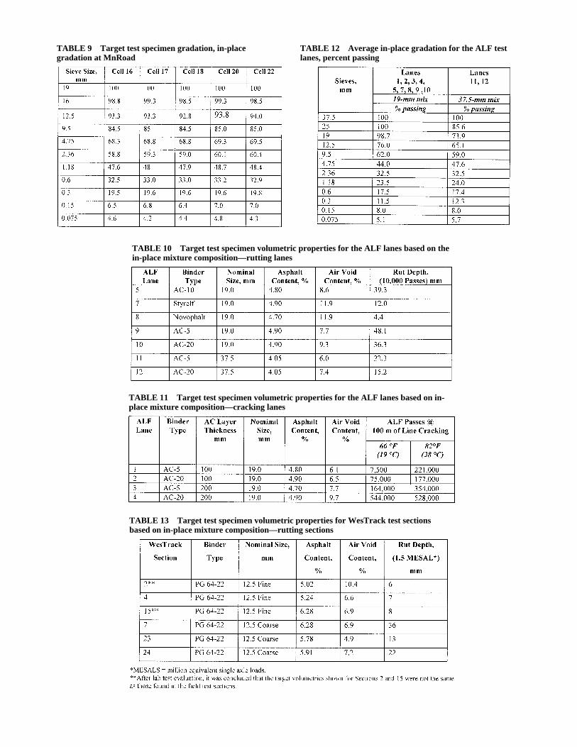
TABLE 9 Target test specimen gradation, in-placegradation at MnRoad
TABLE 10 Target test specimen volumetric properties for the ALF lanes based on thein-place mixture composition—rutting lanes
TABLE 11 Target test specimen volumetric properties for the ALF lanes based on in-place mixture composition—cracking lanes
TABLE 12 Average in-place gradation for the ALF testlanes, percent passing
TABLE 13 Target test specimen volumetric properties for WesTrack test sectionsbased on in-place mixture composition—rutting sections
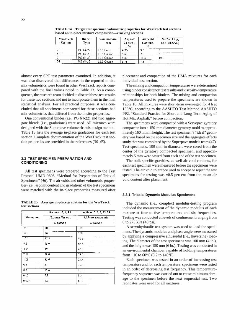
almost every SPT test parameter examined. In addition, itwas also discovered that differences in the reported in situmix volumetrics were found in other WesTrack reports com-pared with the final values noted in Table 13. As a conse-quence, the research team decided to discard these test resultsfor these two sections and not to incorporate them in the finalstatistical analysis. For all practical purposes, it was con-cluded that all specimens compacted for these sections hadmix volumetrics that differed from the in situ properties.
One conventional binder (i.e., PG 64-22) and two aggre-gate blends (i.e., gradations) were used. All mixtures weredesigned with the Superpave volumetric mix design method.Table 15 lists the average in-place gradations for each testsection. Complete documentation of the WesTrack test sec-tion properties are provided in the references (36–45).
3.3 TEST SPECIMEN PREPARATION ANDCONDITIONING
All test specimens were prepared according to the TestProtocol UMD 9808, “Method for Preparation of TriaxialSpecimens” (46). The air voids and other volumetric proper-ties (i.e., asphalt content and gradation) of the test specimenswere matched with the in-place properties measured after
22
placement and compaction of the HMA mixtures for eachindividual test section.
The mixing and compaction temperatures were determinedusing binder consistency test results and viscosity-temperaturerelationships for both binders. The mixing and compactiontemperatures used to prepare the specimens are shown inTable 16. All mixtures were short-term oven-aged for 4 h at135°C, according to the AASHTO Test Method AASHTOPP2, “Standard Practice for Short and Long Term Aging ofHot Mix Asphalt,” before compaction.
The specimens were compacted with a Servopac gyratorycompactor into a 150-mm diameter gyratory mold to approx-imately 160 mm in height. The test specimen’s “ideal” geom-etry was based on the specimen size and the aggregate effectsstudy that was completed by the Superpave models team (47).Test specimens, 100 mm in diameter, were cored from thecenter of the gyratory compacted specimen, and approxi-mately 5 mm were sawed from each end of the test specimen.
The bulk specific gravities, as well air void contents, foreach test specimen were measured before the specimens weretested. The air void tolerance used to accept or reject the testspecimens for testing was ±0.5 percent from the mean airvoid content after placement.
3.3.1 Triaxial Dynamic Modulus Specimens
The dynamic (i.e., complex) modulus-testing programincluded the measurement of the dynamic modulus of eachmixture at four to five temperatures and six frequencies.Testing was conducted at levels of confinement ranging from0 to 275 kPa (40 psi).
A servohydraulic test system was used to load the speci-mens. The dynamic modulus and phase angle were measuredby applying a compressive sinusoidal (i.e., haversine) load-ing. The diameter of the test specimens was 100 mm (4 in.),and the height was 150 mm (6 in.). Testing was conducted inan environmental chamber capable of holding temperaturesfrom −16 to 60°C (3.2 to 140°F).
Each specimen was tested in an order of increasing testtemperature and for each temperature; specimens were testedin an order of decreasing test frequency. This temperature-frequency sequence was carried out to cause minimum dam-age to the specimen before the next sequential test. Tworeplicates were used for all mixtures.
TABLE 14 Target test specimen volumetric properties for WesTrack test sectionsbased on in-place mixture composition—cracking sections
TABLE 15 Average in-place gradation for the WesTracktest sections
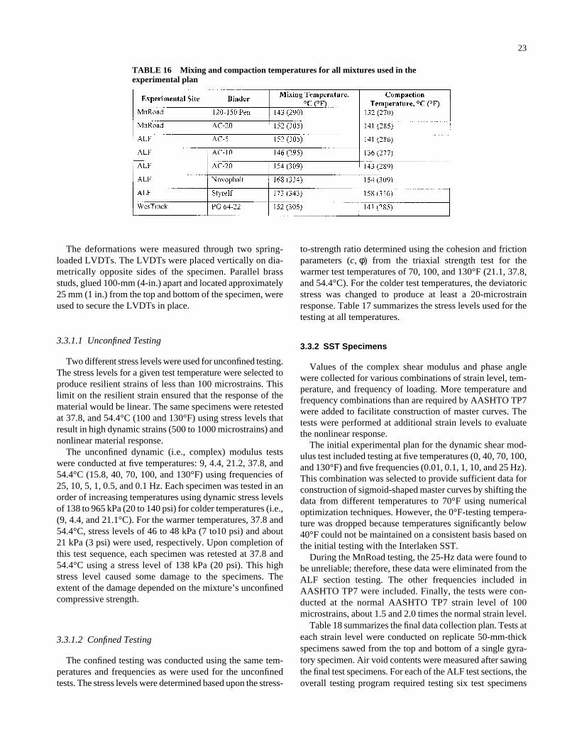
The deformations were measured through two spring-loaded LVDTs. The LVDTs were placed vertically on dia-metrically opposite sides of the specimen. Parallel brassstuds, glued 100-mm (4-in.) apart and located approximately25 mm (1 in.) from the top and bottom of the specimen, wereused to secure the LVDTs in place.
3.3.1.1 Unconfined Testing
Two different stress levels were used for unconfined testing.The stress levels for a given test temperature were selected toproduce resilient strains of less than 100 microstrains. Thislimit on the resilient strain ensured that the response of thematerial would be linear. The same specimens were retestedat 37.8, and 54.4°C (100 and 130°F) using stress levels thatresult in high dynamic strains (500 to 1000 microstrains) andnonlinear material response.
The unconfined dynamic (i.e., complex) modulus testswere conducted at five temperatures: 9, 4.4, 21.2, 37.8, and54.4°C (15.8, 40, 70, 100, and 130°F) using frequencies of25, 10, 5, 1, 0.5, and 0.1 Hz. Each specimen was tested in anorder of increasing temperatures using dynamic stress levelsof 138 to 965 kPa (20 to 140 psi) for colder temperatures (i.e.,(9, 4.4, and 21.1°C). For the warmer temperatures, 37.8 and54.4°C, stress levels of 46 to 48 kPa (7 to10 psi) and about21 kPa (3 psi) were used, respectively. Upon completion ofthis test sequence, each specimen was retested at 37.8 and54.4°C using a stress level of 138 kPa (20 psi). This highstress level caused some damage to the specimens. Theextent of the damage depended on the mixture’s unconfinedcompressive strength.
3.3.1.2 Confined Testing
The confined testing was conducted using the same tem-peratures and frequencies as were used for the unconfinedtests. The stress levels were determined based upon the stress-
23
to-strength ratio determined using the cohesion and frictionparameters (c, φ) from the triaxial strength test for thewarmer test temperatures of 70, 100, and 130°F (21.1, 37.8,and 54.4°C). For the colder test temperatures, the deviatoricstress was changed to produce at least a 20-microstrainresponse. Table 17 summarizes the stress levels used for thetesting at all temperatures.
3.3.2 SST Specimens
Values of the complex shear modulus and phase anglewere collected for various combinations of strain level, tem-perature, and frequency of loading. More temperature andfrequency combinations than are required by AASHTO TP7were added to facilitate construction of master curves. Thetests were performed at additional strain levels to evaluatethe nonlinear response.
The initial experimental plan for the dynamic shear mod-ulus test included testing at five temperatures (0, 40, 70, 100,and 130°F) and five frequencies (0.01, 0.1, 1, 10, and 25 Hz).This combination was selected to provide sufficient data forconstruction of sigmoid-shaped master curves by shifting thedata from different temperatures to 70°F using numericaloptimization techniques. However, the 0°F-testing tempera-ture was dropped because temperatures significantly below40°F could not be maintained on a consistent basis based onthe initial testing with the Interlaken SST.
During the MnRoad testing, the 25-Hz data were found tobe unreliable; therefore, these data were eliminated from theALF section testing. The other frequencies included inAASHTO TP7 were included. Finally, the tests were con-ducted at the normal AASHTO TP7 strain level of 100microstrains, about 1.5 and 2.0 times the normal strain level.
Table 18 summarizes the final data collection plan. Tests ateach strain level were conducted on replicate 50-mm-thickspecimens sawed from the top and bottom of a single gyra-tory specimen. Air void contents were measured after sawingthe final test specimens. For each of the ALF test sections, theoverall testing program required testing six test specimens
TABLE 16 Mixing and compaction temperatures for all mixtures used in theexperimental plan
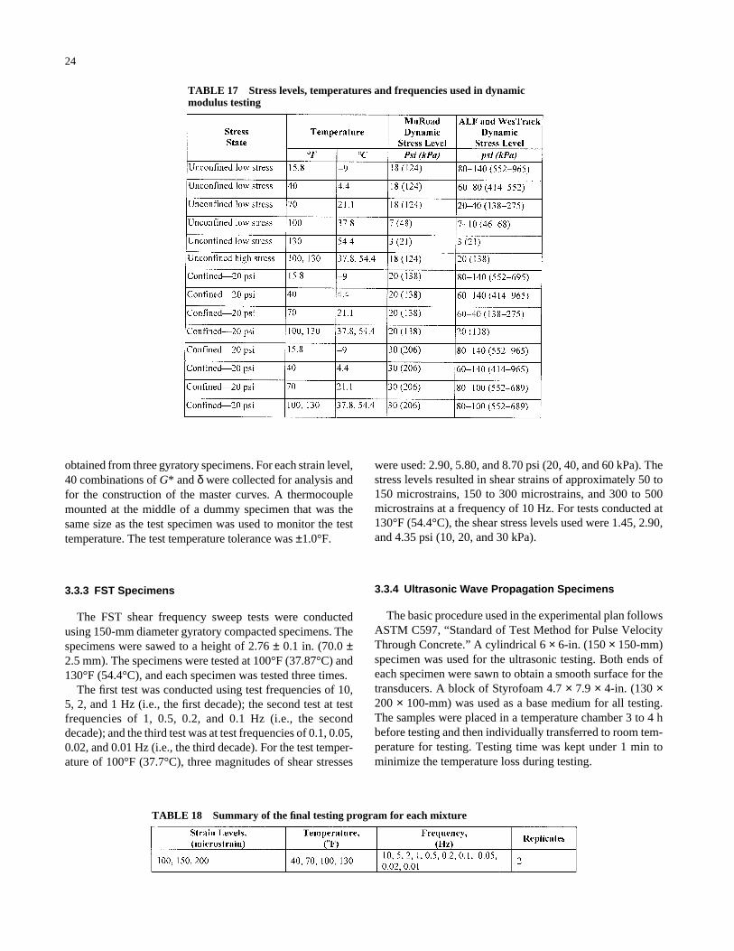
obtained from three gyratory specimens. For each strain level,40 combinations of G* and δ were collected for analysis andfor the construction of the master curves. A thermocouplemounted at the middle of a dummy specimen that was thesame size as the test specimen was used to monitor the testtemperature. The test temperature tolerance was ±1.0°F.
3.3.3 FST Specimens
The FST shear frequency sweep tests were conductedusing 150-mm diameter gyratory compacted specimens. Thespecimens were sawed to a height of 2.76 ± 0.1 in. (70.0 ±2.5 mm). The specimens were tested at 100°F (37.87°C) and130°F (54.4°C), and each specimen was tested three times.
The first test was conducted using test frequencies of 10,5, 2, and 1 Hz (i.e., the first decade); the second test at testfrequencies of 1, 0.5, 0.2, and 0.1 Hz (i.e., the seconddecade); and the third test was at test frequencies of 0.1, 0.05,0.02, and 0.01 Hz (i.e., the third decade). For the test temper-ature of 100°F (37.7°C), three magnitudes of shear stresses
24
were used: 2.90, 5.80, and 8.70 psi (20, 40, and 60 kPa). Thestress levels resulted in shear strains of approximately 50 to150 microstrains, 150 to 300 microstrains, and 300 to 500microstrains at a frequency of 10 Hz. For tests conducted at130°F (54.4°C), the shear stress levels used were 1.45, 2.90,and 4.35 psi (10, 20, and 30 kPa).
3.3.4 Ultrasonic Wave Propagation Specimens
The basic procedure used in the experimental plan followsASTM C597, “Standard of Test Method for Pulse VelocityThrough Concrete.” A cylindrical 6 × 6-in. (150 × 150-mm)specimen was used for the ultrasonic testing. Both ends ofeach specimen were sawn to obtain a smooth surface for thetransducers. A block of Styrofoam 4.7 × 7.9 × 4-in. (130 ×200 × 100-mm) was used as a base medium for all testing.The samples were placed in a temperature chamber 3 to 4 hbefore testing and then individually transferred to room tem-perature for testing. Testing time was kept under 1 min tominimize the temperature loss during testing.
TABLE 18 Summary of the final testing program for each mixture
TABLE 17 Stress levels, temperatures and frequencies used in dynamicmodulus testing
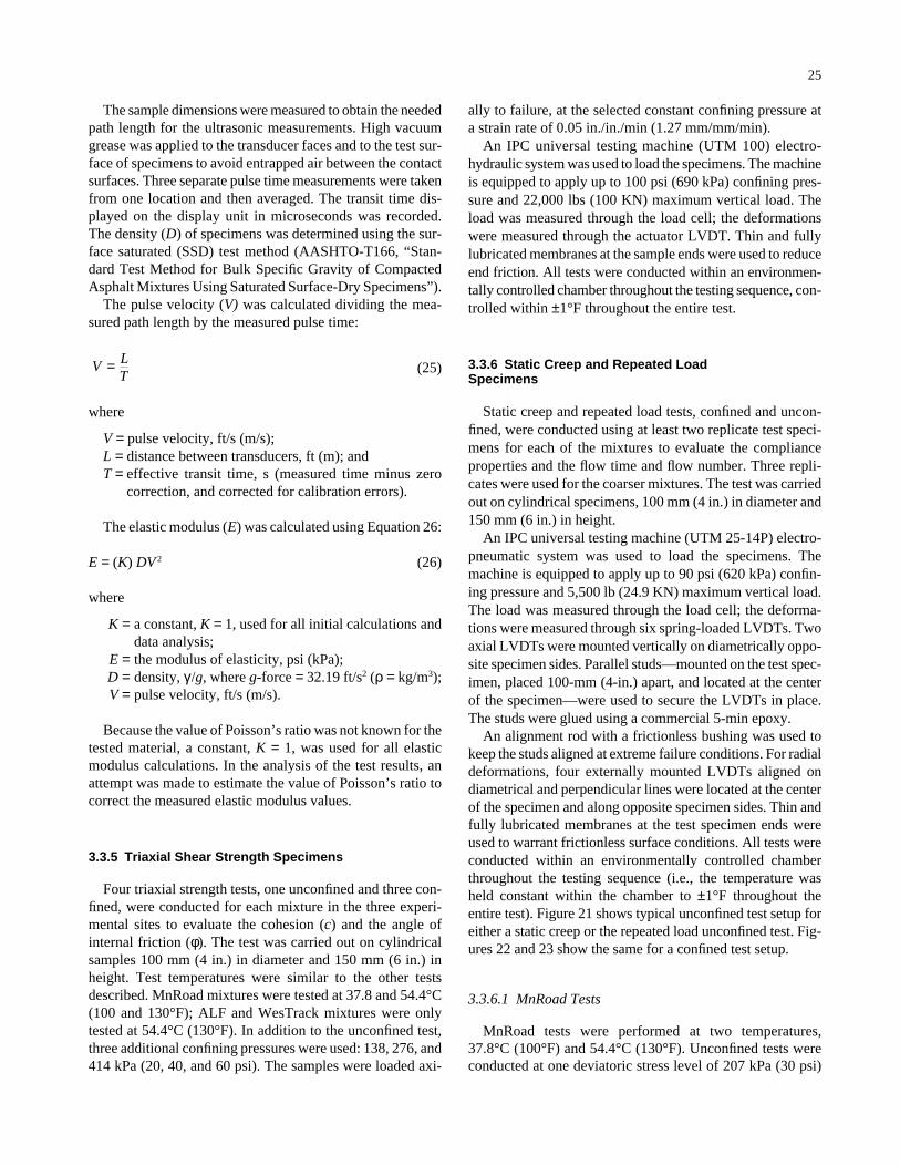
The sample dimensions were measured to obtain the neededpath length for the ultrasonic measurements. High vacuumgrease was applied to the transducer faces and to the test sur-face of specimens to avoid entrapped air between the contactsurfaces. Three separate pulse time measurements were takenfrom one location and then averaged. The transit time dis-played on the display unit in microseconds was recorded.The density (D) of specimens was determined using the sur-face saturated (SSD) test method (AASHTO-T166, “Stan-dard Test Method for Bulk Specific Gravity of CompactedAsphalt Mixtures Using Saturated Surface-Dry Specimens”).
The pulse velocity (V) was calculated dividing the mea-sured path length by the measured pulse time:
(25)
where
V = pulse velocity, ft/s (m/s);L = distance between transducers, ft (m); andT = effective transit time, s (measured time minus zero
correction, and corrected for calibration errors).
The elastic modulus (E) was calculated using Equation 26:
E = (K) DV 2 (26)
where
K = a constant, K = 1, used for all initial calculations anddata analysis;
E = the modulus of elasticity, psi (kPa);D = density, γ/g, where g-force = 32.19 ft/s2 (ρ = kg/m3);V = pulse velocity, ft/s (m/s).
Because the value of Poisson’s ratio was not known for thetested material, a constant, K = 1, was used for all elasticmodulus calculations. In the analysis of the test results, anattempt was made to estimate the value of Poisson’s ratio tocorrect the measured elastic modulus values.
3.3.5 Triaxial Shear Strength Specimens
Four triaxial strength tests, one unconfined and three con-fined, were conducted for each mixture in the three experi-mental sites to evaluate the cohesion (c) and the angle ofinternal friction (φ). The test was carried out on cylindricalsamples 100 mm (4 in.) in diameter and 150 mm (6 in.) inheight. Test temperatures were similar to the other testsdescribed. MnRoad mixtures were tested at 37.8 and 54.4°C(100 and 130°F); ALF and WesTrack mixtures were onlytested at 54.4°C (130°F). In addition to the unconfined test,three additional confining pressures were used: 138, 276, and414 kPa (20, 40, and 60 psi). The samples were loaded axi-
V LT
=
25
ally to failure, at the selected constant confining pressure ata strain rate of 0.05 in./in./min (1.27 mm/mm/min).
An IPC universal testing machine (UTM 100) electro-hydraulic system was used to load the specimens. The machineis equipped to apply up to 100 psi (690 kPa) confining pres-sure and 22,000 lbs (100 KN) maximum vertical load. Theload was measured through the load cell; the deformationswere measured through the actuator LVDT. Thin and fullylubricated membranes at the sample ends were used to reduceend friction. All tests were conducted within an environmen-tally controlled chamber throughout the testing sequence, con-trolled within ±1°F throughout the entire test.
3.3.6 Static Creep and Repeated LoadSpecimens
Static creep and repeated load tests, confined and uncon-fined, were conducted using at least two replicate test speci-mens for each of the mixtures to evaluate the complianceproperties and the flow time and flow number. Three repli-cates were used for the coarser mixtures. The test was carriedout on cylindrical specimens, 100 mm (4 in.) in diameter and150 mm (6 in.) in height.
An IPC universal testing machine (UTM 25-14P) electro-pneumatic system was used to load the specimens. Themachine is equipped to apply up to 90 psi (620 kPa) confin-ing pressure and 5,500 lb (24.9 KN) maximum vertical load.The load was measured through the load cell; the deforma-tions were measured through six spring-loaded LVDTs. Twoaxial LVDTs were mounted vertically on diametrically oppo-site specimen sides. Parallel studs—mounted on the test spec-imen, placed 100-mm (4-in.) apart, and located at the centerof the specimen—were used to secure the LVDTs in place.The studs were glued using a commercial 5-min epoxy.
An alignment rod with a frictionless bushing was used tokeep the studs aligned at extreme failure conditions. For radialdeformations, four externally mounted LVDTs aligned ondiametrical and perpendicular lines were located at the centerof the specimen and along opposite specimen sides. Thin andfully lubricated membranes at the test specimen ends wereused to warrant frictionless surface conditions. All tests wereconducted within an environmentally controlled chamberthroughout the testing sequence (i.e., the temperature washeld constant within the chamber to ±1°F throughout theentire test). Figure 21 shows typical unconfined test setup foreither a static creep or the repeated load unconfined test. Fig-ures 22 and 23 show the same for a confined test setup.
3.3.6.1 MnRoad Tests
MnRoad tests were performed at two temperatures,37.8°C (100°F) and 54.4°C (130°F). Unconfined tests wereconducted at one deviatoric stress level of 207 kPa (30 psi)
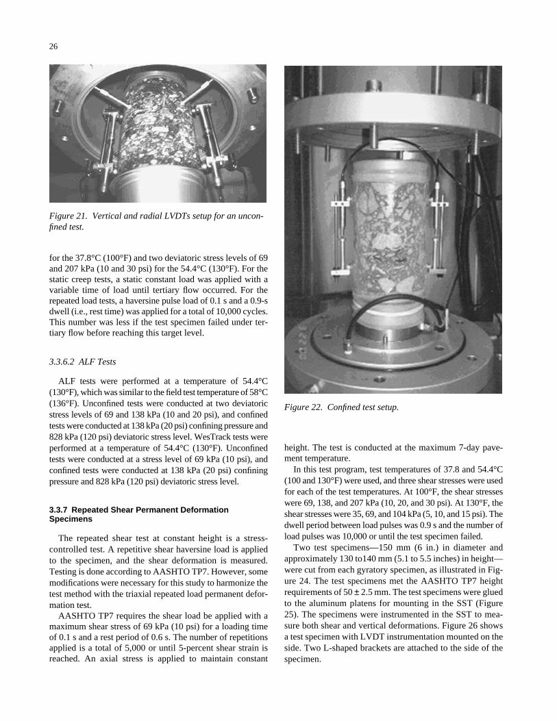
for the 37.8°C (100°F) and two deviatoric stress levels of 69and 207 kPa (10 and 30 psi) for the 54.4°C (130°F). For thestatic creep tests, a static constant load was applied with avariable time of load until tertiary flow occurred. For therepeated load tests, a haversine pulse load of 0.1 s and a 0.9-sdwell (i.e., rest time) was applied for a total of 10,000 cycles.This number was less if the test specimen failed under ter-tiary flow before reaching this target level.
3.3.6.2 ALF Tests
ALF tests were performed at a temperature of 54.4°C(130°F), which was similar to the field test temperature of 58°C(136°F). Unconfined tests were conducted at two deviatoricstress levels of 69 and 138 kPa (10 and 20 psi), and confinedtests were conducted at 138 kPa (20 psi) confining pressure and828 kPa (120 psi) deviatoric stress level. WesTrack tests wereperformed at a temperature of 54.4°C (130°F). Unconfinedtests were conducted at a stress level of 69 kPa (10 psi), andconfined tests were conducted at 138 kPa (20 psi) confiningpressure and 828 kPa (120 psi) deviatoric stress level.
3.3.7 Repeated Shear Permanent DeformationSpecimens
The repeated shear test at constant height is a stress-controlled test. A repetitive shear haversine load is appliedto the specimen, and the shear deformation is measured.Testing is done according to AASHTO TP7. However, somemodifications were necessary for this study to harmonize thetest method with the triaxial repeated load permanent defor-mation test.
AASHTO TP7 requires the shear load be applied with amaximum shear stress of 69 kPa (10 psi) for a loading timeof 0.1 s and a rest period of 0.6 s. The number of repetitionsapplied is a total of 5,000 or until 5-percent shear strain isreached. An axial stress is applied to maintain constant
26
height. The test is conducted at the maximum 7-day pave-ment temperature.
In this test program, test temperatures of 37.8 and 54.4°C(100 and 130°F) were used, and three shear stresses were usedfor each of the test temperatures. At 100°F, the shear stresseswere 69, 138, and 207 kPa (10, 20, and 30 psi). At 130°F, theshear stresses were 35, 69, and 104 kPa (5, 10, and 15 psi). Thedwell period between load pulses was 0.9 s and the number ofload pulses was 10,000 or until the test specimen failed.
Two test specimens—150 mm (6 in.) in diameter andapproximately 130 to140 mm (5.1 to 5.5 inches) in height—were cut from each gyratory specimen, as illustrated in Fig-ure 24. The test specimens met the AASHTO TP7 heightrequirements of 50 ± 2.5 mm. The test specimens were gluedto the aluminum platens for mounting in the SST (Figure25). The specimens were instrumented in the SST to mea-sure both shear and vertical deformations. Figure 26 showsa test specimen with LVDT instrumentation mounted on theside. Two L-shaped brackets are attached to the side of thespecimen.
Figure 21. Vertical and radial LVDTs setup for an uncon-fined test.
Figure 22. Confined test setup.
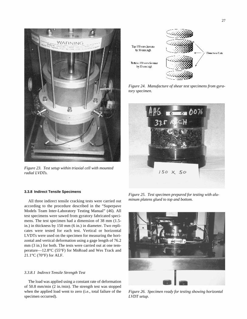
3.3.8 Indirect Tensile Specimens
All three indirect tensile cracking tests were carried outaccording to the procedure described in the “SuperpaveModels Team Inter-Laboratory Testing Manual” (46). Alltest specimens were sawed from gyratory fabricated speci-mens. The test specimen had a dimension of 38 mm (1.5-in.) in thickness by 150 mm (6 in.) in diameter. Two repli-cates were tested for each test. Vertical or horizontalLVDTs were used on the specimen for measuring the hori-zontal and vertical deformation using a gage length of 76.2mm (3 in.) for both. The tests were carried out at one tem-perature—12.8°C (55°F) for MnRoad and Wes Track and21.1°C (70°F) for ALF.
3.3.8.1 Indirect Tensile Strength Test
The load was applied using a constant rate of deformationof 50.8 mm/min (2 in./min). The strength test was stoppedwhen the applied load went to zero (i.e., total failure of thespecimen occurred).
27
Figure 23. Test setup within triaxial cell with mountedradial LVDTs.
Figure 24. Manufacture of shear test specimens from gyra-tory specimen.
Figure 25. Test specimen prepared for testing with alu-minum platens glued to top and bottom.
Figure 26. Specimen ready for testing showing horizontalLVDT setup.

3.3.8.2 Indirect Tensile Creep Test
The static creep test used in the study was one cycle load-unload. Two stress levels were used: a high stress level thatequaled 10 percent of the indirect tensile strength of thematerial and a low stress level that corresponded to 2 percentof the indirect tensile strength of the material. A 1,000-s staticloading time was used for the test followed by another 1,000s for unloading. The indirect tensile creep test was used toprovide the vertical and horizontal deformations as a func-tion of time. These deformations were then used to estimatethe creep compliance parameters, as presented in Chapter 2.
3.3.8.3 Indirect Tensile Fatigue Test
Eight to twelve replicates were tested for each of theexperimental sites sections considered in the study. The load-ing pattern followed in the fatigue test was a haversine load
28
with a rest period. The loading period selected was 0.1 s. Therest duration selected was 0.4 s. The stress amplitude waskept constant and corresponding deformations were recordedat different times. The load was applied until the sample frac-tured along the vertical diameter.
In the indirect fatigue test, horizontal deformations (i.e.,strains) are recorded as a function of load repetitions. Thismethod of recording allows the resilient modulus to be esti-mated as a function of a specific load cycle. Each specimenis subjected to a different level of stress (or strain) so that theNf or N50 will result in a range of values for fracture life. Thiswill allow for the development of the classic fatigue rela-tionship between Nf and σ (stress) or ε (strain) on a log–logmodel form. Different stress levels were used for each sam-ple in order to obtain fatigue life between 100 to 100,000load cycles. These fracture relations then can be evaluated tosee whether a relationship exists between these parametersand the fatigue cracking measured from the road tests.
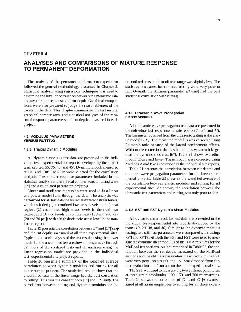
29
CHAPTER 4
ANALYSES AND COMPARISONS OF MIXTURE RESPONSE TO PERMANENT DEFORMATION
The analysis of the permanent deformation experimentfollowed the general methodology discussed in Chapter 3.Statistical analysis using regression techniques was used todetermine the level of correlation between the measured lab-oratory mixture response and rut depth. Graphical compar-isons were also prepared to judge the reasonableness of thetrends in the data. This chapter summarizes the test results,graphical comparisons, and statistical analyses of the mea-sured response parameters and rut depths measured in eachproject.
4.1 MODULUS PARAMETERS VERSUS RUTTING
4.1.1 Triaxial Dynamic Modulus
All dynamic modulus test data are presented in the indi-vidual test–experimental site reports developed by the projectteam (25, 26, 35, 36, 45, and 46). Dynamic moduli measuredat 100 and 130°F at 5 Hz were selected for the correlationanalysis. The mixture response parameters included in thestatistical analysis and graphical comparisons to rutting were|E*| and a calculated parameter |E*|/sinφ.
Linear and nonlinear regression were used to fit a linearand power model form through the data. The analysis wasperformed for all test data measured at different stress levels,which included (1) unconfined low stress levels in the linearregion; (2) unconfined high stress levels in the nonlinearregion; and (3) two levels of confinement (138 and 206 kPa[20 and 30 psi]) with a high deviatoric stress level in the non-linear region.
Table 19 presents the correlation between |E*|and |E*|/sinφand the rut depths measured at all three experimental sites.Typical plots and analyses of the test results using the powermodel for the unconfined test are shown in Figures 27 through32. Plots of the confined tests and all analyses using thelinear regression model are provided in the individualtest–experimental site project reports.
Table 20 presents a summary of the weighted averagecorrelation between dynamic modulus and rutting for allexperimental projects. The statistical results show that theunconfined tests in the linear range had the best correlationto rutting. This was the case for both |E*| and| E*|/sinφ. Thecorrelation between rutting and dynamic modulus for the
unconfined tests in the nonlinear range was slightly less. Thestatistical measures for confined testing were very poor tofair. Overall, the stiffness parameter |E*|/sinφ had the beststatistical correlation with rutting.
4.1.2 Ultrasonic Wave Propagation Elastic Modulus
All ultrasonic wave propagation test data are presented inthe individual test–experimental site reports (24, 34, and 44).The parameter obtained from the ultrasonic testing is the elas-tic modulus, Ed. The measured modulus was corrected usingPoisson’s ratio because of the lateral confinement effects.Without the correction, the elastic modulus was much largerthan the dynamic modulus, |E*|. Table 21 shows two othermoduli, ECORA and ECORB. These moduli were corrected usingMethods A and B as is described in the individual site reports.
Table 21 presents the correlation between rut depths andthe three wave-propagation parameters for all three experi-mental projects. Table 22 presents the weighted average ofthe correlation between elastic modulus and rutting for allexperimental sites. As shown, the correlation between theultrasonic test parameters and rutting was only poor to fair.
4.1.3 SST and FST Dynamic Shear Modulus
All dynamic shear modulus test data are presented in theindividual test–experimental site reports developed by theteam (19, 20, 30, and 40). Similar to the dynamic modulustesting, two stiffness parameters were compared with rutting:|G*| and |G*|/sinφ. Both the SST and FST were used to mea-sure the dynamic shear modulus of the HMA mixtures for theMnRoad test sections. As is summarized in Table 23, the cor-relation between the rut depths measured on the MnRoadsections and the stiffness parameters measured with the FSTwere very poor. As a result, the FST was dropped from fur-ther evaluation and from use on the other experimental sites.
The SST was used to measure the two stiffness parametersat three strain amplitudes: 100, 150, and 200 microstrains.Table 24 shows the correlation of |G*| and |G*|/sinφ mea-sured at all strain amplitudes to rutting for all three experi-
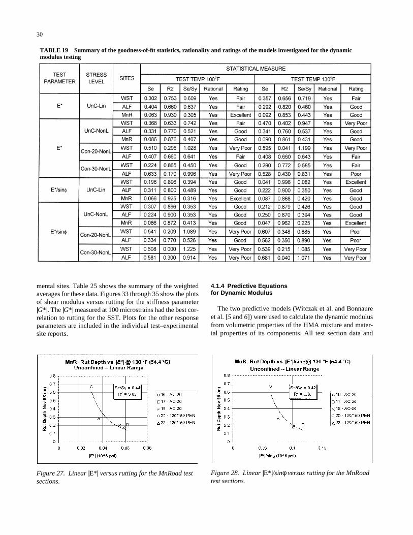
mental sites. Table 25 shows the summary of the weightedaverages for these data. Figures 33 through 35 show the plotsof shear modulus versus rutting for the stiffness parameter|G*|. The |G*| measured at 100 microstrains had the best cor-relation to rutting for the SST. Plots for the other responseparameters are included in the individual test–experimentalsite reports.
30
4.1.4 Predictive Equations for Dynamic Modulus
The two predictive models (Witczak et al. and Bonnaureet al. [5 and 6]) were used to calculate the dynamic modulusfrom volumetric properties of the HMA mixture and mater-ial properties of its components. All test section data and
TABLE 19 Summary of the goodness-of-fit statistics, rationality and ratings of the models investigated for the dynamicmodulus testing
Figure 27. Linear |E*| versus rutting for the MnRoad testsections.
Figure 28. Linear |E*|/sinφversus rutting for the MnRoadtest sections.
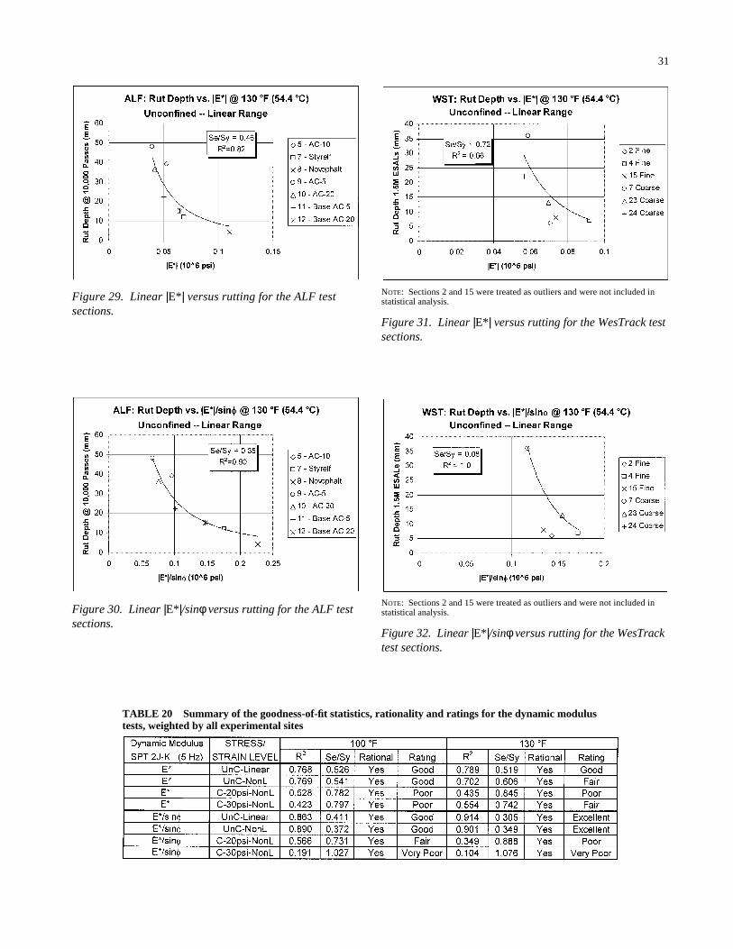
31
Figure 29. Linear |E*| versus rutting for the ALF test sections.
Figure 30. Linear |E*|/sinφversus rutting for the ALF testsections.
Figure 31. Linear |E*| versus rutting for the WesTrack testsections.
NOTE: Sections 2 and 15 were treated as outliers and were not included instatistical analysis.
NOTE: Sections 2 and 15 were treated as outliers and were not included instatistical analysis.
Figure 32. Linear |E*|/sinφversus rutting for the WesTracktest sections.
TABLE 20 Summary of the goodness-of-fit statistics, rationality and ratings for the dynamic modulustests, weighted by all experimental sites
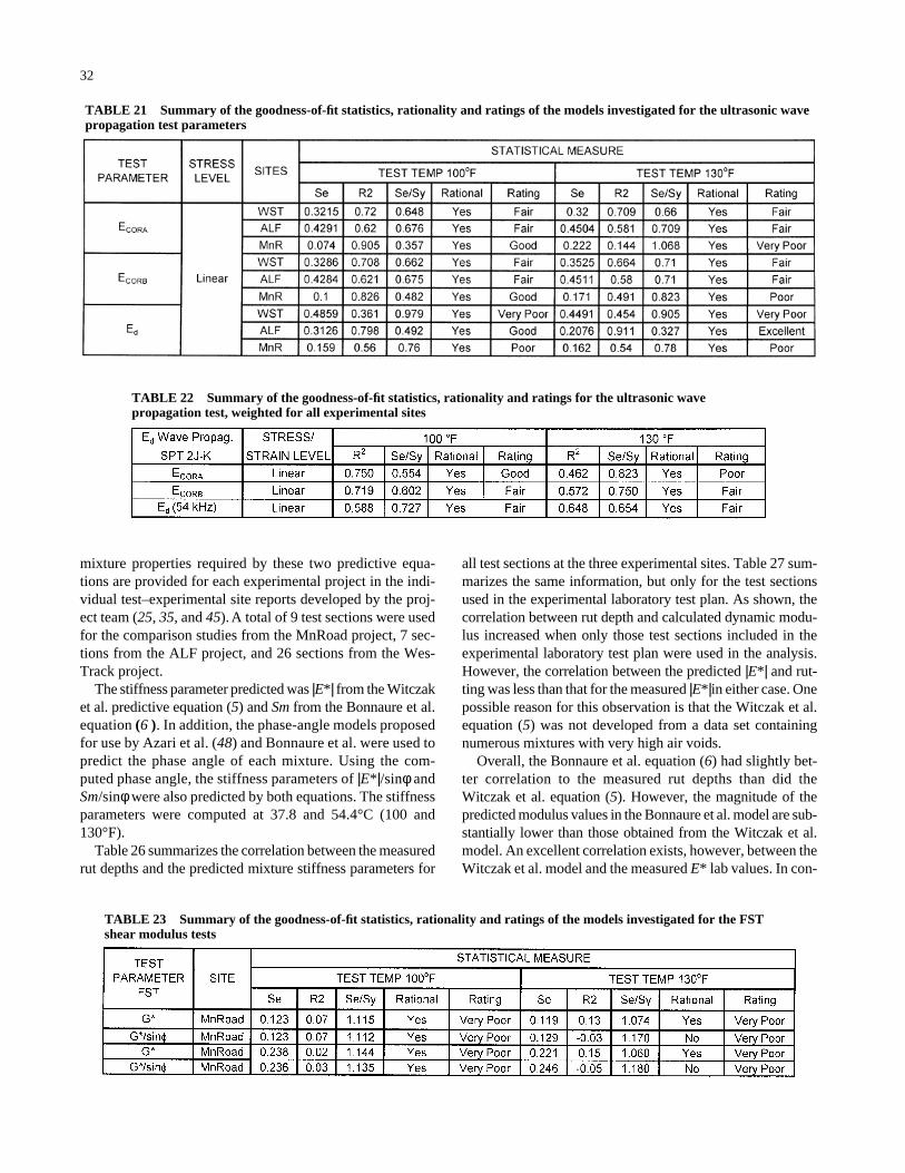
mixture properties required by these two predictive equa-tions are provided for each experimental project in the indi-vidual test–experimental site reports developed by the proj-ect team (25, 35, and 45). A total of 9 test sections were usedfor the comparison studies from the MnRoad project, 7 sec-tions from the ALF project, and 26 sections from the Wes-Track project.
The stiffness parameter predicted was |E*| from the Witczaket al. predictive equation (5) and Sm from the Bonnaure et al.equation (6 ). In addition, the phase-angle models proposedfor use by Azari et al. (48) and Bonnaure et al. were used topredict the phase angle of each mixture. Using the com-puted phase angle, the stiffness parameters of |E*|/sinφandSm/sinφwere also predicted by both equations. The stiffnessparameters were computed at 37.8 and 54.4°C (100 and130°F).
Table 26 summarizes the correlation between the measuredrut depths and the predicted mixture stiffness parameters for
32
all test sections at the three experimental sites. Table 27 sum-marizes the same information, but only for the test sectionsused in the experimental laboratory test plan. As shown, thecorrelation between rut depth and calculated dynamic modu-lus increased when only those test sections included in theexperimental laboratory test plan were used in the analysis.However, the correlation between the predicted |E*| and rut-ting was less than that for the measured |E*|in either case. Onepossible reason for this observation is that the Witczak et al.equation (5) was not developed from a data set containingnumerous mixtures with very high air voids.
Overall, the Bonnaure et al. equation (6) had slightly bet-ter correlation to the measured rut depths than did theWitczak et al. equation (5). However, the magnitude of thepredicted modulus values in the Bonnaure et al. model are sub-stantially lower than those obtained from the Witczak et al.model. An excellent correlation exists, however, between theWitczak et al. model and the measured E* lab values. In con-
TABLE 23 Summary of the goodness-of-fit statistics, rationality and ratings of the models investigated for the FSTshear modulus tests
TABLE 21 Summary of the goodness-of-fit statistics, rationality and ratings of the models investigated for the ultrasonic wavepropagation test parameters
TABLE 22 Summary of the goodness-of-fit statistics, rationality and ratings for the ultrasonic wavepropagation test, weighted for all experimental sites
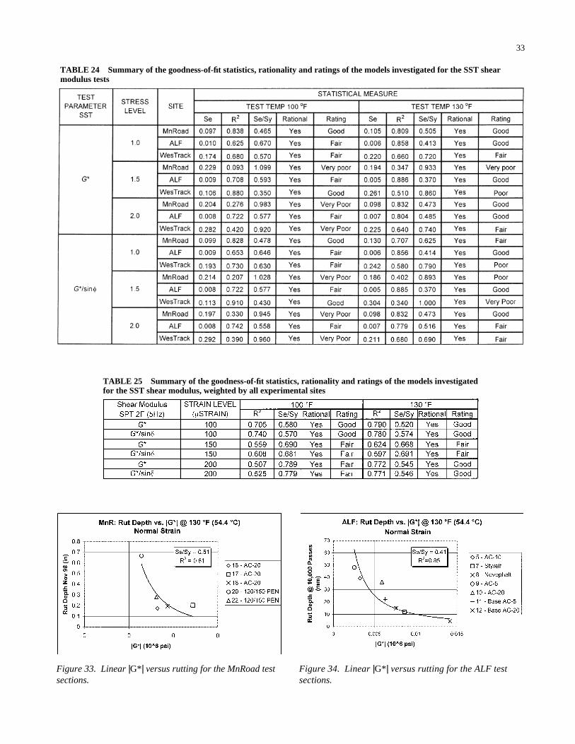
33
TABLE 24 Summary of the goodness-of-fit statistics, rationality and ratings of the models investigated for the SST shearmodulus tests
TABLE 25 Summary of the goodness-of-fit statistics, rationality and ratings of the models investigatedfor the SST shear modulus, weighted by all experimental sites
Figure 34. Linear |G*| versus rutting for the ALF testsections.
Figure 33. Linear |G*| versus rutting for the MnRoad testsections.
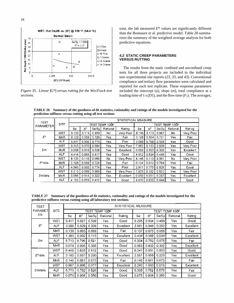
34
trast, the lab measured E* values are significantly differentthan the Bonnaure et al. predictive model. Table 28 summa-rizes the summary of the weighted average analysis for bothpredictive equations.
4.2 STATIC CREEP PARAMETERS VERSUS RUTTING
The results from the static confined and unconfined creeptests for all three projects are included in the individualtest–experimental site reports (23, 33, and 43). Conventionalcompliance and tertiary flow parameters were calculated andreported for each test replicate. These response parametersincluded the intercept (a), slope (m), total compliance at aloading time of 1 s (D1), and the flow time (FT). The averages,
Figure 35. Linear |G*| versus rutting for the WesTrack testsections.
TABLE 27 Summary of the goodness-of-fit statistics, rationality and ratings of the models investigated for thepredictive stiffness versus rutting using all laboratory test sections
TABLE 26 Summary of the goodness-of-fit statistics, rationality and ratings of the models investigated for theprediction stiffness versus rutting using all test sections

standard deviations, and coefficient of variation from the tworeplicates are included in the individual test–experimental sitereports.
Statistical analyses were completed on all response param-eters to determine how well these parameters correlated to themeasured rut depths. Tables 29 and 30 summarize the good-ness-of-fit statistics, the rationality of the trends for the uncon-
35
fined and confined test results, and the subjective ratings of thecorrelations for each response parameter and regressionmodel. Table 31 presents the final rating weighted by all exper-imental projects.
The flow time was the highest ranked test parameter forthe static creep test. Figures 36 through 41 are plots of themeasured rut depths for each test section versus the flow time
TABLE 28 Weighted summary of the goodness-of-fit statistics, rationality and ratings for thepredictive stiffness versus rutting using laboratory test sections
TABLE 29 Summary of the goodness-of-fit statistics, rationality and ratings of the models investigated for the unconfinedstatic creep–flow time test
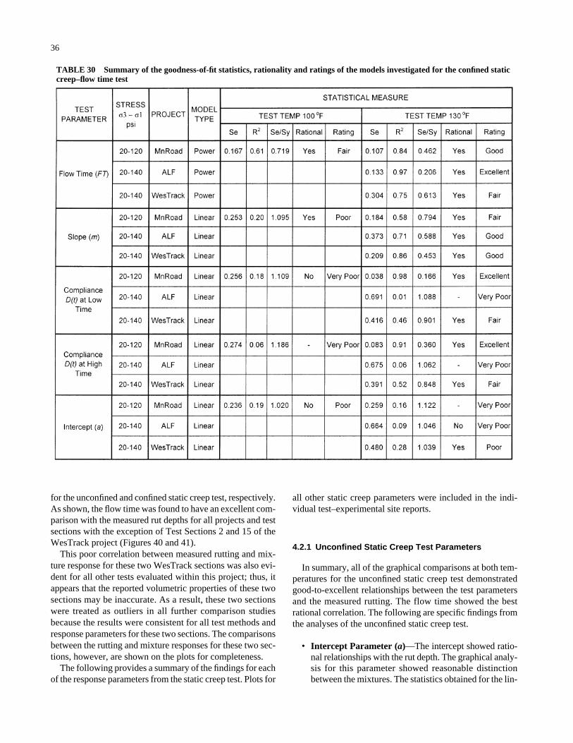
for the unconfined and confined static creep test, respectively.As shown, the flow time was found to have an excellent com-parison with the measured rut depths for all projects and testsections with the exception of Test Sections 2 and 15 of theWesTrack project (Figures 40 and 41).
This poor correlation between measured rutting and mix-ture response for these two WesTrack sections was also evi-dent for all other tests evaluated within this project; thus, itappears that the reported volumetric properties of these twosections may be inaccurate. As a result, these two sectionswere treated as outliers in all further comparison studiesbecause the results were consistent for all test methods andresponse parameters for these two sections. The comparisonsbetween the rutting and mixture responses for these two sec-tions, however, are shown on the plots for completeness.
The following provides a summary of the findings for eachof the response parameters from the static creep test. Plots for
36
all other static creep parameters were included in the indi-vidual test–experimental site reports.
4.2.1 Unconfined Static Creep Test Parameters
In summary, all of the graphical comparisons at both tem-peratures for the unconfined static creep test demonstratedgood-to-excellent relationships between the test parametersand the measured rutting. The flow time showed the bestrational correlation. The following are specific findings fromthe analyses of the unconfined static creep test.
• Intercept Parameter (a)—The intercept showed ratio-nal relationships with the rut depth. The graphical analy-sis for this parameter showed reasonable distinctionbetween the mixtures. The statistics obtained for the lin-
TABLE 30 Summary of the goodness-of-fit statistics, rationality and ratings of the models investigated for the confined staticcreep–flow time test
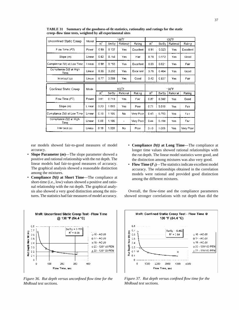
ear models showed fair-to-good measures of modelaccuracy.
• Slope Parameter (m)—The slope parameter showed apositive and rational relationship with the rut depth. Thelinear models had fair-to-good measures of accuracy.The graphical analysis showed a reasonable distinctionamong the mixtures.
• Compliance D(t) at Short Time—The compliance atshort-time (i.e., low) values showed a positive and ratio-nal relationship with the rut depth. The graphical analy-sis also showed a very good distinction among the mix-tures. The statistics had fair measures of model accuracy.
37
• Compliance D(t) at Long Time—The compliance atlonger time values showed rational relationships withthe rut depth. The linear model statistics were good, andthe distinction among mixtures was also very good.
• Flow Time (FT)—The statistics indicate excellent modelaccuracy. The relationships obtained in the correlationmodels were rational and provided good distinctionamong the different mixtures.
Overall, the flow-time and the compliance parametersshowed stronger correlations with rut depth than did the
TABLE 31 Summary of the goodness-of-fit statistics, rationality and ratings for the staticcreep–flow time tests, weighted by all experimental sites
Figure 37. Rut depth versus confined flow time for theMnRoad test sections.
Figure 36. Rut depth versus unconfined flow time for theMnRoad test sections.

intercept and slope parameters when analyzed separately.All of the models were rational in that the flow time decreasedas the rut depth increased. The flow-time models showed avery good distinction among the different mixtures. Poor-performing mixtures had the lowest flow time (i.e., the short-est time to failure); the good-performing mixtures had thelargest flow time (i.e., the longest time to failure).
The ALF experiment provided a particularly good assess-ment of the flow-time parameter. The high-and-wide rangeof air void levels present among the different ALF mixturesmight be expected to interfere with the relationship to theperformance because densification has a strong influence onparameters such as the intercept and compliance. The densi-fication range, however, did not affect the onset of tertiaryflow as can be observed by the excellent relationship that wasfound between the flow parameters and the observed sectionrutting.
38
4.2.2 Confined Static Creep Test Parameters
All of the plots for the confined testing at 130°F (exceptfor the intercept) demonstrated fair-to-good relationshipsbetween the test parameters and the permanent deformation(i.e., rutting) behavior in the field. The following are specificfindings from the analyses of the confined static creep test.
• Intercept Parameter (a)—The intercept did not showa rational relationship with the rut depth and had verypoor measures of model accuracy. No clear trend wasobserved with the rut-depth measurements.
• Slope Parameter (m)—The slope parameter showedpositive and rational relationships with the rut depth.The linear-model statistics were indicative of good mea-sures of model accuracy.
Figure 41. Rut depth versus confined flow time for theWesTrack test sections.
Figure 39. Rut depth versus confined flow time for the ALFtest sections.
NOTE: Sections 2 and 15 treated as outliers and are not included in statisticalanalysis.Figure 38. Rut depth versus unconfined flow time for the
ALF test sections.Figure 40. Rut depth versus unconfined flow time for theWesTrack test sections.
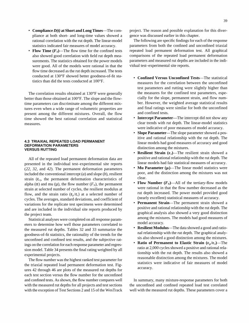
• Compliance D(t) at Short and Long Times—The com-pliance at both short- and long-time values showed arational correlation with the rut depth. The linear-modelstatistics indicated fair measures of model accuracy.
• Flow Time (FT)—The flow time for the confined testsalso showed good correlation with field rut depth mea-surements. The statistics obtained for the power modelswere good. All of the models were rational in that theflow time decreased as the rut depth increased. The testsconducted at 130°F showed better goodness-of-fit sta-tistics than did the tests conducted at 100°F.
The correlation results obtained at 130°F were generallybetter than those obtained at 100°F. The slope and the flow-time parameters can discriminate among the different mix-tures even when a wide range of volumetric properties arepresent among the different mixtures. Overall, the flowtime showed the best rational correlation and statisticalmeasures.
4.3 TRIAXIAL REPEATED LOAD PERMANENTDEFORMATION PARAMETERS VERSUS RUTTING
All of the repeated load permanent deformation data arepresented in the individual test–experimental site reports(22, 32, and 42). The permanent deformation parametersincluded the conventional intercept (a) and slope (b), resilientstrain (εr), the permanent deformation characteristics ofalpha (α) and mu (µ), the flow number (FN), the permanentstrain at selected number of cycles, the resilient modulus atflow, and the strain ratio (εp/εr) at a selected number ofcycles. The averages, standard deviations, and coefficient ofvariations for the replicate test specimens were determinedand are included in the individual site reports produced bythe project team.
Statistical analyses were completed on all response param-eters to determine how well those parameters correlated tothe measured rut depths. Tables 32 and 33 summarize thegoodness-of-fit statistics, the rationality of the trends for theunconfined and confined test results, and the subjective rat-ings on the correlation for each response parameter and regres-sion model. Table 34 presents the final rating weighted by allexperimental projects.
The flow number was the highest ranked test parameter forthe triaxial repeated load permanent deformation test. Fig-ures 42 through 46 are plots of the measured rut depths foreach test section versus the flow number for the unconfinedand confined tests. As shown, the flow number compares wellwith the measured rut depths for all projects and test sectionswith the exception of Test Sections 2 and 15 of the WesTrack
39
project. The reason and possible explanation for this diver-gence was discussed earlier in this chapter.
The following are specific findings for each of the responseparameters from both the confined and unconfined triaxialrepeated load permanent deformation test. All graphicalcomparisons of the repeated load permanent deformationparameters and measured rut depths are included in the indi-vidual test–experimental site reports.
• Confined Versus Unconfined Tests—The statisticalmeasures for the correlation between the unconfinedtest parameters and rutting were slightly higher thanthe measures for the confined test parameters, espe-cially for the slope, permanent strain, and flow num-ber. However, the weighted average statistical resultsand final ratings were similar for both the unconfinedand confined tests.
• Intercept Parameter—The intercept did not show anyclear trends with rut depth. The linear-model statisticswere indicative of poor measures of model accuracy.
• Slope Parameter—The slope parameter showed a pos-itive and rational relationship with the rut depth. Thelinear models had good measures of accuracy and gooddistinction among the mixtures.
• Resilient Strain (�r)—The resilient strain showed apositive and rational relationship with the rut depth. Thelinear models had fair statistical measures of accuracy.
• Mu Parameter (�)—The linear model statistics werepoor, and the distinction among the mixtures was notclear.
• Flow Number (FN)—All of the tertiary-flow modelswere rational in that the flow number decreased as therut depth increased. The power model provided good(nearly excellent) statistical measures of accuracy.
• Permanent Strain—The permanent strain showed apositive and rational relationship with the rut depth. Thegraphical analysis also showed a very good distinctionamong the mixtures. The models had good measures ofmodel accuracy.
• Resilient Modulus—The data showed a good and ratio-nal relationship with the rut depth. The graphical analy-sis also showed a good distinction among the mixtures.
• Ratio of Permanent to Elastic Strain (�p /�r)—Theratio at 2,000 cycles showed a positive and rational rela-tionship with the rut depth. The results also showed areasonable distinction among the mixtures. The modelstatistics were indicative of fair measures of modelaccuracy.
In summary, many mixture-response parameters for boththe unconfined and confined repeated load test correlatedwell with the measured rut depths. These parameters cover a
wide range of material behavior from elastic properties, suchas the resilient modulus, to plastic properties, such as tertiaryflow. Overall, the slope, permanent strain, and the flow num-ber showed good correspondence with rut depth. Amongthese parameters, the flow number had the best statisticalmeasures.
40
4.4 SST REPEATED LOAD PERMANENTDEFORMATION PARAMETERS VERSUS RUTTING
All of the shear repeated load permanent deformation dataare presented in the individual test–experimental site reports(21, 31, and 41). The response parameters for the repeated
TABLE 32 Summary of the goodness-of-fit statistics, rationality and ratings of the models investigated for theunconfined repeated load tests
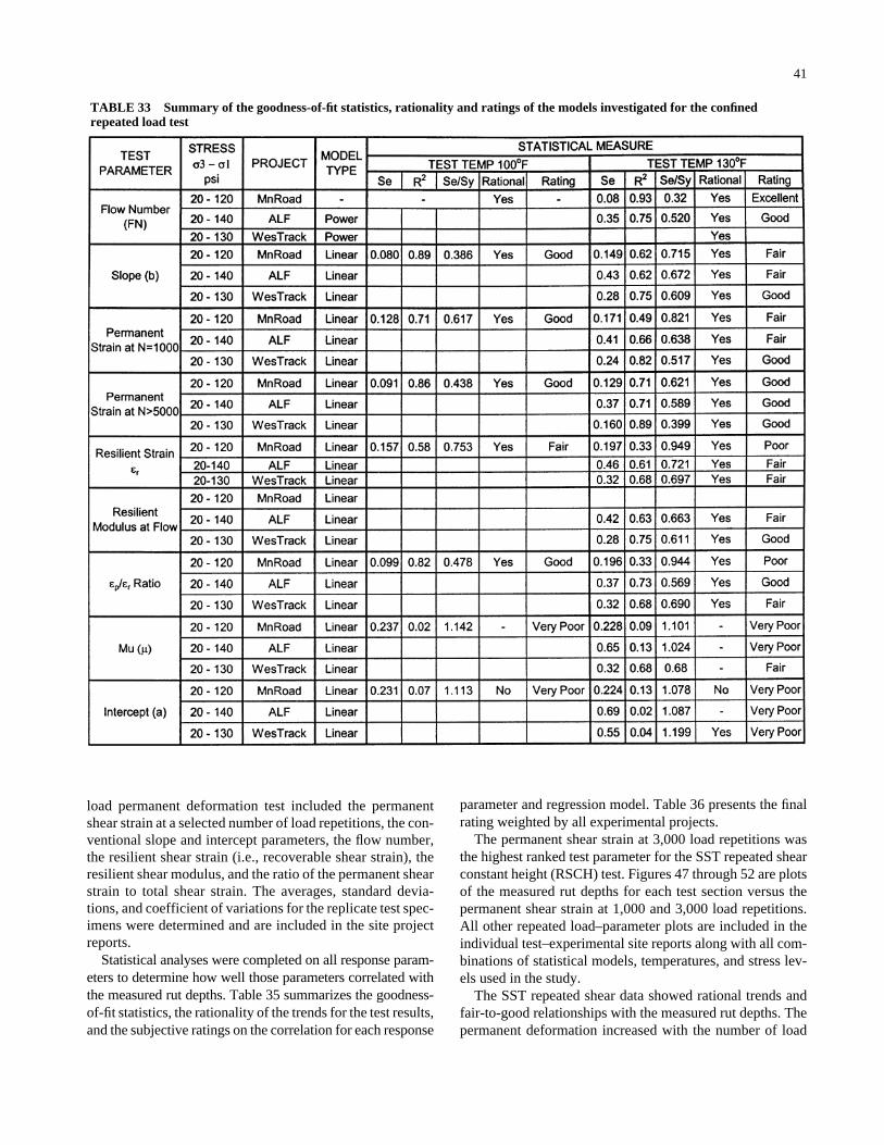
load permanent deformation test included the permanentshear strain at a selected number of load repetitions, the con-ventional slope and intercept parameters, the flow number,the resilient shear strain (i.e., recoverable shear strain), theresilient shear modulus, and the ratio of the permanent shearstrain to total shear strain. The averages, standard devia-tions, and coefficient of variations for the replicate test spec-imens were determined and are included in the site projectreports.
Statistical analyses were completed on all response param-eters to determine how well those parameters correlated withthe measured rut depths. Table 35 summarizes the goodness-of-fit statistics, the rationality of the trends for the test results,and the subjective ratings on the correlation for each response
41
parameter and regression model. Table 36 presents the finalrating weighted by all experimental projects.
The permanent shear strain at 3,000 load repetitions wasthe highest ranked test parameter for the SST repeated shearconstant height (RSCH) test. Figures 47 through 52 are plotsof the measured rut depths for each test section versus thepermanent shear strain at 1,000 and 3,000 load repetitions.All other repeated load–parameter plots are included in theindividual test–experimental site reports along with all com-binations of statistical models, temperatures, and stress lev-els used in the study.
The SST repeated shear data showed rational trends andfair-to-good relationships with the measured rut depths. Thepermanent deformation increased with the number of load
TABLE 33 Summary of the goodness-of-fit statistics, rationality and ratings of the models investigated for the confinedrepeated load test
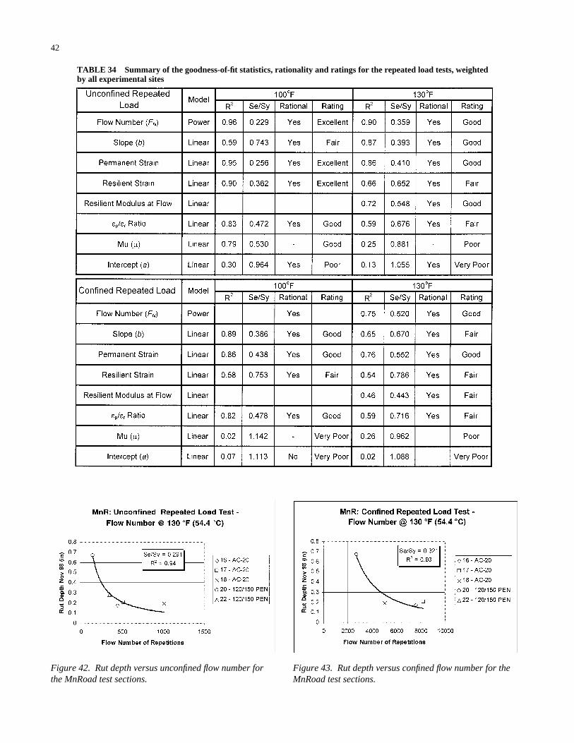
TABLE 34 Summary of the goodness-of-fit statistics, rationality and ratings for the repeated load tests, weightedby all experimental sites
42
Figure 43. Rut depth versus confined flow number for theMnRoad test sections.
Figure 42. Rut depth versus unconfined flow number forthe MnRoad test sections.
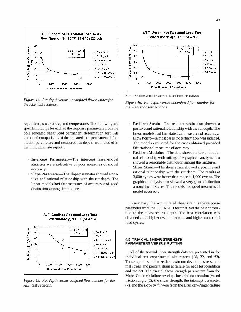
repetitions, shear stress, and temperature. The following arespecific findings for each of the response parameters from theSST repeated shear load permanent deformation test. Allgraphical comparisons of the repeated load permanent defor-mation parameters and measured rut depths are included inthe individual site reports.
• Intercept Parameter—The intercept linear-modelstatistics were indicative of poor measures of modelaccuracy.
• Slope Parameter—The slope parameter showed a pos-itive and rational relationship with the rut depth. Thelinear models had fair measures of accuracy and gooddistinction among the mixtures.
43
• Resilient Strain—The resilient strain also showed apositive and rational relationship with the rut depth. Thelinear models had fair statistical measures of accuracy.
• Flow Point—In most cases, no tertiary flow was induced.The models evaluated for the cases obtained providedfair statistical measures of accuracy.
• Resilient Modulus—The data showed a fair and ratio-nal relationship with rutting. The graphical analysis alsoshowed a reasonable distinction among the mixtures.
• Shear Strain—The shear strain showed a positive andrational relationship with the rut depth. The results at3,000 cycles were better than those at 1,000 cycles. Thegraphical analysis also showed a very good distinctionamong the mixtures. The models had good measures ofmodel accuracy.
In summary, the accumulated shear strain is the responseparameter from the SST RSCH test that had the best correla-tion to the measured rut depth. The best correlation wasobtained at the higher test temperature and higher number ofload cycles.
4.5 TRIAXIAL SHEAR STRENGTHPARAMETERS VERSUS RUTTING
All of the triaxial shear strength data are presented in theindividual test–experimental site reports (18, 29, and 40).These reports summarize the maximum deviatoric stress, nor-mal stress, and percent strain at failure for each test conditionand project. The triaxial shear strength parameters from theMohr–Coulomb failure envelope included the cohesion (c) andfriction angle (φ); the shear strength, the intercept parameter(k), and the slope (γ1/2) were from the Drucker–Prager failure
Figure 45. Rut depth versus confined flow number for theALF test sections.
Figure 44. Rut depth versus unconfined flow number forthe ALF test sections.
NOTE: Sections 2 and 15 were excluded from the analysis.
Figure 46. Rut depth versus unconfined flow number forthe WesTrack test sections.
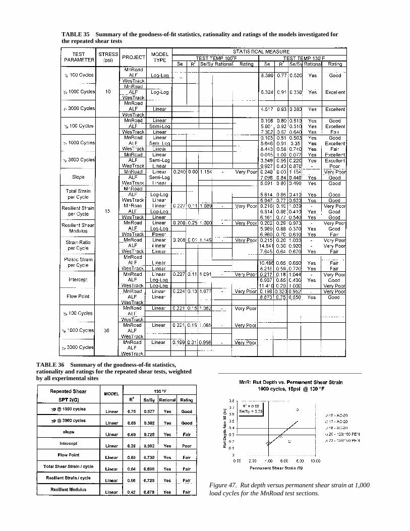
TABLE 35 Summary of the goodness-of-fit statistics, rationality and ratings of the models investigated forthe repeated shear tests
TABLE 36 Summary of the goodness-of-fit statistics,rationality and ratings for the repeated shear tests, weightedby all experimental sites
Figure 47. Rut depth versus permanent shear strain at 1,000load cycles for the MnRoad test sections.
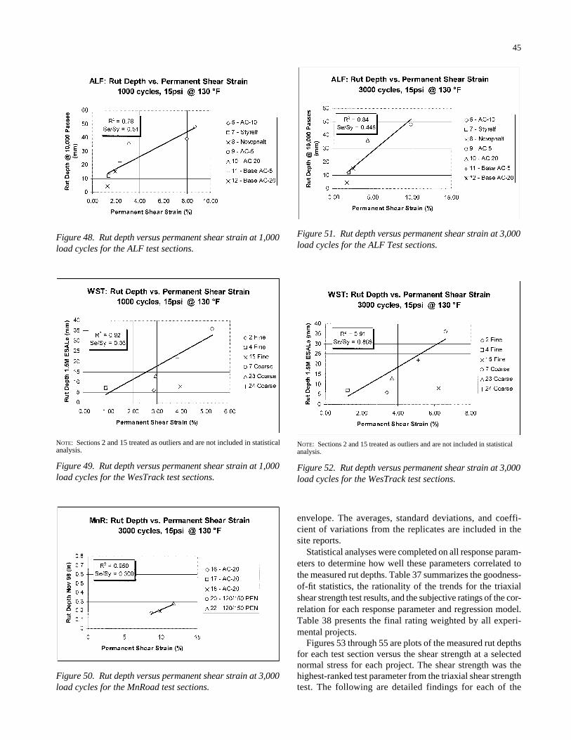
45
envelope. The averages, standard deviations, and coeffi-cient of variations from the replicates are included in thesite reports.
Statistical analyses were completed on all response param-eters to determine how well these parameters correlated tothe measured rut depths. Table 37 summarizes the goodness-of-fit statistics, the rationality of the trends for the triaxialshear strength test results, and the subjective ratings of the cor-relation for each response parameter and regression model.Table 38 presents the final rating weighted by all experi-mental projects.
Figures 53 through 55 are plots of the measured rut depthsfor each test section versus the shear strength at a selectednormal stress for each project. The shear strength was thehighest-ranked test parameter from the triaxial shear strengthtest. The following are detailed findings for each of the
Figure 51. Rut depth versus permanent shear strain at 3,000load cycles for the ALF Test sections.
Figure 48. Rut depth versus permanent shear strain at 1,000load cycles for the ALF test sections.
Figure 50. Rut depth versus permanent shear strain at 3,000load cycles for the MnRoad test sections.
NOTE: Sections 2 and 15 treated as outliers and are not included in statisticalanalysis.
Figure 49. Rut depth versus permanent shear strain at 1,000load cycles for the WesTrack test sections.
NOTE: Sections 2 and 15 treated as outliers and are not included in statisticalanalysis.
Figure 52. Rut depth versus permanent shear strain at 3,000load cycles for the WesTrack test sections.
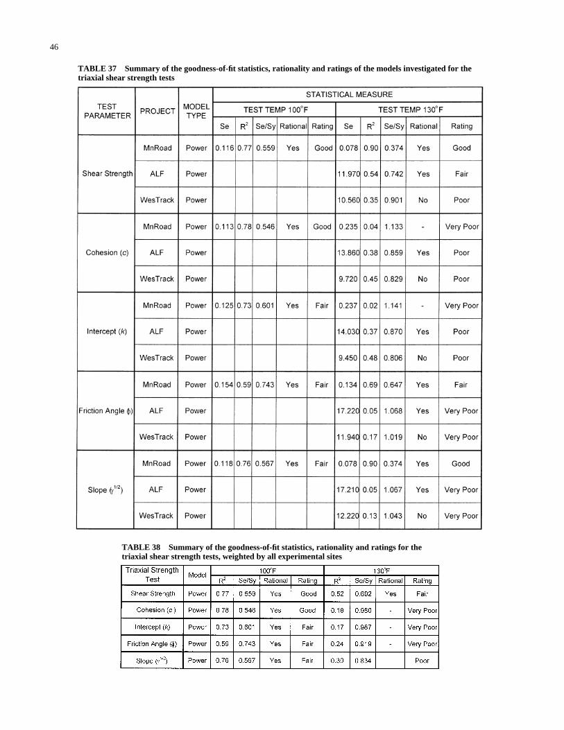
46
TABLE 38 Summary of the goodness-of-fit statistics, rationality and ratings for thetriaxial shear strength tests, weighted by all experimental sites
TABLE 37 Summary of the goodness-of-fit statistics, rationality and ratings of the models investigated for thetriaxial shear strength tests
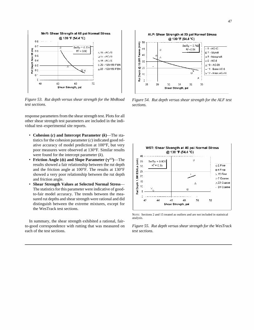
47
response parameters from the shear strength test. Plots for allother shear strength test parameters are included in the indi-vidual test–experimental site reports.
• Cohesion (c) and Intercept Parameter (k)—The sta-tistics for the cohesion parameter (c) indicated good rel-ative accuracy of model prediction at 100°F, but verypoor measures were observed at 130°F. Similar resultswere found for the intercept parameter (k).
• Friction Angle (�) and Slope Parameter (�1/2)—Theresults showed a fair relationship between the rut depthand the friction angle at 100°F. The results at 130°Fshowed a very poor relationship between the rut depthand friction angle.
• Shear Strength Values at Selected Normal Stress—The statistics for this parameter were indicative of good-to-fair model accuracy. The trends between the mea-sured rut depths and shear strength were rational and diddistinguish between the extreme mixtures, except forthe WesTrack test sections.
In summary, the shear strength exhibited a rational, fair-to-good correspondence with rutting that was measured oneach of the test sections.
Figure 54. Rut depth versus shear strength for the ALF testsections.
Figure 53. Rut depth versus shear strength for the MnRoadtest sections.
NOTE: Sections 2 and 15 treated as outliers and are not included in statisticalanalysis.
Figure 55. Rut depth versus shear strength for the WesTracktest sections.
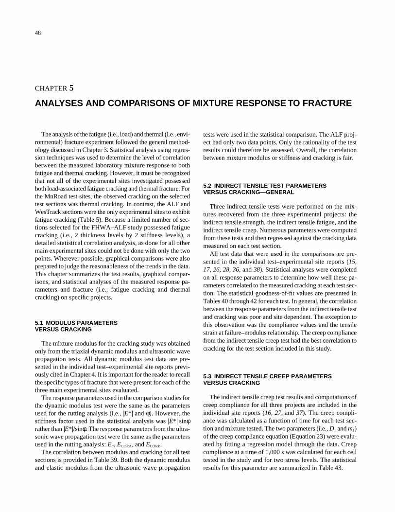
48
CHAPTER 5
ANALYSES AND COMPARISONS OF MIXTURE RESPONSE TO FRACTURE
The analysis of the fatigue (i.e., load) and thermal (i.e., envi-ronmental) fracture experiment followed the general method-ology discussed in Chapter 3. Statistical analysis using regres-sion techniques was used to determine the level of correlationbetween the measured laboratory mixture response to bothfatigue and thermal cracking. However, it must be recognizedthat not all of the experimental sites investigated possessedboth load-associated fatigue cracking and thermal fracture. Forthe MnRoad test sites, the observed cracking on the selectedtest sections was thermal cracking. In contrast, the ALF andWesTrack sections were the only experimental sites to exhibitfatigue cracking (Table 5). Because a limited number of sec-tions selected for the FHWA–ALF study possessed fatiguecracking (i.e., 2 thickness levels by 2 stiffness levels), adetailed statistical correlation analysis, as done for all othermain experimental sites could not be done with only the twopoints. Wherever possible, graphical comparisons were alsoprepared to judge the reasonableness of the trends in the data.This chapter summarizes the test results, graphical compar-isons, and statistical analyses of the measured response pa-rameters and fracture (i.e., fatigue cracking and thermalcracking) on specific projects.
5.1 MODULUS PARAMETERS VERSUS CRACKING
The mixture modulus for the cracking study was obtainedonly from the triaxial dynamic modulus and ultrasonic wavepropagation tests. All dynamic modulus test data are pre-sented in the individual test–experimental site reports previ-ously cited in Chapter 4. It is important for the reader to recallthe specific types of fracture that were present for each of thethree main experimental sites evaluated.
The response parameters used in the comparison studies forthe dynamic modulus test were the same as the parametersused for the rutting analysis (i.e., |E*| and φ). However, thestiffness factor used in the statistical analysis was |E*| sinφrather than |E*|/sinφ. The response parameters from the ultra-sonic wave propagation test were the same as the parametersused in the rutting analysis: Ed, ECORA, and ECORB.
The correlation between modulus and cracking for all testsections is provided in Table 39. Both the dynamic modulusand elastic modulus from the ultrasonic wave propagation
tests were used in the statistical comparison. The ALF proj-ect had only two data points. Only the rationality of the testresults could therefore be assessed. Overall, the correlationbetween mixture modulus or stiffness and cracking is fair.
5.2 INDIRECT TENSILE TEST PARAMETERSVERSUS CRACKING—GENERAL
Three indirect tensile tests were performed on the mix-tures recovered from the three experimental projects: theindirect tensile strength, the indirect tensile fatigue, and theindirect tensile creep. Numerous parameters were computedfrom these tests and then regressed against the cracking datameasured on each test section.
All test data that were used in the comparisons are pre-sented in the individual test–experimental site reports (15,17, 26, 28, 36, and 38). Statistical analyses were completedon all response parameters to determine how well these pa-rameters correlated to the measured cracking at each test sec-tion. The statistical goodness-of-fit values are presented inTables 40 through 42 for each test. In general, the correlationbetween the response parameters from the indirect tensile testand cracking was poor and site dependent. The exception tothis observation was the compliance values and the tensilestrain at failure–modulus relationship. The creep compliancefrom the indirect tensile creep test had the best correlation tocracking for the test section included in this study.
5.3 INDIRECT TENSILE CREEP PARAMETERSVERSUS CRACKING
The indirect tensile creep test results and computations ofcreep compliance for all three projects are included in theindividual site reports (16, 27, and 37). The creep compli-ance was calculated as a function of time for each test sec-tion and mixture tested. The two parameters (i.e., D1 and m1)of the creep compliance equation (Equation 23) were evalu-ated by fitting a regression model through the data. Creepcompliance at a time of 1,000 s was calculated for each celltested in the study and for two stress levels. The statisticalresults for this parameter are summarized in Table 43.
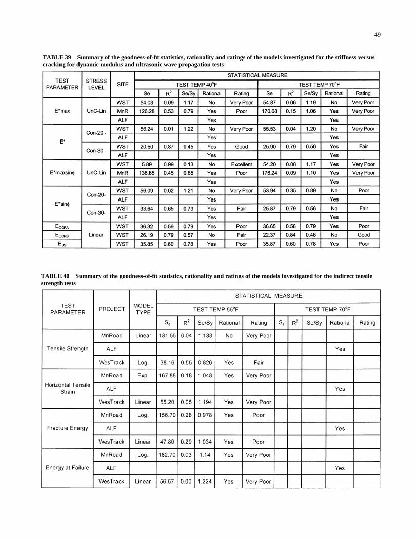
49
TABLE 39 Summary of the goodness-of-fit statistics, rationality and ratings of the models investigated for the stiffness versuscracking for dynamic modulus and ultrasonic wave propagation tests
TABLE 40 Summary of the goodness-of-fit statistics, rationality and ratings of the models investigated for the indirect tensilestrength tests
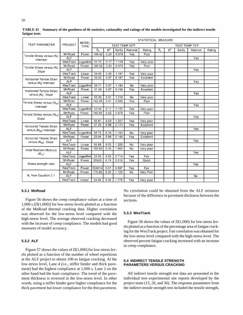
50
5.3.1 MnRoad
Figure 56 shows the creep compliance values at a time of1,000 s [D(1,000)] for low-stress levels plotted as a functionof the MnRoad thermal cracking data. Higher correlationwas observed for the low-stress level compared with thehigh-stress level. The average observed cracking decreasedwith the increase of creep compliance. The models had goodmeasures of model accuracy.
5.3.2 ALF
Figure 57 shows the values of D(1,000) for low-stress lev-els plotted as a function of the number of wheel repetitionsat the ALF project to obtain 100-m fatigue cracking. At thelow-stress level, Lane 4 (i.e., stiffer binder and thick pave-ment) had the highest compliance at 1,000 s. Lane 2 on theother hand had the least compliance. The trend of the pave-ment thickness is reversed in the low-stress level. In otherwords, using a stiffer binder gave higher compliance for thethick pavement but lower compliance for the thin pavement.
No correlation could be obtained from the ALF mixturesbecause of the difference in pavement thickness between thesections.
5.3.3 WesTrack
Figure 58 shows the values of D(1,000) for low-stress lev-els plotted as a function of the percentage area of fatigue crack-ing for the WesTrack project. Fair correlation was obtained forthe low-stress level compared with the high-stress level. Theobserved percent fatigue cracking increased with an increasein creep compliance.
5.4 INDIRECT TENSILE STRENGTHPARAMETERS VERSUS CRACKING
All indirect tensile strength test data are presented in theindividual test–experimental site reports developed by theproject team (15, 26, and 36). The response parameters fromthe indirect tensile strength test included the tensile strength,
TABLE 41 Summary of the goodness-of-fit statistics, rationality and ratings of the models investigated for the indirect tensilefatigue tests
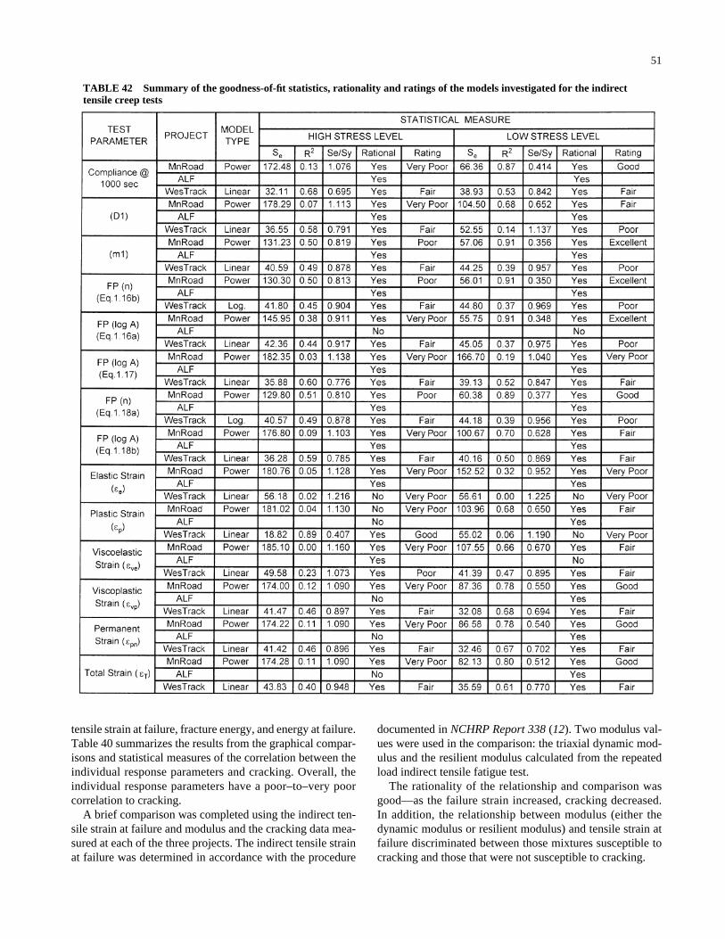
51
tensile strain at failure, fracture energy, and energy at failure.Table 40 summarizes the results from the graphical compar-isons and statistical measures of the correlation between theindividual response parameters and cracking. Overall, theindividual response parameters have a poor–to–very poorcorrelation to cracking.
A brief comparison was completed using the indirect ten-sile strain at failure and modulus and the cracking data mea-sured at each of the three projects. The indirect tensile strainat failure was determined in accordance with the procedure
documented in NCHRP Report 338 (12). Two modulus val-ues were used in the comparison: the triaxial dynamic mod-ulus and the resilient modulus calculated from the repeatedload indirect tensile fatigue test.
The rationality of the relationship and comparison wasgood—as the failure strain increased, cracking decreased.In addition, the relationship between modulus (either thedynamic modulus or resilient modulus) and tensile strain atfailure discriminated between those mixtures susceptible tocracking and those that were not susceptible to cracking.
TABLE 42 Summary of the goodness-of-fit statistics, rationality and ratings of the models investigated for the indirecttensile creep tests
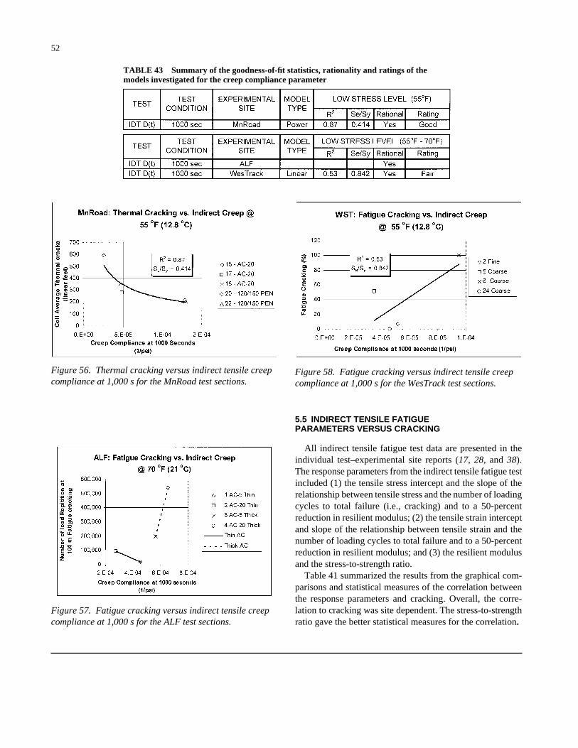
52
5.5 INDIRECT TENSILE FATIGUEPARAMETERS VERSUS CRACKING
All indirect tensile fatigue test data are presented in theindividual test–experimental site reports (17, 28, and 38).The response parameters from the indirect tensile fatigue testincluded (1) the tensile stress intercept and the slope of therelationship between tensile stress and the number of loadingcycles to total failure (i.e., cracking) and to a 50-percentreduction in resilient modulus; (2) the tensile strain interceptand slope of the relationship between tensile strain and thenumber of loading cycles to total failure and to a 50-percentreduction in resilient modulus; and (3) the resilient modulusand the stress-to-strength ratio.
Table 41 summarized the results from the graphical com-parisons and statistical measures of the correlation betweenthe response parameters and cracking. Overall, the corre-lation to cracking was site dependent. The stress-to-strengthratio gave the better statistical measures for the correlation.
Figure 56. Thermal cracking versus indirect tensile creepcompliance at 1,000 s for the MnRoad test sections.
Figure 57. Fatigue cracking versus indirect tensile creepcompliance at 1,000 s for the ALF test sections.
Figure 58. Fatigue cracking versus indirect tensile creepcompliance at 1,000 s for the WesTrack test sections.
TABLE 43 Summary of the goodness-of-fit statistics, rationality and ratings of themodels investigated for the creep compliance parameter
53
CHAPTER 6
SUMMARY OF FINDINGS
6.1 TEST METHODS APPLICABLE FOR THE SPT
Industry representatives were interviewed during the firstpart of Task C to determine which distress type was mostimportant in support of the Superpave volumetric mix designprocedure. Overwhelmingly, rutting (i.e., permanent defor-mation) was identified as the most important distress. As aresult, most follow-up work regarding the SPT was devoted todeveloping correlations between HMA mixture responseparameters and rutting. Fracture, however, also was consid-ered an important distress in the long-term performance ofHMA mixtures. As a result, the Superpave models team hascontinued to pursue the use of the SPT for analysis of fracture-related distresses, primarily load-related fatigue cracking.
There were specific requirements for developing the SPT:
• The SPT is to be used in support of the Superpave vol-umetric mix design procedure.
• The SPT must test HMA specimens compacted withSGC devices.
• The SPT must accurately measure true fundamentalresponses or properties of HMA mixtures, or both.
• The SPT must be based on existing technology andequipment (i.e., require no new test development).
• Responses measured with the SPT need not predict theentire performance history, but the test must identifyinferior HMA mixtures (i.e., must determine a mix’srelative susceptibility to excessive distortion and frac-ture under defined conditions).
• Properties determined from the SPT should be tied to theadvanced mixture characterization methods being devel-oped under other tasks of NCHRP Project 9-19, “Super-pave Support and Performance Models Management.”
Numerous test methods and mixture response parametersthat satisfy the above requirements were used in the experi-mental test plan for determining the correspondence betweenthe test results and the magnitude of rutting and cracking.Some of the test methods and equipment have been used fordecades for evaluating the performance characteristics ofHMA mixtures, while others have been recently developed.The following sections summarize the findings from the lab-oratory study and correlation to performance for the three
distresses considered (i.e., rutting, fatigue cracking, and ther-mal cracking).
6.1.1 SPT for Permanent Deformation—Rutting
Five laboratory tests consistently had parameters thatresulted in an overall good-to-excellent correlation to themeasured rut depths. These test methods and responses arethe dynamic modulus as measured by the SST and triaxialcompression tests at high temperatures, the flow time as mea-sured by the triaxial creep test, the cumulative permanentstrain measured at 1,000 loading cycles using the triaxialrepeated load test, and the permanent shear strain measuredat 1,000 loading cycles using the SST RSCH test.
6.1.1.1 Summary of Advantages andDisadvantages of Candidate Test Methods
Table 44 summarizes the advantages and disadvantagesfor each test method and response parameter found to behighly correlated to the amount of rutting. These advantagesand disadvantages were the consensus of the project teamand were based on the results of the testing program includedin this study and previous test programs. As shown, each testmethod has advantages and disadvantages regarding its usefor the SPT.
6.1.1.2 Ranking and Selection of Test Methodsand Responses
The purpose of the statistical analysis of all test data wasto find the best laboratory test method and parameter that sat-isfy the requirements of the SPT. The utility analysis sum-marized in Chapter 1 addressed several issues related to theselection process of the SPT. Some of these factors were asfollows:
• Reliability of the test parameter to distinguish amongthe performance of a wide range of mixtures,
• Repeatability of the test and the sensitivity of the testparameter to different mixture variables,

• Complexity of the test procedure,• Cost of the equipment and testing preparation require-
ments,• Testing time needed to complete the testing program,
and• Technical level or experience required from the operator.
Multiple members of the research team analyzed the statis-tical results, evaluated the potential test parameters, and out-lined the advantages and disadvantages of the test proceduresfor permanent deformation. The research team ranked thetests and parameters based on the comprehensive evaluationconducted on a scale from 1 to 6, 1 having the high or top pri-ority and 6 having the low or bottom. Results of the team’sevaluation and ranking procedure are shown in Table 45. Theoverall ranking for each test and parameter was obtained bytotaling the entire individual team ranking. The tests and para-meters then were ranked according to this sum. The lower thetotal score, the better the test.
54
As shown in Table 45, the top three parameters for per-manent deformation were (1) the dynamic modulus term,(E*/sinφ), determined from the triaxial dynamic modulustest; (2) the flow time (Ft) from the triaxial static creep; and(3) the flow number (Fn) from the triaxial repeated load test.During the July 2000 NCHRP panel meeting, the top twoparameters were recommended by the research team for thefollow-up field validation work. The panel’s recommenda-tion was to include the triaxial repeated load as a third alter-native. Thus, the above three test methods were selected asthe SPT candidates for evaluating an HMA mixture’s resis-tance to rutting.
6.1.2 SPT for Fracture—Fatigue and Thermal Cracking
Three laboratory tests had parameters that resulted in a faircorrelation to the measured amount of cracking. These test
TABLE 44 Advantages and disadvantages of the top-selected SPTs for permanent deformation
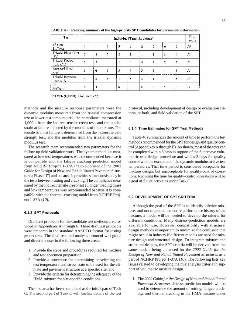
methods and the mixture response parameters were thedynamic modulus measured from the triaxial compressiontest at lower test temperatures, the compliance measured at1,000 s from the indirect tensile creep test, and the tensilestrain at failure adjusted by the modulus of the mixture. Thetensile strain at failure is determined from the indirect tensilestrength test, and the modulus from the triaxial dynamicmodulus test.
The research team recommended two parameters for thefollow-up field validation work. The dynamic modulus mea-sured at low test temperatures was recommended because itis compatible with the fatigue cracking–prediction modelfrom NCHRP Project 1-37A (“Development of the 2002Guide for Design of New and Rehabilitated Pavement Struc-tures: Phase II”) and because it provides some consistency inthe tests between rutting and cracking. The compliance mea-sured by the indirect tensile creep test at longer loading timesand low temperatures was recommended because it is com-patible with the thermal-cracking model from NCHRP Proj-ect 1-37A (10).
6.1.3 SPT Protocols
Draft test protocols for the candidate test methods are pro-vided in Appendixes A through E. These draft test protocolswere prepared in the standard AASHTO format for testingprocedures. The final test and analysis protocol will guideand direct the user in the following three areas:
1. Provide the steps and procedures required for mixtureand test specimen preparation,
2. Provide a procedure for determining or selecting thetest temperature and stress state to be used for the cli-mate and pavement structure at a specific site, and
3. Provide the criteria for determining the adequacy of theHMA mixture for site-specific conditions.
The first area has been completed as the initial part of TaskC. The second part of Task C will finalize details of the test
55
protocol, including development of design or evaluation cri-teria, or both, and field validation of the SPT.
6.1.4 Time Estimates for SPT Test Methods
Table 46 summarizes the amount of time to perform the testmethods recommended for the SPT for design and quality con-trol (Appendixes A through E). As shown, most of the tests canbe completed within 3 days in support of the Superpave volu-metric mix design procedure and within 2 days for qualitycontrol with the exception of the dynamic modulus at five testtemperatures. That time period is considered acceptable formixture design, but unacceptable for quality-control opera-tions. Reducing the time for quality-control operations will bea goal of future activities under Task C.
6.2 DEVELOPMENT OF SPT CRITERIA
Although the goal of the SPT is to identify inferior mix-tures and not to predict the entire performance history of themixture, a model will be needed to develop the criteria fordifferent conditions. Many distress-prediction models areavailable for use. However, compatibility with structuraldesign methods is important to minimize the confusion thatmight occur in industry if different models are used for mix-ture design and structural design. To integrate mixture andstructural designs, the SPT criteria will be derived from thesame models being enhanced for the 2002 Guide for theDesign of New and Rehabilitated Pavement Structures as apart of NCHRP Project 1-37A (10). The following lists keyissues related to developing the mix analysis criteria in sup-port of volumetric mixture design.
1. The 2002 Guide for the Design of New and RehabilitatedPavement Structures distress-prediction models will beused to determine the amount of rutting, fatigue crack-ing, and thermal cracking in the HMA mixture under
TABLE 45 Ranking summary of the high-priority SPT candidates for permanent deformation
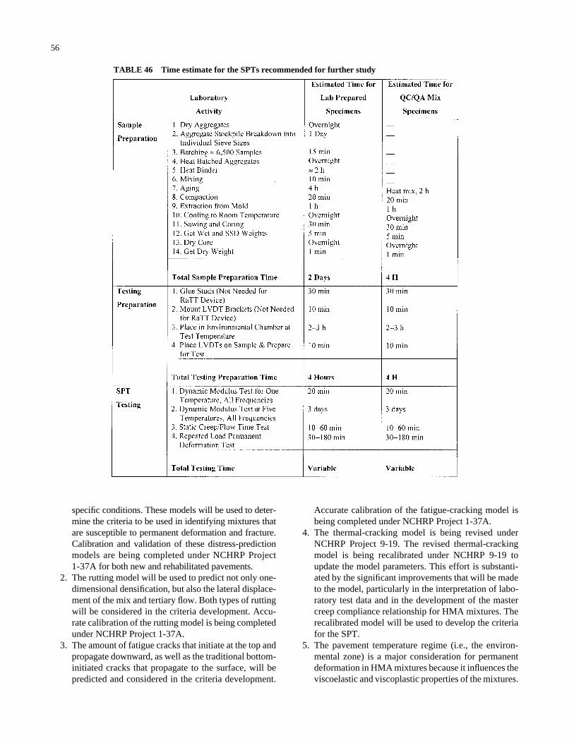
specific conditions. These models will be used to deter-mine the criteria to be used in identifying mixtures thatare susceptible to permanent deformation and fracture.Calibration and validation of these distress-predictionmodels are being completed under NCHRP Project 1-37A for both new and rehabilitated pavements.
2. The rutting model will be used to predict not only one-dimensional densification, but also the lateral displace-ment of the mix and tertiary flow. Both types of ruttingwill be considered in the criteria development. Accu-rate calibration of the rutting model is being completedunder NCHRP Project 1-37A.
3. The amount of fatigue cracks that initiate at the top andpropagate downward, as well as the traditional bottom-initiated cracks that propagate to the surface, will bepredicted and considered in the criteria development.
56
Accurate calibration of the fatigue-cracking model isbeing completed under NCHRP Project 1-37A.
4. The thermal-cracking model is being revised underNCHRP Project 9-19. The revised thermal-crackingmodel is being recalibrated under NCHRP 9-19 toupdate the model parameters. This effort is substanti-ated by the significant improvements that will be madeto the model, particularly in the interpretation of labo-ratory test data and in the development of the mastercreep compliance relationship for HMA mixtures. Therecalibrated model will be used to develop the criteriafor the SPT.
5. The pavement temperature regime (i.e., the environ-mental zone) is a major consideration for permanentdeformation in HMA mixtures because it influences theviscoelastic and viscoplastic properties of the mixtures.
TABLE 46 Time estimate for the SPTs recommended for further study
Temperature will be included as a key factor in devel-oping the criteria for permanent deformation and frac-ture. The temperature-equivalency concept will be usedto determine the test temperature for the SPT.
6. HMA layer thickness, insofar as it influences the mag-nitudes of stress and strain in the HMA layer, also hasrelevance to permanent deformation and fracture. Thetotal HMA layer thickness not only influences strainand stress magnitude, but is also linked to the locationwhere fatigue cracks initiate (i.e., at the bottom of theHMA layer or at the surface). Thus, total HMA thick-ness is considered a key factor in developing the eval-uation criteria.
7. Similar to the HMA layer thickness noted above, pave-ment type and rehabilitation strategy are additional fac-tors for checking the magnitudes of stress and strain inthe HMA mixture and failure hypothesis.
8. Traffic will be considered in the design criteria and willbe compatible with the Superpave mix design trafficcategories.
9. The modulus and strength of the supporting pavementlayers will be considered in the criteria development asthey related to the occurrence of fatigue cracks and, toa lesser extent, rutting.
6.3 FIELD VALIDATION OF THE SPT
The first major element of Task C was to select the best testmethods and responses for the SPT. The second major ele-ment of Task C is the field validation of the SPT and evalua-
57
tion criteria. The goal of most validation plans is to determinewhether (1) the conceptual model or test protocol is a reason-able representation of the real-world system and (2) thedesired accuracy exists between the laboratory (i.e., test pro-tocol) and the real-world system. In fact, the validation of theSPT is considered by industry to be the most important prod-uct of NCHRP Project 9-19.
NCHRP and the project team recognize that the long-termfield validation of the SPT protocol is critically important toits final acceptance and implementation in day-to-day Super-pave mix design practice. Thus, a field validation effort isneeded and planned for finalizing the test protocols and cri-teria. The goal of the field validation plan is to provide a reli-able, fully evaluated test protocol that can be used in supportof the Superpave volumetric design procedure.
One of the most time-consuming, expensive, and high-riskactivities associated with validating pavement-performancemodels is the collection of field performance data on a sub-stantial number of test sections. Field performance data is required for validating the SPT, Superpave mechanisticdistress-prediction models, the new 2002 Guide for the Designof New and Rehabilitated Pavement Structures (10) based onmechanistic–empirical principles, and other hypotheses for-mulated from the LTPP program.
Coordination of the data collection activities between proj-ects can substantially reduce the number of test sections thatwill be required if each project is conducted independently.Thus, the field validation plan for the SPT protocol and eval-uation criteria will use the LTPP SPS-9 experimental proj-ects and as many of the test sections as possible that are beingused on the other projects.
58
CHAPTER 7
RECOMMENDATIONS AND FUTURE ACTIVITIES
• HMA Low-Temperature Cracking (testing conductedat 0, −10, and −20°C):– The indirect tensile creep compliance, D(t), deter-
mined from the indirect tensile creep test.
Preliminary draft protocols for these SPTs are presented inthe appendixes to this report.
7.2 FUTURE ACTIVITIES
In the next phase of the project, the SPT method–responseparameter combinations shown in Section 7.1 will be furthervalidated using HMA materials and performance data from50 to 75 pavement sections in the FHWA LTPP SpecialPavement Study and similar full-scale field performanceexperiments. Based on these results, a final recommendationwill be made of SPT method-response parameter combina-tions to estimate the susceptibility of an HMA mix design torutting, fatigue cracking, and low-temperature cracking. Rec-ommendations will include proposed specification criteriadeveloped with the HMA performance models in the 2002Guide for the Design of New and Rehabilitated PavementStructures (10) and recommended test methods in AASHTOstandard format for future review and possible adoption bystate highway agencies.
In addition to the main field validation effort, four ancil-lary studies will be conducted toward the goals of simplify-ing the SPTs and making them as practical as possible. Thesestudies are briefly described in the following sections.
7.2.1 Specimen Diameter Study: 4-in. (100-mm)Versus 6-in. (150-mm)
A major cost in testing time and equipment expense arisesfrom the need to core and saw 4-in.-diameter SPT samplesfrom 6-in.-diameter gyratory-compacted specimens routinelymanufactured in the current Superpave mix design process.
This sample preparation was based on the conclusions of anextensive study on sample geometry and aggregate size con-ducted during NCHRP Project 9-19. It was found that (1) aminimum height-to-diameter ratio of 1.5 was required inorder to ensure that the response of a sample evaluated ineither the dynamic modulus or permanent deformation tests
7.1 SUMMARY AND RECOMMENDATIONS
This report presents the initial results of a comprehensiveresearch study to identify an SPT or a set of SPTs for use withthe Superpave volumetric mix design method. It describesthe selection of the best candidate simple performance testmethod–response parameter combinations through a detailedlaboratory evaluation of actual HMA materials obtained fromthree major U.S. accelerated pavement testing (APT) proj-ects: MnRoad, FHWA-ALF, and WesTrack.
The research assessed how well the measured results of33 combinations of SPTs and associated laboratory responseparameters correlated with the degree of distress observedwithin each experimental test section in the three APT proj-ects. Three major distress types were evaluated in this study.Rutting (i.e., permanent deformation) within the HMA layerwas present at all three field projects. Load-associated fatiguecracking was found at the ALF and WesTrack projects,although the fatigue experiment at the former project yieldedlimited results because of the small number of test sectionsused (i.e., two levels of thickness and two levels of asphaltconcrete stiffness–modulus). Transverse thermal fracture-associated low-temperature cracking only occurred at theMnRoad project. The actual effort expended by the researchteam for each distress was in relative proportion to the dis-tress’s generally acknowledged importance, that is, HMA rut-ting, load-associated fatigue fracture, and low-temperaturecracking, in that order.
The initial recommendations of the research team werereviewed by the NCHRP project panel, and the followingSPT method–response parameter combinations were selectedfor comprehensive field validation in the next phase of theproject.
• HMA Rutting (testing conducted at 100 to 130°F):– The dynamic complex modulus term, E*/sinφ, deter-
mined from the triaxial dynamic modulus test;– The flow time, Ft, determined from the triaxial static
creep test; and– The flow number, Fn, determined from the triaxial
repeated load test.• HMA Fatigue Cracking (testing conducted at 40 to
60°F):– The dynamic complex modulus, E*, determined from
the triaxial dynamic modulus test.
59
represents a fundamental engineering property; (2) a mini-mum sample diameter of 4 in. (100 mm) would be satisfac-tory for all HMA mixtures up to a maximum aggregate sizeof 1.5 in. (37.5 mm); and (3) smooth, parallel specimen endswere needed to eliminate end friction and violation of thetheoretical boundary effects of the specimen during the test.Another factor discouraging the use of the 6-in.-diameterspecimens is that numerous studies have illustrated the largedegree of nonhomogeniety of air voids within the largergyratory-compacted specimens. This variability, and its sub-sequent impact upon the variability of the SPT results, is sig-nificantly larger than the variability found when the smaller4-in.-diameter cored-and-sawn specimens are used.
This ancillary study will determine whether a constant mul-tiplier can be found between SPT results obtained on 4-in.-diameter and 6-in.-diameter specimens. Although the utilityof using the 4-in.-diameter specimen for the fundamentalresponse cannot be argued, it is also apparent that if an accu-rate common-multiplying factor can be determined for SPTsat differing diameters, the significant decrease in sample testtime and equipment cost over using the 4-in.-diameter cored-and-sawn specimens will be a major consideration in theeventual selection of the final SPT protocol.
7.2.2 Dynamic Complex Modulus Study:Flexural Versus Compressive Testing
All of the SPTs used for the rutting and load-associatedfatigue cracking distress are based on the use of 4-in.-diam-eter by 6-in.-high specimens tested in a uniaxial or triaxialcompressive mode. Although this specimen geometry is verycompatible with the use of gyratory-compacted specimens involumetric mix design, it does present problems if the SPTsare used for forensic investigations of existing pavements,either to prepare for the rehabilitation or to identify specificcauses of premature distress. Generally, pavements do notincorporate single, 6-in.-high HMA layers, so obtaining aspecimen with the appropriate height-to-diameter ratio forthe SPT is nearly impossible.
This ancillary study will investigate whether the dynamiccomplex modulus measured in compression on 4-in.-diameterby 6-in.-high specimens can be correlated to the modulus val-ues measured from flexural beam stiffness testing. If a true
equivalence between the two tests exists, beam testing can beused with the appropriate SPT specification criteria to esti-mate the performance characteristics of the existing HMApavement.
7.2.3 Sensitivity Study: SPT ResponseParameter and Magnitude
This ancillary study will investigate the sensitivity of can-didate SPT response parameters to key HMA mixture prop-erties. For example, if the SPT response parameter chosen tomeasure HMA rutting does not significantly change as a func-tion of the amount of asphalt cement in the mix, the accuracyof the SPT as an indicator of performance and distress will besuspect.
The study will focus on the sensitivity of the SPT responseparameter as a function of the air voids and asphalt binder con-tents (Va and Vb) in both confined and unconfined testing. If timeand resources allow, the sensitivity of the response parametersto other mix variables such as asphalt-binder type, aggregategradation, and aggregate type will also be investigated.
7.2.4 Tertiary Flow Measurement Methods Study
The SPTs based on the triaxial repeated load and triaxialstatic creep tests use the point of initiation of tertiary flow inthe HMA mixture to determine its flow number (Fn ) and flowtime (Ft ), respectively. The tertiary phase is easily distin-guishable from the secondary phase in both the repeatedloading and static creep tests by comparing the first deriva-tives (i.e., rates of change) of the test-response parameters.These deformation measurements commonly use vertical-mounted LVDTs to measure the deformation of the test spec-imens under load. However, there is some evidence that iden-tical flow numbers and times can be generated by assessingthe rate response of radial-mounted LVDTs.
This ancillary study will investigate the feasibility of defin-ing the flow time, flow number, or both, of an HMA mixturefrom measurements made with radial LVDTs and the loadram actuator as well as with vertical LVDTs. The purpose isto find the simplest practical way to determine the flow timeand flow number with the respective SPTs.
60
REFERENCES
1. Leahy, R.B., E.T. Harrigan, and H. Von Quintus. Validation ofRelationships Between Specification Properties and Perfor-mance. Report No. SHRP-A-409. Transportation ResearchBoard, National Research Council, Washington, DC (1994).
2. Mix Design Methods for Asphalt Concrete and Other Hot-MixTypes. 6th edition. The Asphalt Institute, Lexington, KY (1997).
3. “Preliminary Recommendations for the Simple PerformanceTest,” Interim Task C Report, FHWA Contract DTFH61-95-C-00100. University of Maryland, College Park, MD (1998).
4. Cominsky, R.J., B.M. Killingsworth, R.M. Anderson, D.A.Anderson, and W.M. Crockford. NCHRP Report 409: QualityControl and Acceptance of Superpave-Designed Hot MixAsphalt. Transportation Research Board, National ResearchCouncil, Washington, DC (1998).
5. Witczak, M.W., D. Andrei, and W. Mirza. “Development ofRevised Predictive Model for the Dynamic (Complex) Modu-lus of Asphalt Mixtures,” Interteam Technical Report, NCHRPProject 1-37A, University of Maryland, March 1999.
6. Bonnaure, F., G. Gest, A. Garvois, and P. Uge. “A New Methodof Predicting the Stiffness of Asphalt Paving Mixes,” Journalof the Association of Asphalt Paving Technologists, Vol. 46(1977).
7. Drucker, D.C. “Limit Analysis of Two- and Three-Dimen-sional Soil Mechanics Problems,” Journal of Mechanics andPhysical Solids, Vol. 1 (1953).
8. Hafez, I. “Development of a Simplified Asphalt Mix StabilityProcedure for Use in Superpave Volumetric Mix Design.”Ph.D. Dissertation, Civil Engineering Department, Universityof Maryland, College Park, MD (1997).
9. Witczak, M.W., M.W. Mirza, and K. Kaloush. “ComplianceModel Development,” NCHRP Project 1-37A Interim ReportUniversity of Maryland, College Park, MD (1997).
10. ERES Consultants, Inc. “Development of 2002 Guide for theDesign of New and Rehabilitated Pavement Structures—StageA Report,” NCHRP Project 1-37A Interim Report (1999).
11. ERES Consultants, Inc. “LTPP Data Analysis Technical Assis-tance,” FHWA Contract DTFH61-96-C-00003, Washington,DC (2002).
12. Von Quintus, H.L., J.A. Scherocman, C.S. Hughes, and T.W.Kennedy. NCHRP Report 338: Asphalt-Aggregate MixtureAnalysis System: AAMAS. Transportation Research Board,National Research Council, Washington, DC (1991).
13. Witczak, M.W., and M.W. Mirza. “Development of Relation-ships to Predict Poisson’s Ratio for Paving Materials,”Interteam Technical Report for NCHRP 1-37A. University ofMaryland, College Park, MD (1999).
14. Roque, R., R.L. Lytton, J. Uzan, E.G. Fernando, D. Hiltunen,and S.M. Stoffels. Development and Validation of Perfor-mance Prediction Models and Specifications for AsphaltBinders and Paving Mixes. Report No. SHRP-A-357, Trans-portation Research Board, National Research Council, Wash-ington, DC (1993).
15. Witczak, M.W., M. El-Basyouny, and M.W. Mirza. “IndirectTensile Strength Test,” NCHRP Project 9-19, Task C. TeamReport SPT-MN-2(A) (MnRoad Experiment), Arizona StateUniversity, Tempe, AZ (1999).
16. Witczak, M.W., M. El-Basyouny, and M.W. Mirza. “IndirectCreep Test,” Team NCHRP Project 9-19, Task C. Report SPT-MN-2(B) (MnRoad Experiment), Arizona State University,Tempe, AZ (1999).
17. Witczak, M.W., M. El-Basyouny, and M.W. Mirza. “IndirectFatigue Tests,” NCHRP Project 9-19, Task C. Team ReportSPT-MN-2(C) (MnRoad Experiment), Arizona State Univer-sity, Tempe, AZ (1999).
18. Witczak, M.W., S.H. Cardoso, and K. Kaloush. “TriaxialStrength Test,” NCHRP Project 9-19, Task C. Team ReportSPT-MN-2(D) (MnRoad Experiment), Arizona State Univer-sity, Tempe, AZ (1999).
19. Witczak, M.W., S.H. Cardoso, and T. Pellinen. “G*-FieldShear Test (FST),” NCHRP Project 9-19, Task C. Team ReportSPT-MN-2(E) (MnRoad Experiment), Arizona State Univer-sity, Tempe, AZ (1999).
20. Witczak, M.W., R. Bonaquist. “G*-Simple Shear Tests (SST),”NCHRP Project 9-19, Task C. Team Report SPT-MN-2(F)(MnRoad Experiment), Arizona State University, Tempe, AZ(1999).
21. Witczak, M.W., G. Huber, and X. Zhang. “Repeated Shear Per-manent Deformation Tests,” NCHRP Project 9-19, Task C.Team Report SPT-MN-2(G) (MnRoad Experiment), ArizonaState University, Tempe, AZ (1999).
22. Witczak, M.W., and K. Kaloush. “Repeated Normal PermanentDeformation Tests,” NCHRP Project 9-19, Task C. TeamReport SPT-MN-2(H) (MnRoad Experiment), Arizona StateUniversity, Tempe, AZ (1999).
23. Witczak, M.W., and K. Kaloush. “Triaxial Static Creep Test(Flow and Compliance),” NCHRP Project 9-19, Task C. TeamReport SPT-MN-2(I) (MnRoad Experiment), Arizona StateUniversity, Tempe, AZ (1999).
24. Witczak, M.W., and T. Pellinen. “E*-Dynamic Complex Mod-ulus and Ed-Dynamic Pulse Wave Velocity Tests,” NCHRPProject 9-19, Task C. Team Report SPT-MN-2(J-K) (MnRoadExperiment), Arizona State University, Tempe, AZ (1999).
25. Witczak, M.W., T. Pellinen, and D. Andrei. “E* and Sm Pre-diction Equation Methodology Results,” NCHRP Project 9-19,Task C. Team Report SPT-MN-2(L) (MnRoad Experiment),Arizona State University, Tempe, AZ (1999).
26. Witczak, M.W., M. El-Basyouny, and M.W. Mirza. “IndirectTensile Strength Test,” NCHRP Project 9-19, Task C. TeamReport SPT-ALF-2(A) (ALF Experiment), Arizona State Uni-versity, Tempe, AZ (2000).
27. Witczak, M.W., M. El-Basyouny, and M.W. Mirza. “IndirectCreep Test,” NCHRP Project 9-19, Task C. Team Report SPT-ALF-2(B) (ALF Experiment), Arizona State University,Tempe, AZ (2000).
28. Witczak, M.W., M. El-Basyouny, and M.W. Mirza. “IndirectFatigue Tests,” NCHRP Project 9-19, Task C. SPT-ALF-2(C)(ALF Experiment), Arizona State University, Tempe, AZ(2000).
29. Witczak, M.W., Cardoso, S.H., and K. Kaloush. “TriaxialStrength Test,” NCHRP Project 9-19, Task C. Team ReportSPT-ALF-2(D) (ALF Experiment), Arizona State University,Tempe, AZ (2000).
61
30. Witczak, M.W., and R. Bonaquist. “G*-Simple Shear Tests(SST),” NCHRP Project 9-19, Task C. Team Report SPT-ALF-2(F) (ALF Experiment), Arizona State University, Tempe, AZ(2000).
31. Witczak, M.W., G. Huber, and X. Zhang. “Repeated Shear Per-manent Deformation Tests,” NCHRP Project 9-19, Task C.Team Report SPT-ALF-2(G) (ALF Experiment), Arizona StateUniversity, Tempe, AZ (2000).
32. Witczak, M.W., and K. Kaloush. “Repeated Normal PermanentDeformation Tests,” NCHRP Project 9-19, Task C. TeamReport SPT-ALF-2(H) (ALF Experiment), Arizona State Uni-versity, Tempe, AZ (2000).
33. Witczak, M.W., and K. Kaloush. “Triaxial Static Creep Test(Flow and Compliance),” NCHRP Project 9-19, Task C. TeamReport SPT-ALF-2(I) (ALF Experiment), Arizona State Uni-versity, Tempe, AZ (2000).
34. Witczak, M.W., and T. Pellinen. “E*-Dynamic Complex Mod-ulus and Ed-Dynamic Pulse Wave Velocity Tests,” NCHRPProject 9-19, Task C. Team Report SPT-ALF-2(J-K) (ALFExperiment), Arizona State University, Tempe, AZ (2000).
35. Witczak, M.W., and T. Pellinen. “E* and Sm Prediction Equa-tion Methodology Results,” NCHRP Project 9-19, Task C.Team Report SPT-ALF-2(L) (ALF Experiment), Arizona StateUniversity, Tempe, AZ (2000).
36. Witczak, M.W., M. El-Basyouny, and M.W. Mirza, “IndirectTensile Strength Test,” NCHRP Project 9-19, Task C. TeamReport SPT-WST-2(A) (WesTrack Experiment), Arizona StateUniversity, Tempe, AZ (2000).
37. Witczak, M.W., M. El-Basyouny, and M.W. Mirza. “IndirectCreep Test,” NCHRP Project 9-19, Task C. Team Report SPT-WST-2(B) (WesTrack Experiment), Arizona State University,Tempe, AZ (2000).
38. Witczak, M.W., M. El-Basyouny, and M.W. Mirza. “IndirectFatigue Tests,” NCHRP Project 9-19, Task C. Team ReportSPT-WST-2(C) (WesTrack Experiment), Arizona State Uni-versity, Tempe, AZ (2000).
39. Witczak, M.W., S.H. Cardoso, and K. Kaloush. “TriaxialStrength Test,” NCHRP Project 9-19, Task C. Team Report
SPT-WST-2(D) (WesTrack Experiment), Arizona State Uni-versity, Tempe, AZ (2000).
40. Witczak, M.W., R. Bonaquist “G*-Simple Shear Tests (SST),”NCHRP Project 9-19, Task C. Team Report SPT-WST-2(F)(WesTrack Experiment), Arizona State University, Tempe, AZ(2000).
41. Witczak M.W., G. Huber, and X. Zhang. “Repeated Shear Per-manent Deformation Tests,” NCHRP Project 9-19, Task C.Team Report SPT-WST-2(G) (WesTrack Experiment), Ari-zona State University, Tempe, AZ (2000).
42. Witczak, M.W., and K. Kaloush. “Repeated Normal PermanentDeformation Tests,” NCHRP Project 9-19, Task C. TeamReport SPT-WST-2(H) (WesTrack Experiment), Arizona StateUniversity, Tempe, AZ (2000).
43. Witczak, M.W., and K. Kaloush. “Triaxial Static Creep Test(Flow and Compliance),” NCHRP Project 9-19, Task C. TeamReport SPT-WST-2(I) (WesTrack Experiment), Arizona StateUniversity, Tempe, AZ (2000).
44. Witczak, M.W., and T. Pellinen. “E*-Dynamic Complex Mod-ulus and Ed-Dynamic Pulse Wave Velocity Tests,” NCHRPProject 9-19, Task C. Team Report SPT-WST-2(J-K) (Wes-Track Experiment), Arizona State University, Tempe, AZ(2000).
45. Witczak, M.W., and T. Pellinen. “E* and Sm Prediction Equa-tion Methodology Results,” NCHRP Project 9-19, Task C.Team Report SPT-MN-2(L) (WesTrack Experiment), ArizonaState University, Tempe, AZ (2000).
46. Method for Preparation of Triaxial Specimens (Test ProtocolUMD 9808), “Superpave Models Team Inter-Laboratory Test-ing Manual.” University of Maryland, College Park, MD(1998).
47. Witczak, M.W., R. Bonaquist, H. Von Quintus, and K.Kaloush. “Specimen Geometry and Aggregate Size Lab TestStudy,” NCHRP Project 9-19, Task C. Team Report SLS-3,Arizona State University, Tempe, AZ (1999).
48. Azari, H., M.W. Witczak, and W. Mirza. “Development of Pre-dictive Model for Asphalt Concrete Phase Angle,” InterteamTechnical Report, NCHRP Project 1-37A, University of Mary-land, April 1999.

62
GLOSSARY
ABBREVIATIONS
AC = asphalt concreteALF = accelerated loading facility, Turner–FairbanksAPT = accelerated pavement testing
F or FC = fatigue cracking FSCH = frequency sweep at constant height test
FST = field shear testerHMA = hot mix asphalt
IDT = indirect tensileLTPP = long-term pavement performance
LVDT = linear variable differential transducerMESAL = million equivalent single axle load
PG = performance gradeQC = quality control
R = rutting or rut depthRSCH = repeated shear at constant height test
SGC = Superpave gyratory compactorSHRP = Strategic Highway Research Program
SPT = simple performance testSSCH = simple shear at constant height test
SSD = surface saturated dry test methodSST = Superpave shear tester
T or TC = thermal cracking
NOTATIONS
a = intercepta, b = mixture permanent deformation parameters,
regression coefficients from the secondary por-tion of the cumulative permanent deformationcurve
a, m = materials regression coefficients from the visco-elastic compliance function
a, b, d, = integration constants for the indirect tensile testthat are specimen geometry dependent
b = slope
c = cohesion or intercept parameter from a triaxialshear strength test
d = diameter of the test specimenD = densityD′ = viscoelastic compliance component at any timeDo = instantaneous compliance
D(t) = total compliance at any timeD1, m1 = mixture compliance parameters or regression
coefficients from an indirect tensile creep test
E = modulus of elasticity or Young’s modulusE* = complex modulus
|E*| = dynamic modulusE′ = storage or elastic modulusE″ = loss or viscous modulusEd = elastic modulusER = resilient modulus
f = loading frequencyFn = flow number from a repeated load permanent defor-
mation testFt = flow time from a static creep test
g = 32.19 ft/s2
G* = shear complex modulus|G*| = shear dynamic modulus
G′ = shear storage modulusG″ = shear loss or viscous modulus
i = imaginary unit from the complex modulus testI1 = first invariant stress tensor
J2 = second invariant deviatoric stress tensor
k = intercept parameter of the Drucker–Prager failureenvelope
K1, K2 = regression coefficients or constants from a repeatedload fatigue test
L = distance between the transducers for an ultrasonicwave propagation test
m = slope
n = sample size or number of test specimensN = number of loading cycles
Nf = number of loading cycles to failure, fracture lifeN50 = number of loading cycles to a 50 percent reduction
in the modulus of a test specimen during a fatiguetest
P = applied load
R2 = coefficient of determination
St = indirect tensile strengthSe = standard errorSy = standard deviation of the criterion variableSb = binder modulus for the Shell Oil predictive equation

63
Sm = HMA mixture modulus from the Shell Oil predic-tive equation
t = thickness of the test speciment = timeti = time lag between a cycle of stress and straintp = time for a stress cycle T = effective transit time for an ultrasonic wave propa-
gation test
V = pulse velocity from an ultrasonic wave propagationtest
Va = air void content in HMA mixtures, %Vb = volume of bitumen
Vbeff = effective bitumen content, % by volumeVg = volume of aggregate
α, µ = plastic or permanent deformation parameters from arepeated load test
β1–β4 = regression constants in the Shell Oil predictive equa-tion
δXX = horizontal deformation across the test specimenfrom an indirect tensile test
ε = normal strainεe = elastic strain, recoverable and time-independentεo = recoverable axial strainεp = cumulative permanent or plastic strain, irrecoverable
and time-independentεr = resilient or recoverable axial strainεT = total strainεve = viscoelastic strain, recoverable and time-dependentεvp = viscoplastic strain, irrecoverable and time-dependentεxx = horizontal tensile strain in an indirect tensile test
specimen
εff = horizontal tensile strain at failure from an indirecttensile test
Γfr = total fracture energyΓfa = fracture energy to failure
η = bitumen viscosity
ρ = densityρ4 = cumulative percentage retained on 4.76-mm sieve
ρ34 = cumulative percentage retained on 19-mm sieveρ38 = cumulative percentage retained on 9.5-mm sieve
ρ200 = percentage passing the 0.075-mm sieve
φ = slope of the failure envelope or the angle of internalfriction from a triaxial shear strength test
φ = phase angle from the complex modulus test
γ = slope of the Drucker–Prager failure envelopeγ = shear strain
γo = peak shear strain amplitudeγp = plastic shear strainγr = resilient or recoverable shear strain
σo = dynamic stressσ = normal stress
σxx = horizontal tensile stress in an indirect tensile test spec-imen
τ = shear stressτo = peak shear stress amplitude
µ = Poisson’s ratio
ν = number of regression coefficientsνcl = velocity of sound
64
APPENDIX A
TEST METHOD FOR DYNAMIC MODULUS OF ASPHALT CONCRETE MIXTURESFOR PERMANENT DEFORMATION
1. Scope
1.1 This test method covers procedures for preparing andtesting asphalt concrete mixtures to determine thedynamic modulus and phase angle at a single effectivetemperature Teff and design loading frequency.
1.2 This test method is a part of test protocols that includedetermination of the dynamic modulus of the asphaltmix for paving purposes. The other test methods areStandard Test Method for Simple Performance Test forFatigue Cracking based Upon Dynamic Modulus ofAsphalt Concrete Mixture and Standard Test Methodfor Dynamic Modulus of Asphalt Concrete Mixtures,which is for constructing a master curve for character-izing asphalt concrete for pavement thickness designand performance analysis.
1.3 This standard is applicable to laboratory-prepared spec-imens of mixtures with nominal maximum size aggre-gate less than or equal to 37.5 mm (1.5 in).
1.4 This standard may involve hazardous material, oper-ations, and equipment. This standard does not pur-port to address all safety problems associated with itsuse. It is the responsibility of the user of this proce-dure to establish appropriate safety and health prac-tices and to determine the applicability of regulatorylimitations prior to use.
2. Referenced Documents
2.1 AASHTO Standards
TP4 Method for Preparing and Determining theDensity of Hot Mix Asphalt (HMA) Spec-imens by Means of the SHRP GyratoryCompactor
PP2 Practice for Mixture Conditioning of HotMix Asphalt (HMA)
T67 Standard Practices for Load Verificationof Testing Machines (cross-listed withASTM E4)
T269 Percent Air Voids in Compacted Dense andOpen Bituminous Paving Mixtures
3. Definitions
3.1 Dynamic Modulus—|E*|, the norm value of the com-plex modulus calculated by dividing the peak-to-peak
stress by the peak-to-peak strain for a material sub-jected to a sinusoidal loading.
3.2 Complex Modulus—E*, a complex number that definesthe relationship between stress and strain for a linearviscoelastic material.
3.3 Phase angle—∂, the angle in degrees between a sinu-soidally applied stress and the resulting strain in acontrolled-stress test.
3.4 Linear viscoelastic—within the context of this test,refers to behavior in which the dynamic modulus isindependent of stress or strain amplitude.
3.5 Effective Temperature Teff—Is a single test tempera-ture at which an amount of permanent deformationwould occur equivalent to that measured by consider-ing each season separately throughout the year.
4. Summary of Method
4.1 A sinusoidal (haversine) axial compressive stress isapplied to a specimen of asphalt concrete at a giventemperature and loading frequency. The applied stressand the resulting recoverable axial strain response ofthe specimen is measured and used to calculate thedynamic modulus and phase angle.
4.2 Figure 1 presents a schematic of the dynamic modu-lus test device.
5. Significance and Use
5.1 Dynamic modulus values, measured at one effectivetemperature Teff and one design frequency selected bythe design engineer, are used as performance criteriafor permanent deformation resistance of the asphaltconcrete mixture to be used in conjunction with theSuperpave Volumetric Mix Design Method.
Note 1—The effective temperature Teff coversapproximately the temperature range of 25 to 60°C(77 to 140°F).
Note 2—10 Hz frequency can be used for highwayspeed and 0.1 Hz for creep—intersection traffic.
5.2 Dynamic modulus values measured over a range oftemperatures and frequencies of loading can be shifted
into a master curve for characterizing asphalt con-crete for pavement thickness design and performanceanalysis.
5.3 This test method covers the determination of thedynamic modulus values measured unconfined withinthe linear viscoelastic range of the asphalt mixture.
Note 3—Future research may indicate the need forconfined stress states and nonlinear material char-acterization. Confinement may be applied with var-ious types of axisymmetric triaxial cells to addressthese needs.
6. Apparatus
6.1 Dynamic Modulus Test System—A dynamic modu-lus test system consisting of a testing machine, envi-ronmental chamber, measuring system, and specimenend fixtures.
6.1.1 Testing Machine—A materials testing machinecapable of producing a controlled haversine com-pressive loading of paragraphs 9.7 and 9.8 isrequired.
Note 4—The testing machine shall have a capabil-ity of applying load over a range of frequenciesfrom 0.1 to 30 Hz. Stress levels up to 2800 kPa(400 psi) may be required at certain temperaturesand frequencies. However, for virtually all effec-tive temperatures in the US, stress levels between10 kPa and 690 kPa (1.5–100 psi) have been foundto be sufficient. This latter range of stress levelsconverts to an approximate range of 0.08–5.5 kN18–1218 lbf) on a 100 mm diameter specimen. Ifthe machine is to be dedicated only to this test pro-cedure with no requirement for additional strengthtesting or low temperature testing, it is recom-mended that the lowest capacity machine capableof applying the required waveforms be used. Alter-natively, larger capacity machines may be usedwith low capacity load cells or signal amplifiers. Ithas been found that feedback controlled testingmachines equipped with appropriate servovalvescan be used for this test. As a general rule of thumb,the dynamic load capacity of a testing machinebetween 10 and 30 Hz will be approximately 65–75percent of the monotonic (“static”) capacity, butthis rule varies by manufacturer. A 25–50 kN capac-ity servohydraulic testing machine has been foundto be adequate for virtually all of the tests in thesuite of simple performance tests.
6.1.2 Environmental Chamber—A chamber for con-trolling the test specimen at the desired tempera-
65
ture is required. The environmental chamber shallbe capable of controlling the temperature of thespecimen over a temperature range from 25 to60°C (77 to 140°F ) to an accuracy of ±0.5°C(1°F). The chamber shall be large enough toaccommodate the test specimen and a dummyspecimen with temperature sensor mounted at thecenter for temperature verification.
Note 5—A chamber that will control temperaturesdown to −10°C (14°F) may be required for othertests mentioned in paragraph 1.2 of this method.
Note 6—If the chamber does not have sufficientroom for a dummy specimen, it is permissible tohave a second chamber controlling the temperatureof the dummy. The separate dummy chamber mustbe operated similar to the operation of the main testspecimen chamber so that the dummy will accu-rately register the time required to obtain tempera-ture equilibrium on the test specimen.
6.1.3 Measurement System—The system shall includea data acquisition system comprising analog todigital conversion and/or digital input for storageand analysis on a computer. The system shall becapable of measuring and recording the time his-tory of the applied load and the axial deforma-tions for the cycles required by this test method.The system shall be capable of measuring theperiod of the applied sinusoidal load and result-ing deformations with a resolution of 0.5 percent.
6.1.3.1 Load—The load shall be measured with anelectronic load cell having adequate capacityfor the anticipated load requirements. Theload cell shall be calibrated in accordancewith AASHTO T67. The load measuringtransducer shall have an accuracy equal to orbetter than 0.25 percent of full scale.
Note 7—A 25 kN (5600 lbf) load cell has beenfound to be the approximate maximum capacitylimit for this test method because of range versusresolution factors. It is recommended that if theselected load cell capacity is 25 kN or greater, thesystem should be equipped with either manual orautomatic amplification selection capability so thatit can be used to enhance control of the system at theminimum anticipated loads given in paragraph 9.7.
Axial Deformations—Axial deformations shall be measuredwith displacement transducers referenced to gauge pointscontacting the specimen as shown in Figure 2. The deforma-tions shall be measured at a minimum of two locations 180°
66
apart (in planview); however, three locations located 120°apart is recommended to minimize the number of replicatespecimens required for testing.
Note 8—Analog transducers such as linear vari-able differential transformers (LVDTs) having arange of ±0.5 mm (0.02 in) and inherent nonlin-earity equal to or better than ±0.025 percent of fullscale have been found adequate for this purpose.Software or firmware linearization techniques maybe used to improve the inherent nonlinearity.Amplification and signal conditioning techniquesmay be used with the ±0.5 mm range LVDTs toobtain resolutions down to 0.001mm (0.00004 in)or better for small strain tests conditions. Thesetechniques may be manual or automatic. In gen-eral, increasing the resolution by manual signalamplification will result in reduction of the overallrange of the instrument by the same factor.
6.1.4 Loading Platens—Platens, with a diameter equalto or greater than that of the test specimen arerequired above and below the specimen to trans-fer the load from the testing machine to the spec-imen. Generally, these platens should be madeof anodized high strength aluminum. Softer mate-rials will require more frequent replacement.Materials that have linear elastic modulus proper-ties and hardness properties lower than that of6061-T6 aluminum shall not be used. Steel platensmay cause too much seating load to the specimenat high temperature and are not recommended.
6.1.5 End Treatment—Friction reducing end treatmentsshall be placed between the specimen ends andthe loading platens.
Note 9—End treatments consisting of two 0.5 mm(0.02 in) thick latex sheets separated with siliconegrease have been found to be suitable friction reduc-ing end treatments.
6.2 Gyratory Compactor—A gyratory compactor andassociated equipment for preparing laboratory speci-mens in accordance with AASHTO TP4 shall be used.Field cores shall meet the requirements of paragraphs7.4 through 7.6 of this test method and any reportson cores so tested will contain a detailed descriptionof the location of any lift boundaries within the heightof the specimen (e.g. lift order, thickness and materialhomogeneity).
6.3 Saw—A machine for cutting test specimens to theappropriate length is required. The saw or grindingmachine shall be capable of cutting specimens to the
prescribed dimensions without excessive heating orshock.
Note 10—A double-bladed diamond masonry sawgreatly facilitates the preparation of test specimenswith smooth, parallel ends. Both single- and double-bladed diamond saws should have feed mecha-nisms and speed controls of sufficient precision toensure compliance with paragraphs 7.5 and 7.6 ofthis method. Adequate blade stiffness is also impor-tant to control flexing of the blade during thin cuts.
6.4 Core Drill—A coring machine with cooling systemand a diamond bit for cutting nominal 100 mm (4 in)diameter test specimens.
Note 11—A coring machine with adjustable verti-cal feed and rotational speed is recommended. Thevariable feeds and speeds may be controlled by var-ious methods. A vertical feed rate of approximately0.05 mm/rev (0.002 in/rev) and a rotational speedof approximately 455 RPM has been found to besatisfactory for several of the Superpave mixtures.
7. Test Specimens
7.1 Size—Dynamic modulus testing shall be performedon 100 mm (4 in) diameter by 150 mm (6 in) high testspecimens cored from gyratory compacted mixtures.
7.2 Aging—Mixtures shall be aged in accordance with theshort-term oven aging procedure in AASHTO PP2.
7.3 Gyratory Specimens—Prepare 165 mm (6.5 in) highspecimens to the required air void content in accor-dance with AASHTO TP-4.
Note 12—Testing should be performed on test spec-imens meeting specific air void tolerances. Thegyratory specimen air void content required toobtain a specified test specimen air void contentmust be determined by trial and error. Generally,the test specimen air void content is 1.5 to 2.5 per-cent lower than the air void content of the gyratoryspecimen when the test specimen is removed fromthe middle as specified in this test method.
7.4 Coring—Core the nominal 100 mm (4 in) diametertest specimens from the center of the gyratory speci-mens. Both the core drill and the gyratory specimenshould be adequately supported to ensure that theresulting test specimen is cylindrical with sides thatare smooth, parallel, and free from steps, ridges, andgrooves.
7.5 Diameter—Measure the diameter of the test specimenat the mid-height and third points along axes that are
67
presents details of the mounting studs and LVDTmounting hardware.
Note 14—Quick setting epoxy such as Duro Mas-ter Mend Extra Strength Quick Set QM-50 has beenfound satisfactory for attaching studs. Under cer-tain conditions when using the triaxial cell men-tioned in Note 3, the mounting studs may notrequire gluing to the specimen. While the surfacecontact area of the mounting studs is normally min-imized consistent with transducer support require-ments, it is generally recommended that the area ofthe studs be sufficiently large to bridge any openvoid structure features evident on the cut face ofthe specimen. The minimum diameter mountingstud consistent with support requirements is nor-mally set at 8 mm (0.315 in), maximum diametershave not been established. A circular stud contactsurface shape is not required, rectangular or othershapes are acceptable.
8.2 The gauge length for measuring axial deformationsshall be 100 mm ±1 mm. An alignment and spacingfixture similar to that shown in Figure 3 can be usedto facilitate mounting of the axial deformation mea-suring hardware. The gauge length is normally mea-sured between the stud centers.
9. Procedure
9.1 The recommended test protocol for the Simple Perfor-mance Test for use in the Superpave volumetric mixdesign consists of testing the asphalt mix at one effec-tive pavement temperature Teff and one design frequencyselected by the design engineer. The effective pavementtemperature Teff covers approximately the temperaturerange of 25 to 60°C (77 to 140°F). The design frequencycovers the range between 0.1 to 10 Hz.
9.2 Place the test specimen in the environmental cham-ber and allow it to equilibrate to the specified testingtemperature. A dummy specimen with a temperaturesensor mounted at the center can be monitored todetermine when the specimen reaches the specifiedtest temperature. In the absence of the dummy speci-men, Table 2 summarizes minimum recommendedtemperature equilibrium times from room temperature(i.e. 25°C).
9.3 Place one of the friction reducing end treatments ontop of the platen at the bottom of the loading frame.Place the specimen on top of the lower end treatment,and mount the axial LVDTs to the hardware previ-ously attached to the specimen. Adjust the LVDT to
90 degrees apart. Record each of the six measurementsto the nearest 1 mm (0.05 in). Calculate the averageand the standard deviation of the six measurements. Ifthe standard deviation is greater than 2.5 mm (0.01 in)discard the specimen. For acceptable specimens, theaverage diameter, reported to the nearest 1 mm, shallbe used in the stress calculations.
7.6 End Preparation—The ends of all test specimens shallbe smooth and perpendicular to the axis of the speci-men. Prepare the ends of the specimen by sawing witha single- or double-bladed saw. The prepared speci-men ends shall meet the tolerances described below.Reject test specimens not meeting these tolerances.
7.6.1 The specimen ends shall have a cut surface wavi-ness height within a tolerance of ±0.05 mm acrossany diameter. This requirement shall be checkedin a minimum of three positions at approximately120° intervals using a straight edge and feelergauges approximately 8–12.5 mm (0.315–0.5 in)wide or an optical comparator.
7.6.2 The specimen end shall not depart from perpen-dicular to the axis of the specimen by more than0.5 degrees (i.e. 0.87 mm or 0.03 in across thediameter of a 100 mm diameter specimen). Thisrequirement shall be checked on each specimenusing a machinists square and feeler gauges.
7.7 Air Void Content—Determine the air void content ofthe final test specimen in accordance with AASHTOT269. Reject specimens with air voids that differ bymore than 0.5 percent from the target air voids.
7.8 Number—The number of test specimens requireddepends on the number of axial strain measurementsmade per specimen and the desired accuracy of theaverage dynamic modulus. Table 1 summarizes thereplicate number of specimens that should be tested toobtain an accuracy limit of less than ±15 percent.
7.9 Sample Storage—Wrap completed specimens in poly-ethylene and store in an environmentally protectedstorage area at temperatures between 5 and 25°C (40and 75°F).
Note 13—To eliminate effects of aging on testresults, it is recommended that specimens be storedno more than two weeks prior to testing.
8. Test Specimen Instrumentation
8.1 Attach mounting studs for the axial LVDTs to thesides of the specimen with epoxy cement. Figure 3
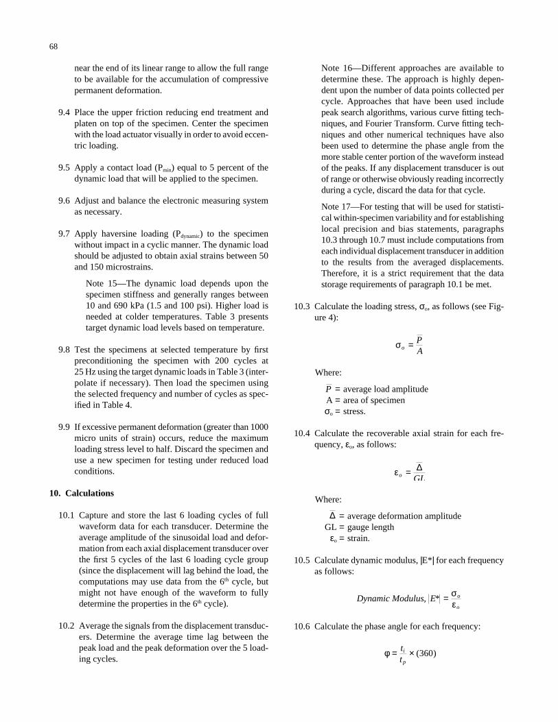
near the end of its linear range to allow the full rangeto be available for the accumulation of compressivepermanent deformation.
9.4 Place the upper friction reducing end treatment andplaten on top of the specimen. Center the specimenwith the load actuator visually in order to avoid eccen-tric loading.
9.5 Apply a contact load (Pmin) equal to 5 percent of thedynamic load that will be applied to the specimen.
9.6 Adjust and balance the electronic measuring systemas necessary.
9.7 Apply haversine loading (Pdynamic) to the specimenwithout impact in a cyclic manner. The dynamic loadshould be adjusted to obtain axial strains between 50and 150 microstrains.
Note 15—The dynamic load depends upon thespecimen stiffness and generally ranges between10 and 690 kPa (1.5 and 100 psi). Higher load isneeded at colder temperatures. Table 3 presentstarget dynamic load levels based on temperature.
9.8 Test the specimens at selected temperature by firstpreconditioning the specimen with 200 cycles at 25 Hz using the target dynamic loads in Table 3 (inter-polate if necessary). Then load the specimen usingthe selected frequency and number of cycles as spec-ified in Table 4.
9.9 If excessive permanent deformation (greater than 1000micro units of strain) occurs, reduce the maximumloading stress level to half. Discard the specimen anduse a new specimen for testing under reduced loadconditions.
10. Calculations
10.1 Capture and store the last 6 loading cycles of fullwaveform data for each transducer. Determine theaverage amplitude of the sinusoidal load and defor-mation from each axial displacement transducer overthe first 5 cycles of the last 6 loading cycle group(since the displacement will lag behind the load, thecomputations may use data from the 6th cycle, butmight not have enough of the waveform to fullydetermine the properties in the 6th cycle).
10.2 Average the signals from the displacement transduc-ers. Determine the average time lag between thepeak load and the peak deformation over the 5 load-ing cycles.
68
Note 16—Different approaches are available todetermine these. The approach is highly depen-dent upon the number of data points collected percycle. Approaches that have been used includepeak search algorithms, various curve fitting tech-niques, and Fourier Transform. Curve fitting tech-niques and other numerical techniques have alsobeen used to determine the phase angle from themore stable center portion of the waveform insteadof the peaks. If any displacement transducer is outof range or otherwise obviously reading incorrectlyduring a cycle, discard the data for that cycle.
Note 17—For testing that will be used for statisti-cal within-specimen variability and for establishinglocal precision and bias statements, paragraphs10.3 through 10.7 must include computations fromeach individual displacement transducer in additionto the results from the averaged displacements.Therefore, it is a strict requirement that the datastorage requirements of paragraph 10.1 be met.
10.3 Calculate the loading stress, σo, as follows (see Fig-ure 4):
Where:
= average load amplitudeA = area of specimenσo = stress.
10.4 Calculate the recoverable axial strain for each fre-quency, εo, as follows:
Where:
= average deformation amplitude GL = gauge length
εo = strain.
10.5 Calculate dynamic modulus, |E*| for each frequencyas follows:
10.6 Calculate the phase angle for each frequency:
φ = ×tt
i
p( )360
Dynamic Modulus E o
o, * = σ
ε
∆
εo GL= ∆
P
σoPA
=
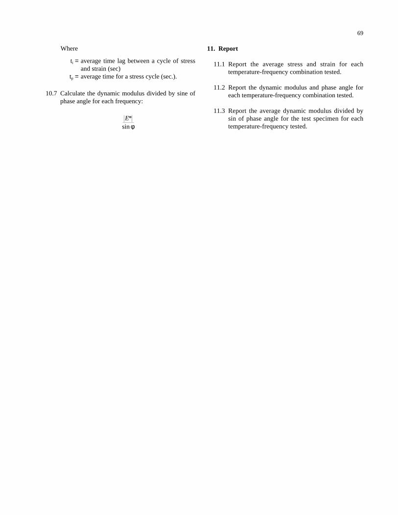
69
Where
ti = average time lag between a cycle of stressand strain (sec)
tp = average time for a stress cycle (sec.).
10.7 Calculate the dynamic modulus divided by sine ofphase angle for each frequency:
E*sin φ
11. Report
11.1 Report the average stress and strain for eachtemperature-frequency combination tested.
11.2 Report the dynamic modulus and phase angle foreach temperature-frequency combination tested.
11.3 Report the average dynamic modulus divided bysin of phase angle for the test specimen for eachtemperature-frequency tested.
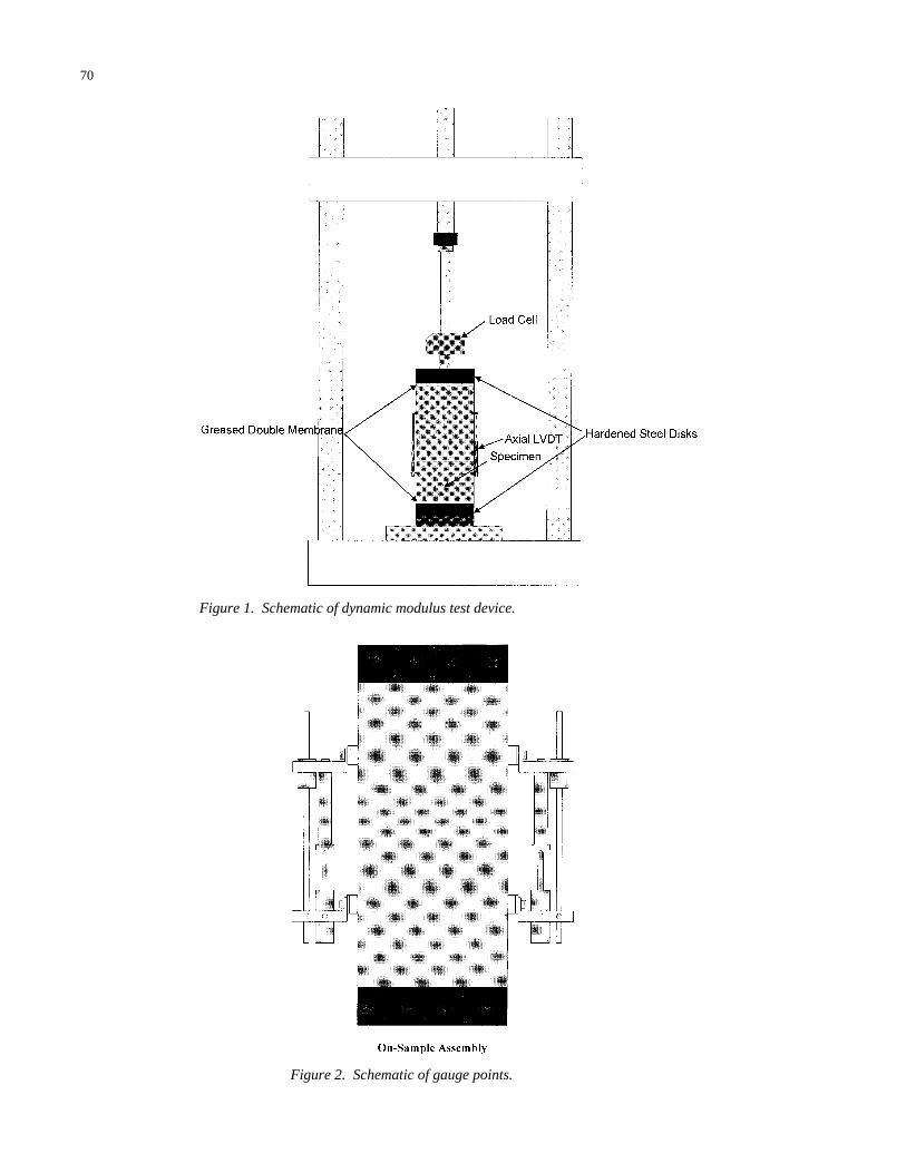
Figure 1. Schematic of dynamic modulus test device.
Figure 2. Schematic of gauge points.
70
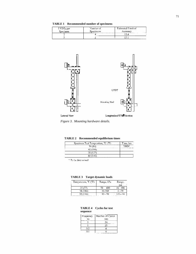
71
TABLE 1 Recommended number of specimens
Figure 3. Mounting hardware details.
TABLE 2 Recommended equilibrium times
TABLE 3 Target dynamic loads
TABLE 4 Cycles for testsequence
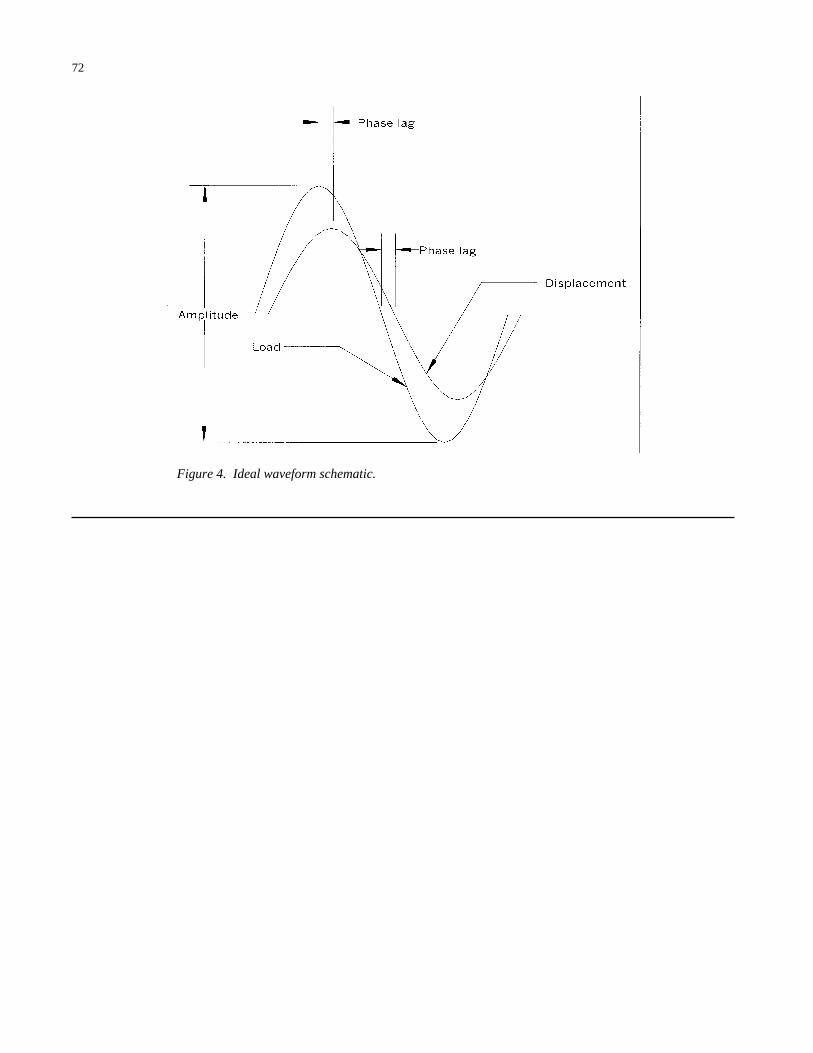
72
Figure 4. Ideal waveform schematic.
73
APPENDIX B
TEST METHOD FOR REPEATED LOAD TESTING OF ASPHALT CONCRETEMIXTURES IN UNIAXIAL COMPRESSION
1. Scope
1.1 This test method covers procedures for the preparation,testing and measurement of permanent deformation ofcylindrical asphalt concrete specimens in a triaxial stateof compressive loading.
1.2 The procedure uses a loading cycle of 1.0 second induration, and consisting of applying 0.1-second haver-sine load followed by 0.9-second rest period. Perma-nent axial and/or radial strains are recorded throughout the test.
1.3 The test is conducted at a single effective temperatureTeff and design stress levels.
1.4 This standard is applicable to laboratory preparedspecimens 100 mm in diameter and 150 mm in heightfor mixtures with nominal maximum size aggregateless than or equal to 37.5 mm (1.5 in).
1.5 This standard may involve hazardous material, oper-ations, and equipment. This standard does not pur-port to address all safety problems associated with itsuse. It is the responsibility of the user of this proce-dure to establish appropriate safety and health prac-tices and to determine the applicability of regulatorylimitations prior to use.
2. Referenced Documents
2.1 AASHTO Standards
TP4 Method for Preparing and Determining theDensity of Hot Mix Asphalt (HMA) Spec-imens by Means of the SHRP GyratoryCompactor
PP2 Practice for Mixture Conditioning of HotMix Asphalt (HMA)
T67 Standard Practices for Load Verificationof Testing Machines (cross-listed withASTM E4)
T269 Percent Air Voids in Compacted Denseand Open Bituminous Paving Mixtures
3. Definitions
3.1 Permanent Deformation—is a manifestation of twodifferent mechanisms and is a combination of densifi-
cation (volume change) and repetitive shear deforma-tion (plastic flow with no volume change).
3.2 Flow Number—is defined as the number of load rep-etitions at which shear deformation, under constantvolume, starts.
3.3 Effective Temperature Teff—Is a single test tempera-ture at which an amount of permanent deformationwould occur equivalent to that measured by consider-ing each season separately throughout the year.
4. Summary of Method
4.1 A cylindrical sample of bituminous paving mixture issubjected to a haversine axial load. The load is appliedfor duration of 0.1-second with a rest period of 0.9-second. The rest period has a load equivalent tothe seating load. The test can be performed eitherwithout confinement, or a confining pressure isapplied to better simulate in situ stress conditions.Cumulative permanent axial and radial strains arerecorded throughout the test. In addition, the numberof repetitions at which shear deformation, under con-stant volume, starts is defined as the Flow Number.
5. Significance and Use
5.1 Current Superpave volumetric mix design procedurelacks a fundamental design criterion to evaluate fun-damental engineering properties of the asphalt mix-ture that directly affect performance. In this test, theselection of the design binder content and aggregatestructure is fundamentally enhanced by the evaluationof the mix resistance to shear flow (Flow Number ofRepetitions).
5.2 This fundamental engineering property can be used asa performance criteria indicator for permanent defor-mation resistance of the asphalt concrete mixture, orcan be simply used to compare the shear resistanceproperties of various bituminous paving mixtures.
6. Apparatus
6.1 Load Test System—A load test system consisting ofa testing machine, environmental chamber, measuringsystem, and specimen end fixtures.
6.1.1 Testing Machine—The testing machine should becapable of applying haversine loads up to 25 kN(5,600 1bs). An electro-hydraulic machine is rec-ommended but not necessarily required. Theloading device should be calibrated as outlined inthe “Equipment Calibration” Section of the test-ing manual.
6.1.2 Confining Pressure Device—A system capable ofmaintaining a constant confining pressure, up to207 kPa (30 psi), such as an air pressure intensi-fier or a hydraulic pump. The device shall beequipped with a pressure relief valve and a sys-tem to pressurize and depressurize the cell withgas or fluid. The device should also have a hightemperature control subsystem for testing up to60°C (140°F) within an accuracy of ±0.5°C (1°F)at constant pressure.
Note 1—It has been found that feedback control ofa servovalve to control the pressure is the preferredmethod of control. However, manual valves or pro-portional valves may be adequate for some applica-tions. The axisymmetric triaxial cells of AASHTOT292 or T294 may be used for this purpose. Othertypes of triaxial cells may be permitted. In all cases,see-through cells are not recommended for use withgas confining media. Sight glass ports or reducedarea windows are recommended with gas media forsafety reasons. It is not required that the specimenbe visible through the cell wall if specimen center-ing and proper instrumentation operation can beverified without a see-through pressure vessel. Cer-tain simulations of pavement loads and extendedmaterial characterization desired for local con-ditions may suggest using confining pressuresgreater than 207 kPa. For pressures higher than690 kPa (100 psi), fluid cells are recommended.
6.1.3 Environmental Chamber—A chamber forcontrolling the test specimen at the desiredtemperature is required. The environmentalchamber shall be capable of controlling thetemperature of the specimen over a tempera-ture range from 25 to 60°C (77 to 140°F ) toan accuracy of ±0.5°C (1°F). The chambershall be large enough to accommodate the testspecimen and a dummy specimen with tem-perature sensor mounted at the center for tem-perature verification.
Note 2—If the chamber does not have sufficientroom for a dummy specimen, it is permissible tohave a second chamber controlling the temperatureof the dummy. The separate dummy chamber mustbe operated similar to the operation of the main test
74
specimen chamber so that the dummy will accu-rately register the time required to obtain tempera-ture equilibrium on the test specimen.
6.1.4 Measurement System—The system shall includea data acquisition system comprising analog todigital conversion and/or digital input for storageand analysis on a computer. The system shall becapable of measuring and recording the time his-tory of the applied load, axial and radial defor-mations for the time duration required by this testmethod. The system shall be capable of measur-ing the load and resulting deformations with aresolution of 0.5 percent.
6.1.4.1 Load—The load shall be measured with anelectronic load cell having adequate capacityfor the anticipated load requirements. Theload cell shall be calibrated in accordancewith AASHTO T67. The load measuringtransducer shall have accuracy equal to orbetter than 0.25 percent of full scale.
Note 3—A 25 kN (5600 lbf) load cell has beenfound to be the approximate maximum capacitylimit for this test method because of range versusresolution factors. It is recommended that if theselected load cell capacity is 25 kN or greater, thesystem should be equipped with either manual orautomatic amplification selection capability so thatit can be used to enhance control of the system atlower anticipated loads.
6.1.4.2 Axial and Radial Deformations—Axial and/orradial deformations shall be measured withdisplacement transducers referenced to gaugepoints contacting the specimen as shown inFigure 1. The axial deformations shall bemeasured at a minimum of two locations180o apart (in plan view); radial deforma-tions shall be measured at a minimum of fourlocations aligned, in planform, on diametral,perpendicular lines which intersect at the cen-ter of the specimen.
Note 4—Analog transducers such as linear vari-able differential transformers (LVDTs) having arange of ±0.5 mm (0.02 in) and inherent nonlin-earity equal to or better than ±0.025 percent of fullscale have been found adequate for this purpose.Software or firmware linearization techniques maybe used to improve the inherent nonlinearity.Amplification and signal conditioning techniquesmay be used with the ±0.5 mm range LVDTs toobtain resolutions down to 0.001mm (0.00004 in)or better for small strain test conditions. These
techniques may be manual or automatic. In gen-eral, increasing the resolution by manual signalamplification will result in reduction of the overallrange of the instrument by the same factor.
6.1.5 Loading Platens—Platens, with a diameter equalto or greater than that of the test specimen arerequired above and below the specimen to trans-fer the load from the testing machine to the spec-imen. Generally, these platens should be made ofhardened or plated steel, or anodized high strengthaluminum. Softer materials will require more fre-quent replacement. Materials that have linearelastic modulus properties and hardness proper-ties lower than that of 6061-T6 aluminum shallnot be used.
6.1.6 Flexible Membrane—For the confined tests, thespecimen should be enclosed in an impermeableflexible membrane. The membrane should be suf-ficiently long to extend well onto the platens andwhen slightly stretched be of the same diameteras the specimen. Typical membrane wall thick-ness ranges between 0.012 and 0.0625 inches(0.305–1.588 mm).
6.1.7 End Treatment—Friction reducing end treatmentsshall be placed between the specimen ends andthe loading platens.
Note 5—End treatments consisting of two 0.5 mm(0.02 in) thick latex sheets separated with siliconegrease have been found to be suitable frictionreducing end treatments.
6.2 Gyratory Compactor—A gyratory compactor andassociated equipment for preparing laboratory speci-mens in accordance with AASHTO TP4 shall be used.Field cores shall meet the requirements of paragraphs7.4 through 7.6 of this test method and any reports oncores so tested will contain a detailed description ofthe location of any lift boundaries within the height ofthe specimen (e.g. lift order, thickness and materialhomogeneity).
6.3 Saw—A machine for sawing test specimen ends to theappropriate length is required. The saw machine shallbe capable of cutting specimens to the prescribeddimensions without excessive heating or shock.
Note 6—A diamond masonry saw greatly facili-tates the preparation of test specimens with smooth,parallel ends. Both single- or double-bladed dia-mond saws should have feed mechanisms and speedcontrols of sufficient precision to ensure compli-ance with paragraphs 7.5 and 7.6 of this method.
75
Adequate blade stiffness is also important to con-trol flexing of the blade during thin cuts.
6.4 Core Drill—A coring machine with cooling systemand a diamond bit for cutting nominal 100 mm (4 in)diameter test specimens.
Note 7—A coring machine with adjustable verticalfeed and rotational speed is recommended. Thevariable feeds and speeds may be controlled by var-ious methods. A vertical feed rate of approximately0.05 mm/rev (0.002 in/rev) and a rotational speedof approximately 455 RPM has been found to besatisfactory for several of the Superpave mixtures.
7. Test Specimens
7.1 Size—Testing shall be performed on 100 mm (4 in)diameter by 150 mm (6 in) high test specimens coredfrom gyratory compacted mixtures.
7.2 Aging—Mixtures shall be aged in accordance with theshort-term oven aging procedure in AASHTO PP2.
7.3 Gyratory Specimens—Prepare 165 mm (6.5 in) highspecimens to the required air void content in accor-dance with AASHTO TP-4.
7.4 Coring—Core the nominal 100 mm (4 in) diametertest specimens from the center of the gyratory speci-mens. Both the core drill and the gyratory specimenshould be adequately supported to ensure that theresulting test specimen is cylindrical with sides thatare smooth, parallel, and free from steps, ridges, andgrooves.
7.5 Diameter—Measure the diameter of the test specimenat the mid-height and third points along axes that are90 degrees apart. Record each of the six measure-ments to the nearest 1 mm (0.05 in). Calculate theaverage and the standard deviation of the six mea-surements. If the standard deviation is greater than 2.5 mm (0.01 in) discard the specimen. For acceptablespecimens, the average diameter, reported to the near-est 1 mm, shall be used in the stress calculations.
7.6 End Preparation—The ends of all test specimens shallbe smooth and perpendicular to the axis of the speci-men. Prepare the ends of the specimen by sawing witha single- or double-bladed saw. To ensure that thesawed samples have parallel ends, the prepared speci-men ends shall meet the tolerances described below.Reject test specimens not meeting these tolerances.
7.6.1 The specimen ends shall have a cut surface wavi-ness height within a tolerance of ±0.05 mm across
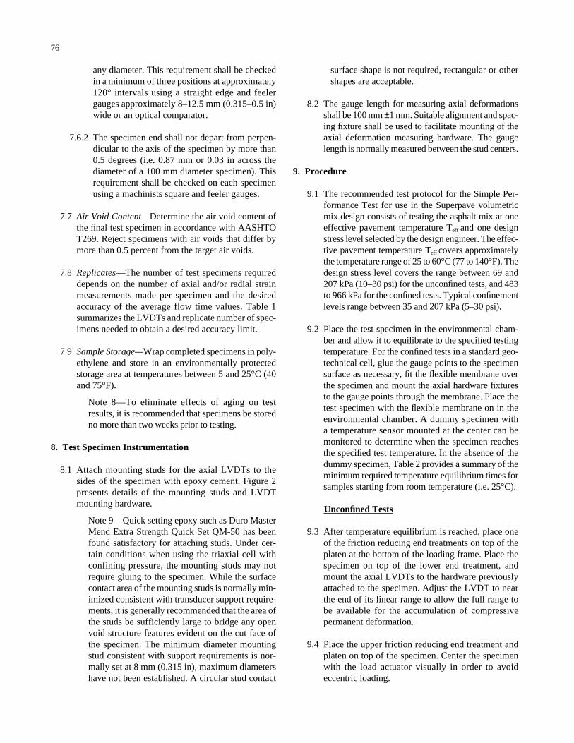
any diameter. This requirement shall be checkedin a minimum of three positions at approximately120° intervals using a straight edge and feelergauges approximately 8–12.5 mm (0.315–0.5 in)wide or an optical comparator.
7.6.2 The specimen end shall not depart from perpen-dicular to the axis of the specimen by more than0.5 degrees (i.e. 0.87 mm or 0.03 in across thediameter of a 100 mm diameter specimen). Thisrequirement shall be checked on each specimenusing a machinists square and feeler gauges.
7.7 Air Void Content—Determine the air void content ofthe final test specimen in accordance with AASHTOT269. Reject specimens with air voids that differ bymore than 0.5 percent from the target air voids.
7.8 Replicates—The number of test specimens requireddepends on the number of axial and/or radial strainmeasurements made per specimen and the desiredaccuracy of the average flow time values. Table 1summarizes the LVDTs and replicate number of spec-imens needed to obtain a desired accuracy limit.
7.9 Sample Storage—Wrap completed specimens in poly-ethylene and store in an environmentally protectedstorage area at temperatures between 5 and 25°C (40and 75°F).
Note 8—To eliminate effects of aging on testresults, it is recommended that specimens be storedno more than two weeks prior to testing.
8. Test Specimen Instrumentation
8.1 Attach mounting studs for the axial LVDTs to thesides of the specimen with epoxy cement. Figure 2presents details of the mounting studs and LVDTmounting hardware.
Note 9—Quick setting epoxy such as Duro MasterMend Extra Strength Quick Set QM-50 has beenfound satisfactory for attaching studs. Under cer-tain conditions when using the triaxial cell withconfining pressure, the mounting studs may notrequire gluing to the specimen. While the surfacecontact area of the mounting studs is normally min-imized consistent with transducer support require-ments, it is generally recommended that the area ofthe studs be sufficiently large to bridge any openvoid structure features evident on the cut face ofthe specimen. The minimum diameter mountingstud consistent with support requirements is nor-mally set at 8 mm (0.315 in), maximum diametershave not been established. A circular stud contact
76
surface shape is not required, rectangular or othershapes are acceptable.
8.2 The gauge length for measuring axial deformationsshall be 100 mm ±1 mm. Suitable alignment and spac-ing fixture shall be used to facilitate mounting of theaxial deformation measuring hardware. The gaugelength is normally measured between the stud centers.
9. Procedure
9.1 The recommended test protocol for the Simple Per-formance Test for use in the Superpave volumetricmix design consists of testing the asphalt mix at oneeffective pavement temperature Teff and one designstress level selected by the design engineer. The effec-tive pavement temperature Teff covers approximatelythe temperature range of 25 to 60°C (77 to 140°F). Thedesign stress level covers the range between 69 and207 kPa (10–30 psi) for the unconfined tests, and 483to 966 kPa for the confined tests. Typical confinementlevels range between 35 and 207 kPa (5–30 psi).
9.2 Place the test specimen in the environmental cham-ber and allow it to equilibrate to the specified testingtemperature. For the confined tests in a standard geo-technical cell, glue the gauge points to the specimensurface as necessary, fit the flexible membrane overthe specimen and mount the axial hardware fixturesto the gauge points through the membrane. Place thetest specimen with the flexible membrane on in theenvironmental chamber. A dummy specimen witha temperature sensor mounted at the center can bemonitored to determine when the specimen reachesthe specified test temperature. In the absence of thedummy specimen, Table 2 provides a summary of theminimum required temperature equilibrium times forsamples starting from room temperature (i.e. 25°C).
Unconfined Tests
9.3 After temperature equilibrium is reached, place oneof the friction reducing end treatments on top of theplaten at the bottom of the loading frame. Place thespecimen on top of the lower end treatment, andmount the axial LVDTs to the hardware previouslyattached to the specimen. Adjust the LVDT to nearthe end of its linear range to allow the full range tobe available for the accumulation of compressivepermanent deformation.
9.4 Place the upper friction reducing end treatment andplaten on top of the specimen. Center the specimenwith the load actuator visually in order to avoideccentric loading.

9.5 Apply a contact load equal to 5 percent of the totalload that will be applied to the specimen, whileensuring the proper response of the LVDTs (i.e.,check for proper direction sensing for all LVDTs).
9.6 Place the radial LVDTs in contact with the speci-men, adjust the LVDTs to near the end of their lin-ear range to allow the full range to be available forthe accumulation of radial permanent deformation.Adjust and balance the electronic measuring systemas necessary.
9.7 Close the environmental chamber and allow suffi-cient time (normally 10 to 15 minutes) for the tem-perature to stabilize within the specimen and thechamber.
9.8 After the time required for the sample to reach thetesting temperature, apply the haversine load, whichyields the desired stress on the specimen. The maxi-mum applied load (Pmax) is the maximum total loadapplied to the sample, including the contact andcyclic load: Pmax = Pcontact + Pcyclic.
9.9 The contact load (Pcontact) is the vertical load placedon the specimen to maintain a positive contactbetween loading strip and the specimen: Pcontact =0.05 × Pmax.
9.10 The cyclic load (Pcyclic) is the load applied to the testspecimen which is used to calculate the permanentdeformation parameters: Pcyclic = Pmax − Pcontact.
9.11 Apply the haversine loading (Pcyclic) and continueuntil 10,000 cycles (2.8 hours) or until the specimenfails and results in excessive tertiary deformation tothe specimen, whichever comes first. The total num-ber of cycles or the testing time will depend on thetemperature and the stress levels applied.
9.12 During the load applications, record the load applied,the axial and radial deflection measured from allLVDTs through the data acquisition system. Signal-to-noise ratio should be at least 10. All data should becollected in real time and collected/processed so as tominimize phase errors due to sequential channel sam-pling. In order to save storage space during data acqui-sition for 10,000 cycles, it is recommended to use thedata acquisition of the cycles shown in Table 3.
Confined Tests
9.13 After temperature equilibrium is reached, place oneof the friction reducing end treatments on top of theplaten at the bottom of the loading frame. Place the
77
specimen on top of the lower end treatment, placethe top platen and extend the flexible membrane overthe top and bottom platens. Attach the O-rings to sealthe specimen on top and bottom platens from theconfining air/fluid. Center the specimen with theload actuator visually in order to avoid eccentricloading.
9.14 Mount the axial LVDTs to the hardware previouslyattached to the specimen. Adjust the LVDT to nearthe end of its linear range to allow the full range tobe available for the accumulation of compressivepermanent deformation.
9.15 Connect the appropriate hose through the upper orlower platen (or take other appropriate steps) tokeep the specimen’s internal void structure underatmospheric pressure while pressure greater thanatmospheric is applied to the outside of the mem-brane during testing.
9.16 Assemble the triaxial cell over the specimen, ensureproper seal with the base and connect the fluid (orgas) pressure lines.
9.17 Apply a contact load equal to 5 percent of the load thatwill be applied to the specimen, while ensuring theproper response of the LVDTs (i.e., both decreaseaccordingly). Place the radial LVDTs in contactwith the specimen, adjust the LVDTs to near theend of their linear range to allow the full range tobe available for the accumulation of radial perma-nent deformation.
9.18 Record the initial LVDT readings and slowlyincrease the lateral pressure to the desired test level(e.g. 2 psi /sec). Adjust and balance the electronicmeasuring system as necessary. Close the environ-mental chamber and allow sufficient time (normally10 to 15 minutes) for the temperature to stabilizewithin the specimen and the chamber.
9.19 After the time required for the sample to reach thetesting temperature, apply the haversine load, whichyields the desired stress on the specimen. Continueuntil 10,000 cycles (2.8 hours) or until the specimenfails and results in excessive tertiary deformation tothe specimen, whichever comes first. The total num-ber of cycles or the testing time will depend on thetemperature and the stress levels applied.
9.20 During the load applications, record the load applied,confining pressure, the axial and radial deflectionmeasured from all LVDTs through the data acqui-sition system. Signal-to-noise ratio should be at
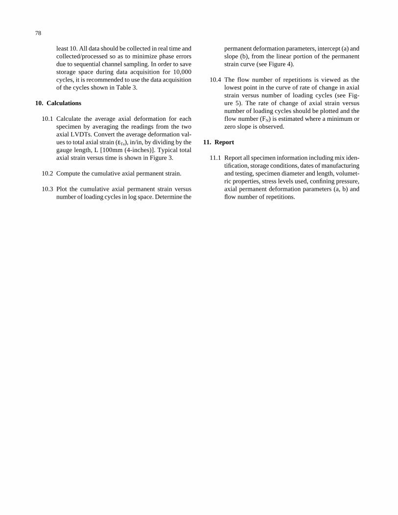
least 10. All data should be collected in real time andcollected/processed so as to minimize phase errorsdue to sequential channel sampling. In order to savestorage space during data acquisition for 10,000cycles, it is recommended to use the data acquisitionof the cycles shown in Table 3.
10. Calculations
10.1 Calculate the average axial deformation for eachspecimen by averaging the readings from the twoaxial LVDTs. Convert the average deformation val-ues to total axial strain (εTa), in/in, by dividing by thegauge length, L [100mm (4-inches)]. Typical totalaxial strain versus time is shown in Figure 3.
10.2 Compute the cumulative axial permanent strain.
10.3 Plot the cumulative axial permanent strain versusnumber of loading cycles in log space. Determine the
78
permanent deformation parameters, intercept (a) andslope (b), from the linear portion of the permanentstrain curve (see Figure 4).
10.4 The flow number of repetitions is viewed as thelowest point in the curve of rate of change in axialstrain versus number of loading cycles (see Fig-ure 5). The rate of change of axial strain versusnumber of loading cycles should be plotted and theflow number (FN) is estimated where a minimum orzero slope is observed.
11. Report
11.1 Report all specimen information including mix iden-tification, storage conditions, dates of manufacturingand testing, specimen diameter and length, volumet-ric properties, stress levels used, confining pressure,axial permanent deformation parameters (a, b) andflow number of repetitions.
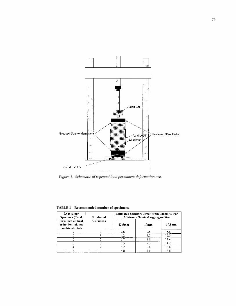
79
Figure 1. Schematic of repeated load permanent deformation test.
TABLE 1 Recommended number of specimens
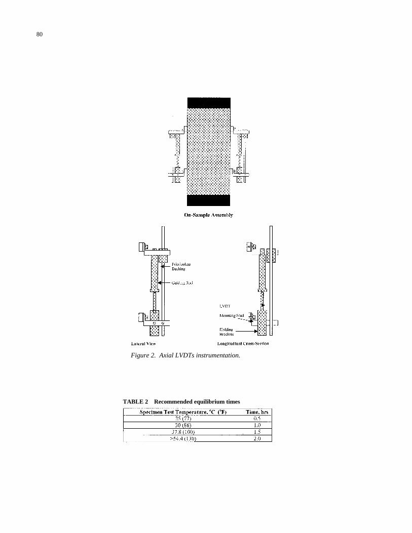
Figure 2. Axial LVDTs instrumentation.
TABLE 2 Recommended equilibrium times
80
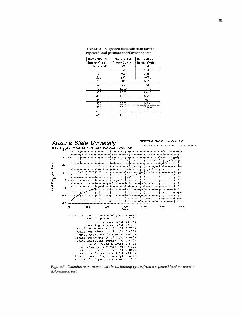
81
TABLE 3 Suggested data collection for therepeated load permanent deformation test
Figure 3. Cumulative permanent strain vs. loading cycles from a repeated load permanentdeformation test.
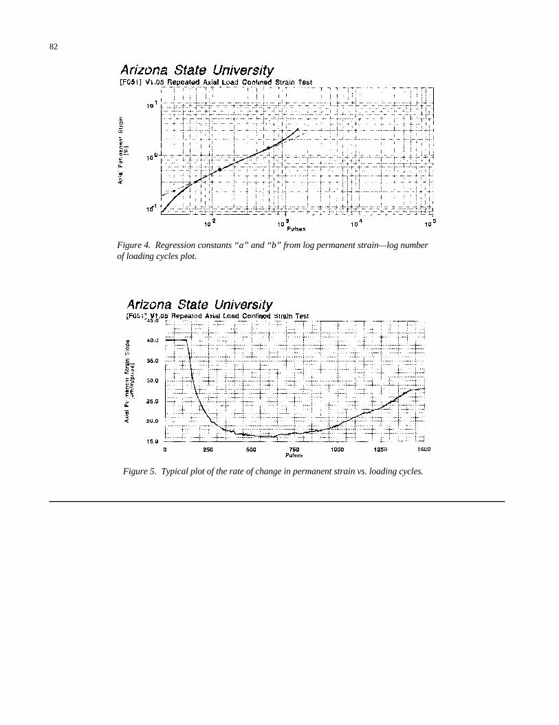
82
Figure 5. Typical plot of the rate of change in permanent strain vs. loading cycles.
Figure 4. Regression constants “a” and “b” from log permanent strain—log numberof loading cycles plot.
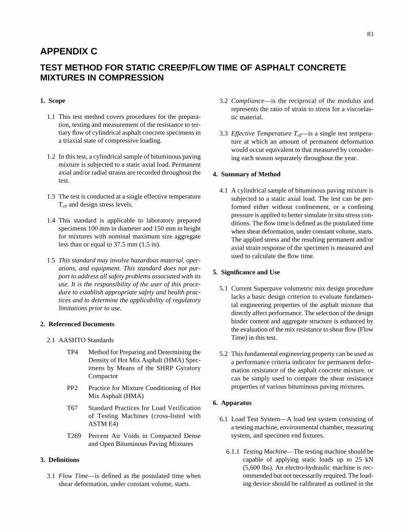
83
APPENDIX C
TEST METHOD FOR STATIC CREEP/FLOW TIME OF ASPHALT CONCRETEMIXTURES IN COMPRESSION
1. Scope
1.1 This test method covers procedures for the prepara-tion, testing and measurement of the resistance to ter-tiary flow of cylindrical asphalt concrete specimens ina triaxial state of compressive loading.
1.2 In this test, a cylindrical sample of bituminous pavingmixture is subjected to a static axial load. Permanentaxial and/or radial strains are recorded throughout thetest.
1.3 The test is conducted at a single effective temperatureTeff and design stress levels.
1.4 This standard is applicable to laboratory preparedspecimens 100 mm in diameter and 150 mm in heightfor mixtures with nominal maximum size aggregateless than or equal to 37.5 mm (1.5 in).
1.5 This standard may involve hazardous material, oper-ations, and equipment. This standard does not pur-port to address all safety problems associated with itsuse. It is the responsibility of the user of this proce-dure to establish appropriate safety and health prac-tices and to determine the applicability of regulatorylimitations prior to use.
2. Referenced Documents
2.1 AASHTO Standards
TP4 Method for Preparing and Determining theDensity of Hot Mix Asphalt (HMA) Spec-imens by Means of the SHRP GyratoryCompactor
PP2 Practice for Mixture Conditioning of HotMix Asphalt (HMA)
T67 Standard Practices for Load Verificationof Testing Machines (cross-listed withASTM E4)
T269 Percent Air Voids in Compacted Denseand Open Bituminous Paving Mixtures
3. Definitions
3.1 Flow Time—is defined as the postulated time whenshear deformation, under constant volume, starts.
3.2 Compliance—is the reciprocal of the modulus andrepresents the ratio of strain to stress for a viscoelas-tic material.
3.3 Effective Temperature Teff—is a single test tempera-ture at which an amount of permanent deformationwould occur equivalent to that measured by consider-ing each season separately throughout the year.
4. Summary of Method
4.1 A cylindrical sample of bituminous paving mixture issubjected to a static axial load. The test can be per-formed either without confinement, or a confiningpressure is applied to better simulate in situ stress con-ditions. The flow time is defined as the postulated timewhen shear deformation, under constant volume, starts.The applied stress and the resulting permanent and/oraxial strain response of the specimen is measured andused to calculate the flow time.
5. Significance and Use
5.1 Current Superpave volumetric mix design procedurelacks a basic design criterion to evaluate fundamen-tal engineering properties of the asphalt mixture thatdirectly affect performance. The selection of the designbinder content and aggregate structure is enhanced bythe evaluation of the mix resistance to shear flow (FlowTime) in this test.
5.2 This fundamental engineering property can be used asa performance criteria indicator for permanent defor-mation resistance of the asphalt concrete mixture, orcan be simply used to compare the shear resistanceproperties of various bituminous paving mixtures.
6. Apparatus
6.1 Load Test System—A load test system consisting ofa testing machine, environmental chamber, measuringsystem, and specimen end fixtures.
6.1.1 Testing Machine—The testing machine should becapable of applying static loads up to 25 kN(5,600 lbs). An electro-hydraulic machine is rec-ommended but not necessarily required. The load-ing device should be calibrated as outlined in the

“Equipment Calibration” Section of the testingmanual.
6.1.2 Confining Pressure Device—A system capable ofmaintaining a constant confining pressure, up to207 kPa (30 psi), such as an air pressure intensi-fier or a hydraulic pump. The device shall beequipped with a pressure relief valve, and a sys-tem to pressurize and depressurize the cell withgas or fluid. The device should also have a hightemperature control subsystem for testing up to60°C (140°F) within an accuracy of ±0.5°C (1°F)at constant pressure.
Note 1—It has been found that feedback control ofa servovalve to control the pressure is the preferredmethod of control. However, manual valves or pro-portional valves may be adequate for some applica-tions. The axisymmetric triaxial cells of AASHTOT292 or T294 may be used for this purpose. Othertypes of triaxial cells may be permitted. In allcases, see-through cells are not recommended foruse with gas confining media. Sight glass ports orreduced area windows are recommended with gasmedia for safety reasons. It is not required that thespecimen be visible through the cell wall if speci-men centering and proper instrumentation opera-tion can be verified without a see-through pressurevessel. Certain simulations of pavement loads andextended material characterization desired for localconditions may suggest using confining pressuresgreater than 207 kPa. For pressures higher than690 kPa (100 psi), fluid cells are recommended.
6.1.3 Environmental Chamber—A chamber for control-ling the test specimen at the desired temperature isrequired. The environmental chamber shall becapable of controlling the temperature of the spec-imen over a temperature range from 25 to 60°C (77to 140°F ) to an accuracy of ±0.5°C (1°F). Thechamber shall be large enough to accommodatethe test specimen and a dummy specimen withtemperature sensor mounted at the center for tem-perature verification.
Note 2—If the chamber does not have sufficientroom for a dummy specimen, it is permissible tohave a second chamber controlling the temperatureof the dummy. The separate dummy chamber mustbe operated similar to the operation of the main testspecimen chamber so that the dummy will accu-rately register the time required to obtain tempera-ture equilibrium on the test specimen.
6.1.4 Measurement System—The system shall includea data acquisition system comprising analog to
84
digital conversion and/or digital input for storageand analysis on a computer. The system shall becapable of measuring and recording the time his-tory of the applied load, axial and radial defor-mations for the time duration required by this testmethod. The system shall be capable of measur-ing the load and resulting deformations with aresolution of 0.5 percent.
6.1.4.1 Load—The load shall be measured with anelectronic load cell having adequate capacityfor the anticipated load requirements. Theload cell shall be calibrated in accordancewith AASHTO T67. The load measuringtransducer shall have accuracy equal to orbetter than 0.25 percent of full scale.
Note 3—A 25 kN (5600 lbf) load cell has beenfound to be the approximate maximum capacitylimit for this test method because of range versusresolution factors. It is recommended that if theselected load cell capacity is 25 kN or greater, thesystem should be equipped with either manual orautomatic amplification selection capability so thatit can be used to enhance control of the system atlower anticipated loads.
6.1.4.2 Axial and Radial Deformations—Axialand/or radial deformations shall be measuredwith displacement transducers referenced togauge points contacting the specimen asshown in Figure 1. The axial deformationsshall be measured at a minimum of two loca-tions 180° apart (in plan view); radial defor-mations shall be measured at a minimum offour locations aligned, in planform, on diame-tral, perpendicular lines which intersect at thecenter of the specimen.
Note 4—Analog transducers such as linear vari-able differential transformers (LVDTs) having arange of ±0.5 mm (0.02 in) and inherent nonlin-earity equal to or better than ±0.025 percent of fullscale have been found adequate for this purpose.Software or firmware linearization techniques maybe used to improve the inherent nonlinearity.Amplification and signal conditioning techniquesmay be used with the ±0.5 mm range LVDTs toobtain resolutions down to 0.001mm (0.00004 in)or better for small strain test conditions. Thesetechniques may be manual or automatic. In gen-eral, increasing the resolution by manual signalamplification will result in reduction of the overallrange of the instrument by the same factor.
6.1.5 Loading Platens—Platens, with a diameter equalto or greater than that of the test specimen are
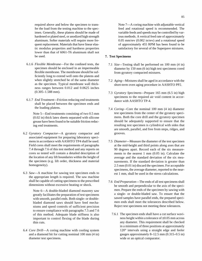
required above and below the specimen to trans-fer the load from the testing machine to the spec-imen. Generally, these platens should be made ofhardened or plated steel, or anodized high strengthaluminum. Softer materials will require more fre-quent replacement. Materials that have linear elas-tic modulus properties and hardness propertieslower than that of 6061-T6 aluminum shall notbe used.
6.1.6 Flexible Membrane—For the confined tests, thespecimen should be enclosed in an impermeableflexible membrane. The membrane should be suf-ficiently long to extend well onto the platens andwhen slightly stretched be of the same diameteras the specimen. Typical membrane wall thick-ness ranges between 0.012 and 0.0625 inches(0.305–1.588 mm).
6.1.7 End Treatment—Friction reducing end treatmentsshall be placed between the specimen ends andthe loading platens.
Note 5—End treatments consisting of two 0.5 mm(0.02 in) thick latex sheets separated with siliconegrease have been found to be suitable friction reduc-ing end treatments.
6.2 Gyratory Compactor—A gyratory compactor andassociated equipment for preparing laboratory speci-mens in accordance with AASHTO TP4 shall be used.Field cores shall meet the requirements of paragraphs7.4 through 7.6 of this test method and any reports oncores so tested will contain a detailed description ofthe location of any lift boundaries within the height ofthe specimen (e.g. lift order, thickness and materialhomogeneity).
6.3 Saw—A machine for sawing test specimen ends to the appropriate length is required. The saw machineshall be capable of cutting specimens to the prescribeddimensions without excessive heating or shock.
Note 6—A double-bladed diamond masonry sawgreatly facilitates the preparation of test specimenswith smooth, parallel ends. Both single- or double-bladed diamond saws should have feed mecha-nisms and speed controls of sufficient precisionto ensure compliance with paragraphs 7.5 and 7.6of this method. Adequate blade stiffness is alsoimportant to control flexing of the blade duringthin cuts.
6.4 Core Drill—A coring machine with cooling systemand a diamond bit for cutting nominal 100 mm (4 in)diameter test specimens.
85
Note 7—A coring machine with adjustable verticalfeed and rotational speed is recommended. Thevariable feeds and speeds may be controlled by var-ious methods. A vertical feed rate of approximately0.05 mm/rev (0.002 in/rev) and a rotational speedof approximately 455 RPM has been found to besatisfactory for several of the Superpave mixtures.
7. Test Specimens
7.1 Size—Testing shall be performed on 100 mm (4 in)diameter by 150 mm (6 in) high test specimens coredfrom gyratory compacted mixtures.
7.2 Aging—Mixtures shall be aged in accordance with theshort-term oven aging procedure in AASHTO PP2.
7.3 Gyratory Specimens—Prepare 165 mm (6.5 in) highspecimens to the required air void content in accor-dance with AASHTO TP-4.
7.4 Coring—Core the nominal 100 mm (4 in) diametertest specimens from the center of the gyratory speci-mens. Both the core drill and the gyratory specimenshould be adequately supported to ensure that theresulting test specimen is cylindrical with sides thatare smooth, parallel, and free from steps, ridges, andgrooves.
7.5 Diameter—Measure the diameter of the test specimenat the mid-height and third points along axes that are90 degrees apart. Record each of the six measure-ments to the nearest 1 mm (0.05 in). Calculate theaverage and the standard deviation of the six mea-surements. If the standard deviation is greater than2.5 mm (0.01 in) discard the specimen. For acceptablespecimens, the average diameter, reported to the near-est 1 mm, shall be used in the stress calculations.
7.6 End Preparation—The ends of all test specimens shallbe smooth and perpendicular to the axis of the speci-men. Prepare the ends of the specimen by sawing witha single- or double-bladed saw. To ensure that thesawed samples have parallel ends, the prepared speci-men ends shall meet the tolerances described below.Reject test specimens not meeting these tolerances.
7.6.1 The specimen ends shall have a cut surface wavi-ness height within a tolerance of ±0.05 mm acrossany diameter. This requirement shall be checkedin a minimum of three positions at approximately120° intervals using a straight edge and feelergauges approximately 8–12.5 mm (0.315–0.5 in)wide or an optical comparator.
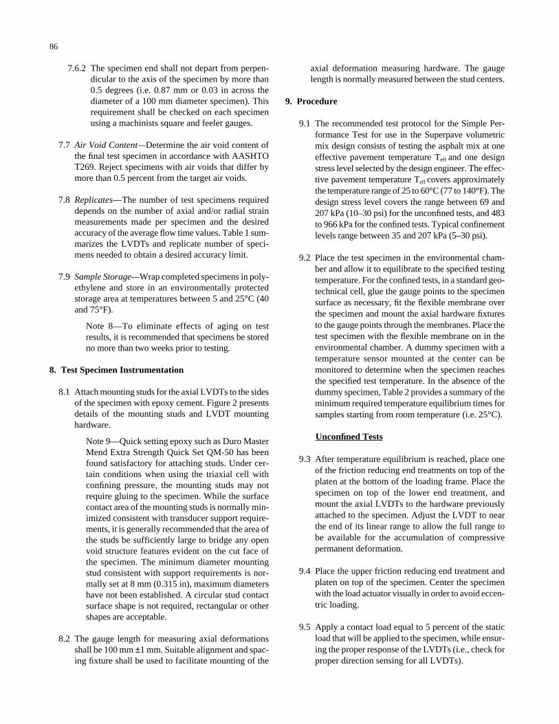
7.6.2 The specimen end shall not depart from perpen-dicular to the axis of the specimen by more than0.5 degrees (i.e. 0.87 mm or 0.03 in across thediameter of a 100 mm diameter specimen). Thisrequirement shall be checked on each specimenusing a machinists square and feeler gauges.
7.7 Air Void Content—Determine the air void content ofthe final test specimen in accordance with AASHTOT269. Reject specimens with air voids that differ bymore than 0.5 percent from the target air voids.
7.8 Replicates—The number of test specimens requireddepends on the number of axial and/or radial strainmeasurements made per specimen and the desiredaccuracy of the average flow time values. Table 1 sum-marizes the LVDTs and replicate number of speci-mens needed to obtain a desired accuracy limit.
7.9 Sample Storage—Wrap completed specimens in poly-ethylene and store in an environmentally protectedstorage area at temperatures between 5 and 25°C (40and 75°F).
Note 8—To eliminate effects of aging on testresults, it is recommended that specimens be storedno more than two weeks prior to testing.
8. Test Specimen Instrumentation
8.1 Attach mounting studs for the axial LVDTs to the sidesof the specimen with epoxy cement. Figure 2 presentsdetails of the mounting studs and LVDT mountinghardware.
Note 9—Quick setting epoxy such as Duro MasterMend Extra Strength Quick Set QM-50 has beenfound satisfactory for attaching studs. Under cer-tain conditions when using the triaxial cell withconfining pressure, the mounting studs may notrequire gluing to the specimen. While the surfacecontact area of the mounting studs is normally min-imized consistent with transducer support require-ments, it is generally recommended that the area ofthe studs be sufficiently large to bridge any openvoid structure features evident on the cut face ofthe specimen. The minimum diameter mountingstud consistent with support requirements is nor-mally set at 8 mm (0.315 in), maximum diametershave not been established. A circular stud contactsurface shape is not required, rectangular or othershapes are acceptable.
8.2 The gauge length for measuring axial deformationsshall be 100 mm ±1 mm. Suitable alignment and spac-ing fixture shall be used to facilitate mounting of the
86
axial deformation measuring hardware. The gaugelength is normally measured between the stud centers.
9. Procedure
9.1 The recommended test protocol for the Simple Per-formance Test for use in the Superpave volumetricmix design consists of testing the asphalt mix at oneeffective pavement temperature Teff and one designstress level selected by the design engineer. The effec-tive pavement temperature Teff covers approximatelythe temperature range of 25 to 60°C (77 to 140°F). Thedesign stress level covers the range between 69 and207 kPa (10–30 psi) for the unconfined tests, and 483to 966 kPa for the confined tests. Typical confinementlevels range between 35 and 207 kPa (5–30 psi).
9.2 Place the test specimen in the environmental cham-ber and allow it to equilibrate to the specified testingtemperature. For the confined tests, in a standard geo-technical cell, glue the gauge points to the specimensurface as necessary, fit the flexible membrane overthe specimen and mount the axial hardware fixturesto the gauge points through the membranes. Place thetest specimen with the flexible membrane on in theenvironmental chamber. A dummy specimen with atemperature sensor mounted at the center can bemonitored to determine when the specimen reachesthe specified test temperature. In the absence of thedummy specimen, Table 2 provides a summary of theminimum required temperature equilibrium times forsamples starting from room temperature (i.e. 25°C).
Unconfined Tests
9.3 After temperature equilibrium is reached, place oneof the friction reducing end treatments on top of theplaten at the bottom of the loading frame. Place thespecimen on top of the lower end treatment, andmount the axial LVDTs to the hardware previouslyattached to the specimen. Adjust the LVDT to nearthe end of its linear range to allow the full range tobe available for the accumulation of compressivepermanent deformation.
9.4 Place the upper friction reducing end treatment andplaten on top of the specimen. Center the specimenwith the load actuator visually in order to avoid eccen-tric loading.
9.5 Apply a contact load equal to 5 percent of the staticload that will be applied to the specimen, while ensur-ing the proper response of the LVDTs (i.e., check forproper direction sensing for all LVDTs).
9.6 Place the radial LVDTs in contact with the speci-men, adjust the LVDTs to near the end of their lin-ear range to allow the full range to be available forthe accumulation of radial permanent deformation.Adjust and balance the electronic measuring systemas necessary.
9.7 Close the environmental chamber and allow sufficienttime (normally 10 to 15 minutes) for the temperatureto stabilize within the specimen and the chamber.
9.8 After the time required for the sample to reach thetesting temperature, apply a rapid axial static load atapproximately 15 MPa/sec to obtain the desiredstress on the specimen.
9.9 Hold the load constant until tertiary flow occurs orthe total axial strain reaches approximately 2%. Thetest time will depend on the temperature and thestress levels applied.
9.10 During the load application, record the load applied,the axial and radial deflection measured from allLVDTs through the data acquisition system.
Confined Tests
9.11 After temperature equilibrium is reached, place oneof the friction reducing end treatments on top of theplaten at the bottom of the loading frame. Place thespecimen on top of the lower end treatment, placethe top platen and extend the flexible membrane overthe top and bottom platens. Attach the O-rings to sealthe specimen on top and bottom platens from theconfining air/fluid. Center the specimen with theload actuator visually in order to avoid eccentricloading.
9.12 Mount the axial LVDTs to the hardware previouslyattached to the specimen. Adjust the LVDT to nearthe end of its linear range to allow the full range tobe available for the accumulation of compressivepermanent deformation.
9.13 Connect the appropriate hose through the upper orlower platen (or take other appropriate steps) tokeep the specimen’s internal void structure underatmospheric pressure while pressure greater thanatmospheric is applied to the outside of the mem-brane during testing.
9.14 Assemble the triaxial cell over the specimen, ensureproper seal with the base and connect the fluid (orgas) pressure lines.
87
9.15 Apply a contact load equal to 5 percent of the staticload that will be applied to the specimen, whileensuring the proper response of the LVDTs (i.e.,both decrease accordingly). Place the radial LVDTsin contact with the specimen, adjust the LVDTs tonear the end of their linear range to allow the fullrange to be available for the accumulation of radialpermanent deformation.
9.16 Record the initial LVDT readings and slowlyincrease the lateral pressure to the desired test level(e.g. 2 psi /sec). Adjust and balance the electronicmeasuring system as necessary. Close the environ-mental chamber and allow sufficient time (normally10 to 15 minutes) for the temperature to stabilizewithin the specimen and the chamber
9.17 After the time required for the sample to reach thetesting temperature, apply a rapid axial static load atapproximately 15 MPa/sec to obtain the desired devi-atoric stress on the specimen. Hold the load constantuntil the tertiary flow occurs or the total axial strainreaches 4–5%. The test time will depend on the tem-perature and the stress levels applied.
9.18 During the load application, record the load, confin-ing pressure, the axial and radial deflection measuredfrom all LVDTs through the data acquisition system.
10. Calculations
10.1 Calculate the average axial deformation for eachspecimen by averaging the readings from the twoaxial LVDTs. Convert the average deformation val-ues to total axial strain (εTa), in/in, by dividing by thegauge length, L [100mm (4-inches)]. Typical totalaxial strain versus time is shown in Figure 3.
10.2 Compute the total axial compliance D(t) = εT /σd ,where σd is the deviator stress applied during testingin psi. (σd = applied constant load [lb] divided by thecross sectional area of the specimen [in2]).
10.3 Plot the total axial compliance versus time in logspace.
10.4 Using the data generated between the total axialcompliance and time, determine the axial creep com-pliance parameters (Do, D1, M1) from the linear por-tion of the creep compliance data between a time often seconds until the end of the linear curve (see Fig-ure 4). The creep compliance parameters are esti-mated as follows:
Do: is the instantaneous compliance, and can beassumed to be the value of the total compliance at
a time equal to 100 ms (if the load is appliedrapidly at 50 ms).
D1: is the intercept of the creep compliance–time rela-tionship, which is the estimated value of the totalcompliance at a time of one second.
M1: is the slope of the creep compliance–time rela-tionship.
10.5 The flow point is viewed as the lowest point in thecurve of rate of change in axial compliance versusloading time (see Figure 5). The rate of change ofcreep compliance D′(t) versus loading time shouldbe plotted and the flow time (Ft) is estimated usingthe following mathematical procedure:
Ten data points are taken from every log scale unitof time at approximately equal intervals. Then, at aspecific time t1, a polynomial equation is fitted usingfive points (two points forward and two points back-ward from the time t1). The form of this equation is:
D(t)I = a + bt + ct2
Where
D(t)1 = compliance at time t for t1 point evaluatedt = time of loading
a,b,c = regression coefficients
88
By taking the derivative of the above equation, oneobtains the following:
Therefore, the rate of change in compliance at timeti is equal to b + 2cti. For each data point selected onecan obtain the rate of change in compliance byrepeating the above procedure. Once all the rates ofchange in compliance are calculated, one can find thezero value of rate of change in compliance, i.e., theflow point. This is accomplished by another poly-nomial curve fit, using equal data points on bothsides of the minimum value. Theoretically the “flowpoint” is the time corresponding to a rate of compli-ance change equal to zero.
11. Report
11.1 Report all specimen information including mix iden-tification, storage conditions, dates of manufacturingand testing, specimen diameter and length, volumet-ric properties, stress levels used, confining pressure,creep compliance parameters (Do, D1, M1) and flowtime.
d(D(t) )dt
b 2cti = +
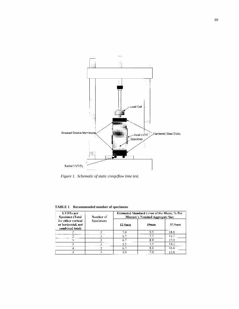
89
Figure 1. Schematic of static creep/flow time test.
TABLE 1 Recommended number of specimens
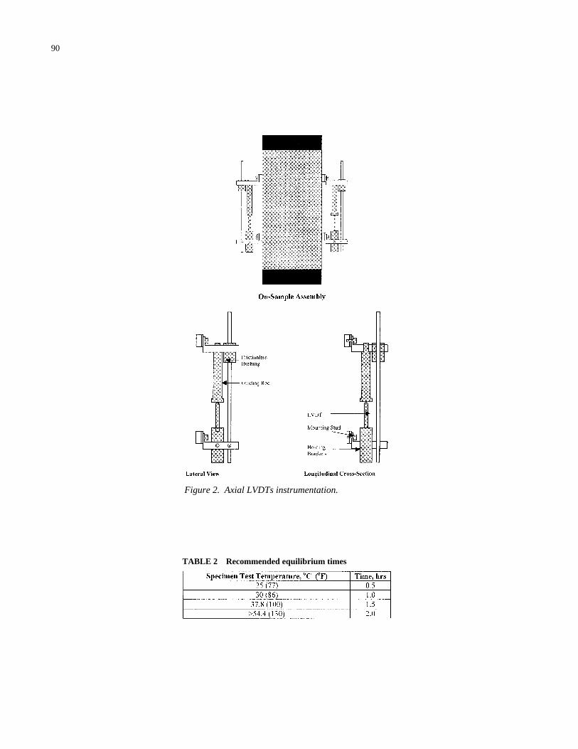
90
Figure 2. Axial LVDTs instrumentation.
TABLE 2 Recommended equilibrium times
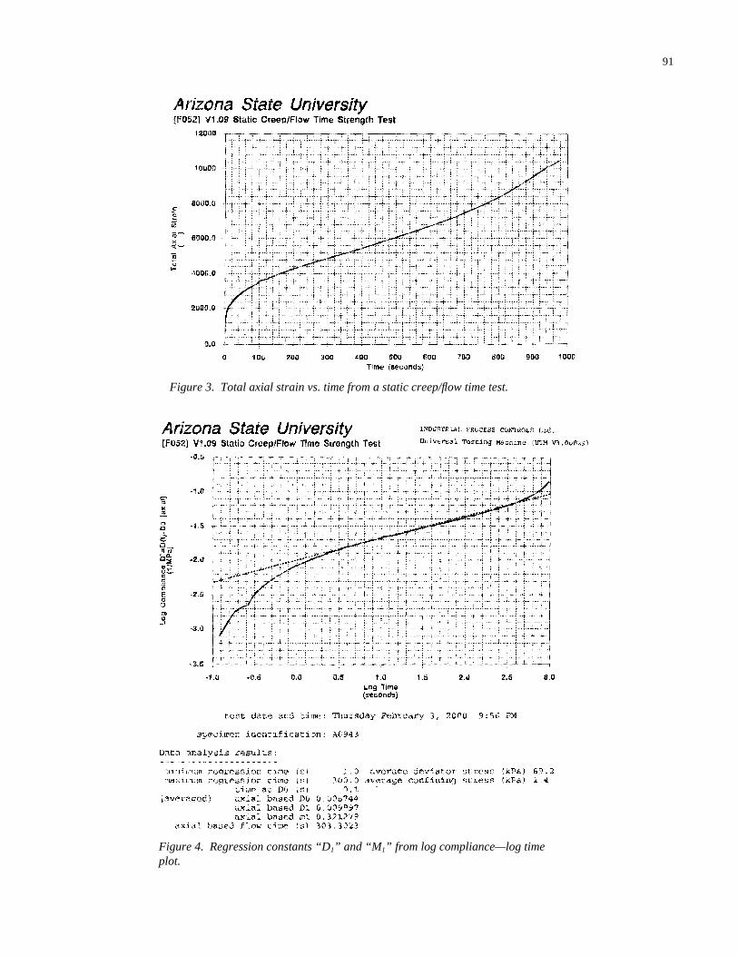
91
Figure 3. Total axial strain vs. time from a static creep/flow time test.
Figure 4. Regression constants “D1” and “M1” from log compliance—log timeplot.
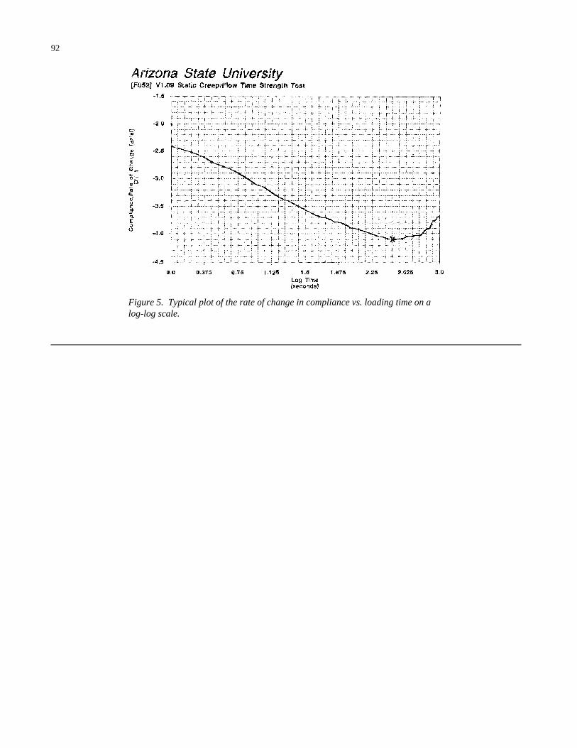
92
Figure 5. Typical plot of the rate of change in compliance vs. loading time on alog-log scale.
93
APPENDIX D
TEST METHOD FOR DYNAMIC MODULUS OF ASPHALT CONCRETE MIXTURESFOR FATIGUE CRACKING
1. Scope
1.1 This test method covers procedures for preparing andtesting asphalt concrete mixtures to determine thedynamic modulus and phase angle at a single effectivetemperature Teff and design loading frequency.
1.2 This test method is a part of test protocols thatinclude determination of the dynamic modulus of theasphalt mix for paving purposes. The other testmethods are Standard Test Method for Simple Per-formance Test for Permanent Deformation BasedUpon Dynamic Modulus of Asphalt Concrete Mix-ture and Standard Test Method for Dynamic Modulusof Asphalt Concrete Mixtures, which is for construct-ing a master curve for characterizing asphalt concretefor pavement thickness design and performanceanalysis.
1.3 This standard is applicable to laboratory prepared spec-imens of mixtures with nominal maximum size aggre-gate less than or equal to 37.5 mm (1.5 in).
1.4 This standard may involve hazardous material, oper-ations, and equipment. This standard does not pur-port to address all safety problems associated with itsuse. It is the responsibility of the user of this proce-dure to establish appropriate safety and health prac-tices and to determine the applicability of regulatorylimitations prior to use.
2. Referenced Documents
2.1 AASHTO Standards
TP4 Method for Preparing and Determining theDensity of Hot Mix Asphalt (HMA) Spec-imens by Means of the SHRP GyratoryCompactor
PP2 Practice for Mixture Conditioning of HotMix Asphalt (HMA)
T67 Standard Practices for Load Verificationof Testing Machines (cross-listed withASTM E4)
T269 Percent Air Voids in Compacted Dense andOpen Bituminous Paving Mixtures
3. Definitions
3.1 Dynamic Modulus—|E*|, the norm value of the com-plex modulus calculated by dividing the peak-to-peakstress by the peak-to-peak strain for a material sub-jected to a sinusoidal loading.
3.2 Complex Modulus—E*, a complex number that definesthe relationship between stress and strain for a linearviscoelastic material.
3.3 Phase angle—δ, the angle in degrees between a sinu-soidally applied stress and the resulting strain in acontrolled-stress test.
3.4 Linear viscoelastic—within the context of this test,refers to behavior in which the dynamic modulus isindependent of stress or strain amplitude.
3.5 Effective Temperature Teff—Is a single test tempera-ture at which an amount of fatigue cracking wouldoccur equivalent to that measured by considering eachseason separately throughout the year.
4. Summary of Method
4.1 A sinusoidal (haversine) axial compressive stress isapplied to a specimen of asphalt concrete at a giventemperature and loading frequency. The applied stressand the resulting recoverable axial strain response ofthe specimen is measured and used to calculate thedynamic modulus and phase angle.
4.2 Figure 1 presents a schematic of the dynamic modu-lus test device.
5. Significance and Use
5.1 Dynamic modulus values, measured at one effectivetemperature Teff and one design frequency selected bythe design engineer, are used as performance criteriafor fatigue cracking resistance of the asphalt concretemixture to be used in conjunction with the SuperpaveVolumetric Mix Design Method.
Note 1—The effective temperature Teff coversapproximately the temperature range of 4 to 20°C(39 to 68°F).
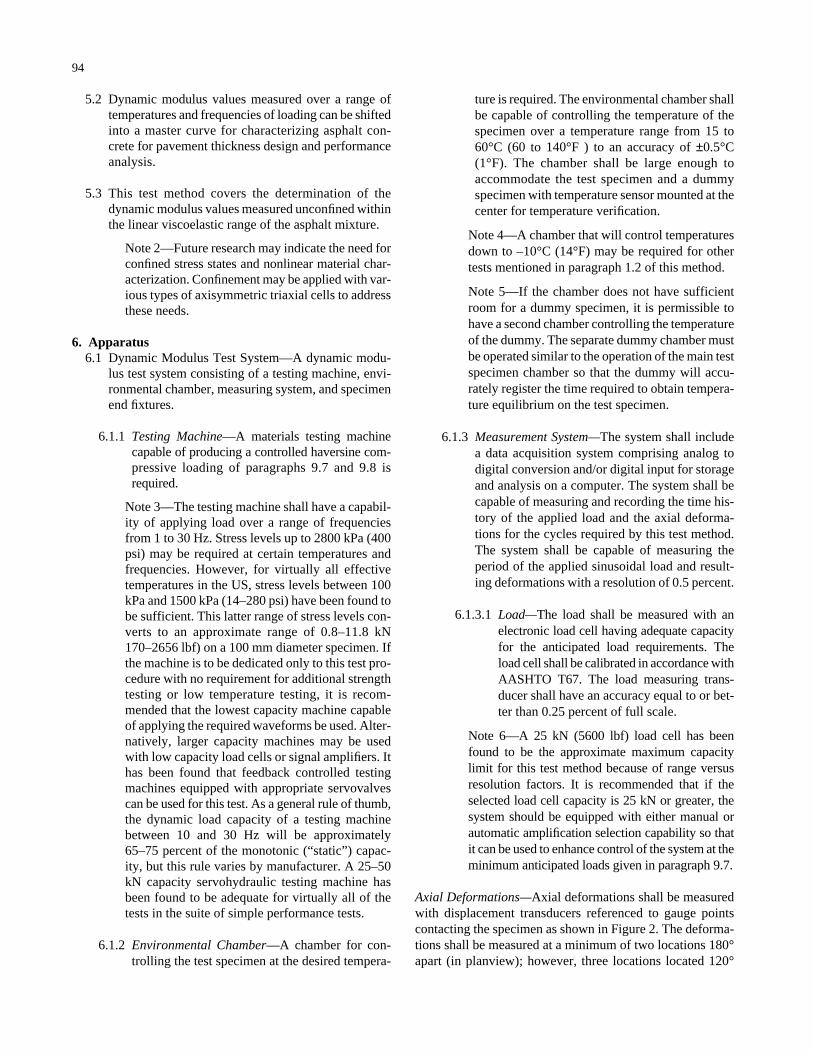
5.2 Dynamic modulus values measured over a range oftemperatures and frequencies of loading can be shiftedinto a master curve for characterizing asphalt con-crete for pavement thickness design and performanceanalysis.
5.3 This test method covers the determination of thedynamic modulus values measured unconfined withinthe linear viscoelastic range of the asphalt mixture.
Note 2—Future research may indicate the need forconfined stress states and nonlinear material char-acterization. Confinement may be applied with var-ious types of axisymmetric triaxial cells to addressthese needs.
6. Apparatus6.1 Dynamic Modulus Test System—A dynamic modu-
lus test system consisting of a testing machine, envi-ronmental chamber, measuring system, and specimenend fixtures.
6.1.1 Testing Machine—A materials testing machinecapable of producing a controlled haversine com-pressive loading of paragraphs 9.7 and 9.8 isrequired.
Note 3—The testing machine shall have a capabil-ity of applying load over a range of frequenciesfrom 1 to 30 Hz. Stress levels up to 2800 kPa (400psi) may be required at certain temperatures andfrequencies. However, for virtually all effectivetemperatures in the US, stress levels between 100kPa and 1500 kPa (14–280 psi) have been found tobe sufficient. This latter range of stress levels con-verts to an approximate range of 0.8–11.8 kN170–2656 lbf) on a 100 mm diameter specimen. Ifthe machine is to be dedicated only to this test pro-cedure with no requirement for additional strengthtesting or low temperature testing, it is recom-mended that the lowest capacity machine capableof applying the required waveforms be used. Alter-natively, larger capacity machines may be usedwith low capacity load cells or signal amplifiers. Ithas been found that feedback controlled testingmachines equipped with appropriate servovalvescan be used for this test. As a general rule of thumb,the dynamic load capacity of a testing machinebetween 10 and 30 Hz will be approximately65–75 percent of the monotonic (“static”) capac-ity, but this rule varies by manufacturer. A 25–50kN capacity servohydraulic testing machine hasbeen found to be adequate for virtually all of thetests in the suite of simple performance tests.
6.1.2 Environmental Chamber—A chamber for con-trolling the test specimen at the desired tempera-
94
ture is required. The environmental chamber shallbe capable of controlling the temperature of thespecimen over a temperature range from 15 to60°C (60 to 140°F ) to an accuracy of ±0.5°C(1°F). The chamber shall be large enough toaccommodate the test specimen and a dummyspecimen with temperature sensor mounted at thecenter for temperature verification.
Note 4—A chamber that will control temperaturesdown to –10°C (14°F) may be required for othertests mentioned in paragraph 1.2 of this method.
Note 5—If the chamber does not have sufficientroom for a dummy specimen, it is permissible tohave a second chamber controlling the temperatureof the dummy. The separate dummy chamber mustbe operated similar to the operation of the main testspecimen chamber so that the dummy will accu-rately register the time required to obtain tempera-ture equilibrium on the test specimen.
6.1.3 Measurement System—The system shall includea data acquisition system comprising analog todigital conversion and/or digital input for storageand analysis on a computer. The system shall becapable of measuring and recording the time his-tory of the applied load and the axial deforma-tions for the cycles required by this test method.The system shall be capable of measuring theperiod of the applied sinusoidal load and result-ing deformations with a resolution of 0.5 percent.
6.1.3.1 Load—The load shall be measured with anelectronic load cell having adequate capacityfor the anticipated load requirements. Theload cell shall be calibrated in accordance withAASHTO T67. The load measuring trans-ducer shall have an accuracy equal to or bet-ter than 0.25 percent of full scale.
Note 6—A 25 kN (5600 lbf) load cell has beenfound to be the approximate maximum capacitylimit for this test method because of range versusresolution factors. It is recommended that if theselected load cell capacity is 25 kN or greater, thesystem should be equipped with either manual orautomatic amplification selection capability so thatit can be used to enhance control of the system at theminimum anticipated loads given in paragraph 9.7.
Axial Deformations—Axial deformations shall be measuredwith displacement transducers referenced to gauge pointscontacting the specimen as shown in Figure 2. The deforma-tions shall be measured at a minimum of two locations 180°apart (in planview); however, three locations located 120°
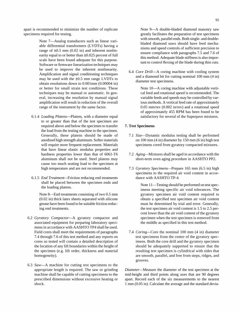
apart is recommended to minimize the number of replicatespecimens required for testing.
Note 7—Analog transducers such as linear vari-able differential transformers (LVDTs) having arange of ±0.5 mm (0.02 in) and inherent nonlin-earity equal to or better than ±0.025 percent of fullscale have been found adequate for this purpose.Software or firmware linearization techniques maybe used to improve the inherent nonlinearity.Amplification and signal conditioning techniquesmay be used with the ±0.5 mm range LVDTs toobtain resolutions down to 0.001mm (0.00004 in)or better for small strain test conditions. Thesetechniques may be manual or automatic. In gen-eral, increasing the resolution by manual signalamplification will result in reduction of the overallrange of the instrument by the same factor.
6.1.4 Loading Platens—Platens, with a diameter equalto or greater than that of the test specimen arerequired above and below the specimen to transferthe load from the testing machine to the specimen.Generally, these platens should be made ofanodized high strength aluminum. Softer materialswill require more frequent replacement. Materialsthat have linear elastic modulus properties andhardness properties lower than that of 6061-T6aluminum shall not be used. Steel platens maycause too much seating load to the specimen athigh temperature and are not recommended.
6.1.5 End Treatment—Friction reducing end treatmentsshall be placed between the specimen ends andthe loading platens.
Note 8—End treatments consisting of two 0.5 mm(0.02 in) thick latex sheets separated with siliconegrease have been found to be suitable friction reduc-ing end treatments.
6.2 Gyratory Compactor—A gyratory compactor andassociated equipment for preparing laboratory speci-mens in accordance with AASHTO TP4 shall be used.Field cores shall meet the requirements of paragraphs7.4 through 7.6 of this test method and any reports oncores so tested will contain a detailed description ofthe location of any lift boundaries within the height ofthe specimen (e.g. lift order, thickness and materialhomogeneity).
6.3 Saw—A machine for cutting test specimens to theappropriate length is required. The saw or grindingmachine shall be capable of cutting specimens to theprescribed dimensions without excessive heating orshock.
95
Note 9—A double-bladed diamond masonry sawgreatly facilitates the preparation of test specimenswith smooth, parallel ends. Both single- and double-bladed diamond saws should have feed mecha-nisms and speed controls of sufficient precision toensure compliance with paragraphs 7.5 and 7.6 ofthis method. Adequate blade stiffness is also impor-tant to control flexing of the blade during thin cuts.
6.4 Core Drill—A coring machine with cooling systemand a diamond bit for cutting nominal 100 mm (4 in)diameter test specimens.
Note 10—A coring machine with adjustable verti-cal feed and rotational speed is recommended. Thevariable feeds and speeds may be controlled by var-ious methods. A vertical feed rate of approximately0.05 mm/rev (0.002 in/rev) and a rotational speedof approximately 455 RPM has been found to besatisfactory for several of the Superpave mixtures.
7. Test Specimens
7.1 Size—Dynamic modulus testing shall be performedon 100 mm (4 in) diameter by 150 mm (6 in) high testspecimens cored from gyratory compacted mixtures.
7.2 Aging—Mixtures shall be aged in accordance with theshort-term oven aging procedure in AASHTO PP2.
7.3 Gyratory Specimens—Prepare 165 mm (6.5 in) highspecimens to the required air void content in accor-dance with AASHTO TP-4.
Note 11—Testing should be performed on test spec-imens meeting specific air void tolerances. Thegyratory specimen air void content required toobtain a specified test specimen air void contentmust be determined by trial and error. Generally,the test specimen air void content is 1.5 to 2.5 per-cent lower than the air void content of the gyratoryspecimen when the test specimen is removed fromthe middle as specified in this test method.
7.4 Coring—Core the nominal 100 mm (4 in) diametertest specimens from the center of the gyratory spec-imens. Both the core drill and the gyratory specimenshould be adequately supported to ensure that theresulting test specimen is cylindrical with sides thatare smooth, parallel, and free from steps, ridges, andgrooves.
Diameter—Measure the diameter of the test specimen at themid-height and third points along axes that are 90 degreesapart. Record each of the six measurements to the nearest 1 mm (0.05 in). Calculate the average and the standard devia-
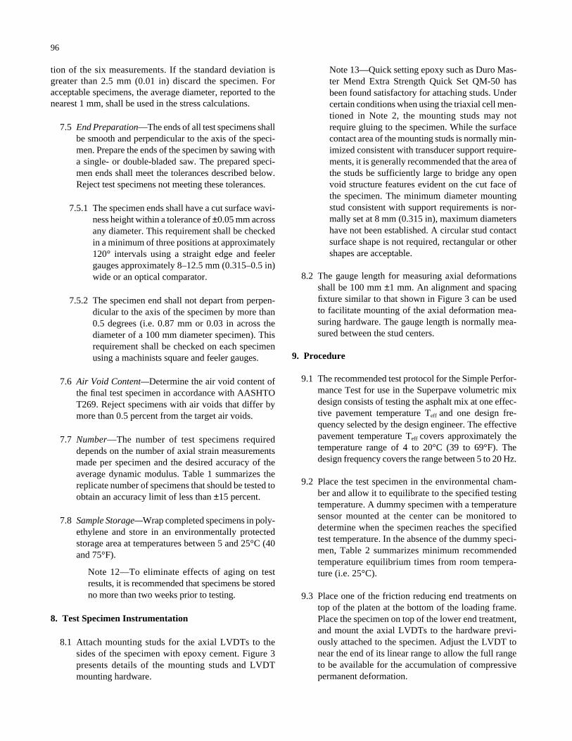
tion of the six measurements. If the standard deviation isgreater than 2.5 mm (0.01 in) discard the specimen. Foracceptable specimens, the average diameter, reported to thenearest 1 mm, shall be used in the stress calculations.
7.5 End Preparation—The ends of all test specimens shallbe smooth and perpendicular to the axis of the speci-men. Prepare the ends of the specimen by sawing witha single- or double-bladed saw. The prepared speci-men ends shall meet the tolerances described below.Reject test specimens not meeting these tolerances.
7.5.1 The specimen ends shall have a cut surface wavi-ness height within a tolerance of ±0.05 mm acrossany diameter. This requirement shall be checkedin a minimum of three positions at approximately120° intervals using a straight edge and feelergauges approximately 8–12.5 mm (0.315–0.5 in)wide or an optical comparator.
7.5.2 The specimen end shall not depart from perpen-dicular to the axis of the specimen by more than0.5 degrees (i.e. 0.87 mm or 0.03 in across thediameter of a 100 mm diameter specimen). Thisrequirement shall be checked on each specimenusing a machinists square and feeler gauges.
7.6 Air Void Content—Determine the air void content ofthe final test specimen in accordance with AASHTOT269. Reject specimens with air voids that differ bymore than 0.5 percent from the target air voids.
7.7 Number—The number of test specimens requireddepends on the number of axial strain measurementsmade per specimen and the desired accuracy of theaverage dynamic modulus. Table 1 summarizes thereplicate number of specimens that should be tested toobtain an accuracy limit of less than ±15 percent.
7.8 Sample Storage—Wrap completed specimens in poly-ethylene and store in an environmentally protectedstorage area at temperatures between 5 and 25°C (40and 75°F).
Note 12—To eliminate effects of aging on testresults, it is recommended that specimens be storedno more than two weeks prior to testing.
8. Test Specimen Instrumentation
8.1 Attach mounting studs for the axial LVDTs to thesides of the specimen with epoxy cement. Figure 3presents details of the mounting studs and LVDTmounting hardware.
96
Note 13—Quick setting epoxy such as Duro Mas-ter Mend Extra Strength Quick Set QM-50 hasbeen found satisfactory for attaching studs. Undercertain conditions when using the triaxial cell men-tioned in Note 2, the mounting studs may notrequire gluing to the specimen. While the surfacecontact area of the mounting studs is normally min-imized consistent with transducer support require-ments, it is generally recommended that the area ofthe studs be sufficiently large to bridge any openvoid structure features evident on the cut face ofthe specimen. The minimum diameter mountingstud consistent with support requirements is nor-mally set at 8 mm (0.315 in), maximum diametershave not been established. A circular stud contactsurface shape is not required, rectangular or othershapes are acceptable.
8.2 The gauge length for measuring axial deformationsshall be 100 mm ±1 mm. An alignment and spacingfixture similar to that shown in Figure 3 can be usedto facilitate mounting of the axial deformation mea-suring hardware. The gauge length is normally mea-sured between the stud centers.
9. Procedure
9.1 The recommended test protocol for the Simple Perfor-mance Test for use in the Superpave volumetric mixdesign consists of testing the asphalt mix at one effec-tive pavement temperature Teff and one design fre-quency selected by the design engineer. The effectivepavement temperature Teff covers approximately thetemperature range of 4 to 20°C (39 to 69°F). Thedesign frequency covers the range between 5 to 20 Hz.
9.2 Place the test specimen in the environmental cham-ber and allow it to equilibrate to the specified testingtemperature. A dummy specimen with a temperaturesensor mounted at the center can be monitored todetermine when the specimen reaches the specifiedtest temperature. In the absence of the dummy speci-men, Table 2 summarizes minimum recommendedtemperature equilibrium times from room tempera-ture (i.e. 25°C).
9.3 Place one of the friction reducing end treatments ontop of the platen at the bottom of the loading frame.Place the specimen on top of the lower end treatment,and mount the axial LVDTs to the hardware previ-ously attached to the specimen. Adjust the LVDT tonear the end of its linear range to allow the full rangeto be available for the accumulation of compressivepermanent deformation.
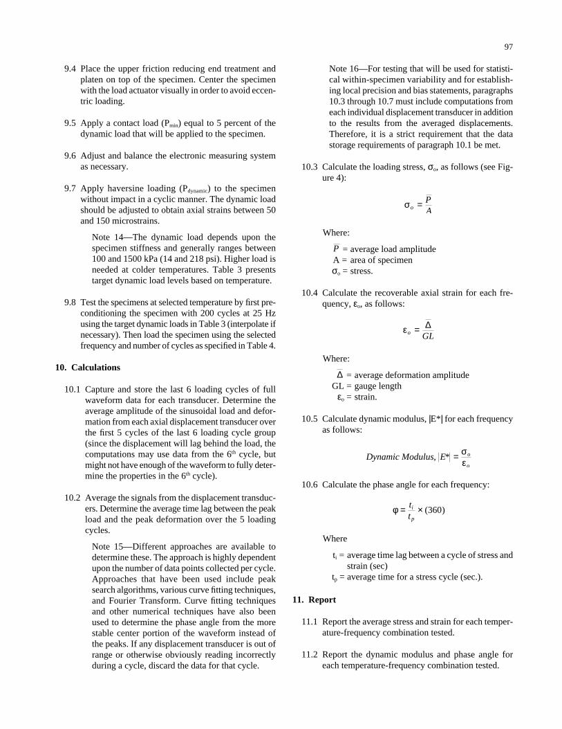
9.4 Place the upper friction reducing end treatment andplaten on top of the specimen. Center the specimenwith the load actuator visually in order to avoid eccen-tric loading.
9.5 Apply a contact load (Pmin) equal to 5 percent of thedynamic load that will be applied to the specimen.
9.6 Adjust and balance the electronic measuring systemas necessary.
9.7 Apply haversine loading (Pdynamic) to the specimenwithout impact in a cyclic manner. The dynamic loadshould be adjusted to obtain axial strains between 50and 150 microstrains.
Note 14—The dynamic load depends upon thespecimen stiffness and generally ranges between100 and 1500 kPa (14 and 218 psi). Higher load isneeded at colder temperatures. Table 3 presentstarget dynamic load levels based on temperature.
9.8 Test the specimens at selected temperature by first pre-conditioning the specimen with 200 cycles at 25 Hzusing the target dynamic loads in Table 3 (interpolate ifnecessary). Then load the specimen using the selectedfrequency and number of cycles as specified in Table 4.
10. Calculations
10.1 Capture and store the last 6 loading cycles of fullwaveform data for each transducer. Determine theaverage amplitude of the sinusoidal load and defor-mation from each axial displacement transducer overthe first 5 cycles of the last 6 loading cycle group(since the displacement will lag behind the load, thecomputations may use data from the 6th cycle, butmight not have enough of the waveform to fully deter-mine the properties in the 6th cycle).
10.2 Average the signals from the displacement transduc-ers. Determine the average time lag between the peakload and the peak deformation over the 5 loadingcycles.
Note 15—Different approaches are available todetermine these. The approach is highly dependentupon the number of data points collected per cycle.Approaches that have been used include peaksearch algorithms, various curve fitting techniques,and Fourier Transform. Curve fitting techniquesand other numerical techniques have also beenused to determine the phase angle from the morestable center portion of the waveform instead ofthe peaks. If any displacement transducer is out ofrange or otherwise obviously reading incorrectlyduring a cycle, discard the data for that cycle.
97
Note 16—For testing that will be used for statisti-cal within-specimen variability and for establish-ing local precision and bias statements, paragraphs10.3 through 10.7 must include computations fromeach individual displacement transducer in additionto the results from the averaged displacements.Therefore, it is a strict requirement that the datastorage requirements of paragraph 10.1 be met.
10.3 Calculate the loading stress, σo, as follows (see Fig-ure 4):
Where:
= average load amplitudeA = area of specimenσo = stress.
10.4 Calculate the recoverable axial strain for each fre-quency, εo, as follows:
Where:
= average deformation amplitudeGL = gauge length
εo = strain.
10.5 Calculate dynamic modulus, |E*| for each frequencyas follows:
10.6 Calculate the phase angle for each frequency:
Where
ti = average time lag between a cycle of stress andstrain (sec)
tp = average time for a stress cycle (sec.).
11. Report
11.1 Report the average stress and strain for each temper-ature-frequency combination tested.
11.2 Report the dynamic modulus and phase angle foreach temperature-frequency combination tested.
φ = ×tt
i
p( )360
Dynamic Modulus E o
o, * = σ
ε
∆
εo GL= ∆
P
σoPA
=
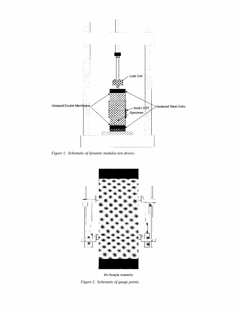
Figure 1. Schematic of dynamic modulus test device.
Figure 2. Schematic of gauge points.
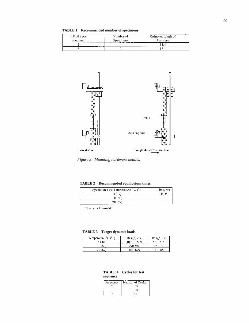
99
TABLE 1 Recommended number of specimens
Figure 3. Mounting hardware details.
TABLE 2 Recommended equilibrium times
TABLE 3 Target dynamic loads
TABLE 4 Cycles for testsequence
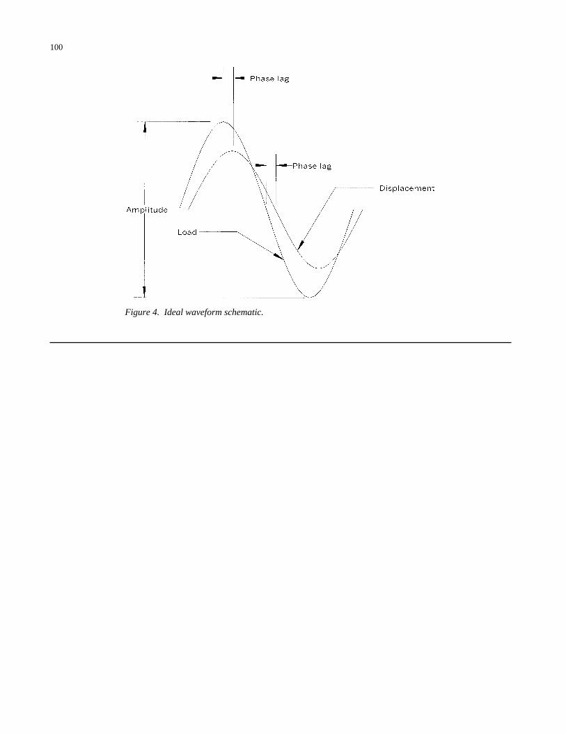
100
Figure 4. Ideal waveform schematic.

101
APPENDIX E
TEST METHOD FOR INDIRECT TENSILE CREEP TESTING OF ASPHALTMIXTURES FOR THERMAL CRACKING
1. Scope
1.1 This test method covers procedures for preparing andtesting asphalt concrete mixtures to determine the creepcompliance at a given temperature and stress level.
1.2 In this test, a disc sample of bituminous paving mix-ture is subjected to a diametral static creep load. Hori-zontal and vertical deformations are recorded through-out the test (vertical deformations are required only ifPoisson’s ratio is to be calculated from the test results).
1.3 This standard is applicable to laboratory prepared spec-imens of mixtures with nominal maximum size aggre-gate less than or equal to 19.0 mm (0.75 in).
1.4 This standard may involve hazardous material, oper-ations, and equipment. This standard does not pur-port to address all safety problems associated with itsuse. It is the responsibility of the user of this proce-dure to establish appropriate safety and health prac-tices and to determine the applicability of regulatorylimitations prior to use.
2. Referenced Documents
2.1 AASHTO Standards
TP4 Method for Preparing and Determiningthe Density of Hot Mix Asphalt (HMA)Specimens by Means of the SHRP Gyra-tory Compactor
PP2 Practice for Mixture Conditioning of HotMix Asphalt (HMA)
T269 Percent Air Voids in Compacted Denseand Open Bituminous Paving Mixtures
TP9-94 Standard Test Method for Determining theCreep Compliance and Strength of HotMix Asphalt (HMA) Using the IndirectTensile Test Device
3. Definitions
3.1 Creep—The time-dependent part of strain resultingfrom stress.
3.2 Tensile Strength—St, the strength shown by a speci-men subjected to tension.
3.3 Creep Compliance—D(t), the time-dependent straindivided by the applied stress.
4. Summary of Method
4.1 This standard describes two procedures, the tensilestrength and the tensile creep. Both testings are deter-mined for thermal cracking analyses.
4.2 Tensile strength is determined by applying a constantrate of vertical deformation (ram movement) to failure.
4.3 The tensile creep is determined by applying a staticload of fixed magnitude (percentage of the tensilestrength) along the diametral axis of a specimen. Thehorizontal and vertical deformations measured nearthe center of the specimen are used to calculate tensilecreep compliance as a function of time (vertical defor-mations are required only if Poisson’s ratio is to becalculated from the test results). By measuring defor-mations in regions with relatively constant stressesand away from the localized non-linear effects inducedby the steel loading strips, Poisson’s ratio can be moreaccurately determined.
5. Significance and Use
5.1 Tensile strength and tensile creep test data are requiredto determine the master relaxation modulus curveand fracture parameters used for the thermal fractureanalysis.
5.2 The values of creep compliance and tensile strengthcan be used in linear visco-elastic analysis to calculatethe fatigue cracking potential of asphalt concrete.
6. Apparatus
6.1 Indirect Tensile Test System—The indirect tensile testsystem consists of an axial loading testing machine,environmental chamber, and measuring system. Theindirect tensile test system is shown in Figure 1.
6.1.1 Testing Machine—A servo-hydraulic testingmachine capable of producing a controlled fixed orconstant compressive loading and constant rate ofram displacement between 12 and 75 mm/minute.
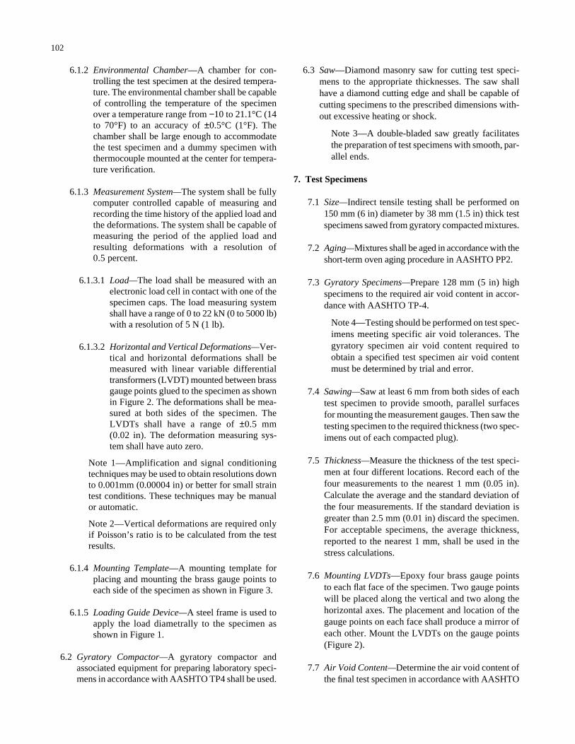
6.1.2 Environmental Chamber—A chamber for con-trolling the test specimen at the desired tempera-ture. The environmental chamber shall be capableof controlling the temperature of the specimenover a temperature range from −10 to 21.1°C (14to 70°F) to an accuracy of ±0.5°C (1°F). Thechamber shall be large enough to accommodatethe test specimen and a dummy specimen withthermocouple mounted at the center for tempera-ture verification.
6.1.3 Measurement System—The system shall be fullycomputer controlled capable of measuring andrecording the time history of the applied load andthe deformations. The system shall be capable ofmeasuring the period of the applied load andresulting deformations with a resolution of 0.5 percent.
6.1.3.1 Load—The load shall be measured with anelectronic load cell in contact with one of thespecimen caps. The load measuring systemshall have a range of 0 to 22 kN (0 to 5000 lb)with a resolution of 5 N (1 lb).
6.1.3.2 Horizontal and Vertical Deformations—Ver-tical and horizontal deformations shall bemeasured with linear variable differentialtransformers (LVDT) mounted between brassgauge points glued to the specimen as shownin Figure 2. The deformations shall be mea-sured at both sides of the specimen. TheLVDTs shall have a range of ±0.5 mm (0.02 in). The deformation measuring sys-tem shall have auto zero.
Note 1—Amplification and signal conditioningtechniques may be used to obtain resolutions downto 0.001mm (0.00004 in) or better for small straintest conditions. These techniques may be manualor automatic.
Note 2—Vertical deformations are required onlyif Poisson’s ratio is to be calculated from the testresults.
6.1.4 Mounting Template—A mounting template forplacing and mounting the brass gauge points toeach side of the specimen as shown in Figure 3.
6.1.5 Loading Guide Device—A steel frame is used toapply the load diametrally to the specimen asshown in Figure 1.
6.2 Gyratory Compactor—A gyratory compactor andassociated equipment for preparing laboratory speci-mens in accordance with AASHTO TP4 shall be used.
102
6.3 Saw—Diamond masonry saw for cutting test speci-mens to the appropriate thicknesses. The saw shallhave a diamond cutting edge and shall be capable ofcutting specimens to the prescribed dimensions with-out excessive heating or shock.
Note 3—A double-bladed saw greatly facilitatesthe preparation of test specimens with smooth, par-allel ends.
7. Test Specimens
7.1 Size—Indirect tensile testing shall be performed on150 mm (6 in) diameter by 38 mm (1.5 in) thick testspecimens sawed from gyratory compacted mixtures.
7.2 Aging—Mixtures shall be aged in accordance with theshort-term oven aging procedure in AASHTO PP2.
7.3 Gyratory Specimens—Prepare 128 mm (5 in) highspecimens to the required air void content in accor-dance with AASHTO TP-4.
Note 4—Testing should be performed on test spec-imens meeting specific air void tolerances. Thegyratory specimen air void content required toobtain a specified test specimen air void contentmust be determined by trial and error.
7.4 Sawing—Saw at least 6 mm from both sides of eachtest specimen to provide smooth, parallel surfacesfor mounting the measurement gauges. Then saw thetesting specimen to the required thickness (two spec-imens out of each compacted plug).
7.5 Thickness—Measure the thickness of the test speci-men at four different locations. Record each of thefour measurements to the nearest 1 mm (0.05 in).Calculate the average and the standard deviation ofthe four measurements. If the standard deviation isgreater than 2.5 mm (0.01 in) discard the specimen.For acceptable specimens, the average thickness,reported to the nearest 1 mm, shall be used in thestress calculations.
7.6 Mounting LVDTs—Epoxy four brass gauge pointsto each flat face of the specimen. Two gauge pointswill be placed along the vertical and two along thehorizontal axes. The placement and location of thegauge points on each face shall produce a mirror ofeach other. Mount the LVDTs on the gauge points(Figure 2).
7.7 Air Void Content—Determine the air void content ofthe final test specimen in accordance with AASHTO
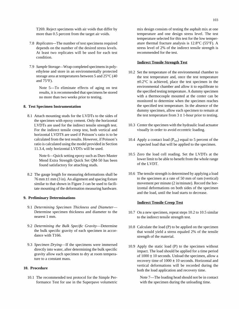
T269. Reject specimens with air voids that differ bymore than 0.5 percent from the target air voids.
7.8 Replicates—The number of test specimens requireddepends on the number of the desired stress levels.At least two replicates will be used for each testcondition.
7.9 Sample Storage—Wrap completed specimens in poly-ethylene and store in an environmentally protectedstorage area at temperatures between 5 and 25°C (40and 75°F).
Note 5—To eliminate effects of aging on testresults, it is recommended that specimens be storedno more than two weeks prior to testing.
8. Test Specimen Instrumentation
8.1 Attach mounting studs for the LVDTs to the sides ofthe specimen with epoxy cement. Only the horizontalLVDTs are used for the indirect tensile strength test.For the indirect tensile creep test, both vertical andhorizontal LVDTS are used if Poisson’s ratio is to becalculated from the test results. However, if Poisson’sratio is calculated using the model provided in Section11.3.4, only horizontal LVDTs will be used.
Note 6—Quick setting epoxy such as Duro MasterMend Extra Strength Quick Set QM-50 has beenfound satisfactory for attaching studs.
8.2 The gauge length for measuring deformations shall be76 mm ±1 mm (3 in). An alignment and spacing fixturesimilar to that shown in Figure 3 can be used to facili-tate mounting of the deformation measuring hardware.
9. Preliminary Determinations
9.1 Determining Specimen Thickness and Diameter—Determine specimen thickness and diameter to thenearest 1 mm.
9.2 Determining the Bulk Specific Gravity—Determinethe bulk specific gravity of each specimen in accor-dance with T166.
9.3 Specimen Drying—If the specimens were immerseddirectly into water, after determining the bulk specificgravity allow each specimen to dry at room tempera-ture to a constant mass.
10. Procedure
10.1 The recommended test protocol for the Simple Per-formance Test for use in the Superpave volumetric
103
mix design consists of testing the asphalt mix at onetemperature and one design stress level. The testtemperature selected for this test for the low temper-ature thermal fracture analysis is 12.8°C (55°F). Astress level of 2% of the indirect tensile strength isrecommended for the test.
Indirect Tensile Strength Test
10.2 Set the temperature of the environmental chamber tothe test temperature and, once the test temperature±0.2°C is achieved, place the test specimen in theenvironmental chamber and allow it to equilibrate tothe specified testing temperature. A dummy specimenwith a thermocouple mounted at the center can bemonitored to determine when the specimen reachesthe specified test temperature. In the absence of thedummy specimen, allow each specimen to remain atthe test temperature from 3 ± 1-hour prior to testing.
10.3 Center the specimen with the hydraulic load actuatorvisually in order to avoid eccentric loading.
10.4 Apply a contact load (Pmin) equal to 5 percent of theexpected load that will be applied to the specimen.
10.5 Zero the load cell reading. Set the LVDTs at thelower limit to be able to benefit from the whole rangeof the LVDT.
10.6 The tensile strength is determined by applying a loadto the specimen at a rate of 50 mm of ram (vertical)movement per minute (2 in/minute). Record the hor-izontal deformations on both sides of the specimenand the load, until the load starts to decrease.
Indirect Tensile Creep Test
10.7 On a new specimen, repeat steps 10.2 to 10.5 similarto the indirect tensile strength test.
10.8 Calculate the load (P) to be applied on the specimenthat would yield a stress equaled 2% of the tensilestrength of the material.
10.9 Apply the static load (P) to the specimen withoutimpact. The load should be applied for a time periodof 1000 ± 10 seconds. Unload the specimen, allow arecovery time of 1000 ± 10 seconds. Horizontal andvertical deformations will be recorded during theboth the load application and recovery time.
Note 7—The loading head should not be in contactwith the specimen during the unloading time.

Note 8—Vertical deformations are required only ifPoisson’s ratio is to be calculated from the testresults.
11. Calculations
11.1 Determine the air voids for each specimen.
11.2 Tensile Strength Calculations.
11.2.1 Determine the average thickness, diameter foreach replicate.
11.2.2 Obtain the maximum load recorded for eachreplicate.
11.2.3 Calculate the horizontal tensile strength for eachreplicate, as follows:
Where:
Pmax = maximum load on the load–deformationplot
d = diameter of specimenT = thickness of specimen.
11.2.4 Calculate the average horizontal tensile strengthof the two replicates. The two values should bewithin 15% of each other.
11.3 Creep Compliance Calculations.
11.3.1 Determine the average thickness, diameter foreach replicate.
11.3.2 Determine the average horizontal (δxx) and ver-tical (δyy) deformations from both sides of thespecimen as a function of time (t).
11.3.3 Calculate Poisson’s ratio, µ, using the verticaland horizontal deformations, as follows:
11.3.4 Or Poisson’s ratio, µ, can be determined froma regression equation developed by (Mirza &
µδ δ
δ δ=
∗ −− ∗
( . / . )( . . / )1 0695 0 23390 7801 0 3074
xx yy
xx yy
Horizontal Tensile Stress SPTdt= = 2 max
π
104
Witczak) if only horizontal LVDTs are used.The equation is:
Temperature is expressed in degree Fahrenheit.
11.3.5 Calculate the Modulus, E(t) , as follows:
11.3.6 Calculate Creep Compliance, D(t) , as a functionof time as follows:
D(t) = E(t)-1 = Dtm
Where:
D = the intercept of the creep compliance–timecurve
m = the slope of the creep compliance–time curve.
11.3.7 Fit a power model for the creep compliance ver-sus time to obtain the slope (m) and the intercept(D). Using the slope and the intercept values cal-culate the creep compliance at a time of 1000 sec-onds from the equation given in Section 11.3.6.Figure 4 shows a creep compliance versus logtime plot.
11.3.8 Calculate the average values for the creep com-pliance parameters (D and m) and the creep com-pliance at 1000 seconds from both replicates.
12. Report
12.1 Report all specimen information including mix iden-tification, storage conditions, dates of manufacturingand testing, specimen diameter and thickness, volu-metric properties, and stress level used.
12.2 Report the average horizontal tensile strength for thespecimen.
12.3 Report the average creep compliance parameters (Dand m) and the creep compliance at the end of theloading cycle (1000 seconds) by averaging the indi-rect tensile creep test results from each replicate.
Modulus E t PT xx
= = +( ) ( . . )δ
µ0 2339 0 7801
µ = ++ − ×
0 15 0 351 3 1849 0 04233
. .exp( . . )Temp
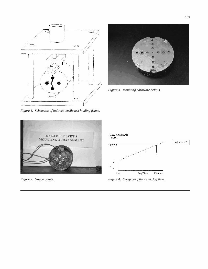
105
Figure 1. Schematic of indirect tensile test loading frame.
Figure 2. Gauge points.
Figure 3. Mounting hardware details.
Figure 4. Creep compliance vs. log time.
Abbreviations used without definitions in TRB publications:
AASHO American Association of State Highway OfficialsAASHTO American Association of State Highway and Transportation OfficialsASCE American Society of Civil EngineersASME American Society of Mechanical EngineersASTM American Society for Testing and MaterialsFAA Federal Aviation AdministrationFHWA Federal Highway AdministrationFRA Federal Railroad AdministrationFTA Federal Transit AdministrationIEEE Institute of Electrical and Electronics EngineersITE Institute of Transportation EngineersNCHRP National Cooperative Highway Research ProgramNCTRP National Cooperative Transit Research and Development ProgramNHTSA National Highway Traffic Safety AdministrationSAE Society of Automotive EngineersTCRP Transit Cooperative Research ProgramTRB Transportation Research BoardU.S.DOT United States Department of Transportation
Advisers to the Nation on Science, Engineering, and Medicine
National Academy of SciencesNational Academy of EngineeringInstitute of MedicineNational Research Council
The Transportation Research Board is a unit of the National Research Council, which serves the National Academy of Sciences and the National Academy of Engineering. The Board’s mission is to promote innovation and progress in transportation by stimulating and conducting research, facilitating the dissemination of information, and encouraging the implementation of research results. The Board’s varied activities annually draw on approximately 4,000 engineers, scientists, and other transportation researchers and practitioners from the public and private sectors and academia, all of whom contribute their expertise in the public interest. The program is supported by state transportation departments, federal agencies including the component administrations of the U.S. Department of Transportation, and other organizations and individuals interested in the development of transportation.
The National Academy of Sciences is a private, nonprofit, self-perpetuating society of distin-guished scholars engaged in scientific and engineering research, dedicated to the furtherance of science and technology and to their use for the general welfare. Upon the authority of the charter granted to it by the Congress in 1863, the Academy has a mandate that requires it to advise the federal government on scientific and technical matters. Dr. Bruce M. Alberts is president of the National Academy of Sciences.
The National Academy of Engineering was established in 1964, under the charter of the National Academy of Sciences, as a parallel organization of outstanding engineers. It is autonomous in its administration and in the selection of its members, sharing with the National Academy of Sciences the responsibility for advising the federal government. The National Academy of Engineering also sponsors engineering programs aimed at meeting national needs, encourages education and research, and recognizes the superior achievements of engineers. Dr. William A. Wulf is president of the National Academy of Engineering.
The Institute of Medicine was established in 1970 by the National Academy of Sciences to secure the services of eminent members of appropriate professions in the examination of policy matters pertaining to the health of the public. The Institute acts under the responsibility given to the National Academy of Sciences by its congressional charter to be an adviser to the federal government and, upon its own initiative, to identify issues of medical care, research, and education. Dr. Kenneth I. Shine is president of the Institute of Medicine.
The National Research Council was organized by the National Academy of Sciences in 1916 to associate the broad community of science and technology with the Academy’s purpose of furthering knowledge and advising the federal government. Functioning in accordance with general policies determined by the Academy, the Council has become the principal operating agency of both the National Academy of Sciences and the National Academy of Engineering in providing services to the government, the public, and the scientific and engineering communities. The Council is administered jointly by both the Academies and the Institute of Medicine. Dr. Bruce M. Alberts and Dr. William A. Wulf are chairman and vice chairman, respectively, of the National Research Council.


