TRANSPORTATION RESEARCH BOARD

Truck Trip Generation Data

A Synthesis of Highway Practice

NATIONALCOOPERATIVE HIGHWAYRESEARCH PROGRAMNCHRP

SYNTHESIS 298

NATIONAL RESEARCH COUNCIL

N A T I O N A L C O O P E R A T I V E H I G H W A Y R E S E A R C H P R O G R A M

NCHRP SYNTHESIS 298

Truck Trip Generation Data

A Synthesis of Highway Practice CONSULTANT

MICHAEL J. FISCHER Cambridge Systematics, Inc.

and MYONG HAN

Jack Faucett Associates

TOPIC PANEL FRANK BARON, Miami Urbanized Area Metropolitan Planning Organization

RUSSELL B. CAPELLE, JR., U.S. Department of Transportation LEE CHIMINI, Federal Highway Administration

ROBERT J. CZERNIAK, New Mexico State University TED DAHLBURG, Delaware Valley Regional Planning Commission

ALAN DANAHER, Kittelson & Associates, Inc. STEVEN R. KALE, Oregon Department of Transportation

THOMAS M. PALMERLEE, Transportation Research Board CHARLES SANFT, Minnesota Department of Transportation

ROBERT SNYDER, United Parcel Service CAROL H. WALTERS, Texas Transportation Institute

SUBJECT AREAS Planning and Administration and Highway Operations, Capacity, and Traffic Control

Research Sponsored by the American Association of State Highway and Transportation Officials in Cooperation with the Federal Highway Administration

TRANSPORTATION RESEARCH BOARD — NATIONAL RESEARCH COUNCIL

NATIONAL ACADEMY PRESS

WASHINGTON, D.C. — 2001

NATIONAL COOPERATIVE HIGHWAY RESEARCH PROGRAM Systematic, well-designed research provides the most effective approach to the solution of many problems facing highway ad-ministrators and engineers. Often, highway problems are of local interest and can best be studied by highway departments individu-ally or in cooperation with their state universities and others. How-ever, the accelerating growth of highway transportation develops increasingly complex problems of wide interest to highway au-thorities. These problems are best studied through a coordinated program of cooperative research. In recognition of these needs, the highway administrators of the American Association of State Highway and Transportation Officials initiated in 1962 an objective national highway research program employing modern scientific techniques. This program is supported on a continuing basis by funds from participating member states of the Association and it receives the full coopera-tion and support of the Federal Highway Administration, United States Department of Transportation. The Transportation Research Board of the National Research Council was requested by the Association to administer the re-search program because of the Board’s recognized objectivity and understanding of modern research practices. The Board is uniquely suited for this purpose as it maintains an extensive committee structure from which authorities on any highway transportation subject may be drawn; it possesses avenues of communication and cooperation with federal, state, and local governmental agencies, universities, and industry; its relationship to the National Research Council is an insurance of objectivity; it maintains a full-time research correlation staff of specialists in highway transportation matters to bring the findings of research directly to those who are in a position to use them. The program is developed on the basis of research needs iden-tified by chief administrators of the highway and transportation departments and by committees of AASHTO. Each year, specific areas of research needs to be included in the program are proposed to the National Research Council and the Board by the American Association of State Highway and Transportation Officials. Re-search projects to fulfill these needs are defined by the Board, and qualified research agencies are selected from those that have submitted proposals. Administration and surveillance of research contracts are the responsibilities of the National Research Coun-cil and the Transportation Research Board. The needs for highway research are many, and the National Cooperative Highway Research Program can make significant contributions to the solution of highway transportation problems of mutual concern to many responsible groups. The program, however, is intended to complement rather than to substitute for or duplicate other highway research programs. NOTE: The Transportation Research Board, the National Research Council, the Federal Highway Administration, the American Asso-ciation of State Highway and Transportation Officials, and the indi-vidual states participating in the National Cooperative Highway Re-search Program do not endorse products or manufacturers. Trade or manufacturers’ names appear herein solely because they are con-sidered essential to the object of this report.

NCHRP SYNTHESIS 298 Project 20-5 FY 1999 (Topic 31-09) ISSN 0547-5570 ISBN 0-309-06908-4 Library of Congress Control No. 2001 135527 © 2001 Transportation Research Board Price $32.00 NOTICE The project that is the subject of this report was a part of the National Co-operative Highway Research Program conducted by the Transporta-tion Research Board with the approval of the Governing Board of the Na-tional Research Council. Such approval reflects the Governing Board’s judg-ment that the program concerned is of national importance and appropriate with respect to both the purposes and resources of the Na-tional Research Council. The members of the technical committee selected to monitor this pro-ject and to review this report were chosen for recognized scholarly com-petence and with due consideration for the balance of disciplines appro-priate to the project. The opinions and conclusions expressed or implied are those of the research agency that performed the research, and, while they have been accepted as appropriate by the technical committee, they are not necessarily those of the Transportation Research Board, the Na-tional Research Council, the American Association of State Highway and Transportation Officials, or the Federal Highway Administration of the U.S. Department of Transportation. Each report is reviewed and accepted for publication by the technical committee according to procedures established and monitored by the Transportation Research Board Executive Committee and the Governing Board of the National Research Council. The National Research Council was established by the National Academy of Sciences in 1916 to associate the broad community of sci-ence and technology with the Academy’s purposes of furthering knowl-edge and of advising the Federal Government. The Council has become the principal operating agency of both the National Academy of Sciences and the National Academy of Engineering in the conduct of their services to the government, the public, and the scientific and engineering commu-nities. It is administered jointly by both Academies and the Institute of Medicine. The National Academy of Engineering and the Institute of Medicine were established in 1964 and 1970, respectively, under the charter of the National Academy of Sciences. The Transportation Research Board evolved in 1974 from the High-way Research Board, which was established in 1920. The TRB incorpo-rates all former HRB activities and also performs additional functions under a broader scope involving all modes of transportation and the inter-actions of transportation with society.

Published reports of the NATIONAL COOPERATIVE HIGHWAY RESEARCH PROGRAM are available from: Transportation Research Board National Research Council 2101 Constitution Avenue, N.W. Washington, D.C. 20418 and can be ordered through the Internet at: http://www.nationalacademies.org/trb/bookstore Printed in the United States of America

PREFACE FOREWORD By Staff Transportation Research Board

A vast storehouse of information exists on nearly every subject of concern to highway administrators and engineers. Much of this information has resulted from both research and the successful application of solutions to the problems faced by practitioners in their daily work. Because previously there has been no systematic means for compiling such useful information and making it available to the entire community, the American Asso-ciation of State Highway and Transportation Officials has, through the mechanism of the National Cooperative Highway Research Program, authorized the Transportation Re-search Board to undertake a continuing project to search out and synthesize useful knowl-edge from all available sources and to prepare documented reports on current practices in the subject areas of concern. This synthesis series reports on various practices, making specific recommendations where appropriate but without the detailed directions usually found in handbooks or de-sign manuals. Nonetheless, these documents can serve similar purposes, for each is a compendium of the best knowledge available on those measures found to be the most successful in resolving specific problems. The extent to which these reports are useful will be tempered by the user’s knowledge and experience in the particular problem area. This synthesis report will be of interest to state transportation departments and their staffs, as well as to the consultants that work with them in the areas of truck trip genera-tion. Its objective is to identify available data and to provide a balanced assessment of the state of the practice in meeting the needs for and uses of these data by transportation en-gineers, travel demand modelers, and state and federal transportation planners. The syn-thesis was accomplished through a review of recent literature and a survey of representa-tives from state transportation agencies. The data collected in the study are summarized and presented in appendices for use by practitioners. Administrators, engineers, and researchers are continually faced with highway prob-lems on which much information exists, either in the form of reports or in terms of un-documented experience and practice. Unfortunately, this information often is scattered and unevaluated and, as a consequence, in seeking solutions, full information on what has been learned about a problem frequently is not assembled. Costly research findings may go unused, valuable experience may be overlooked, and full consideration may not be given to available practices for solving or alleviating the problem. In an effort to correct this situation, a continuing NCHRP project has the objective of reporting on common highway problems and synthesizing available information. The synthesis reports from this endeavor constitute an NCHRP publication series in which various forms of relevant in-formation are assembled into single, concise documents pertaining to specific highway problems or sets of closely related problems. This report of the Transportation Research Board presents a summary of key issues that affect the collection and use of truck trip generation data. Conclusions and sugges-tions for future study are also provided.

To develop this synthesis in a comprehensive manner and to ensure inclusion of sig-nificant knowledge, the available information was assembled from numerous sources, in-cluding a large number of state highway and transportation departments. A topic panel of experts in the subject area was established to guide the author’s research in organizing and evaluating the collected data, and to review the final synthesis report. This synthesis is an immediately useful document that records the practices that were acceptable within the limitations of the knowledge available at the time of its preparation. As the processes of advancement continue, new knowledge can be expected to be added to that now at hand.

CONTENTS 1 SUMMARY 5 CHAPTER ONE INTRODUCTION Statement of the Problem, 5 Scope of the Inquiry, 6 Methodology, 6 Organization of the Report, 6 7 CHAPTER TWO KEY CONSIDERATIONS IN THE DEVELOPMENT OF TRUCK TRIP GENERATION DATA Uses of Truck Trip Generation Data, 7 Trip Purposes/Classification of Trip Generating Activities, 8 Independent Variables/Estimation Techniques, 9 Data Collection, 13 16 CHAPTER THREE REVIEW OF AVAILABLE DATA SOURCES Compendia of Trip Generation Data, 17 Engineering Studies, 19 Special Generator Studies, 21 Port and Intermodal Terminal Data Resources, 21 Vehicle-Based Travel Demand Models, 22 Commodity-Based Travel Demand Models, 28 Other Critical Data Sources, 32 33 CHAPTER FOUR CURRENT STATE OF THE PRACTICE Statewide/Metropolitan Modeling, 33 Transportation Engineering Applications, 37 Organizational Willingness to Share Data, 38 39 CHAPTER FIVE CONCLUSIONS AND RECOMMENDATIONS 41 REFERENCES 43 GLOSSARY 46 APPENDIX A QUESTIONNAIRE 52 APPENDIX B SURVEY PARTICIPANTS 53 APPENDIX C TABLES CONTAINING RELEVANT TRIP GENERATION RATES

ACKNOWLEDGMENTS Michael J. Fischer, Cambridge Systematics, Inc., Oakland, Cali-fornia, was responsible for collection of the data and preparation of the report. Myong Han, Jack Faucett Associates, Walnut Creek, Cali-fornia, assisted in the preparation of the report. Valuable assistance in the preparation of this synthesis was pro-vided by the Topic Panel, consisting of Frank Baron, Transportation Systems Specialist, Miami Urbanized Area Metropolitan Planning Organization; Russell B. Capelle, Jr., Assistant Director, Bureau of Transportation Statistics/Office of Motor Carrier Information, U.S. Department of Transportation; Lee Chimini, Freight Operations, Fed-eral Highway Administration; Robert J. Czerniak, Associate Profes-sor, Department of Geography, New Mexico State University; Ted Dahlburg, Manager, Urban Goods Program, Delaware Valley Region- al Planning Commission; Alan Danaher, Principal Engineer, Kittelson & Associates, Inc.; Steven R. Kale, Senior Planner/Economist, Ore-gon Department of Transportation; Thomas M. Palmerlee, Transpor-tation Data Specialist, Transportation Research Board; Charles Sanft,

Senior Investment Analyst, Minnesota Department of Transportation; Robert Snyder, United Parcel Service; and Carol H. Walters, Senior Research Engineer, Texas Transportation Institute. This study was managed by Donna L. Vlasak, Senior Program Officer, who worked with the consultant, the Topic Panel, and the Project 20-5 Committee in the development and review of the report. Assistance in project scope development was provided by Stephen F. Maher, P.E., Manager, Synthesis Studies. Don Tippman was responsible for editing and production. Cheryl Keith assisted in meeting logistics and distribution of the questionnaire and draft reports. Crawford F. Jencks, Manager, National Cooperative Highway Re-search Program, assisted the NCHRP 20-5 Committee and the Syn-thesis staff. Information on current practice was provided by many highway and transportation agencies. Their cooperation and assistance are appreciated.

TRUCK TRIP GENERATION DATA

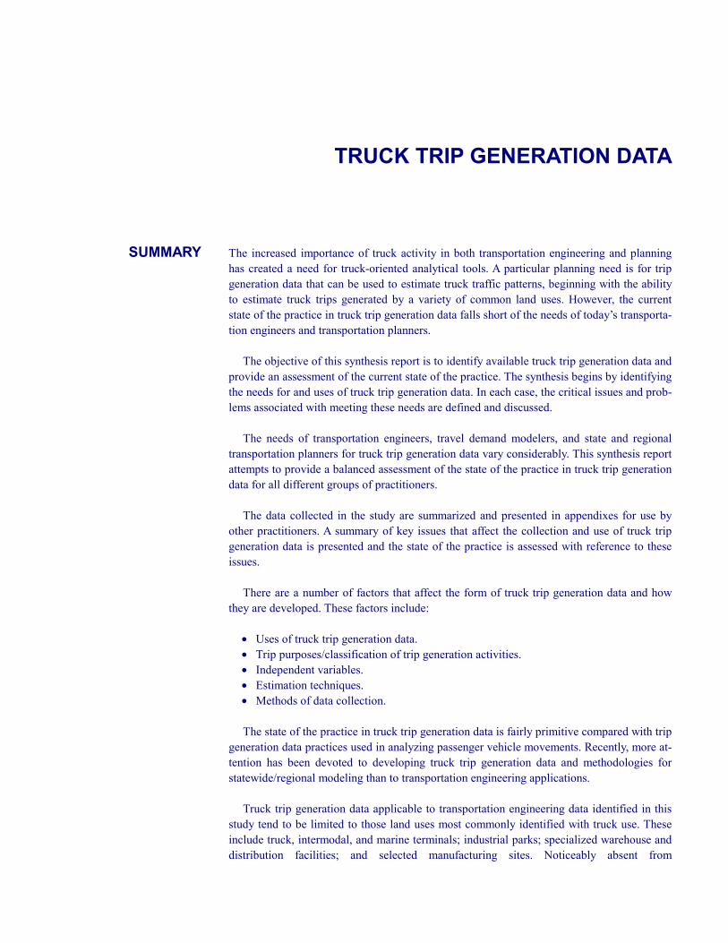
SUMMARY The increased importance of truck activity in both transportation engineering and planning

has created a need for truck-oriented analytical tools. A particular planning need is for trip generation data that can be used to estimate truck traffic patterns, beginning with the ability to estimate truck trips generated by a variety of common land uses. However, the current state of the practice in truck trip generation data falls short of the needs of today’s transporta-tion engineers and transportation planners. The objective of this synthesis report is to identify available truck trip generation data and provide an assessment of the current state of the practice. The synthesis begins by identifying the needs for and uses of truck trip generation data. In each case, the critical issues and prob-lems associated with meeting these needs are defined and discussed. The needs of transportation engineers, travel demand modelers, and state and regional transportation planners for truck trip generation data vary considerably. This synthesis report attempts to provide a balanced assessment of the state of the practice in truck trip generation data for all different groups of practitioners. The data collected in the study are summarized and presented in appendixes for use by other practitioners. A summary of key issues that affect the collection and use of truck trip generation data is presented and the state of the practice is assessed with reference to these issues. There are a number of factors that affect the form of truck trip generation data and how they are developed. These factors include:

• Uses of truck trip generation data. • Trip purposes/classification of trip generation activities. • Independent variables. • Estimation techniques. • Methods of data collection.

The state of the practice in truck trip generation data is fairly primitive compared with trip generation data practices used in analyzing passenger vehicle movements. Recently, more at-tention has been devoted to developing truck trip generation data and methodologies for statewide/regional modeling than to transportation engineering applications. Truck trip generation data applicable to transportation engineering data identified in this study tend to be limited to those land uses most commonly identified with truck use. These include truck, intermodal, and marine terminals; industrial parks; specialized warehouse and distribution facilities; and selected manufacturing sites. Noticeably absent from

2

most truck trip generation studies for engineering applications reported over the last decade are land uses such as offices, retail trade, shopping centers, and other types of commercial/ service businesses. In addition, data on truck size/configuration and vehicle dwell times are generally not available. There are two types of truck models, vehicle-based and commodity-based. Vehicle-based truck trip generation rates used in statewide and regional travel demand models are generally estimated based on land-use categories that match up well with employment by industry sec-tors corresponding to the data that metropolitan planning organizations (MPOs) typically have and/or forecast. A significant problem with this method is that these categories of land use are very broad and trip rates vary considerably within these categories from region to re-gion. Commodity-based models generally do not develop truck trip generation rates. Trip gen-eration is usually calculated by converting annual commodity tonnage data into daily truck trips using a payload conversion factor. The national Commodity Flow Survey and the Tran-search database developed by Reebie Associates are the most commonly used sources of commodity flow data, and the national Vehicle Inventory and Use Survey (VIUS) and locally collected intercept surveys are the most commonly used sources of payload data. These methods tend to underestimate trips in urban areas, because they do not account for trip chaining and local pickup and delivery activity. Most truck trip generation data include attempts to classify trucks, recognizing that differ-ent types of trucks have different missions and therefore different truck trip generation char-acteristics. Typical approaches to classifying vehicles include gross vehicle weight catego-ries, configurations (i.e., single-unit and combination vehicle), or number of axles. Unfortunately, there is little consistency from study to study, making it difficult to compare trip generation rates. In vehicle-based truck trip generation models, the most common approach to estimating trip generation rates is by land use as a function of employment. Typically, surveys are con-ducted and used to determine land use at each trip end. Expanded survey data can then be used to relate trip ends by land use (either by zone or for the region as a whole) to employ-ment corresponding to each land-use category. These models often require calibration to produce accurate results. Sources of error include the inherent variability of trip rates for ag-gregate land-use/employment categories, the inaccuracy of self-administered travel diary surveys, and the inappropriateness of employment as an explanatory variable. A number of analysts have noted that trip generation is more likely to be a function of industrial output than of employment. The relationship between output and employment (labor productivity) varies within broad industry categories, from firm to firm (often related to economies of scale), and over time. As described previously, commodity-based trip generation models generally start with an estimate of commodity flow tonnage, generally county-to-county or state-to-state flows. The annual tonnage flows are then converted to daily truck trips using payload factors. When commodity-based models are used in regional applications, the flows are typically allocated to traffic analysis zones (TAZ) using employment shares by industry/TAZ. Employment for detailed industry categories is generally difficult to obtain at the TAZ level. For vehicle-based regional modeling applications, travel diary surveys are the most fre-quently used source of data for estimating trip generation rates. This type of data collection is particularly difficult for trucking, because the owners and operators of the vehicles are

3

not always the same (leading to complicated processes for obtaining a driver’s participation), are concerned about taking time away from revenue-producing activities to fill out forms, are concerned about revealing confidential customer information, and because of growing dis-trust of government in some areas. Response rates tend to be low. In addition, obtaining a complete sampling frame including all of the vehicles that make trips within a particular modeling area can be difficult if a high percentage of trips are made by out-of-area vehicles. Truck trip generation data for transportation engineering applications is typically obtained from vehicle classification counts. Accuracy of equipment for automated counts and selec-tion of locations at which to take counts (in order to capture all traffic associated with a particular site and only traffic associated with the site) can be a challenge. Most studies re-ported in the literature calculate rates based on extremely small samples (fewer than 10 ob-servations), with high variability from site to site (as high as an order of magnitude differ-ence). Survey results suggest the following activities to help improve the collection and analysis of truck trip generation data.

• Because limited information is available on truck trip generation rates for use in trans-portation engineering applications, undertake a comprehensive and systematic data collection program to address the serious deficiencies in truck trip generation data. Ef-forts should focus on land uses such as industrial parks, manufacturing facilities, warehouses, office buildings, and various categories of service and retail industries.

• Prepare a new state of the practice manual for statewide truck trip generation modeling using commodity flow information. As part of this program, truck trip generation rates per employee at the 2-digit Standard Commodity Transportation Group level of detail from different commodity-based state models might be compared to determine if such rates might be transferable from one state to another. Another important area of re-search supporting commodity-based models would be to improve data on average pay-loads for conversion of tonnage flows to truck trips and for estimating axle loadings in order to support pavement design initiatives.

• A rethinking of the VIUS survey to redefine “major commodity” to agree with the SCTG system and “sample size” to provide sufficient samples by strata to meet the commodity-based models’ disaggregation requirements by commodity and truck size.

• Collect data from external roadside intercepts to identify the number of internal trips typically made by trucks registered outside of a region.

• Conduct research to estimate the commodity distribution practices of different in-dustries.

• Compile truck trip generation data and re-estimation of trip rates in a constant manner to determine how variable these rates are.

In the future, it is likely that some MPOs will continue to experiment with commodity-based trip generation models. The utility of commodity-based models could be further ex-tended if additional research is conducted to estimate the commodity distribution practices of different industries. Commodity-based models provide little information about the various reload distribution movements between the initial production and end-user consumption trip ends, which results in an underestimation of trips. Further investigation is needed to deter-mine if trip generation relationships that capture these intermediate moves can be estimated.

5

CHAPTER ONE

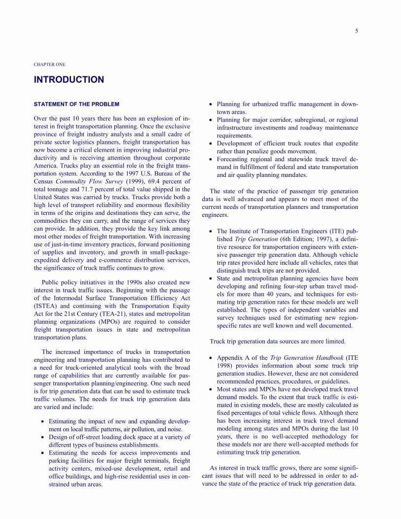
INTRODUCTION STATEMENT OF THE PROBLEM Over the past 10 years there has been an explosion of in-terest in freight transportation planning. Once the exclusive province of freight industry analysts and a small cadre of private sector logistics planners, freight transportation has now become a critical element in improving industrial pro-ductivity and is receiving attention throughout corporate America. Trucks play an essential role in the freight trans-portation system. According to the 1997 U.S. Bureau of the Census Commodity Flow Survey (1999), 69.4 percent of total tonnage and 71.7 percent of total value shipped in the United States was carried by trucks. Trucks provide both a high level of transport reliability and enormous flexibility in terms of the origins and destinations they can serve, the commodities they can carry, and the range of services they can provide. In addition, they provide the key link among most other modes of freight transportation. With increasing use of just-in-time inventory practices, forward positioning of supplies and inventory, and growth in small-package-expedited delivery and e-commerce distribution services, the significance of truck traffic continues to grow. Public policy initiatives in the 1990s also created new interest in truck traffic issues. Beginning with the passage of the Intermodal Surface Transportation Efficiency Act (ISTEA) and continuing with the Transportation Equity Act for the 21st Century (TEA-21), states and metropolitan planning organizations (MPOs) are required to consider freight transportation issues in state and metropolitan transportation plans. The increased importance of trucks in transportation engineering and transportation planning has contributed to a need for truck-oriented analytical tools with the broad range of capabilities that are currently available for pas-senger transportation planning/engineering. One such need is for trip generation data that can be used to estimate truck traffic volumes. The needs for truck trip generation data are varied and include:

• Estimating the impact of new and expanding develop-ment on local traffic patterns, air pollution, and noise.

• Design of off-street loading dock space at a variety of different types of business establishments.

• Estimating the needs for access improvements and parking facilities for major freight terminals, freight activity centers, mixed-use development, retail and office buildings, and high-rise residential uses in con-strained urban areas.

• Planning for urbanized traffic management in down-town areas.

• Planning for major corridor, subregional, or regional infrastructure investments and roadway maintenance requirements.

• Development of efficient truck routes that expedite rather than penalize goods movement.

• Forecasting regional and statewide truck travel de-mand in fulfillment of federal and state transportation and air quality planning mandates.

The state of the practice of passenger trip generation data is well advanced and appears to meet most of the current needs of transportation planners and transportation engineers.

• The Institute of Transportation Engineers (ITE) pub-lished Trip Generation (6th Edition; 1997), a defini-tive resource for transportation engineers with exten-sive passenger trip generation data. Although vehicle trip rates provided here include all vehicles, rates that distinguish truck trips are not provided.

• State and metropolitan planning agencies have been developing and refining four-step urban travel mod-els for more than 40 years, and techniques for esti-mating trip generation rates for these models are well established. The types of independent variables and survey techniques used for estimating new region-specific rates are well known and well documented.

Truck trip generation data sources are more limited.

• Appendix A of the Trip Generation Handbook (ITE 1998) provides information about some truck trip generation studies. However, these are not considered recommended practices, procedures, or guidelines.

• Most states and MPOs have not developed truck travel demand models. To the extent that truck traffic is esti-mated in existing models, these are mostly calculated as fixed percentages of total vehicle flows. Although there has been increasing interest in truck travel demand modeling among states and MPOs during the last 10 years, there is no well-accepted methodology for these models nor are there well-accepted methods for estimating truck trip generation.

As interest in truck traffic grows, there are some signifi-cant issues that will need to be addressed in order to ad-vance the state of the practice of truck trip generation data.

6

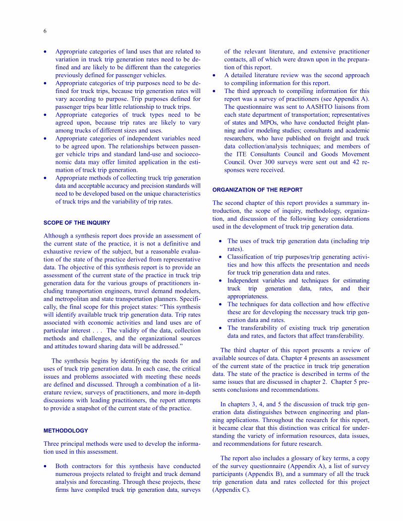
• Appropriate categories of land uses that are related to variation in truck trip generation rates need to be de-fined and are likely to be different than the categories previously defined for passenger vehicles.

• Appropriate categories of trip purposes need to be de-fined for truck trips, because trip generation rates will vary according to purpose. Trip purposes defined for passenger trips bear little relationship to truck trips.

• Appropriate categories of truck types need to be agreed upon, because trip rates are likely to vary among trucks of different sizes and uses.

• Appropriate categories of independent variables need to be agreed upon. The relationships between passen-ger vehicle trips and standard land-use and socioeco-nomic data may offer limited application in the esti-mation of truck trip generation.

• Appropriate methods of collecting truck trip generation data and acceptable accuracy and precision standards will need to be developed based on the unique characteristics of truck trips and the variability of trip rates.

SCOPE OF THE INQUIRY Although a synthesis report does provide an assessment of the current state of the practice, it is not a definitive and exhaustive review of the subject, but a reasonable evalua-tion of the state of the practice derived from representative data. The objective of this synthesis report is to provide an assessment of the current state of the practice in truck trip generation data for the various groups of practitioners in-cluding transportation engineers, travel demand modelers, and metropolitan and state transportation planners. Specifi-cally, the final scope for this project states: “This synthesis will identify available truck trip generation data. Trip rates associated with economic activities and land uses are of particular interest . . . The validity of the data, collection methods and challenges, and the organizational sources and attitudes toward sharing data will be addressed.” The synthesis begins by identifying the needs for and uses of truck trip generation data. In each case, the critical issues and problems associated with meeting these needs are defined and discussed. Through a combination of a lit-erature review, surveys of practitioners, and more in-depth discussions with leading practitioners, the report attempts to provide a snapshot of the current state of the practice. METHODOLOGY Three principal methods were used to develop the informa-tion used in this assessment. • Both contractors for this synthesis have conducted

numerous projects related to freight and truck demand analysis and forecasting. Through these projects, these firms have compiled truck trip generation data, surveys

of the relevant literature, and extensive practitioner contacts, all of which were drawn upon in the prepara-tion of this report.

• A detailed literature review was the second approach to compiling information for this report.

• The third approach to compiling information for this report was a survey of practitioners (see Appendix A). The questionnaire was sent to AASHTO liaisons from each state department of transportation; representatives of states and MPOs, who have conducted freight plan-ning and/or modeling studies; consultants and academic researchers, who have published on freight and truck data collection/analysis techniques; and members of the ITE Consultants Council and Goods Movement Council. Over 300 surveys were sent out and 42 re-sponses were received.

ORGANIZATION OF THE REPORT The second chapter of this report provides a summary in-troduction, the scope of inquiry, methodology, organiza-tion, and discussion of the following key considerations used in the development of truck trip generation data.

• The uses of truck trip generation data (including trip rates).

• Classification of trip purposes/trip generating activi-ties and how this affects the presentation and needs for truck trip generation data and rates.

• Independent variables and techniques for estimating truck trip generation data, rates, and their appropriateness.

• The techniques for data collection and how effective these are for developing the necessary truck trip gen-eration data and rates.

• The transferability of existing truck trip generation data and rates, and factors that affect transferability.

The third chapter of this report presents a review of available sources of data. Chapter 4 presents an assessment of the current state of the practice in truck trip generation data. The state of the practice is described in terms of the same issues that are discussed in chapter 2. Chapter 5 pre-sents conclusions and recommendations. In chapters 3, 4, and 5 the discussion of truck trip gen-eration data distinguishes between engineering and plan-ning applications. Throughout the research for this report, it became clear that this distinction was critical for under-standing the variety of information resources, data issues, and recommendations for future research. The report also includes a glossary of key terms, a copy of the survey questionnaire (Appendix A), a list of survey participants (Appendix B), and a summary of all the truck trip generation data and rates collected for this project (Appendix C).

7

CHAPTER TWO KEY CONSIDERATIONS IN THE DEVELOPMENT OF TRUCK TRIP GENERATION DATA To appreciate the current state of the practice of truck trip generation data it is necessary to understand a number of fundamental topics associated with the application of truck trip generation rates, the estimation of truck trip generation rates/models, and the collection of truck trip generation data. These topics are outlined in this chapter. USES OF TRUCK TRIP GENERATION DATA The uses of truck trip generation data can be broadly clas-sified in two major categories: (1) transportation engineer-ing applications, and (2) statewide, regional, and subre-gional planning applications. Each of these categories of truck trip generation data applications creates different needs with respect to classification of trip purposes, level of land use and industrial detail, and classification of truck types. A clear statement of the need for and potential appli-cations of truck trip generation data for transportation en-gineering and planning practice is provided here. Transportation Engineering Applications

• Uses – Traffic impact fee assessment – Traffic operation studies – Site impact analysis – Street design – Provision of off-street and on-street loading facilities – Provision of off-street and on-street parking

• Issues

– Requires high level of accuracy for wide range of land-use types

– Requires accuracy at microscale level – Trip rates must be highly transferable – Clear and consistent procedures for estimating

rates and presenting the data are needed Statewide, Regional, and Subregional Planning Applications

• Uses – Travel demand modeling – Development of state, regional, and local trans-

portation plans – Evaluation of transportation improvement program

projects – Identification of system operational deficiencies

and evaluation of improvements

– Corridor studies and plans – Activity inputs to air quality analysis programs – Intermodal access studies

• Issues

– Widely varying levels of geographic detail – Widely varying levels of precision of estimate

required – Transferability of results – Compatibility of rates and socioeconomic and/or

land-use data The potential needs for reasonably accurate estimates of truck trips for engineering applications fall into three gen-eral categories: traffic operations, street and road design, and public and political concerns (ITE 1998). Transportation engineering applications of trip genera-tion data require very accurate estimates of trip generation for a wide range of land-use types. These rates must be ac-curate at the microscale because they are used to design lo-cal streets, designate or revise truck routes, estimate traffic impacts and design mitigations, assess traffic impact fees, and regulate provision of off-street loading space. The trip generation rates developed for these applications also need to be widely transferable. Clear and consistent procedures for the collection of trip generation data and the estimation and presentation of trip rates must be developed. Statewide, metropolitan, and subregional planning ap-plications of truck trip generation data are generally asso-ciated with the estimation and use of travel demand mod-els. These models are used for

• Development of state and metropolitan transportation plans;

• Evaluation of transportation improvement program projects;

• Identification of system operational deficiencies and evaluation of the traffic benefits of improvements;

• Conducting corridor studies; • Identification and evaluation of National Highway

System connector needs; and • Development of activity inputs to air quality analysis

programs. Each of these applications requires different levels of geographic detail and accuracy.

8

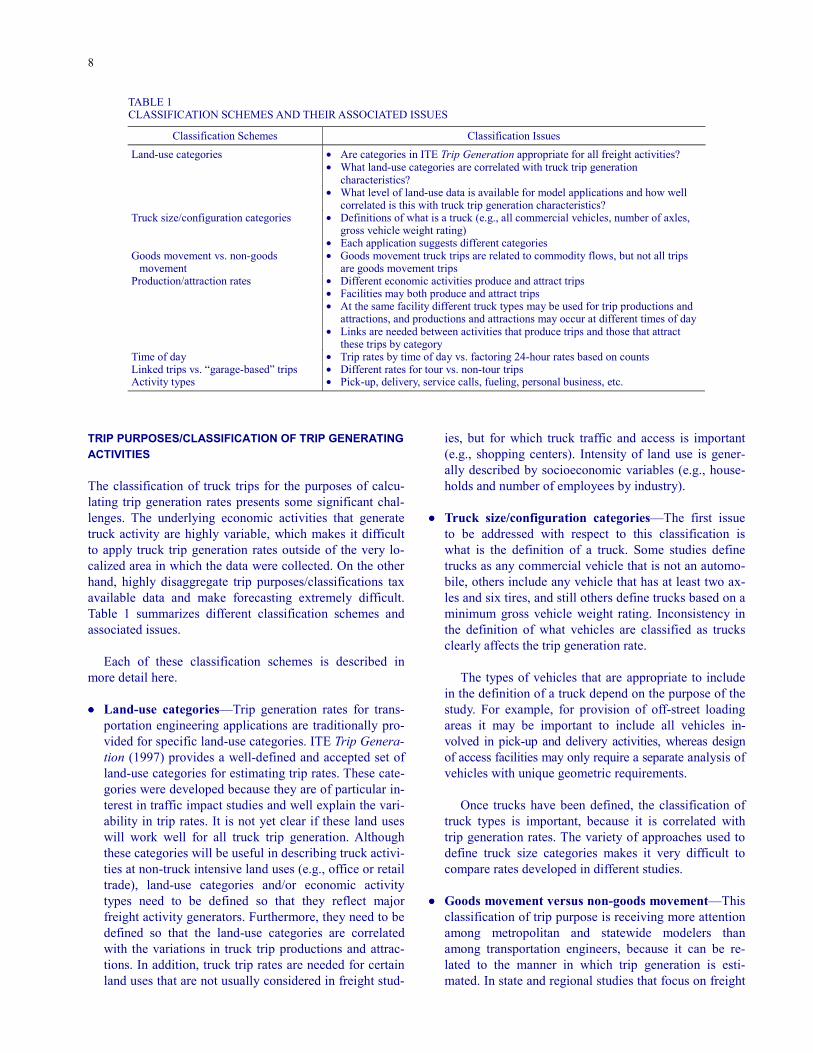
TABLE 1 CLASSIFICATION SCHEMES AND THEIR ASSOCIATED ISSUES

Classification Schemes Classification Issues Land-use categories • Are categories in ITE Trip Generation appropriate for all freight activities? • What land-use categories are correlated with truck trip generation

characteristics? • What level of land-use data is available for model applications and how well

correlated is this with truck trip generation characteristics? Truck size/configuration categories • Definitions of what is a truck (e.g., all commercial vehicles, number of axles,

gross vehicle weight rating) • Each application suggests different categories Goods movement vs. non-goods

movement • Goods movement truck trips are related to commodity flows, but not all trips

are goods movement trips Production/attraction rates • Different economic activities produce and attract trips • Facilities may both produce and attract trips • At the same facility different truck types may be used for trip productions and

attractions, and productions and attractions may occur at different times of day • Links are needed between activities that produce trips and those that attract

these trips by category Time of day • Trip rates by time of day vs. factoring 24-hour rates based on counts Linked trips vs. “garage-based” trips • Different rates for tour vs. non-tour trips Activity types • Pick-up, delivery, service calls, fueling, personal business, etc.

TRIP PURPOSES/CLASSIFICATION OF TRIP GENERATING ACTIVITIES The classification of truck trips for the purposes of calcu-lating trip generation rates presents some significant chal-lenges. The underlying economic activities that generate truck activity are highly variable, which makes it difficult to apply truck trip generation rates outside of the very lo-calized area in which the data were collected. On the other hand, highly disaggregate trip purposes/classifications tax available data and make forecasting extremely difficult. Table 1 summarizes different classification schemes and associated issues. Each of these classification schemes is described in more detail here. •••• Land-use categories—Trip generation rates for trans-

portation engineering applications are traditionally pro-vided for specific land-use categories. ITE Trip Genera-tion (1997) provides a well-defined and accepted set of land-use categories for estimating trip rates. These cate-gories were developed because they are of particular in-terest in traffic impact studies and well explain the vari-ability in trip rates. It is not yet clear if these land uses will work well for all truck trip generation. Although these categories will be useful in describing truck activi-ties at non-truck intensive land uses (e.g., office or retail trade), land-use categories and/or economic activity types need to be defined so that they reflect major freight activity generators. Furthermore, they need to be defined so that the land-use categories are correlated with the variations in truck trip productions and attrac-tions. In addition, truck trip rates are needed for certain land uses that are not usually considered in freight stud-

ies, but for which truck traffic and access is important (e.g., shopping centers). Intensity of land use is gener-ally described by socioeconomic variables (e.g., house-holds and number of employees by industry).

•••• Truck size/configuration categories—The first issue

to be addressed with respect to this classification is what is the definition of a truck. Some studies define trucks as any commercial vehicle that is not an automo-bile, others include any vehicle that has at least two ax-les and six tires, and still others define trucks based on a minimum gross vehicle weight rating. Inconsistency in the definition of what vehicles are classified as trucks clearly affects the trip generation rate.

The types of vehicles that are appropriate to include in the definition of a truck depend on the purpose of the study. For example, for provision of off-street loading areas it may be important to include all vehicles in-volved in pick-up and delivery activities, whereas design of access facilities may only require a separate analysis of vehicles with unique geometric requirements.

Once trucks have been defined, the classification of truck types is important, because it is correlated with trip generation rates. The variety of approaches used to define truck size categories makes it very difficult to compare rates developed in different studies.

•••• Goods movement versus non-goods movement—This

classification of trip purpose is receiving more attention among metropolitan and statewide modelers than among transportation engineers, because it can be re-lated to the manner in which trip generation is esti-mated. In state and regional studies that focus on freight

9

and goods movement transportation there is a growing interest in looking at commodities moved as a means for estimating the number and type of truck trips that are generated. However, when the results of these mod-eling approaches are compared to actual highway truck volumes, the estimates often fall short of the observed counts. To some extent this can be traced to the exclu-sion of truck trips related to construction, service, and utility applications that are not involved in goods movement; incomplete consideration of empty trucks; and the lack of methods for including trips in multistop tours. Methods for estimating the generation of these latter types of trips, distinct from commodity-based trip generation rate estimation methodologies, are still evolving.

•••• Production/attraction rates—Transportation engineers

and travel demand modelers are interested in distin-guishing between trip production rates and trip attrac-tion rates. In transportation engineering applications it is important to understand that for truck trips, different types of activities tend to initiate trips at a location than those activities that attract trips. For truck trips, this is more easily understood in terms of inbound trips versus outbound trips. For example, at a manufacturing facility supplies and services constitute inbound truck trips, whereas shipments of product constitute outbound truck trips. The rate at which trucks arrive inbound is very different from the rate at which they leave with out-bound shipments. In addition, the types of trucks mak-ing inbound trips may be very different from those mak-ing outbound trips. All of these factors can affect the traffic impacts that a facility will have on adjacent roadways and communities.

Similar concerns relate to travel demand modeling because the approaches and rates used to estimate trip productions and attractions may be different. For exam-ple, it is rare that manufacturers will ship their products directly to households. However, if manufacturer pro-ductions and household attractions are not distinguished in a model, this type of unlikely distribution pattern can result in the model.

•••• Time of day—In many applications of truck trip gen-

eration data, the time of day distribution of the trips is very important. For example, understanding the varia-tion in truck traffic as it relates to peak versus off-peak traffic conditions is often important. In many transporta-tion engineering applications, these time-of-day charac-teristics are resolved by estimating different trip genera-tion rates for different times of the day. In most current truck travel demand models the approach is to estimate 24-hour trip generation rates and to then factor the re-sulting traffic assignment volumes into time periods based on ground counts from different time periods.

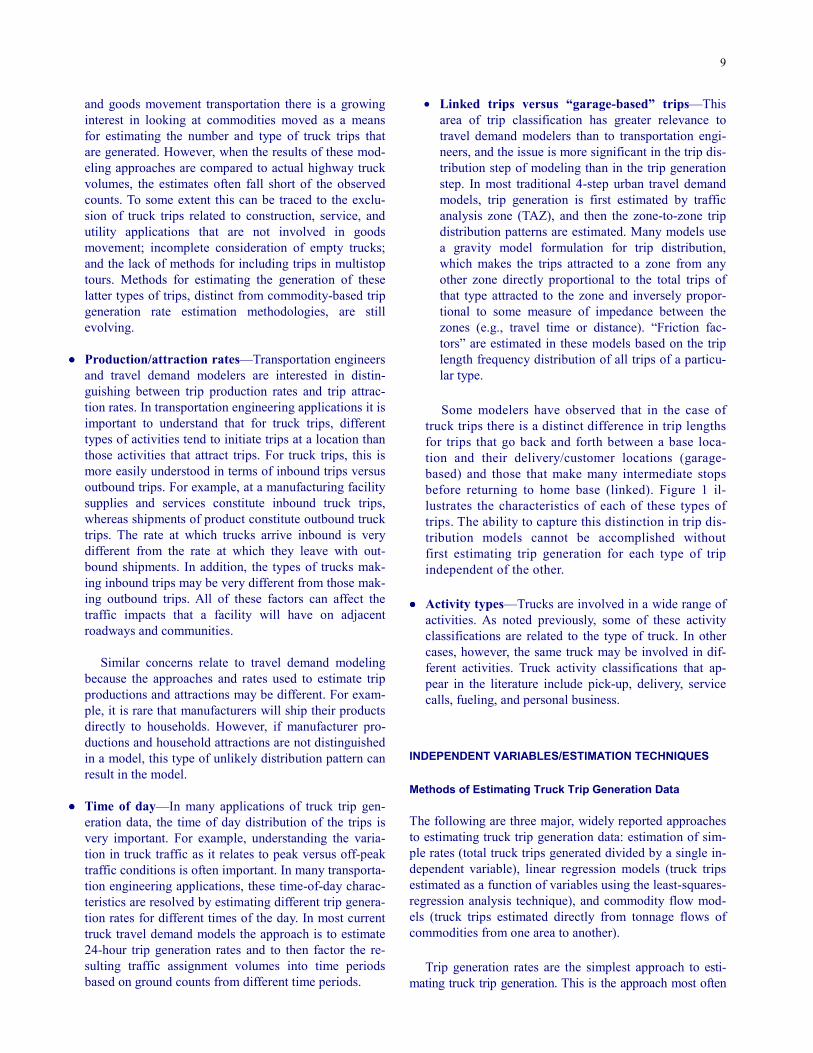
• Linked trips versus “garage-based” trips—This area of trip classification has greater relevance to travel demand modelers than to transportation engi-neers, and the issue is more significant in the trip dis-tribution step of modeling than in the trip generation step. In most traditional 4-step urban travel demand models, trip generation is first estimated by traffic analysis zone (TAZ), and then the zone-to-zone trip distribution patterns are estimated. Many models use a gravity model formulation for trip distribution, which makes the trips attracted to a zone from any other zone directly proportional to the total trips of that type attracted to the zone and inversely propor-tional to some measure of impedance between the zones (e.g., travel time or distance). “Friction fac-tors” are estimated in these models based on the trip length frequency distribution of all trips of a particu-lar type.

Some modelers have observed that in the case of truck trips there is a distinct difference in trip lengths for trips that go back and forth between a base loca-tion and their delivery/customer locations (garage-based) and those that make many intermediate stops before returning to home base (linked). Figure 1 il-lustrates the characteristics of each of these types of trips. The ability to capture this distinction in trip dis-tribution models cannot be accomplished without first estimating trip generation for each type of trip independent of the other.

•••• Activity types—Trucks are involved in a wide range of

activities. As noted previously, some of these activity classifications are related to the type of truck. In other cases, however, the same truck may be involved in dif-ferent activities. Truck activity classifications that ap-pear in the literature include pick-up, delivery, service calls, fueling, and personal business.

INDEPENDENT VARIABLES/ESTIMATION TECHNIQUES Methods of Estimating Truck Trip Generation Data The following are three major, widely reported approaches to estimating truck trip generation data: estimation of sim-ple rates (total truck trips generated divided by a single in-dependent variable), linear regression models (truck trips estimated as a function of variables using the least-squares-regression analysis technique), and commodity flow mod-els (truck trips estimated directly from tonnage flows of commodities from one area to another). Trip generation rates are the simplest approach to esti-mating truck trip generation. This is the approach most often

10

“Garage-based” Trip Trip Attraction

Trip Production Example: Factory truckload delivery to a distribution center. Note: Each production–attraction represents two mirror-image trips. Linked Trips Trip Attraction #1 Trip Attraction #2 Trip Production Trip Attraction #3 Example: United Parcel Service pick-up and delivery routes. Note: Each attraction site is the origin for a trip produced at a distant site—how to link all the trips in a chain during trip distribution? Does this require a different approach for trip generation?

FIGURE 1 “Garage-based” versus linked trips.

used in transportation engineering applications. It has also been used extensively for travel demand modeling ap-plications. The general approach is to select land-use categories and estimate trip generation rates for each category as a function of a single independent variable that measures the intensity of land use or activity at the land use. Typical examples of independent variables used include

• Acreage of land used, • Square feet of building floor area, and • Employment or activity indicators (e.g., number of

container lifts, import/export container moves).

As noted previously, the selection of land-use categories is a critical question and one for which little guidance is available. The general approach in modeling applications is to use land-use categories that correspond closely to indus-try/employment categories, which are forecast at the zonal level in regional socioeconomic models. This presents se-rious limitations. In the best cases, these may include 10–12 categories that correspond to major industry groups in the North American Industrial Classification System (NAICS), which recently replaced the Standard Industrial Classification (SIC) system as the preferred system for classifying industries. Trip rates estimated at the major in-dustry level of detail (i.e., 10–12 categories) are not only

11

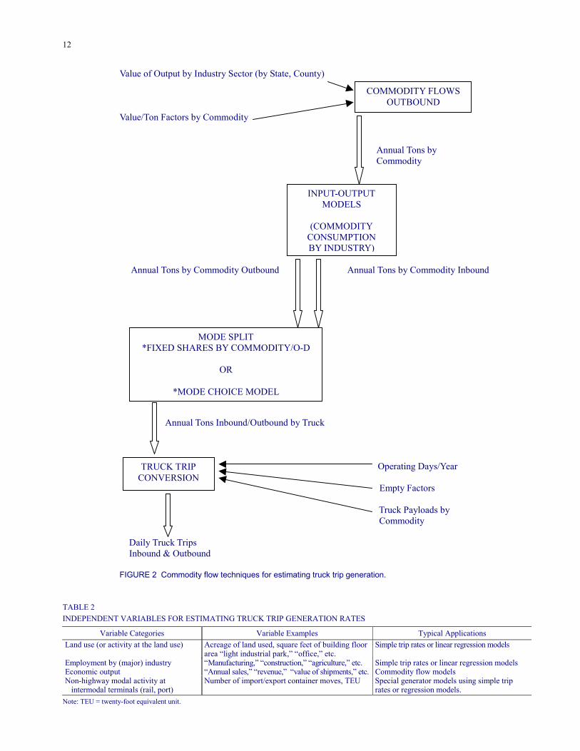
highly variable from one region to another, but may even vary significantly within regions. Some regional travel demand models attempt to solve this problem by estimat-ing different subregional trip generation rates for the same land-use category. Another common approach used to deal with this prob-lem in regional models is to identify “special generators,” which are responsible for significant truck activity and for whom the regional trip rates would either over- or underes-timate trip generation. Clearly, this problem demonstrates the lack of interregional transferability of results estimated using this type of approach at this level of detail. Linear regression models have much in common with simple trip rate estimation, although the method for calcu-lating the rates differs. In transportation engineering appli-cations, the ITE has established a standard format for pre-senting results estimated with regression models. In this application, trip generation volumes are estimated for many different sites in the same land-use category. The re-gression model attempts to fit a straight line to the data and the slope of the line represents the constant trip generation rate. Regression models are also used to estimate regional and statewide trip generation. These models generally es-timate the number of trips generated in large zones, or dis-tricts, based on the expansion of survey data. Trips are then regressed against an independent variable or variables measuring activity levels in each zone or district. These models can be developed individually for each land-use type or a single model can be developed with multiple in-dependent variables representing the different activities in the zone (e.g., different employment variables). Regression models are often used in regional studies when the survey data collected for truck trips do not include valid classifica-tions of land use at each trip end. The regression models suffer from most of the same problems identified previ-ously for simple trip rates. Commodity flow techniques for estimating truck trip generation are relatively new approaches and do not seem to be applicable to transportation engineering applications. First proposed for statewide modeling applications (Mem-mott 1983), this approach is beginning to be applied in metropolitan models and corridor studies as well. The basic approach (see Figure 2) is to use economic data and forecasts of industrial output and consumer final demand along with economic input–output models to esti-mate annual production and consumption of goods. Data from sources such as the U.S. Economic Census provide much of the information needed to make these estimates on a state-by-state basis and local employment data are then often used to disaggregate state level production and

consumption estimates to more disaggregate zones (coun-ties, cities, or TAZs). The origin–destination patterns of the flows are developed from a variety of data sources includ-ing the U.S. Commodity Flow Survey (CFS), locally con-ducted origin–destination surveys, and estimates from cali-brated gravity models. Because most of the economic data and models used to estimate production and consumption of goods is measured in value (dollars), they must first be converted to tonnage of shipments (using value-to-weight ratios derived from various public and private proprietary sources), then split by freight mode (often using fixed modal shares by com-modity and origin–destination pair based on data such as the CFS), and finally converted to truck trips. This last step is the critical link to traditional truck trip generation data and is the subject of some controversy. Many studies con-vert tonnage flows into truck trips using average payload factors. These payload factors may come from local sur-veys or from national data, such as the Vehicle Inventory and Use Survey (VIUS). VIUS is a truck survey conducted every 5 years by the U.S. Bureau of the Census as part of the Economic Census. The survey collects extensive data about equipment and activity characteristics of the nation’s truck fleets. The degree of disaggregation of commodities in the data used to estimate average payloads will ultimately influence the accuracy of results and often suffers from the same data aggregation problems described previously for trip rates and regression models. Critics of this approach to es-timating truck traffic also note that the commodity flow and payload data tend to neglect the many local pick-up and delivery trips that constitute the majority of truck trips within urban areas. These local trips also include many non-goods movement trips that are not estimated in com-modity flow models. Another important element of truck trip generation that must be addressed in commodity flow models is the esti-mation of empty truck trips, which are not accounted for in the production–consumption estimation techniques and must, therefore, be added at the truck trip conversion step. Choice of Independent Variables Table 2 summarizes different variable categories used for estimating truck trip generation rates. The previous discussion indicated that in most cases where trip rates or regression models are used to estimate truck trip generation, the independent variables used will either be land-use variables (i.e., building floor area or acres of land used) or employment variables. Although these variables may be appropriate for estimating truck trip

12

Value of Output by Industry Sector (by State, County) Value/Ton Factors by Commodity Annual Tons by Commodity Annual Tons by Commodity Outbound Annual Tons by Commodity Inbound Annual Tons Inbound/Outbound by Truck Operating Days/Year Empty Factors Truck Payloads by Commodity Daily Truck Trips Inbound & Outbound FIGURE 2 Commodity flow techniques for estimating truck trip generation. TABLE 2 INDEPENDENT VARIABLES FOR ESTIMATING TRUCK TRIP GENERATION RATES

Variable Categories Variable Examples Typical Applications Land use (or activity at the land use)

Acreage of land used, square feet of building floor area “light industrial park,” “office,” etc.

Simple trip rates or linear regression models

Employment by (major) industry “Manufacturing,” “construction,” “agriculture,” etc. Simple trip rates or linear regression models Economic output “Annual sales,” “revenue,” “value of shipments,” etc. Commodity flow models Non-highway modal activity at intermodal terminals (rail, port)

Number of import/export container moves, TEU Special generator models using simple trip rates or regression models.

Note: TEU = twenty-foot equivalent unit.

COMMODITY FLOWS OUTBOUND

INPUT-OUTPUT MODELS

(COMMODITY

CONSUMPTION BY INDUSTRY)

TRUCK TRIP CONVERSION

MODE SPLIT *FIXED SHARES BY COMMODITY/O-D

OR

*MODE CHOICE MODEL

13

attraction, there is considerable debate as to the effective-ness of these variables in estimating truck trip production. The source of this concern can be traced to industrial pro-duction function and factor productivity issues and is most clearly illustrated through discussion of the use of em-ployment as a predictor of truck trips. Each industry uses factor inputs differently to produce a unit of output, and the relationship between inputs and outputs is described in a production function. Labor, being a factor of production, is one of these inputs, and there is a distinct relationship between output and employment for each industry. If output is thought of as a measure of goods that need to be shipped from a place of production, then it is clearly related to truck trip generation and the relation-ship between employment and output is the basis for the relationship between employment and truck trips. Eco-nomic data clearly demonstrate that labor productivity var-ies substantially from industry to industry. Therefore, if employment is to be used to estimate truck trip generation, the industry/land-use categories may need to be very dis-aggregate in order to produce accurate results. This prob-lem may even exist from business to business within a par-ticular industry. It is well-documented that some production processes exhibit economies of scale. In these cases we would expect to see different truck trip generation rates per employee for large businesses than for small businesses. A final problem with employment as a predictor of truck trips is that labor productivity for a given industry changes over time. A very significant issue for freight fore-casting is that manufacturing employment in the United States over the last 20 years has remained relatively flat, while manufacturing output, and associated freight trans-portation demand, has experienced healthy growth (U.S. Bureau of the Census, Commodity Flow Survey 1999; U.S. Bureau of the Census, Economic Census 1999). Clearly, using a constant trip generation rate based on employment could result in a gross underestimation of future truck trips if productivity improvement is not taken into account. Commodity flow models attempt to circumvent this prob-lem by using economic models of production and con-sumption of goods to estimate truck trips. There is a new class of special generator models being developed that bears mention here, because the types of independent variables they use are somewhat unique. This type of model has seen the greatest recent application at container ports. In these models, truck trips through a port or intermodal terminal gate will be estimated as a function of the non-truck mode activity. For example, truck trips at a container port may be estimated as a function of import–export Twenty-Foot Equivalent Unit (TEU) throughputs on the wharfside. [TEU is a commonly accepted measure of container traffic and derives from the original containers

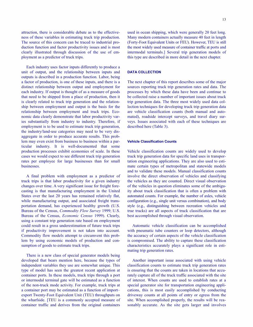
used in ocean shipping, which were generally 20 feet long. Many modern containers actually measure 40 feet in length (Forty-Foot Equivalent Units or FEU). However, TEU is still the most widely used measure of container traffic at ports and intermodal terminals.] Several trip generation models of this type are described in more detail in the next chapter. DATA COLLECTION The next chapter of this report describes some of the major sources reporting truck trip generation rates and data. The processes by which these data have been and continue to be collected raise a number of important issues about truck trip generation data. The three most widely used data col-lection techniques for developing truck trip generation data are vehicle classification counts (both manual and auto-mated), roadside intercept surveys, and travel diary sur-veys. Issues associated with each of these techniques are described here (Table 3). Vehicle Classification Counts Vehicle classification counts are widely used to develop truck trip generation data for specific land uses in transpor-tation engineering applications. They are also used to esti-mate certain types of metropolitan and statewide models and to validate these models. Manual classification counts involve the direct observation of vehicles and classifying the vehicles as they are counted. Direct visual observation of the vehicles in question eliminates some of the ambigu-ity about truck classification that is often a problem with automated counts. For example, the number of axles, vehicle configuration (e.g., single unit versus combination), and body style (e.g., distinguishing between recreation vehicles and true trucks) are all aspects of truck classification that are best accomplished through visual observation. Automatic vehicle classification can be accomplished with pneumatic tube counters or loop detectors, although the accuracy of certain aspects of the vehicle classification is compromised. The ability to capture these classification characteristics accurately plays a significant role in esti-mating trip generation rates. Another important issue associated with using vehicle classification counts to estimate truck trip generation rates is ensuring that the counts are taken in locations that accu-rately capture all of the truck traffic associated with the site of interest. When counts are used to establish rates at a special generator site for transportation engineering appli-cations, this is most easily accomplished by conducting driveway counts at all points of entry or egress from the site. When accomplished properly, the results will be rea-sonably accurate. As the site gets larger and involves

14

TABLE 3 TRUCK TRIP GENERATION DATA COLLECTION METHODS

Method Characteristics

Vehicle classification counts • Used most frequently for trip rates to support engineering analysis • Manual counts provide more flexibility in setting classification categories and may eliminate some

ambiguity • Automatic counts may be less expensive, but accuracy of equipment is a concern • Count locations must be chosen to capture all relevant traffic, but to eliminate background traffic • All traffic can be counted Roadside intercept surveys • Usually involves sampling • Locations must be selected where traffic can be safely intercepted • Data on land-use characteristics and trip purpose can also be collected and correlated with trip

generation • Payload factors, day-of-week distributions, and time-of-day distributions can be collected for

commodity flow models • Expansion of partial day data to 24-hour trip rates is an issue Travel diary surveys • Used most frequently to support travel demand models • Good sampling frames with complete truck population are often unavailable • Expansion of data must account for out-of-service vehicles • Underreporting of trips is a problem • Truck trip diary surveys have very low response rates and may be subject to non-response bias

internal circulation, as it may in an industrial park or air-port, this type of data collection can become more difficult. Roadside Intercept Surveys Roadside intercept surveys are often used to develop truck trip generation data for metropolitan and statewide models. Intercept surveys have many of the benefits of vehicle classification counts (if appropriate sites can be identified) and are often conducted simultaneously with classification counts. The advantage of the intercept survey is that it can be used to collect trip information that can be used in other aspects of metropolitan modeling. The primary problem associated with intercept surveys is that they are difficult and costly to conduct, and it is frequently impossible to find locations where traffic can be properly intercepted. This is the reason why they are most often used to estimate trip generation for trips that have at least one trip end ex-ternal to the region (intercept surveys are often easier to conduct at regional boundaries). Drivers are asked about their trip origin–destination and characteristics at the internal trip ends that can be related to socioeconomic or land-use variables for trip generation es-timation. The general approach is to expand the survey data to external cordon counts (counts taken at regional boundaries) and use this as a production rate. Internal at-traction rates can then be estimated with the expanded trip data using the trip rate or regression model techniques de-scribed previously. Data about truck classification and trip purpose can also be collected to allow for the estimation of more disaggregate trip rates. These data are also often used to develop average payload factors, day-of-the-week dis-tributions of trips, and time-of-day distributions for use in commodity flow models.

There are a host of issues that need to be addressed with regard to how trip data from roadside intercept surveys are expanded, especially if these data are only collected for a portion of the day and need to be expanded to 24-hour trip generation rates. Some examples of these issues include how to account for seasonal and day-of-the-week variation in trip generation and how to adjust the control totals to ac-count for periods of the day during which surveys were not being conducted. Travel Diary Surveys Travel diary surveys are the approach to data collection most frequently used to estimate internal trip generation rates in subregional, metropolitan, and statewide truck travel demand models. The basic approach is to select a sample of registered trucks or businesses and to obtain 24-hour travel diaries from truck drivers. The drivers are asked to record information such as origin, destination, trip mileage and duration, trip time of day, land use at trip end, and activity at trip end. The survey data are then expanded based on the percentage of the vehicle population sampled (often stratified sampling or expansion is conducted) and the data are used to estimate trip rates (by taking the ex-panded trip end totals by land-use category and dividing by the appropriate independent variable) or to estimate regres-sion models (by regressing expanded trips by super district against appropriate independent variable values). There are numerous issues and problems associated with travel diaries. Sampling can be extremely complex because of the lack of good sampling frames (i.e., com-plete lists with names, addresses, phone numbers, and points of contact for the vehicles to be surveyed). Sam-pling from the vehicle population is best accomplished by

15

using vehicle registration records. In the case of trucks, this can be a significant source of error, because trucks making internal trips in a region may include a very high propor-tion of vehicles that are not registered within the region. This affects the computation of the sampling fraction and the expansion of the data and may be one of the single greatest contributing factors to the low trip generation rates that often result from this approach. It is also very impor-tant to account for trucks that are not in use on the survey day, because most studies have found that a very high per-centage of the truck fleet will not be in service on any given day. Underreporting of trips is always a factor in trip diary surveys and truck travel surveys are no exception. Perhaps the biggest problem associated with truck travel diary surveys is low response rate. Truck owners often re-fuse to participate in travel diary surveys citing the inter-ruptions of a driver’s workday and the potential to reveal

confidential customer information. Because participation in travel diary surveys is usually voluntary, low response rates raise questions about survey bias that must be ad-dressed in reviewing and comparing the rates developed using this technique. In the future, the application of Intelligent Transporta-tion Systems may create new data sources that overcome the deficiencies of current sources. Weigh-In-Motion sys-tems, global positioning systems for vehicle tracking, and video imaging systems are all examples of technologies that can be used to improve automated truck data collec-tion. However, until these technologies are in wider use, their application to truck trip generation data will be limited. In the next chapter, the sources of truck trip generation data are identified and discussed providing the basis for as-sessing the state of the practice in chapter 4.

16

CHAPTER THREE REVIEW OF AVAILABLE DATA SOURCES A major objective of this synthesis report was to identify and compile existing data sources that can be used for the estimation of truck trip generation. This chapter summa-rizes the information collected/identified and classifies it in the following categories:

• Compendia of Trip Generation Data—Identifies three sources in the literature search that included informa-tion from multiple sources of truck trip generation data.

• Engineering Studies—Describes data collected by private consultants or data vendors that have been used to estimate truck trip generation data for engi-neering applications.

• Special Generator Studies—Examines a study on transferability of trip generation rates data for special generators.

• Port and Intermodal Terminal Data Resources—Describes several of the more significant efforts cur-rently underway that are looking at port truck trip generation.

• Vehicle-Based Travel Demand Models—Describes a number of important travel demand models that use vehicle-based approaches. Truck trip generation data from these studies are included in this section.

• Commodity-Based Travel Demand Models—Summarizes specific studies and models that use commodity-based approaches to estimate truck trip generation rates.

• Other Critical Data Resources—Presents a number of data resources that, while not including truck trip generation data themselves, are useful in estimating truck trip generation.

The following list provides a summary of the data sources presented in each of these categories. The data sources described in this chapter were identified in the lit-erature review and in the survey of practitioners. In cases where the data can be found in a report or study, the refer-ence information is provided. In cases where the study was identified in the survey of practitioners and reports were not identified, only the name of the organization from which the data can be obtained is provided.

• Compendia of Trip Generation Data – Trip Generation Handbook (ITE 1998) – Quick Response Freight Manual (Cambridge Sys-

tematics et al. 1996)

– Characteristics of Urban Freight Systems (Weg-mann et al. 1995)

• Engineering Studies

– Trip Generation Rates, Peaking Characteristics, and Vehicle Mix Characteristics of Special West Virginia Generators (French et al. 2000)

– Trip Generation Study for T.M. Lee Warehouse Distribution Center Development (Lancaster En-gineering 1998)

– Trip Generation Study for Rail-Oriented Indus-trial Complex (DeShazo, Tang & Associates 2000)

– West Hayden Island (Parametrix 1999)

• Special Generator Studies – “Transferability of Trip Generation Rates for Se-

lected Special Generators” (McKinstry and Nungesser 1991)

• Ports and Intermodal Terminal Data Sources

– “Truck Trip Generation Models for Seaports with Container and Trailer Operation” (Al-Deek et al. 2000)

– “Intermodal Container Ports: Application of Automatic Vehicle Classification System for Col-lecting Trip Generation Data” (Guha and Walton 1993)

– Port of Long Beach Transportation Master Plan Model (under development by Meyer, Mohaddes Associates)

– Survey of Truck Issues at Port of New York (un-derway at The City College of New York)

– Truck Trip Generation at Intermodal Facilities in the Delaware Valley Region (DVRPC 2000)

• Vehicle-Based Travel Demand Models

– “Development of Urban Commercial Vehicle Travel Model and Heavy Duty Emissions Model for Atlanta Region” (Thornton et al. 1998)

– “Development of a Statewide Truck-Travel De-mand Model with Limited Origin-Destination Survey Data” (Park and Smith 1996)

– “Truck Travel in the San Francisco Bay Area” (Schlappi et al. 1993)

– Chicago Area Transportation Study (1986) – Maricopa Association of Governments Model

(1992)

17

– Greater Buffalo–Niagara Regional Transportation Council Goods Movement Study (1999)

– Southern California Association of Governments (SCAG) Heavy Duty-Truck Model and VMT Es-timation (1999)

– Bangor Area Comprehensive Transportation Sys-tem (BACTS) Truck Route Study (1998)

– Lower Mainland Truck Freight Study (2000) – Denver Regional Council of Governments Re-

gional Travel Demand Model (underway) – Ohio Department of Transportation—trip genera-

tion data for statewide and regional travel demand modeling

– North Carolina Department of Transportation—trip generation data for regional models

• Commodity-Based Travel Demand Models

– “Skagit Countywide Air, Rail, Water, and Port Transportation System Study” (Sorensen et al. 1996)

– “Highway Freight Flow Assignment in Massachu-setts Using Geographic Information Systems” (Krishnan and Hancock 1998)

– “Development of a Statewide Truck Trip Fore-casting Model Based on Commodity Flows and Input-Output Coefficients” (Sorratini and Smith 2000)

– “Assessment of Market Demand for Cross-Harbor Rail Freight Service in the New York Metropoli-tan Region” (Cutler et al. 2000)

– “External Urban Truck Trips Based on Commod-ity Flows: A Model” (Fischer et al. 2000)

– Indiana Department of Transportation Statewide Truck Trip Model (1997)

– Multimodal Freight Forecasts for Wisconsin (Wilbur Smith Associates in association with Reebie Associates 1996)

– Analysis of Freight Movements in the Puget Sound Region (SAIC 1997)

– Portland, Oregon Commodity Flow Tactical Model System: Functional Specifications (Cam-bridge Systematics 1998)

– Michigan Statewide Truck Travel Model (1998) – New South Wales, Australia, Commercial Vehicle

Model (1999) – Connecticut Department of Transportation State-

wide and Corridor Studies – Kentucky Department of Transportation Statewide

Truck Model – Kansas Statewide Agricultural Commodity Model

• Other Critical Data Resources

– Vehicle Inventory and Use Survey (VIUS), U.S. Department of the Census

– Highway Performance Monitoring System (HPMS), Federal Highway Administration

– Commodity Flow Survey (CFS), U.S. Department of the Census and Bureau of Transportation Statistics

– Transearch Database, Reebie Associates Appendix C provides summary tables of trip generation rates and equations developed in many of these studies. As will be discussed in the next chapter, the variety of ap-proaches to estimating truck trip generation rates makes it difficult to compare these rates and equations. In addition, the reported data often provide little detail on the statistical validity of the results. Therefore, no attempt is made to as-sess the quality of these data. COMPENDIA OF TRIP GENERATION DATA The following three significant sources of truck trip gen-eration data were identified in the literature review:

• Trip Generation Handbook (Institute of Transporta-tion Engineers 1998).

• Quick Response Freight Manual (Cambridge Sys-tematics et al. 1996).

• Characteristics of Urban Freight Systems (Wegmann et al. 1995).

The ITE Trip Generation Handbook provides guidelines for the preparation and application of trip generation data for a wide range of land-use categories to be used in traffic impact studies and other transportation engineering appli-cations. The Handbook is used in conjunction with another ITE publication, Trip Generation (1997), which provides actual trip generation rate data. In general, the trip genera-tion data provided in Trip Generation are total vehicle rates that purport to include trucks; however, specific truck trip generation rates are only provided for truck terminal and industrial park uses, and these are based on very limited data. Appendix A of the Handbook is intended to provide information, but “not recommended practices, procedures, or guidelines,” for engineers to use when estimating truck trip generation for particular sites. The appendix also provides data from these other reports.

• Urban Goods Movement: A Guide to Policy and Planning (Ogden 1992).

• Baltimore Truck Trip Attraction Study (Reich et al. 1987).

• Technical Memorandum No. 2: Truck/Taxi Travel Survey (Gannett Fleming, Inc. 1993).

• Truck Trip Generation Characteristics of Nonresi-dential Land Uses (Tadi and Balbach 1994).

• Urban Transportation Planning for Goods and Ser-vices: A Reference Guide (Christiansen 1979).

18

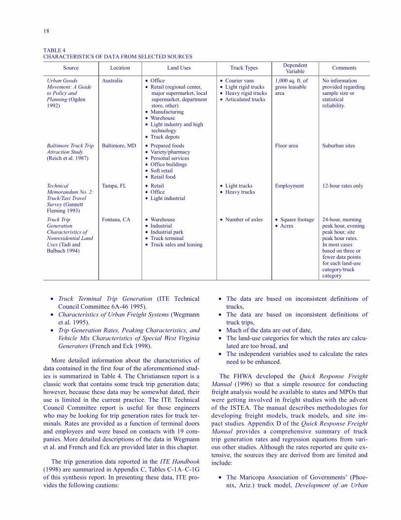
TABLE 4 CHARACTERISTICS OF DATA FROM SELECTED SOURCES

Source Location Land Uses Truck Types Dependent Variable Comments

Urban Goods Movement: A Guide to Policy and Planning (Ogden 1992)

Australia • Office • Retail (regional center,

major supermarket, local supermarket, department store, other)

• Manufacturing • Warehouse • Light industry and high

technology • Truck depots

• Courier vans • Light rigid trucks • Heavy rigid trucks • Articulated trucks

1,000 sq. ft. of gross leasable area

No information provided regarding sample size or statistical reliability.

Baltimore Truck Trip Attraction Study (Reich et al. 1987)

Baltimore, MD • Prepared foods • Variety/pharmacy • Personal services • Office buildings • Soft retail • Retail food

Floor area Suburban sites

Technical Memorandum No. 2: Truck/Taxi Travel Survey (Gannett Fleming 1993)

Tampa, FL • Retail • Office • Light industrial

• Light trucks • Heavy trucks

Employment 12-hour rates only

Truck Trip Generation Characteristics of Nonresidential Land Uses (Tadi and Balbach 1994)

Fontana, CA • Warehouse • Industrial • Industrial park • Truck terminal • Truck sales and leasing

• Number of axles • Square footage • Acres

24-hour, morning peak hour, evening peak hour, site peak hour rates. In most cases based on three or fewer data points for each land-use category/truck category

• Truck Terminal Trip Generation (ITE Technical Council Committee 6A-46 1995).

• Characteristics of Urban Freight Systems (Wegmann et al. 1995).

• Trip Generation Rates, Peaking Characteristics, and Vehicle Mix Characteristics of Special West Virginia Generators (French and Eck 1998).

More detailed information about the characteristics of data contained in the first four of the aforementioned stud-ies is summarized in Table 4. The Christiansen report is a classic work that contains some truck trip generation data; however, because these data may be somewhat dated, their use is limited in the current practice. The ITE Technical Council Committee report is useful for those engineers who may be looking for trip generation rates for truck ter-minals. Rates are provided as a function of terminal doors and employees and were based on contacts with 19 com-panies. More detailed descriptions of the data in Wegmann et al. and French and Eck are provided later in this chapter. The trip generation data reported in the ITE Handbook (1998) are summarized in Appendix C, Tables C-1A–C-1G of this synthesis report. In presenting these data, ITE pro-vides the following cautions:

• The data are based on inconsistent definitions of trucks,

• The data are based on inconsistent definitions of truck trips,

• Much of the data are out of date, • The land-use categories for which the rates are calcu-

lated are too broad, and • The independent variables used to calculate the rates

need to be enhanced. The FHWA developed the Quick Response Freight Manual (1996) so that a simple resource for conducting freight analysis would be available to states and MPOs that were getting involved in freight studies with the advent of the ISTEA. The manual describes methodologies for developing freight models, truck models, and site im-pact studies. Appendix D of the Quick Response Freight Manual provides a comprehensive summary of truck trip generation rates and regression equations from vari-ous other studies. Although the rates reported are quite ex-tensive, the sources they are derived from are limited and include:

• The Maricopa Association of Governments’ (Phoe-nix, Ariz.) truck model, Development of an Urban

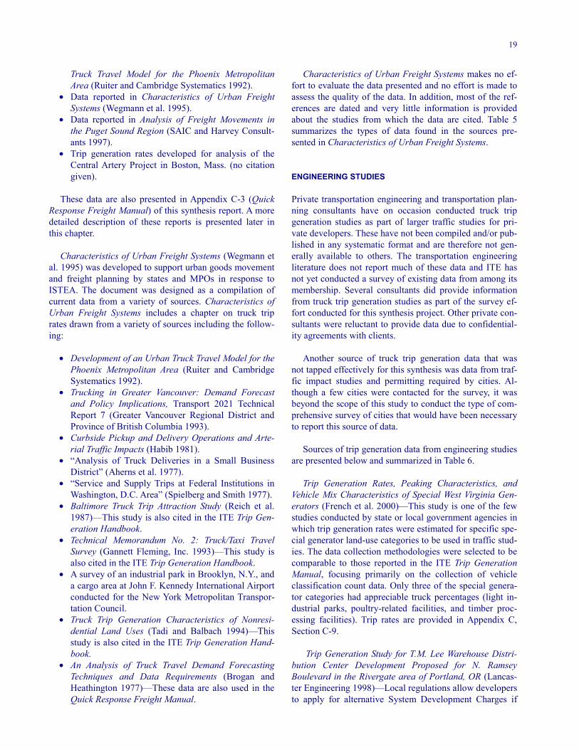
19

Truck Travel Model for the Phoenix Metropolitan Area (Ruiter and Cambridge Systematics 1992).

• Data reported in Characteristics of Urban Freight Systems (Wegmann et al. 1995).

• Data reported in Analysis of Freight Movements in the Puget Sound Region (SAIC and Harvey Consult-ants 1997).

• Trip generation rates developed for analysis of the Central Artery Project in Boston, Mass. (no citation given).

These data are also presented in Appendix C-3 (Quick Response Freight Manual) of this synthesis report. A more detailed description of these reports is presented later in this chapter. Characteristics of Urban Freight Systems (Wegmann et al. 1995) was developed to support urban goods movement and freight planning by states and MPOs in response to ISTEA. The document was designed as a compilation of current data from a variety of sources. Characteristics of Urban Freight Systems includes a chapter on truck trip rates drawn from a variety of sources including the follow-ing:

• Development of an Urban Truck Travel Model for the Phoenix Metropolitan Area (Ruiter and Cambridge Systematics 1992).

• Trucking in Greater Vancouver: Demand Forecast and Policy Implications, Transport 2021 Technical Report 7 (Greater Vancouver Regional District and Province of British Columbia 1993).

• Curbside Pickup and Delivery Operations and Arte-rial Traffic Impacts (Habib 1981).

• “Analysis of Truck Deliveries in a Small Business District” (Aherns et al. 1977).

• “Service and Supply Trips at Federal Institutions in Washington, D.C. Area” (Spielberg and Smith 1977).

• Baltimore Truck Trip Attraction Study (Reich et al. 1987)—This study is also cited in the ITE Trip Gen-eration Handbook.

• Technical Memorandum No. 2: Truck/Taxi Travel Survey (Gannett Fleming, Inc. 1993)—This study is also cited in the ITE Trip Generation Handbook.

• A survey of an industrial park in Brooklyn, N.Y., and a cargo area at John F. Kennedy International Airport conducted for the New York Metropolitan Transpor-tation Council.

• Truck Trip Generation Characteristics of Nonresi-dential Land Uses (Tadi and Balbach 1994)—This study is also cited in the ITE Trip Generation Hand-book.

• An Analysis of Truck Travel Demand Forecasting Techniques and Data Requirements (Brogan and Heathington 1977)—These data are also used in the Quick Response Freight Manual.

Characteristics of Urban Freight Systems makes no ef-fort to evaluate the data presented and no effort is made to assess the quality of the data. In addition, most of the ref-erences are dated and very little information is provided about the studies from which the data are cited. Table 5 summarizes the types of data found in the sources pre-sented in Characteristics of Urban Freight Systems. ENGINEERING STUDIES Private transportation engineering and transportation plan-ning consultants have on occasion conducted truck trip generation studies as part of larger traffic studies for pri-vate developers. These have not been compiled and/or pub-lished in any systematic format and are therefore not gen-erally available to others. The transportation engineering literature does not report much of these data and ITE has not yet conducted a survey of existing data from among its membership. Several consultants did provide information from truck trip generation studies as part of the survey ef-fort conducted for this synthesis project. Other private con-sultants were reluctant to provide data due to confidential-ity agreements with clients. Another source of truck trip generation data that was not tapped effectively for this synthesis was data from traf-fic impact studies and permitting required by cities. Al-though a few cities were contacted for the survey, it was beyond the scope of this study to conduct the type of com-prehensive survey of cities that would have been necessary to report this source of data. Sources of trip generation data from engineering studies are presented below and summarized in Table 6. Trip Generation Rates, Peaking Characteristics, and Vehicle Mix Characteristics of Special West Virginia Gen-erators (French et al. 2000)—This study is one of the few studies conducted by state or local government agencies in which trip generation rates were estimated for specific spe-cial generator land-use categories to be used in traffic stud-ies. The data collection methodologies were selected to be comparable to those reported in the ITE Trip Generation Manual, focusing primarily on the collection of vehicle classification count data. Only three of the special genera-tor categories had appreciable truck percentages (light in-dustrial parks, poultry-related facilities, and timber proc-essing facilities). Trip rates are provided in Appendix C, Section C-9. Trip Generation Study for T.M. Lee Warehouse Distri-bution Center Development Proposed for N. Ramsey Boulevard in the Rivergate area of Portland, OR (Lancas-ter Engineering 1998)—Local regulations allow developers to apply for alternative System Development Charges if

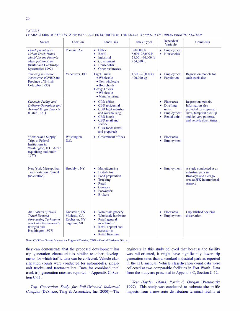
20

TABLE 5 CHARACTERISTICS OF DATA FROM SELECTED SOURCES IN THE CHARACTERISTICS OF URBAN FREIGHT SYSTEMS

Source Location Land Uses Truck Types Dependent Variable

Comments Development of an Urban Truck Travel Model for the Phoenix Metropolitan Area (Ruiter and Cambridge Systematics 1992)

Phoenix, AZ • Office • Retail • Industrial • Government • Households • Other businesses

0–8,000 lb 8,001–28,000 lb 28,001–64,000 lb >64,000 lb

• Employment • Households

Trucking in Greater Vancouver (GVRD and Province of British Columbia 1993)

Vancouver, BC Light Trucks • Wholesale • Non-wholesale • Households

Heavy Trucks • Wholesale • Manufacturing

4,500–20,000 kg >20,000 kg

• Employment • Population

Regression models for each truck size

Curbside Pickup and Delivery Operations and Arterial Traffic Impacts (Habib 1981)

• CBD office • CBD residential • CBD light industry

and warehousing • CBD hotels • CBD retail and

service • CBD foods (retail

and prepared)

• Floor area • Dwelling

units • Employment • Rental units

Regression models. Information also provided for shipment sizes, temporal pick-up and delivery patterns, and vehicle dwell times.

“Service and Supply Trips at Federal Institutions in Washington, D.C. Area” (Spielberg and Smith 1977)

Washington, D.C.

• Government offices

• Floor area • Employment

New York Metropolitan Transportation Council (no citation)

Brooklyn, NY • Manufacturing • Distribution • Food preparation • Trucking • Retail • Couriers • Forwarders • Brokers

• Employment A study conducted at an industrial park in Brooklyn and a cargo area at JFK International Airport.

An Analysis of Truck Travel Demand Forecasting Techniques and Data Requirements (Brogan and Heathington 1977)

Knoxville, TN Modesto, CA Rochester, NY Saginaw, MI

• Wholesale grocery • Wholesale hardware • Retail general

merchandise • Retail apparel and

accessories • Retail furniture

• Floor area • Employment

Unpublished doctoral dissertation

Note: GVRD = Greater Vancouver Regional District; CBD = Central Business District. they can demonstrate that the proposed development has trip generation characteristics similar to other develop-ments for which traffic data can be collected. Vehicle clas-sification counts were conducted for automobiles, single-unit trucks, and tractor-trailers. Data for combined total truck trip generation rates are reported in Appendix C, Sec-tion C-11. Trip Generation Study for Rail-Oriented Industrial Complex (DeShazo, Tang & Associates, Inc. 2000)—The

engineers in this study believed that because the facility was rail-oriented, it might have significantly lower trip generation rates than a standard industrial park as reported in the ITE manual. Vehicle classification count data were collected at two comparable facilities in Fort Worth. Data from the study are presented in Appendix C, Section C-12. West Hayden Island, Portland, Oregon (Parametrix 1999)—This study was conducted to estimate site traffic impacts from a new auto distribution terminal facility at

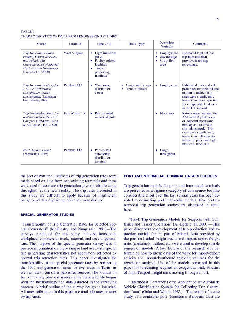
21

TABLE 6 CHARACTERISTICS OF DATA FROM ENGINEERING STUDIES

Source Location Land Uses Truck Types Dependent Variable

Comments

Trip Generation Rates, Peaking Characteristics, and Vehicle Mix Characteristics of Special West Virginia Generators (French et al. 2000)

West Virginia • Light industrial parks

• Poultry-related facilities

• Timber processing facilities

• Employment • Site acreage • Gross floor

area

Estimated total vehicle trip rates and then provided truck trip percentage.

Trip Generation Study for T.M. Lee Warehouse Distribution Center Development (Lancaster Engineering 1998)

Portland, OR • Warehouse distribution center

• Single-unit trucks • Tractor-trailers

• Employment

Calculated peak and off-peak rates for inbound and outbound traffic. Trip rates were significantly lower than those reported for comparable land uses in the ITE manual.

Trip Generation Study for Rail-Oriented Industrial Complex (DeShazo, Tang & Associates, Inc. 2000)

Fort Worth, TX • Rail-oriented industrial park

• Floor area

Rates were calculated for AM and PM peak hours on adjacent streets and midday and afternoon site-related peak. Trip rates were significantly lower than ITE rates for industrial parks and light industrial land uses

West Hayden Island (Parametrix 1999)

Portland, OR • Port-related automobile distribution terminal

• Cargo throughput

the port of Portland. Estimates of trip generation rates were made based on data from two existing terminals and these were used to estimate trip generation given probable cargo throughput at the new facility. The trip rates presented in this study are difficult to apply because of insufficient background data explaining how they were derived. SPECIAL GENERATOR STUDIES “Transferability of Trip Generation Rates for Selected Spe-cial Generators” (McKinstry and Nungesser 1991)—The surveys conducted for this study included household, workplace, commercial truck, external, and special genera-tors. The purpose of the special generator survey was to provide information on those unique land uses with special trip generating characteristics not adequately reflected by normal trip attraction rates. This paper investigates the transferability of the special generator rates by comparing the 1990 trip generation rates for two areas in Texas, as well as rates from other published sources. The foundation for comparing rates and assessing the transferability begins with the methodology and data gathered in the surveying process. A brief outline of the survey design is included. All rates referred to in this paper are total trip rates or rates by trip ends.

PORT AND INTERMODAL TERMINAL DATA RESOURCES Trip generation models for ports and intermodal terminals are presented as a separate category of data source because considerable effort over the last several years has been de-voted to estimating port/intermodal models. Five port/in-termodal trip generation studies are discussed in detail here. “Truck Trip Generation Models for Seaports with Con-tainer and Trailer Operation” (Al-Deek et al. 2000)—This paper describes the development of trip production and at-traction models for the port of Miami. Data provided by the port on loaded freight trucks and import/export freight units (containers, trailers, etc.) were used to develop simple regression models. A key feature of the research was de-termining how to group days of the week for import/export activity and inbound/outbound trucking volumes for the regression analysis. Use of the models contained in this paper for forecasting requires an exogenous trade forecast of import/export freight units moving through a port. “Intermodal Container Ports: Application of Automatic Vehicle Classification System for Collecting Trip Genera-tion Data” (Guha and Walton 1983)—The results of a case study of a container port (Houston’s Barbours Cut) are

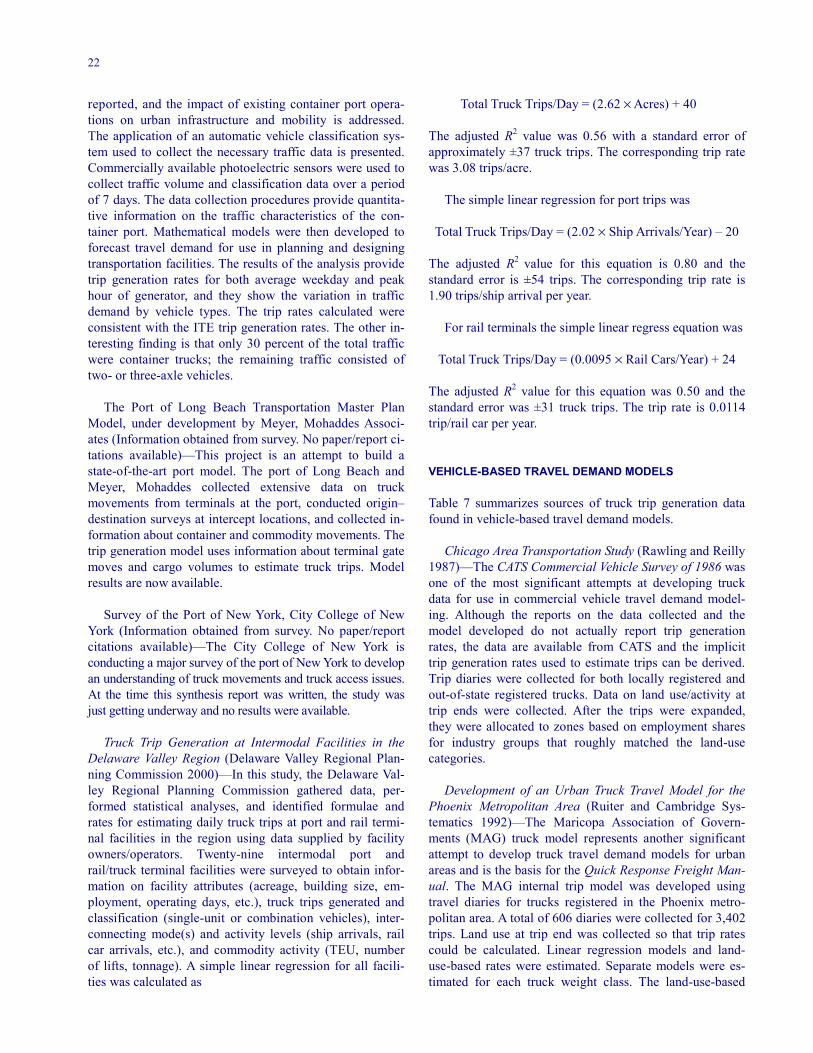
22

reported, and the impact of existing container port opera-tions on urban infrastructure and mobility is addressed. The application of an automatic vehicle classification sys-tem used to collect the necessary traffic data is presented. Commercially available photoelectric sensors were used to collect traffic volume and classification data over a period of 7 days. The data collection procedures provide quantita-tive information on the traffic characteristics of the con-tainer port. Mathematical models were then developed to forecast travel demand for use in planning and designing transportation facilities. The results of the analysis provide trip generation rates for both average weekday and peak hour of generator, and they show the variation in traffic demand by vehicle types. The trip rates calculated were consistent with the ITE trip generation rates. The other in-teresting finding is that only 30 percent of the total traffic were container trucks; the remaining traffic consisted of two- or three-axle vehicles. The Port of Long Beach Transportation Master Plan Model, under development by Meyer, Mohaddes Associ-ates (Information obtained from survey. No paper/report ci-tations available)—This project is an attempt to build a state-of-the-art port model. The port of Long Beach and Meyer, Mohaddes collected extensive data on truck movements from terminals at the port, conducted origin–destination surveys at intercept locations, and collected in-formation about container and commodity movements. The trip generation model uses information about terminal gate moves and cargo volumes to estimate truck trips. Model results are now available. Survey of the Port of New York, City College of New York (Information obtained from survey. No paper/report citations available)—The City College of New York is conducting a major survey of the port of New York to develop an understanding of truck movements and truck access issues. At the time this synthesis report was written, the study was just getting underway and no results were available. Truck Trip Generation at Intermodal Facilities in the Delaware Valley Region (Delaware Valley Regional Plan-ning Commission 2000)—In this study, the Delaware Val-ley Regional Planning Commission gathered data, per-formed statistical analyses, and identified formulae and rates for estimating daily truck trips at port and rail termi-nal facilities in the region using data supplied by facility owners/operators. Twenty-nine intermodal port and rail/truck terminal facilities were surveyed to obtain infor-mation on facility attributes (acreage, building size, em-ployment, operating days, etc.), truck trips generated and classification (single-unit or combination vehicles), inter-connecting mode(s) and activity levels (ship arrivals, rail car arrivals, etc.), and commodity activity (TEU, number of lifts, tonnage). A simple linear regression for all facili-ties was calculated as

Total Truck Trips/Day = (2.62 × Acres) + 40 The adjusted R2 value was 0.56 with a standard error of approximately ±37 truck trips. The corresponding trip rate was 3.08 trips/acre. The simple linear regression for port trips was Total Truck Trips/Day = (2.02 × Ship Arrivals/Year) – 20

The adjusted R2 value for this equation is 0.80 and the standard error is ±54 trips. The corresponding trip rate is 1.90 trips/ship arrival per year. For rail terminals the simple linear regress equation was

Total Truck Trips/Day = (0.0095 × Rail Cars/Year) + 24 The adjusted R2 value for this equation was 0.50 and the standard error was ±31 truck trips. The trip rate is 0.0114 trip/rail car per year. VEHICLE-BASED TRAVEL DEMAND MODELS Table 7 summarizes sources of truck trip generation data found in vehicle-based travel demand models. Chicago Area Transportation Study (Rawling and Reilly 1987)—The CATS Commercial Vehicle Survey of 1986 was one of the most significant attempts at developing truck data for use in commercial vehicle travel demand model-ing. Although the reports on the data collected and the model developed do not actually report trip generation rates, the data are available from CATS and the implicit trip generation rates used to estimate trips can be derived. Trip diaries were collected for both locally registered and out-of-state registered trucks. Data on land use/activity at trip ends were collected. After the trips were expanded, they were allocated to zones based on employment shares for industry groups that roughly matched the land-use categories. Development of an Urban Truck Travel Model for the Phoenix Metropolitan Area (Ruiter and Cambridge Sys-tematics 1992)—The Maricopa Association of Govern-ments (MAG) truck model represents another significant attempt to develop truck travel demand models for urban areas and is the basis for the Quick Response Freight Man-ual. The MAG internal trip model was developed using travel diaries for trucks registered in the Phoenix metro-politan area. A total of 606 diaries were collected for 3,402 trips. Land use at trip end was collected so that trip rates could be calculated. Linear regression models and land-use-based rates were estimated. Separate models were es-timated for each truck weight class. The land-use-based

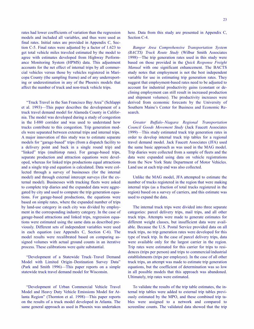
23

rates had lower coefficients of variation than the regression models and included all variables, and thus were used as final rates. Initial rates are provided in Appendix C, Sec-tion C-5. Final rates were adjusted by a factor of 1.623 to get total vehicle miles traveled estimated by the model to agree with estimates developed from Highway Perform-ance Monitoring System (HPMS) data. This adjustment accounts for the net effect of internal trips by all commer-cial vehicles versus those by vehicles registered in Mari-copa County (the sampling frame) and of any underreport-ing or underestimation in any of the Phoenix models that affect the number of truck and non-truck vehicle trips. “Truck Travel in the San Francisco Bay Area” (Schlappi et al. 1993)—This paper describes the development of a truck travel demand model for Alameda County in Califor-nia. The model was developed during a study of congestion in the I-880 corridor and was used to understand how trucks contribute to this congestion. Trip generation mod-els were separated between external trips and internal trips. A major innovation of this study was to estimate separate models for “garage-based” trips (from a dispatch facility to a delivery point and back in a single round trip) and “linked” trips (multistop runs). For garage-based trips, separate production and attraction equations were devel-oped, whereas for linked trips productions equal attractions and a single trip end equation is calculated. Data were col-lected through a survey of businesses (for the internal model) and through external intercept surveys (for the ex-ternal model). Businesses with trucking fleets were asked to complete trip diaries and the expanded data were aggre-gated by city and used to compute the trip generation equa-tions. For garage-based productions, the equations were based on simple rates, where the expanded number of trips by land-use category in each city was divided by employ-ment in the corresponding industry category. In the case of garage-based attractions and linked trips, regression equa-tions were estimated using the same data as described pre-viously. Different sets of independent variables were used in each equation (see Appendix C, Section C-6). The model results were recalibrated based on comparing as-signed volumes with actual ground counts in an iterative process. These calibrations were quite substantial. “Development of a Statewide Truck–Travel Demand Model with Limited Origin–Destination Survey Data” (Park and Smith 1996)—This paper reports on a simple statewide truck travel demand model for Wisconsin. “Development of Urban Commercial Vehicle Travel Model and Heavy Duty Vehicle Emissions Model for At-lanta Region” (Thornton et al. 1998)—This paper reports on the results of a truck model developed in Atlanta. The same general approach as used in Phoenix was undertaken

here. Data from this study are presented in Appendix C, Section C-4. Bangor Area Comprehensive Transportation System (BACTS) Truck Route Study (Wilbur Smith Associates 1998)—The trip generation rates used in this study were based on those provided in the Quick Response Freight Manual with one significant enhancement. The BACTS study notes that employment is not the best independent variable for use in estimating trip generation rates. They suggest that employment-based rates need to be adjusted to account for industrial productivity gains (constant or de-clining employment can still result in increased production and shipment volumes). The productivity increases were derived from economic forecasts by the University of Southern Maine’s Center for Business and Economic Re-search. Greater Buffalo–Niagara Regional Transportation Council Goods Movement Study (Jack Faucett Associates 1999)—This study estimated truck trip generation rates in order to develop internal truck trip tables for a regional travel demand model. Jack Faucett Associates (JFA) used the same basic approach as was used in the MAG model. Trip diaries were collected from a sample of fleets and the data were expanded using data on vehicle registrations from the New York State Department of Motor Vehicles. Land use at each trip end was also collected. Unlike the MAG model, JFA attempted to estimate the number of trucks registered in the region that were making internal trips (as a fraction of total trucks registered in the region) based on a survey of carriers, and this estimate was used to expand the data. The internal truck trips were divided into three separate categories: parcel delivery trips, mail trips, and all other truck trips. Attempts were made to generate estimates for different weight classes, but insufficient data were avail-able. Because the U.S. Postal Service provided data on all truck trips, no trip generation rates were developed for this type of truck trip. In the case of parcel delivery trips, data were available only for the largest carrier in the region. Trip rates were estimated for this carrier for trips to resi-dences (trips per person) and trips to commercial/industrial establishments (trips per employee). In the case of all other truck trips, an attempt was made to estimate trip generation equations, but the coefficient of determination was so low in all possible models that this approach was abandoned. Ultimately, trip rates were estimated. To validate the results of the trip table estimates, the in-ternal trip tables were added to external trip tables previ-ously estimated by the MPO, and these combined trip ta-bles were assigned to a network and compared to screenline counts. The validated data showed that the trip

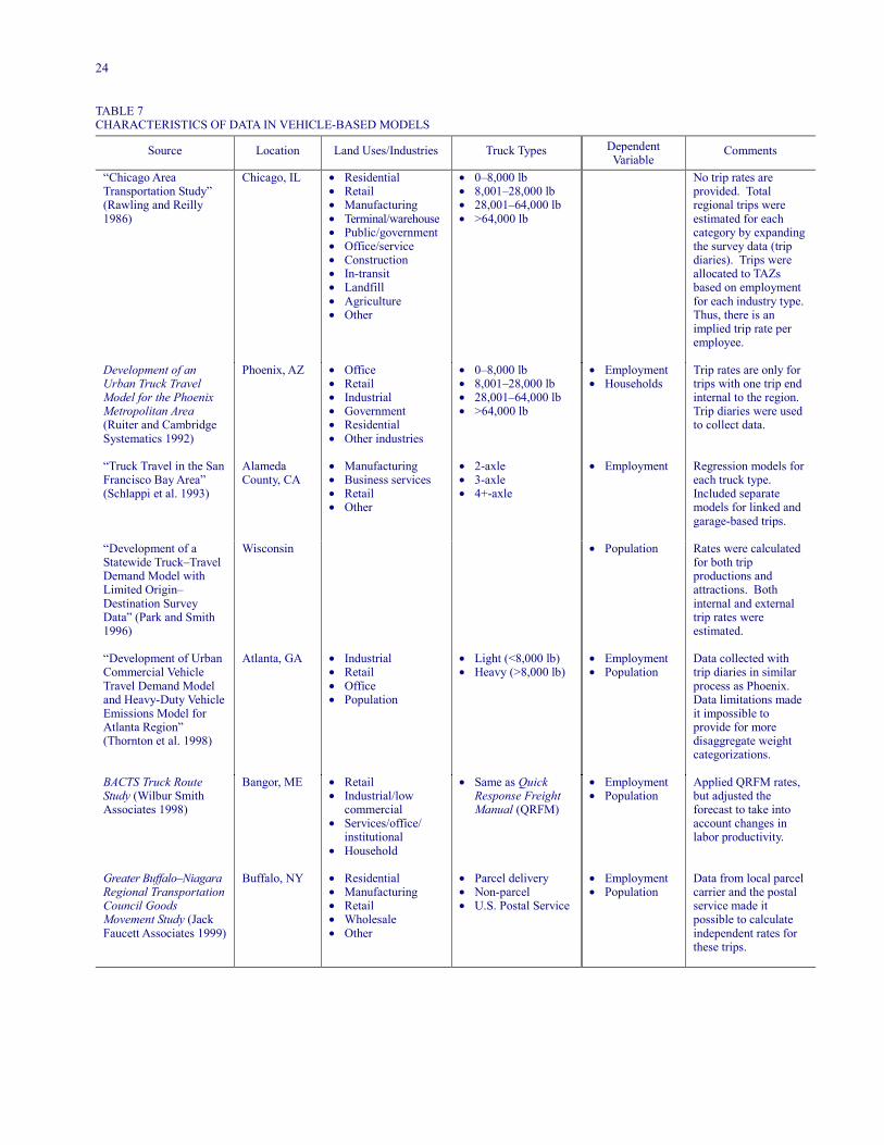
24

TABLE 7 CHARACTERISTICS OF DATA IN VEHICLE-BASED MODELS

Source Location Land Uses/Industries Truck Types Dependent Variable

Comments

“Chicago Area Transportation Study” (Rawling and Reilly 1986)

Chicago, IL • Residential • Retail • Manufacturing • Terminal/warehouse • Public/government • Office/service • Construction • In-transit • Landfill • Agriculture • Other

• 0–8,000 lb • 8,001–28,000 lb • 28,001–64,000 lb • >64,000 lb

No trip rates are provided. Total regional trips were estimated for each category by expanding the survey data (trip diaries). Trips were allocated to TAZs based on employment for each industry type. Thus, there is an implied trip rate per employee.

Development of an Urban Truck Travel Model for the Phoenix Metropolitan Area (Ruiter and Cambridge Systematics 1992)

Phoenix, AZ • Office • Retail • Industrial • Government • Residential • Other industries

• 0–8,000 lb • 8,001–28,000 lb • 28,001–64,000 lb • >64,000 lb

• Employment • Households

Trip rates are only for trips with one trip end internal to the region. Trip diaries were used to collect data.

“Truck Travel in the San Francisco Bay Area” (Schlappi et al. 1993)

Alameda County, CA

• Manufacturing • Business services • Retail • Other

• 2-axle • 3-axle • 4+-axle

• Employment

Regression models for each truck type. Included separate models for linked and garage-based trips.

“Development of a Statewide Truck–Travel Demand Model with Limited Origin–Destination Survey Data” (Park and Smith 1996)

Wisconsin • Population Rates were calculated for both trip productions and attractions. Both internal and external trip rates were estimated.

“Development of Urban Commercial Vehicle Travel Demand Model and Heavy-Duty Vehicle Emissions Model for Atlanta Region” (Thornton et al. 1998)

Atlanta, GA • Industrial • Retail • Office • Population

• Light (<8,000 lb) • Heavy (>8,000 lb)

• Employment • Population

Data collected with trip diaries in similar process as Phoenix. Data limitations made it impossible to provide for more disaggregate weight categorizations.

BACTS Truck Route Study (Wilbur Smith Associates 1998)

Bangor, ME • Retail • Industrial/low

commercial • Services/office/ institutional • Household

• Same as Quick Response Freight Manual (QRFM)

• Employment • Population

Applied QRFM rates, but adjusted the forecast to take into account changes in labor productivity.

Greater Buffalo–Niagara Regional Transportation Council Goods Movement Study (Jack Faucett Associates 1999)

Buffalo, NY • Residential • Manufacturing • Retail • Wholesale • Other

• Parcel delivery • Non-parcel • U.S. Postal Service

• Employment • Population

Data from local parcel carrier and the postal service made it possible to calculate independent rates for these trips.

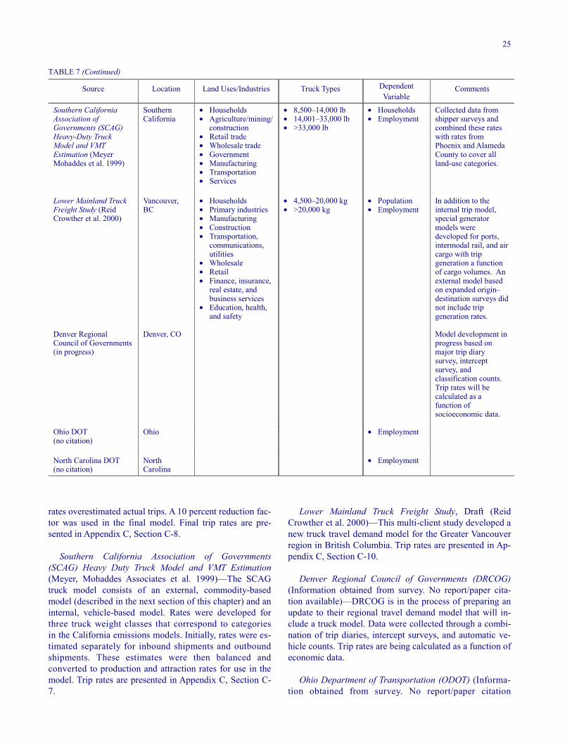
25

TABLE 7 (Continued) Source Location Land Uses/Industries Truck Types Dependent

Variable Comments

Southern California Association of Governments (SCAG) Heavy-Duty Truck Model and VMT Estimation (Meyer Mohaddes et al. 1999)

Southern California

• Households • Agriculture/mining/ construction • Retail trade • Wholesale trade • Government • Manufacturing • Transportation • Services

• 8,500–14,000 lb • 14,001–33,000 lb • >33,000 lb

• Households • Employment

Collected data from shipper surveys and combined these rates with rates from Phoenix and Alameda County to cover all land-use categories.

Lower Mainland Truck Freight Study (Reid Crowther et al. 2000)

Vancouver, BC

• Households • Primary industries • Manufacturing • Construction • Transportation,

communications, utilities

• Wholesale • Retail • Finance, insurance,

real estate, and business services

• Education, health, and safety

• 4,500–20,000 kg • >20,000 kg

• Population • Employment

In addition to the internal trip model, special generator models were developed for ports, intermodal rail, and air cargo with trip generation a function of cargo volumes. An external model based on expanded origin–destination surveys did not include trip generation rates.

Denver Regional Council of Governments (in progress)

Denver, CO Model development in progress based on major trip diary survey, intercept survey, and classification counts. Trip rates will be calculated as a function of socioeconomic data.

Ohio DOT (no citation)

Ohio • Employment

North Carolina DOT (no citation)

North Carolina

• Employment

rates overestimated actual trips. A 10 percent reduction fac-tor was used in the final model. Final trip rates are pre-sented in Appendix C, Section C-8. Southern California Association of Governments (SCAG) Heavy Duty Truck Model and VMT Estimation (Meyer, Mohaddes Associates et al. 1999)—The SCAG truck model consists of an external, commodity-based model (described in the next section of this chapter) and an internal, vehicle-based model. Rates were developed for three truck weight classes that correspond to categories in the California emissions models. Initially, rates were es-timated separately for inbound shipments and outbound shipments. These estimates were then balanced and converted to production and attraction rates for use in the model. Trip rates are presented in Appendix C, Section C-7.

Lower Mainland Truck Freight Study, Draft (Reid Crowther et al. 2000)—This multi-client study developed a new truck travel demand model for the Greater Vancouver region in British Columbia. Trip rates are presented in Ap-pendix C, Section C-10. Denver Regional Council of Governments (DRCOG) (Information obtained from survey. No report/paper cita-tion available)—DRCOG is in the process of preparing an update to their regional travel demand model that will in-clude a truck model. Data were collected through a combi-nation of trip diaries, intercept surveys, and automatic ve-hicle counts. Trip rates are being calculated as a function of economic data. Ohio Department of Transportation (ODOT) (Informa-tion obtained from survey. No report/paper citation

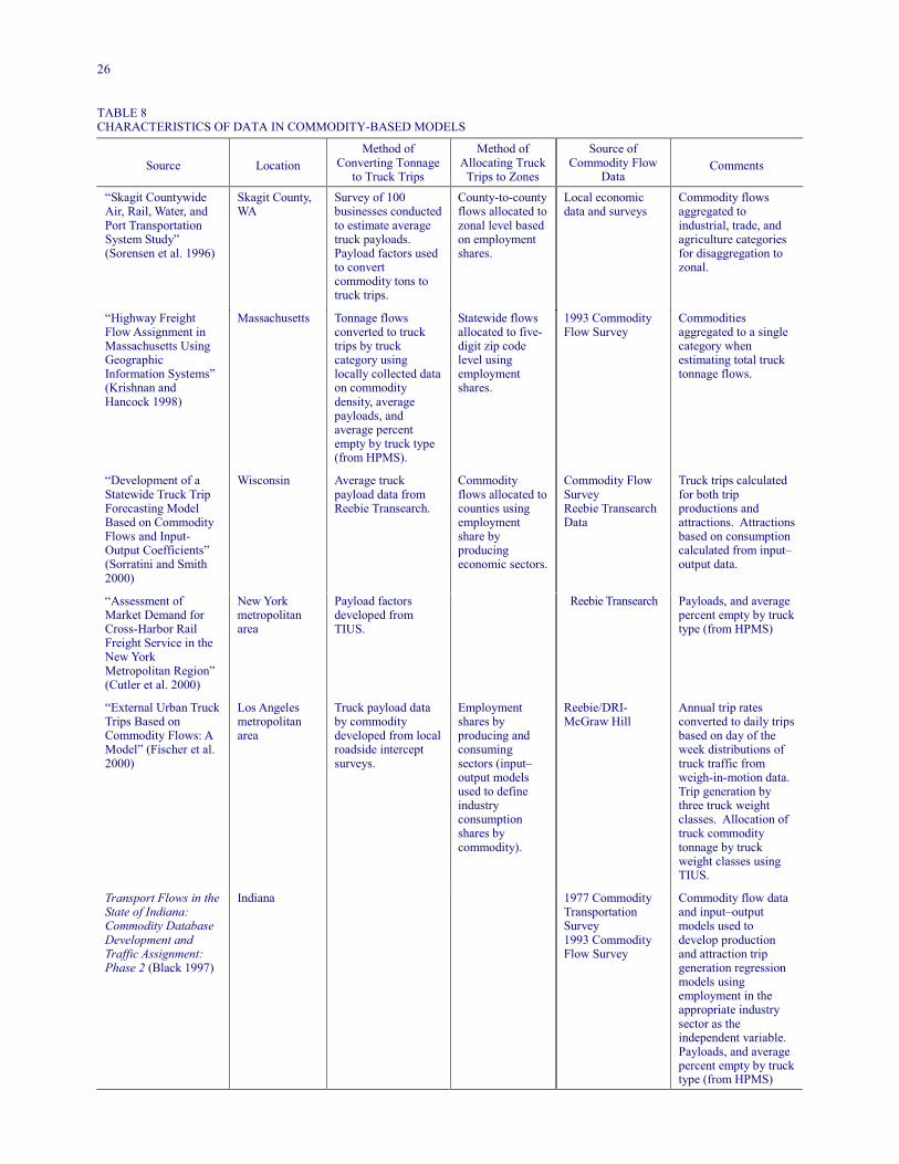
26

TABLE 8 CHARACTERISTICS OF DATA IN COMMODITY-BASED MODELS

Source

Location

Method of Converting Tonnage

to Truck Trips

Method of Allocating Truck

Trips to Zones

Source of Commodity Flow

Data

Comments

“Skagit Countywide Air, Rail, Water, and Port Transportation System Study” (Sorensen et al. 1996)

Skagit County, WA

Survey of 100 businesses conducted to estimate average truck payloads. Payload factors used to convert commodity tons to truck trips.

County-to-county flows allocated to zonal level based on employment shares.

Local economic data and surveys

Commodity flows aggregated to industrial, trade, and agriculture categories for disaggregation to zonal.

“Highway Freight Flow Assignment in Massachusetts Using Geographic Information Systems” (Krishnan and Hancock 1998)

Massachusetts Tonnage flows converted to truck trips by truck category using locally collected data on commodity density, average payloads, and average percent empty by truck type (from HPMS).

Statewide flows allocated to five-digit zip code level using employment shares.

1993 Commodity Flow Survey

Commodities aggregated to a single category when estimating total truck tonnage flows.

“Development of a Statewide Truck Trip Forecasting Model Based on Commodity Flows and Input-Output Coefficients” (Sorratini and Smith 2000)

Wisconsin Average truck payload data from Reebie Transearch.

Commodity flows allocated to counties using employment share by producing economic sectors.

Commodity Flow Survey Reebie Transearch Data

Truck trips calculated for both trip productions and attractions. Attractions based on consumption calculated from input–output data.

“Assessment of Market Demand for Cross-Harbor Rail Freight Service in the New York Metropolitan Region” (Cutler et al. 2000)

New York metropolitan area

Payload factors developed from TIUS.

Reebie Transearch Payloads, and average percent empty by truck type (from HPMS)

“External Urban Truck Trips Based on Commodity Flows: A Model” (Fischer et al. 2000)

Los Angeles metropolitan area

Truck payload data by commodity developed from local roadside intercept surveys.

Employment shares by producing and consuming sectors (input–output models used to define industry consumption shares by commodity).

Reebie/DRI-McGraw Hill

Annual trip rates converted to daily trips based on day of the week distributions of truck traffic from weigh-in-motion data. Trip generation by three truck weight classes. Allocation of truck commodity tonnage by truck weight classes using TIUS.

Transport Flows in the State of Indiana: Commodity Database Development and Traffic Assignment: Phase 2 (Black 1997)

Indiana 1977 Commodity Transportation Survey 1993 Commodity Flow Survey

Commodity flow data and input–output models used to develop production and attraction trip generation regression models using employment in the appropriate industry sector as the independent variable. Payloads, and average percent empty by truck type (from HPMS)

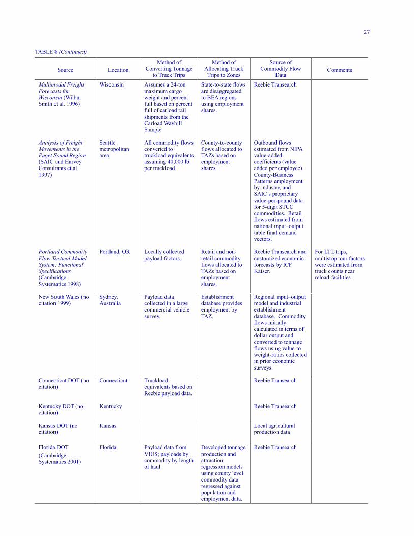
27

TABLE 8 (Continued)

Source

Location Method of

Converting Tonnage to Truck Trips

Method of Allocating Truck

Trips to Zones

Source of Commodity Flow

Data

Comments

Multimodal Freight Forecasts for Wisconsin (Wilbur Smith et al. 1996)

Wisconsin Assumes a 24-ton maximum cargo weight and percent full based on percent full of carload rail shipments from the Carload Waybill Sample.

State-to-state flows are disaggregated to BEA regions using employment shares.

Reebie Transearch

Analysis of Freight Movements in the Puget Sound Region (SAIC and Harvey Consultants et al. 1997)

Seattle metropolitan area

All commodity flows converted to truckload equivalents assuming 40,000 lb per truckload.

County-to-county flows allocated to TAZs based on employment shares.

Outbound flows estimated from NIPA value-added coefficients (value added per employee), County-Business Patterns employment by industry, and SAIC’s proprietary value-per-pound data for 5-digit STCC commodities. Retail flows estimated from national input–output table final demand vectors.

Portland Commodity Flow Tactical Model System: Functional Specifications (Cambridge Systematics 1998)

Portland, OR Locally collected payload factors.

Retail and non-retail commodity flows allocated to TAZs based on employment shares.

Reebie Transearch and customized economic forecasts by ICF Kaiser.

For LTL trips, multistop tour factors were estimated from truck counts near reload facilities.

New South Wales (no citation 1999)

Sydney, Australia

Payload data collected in a large commercial vehicle survey.

Establishment database provides employment by TAZ.

Regional input–output model and industrial establishment database. Commodity flows initially calculated in terms of dollar output and converted to tonnage flows using value-to weight-ratios collected in prior economic surveys.

Connecticut DOT (no citation)

Connecticut Truckload equivalents based on Reebie payload data.

Reebie Transearch

Kentucky DOT (no citation)

Kentucky Reebie Transearch

Kansas DOT (no citation)

Kansas Local agricultural production data

Florida DOT (Cambridge Systematics 2001)

Florida Payload data from VIUS; payloads by commodity by length of haul.

Developed tonnage production and attraction regression models using county level commodity data regressed against population and employment data.

Reebie Transearch

28

available)—ODOT reports having developed truck trip generation data for both statewide and regional travel de-mand modeling. The data were collected primarily from in-tercept surveys. Trip generation equations were estimated with regression equations. North Carolina Department of Transportation (Informa-tion obtained from survey. No report/paper citation avail-able)—Barton Aschman developed truck trip generation data for regional models in North Carolina. The rates were developed primarily from trip diary surveys. Separate pro-duction and attraction rates were estimated by land-use/industry type. COMMODITY-BASED TRAVEL DEMAND MODELS Table 8 summarizes sources of truck trip generation data found in commodity-based models. “Skagit Countywide Air, Rail, Water, and Port Transpor-tation System Study” (Sorensen et al. 1996)—This paper reports on a commodity flow study of Skagit County, Washington, and presents a methodology for estimating truck flows based on commodity data. This is one of the few commodity-based trip generation studies that provides sufficient socioeconomic data for the computation of equivalent trip rates per 1,000 employees. These data are presented in Appendix C, Section C-2. “Highway Freight Flow Assignment in Massachusetts Using Geographic Information Systems” (Krishnan and Hancock 1998)—This paper presents an approach to mod-eling statewide truck flows based on commodity flow data. Trip generation data are developed at the five-digit zip code level for the state of Massachusetts. The general pro-cedures used for trip generation in this study are similar to those used in other studies based on commodity flows, al-though the specific commodity flow data and truck pay-load data are somewhat unique. “Development of a Statewide Truck Trip Forecasting Model Based on Commodity Flows and Input-Output Co-efficients” (Sorratini and Smith 2000)—This work builds on that of Park and Smith by creating a more complete commodity-based statewide truck trip model for Wiscon-sin. The model estimates trip productions and attractions from a combination of commodity flow data and economic input–output models. Consumption by economic sector was estimated using economic input–output models. “Assessment of Market Demand for Cross-Harbor Rail Freight Service in the New York Metropolitan Region” (Cutler et al. 2000)—This paper describes an analysis of potential diversion of cross-harbor truck traffic to rail in the event that a new harbor rail freight tunnel is provided.

Like most of the other commodity-based methodologies, the basic approach to trip generation was to use tonnage flows by commodity group and to translate these to truck trips using truck payload factors by commodity group. “External Urban Truck Trips Based on Commodity Flows: A Model” (Fischer et al. 2000)—This paper de-scribes the approach to modeling external truck trips in the recently developed regional heavy-duty truck travel de-mand model of SCAG. The SCAG truck model includes an internal trip generation and distribution model that uses procedures more akin to 4-step urban travel demand mod-els (the trip generation data from this element of the model are described earlier in this chapter) while the external model is based on a commodity flow model. Two-digit Standard Transportation Commodity Classification (STCC) categories were used in the development of the model. Transport Flows in the State of Indiana: Commodity Database Development and Traffic Assignment: Phase 2 (Black 1997)—This is a statewide truck trip model that was originally developed for the Indiana DOT by Indiana University (Black 1997) and later incorporated by Cam-bridge Systematics in the Indiana Statewide Travel De-mand Model. This is a commodity-based model that cate-gorizes truck trips on the basis of payloads, and average percent empty by truck type (from HPMS) of 19 different commodity groups (based on the STCC system), mail (data from the postal service), and express mail (based on data from Federal Express). The initial trip generation equations are not mode specific. A set of mode split equations was developed based on the mode split for Indiana in the 1993 CFS. The mode shares were developed for different com-modities and lengths of haul. Multimodal Freight Forecasts for Wisconsin (Wilbur Smith Associates and Reebie Associates 1996)—This study, prepared by Wilbur Smith Associates in association with Reebie Associates, represents the culmination of a number of studies aimed at developing a statewide freight model based on commodity flow data and input–output economic modeling techniques. The study only looks at intercity truck trips. The starting point for the analysis was Reebie Transearch data. The approach to developing these data is to start with Census of Manufacturers value of shipment data. This is converted to tonnage based on value-to-weight ratios in Reebie’s proprietary database and allocated to states of origin based on employment shares in producing industries. Modal share is determined by sub-tracting known modal tonnage from federal data sources. The residual is assumed to be truck. State-to-state flows are estimated using data obtained by Reebie from trucking firms in a data exchange program, as are the distribution of flows by sub-mode (e.g., truckload, less-than-truckload, and private trucking fleets). The commodity flows are further disaggregated to Business Economic Areas [multi-county

29

aggregates developed by the U.S. Bureau of Economic Analysis (BEA)] using employment shares and the in-bound commodity flows are developed using input–output coefficients. Secondary movements (distribution traffic primarily from wholesalers to retailers) are estimated based on information from the Reebie data exchange program. Nonmanufactured goods are added using production and consumption data developed locally. Conversion to truck-loads was accomplished using a 24-ton maximum cargo weight for each truck and using the percentage of full car-load ratios for each commodity from the Interstate Com-merce Commission’s (now Surface Transportation Board) Carload Waybill Sample data applied to truckloads. The Waybill sample provides data on a sample of rail moves in the United States. These data include the carload weights. By comparing average carload weights for each commod-ity group as compared to maximum carload weight a ratio was calculated and this ratio was applied to truck data to estimate payloads for each commodity when carried by a truck. Annual truckload equivalents were divided by 310 operating days to get daily truck trips. These were disag-gregated to the county level based on employment shares. Empties were also added. Because there is no direct calculation of trip generation rates, the methodology is perhaps the most useful piece of this study (see Fig. 3). Analysis of Freight Movements in the Puget Sound Re-gion (SAIC and Harvey Consultants 1997)—The truck trip generation rates developed in this study are reported in truckload equivalents (TLEs), although there appears to be some effort to convert these to actual truck trips. After calibration to truck counts, the resulting trip generation rates have been used for corridor studies in the Puget Sound Region. Four categories of truck trips are identified for estimating truck trip generation rates.

Long haul—Trips into and out of an area with desti-nations more than 250 miles away from the origin. These truck trips are made primarily by for-hire mo-tor carriers. Most of the outbound trips come from the manufacturing sector.

Short haul—These trips move within approximately a 250-mile radius of the origin. A major source of these trips is wholesale to retail movements. They also include many trip chains returning to home base empty at the end of the day. This category also in-cludes raw materials moving in local markets. Carri-ers are often private fleets with drivers domiciled at home or regional less-than-truckload/specialty carri-ers. The category also includes some movements of manufacturing inputs through wholesalers.

Local Traffic—Such trips are primarily local delivery operations and are small shipments. This category in-

cludes some wholesale to retail movements and wholesale to local manufacturer movements. These are primarily linked trips and account for the pre-ponderance of trips in a local area. It also includes service vehicles. In addition, this category includes the movement by truck from one mode to another (drayage). Through Traffic—Trips with both origin and destina-tion outside the Puget Sound region.

To develop manufacturing truck flows, the consultant used industry-sector National Income and Product Account (NIPA) value-added coefficients (dollar value added per employee), as reported by the BEA, to represent the value of output from each economic sector, measured in dollars. These were divided by value-per-pound coefficients from proprietary data collected by SAIC/Transmode at the five-digit STCC level. This provided tonnage shipment rates (shipment tons per employee) by commodity. Rates were multiplied by U.S. Bureau of the Census County Business Patterns data (employment by industry sector for each county in the region) to get estimates of county level commodity flows. Retail and wholesale flows were developed using the fi-nal demand vector of the national input–output tables (ob-tained from the BEA) to estimate the quantity of each commodity flowing to retail markets. The personal con-sumption component of the final demand vector repre-sents the amount of each commodity consumed by end-users. Population shares by county/TAZ were then used to estimate flows by destinations (assuming that retail outlets are sited close to population centers and the rela-tive consumption of retail goods is proportional to de-mand, measured in terms of the relative size of the con-suming public). After long-haul and short-haul trips are computed, local truck trips are derived from long-haul TLEs assuming four trucks per TLE (each at 10,000 lb) and multiplied by 12.75 stops per delivery vehicle. Apparently these trips were then used to compute trip rates by employment category, al-though none are explicitly reported. Portland Commodity Flow Tactical Model System: Functional Specifications (Cambridge Systematics 1998)—The Portland commodity flow model is an all-modes freight model that includes a truck model. The truck model focuses on heavy trucks only. The Tactical Model uses commodity flow inputs from a Strategic Model. Commodity flows are estimated by mode in the Strategic Model. Because the original commodity flow estimates for truck trips distinguish truckload and less-than-truckload shipments, additional truck trips associated with multistop pickup and delivery tours were estimated for the less-than-

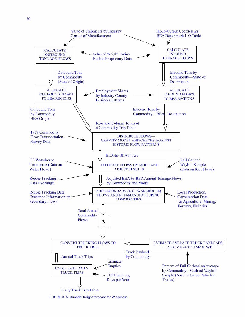
30

Value of Shipments by Industry Input–Output Coefficients Census of Manufacturers BEA Benchmark I–O Table Value of Weight Ratios Reebie Proprietary Data Outbound Tons Inbound Tons by

by Commodity Commodity—State of (State of Origin) Destination

Employment Shares by Industry County Business Patterns Outbound Tons Inbound Tons by by Commodity Commodity—BEA Destination BEA Origin Row and Column Totals of a Commodity Trip Table 1977 Commodity Flow Transportation Survey Data BEA-to-BEA Flows US Waterborne Rail Carload Commerce (Data on Waybill Sample Water Flows) (Data on Rail Flows) Reebie Trucking Adjusted BEA-to-BEA Annual Tonnage Flows Data Exchange by Commodity and Mode Reebie Trucking Data Local Production/ Exchange Information on Consumption Data Secondary Flows for Agriculture, Mining, Forestry, Fisheries Total Annual Commodity

Flows

Truck Payload Annual Truck Trips by Commodity Estimate Empties Percent of Full Carload on Average by Commodity—Carload Waybill 310 Operating Sample (Assume Same Ratio for Days per Year Trucks) Daily Truck Trip Table

FIGURE 3 Multimodal freight forecast for Wisconsin.

CALCULATE OUTBOUND

TONNAGE FLOWS

DISTRIBUTE FLOWS— GRAVITY MODEL AND CHECKS AGAINST

HISTORIC FLOW PATTERNS

ALLOCATE FLOWS BY MODE AND ADJUST RESULTS

ALLOCATE INBOUND FLOWS TO BEA REGIONS

ADD SECONDARY (E.G., WAREHOUSE) FLOWS AND NON-MANUFACTURING

COMMODITIES

ALLOCATE OUTBOUND FLOWS

TO BEA REGIONS

CALCULATE INBOUND

TONNAGE FLOWS

A

CONVERT TRUCKING FLOWS TO TRUCK TRIPS

ESTIMATE AVERAGE TRUCK PAYLOADS —ASSUME 24-TON MAX. WT.

CALCULATE DAILY TRUCK TRIPS

31

truckload trips. Factors for these additional trips were es-timated by comparing truck counts taken around truck ter-minals and truck reload facilities (e.g., warehouses) and truck trips generated from the commodity flow model. The ratio of the former to the latter was used to develop an ad-justment factor. The Second Generation Michigan Statewide Truck Travel Demand Forecasting Model, Draft for Review (Par-sons Brinckerhoff Quade & Douglas 1998)—The model uses data from the 1993 CFS and applies employment data by producing industry to estimate trip productions. The CFS was then used to estimate trip destinations, and attrac-tion rates were calculated by allocating the attractions to consuming industries using the national input–output ta-bles and then dividing by employment in these industries to get attraction rates per employee. The trip rates could then be applied to forecasted employment data to estimate trip generation forecasts New South Wales Australia 1999 (No publication cited. Information obtained through contacts with model devel-opers)—New South Wales is in the process of developing a commercial vehicle model, the heavy truck component of which is based on commodity flow techniques. Connecticut Department of Transportation (ConnDOT) (No publication cited. Information obtained in survey con-ducted for this project)—ConnDOT has done some state-wide and corridor studies where truck trips were estimated from commodity flow data (truckload equivalents based on Reebie Transearch data). Kentucky Department of Transportation (No publication cited. Information obtained in survey conducted for this project)—The Kentucky statewide truck model was devel-oped by Wilbur Smith Associates and is a commodity-based model. Trip generation is embedded within the model and is not an explicit step in the modeling process. Reebie Transearch data are used for initial commodity flows. The commodity flow data are used to estimate an initial trip table that is used to seed a matrix estimation program, calibrated to truck traffic counts. Kansas Department of Transportation (No publication cited. Information obtained in survey conducted for this project)—Kansas has developed a commodity-based truck model focused on the agricultural sectors. Florida Department of Transportation (FDOT) (No publication cited. Information obtained from survey)—FDOT contracted with Cambridge Systematics to develop a commodity-based truck forecasting model for the state. The model focuses primarily on long-distance freight movements. The focus on commodity freight addresses the large trucks moving on the Florida Intrastate Highway Sys-

tem, the shipment of commodities between regions in Flor-ida, and the shipment of freight between Florida and the rest of North America. The statewide commodity model does not address local delivery or service trucks, which are primarily regional in nature and are best modeled at the re-gional or the urban area level. Trip generation for the base year in the model is devel-oped from the Reebie Transearch database for Florida counties. Commodity flows within the state are provided with county level detail. More aggregate origin–destination regions are used outside of the state. Commodities in the Transearch database are aggregated to 14 basic commodity groupings. The VIUS is used to develop payload factors by commodity group and by length of haul groups, and these payload factors are applied to the tonnage flows to convert them to truck trips. For the forecast years, the model calculated tonnage production and attraction rates. Production equations were calculated as a function of employment in the producing industry and in most cases a single industry was identified as the producing industry. Attraction equations are also generally a function of employment for a single consuming industry. The appropriate consuming industry was deter-mined for each commodity using the Bureau of Economic Analysis’ 1996 Input–Output tables. Using the county-level inbound and outbound tonnage data from the base year Transearch data and employment by industry sector for each county, regression equations were estimated for both productions and attractions for each commodity group. The production and attraction equations are applied at the TAZ level to estimate inbound and outbounding ton-nage flows. The attraction tonnages by commodity group should be scaled to balance the production tonnages, in-cluding port tonnages developed separately. The total tonnages by commodity are subsequently dis-tributed among the origin–destination pairs, split among modes based on an incremental mode split, and truck ton-nages are converted to trucks based on payload factors that vary by distance. Consequently, because of all of these ad-ditional steps, it is inappropriate to convert the trip genera-tion rates directly to vehicle truck trips. The tonnage pro-duction and attraction equations are provided in Appendix C-13. Oregon Department of Transportation (No publication cited. Information obtained in survey conducted for this project)—Oregon has a first generation, statewide, inte-grated land-use and transportation model. This model in-corporates an input–output model of the Oregon economy and calculates truck trips based on estimates of monetary flows between each of 12 economic sectors and 122 zones. Yearly dollar flows are converted into average daily truck trips. The conversion factors were estimated from truck

32

trip intercept survey data collected at five ports of entry in Oregon and truck survey data collected by the Washington DOT. OTHER CRITICAL DATA SOURCES Over the last few years, several efforts sponsored by the federal government have produced or compiled truck trip generation data, mostly for metropolitan and statewide travel demand modeling applications. The most significant of these efforts have been

• FHWA sponsorship of the Quick Response Freight Manual (1996) and the Characteristics of Urban Freight Systems report (1995), both of which contain compilations of previously developed truck trip gen-eration rates.

• FHWA sponsorship of a Small Business Innovative Research project to develop freight destination choice, route choice, and mode choice models for state and MPO applications (being developed by JFA). Although the development of trip generation rates was not a specific requirement of this project, JFA has proposed a methodology that would include trip generation procedures based primarily on com-modity flows (similar to methods used in the SCAG model) mixed with additional trip generation factors for reload (local distribution and delivery) and non-goods movement trips (approaches that may be based on more standard trip rate estimates developed from trip diary data collected in several modeling studies across the country). This project is still in the early stages of development and no trip generation data are yet available.

In addition, the federal government (again, primarily the FHWA) has sponsored or contributed to a number of re-gional truck modeling efforts that have included develop-ment of trip generation data. The FHWA is currently sponsoring a major effort to de-velop national commodity flow data as part of a project en-titled “Multi-Modal Freight Analysis Framework.” The goal is to develop data and tools to analyze national freight movements and to assess their impacts on the national transportation network. A team of consultants including Reebie Associates, Batelle Memorial Institute, the WEFA Group, Wilbur Smith Associates, and Cambridge Sys-tematics is developing county-to-county commodity flows and forecasts, assigning these to the highway network as trucking flows, and developing techniques for assessing freight carrying capacity on the national highway network.

It is not clear the extent to which the detailed data underly-ing this analysis will be made available to practitioners outside the FHWA, but if some version of these data do become available, they will be extremely useful to those involved in commodity-based truck modeling. The U.S. Bureau of the Census also produces a number of data sets that are important in the development of trip generation data. One area where these resources have proven particularly important is in the development of truck trip generation data from commodity flow analysis. Two principal sources of data are significant in this regard: the CFS and the VIUS (formerly TIUS). The former, along with Reebie Transearch data, is the most common source for basic commodity flow data by mode. VIUS/TIUS has been used as the principal source of truck payload data that are used to convert truck tonnage information into truck trips. One area where private data sources have been impor-tant in the development of truck trip generation data is commodity flow and economic data sets. As noted in the descriptions of many of the state and regional modeling studies, Reebie Associates’ Transearch database has pro-vided the basic commodity flow data that many organiza-tions have used to develop truck trip generation by com-modity. The Reebie methodology has evolved over the last decade and now includes a wider range of commodities, a higher level of geographic detail for origins and destina-tions, and a more complete accounting of secondary truck movements (distribution traffic). The basic approach that Reebie uses to develop the Transearch data is to make use of a variety of public data sources including the Annual Survey of Manufacturers, the BEA benchmark input–output tables, the Surface Transportation Board’s Rail Car-load Waybill Sample (a sample of detailed information on rail shipments including tonnage and value by commodity and origin–destination information), the U.S. Army Corps of Engineers’ Waterborne Commerce Data series (data on waterborne shipments by port with full commodity detail), and the U.S. Bureau of the Census’ County Business Pat-terns (data on employment by industry at the county level) to derive the total freight flows and non-highway modal flows. This also provides an initial estimate of truck flows based on the residual from total commodity flows after all non-highway modes are accounted for. Reebie then uses data from a proprietary data exchange program with motor carriers to develop extensive data on truck movements, which provide information about the distribution of truck moves by type of carrier (truckload, less than truckload, and private), origin–destination, and truck payloads. This submodal detail for trucking has been used by a number of travel demand models to develop a more complete estimate of truck trips based on the type of carrier making the haul.

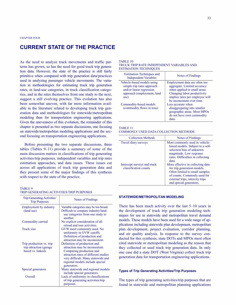
33

CHAPTER FOUR CURRENT STATE OF THE PRACTICE As the need to analyze truck movements and traffic pat-terns has grown, so has the need for good truck trip genera-tion data. However, the state of the practice is still fairly primitive when compared with trip generation data/practices used in analyzing passenger vehicle movements. The varia-tion in methodologies for estimating truck trip generation rates, in land-use categories, in truck classification catego-ries, and in the rates themselves from one study to the next, suggest a still evolving practice. This evolution has also been somewhat uneven, with far more information avail-able in the literature related to developing truck trip gen-eration data and methodologies for statewide/metropolitan modeling than for transportation engineering applications. Given the unevenness of this evolution, the remainder of this chapter is presented as two separate discussions, one focusing on statewide/metropolitan modeling applications and the sec-ond focusing on transportation engineering applications. Before presenting the two separate discussions, three tables (Tables 9–11) provide a summary of some of the main discussion matters in classifications of trip generating activities/trip purposes, independent variables and trip rates estimation approaches, and data issues. These issues cut across all applications of truck trip generation data and they present some of the major findings of this synthesis with respect to the state of the practice. TABLE 9 TRIP GENERATING ACTIVITIES/TRIP PURPOSES

Trip Generating Activities/ Trip Purposes Notes of Findings

Employment by industry (land use)

Variable categories may be too broad. Difficult to compare industry/land-

use categories from one study to another.

Commodity carried No explicit consideration of all reload and tour activities.

Truck size GVW most commonly used. No uniformity in GVW cutoffs. Definition of production and attraction may be inconsistent.

Trip production vs. trip trip attraction (garage based vs. linked)

Definition of production and attraction may be inconsistent. Comparing production and attraction rates of different studies very difficult. Many statewide and regional models include special generators.

Special generators Many statewide and regional models include special generators.

Overall Lack of uniformity in classifications of trip generating activities/trip purposes.

TABLE 10 TRUCK TRIP RATE INDEPENDENT VARIABLES AND ESTIMATION TECHNIQUES

Estimation Techniques and Independent Variables Notes of Findings

Vehicle-based models using simple trip rates approach and/or linear regression approach (employment, land use)

Employment data are often too aggregate. Limited accuracy when applied to small areas. Changing labor productivity implies rates per employee will be inconsistent over time.

Commodity-based models (commodity flows in tons)

Less accurate when disaggregating into smaller geographic areas. Most MPOs do not have own commodity data.

TABLE 11 COMMONLY USED DATA COLLECTION METHODS

Collection Methods Notes of Findings Travel diary surveys Most commonly used in vehicle-

based models. Subject to a self-selection bias of unknown magnitude. Low response rates. Difficulties in collecting data.

Intercept surveys and truck classification counts

More effective in collecting data for trip generation models. Often limited to small samples of counts. Commonly used for external trips, intercity trips and special generators.

STATEWIDE/METROPOLITAN MODELING There has been much activity over the last 5–10 years in the development of truck trip generation modeling tech-niques for use in statewide and metropolitan travel demand models. These models have been used for a wide range of ap-plications including statewide plan development, metropolitan plan development, project evaluation, corridor planning, and air quality analysis. In response to the survey con-ducted for this synthesis, state DOTs and MPOs most often cited statewide or metropolitan modeling as the reason that they collected or used truck trip generation data. In only one case did a state DOT (West Virginia) collect truck trip generation data for transportation engineering applications. Types of Trip Generating Activities/Trip Purposes The types of trip generating activities/trip purposes that are found in statewide and metropolitan planning applications

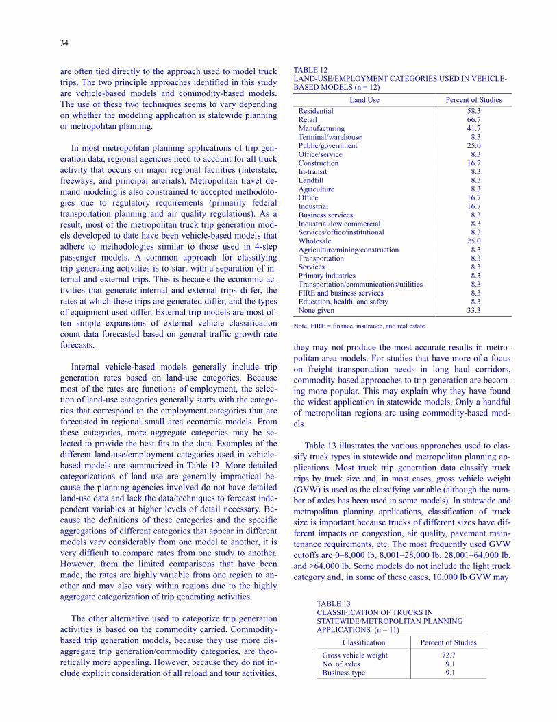
34

are often tied directly to the approach used to model truck trips. The two principle approaches identified in this study are vehicle-based models and commodity-based models. The use of these two techniques seems to vary depending on whether the modeling application is statewide planning or metropolitan planning. In most metropolitan planning applications of trip gen-eration data, regional agencies need to account for all truck activity that occurs on major regional facilities (interstate, freeways, and principal arterials). Metropolitan travel de-mand modeling is also constrained to accepted methodolo-gies due to regulatory requirements (primarily federal transportation planning and air quality regulations). As a result, most of the metropolitan truck trip generation mod-els developed to date have been vehicle-based models that adhere to methodologies similar to those used in 4-step passenger models. A common approach for classifying trip-generating activities is to start with a separation of in-ternal and external trips. This is because the economic ac-tivities that generate internal and external trips differ, the rates at which these trips are generated differ, and the types of equipment used differ. External trip models are most of-ten simple expansions of external vehicle classification count data forecasted based on general traffic growth rate forecasts. Internal vehicle-based models generally include trip generation rates based on land-use categories. Because most of the rates are functions of employment, the selec-tion of land-use categories generally starts with the catego-ries that correspond to the employment categories that are forecasted in regional small area economic models. From these categories, more aggregate categories may be se-lected to provide the best fits to the data. Examples of the different land-use/employment categories used in vehicle-based models are summarized in Table 12. More detailed categorizations of land use are generally impractical be-cause the planning agencies involved do not have detailed land-use data and lack the data/techniques to forecast inde-pendent variables at higher levels of detail necessary. Be-cause the definitions of these categories and the specific aggregations of different categories that appear in different models vary considerably from one model to another, it is very difficult to compare rates from one study to another. However, from the limited comparisons that have been made, the rates are highly variable from one region to an-other and may also vary within regions due to the highly aggregate categorization of trip generating activities. The other alternative used to categorize trip generation activities is based on the commodity carried. Commodity-based trip generation models, because they use more dis-aggregate trip generation/commodity categories, are theo-retically more appealing. However, because they do not in-clude explicit consideration of all reload and tour activities,

TABLE 12 LAND-USE/EMPLOYMENT CATEGORIES USED IN VEHICLE-BASED MODELS (n = 12)

Land Use Percent of Studies Residential 58.3 Retail 66.7 Manufacturing 41.7 Terminal/warehouse 8.3 Public/government 25.0 Office/service 8.3 Construction 16.7 In-transit 8.3 Landfill 8.3 Agriculture 8.3 Office 16.7 Industrial 16.7 Business services 8.3 Industrial/low commercial 8.3 Services/office/institutional 8.3 Wholesale 25.0 Agriculture/mining/construction 8.3 Transportation 8.3 Services 8.3 Primary industries 8.3 Transportation/communications/utilities 8.3 FIRE and business services 8.3 Education, health, and safety 8.3 None given 33.3

Note: FIRE = finance, insurance, and real estate. they may not produce the most accurate results in metro-politan area models. For studies that have more of a focus on freight transportation needs in long haul corridors, commodity-based approaches to trip generation are becom-ing more popular. This may explain why they have found the widest application in statewide models. Only a handful of metropolitan regions are using commodity-based mod-els. Table 13 illustrates the various approaches used to clas-sify truck types in statewide and metropolitan planning ap-plications. Most truck trip generation data classify truck trips by truck size and, in most cases, gross vehicle weight (GVW) is used as the classifying variable (although the num-ber of axles has been used in some models). In statewide and metropolitan planning applications, classification of truck size is important because trucks of different sizes have dif-ferent impacts on congestion, air quality, pavement main-tenance requirements, etc. The most frequently used GVW cutoffs are 0–8,000 lb, 8,001–28,000 lb, 28,001–64,000 lb, and >64,000 lb. Some models do not include the light truck category and, in some of these cases, 10,000 lb GVW may

TABLE 13 CLASSIFICATION OF TRUCKS IN STATEWIDE/METROPOLITAN PLANNING APPLICATIONS (n = 11)

Classification Percent of Studies

Gross vehicle weight 72.7 No. of axles 9.1 Business type 9.1

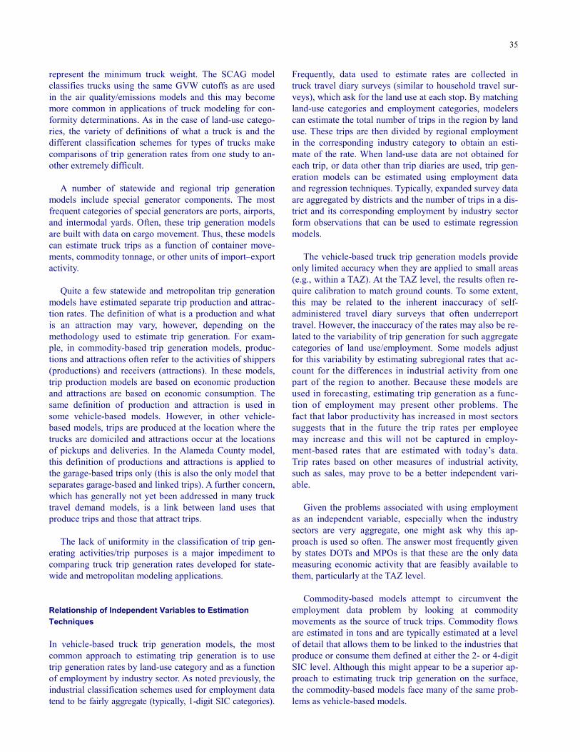
35

represent the minimum truck weight. The SCAG model classifies trucks using the same GVW cutoffs as are used in the air quality/emissions models and this may become more common in applications of truck modeling for con-formity determinations. As in the case of land-use catego-ries, the variety of definitions of what a truck is and the different classification schemes for types of trucks make comparisons of trip generation rates from one study to an-other extremely difficult. A number of statewide and regional trip generation models include special generator components. The most frequent categories of special generators are ports, airports, and intermodal yards. Often, these trip generation models are built with data on cargo movement. Thus, these models can estimate truck trips as a function of container move-ments, commodity tonnage, or other units of import–export activity. Quite a few statewide and metropolitan trip generation models have estimated separate trip production and attrac-tion rates. The definition of what is a production and what is an attraction may vary, however, depending on the methodology used to estimate trip generation. For exam-ple, in commodity-based trip generation models, produc-tions and attractions often refer to the activities of shippers (productions) and receivers (attractions). In these models, trip production models are based on economic production and attractions are based on economic consumption. The same definition of production and attraction is used in some vehicle-based models. However, in other vehicle-based models, trips are produced at the location where the trucks are domiciled and attractions occur at the locations of pickups and deliveries. In the Alameda County model, this definition of productions and attractions is applied to the garage-based trips only (this is also the only model that separates garage-based and linked trips). A further concern, which has generally not yet been addressed in many truck travel demand models, is a link between land uses that produce trips and those that attract trips. The lack of uniformity in the classification of trip gen-erating activities/trip purposes is a major impediment to comparing truck trip generation rates developed for state-wide and metropolitan modeling applications. Relationship of Independent Variables to Estimation Techniques In vehicle-based truck trip generation models, the most common approach to estimating trip generation is to use trip generation rates by land-use category and as a function of employment by industry sector. As noted previously, the industrial classification schemes used for employment data tend to be fairly aggregate (typically, 1-digit SIC categories).

Frequently, data used to estimate rates are collected in truck travel diary surveys (similar to household travel sur-veys), which ask for the land use at each stop. By matching land-use categories and employment categories, modelers can estimate the total number of trips in the region by land use. These trips are then divided by regional employment in the corresponding industry category to obtain an esti-mate of the rate. When land-use data are not obtained for each trip, or data other than trip diaries are used, trip gen-eration models can be estimated using employment data and regression techniques. Typically, expanded survey data are aggregated by districts and the number of trips in a dis-trict and its corresponding employment by industry sector form observations that can be used to estimate regression models. The vehicle-based truck trip generation models provide only limited accuracy when they are applied to small areas (e.g., within a TAZ). At the TAZ level, the results often re-quire calibration to match ground counts. To some extent, this may be related to the inherent inaccuracy of self-administered travel diary surveys that often underreport travel. However, the inaccuracy of the rates may also be re-lated to the variability of trip generation for such aggregate categories of land use/employment. Some models adjust for this variability by estimating subregional rates that ac-count for the differences in industrial activity from one part of the region to another. Because these models are used in forecasting, estimating trip generation as a func-tion of employment may present other problems. The fact that labor productivity has increased in most sectors suggests that in the future the trip rates per employee may increase and this will not be captured in employ-ment-based rates that are estimated with today’s data. Trip rates based on other measures of industrial activity, such as sales, may prove to be a better independent vari-able. Given the problems associated with using employment as an independent variable, especially when the industry sectors are very aggregate, one might ask why this ap-proach is used so often. The answer most frequently given by states DOTs and MPOs is that these are the only data measuring economic activity that are feasibly available to them, particularly at the TAZ level. Commodity-based models attempt to circumvent the employment data problem by looking at commodity movements as the source of truck trips. Commodity flows are estimated in tons and are typically estimated at a level of detail that allows them to be linked to the industries that produce or consume them defined at either the 2- or 4-digit SIC level. Although this might appear to be a superior ap-proach to estimating truck trip generation on the surface, the commodity-based models face many of the same prob-lems as vehicle-based models.

36

Generally, commodity flows are first estimated as state-to-state flows and are then disaggregated to county-to-county flows. Depending on the source of the commodity flow data, the process of geographically disaggregating the flows may involve less and less accurate data, the more geographically disaggregate the estimates become. Al-though state-to-state flow data are generally reliable for most commodities, the statistical reliability of county-to-county flow data is not well documented. In metropolitan models, these flows are further disaggregated to the TAZ level. This is usually done by allocating the origins and destinations of the flows based on employment data. Some states and MPOs have developed estimates of employment by TAZ at the 2-digit SIC level using data such as Dunn & Bradstreet or American Business Information files, which list employment for individual businesses. However, the limitations that most MPOs face when trying to estimate vehicle-based models also apply to the disaggregation of county-to-county commodity flow data. The only advan-tage of commodity flow models in these cases would seem to be that at the county-to-county or state-to-state level they are estimated based on economic production and con-sumption measures that are better indicators of truck trips than are employment-based trip rates. This is probably why the current state of the practice in statewide modeling em-phasizes commodity-based models, whereas MPOs gener-ally favor vehicle-based approaches. The MPOs using commodity-based trip generation models have tended to use them to model external trips (interregional) or as con-trol totals at the county-to-county or city-to-city level. Because most states and MPOs do not estimate their own commodity flow data, the variable that becomes most important to them in developing trip generation estimates from commodity flows is the variable used to convert commodity flows to truck trips. In most models, this is a payload factor (average pounds per truck trip for each commodity). The payload factor may be developed uniquely for the state/MPO using locally collected data or it may be developed using data from the VIUS. National or state-level VIUS data can be used. The VIUS commodity categories do not exactly match any of the standard com-modity classification systems, so a bridge must be devel-oped to these categories. VIUS does classify truck activity based on the size of the vehicle and the length of haul, so it is possible to develop a unique set of average payload factors for long-haul trucks as distinct from local trucks and for trucks of different sizes. However, as VIUS data are made more highly disaggregate, its statistical reliability suffers. Data Collection, Validity, and Challenges Table 14 summarizes the most commonly used approaches to collecting data for truck trip generation. This table illus-trates results from the survey of practitioners and the

TABLE 14 COMMONLY APPLIED DATA COLLECTION METHODS (n = 30)

Classification Percent of Studies

Trip diaries 33.3 Classification counts 23.3 Published commodity flow data 33.3 Collected commodity flow data 16.7 Shipper/carrier/special generator surveys 3.3 Intercept surveys 26.7 Published rates 3.3

literature survey when truck trip generation rates were ac-tually calculated. A number of respondents to the survey reported on truck data collection activities that were not used to calculate trip generation rates. However, these re-sults do provide another indication of the types of truck data available to a growing number of state, metropolitan, and local planning agencies. The vast majority of these respondents had vehicle classification count data (89 percent) and several had conducted intercept surveys (44 percent). With vehicle-based modeling applications, travel diary surveys are the most frequently used source of data for es-timating truck trip generation rates. All of the trip genera-tion models developed for these applications report diffi-culties in obtaining adequate responses. In most cases, potential survey participants are screened with some type of initial contact before being sent a travel diary. Because most of the reports on these models do not state how many candidates were contacted during this initial screening, it is impossible to determine what the response rates really are. The surveys are probably subject to a high degree of self-selection bias. Because there has been no systematic evaluation of these surveys, it is hard to know how impor-tant this self-selection bias is. The results of regression modeling with these data show mixed results (coefficients of determination are almost always lower than 0.75 and in some cases have been lower than 0.50). Virtually none (less than 10 percent) of the respondents to the survey con-ducted for this study indicated that they had made any at-tempt to assess the accuracy of the results of their data col-lection programs. Collecting data from travel diaries poses special prob-lems for trucking, because drivers are generally not sur-veyed directly. Approval must be obtained from dispatch-ers, fleet managers, and/or vehicle owners, who often are concerned about the impact of the survey on driver produc-tivity and the potential for disclosure of confidential busi-ness information. In addition, management is often less re-ceptive to reasonable incentives than individual drivers. A more effective approach to collecting data for truck trip generation models is to use intercept surveys and vehicle classification counts. For these approaches to be effective, it is necessary to survey all routes into and out of the area

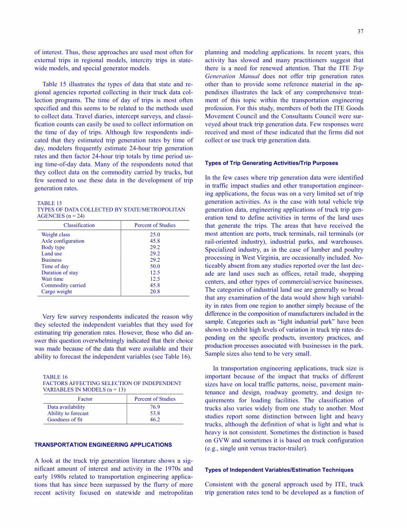
37

of interest. Thus, these approaches are used most often for external trips in regional models, intercity trips in state-wide models, and special generator models. Table 15 illustrates the types of data that state and re-gional agencies reported collecting in their truck data col-lection programs. The time of day of trips is most often specified and this seems to be related to the methods used to collect data. Travel diaries, intercept surveys, and classi-fication counts can easily be used to collect information on the time of day of trips. Although few respondents indi-cated that they estimated trip generation rates by time of day, modelers frequently estimate 24-hour trip generation rates and then factor 24-hour trip totals by time period us-ing time-of-day data. Many of the respondents noted that they collect data on the commodity carried by trucks, but few seemed to use these data in the development of trip generation rates. TABLE 15 TYPES OF DATA COLLECTED BY STATE/METROPOLITAN AGENCIES (n = 24)

Classification Percent of Studies

Weight class 25.0 Axle configuration 45.8 Body type 29.2 Land use 29.2 Business 29.2 Time of day 50.0 Duration of stay 12.5 Wait time 12.5 Commodity carried 45.8 Cargo weight 20.8

Very few survey respondents indicated the reason why they selected the independent variables that they used for estimating trip generation rates. However, those who did an-swer this question overwhelmingly indicated that their choice was made because of the data that were available and their ability to forecast the independent variables (see Table 16).

TABLE 16 FACTORS AFFECTING SELECTION OF INDEPENDENT VARIABLES IN MODELS (n = 13)

Factor Percent of Studies Data availability 76.9 Ability to forecast 53.8 Goodness of fit 46.2

TRANSPORTATION ENGINEERING APPLICATIONS A look at the truck trip generation literature shows a sig-nificant amount of interest and activity in the 1970s and early 1980s related to transportation engineering applica-tions that has since been surpassed by the flurry of more recent activity focused on statewide and metropolitan

planning and modeling applications. In recent years, this activity has slowed and many practitioners suggest that there is a need for renewed attention. That the ITE Trip Generation Manual does not offer trip generation rates other than to provide some reference material in the ap-pendixes illustrates the lack of any comprehensive treat-ment of this topic within the transportation engineering profession. For this study, members of both the ITE Goods Movement Council and the Consultants Council were sur-veyed about truck trip generation data. Few responses were received and most of these indicated that the firms did not collect or use truck trip generation data. Types of Trip Generating Activities/Trip Purposes In the few cases where trip generation data were identified in traffic impact studies and other transportation engineer-ing applications, the focus was on a very limited set of trip generation activities. As is the case with total vehicle trip generation data, engineering applications of truck trip gen-eration tend to define activities in terms of the land uses that generate the trips. The areas that have received the most attention are ports, truck terminals, rail terminals (or rail-oriented industry), industrial parks, and warehouses. Specialized industry, as in the case of lumber and poultry processing in West Virginia, are occasionally included. No-ticeably absent from any studies reported over the last dec-ade are land uses such as offices, retail trade, shopping centers, and other types of commercial/service businesses. The categories of industrial land use are generally so broad that any examination of the data would show high variabil-ity in rates from one region to another simply because of the difference in the composition of manufacturers included in the sample. Categories such as “light industrial park” have been shown to exhibit high levels of variation in truck trip rates de-pending on the specific products, inventory practices, and production processes associated with businesses in the park. Sample sizes also tend to be very small. In transportation engineering applications, truck size is important because of the impact that trucks of different sizes have on local traffic patterns, noise, pavement main-tenance and design, roadway geometry, and design re-quirements for loading facilities. The classification of trucks also varies widely from one study to another. Most studies report some distinction between light and heavy trucks, although the definition of what is light and what is heavy is not consistent. Sometimes the distinction is based on GVW and sometimes it is based on truck configuration (e.g., single unit versus tractor-trailer). Types of Independent Variables/Estimation Techniques Consistent with the general approach used by ITE, truck trip generation rates tend to be developed as a function of

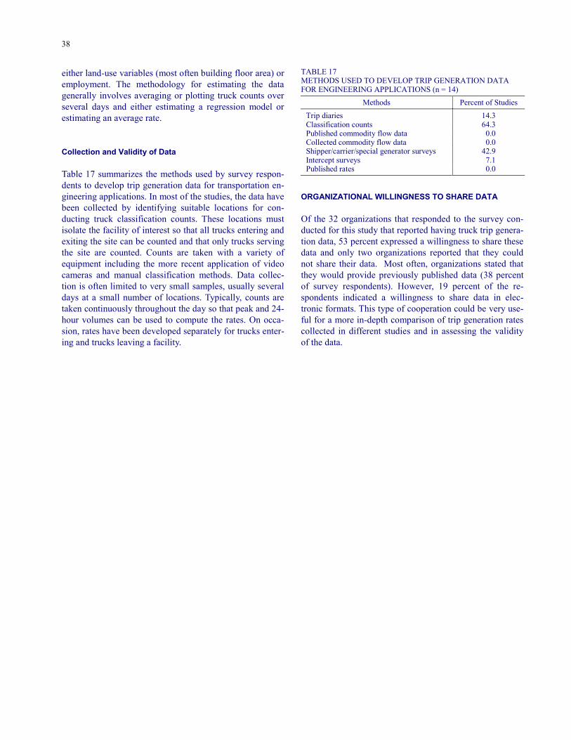
38

either land-use variables (most often building floor area) or employment. The methodology for estimating the data generally involves averaging or plotting truck counts over several days and either estimating a regression model or estimating an average rate. Collection and Validity of Data Table 17 summarizes the methods used by survey respon-dents to develop trip generation data for transportation en-gineering applications. In most of the studies, the data have been collected by identifying suitable locations for con-ducting truck classification counts. These locations must isolate the facility of interest so that all trucks entering and exiting the site can be counted and that only trucks serving the site are counted. Counts are taken with a variety of equipment including the more recent application of video cameras and manual classification methods. Data collec-tion is often limited to very small samples, usually several days at a small number of locations. Typically, counts are taken continuously throughout the day so that peak and 24-hour volumes can be used to compute the rates. On occa-sion, rates have been developed separately for trucks enter-ing and trucks leaving a facility.

TABLE 17 METHODS USED TO DEVELOP TRIP GENERATION DATA FOR ENGINEERING APPLICATIONS (n = 14)

Methods Percent of Studies

Trip diaries 14.3 Classification counts 64.3 Published commodity flow data 0.0 Collected commodity flow data 0.0 Shipper/carrier/special generator surveys 42.9 Intercept surveys 7.1 Published rates 0.0

ORGANIZATIONAL WILLINGNESS TO SHARE DATA Of the 32 organizations that responded to the survey con-ducted for this study that reported having truck trip genera-tion data, 53 percent expressed a willingness to share these data and only two organizations reported that they could not share their data. Most often, organizations stated that they would provide previously published data (38 percent of survey respondents). However, 19 percent of the re-spondents indicated a willingness to share data in elec-tronic formats. This type of cooperation could be very use-ful for a more in-depth comparison of trip generation rates collected in different studies and in assessing the validity of the data.

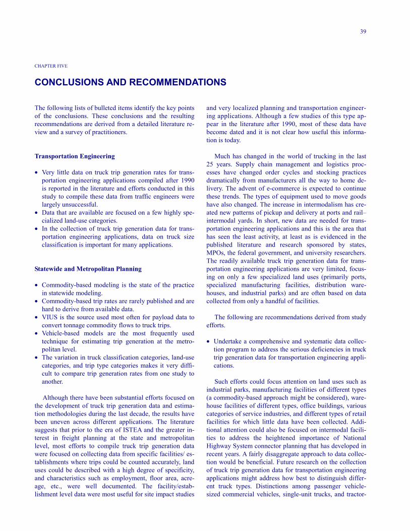
39

CHAPTER FIVE CONCLUSIONS AND RECOMMENDATIONS The following lists of bulleted items identify the key points of the conclusions. These conclusions and the resulting recommendations are derived from a detailed literature re-view and a survey of practitioners. Transportation Engineering • Very little data on truck trip generation rates for trans-

portation engineering applications compiled after 1990 is reported in the literature and efforts conducted in this study to compile these data from traffic engineers were largely unsuccessful.

• Data that are available are focused on a few highly spe-cialized land-use categories.

• In the collection of truck trip generation data for trans-portation engineering applications, data on truck size classification is important for many applications.

Statewide and Metropolitan Planning • Commodity-based modeling is the state of the practice

in statewide modeling. • Commodity-based trip rates are rarely published and are

hard to derive from available data. • VIUS is the source used most often for payload data to

convert tonnage commodity flows to truck trips. • Vehicle-based models are the most frequently used

technique for estimating trip generation at the metro-politan level.

• The variation in truck classification categories, land-use categories, and trip type categories makes it very diffi-cult to compare trip generation rates from one study to another.

Although there have been substantial efforts focused on the development of truck trip generation data and estima-tion methodologies during the last decade, the results have been uneven across different applications. The literature suggests that prior to the era of ISTEA and the greater in-terest in freight planning at the state and metropolitan level, most efforts to compile truck trip generation data were focused on collecting data from specific facilities/ es-tablishments where trips could be counted accurately, land uses could be described with a high degree of specificity, and characteristics such as employment, floor area, acre-age, etc., were well documented. The facility/estab-lishment level data were most useful for site impact studies

and very localized planning and transportation engineer-ing applications. Although a few studies of this type ap-pear in the literature after 1990, most of these data have become dated and it is not clear how useful this informa-tion is today. Much has changed in the world of trucking in the last 25 years. Supply chain management and logistics proc-esses have changed order cycles and stocking practices dramatically from manufacturers all the way to home de-livery. The advent of e-commerce is expected to continue these trends. The types of equipment used to move goods have also changed. The increase in intermodalism has cre-ated new patterns of pickup and delivery at ports and rail–intermodal yards. In short, new data are needed for trans-portation engineering applications and this is the area that has seen the least activity, at least as is evidenced in the published literature and research sponsored by states, MPOs, the federal government, and university researchers. The readily available truck trip generation data for trans-portation engineering applications are very limited, focus-ing on only a few specialized land uses (primarily ports, specialized manufacturing facilities, distribution ware-houses, and industrial parks) and are often based on data collected from only a handful of facilities. The following are recommendations derived from study efforts. • Undertake a comprehensive and systematic data collec-

tion program to address the serious deficiencies in truck trip generation data for transportation engineering appli-cations.

Such efforts could focus attention on land uses such as industrial parks, manufacturing facilities of different types (a commodity-based approach might be considered), ware-house facilities of different types, office buildings, various categories of service industries, and different types of retail facilities for which little data have been collected. Addi-tional attention could also be focused on intermodal facili-ties to address the heightened importance of National Highway System connector planning that has developed in recent years. A fairly disaggregate approach to data collec-tion would be beneficial. Future research on the collection of truck trip generation data for transportation engineering applications might address how best to distinguish differ-ent truck types. Distinctions among passenger vehicle-sized commercial vehicles, single-unit trucks, and tractor-

40

trailers could be incorporated in trip generation rates. Rates by number of axles might also be considered. Truck size is significant in the design of roadways for the prediction of axle loadings, intersection geometry, and signalization, as well as essential in terms of provision of specialized truck facilities, such as off-street loading docks or on-street load-ing zones. • As more substantial study data becomes available, the

assumption of a linear relationship between trips and such variables as employment, floor area, or acreage needs to be re-examined.

As noted previously, industrial productivity relation-ships have a strong impact on truck trips and there are a number of truck trip generating activities that exhibit economies of scale. • Focusing on truck trip generation data for transportation

engineering applications, collect data from facilities of different sizes to determine if the relationship between trip generation and independent variables such as em-ployment, floor area, and acreage is linear or best ex-pressed by some other functional form.

• Document commodity-flow approaches and produce a current state-of-the-practice manual for developing statewide truck trip generation data from commodity flows.

• Compare the truck trip generation rates per employee at the 2-digit SCTG level of detail from different state commodity-based models to determine if such rates would be transferable.

If rates are comparable, it may be possible to develop trip generation rates by commodity that could be used

across the United States without developing a unique set of commodity flow data and average payload data for each new statewide model. • A rethinking of the Vehicle Inventory and Use Survey

may be in order. The definition of major commodity could be reclassified to match the SCTG system, and sample size could be redesigned to provide sufficient samples by strata to meet the disaggregation requirements described above.

• Collect data from external roadside intercept surveys to identify the number of internal trips typically made by trucks registered outside of a region.

With data available from a number of regions across the country, it might be possible to begin to estimate the im-pact of these trips on internal trip generation models. • Research might involve the compilation of the data de-

rived from the vehicle-based trip generation models and the re-estimation of trip rates in a consistent fashion to see how variable these rates really are.

• Extend the utility of commodity-based models by con-ducting research to estimate the commodity distribution practices of different industries.

Commodity-based models can do a reasonable job of estimating the number of truck trips associated with the production end and the consumption end of commodity moves. Further investigation is needed to determine if trip generation relationships that capture distribution move-ments in between these two ends can be estimated. For ex-ample, conduct an extensive survey of distribution ware-houses to determine if a relationship exists between distribution movements and commodity groups, size of business, geographic region, etc.

41

REFERENCES Aherns, G.A., K.W. Forstall, R.U. Guthrie, and B.J. Ryan,

“Analysis of Truck Deliveries in a Small Business Dis-trict,” Transportation Research Record 637, Transporta-tion Research Board, National Research Council, Wash-ington, D.C., 1977, pp. 81–86.

Al-Deek, H.M., G. Johnson, A. Mohamed, and A. El-Maghraby, “Truck Trip Generation Models for Seaports with Container and Trailer Operation,” Transportation Research Record 1719, Transportation Research Board, National Research Council, Washington, D.C., 2000, pp. 1–9.

Black, W.R., Transport Flows in the State of Indiana: Com-modity Database Development and Traffic Assignment: Phase 2, Transportation Research Center and Department of Geography, Indiana University, Bloomington, 1997.

Brogan, J.D. and K.W. Heathington, An Analysis of Truck Travel Demand Forecasting Techniques and Data Re-quirements, University of Tennessee, Knoxville, 1977, 264 pp.

Cambridge Systematics, Portland Commodity Flow Tacti-cal Model System: Functional Specifications, Prepared for Portland Metro, Cambridge, Mass., 1998.

Cambridge Systematics, COMSIS Corporation, and Uni-versity of Wisconsin–Milwaukee, Quick Response Freight Manual, Prepared for the Federal Highway Administration, the Federal Transit Administration, the Office of the Secre-tary of Transportation, and the U.S. Environmental Pro-tection Agency, Washington, D.C., 1996.

Christiansen, D.L., Urban Transportation Planning for Goods and Services: A Reference Guide, Federal High-way Administration, Washington, D.C., 1979, 71 pp.

Cutler, M. et al., “Assessment of Market Demand for Cross-Harbor Rail Freight Service in the New York Metropolitan Region,” Transportation Research Record 1719, Transportation Research Board, National Re-search Council, Washington, D.C., 2000, pp. 17–26.

Delaware Valley Regional Planning Commission (DVRPC), Truck Trip Generation at Intermodal Facilities in the Delaware Valley Region, DVRPC, Philadelphia, Pa., 2000.

DeShazo, Tang & Associates, Inc., Trip Generation Study for Rail-Oriented Industrial Complex, Prepared for Jones & Carter, Houston, Tex., 2000.

Fischer, M., J. Ang-Olson, and A. La, “External Urban Truck Trips Based on Commodity Flows: A Model,” Transportation Research Record 1707, Transportation Research Board, National Research Council, Washing-ton, D.C., 2000, pp. 73–80.

French, L.J., R.W. Eck, and R.W. Balmer, Trip Generation Rates, Peaking Characteristics, and Vehicle Mix Char-acteristics of Special West Virginia Generators, West Virginia Department of Transportation Research Project

125, West Virginia University, Morgantown, February 2000.

French, L.J. and R.W. Eck, West Virginia Special Genera-tors Study, 68th Annual Meeting of the Institute of Transportation Engineers, Toronto, Ontario, Canada, ITE, Washington, D.C., 1980.

Gannett Fleming, Inc., Technical Memorandum No. 2: Truck/Taxi Travel Survey, Tampa, Fla., July 1993.

Greater Vancouver Regional District and Province of Brit-ish Columbia, Trucking in Greater Vancouver: Demand Forecast and Policy Implications, Transport 2021 Techni-cal Report 7, Victoria, British Columbia, Canada, 1993.

Guha, T. and C.M. Walton, “Intermodal Container Ports: Application of Automatic Vehicle Classification System for Collecting Trip Generation Data,” Transportation Research Record 1383, Transportation Research Board, National Research Council, Washington, D.C., 1993, pp. 17–23.

Habib, P.A., Curbside Pickup and Delivery Operations and Arterial Traffic Impacts, Report FHWA/RD-80/020, Prepared for the Federal Highway Administration, Of-fice of Research and Development, Washington, D.C., 1981, 134 pp.

Institute of Transportation Engineers (ITE), Trip Genera-tion, 6th ed., ITE, Washington, D.C., 1997.

Institute of Transportation Engineers (ITE), Trip Genera-tion Handbook, ITE, Washington, D.C., 1998.

Institute of Transportation Engineers (ITE) Technical Council Committee 6A-46, Truck Terminal Trip Gen-eration, ITE, Washington, D.C., 1995.

Jack Faucett Associates, Greater Buffalo–Niagara Re-gional Transportation Council Goods Movement Study, Prepared for the Greater Buffalo–Niagara Regional Transportation Council, Buffalo, N.Y., 1999.

Krishnan, V. and K. Hancock, “Highway Freight Flow As-signment in Massachusetts Using Geographic Informa-tion Systems,” Transportation Research Record 1625, Transportation Research Board, National Research Council, Washington, D.C., 1998, pp. 156–164.

Lancaster Engineering, Trip Generation Study for T.M. Lee Warehouse Distribution Center Development Proposed for N. Ramsey Boulevard in the Rivergate Area of Port-land, OR, Prepared for VLMK Consulting Engineers, Portland, Ore., November 1998.

McKinstry, D.L. and L.G. Nungesser, “Transferability of Trip Generation Rates for Selected Special Generators,” In Transportation Planning Methods Applications, Pro-ceedings, Third National Conference on Transportation Planning Methods Applications, Dallas, Tex., April 22–26, 1991, Transportation Research Board, National Re-search Council, Washington, D.C.

42

Memmott, F.W., NCHRP Report 260: Application of Statewide Freight Demand Forecasting Techniques, Transportation Research Board, National Research Council, Washington, D.C., 1983.

Meyer, Mohaddes Associates, Jack Faucett Associates, Ad-vanced Transportation Systems, Cordoba Corporation, Urban Analysis Group, and DRI/McGraw–Hill, South-ern California Association of Governments (SCAG) Heavy Duty Truck Model and VMT Estimation, Pre-pared for the SCAG, Los Angeles, October 1999.

Ogden, K.W., Urban Goods Movement: A Guide to Policy and Planning, Ashgate Publishing Co., Brookfield, Vt., 1992, 417 pp.

Park, M.-B. and R.L. Smith, Jr., “Development of a State-wide Truck–Travel Demand Model with Limited Ori-gin–Destination Survey Data,” Transportation Re-search Record 1602, Transportation Research Board, National Research Council, Washington, D.C., 1996, pp. 14–21.

Parsons Brinckerhoff Quade & Douglas, Inc., The Second Generation Michigan Statewide Truck Travel Demand Forecasting Model, Draft for Review, Prepared for the Travel Demand Analysis Section of the Michigan De-partment of Transportation, Lansing, Mich., September 21, 1998.

Rawling, F.G. and J.P. Reilly, “CATS Commercial Vehicle Survey of 1986: A Discussion of Project Management and Issues,” CATS Research News, Vol. 26, Nos. 1 and 2, 1987, pp. 5–27.

Reich, Anderson, and Drake, Baltimore Truck Trip Attraction Study, Department of Planning, City of Baltimore, Md., 1987.

Reid Crowther, Jack Faucett Associates, Cambridge Sys-tematics, and Transys International, Lower Mainland Truck Freight Study, Prepared for Translink, Vancouver, B.C., Canada, 2000.

Ruiter, E.R. and Cambridge Systematics, Development of an Urban Truck Travel Model for the Phoenix Metro-politan Area, Prepared for the Arizona Department of Transportation, Phoenix, February 1992, 91 pp.

SAIC and Harvey Consultants, Analysis of Freight Move-ments in the Puget Sound Region, Prepared for the Puget Sound Regional Council, San Diego, Calif., Sep-tember 1997.

Schlappi, M.L., R.G. Marshall, and I.T. Itamura, “Truck Travel in the San Francisco Bay Area,” Transportation Research Record 1383, Transportation Research Board, National Research Council, Washington, D.C., 1993, pp. 85–94.

Sorensen, P.C., E. Irelan, B. Winningham, and T.A. Noyes, “Skagit Countywide Air, Rail, Water, and Port Transpor-tation System Study,” Transportation Research Record 1602, Transportation Research Board, National Re-search Council, Washington, D.C., 1996, pp. 4–13.

Sorratini, J.A. and R.L. Smith, Jr., “Development of a Statewide Truck Trip Forecasting Model Based on Commodity Flows and Input-Output Coefficients,” Transportation Research Record 1707, Transportation Research Board, National Research Council, Washing-ton, D.C., 2000, pp. 49–55.

Spielberg, F. and S.A. Smith, “Service and Supply Trips at Federal Institutions in Washington, D.C. Area,” Trans-portation Research Record 834, Transportation Re-search Board, National Research Council, Washington, D.C., 1977, pp. 15–20.

Tadi, R.R. and P. Balbach, “Truck Trip Generation Charac-teristics of Nonresidential Land Uses,” ITE Journal, Vol. 64, No. 7, 1994, pp. 43–47.

Thornton, M., et al., “Development of Urban Commercial Vehicle Travel Model and Heavy-Duty Vehicle Emis-sions Model for Atlanta Region,” Presented at the 77th Annual Meeting of the Transportation Research Board, Washington, D.C., January 1998.

U.S. Bureau of the Census, Commodity Flow Survey, 1997, Washington, D.C., 1999.

U.S. Bureau of the Census, Economic Census, 1997: Cen-sus of Manufacturers and County Business Patterns, Washington, D.C., 1999.

Wegmann, F.J., A. Chatterjee, M.E. Lipinski, B.E. Jennings, and R.E. McGinnis, Characteristics of Urban Freight Systems, Federal Highway Administration, Washington, D.C., 1995, 410 pp.

Wilbur Smith Associates, BACTS Truck Route Study, Pre-pared for the Bangor Area Comprehensive Transporta-tion System, Bangor, Maine, 1998.

Wilbur Smith Associates in association with Reebie Asso-ciates, Multimodal Freight Forecasts for Wisconsin, 1996.

43

GLOSSARY Business Economic Areas (BEA)—A number of counties

grouped together for the purpose of reporting economic data. BEA regions are established by the U.S. Bureau of Economic Analysis.

Coefficient of determination (R2)—A statistical measure

computed for regression equations, the coefficient of determination measures the degree to which variation in the dependent variable is explained by the independent variables in the equation. R2 always has a value between 0 and 1. The higher the value, the more that the equation can be said to explain the variation in the dependent variable. Because the R2 value will always increase with the addition of more independent variables, a value called “adjusted R2” is often computed that does not in-crease with the addition of independent variables unless they provide increased explanatory value.

Combination vehicle—A truck that includes a separate

power unit (usually referred to as a tractor) and one or more cargo carrying units (trailers or semi-trailers). Com-bination vehicles will legally carry one or two (tandem) trailers. In some locations, triple trailers are legal.

Commodity—As used in most freight studies, commodity

refers to the cargo carried by the truck. There are sev-eral standard commodity classification systems in use in North America.

Commodity flow—A quantity of a specified commodity

moving between a specified origin and destination re-gion. Commodity quantities are usually given in terms of weight (tons) or value, and origin–destination regions are typically specified in terms of states/provinces, counties, or cities.

Commodity Flow Survey (CFS)—A survey conducted in

the United States every 5 years as part of the Economic Census. The first CFS was conducted in 1992 (com-pleted in 1993) and the second survey was conducted in 1997. The survey collects information about outbound goods shipments. Certain limitations in shipment cover-age exist and are explained in literature provided by the Bureau of Transportation Statistics and the U.S. Bureau of the Census.

Commodity-based truck models—Truck models that esti-

mate truck trip generation and trip distribution using data from commodity flow databases. Commodity flows are generally disaggregated geographically and con-verted from annual tonnage flows to daily truck traffic flows prior to assignment to a roadway network.

Distribution traffic—Truck traffic moving from a ware-house or regional distribution center to retail outlets or final consumers.

Drayage—The movement of goods, generally by truck,

from the primary shipper (or to the receiver) from the main shipment mode (e.g., goods trucked from a ship-per to a port for export). Drayage moves are generally short-haul moves made by specialized carriers.

E-commerce—Electronic commerce refers to a wide range

of business-to-business and business-to-consumer trans-actions conducted by means of the Internet or other electronic media.

Expedited delivery—A range of delivery services provided

by specialized carriers to ensure high speed and high re-liability in transportation. Services may include same day, next day, or second day delivery systems.

External trip ends—The end of a trip that occurs outside of

the region in question. Factor productivity—Factors of production include all in-

puts to the production process and factor productivity refers to the efficiency with which these factors are used to produce a unit of output. An example would be labor productivity, which refers to the units of labor required to produce a dollar of output.

Final demand—A term used in economic input–output

models to refer to the quantities of demand that are de-livered for final consumption (i.e., not used as an input for a production process).

Forty-foot equivalent unit (FEU)—A unit of measure used

for containerized cargo. Standard container sizes in-clude twenty-foot lengths (TEU) and forty-foot lengths (FEU).

Forward positioning—The placement of goods (inventory)

closer to the point of final consumption than the point of production. A logistics practice used to ensure speed of delivery to customers.

Four-step urban travel model—A standard methodology

for estimating urban travel demand. The four steps in-clude: (1) trip generation—estimating the number of trips generated by different activities/land uses in the region, (2) trip distribution—the method of linking the origins and destinations of trips, (3) mode split/choice—assignment of trips to the various modes of travel that

44

are available, and (4) assignment—the assignment of traffic volumes to network routes.

Garage-based trips—A term coined by Barton Aschman in

the Alameda County truck model to refer to trips that move from a garage location to a delivery location and then back to the garage location.

Global Positioning Systems (GPS)—A satellite-based sys-

tem of tracking the location of a transmitter/receiver. The system uses microwave communication with orbiting sat-ellites to track the whereabouts of vehicles. These sys-tems are increasingly used by trucking companies to ob-tain real-time information on the location of assets.

Gravity model—A method of estimating trip distribution in

a four-step urban travel demand model. Trips are as-signed a destination zone based on a measure of attrac-tiveness (usually a measure of the relative number of trips being attracted to the zone) and a measure of im-pedance over the network. Impedance is generally measured in terms of distance, travel time, or travel cost. Trip distribution is usually directly proportional to the attractiveness variable and inversely proportional to the impedance variable.

Gross Vehicle Weight Rating (GVWR)—A manufacturer

rating that indicates the maximum rated weight of the vehicle including all cargo and the weight of the empty vehicle. GVWR is usually a function of the vehicle sus-pension system and the power unit.

Highway Performance Monitoring System (HPMS)—A

data system maintained by each state as required by the FHWA. HPMS contains information about highway pavement condition, roadway configurations, and traffic volumes. HPMS provides ground count data for a sam-ple of roadway segments in a state that can be used to estimate vehicle miles traveled by roadway functional class.

Impedance—See gravity model. Industry production function—The specific mix of factor

inputs required to produce a unit of output from a spe-cific industry.

Input–output models—First developed by the economist

Vassily Leontif, this model uses matrix algebra to relate all of the input quantities in an economy to output lev-els. If volumes of output are known by industry, the in-put–output model can be used to estimate the amount of inputs by commodity group.

Intelligent Transportation Systems (ITS)—Advanced

transportation systems that incorporate information and

control technologies to provide traveler information and vehicle control systems.

Internal trip ends—The ends of trips that occur within the

region in question. Just-in-time inventory—A logistics practice used to mini-

mize on-site inventory for a producer. Rather than stor-ing inventory on-site to meet production demands, small shipments that meet immediate production needs are taken by the producer to reduce storage costs.

Less-than-truckload (LTL)—Shipments that do not, by

themselves, fill an over-the-road truck. Specialized LTL carriers handle these shipments. Typically, LTL carriers use smaller, “city” trucks to pick up loads from custom-ers. These loads are brought to a central sorting facility in the region and assembled into full truckloads for over-the-road movement. The process is reversed at the other end of the shipment.

Linked trips—A series of truck trips in which several

pickup and/or delivery stops are made before the truck returns to its home base.

Logistics—The practices that combine freight transporta-

tion and materials management in manufacturing and distribution enterprises.

North American Industrial Classification System

(NAICS)—A multi-tiered industrial classification sys-tem. Major industry groups are assigned a single nu-merical digit. Within each major group are more disag-gregate industry categories (2-digit, 3-digit, 4-digit, etc.).

Payload—The cargo carried by a truck. Private trucking fleet—A fleet of trucks owned by the

shipper or receiver of goods. Trucks in private fleets are not for hire by other users.

Reebie Transearch Database—A commodity flow database

developed and sold by Reebie Associates of Stamford, Connecticut. Commodity flows available from Tran-search can include either 2-digit or 4-digit STCC detail and origins and destinations can be specified for states, BEA regions, or counties. The commodity flows are de-veloped using a variety of economic data from the U.S. Bureau of Census, shipment data from the U.S. Surface Transportation Board and the U.S. Army Corps of En-gineers, and a proprietary data exchange program with trucking fleets.

Reload facilities/sites—Sites at which cargo are transferred

to another mode or stored temporarily before final

45

delivery. Typical reload sites include terminals and warehouses.

Roadside intercept survey—A survey conducted by inter-

cepting vehicles at a roadside location for the purpose of conducting a data collection interview.

Screenlines—An artificial line drawn across a set of facili-

ties that generally serve the same origin and destination subareas within a metropolitan area. Screenlines are used to validate travel demand models by comparing the predicted traffic volumes at the screenline with those obtained from traffic counts.

Secondary movements—Movements of goods from ware-

houses and distribution centers to retail outlets or final consumers.

Single-unit truck—A truck where the power unit and cargo

carrying unit are combined on a single chassis. Standard Industrial Classification (SIC)—A classification

system similar to NAICS. The SIC system was recently superceded by the NAIC system.

Standard Transportation Commodity Classification

(STCC)—A standard commodity classification system similar in structure to the NAIC system of classifying industries. The STCC system has been superceded by the STCG system.

Standard Transportation Commodity Group (STCG)—See

STCC. TEU—See FEU. Tour—A set of linked trips beginning and ending at home

base. Tractor-trailer—See combination vehicle. Traffic Analysis Zone (TAZ)—Used in urban travel demand

models as a location where trips originate and terminate. Traffic assignment—Routing of traffic in an urban travel

demand model network. Traffic assignment logic gener-

ally takes into account travel time or cost on alternative paths between origin and destination.

Travel diaries—A survey instrument used to collect infor-

mation on individual trips. Travel diaries generally ask the user to record information on each trip including starting and ending location, time of trips, distance of trips, land use at trip ends, etc.

Trip chains—See tours and linked trips. Trip length frequency distribution—A distribution showing

the frequency at which trips of different lengths are taken in a regional travel demand model.

Truckload (TL)—Full truckload shipments usually handled

by a specialized TL carrier (see LTL). Value added—An economic term referring to the value

added in a production process or service above and be-yond the costs of raw materials and supplies.

Vehicle classification counts—Traffic counts that classify

the vehicles being counted. Classification counts distin-guish trucks from automobiles and may distinguish trucks based on axle configuration, truck configuration, or body type. Vehicle classification counts can be taken manually (visual observation) or with machines.

Vehicle Inventory and Use Survey (VIUS)—A survey of

truck owners conducted every 5 years as part of the U.S. economic census. Formerly referred to as the Truck In-ventory and Use Survey (TIUS), VIUS collects infor-mation about the equipment and activity characteristics of the U.S. trucking fleet.

Vehicle-based truck models—A type of truck model that

estimates trip generation directly and uses trip genera-tion, trip distribution, and traffic assignment method-ologies similar to those used in standard urban travel demand models.

Weigh-in-motion (WIM)—A technology that allows vehi-

cles to be weighed while they move over sensors em-bedded in the pavement and does not require diverting trucks through standard weigh station scales.

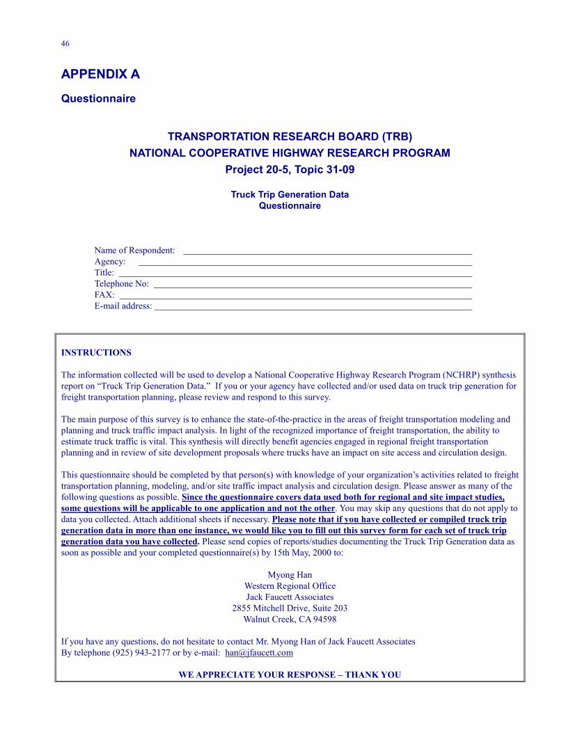
46

APPENDIX A Questionnaire

TRANSPORTATION RESEARCH BOARD (TRB) NATIONAL COOPERATIVE HIGHWAY RESEARCH PROGRAM

Project 20-5, Topic 31-09

Truck Trip Generation Data Questionnaire

Name of Respondent: Agency: Title: Telephone No: FAX: E-mail address: INSTRUCTIONS The information collected will be used to develop a National Cooperative Highway Research Program (NCHRP) synthesis report on “Truck Trip Generation Data.” If you or your agency have collected and/or used data on truck trip generation for freight transportation planning, please review and respond to this survey. The main purpose of this survey is to enhance the state-of-the-practice in the areas of freight transportation modeling and planning and truck traffic impact analysis. In light of the recognized importance of freight transportation, the ability to estimate truck traffic is vital. This synthesis will directly benefit agencies engaged in regional freight transportation planning and in review of site development proposals where trucks have an impact on site access and circulation design. This questionnaire should be completed by that person(s) with knowledge of your organization’s activities related to freight transportation planning, modeling, and/or site traffic impact analysis and circulation design. Please answer as many of the following questions as possible. Since the questionnaire covers data used both for regional and site impact studies, some questions will be applicable to one application and not the other. You may skip any questions that do not apply to data you collected. Attach additional sheets if necessary. Please note that if you have collected or compiled truck trip generation data in more than one instance, we would like you to fill out this survey form for each set of truck trip generation data you have collected. Please send copies of reports/studies documenting the Truck Trip Generation data as soon as possible and your completed questionnaire(s) by 15th May, 2000 to:

Myong Han Western Regional Office Jack Faucett Associates

2855 Mitchell Drive, Suite 203 Walnut Creek, CA 94598

If you have any questions, do not hesitate to contact Mr. Myong Han of Jack Faucett Associates By telephone (925) 943-2177 or by e-mail: han@jfaucett.com

WE APPRECIATE YOUR RESPONSE – THANK YOU

47

PART I: General & TTG Data Collection (Questions 1 through 7). 1. Have you used truck trip generation (TTG) data that was collected during the last ten years for any of the following applications (check all that apply)? Please provide name/title of your study/project you used/collected TTG data for. Please fill out form for each data source � Regional and/or sub-regional modeling � Statewide modeling � Site access and circulation design � Sizing of loading dock facilities � Curbside loading space allocation � Corridor and MIS � Inventories � Other (Please describe) 2. Did your organization collect (or fund the collection of) the TTG data you used? � Yes (Go to Question #3) � No – What was the source? _____________________________________ – Please provide contact info. If available: _______________________ _______________________ – Go to Question #4 3. If you hired a firm to collect the data for you please provide name and contact information. 4. What was the source of the funding for your data collection effort? And, what sources of funding are available to you to update/upgrade your data? 5. How was truck trip data collected?

��Trip diary survey or travel log ��Shipper/receiver survey ��Intercept survey ��Manual vehicle classification counts ��Automatic vehicle counts ��Video ��Other (Please describe) ________________________________________________________

6. What types of data were collected about truck trips? Indicate the classification system used for each box checked or provide a copy of your questionnaire/code sheet.

��Truck weight class: ��Axle configuration: ��Body type: ��Land use at trip origin/destination: ��Business/industry at trip origin/destination: ��Time of day (i.e., hour:min. / day of week / peak v. off-peak) ��Duration of stay at the site:

48

��Wait time at the site: ��Commodity carried: ��Cargo weight: ��Other (Please describe)

7. How was data geo-referenced?

��Street address ��Traffic Analysis Zone (TAZ) or other zones ��x-y coordinates ��Zip codes ��City ��County ��Other (Please describe) ��Not applicable

PART II: Data Sampling & Quality of Data (Questions 8 through 12). Note—some questions in this section may not be applicable to all respondents. Data sampling may not be applicable to trip generation data developed from counts and used for site impact analysis. Please take a moment to review all questions, and feel free to skip this section if it does not apply to your experience, or mark “not applicable” when answering the questions that are not applicable to you. 8. How was sample selected and what was the source of the sampling frame?

��Department of Motor Vehicles (DMV) registration files ��International Registration Plan (IRP) registration files ��Private fleet directories ��Business directories ��Yellow pages ��Trade association membership lists ��Freight advisory committee or steering committee ��Random roadside selection ��Other (Please describe) ��Not applicable

9. How was sample stratified? (indicate strata)

��Truck size: ��Fleet size: ��Business type: ��Geographic boundaries: ��External trips vs. internal trips: ��Other (Please describe) ��No sample / Not stratified

10. What was your sample size (number and % of population)? When providing the number of respondents, please indicate the units (e.g., trucks, fleets, trips) Number: ________ % of population: _________%

��Not applicable 11. What was response rate (number and % of population)? Number: ________ % of population: _________%

��Not applicable

49

11(a). Percentage of the collected data that were actually useable? __________%

��Not applicable 11(b). What factors had the greatest positive and negative impacts on your response and quality of data? Positive Factor: Negative Factor: 12. Was there any noticeable response bias by the following strata? Please describe the direction of bias.

��Truck size: ��Fleet size: ��Business type: ��Geographic boundaries: ��External trips vs. internal trips: ��Other (Please describe) ��No sample / Not stratified

Part III: Trip Generation Rates, Equations (Questions 13 through 15). Note—some questions in this section may not be applicable to all respondents. Please take a moment to review all questions, and feel free to skip or mark “not applicable” when answering the questions that are not applicable to you. 13. What categories of truck trips were trip rates/equations calculated for (provide categories)?

��Land use types: ��Business/industry types: ��Special generators (e.g., ports, truck terminals, event centers): ��Truck size categories (weight, axle): ��Commodity type (including non-goods movement): ��Empty vs. loaded: ��Garage-based vs. linked: ��Separate production and attraction rates: ��Activity type (e.g., pickup, delivery, fueling): ��Other (Please describe)

14. What independent variables were used to calculate trip generation rates/eqns. (describe categories)?

��Employment: ��Land use (sq. footage of building space, acres): ��Commodity flow data: ��Business output measures (e.g., shipping units): ��Sales:

50

15. Why did you select this (these) variable(s) and the level of detail in describing the variable?

��Data availability ��Ability to forecast data ��Goodness of fit to survey results ��Other (Please describe)

15(a). Please use the space below to elaborate on your choice of variables. (Attach additional sheets if necessary.) 15(b). Are there any other variables that you think would provide greater explanatory power than those you used? Please explain why you were unable to use these variables. Part IV: TTG Data Validity (Questions 16 through 20). Note—some questions in this section may not be applicable to all respondents. Please take a moment to review all questions, and feel free to skip or mark “not applicable” when answering the questions that are not applicable to you. 16. Did you use any other published data sets to condition (or to estimate) your survey data/control totals?

��Truck Inventory and Use Survey (TIUS) ��Commodity Flow Survey (CFS) ��Reebie Transearch ��Carload Waybill sample ��Army Corps of Engineers Waterborne Commerce ��Port Import Export Reporting Service (PIERS) ��Private economic forecasts ��Other (Please describe)

17. How were data expanded? (provide the name of the source for each)

��Vehicle population data ��Ground counts ��Economic data (employment, sales) ��Commodity flow control totals ��No, data were not expanded

18. How were trip generation rates/equations estimated (please provide results, attaching additional sheets if necessary)?

��Regression ��Trip rates ��Other (Please describe)

19. Did you measure accuracy and precision of results? (e.g., coefficient of variation, variance, R2) Provide results. (Attach additional sheets if necessary.)

51

20. Did you validate and/or calibrate results? Please describe process. (Attach additional sheets if necessary.) Part V: Data Sharing/Availability & Other Issues (Questions 21 through 25). Note—some questions in this section may not be applicable to all respondents. Please take a brief moment to review all questions, and feel free to skip or mark “not applicable” when answering the questions that are not applicable to you. 21. In what format is data stored?

��Electronic raw data files ��Electronic response forms ��Electronic summaries ��Tabulated summaries ��Hard copy response forms

22. Would you be willing and able to share data with others?

��Reports ��Data summaries ��Electronic data files ��Raw data files ��No, not willing / able to share data

23. How effective was the private sector involved in your data collection program? Please rank effectiveness of the private sector involvement using scale of “1” to “5” with “5” being “very effective.”

not helpful

1

2

3

4

very effective

5 Special steering committee Standing freight advisory committee Trade groups Public meetings One-on-one meetings with businesses

24. What issues do you think are most significant for advancing the state-of-the practice in truck trip generation data? Use space below to describe these issues. 25. Do you know of any other organizations that may have collected truck trip generation data or commercial vehicle studies that you would recommend we contact? Please provide name and contact information. Reminder: Please don’t forget to send us copies of available data and reports/studies if you are able to share them with us.

Thank you

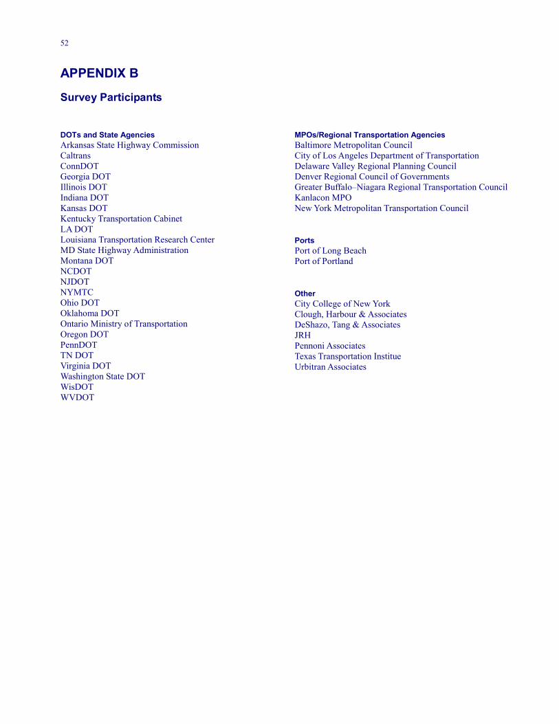
52

APPENDIX B Survey Participants DOTs and State Agencies Arkansas State Highway Commission Caltrans ConnDOT Georgia DOT Illinois DOT Indiana DOT Kansas DOT Kentucky Transportation Cabinet LA DOT Louisiana Transportation Research Center MD State Highway Administration Montana DOT NCDOT NJDOT NYMTC Ohio DOT Oklahoma DOT Ontario Ministry of Transportation Oregon DOT PennDOT TN DOT Virginia DOT Washington State DOT WisDOT WVDOT

MPOs/Regional Transportation Agencies Baltimore Metropolitan Council City of Los Angeles Department of Transportation Delaware Valley Regional Planning Council Denver Regional Council of Governments Greater Buffalo–Niagara Regional Transportation Council Kanlacon MPO New York Metropolitan Transportation Council Ports Port of Long Beach Port of Portland Other City College of New York Clough, Harbour & Associates DeShazo, Tang & Associates JRH Pennoni Associates Texas Transportation Institue Urbitran Associates

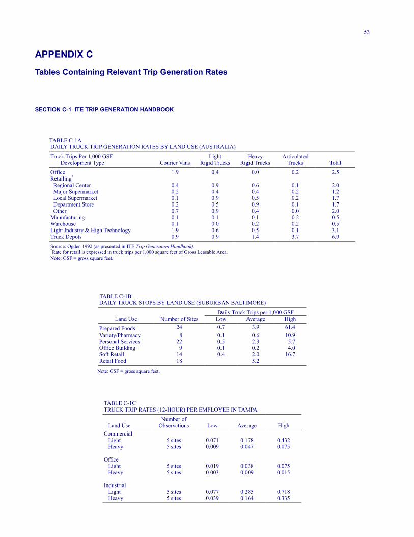
53

APPENDIX C Tables Containing Relevant Trip Generation Rates SECTION C-1 ITE TRIP GENERATION HANDBOOK TABLE C-1A

DAILY TRUCK TRIP GENERATION RATES BY LAND USE (AUSTRALIA) Truck Trips Per 1,000 GSF Light Heavy Articulated Development Type Courier Vans Rigid Trucks Rigid Trucks Trucks Total

Office 1.9 0.4 0.0 0.2 2.5 Retailing* Regional Center 0.4 0.9 0.6 0.1 2.0 Major Supermarket 0.2 0.4 0.4 0.2 1.2 Local Supermarket 0.1 0.9 0.5 0.2 1.7 Department Store 0.2 0.5 0.9 0.1 1.7 Other 0.7 0.9 0.4 0.0 2.0 Manufacturing 0.1 0.1 0.1 0.2 0.5 Warehouse 0.1 0.0 0.2 0.2 0.5 Light Industry & High Technology 1.9 0.6 0.5 0.1 3.1 Truck Depots 0.9 0.9 1.4 3.7 6.9

Source: Ogden 1992 (as presented in ITE Trip Generation Handbook). *Rate for retail is expressed in truck trips per 1,000 square feet of Gross Leasable Area. Note: GSF = gross square feet.

TABLE C-1B

DAILY TRUCK STOPS BY LAND USE (SUBURBAN BALTIMORE) Daily Truck Trips per 1,000 GSF

Land Use Number of Sites Low Average High Prepared Foods 24 0.7 3.9 61.4 Variety/Pharmacy 8 0.1 0.6 10.9 Personal Services 22 0.5 2.3 5.7 Office Building 9 0.1 0.2 4.0 Soft Retail 14 0.4 2.0 16.7 Retail Food 18 5.2

Note: GSF = gross square feet. TABLE C-1C

TRUCK TRIP RATES (12-HOUR) PER EMPLOYEE IN TAMPA Number of

Land Use Observations Low Average High Commercial Light 5 sites 0.071 0.178 0.432 Heavy 5 sites 0.009 0.047 0.075 Office Light 5 sites 0.019 0.038 0.075 Heavy 5 sites 0.003 0.009 0.015 Industrial Light 5 sites 0.077 0.285 0.718 Heavy 5 sites 0.039 0.164 0.335

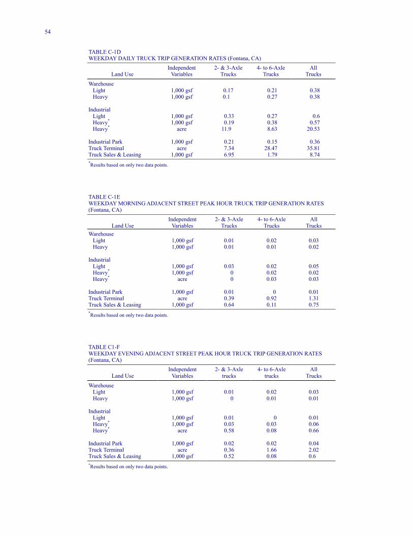
54

TABLE C-1D WEEKDAY DAILY TRUCK TRIP GENERATION RATES (Fontana, CA)

Independent 2- & 3-Axle 4- to 6-Axle All Land Use Variables Trucks Trucks Trucks

Warehouse Light 1,000 gsf 0.17 0.21 0.38 Heavy 1,000 gsf 0.1 0.27 0.38 Industrial Light 1,000 gsf 0.33 0.27 0.6 Heavy* 1,000 gsf 0.19 0.38 0.57 Heavy* acre 11.9 8.63 20.53 Industrial Park 1,000 gsf 0.21 0.15 0.36 Truck Terminal acre 7.34 28.47 35.81 Truck Sales & Leasing 1,000 gsf 6.95 1.79 8.74 *Results based on only two data points. TABLE C-1E WEEKDAY MORNING ADJACENT STREET PEAK HOUR TRUCK TRIP GENERATION RATES (Fontana, CA)

Independent 2- & 3-Axle 4- to 6-Axle All Land Use Variables Trucks Trucks Trucks

Warehouse Light 1,000 gsf 0.01 0.02 0.03 Heavy 1,000 gsf 0.01 0.01 0.02 Industrial Light 1,000 gsf 0.03 0.02 0.05 Heavy* 1,000 gsf 0 0.02 0.02 Heavy* acre 0 0.03 0.03 Industrial Park 1,000 gsf 0.01 0 0.01 Truck Terminal acre 0.39 0.92 1.31 Truck Sales & Leasing 1,000 gsf 0.64 0.11 0.75 *Results based on only two data points. TABLE C1-F WEEKDAY EVENING ADJACENT STREET PEAK HOUR TRUCK TRIP GENERATION RATES (Fontana, CA)

Independent 2- & 3-Axle 4- to 6-Axle All Land Use Variables trucks trucks Trucks

Warehouse Light 1,000 gsf 0.01 0.02 0.03 Heavy 1,000 gsf 0 0.01 0.01 Industrial Light 1,000 gsf 0.01 0 0.01 Heavy* 1,000 gsf 0.03 0.03 0.06 Heavy* acre 0.58 0.08 0.66 Industrial Park 1,000 gsf 0.02 0.02 0.04 Truck Terminal acre 0.36 1.66 2.02 Truck Sales & Leasing 1,000 gsf 0.52 0.08 0.6 *Results based on only two data points.

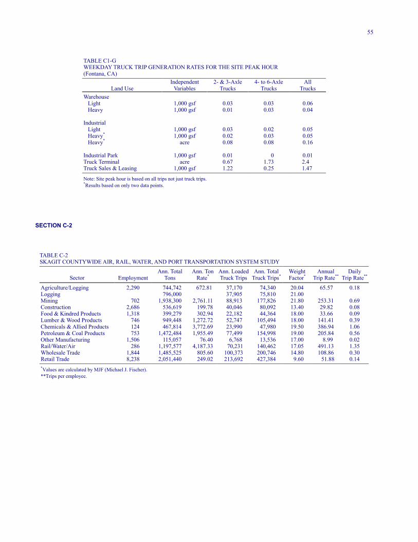
55

TABLE C1-G WEEKDAY TRUCK TRIP GENERATION RATES FOR THE SITE PEAK HOUR (Fontana, CA)

Independent 2- & 3-Axle 4- to 6-Axle All Land Use Variables Trucks Trucks Trucks

Warehouse Light 1,000 gsf 0.03 0.03 0.06 Heavy 1,000 gsf 0.01 0.03 0.04 Industrial Light 1,000 gsf 0.03 0.02 0.05 Heavy* 1,000 gsf 0.02 0.03 0.05 Heavy* acre 0.08 0.08 0.16 Industrial Park 1,000 gsf 0.01 0 0.01 Truck Terminal acre 0.67 1.73 2.4 Truck Sales & Leasing 1,000 gsf 1.22 0.25 1.47

Note: Site peak hour is based on all trips not just truck trips. *Results based on only two data points.

SECTION C-2 TABLE C-2 SKAGIT COUNTYWIDE AIR, RAIL, WATER, AND PORT TRANSPORTATION SYSTEM STUDY

Ann. Total Ann. Ton Ann. Loaded Ann. Total Weight Annual Daily Sector Employment Tons Rate* Truck Trips Truck Trips* Factor* Trip Rate** Trip Rate**

Agriculture/Logging 2,290 744,742 672.81 37,170 74,340 20.04 65.57 0.18 Logging 796,000 37,905 75,810 21.00 Mining 702 1,938,300 2,761.11 88,913 177,826 21.80 253.31 0.69 Construction 2,686 536,619 199.78 40,046 80,092 13.40 29.82 0.08 Food & Kindred Products 1,318 399,279 302.94 22,182 44,364 18.00 33.66 0.09 Lumber & Wood Products 746 949,448 1,272.72 52,747 105,494 18.00 141.41 0.39 Chemicals & Allied Products 124 467,814 3,772.69 23,990 47,980 19.50 386.94 1.06 Petroleum & Coal Products 753 1,472,484 1,955.49 77,499 154,998 19.00 205.84 0.56 Other Manufacturing 1,506 115,057 76.40 6,768 13,536 17.00 8.99 0.02 Rail/Water/Air 286 1,197,577 4,187.33 70,231 140,462 17.05 491.13 1.35 Wholesale Trade 1,844 1,485,525 805.60 100,373 200,746 14.80 108.86 0.30 Retail Trade 8,238 2,051,440 249.02 213,692 427,384 9.60 51.88 0.14 *Values are calculated by MJF (Michael J. Fischer). **Trips per employee.

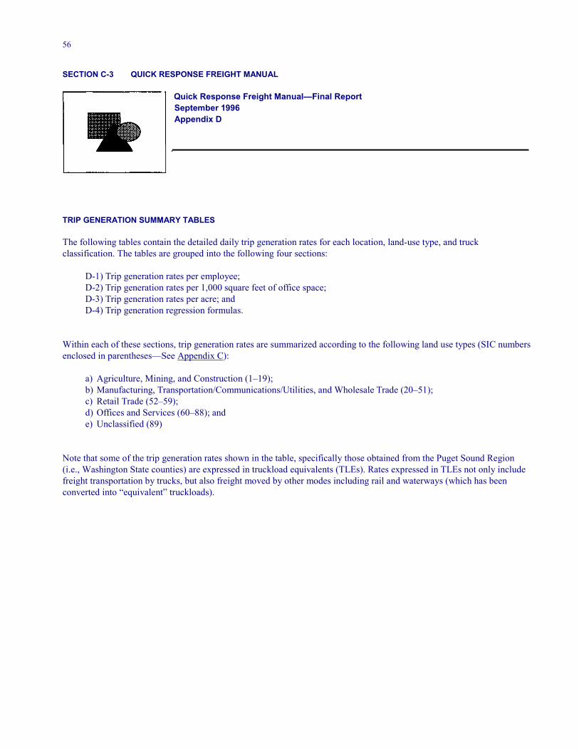
56

SECTION C-3 QUICK RESPONSE FREIGHT MANUAL

Quick Response Freight Manual—Final Report September 1996 Appendix D

TRIP GENERATION SUMMARY TABLES The following tables contain the detailed daily trip generation rates for each location, land-use type, and truck classification. The tables are grouped into the following four sections:

D-1) Trip generation rates per employee; D-2) Trip generation rates per 1,000 square feet of office space; D-3) Trip generation rates per acre; and D-4) Trip generation regression formulas.

Within each of these sections, trip generation rates are summarized according to the following land use types (SIC numbers enclosed in parentheses—See Appendix C):

a) Agriculture, Mining, and Construction (1–19); b) Manufacturing, Transportation/Communications/Utilities, and Wholesale Trade (20–51); c) Retail Trade (52–59); d) Offices and Services (60–88); and e) Unclassified (89)

Note that some of the trip generation rates shown in the table, specifically those obtained from the Puget Sound Region (i.e., Washington State counties) are expressed in truckload equivalents (TLEs). Rates expressed in TLEs not only include freight transportation by trucks, but also freight moved by other modes including rail and waterways (which has been converted into “equivalent” truckloads).

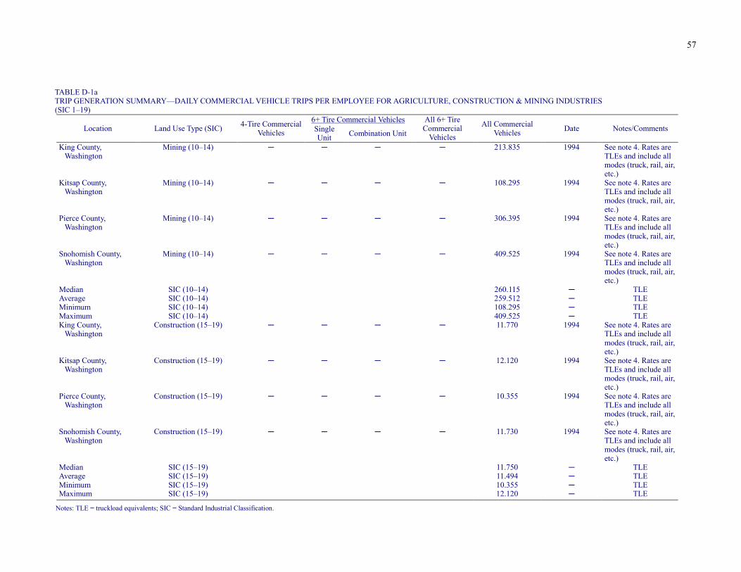
57

TABLE D-1a TRIP GENERATION SUMMARY—DAILY COMMERCIAL VEHICLE TRIPS PER EMPLOYEE FOR AGRICULTURE, CONSTRUCTION & MINING INDUSTRIES (SIC 1–19)

6+ Tire Commercial Vehicles Location Land Use Type (SIC) 4-Tire Commercial

Vehicles Single Unit Combination Unit

All 6+ Tire Commercial

Vehicles

All Commercial Vehicles Date Notes/Comments

King County, Washington

Mining (10–14) ─ ─ ─ ─ 213.835 1994 See note 4. Rates are TLEs and include all modes (truck, rail, air, etc.)

Kitsap County, Washington

Mining (10–14) ─ ─ ─ ─ 108.295 1994 See note 4. Rates are TLEs and include all modes (truck, rail, air, etc.)

Pierce County, Washington

Mining (10–14) ─ ─ ─ ─ 306.395 1994 See note 4. Rates are TLEs and include all modes (truck, rail, air, etc.)

Snohomish County, Washington

Mining (10–14) ─ ─ ─ ─ 409.525 1994 See note 4. Rates are TLEs and include all modes (truck, rail, air, etc.)

Median SIC (10–14) 260.115 ─ TLE Average SIC (10–14) 259.512 ─ TLE Minimum SIC (10–14) 108.295 ─ TLE Maximum SIC (10–14) 409.525 ─ TLE King County,

Washington Construction (15–19) ─ ─ ─ ─ 11.770 1994 See note 4. Rates are

TLEs and include all modes (truck, rail, air, etc.)

Kitsap County, Washington

Construction (15–19) ─ ─ ─ ─ 12.120 1994 See note 4. Rates are TLEs and include all modes (truck, rail, air, etc.)

Pierce County, Washington

Construction (15–19) ─ ─ ─ ─ 10.355 1994 See note 4. Rates are TLEs and include all modes (truck, rail, air, etc.)

Snohomish County, Washington

Construction (15–19) ─ ─ ─ ─ 11.730 1994 See note 4. Rates are TLEs and include all modes (truck, rail, air, etc.)

Median SIC (15–19) 11.750 ─ TLE Average SIC (15–19) 11.494 ─ TLE Minimum SIC (15–19) 10.355 ─ TLE Maximum SIC (15–19) 12.120 ─ TLE

Notes: TLE = truckload equivalents; SIC = Standard Industrial Classification.

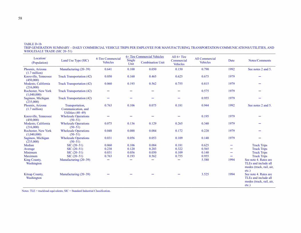
58

TABLE D-1b TRIP GENERATION SUMMARY—DAILY COMMERCIAL VEHICLE TRIPS PER EMPLOYEE FOR MANUFACTURING, TRANSPORTATION/COMMUNICATIONS/UTILITIES, AND WHOLESALE TRADE (SIC 20–51)

6+ Tire Commercial Vehicles Location/ (Population)

Land Use Type (SIC) 4-Tire Commercial Vehicles Single

Unit Combination Unit

All 6+ Tire Commercial

Vehicles

All Commercial Vehicles Date Notes/Comments

Phoenix, Arizona

(1.7 million) Manufacturing (20–39) 0.641 0.100 0.050 0.150 0.790 1992 See notes 2 and 5.

Knoxville, Tennessee (450,000)

Truck Transportation (42) 0.050 0.160 0.465 0.625 0.675 1979 ─

Modesto, California (216,000)

Truck Transportation (42) 0.060 0.193 0.562 0.755 0.815 1979 ─

Rochester, New York (1,040,000)

Truck Transportation (42) ─ ─ ─ ─ 0.575 1979 ─

Saginaw, Michigan (235,000)

Truck Transportation (42) ─ ─ ─ ─ 0.955 1979 ─

Phoenix, Arizona (1.7 million)

Transportation, Communication, and

Utilities (40–49)

0.763 0.106 0.075 0.181 0.944 1992 See notes 2 and 5.

Knoxville, Tennessee (450,000)

Wholesale Operations (50–51)

─ ─ ─ ─ 0.195 1979 ─

Modesto, California (216,000)

Wholesale Operations (50–51)

0.075 0.136 0.129 0.265 0.340 1979 ─

Rochester, New York (1,040,000)

Wholesale Operations (50–51)

0.048 0.088 0.084 0.172 0.220 1979 ─

Saginaw, Michigan (235,000)

Wholesale Operations (50–51)

0.031 0.056 0.053 0.109 0.140 1979 ─

Median SIC (20–51) 0.060 0.106 0.084 0.181 0.625 ─ Truck Trips Average SIC (20–51) 0.238 0.120 0.203 0.322 0.565 ─ Truck Trips Minimum SIC (20–51) 0.031 0.056 0.050 0.109 0.140 ─ Truck Trips Maximum SIC (20–51) 0.763 0.193 0.562 0.755 0.955 ─ Truck Trips King County,

Washington Manufacturing (20–39) ─ ─ ─ ─ 5.580 1994 See note 4. Rates are

TLEs and include all modes (truck, rail, air, etc.)

Kitsap County, Washington

Manufacturing (20–39) ─ ─ ─ ─ 3.525 1994 See note 4. Rates are TLEs and include all modes (truck, rail, air, etc.)

Notes: TLE = truckload equivalents; SIC = Standard Industrial Classification.

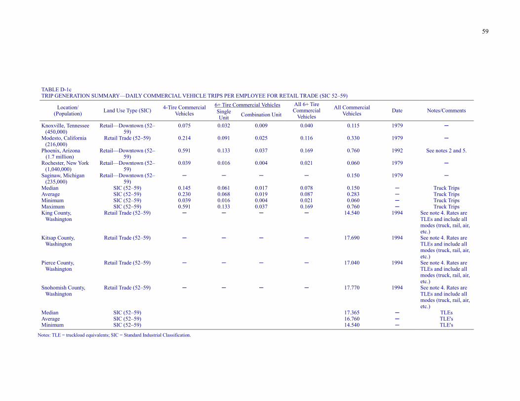
59

TABLE D-1c TRIP GENERATION SUMMARY—DAILY COMMERCIAL VEHICLE TRIPS PER EMPLOYEE FOR RETAIL TRADE (SIC 52–59)

6+ Tire Commercial Vehicles Location/ (Population) Land Use Type (SIC) 4-Tire Commercial

Vehicles Single Unit Combination Unit

All 6+ Tire Commercial

Vehicles

All Commercial Vehicles

Date

Notes/Comments

Knoxville, Tennessee

(450,000) Retail—Downtown (52–

59) 0.075 0.032 0.009 0.040 0.115 1979 ─

Modesto, California (216,000)

Retail Trade (52–59) 0.214 0.091 0.025 0.116 0.330 1979 ─

Phoenix, Arizona (1.7 million)

Retail—Downtown (52–59)

0.591 0.133 0.037 0.169 0.760 1992 See notes 2 and 5.

Rochester, New York (1,040,000)

Retail—Downtown (52–59)

0.039 0.016 0.004 0.021 0.060 1979 ─

Saginaw, Michigan (235,000)

Retail—Downtown (52–59)

─ ─ ─ ─ 0.150 1979 ─

Median SIC (52–59) 0.145 0.061 0.017 0.078 0.150 ─ Truck Trips Average SIC (52–59) 0.230 0.068 0.019 0.087 0.283 ─ Truck Trips Minimum SIC (52–59) 0.039 0.016 0.004 0.021 0.060 ─ Truck Trips Maximum SIC (52–59) 0.591 0.133 0.037 0.169 0.760 ─ Truck Trips King County,

Washington Retail Trade (52–59) ─ ─ ─ ─ 14.540 1994 See note 4. Rates are

TLEs and include all modes (truck, rail, air, etc.)

Kitsap County, Washington

Retail Trade (52–59) ─ ─ ─ ─ 17.690 1994 See note 4. Rates are TLEs and include all modes (truck, rail, air, etc.)

Pierce County, Washington

Retail Trade (52–59) ─ ─ ─ ─ 17.040 1994 See note 4. Rates are TLEs and include all modes (truck, rail, air, etc.)

Snohomish County, Washington

Retail Trade (52–59) ─ ─ ─ ─ 17.770 1994 See note 4. Rates are TLEs and include all modes (truck, rail, air, etc.)

Median SIC (52–59) 17.365 ─ TLEs Average SIC (52–59) 16.760 ─ TLE's Minimum SIC (52–59) 14.540 ─ TLE's

Notes: TLE = truckload equivalents; SIC = Standard Industrial Classification.

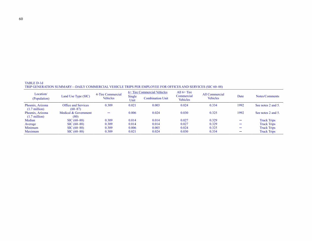
60

TABLE D-1d TRIP GENERATION SUMMARY—DAILY COMMERCIAL VEHICLE TRIPS PER EMPLOYEE FOR OFFICES AND SERVICES (SIC 60–88)

6+ Tire Commercial Vehicles Location/ (Population)

Land Use Type (SIC) 4-Tire Commercial Vehicles Single

Unit Combination Unit

All 6+ Tire Commercial

Vehicles All Commercial

Vehicles Date Notes/Comments

Phoenix, Arizona

(1.7 million) Office and Services

(60–87) 0.309 0.021 0.003 0.024 0.334 1992 See notes 2 and 5.

Phoenix, Arizona (1.7 million)

Medical & Government (80)

─ 0.006 0.024 0.030 0.325 1992 See notes 2 and 5.

Median SIC (60–88) 0.309 0.014 0.014 0.027 0.329 ─ Truck Trips Average SIC (60–88) 0.309 0.014 0.014 0.027 0.329 ─ Truck Trips Minimum SIC (60–88) 0.309 0.006 0.003 0.024 0.325 ─ Truck Trips Maximum SIC (60–88) 0.309 0.021 0.024 0.030 0.334 ─ Truck Trips

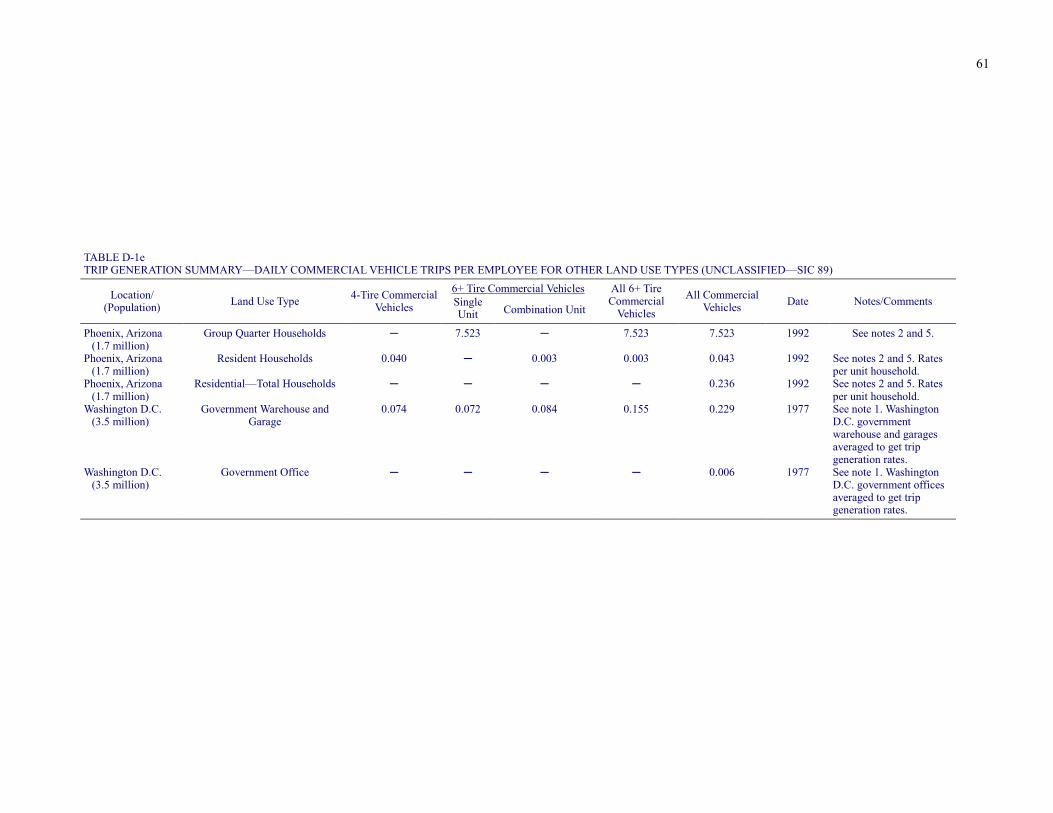
61

TABLE D-1e TRIP GENERATION SUMMARY—DAILY COMMERCIAL VEHICLE TRIPS PER EMPLOYEE FOR OTHER LAND USE TYPES (UNCLASSIFIED—SIC 89)

6+ Tire Commercial Vehicles Location/ (Population) Land Use Type 4-Tire Commercial

Vehicles Single Unit Combination Unit

All 6+ Tire Commercial

Vehicles

All Commercial Vehicles Date Notes/Comments

Phoenix, Arizona

(1.7 million) Group Quarter Households ─ 7.523 ─ 7.523 7.523 1992 See notes 2 and 5.

Phoenix, Arizona (1.7 million)

Resident Households 0.040 ─ 0.003 0.003 0.043 1992 See notes 2 and 5. Rates per unit household.

Phoenix, Arizona (1.7 million)

Residential—Total Households ─ ─ ─ ─ 0.236 1992 See notes 2 and 5. Rates per unit household.

Washington D.C. (3.5 million)

Government Warehouse and Garage

0.074 0.072 0.084 0.155 0.229 1977 See note 1. Washington D.C. government warehouse and garages averaged to get trip generation rates.

Washington D.C. (3.5 million)

Government Office ─ ─ ─ ─ 0.006 1977 See note 1. Washington D.C. government offices averaged to get trip generation rates.

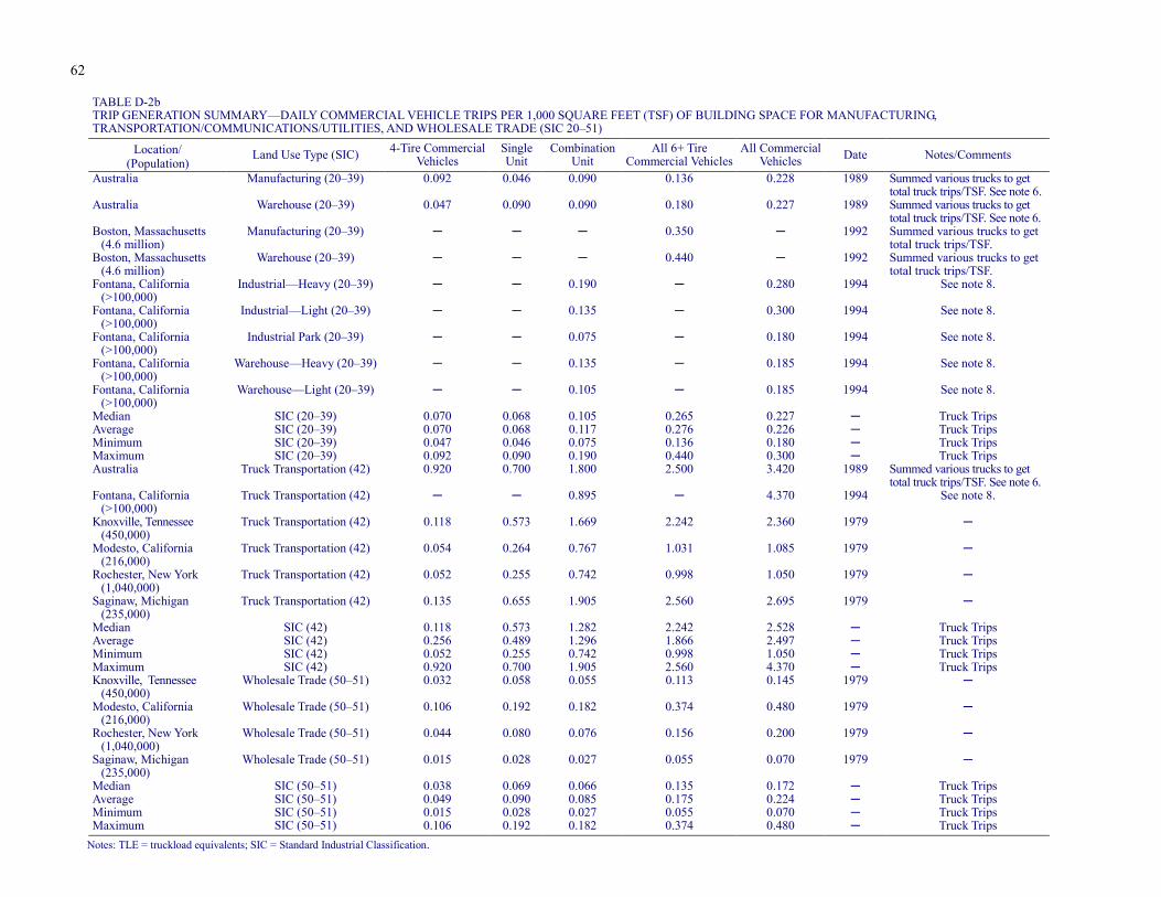
62

TABLE D-2b TRIP GENERATION SUMMARY—DAILY COMMERCIAL VEHICLE TRIPS PER 1,000 SQUARE FEET (TSF) OF BUILDING SPACE FOR MANUFACTURING, TRANSPORTATION/COMMUNICATIONS/UTILITIES, AND WHOLESALE TRADE (SIC 20–51)

Location/ (Population)

Land Use Type (SIC) 4-Tire Commercial Vehicles

Single Unit

Combination Unit

All 6+ Tire Commercial Vehicles

All Commercial Vehicles Date Notes/Comments

Australia Manufacturing (20–39) 0.092 0.046 0.090 0.136 0.228 1989 Summed various trucks to get total truck trips/TSF. See note 6.

Australia Warehouse (20–39) 0.047 0.090 0.090 0.180 0.227 1989 Summed various trucks to get total truck trips/TSF. See note 6.

Boston, Massachusetts (4.6 million)

Manufacturing (20–39) ─ ─ ─ 0.350 ─ 1992 Summed various trucks to get total truck trips/TSF.

Boston, Massachusetts (4.6 million)

Warehouse (20–39) ─ ─ ─ 0.440 ─ 1992 Summed various trucks to get total truck trips/TSF.

Fontana, California (>100,000)

Industrial—Heavy (20–39) ─ ─ 0.190 ─ 0.280 1994 See note 8.

Fontana, California (>100,000)

Industrial—Light (20–39) ─ ─ 0.135 ─ 0.300 1994 See note 8.

Fontana, California (>100,000)

Industrial Park (20–39) ─ ─ 0.075 ─ 0.180 1994 See note 8.

Fontana, California (>100,000)

Warehouse—Heavy (20–39) ─ ─ 0.135 ─ 0.185 1994 See note 8.

Fontana, California (>100,000)

Warehouse—Light (20–39) ─ ─ 0.105 ─ 0.185 1994 See note 8.

Median SIC (20–39) 0.070 0.068 0.105 0.265 0.227 ─ Truck Trips Average SIC (20–39) 0.070 0.068 0.117 0.276 0.226 ─ Truck Trips Minimum SIC (20–39) 0.047 0.046 0.075 0.136 0.180 ─ Truck Trips Maximum SIC (20–39) 0.092 0.090 0.190 0.440 0.300 ─ Truck Trips Australia Truck Transportation (42) 0.920 0.700 1.800 2.500 3.420 1989 Summed various trucks to get

total truck trips/TSF. See note 6. Fontana, California

(>100,000) Truck Transportation (42) ─ ─ 0.895 ─ 4.370 1994 See note 8.

Knoxville, Tennessee (450,000)

Truck Transportation (42) 0.118 0.573 1.669 2.242 2.360 1979 ─

Modesto, California (216,000)

Truck Transportation (42) 0.054 0.264 0.767 1.031 1.085 1979 ─

Rochester, New York (1,040,000)

Truck Transportation (42) 0.052 0.255 0.742 0.998 1.050 1979 ─

Saginaw, Michigan (235,000)

Truck Transportation (42) 0.135 0.655 1.905 2.560 2.695 1979 ─

Median SIC (42) 0.118 0.573 1.282 2.242 2.528 ─ Truck Trips Average SIC (42) 0.256 0.489 1.296 1.866 2.497 ─ Truck Trips Minimum SIC (42) 0.052 0.255 0.742 0.998 1.050 ─ Truck Trips Maximum SIC (42) 0.920 0.700 1.905 2.560 4.370 ─ Truck Trips Knoxville, Tennessee

(450,000) Wholesale Trade (50–51) 0.032 0.058 0.055 0.113 0.145 1979 ─

Modesto, California (216,000)

Wholesale Trade (50–51) 0.106 0.192 0.182 0.374 0.480 1979 ─

Rochester, New York (1,040,000)

Wholesale Trade (50–51) 0.044 0.080 0.076 0.156 0.200 1979 ─

Saginaw, Michigan (235,000)

Wholesale Trade (50–51) 0.015 0.028 0.027 0.055 0.070 1979 ─

Median SIC (50–51) 0.038 0.069 0.066 0.135 0.172 ─ Truck Trips Average SIC (50–51) 0.049 0.090 0.085 0.175 0.224 ─ Truck Trips Minimum SIC (50–51) 0.015 0.028 0.027 0.055 0.070 ─ Truck Trips Maximum SIC (50–51) 0.106 0.192 0.182 0.374 0.480 ─ Truck Trips

Notes: TLE = truckload equivalents; SIC = Standard Industrial Classification.

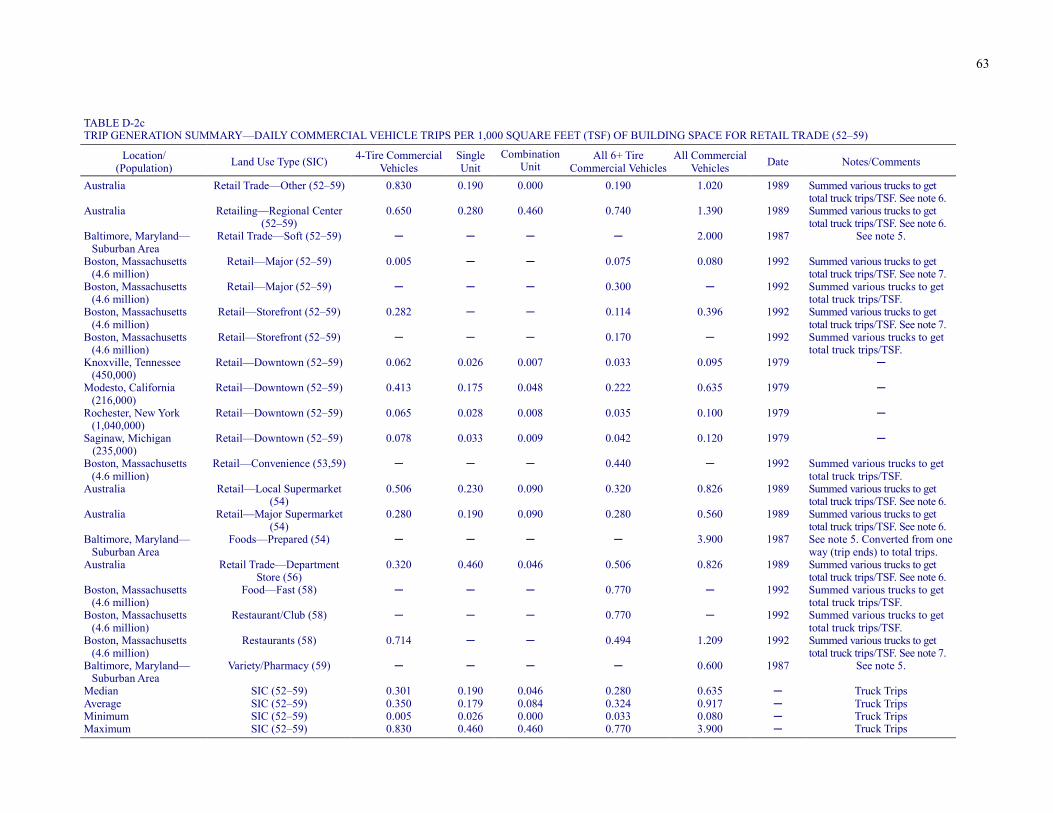
63

TABLE D-2c TRIP GENERATION SUMMARY—DAILY COMMERCIAL VEHICLE TRIPS PER 1,000 SQUARE FEET (TSF) OF BUILDING SPACE FOR RETAIL TRADE (52–59)

Location/ (Population) Land Use Type (SIC) 4-Tire Commercial

Vehicles Single Unit

Combination Unit

All 6+ Tire Commercial Vehicles

All Commercial Vehicles Date Notes/Comments

Australia Retail Trade—Other (52–59) 0.830 0.190 0.000 0.190 1.020 1989 Summed various trucks to get

total truck trips/TSF. See note 6. Australia Retailing—Regional Center

(52–59) 0.650 0.280 0.460 0.740 1.390 1989 Summed various trucks to get

total truck trips/TSF. See note 6. Baltimore, Maryland—

Suburban Area Retail Trade—Soft (52–59) ─ ─ ─ ─ 2.000 1987 See note 5.

Boston, Massachusetts (4.6 million)

Retail—Major (52–59) 0.005 ─ ─ 0.075 0.080 1992 Summed various trucks to get total truck trips/TSF. See note 7.

Boston, Massachusetts (4.6 million)

Retail—Major (52–59) ─ ─ ─ 0.300 ─ 1992 Summed various trucks to get total truck trips/TSF.

Boston, Massachusetts (4.6 million)

Retail—Storefront (52–59) 0.282 ─ ─ 0.114 0.396 1992 Summed various trucks to get total truck trips/TSF. See note 7.

Boston, Massachusetts (4.6 million)

Retail—Storefront (52–59) ─ ─ ─ 0.170 ─ 1992 Summed various trucks to get total truck trips/TSF.

Knoxville, Tennessee (450,000)

Retail—Downtown (52–59) 0.062 0.026 0.007 0.033 0.095 1979 ─

Modesto, California (216,000)

Retail—Downtown (52–59) 0.413 0.175 0.048 0.222 0.635 1979 ─

Rochester, New York (1,040,000)

Retail—Downtown (52–59) 0.065 0.028 0.008 0.035 0.100 1979 ─

Saginaw, Michigan (235,000)

Retail—Downtown (52–59) 0.078 0.033 0.009 0.042 0.120 1979 ─

Boston, Massachusetts (4.6 million)

Retail—Convenience (53,59) ─ ─ ─ 0.440 ─ 1992 Summed various trucks to get total truck trips/TSF.

Australia Retail—Local Supermarket (54)

0.506 0.230 0.090 0.320 0.826 1989 Summed various trucks to get total truck trips/TSF. See note 6.

Australia Retail—Major Supermarket (54)

0.280 0.190 0.090 0.280 0.560 1989 Summed various trucks to get total truck trips/TSF. See note 6.

Baltimore, Maryland—Suburban Area

Foods—Prepared (54) ─ ─ ─ ─ 3.900 1987 See note 5. Converted from one way (trip ends) to total trips.

Australia Retail Trade—Department Store (56)

0.320 0.460 0.046 0.506 0.826 1989 Summed various trucks to get total truck trips/TSF. See note 6.

Boston, Massachusetts (4.6 million)

Food—Fast (58) ─ ─ ─ 0.770 ─ 1992 Summed various trucks to get total truck trips/TSF.

Boston, Massachusetts (4.6 million)

Restaurant/Club (58) ─ ─ ─ 0.770 ─ 1992 Summed various trucks to get total truck trips/TSF.

Boston, Massachusetts (4.6 million)

Restaurants (58) 0.714 ─ ─ 0.494 1.209 1992 Summed various trucks to get total truck trips/TSF. See note 7.

Baltimore, Maryland—Suburban Area

Variety/Pharmacy (59) ─ ─ ─ ─ 0.600 1987 See note 5.

Median SIC (52–59) 0.301 0.190 0.046 0.280 0.635 ─ Truck Trips Average SIC (52–59) 0.350 0.179 0.084 0.324 0.917 ─ Truck Trips Minimum SIC (52–59) 0.005 0.026 0.000 0.033 0.080 ─ Truck Trips Maximum SIC (52–59) 0.830 0.460 0.460 0.770 3.900 ─ Truck Trips

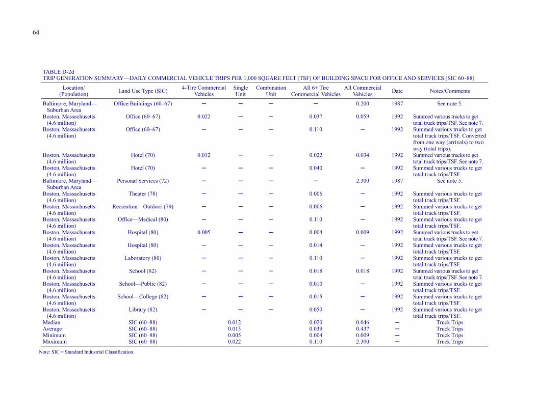
64

TABLE D-2d TRIP GENERATION SUMMARY—DAILY COMMERCIAL VEHICLE TRIPS PER 1,000 SQUARE FEET (TSF) OF BUILDING SPACE FOR OFFICE AND SERVICES (SIC 60–88)

Location/ (Population) Land Use Type (SIC) 4-Tire Commercial

Vehicles Single Unit

Combination Unit

All 6+ Tire Commercial Vehicles

All Commercial Vehicles Date Notes/Comments

Baltimore, Maryland—

Suburban Area Office Buildings (60–67) ─ ─ ─ ─ 0.200 1987 See note 5.

Boston, Massachusetts (4.6 million)

Office (60–67) 0.022 ─ ─ 0.037 0.059 1992 Summed various trucks to get total truck trips/TSF. See note 7.

Boston, Massachusetts (4.6 million)

Office (60–67) ─ ─ ─ 0.110 ─ 1992 Summed various trucks to get total truck trips/TSF. Converted from one way (arrivals) to two way (total trips).

Boston, Massachusetts (4.6 million)

Hotel (70) 0.012 ─ ─ 0.022 0.034 1992 Summed various trucks to get total truck trips/TSF. See note 7.

Boston, Massachusetts (4.6 million)

Hotel (70) ─ ─ ─ 0.040 ─ 1992 Summed various trucks to get total truck trips/TSF.

Baltimore, Maryland—Suburban Area

Personal Services (72) ─ ─ ─ ─ 2.300 1987 See note 5.

Boston, Massachusetts (4.6 million)

Theater (78) ─ ─ ─ 0.006 ─ 1992 Summed various trucks to get total truck trips/TSF.

Boston, Massachusetts (4.6 million)

Recreation—Outdoor (79) ─ ─ ─ 0.006 ─ 1992 Summed various trucks to get total truck trips/TSF.

Boston, Massachusetts (4.6 million)

Office—Medical (80) ─ ─ ─ 0.110 ─ 1992 Summed various trucks to get total truck trips/TSF.

Boston, Massachusetts (4.6 million)

Hospital (80) 0.005 ─ ─ 0.004 0.009 1992 Summed various trucks to get total truck trips/TSF. See note 7.

Boston, Massachusetts (4.6 million)

Hospital (80) ─ ─ ─ 0.014 ─ 1992 Summed various trucks to get total truck trips/TSF.

Boston, Massachusetts (4.6 million)

Laboratory (80) ─ ─ ─ 0.110 ─ 1992 Summed various trucks to get total truck trips/TSF.

Boston, Massachusetts (4.6 million)

School (82) ─ ─ ─ 0.018 0.018 1992 Summed various trucks to get total truck trips/TSF. See note 7.

Boston, Massachusetts (4.6 million)

School—Public (82) ─ ─ ─ 0.010 ─ 1992 Summed various trucks to get total truck trips/TSF.

Boston, Massachusetts (4.6 million)

School—College (82) ─ ─ ─ 0.015 ─ 1992 Summed various trucks to get total truck trips/TSF.

Boston, Massachusetts (4.6 million)

Library (82) ─ ─ ─ 0.050 ─ 1992 Summed various trucks to get total truck trips/TSF.

Median SIC (60–88) 0.012 0.020 0.046 ─ Truck Trips Average SIC (60–88) 0.013 0.039 0.437 ─ Truck Trips Minimum SIC (60–88) 0.005 0.004 0.009 ─ Truck Trips Maximum SIC (60–88) 0.022 0.110 2.300 ─ Truck Trips

Note: SIC = Standard Industrial Classification.

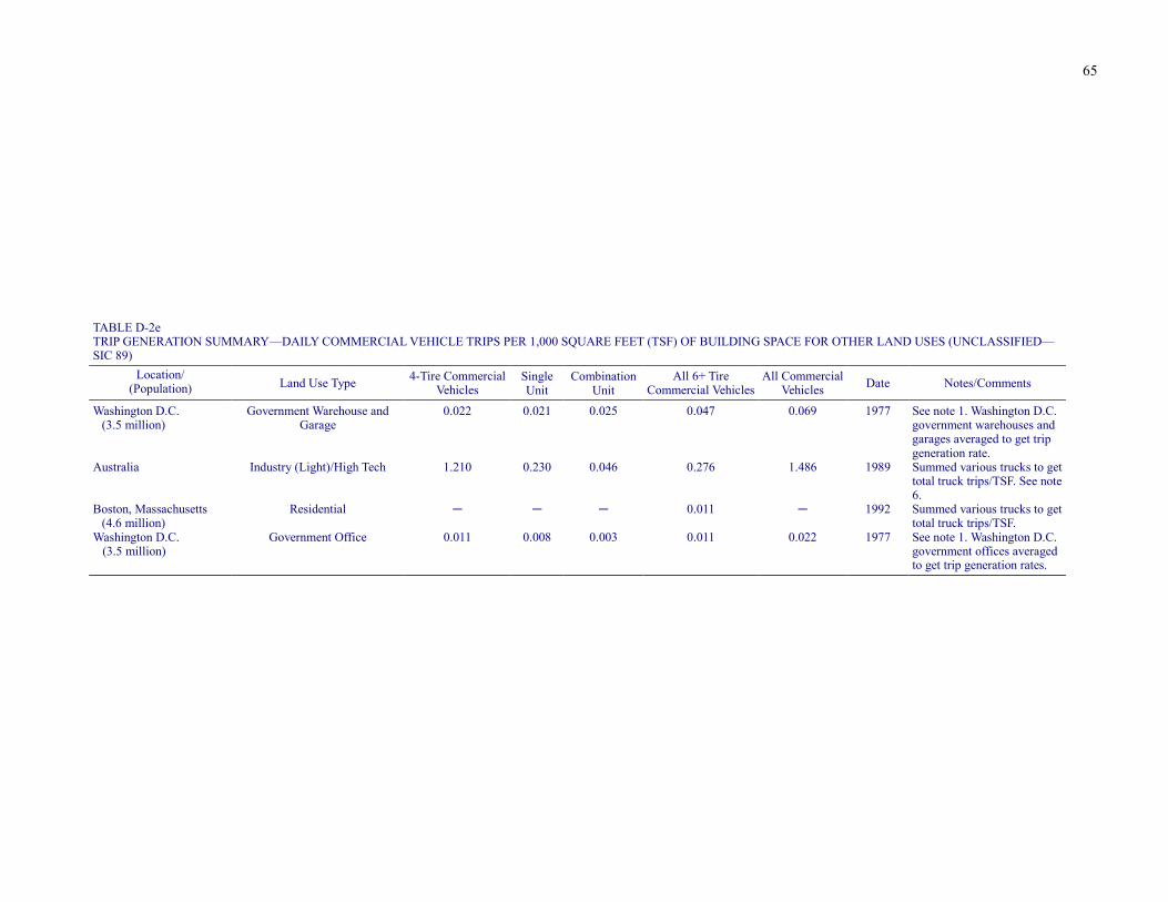
65

TABLE D-2e TRIP GENERATION SUMMARY—DAILY COMMERCIAL VEHICLE TRIPS PER 1,000 SQUARE FEET (TSF) OF BUILDING SPACE FOR OTHER LAND USES (UNCLASSIFIED—SIC 89)

Location/ (Population) Land Use Type 4-Tire Commercial

Vehicles Single Unit

Combination Unit

All 6+ Tire Commercial Vehicles

All Commercial Vehicles Date Notes/Comments

Washington D.C.

(3.5 million) Government Warehouse and

Garage 0.022 0.021 0.025 0.047 0.069 1977 See note 1. Washington D.C.

government warehouses and garages averaged to get trip generation rate.

Australia Industry (Light)/High Tech 1.210 0.230 0.046 0.276 1.486 1989 Summed various trucks to get total truck trips/TSF. See note 6.

Boston, Massachusetts (4.6 million)

Residential ─ ─ ─ 0.011 ─ 1992 Summed various trucks to get total truck trips/TSF.

Washington D.C. (3.5 million)

Government Office 0.011 0.008 0.003 0.011 0.022 1977 See note 1. Washington D.C. government offices averaged to get trip generation rates.

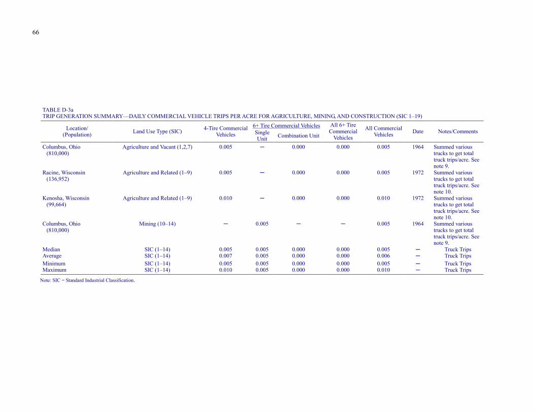
66

TABLE D-3a TRIP GENERATION SUMMARY—DAILY COMMERCIAL VEHICLE TRIPS PER ACRE FOR AGRICULTURE, MINING, AND CONSTRUCTION (SIC 1–19)

6+ Tire Commercial Vehicles Location/ (Population) Land Use Type (SIC) 4-Tire Commercial

Vehicles Single Unit Combination Unit

All 6+ Tire Commercial

Vehicles

All Commercial Vehicles Date Notes/Comments

Columbus, Ohio

(810,000) Agriculture and Vacant (1,2,7) 0.005 ─ 0.000 0.000 0.005 1964 Summed various

trucks to get total truck trips/acre. See note 9.

Racine, Wisconsin (136,952)

Agriculture and Related (1–9) 0.005 ─ 0.000 0.000 0.005 1972 Summed various trucks to get total truck trips/acre. See note 10.

Kenosha, Wisconsin (99,664)

Agriculture and Related (1–9) 0.010 ─ 0.000 0.000 0.010 1972 Summed various trucks to get total truck trips/acre. See note 10.

Columbus, Ohio (810,000)

Mining (10–14) ─ 0.005 ─ ─ 0.005 1964 Summed various trucks to get total truck trips/acre. See note 9.

Median SIC (1–14) 0.005 0.005 0.000 0.000 0.005 ─ Truck Trips Average SIC (1–14) 0.007 0.005 0.000 0.000 0.006 ─ Truck Trips Minimum SIC (1–14) 0.005 0.005 0.000 0.000 0.005 ─ Truck Trips Maximum SIC (1–14) 0.010 0.005 0.000 0.000 0.010 ─ Truck Trips

Note: SIC = Standard Industrial Classification.

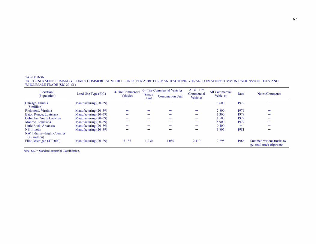
67

TABLE D-3b TRIP GENERATION SUMMARY—DAILY COMMERCIAL VEHICLE TRIPS PER ACRE FOR MANUFACTURING, TRANSPORTATION/COMMUNICATIONS/UTILITIES, AND WHOLESALE TRADE (SIC 20–51)

6+ Tire Commercial Vehicles Location/ (Population) Land Use Type (SIC) 4-Tire Commercial

Vehicles Single Unit Combination Unit

All 6+ Tire Commercial

Vehicles

All Commercial Vehicles Date Notes/Comments

Chicago, Illinois (8 million)

Manufacturing (20–39) ─ ─ ─ ─ 3.600 1979 ─

Richmond, Virginia Manufacturing (20–39) ─ ─ ─ ─ 2.800 1979 ─ Baton Rouge, Louisiana Manufacturing (20–39) ─ ─ ─ ─ 1.300 1979 ─ Columbia, South Carolina Manufacturing (20–39) ─ ─ ─ ─ 1.500 1979 ─ Monroe, Louisiana Manufacturing (20–39) ─ ─ ─ ─ 5.900 1979 ─ Little Rock, Arkansas Manufacturing (20–39) ─ ─ ─ ─ 0.400 ─ ─ NE Illinois/ NW Indiana—Eight Counties

(>8 million)

Manufacturing (20–39) ─ ─ ─ ─ 1.805 1981 ─

Flint, Michigan (470,000) Manufacturing (20–39) 5.185 1.030 1.080 2.110 7.295 1966 Summed various trucks to get total truck trips/acre.

Note: SIC = Standard Industrial Classification.

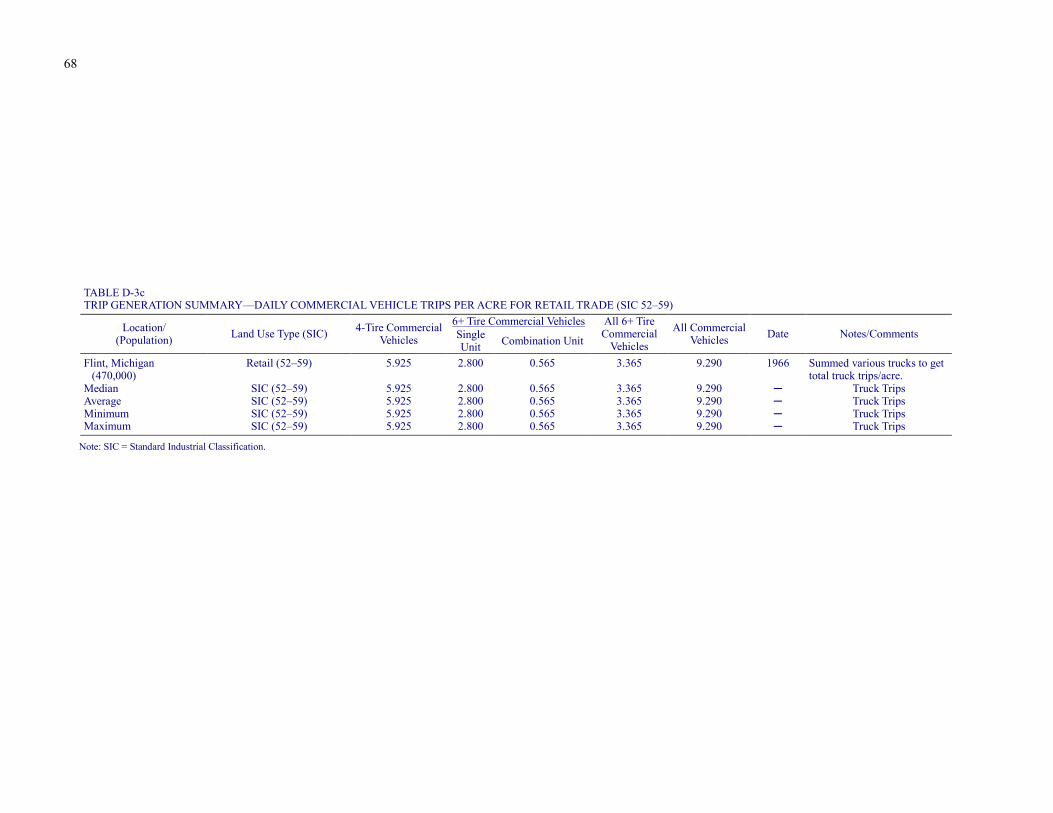
68

TABLE D-3c TRIP GENERATION SUMMARY—DAILY COMMERCIAL VEHICLE TRIPS PER ACRE FOR RETAIL TRADE (SIC 52–59)

6+ Tire Commercial VehiclesLocation/ (Population) Land Use Type (SIC) 4-Tire Commercial

Vehicles Single Unit Combination Unit

All 6+ Tire Commercial

Vehicles

All Commercial Vehicles Date Notes/Comments

Flint, Michigan

(470,000) Retail (52–59) 5.925 2.800 0.565 3.365 9.290 1966 Summed various trucks to get

total truck trips/acre. Median SIC (52–59) 5.925 2.800 0.565 3.365 9.290 ─ Truck Trips Average SIC (52–59) 5.925 2.800 0.565 3.365 9.290 ─ Truck Trips Minimum SIC (52–59) 5.925 2.800 0.565 3.365 9.290 ─ Truck Trips Maximum SIC (52–59) 5.925 2.800 0.565 3.365 9.290 ─ Truck Trips

Note: SIC = Standard Industrial Classification.

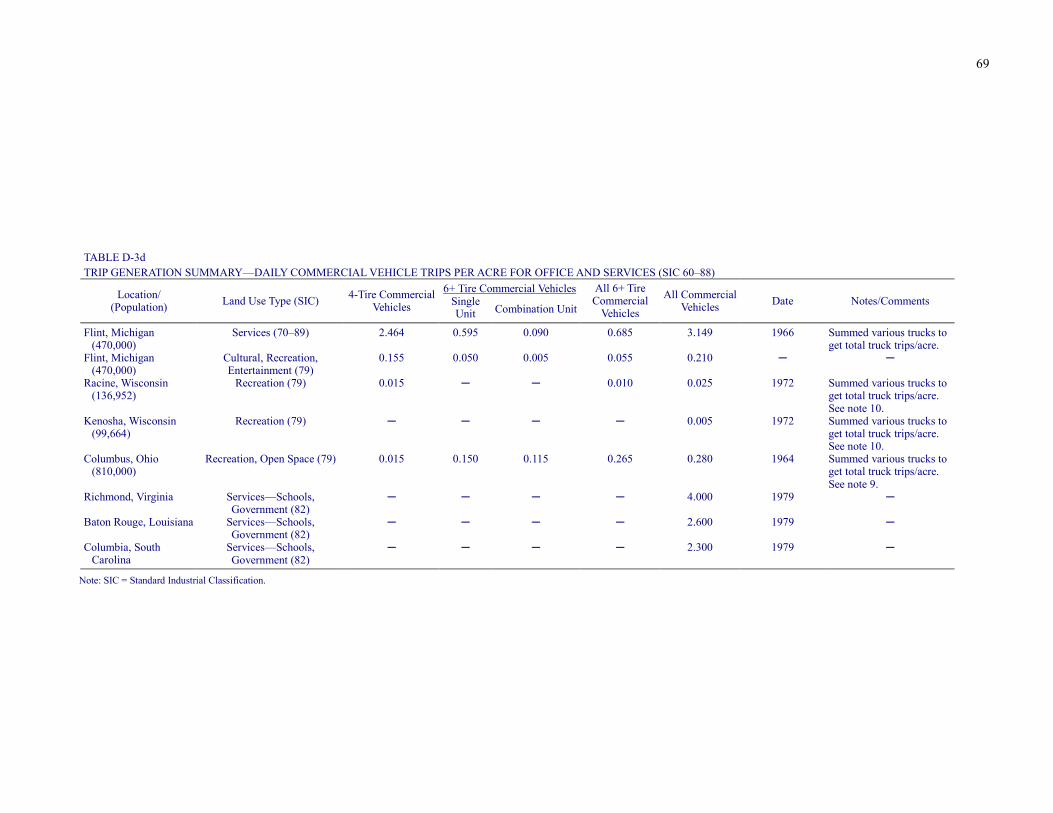
69

TABLE D-3d TRIP GENERATION SUMMARY—DAILY COMMERCIAL VEHICLE TRIPS PER ACRE FOR OFFICE AND SERVICES (SIC 60–88)

6+ Tire Commercial VehiclesLocation/ (Population) Land Use Type (SIC) 4-Tire Commercial

Vehicles Single Unit Combination Unit

All 6+ Tire Commercial

Vehicles

All Commercial Vehicles Date Notes/Comments

Flint, Michigan

(470,000) Services (70–89) 2.464 0.595 0.090 0.685 3.149 1966 Summed various trucks to

get total truck trips/acre. Flint, Michigan

(470,000) Cultural, Recreation, Entertainment (79)

0.155 0.050 0.005 0.055 0.210 ─ ─

Racine, Wisconsin (136,952)

Recreation (79) 0.015 ─ ─ 0.010 0.025 1972 Summed various trucks to get total truck trips/acre. See note 10.

Kenosha, Wisconsin (99,664)

Recreation (79) ─ ─ ─ ─ 0.005 1972 Summed various trucks to get total truck trips/acre. See note 10.

Columbus, Ohio (810,000)

Recreation, Open Space (79) 0.015 0.150 0.115 0.265 0.280 1964 Summed various trucks to get total truck trips/acre. See note 9.

Richmond, Virginia Services—Schools, Government (82)

─ ─ ─ ─ 4.000 1979 ─

Baton Rouge, Louisiana Services—Schools, Government (82)

─ ─ ─ ─ 2.600 1979 ─

Columbia, South Carolina

Services—Schools, Government (82)

─ ─ ─ ─ 2.300 1979 ─

Note: SIC = Standard Industrial Classification.

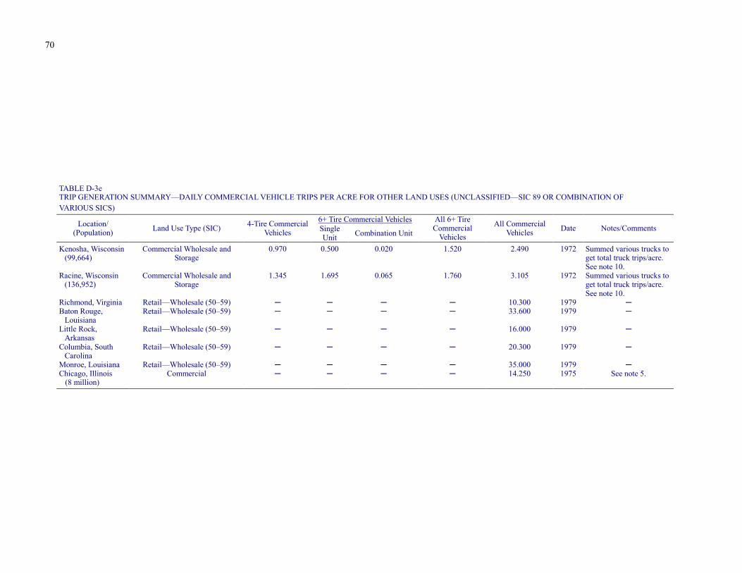
70

TABLE D-3e TRIP GENERATION SUMMARY—DAILY COMMERCIAL VEHICLE TRIPS PER ACRE FOR OTHER LAND USES (UNCLASSIFIED—SIC 89 OR COMBINATION OF VARIOUS SICS)

6+ Tire Commercial Vehicles Location/ (Population) Land Use Type (SIC) 4-Tire Commercial

Vehicles Single Unit Combination Unit

All 6+ Tire Commercial

Vehicles

All Commercial Vehicles Date Notes/Comments

Kenosha, Wisconsin

(99,664) Commercial Wholesale and

Storage 0.970 0.500 0.020 1.520 2.490 1972 Summed various trucks to

get total truck trips/acre. See note 10.

Racine, Wisconsin (136,952)

Commercial Wholesale and Storage

1.345 1.695 0.065 1.760 3.105 1972 Summed various trucks to get total truck trips/acre. See note 10.

Richmond, Virginia Retail––Wholesale (50–59) ─ ─ ─ ─ 10.300 1979 ─ Baton Rouge,

Louisiana Retail––Wholesale (50–59) ─ ─ ─ ─ 33.600 1979 ─

Little Rock, Arkansas

Retail––Wholesale (50–59) ─ ─ ─ ─ 16.000 1979 ─

Columbia, South Carolina

Retail––Wholesale (50–59) ─ ─ ─ ─ 20.300 1979 ─

Monroe, Louisiana Retail––Wholesale (50–59) ─ ─ ─ ─ 35.000 1979 ─ Chicago, Illinois (8 million)

Commercial ─ ─ ─ ─ 14.250 1975 See note 5.

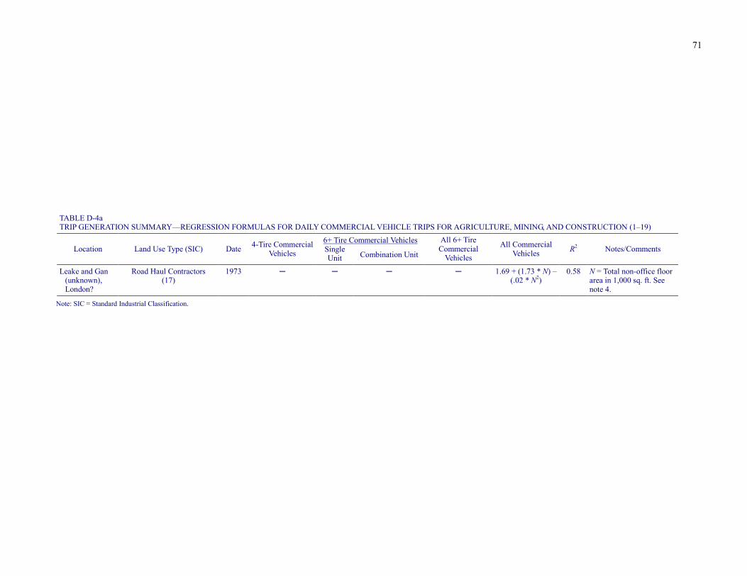
71

TABLE D-4a TRIP GENERATION SUMMARY—REGRESSION FORMULAS FOR DAILY COMMERCIAL VEHICLE TRIPS FOR AGRICULTURE, MINING, AND CONSTRUCTION (1–19)

6+ Tire Commercial Vehicles Location Land Use Type (SIC) Date 4-Tire Commercial

Vehicles Single Unit Combination Unit

All 6+ Tire Commercial

Vehicles

All Commercial Vehicles R2 Notes/Comments

Leake and Gan

(unknown), London?

Road Haul Contractors (17)

1973 ─ ─ ─ ─ 1.69 + (1.73 * N) – (.02 * N2)

0.58 N = Total non-office floor area in 1,000 sq. ft. See note 4.

Note: SIC = Standard Industrial Classification.

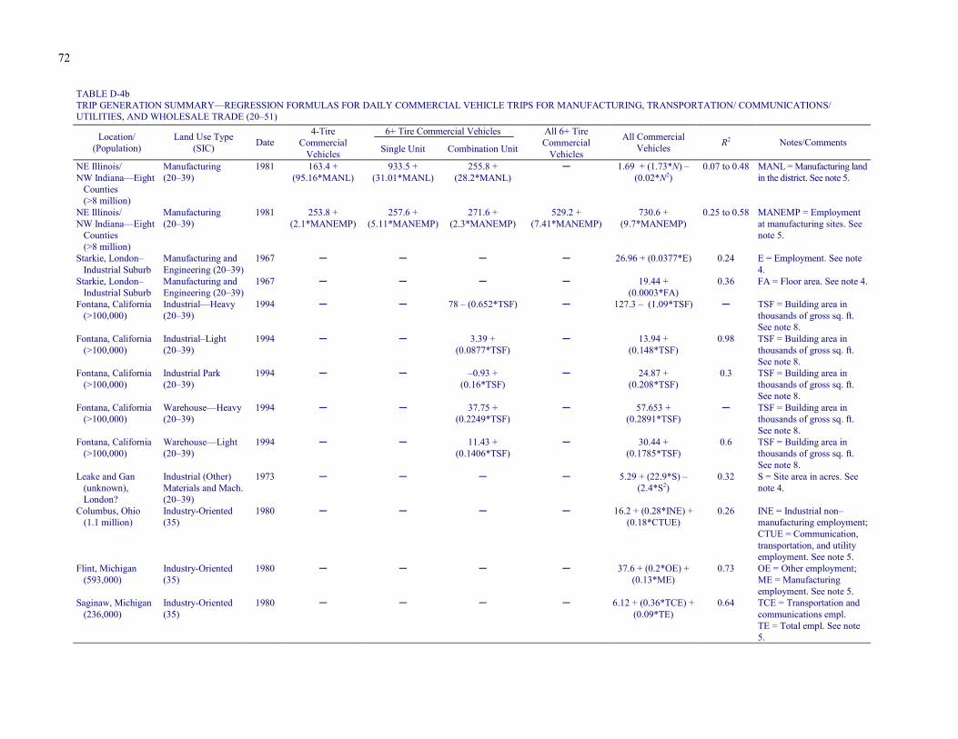
72

TABLE D-4b TRIP GENERATION SUMMARY—REGRESSION FORMULAS FOR DAILY COMMERCIAL VEHICLE TRIPS FOR MANUFACTURING, TRANSPORTATION/ COMMUNICATIONS/ UTILITIES, AND WHOLESALE TRADE (20–51)

6+ Tire Commercial Vehicles Location/ (Population)

Land Use Type (SIC) Date

4-Tire Commercial

Vehicles Single Unit Combination Unit

All 6+ Tire Commercial

Vehicles

All Commercial Vehicles R2 Notes/Comments

NE Illinois/ NW Indiana—Eight

Counties (>8 million)

Manufacturing (20–39)

1981 163.4 + (95.16*MANL)

933.5 + (31.01*MANL)

255.8 + (28.2*MANL)

─ 1.69 + (1.73*N) – (0.02*N2)

0.07 to 0.48 MANL = Manufacturing land in the district. See note 5.

NE Illinois/ NW Indiana—Eight

Counties (>8 million)

Manufacturing (20–39)

1981 253.8 + (2.1*MANEMP)

257.6 + (5.11*MANEMP)

271.6 + (2.3*MANEMP)

529.2 + (7.41*MANEMP)

730.6 + (9.7*MANEMP)

0.25 to 0.58 MANEMP = Employment at manufacturing sites. See note 5.

Starkie, London–Industrial Suburb

Manufacturing and Engineering (20–39)

1967 ─ ─ ─ ─ 26.96 + (0.0377*E) 0.24 E = Employment. See note 4.

Starkie, London–Industrial Suburb

Manufacturing and Engineering (20–39)

1967 ─ ─ ─ ─ 19.44 + (0.0003*FA)

0.36 FA = Floor area. See note 4.

Fontana, California (>100,000)

Industrial—Heavy (20–39)

1994 ─ ─ 78 – (0.652*TSF) ─ 127.3 – (1.09*TSF) ─ TSF = Building area in thousands of gross sq. ft. See note 8.

Fontana, California (>100,000)

Industrial–Light (20–39)

1994 ─ ─ 3.39 + (0.0877*TSF)

─ 13.94 + (0.148*TSF)

0.98 TSF = Building area in thousands of gross sq. ft. See note 8.

Fontana, California (>100,000)

Industrial Park (20–39)

1994 ─ ─ –0.93 + (0.16*TSF)

─ 24.87 + (0.208*TSF)

0.3 TSF = Building area in thousands of gross sq. ft. See note 8.

Fontana, California (>100,000)

Warehouse—Heavy (20–39)

1994 ─ ─ 37.75 + (0.2249*TSF)

─ 57.653 + (0.2891*TSF)

─ TSF = Building area in thousands of gross sq. ft. See note 8.

Fontana, California (>100,000)

Warehouse—Light (20–39)

1994 ─ ─ 11.43 + (0.1406*TSF)

─ 30.44 + (0.1785*TSF)

0.6 TSF = Building area in thousands of gross sq. ft. See note 8.

Leake and Gan (unknown), London?

Industrial (Other) Materials and Mach. (20–39)

1973 ─ ─ ─ ─ 5.29 + (22.9*S) –(2.4*S2)

0.32 S = Site area in acres. See note 4.

Columbus, Ohio (1.1 million)

Industry-Oriented (35)

1980 ─ ─ ─ ─ 16.2 + (0.28*INE) + (0.18*CTUE)

0.26 INE = Industrial non–manufacturing employment; CTUE = Communication, transportation, and utility employment. See note 5.

Flint, Michigan (593,000)

Industry-Oriented (35)

1980 ─ ─ ─ ─ 37.6 + (0.2*OE) + (0.13*ME)

0.73 OE = Other employment; ME = Manufacturing employment. See note 5.

Saginaw, Michigan (236,000)

Industry-Oriented (35)

1980 ─ ─ ─ ─ 6.12 + (0.36*TCE) + (0.09*TE)

0.64 TCE = Transportation and communications empl. TE = Total empl. See note 5.

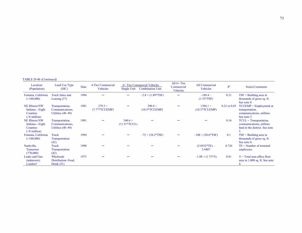
73

TABLE D-4b (Continued)

Location/ (Population)

Land Use Type (SIC) Date 4-Tire Commercial

Vehicles 6+ Tire Commercial Vehicles

Single Unit Combination Unit

All 6+ Tire Commercial

Vehicles

All Commercial Vehicles R2 Notes/Comments

Fontana, California

(>100,000) Truck Sales and Leasing (37)

1994 ─ ─ –2.8 + (1.89*TSF) ─ –189.4 – (1.53*TSF)

0.21 TSF = Building area in thousands of gross sq. ft. See note 8.

NE Illinois/NW Indiana—Eight Counties (>8 million)

Transportation, Communications, Utilities (40–49)

1981 279.3 + (7.77*TCUEMP)

─ 390.4 + (10.5*TCUEMP)

─ 1384.1 + (10.3*TCUEMP)

0.21 to 0.65 TCUEMP = Employment at transportation, communications, utilities. See note 5.

NE Illinois/NW Indiana—Eight Counties (>8 million)

Transportation, Communications, Utilities (40–49)

1981 ─ 540.6 + (11.51*TCUL)

─ ─ ─ 0.16 TCUL = Transportation, communications, utilities land in the district. See note 5.

Fontana, California (>100,000)

Truck Transportation (42)

1994 ─ ─ –72 + (38.2*TSF) ─ –108 + (50.6*TSF) 0.1 TSF = Building area in thousands of gross sq. ft. See note 8.

Nashville, Tennessee (770,000)

Truck Transportation (42)

1990 ─ ─ ─ ─ (2.0552*TE) – 3.4407

0.726 TE = Number of terminal employees.

Leake and Gan (unknown), London?

Wholesale Distribution–Food, Drink (51)

1973 ─ ─ ─ ─ –1.88 + (1.75*N) 0.81 N = Total non-office floor area in 1,000 sq. ft. See note 4.

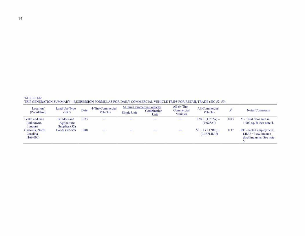
74

TABLE D-4c TRIP GENERATION SUMMARY—REGRESSION FORMULAS FOR DAILY COMMERCIAL VEHICLE TRIPS FOR RETAIL TRADE (SIC 52–59)

6+ Tire Commercial Vehicles Location/ (Population)

Land Use Type (SIC) Date 4-Tire Commercial

Vehicles Single Unit Combination Unit

All 6+ Tire Commercial

Vehicles

All Commercial Vehicles R2 Notes/Comments

Leake and Gan

(unknown), London?

Builders and Agriculture

Supplies (52)

1973 ─ ─ ─ ─ 1.69 + (1.73*N) – (0.02*N2)

0.83 F = Total floor area in 1,000 sq. ft. See note 4.

Gastonia, North Carolina (166,000)

Goods (52–59) 1980 ─ ─ ─ ─ 50.1 + (1.1*RE) + (0.33*LIDU)

0.37 RE = Retail employment; LIDU = Low-income dwelling units. See note 5.

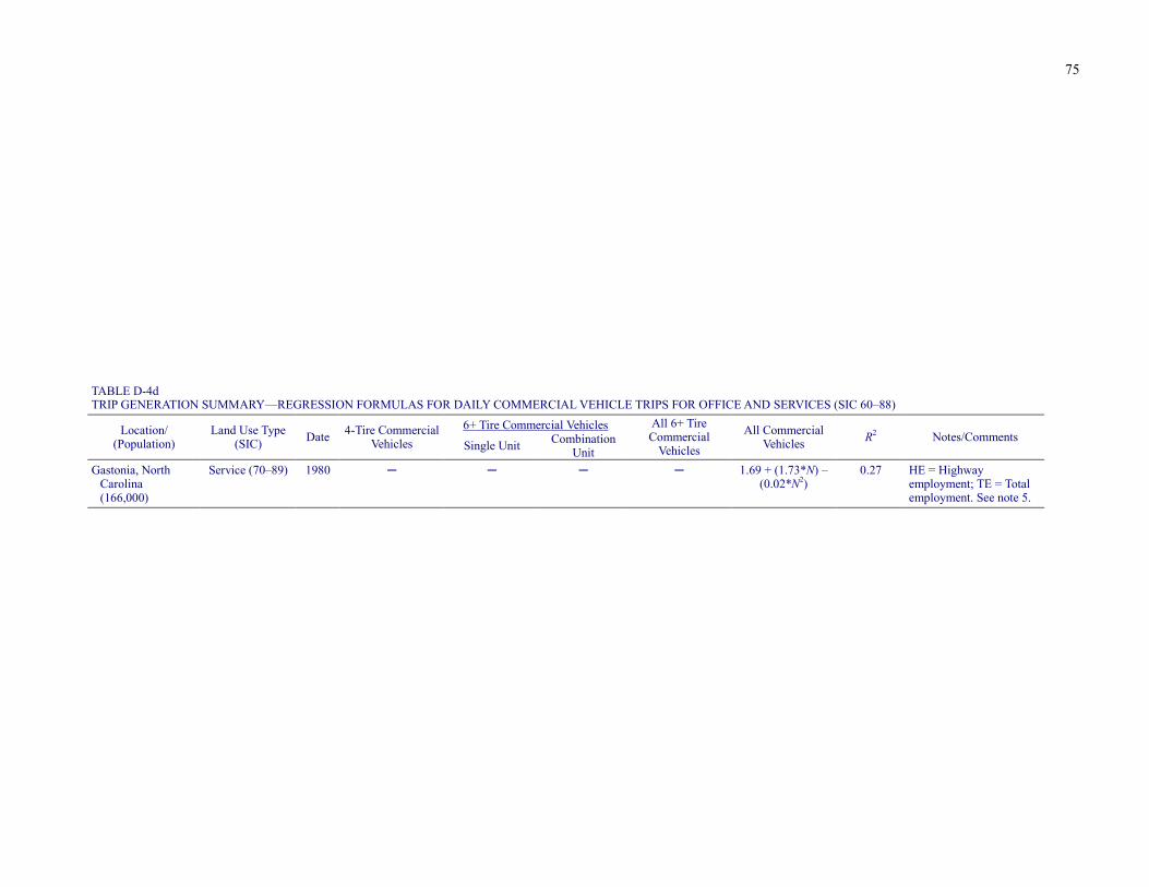
75

TABLE D-4d TRIP GENERATION SUMMARY—REGRESSION FORMULAS FOR DAILY COMMERCIAL VEHICLE TRIPS FOR OFFICE AND SERVICES (SIC 60–88)

6+ Tire Commercial Vehicles Location/ (Population)

Land Use Type (SIC) Date 4-Tire Commercial

Vehicles Single Unit Combination Unit

All 6+ Tire Commercial

Vehicles

All Commercial Vehicles R2 Notes/Comments

Gastonia, North

Carolina (166,000)

Service (70–89) 1980 ─ ─ ─ ─ 1.69 + (1.73*N) – (0.02*N2)

0.27 HE = Highway employment; TE = Total employment. See note 5.

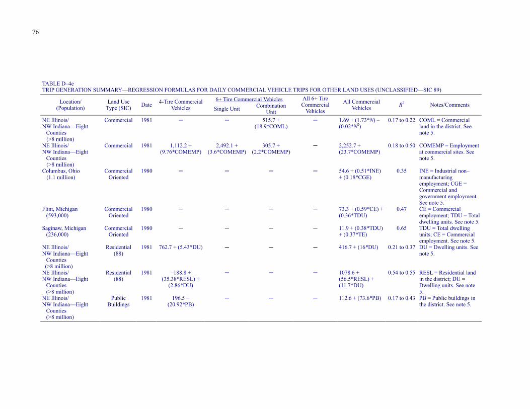
76

TABLE D–4e TRIP GENERATION SUMMARY—REGRESSION FORMULAS FOR DAILY COMMERCIAL VEHICLE TRIPS FOR OTHER LAND USES (UNCLASSIFIED—SIC 89)

6+ Tire Commercial Vehicles Location/ (Population)

Land Use Type (SIC) Date 4-Tire Commercial

Vehicles Single Unit Combination Unit

All 6+ Tire Commercial

Vehicles

All Commercial Vehicles R2 Notes/Comments

NE Illinois/ NW Indiana—Eight

Counties (>8 million)

Commercial 1981 ─ ─ 515.7 + (18.9*COML)

─ 1.69 + (1.73*N) – (0.02*N2)

0.17 to 0.22 COML = Commercial land in the district. See note 5.

NE Illinois/ NW Indiana—Eight

Counties (>8 million)

Commercial 1981 1,112.2 + (9.76*COMEMP)

2,492.1 + (3.6*COMEMP)

305.7 + (2.2*COMEMP)

─ 2,252.7 + (23.7*COMEMP)

0.18 to 0.50 COMEMP = Employment at commercial sites. See note 5.

Columbus, Ohio (1.1 million)

Commercial Oriented

1980 ─ ─ ─ ─ 54.6 + (0.51*INE) + (0.18*CGE)

0.35 INE = Industrial non–manufacturing employment; CGE = Commercial and government employment. See note 5.

Flint, Michigan (593,000)

Commercial Oriented

1980 ─ ─ ─ ─ 73.3 + (0.59*CE) + (0.36*TDU)

0.47 CE = Commercial employment; TDU = Total dwelling units. See note 5.

Saginaw, Michigan (236,000)

Commercial Oriented

1980 ─ ─ ─ ─ 11.9 + (0.38*TDU) + (0.37*TE)

0.65 TDU = Total dwelling units; CE = Commercial employment. See note 5.

NE Illinois/ NW Indiana—Eight

Counties (>8 million)

Residential (88)

1981 762.7 + (5.43*DU) ─ ─ ─ 416.7 + (16*DU) 0.21 to 0.37 DU = Dwelling units. See note 5.

NE Illinois/ NW Indiana—Eight

Counties (>8 million)

Residential (88)

1981 –188.8 + (35.38*RESL) +

(2.86*DU)

─ ─ ─ 1078.6 + (56.5*RESL) + (11.7*DU)

0.54 to 0.55 RESL = Residential land in the district; DU = Dwelling units. See note 5.

NE Illinois/ NW Indiana—Eight

Counties (>8 million)

Public Buildings

1981 196.5 + (20.92*PB)

─ ─ ─ 112.6 + (73.6*PB) 0.17 to 0.43 PB = Public buildings in the district. See note 5.

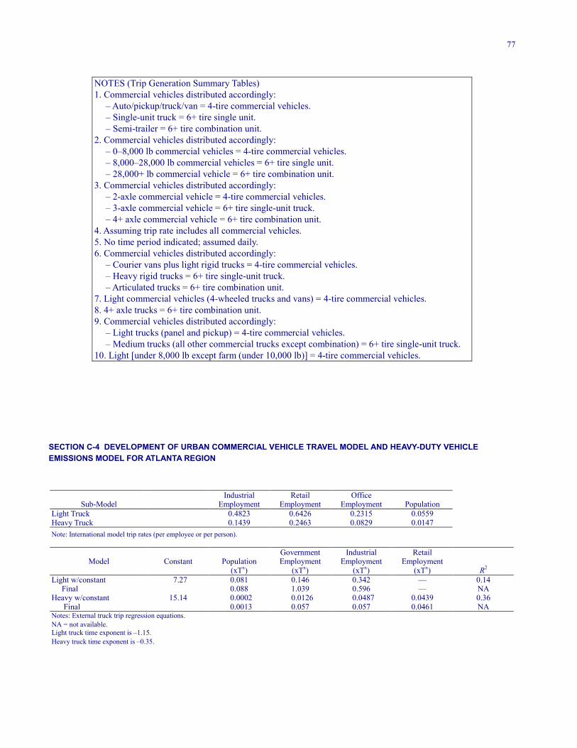
77

NOTES (Trip Generation Summary Tables) 1. Commercial vehicles distributed accordingly:

– Auto/pickup/truck/van = 4-tire commercial vehicles. – Single-unit truck = 6+ tire single unit. – Semi-trailer = 6+ tire combination unit.

2. Commercial vehicles distributed accordingly: – 0–8,000 lb commercial vehicles = 4-tire commercial vehicles. – 8,000–28,000 lb commercial vehicles = 6+ tire single unit. – 28,000+ lb commercial vehicle = 6+ tire combination unit.

3. Commercial vehicles distributed accordingly: – 2-axle commercial vehicle = 4-tire commercial vehicles. – 3-axle commercial vehicle = 6+ tire single-unit truck. – 4+ axle commercial vehicle = 6+ tire combination unit.

4. Assuming trip rate includes all commercial vehicles. 5. No time period indicated; assumed daily. 6. Commercial vehicles distributed accordingly:

– Courier vans plus light rigid trucks = 4-tire commercial vehicles. – Heavy rigid trucks = 6+ tire single-unit truck. – Articulated trucks = 6+ tire combination unit.

7. Light commercial vehicles (4-wheeled trucks and vans) = 4-tire commercial vehicles. 8. 4+ axle trucks = 6+ tire combination unit. 9. Commercial vehicles distributed accordingly:

– Light trucks (panel and pickup) = 4-tire commercial vehicles. – Medium trucks (all other commercial trucks except combination) = 6+ tire single-unit truck.

10. Light [under 8,000 lb except farm (under 10,000 lb)] = 4-tire commercial vehicles. SECTION C-4 DEVELOPMENT OF URBAN COMMERCIAL VEHICLE TRAVEL MODEL AND HEAVY-DUTY VEHICLE EMISSIONS MODEL FOR ATLANTA REGION

Sub-Model

Industrial Employment

Retail Employment

Office Employment

Population

Light Truck 0.4823 0.6426 0.2315 0.0559 Heavy Truck 0.1439 0.2463 0.0829 0.0147 Note: International model trip rates (per employee or per person).

Model

Constant

Population

Government Employment

Industrial Employment

Retail Employment

(xTx) (xTx) (xTx) (xTx) R2

Light w/constant 7.27 0.081 0.146 0.342 — 0.14 Final 0.088 1.039 0.596 — NA Heavy w/constant 15.14 0.0002 0.0126 0.0487 0.0439 0.36 Final 0.0013 0.057 0.057 0.0461 NA Notes: External truck trip regression equations. NA = not available. Light truck time exponent is –1.15. Heavy truck time exponent is –0.35.

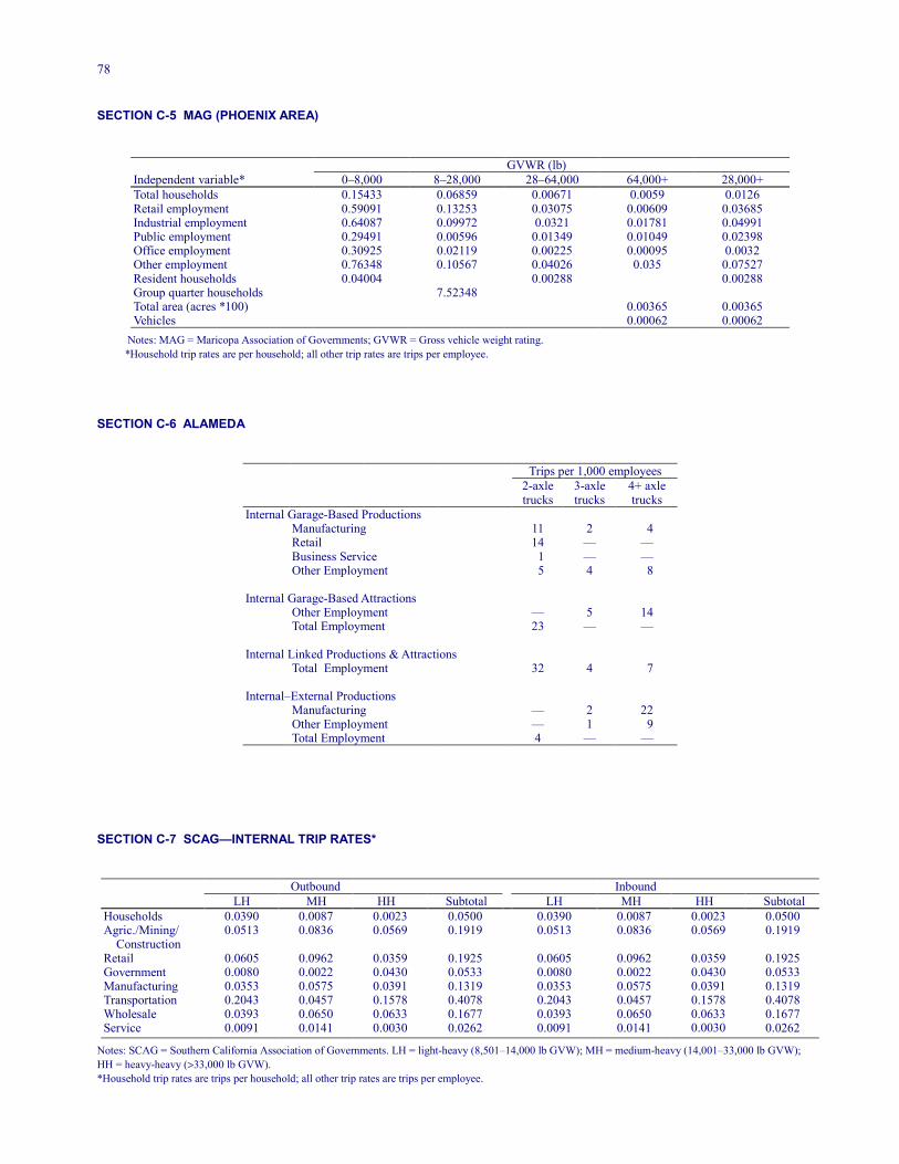
78

SECTION C-5 MAG (PHOENIX AREA)

GVWR (lb) Independent variable* 0–8,000 8–28,000 28–64,000 64,000+ 28,000+ Total households 0.15433 0.06859 0.00671 0.0059 0.0126 Retail employment 0.59091 0.13253 0.03075 0.00609 0.03685 Industrial employment 0.64087 0.09972 0.0321 0.01781 0.04991 Public employment 0.29491 0.00596 0.01349 0.01049 0.02398 Office employment 0.30925 0.02119 0.00225 0.00095 0.0032 Other employment 0.76348 0.10567 0.04026 0.035 0.07527 Resident households 0.04004 0.00288 0.00288 Group quarter households 7.52348 Total area (acres *100) 0.00365 0.00365 Vehicles 0.00062 0.00062

Notes: MAG = Maricopa Association of Governments; GVWR = Gross vehicle weight rating. *Household trip rates are per household; all other trip rates are trips per employee.

SECTION C-6 ALAMEDA

Trips per 1,000 employees 2-axle 3-axle 4+ axle trucks trucks trucks Internal Garage-Based Productions Manufacturing 11 2 4 Retail 14 — — Business Service 1 — — Other Employment 5 4 8 Internal Garage-Based Attractions Other Employment — 5 14 Total Employment 23 — — Internal Linked Productions & Attractions Total Employment 32 4 7 Internal–External Productions Manufacturing — 2 22 Other Employment — 1 9 Total Employment 4 — —

SECTION C-7 SCAG—INTERNAL TRIP RATES*

Outbound Inbound LH MH HH Subtotal LH MH HH Subtotal Households 0.0390 0.0087 0.0023 0.0500 0.0390 0.0087 0.0023 0.0500 Agric./Mining/ Construction

0.0513 0.0836 0.0569 0.1919 0.0513 0.0836 0.0569 0.1919

Retail 0.0605 0.0962 0.0359 0.1925 0.0605 0.0962 0.0359 0.1925 Government 0.0080 0.0022 0.0430 0.0533 0.0080 0.0022 0.0430 0.0533 Manufacturing 0.0353 0.0575 0.0391 0.1319 0.0353 0.0575 0.0391 0.1319 Transportation 0.2043 0.0457 0.1578 0.4078 0.2043 0.0457 0.1578 0.4078 Wholesale 0.0393 0.0650 0.0633 0.1677 0.0393 0.0650 0.0633 0.1677 Service 0.0091 0.0141 0.0030 0.0262 0.0091 0.0141 0.0030 0.0262

Notes: SCAG = Southern California Association of Governments. LH = light-heavy (8,501–14,000 lb GVW); MH = medium-heavy (14,001–33,000 lb GVW); HH = heavy-heavy (>33,000 lb GVW). *Household trip rates are trips per household; all other trip rates are trips per employee.

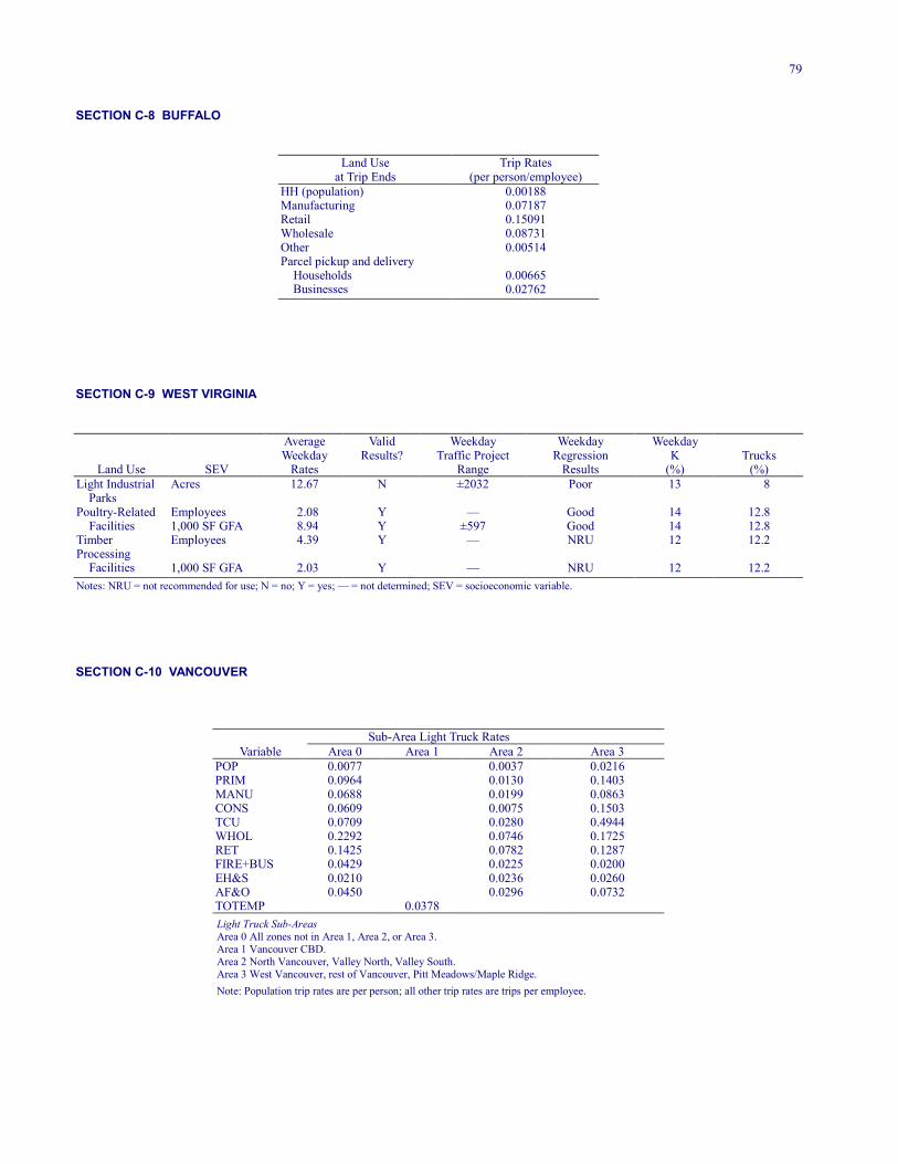
79

SECTION C-8 BUFFALO

Land Use Trip Rates at Trip Ends (per person/employee)

HH (population) 0.00188 Manufacturing 0.07187 Retail 0.15091 Wholesale 0.08731 Other 0.00514 Parcel pickup and delivery Households Businesses

0.00665 0.02762

SECTION C-9 WEST VIRGINIA

Average Valid Weekday Weekday Weekday

Land Use

SEV Weekday

Rates Results? Traffic Project

Range Regression

Results K

(%) Trucks

(%) Light Industrial Parks

Acres 12.67 N ±2032 Poor 13 8

Poultry-Related Employees 2.08 Y — Good 14 12.8 Facilities 1,000 SF GFA 8.94 Y ±597 Good 14 12.8 Timber Processing

Employees 4.39 Y — NRU 12 12.2

Facilities 1,000 SF GFA 2.03 Y — NRU 12 12.2 Notes: NRU = not recommended for use; N = no; Y = yes; — = not determined; SEV = socioeconomic variable. SECTION C-10 VANCOUVER

Sub-Area Light Truck Rates Variable Area 0 Area 1 Area 2 Area 3

POP 0.0077 0.0037 0.0216 PRIM 0.0964 0.0130 0.1403 MANU 0.0688 0.0199 0.0863 CONS 0.0609 0.0075 0.1503 TCU 0.0709 0.0280 0.4944 WHOL 0.2292 0.0746 0.1725 RET 0.1425 0.0782 0.1287 FIRE+BUS 0.0429 0.0225 0.0200 EH&S 0.0210 0.0236 0.0260 AF&O 0.0450 0.0296 0.0732 TOTEMP 0.0378 Light Truck Sub-Areas Area 0 All zones not in Area 1, Area 2, or Area 3. Area 1 Vancouver CBD. Area 2 North Vancouver, Valley North, Valley South. Area 3 West Vancouver, rest of Vancouver, Pitt Meadows/Maple Ridge. Note: Population trip rates are per person; all other trip rates are trips per employee.

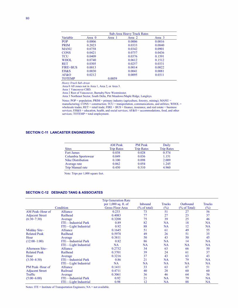
80

Sub-Area Heavy Truck Rates Variable Area 0 Area 1 Area 2 Area 3 POP 0.0006 0.0006 0.0016 PRIM 0.2023 0.0333 0.0840 MANU 0.0758 0.0342 0.0901 CONS 0.0421 0.0757 0.0436 TCU 0.0409 0.0376 0.1591 WHOL 0.0740 0.0612 0.1512 RET 0.0305 0.0257 0.0331 FIRE+BUS 0.0013 0.0014 0.0022 EH&S 0.0030 0.0041 0.0081 AF&O 0.0212 0.0095 0.0311 TOTEMP 0.0059 Heavy Truck Sub-Areas Area 0 All zones not in Area 1, Area 2, or Area 3. Area 1 Vancouver CBD. Area 2 Rest of Vancouver, Burnaby/New Westminster. Area 3 Northeast Sector, South Delta, Pitt Meadows/Maple Ridge, Langleys. Notes: POP = population; PRIM = primary industry (agriculture, forestry, mining); MANU = manufacturing; CONS = construction; TCU = transportation, communications, and utilities; WHOL = wholesale trades; RET = retail trade; FIRE + BUS = finance, insurance, and real estate + business services; EH&S = education, health, and social services; AF&O = accommodations, food, and other services; TOTEMP = total employment.

SECTION C-11 LANCASTER ENGINEERING

AM Peak PM Peak Daily Sites Trip Rates Trip Rates Trip Rates Fort James 0.038 0.028 0.574 Columbia Sportswear 0.049 0.036 1.151 Nike Distribution 0.100 0.098 2.009 Average rate 0.062 0.054 1.245 Trip Manual rate 0.450 0.510 4.960

Note: Trips per 1,000 square feet. SECTION C-12 DESHAZO TANG & ASSOCIATES Trip Generation Rate

Condition

per 1,000 sq. ft. of Gross Floor Area

Inbound (% of total)

Trucks (%)

Outbound (% of Total)

Trucks (%)

AM Peak–Hour of Alliance 0.233 73 51 27 56 Adjacent Street Railhead 0.4083 77 27 23 37 (6:30–7:30) Average 0.3208 75 39 25 46 ITE—Industrial Park 0.89 82 NA 18 NA ITE—Light Industrial 0.92 88 NA 12 NA Midday Site– Alliance 0.1645 51 61 49 55 Related Peak Railhead 0.5978 49 26 51 35 Hour Average 0.3811 50 43 50 45 (12:00–1:00) ITE—Industrial Park 0.82 86 NA 14 NA ITE—Light Industrial NA NA NA NA NA Afternoon Site– Alliance 0.2732 34 63 66 50 Related Peak Railhead 0.3701 39 24 61 37 Hour Average 0.3216 37 43 63 43 (3:30–4:30) ITE—Industrial Park 0.86 21 NA 79 NA ITE—Light Industrial NA NA NA NA NA PM Peak–Hour of Alliance 0.1411 33 63 67 51 Adjacent Street Railroad 0.4711 40 28 60 60 Traffic Average 0.3061 36 46 64 56 (5:00–6:00) ITE—Industrial Park 0.92 21 NA 79 NA ITE—Light Industrial 0.98 12 NA 88 NA Notes: ITE = Institute of Transportation Engineers; NA = not available.

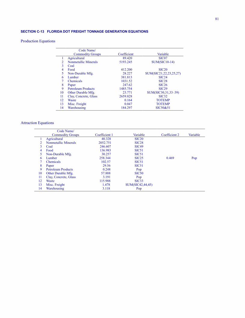
81

SECTION C-13 FLORIDA DOT FREIGHT TONNAGE GENERATION EQUATIONS Production Equations

Code Name/ Commodity Groups Coefficient Variable

1 Agricultural 89.420 SIC07 2 Nonmetallic Minerals 5193.245 SUM(SIC10-14) 3 Coal 4 Food 412.200 SIC20 5 Non-Durable Mfg. 28.227 SUM(SIC21,22,23,25,27) 6 Lumber 381.813 SIC24 7 Chemicals 1031.52 SIC28 8 Paper 247.62 SIC26 9 Petroleum Products 1485.754 SIC29 10 Other Durable Mfg. 23.771 SUM(SIC30,31,33–39) 11 Clay, Concrete, Glass 2659.828 SIC32 12 Waste 0.164 TOTEMP 13 Misc. Freight 0.047 TOTEMP 14 Warehousing 184.297 SIC50&51

Attraction Equations

Code Name/ Commodity Groups Coefficient 1 Variable Coefficient 2 Variable

1 Agricultural 40.328 SIC20 2 Nonmetallic Minerals 2052.751 SIC28 3 Coal 246.607 SIC49 4 Food 136.983 SIC51 5 Non-Durable Mfg. 30.257 SIC51 6 Lumber 258.344 SIC25 0.469 Pop 7 Chemicals 102.57 SIC51 8 Paper 29.56 SIC51 9 Petroleum Products 0.248 Pop 10 Other Durable Mfg. 57.888 SIC50 11 Clay, Concrete, Glass 3.191 Pop 12 Waste 115.988 SIC33 13 Misc. Freight 1.478 SUM(SIC42,44,45) 14 Warehousing 3.118 Pop

THE TRANSPORTATION RESEARCH BOARD is a unit of the National Research Council, a private, nonprofit institution that provides independent advice on scientific and technical issues under a congressional charter. The Research Council is the principal operating arm of the National Academy of Sciences and the National Academy of Engineering. The mission of the Transportation Research Board is to promote innovation and progress in transportation by stimulating and conducting research, facilitating the dissemination of information, and encouraging the implementation of research findings. The Board’s varied activities annually draw on approximately 4,000 engineers, scientists, and other transportation researchers and practitioners from the public and private sectors and academia, all of whom contribute their expertise in the public interest. The program is supported by state transportation departments, federal agencies including the component administrations of the U.S. Department of Transportation, and other organizations and individuals interested in the development of transportation. The National Academy of Sciences is a nonprofit, self-perpetuating society of distinguished scholars engaged in scientific and engineering research, dedicated to the furtherance of science and technology and to their use for the general welfare. Upon the authority of the charter granted to it by the Congress in 1863, the Academy has a mandate that requires it to advise the federal government on scientific and technical matters. Dr. Bruce Alberts is president of the National Academy of Sciences. The National Academy of Engineering was established in 1964, under the charter of the National Academy of Sciences, as a parallel organization of outstanding engineers. It is autonomous in its administration and in the selection of its members, sharing with the National Academy of Sciences the responsibility for advising the federal government. The National Academy of Engineering also sponsors engineering programs aimed at meeting national needs, encouraging education and research, and recognizes the superior achievements of engineers. Dr. William A.Wulf is president of the National Academy of Engineering.

The Institute of Medicine was established in 1970 by the National Academy of Sciences to secure the services of eminent members of appropriate professions in the examination of policy matters pertaining to the health of the public. The Institute acts under the responsibility given to the National Academy of Sciences, by its congressional charter to be an adviser to the federal government and, upon its own initiative, to identify issues of medical care, research, and education. Dr. Kenneth I. Shine is president of the Institute of Medicine. The National Research Council was organized by the National Academy of Sciences in 1916 to associate the broad community of science and technology with the Academy’s purposes of furthering knowledge and advising the federal government. Functioning in accordance with general policies determined by the Academy, the Council has become the principal operating agency of both the National Academy of Sciences and the National Academy of Engineering in providing services to the government, the public, and the scientific and engineering communities. The Council is administered jointly by both Academies and the Institute of Medicine. Dr. Bruce Alberts and Dr. William A. Wulf are chairman and vice chairman, respectively, of the National Research Council.