Brigham Young University Brigham Young University BYU ScholarsArchive BYU ScholarsArchive Theses and Dissertations 2014-06-24 Necessary and Sufficient Conditions for State-Space Network Necessary and Sufficient Conditions for State-Space Network Realization Realization Philip E. Paré Jr. Brigham Young University - Provo Follow this and additional works at: https://scholarsarchive.byu.edu/etd Part of the Computer Sciences Commons BYU ScholarsArchive Citation BYU ScholarsArchive Citation Paré, Philip E. Jr., "Necessary and Sufficient Conditions for State-Space Network Realization" (2014). Theses and Dissertations. 4136. https://scholarsarchive.byu.edu/etd/4136 This Thesis is brought to you for free and open access by BYU ScholarsArchive. It has been accepted for inclusion in Theses and Dissertations by an authorized administrator of BYU ScholarsArchive. For more information, please contact [email protected], [email protected].
Transcript
Brigham Young University Brigham Young University
BYU ScholarsArchive BYU ScholarsArchive
Theses and Dissertations
2014-06-24
Necessary and Sufficient Conditions for State-Space Network Necessary and Sufficient Conditions for State-Space Network
Realization Realization
Philip E. Paré Jr. Brigham Young University - Provo
Follow this and additional works at: https://scholarsarchive.byu.edu/etd
Part of the Computer Sciences Commons
BYU ScholarsArchive Citation BYU ScholarsArchive Citation Paré, Philip E. Jr., "Necessary and Sufficient Conditions for State-Space Network Realization" (2014). Theses and Dissertations. 4136. https://scholarsarchive.byu.edu/etd/4136
This Thesis is brought to you for free and open access by BYU ScholarsArchive. It has been accepted for inclusion in Theses and Dissertations by an authorized administrator of BYU ScholarsArchive. For more information, please contact [email protected], [email protected].
Necessary and Sufficient Conditions for State-Space NetworkRealization
Philip E. PareDepartment of Computer Science, BYU
Master of Science
This thesis presents the formulation and solution of a new problem in systems andcontrol theory, called the Network Realization Problem. Its relationship to other problems,such as State Realization [1] and Structural Identifiability [2], is shown. The motivationfor this work is the desire to completely quantify the conditions for transitioning betweendifferent mathematical representations of linear time-invariant systems. The solution to thisproblem is useful for theorists because it lays a foundation for quantifying the informationcost of identifying a system’s complete network structure from the transfer function.
Keywords: structural identifiability, system identification, linear time-invariant systems
ACKNOWLEDGMENTS
I thank my family for all their help and support, especially my wonderful wife, Annette
and my parents for teaching me to strive for excellence in all that I do. I also thank all
my colleagues in IDeA Labs at Brigham Young University for their friendship and helpful
insights. I thank my advisor, Sean C. Warnick, who has helped me not only with this thesis
but also with my development as a researcher and as a person in general. Finally, I thank my
other thesis committee members – Randal W. Beard, Robert P. Burton, Mark K. Transtrum,
This thesis precisely characterizes the information about (A,B,C,D) that must be known, a
priori, to recover it from G(s), distinct from any of the other minimal realizations of G(s).
Given rich input-output data, system identification algorithms obtain a transfer
function. The problem of State Realization is usually then posed as: given a transfer function,
G(s), find any state-space realization of the system. Different state realization algorithms
give different realizations.
Network structure is how the system is connected together internally, that is, how
the states affect each other, affect the outputs, and are affected by the inputs. The network
structure is revealed by, or encoded in, a set of state-space matrices, (A,B,C,D) that
produced the input-output behavior.The network structure is not necessarily, and is very
unlikely to be equal to an arbitrary minimal realization, (A, B, C, D), that is obtained from
G(s) via a state realization algorithm as discussed above.
The State-Space Network Realization Problem is to identify the internal network
structure of a system, (A,B,C,D), given its transfer function G(s). More precisely, suppose a
state-space system, (A,B,C,D), is fixed and its transfer function, G(s), is given. From G(s)
you can obtain an arbitrary realization, (A, B, C, D) using any state realization algorithm, but
from G(s) alone one cannot tell whether (A, B, C, D) is the given system, (A,B,C,D), that
generated G(s). The question then becomes, what elements of (A,B,C,D), if known a priori,
2
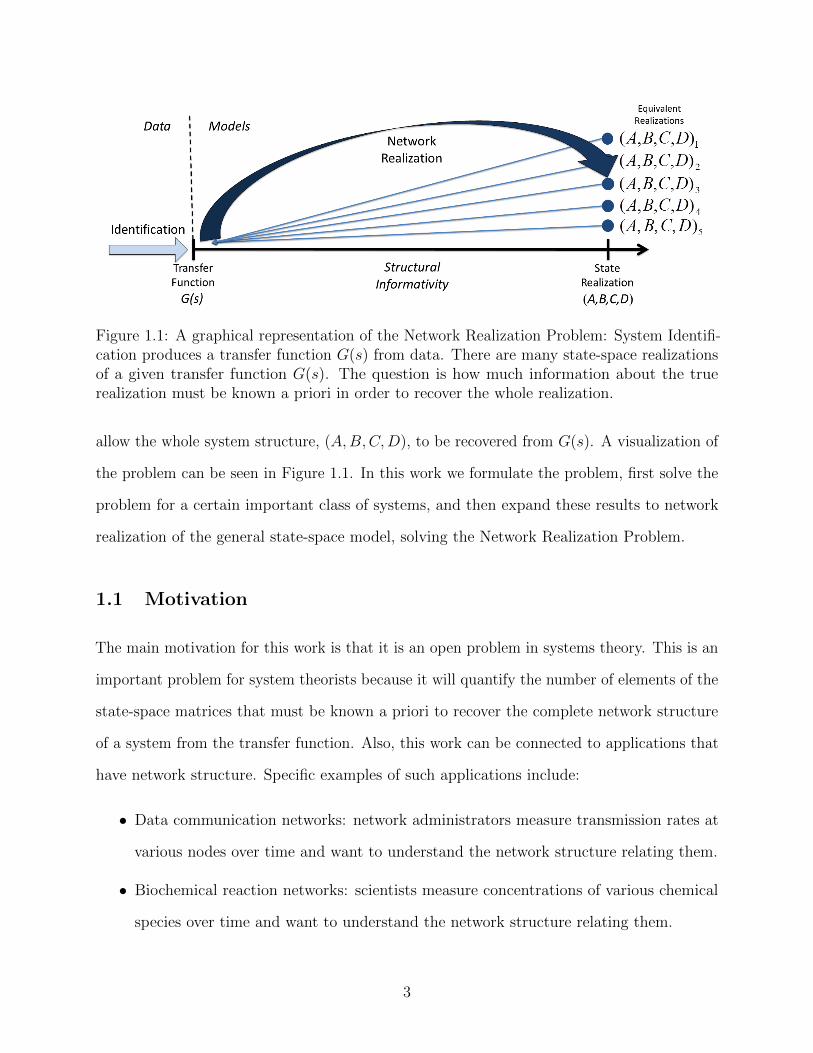
Figure 1.1: A graphical representation of the Network Realization Problem: System Identifi-cation produces a transfer function G(s) from data. There are many state-space realizationsof a given transfer function G(s). The question is how much information about the truerealization must be known a priori in order to recover the whole realization.
allow the whole system structure, (A,B,C,D), to be recovered from G(s). A visualization of
the problem can be seen in Figure 1.1. In this work we formulate the problem, first solve the
problem for a certain important class of systems, and then expand these results to network
realization of the general state-space model, solving the Network Realization Problem.
1.1 Motivation
The main motivation for this work is that it is an open problem in systems theory. This is an
important problem for system theorists because it will quantify the number of elements of the
state-space matrices that must be known a priori to recover the complete network structure
of a system from the transfer function. Also, this work can be connected to applications that
have network structure. Specific examples of such applications include:
• Data communication networks: network administrators measure transmission rates at
various nodes over time and want to understand the network structure relating them.
• Biochemical reaction networks: scientists measure concentrations of various chemical
species over time and want to understand the network structure relating them.
3
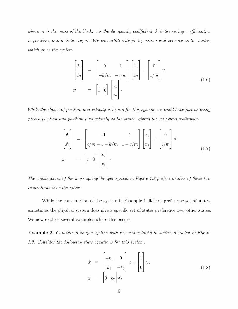
Figure 1.2: This a simple mass spring damper system where m is the mass, c is the dampeningcoefficient, k is the spring coefficient, x is relative position, and u is the input to the system.
• Financial networks: investors measure prices of various securities over time and want
to understand the network structure relating them.
• Social networks: observers measure opinions of various agents on a particular topic over
time and want to understand the network structure relating them.
Although these systems are probably best described by nonlinear dynamics, the theory
developed in this thesis may be applicable to them near equilibria by virtue of Lyapunov’s
Indirect Method [3].
1.1.1 State-Space Realizations vs. Physical Systems
This work focuses on the relationship between the state-space representation of linear time-
invariant systems and the transfer function. This is motivated by the idea that the state-space
model has more physical meaning than the transfer function. However sometimes the physical
interpretation does not specify the states.
Example 1. Consider a simple mass spring damper system, shown in Figure 1.2. The
dynamics are explained by Netwon’s laws,
mx+ cx+ kx = u, (1.5)
4
where m is the mass of the block, c is the dampening coefficient, k is the spring coefficient, x
is position, and u is the input. We can arbitrarily pick position and velocity as the states,
which gives the system
x1x2
=
0 1
−k/m −c/m
x1x2
+
0
1/m
uy =
[1 0
]x1x2
.(1.6)
While the choice of position and velocity is logical for this system, we could have just as easily
picked position and position plus velocity as the states, giving the following realization
x1x2
=
−1 1
c/m− 1− k/m 1− c/m
x1x2
+
0
1/m
uy =
[1 0
]x1x2
.(1.7)
The construction of the mass spring damper system in Figure 1.2 prefers neither of these two
realizations over the other.
While the construction of the system in Example 1 did not prefer one set of states,
sometimes the physical system does give a specific set of states preference over other states.
We now explore several examples where this occurs.
Example 2. Consider a simple system with two water tanks in series, depicted in Figure
1.3. Consider the following state equations for this system,
x =
−k1 0
k1 −k2
x+
1
0
u,y =
[0 k2
]x,
(1.8)
5
Figure 1.3: Two water tanks in series: This simple example illustrates how a system can haveunderlying structure by construction.
where the states are the quantity of water in each tank and the ki’s are the flow rates shown
in Figure 1.3. These states are specified by the construction of the tanks that are in series
and each piece of the system could be separated with each state treated as its own single-state
subsystem. Then the realization in Equation 1.8 shows the interaction between these two
subsystems. The states could be changed to x1 + x2 and x1 − x2 but these cannot be separated
and the realization does not show how the two tanks interact.
The important idea to take from Example 2 is that the construction of the water
tanks specifies a unique set of states unlike the mass spring damper system in Example
1 where neither of the systems in Equations 1.6 and 1.7 can be preferred over the other
due to the physical structure. Since, in Example 2, the construction of the water tanks are
separated and in series, choosing the quantities of water being stored in each tank shows the
interaction of the two subsystems, that is the tanks, and other choices of states do not portray
this structure. In Example 1, the physical construction of the system prefers no state-space
realization over others. We now explore two compartment models of pharmacokinetics that,
similar to Example 2, have structure that prefers a set of states over others.
6
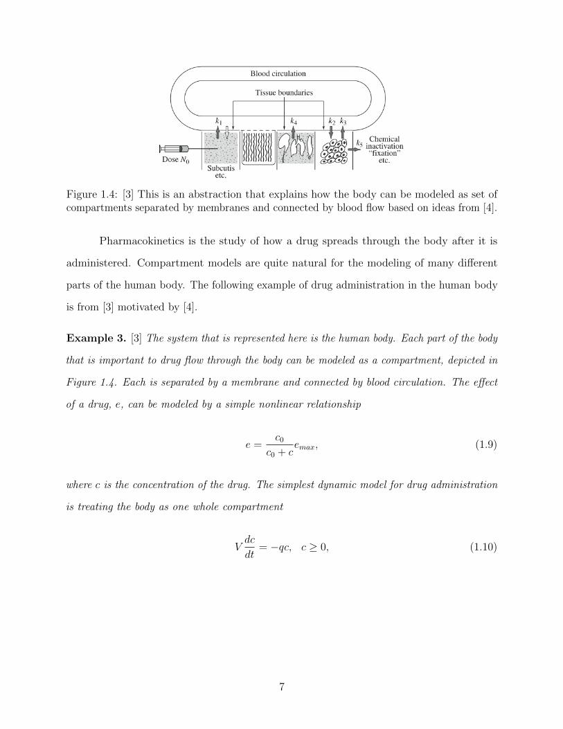
Figure 1.4: [3] This is an abstraction that explains how the body can be modeled as set ofcompartments separated by membranes and connected by blood flow based on ideas from [4].
Pharmacokinetics is the study of how a drug spreads through the body after it is
administered. Compartment models are quite natural for the modeling of many different
parts of the human body. The following example of drug administration in the human body
is from [3] motivated by [4].
Example 3. [3] The system that is represented here is the human body. Each part of the body
that is important to drug flow through the body can be modeled as a compartment, depicted in
Figure 1.4. Each is separated by a membrane and connected by blood circulation. The effect
of a drug, e, can be modeled by a simple nonlinear relationship
e =c0
c0 + cemax, (1.9)
where c is the concentration of the drug. The simplest dynamic model for drug administration
is treating the body as one whole compartment
Vdc
dt= −qc, c ≥ 0, (1.10)
7
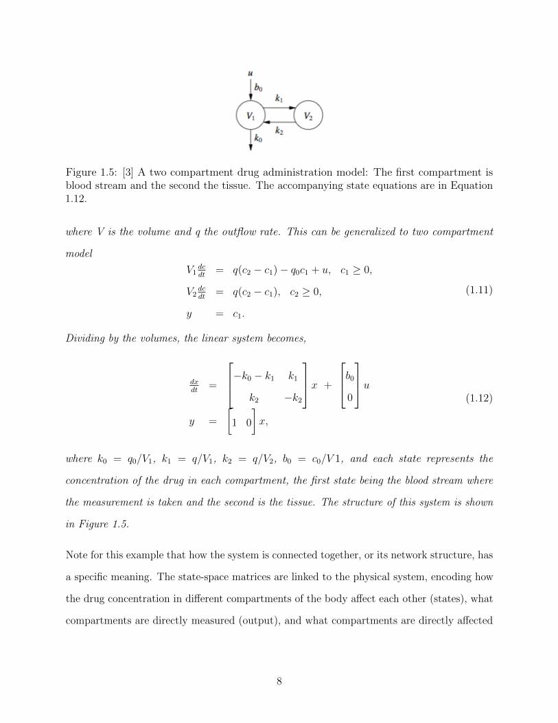
Figure 1.5: [3] A two compartment drug administration model: The first compartment isblood stream and the second the tissue. The accompanying state equations are in Equation1.12.
where V is the volume and q the outflow rate. This can be generalized to two compartment
model
V1dcdt
= q(c2 − c1)− q0c1 + u, c1 ≥ 0,
V2dcdt
= q(c2 − c1), c2 ≥ 0,
y = c1.
(1.11)
Dividing by the volumes, the linear system becomes,
dxdt
=
−k0 − k1 k1
k2 −k2
x +
b00
uy =
[1 0
]x,
(1.12)
where k0 = q0/V1, k1 = q/V1, k2 = q/V2, b0 = c0/V 1, and each state represents the
concentration of the drug in each compartment, the first state being the blood stream where
the measurement is taken and the second is the tissue. The structure of this system is shown
in Figure 1.5.
Note for this example that how the system is connected together, or its network structure, has
a specific meaning. The state-space matrices are linked to the physical system, encoding how
the drug concentration in different compartments of the body affect each other (states), what
compartments are directly measured (output), and what compartments are directly affected
8
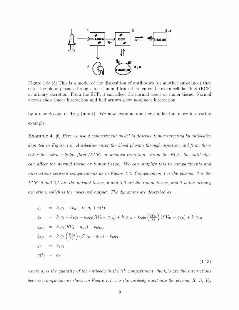
Figure 1.6: [5] This is a model of the disposition of antibodies (or another substance) thatenter the blood plasma through injection and from there enter the extra cellular fluid (ECF)or urinary excretion. From the ECF, it can affect the normal tissue or tumor tissue. Normalarrows show linear interaction and half arrows show nonlinear interaction.
by a new dosage of drug (input). We now examine another similar but more interesting
example.
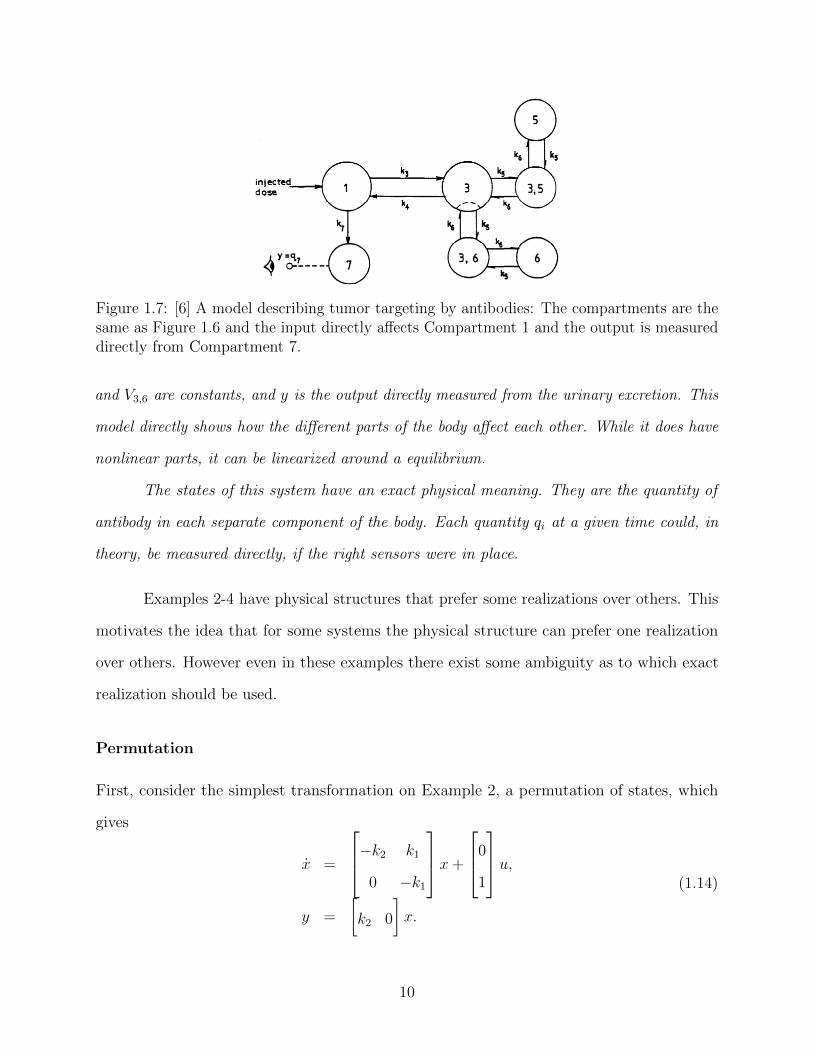
Example 4. [6] Here we use a compartment model to describe tumor targeting by antibodies,
depicted in Figure 1.6. Antibodies enter the blood plasma through injection and from there
enter the extra cellular fluid (ECF) or urinary excretion. From the ECF, the antibodies
can affect the normal tissue or tumor tissue. We can simplify this to compartments and
interactions between compartments as in Figure 1.7. Compartment 1 is the plasma, 3 is the
ECF, 5 and 3,5 are the normal tissue, 6 and 3,6 are the tumor tissue, and 7 is the urinary
excretion, which is the measured output. The dynamics are described as
where qi is the quantity of the antibody in the ith compartment, the ki’s are the interactions
between compartments shown in Figure 1.7, u is the antibody input into the plasma, R, S, V3,
9
Figure 1.7: [6] A model describing tumor targeting by antibodies: The compartments are thesame as Figure 1.6 and the input directly affects Compartment 1 and the output is measureddirectly from Compartment 7.
and V3,6 are constants, and y is the output directly measured from the urinary excretion. This
model directly shows how the different parts of the body affect each other. While it does have
nonlinear parts, it can be linearized around a equilibrium.
The states of this system have an exact physical meaning. They are the quantity of
antibody in each separate component of the body. Each quantity qi at a given time could, in
theory, be measured directly, if the right sensors were in place.
Examples 2-4 have physical structures that prefer some realizations over others. This
motivates the idea that for some systems the physical structure can prefer one realization
over others. However even in these examples there exist some ambiguity as to which exact
realization should be used.
Permutation
First, consider the simplest transformation on Example 2, a permutation of states, which
gives
x =
−k2 k1
0 −k1
x+
0
1
u,y =
[k2 0
]x.
(1.14)
10
This system is clearly equivalent to the system in Equation 1.8 and can be separated as
previously mentioned, still encoding the network structure of the system. So the physical
system cannot distinguish between this realization and the realization in Equation 1.8.
Change of Units
Another ambiguity arises when considering the units of the states. Consider a transformation
of a system that changes the units that the states are measured in but keeps the input-output
behavior the same. This is encoded by a diagonal transformation of the system where X 6= I
(See Equation 1.3). Consider that in Example 2 the states are originally measured in cubic
meters and we change them to cubic feet. This is encoded by the transformation
X =
35.3 0
0 35.5
, (1.15)
giving the system
x =
−k1 0
k1 −k2
x+
35.5
0
u,y =
[0 k2
35.5
]x.
(1.16)
This system is equivalent to the system in Equation 1.8 and still portrays the physical
structure of the system. So the physical system cannot distinguish between this realization
and the realization in Equation 1.8.
Relevance to this Work
It is beyond the scope of this work to tie the physical structure of a system to a specific
state-space realization. However, as is shown in Examples 2-4, the structure of a system can
reduce the set of acceptable realizations. Nevertheless since this is mainly a theoretical piece
of work, as mentioned before, we will assume that there is an underlying system (A,B,C,D)
that created the input-output data and we want to know what information is necessary and
11
sufficient to to recover this system, (A,B,C,D). In so doing, we will solve the Network
Realization Problem.
1.2 Notation
The following is some notation we will use throughout this work:
• In is the n× n identity matrix.
• For a matrix A, AT is its transpose and A−1 is its inverse.
• Given a linear transformation A, the four fundamental subspaces are the range or
column space R(A) = x | Ax = b, the nullspace N(A) = x | Ax = 0, the row
space R(AT ) = b | AT b = x, and the left nullspace N(AT ) = b | AT b = 0 of the
operator A.
• vec(·) stacks the columns of the argument into a vector.
• A⊗B is the Kronecker product of A and B.
• A⊕B is the Kronecker sum of A and B, defined by A⊗ I + I ⊗B.
• A(1 : k, :) indicates that A is truncated to only including the first k rows and all the
columns of A. Similarly, the first k columns of A are denoted by A(:, 1 : k).
• A† is the Moore-Penrose psuedoinverse of A.
12
Chapter 2
Background
2.1 Background
Model classes are parameterized sets of models that attempt to constrain manifest variables
in a manner consistent with our observations or beliefs about how a system behaves. Learning
problems choose a particular element of this set, indexed by a unique vector of parameters,
that best explains our observational data.
In this work, G(s) represents our observational data, and the minimal state-space
realizations of G(s) is the model class of interest. We assume no noise, that is to say, we
assume that the network structure, (A,B,C,D), is the system that generated G(s) is, in fact,
one of its minimal realizations. Our problem is to characterize the conditions when we can
recover (A,B,C,D) from G(s).
Solving this problem begins with the characterization of the appropriate model
class. In this work, we begin with a state-space model as in Equation (1.1), so we start
by parameterizing all systems of this form. We then define subsets of this model class
characterized by fixing certain “known” elements of (A,B,C,D).
Definition 1. [2] A general parameterization of the system defined by Equation (1.1) is a
continuously differentiable function P (α) : Ω ⊂ Rq → RN , where q is the number of unknown
parameters, N = n(n+m+ p) +mp, and Ω is a set of admissible values of the parameters.
A general parameterization allows one to choose q parameters depicted by α, and it will
return P (α) = β ∈ R(P ) ⊆ RN where N = n(n + m + p) + mp. Each element of RN
13
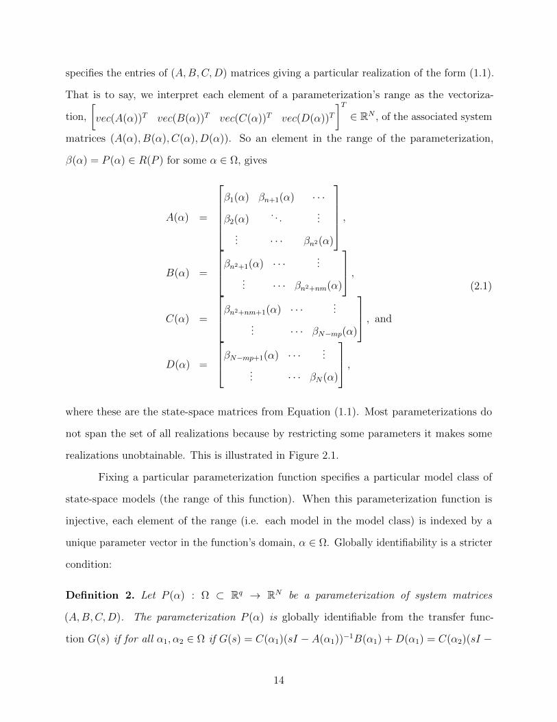
specifies the entries of (A,B,C,D) matrices giving a particular realization of the form (1.1).
That is to say, we interpret each element of a parameterization’s range as the vectoriza-
tion,
[vec(A(α))T vec(B(α))T vec(C(α))T vec(D(α))T
]T∈ RN , of the associated system
matrices (A(α), B(α), C(α), D(α)). So an element in the range of the parameterization,
β(α) = P (α) ∈ R(P ) for some α ∈ Ω, gives
A(α) =
β1(α) βn+1(α) · · ·
β2(α). . .
...
... · · · βn2(α)
,
B(α) =
βn2+1(α) · · · ...
... · · · βn2+nm(α)
,C(α) =
βn2+nm+1(α) · · · ...
... · · · βN−mp(α)
, and
D(α) =
βN−mp+1(α) · · · ...
... · · · βN(α)
,
(2.1)
where these are the state-space matrices from Equation (1.1). Most parameterizations do
not span the set of all realizations because by restricting some parameters it makes some
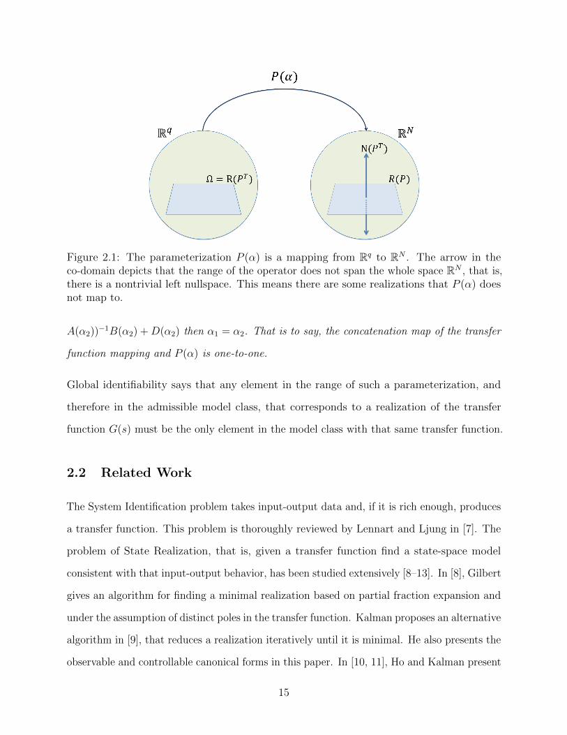
realizations unobtainable. This is illustrated in Figure 2.1.
Fixing a particular parameterization function specifies a particular model class of
state-space models (the range of this function). When this parameterization function is
injective, each element of the range (i.e. each model in the model class) is indexed by a
unique parameter vector in the function’s domain, α ∈ Ω. Globally identifiability is a stricter
condition:
Definition 2. Let P (α) : Ω ⊂ Rq → RN be a parameterization of system matrices
(A,B,C,D). The parameterization P (α) is globally identifiable from the transfer func-
tion G(s) if for all α1, α2 ∈ Ω if G(s) = C(α1)(sI − A(α1))−1B(α1) +D(α1) = C(α2)(sI −
14
Figure 2.1: The parameterization P (α) is a mapping from Rq to RN . The arrow in theco-domain depicts that the range of the operator does not span the whole space RN , that is,there is a nontrivial left nullspace. This means there are some realizations that P (α) doesnot map to.
A(α2))−1B(α2) +D(α2) then α1 = α2. That is to say, the concatenation map of the transfer
function mapping and P (α) is one-to-one.
Global identifiability says that any element in the range of such a parameterization, and
therefore in the admissible model class, that corresponds to a realization of the transfer
function G(s) must be the only element in the model class with that same transfer function.
2.2 Related Work
The System Identification problem takes input-output data and, if it is rich enough, produces
a transfer function. This problem is thoroughly reviewed by Lennart and Ljung in [7]. The
problem of State Realization, that is, given a transfer function find a state-space model
consistent with that input-output behavior, has been studied extensively [8–13]. In [8], Gilbert
gives an algorithm for finding a minimal realization based on partial fraction expansion and
under the assumption of distinct poles in the transfer function. Kalman proposes an alternative
algorithm in [9], that reduces a realization iteratively until it is minimal. He also presents the
observable and controllable canonical forms in this paper. In [10, 11], Ho and Kalman present
15
an alternative algorithm similar to [9] in that it iterates but it uses the Markov parameters
instead of the transfer function. A thorough overview of the Minimal State Realization
Problem is provided in [1].
The work done by Ho and Kalman in [10, 11] led to another problem called Subspace
Identification. This problem takes input-output data and produces the Hankel operator,
which is a matrix of the Markov parameters, and factors it into the observability and
controllability grammians, which are then used to obtain a minimal state-space realization.
Subspace Identification can be thought of as an alternative to the combination of the System
Identification and the State Realization Problems because it goes from input-output data
to a state-space model, but it differs in that it avoids the frequency domain. Similar to
State Realization, Subspace Identification finds any state-space model consistent with the
input-output behavior of the Hankel operator, that is to say, different subspace identification
algorithms produce different state-space realizations and the likelihood that the realization
produced by the algorithm is (A,B,C,D), or the network structure, sought by the Network
Realization Problem is very low. Subspace identification gives no insight into finding the
state transformation from an arbitrary realization to the network structure.
In [14], Kung proposed the first modification of [10, 11], using the singular value
decomposition (SVD) of the estimated Hankel operator. In [15], Juang presents the eigen-
system realization approach, which uses a truncation of the SVD of the Hankel operator
to obtain a state-space model, and verifies it using data from the Galileo spacecraft. In
[16–18], a realization algorithm is presented that matches measurements of impulse response
parameters and the auto-covariance of the output to their corresponding models to provide a
parameterization of all minimal stable realizations. At the end of [16] they explicitly state
that a “method to choose a specific realization to satisfy other modeling considerations has
not been determined.” The work here addresses this problem. In [19], Van Der Veen uses
both known and new subspace identification algorithms that employ SVD to discriminate
16
between desired and noisy signals. A good overview of Subspace Identification is provided in
[20].
There is some confusion, or perhaps lack of rigor at times, surrounding Subspace
Identification. In [21], when they formulate the problem they say, given input-output data,
find the order n and the state-space matrices in Equation (1.1). This is not what Subspace
Identification does; it finds a set of state-space matrices (A, B, C, D), but not the exact ones
that produced the data (A,B,C,D). The two are related by a state transformation but are
different. In order to recover the exact matrices (A,B,C,D) that produced the input-output
data some a priori knowledge of the matrices is required, which Subspace Identification does
not assume.
The Network Realization Problem, the State Realization Problem, and Subspace
Identification are all related to the problem of Structural Identifiability, which is the ability
to identify the internal network structure of a system given that you know some underlying
structure of the system. This allows the problem to be posed more generally but does not
enable necessary and sufficient conditions for global identifiability. Bellman and Astrom
introduce and formulate this problem in [22]. They also present the necessary and sufficient
conditions for several classes of systems; including single–input single–output single–state,
Rothenberg provides conditions for local identifiability for a general stochastic model in
[23] which depends on the non-singularity of the information matrix. In [2], Glover and
Willems provide necessary and sufficient conditions for local identifiability. They also provide
a sufficient condition for global identifiability but fail to provide necessary conditions. In [24],
Milanese provides necessary and sufficient conditions for observability of an unidentifiable
parameterization. A great discussion on the different definitions of parameter and structural
identifiability is provided in [25]. The Structural Identifiability problem can be motivated by
several physiology applications in [26].
17
The theory for structural identifiability was originally developed in the 1970’s. However,
the expansion of research in the field of Systems Biology ([27]) over the last twenty five years
has begun to highlight the importance of the identifiability results as shown in [6, 28–32].
These papers try to recover the network structure of systems in the applications of kinetics
of substances like drugs and tracers, biochemical reaction networks, pancreatic cancer, and
metabolic networks.
Another piece of related work is the dynamical structure function (DSF), introduced
in [33]. This is a dynamic multi-scale representation of systems, that scales with the number
of measured states. If one state is measured, the DSF is the transfer function. If all the
states are measured, it provides a representation that is equivalent to the state-space matrices.
Since structural information is encoded in the representation, some a priori knowledge of the
structure is required for reconstruction similar to the state-space matrices. The necessary
and sufficient conditions for reconstruction of the DSF from the transfer function are given
in [34, 35]. These results differ from this work because they provide conditions for recovering
the DSF from the transfer function while this work provides conditions for recovering the
state-space matrices from the transfer function.
2.3 Thesis Contribution
In this work, we provide necessary and sufficient conditions for global identifiability from
the transfer function for a specific type of parameterization, which solves the Network
Realization Problem. Because we provide necessary and sufficient conditions for a certain
type of parameterization, this problem can be thought of as a sub-problem of the Structural
Identifiability Problem.
18
Chapter 3
Problem Formulation
For the Network Realization problem we focus on a specific type of parameterization
that enables us to fix the known elements of the network structure, represented by (A,B,C,D).
In order to formulate the problem we present essential definitions that refine Definition 1.
Definition 3. The identity parameterization I(θ) : RN → RN , where N = n(n+m+p)+mp,
maps θ to itself where θ is a vectorization of the system matrices,
θ =
[vec(A)T vec(B)T vec(C)T vec(D)T
]T, so that the parameters in θ are exactly the
elements of the system matrices, stacked appropriately.
Definition 4. Let f : X → Y be a function from a set X to a set Y. If F is a subset of X ,
then the restriction of f to F is the function
f |F : F → Y , (3.1)
meaning f |F(x) = f(x) ∀x ∈ F ⊂ X .
Definition 5. Consider f : X → Y for some linear vector spaces X and Y, and let B =
b1, b2, ..., br, ... be a basis of X with indicator function ΘR. Let R = spanb1, b2, ..., br ⊂ X
and F = X/R. Then, for some θ∗R ∈ R ⊂ X , the restriction of f given by
f |θ∗R+F = θ∗R + F → Y (3.2)
19
is called affine, and we write f |θ∗R(θF), where θF ∈ F , to mean f |θ∗R+F. Moreover, the basis
elements b1, b2, ..., br are called restricted, while the rest of the basis elements are called
free.
ΘR is a binary vector that indicates which coordinates of X are restricted. θ∗R is a vector in
X with specific values for the restricted coordinates and zeros in the positions of the free
coordinates. In this way, θ∗R encodes the information about a fixed realization, (A,B,C,D),
that is known a priori. Likewise, θF is a vector in X with specific values for the free coordinates
and zeros in the positions of the restricted coordinates. Sometimes we abuse notation by
eliminating the zeros in the positions of the restricted coordinates of θF , and view it as an
element of F , not as an element of F embedded in X . The following example illustrates the
restriction of the identity parameterization.
Example 5. Consider the system characterized by the state equations
x = ax+ bu
y = cx.(3.3)
The identity parameterization takes a vector in R3 and associates a particular system with it,
so θ = [−1 1 2]T becomes
x = −x+ u
y = 2x.(3.4)
The restriction of the identity given by I|[0 0 0]T (θF), with ΘR = [1 0 0]T , generates the class
of systems parameterized by θF = [0 b c]T (or, equivalently, θF = [b c]T ) as
x = bu
y = cx.(3.5)
20
While the restriction of the identity given by I|[−3 0 5]T (θF), with ΘR = [1 0 1]T , generates the
class of systems parameterized by θF = [0 b 0]T (or, equivalently, θF = b) as
x = −3x+ bu
y = 5x.(3.6)
Definition 6. Consider a system (A,B,C,D) given by Equation (1.1), and let
θ∗ =
[vec(A)T vec(B)T vec(C)T vec(D)T
]T. An affine restriction of the identity parame-
trization, I|θ∗R, with arguments characterized by F , is consistent with θ∗ (or (A,B,C,D)) if
there exists some θF ∈ F such that θ∗ = θ∗R + θF . In other words, I|θ∗R is consistent with θ∗
if θ∗ ∈ R(I|θ∗R), the range of the parameterization I|θ∗R.
Thus, a restriction of the identity is consistent with a particular system if the restricted
parameters and the associated values in the system’s state representation are equal.
Lemma 1. If I|θ∗R is consistent with two unequal realizations with the same transfer function
G(s) then I|θ∗R is not globally identifiable from G(s).
Proof. Assume I|θ∗R is consistent with θ1 and θ2, θ1 6= θ2, with the same transfer function G(s).
This means there exist θF1 , θF2 ∈ F , θF1 6= θF2 , where θ1 = I|θ∗R(θF1) and θ2 = I|θ∗R(θF2),
such that G(s) = C(θF1)(sI − A(θF1))−1B(θF1) = C(θF2)(sI − A(θF2))
−1B(θF2). But since
θ1 6= θ2, then by definition I|θ∗R is not globally identifiable from G(s).
3.1 Problem Statement
Loosely speaking, our objective is to characterize the conditions under which one can recover
(A,B,C,D) from knowledge of its transfer function. This goal is made precise in the following
problem formulation.
State-Space Network Realization Problem. Consider a system (A,B,C,D) as in
Equation (1.1), with (A,B) controllable and (A,C) observable, and suppose
21
G(s) = C(sI−A)−1B+D is given. Find an affine restriction of the identity parameterization,
I|θ∗R, consistent with (A,B,C,D), that is globally identifiable from G(s).
Note that the identity parameterization is not globally identifiable from any G(s) by Lemma
1, since every G(s) has multiple realizations and I(θ) is consistent with all of them. Finding
a consistent affine restriction that is globally identifiable means identifying θ∗R, or elements of
(A,B,C,D), that, if known, enable one to recover the rest of (A,B,C,D) from G(s).
3.2 Parameterization Example
This example illustrates global identifiability and the Network Realization Problem.
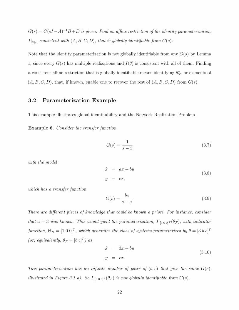
Example 6. Consider the transfer function
G(s) =1
s− 3(3.7)
with the model
x = ax+ bu
y = cx,(3.8)
which has a transfer function
G(s) =bc
s− a. (3.9)
There are different pieces of knowledge that could be known a priori. For instance, consider
that a = 3 was known. This would yield the parameterization, I|[3 0 0]T (θF), with indicator
function, ΘR = [1 0 0]T , which generates the class of systems parameterized by θ = [3 b c]T
(or, equivalently, θF = [b c]T ) as
x = 3x+ bu
y = cx.(3.10)
This parameterization has an infinite number of pairs of (b, c) that give the same G(s),
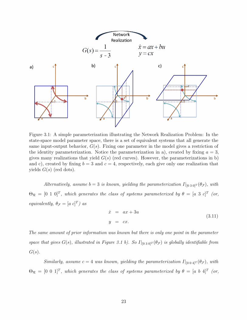
illustrated in Figure 3.1 a). So I|[3 0 0]T (θF) is not globally identifiable from G(s).
22
Figure 3.1: A simple parameterization illustrating the Network Realization Problem: In thestate-space model parameter space, there is a set of equivalent systems that all generate thesame input-output behavior, G(s). Fixing one parameter in the model gives a restriction ofthe identity parameterization. Notice the parameterization in a), created by fixing a = 3,gives many realizations that yield G(s) (red curves). However, the parameterizations in b)and c), created by fixing b = 3 and c = 4, respectively, each give only one realization thatyields G(s) (red dots).
Alternatively, assume b = 3 is known, yielding the parameterization I|[0 3 0]T (θF), with
ΘR = [0 1 0]T , which generates the class of systems parameterized by θ = [a 3 c]T (or,
equivalently, θF = [a c]T ) as
x = ax+ 3u
y = cx.(3.11)
The same amount of prior information was known but there is only one point in the parameter
space that gives G(s), illustrated in Figure 3.1 b). So I|[0 3 0]T (θF) is globally identifiable from
G(s).
Similarly, assume c = 4 was known, yielding the parameterization I|[0 0 4]T (θF), with
ΘR = [0 0 1]T , which generates the class of systems parameterized by θ = [a b 4]T (or,
23
equivalently, θF = [a b]T ) as
x = ax+ bu
y = 4x.(3.12)
Again, there is only one point in the parameter space that gives G(s), illustrated in Figure 3.1
c). So I|[0 0 4]T (θF) is globally identifiable from G(s).
For this example one can immediately see that a = 3 because 3 is the unique pole of G(s).
So knowing a priori that a = 3 offers no new information, while the other cases do offer new
information to specify the true system. In general, knowing A a priori is never sufficient to
recover the network structure of the system.
Also note that the first parameterization in Example 6 was not globally identifiable
from G(s). However the second two were, and all three of the parameterizations only restricted
one element. Therefore, for global identifiability, the value of the a priori information is not
necessarily quantified by the amount of information.
24
Chapter 4
Direct–State Measurement
A special case of this problem is published in [36]. The specific class of systems
considered is
x(t) = Ax(t) +Bu(t)
y(t) = [ Ip 0 ]x(t),(4.1)
where a set of the states are directly measured. This chapter focuses on restrictions of
the identity parameterization that only fix the elements in the C matrix and fixes them to
C = [Ip 0], which is denoted by I|C . This class of systems is important for various applications
including biochemical reaction networks where scientists are directly measuring some of the
chemical species in a mixture [30].
4.1 Global Identifiability of State Measurement Systems
The following theorem statement is changed slightly from [36] to match the parameterization
notation.
Theorem 1. [36] The restriction of the identity parameterization I|C=[Ip 0], where no elements
of A and B are fixed, is globally identifiable from G(s) if and only if p = n.
Proof. (⇒) We prove necessity by contraposition. By the structure of C in Equation (4.1),
p ≤ n where if p = n then C = I. In other words, p > n is not permissible for this model
class.
25
Assume p < n. This implies C =
[Ip 0n−p
]with n− p > 0, thus C 6= I. Moreover,
for any system there exists a minimal pair of matrices (A,B), not necessarily unique, that
realize G(s):
G(s) = C(sI − A)−1B. (4.2)
Consider the state transformation X and its inverse:
X =
In 0
K In−p
, X−1 =
In 0
−K In−p
, (4.3)
where K is an arbitrary (n− p)× n nonzero matrix.
The resulting transformed system, A = XAX−1, B = XB, and C = CX−1, is
still of the form (4.1), since CX−1 = C, and clearly has the same transfer function G(s).
Nevertheless, different values of K will clearly result in various dynamics matrices, A, and
control matrices, B, thus showing that p < n implies that I|C is consistent with multiple
minimal realizations that give G(s). Therefore I|C is not globally identifiable from G(s).
(⇐) Assume n = p, C = I and that G(s) is realized by (A1, B1, C1) and (A2, B2, C2)
in the range of I|C=I . This implies the existence of an invertible matrix X such that
A2 = XA1X−1, B2 = XB1, and C2 = C1X
−1. Since C1 = C2 = I and C2 = C1X−1 the only
acceptable X matrix is clearly the identity matrix. Therefore A1 = A2 and B1 = B2 and only
one set of matrices (A,B) realizes G(s) in the range of I|C=I . So I|C=I is globally identifiable
from G(s).
This theorem states that network structure cannot be recovered for the class of models
depicted in Equation (4.1), assuming nothing is known about A and B, unless C = I. This
assumption is unrealistic for in vivo biochemical reaction networks because it is impossible to
measure all chemical species in a mixture for an uncontrolled environment.
26
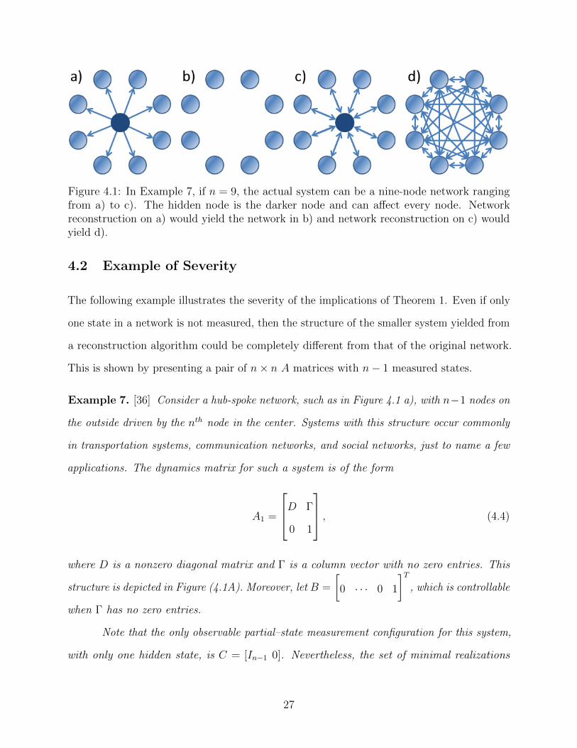
Figure 4.1: In Example 7, if n = 9, the actual system can be a nine-node network rangingfrom a) to c). The hidden node is the darker node and can affect every node. Networkreconstruction on a) would yield the network in b) and network reconstruction on c) wouldyield d).
4.2 Example of Severity
The following example illustrates the severity of the implications of Theorem 1. Even if only
one state in a network is not measured, then the structure of the smaller system yielded from
a reconstruction algorithm could be completely different from that of the original network.
This is shown by presenting a pair of n× n A matrices with n− 1 measured states.
Example 7. [36] Consider a hub-spoke network, such as in Figure 4.1 a), with n−1 nodes on
the outside driven by the nth node in the center. Systems with this structure occur commonly
in transportation systems, communication networks, and social networks, just to name a few
applications. The dynamics matrix for such a system is of the form
A1 =
D Γ
0 1
, (4.4)
where D is a nonzero diagonal matrix and Γ is a column vector with no zero entries. This
structure is depicted in Figure (4.1A). Moreover, let B =
[0 · · · 0 1
]T, which is controllable
when Γ has no zero entries.
Note that the only observable partial–state measurement configuration for this system,
with only one hidden state, is C = [In−1 0]. Nevertheless, the set of minimal realizations
27
clearly preserves the same partial state configuration (i.e. preserve C = [In−1 0]) span all
possible Boolean structures for the dynamics matrix.
To see this, consider the state transformation T =
In−1 0
ΓT 1
. The new, transformed
dynamics matrix then becomes:
A2 = TA1T−1 =
In−1 0
ΓT 1
D Γ
0 1
In−1 0
−Γ 1
=
D Γ
ΓT ∗
In−1 0
−ΓT 1
=
Γ ∗
∗ ∗
(4.5)
where ∗ indicates a nonzero entry of the appropriate dimension. The non-diagonal entries
of Γ are equal to γij = di − γiγj = di − ij, which is nonzero by the construction of Γ. This
results in the structure shown in Figure 4.1 c). Notice that C = CT−1, demonstrating that
this state transformation preserves the partial state configuration of the system.
Clearly the transfer functions for both systems are equal, since they differ only by
a state transformation. Nevertheless, notice that the portion of the underlying realization
corresponding to the measured states, i.e. the sub matrix Γ in the transformed system, can
have any Boolean structure, from diagonal, as in Equation (4.4), to completely full, as in
Equation (4.5) (or anything in between). Thus, any network reconstruction technique that
attempts to recover this system–even knowing a priori that the system is both controllable and
observable–cannot distinguish even the Boolean structure relating the measured nodes to each
other without more information than the input-output behavior of the system.
From Example 7 we can see that even if a network had 1000 states, and we missed
measuring only a single hidden state, then a reconstruction method may reasonably recover
a full network, like Figure 4.1 d), where it could actually have been completely disconnected,
like Figure 4.1 b), or vice versa.
28
Chapter 5
General System State-Space Network Realization
In Chapter 4 we solved the Network Realization Problem for the specific state-space
system where C = [I 0]. However, this result did not give a general solution to Problem 3.1.
This chapter expands the solution from Chapter 4 to the general state-space system given in
Equation (1.1), solving the Network Realization Problem (3.1).
The key idea for the solution technique is the fact, that for a minimal system, every
possible vector of parameters in the domain of a restriction of the parameterization, I|θ∗R ,
maps to a system that can be related to any other realization of G(s) by a non-singular state
transformation X. In Chapter 4, this fact was exploited to provide necessary and sufficient
conditions for direct–state measurement systems. We now generalize this idea for generic
systems.
5.1 Solution to the Network Realization Problem
Definition 7. A restriction of the identity parameterization, I|θ∗R, and a realization,
(A, B, C, D), are compatible if there exists a θ = I|θ∗R(θF) ∈ R(I|θ∗R) (i.e. I|θ∗R consistent with
θ) such that C(sI − A)−1B + D = C(θF)(sI − A(θF))−1B(θF) +D(θF).
Definition 6 explains that a particular state-space model, (A,B,C,D), is consistent with
a given restriction of the identity parameterization, I|θ∗R , if the elements of (A,B,C,D)
corresponding to the restricted elements in the indicator function ΘR are set to the values in
29
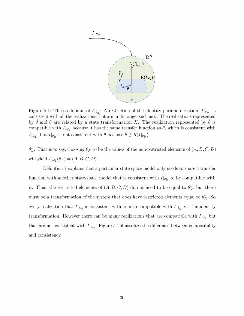
Figure 5.1: The co-domain of I|θ∗R : A restriction of the identity parameterization, I|θ∗R , isconsistent with all the realizations that are in its range, such as θ. The realizations representedby θ and θ are related by a state transformation X. The realization represented by θ iscompatible with I|θ∗R because it has the same transfer function as θ, which is consistent with
I|θ∗R , but I|θ∗R is not consistent with θ because θ /∈ R(I|θ∗R).
θ∗R. That is to say, choosing θF to be the values of the non-restricted elements of (A,B,C,D)
will yield I|θ∗R(θF) = (A,B,C,D).
Definition 7 explains that a particular state-space model only needs to share a transfer
function with another state-space model that is consistent with I|θ∗R to be compatible with
it. Thus, the restricted elements of (A,B,C,D) do not need to be equal to θ∗R, but there
must be a transformation of the system that does have restricted elements equal to θ∗R. So
every realization that I|θ∗R is consistent with, is also compatible with I|θ∗R via the identity
transformation. However there can be many realizations that are compatible with I|θ∗R but
that are not consistent with I|θ∗R . Figure 5.1 illustrates the difference between compatibility
and consistency.
30
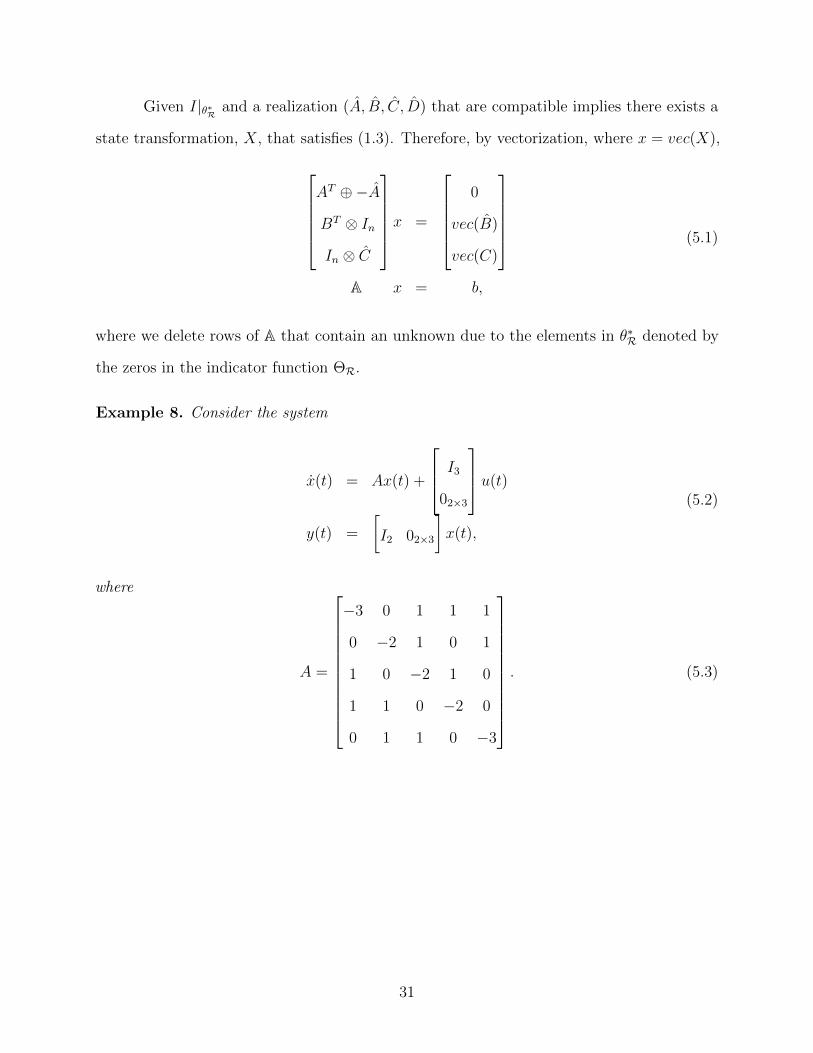
Given I|θ∗R and a realization (A, B, C, D) that are compatible implies there exists a
state transformation, X, that satisfies (1.3). Therefore, by vectorization, where x = vec(X),
AT ⊕−A
BT ⊗ In
In ⊗ C
x =
0
vec(B)
vec(C)
A x = b,
(5.1)
where we delete rows of A that contain an unknown due to the elements in θ∗R denoted by
the zeros in the indicator function ΘR.
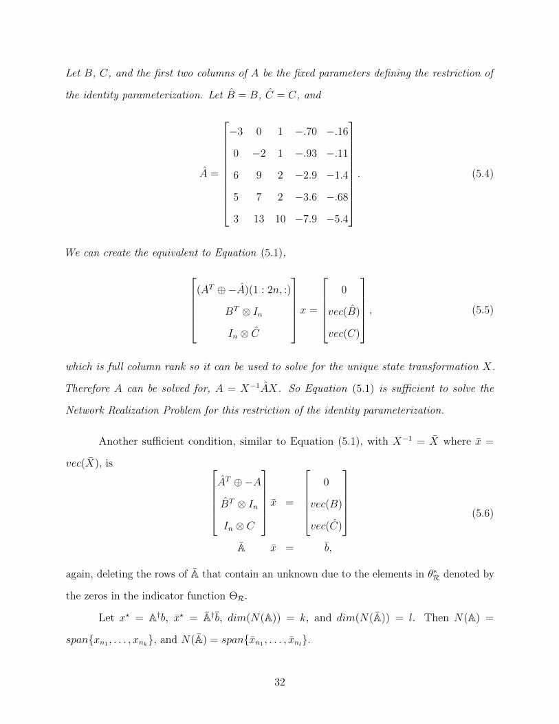
Example 8. Consider the system
x(t) = Ax(t) +
I3
02×3
u(t)
y(t) =
[I2 02×3
]x(t),
(5.2)
where
A =
−3 0 1 1 1
0 −2 1 0 1
1 0 −2 1 0
1 1 0 −2 0
0 1 1 0 −3
. (5.3)
31
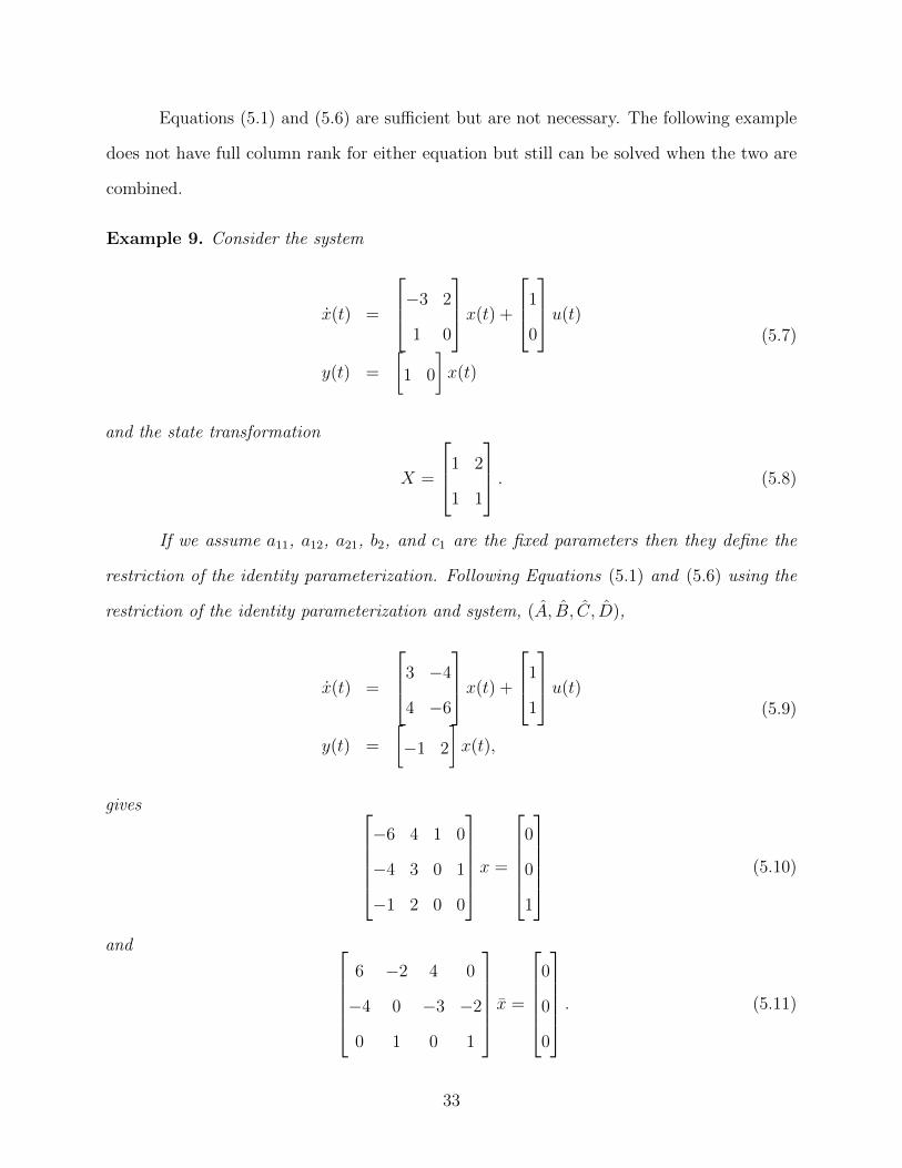
Let B, C, and the first two columns of A be the fixed parameters defining the restriction of
the identity parameterization. Let B = B, C = C, and
A =
−3 0 1 −.70 −.16
0 −2 1 −.93 −.11
6 9 2 −2.9 −1.4
5 7 2 −3.6 −.68
3 13 10 −7.9 −5.4
. (5.4)
We can create the equivalent to Equation (5.1),
(AT ⊕−A)(1 : 2n, :)
BT ⊗ In
In ⊗ C
x =
0
vec(B)
vec(C)
, (5.5)
which is full column rank so it can be used to solve for the unique state transformation X.
Therefore A can be solved for, A = X−1AX. So Equation (5.1) is sufficient to solve the
Network Realization Problem for this restriction of the identity parameterization.
Another sufficient condition, similar to Equation (5.1), with X−1 = X where x =
vec(X), is AT ⊕−A
BT ⊗ In
In ⊗ C
x =
0
vec(B)
vec(C)
A x = b,
(5.6)
again, deleting the rows of A that contain an unknown due to the elements in θ∗R denoted by
the zeros in the indicator function ΘR.
Let x? = A†b, x? = A†b, dim(N(A)) = k, and dim(N(A)) = l. Then N(A) =
Figure 5.2 explains the relationship between Equations (5.1), (5.6), and (5.14).
34
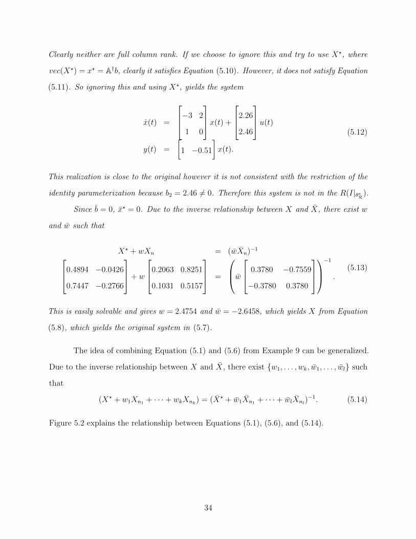
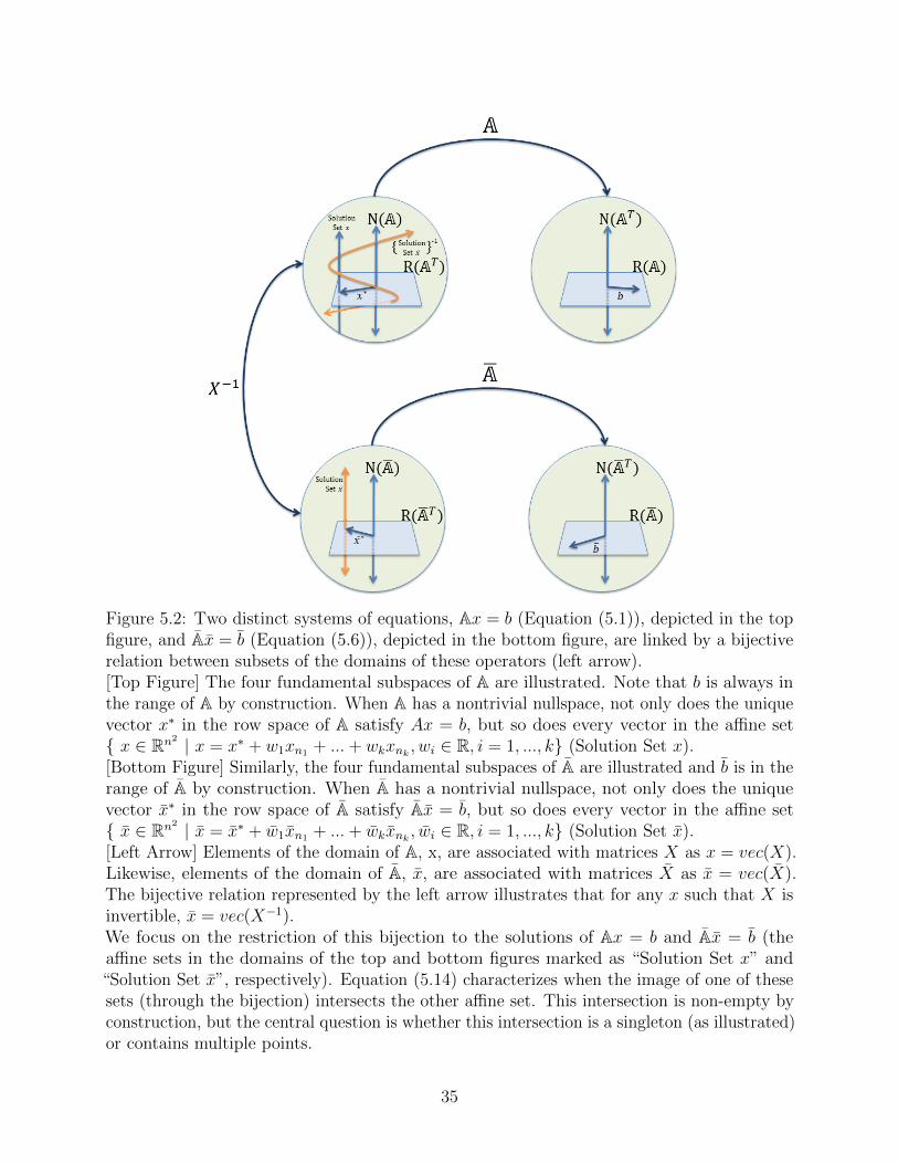
Figure 5.2: Two distinct systems of equations, Ax = b (Equation (5.1)), depicted in the topfigure, and Ax = b (Equation (5.6)), depicted in the bottom figure, are linked by a bijectiverelation between subsets of the domains of these operators (left arrow).[Top Figure] The four fundamental subspaces of A are illustrated. Note that b is always inthe range of A by construction. When A has a nontrivial nullspace, not only does the uniquevector x∗ in the row space of A satisfy Ax = b, but so does every vector in the affine set x ∈ Rn2 | x = x∗ + w1xn1 + ...+ wkxnk
, wi ∈ R, i = 1, ..., k (Solution Set x).[Bottom Figure] Similarly, the four fundamental subspaces of A are illustrated and b is in therange of A by construction. When A has a nontrivial nullspace, not only does the uniquevector x∗ in the row space of A satisfy Ax = b, but so does every vector in the affine set x ∈ Rn2 | x = x∗ + w1xn1 + ...+ wkxnk
, wi ∈ R, i = 1, ..., k (Solution Set x).[Left Arrow] Elements of the domain of A, x, are associated with matrices X as x = vec(X).Likewise, elements of the domain of A, x, are associated with matrices X as x = vec(X).The bijective relation represented by the left arrow illustrates that for any x such that X isinvertible, x = vec(X−1).We focus on the restriction of this bijection to the solutions of Ax = b and Ax = b (theaffine sets in the domains of the top and bottom figures marked as “Solution Set x” and“Solution Set x”, respectively). Equation (5.14) characterizes when the image of one of thesesets (through the bijection) intersects the other affine set. This intersection is non-empty byconstruction, but the central question is whether this intersection is a singleton (as illustrated)or contains multiple points.
35
5.1.1 Main Result
The previous machinery leads to the following theorem statement.
Theorem 2. (Main Result)
1. Given a proper transfer function, G(s), with two minimal realizations, S = (A,B,C,D)
and S = (A, B, C, D), each as in Equation (1.1).
2. Suppose part of S is known, specified by the entries of θ∗R ∈ RN and the indicator
function ΘR, characterizing the affine restriction of the identity parameterization I|θ∗R.
3. Suppose all of S is known.
4. Note that I|θ∗R and S are compatible, thereby specifying A, b, A, b, X∗, Xni, X∗, Xnj
,
i = 1, ..., k, j = 1, ..., l according to Equations (5.1), (5.6), and (5.14).
Then I|θ∗R is globally identifiable from G(s) if and only if Equation (5.14) has a unique
solution.
Proof. Since I|θ∗R is consistent with S, and compatible with S there is at least one solution
to (5.14).
(⇒) We prove this by contraposition. The negation of the statement, “Equation (5.14)
has a unique solution,” is, “Equation (5.14) has no solution or it has multiple solutions.”
However, since there is at least one solution to (5.14), we assume (5.14) has two solutions,
w1, . . . , wk, w1, . . . , wl 6= v1, . . . , vk, v1, . . . , vl. Since the set xn1 , . . . , xnk is linearly
independent by construction, there exist X1, X2, where X1 = X? + w1Xn1 + · · ·+ wkXnk6=
X2 = X? + v1Xn1 + · · · + vkXnk. This implies that I|θ∗R is consistent with two non-equal
realizations, (A1, B1, C1, D1) 6= (A2, B2, C2, D2), where A1 = X−11 AX1 and A2 = X−12 AX2
and G(s) = C(sI−A))−1B+D = C1(sI−A1)−1B1 +D1 = C2(sI−A2)
−1B2 +D2. Therefore,
by Lemma 1, I|θ∗R is not globally identifiable from G(s).
(⇐) Assume (5.14) has a unique solution w1, . . . , wk, w1, . . . , wl. This implies there
is a unique matrix X = X? + w1Xn1 + · · · + wkXnk, with X−1 well defined, such that X
36
satisfies Equation (5.1) and X−1 satisfies Equation (5.6). The fact that X is invertible implies
that X is a valid state transformation from S to another system S, that is
A = X−1AX, B = X−1B, C = CT, and D = D.
Moreover, since vec(X) satisfies Equation (5.1) and vec(X−1) satisfies Equation (5.6), S ∈
R(I|θ∗R), that is to say, the entries of (A, B, C, D) that correspond to the fixed elements of
θ∗R equal these values in θ∗R (and thus also equal the values of the corresponding elements in
(A,B,C,D)).
Now we need to show that no other solution X to Equation (5.1) (or, likewise, no
other solution X−1 to Equation (5.6)) yields a system in the range of I|θ∗R .
1. First, consider solutions to Equation (5.1) (or Equation (5.6)) that do not correspond
to invertible matrices; these solutions do not correspond to valid state transformations
and thus does not generate a system in the range of I|θ∗R .
2. Now, consider solutions to Equation (5.1) (or Equation (5.6)) that are invertible and thus
correspond to valid state transformations. Although these solutions satisfy Equation
(5.1) (or Equation (5.6)), their inverses do not satisfy Equation (5.6) (or Equation (5.1))
since the solution to Equation (5.14) is unique. Therefore, the realizations that results
from these state transformation are not in the range of I|θ∗R , similar to what Example 9
illustrated.
So there is only one realization S = S ∈ R(I|θ∗R). Therefore I|θ∗R is globally identifiable from
G(s).
5.2 Consequences of the Main Result
The next natural question is when does Equation (5.14) have a unique solution. The following
are corollaries of Theorem 2 that answer this question.
37
Corollary 1. If k = 0 or l = 0 then Equation (5.14) has a unique solution.
Proof. If k = 0 or l = 0 there is no nontrivial nullspace of A or A so the psuedoinverse gives
a unique result. This uniquely solves Equation (5.14) because one side is constant and the
other side is made of a linear combination of linearly independent elements.
This effectively reduces Equation (5.14) back to Equation (5.1) or (5.6), respectively. We
now examine cases when this occurs.
Corollary 2. If C is fixed and invertible then Equation (5.14) has a unique solution.
Proof. If C is fixed and invertible then l = 0. So by Corollary 1 Equation (5.14) has a unique
solution.
Note that this corollary is similar to Theorem 1 because knowing C = I means C is fixed
and invertible.
Similarly, we have another corollary.
Corollary 3. If B is fixed and invertible then Equation (5.14) has a unique solution.
Proof. If B is fixed and invertible then k = 0. So by Corollary 1 Equation (5.14) has a unique
solution.
5.3 Main Result Applied to Examples
Now we revisit each example, that is applicable, and apply the main result to it.
38
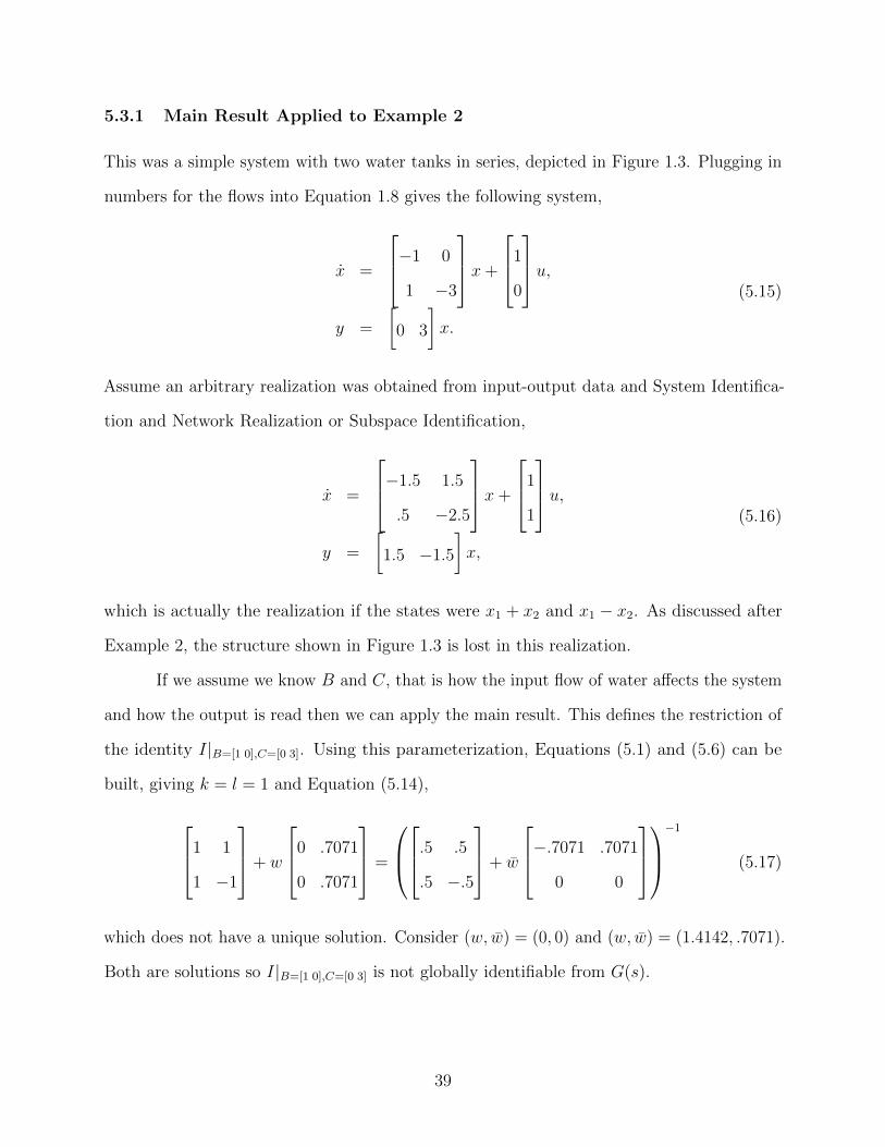
5.3.1 Main Result Applied to Example 2
This was a simple system with two water tanks in series, depicted in Figure 1.3. Plugging in
numbers for the flows into Equation 1.8 gives the following system,
x =
−1 0
1 −3
x+
1
0
u,y =
[0 3
]x.
(5.15)
Assume an arbitrary realization was obtained from input-output data and System Identifica-
tion and Network Realization or Subspace Identification,
x =
−1.5 1.5
.5 −2.5
x+
1
1
u,y =
[1.5 −1.5
]x,
(5.16)
which is actually the realization if the states were x1 + x2 and x1 − x2. As discussed after
Example 2, the structure shown in Figure 1.3 is lost in this realization.
If we assume we know B and C, that is how the input flow of water affects the system
and how the output is read then we can apply the main result. This defines the restriction of
the identity I|B=[1 0],C=[0 3]. Using this parameterization, Equations (5.1) and (5.6) can be
built, giving k = l = 1 and Equation (5.14),
1 1
1 −1
+ w
0 .7071
0 .7071
=
.5 .5
.5 −.5
+ w
−.7071 .7071
0 0
−1
(5.17)
which does not have a unique solution. Consider (w, w) = (0, 0) and (w, w) = (1.4142, .7071).
Both are solutions so I|B=[1 0],C=[0 3] is not globally identifiable from G(s).
39
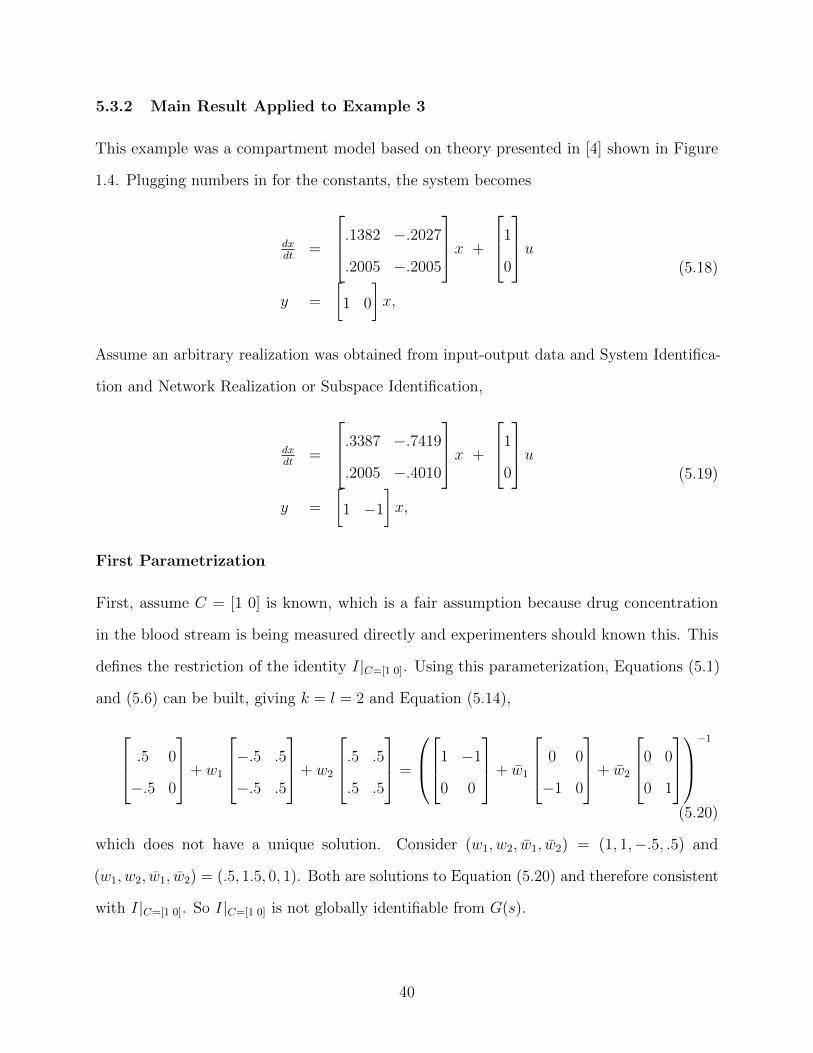
5.3.2 Main Result Applied to Example 3
This example was a compartment model based on theory presented in [4] shown in Figure
1.4. Plugging numbers in for the constants, the system becomes
dxdt
=
.1382 −.2027
.2005 −.2005
x +
1
0
uy =
[1 0
]x,
(5.18)
Assume an arbitrary realization was obtained from input-output data and System Identifica-
tion and Network Realization or Subspace Identification,
dxdt
=
.3387 −.7419
.2005 −.4010
x +
1
0
uy =
[1 −1
]x,
(5.19)
First Parametrization
First, assume C = [1 0] is known, which is a fair assumption because drug concentration
in the blood stream is being measured directly and experimenters should known this. This
defines the restriction of the identity I|C=[1 0]. Using this parameterization, Equations (5.1)
and (5.6) can be built, giving k = l = 2 and Equation (5.14),
.5 0
−.5 0
+ w1
−.5 .5
−.5 .5
+ w2
.5 .5
.5 .5
=
1 −1
0 0
+ w1
0 0
−1 0
+ w2
0 0
0 1
−1
(5.20)
which does not have a unique solution. Consider (w1, w2, w1, w2) = (1, 1,−.5, .5) and
(w1, w2, w1, w2) = (.5, 1.5, 0, 1). Both are solutions to Equation (5.20) and therefore consistent
with I|C=[1 0]. So I|C=[1 0] is not globally identifiable from G(s).
40
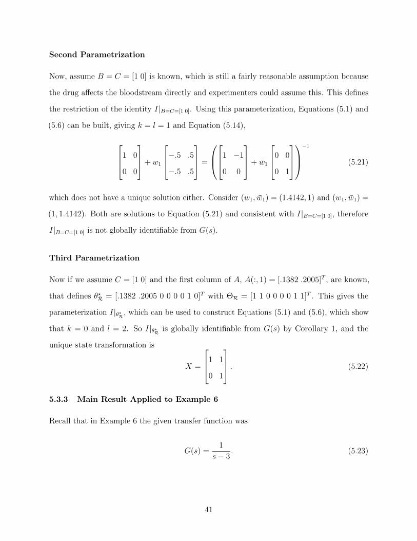
Second Parametrization
Now, assume B = C = [1 0] is known, which is still a fairly reasonable assumption because
the drug affects the bloodstream directly and experimenters could assume this. This defines
the restriction of the identity I|B=C=[1 0]. Using this parameterization, Equations (5.1) and
(5.6) can be built, giving k = l = 1 and Equation (5.14),
1 0
0 0
+ w1
−.5 .5
−.5 .5
=
1 −1
0 0
+ w1
0 0
0 1
−1
(5.21)
which does not have a unique solution either. Consider (w1, w1) = (1.4142, 1) and (w1, w1) =
(1, 1.4142). Both are solutions to Equation (5.21) and consistent with I|B=C=[1 0], therefore
I|B=C=[1 0] is not globally identifiable from G(s).
Third Parametrization
Now if we assume C = [1 0] and the first column of A, A(:, 1) = [.1382 .2005]T , are known,
that defines θ?R = [.1382 .2005 0 0 0 0 1 0]T with ΘR = [1 1 0 0 0 0 1 1]T . This gives the
parameterization I|θ∗R , which can be used to construct Equations (5.1) and (5.6), which show
that k = 0 and l = 2. So I|θ∗R is globally identifiable from G(s) by Corollary 1, and the
unique state transformation is
X =
1 1
0 1
. (5.22)
5.3.3 Main Result Applied to Example 6
Recall that in Example 6 the given transfer function was
G(s) =1
s− 3. (5.23)
41
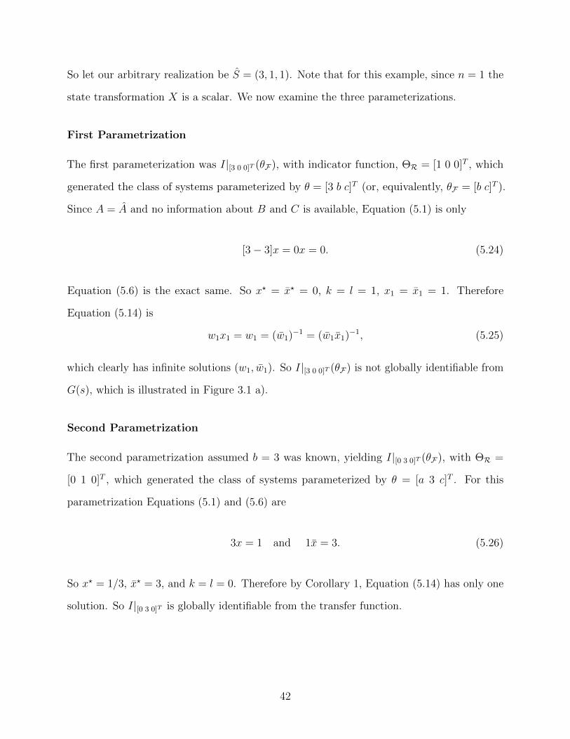
So let our arbitrary realization be S = (3, 1, 1). Note that for this example, since n = 1 the
state transformation X is a scalar. We now examine the three parameterizations.
First Parametrization
The first parameterization was I|[3 0 0]T (θF), with indicator function, ΘR = [1 0 0]T , which
generated the class of systems parameterized by θ = [3 b c]T (or, equivalently, θF = [b c]T ).
Since A = A and no information about B and C is available, Equation (5.1) is only
[3− 3]x = 0x = 0. (5.24)
Equation (5.6) is the exact same. So x? = x? = 0, k = l = 1, x1 = x1 = 1. Therefore
Equation (5.14) is
w1x1 = w1 = (w1)−1 = (w1x1)
−1, (5.25)
which clearly has infinite solutions (w1, w1). So I|[3 0 0]T (θF) is not globally identifiable from
G(s), which is illustrated in Figure 3.1 a).
Second Parametrization
The second parametrization assumed b = 3 was known, yielding I|[0 3 0]T (θF), with ΘR =
[0 1 0]T , which generated the class of systems parameterized by θ = [a 3 c]T . For this
parametrization Equations (5.1) and (5.6) are
3x = 1 and 1x = 3. (5.26)
So x? = 1/3, x? = 3, and k = l = 0. Therefore by Corollary 1, Equation (5.14) has only one
solution. So I|[0 3 0]T is globally identifiable from the transfer function.
42
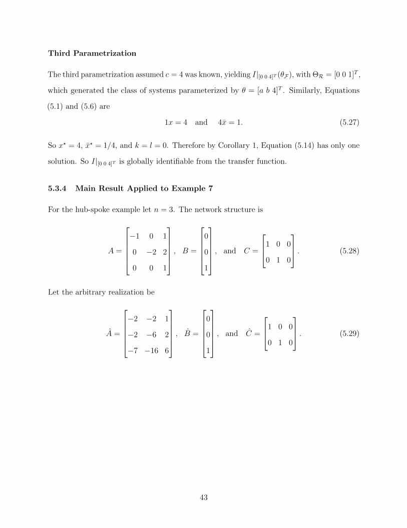
Third Parametrization
The third parametrization assumed c = 4 was known, yielding I|[0 0 4]T (θF), with ΘR = [0 0 1]T ,
which generated the class of systems parameterized by θ = [a b 4]T . Similarly, Equations
(5.1) and (5.6) are
1x = 4 and 4x = 1. (5.27)
So x? = 4, x? = 1/4, and k = l = 0. Therefore by Corollary 1, Equation (5.14) has only one
solution. So I|[0 0 4]T is globally identifiable from the transfer function.
5.3.4 Main Result Applied to Example 7
For the hub-spoke example let n = 3. The network structure is
A =
−1 0 1
0 −2 2
0 0 1
, B =
0
0
1
, and C =
1 0 0
0 1 0
. (5.28)
Let the arbitrary realization be
A =
−2 −2 1
−2 −6 2
−7 −16 6
, B =
0
0
1
, and C =
1 0 0
0 1 0
. (5.29)
43
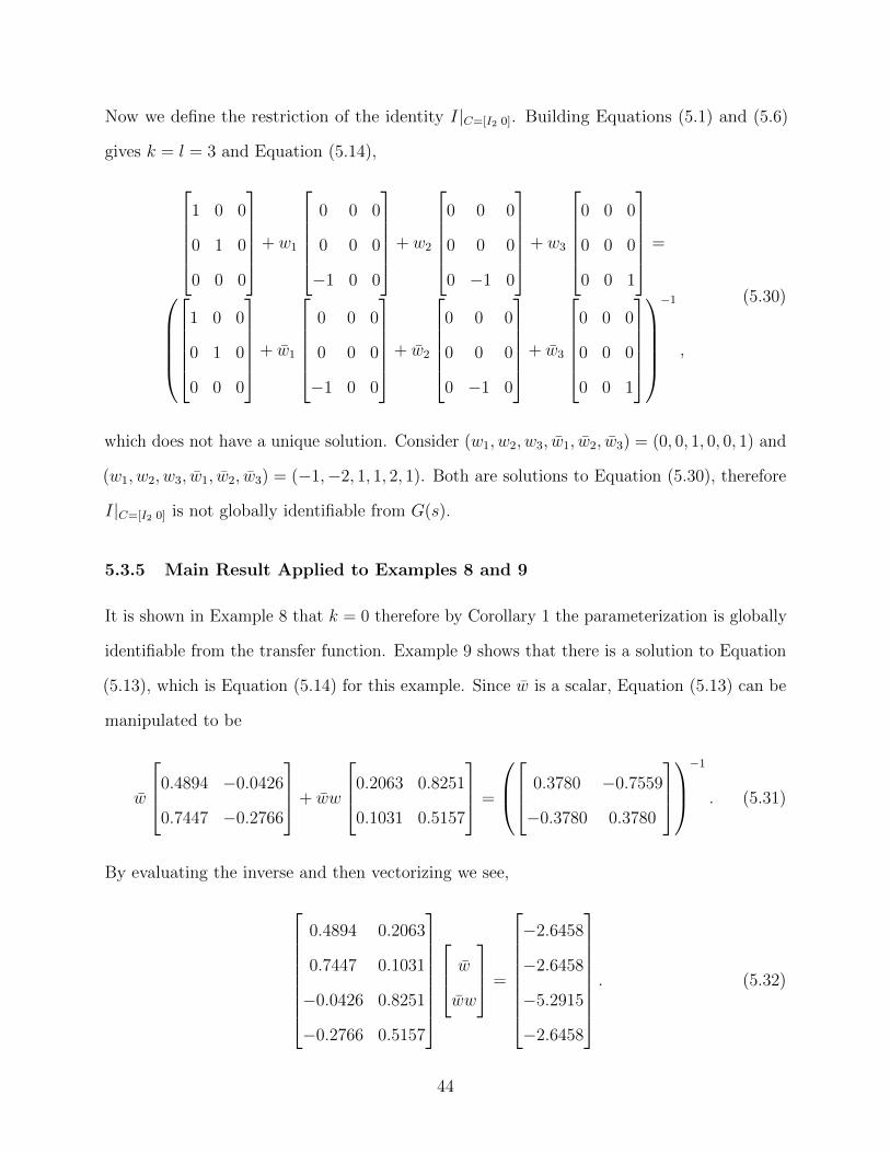
Now we define the restriction of the identity I|C=[I2 0]. Building Equations (5.1) and (5.6)
gives k = l = 3 and Equation (5.14),
1 0 0
0 1 0
0 0 0
+ w1
0 0 0
0 0 0
−1 0 0
+ w2
0 0 0
0 0 0
0 −1 0
+ w3
0 0 0
0 0 0
0 0 1
=
1 0 0
0 1 0
0 0 0
+ w1
0 0 0
0 0 0
−1 0 0
+ w2
0 0 0
0 0 0
0 −1 0
+ w3
0 0 0
0 0 0
0 0 1
−1
,
(5.30)
which does not have a unique solution. Consider (w1, w2, w3, w1, w2, w3) = (0, 0, 1, 0, 0, 1) and
(w1, w2, w3, w1, w2, w3) = (−1,−2, 1, 1, 2, 1). Both are solutions to Equation (5.30), therefore
I|C=[I2 0] is not globally identifiable from G(s).
5.3.5 Main Result Applied to Examples 8 and 9
It is shown in Example 8 that k = 0 therefore by Corollary 1 the parameterization is globally
identifiable from the transfer function. Example 9 shows that there is a solution to Equation
(5.13), which is Equation (5.14) for this example. Since w is a scalar, Equation (5.13) can be
manipulated to be
w
0.4894 −0.0426
0.7447 −0.2766
+ ww
0.2063 0.8251
0.1031 0.5157
=
0.3780 −0.7559
−0.3780 0.3780
−1
. (5.31)
By evaluating the inverse and then vectorizing we see,
0.4894 0.2063
0.7447 0.1031
−0.0426 0.8251
−0.2766 0.5157
w
ww
=
−2.6458
−2.6458
−5.2915
−2.6458
. (5.32)
44
The matrix on the left is full column rank so there is only one solution, which means there is
only one solution to Equation (5.13). Therefore the parameterization is globally identifiable
from G(s), which we saw in Example 9 when we correctly recovered the network structure.
45
Chapter 6
Conclusion
The contribution of this work is the formulation and solution of a new problem in
systems and control theory, called the Network Realization Problem. The problem is, given
a transfer function produced by a set of state-space matrices (A,B,C,D), how many and
which elements of the state-space matrices must be known a priori in order to recover all of
(A,B,C,D). This work was motivated by the desire to completely quantify the conditions
for transitioning between the different mathematical representations of linear time-invariant
systems. The solution to this problem, presented in Theorem 2, is useful for theorists because
it lays a foundation for quantifying the information cost of identifying a system’s complete
network structure from the transfer function. Furthermore it also explains that the value of a
priori information is not necessarily quantified by the amount of information. For example,
knowing the n2 elements of the A matrix is not sufficient but knowing the n2 elements of
the C matrix, if it is invertible, is sufficient (Corollary 2). This is true because a full rank C
matrix completely specifies the states while the A matrix does not.
This problem was also motivated by different prevalent applications that have network
structure as shown in Examples 2-4 and in [6, 28–32]. Practitioners in a variety of applications
will benefit from this work because it will help them understand the kinds of additional
information, beyond input-output data, they must obtain to reconstruct the network structure
of their systems, satisfying a unique solution to Equation (5.14). If this cost is too high or
unattainable, it will motivate them to seek other mathematical models, possibly such as the
DSF [33].
46
6.1 Place in Systems Theory
This work is shown to be related to the key topics in Systems Theory, namely System
Identification, State Realization, Subspace Identification, and Structural Identifiability. The
Network Realization Problem was shown to be a sub-problem of Structural Identifiability
because it deals with identifiability of a specific kind of parameterization and Structural
Identifiability deals with general parameterizations.
The Network Realization Problem was posed as a question of global identifiability from
the transfer function because global identifiability from the transfer function was presented in
[2] and gave a natural home for this problem of trying to recover the network structure. So it
is connected to System Identification because identification produces a transfer function from
input-output data. However nothing in the result required the transfer function, only an
arbitrary realization (A, B, C, D), which we assumed came through State Realization of the
transfer function. This arbitrary realization could come from System Identification followed
by State Realization but since Subspace Identification also produces an arbitrary realization,
it could have come from Subspace Identification. Despite where (A, B, C, D) came from, the
network structure can be recovered if and only if Equation (5.14) has a unique solution.
6.2 Future Work
The necessary and sufficient conditions are provided therefore the problem is solved. However,
as Section 5.2 alludes to, it would be interesting to known exactly when Equation (5.14) has
a unique solution and in so doing quantify the information cost of recovering the network
structure of a system. Another natural question is what are the necessary and sufficient
conditions for obtaining the network structure from other representations of structure such
as dynamical structure functions ([33]) or subsystem structure ([35]). These representations
have more information built into them, such as for dynamical structural functions how the
measured states affect each other, therefore it may be easier to recover the network structure.
47
Chapter 7
References
[1] B. D. Schutter, “Minimal state-space realization in linear system theory: an overview,”
Journal of Computational and Applied Mathematics, vol. 121, no. 1, pp. 331–354, 2000.
[2] K. Glover and J. C. Willems, “Parametrizations of linear dynamical systems: canonical
forms and identifiability,” Automatic Control, IEEE Transactions on, vol. 19, no. 6,
pp. 640–646, 1974.
[3] K. J. Astrom and R. M. Murray, Feedback systems: an introduction for scientists and
engineers. Princeton university press, 2010.
[4] T. Teorell, “Kinetics of distribution of substances administered to the body, i and ii.,”
Archives internationales de pharmacodynamie et de therapie, vol. 57, pp. 205–240, 1937.
[5] G. D. Thomas, M. J. Chappell, P. W. Dykes, D. B. Ramsden, K. R. Godfrey, J. R.
Ellis, and A. R. Bradwell, “Effect of dose, molecular size, affinity, and protein binding
on tumor uptake of antibody or ligand: a biomathematical model,” Cancer research,
vol. 49, no. 12, pp. 3290–3296, 1989.
[6] M. J. Chappell, K. R. Godfrey, and S. Vajda, “Global identifiability of the parameters
of nonlinear systems with specified inputs: a comparison of methods,” Mathematical
Biosciences, vol. 102, no. 1, pp. 41–73, 1990.
[7] L. Ljung, System Identification: Theory for the User. Springer, 1998.
[8] E. G. Gilbert, “Controllability and observability in multivariable control systems,”
Journal of the Society for Industrial & Applied Mathematics, Series A: Control, vol. 1,
no. 2, pp. 128–151, 1963.
[9] R. E. Kalman, “Mathematical description of linear dynamical systems,” Journal of
the Society for Industrial & Applied Mathematics, Series A: Control, vol. 1, no. 2,
pp. 152–192, 1963.
48
[10] B. Ho and R. E. Kalman, “Effective construction of linear state-variable models from
input/output functions,” Proceedings of the 3rd Annual Allerton Conference on Circuit
and System Theory, vol. 1, no. 2, p. 449459, 1965.
[11] B. Ho and R. E. Kalman, “Effective construction of linear state-variable models from
input/output functions,” Regelungstechnik, vol. 14, no. 12, pp. 545–548, 1966.
[12] J. Ackermann and R. S. Bucy, “Canonical minimal realization of a matrix of impulse
response sequences,” Information and Control, vol. 19, no. 3, pp. 224–231, 1971.
[13] L. M. Silverman, “Realization of linear dynamical systems,” Automatic Control, IEEE
Transactions on, vol. 16, no. 6, pp. 554–567, 1971.
[14] S.-Y. Kung, “A new identification and model reduction algorithm via singular value
decomposition,” in Proc. 12th Asilomar Conf. Circuits, Syst. Comput., Pacific Grove,
CA, pp. 705–714, 1978.
[15] J.-N. Juang and R. S. Pappa, “An eigensystem realization algorithm for modal parameter
identification and model reduction,” Journal of guidance, control, and dynamics, vol. 8,
no. 5, pp. 620–627, 1985.
[16] A. M. King, U. B. Desai, and R. E. Skelton, “A generalized approach to q-markov