NECESSARY AND SUFFICIENT CONDITIONS FOR THE POSITIVITY OF SOLUTIONS OF SYSTEMS OF STOCHASTIC PDES by Jacky Cresson 1,2 , Messoud Efendiev 3 & Stefanie Sonner 3 1. Laboratoire de Mathématiques Appliquées de Pau, Université de Pau et des Pays de l’Adour, avenue de l’Université, BP 1155, 64013 Pau Cedex, France 2. Institut de Mécanique Céleste et de Calcul des Éphémérides, Observatoire de Paris, 77 avenue Denfert-Rochereau, 75014 Paris, France 3. Helmholtz Zentrum München, Institut für Biomathematik und Biometrie, Ingolstädter Landstrasse 1, D-85764 Neuher- berg, Germany Abstract.— We derive necessary and sufficient conditions for preserving the positive cone for a class of semi-linear parabolic systems of stochastic partial differential equations. These conditions are valid for both Itô’s and Stratonovich’s interpretation of stochastic differential equations. Contents Introduction .............................................................. 3 1. Additive Versus Multiplicative Noise and Itô’s Versus Stratonovitch’s Interpretation .................................................... 3 2. Positivity and Stochastic Perturbations of Semi-linear Parabolic Systems: The Simplest Case ................................................ 5 3. Main Result ............................................................ 7 Part I. The Deterministic Case - Necessary and Sufficient Conditions for Positivity ............................................................ 10 1. Semi-linear Systems of Parabolic PDEs .................................. 10 2. A Positivity Criterion .................................................... 11 2000 Mathematics Subject Classification.— 60H15, 35K60, 47H07, 37L30, 65M60, 35K57, 92C15, 35B05, 92B99. Key words and phrases.— Necessary and sufficient conditions, Positive cone, Semi-linear parabolic sys- tems, Stochastic PDEs.
Transcript
NECESSARY AND SUFFICIENT CONDITIONS FOR THEPOSITIVITY OF SOLUTIONS OF SYSTEMS OF STOCHASTIC
1. Laboratoire de Mathématiques Appliquées de Pau, Université de Pau et des Pays de l’Adour, avenue de l’Université, BP1155, 64013 Pau Cedex, France
2. Institut de Mécanique Céleste et de Calcul des Éphémérides, Observatoire de Paris, 77 avenue Denfert-Rochereau, 75014Paris, France
3. Helmholtz Zentrum München, Institut für Biomathematik und Biometrie, Ingolstädter Landstrasse 1, D-85764 Neuher-berg, Germany
Abstract. — We derive necessary and sufficient conditions for preserving the positive conefor a class of semi-linear parabolic systems of stochastic partial differential equations. Theseconditions are valid for both Itô’s and Stratonovich’s interpretation of stochastic differentialequations.
POSITIVITY CRITERION FOR SOLUTIONS OF SYSTEMS OF STOCHASTIC PDES 3
INTRODUCTION
In this article we study the qualitative behaviour of solutions of systems of semi-linearparabolic equations under stochastic perturbations, in particular the positivity of solutions andthe validity of comparison principles. Our results are valid for both Itô’s and Stratonovich’sinterpretation (see [6]) of stochastic PDEs.
1. Additive Versus Multiplicative Noise and Itô’s Versus Stratonovitch’s
Interpretation
We first present two simple examples in order to motivate our results. Let us consider thefollowing ordinary differential equation for a real-valued function u : R → R
dudt = 0
u(0) = u0,(1)
where u0 ∈ R. Certainly, this system preserves the positive cone. Indeed, if the initial datasatisfies u0 ≥ 0, then the corresponding solution remains non-negative u(t;u0) = u0 ≥ 0 forall t > 0.
However, if the system is perturbed by an additive noise, that is a white noise modelled bya standard Wiener process Wt, t ≥ 0 on the probability space (Ω,F , P)
du = 0 dt + dWt
u(0) = u0,(2)
the positivity is not preserved by the solutions of the perturbed stochastic system (2).
Proposition 1. — We assume that the initial data satisfies u0 ≥ 0. Then, there exists t∗ > 0
such that the solution u of system (2) becomes negative, that is u(t∗, ω;u0) < 0.
Proof. — First note that in case of an additive noise Itô’s and Stratonovich’s interpretationof the stochastic differential equation (2) lead to the same integral equation (see [6] p.28),namely
u(t) = u(0) +∫ t
0dWs = u(0) + W (t)−W (0) = u(0) + Wt,
where Wt, t ≥ 0 is a standard Wiener process satisfying W (0) = 0.By the law of iterated logarithm holds
almost surely (cf.[5], p.112). This implies that there is an increasing sequence tnn∈N withlimn→∞ tn = ∞ such that
lim infn→∞
Wtn(ω)√2tn log log tn
= −1
almost surely. Consequently, for N0 sufficiently large follows
Wtn(ω) < −12
√2tn log log tn
for all n ≥ N0. This proves that Wtn → −∞ when n tends to infinity, which implies that thesolution u(tn, ω;u0) < 0 if tn is sufficiently large.
Instead of an additive noise let us consider the perturbation of the original system by alinear, multiplicative noise of the form
du = 0 dt + αu dWt
u(0) = u0,(3)
where the constant α ∈ R. In order to simplify computations we first use Stratonovich’sinterpretation of the stochastic differential equation as in this case ordinary chain rule formulasapply under a change of variables. The solution of system (3) is explicitly given by the process
u(t, ω;u0) = u0eαWt(ω).
Hence, independent of the sign of α ∈ R, the solutions of the perturbed system preservepositivity. We claim that, if the stochastic differential equation (3) is interpreted in the senseof Itô, the solutions possess the same property.
Proposition 2. — Independent of the choice of Itô’s or Stratonovich’s interpretation the so-lutions of the stochastic problem (3) preserve positivity.
Proof. — The case of Stratonovich’s interpretation has been considered above. There is an ex-plicit formula relating the integral equations obtained through Itô’s, respectively Stratonovich’sinterpretation. Interpreting the stochastic equation (3) in the sense of Itô
du = 0 dt + αu · dWt,
it is equivalent to the following Stratonovich equation
du = (0− α2
2u)dt + αu dWt,
which can be solved explicitly. Indeed, the transformation v(t, ω) := e−αWt(ω)u(t, ω) leads tothe equation
dv = (−α2
2v)dt,
POSITIVITY CRITERION FOR SOLUTIONS OF SYSTEMS OF STOCHASTIC PDES 5
with initial data v(0) = u0. Its solution is the process v(ω, t) = u0e−α2
2t and consequently,
u(ω, t) = u0e−(α2
2t−αWt(ω)),
which is certainly non-negative if the initial data u0 is non-negative. We conclude that system(3) preserves the positivity of solutions in Itô’s as well as in Stratonovich’s interpretation.
2. Positivity and Stochastic Perturbations of Semi-linear Parabolic Systems:
The Simplest Case
We are interested in stochastic perturbations of systems of semi-linear parabolic equations.Our main result applied to scalar equations resembles the well-known fact, which was illus-trated by our first example: Additive noise destroys the positivity property of solutions whilethe positivity of solutions is preserved under perturbations by a linear, multiplicative noise.
As one of the simplest cases of the class of stochastic PDEs we study in this article we nowdiscuss the stochastic perturbation of a system of two semi-linear reaction-diffusion equations.For the reasons pointed out above we consider perturbations by a linear, multiplicative noise inboth equations. Let O ⊂ Rn, n ∈ N, be a bounded domain, T > 0 and ui : O× [0, T ]×Ω → R,i = 1, 2, be the solutions of the semi-linear initial value problem
du = (a11∆u + a12∆v + f1(u, v))dt + αu dWt
dv = (a21∆u + a22∆v + f2(u, v))dt + βv dWt
u|∂O = 0, v|∂O = 0u|t=0 = u0, v|t=0 = v0,
(4)
where a = (aij)1≤i,j≤2 is a positive definite matrix with real, constant coefficients. Moreover,the constants α, β ∈ R and the function f = (f1, f2) is assumed to be continuously differen-tiable. We interpret the stochastic system in the sense of Stratonovich and apply an analogoustransformation as before. To be more precise, defining the functions u(t, ω) := e−αWt(ω)u(t, ω)
and v(t, ω) := e−βWt(ω)v(t, ω) leads to the following non-autonomous system of random PDEsdudt = a11∆u + a12e
−(α−β)Wt∆v + e−αWtf1(eαWt u, eβWt v)dvdt = a21e
−(β−α)Wt∆u + a22∆v + e−βWtf2(eαWt u, eβWt v).(5)
Random PDEs can be interpreted pathwise and allow to apply deterministic methods. Bya generalization of the positivity criterion for semi-linear systems in [3] to non-autonomousequations (cf. Part I, Section 2 of our article) we conclude that the solutions of system (5)preserve positivity if and only if the coefficients a12 and a21 are zero and the interaction termsF1(u, v) := e−αWtf1(eαWt u, eβWt v) and F2(u, v) := e−βWtf2(eαWt u, eβWt v) satisfy
for u, v ≥ 0. Note that due to the particular form of the transformation this is the case if andonly if the original reaction functions satisfy
f1(0, v) ≥ 0, f2(u, 0) ≥ 0
for u, v ≥ 0.Let us finally discuss the positivity of solutions when the stochastic system (5) is interpreted
in the sense of Itô. In this case the system is equivalent to the system of Stratonovich equationsdu = (a11∆u + a12∆v + f1(u, v)− α2
2 u)dt + αu dWt
dv = (a21∆v + a22∆u + f2(u, v)− β2
2 v)dt + βv dWt.(6)
Analogous transformations as above lead to the following random system for the functions u
and v dudt = a11∆u + a12e
−(α−β)Wt∆v − α2
2 u + e−αWtf1(eαWt u, eβWt v)dvdt = a21e
−(β−α)Wt∆u + a22∆v − β2
2 v + e−βWtf2(eαWt u, eβWt v).(7)
Applying the deterministic positivity criterion we conclude that the positivity of the solutionsof system (7) is preserved if and only if the coefficients a12 and a21 are zero and the interactionfunctions satisfy
F1(0, v) ≥ 0, F2(u, 0) ≥ 0
for u, v ≥ 0. Here, the modified interaction functions are defined by
F1(u, v) := F1(u, v)− α2
2u, F2(u, v) := F2(u, v)− β2
2v.
Hence, due to the linearity of the additional term obtained when using Itô’s interpretationthis condition is satisfied if and only if the functions F1 and F2 fulfil the same property. Thisin turn is equivalent to an analogous condition for the interaction functions f1 and f2 of theunperturbed deterministic system. We summarize our discussion in the following proposition.
Proposition 3. — The solutions of the system of Stratonovich equations (4) as well as thesolutions of the corresponding system obtained through Itô’s interpretation of the stochasticsystem preserve positivity if and only if the solutions of the unperturbed system preserve posi-tivity.
We want to point out the following: The conditions on the interaction functions f1 and f2,which are necessary and sufficient for the positivity of solutions of the unperturbed determin-istic system, are equivalent to analogous conditions for the functions F1 and F2 appearing inthe system of random PDEs in the case of Stratonovich’s interpretation. Moreover, they areequivalent to the same conditions on the functions F1 and F2, which we obtain when inter-preting the stochastic differential equations in the sense of Itô. Hence, in the particular case ofstochastic perturbations by a linear, multiplicative noise the qualitative behaviour of solutions
POSITIVITY CRITERION FOR SOLUTIONS OF SYSTEMS OF STOCHASTIC PDES 7
with respect to positivity is not affected - independent of the choice of Itô’s or Stratonovich’sinterpretation.
As was shown above, this is due to the explicit relation between the equations obtainedthrough Itô’s, respectively Stratonovich’s interpretation, and the particular type of transfor-mation leading to the systems of random PDEs. The necessary and sufficient conditions for thepositivity of solutions of the unperturbed system are invariant under all these transformations.
In order to study the general case, where we cannot apply such a simple transformationleading directly to systems of random PDEs, we consider a Wong-Zakaï-type approximationof the stochastic systems of PDEs. As in [2] we interpret the stochastic system in the senseof Itô. We essentially use the main result of this article, which states that the solutions of theapproximate systems converge in expectation, not to the solution of the original system, butto the solution of a modified one. It turns out that the necessary and sufficient conditionsfor the positivity as well as for the validity of comparison results are invariant under thetransformation relating the original system and the modified system. Moreover, the modifiedsystem is exactly the system we obtain when interpreting the original system in the senseof Stratonovich. Hence, we are not only able to derive necessary and sufficient conditionsfor the positivity and the validity of comparison principles for the solutions of a large classof stochastic PDEs, but also to prove that theses conditions are independent of the choiceof Itô’s, respectively Stratonovich’s, interpretation. That is, the qualitative behaviour ofsolutions regarding positivity and the validity of comparison principles is independent of thechoice of the interpretation for the class of stochastic systems we consider.
3. Main Result
The systems of stochastic PDEs we study are of the following form
dul(x, t) =
(−
m∑i=1
Ali(x, t, D)ui(x, t) + f l(x, t, u(x, t))
)dt +
∞∑i=1
qigli(x, t, u(x, t))dW i
t ,(8)
where x ∈ O, t > 0 for l = 1, . . . ,m. We interpret the stochastic system in the sense of Itô.Here, u = (u1, . . . , um) is a vector-valued function, O ⊂ Rn is a bounded domain and Al
i arelinear elliptic operators of second order. Moreover, we assume W i
t , t ≥ 0i∈N is a family ofindependent standard scalar Wiener processes on the canonical Wiener space (Ω,F , P) anddW i
t denotes the corresponding Ito differential. The boundary conditions are given by theoperators (B1, . . . , Bm),
for l = 1, . . . ,m.We denote by (A, f, g) the previous system (8) of Itô equations and the corresponding
unperturbed deterministic system by (A, f, 0). In our article we will derive necessary andsufficient conditions for the coefficient functions of the operators Al
i and the functions f andg to ensure that system (8) preserves the positivity of solutions. In this case, that is, if thesolutions corresponding to non-negative initial data remain non-negative as long as they exist,we say that the system satisfies the positivity property. The deterministic case has been studiedin [3]. Assuming that the unperturbed deterministic system (A, f, 0) satisfies the positivityproperty we are in particular interested in characterizing the class of stochastic perturbationsg such that the system (A, f, g) satisfies the positivity property.
In the first section of our article, we prove that necessary and sufficient conditions forthe positivity of solutions of the unperturbed system are that the matrices appearing in thedifferential operator A are diagonal and the components of the interaction function satisfy
f l(x, t, u1, . . . , ul−1, 0, ul+1, . . . , un) ≥ 0 for uj ≥ 0 and x ∈ O, t ≥ 0,
where j, l = 1, . . . ,m. This result extends one of the previous results by Efendiev-Sonner (cf.[3]). As a consequence, we are led to the study of the following class of systems with diagonaldifferential operators
for l = 1, . . . ,m, where x ∈ O and t > 0. In the sequel we denote by (f, g) the system ofSPDEs (9) and the corresponding unperturbed system of PDEs by (f, 0).
As mentioned above the main problem we address in this article is the characterizationof stochastic perturbations g such that, if the unperturbed equation satisfies the positivityproperty, then the perturbed stochastic problem (f, g) satisfies also this property. However, weobtain even a stronger result. We derive necessary and sufficient conditions for the interactionfunction f and the stochastic perturbation g such that the system of stochastic Itô PDEs(9) satisfies the positivity property. Moreover, the necessary and sufficient conditions forthe positivity of solutions, as well as for the validity of comparison theorems, are invariantunder the transformation relating the equations obtained through Itô’s and Stratonovich’sinterpretation. As a consequence, our main result is the following:
Theorem 1. — Let (f, g) be a system of stochastic PDEs in Itô or Stratonovich interpreta-tion. We assume that the functions gl
j are twice continuously differentiable with respect to uk,
POSITIVITY CRITERION FOR SOLUTIONS OF SYSTEMS OF STOCHASTIC PDES 9
for all j ∈ N and k, l = 1, . . . ,m. Then, the system (f, g) satisfies the positivity property ifand only if the interaction function f satisfies the deterministic positivity condition and
glj(x, t, u1, . . . , ul−1, 0, ul+1, . . . , um) = 0 (x, t) ∈ O × [0, T ], uk ≥ 0,
for all j ∈ N and k, l = 1, . . . ,m.
The proof makes an essential use of Chueshov-Vuillermot’s result in [2] on a Wong-Zakaïtype approximation theorem for the stochastic problem (f, g). Their main theorem yieldsa smooth random approximation of the stochastic system, which allows to apply determin-istic methods to study the qualitative behaviour of solutions. In particular, we will use ageneralization of the necessary and sufficient conditions for the positivity of solutions in thedeterministic setting obtained by Efendiev-Sonner in [3].
Acknowledgments: We want to thank Tomás Caraballo for helpful discussions.
Our aim is to derive necessary and sufficient conditions for the coefficients of the systemof stochastic partial differential equations (8) to satisfy the positivity property. To this endwe consider a Wong-Zakaï approximation of this system. The approximation preserves thepositivity property of solutions and leads to a family of random equations. To the family ofrandom equations we may apply results from the deterministic theory of PDEs.
Necessary and sufficient conditions for autonomous systems of semi-linear and quasi-linearreaction-diffusion-convection-equations were studied in the article [3]. In the present case,we cannot directly apply these results as the Wong-Zakaï approximation leads to a system ofrandom parabolic equations with time-dependent interaction functions. For the convenienceof the reader we will present a slight generalization of one of the theorems in [3] allowingnon-autonomous interactions functions and arbitrary linear elliptic differential operators ofsecond order. The proof uses the same methods and ideas as applied in the mentioned article.
To be more precise, we consider the following class of systems of semi-linear parabolicequations
∂tul(x, t) = −
m∑i=1
Ali(x,D)ui(x, t) + f l(x, t, u(x, t)),(10)
where u = (u1, . . . , um) is a vector-valued function of x ∈ O, t > 0 and O ⊂ Rn, n ∈ N, is abounded domain with smooth boundary ∂O.
Assumptions on the operator A
The linear second order differential operators Ali(x, D) are defined as
Ali(x,D) = −
n∑k,j=1
ailkj(x)∂xk
∂xj +n∑
k=1
ailk (x)∂xk
,
for i, l = 1, . . . ,m.Comparing with the setting in [2] we omit the zero-order linear terms in the operator A as
for the problems we address it seems more natural to absorb these terms in the interactionfunction f .
POSITIVITY CRITERION FOR SOLUTIONS OF SYSTEMS OF STOCHASTIC PDES 11
We assume that the coefficient functions satisfy ailkj = ail
jk and the operators are uniformlyelliptic, that is
n∑k,j=1
ailkj(x)ζkζj ≥ µ|ζ|2, for all x ∈ O, ζ ∈ Rn,
i, l = 1 . . . , m. Moreover, all coefficient functions are continuously differentiable and boundedin the domain O.
Assumptions on the boundary operators B
The boundary values of the solution are given by the operators
Bl(x,D) = bl0(x) + δl
n∑k=1
blk(x)∂xk
, l = 1, . . . ,m,
where δl ∈ 0, 1. The functions blk, b
l0 are smooth on the boundary ∂O and satisfy bl
0 ≥ 0.Moreover, we assume bl
0 ≡ 1 for δl = 0 and bl = (bl1, . . . , b
lm) is an outward pointing nowhere
tangent vector-field on the boundary ∂O.Assumptions on the non-linear interaction term f
For the (non-linear) interaction function we assume that the partial derivatives ∂uf l exist andare continuous, l = 1, . . . ,m. Moreover, we assume that for x ∈ O and t > 0 the functionsf l = f l(x, t, u) and ∂uf l = ∂uf l(x, t, u) are bounded for bounded values of u.
2. A Positivity Criterion
In order to formulate our criterion for the positivity of solutions we define the positive coneas the set of componentwise almost everywhere non-negative functions.
Definition 1. — By K+ := u : O → Rm | ui ∈ L2(O), ui ≥ 0 a.e. in O, i = 1, . . . ,m wedenote the positive cone, that is the set of all non-negative vector-valued functions on thedomain O.
Our concern is not to study the existence of solutions but their qualitative behaviour. Hence,in the sequel we assume that for any initial data u0 ∈ K+ there exists a unique
solution and for t > 0 the solution satisfies L∞-estimates.The following theorem provides a criterion, which ensures that system (10) satisfies the
positivity property , that is, solutions u( · , · ;u0) : O × [0, T ] → Rm of system (10), whereT > 0, originating from non-negative initial data u0 ∈ K+ remain non-negative (as long asthey exist).
Theorem 2. — Let the operators A and B be defined as in the beginning of this section andthe above conditions on the coefficient functions of the operators and interaction functions besatisfied. Moreover, we assume the initial data u0 ∈ K+ is smooth and fulfils the compatibility
conditions. Then, system (10) satisfies the positivity property if and only if the matrices(ail
kj
)1≤i,l≤m
and(ail
k
)1≤i,l≤m
are diagonal for all 1 ≤ j, k ≤ m and the components of thereaction term satisfy
f i(x, t, u1, . . . , 0︸︷︷︸i
, . . . , um) ≥ 0, for u1 ≥ 0, . . . , um ≥ 0,
1 ≤ i ≤ m, and x ∈ O, t > 0.
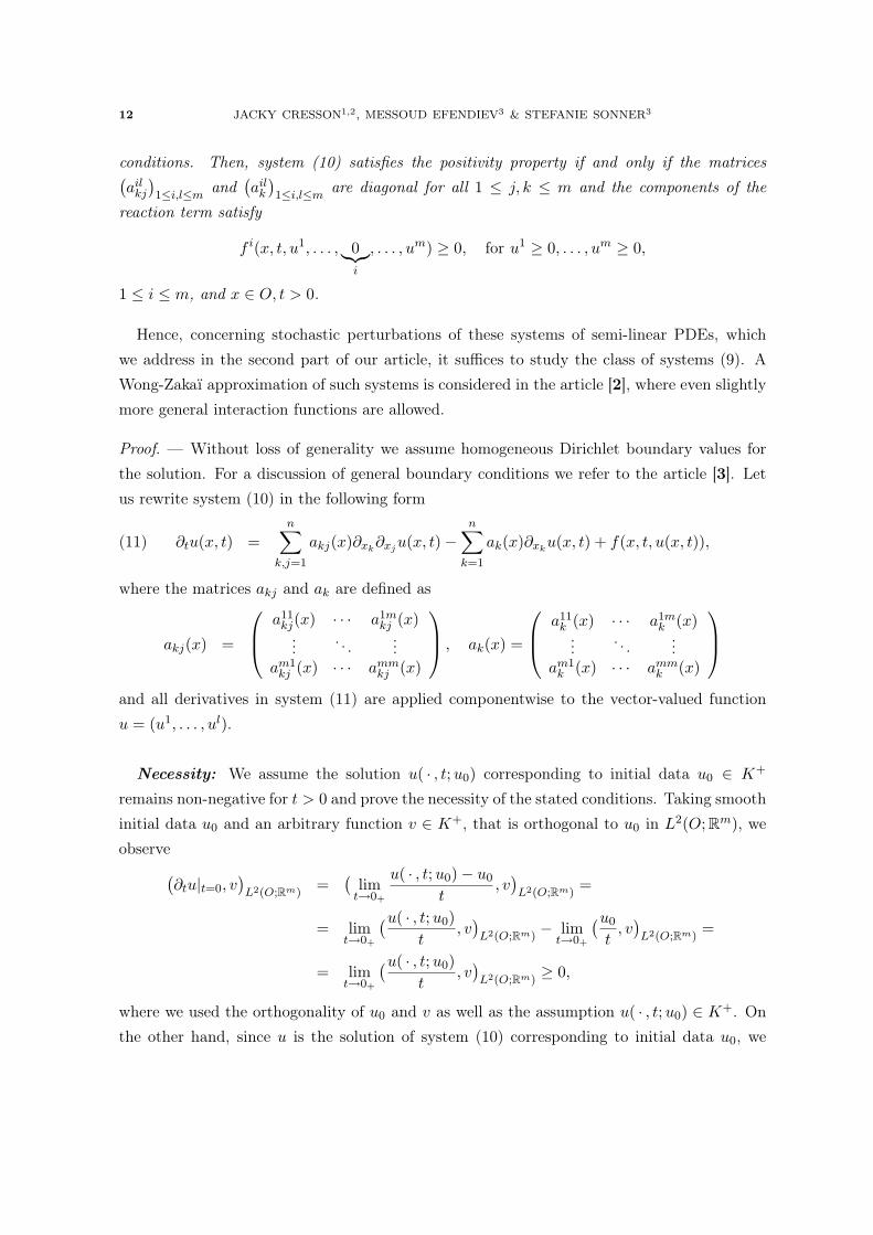
Hence, concerning stochastic perturbations of these systems of semi-linear PDEs, whichwe address in the second part of our article, it suffices to study the class of systems (9). AWong-Zakaï approximation of such systems is considered in the article [2], where even slightlymore general interaction functions are allowed.
Proof. — Without loss of generality we assume homogeneous Dirichlet boundary values forthe solution. For a discussion of general boundary conditions we refer to the article [3]. Letus rewrite system (10) in the following form
∂tu(x, t) =n∑
k,j=1
akj(x)∂xk∂xju(x, t)−
n∑k=1
ak(x)∂xku(x, t) + f(x, t, u(x, t)),(11)
where the matrices akj and ak are defined as
akj(x) =
a11kj(x) · · · a1m
kj (x)...
. . ....
am1kj (x) · · · amm
kj (x)
, ak(x) =
a11k (x) · · · a1m
k (x)...
. . ....
am1k (x) · · · amm
k (x)
and all derivatives in system (11) are applied componentwise to the vector-valued functionu = (u1, . . . , ul).
Necessity: We assume the solution u( · , t;u0) corresponding to initial data u0 ∈ K+
remains non-negative for t > 0 and prove the necessity of the stated conditions. Taking smoothinitial data u0 and an arbitrary function v ∈ K+, that is orthogonal to u0 in L2(O; Rm), weobserve(
∂tu|t=0, v)L2(O;Rm)
=(
limt→0+
u( · , t;u0)− u0
t, v)L2(O;Rm)
=
= limt→0+
(u( · , t;u0)t
, v)L2(O;Rm)
− limt→0+
(u0
t, v)L2(O;Rm)
=
= limt→0+
(u( · , t;u0)t
, v)L2(O;Rm)
≥ 0,
where we used the orthogonality of u0 and v as well as the assumption u( · , t;u0) ∈ K+. Onthe other hand, since u is the solution of system (10) corresponding to initial data u0, we
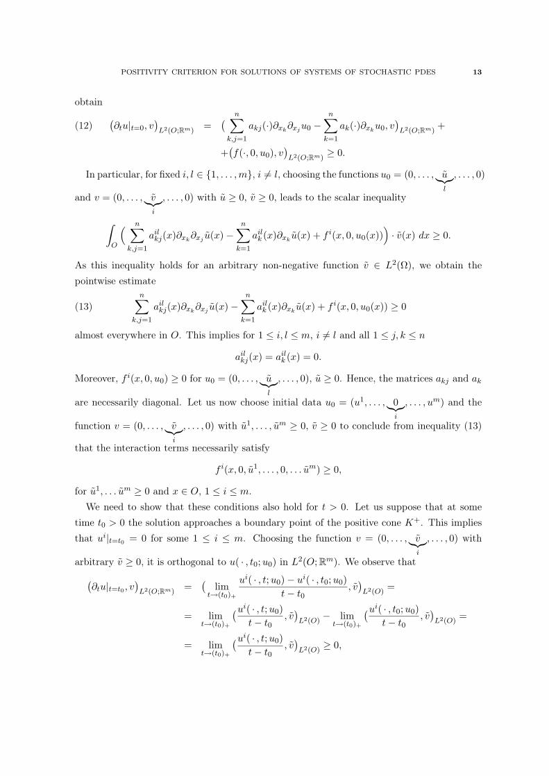
POSITIVITY CRITERION FOR SOLUTIONS OF SYSTEMS OF STOCHASTIC PDES 13
obtain (∂tu|t=0, v
)L2(O;Rm)
=( n∑
k,j=1
akj(·)∂xk∂xju0 −
n∑k=1
ak(·)∂xku0, v
)L2(O;Rm)
+(12)
+(f(·, 0, u0), v
)L2(O;Rm)
≥ 0.
In particular, for fixed i, l ∈ 1, . . . ,m, i 6= l, choosing the functions u0 = (0, . . . , u︸︷︷︸l
, . . . , 0)
and v = (0, . . . , v︸︷︷︸i
, . . . , 0) with u ≥ 0, v ≥ 0, leads to the scalar inequality
∫O
( n∑k,j=1
ailkj(x)∂xk
∂xj u(x)−n∑
k=1
ailk (x)∂xk
u(x) + f i(x, 0, u0(x)))· v(x) dx ≥ 0.
As this inequality holds for an arbitrary non-negative function v ∈ L2(Ω), we obtain thepointwise estimate
n∑k,j=1
ailkj(x)∂xk
∂xj u(x)−n∑
k=1
ailk (x)∂xk
u(x) + f i(x, 0, u0(x)) ≥ 0(13)
almost everywhere in O. This implies for 1 ≤ i, l ≤ m, i 6= l and all 1 ≤ j, k ≤ n
ailkj(x) = ail
k (x) = 0.
Moreover, f i(x, 0, u0) ≥ 0 for u0 = (0, . . . , u︸︷︷︸l
, . . . , 0), u ≥ 0. Hence, the matrices akj and ak
are necessarily diagonal. Let us now choose initial data u0 = (u1, . . . , 0︸︷︷︸i
, . . . , um) and the
function v = (0, . . . , v︸︷︷︸i
, . . . , 0) with u1, . . . , um ≥ 0, v ≥ 0 to conclude from inequality (13)
that the interaction terms necessarily satisfy
f i(x, 0, u1, . . . , 0, . . . um) ≥ 0,
for u1, . . . um ≥ 0 and x ∈ O, 1 ≤ i ≤ m.We need to show that these conditions also hold for t > 0. Let us suppose that at some
time t0 > 0 the solution approaches a boundary point of the positive cone K+. This impliesthat ui|t=t0 = 0 for some 1 ≤ i ≤ m. Choosing the function v = (0, . . . , v︸︷︷︸
i
, . . . , 0) with
arbitrary v ≥ 0, it is orthogonal to u( · , t0;u0) in L2(O; Rm). We observe that(∂tu|t=t0 , v
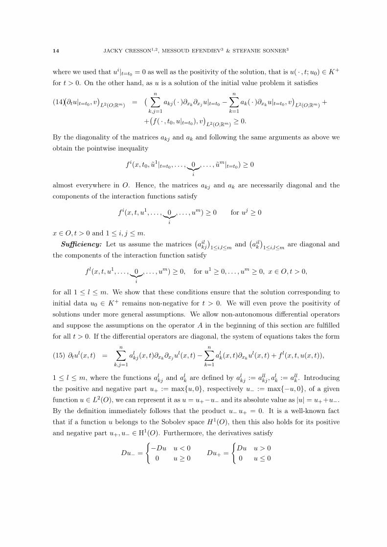
where we used that ui|t=t0 = 0 as well as the positivity of the solution, that is u( · , t;u0) ∈ K+
for t > 0. On the other hand, as u is a solution of the initial value problem it satisfies(∂tu|t=t0 , v
)L2(O;Rm)
=( n∑
k,j=1
akj( · )∂xk∂xju|t=t0 −
n∑k=1
ak( · )∂xku|t=t0 , v
)L2(O;Rm)
+(14)
+(f( · , t0, u|t=t0), v
)L2(O;Rm)
≥ 0.
By the diagonality of the matrices akj and ak and following the same arguments as above weobtain the pointwise inequality
f i(x, t0, u1|t=t0 , . . . , 0︸︷︷︸
i
, . . . , um|t=t0) ≥ 0
almost everywhere in O. Hence, the matrices akj and ak are necessarily diagonal and thecomponents of the interaction functions satisfy
f i(x, t, u1, . . . , 0︸︷︷︸i
, . . . , um) ≥ 0 for uj ≥ 0
x ∈ O, t > 0 and 1 ≤ i, j ≤ m.Sufficiency: Let us assume the matrices
(ail
kj
)1≤i,l≤m
and(ail
k
)1≤i,l≤m
are diagonal andthe components of the interaction function satisfy
f l(x, t, u1, . . . , 0︸︷︷︸i
, . . . , um) ≥ 0, for u1 ≥ 0, . . . , um ≥ 0, x ∈ O, t > 0,
for all 1 ≤ l ≤ m. We show that these conditions ensure that the solution corresponding toinitial data u0 ∈ K+ remains non-negative for t > 0. We will even prove the positivity ofsolutions under more general assumptions. We allow non-autonomous differential operatorsand suppose the assumptions on the operator A in the beginning of this section are fulfilledfor all t > 0. If the differential operators are diagonal, the system of equations takes the form
∂tul(x, t) =
n∑k,j=1
alkj(x, t)∂xk
∂xjul(x, t)−
n∑k=1
alk(x, t)∂xk
ul(x, t) + f l(x, t, u(x, t)),(15)
1 ≤ l ≤ m, where the functions alkj and al
k are defined by alkj := all
kj , alk := all
k . Introducingthe positive and negative part u+ := maxu, 0, respectively u− := max−u, 0, of a givenfunction u ∈ L2(O), we can represent it as u = u+−u− and its absolute value as |u| = u++u−.By the definition immediately follows that the product u− u+ = 0. It is a well-known factthat if a function u belongs to the Sobolev space H1(O), then this also holds for its positiveand negative part u+, u− ∈ H1(O). Furthermore, the derivatives satisfy
Du− =
−Du u < 00 u ≥ 0
Du+ =
Du u > 00 u ≤ 0
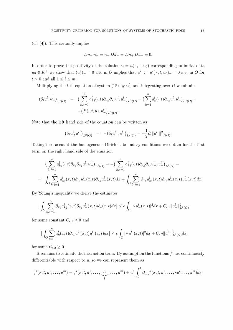
POSITIVITY CRITERION FOR SOLUTIONS OF SYSTEMS OF STOCHASTIC PDES 15
(cf. [4]). This certainly implies
Du+ u− = u+ Du− = Du+ Du− = 0.
In order to prove the positivity of the solution u = u( · , · ;u0) corresponding to initial datau0 ∈ K+ we show that (ui
0)− = 0 a.e. in O implies that ui− := ui( · , t;u0)− = 0 a.e. in O for
t > 0 and all 1 ≤ i ≤ m.Multiplying the l-th equation of system (15) by ul
− and integrating over O we obtain
(∂tu
l, ul−)L2(O)
=( n∑
k,j=1
alkj(·, t)∂xk
∂xjul, ul
−)L2(O)
−( n∑
k=1
alk(·, t)∂xk
ul, ul−)L2(O)
+
+(f l(·, t, u), ul
−)L2(O)
,
Note that the left hand side of the equation can be written as(∂tu
l, ul−)L2(O)
= −(∂tu
l−, ul
−)L2(O)
= −12∂t‖ul
−‖2L2(O).
Taking into account the homogeneous Dirichlet boundary conditions we obtain for the firstterm on the right hand side of the equation
( n∑k,j=1
alkj(·, t)∂xk
∂xjul, ul
−)L2(O)
= −( n∑
k,j=1
alkj(·, t)∂xk
∂xjul−, ul
−)L2(O)
=
=∫
O
n∑k,j=1
alkj(x, t)∂xju
l−(x, t)∂xk
ul−(x, t)dx +
∫O
n∑k,j=1
∂xkal
kj(x, t)∂xjul−(x, t)ul
−(x, t)dx.
By Young’s inequality we derive the estimates
∣∣ ∫O
n∑k,j=1
∂xkal
kj(x, t)∂xjul−(x, t)ul
−(x, t)dx∣∣ ≤ ε
∫O|Oul
−(x, t)|2dx + Cε,1‖ul−‖2
L2(O),
for some constant Cε,1 ≥ 0 and
∣∣ ∫O
n∑k=1
alk(x, t)∂xk
ul−(x, t)ul
−(x, t)dx∣∣ ≤ ε
∫O|Oul
−(x, t)|2dx + Cε,2‖ul−‖2
L2(O)dx,
for some Cε,2 ≥ 0.It remains to estimate the interaction term. By assumption the functions f l are continuously
differentiable with respect to u, so we can represent them as
f l(x, t, u1, . . . , um) = f l(x, t, u1, . . . , 0︸︷︷︸l
that is, f l(x, t, u1, . . . , um) = f l(x, t, u1, . . . , 0, . . . , um)+ul·F l(x, t, u), with a bounded functionF l : Ω× R× Rm → R. This representation yields∫
Of l(x, t, u(x, t)) · ul
−(x, t)dx =∫
Of l(x, t, u1(x, t), . . . , 0︸︷︷︸
l
, . . . , um(x, t)) · ul−(x, t)dx +
+∫
Oul(x, t) · F l(x, t, u(x, t)) · ul
−(x, t)dx =
=∫
Of l(x, t, u1(x, t), . . . , 0︸︷︷︸
l
, . . . , um(x, t)) · ul−(x, t)dx−
∫O|ul−(x, t)|2 · F l(x, t, u(x, t))dx.
Hence, using the uniform parabolicity assumption and collecting all terms we derive the esti-mate
12∂t‖ul
−‖2L2(O) + µ
∫O|Oul
−(x, t)|2dx ≤
≤ 12∂t‖ul
−‖2L2(O) +
∫O
n∑k,j=1
alkj(x, t)∂xju
l−(x, t)∂xk
ul−(x, t)dx ≤
≤∣∣∣ ∫
O
n∑k,j=1
∂xkal
kj(x, t)∂xjul−(x, t)ul
−(x, t)dx +∫
O
n∑k=1
alk(x, t)∂xk
ul−(x, t)ul
−(x, t)dx∣∣∣−
−∫
Of l(x, t, u1(x, t), . . . , 0︸︷︷︸
l
, . . . , um(x, t)) · ul−(x, t)dx +
+∫
O|ul−(x, t)|2 · F l(x, t, u(x, t))dx ≤
≤ 2ε
∫O|Oul
−(x, t)|2dx + (Cε + C)‖ul−‖2
L2(O) −
−∫
O
(f l(x, t, u1(x, t), . . . , 0, . . . , um(x, t))
)ul−(x, t)dx,
for some constants Cε, C ≥ 0. Under the assumption uj ≥ 0, j 6= l, the conditions imposed onthe interaction functions imply
f l(x, t, u1(x, t), . . . , 0︸︷︷︸l
, . . . , um(x, t)) · ul−(x, t) ≥ 0.
Choosing ε > 0 sufficiently small we therefore obtain the inequality
∂t‖ul−‖2
L2(O) ≤ c · ‖ul−‖2
L2(O),
for some constant c ≥ 0. By Gronwall’s Lemma and the initial condition (ul0)− = 0 we
conclude that ul− = 0 a.e. in O for t > 0.
POSITIVITY CRITERION FOR SOLUTIONS OF SYSTEMS OF STOCHASTIC PDES 17
It remains to justify our assumptions on the interaction functions. Instead of the originalsystem (11) we consider the modified system
with F l as defined above. Following the same arguments as before we conclude that thesolution u of this modified system preserves positivity, that is, if the initial data u0 ∈ K+ weobtain u( · , t;u0) ∈ K+ for t > 0. However, the solution u with u1 ≥ 0, . . . , um ≥ 0 satisfiesthe original system
∂tu(x, t) =n∑
k,j=1
akj(x, t)∂xk∂xju(x, t)−
n∑k=1
ak(x, t)∂xku(x, t) + f(x, t, u(x, t))
u|t=0 = u0
u|∂O = 0.
By the uniqueness of the solution corresponding to initial data u0 follows u = u, which impliesthat the solution u of the original system satisfies u( · , t;u0) ∈ K+ for t > 0 and concludesthe proof of the theorem.
Remark 1. — Under appropriate assumptions on the time-dependent coefficients of the op-erator A we could prove an analogous result for non-autonomous differential operators. Asthe proof of the sufficiency of the stated conditions does not change in the non-autonomoussetting we decided to included this generalization in the proof of Theorem 2. The first part ofthe proof however requires some modifications and additional hypothesis. As these questionsare not the main concern of our article we decided to state the theorem in the above form forautonomous differential operators.
CONDITIONS FOR POSITIVITY AND VALIDITY OF COMPARISON
PRINCIPLES
In this section we derive necessary and sufficient conditions for a large class of stochasticsystems of PDEs to satisfy the positivity property. The main ingredient of our proof is aWong-Zakaï-type approximation theorem, which allows us to associate to a given stochasticsystem of PDEs a family of random PDEs. The solutions of the family of random equationsconverge in expectation to the solution of the original problem. As a consequence, we canapply the result for deterministic systems stated in the first part of our article to obtain acriterion for the positivity of solutions of stochastic systems.
1. Wong-Zakaï Approximation and Random Systems of PDEs
In 1965 E. Wong and M. Zakaï ([9],[10]) studied the relation between ordinary and stochas-tic differential equations. The main point is that Itô’s approach to stochastic differential equa-tions is based on Itô’s definition of stochastic integrals, which are not directly connected to thelimit of ordinary integrals. In particular, stochastic differential equations are not defined asan extension or limit of ordinary differential equations. Wong and Zakaï introduce a smoothapproximation of the Brownian motion in order to obtain an approximation of stochasticintegrals by ordinary integrals. Doing so, they obtain an approximation of the stochastic dif-ferential equation by a family of random differential equations. However, when the smoothingparameter tends to zero the random solutions do not converge to a solution of the originalstochastic differential equation, but a modified one. The appearing correction term is calledWong-Zakaï correction term. The Wong-Zakaï approximation theorem has been generalizedin various directions. We refer to D.W. Stroock and S.R.S. Varadhan [7] for systems of ordi-nary differential equations and to G. Tessitore and J. Zabczyk [8] for evolution equations inan abstract setting. In this section, we briefly recall the main result by Chueshov-Vuillermotin [2] about a Wong-Zakaï-type approximation theorem for a class of stochastic systems ofsemi-linear parabolic PDEs.
To be more precise, we will analyse the class of systems of stochastic Itô PDEs (9), wherethe operators in the deterministic part of the equation are defined as in Part I, Section 1.
Assumptions on stochastic perturbations
We assume W jt , t ≥ 0j∈N is a family of mutually independent standard scalar Wiener
POSITIVITY CRITERION FOR SOLUTIONS OF SYSTEMS OF STOCHASTIC PDES 19
processes on the canonical Wiener space (Ω,F , P) and dW jt denotes the corresponding Ito dif-
ferential. The non-negative parameters qj are normalization factors. Moreover, the functionsglj : O × [0, T ] × R → R are smooth and assumed to be bounded for bounded values of the
solution, j ∈ N, l = 1, . . . ,m.
1.1. Smooth Predictable Approximation of the Wiener Process. — A general notionof a smooth predictable approximation of the Wiener process is defined by Chueshov andVuillermot in [2] (Definition 4.1, p.1440). In the following, we will take the main exampleprovided in this article as a definition (Proposition 4.2, p.1441).
Let Wt, t ≥ 0 be a standard scalar Wiener process on the probability space (Ω,F , P)
with filtration Ft; t ∈ R+. The smooth predictable approximation of Wt, t ≥ 0 is thefamily of random processes Wε(t), t ≥ 0ε>0 defined by
Wε(t) =∫ ∞
0φε(t− τ)Wτdτ,
where φε(t) = ε−1φ(t/ε) and φ(t) is a function with the properties
φ ∈ C1(R), suppφ ⊂ [0, 1],∫ 1
0φ(t)dt = 1.
We will need the following result ([2], p.1442), which states that the derivative of the smoothpredictable approximation Wε, denoted by Wε, can be written as a stochastic integral of theform
Wε(t) =∫ t
t−εφε(t− τ)dWτ , t ≥ ε.
As a consequence, Wε is Gaussian, which will be fundamental in our proof.
1.2. Predictable Smoothing of Itô’s Problem and Random Systems. — Using thepreviously defined family of smooth predictable approximations W j
ε (t), t ≥ 0ε>0,j∈N of theWiener processes W j
t , t ≥ 0j∈N allows us to define the predictable smoothing of Itô’s problem(9) as the family of random equations
where l = 1, . . . ,m. As a consequence, using our notation, we are led to the following defini-tion:
Definition 2. — The smooth approximation of the stochastic system (f, g) of PDEswith respect to the smooth predictable approximation Wε(t), t ≥ 0ε>0 is defined as the family
1.3. A Wong-Zakaï Approximation Theorem. — Following Chueshov and Vuillermot([2], p.1436) we use the following notion of mild solution for a stochastic system of PDEs(f, g):
Definition 3. — A random function u(x, t, ω) = (u1(x, t, ω), . . . , um(x, t, ω)) is said to bea mild solution of (f, g) in the space V = W 1
2,B(O, Rm) on the interval [0, T ], if u(t) =
u(x, t, ω) ∈ C(0, T ;L2(Ω×O)) is a predictable process such that∫ T
0E ‖ u(t) ‖2
V dt < ∞
and satisfies the integral equation
(17) u(t) = U(t, 0)u0 +∫ t
0U(t, τ)f(τ, u(τ))dτ +
∞∑j=1
qj
∫ t
0U(t, τ)gj(τ, u(τ))dW j(τ, ω),
where we assume that all integrals in (17) exist.
The family U(t, τ), 0 ≤ τ ≤ t < ∞ in the above definition denotes the linear evolutionfamily generated by the operators A(t), t ≥ 0 in L2(O; Rm). The domain of the linearoperators is defined as
W 22,B(O; Rm) := u ∈ W 2,2(O; Rm) : Bu = 0,
where B denotes the boundary operator and
W 2,2(O) := u ∈ L2(O) : Dαu ∈ L2(O) for all |α| ≤ k.
For further details we refer to [2] and [1]. Next, we introduce the notion of convergence thatwe will use.
Definition 4. — Let (f, g) be a stochastic system of PDEs and (fε,ω, 0) be its smooth approx-imation. We say that a mild solution uε of the random system (fε,ω, 0) converges to a mildsolution u of the stochastic system of PDEs (f , g) if
limε→0
∫ T
0E ‖ u(t)− uε(t) ‖2
W 12 (O;Rm) dt = 0.
The main result of Chueshov and Vuillermot in [2] is the following (Theorem 4.3, p.1443):
POSITIVITY CRITERION FOR SOLUTIONS OF SYSTEMS OF STOCHASTIC PDES 21
Theorem 3. — Assume that the stated assumptions on the operators A and B and the func-tions f and g are satisfied. Moreover, let
∑∞j=1 qj < ∞, the initial data u0 ∈ C2
B(O; Rm) beF0-measurable and E‖u0‖r
C2(O) < ∞ for some r > 8. We assume the associated system ofrandom PDEs (fε,ω, 0) has a mild solution uε belonging to the class C(0, T ;Lr(Ω, Xα,p)) forall 0 ≤ α < 1 and p > 1 and for this solution there exists a constant C independent of ε suchthat
supt∈[0,T ]
E ‖ uε ‖rLp(O)≤ C for all p > 1.
Then, the mild solution uε converges to a solution ucor of the corrected stochastic system ofPDEs (fcor, g) when ε tends to zero, where
f lcor = f l +
12
∞∑j=1
q2j
m∑i=1
gij
∂glj
∂ui,
for l = 1, . . . m.
For further details we refer to the article [2]. Our aim is not to prove the existence ofsolutions, we are interested in their qualitative behaviour. Hence, in the sequel we assumethat a solution of the stochastic initial value problem exists and the solution of the modifiedsystem is given as the limit of the solutions of the smooth random approximations. Sufficientconditions for existence and uniqueness of solutions can be found in the cited article.
2. How to Study the Qualitative Behaviour of Solutions of Systems of Stochastic
PDEs
We will now apply the Wong-Zakaï approximation theorem and the results for the positivityof solutions of deterministic systems in the first part of our article to study the qualitativebehaviour of solutions of systems of stochastic PDEs (f, g).
2.1. The General Strategy. — The general strategy in all proofs is the following:
– As Chueshov and Vuillermot in [2] we associate to a system (F, g) of stochastic PDEs asystem of random PDEs. The system of random PDEs is explicit and depends on thedefinition of the smooth approximation Wε of the Wiener process W (t), t ≥ 0. It isgiven by the family of random PDEs (Fε,ω, 0), ε > 0, ω ∈ Ω, where
F lε,ω = F l +
∞∑j=1
qjgljW
jε ,
for l = 1, . . . ,m, and Wε denotes the time derivative of the smooth predictable approx-imation Wε. The Wong-Zakaï approximation theorem states that the solutions of the
random system of PDEs converge in expectation to the solutions of the modified systemof stochastic PDEs (
F +12
∞∑j=1
q2j hj , g
),
where the function hj = (h1j , . . . , h
mj ) is given by
hlj(x, t, u(x, t)) =
m∑i=1
gij(x, t, u(x, t))
∂glj
∂ui(x, t, u(x, t)).
– Consequently, for a given stochastic system (f, g) we first construct a system of stochasticPDEs (F, g) such that the solutions of its associated system of random PDEs (Fε,ω, 0)
converge to the solutions of our original system (f, g) of stochastic PDEs.– We then use results from the deterministic theory for the qualitative behaviour of solu-
tions of the system of random PDEs (Fε,ω, 0) and prove that this property is preservedby passing to the limit when ε goes to zero.
2.2. An Example: A Comparison Principle and Sufficient Conditions by Chueshov-
Vuillermot. — In this section we present sufficient conditions for the function g to ensurethat, if the solutions of the unperturbed system (f, 0) satisfy a comparison principle, then thisproperty is preserved by the solutions of the perturbed stochastic system.
For two vectors u, v ∈ Rm we write u ≤ v if this order relation holds componentwise, thatis ui ≤ vi for all i = 1, . . . ,m. In order to formulate the result we introduce the followingnotions.
Definition 5. — We say that the deterministic system (f, 0) satisfies the comparison prin-
ciple, if for given initial data such that u0(x) ≤ v0(x) holds a.e. in O the corresponding solu-tions u = (·, ·;u0) and v = v(·, ·; v0) preserve this order relation, that is ui(x, t) ≤ vi(x, t) holdsa.e. in O× [0, T ], for all i = 1, . . . ,m. In an analogous manner the notion of the comparisonprinciple is defined for stochastic systems (f, g).
Furthermore, we call a function f : O× [0, T ]×Rm → Rm quasi-monotone, if it satisfies
f l(x, t, u) ≤ f l(x, t, v)
for all = 1, . . . ,m, (x, t) ∈ O × [0, T ] and all u, v ∈ Rm such that u ≤ v and ul = vl.
The following result is by Chueshov-Vuillermot ([2], Theorem 5.8, p.1479), although weformulate it in a different way in order to adapt it to the notions of our article.
Theorem 4. — Let (f, g) be a system of stochastic PDEs such that the function f is quasi-monotone. We assume that each of the functions gl
j depends on the component ul of thesolution only, that is gl
j(x, t, u) = glj(x, t, ul) for l = 1, . . . ,m, j ∈ N. Then, the stochastic
POSITIVITY CRITERION FOR SOLUTIONS OF SYSTEMS OF STOCHASTIC PDES 23
system (f, g) satisfies the comparison principle.
It is a well-known result in the deterministic theory of PDEs that the quasi-monotonicityof the interaction function f ensures that the system (f, 0) satisfies the comparison principle.Hence, the condition on the functions gl
j stated in the previous theorem is sufficient to ensurethe persistence of this property of the solutions under stochastic perturbations. As mentionedbefore, this theorem was stated in [2]. However, we present a slightly modified proof in orderto illustrate the general strategy outlined in the previous section.
Proof. — Step 1 - Quasi-monotonicity of the associated unperturbed system of
stochastic PDEs
We are looking for a function F such that F + 12
∑∞j=1 q2
j hj = f , where the functions hj
were defined in the previous section. This implies
F l = f l − 12
∞∑j=1
q2j h
lj = f l − 1
2
∞∑j=1
q2j
m∑i=1
gij
∂glj
∂ui= f l − 1
2
∞∑j=1
q2j g
lj
∂glj
∂ul,
l = 1, . . . ,m, j ∈ N, because the functions glj depend on the component ul of the solution
only.Furthermore, f is assumed to be quasi-monotone, that is
f l(x, t, v1, . . . , vl−1, u, vl+1, . . . , vm) ≤ f l(x, t, u1, . . . , ul−1, u, ul+1, . . . , um),
for all (x, t) ∈ O× [0, T ], whenever vk ≤ uk for k = 1, . . . ,m. Due to the assumption that thefunctions gl
j are independent of uk, k 6= l, it therefore follows
f l(x, t, v1, . . . , vl−1, u, vl+1, . . . , vm)− 12
∞∑j=1
q2j g
lj(x, t, u)
∂glj
∂u(x, t, u) ≤
≤ f l(x, t, u1, . . . , ul−1, u, ul+1, . . . , um)− 12
∞∑j=1
q2j g
lj(x, t, u)
∂glj
∂u(x, t, u),
that is, the function F is quasi-monotone as well,
F l(x, t, v1, . . . , vl−1, u, vl+1, . . . , vm) ≤ F l(x, t, u1, . . . , ul−1, u, ul+1, . . . , um),
for vk ≤ uk and all (x, t) ∈ O × [0, T ], l = 1, . . . m.Step 2 - Preservation of quasi-monotonicity by the system of random PDEs
The associated system of random PDEs for (F, g) is given by (Fε,ω, 0), where the function
F lε,ω = F l +
∑∞j=1 qjg
ljW
jε . As the smooth approximations W j
ε of the Wiener process dependonly on the time t and ω ∈ Ω, and the functions gl
F l(x, t, v1, . . . , vl−1, u, vl+1, . . . , vm) +∞∑
j=1
qjglj(x, t, u)W j
ε (t) ≤
≤ F l(x, t, u1, . . . , ul−1, u, ul+1, . . . , um) +∞∑
j=1
qjglj(x, t, u)W j
ε (t),
for all (x, t) ∈ O × [0, T ] and vk ≤ uk, where we used the quasi-monotonicity of the functionF . This is equivalent to
F lε,ω(x, t, v1, . . . , vl−1, u, vl+1, . . . , vm) ≤ F l
ε,ω(x, t, u1, . . . , ul−1, u, ul+1, . . . , um),
for all ε > 0 and ω ∈ Ω. Hence, the property of quasi-monotonicity is preserved by the systemof random PDEs.
To the system of random PDEs (Fε,ω, 0) we may apply the comparison theorem for deter-ministic systems. As a consequence, if the initial data u0 and v0 satisfy u0(x, ω) ≤ v0(x, ω)
for almost all x ∈ O, ω ∈ Ω, we conclude
uε(x, t, ω) ≤ vε(x, t, ω)
for all ε > 0, ω ∈ Ω and almost all (x, t) ∈ O × [0, T ].Step 3 - Passage to the limit when ε goes to zero
By the Wong-Zakaï approximation theorem and our construction of the function F , thesolutions of the system of random PDEs (Fε,ω, 0), ω ∈ Ω, converge in expectation to thesolution of the initial system of stochastic PDEs (f, g). Hence, taking the limit when ε goesto zero, we obtain
u(t, x) ≤ v(t, x), (t, x) ∈ O × [0, T ],
almost surely, which concludes the proof of the theorem.
3. A Positivity Criterion for Systems of Stochastic PDEs
In order to study the positivity of solutions of a given stochastic system (f, g) of PDEswe follow the strategy outlined in Part II, Section 2. For a general stochastic perturbationdetermined by the functions gj = (g1
j , . . . , gmj ), j ∈ N, the associated unperturbed system
(F, 0) of PDEs is given by
F l = f l − 12
∞∑j=1
q2j
(g1j
∂glj
∂u1+ · · ·+ gm
j
∂glj
um
).
In the first part of our article we proved that the deterministic system (f, 0) satisfies thepositivity property if and only if the components f l of the interaction function satisfy
f l(x, t, u1, . . . , ul−1, 0, ul+1, . . . , um) ≥ 0, for all (x, t) ∈ O × [0, T ], uk ≥ 0,(18)
POSITIVITY CRITERION FOR SOLUTIONS OF SYSTEMS OF STOCHASTIC PDES 25
for k, l = 1, . . . ,m. This motivates the following definition.
Definition 6. — We say that the function
f : O × [0, T ]× Rm → Rm, f(x, t, u) = (f1(x, t, u), . . . , fm(x, t, u)),
satisfies the positivity condition if all components f l, 1 ≤ l ≤ m satisfy the property (18).
The following lemma will be essential for the proof of our main result.
Lemma 1. — Let (f, g) be a given stochastic system of PDEs. We assume that the functionsglj are twice continuously differentiable with respect to uk and satisfy
for all j ∈ N and k, l = 1, . . . ,m. Then, the following statements are equivalent:
(a) The function f satisfies the positivity condition.(b) The modified function F satisfies the positivity condition.(c) The associated random functions Fε,ω satisfy the positivity condition for all ε > 0 and
ω ∈ Ω.
Proof. — The proof is a simple computation. As the functions glj are continuously differen-
tiable with respect to ul and glj(x, t, u1, . . . , ul−1, 0, ul+1, . . . , um) = 0 we can represent them
in the form glj(x, t, u) = ulGl
j(x, t, u) with a continuously differentiable function Glj , for all
j ∈ N and l = 1, . . . ,m. Consequently, we obtain for the sum appearing in the Wong-Zakaïcorrection term
m∑i=1
gij
∂glj
∂ui=
m∑i=1
gij
∂(ulGlj)
∂ui=∑i6=l
giju
l∂Gl
j
∂ui+ gl
j
∂(ulGlj)
∂ul,
which leads to an associated function F of the form
F l = f l − 12
∞∑j=1
q2j
m∑i=1
gij
∂glj
∂ui= f l − 1
2
∞∑j=1
q2j
∑i6=l
giju
l∂Gl
j
∂ui+ gl
j
∂(ulGlj)
∂ul
.
Due to the assumption glj(x, t, u1, . . . , ul−1, 0, ul+1, . . . , um) = 0 we note that the function
F satisfies the positivity condition if and only if f satisfies the positivity condition as allcorrection terms vanish when ul = 0. Finally, the associated system of random PDEs (Fε,ω, 0)
is given by
F lε,ω = F l +
∞∑j=1
qjgljW
jε .
The imposed condition on the functions glj therefore implies
where v := (x, t, u1, . . . , ul−1, 0, ul+1, . . . , um), 1 ≤ l ≤ m, which proves that f satisfies thepositivity condition if and only if Fε,ω satisfies the positivity condition and concludes the proofof the lemma.
Applying Lemma 1 we are in position to prove our main result. The following theorem yieldsnecessary and sufficient conditions for the stochastic system (f, g) to satisfy the positivityproperty. In particular, it allows us to characterize the class of stochastic perturbations suchthat the solutions of (f, g) preserve positivity.
Theorem 5. — Let (f, g) be a system of stochastic PDEs. We assume that the functions glj
are twice continuously differentiable with respect to uk, for all j ∈ N and k, l = 1, . . . ,m.Then, the system (f, g) satisfies the positivity property if and only if the interaction functionf satisfies the positivity condition and
glj(x, t, u1, . . . , ul−1, 0, ul+1, . . . , um) = 0 (x, t) ∈ O × [0, T ], uk ≥ 0,
for all j ∈ N and k, l = 1, . . . ,m.
Proof. — Sufficiency: We assume system (f, g) satisfies the stated conditions. In orderto show the positivity of solutions we follow the same strategy as in the proof of Theorem 4.First, associate to the given system (f, g) the unperturbed system of PDEs (F, 0) and considerthe corresponding family of random approximations (Fε,ω, 0). The function g satisfies thehypothesis of Lemma 1 and f the positivity condition, so it follows that the random functionsFε,ω satisfy the positivity condition for all ε > 0 and ω ∈ Ω. The solutions of the randomsystem (Fε,ω, 0) converge in expectation to the solution of the original system (f, g) by Theorem3. Hence, the positivity of the solutions follows exactly as in the proof of Theorem 4.Necessity: We assume the solution of the stochastic system (f, g) remains non-negative fort > 0. In order to show that the stated conditions are necessary we first prove that if
the system (Fε,ω, 0) does not satisfy the positivity property. In fact, if the random system(Fε,ω, 0) satisfies the positivity property, the function Fε,ω necessarily satisfies the positivitycondition. Consequently, for all l = 1, . . . ,m and (x, t) ∈ O × [0, T ] the inequality
F lε,ω(x, t, v) = F l(x, t, v) +
∞∑j=1
qjglj(x, t, v)W j
ε (t) ≥ 0(19)
holds, where v := (u1, . . . , ul−1, 0, ul+1, . . . , um) with u1, . . . , um ≥ 0. The derivative of thesmooth approximation Wε(t) of the Wiener process takes arbitrary values. Hence, if weassume that gl
j(x, t, u1, . . . , ul−1, 0, ul+1, . . . , um) is different from zero, then for sufficientlysmall ε > 0 we always find an ω ∈ Ω such that inequality (19) is violated. Consequently,
POSITIVITY CRITERION FOR SOLUTIONS OF SYSTEMS OF STOCHASTIC PDES 27
the random system (Fε,ω, 0) does not satisfy the positivity property, which contradicts ourassumption and proves that gl
j(x, t, u1, . . . , ul−1, 0, ul+1, . . . , um) = 0 for all j ∈ N, 1 ≤ l ≤ m.Furthermore, if the functions gl
j satisfy this condition, inequality (19) now implies that thefunction F necessarily satisfies the positivity condition. By Lemma 1, this is the case if andonly if the interaction function f of the original system satisfies the positivity condition, whichconcludes the proof of our theorem.
Next, we prove that the same result (see below Corollary 1) is valid if we apply Stratonovich’sinterpretation of stochastic differential equations. In other words, the positivity property ofsolutions is independent of the choice of interpretation, which is the statement of Theorem 1in the introduction.
Corollary 1. — Let (f, g) be a system of stochastic (Itô) PDEs. We assume that the func-tions gl
j are twice continuously differentiable with respect to uk, for all j ∈ N and k, l =
1, . . . ,m. Then, the corresponding system obtained when using Stratonovich’s interpretationof the stochastic system satisfies the positivity property if and only if the functions f and g
satisfy the conditions of the previous theorem.
Proof. — The Wong-Zakaï correction term coincides with the transformation relating Ito’sand Stratonovich’s interpretation of the stochastic system. That is, the solutions of the ran-dom approximations (fε,ω, 0) converge to the solution of the given stochastic system, wheninterpreted in the sense of Stratonovich. Hence, the statement of the corollary is an immediateconsequence of Theorem 5 and Lemma 1.
4. Necessary and Sufficient Conditions for Comparison Principles
As a direct consequence of the positivity criterion we obtain necessary and sufficient con-ditions for the stochastic system to satisfy the comparison principle.
Theorem 6. — Let (f, g) be a system of stochastic PDEs. We assume that the functions glj
are twice continuously differentiable with respect to uk, for all j ∈ N and 1 ≤ k, l ≤ m. Then,the system (f, g) satisfies the comparison principle if and only if the interaction function f isquasi-monotone and the functions gl
j depend on the component ul of the solution only, that is
glj(x, t, u1, . . . , um) = gl
j(x, t, ul)
for all j ∈ N, 1 ≤ l ≤ m.
Proof. — Let u0 and v0 be given initial data satisfying u0(x, ω) ≥ v0(x, ω) for all x ∈ O,ω ∈ Ω.Applying Theorem 5 we derive necessary and sufficient conditions to ensure that the order is
preserved by the corresponding solutions. As the differential operator A is linear, the functionw := u− v is a solution of the stochastic system (f , g) with
f l(x, t, w) := f l(x, t, u)− f l(x, t, v) and glj(x, t, w) := gl
j(x, t, u)− glj(x, t, v)
for j ∈ N, 1 ≤ l ≤ m. Furthermore, by the definition of w the original system (f, g) satisfies thecomparison principle if and only if the system (f , g) satisfies the positivity property. Theorem5 yields necessary and sufficient conditions for the latter. Namely, system (f , g) satisfies thecomparison principle if and only if the function f satisfies the positivity condition and
holds for all j ∈ N and 1 ≤ l ≤ m. The positivity condition for f is equivalent to the quasi-monotonicity of the function f , which proves the stated condition on the interaction function.Moreover, the function g satisfies
holds for all u ∈ R, u ≥ v. This shows that the functions glj depend on the component ul of
the solution only.
Theorem 6 shows that the conditions imposed on the stochastic perturbation g and theinteraction function f by Chueshov and Vuillermot in Theorem 4 are not only sufficient butalso necessary to ensure that the stochastic system satisfies the comparison principle. As inthe case of positivity, the necessary and sufficient conditions for the comparison principle arealso valid, when the stochastic system is interpreted in the sense of Stratonovich.
Corollary 2. — Let (f, g) be a system of stochastic PDEs. We assume that the functionsglj are twice continuously differentiable with respect to uk, for all j ∈ N and 1 ≤ k, l ≤
m. Then, the corresponding system obtained when using Stratonovich’s interpretation of thestochastic system satisfies the comparison principle if and only if the functions f and g satisfythe conditions of the previous theorem.
Proof. — From the proof of Theorem 4 we deduce that, if the stochastic perturbations glj ,
j ∈ N, l = 1, . . . ,m, depend on the component ul of the solution only, then the followingstatements are equivalent:
(a) The function f is quasi-monotone.(b) The modified function F is quasi-monotone.(c) The associated random functions Fε,ω are quasi-monotone for all ε > 0 and ω ∈ Ω.
POSITIVITY CRITERION FOR SOLUTIONS OF SYSTEMS OF STOCHASTIC PDES 29
The solutions of the random approximations (fε,ω, 0) converge to the solution of the givenstochastic system, when interpreted in the sense of Stratonovich. Hence, the statement of thecorollary is an immediate consequence of Theorem 6 and the equivalence relations above.
As in the article [3] a direct consequence of our last theorem are necessary and sufficientconditions for the stochastic system (f, g) to satisfy the comparison principle with respect toan arbitrary order relation in Rm. To be more precise, let σ1 and σ2 be disjoint sets such thatσ1 ∪ σ2 = 1, . . . ,m. For two vectors u and v in Rm we write u v if
uj ≥ vj for j ∈ σ1
uj ≤ vj for j ∈ σ2.
Corollary 3. — Let (f, g) be a system of stochastic PDEs. We assume that the functions glj
are twice continuously differentiable with respect to uk, for all j ∈ N and 1 ≤ k, l ≤ m. Then,the system (f, g) satisfies the comparison principle with respect to the order relation if andonly if the interaction function f satisfies
f l(x, t, u) ≥ f l(x, t, v) l ∈ σ1
f l(x, t, u) ≤ f l(x, t, v) l ∈ σ2,
for x ∈ O, t > 0 and u, v ∈ Rm such that u v and ul = vl, and the functions glj depend on
the component ul of the solution only, that is
glj(x, t, u1, . . . , um) = gl
j(x, t, ul)
for all j ∈ N, 1 ≤ l ≤ m.
Proof. — Let us define the function
wj :=
uj − vj if j ∈ σ1
vj − uj if j ∈ σ2.
Then, the solutions of system (f, g) satisfy the comparison principle with respect to the orderrelation if and only if the function w preserves positivity. By definition, w is a solution ofthe system (f , g) with
f l(x, t, w) :=
f l(x, t, u)− f l(x, t, v) if j ∈ σ1
f l(x, t, v)− f l(x, t, u) if j ∈ σ2
gl(x, t, w) :=
gl(x, t, u)− gl(x, t, v) if j ∈ σ1
gl(x, t, v)− gl(x, t, u) if j ∈ σ2.
As in the proof of Theorem 6 we conclude that system (f , g) satisfies the positivity criterionif and only if the functions gl
j depend on the component ul of the solution only and theinteraction term f satisfies the positivity condition. These conditions are equivalent to theconditions on f and g stated in the theorem.
Remark 2. — The same result is valid when the stochastic system is interpreted in the senseof Stratonovich. This follows exactly as in the case of Theorem 6.
The intuitive interpretation of the conditions we obtained for the stochastic perturbationsis the following. In the critical case, when one component of the solution approaches zero, thestochastic perturbation needs to vanish. Otherwise, the positivity of the solution cannot beguaranteed. As for the validity of comparison principles, the critical situation occurs when thecomponents ul and vl of two given solutions attain the same value. Then, the other componentsof the solution should have no influence on the intensity of the stochastic perturbation andthe stochastic perturbations in the equation for this component of the solution necessarilycoincide.
References
[1] Amann H., Invariant Sets and Existence Theorems for Semilinear Parabolic and Elliptic Systems,Journal of Mathematical Analysis and Applications, No. 65, pp. 432-467, 1978.
[2] Chueshov I.D., Vuillermot P.A., Non-random invariant sets for some systems of Parabolic stochas-tic partial differential equations, Stochastic Analysis and Applications Vol. 22, No. 6, pp. 1421-1486, 2004.
[3] Efendiev M., Sonner S., On verifying mathematical models with diffusion, transport and interac-tion, preprint, 2010.
[4] Gilbarg D., Trudinger N.S., Elliptic Partial Differential Equations of Second Order, 2nd Edition,Springer-Verlag, New York, 1983.
[5] Karatzas I., Shreve S.E., Brownian motion and stochastic calculus, 2d edition, Springer, 1991.[6] Øksendal B., Stochastic Differential Equations: An Introduction with Applications, 6th Edition,
Springer-Verlag, Berlin-Heidelberg, 2003.[7] Stroock D.W., Varadhan S.R.S, On the support of diffusion processes with applications to the
strong maximum principle, Proceedings 6th Berkeley Symposium Math. Statist. Probab., Vol. 3,University of California Press, Berkeley 1972, 333-359.
[8] Tessitore G., Zabczyk J., Wong-Zakai approximations of stochastic evolution equations, J. evol.equ. (2006), 621-655.
[9] Wong E., Zakaï M., On the relationship between ordinary and stochastic differential equations,Internat. J. Engin. Sci. 3 (1965), 213-229.
[10] Wong E., Zakaï M., Riemann-Stieljes approximations of stochastic integrals, Z. Wahrschein-lichkeitstheorie verw. Geb. 12 (1969), 87-97.