Necessary Optimality Conditions for Optimal Control Problems
with Equilibrium Constraints
Lei Guo∗ and Jane J. Ye†
March 2015, revised December 2015, April 2016
Abstract. This paper introduces and studies the optimal control problem with equilib-
rium constraints (OCPEC). The OCPEC is an optimal control problem with a mixed state
and control equilibrium constraint formulated as a complementarity constraint and it can be
seen as a dynamic mathematical program with equilibrium constraints. It provides a powerful
modeling paradigm for many practical problems such as bilevel optimal control problems and
dynamic principal-agent problems. In this paper, we propose weak, Clarke, Mordukhovich
and strong stationarities for the OCPEC. Moreover, we give some sufficient conditions to
ensure that the local minimizers of the OCPEC are Fritz John type weakly stationary, Mor-
dukhovich stationary and strongly stationary, respectively. Unlike Pontryagain’s maximum
principle for the classical optimal control problem with equality and inequality constraints,
a counter example shows that for general OCPECs, there may exist two sets of multipliers
for the complementarity constraints. A condition under which these two sets of multipliers
coincide is given.
Key Words. Optimal control problem with equilibrium constraints, necessary optimality
condition, weak stationarity, Clarke stationarity, Mordukhovich stationarity, strong station-
arity.
2010 Mathematics Subject Classification. 49K15, 49K21, 90C33.
∗Lei Guo, Sino-US Global Logistics Institute, Shanghai Jiao Tong University, Shanghai 200030, China.E-mail: [email protected]. This author’s work was supported in part by NSFC (Grant No. 11401379).†Jane J. Ye, Department of Mathematics and Statistics, University of Victoria, Victoria, BC, V8W 2Y2
Canada. E-mail: [email protected]. This author’s work was supported in part by NSERC.
1
1 Introduction
We are given a time interval [t0, t1] ⊆ IR, a multifunction U mapping [t0, t1] to nonempty
subsets of IRm, and a dynamic function φ : [t0, t1] × IRn × IRm → IRn. A control or control
function u(·) is a measurable function on [t0, t1] such that u(t) ∈ U(t) for almost every
t ∈ [t0, t1]. The state or state trajectory, corresponding to a given control u(·), refers to a
solution x(·) of the following controlled differential equation:
x(t) = φ(t, x(t), u(t)) almost everywhere (a.e.) t ∈ [t0, t1], (1.1)
(x(t0), x(t1)) ∈ E, (1.2)
where E is a given closed subset in IRn × IRn and x(t) is the first-order derivative of the
state x(·) at time t. The differential equation (1.1) linking the state x(·) and the control
u(·) is referred to as the state equation. In optimal control, one looks for a state and control
pair (x(·), u(·)) satisfying the state equation (1.1) and the boundary condition (1.2) so as to
minimize an objective function J(x(·), u(·)). In practice, there are generally extra constraints
to be satisfied by the state and control pair. Such constraints are called mixed state and
control constraints (mixed constraints for short).
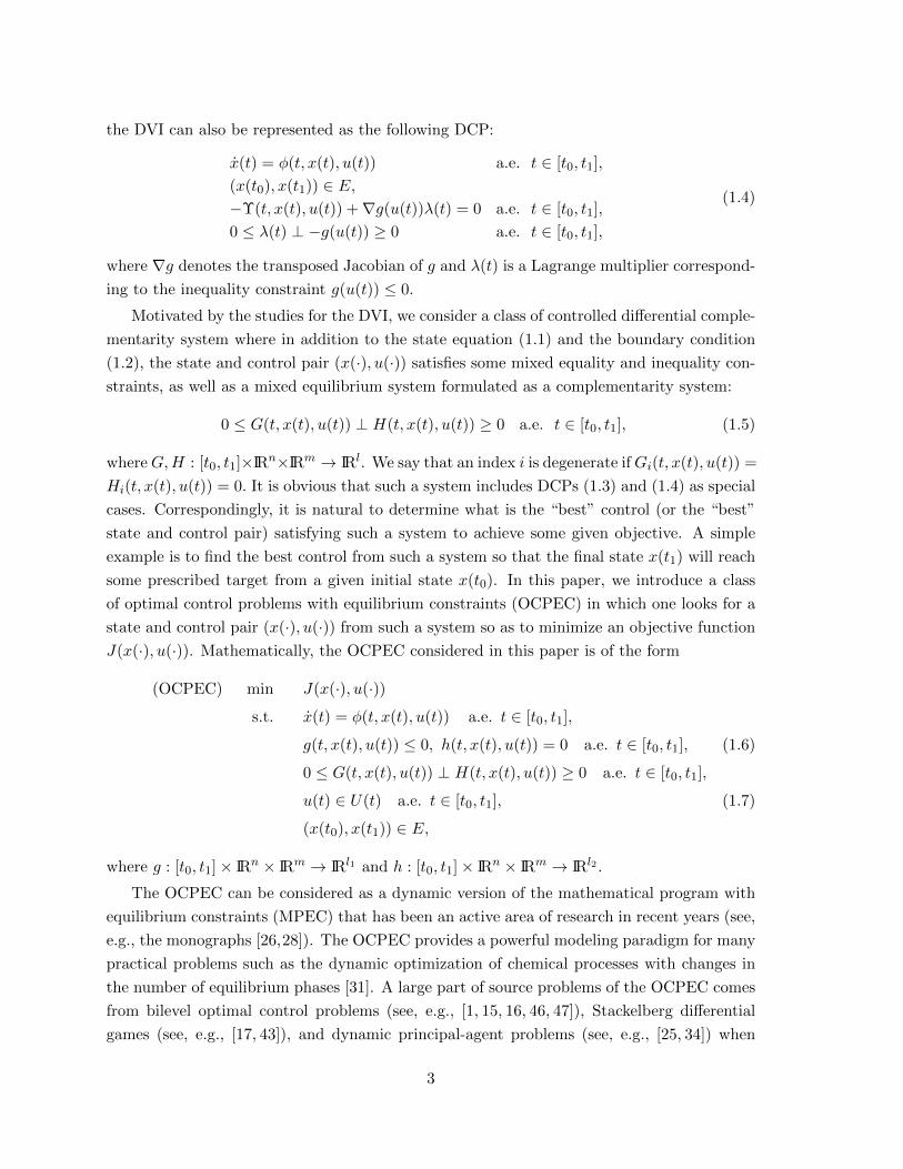
Pang and Stewart [29] recently introduced a class of controlled differential variational
inequality (DVI) problem as follows:
x(t) = φ(t, x(t), u(t)) a.e. t ∈ [t0, t1],
(x(t0), x(t1)) ∈ E,u(t) ∈ K, 〈u′ − u(t),Υ(t, x(t), u(t))〉 ≥ 0 ∀u′ ∈ K a.e. t ∈ [t0, t1],
where Υ : [t0, t1]×IRn×IRm → IRm is a vector-valued function and K is a closed convex subset
in IRm. The DVI provides a powerful modeling paradigm for many practical problems such
as differential Nash equilibrium games ( [4, 29]), multi-rigid-body dynamics with frictional
contacts ( [37]), and hybrid engineering systems ( [18]). In the case where K = IRm+ , the DVI
becomes the controlled differential complementarity problem (DCP)
x(t) = φ(t, x(t), u(t)) a.e. t ∈ [t0, t1],
(x(t0), x(t1)) ∈ E, (1.3)
0 ≤ u(t) ⊥ Υ(t, x(t), u(t)) ≥ 0 a.e. t ∈ [t0, t1],
where a ⊥ b means that vector a is perpendicular to vector b. In the case where K can be
expressed as a set of solutions satisfying some inequality constraints such as
K = u ∈ IRm : g(u) ≤ 0
where g(·) is a convex vector-valued function, when g(·) is affine or Slater’s condition holds,
2
the DVI can also be represented as the following DCP:
x(t) = φ(t, x(t), u(t)) a.e. t ∈ [t0, t1],
(x(t0), x(t1)) ∈ E,−Υ(t, x(t), u(t)) +∇g(u(t))λ(t) = 0 a.e. t ∈ [t0, t1],
0 ≤ λ(t) ⊥ −g(u(t)) ≥ 0 a.e. t ∈ [t0, t1],
(1.4)
where ∇g denotes the transposed Jacobian of g and λ(t) is a Lagrange multiplier correspond-
ing to the inequality constraint g(u(t)) ≤ 0.
Motivated by the studies for the DVI, we consider a class of controlled differential comple-
mentarity system where in addition to the state equation (1.1) and the boundary condition
(1.2), the state and control pair (x(·), u(·)) satisfies some mixed equality and inequality con-
straints, as well as a mixed equilibrium system formulated as a complementarity system:
0 ≤ G(t, x(t), u(t)) ⊥ H(t, x(t), u(t)) ≥ 0 a.e. t ∈ [t0, t1], (1.5)
whereG,H : [t0, t1]×IRn×IRm → IRl. We say that an index i is degenerate ifGi(t, x(t), u(t)) =
Hi(t, x(t), u(t)) = 0. It is obvious that such a system includes DCPs (1.3) and (1.4) as special
cases. Correspondingly, it is natural to determine what is the “best” control (or the “best”
state and control pair) satisfying such a system to achieve some given objective. A simple
example is to find the best control from such a system so that the final state x(t1) will reach
some prescribed target from a given initial state x(t0). In this paper, we introduce a class
of optimal control problems with equilibrium constraints (OCPEC) in which one looks for a
state and control pair (x(·), u(·)) from such a system so as to minimize an objective function
J(x(·), u(·)). Mathematically, the OCPEC considered in this paper is of the form
(OCPEC) min J(x(·), u(·))
s.t. x(t) = φ(t, x(t), u(t)) a.e. t ∈ [t0, t1],
g(t, x(t), u(t)) ≤ 0, h(t, x(t), u(t)) = 0 a.e. t ∈ [t0, t1], (1.6)
0 ≤ G(t, x(t), u(t)) ⊥ H(t, x(t), u(t)) ≥ 0 a.e. t ∈ [t0, t1],
u(t) ∈ U(t) a.e. t ∈ [t0, t1], (1.7)
(x(t0), x(t1)) ∈ E,
where g : [t0, t1]× IRn × IRm → IRl1 and h : [t0, t1]× IRn × IRm → IRl2 .
The OCPEC can be considered as a dynamic version of the mathematical program with
equilibrium constraints (MPEC) that has been an active area of research in recent years (see,
e.g., the monographs [26,28]). The OCPEC provides a powerful modeling paradigm for many
practical problems such as the dynamic optimization of chemical processes with changes in
the number of equilibrium phases [31]. A large part of source problems of the OCPEC comes
from bilevel optimal control problems (see, e.g., [1, 15, 16, 46, 47]), Stackelberg differential
games (see, e.g., [17, 43]), and dynamic principal-agent problems (see, e.g., [25, 34]) when
3
there exist inequality constraints in the lower-level problem. For those problems, if the lower-
level problem, which is a parametric optimal control problem, is replaced by Pontryagain’s
maximum principle (see [30, 38]) which is the well-known first-order necessary optimality
condition for optimal control problems, then an OCPEC results; see, e.g., [15, Section 6.1].
It is desirable to know whether there exists an optimal control before solving the OCPEC.
The Filippov’s existence theorem for Mayer’s problem that is due to Filippov [11] (see also [3,
Theorem 9.2.i]) requires the convexity of the velocity set φ(t, x,U(t, x)) where
U(t, x) := u ∈ U(t) : g(t, x, u) ≤ 0, h(t, x, u) = 0, 0 ≤ G(t, x, u) ⊥ H(t, x, u) ≥ 0.
The velocity set is in general nonconvex due to the existence of the complementarity con-
straints. Thus, the classical existence theorem may not be applicable and one may need
to look for new ways to prove the existence of optimal controls for the OCPEC or use the
existence theorem in a relaxed control setting ( [39,50]). We leave these challenging questions
for future research.
In this paper, we assume that an optimal control exists for the OCPEC and focus on
deriving its necessary optimality conditions. To the best of our knowledge, there is no such
result in the literature so far. Although deriving necessary optimality conditions for optimal
control problems with mixed constraints is a highly challenging problem, some progresses have
been made; see, e.g., [5, 7–10, 20, 21, 24]. Unfortunately, none of these results are applicable
to the OCPEC and its reformulations. The constraint (1.5) is obviously equivalent to that
for almost every t ∈ [t0, t1],
G(t, x(t), u(t)) ≥ 0, H(t, x(t), u(t)) ≥ 0, G(t, x(t), u(t))>H(t, x(t), u(t)) ≤ 0, (1.8)
where > denotes the transpose, which is clearly a system of inequalities. However, all the
inequalities in (1.8) never hold strictly at the same time. This means that the Mangasarian-
Fromovitz constraint qualification (MFCQ) is violated at any point satisfying (1.8). The
classical necessary optimality conditions for optimal control problems with mixed equality
and inequality constraints generally require the linear independence constraint qualification
(LICQ) (see, e.g., [21]) or the Mangasarian-Fromovitz condition (MFC) (see, e.g., [7]) over
some neighborhood of the local minimizer. But both LICQ and MFC are stronger than
MFCQ. Thus, the classical necessary optimality conditions for optimal control problems with
equality and inequality constraints cannot be applied to the OCPEC with the complementar-
ity constraint (1.5) reformulated as inequality constraints (1.8). In the MPEC literature, by
using the so-called “piecewise programming” approach (see, e.g., [26,48]), the feasible region
of an MPEC is locally reformulated as a union of finitely many pieces where each piece is
expressed as a system of equality and inequality constraints, and then it can be shown that
the strong (S-) stationarity holds under the so-called MPEC LICQ. It is obvious that such
an approach fails for the dynamic complementarity system (1.5). A well-known technique to
derive a necessary optimality condition for an MPEC called the Clarke (C-) stationarity is to
4
use the equivalent nonsmooth reformulation minG,H = 0 (“ min ” denotes the componen-
twise minimum) to replace the complementarity system 0 ≤ G ⊥ H ≥ 0 (see, e.g., [35, 45]).
This technique, however, is also not applicable to the OCPEC since such an approach leads to
an optimal control problem with a nonsmooth mixed equality constraint for which there does
not exist any applicable necessary optimality conditions in the control literature. Another
equivalent reformulation of the complementarity constraint is(G,H
)∈ Cl where
Cl := (a, b) ∈ IRl × IRl : 0 ≤ a ⊥ b ≥ 0 (1.9)
is called the complementarity cone. It is known that this reformulation is useful to obtain a
necessary optimality condition in the form of Mordukhovich (M-) stationarity in the MPEC
literature; see, e.g., [45]. Using this reformulation, the OCPEC can be equivalently reformu-
lated as
(Ps) min J(x(·), u(·))
s.t. x(t) = φ(t, x(t), u(t)) a.e. t ∈ [t0, t1], (1.10)
(x(t), u(t)) ∈ S(t) a.e. t ∈ [t0, t1],
(x(t0), x(t1)) ∈ E,
with
S(t) :=
(x, u) ∈ IRn × U(t) :
g(t, x, u) ≤ 0, h(t, x, u) = 0(G(t, x, u), H(t, x, u)
)∈ Cl
. (1.11)
An optimal control problem in the form of (Ps) with an abstract mixed constraint S(t) was
recently studied by Clarke and De Pinho [7]. In this paper, we first derive a slightly sharper
necessary optimality condition for (Ps) than [7, Theorem 2.1] and then apply it to the problem
with S(t) defined as in (1.11). We hope that we would get the M-stationarity as in the MPEC
literature. Unfortunately, for the OCPEC, no sign information on the multipliers associated
with the degenerate indices can be derived and, consequently, we can only obtain a weak
stationarity. In order to get more sign information on the multipliers associated with the
degenerate indices, we further utilize the Weierstrass condition to obtain the second set of
multipliers. A counter example shows that in general these two sets of multipliers may be
different in measure. However, under the MPEC LICQ, since the multipliers corresponding
to the weak stationarity are unique, these two sets of multipliers coincide almost everywhere
and then we can obtain the S-stationarity with one set of multipliers.
The rest of this paper is organized as follows. In Section 2, we give some preliminaries
and preliminary results. In Section 3, we develop the necessary optimality conditions for the
OCPEC. Section 4 illustrates our derived results with a simple example.
5
2 Preliminary and preliminary results
Throughout this paper, ‖ · ‖ denotes the Euclidean norm and Bδ(x) := y : ‖y − x‖ < δthe open ball centered at x with positive radius δ. The boundary, closure, convex hull, and
closed convex hull of a subset Ω ⊆ IRn are denoted by bd Ω, cl Ω, co Ω, and clco Ω, respectively.
Moreover, distΩ(x) denotes the Euclidean distance from x to Ω. For any a, b ∈ IRn, a+ :=
maxa, 0 denotes the nonnegative part of vector a and 〈a, b〉 the inner product of vector a
and vector b. Given a mapping ψ : IRn → IRm and a point x ∈ IRn, ∇ψ(x) stands for the
transposed Jacobian of ψ(·) at x and Iψ(x) := i : ψi(x) = 0 the active index set of ψ(·) at
x. The Minkowski sum of a singleton a and an arbitrary set A is denoted by a + A.
2.1 Background in variational analysis
In this subsection, we review some basic concepts and results in variational analysis that will
be used later on; see, e.g., [6, 27, 33] for more details. Given a subset Ω ⊆ IRn and x ∈ cl Ω,
the proximal normal cone to Ω at x is defined as
NPΩ (x) := v ∈ IRn : ∃ σ ≥ 0 s.t. 〈v, y − x〉 ≤ σ‖y − x‖2 ∀y ∈ Ω,
the limiting normal cone to Ω at x is defined as
NLΩ (x) := v ∈ IRn : ∃(xk, vk)→ (x, v) with vk ∈ NP
Ω (xk) ∀k,
and the Clarke normal cone to Ω at x is defined as NCΩ (x) := clcoNL
Ω (x), which also holds
true even if the space is not finite dimensional but a more general Asplund space [27]. We
can easily obtain the following inclusions:
NPΩ (x) ⊆ NL
Ω (x) ⊆ NCΩ (x) ∀x ∈ cl Ω.
For a multifunction Ξ : IRn ⇒ IRm, its graph and domain are defined, respectively, as
gph Ξ := (x, u) : u ∈ Ξ(x) and dom Ξ := x : Ξ(x) 6= ∅.
Both the limiting normal cone mapping NLΩ (·) and Clarke normal cone mapping NC
Ω (·) are
closed in the sense that their graphs are closed.
The following expression for the limiting normal cone of the complementarity cone Cl is
well-known (see, e.g., [44, Proposition 3.7]) and will be used in Section 3.
Proposition 2.1 For any (a, b) ∈ Cl where Cl is defined in (1.9),
NLCl(a, b) =
(α, β) ∈ IRl × IRl :
αi = 0 if ai > 0, βi = 0 if bi > 0
αi < 0, βi < 0 or αiβi = 0 if ai = bi = 0
.
6
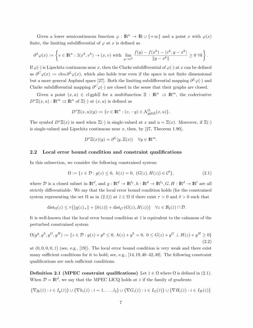
Given a lower semicontinuous function ϕ : IRn → IR ∪ +∞ and a point x with ϕ(x)
finite, the limiting subdifferential of ϕ at x is defined as
∂Lϕ(x) :=
v ∈ IRn : ∃(xk, vk)→ (x, v) with lim
y→xkf(y)− f(xk)− 〈vk, y − xk〉
‖y − xk‖≥ 0 ∀k
.
If ϕ(·) is Lipschitz continuous near x, then the Clarke subdifferential of ϕ(·) at x can be defined
as ∂Cϕ(x) := clco ∂Lϕ(x), which also holds true even if the space is not finite dimensional
but a more general Asplund space [27]. Both the limiting subdifferential mapping ∂Lϕ(·) and
Clarke subdifferential mapping ∂Cϕ(·) are closed in the sense that their graphs are closed.
Given a point (x, u) ∈ cl gphΞ for a multifunction Ξ : IRn ⇒ IRm, the coderivative
D∗Ξ(x, u) : IRm ⇒ IRn of Ξ(·) at (x, u) is defined as
D∗Ξ(x, u)(y) := v ∈ IRn : (v,−y) ∈ NLgphΞ(x, u).
The symbol D∗Ξ(x) is used when Ξ(·) is single-valued at x and u = Ξ(x). Moreover, if Ξ(·)is single-valued and Lipschitz continuous near x, then, by [27, Theorem 1.90],
D∗Ξ(x)(y) = ∂L〈y,Ξ(x)〉 ∀y ∈ IRm.
2.2 Local error bound condition and constraint qualifications
In this subsection, we consider the following constrained system:
Ω := z ∈ D : g(z) ≤ 0, h(z) = 0, (G(z), H(z)) ∈ Cl, (2.1)
where D is a closed subset in IRd, and g : IRd → IRl1 , h : IRd → IRl2 , G,H : IRd → IRl are all
strictly differentiable. We say that the local error bound condition holds (for the constrained
system representing the set Ω as in (2.1)) at z ∈ Ω if there exist τ > 0 and δ > 0 such that
distΩ(z) ≤ τ(‖g(z)+‖+ ‖h(z)‖+ distCl(G(z), H(z))
)∀z ∈ Bδ(z) ∩ D.
It is well-known that the local error bound condition at z is equivalent to the calmness of the
perturbed constrained system
Ω(yg, yh, yG, yH) := z ∈ D : g(z) + yg ≤ 0, h(z) + yh = 0, 0 ≤ G(z) + yG ⊥ H(z) + yH ≥ 0(2.2)
at (0, 0, 0, 0, z) (see, e.g., [19]). The local error bound condition is very weak and there exist
many sufficient conditions for it to hold; see, e.g., [14,19,40–42,49]. The following constraint
qualifications are such sufficient conditions.
Definition 2.1 (MPEC constraint qualifications) Let z ∈ Ω where Ω is defined in (2.1).
When D = IRd, we say that the MPEC LICQ holds at z if the family of gradients
∇gi(z) : i ∈ Ig(z) ∪ ∇hi(z) : i = 1, . . . , l2 ∪ ∇Gi(z) : i ∈ IG(z) ∪ ∇Hi(z) : i ∈ IH(z)
7
is linearly independent.
We say that the MPEC linear condition holds if all the functions g(·), h(·), G(·), H(·) are
affine and D is a union of finitely many polyhedral sets.
We say that the MPEC quasi-normality holds at z if there is no nonzero vector (λ, υ, µ, ν)
such that
• 0 ∈ ∇g(z)λ+∇h(z)υ −∇G(z)µ−∇H(z)ν +NLD (z),
• λ ≥ 0, λi = 0 ∀i /∈ Ig(z), µi = 0 ∀i /∈ IG(z), νi = 0 ∀i /∈ IH(z), µi > 0, νi > 0 or µiνi =
0 ∀i ∈ IG(z) ∩ IH(z),
• there exists a sequence zk ⊆ D converging to z such that for each k,
λi > 0 =⇒ gi(zk) > 0, υi 6= 0 =⇒ υihi(z
k) > 0,
µi 6= 0 =⇒ µiGi(zk) < 0, νi 6= 0 =⇒ νiHi(z
k) < 0.
It should be noted that the MPEC quasi-normality is a weak condition which holds
automatically when the MPEC linear condition holds with D = IRd and is also implied by
the MPEC LICQ.
Proposition 2.2 The local error bound condition holds at z ∈ Ω if the MPEC linear condi-
tion or the MPEC quasi-normality holds at z.
Proof. If the MPEC linear condition holds, then it is easy to see that the perturbed
constrained system Ω(yg, yh, yG, yH) defined in (2.2) is a polyhedral multifunction and hence
the local error bound condition holds [32]. Moreover, by [14, Theorem 5.2], the local error
bound condition follows from the MPEC quasi-normality immediately.
2.3 Optimal control problem with an abstract set constraint
In this subsection, we consider the optimal control problem (Ps) where
J(x(·), u(·)) :=
∫ t1
t0
F (t, x(t), u(t))dt+ f(x(t0), x(t1)).
Here F : [t0, t1]×IRn×IRm → IR and f : IRn×IRn → IR. The basic hypotheses on the problem
data, in force throughout this subsection, are the following: F (·), φ(·) are L×B measurable,
S(·) is L measurable, and f(·) is locally Lipschitz continuous, where L × B denotes the σ-
algebra of subsets of appropriate spaces generated by product sets M × N where M is a
Lebesgue (L) measurable subset in IR and N is a Borel (B) measurable subset in IRn × IRm.
We refer to any absolutely continuous function as an arc. An admissible pair for (Ps) is
a pair of functions (x(·), u(·)) on [t0, t1] for which u(·) is a control and x(·) is an arc that
8
satisfies all the constraints in (Ps). Given a measurable radius function R : [t0, t1]→ (0,+∞],
as in [7], we say that an admissible pair (x∗(·), u∗(·)) is a local minimizer of radius R(·) for
(Ps) if there exists ε > 0 such that for every pair (x(·), u(·)) admissible for (Ps) which also
satisfies
‖x(t)− x∗(t)‖ ≤ ε, ‖u(t)− u∗(t)‖ ≤ R(t) a.e. t ∈ [t0, t1],
∫ t1
t0
‖x(t)− x∗(t)‖ dt ≤ ε,
we have J(x∗(·), u∗(·)) ≤ J(x(·), u(·)). Note that the so-called W 1,1 local minimizer in the
control literature is actually the case where the radius function R(·) is identically +∞.
Let (x∗(·), u∗(·)) be a local minimizer of radius R(·) for (Ps). For every given t ∈ [t0, t1],
a radius function R(·), and a positive constant ε, we define a neighborhood of the point
(x∗(t), u∗(t)) as follows:
Sε,R∗ (t) :=
(x, u) ∈ S(t) : ‖x− x∗(t)‖ ≤ ε, ‖u− u∗(t)‖ ≤ R(t). (2.3)
Other than the basic hypotheses on the problem data, we also assume that the following
assumptions hold for (Ps).
Assumption 2.1 (i) There exist measurable functions kφx(·), kFx (·), kφu(·), kFu (·) such that for
almost every t ∈ [t0, t1] and for every (x1, u1), (x2, u2) ∈ Sε,R∗ (t), we have
‖φ(t, x1, u1)− φ(t, x2, u2)‖ ≤ kφx(t)‖x1 − x2‖+ kφu(t)‖u1 − u2‖,
|F (t, x1, u1)− F (t, x2, u2)| ≤ kFx (t)‖x1 − x2‖+ kFu (t)‖u1 − u2‖.
(ii) There exists a positive measurable function kS(·) such that for almost every t ∈ [t0, t1],
the bounded slope condition holds:
(x, u) ∈ Sε,R∗ (t), (α, β) ∈ NPS(t)(x, u) =⇒ ‖α‖ ≤ kS(t)‖β‖. (2.4)
(iii) The functions kφx(·), kFx (·), kS(·)[kφu(·)+kFu (·)] are integrable and there exists a positive
number η such that R(t) ≥ ηkS(t) a.e. t ∈ [t0, t1].
Assumption 2.1(i) can be seen as a local Lipschitz condition in variable (x, u) with mea-
surable Lipschitz constants. This condition is automatically satisfied with time independent
Lipschitz constants when u∗(·) is bounded over [t0, t1], the radius function R(·) is a positive
constant function, and the functions F (·), φ(·) are locally Lipschitz continuous in variable
(t, x, u). Assumption 2.1(ii) is a key condition proposed in [7] to derive the necessary opti-
mality conditions. We will investigate some sufficient conditions for such an assumption to
hold in our problem setting in Section 3.
For a general optimal differential inclusion problem
min f(x(t0), x(t1))
s.t. x(t) ∈ Ft(x(t)) a.e. [t0, t1],
(x(a), x(b)) ∈ E,
9
where Ft : IRn ⇒ IRn is a multifunction, Clarke [5] has derived a new state of the art
necessary optimality conditions in the optimal control literature. These conditions are strat-
ified in that both the hypotheses and the conclusions are formulated relative to a given
radius function. However, it should be noted that for a point v lying on the boundary
of Ft(x∗(t)) ∩ clBR(t)(u
∗(t)), one may not find a sequence vk in Ft(x∗(t)) ∩ BR(t)(u
∗(t))
such that vk → v if Ft(x∗(t)) is disconnected. Thus, the derived Weierstrass condition
in [5, Theorems 2.3.3 and 3.1.1, and Corollary 3.5.3] should hold only relative to the open
ball BR(t)(u∗(t)) instead of the closed ball clBR(t)(u
∗(t)). In a recent paper [2], Bettiol et al.
also proved the stratified necessary optimality conditions for an optimal differential inclusion
problem involving additional pathwise state constraints in [2, Theorem 2.1] and pointed out
that the Weierstrass condition may not hold with full radius by a counter example [2, Example
2]. Recently, Clarke and De Pinho [7, Theorem 2.1] derived the stratified necessary optimal-
ity conditions for (Ps) by recasting the problem as an equivalent optimal different inclusion
problem and applying the corresponding necessary optimality conditions from [5, Corollary
3.5.3]. In the following, using the same proof technique as in [7, Theorem 2.1], we give a
stratified necessary optimality condition for (Ps) which will be used in obtaining our main
results. Our results differ from [7, Theorem 2.1] in two aspects. Firstly, our Euler inclusion
(c) is slightly sharper than that in [7, Theorem 2.1]. Secondly, the Weierstrass condition (d)
holds only on the open ball BR(t)(u∗(t)) instead of the closed ball clBR(t)(u
∗(t)).
Theorem 2.1 Let (x∗(·), u∗(·)) be a local minimizer of radius R(·) for (Ps) and Assumption
2.1 hold. Then there exist a number λ0 ∈ 0, 1 and an arc p(·) such that
(a) the nontriviality condition holds: (λ0, p(t)) 6= 0 ∀t ∈ [t0, t1];
(b) the transversality condition holds:
(p(t0),−p(t1)) ∈ λ0∂Lf(x∗(t0), x∗(t1)) +NL
E (x∗(t0), x∗(t1));
(c) the Euler inclusion holds: For almost every t ∈ [t0, t1],
(p(t), 0) ∈ co
(w, 0) : (w, 0) ∈ ∂L〈−p(t), φ(t, ·, ·)〉+ λ0F (t, ·, ·)
(x∗(t), u∗(t))
+NLS(t)(x
∗(t), u∗(t))
; (2.5)
(d) the Weierstrass condition holds: For almost every t ∈ [t0, t1],
(x∗(t), u) ∈ S(t), ‖u− u∗(t)‖ < R(t) =⇒〈p(t), φ(t, x∗(t), u)〉 − λ0F (t, x∗(t), u) ≤ 〈p(t), φ(t, x∗(t), u∗(t))〉 − λ0F (t, x∗(t), u∗(t)).
Proof. First we consider the case where F (·) ≡ 0. Similarly as in the proof of [7, Theorem
2.1], for any M > 1, by applying [5, Corollary 3.5.3] with the Weirestrass condition on a open
10
ball BR(t)(u∗(t)) or [2, Theorem 2.1], we can obtain a number λ0,M ∈ 0, 1 and an arc pM (·)
such that the nontriviality condition holds:
λ0,M + ‖pM (·)‖∞ = 1;
the transversality condition holds:
(pM (t0),−pM (t1)) ∈ λ0,M∂Lf(x∗(t0), x∗(t1)) +NL
E (x∗(t0), x∗(t1));
the Euler inclusion holds: For almost every t ∈ [t0, t1],
(pM (t), 0) ∈ co
(w, 0) : (w, pM (t), 0) ∈ NLG(t)(x
∗(t), φ(t, x∗(t), u∗(t)), 0),
where
G(t) :=
(x, φ(t, x, u), c(t)(u− u∗(t))) : (x, u) ∈ S(t)
with c(t) := M(kφx(t) + kS(t)kφu(t))/kS(t); and the Weierstrass condition holds with radius
R(·)M/(M + 1): For almost every t ∈ [t0, t1],
(x∗(t), u) ∈ S(t), ‖u− u∗(t)‖ < R(t)M/(M + 1)
=⇒ 〈pM (t), φ(t, x∗(t), u)〉 ≤ 〈pM (t), φ(t, x∗(t), u∗(t))〉. (2.6)
As shown in [7, Theorem 2.1], we can extract a convergent subsequence of the sequence
(λ0,M , pM (·))M with limit (λ0, p(·)) as M → ∞. Taking limits as M → ∞ in the above
nontriviality condition, transversality condition, Weierstrass condition, and Euler inclusion,
we can obtain the results (a), (b), and (d) of this theorem for the case where F (·) ≡ 0 and
(p(t), 0) ∈ co
(w, 0) : (w, p(t), 0) ∈ NLG(t)(x
∗(t), φ(t, x∗(t), u∗(t)), 0).
The Euler inclusion (c) of this theorem for the case where F (·) ≡ 0 can be obtained by
estimating the limiting normal cone of the above formula as in the last paragraph of Page
4521 in [7].
The general case in which a nonzero F is present is reducible to the already treated one
by augmentation as explained at the end of the proof of [7, Theorem 2.1].
Note that in the proof of Theorem 2.1, we are unable to prove that the Weierstrass
condition holds with full radius R(·) as claimed in the proof of [7, Theorem 2.1]. The reason
is that for a given u lying on the boundary of the set
Ω := u : (x∗(t), u) ∈ S(t), ‖u− u∗(t)‖ ≤ R(t),
to show that
〈p(t), φ(t, x∗(t), u)〉 ≤ 〈p(t), φ(t, x∗(t), u∗(t))〉 (2.7)
in the case where F (·) ≡ 0, we would need to find uM ∈ u : (x∗(t), u) ∈ S(t), ‖u− u∗(t)‖ <R(t)M/(M + 1) such that uM → u as M →∞ and take limits in (2.6) to derive the desired
inequality (2.7). But this may not be always possible if Ω is disconnected.
11
Remark 2.1 Theorem 2.1 is a Fritz John (FJ) type necessary optimality condition. In the
case where λ0 = 0, no information on the objective functions can be derived from the necessary
optimality condition and it becomes useless. Thus, the case where λ0 = 1 is desirable. It
follows from Theorem 2.1 that if there is no nonzero abnormal multiplier, i.e., the following
implication holds:
(p(t0),−p(t1)) ∈ NLE (x∗(t0), x∗(t1)),
(p(t), 0) ∈ co
(w, 0) : (w, 0) ∈ ∂L〈−p(t), φ(t, ·, ·)〉(x∗(t), u∗(t))+NL
S(t)(x∗(t), u∗(t))
a.e. t ∈ [t0, t1],
(x∗(t), u) ∈ S(t), ‖u− u∗(t))‖ < R(t)
=⇒ 〈p(t), φ(t, x∗(t), u)〉 ≤ 〈p(t), φ(t, x∗(t), u∗(t))〉 a.e. t ∈ [t0, t1],
=⇒ p(t) = 0 for some t ∈ [t0, t1],
then the conclusions of Theorem 2.1 hold with λ0 = 1. Such a condition is automatically
satisfied in the case of free initial or final point, that is, E = E0 × IRn or E = IRn × E1
with closed subsets E0, E1 in IRn. Supposing λ0 = 0, the result (b) in Theorem 2.1 yields
that p(t1) = 0 or p(t0) = 0, respectively, which contradicts the result (a) of this theorem.
Throughout the paper, all the derived necessary optimality conditions are FJ type conditions.
The desired case where λ0 = 1 can be obtained provided that there is no nonzero abnormal
multiplier, which is always true if the initial or final point is free.
3 Necessary optimality conditions for OCPEC
In this section, we develop necessary optimality conditions for the OCPEC under the following
basic hypothesises.
Assumption 3.1 (Basic assumption) F : [t0, t1]× IRn× IRm → IR and φ : [t0, t1]× IRn×IRm → IRn are L×B measurable, g : [t0, t1]× IRn× IRm → IRl1 , h : [t0, t1]× IRn× IRm → IRl2,
and G,H : [t0, t1] × IRn × IRm → IRl are L measurable in variable t and strict differentiable
in variable (x, u), U : [t0, t1] ⇒ IRm is a L measurable multifunction, f : IRn × IRn → IR is
locally Lipschitz continuous, and E is a closed subset in IRn × IRn.
In fact, we can easily extend our results to the case where the mappings g(·), h(·), G(·), H(·)are only Lipschitz continuous in variable (x, u) and strictly differentiable at (x∗(t), u∗(t)). But
for simplicity of exposition, we assume that they are strictly differentiable in variable (x, u)
as in Assumption 3.1.
12
Given an admissible pair (x(·), u(·)) and a point t ∈ [t0, t1], we define the index sets:
I−t (x, u) := i : gi(t, x(t), u(t)) < 0,
I0t (x, u) := i : gi(t, x(t), u(t)) = 0,
I+0t (x, u) := i : Gi(t, x(t), u(t)) > 0 = Hi(t, x(t), u(t)),
I00t (x, u) := i : Gi(t, x(t), u(t)) = 0 = Hi(t, x(t), u(t)),
I0+t (x, u) := i : Gi(t, x(t), u(t)) = 0 < Hi(t, x(t), u(t)).
Moreover, for any (λ, υ, µ, ν) ∈ IRl1 × IRl2 × IRl × IRl, we denote
Ψ(t, x, u;λ, υ, µ, ν) := g(t, x, u)>λ+ h(t, x, u)>υ −G(t, x, u)>µ−H(t, x, u)>ν.
Theorem 3.1 Let (x∗(·), u∗(·)) be a local minimizer of radius R(·) for the OCPEC and
Assumption 3.1 hold. Suppose that Assumption 2.1 with S(t) defined in (1.11) is also satisfied.
If for almost every t ∈ [t0, t1], the local error bound condition for the system representing S(t)
as in (1.11) holds at (x∗(t), u∗(t)), then there exist a number λ0 ∈ 0, 1, an arc p(·), and
measurable functions λg : IR→ IRl1 , λh : IR→ IRl2 , λG : IR→ IRl, λH : IR→ IRl such that the
following conditions hold:
(i) the nontriviality condition (λ0, p(t)) 6= 0 ∀t ∈ [t0, t1];
(ii) the transversality condition
(p(t0),−p(t1)) ∈ λ0∂Lf(x∗(t0), x∗(t1)) +NL
E (x∗(t0), x∗(t1));
(iii) the Euler adjoint inclusion: For almost every t ∈ [t0, t1],
(p(t), 0) ∈ ∂C〈−p(t), φ(t, ·, ·)〉+ λ0F (t, ·, ·)
(x∗(t), u∗(t)) + 0 × NC
U(t)(u∗(t))
+∇x,uΨ(t, x∗(t), u∗(t);λg(t), λh(t), λG(t), λH(t)),
λg(t) ≥ 0, λgi (t) = 0 ∀i ∈ I−t (x∗, u∗),
λGi (t) = 0 ∀i ∈ I+0t (x∗, u∗), λHi (t) = 0 ∀i ∈ I0+
t (x∗, u∗);
(iv) the Weierstrass condition for radius R(·): For almost every t ∈ [t0, t1],
(x∗(t), u) ∈ S(t), ‖u− u∗(t)‖ < R(t) =⇒〈p(t), φ(t, x∗(t), u)〉 − λ0F (t, x∗(t), u) ≤ 〈p(t), φ(t, x∗(t), u∗(t))〉 − λ0F (t, x∗(t), u∗(t)).
Proof. For simplicity in the proof, we omit the equality and inequality constraints (1.6),
and the control constraint (1.7) since we have checked that all the formulas of the proof
have the corresponding counterparts when using S(t) defined in (1.11) instead of (3.1). Then
(x∗(·), u∗(·)) is a local minimizer of radius R(·) for (Ps) with S(t) defined as follows:
S(t) =
(x, u) :(G(t, x, u), H(t, x, u)
)∈ Cl
. (3.1)
13
By virtue of Theorem 2.1, we can easily get the results (i), (ii), and (iv) in this theorem. It
now suffices to show the result (iii) by Theorem 2.1(c). Since the local error bound condition
holds at (x∗(t), u∗(t)) and the functions G(t, ·, ·), H(t, ·, ·) are strictly differentiable, it follows
from Proposition 2.1 and [22, Proposition 3.4] that
NLS(t)(x
∗(t), u∗(t))
⊆−∇x,uG(t, x∗(t), u∗(t))β −∇x,uH(t, x∗(t), u∗(t))γ : (β, γ) ∈M∗(t)
, (3.2)
where
M∗(t) :=
(β, γ) :
βi = 0 if i ∈ I+0t (x∗, u∗)
γi = 0 if i ∈ I0+t (x∗, u∗)
βi > 0, γi > 0 or βiγi = 0 if i ∈ I00t (x∗, u∗)
. (3.3)
It then follows from (2.5) and (3.2) that for almost every t ∈ [t0, t1],
(p(t), 0) ∈ ∂C〈−p(t), φ(t, ·, ·)〉+ λ0F (t, ·, ·)
(x∗(t), u∗(t))
+co −∇x,uG(t, x∗(t), u∗(t))β −∇x,uH(t, x∗(t), u∗(t))γ : (β, γ) ∈M∗(t) .(3.4)
By Caratheodory’s theorem for the convex hull, it then follows from (3.4) that for almost
every t ∈ [t0, t1], there exist α ∈ ∆ := α ∈ IRn+m+1+ :
∑n+m+1j=1 αj = 1 and (βj , γj) ∈
M∗(t) (∀j = 1, . . . , n+m+ 1) such that
ψ(t, α, β, γ) ∈ −(p(t), 0) + ∂C〈−p(t), φ(t, ·, ·)〉+ λ0F (t, ·, ·)
(x∗(t), u∗(t)), (3.5)
where
ψ(t, α, β, γ) :=
n+m+1∑j=1
αj[∇x,uG(t, x∗(t), u∗(t))βj +∇x,uH(t, x∗(t), u∗(t))γj
]is a Caratheodory mapping since it is continuous in (α, β, γ) and measurable in t by virtue
of [33, Theorem 14.13]. By [33, Theorem 14.56 and Exercise 14.12], the multifunction
∂C〈−p(t), φ(t, ·, ·)〉+ λ0F (t, ·, ·)
(x∗(t), u∗(t))
is measurable in t. Hence,
−(p(t), 0) + ∂C〈−p(t), φ(t, ·, ·)〉+ λ0F (t, ·, ·)
(x∗(t), u∗(t))
is measurable in t. Moreover, by [33, Theorem 14.26], the multifunctionM∗(t) is measurable
in t. Thus, it follows from the implicit measurable function theorem [33, Theorem 14.16] that
there exist measurable functions α(·) ∈ ∆ and (βj(·), γj(·)) ∈M∗(·) (∀j = 1, . . . , n+m+ 1)
such that for almost every t ∈ [t0, t1],
(p(t), 0) ∈ ∂C〈−p(t), φ(t, ·, ·)〉+ λ0F (t, ·, ·)
(x∗(t), u∗(t))
−n+m+1∑j=1
αj(t)∇x,uG(t, x∗(t), u∗(t))βj(t)−n+m+1∑j=1
αj(t)∇x,uH(t, x∗(t), u∗(t))γj(t).
14
Let
λG(·) :=n+m+1∑j=1
αj(·)βj(·), λH(·) :=n+m+1∑j=1
αj(·)γj(·),
which are both clearly measurable in t. Moreover, since (βj(t), γj(t)) ∈ M∗(t) (∀j =
1, . . . , n+m+ 1), it is not hard to see that
λGi (t) = 0 ∀i ∈ I+0t (x∗, u∗), λHi (t) = 0 ∀i ∈ I0+
t (x∗, u∗).
Thus, the desired result follows immediately. The proof is complete.
By virtue of the Weierstrass condition for radius R(·) (Theorem 3.1(iv)), we have that for
almost every t ∈ [t0, t1], u∗(t) is a local minimizer of the following MPEC:
minu∈U(t)
−〈p(t), φ(t, x∗(t), u)〉+ λ0F (t, x∗(t), u)
s.t. g(t, x∗(t), u) ≤ 0, h(t, x∗(t), u) = 0, (3.6)
0 ≤ G(t, x∗(t), u) ⊥ H(t, x∗(t), u) ≥ 0.
Hence, under some constraint qualifications for MPEC (3.6), the popular necessary conditions
such as the C-, M-, and S-stationarities may hold at u∗(t); see, e.g., [23,35,45,49]. This and
Theorem 3.1 motivate us to define the following stationarity conditions.
Definition 3.1 Let (x∗(·), u∗(·)) be an admissible pair of the OCPEC. We say that the
FJ type weak stationarity (W-stationarity) holds at (x∗(·), u∗(·)) if there exist a number
λ0 ∈ 0, 1, an arc p(·), and measurable functions λg(·), λh(·), λG(·), λH(·) such that The-
orem 3.1(i)-(iv) hold.
We say that the FJ type C-stationarity holds at (x∗(·), u∗(·)) if (x∗(·), u∗(·)) is W-stationary
with arc p(·) and there exist measurable functions ηg(·), ηh(·), ηG(·), ηH(·) such that for almost
every t ∈ [t0, t1],
0 ∈ ∂Lu− 〈p(t), φ(t, x∗(t), ·)〉+ λ0F (t, x∗(t), ·)
(u∗(t))
+∇uΨ(t, x∗(t), u∗(t); ηg(t), ηh(t), ηG(t), ηH(t)) +NLU(t)(u
∗(t)), (3.7)
ηg(t) ≥ 0, ηgi (t) = 0 ∀i ∈ I−t (x∗, u∗), (3.8)
ηGi (t) = 0 ∀i ∈ I+0t (x∗, u∗), ηHi (t) = 0 ∀i ∈ I0+
t (x∗, u∗), (3.9)
and
ηGi (t)ηHi (t) ≥ 0 ∀i ∈ I00t (x∗, u∗).
We say that the FJ type M-stationarity holds at (x∗(·), u∗(·)) if (x∗(·), u∗(·)) is W-stationary
with arc p(·) and there exist measurable functions ηg(·), ηh(·), ηG(·), ηH(·) such that for almost
every t ∈ [t0, t1], (3.7)–(3.9) hold and
ηGi (t) > 0, ηHi (t) > 0 or ηGi (t)ηHi (t) = 0 ∀i ∈ I00t (x∗, u∗). (3.10)
15
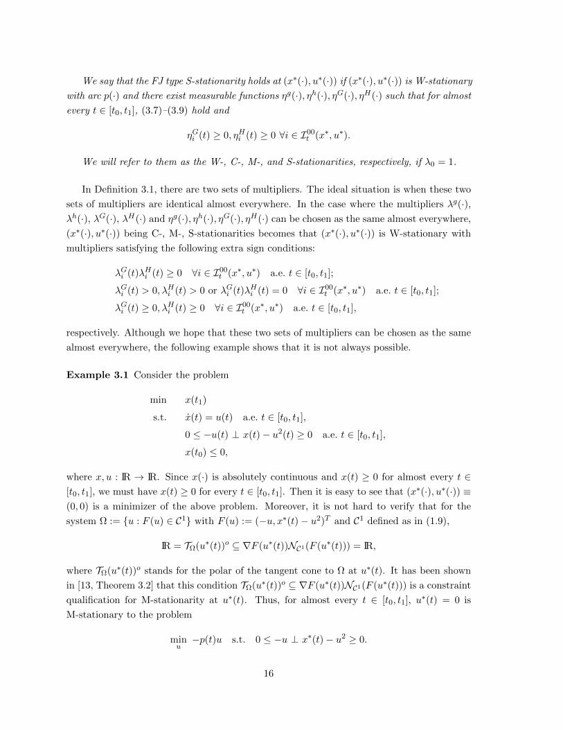
We say that the FJ type S-stationarity holds at (x∗(·), u∗(·)) if (x∗(·), u∗(·)) is W-stationary
with arc p(·) and there exist measurable functions ηg(·), ηh(·), ηG(·), ηH(·) such that for almost
every t ∈ [t0, t1], (3.7)–(3.9) hold and
ηGi (t) ≥ 0, ηHi (t) ≥ 0 ∀i ∈ I00t (x∗, u∗).
We will refer to them as the W-, C-, M-, and S-stationarities, respectively, if λ0 = 1.
In Definition 3.1, there are two sets of multipliers. The ideal situation is when these two
sets of multipliers are identical almost everywhere. In the case where the multipliers λg(·),λh(·), λG(·), λH(·) and ηg(·), ηh(·), ηG(·), ηH(·) can be chosen as the same almost everywhere,
(x∗(·), u∗(·)) being C-, M-, S-stationarities becomes that (x∗(·), u∗(·)) is W-stationary with
multipliers satisfying the following extra sign conditions:
λGi (t)λHi (t) ≥ 0 ∀i ∈ I00t (x∗, u∗) a.e. t ∈ [t0, t1];
λGi (t) > 0, λHi (t) > 0 or λGi (t)λHi (t) = 0 ∀i ∈ I00t (x∗, u∗) a.e. t ∈ [t0, t1];
λGi (t) ≥ 0, λHi (t) ≥ 0 ∀i ∈ I00t (x∗, u∗) a.e. t ∈ [t0, t1],
respectively. Although we hope that these two sets of multipliers can be chosen as the same
almost everywhere, the following example shows that it is not always possible.
Example 3.1 Consider the problem
min x(t1)
s.t. x(t) = u(t) a.e. t ∈ [t0, t1],
0 ≤ −u(t) ⊥ x(t)− u2(t) ≥ 0 a.e. t ∈ [t0, t1],
x(t0) ≤ 0,
where x, u : IR → IR. Since x(·) is absolutely continuous and x(t) ≥ 0 for almost every t ∈[t0, t1], we must have x(t) ≥ 0 for every t ∈ [t0, t1]. Then it is easy to see that (x∗(·), u∗(·)) ≡(0, 0) is a minimizer of the above problem. Moreover, it is not hard to verify that for the
system Ω := u : F (u) ∈ C1 with F (u) := (−u, x∗(t)− u2)T and C1 defined as in (1.9),
IR = TΩ(u∗(t))o ⊆ ∇F (u∗(t))NC1(F (u∗(t))) = IR,
where TΩ(u∗(t))o stands for the polar of the tangent cone to Ω at u∗(t). It has been shown
in [13, Theorem 3.2] that this condition TΩ(u∗(t))o ⊆ ∇F (u∗(t))NC1(F (u∗(t))) is a constraint
qualification for M-stationarity at u∗(t). Thus, for almost every t ∈ [t0, t1], u∗(t) = 0 is
M-stationary to the problem
minu−p(t)u s.t. 0 ≤ −u ⊥ x∗(t)− u2 ≥ 0.
16
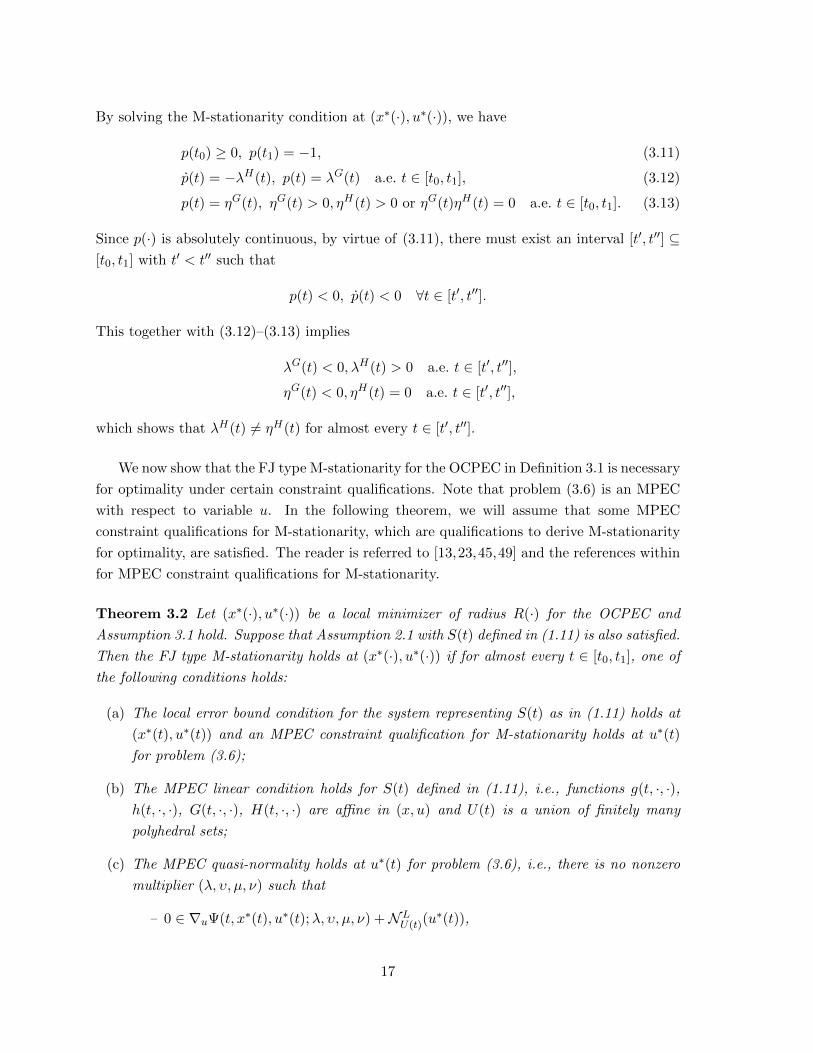
By solving the M-stationarity condition at (x∗(·), u∗(·)), we have
p(t0) ≥ 0, p(t1) = −1, (3.11)
p(t) = −λH(t), p(t) = λG(t) a.e. t ∈ [t0, t1], (3.12)
p(t) = ηG(t), ηG(t) > 0, ηH(t) > 0 or ηG(t)ηH(t) = 0 a.e. t ∈ [t0, t1]. (3.13)
Since p(·) is absolutely continuous, by virtue of (3.11), there must exist an interval [t′, t′′] ⊆[t0, t1] with t′ < t′′ such that
p(t) < 0, p(t) < 0 ∀t ∈ [t′, t′′].
This together with (3.12)–(3.13) implies
λG(t) < 0, λH(t) > 0 a.e. t ∈ [t′, t′′],
ηG(t) < 0, ηH(t) = 0 a.e. t ∈ [t′, t′′],
which shows that λH(t) 6= ηH(t) for almost every t ∈ [t′, t′′].
We now show that the FJ type M-stationarity for the OCPEC in Definition 3.1 is necessary
for optimality under certain constraint qualifications. Note that problem (3.6) is an MPEC
with respect to variable u. In the following theorem, we will assume that some MPEC
constraint qualifications for M-stationarity, which are qualifications to derive M-stationarity
for optimality, are satisfied. The reader is referred to [13,23,45,49] and the references within
for MPEC constraint qualifications for M-stationarity.
Theorem 3.2 Let (x∗(·), u∗(·)) be a local minimizer of radius R(·) for the OCPEC and
Assumption 3.1 hold. Suppose that Assumption 2.1 with S(t) defined in (1.11) is also satisfied.
Then the FJ type M-stationarity holds at (x∗(·), u∗(·)) if for almost every t ∈ [t0, t1], one of
the following conditions holds:
(a) The local error bound condition for the system representing S(t) as in (1.11) holds at
(x∗(t), u∗(t)) and an MPEC constraint qualification for M-stationarity holds at u∗(t)
for problem (3.6);
(b) The MPEC linear condition holds for S(t) defined in (1.11), i.e., functions g(t, ·, ·),h(t, ·, ·), G(t, ·, ·), H(t, ·, ·) are affine in (x, u) and U(t) is a union of finitely many
polyhedral sets;
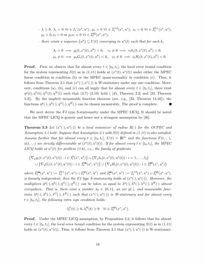
(c) The MPEC quasi-normality holds at u∗(t) for problem (3.6), i.e., there is no nonzero
multiplier (λ, υ, µ, ν) such that
– 0 ∈ ∇uΨ(t, x∗(t), u∗(t);λ, υ, µ, ν) +NLU(t)(u
∗(t)),
17
– λ ≥ 0, λi = 0 ∀i ∈ I−t (x∗, u∗), µi = 0 ∀i ∈ I+0t (x∗, u∗), νi = 0 ∀i ∈ I0+
t (x∗, u∗),
µi > 0, νi > 0 or µiνi = 0 ∀i ∈ I00t (x∗, u∗),
– there exists a sequence uk ⊆ U(t) converging to u∗(t) such that for each k,
λi > 0 =⇒ gi(t, x∗(t), uk) > 0, υi 6= 0 =⇒ υihi(t, x
∗(t), uk) > 0,
µi 6= 0 =⇒ µiGi(t, x∗(t), uk) < 0, νi 6= 0 =⇒ νiHi(t, x
∗(t), uk) < 0.
Proof. First we observe that for almost every t ∈ [t0, t1], the local error bound condition
for the system representing S(t) as in (1.11) holds at (x∗(t), u∗(t)) under either the MPEC
linear condition in condition (b) or the MPEC quasi-normality in condition (c). Thus, it
follows from Theorem 3.1 that (x∗(·), u∗(·)) is W-stationary under any one condition. More-
over, conditions (a), (b), and (c) can all imply that for almost every t ∈ [t0, t1], there exist
ηg(t), ηh(t), ηG(t), ηH(t) such that (3.7)–(3.10) hold ( [45, Theorem 2.2] and [23, Theorem
3.3]). By the implicit measurable function theorem (see, e.g., [33, Theorem 14.16]), the
functions ηg(·), ηh(·), ηG(·), ηH(·) can be chosen measurably. The proof is complete.
We next derive the FJ type S-stationarity under the MPEC LICQ. It should be noted
that the MPEC LICQ is generic and hence not a stringent assumption by [36].
Theorem 3.3 Let (x∗(·), u∗(·)) be a local minimizer of radius R(·) for the OCPEC and
Assumption 3.1 hold. Suppose that Assumption 2.1 with S(t) defined in (1.11) is also satisfied.
Assume further that for almost every t ∈ [t0, t1], U(t) = IRm and the functions F (t, ·, ·),φ(t, ·, ·) are strictly differentiable at (x∗(t), u∗(t)). If for almost every t ∈ [t0, t1], the MPEC
LICQ holds at u∗(t) for problem (3.6), i.e., the family of gradients∇ugi(t, x∗(t), u∗(t)) : i ∈ I0
t (x∗, u∗)∪ ∇uhi(t, x∗(t), u∗(t)) : i = 1, . . . , l2
∪∇uGi(t, x∗(t), u∗(t)) : i ∈ I0•
t (x∗, u∗)∪∇uHi(t, x
∗(t), u∗(t)) : i ∈ I•0t (x∗, u∗)
where I0•t (x∗, u∗) := I0+
t (x∗, u∗) ∪ I00t (x∗, u∗) and I•0t (x∗, u∗) := I+0
t (x∗, u∗) ∪ I00t (x∗, u∗),
is linearly independent, then the FJ type S-stationarity holds at (x∗(·), u∗(·)). Moreover, the
multipliers ηg(·), ηh(·), ηG(·), ηH(·) can be taken as equal to λg(·), λh(·), λG(·), λH(·) almost
everywhere. That is, there exist a number λ0 ∈ 0, 1, an arc p(·), and measurable func-
tions λg(·), λh(·), λG(·), λH(·) such that (x∗(·), u∗(·)) is W-stationary and for almost every
t ∈ [t0, t1], the following extra sign condition holds:
λGi (t) ≥ 0, λHi (t) ≥ 0 ∀i ∈ I00t (x∗, u∗).
Proof. Under the MPEC LICQ assumption, by Proposition 2.2, it follows that for almost
every t ∈ [t0, t1], the local error bound condition for the system representing S(t) as in (1.11)
holds at (x∗(t), u∗(t)). Thus, it follows from Theorem 3.1 that (x∗(·), u∗(·)) is W-stationary.
18
Moreover, for almost every t ∈ [t0, t1], since the MPEC LICQ holds at u∗(t), it then follows
from [35, Theorem 2] that there exist ηg(t), ηh(t), ηG(t), ηH(t) such that (3.7)–(3.9) hold and
ηGi (t) ≥ 0, ηHi (t) ≥ 0 i ∈ I00t (x∗, u∗).
By the implicit measurable function theorem (see, e.g., [33, Theorem 14.16]), the functions
ηg(·), ηh(·), ηG(·), ηH(·) can be chosen measurably. Thus, the first part of the theorem is
derived. Moreover, by the MPEC-LICQ assumption, it is not hard to see that λg(t) =
ηg(t), λg(t) = ηg(t), λG(t) = ηG(t), λH(t) = ηH(t) for almost every t ∈ [t0, t1]. Therefore, the
second part of the theorem follows immediately. The proof is complete.
For problem (Ps), if S(t) = IRn × U(t) for almost every t ∈ [t0, t1] (which corresponds to
the case of standard optimal control problem without mixed constraints), then the bounded
slope condition (2.4) holds automatically for almost every t ∈ [t0, t1] since in this case, (2.4)
becomes
(x, u) ∈ Sε,R∗ (t), β ∈ NPU(t)(u) =⇒ kS(t)‖β‖ ≥ 0,
which holds trivially if kS(t) ≥ 0. If there exists a closed subset X(t′) ⊆ IRn and x∗(t′) ∈bdX(t′) satisfying S(t′) = X(t′)× IRm and
distbdX(t′)(x∗(t′)) = ‖x∗(t′)− x∗(t′)‖ ≤ ε,
then (2.4) at time t′ never hold since there exists 0 6= α ∈ NPX(t′)(x
∗(t′)) by [33, Exercise 6.19].
If the set of such a point t′ ∈ [t0, t1] is not of measure zero, then the bounded slope condition
in Assumption 2.1 does not hold. As a consequence, the bounded slope condition can hardly
hold for the case of the pure state constraint S(t) = X(t) × IRm. Generally speaking, the
bounded slope condition is a strong condition and is also hard to verify. In the rest of this
section, we will investigate sufficient conditions for the bounded slope condition to hold in
our problem setting.
Proposition 3.1 Assume that the local error bound condition for the system representing
S(t) as in (1.11) holds at every (x, u) ∈ Sε,R∗ (t) and(x, u) ∈ Sε,R∗ (t), ζ ∈ NL
U(t)(u),
λ ≥ 0, λi = 0 ∀i ∈ I−t (x, u),
µi = 0 ∀i ∈ I+0t (x, u), νi = 0 ∀i ∈ I0+
t (x, u),
µi > 0, νi > 0 or µiνi = 0 ∀i ∈ I00t (x, u),
=⇒ ‖∇xΨ(t, x, u;λ, υ, µ, ν)‖ ≤ kS(t)‖∇uΨ(t, x, u;λ, υ, µ, ν) + ζ‖. (3.14)
Then the bounded slope condition (2.4) holds.
Proof. Let (x, u) ∈ Sε,R∗ (t) and (α, β) ∈ NLS(t)(x, u). Since the local error bound condition
holds at (x, u), it then follows from [22, Proposition 3.4] that
(α, β) ∈
∇x,uΨ(t, x, u;λ, υ, µ, ν) :
λ ∈ NL
IRl1−
(g(t, x, u)), υ ∈ IRl2
(µ, ν) ∈ NLCl(G(t, x, u), H(t, x, u))
+ 0 × NL
U(t)(u).
19
Then, by Proposition 2.1, there exist λ, υ, µ, ν such that
(α, β) ∈ ∇x,uΨ(t, x, u;λ, υ, µ, ν) + 0 × NLU(t)(u), λ ≥ 0, λi = 0 ∀i ∈ I−t (x, u),
µi = 0 ∀i ∈ I+0t (x, u), νi = 0 ∀i ∈ I0+
t (x, u), µi > 0, νi > 0 or µiνi = 0 ∀i ∈ I00t (x, u).
It then follows that there exists ζ ∈ NLU(t)(u) such that
α = ∇xΨ(t, x, u;λ, υ, µ, ν), β = ∇uΨ(t, x, u;λ, υ, µ, ν) + ζ.
Thus, by condition (3.14), we have ‖α‖ ≤ kS(t)‖β‖. The proof is complete.
A sufficient condition for condition (3.14) to hold is the following stronger condition that
is similar to the M ε,R∗ condition given in [7]: There exists a measurable function κ(·) such
that for almost every t ∈ [t0, t1],(x, u) ∈ Sε,R∗ (t), ζ ∈ NL
U(t)(u),
λ ≥ 0, λi = 0 ∀i ∈ I−t (x, u),
µi = 0 ∀i ∈ I+0t (x, u), νi = 0 ∀i ∈ I0+
t (x, u),
µi > 0, νi > 0 or µiνi = 0 ∀i ∈ I00t (x, u),
=⇒ ‖(λ, υ, µ, ν)‖ ≤ κ(t)‖∇uΨ(t, x, u;λ, υ, µ, ν) + ζ‖. (3.15)
Assumption 3.2 There exist measurable functions kgx(·), khx(·), kGx (·), kHx (·) such that for al-
most every t ∈ [t0, t1],
‖g(t, x1, u)− g(t, x2, u)‖ ≤ kgx(t)‖x1 − x2‖ ∀(x1, u), (x2, u) ∈ Sε,R∗ (t),
‖h(t, x1, u)− h(t, x2, u)‖ ≤ khx(t)‖x1 − x2‖ ∀(x1, u), (x2, u) ∈ Sε,R∗ (t),
‖G(t, x1, u)−G(t, x2, u)‖ ≤ kGx (t)‖x1 − x2‖ ∀(x1, u), (x2, u) ∈ Sε,R∗ (t),
‖H(t, x1, u)−H(t, x2, u)‖ ≤ kHx (t)‖x1 − x2‖ ∀(x1, u), (x2, u) ∈ Sε,R∗ (t).
Proposition 3.2 Let Assumption 3.2 and condition (3.15) hold. Then the local error bound
condition for the system representing S(t) as in (1.11) holds at every (x, u) ∈ Sε,R∗ (t) and the
bounded slope condition (2.4) holds with kS(t) = κ(t)(kgx(t) + khx(t) + kGx (t) + kHx (t)).
Proof. Let (x, u) ∈ Sε,R∗ (t). It is not hard to verify that condition (3.15) implies that0 ∈ ∇uΨ(t, x, u;λ, υ, µ, ν) +NL
U(t)(u),
λ ≥ 0, λi = 0 ∀i ∈ I−t (x, u),
µi = 0 ∀i ∈ I+0t (x, u), νi = 0 ∀i ∈ I0+
t (x, u),
µi > 0, νi > 0 or µiνi = 0 ∀i ∈ I00t (x, u),
=⇒ (λ, υ, µ, ν) = 0.
This indicates that the MPEC quasi-normality holds at (x, u) and then by Proposition 2.2,
the local error bound condition for the system representing S(t) as in (1.11) holds at (x, u).
20
In the same way as in [7, Proposition 4.2], we can have that condition (3.14) holds with
kS(t) := κ(t)(kgx(t) + khx(t) + kGx (t) + kHx (t)). Consequently, the bounded slope condition
follows from Proposition 3.1 immediately. The proof is complete.
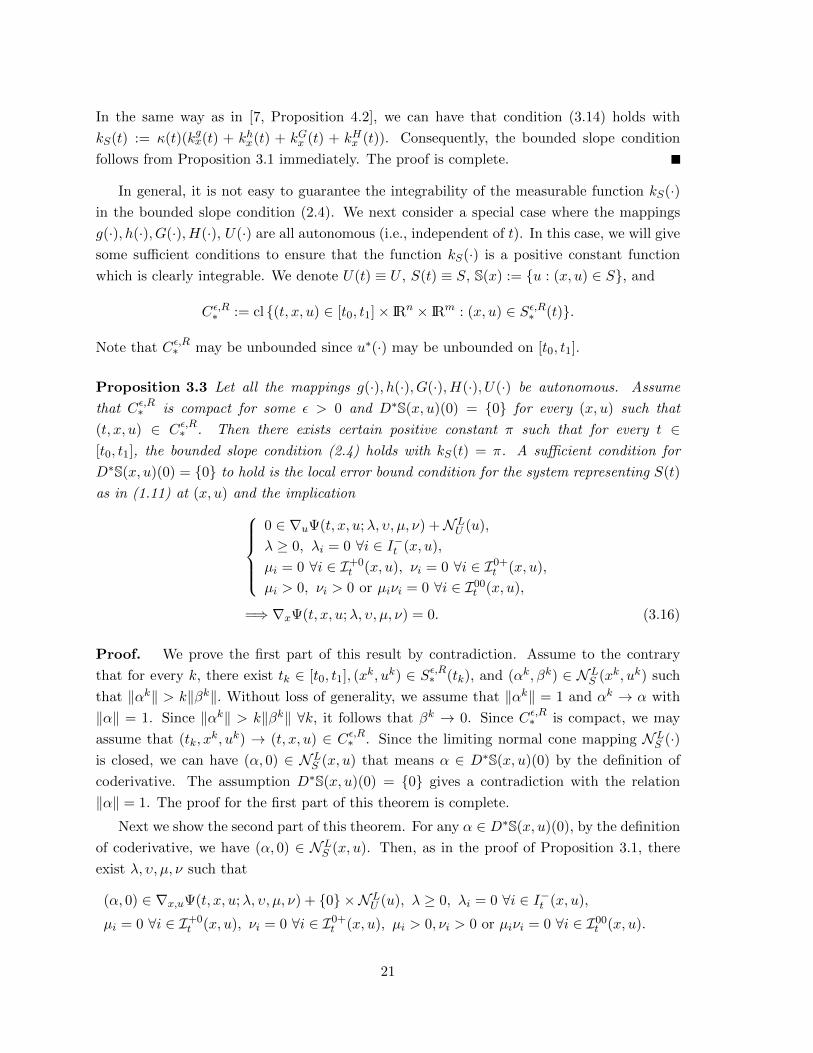
In general, it is not easy to guarantee the integrability of the measurable function kS(·)in the bounded slope condition (2.4). We next consider a special case where the mappings
g(·), h(·), G(·), H(·), U(·) are all autonomous (i.e., independent of t). In this case, we will give
some sufficient conditions to ensure that the function kS(·) is a positive constant function
which is clearly integrable. We denote U(t) ≡ U , S(t) ≡ S, S(x) := u : (x, u) ∈ S, and
Cε,R∗ := cl (t, x, u) ∈ [t0, t1]× IRn × IRm : (x, u) ∈ Sε,R∗ (t).
Note that Cε,R∗ may be unbounded since u∗(·) may be unbounded on [t0, t1].
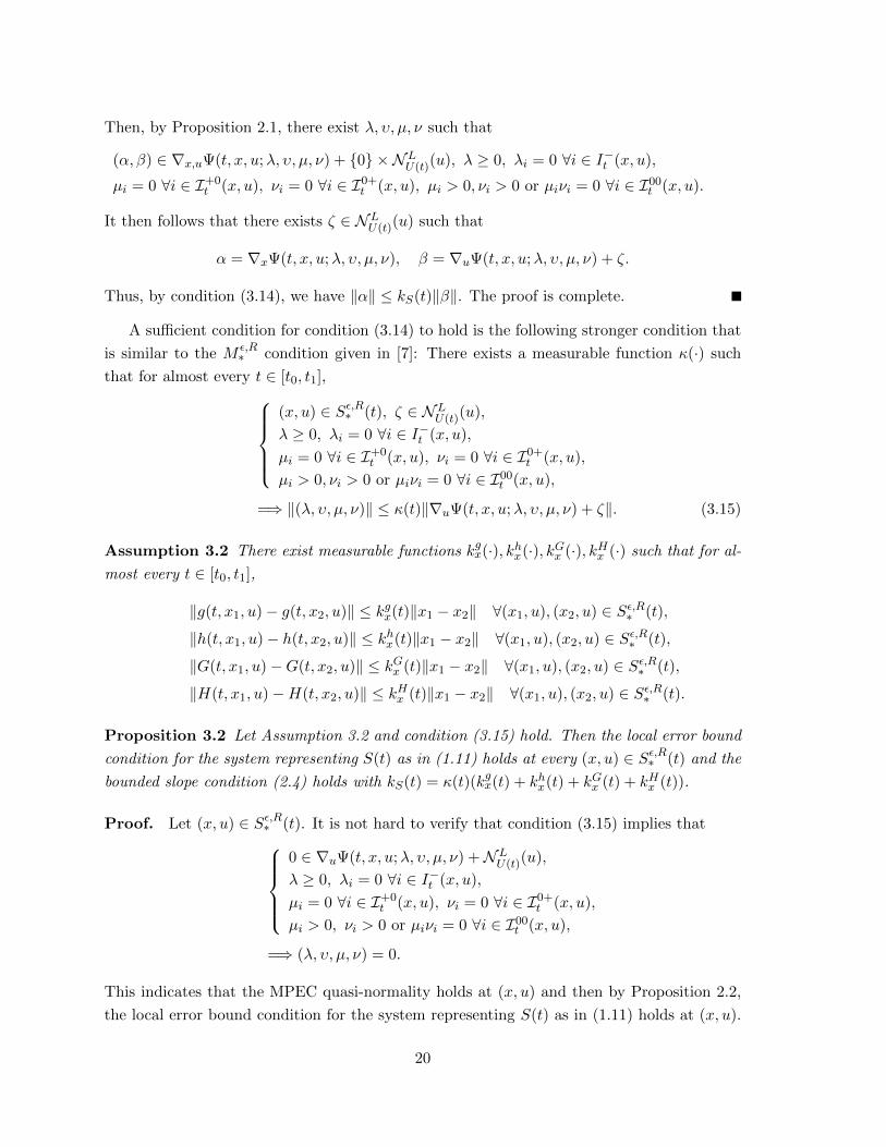
Proposition 3.3 Let all the mappings g(·), h(·), G(·), H(·), U(·) be autonomous. Assume
that Cε,R∗ is compact for some ε > 0 and D∗S(x, u)(0) = 0 for every (x, u) such that
(t, x, u) ∈ Cε,R∗ . Then there exists certain positive constant π such that for every t ∈[t0, t1], the bounded slope condition (2.4) holds with kS(t) = π. A sufficient condition for
D∗S(x, u)(0) = 0 to hold is the local error bound condition for the system representing S(t)
as in (1.11) at (x, u) and the implication0 ∈ ∇uΨ(t, x, u;λ, υ, µ, ν) +NL
U (u),
λ ≥ 0, λi = 0 ∀i ∈ I−t (x, u),
µi = 0 ∀i ∈ I+0t (x, u), νi = 0 ∀i ∈ I0+
t (x, u),
µi > 0, νi > 0 or µiνi = 0 ∀i ∈ I00t (x, u),
=⇒ ∇xΨ(t, x, u;λ, υ, µ, ν) = 0. (3.16)
Proof. We prove the first part of this result by contradiction. Assume to the contrary
that for every k, there exist tk ∈ [t0, t1], (xk, uk) ∈ Sε,R∗ (tk), and (αk, βk) ∈ NLS (xk, uk) such
that ‖αk‖ > k‖βk‖. Without loss of generality, we assume that ‖αk‖ = 1 and αk → α with
‖α‖ = 1. Since ‖αk‖ > k‖βk‖ ∀k, it follows that βk → 0. Since Cε,R∗ is compact, we may
assume that (tk, xk, uk) → (t, x, u) ∈ Cε,R∗ . Since the limiting normal cone mapping NL
S (·)is closed, we can have (α, 0) ∈ NL
S (x, u) that means α ∈ D∗S(x, u)(0) by the definition of
coderivative. The assumption D∗S(x, u)(0) = 0 gives a contradiction with the relation
‖α‖ = 1. The proof for the first part of this theorem is complete.
Next we show the second part of this theorem. For any α ∈ D∗S(x, u)(0), by the definition
of coderivative, we have (α, 0) ∈ NLS (x, u). Then, as in the proof of Proposition 3.1, there
exist λ, υ, µ, ν such that
(α, 0) ∈ ∇x,uΨ(t, x, u;λ, υ, µ, ν) + 0 × NLU (u), λ ≥ 0, λi = 0 ∀i ∈ I−t (x, u),
µi = 0 ∀i ∈ I+0t (x, u), νi = 0 ∀i ∈ I0+
t (x, u), µi > 0, νi > 0 or µiνi = 0 ∀i ∈ I00t (x, u).
21
It then follows that
α = ∇xΨ(t, x, u;λ, υ, µ, ν), 0 ∈ ∇uΨ(t, x, u;λ, υ, µ, ν) +NLU (u),
which together with condition (3.16) implies that α = 0. The proof for the second part of
the theorem is complete.
The following condition that is stronger than condition (3.16) is similar to the so-called
MFC proposed in [7]: 0 ∈ ∇uΨ(t, x, u;λ, υ, µ, ν) +NL
U (u),
λ ≥ 0, λi = 0 ∀i ∈ I−t (x, u),
µi = 0 ∀i ∈ I+0t (x, u), νi = 0 ∀i ∈ I0+
t (x, u),
µi > 0, νi > 0 or µiνi = 0 ∀i ∈ I00t (x, u),
=⇒ (λ, υ, µ, ν) = 0, (3.17)
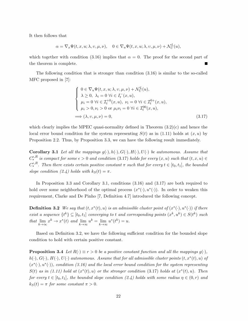
which clearly implies the MPEC quasi-normality defined in Theorem (3.2)(c) and hence the
local error bound condition for the system representing S(t) as in (1.11) holds at (x, u) by
Proposition 2.2. Thus, by Proposition 3.3, we can have the following result immediately.
Corollary 3.1 Let all the mappings g(·), h(·), G(·), H(·), U(·) be autonomous. Assume that
Cε,R∗ is compact for some ε > 0 and condition (3.17) holds for every (x, u) such that (t, x, u) ∈Cε,R∗ . Then there exists certain positive constant π such that for every t ∈ [t0, t1], the bounded
slope condition (2.4) holds with kS(t) = π.
In Proposition 3.3 and Corollary 3.1, conditions (3.16) and (3.17) are both required to
hold over some neighborhood of the optimal process (x∗(·), u∗(·)). In order to weaken this
requirement, Clarke and De Pinho [7, Definition 4.7] introduced the following concept.
Definition 3.2 We say that (t, x∗(t), u) is an admissible cluster point of (x∗(·), u∗(·)) if there
exist a sequence tk ⊆ [t0, t1] converging to t and corresponding points (xk, uk) ∈ S(tk) such
that limk→∞
xk → x∗(t) and limk→∞
uk = limk→∞
u∗(tk) = u.
Based on Definition 3.2, we have the following sufficient condition for the bounded slope
condition to hold with certain positive constant.
Proposition 3.4 Let R(·) ≡ r > 0 be a positive constant function and all the mappings g(·),h(·), G(·), H(·), U(·) autonomous. Assume that for all admissible cluster points (t, x∗(t), u) of
(x∗(·), u∗(·)), condition (3.16) and the local error bound condition for the system representing
S(t) as in (1.11) hold at (x∗(t), u) or the stronger condition (3.17) holds at (x∗(t), u). Then
for every t ∈ [t0, t1], the bounded slope condition (2.4) holds with some radius η ∈ (0, r) and
kS(t) = π for some constant π > 0.
22
Proof. Mimicking the proof of Proposition 3.3, we can show that there exist ε1 ∈ (0, ε),
η ∈ (0, r), and π > 0 such that for every t ∈ [t0, t1], the following bounded slope condition
holds:
(x, u) ∈ Sε1,η∗ (t), (α, β) ∈ NPS (x, u) =⇒ ‖α‖ ≤ π‖β‖.
The proof is complete.
Although all the mappings g(·), h(·), G(·), H(·), U(·) are assumed to be autonomous in
Propositions 3.3–3.4 and Corollary 3.1, their results can be applied to the non-autonomous
case if U(t) ≡ U is autonomous and we treat the time variable t as a state variable. We now
illustrate how this can be done. Since
σ(t) = t ∀t ∈ [t0, t1]⇐⇒ σ(t) = 1 ∀t ∈ [t0, t1], σ(t0) = t0, (3.18)
it is clear that the OCPEC is equivalent to the following optimal control problem:
min J(x(·), u(·)) :=
∫ t1
t0
F (σ(t), x(t), u(t))dt+ f(x(t0), x(t1)),
s.t. x(t) = φ(σ(t), x(t), u(t)), σ(t) = 1 a.e. t ∈ [t0, t1],
g(σ(t), x(t), u(t)) ≤ 0, h(σ(t), x(t), u(t)) = 0 a.e. t ∈ [t0, t1],
0 ≤ G(σ(t), x(t), u(t)) ⊥ H(σ(t), x(t), u(t)) ≥ 0 a.e. t ∈ [t0, t1],
u(t) ∈ U a.e. t ∈ [t0, t1],
σ(t0) = t0, (x(t0), x(t1)) ∈ E.
It is easy to see that (σ(·), x∗(·), u∗(·)) is a local minimizer of radius R(·) for the above
problem if (x∗(·), u∗(·)) is a local minimizer of radius R(·) for the OCPEC and σ(·) is defined
in (3.18). Thus, the results in Propositions 3.3–3.4 and Corollary 3.1 can be applied to the
above problem to get the desired result.
We close this section by noting the equivalence of the S-stationarity for the OCPEC and
the classical necessary optimality condition for the OCPEC treated as an optimal control
problem with mixed inequality constraints (1.8). The proof for the following result is similar
to [12, Proposition 4.1] and we omit the proof here.
Proposition 3.5 (x∗(·), u∗(·)) is an FJ type stationary solution of the OCPEC treated as an
optimal control problem with mixed inequality constraints (1.8) if and only if (x∗(·), u∗(·)) is
an FJ type S-stationary solution of the OCPEC for which those two sets of multipliers can
be chosen as the same.
4 A simple example
In this section, we consider a simple class of the OCPEC in which the “best” control needs to
be chosen from the DCP (1.3) so as to make the final state x(t1) reach some prescribed target
23
T from a given initial state x(t0). Mathematically, the problem considered in this section is
min 12‖x(t1)− T ‖2
x(t) = φ(t, x(t), u(t)) a.e. t ∈ [t0, t1],
0 ≤ u(t) ⊥ Υ(t, x(t), u(t)) ≥ 0 a.e. t ∈ [t0, t1],
x(t0) ∈ E0,
(4.1)
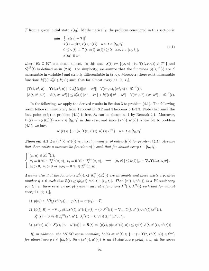
where E0 ⊆ IRn is a closed subset. In this case, S(t) := (x, u) : (u,Υ(t, x, u)) ∈ Cm and
Sε,R∗ (t) is defined as in (2.3). For simplicity, we assume that the functions φ(·),Υ(·) are Lmeasurable in variable t and strictly differentiable in (x, u). Moreover, there exist measurable
functions kφx(·), kφu(·), kΥx (·) such that for almost every t ∈ [t0, t1],
‖Υ(t, x1, u)−Υ(t, x2, u)‖ ≤ kΥx (t)‖x1 − x2‖ ∀(x1, u), (x2, u) ∈ Sε,R∗ (t),
‖φ(t, x1, u1)− φ(t, x2, u2)‖ ≤ kφx(t)‖x1 − x2‖+ kφu(t)‖u1 − u2‖ ∀(x1, u1), (x2, u2) ∈ Sε,R∗ (t).
In the following, we apply the derived results in Section 3 to problem (4.1). The following
result follows immediately from Proposition 3.2 and Theorems 3.1–3.3. Note that since the
final point x(t1) in problem (4.1) is free, λ0 can be chosen as 1 by Remark 2.1. Moreover,
kS(t) = κ(t)kΥx (t) a.e. t ∈ [t0, t1] in this case, and since (x∗(·), u∗(·)) is feasible to problem
(4.1), we have
u∗(t) ∈ u : (u,Υ(t, x∗(t), u)) ∈ Cm a.e. t ∈ [t0, t1].
Theorem 4.1 Let (x∗(·), u∗(·)) be a local minimizer of radius R(·) for problem (4.1). Assume
that there exists a measurable function κ(·) such that for almost every t ∈ [t0, t1],(x, u) ∈ Sε,R∗ (t),
µi = 0 ∀i ∈ I+0t (x, u), νi = 0 ∀i ∈ I0+
t (x, u),
µi > 0, νi > 0 or µiνi = 0 ∀i ∈ I00t (x, u),
=⇒ ‖(µ, ν)‖ ≤ κ(t)‖µ+∇uΥ(t, x, u)ν‖.
Assume also that the functions kφx(·), κ(·)kΥx (·)kφu(·) are integrable and there exists a positive
number η > 0 such that R(t) ≥ ηkS(t) a.e. t ∈ [t0, t1]. Then (x∗(·), u∗(·)) is a W-stationary
point, i.e., there exist an arc p(·) and measurable functions λG(·), λH(·) such that for almost
every t ∈ [t0, t1],
1) p(t0) ∈ NLE0
(x∗(t0)), −p(t1) = x∗(t1)− T ,
2) (p(t), 0) = −∇x,uφ(t, x∗(t), u∗(t))p(t)− (0, λG(t))−∇x,uΥ(t, x∗(t), u∗(t))λH(t),
λGi (t) = 0 ∀i ∈ I+0t (x∗, u∗), λHi (t) = 0 ∀i ∈ I0+
t (x∗, u∗),
3) (x∗(t), u) ∈ S(t), ‖u− u∗(t))‖ < R(t)⇒ 〈p(t), φ(t, x∗(t), u)〉 ≤ 〈p(t), φ(t, x∗(t), u∗(t))〉.
If, in addition, the MPEC quasi-normality holds at u∗(t) ∈ u : (u,Υ(t, x∗(t), u)) ∈ Cmfor almost every t ∈ [t0, t1], then (x∗(·), u∗(·)) is an M-stationary point, i.e., all the above
24
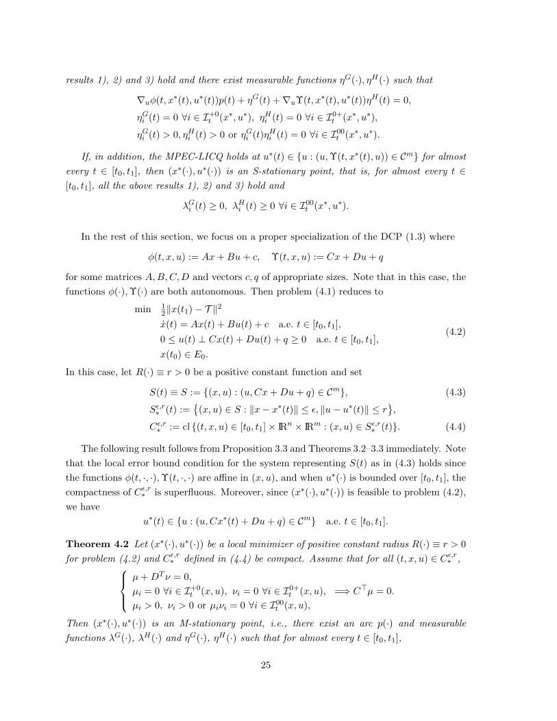
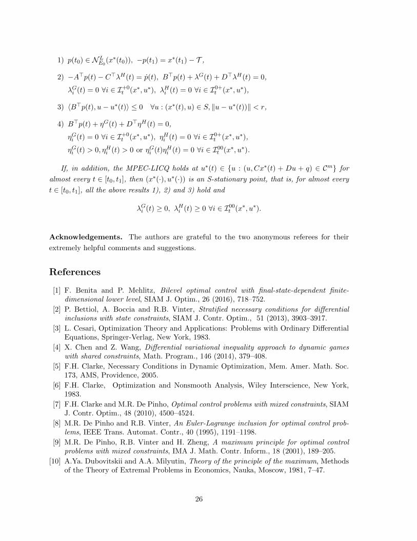
results 1), 2) and 3) hold and there exist measurable functions ηG(·), ηH(·) such that
∇uφ(t, x∗(t), u∗(t))p(t) + ηG(t) +∇uΥ(t, x∗(t), u∗(t))ηH(t) = 0,
ηGi (t) = 0 ∀i ∈ I+0t (x∗, u∗), ηHi (t) = 0 ∀i ∈ I0+
t (x∗, u∗),
ηGi (t) > 0, ηHi (t) > 0 or ηGi (t)ηHi (t) = 0 ∀i ∈ I00t (x∗, u∗).
If, in addition, the MPEC-LICQ holds at u∗(t) ∈ u : (u,Υ(t, x∗(t), u)) ∈ Cm for almost
every t ∈ [t0, t1], then (x∗(·), u∗(·)) is an S-stationary point, that is, for almost every t ∈[t0, t1], all the above results 1), 2) and 3) hold and
λGi (t) ≥ 0, λHi (t) ≥ 0 ∀i ∈ I00t (x∗, u∗).
In the rest of this section, we focus on a proper specialization of the DCP (1.3) where
φ(t, x, u) := Ax+Bu+ c, Υ(t, x, u) := Cx+Du+ q
for some matrices A,B,C,D and vectors c, q of appropriate sizes. Note that in this case, the
functions φ(·),Υ(·) are both autonomous. Then problem (4.1) reduces to
min 12‖x(t1)− T ‖2
x(t) = Ax(t) +Bu(t) + c a.e. t ∈ [t0, t1],
0 ≤ u(t) ⊥ Cx(t) +Du(t) + q ≥ 0 a.e. t ∈ [t0, t1],
x(t0) ∈ E0.
(4.2)
In this case, let R(·) ≡ r > 0 be a positive constant function and set
S(t) ≡ S := (x, u) : (u,Cx+Du+ q) ∈ Cm, (4.3)
Sε,r∗ (t) :=
(x, u) ∈ S : ‖x− x∗(t)‖ ≤ ε, ‖u− u∗(t)‖ ≤ r,
Cε,r∗ := cl (t, x, u) ∈ [t0, t1]× IRn × IRm : (x, u) ∈ Sε,r∗ (t). (4.4)
The following result follows from Proposition 3.3 and Theorems 3.2–3.3 immediately. Note
that the local error bound condition for the system representing S(t) as in (4.3) holds since
the functions φ(t, ·, ·),Υ(t, ·, ·) are affine in (x, u), and when u∗(·) is bounded over [t0, t1], the
compactness of Cε,r∗ is superfluous. Moreover, since (x∗(·), u∗(·)) is feasible to problem (4.2),
we have
u∗(t) ∈ u : (u,Cx∗(t) +Du+ q) ∈ Cm a.e. t ∈ [t0, t1].
Theorem 4.2 Let (x∗(·), u∗(·)) be a local minimizer of positive constant radius R(·) ≡ r > 0
for problem (4.2) and Cε,r∗ defined in (4.4) be compact. Assume that for all (t, x, u) ∈ Cε,r∗ ,µ+DT ν = 0,
µi = 0 ∀i ∈ I+0t (x, u), νi = 0 ∀i ∈ I0+
t (x, u),
µi > 0, νi > 0 or µiνi = 0 ∀i ∈ I00t (x, u),
=⇒ C>µ = 0.
Then (x∗(·), u∗(·)) is an M-stationary point, i.e., there exist an arc p(·) and measurable
functions λG(·), λH(·) and ηG(·), ηH(·) such that for almost every t ∈ [t0, t1],
25
1) p(t0) ∈ NLE0
(x∗(t0)), −p(t1) = x∗(t1)− T ,
2) −A>p(t)− C>λH(t) = p(t), B>p(t) + λG(t) +D>λH(t) = 0,
λGi (t) = 0 ∀i ∈ I+0t (x∗, u∗), λHi (t) = 0 ∀i ∈ I0+
t (x∗, u∗),
3) 〈B>p(t), u− u∗(t)〉 ≤ 0 ∀u : (x∗(t), u) ∈ S, ‖u− u∗(t))‖ < r,
4) B>p(t) + ηG(t) +D>ηH(t) = 0,
ηGi (t) = 0 ∀i ∈ I+0t (x∗, u∗), ηHi (t) = 0 ∀i ∈ I0+
t (x∗, u∗),
ηGi (t) > 0, ηHi (t) > 0 or ηGi (t)ηHi (t) = 0 ∀i ∈ I00t (x∗, u∗).
If, in addition, the MPEC-LICQ holds at u∗(t) ∈ u : (u,Cx∗(t) + Du + q) ∈ Cm for
almost every t ∈ [t0, t1], then (x∗(·), u∗(·)) is an S-stationary point, that is, for almost every
t ∈ [t0, t1], all the above results 1), 2) and 3) hold and
λGi (t) ≥ 0, λHi (t) ≥ 0 ∀i ∈ I00t (x∗, u∗).
Acknowledgements. The authors are grateful to the two anonymous referees for their
extremely helpful comments and suggestions.
References
[1] F. Benita and P. Mehlitz, Bilevel optimal control with final-state-dependent finite-dimensional lower level, SIAM J. Optim., 26 (2016), 718–752.
[2] P. Bettiol, A. Boccia and R.B. Vinter, Stratified necessary conditions for differentialinclusions with state constraints, SIAM J. Contr. Optim., 51 (2013), 3903–3917.
[3] L. Cesari, Optimization Theory and Applications: Problems with Ordinary DifferentialEquations, Springer-Verlag, New York, 1983.
[4] X. Chen and Z. Wang, Differential variational inequality approach to dynamic gameswith shared constraints, Math. Program., 146 (2014), 379–408.
[5] F.H. Clarke, Necessary Conditions in Dynamic Optimization, Mem. Amer. Math. Soc.173, AMS, Providence, 2005.
[6] F.H. Clarke, Optimization and Nonsmooth Analysis, Wiley Interscience, New York,1983.
[7] F.H. Clarke and M.R. De Pinho, Optimal control problems with mixed constraints, SIAMJ. Contr. Optim., 48 (2010), 4500–4524.
[8] M.R. De Pinho and R.B. Vinter, An Euler-Lagrange inclusion for optimal control prob-lems, IEEE Trans. Automat. Contr., 40 (1995), 1191–1198.
[9] M.R. De Pinho, R.B. Vinter and H. Zheng, A maximum principle for optimal controlproblems with mixed constraints, IMA J. Math. Contr. Inform., 18 (2001), 189–205.
[10] A.Ya. Dubovitskii and A.A. Milyutin, Theory of the principle of the maximum, Methodsof the Theory of Extremal Problems in Economics, Nauka, Moscow, 1981, 7–47.
26
[11] A.F. Filippov, On certain questions in the theory of optimal control, J. Soc. Ind. Appl.Math., Ser. A: Contr., 1 (1962), 76-84.
[12] R. Fletcher, S. Leyffer, D. Ralph and S. Scholtes, Local convergence of SQP methodsfor mathematical programs with equilibrium constraints, SIAM J. Optim., 17 (2006),259–286.
[13] L. Guo and G.H. Lin, Notes on some constraint qualifications for mathematical programswith equilibrium constraints, J. Optim. Theory Appl., 156 (2013), 600–616.
[14] L. Guo, J.J. Ye and J. Zhang, Mathematical programs with geometric constraints inBanach spaces: Enhanced optimality, exact penalty, and sensitivity, SIAM J. Optim., 23(2013), 2295–2319.
[15] K. Hatz, Efficient Numerical Methods for Hierarchical Dynamic Optimization with Ap-plication to Cerebral Palsy Gait Modeling, PhD thesis, University of Heidelberg, 2014.
[16] K. Hatz, J.P. Schloder and H.G. Bock, Estimating parameters in optimal control prob-lems, SIAM J. Sci. Comput., 34 (2012), A1707–A1728.
[17] X. He, A. Prasad, S.P. Sethi and G.J. Gutierrez, A survey of Stackelberg differential gamemodels in supply and marketing channels, J. Syst. Sci. Syst. Eng., 16 (2007), 385–413.
[18] W.P.H. Heemels, Linear Complementarity Systems: A Study in Hybrid Dynamics, PhDthesis, Eindhoven University of Technology, 1999.
[19] R. Henrion and J.V. Outrata, Calmness of constraint systems with applications, Math.Program., 104 (2005), 437–464.
[20] M.R. Hestenes, Calculus of Variations and Optimal Control Theory, John Wiley & Sons,New York, 1966.
[21] M.R. Hestenes, On variational theory and optimal control theory, J. Soc. Ind. Appl.Math., Ser. A: Contr., 3 (1965), 23–48.
[22] A.D. Ioffe and J.V. Outrata, On metric and calmness qualification conditions in subdif-ferential calculus, Set-Valued Anal., 16 (2008), 199–227.
[23] C. Kanzow and A. Schwartz, Mathematical programs with equilibrium constraints: En-hanced Fritz John-conditions, new constraint qualifications, and improved exact penaltyresults, SIAM J. Optim., 20 (2010), 2730–2753.
[24] A. Li and J.J. Ye, Necessary optimality conditions for optimal control problems withnonsmooth mixed state and control constraints, Set-Valued Var. Anal. (2015), DOI10.1007/s11228-015-0358-z.
[25] N.V. Long and G. Sorger, A dynamic principal-agent problem as a feedback Stackelbergdifferential game, Centr. Eur. J. Oper. Res., 18 (2010), 491–509.
[26] Z.Q. Luo, J.S. Pang and D. Ralph, Mathematical Programs with Equilibrium Con-straints, Cambridge University Press, Cambridge, United Kingdom, 1996.
[27] B.S. Mordukhovich, Variational Analysis and Generalized Differentiation I: Basic The-ory, II: Application, Grundlehren der Mathematischen Wissenschaften 330, Springer,Berlin, 2006.
[28] J.V. Outrata, M. Kocvara and J. Zowe, Nonsmooth Approach to Optimization Problemswith Equilibrium Constraints: Theory, Applications and Numerical Results, KluwerAcademic Publishers, Boston, 1998.
[29] J.S. Pang and D.E. Stewart, Differential variational inequalities, Math. Program., 113(2008), 345–424.
[30] L.S. Pontryagin, V.F. Boltyanskii, R.V. Gamkrelidze and E. F. Mischenko, The Math-ematical Theory of Optimal Processes, John Wiley & Sons, New York, 1962.
27
[31] A.U. Raghunathan, M.S. Diaz and L.T. Biegler, An MPEC formulation for dynamicoptimization of distillation operations, Comput. Chem. Eng., 28 (2004), 2037–2052.
[32] S.M. Robinson, Some continuity properties of polyhedral multifunctions, Math. Program.,14 (1981), 206–214.
[33] R.T. Rockafellar and R.J.-B. Wets, Variational Analysis, Springer, Berlin, 1998.
[34] Y. Sannikov, A continuous-time version of the principal-agent problem, Rev. Econ. Stud.,75 (2008), 957–984.
[35] H.S. Scheel and S. Scholtes, Mathematical programs with complementarity constraints:Stationarity, optimality, and sensitivity, Math. Oper. Res., 25 (2000), 1–22.
[36] S. Scholtes and M. Stohr, How stringent is the linear independence assumption for math-ematical programs with complementarity constraints?, Math. Oper. Res., 26 (2001), 851–863.
[37] D.E. Stewart, Rigid-body dynamics with friction and impact, SIAM Rev., 42 (2000),3–39.
[38] R.B. Vinter, Optimal Control, Birkhauser Boston, Boston, 2000.
[39] J. Warga, Optimal Control of Differential and Functional Equations, Academic Press,New York, 1972.
[40] Z. Wu and J.J. Ye, Sufficient conditions for error bounds, SIAM J. Optim., 12 (2002),421–435.
[41] Z. Wu and J.J. Ye, On error bounds for lower semicontinuous functions, SIAM J. Optim.,92 (2002), 301–314.
[42] Z. Wu and J.J. Ye, First-order and second-order conditions for error bounds, SIAM J.Optim., 14 (2004), 621–645.
[43] D. Xie, On time inconsistency: A technical issue in Stackelberg differential games, J.Econ. Theory, 76 (1997), 412–430.
[44] J.J. Ye, Constraint qualifications and necessary optimality conditions for optimizationproblems with variational inequality constraints, SIAM J. Optim., 10 (2000), 943–962.
[45] J.J. Ye, Necessary and sufficient optimality conditions for mathematical programs withequilibrium constraints, J. Math. Anal. Appl., 307 (2005), 350–369.
[46] J.J. Ye, Necessary conditions for bilevel dynamic optimization problems, SIAM J. Contr.Optim., 33 (1995), 1208–1223.
[47] J.J. Ye, Optimal strategies for bilevel dynamic problems, SIAM J. Contr. Optim., 35(1997), 512–531.
[48] J.J. Ye, Optimality conditions for optimization problems with complementarity con-straints, SIAM J. Optim., 9 (1999), 374-387.
[49] J.J. Ye and J. Zhang, Enhanced Karush-Kuhn-Tucker condition for mathematical pro-grams with equilibrium constraints, J. Optim. Theoy Appl., 163 (2014), 777–794.
[50] L.C. Young, Lectures on Calculus of Variations and Optimal Control Theory, Saunders,Philadelphia, 1969.
28