63
Network Analyzer Basics Joel Dunsmore Copyright 2007 EECS142 Network Analyzer Basics- EE142 Fall 07
| Date post: | 02-Jan-2017 |
| Category: |
Documents |
| Upload: | phungthuan |
| View: | 221 times |
| Download: | 1 times |
Network Analyzer Basics
Joel Dunsmore Copyright 2007 EECS142
Network Analyzer Basics- EE142 Fall 07
Network Analyzer Basics
Joel Dunsmore Copyright 2007 EECS142
RF
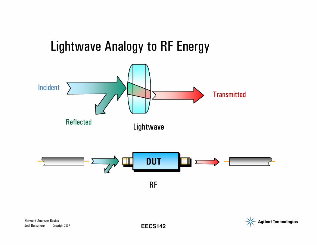
Incident
Reflected
Transmitted
Lightwave
DUT
Lightwave Analogy to RF Energy
Network Analyzer Basics
Joel Dunsmore Copyright 2007 EECS142
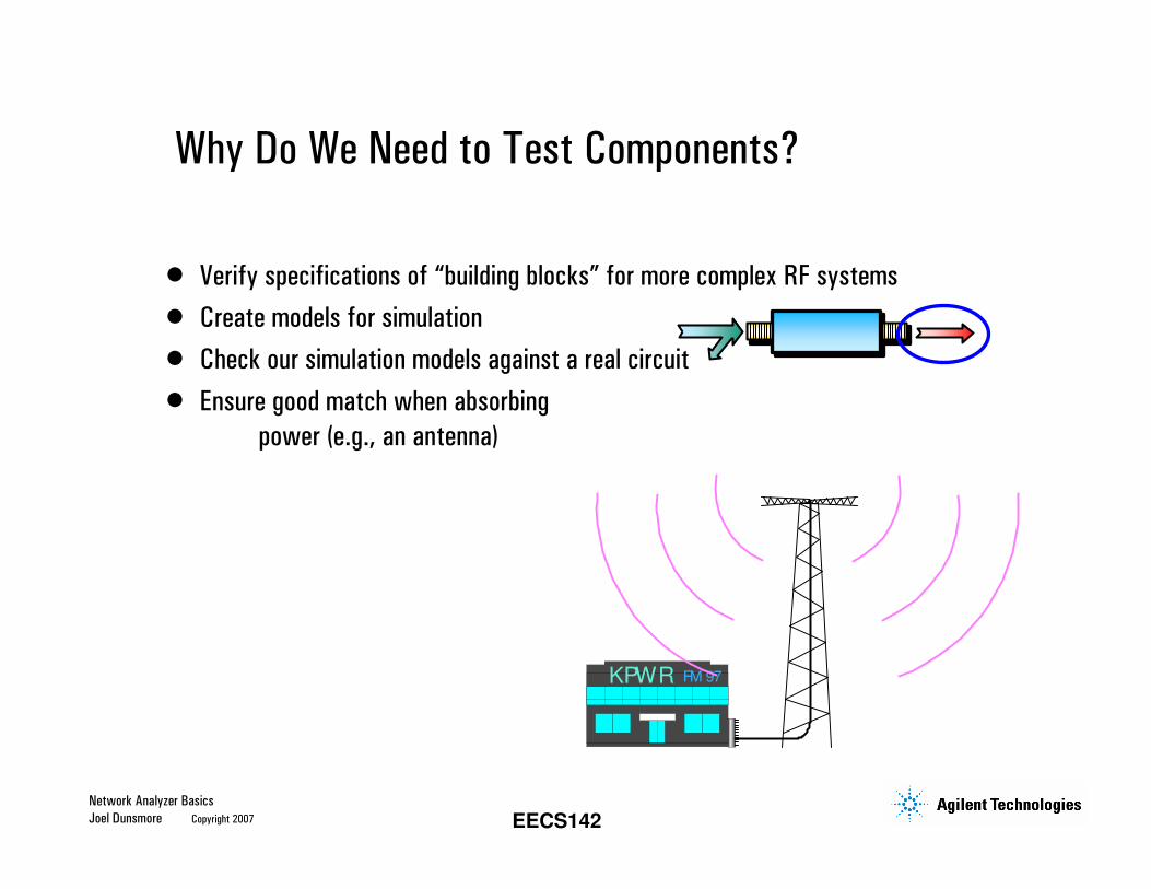
• Verify specifications of “building blocks” for more complex RF systems
• Create models for simulation
• Check our simulation models against a real circuit
• Ensure good match when absorbing
power (e.g., an antenna)
Why Do We Need to Test Components?
KPWR FM 97
Network Analyzer Basics
Joel Dunsmore Copyright 2007 EECS142
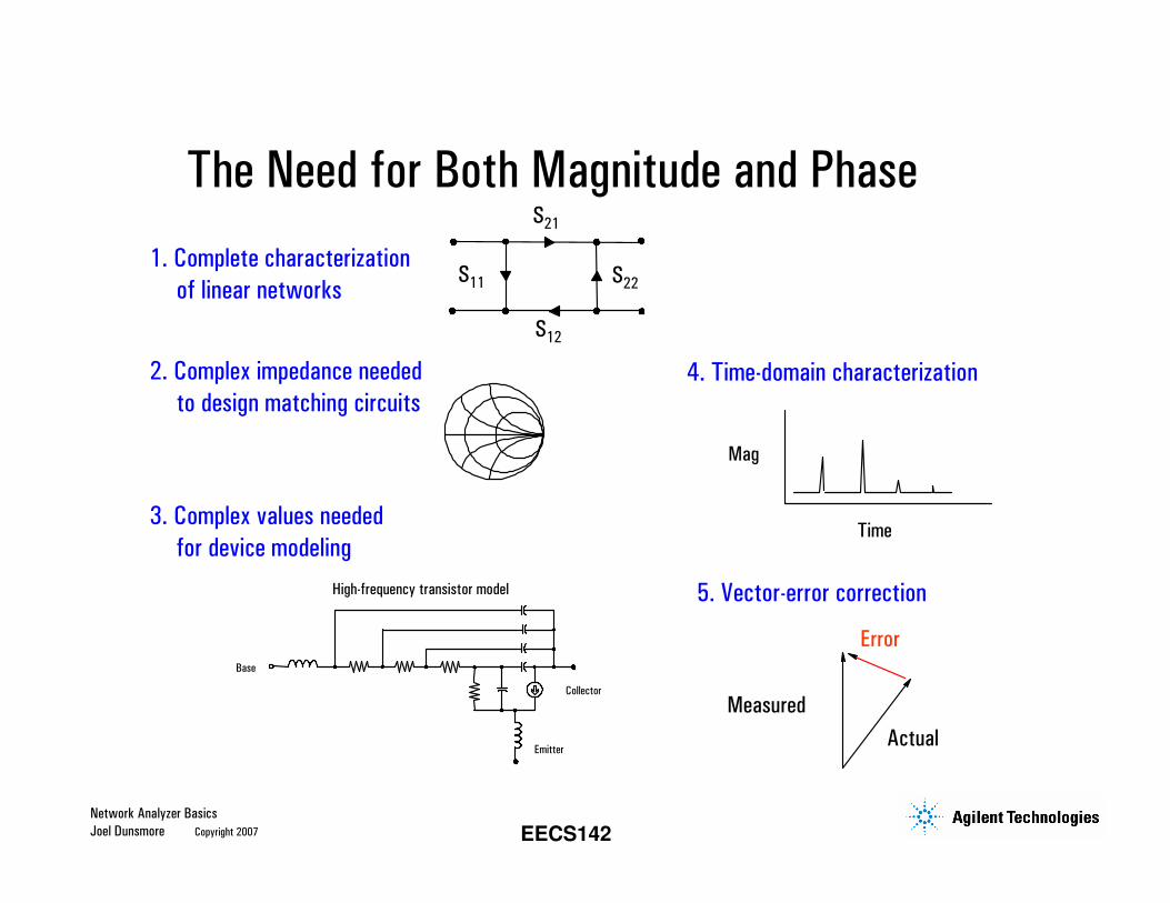
4. Time-domain characterization
Mag
Time
5. Vector-error correction
Error
Measured
Actual
2. Complex impedance needed
to design matching circuits
3. Complex values needed
for device modeling
1. Complete characterization
of linear networks
High-frequency transistor model
Collector
Base
Emitter
S21
S12
S11 S22
The Need for Both Magnitude and Phase
Network Analyzer Basics
Joel Dunsmore Copyright 2007 EECS142
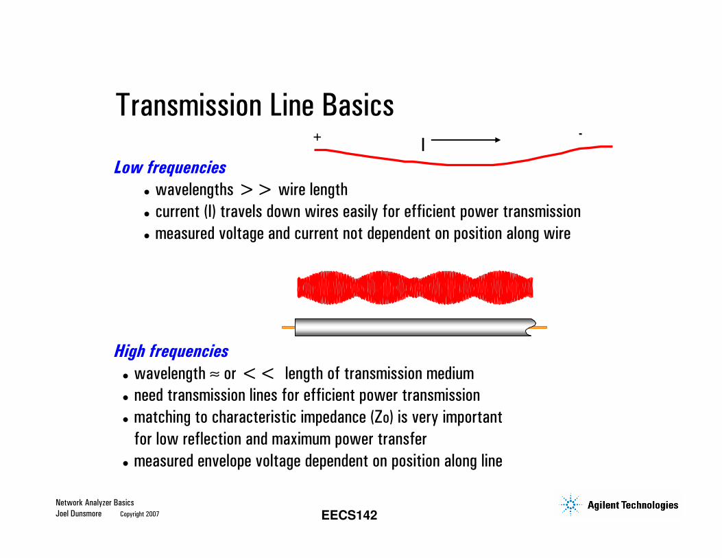
Low frequencies
wavelengths >> wire length
current (I) travels down wires easily for efficient power transmission
measured voltage and current not dependent on position along wire
High frequencies
wavelength ≈ or << length of transmission medium
need transmission lines for efficient power transmission
matching to characteristic impedance (Zo) is very important
for low reflection and maximum power transfer
measured envelope voltage dependent on position along line
I+ -
Transmission Line Basics
Network Analyzer Basics
Joel Dunsmore Copyright 2007 EECS142
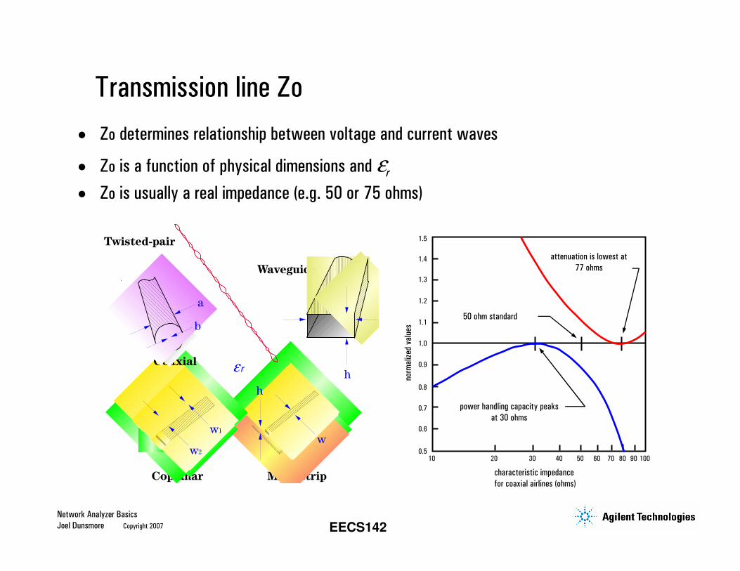
Transmission line Zo
• Zo determines relationship between voltage and current waves
• Zo is a function of physical dimensions and εr
• Zo is usually a real impedance (e.g. 50 or 75 ohms)
characteristic impedance
for coaxial airlines (ohms)
10 20 30 40 50 60 70 80 90 100
1.0
0.8
0.7
0.6
0.5
0.9
1.5
1.4
1.3
1.2
1.1
norm
aliz
ed v
alue
s
50 ohm standard
attenuation is lowest at
77 ohms
power handling capacity peaks
at 30 ohms
Microstrip
h
w
Coplanar
w1
w2
ε r
Waveguide
Twisted-pair
Coaxial
b
a
h
Network Analyzer Basics
Joel Dunsmore Copyright 2007 EECS142
RS
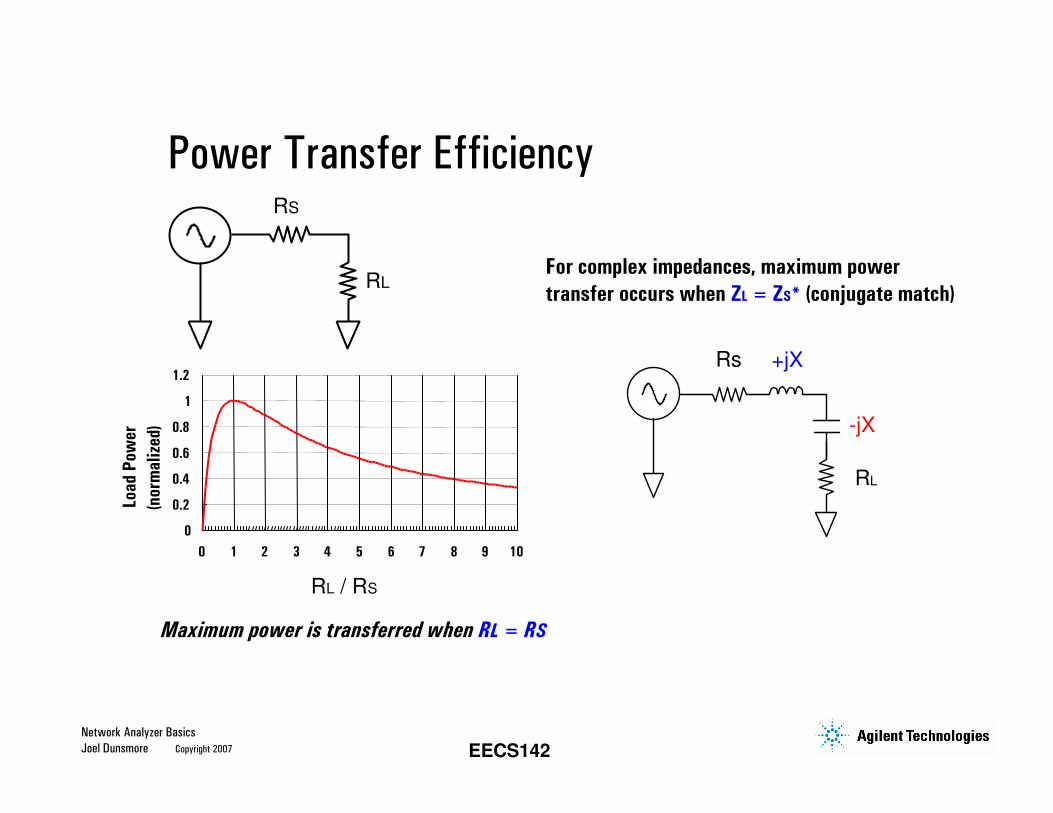
RLFor complex impedances, maximum power
transfer occurs when ZL = ZS* (conjugate match)
Maximum power is transferred when RL = RS
RL / RS
0
0.2
0.4
0.6
0.8
1
1.2
0 1 2 3 4 5 6 7 8 9 10
Load Pow
er
(normalized)
Rs
RL
+jX
-jX
Power Transfer Efficiency
Network Analyzer Basics
Joel Dunsmore Copyright 2007 EECS142
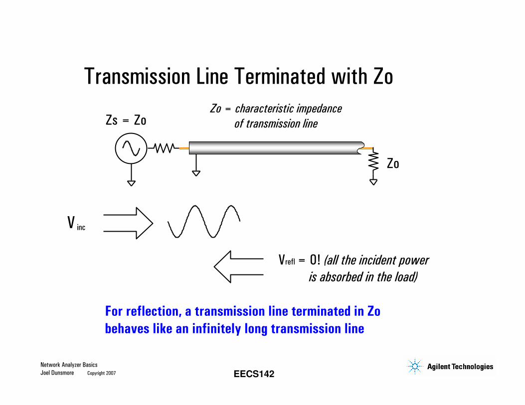
For reflection, a transmission line terminated in Zo
behaves like an infinitely long transmission line
Zs = Zo
Zo
Vrefl = 0! (all the incident power
is absorbed in the load)
V inc
Zo = characteristic impedance
of transmission line
Transmission Line Terminated with Zo
Network Analyzer Basics
Joel Dunsmore Copyright 2007 EECS142
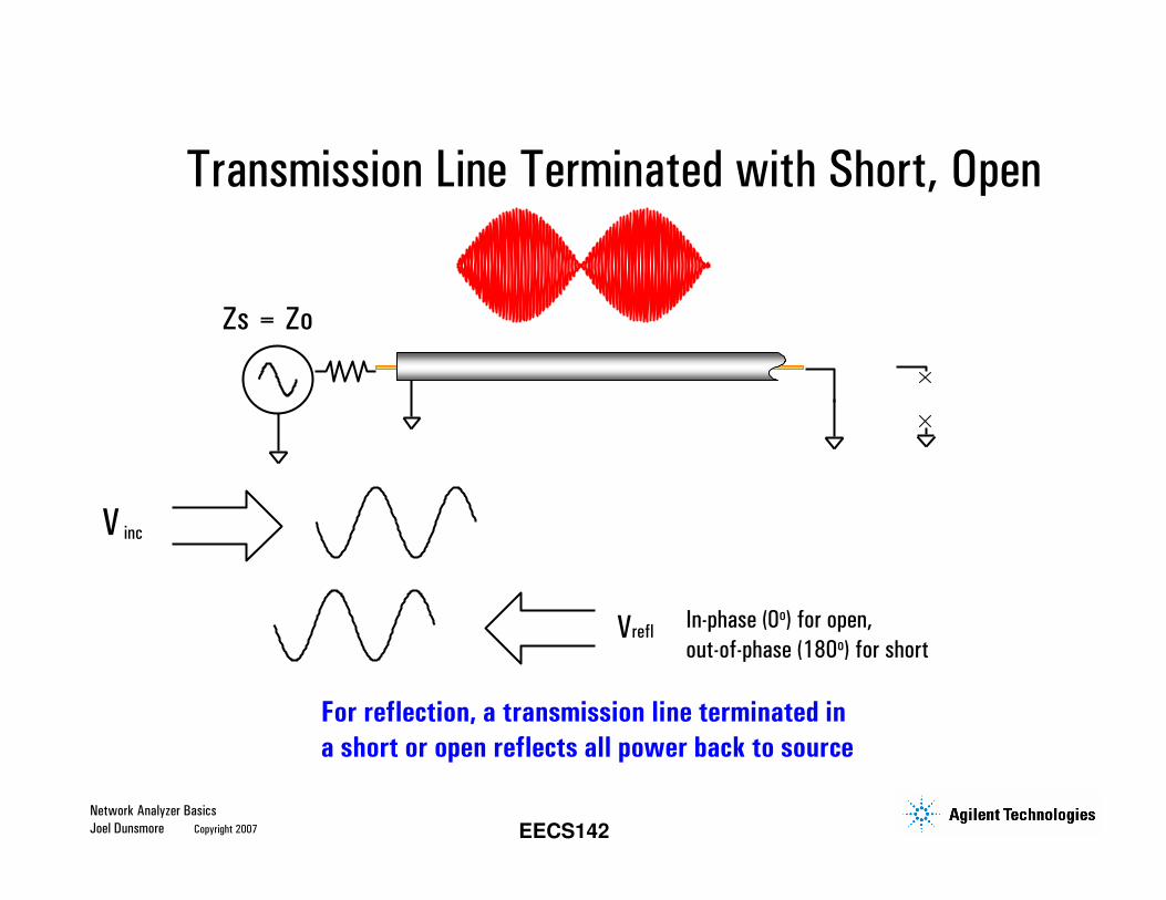
Zs = Zo
Vrefl
V inc
For reflection, a transmission line terminated in
a short or open reflects all power back to source
In-phase (0o) for open,
out-of-phase (180o) for short
Transmission Line Terminated with Short, Open
Network Analyzer Basics
Joel Dunsmore Copyright 2007 EECS142
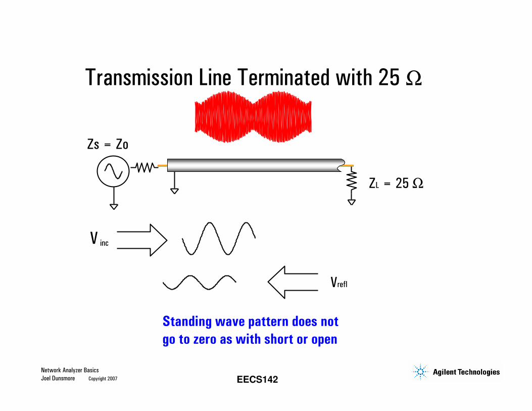
Vrefl
Standing wave pattern does not
go to zero as with short or open
Zs = Zo
ZL = 25 Ω
V inc
Transmission Line Terminated with 25 Ω
Network Analyzer Basics
Joel Dunsmore Copyright 2007 EECS142
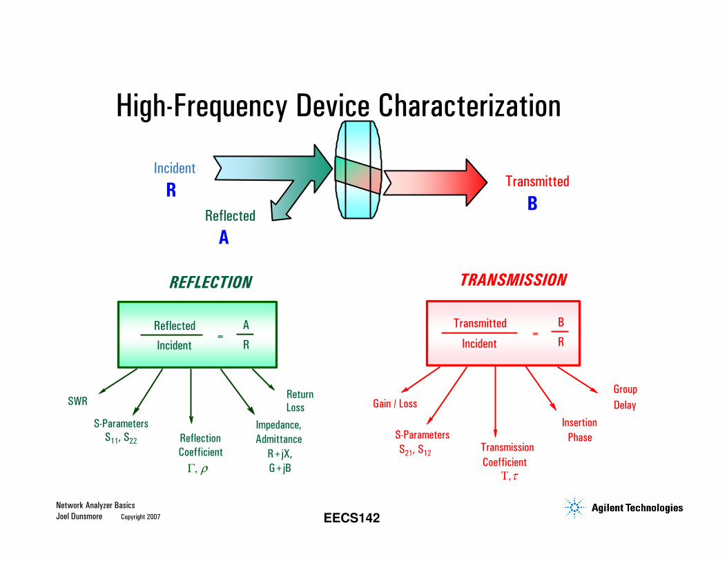
Transmitted
Incident
TRANSMISSION
Gain / Loss
S-Parameters
S21, S12
Group
Delay
Transmission
Coefficient
Insertion
Phase
Reflected
Incident
REFLECTION
SWR
S-Parameters
S11, S22 Reflection
Coefficient
Impedance,
Admittance
R+jX,
G+jB
Return
Loss
Γ, ρΤ,τ
Incident
Reflected
TransmittedR
B
A
A
R=
B
R=
High-Frequency Device Characterization
Network Analyzer Basics
Joel Dunsmore Copyright 2007 EECS142
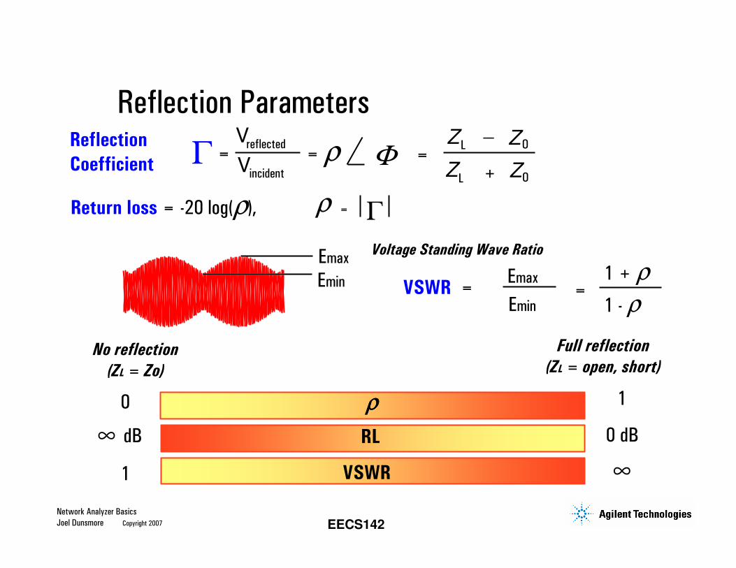
∞ dB
No reflection
(ZL = Zo)
ρρρρ
RL
VSWR
0 1
Full reflection
(ZL = open, short)
0 dB
1 ∞
=ZL − ZO
ZL + OZ
Reflection
Coefficient=
Vreflected
Vincident
= ρ ΦΓ
=ρ ΓReturn loss = -20 log(ρ),
Voltage Standing Wave Ratio
VSWR = Emax
Emin=
1 + ρ
1 - ρ
Emax
Emin
Reflection Parameters
Network Analyzer Basics
Joel Dunsmore Copyright 2007 EECS142
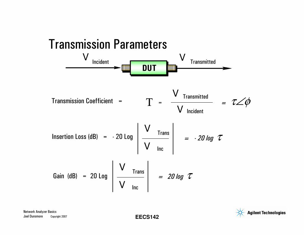
VTransmitted
VIncident
Transmission Coefficient = Τ =
V Transmitted
V Incident
= τ∠φ
DUT
Gain (dB) = 20 Log V
Trans
V Inc
= 20 log τ
Insertion Loss (dB) = - 20 Log V
Trans
V Inc
= - 20 log τ
Transmission Parameters
Network Analyzer Basics
Joel Dunsmore Copyright 2007 EECS142
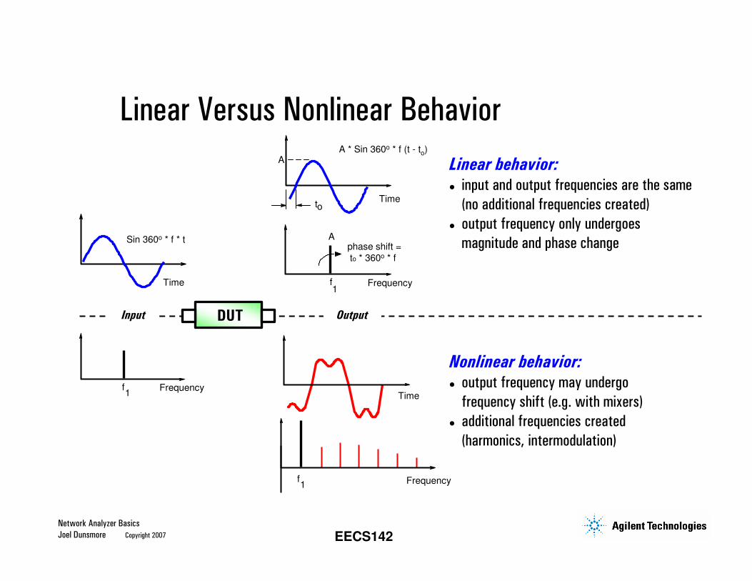
Linear behavior: input and output frequencies are the same
(no additional frequencies created)
output frequency only undergoes
magnitude and phase change
Frequencyf1
Time
Sin 360o * f * t
Frequency
Aphase shift =
to * 360o * f
1f
DUT
Time
A
to
A * Sin 360o * f (t - to)
Input Output
Time
Nonlinear behavior: output frequency may undergo
frequency shift (e.g. with mixers)
additional frequencies created
(harmonics, intermodulation)
Frequencyf1
Linear Versus Nonlinear Behavior
Network Analyzer Basics
Joel Dunsmore Copyright 2007 EECS142
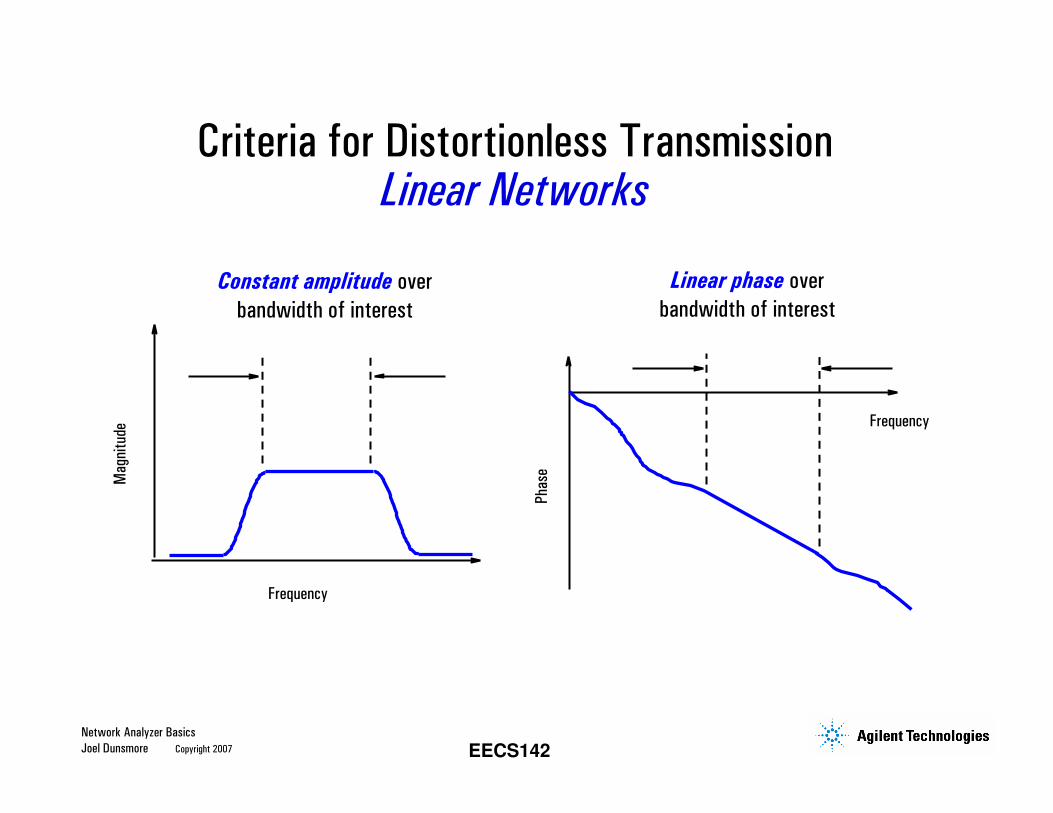
Constant amplitude over
bandwidth of interest
Mag
nitu
de
Pha
se
Frequency
Frequency
Linear phase over
bandwidth of interest
Criteria for Distortionless TransmissionLinear Networks
Network Analyzer Basics
Joel Dunsmore Copyright 2007 EECS142
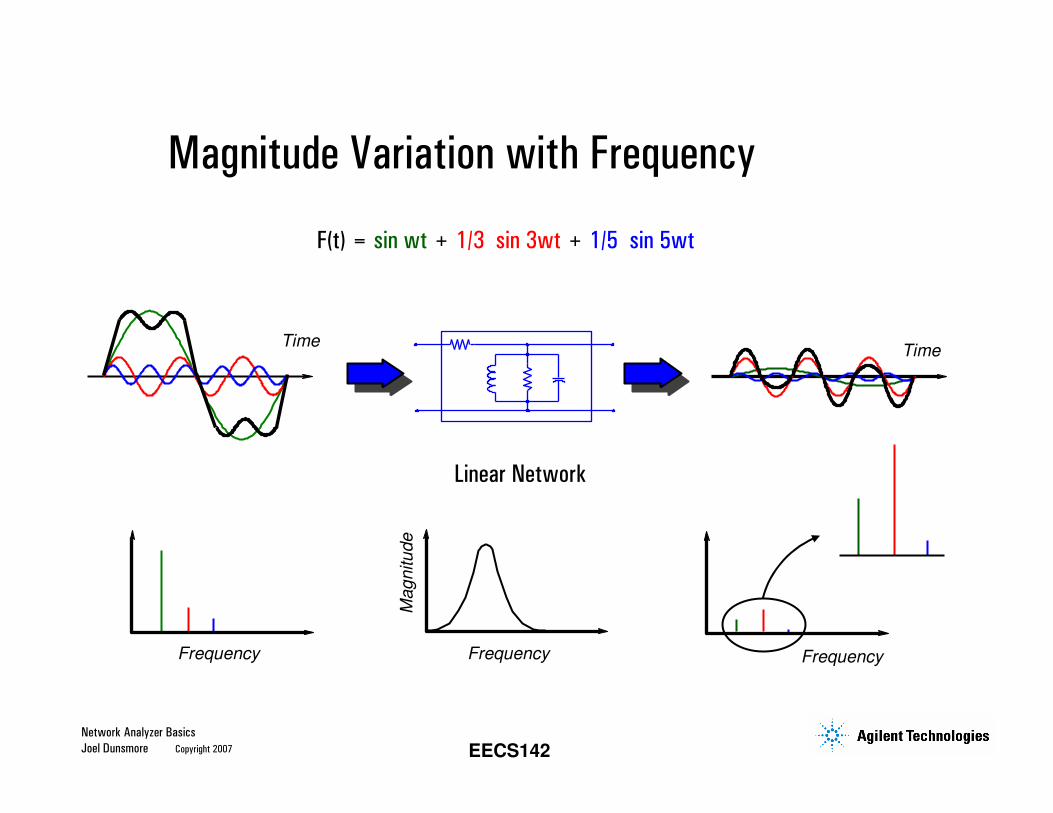
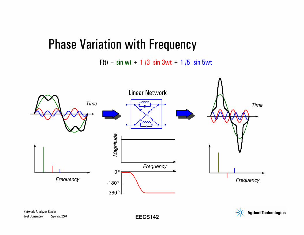
F(t) = sin wt + 1/3 sin 3wt + 1/5 sin 5wt
Time
Linear Network
Frequency Frequency Frequency
Mag
nitu
de
Time
Magnitude Variation with Frequency
Network Analyzer Basics
Joel Dunsmore Copyright 2007 EECS142
Frequency
Mag
nitu
de
Linear Network
Frequency
Frequency
Time
0
-180
-360
°
°
°
Time
F(t) = sin wt + 1 /3 sin 3wt + 1 /5 sin 5wt
Phase Variation with Frequency
Network Analyzer Basics
Joel Dunsmore Copyright 2007 EECS142
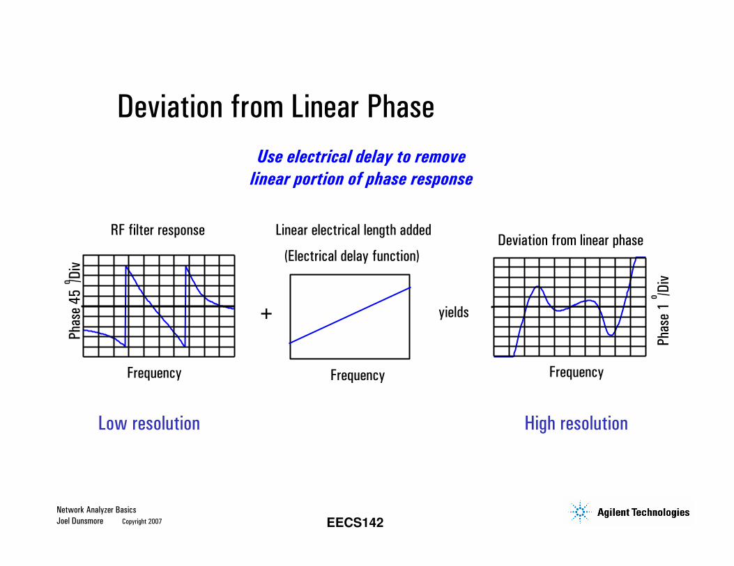
Use electrical delay to remove
linear portion of phase response
Linear electrical length added
+ yields
Frequency
(Electrical delay function)
Frequency
RF filter responseDeviation from linear phase
Pha
se 1
/D
ivo
Pha
se 4
5 /
Div
o
Frequency
Low resolution High resolution
Deviation from Linear Phase
Network Analyzer Basics
Joel Dunsmore Copyright 2007 EECS142
in radians
in radians/sec
in degrees
f in Hertz (ω = 2 π f)
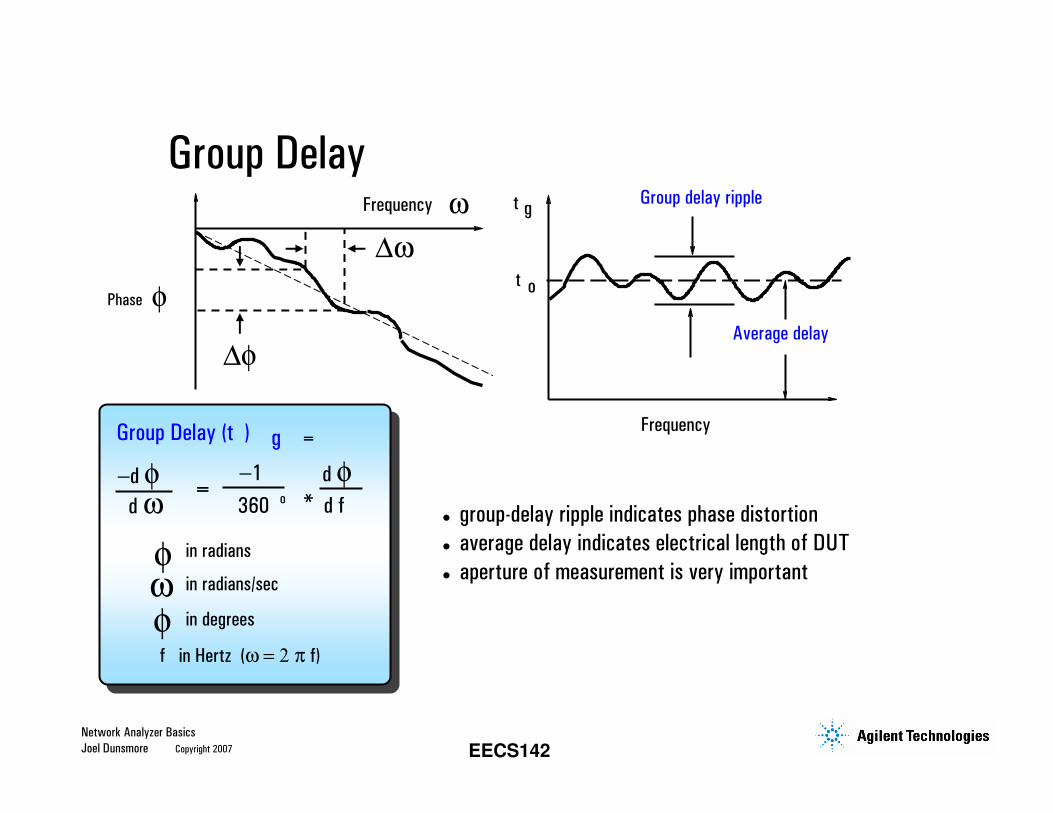
φωφ
Group Delay (t ) g =
−d φd ω
=−1
360 o
d φd f*
Frequency
Group delay ripple
Average delay
t o
t g
Phase φ
∆φ
Frequency
∆ω
ω
group-delay ripple indicates phase distortion
average delay indicates electrical length of DUT
aperture of measurement is very important
Group Delay
Network Analyzer Basics
Joel Dunsmore Copyright 2007 EECS142
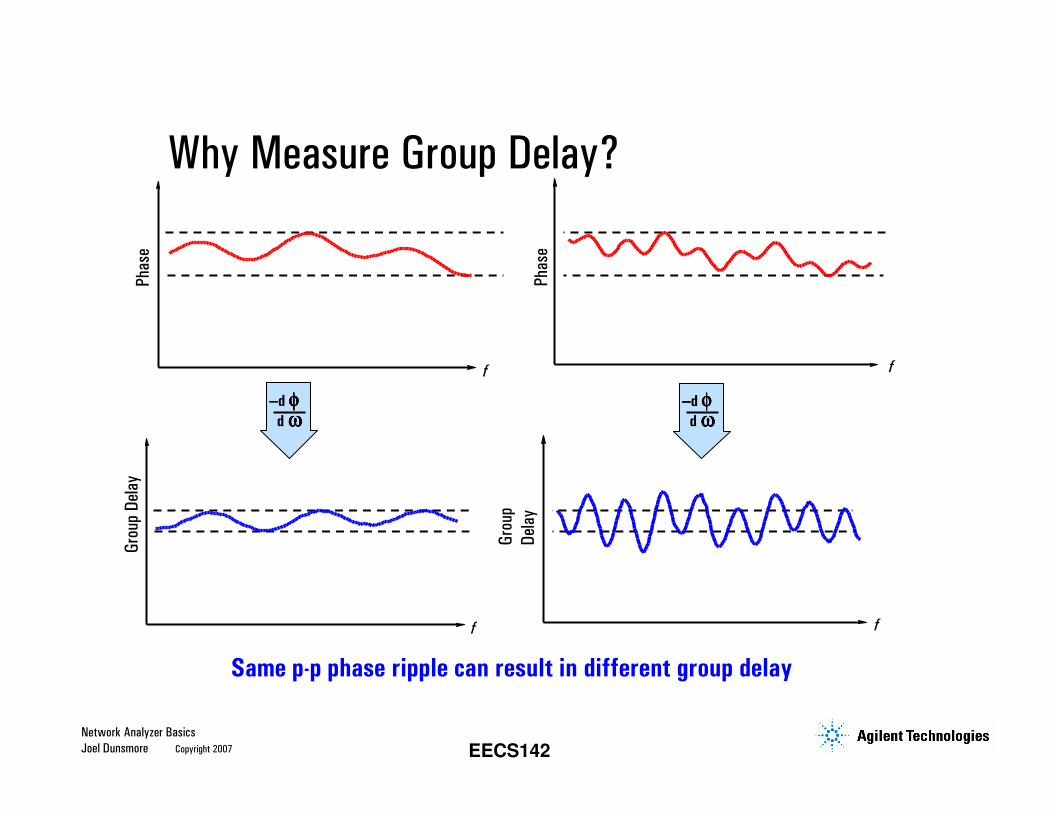
Same p-p phase ripple can result in different group delay
Pha
se
Pha
se
Gro
up D
elay
Gro
up
Del
ay
−−−−d φφφφd ωωωω
−−−−d φφφφd ωωωω
f
f
f
f
Why Measure Group Delay?
Network Analyzer Basics
Joel Dunsmore Copyright 2007 EECS142
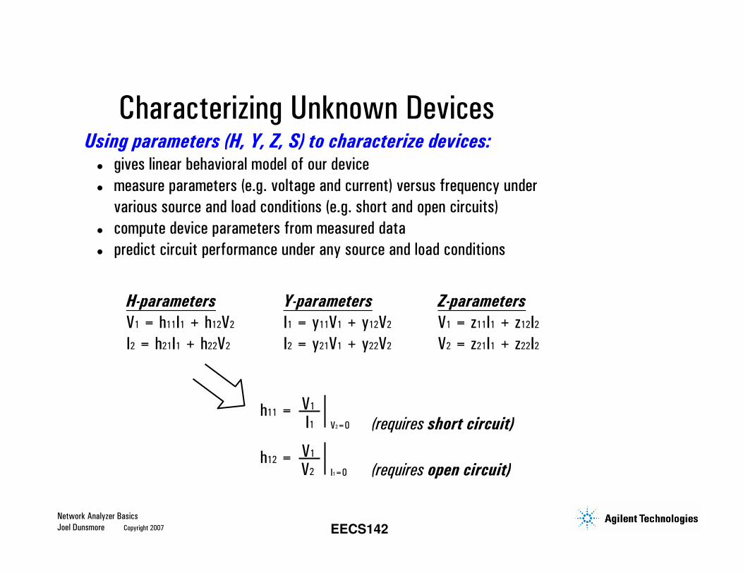
Using parameters (H, Y, Z, S) to characterize devices: gives linear behavioral model of our device
measure parameters (e.g. voltage and current) versus frequency under
various source and load conditions (e.g. short and open circuits)
compute device parameters from measured data
predict circuit performance under any source and load conditions
H-parameters
V1 = h11I1 + h12V2
I2 = h21I1 + h22V2
Y-parameters
I1 = y11V1 + y12V2
I2 = y21V1 + y22V2
Z-parameters
V1 = z11I1 + z12I2
V2 = z21I1 + z22I2
h11 = V1
I1 V2=0
h12 = V1
V2 I1=0
(requires short circuit)
(requires open circuit)
Characterizing Unknown Devices
Network Analyzer Basics
Joel Dunsmore Copyright 2007 EECS142
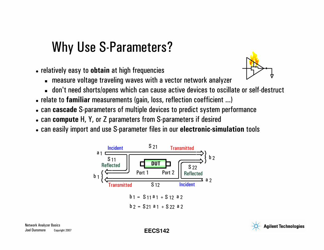
relatively easy to obtain at high frequencies
measure voltage traveling waves with a vector network analyzer
don't need shorts/opens which can cause active devices to oscillate or self-destruct
relate to familiar measurements (gain, loss, reflection coefficient ...)
can cascade S-parameters of multiple devices to predict system performance
can compute H, Y, or Z parameters from S-parameters if desired
can easily import and use S-parameter files in our electronic-simulation tools
Incident TransmittedS 21
S 11Reflected S 22
Reflected
Transmitted Incident
b 1
a 1b 2
a 2S 12
DUT
b 1 = S 11 a 1 + S 12 a 2
b 2 = S 21 a 1 + S 22 a 2
Port 1 Port 2
Why Use S-Parameters?
Network Analyzer Basics
Joel Dunsmore Copyright 2007 EECS142
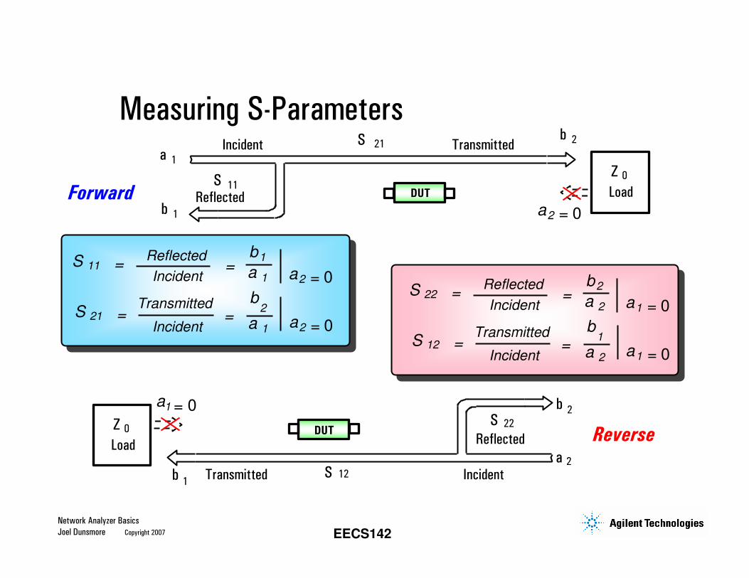
S 11 =Reflected
Incident=
b1
a 1 a2 = 0
S 21 =Transmitted
Incident=
b2
a 1 a2 = 0
S 22 =Reflected
Incident=
b2
a 2 a1 = 0
S 12 =Transmitted
Incident=
b1
a 2 a1 = 0
Incident TransmittedS 21
S 11
Reflectedb 1
a 1
b 2
Z 0
Load
a2 = 0
DUTForward
IncidentTransmitted S 12
S 22
Reflected
b 2
a 2
b
a1 = 0
DUTZ 0
LoadReverse
1
Measuring S-Parameters
Network Analyzer Basics
Joel Dunsmore Copyright 2007 EECS142
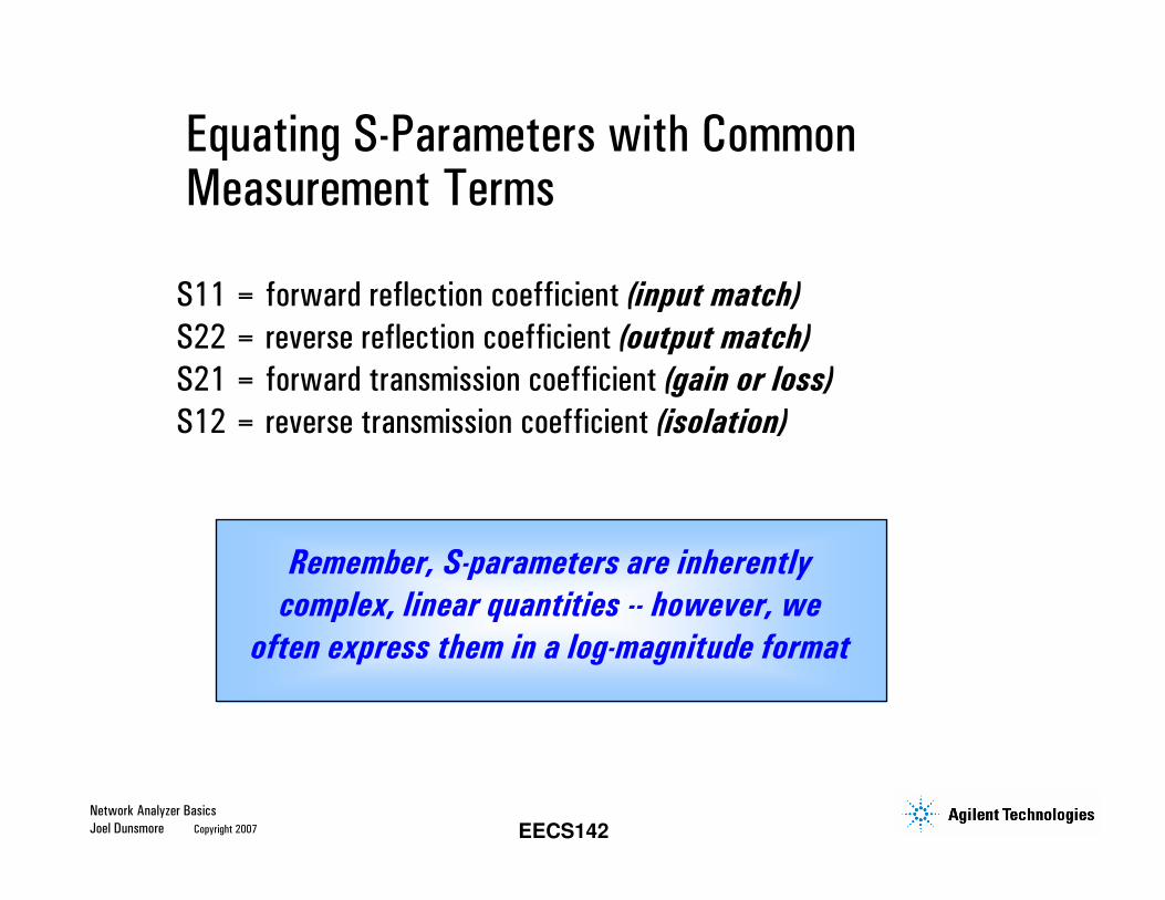
S11 = forward reflection coefficient (input match)
S22 = reverse reflection coefficient (output match)
S21 = forward transmission coefficient (gain or loss)
S12 = reverse transmission coefficient (isolation)
Remember, S-parameters are inherently
complex, linear quantities -- however, we
often express them in a log-magnitude format
Equating S-Parameters with Common Measurement Terms
Network Analyzer Basics
Joel Dunsmore Copyright 2007 EECS142
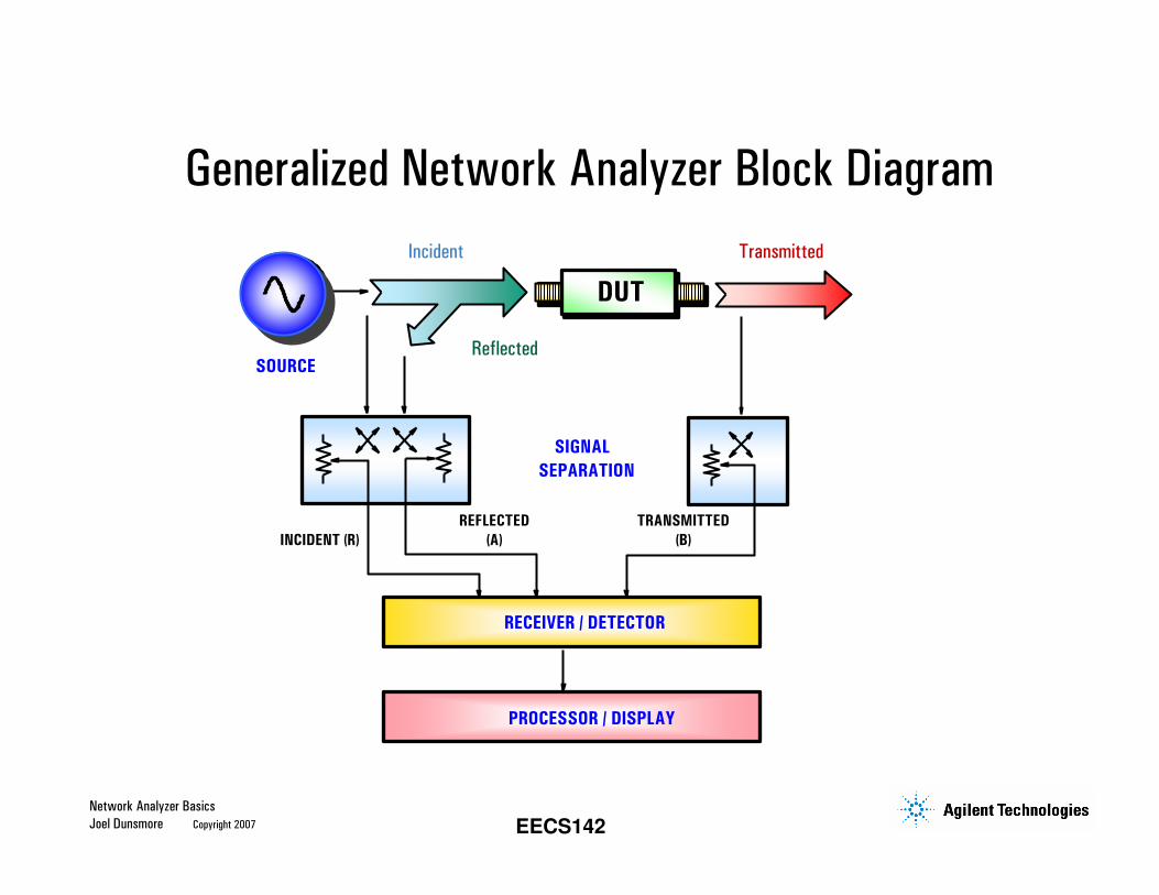
RECEIVER / DETECTOR
PROCESSOR / DISPLAY
REFLECTED
(A)
TRANSMITTED
(B)INCIDENT (R)
SIGNAL
SEPARATION
SOURCE
Incident
Reflected
Transmitted
DUT
Generalized Network Analyzer Block Diagram
Network Analyzer Basics
Joel Dunsmore Copyright 2007 EECS142
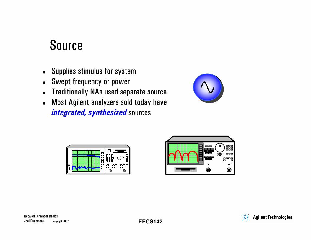
Supplies stimulus for system
Swept frequency or power
Traditionally NAs used separate source
Most Agilent analyzers sold today have
integrated, synthesized sources
Source
Network Analyzer Basics
Joel Dunsmore Copyright 2007 EECS142
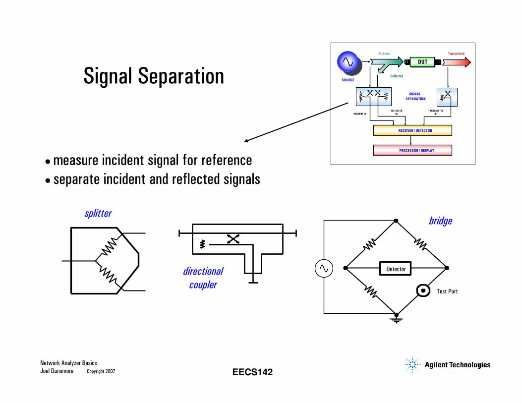
Test Port
Detectordirectional
coupler
splitterbridge
• measure incident signal for reference
• separate incident and reflected signals
RECEIVER / DETECTOR
PROCESSOR / DISPLAY
REFLECTED
(A)
TRANSMITTED
(B)INCIDENT (R)
SIGNAL
SEPARATION
SOURCE
Incident
Reflected
Transmitted
DUT
Signal Separation
Network Analyzer Basics
Joel Dunsmore Copyright 2007 EECS142
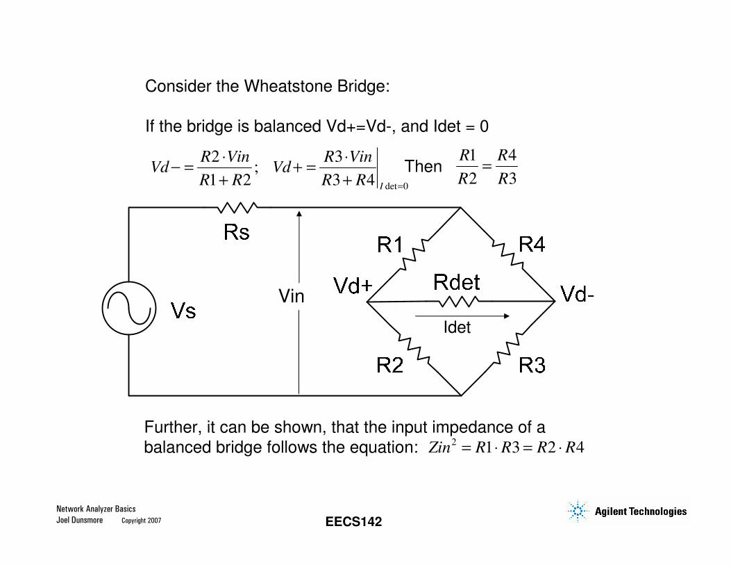
Consider the Wheatstone Bridge:
If the bridge is balanced Vd+=Vd-, and Idet = 0
1 4
2 3
R R
R R=
det 0
2 3;
1 2 3 4I
R Vin R VinVd Vd
R R R R =
⋅ ⋅− = + =
+ +Then
Further, it can be shown, that the input impedance of a
balanced bridge follows the equation: 21 3 2 4Zin R R R R= ⋅ = ⋅
Idet
Vin
Network Analyzer Basics
Joel Dunsmore Copyright 2007 EECS142
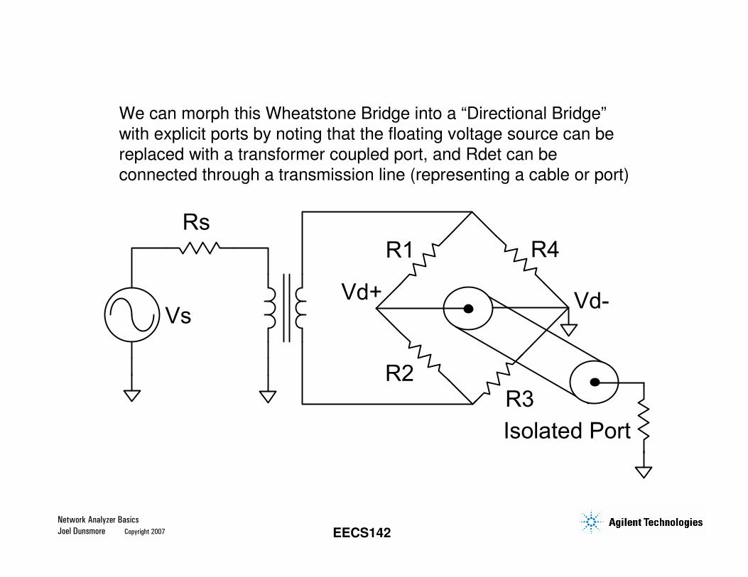
We can morph this Wheatstone Bridge into a “Directional Bridge”
with explicit ports by noting that the floating voltage source can be
replaced with a transformer coupled port, and Rdet can be
connected through a transmission line (representing a cable or port)
Rs
R4R1
R3R2
Isolated Port
Vd-Vd+Vs
Network Analyzer Basics
Joel Dunsmore Copyright 2007 EECS142
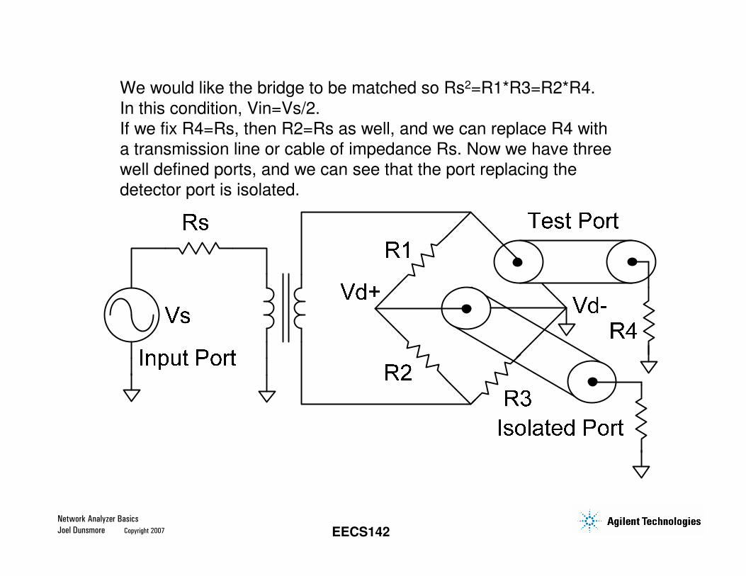
We would like the bridge to be matched so Rs2=R1*R3=R2*R4.
In this condition, Vin=Vs/2.
If we fix R4=Rs, then R2=Rs as well, and we can replace R4 with
a transmission line or cable of impedance Rs. Now we have three
well defined ports, and we can see that the port replacing the
detector port is isolated.
Network Analyzer Basics
Joel Dunsmore Copyright 2007 EECS142
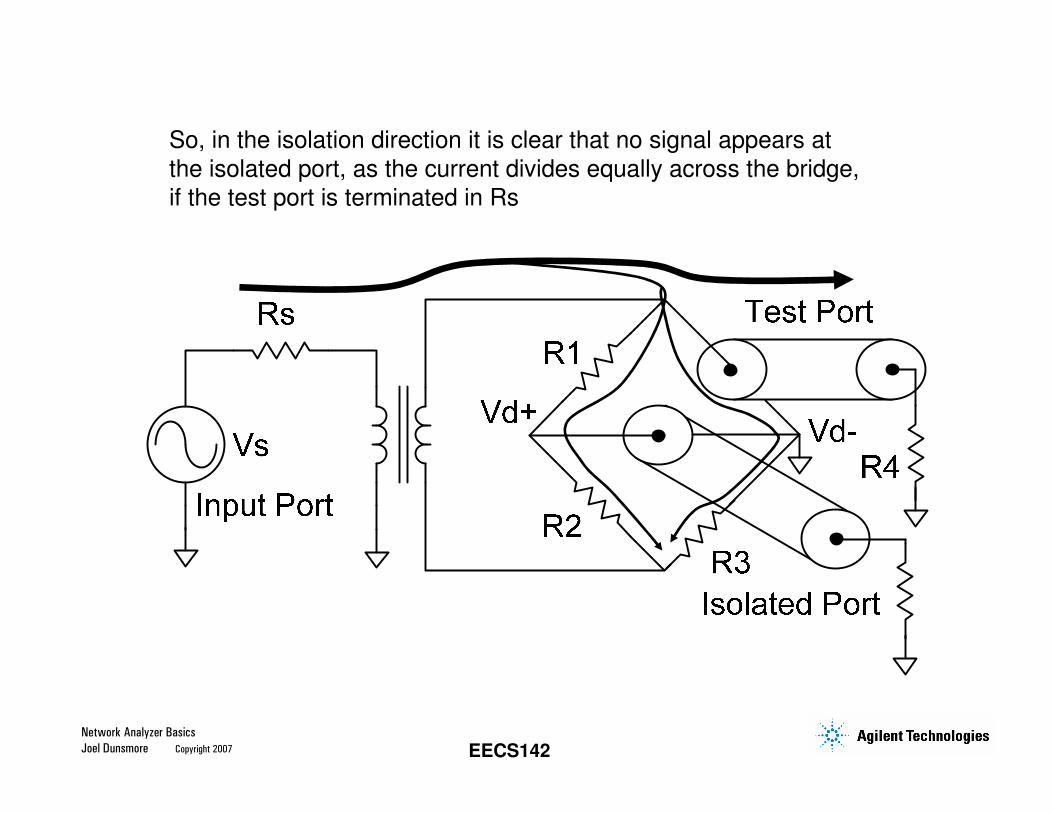
So, in the isolation direction it is clear that no signal appears at
the isolated port, as the current divides equally across the bridge,
if the test port is terminated in Rs
Network Analyzer Basics
Joel Dunsmore Copyright 2007 EECS142
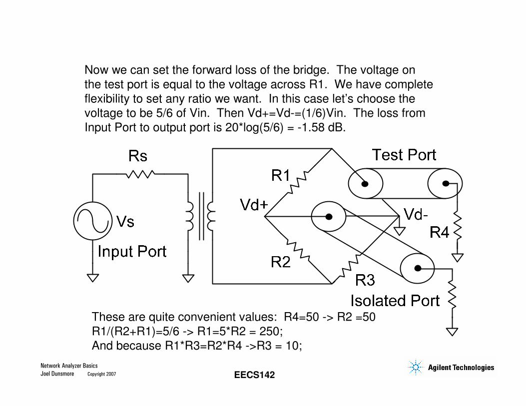
Now we can set the forward loss of the bridge. The voltage on
the test port is equal to the voltage across R1. We have complete
flexibility to set any ratio we want. In this case let’s choose the
voltage to be 5/6 of Vin. Then Vd+=Vd-=(1/6)Vin. The loss from
Input Port to output port is 20*log(5/6) = -1.58 dB.
These are quite convenient values: R4=50 -> R2 =50
R1/(R2+R1)=5/6 -> R1=5*R2 = 250;
And because R1*R3=R2*R4 ->R3 = 10;
Network Analyzer Basics
Joel Dunsmore Copyright 2007 EECS142
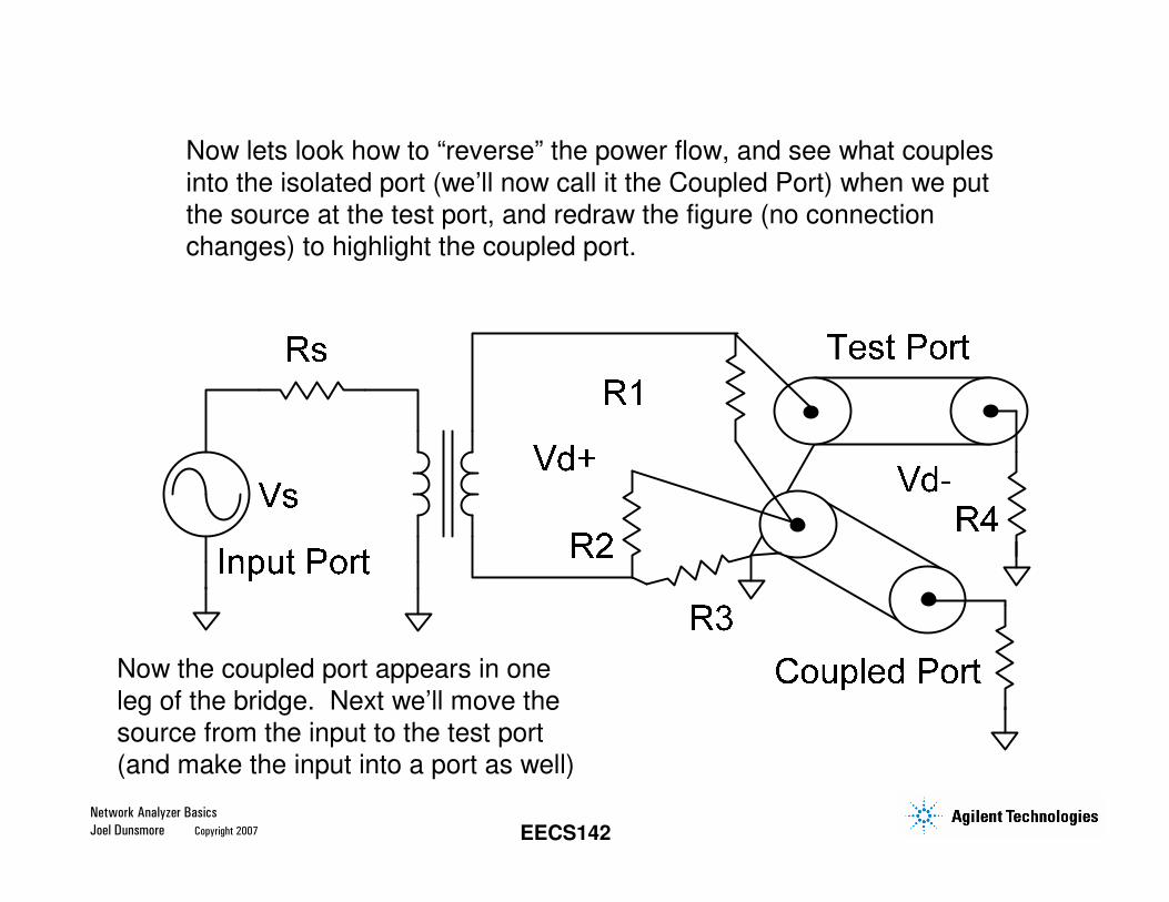
Now lets look how to “reverse” the power flow, and see what couples
into the isolated port (we’ll now call it the Coupled Port) when we put
the source at the test port, and redraw the figure (no connection
changes) to highlight the coupled port.
Now the coupled port appears in one
leg of the bridge. Next we’ll move the
source from the input to the test port
(and make the input into a port as well)
Network Analyzer Basics
Joel Dunsmore Copyright 2007 EECS142
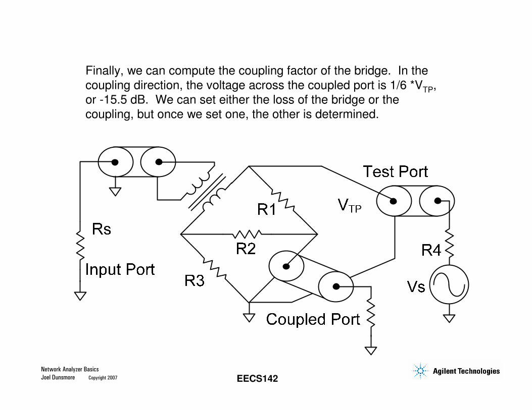
Finally, we can compute the coupling factor of the bridge. In the
coupling direction, the voltage across the coupled port is 1/6 *VTP,
or -15.5 dB. We can set either the loss of the bridge or the
coupling, but once we set one, the other is determined.
Network Analyzer Basics
Joel Dunsmore Copyright 2007 EECS142
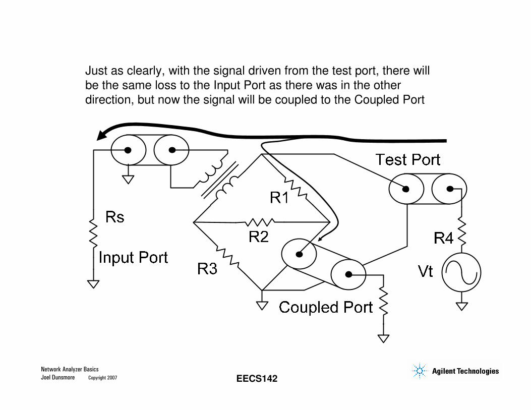
Just as clearly, with the signal driven from the test port, there will
be the same loss to the Input Port as there was in the other
direction, but now the signal will be coupled to the Coupled Port
Network Analyzer Basics
Joel Dunsmore Copyright 2007 EECS142
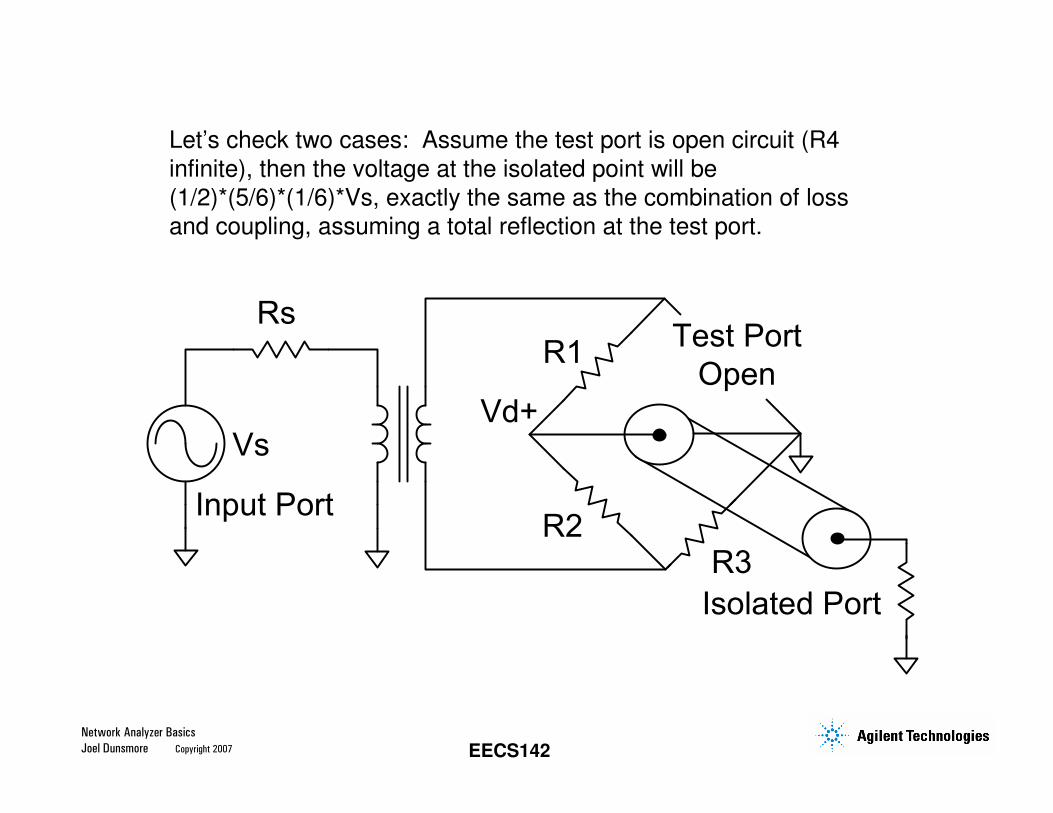
Let’s check two cases: Assume the test port is open circuit (R4
infinite), then the voltage at the isolated point will be
(1/2)*(5/6)*(1/6)*Vs, exactly the same as the combination of loss
and coupling, assuming a total reflection at the test port.
Rs
R1
R3R2
Vd+Vs
Test Port
Open
Isolated Port
Input Port
Network Analyzer Basics
Joel Dunsmore Copyright 2007 EECS142
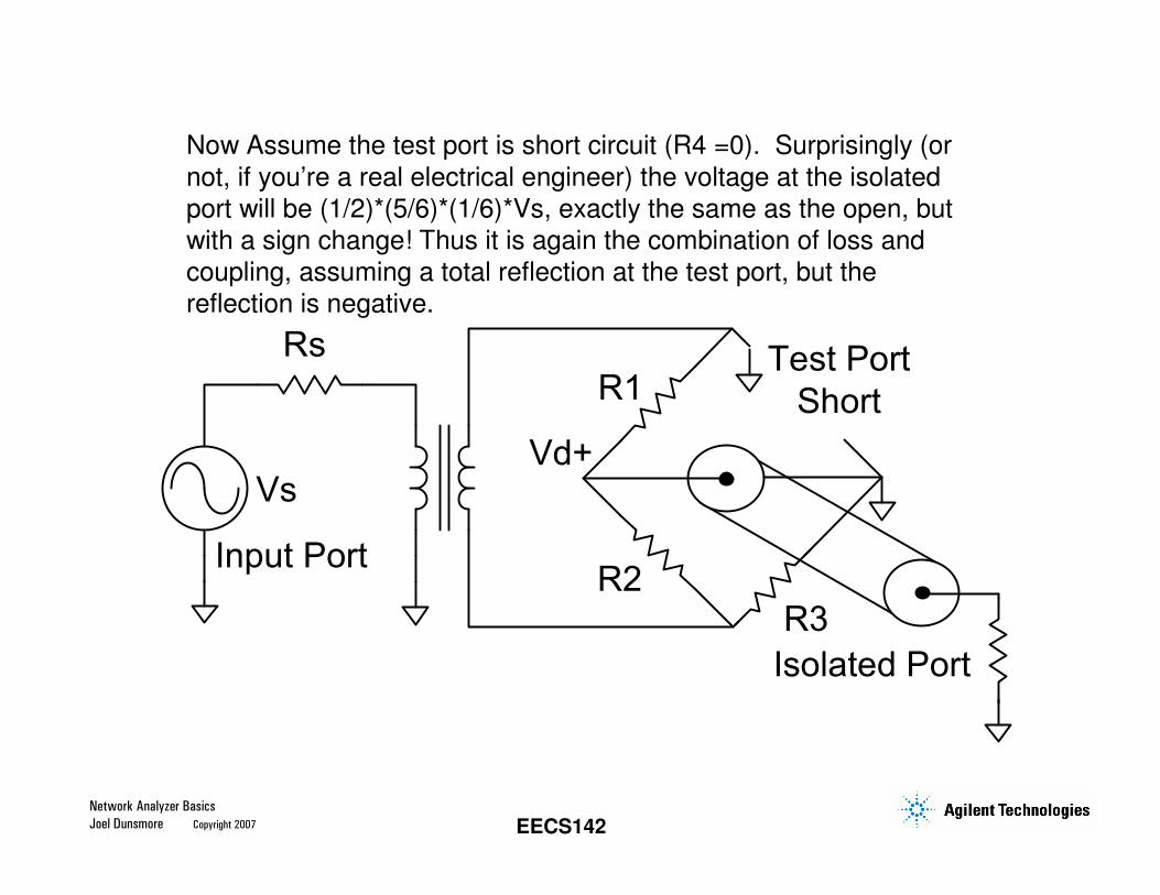
Now Assume the test port is short circuit (R4 =0). Surprisingly (or
not, if you’re a real electrical engineer) the voltage at the isolated
port will be (1/2)*(5/6)*(1/6)*Vs, exactly the same as the open, but
with a sign change! Thus it is again the combination of loss and
coupling, assuming a total reflection at the test port, but the
reflection is negative.
Rs
R1
R3R2
Vd+Vs
Test Port
Short
Isolated Port
Input Port
Network Analyzer Basics
Joel Dunsmore Copyright 2007 EECS142
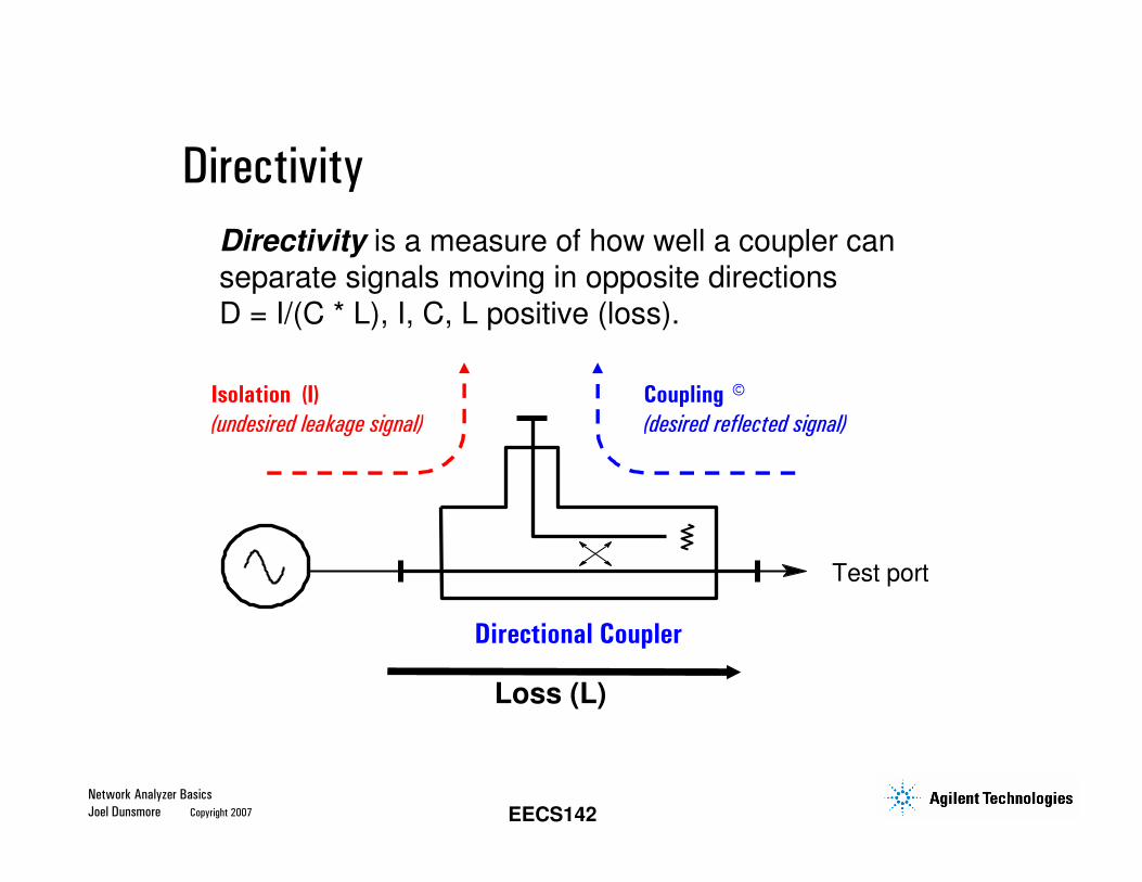
Directivity is a measure of how well a coupler can
separate signals moving in opposite directions
D = I/(C * L), I, C, L positive (loss).
Test port
Isolation (I)
(undesired leakage signal)
Coupling ©
(desired reflected signal)
Directional Coupler
Directivity
Loss (L)
Network Analyzer Basics
Joel Dunsmore Copyright 2007 EECS142
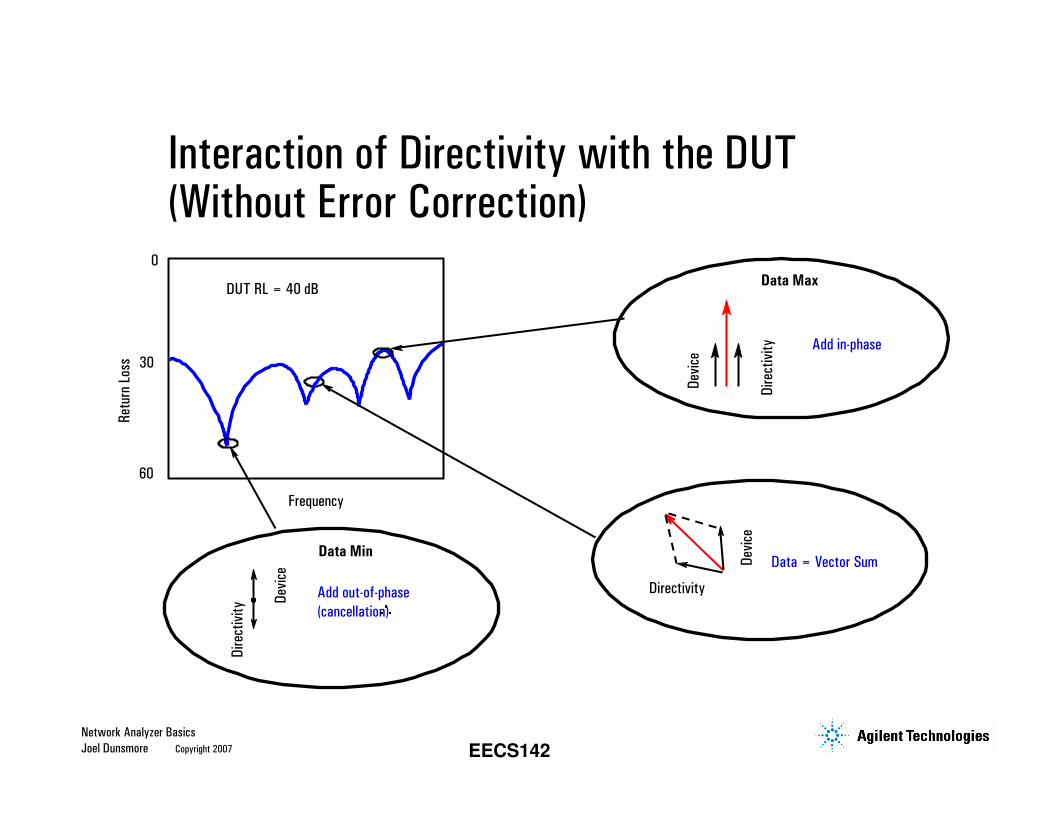
Data Max
Add in-phase
Dev
ice
Dir
ecti
vity
Ret
urn
Loss
Frequency
0
30
60
DUT RL = 40 dB
Add out-of-phase
(cancellation)
Dev
ice
Directivity
Data = Vector Sum
Dir
ecti
vity
Dev
ice
Data Min
Interaction of Directivity with the DUT (Without Error Correction)
Network Analyzer Basics
Joel Dunsmore Copyright 2007 EECS142
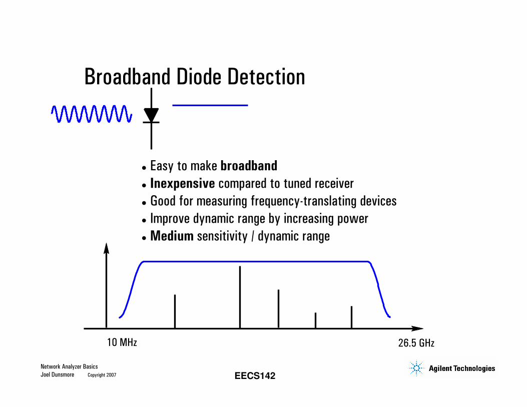
Easy to make broadband
Inexpensive compared to tuned receiver
Good for measuring frequency-translating devices
Improve dynamic range by increasing power
Medium sensitivity / dynamic range
10 MHz 26.5 GHz
Broadband Diode Detection
Network Analyzer Basics
Joel Dunsmore Copyright 2007 EECS142
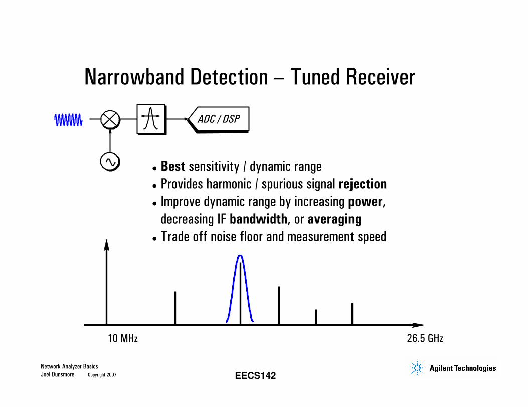
Best sensitivity / dynamic range
Provides harmonic / spurious signal rejection
Improve dynamic range by increasing power,
decreasing IF bandwidth, or averaging
Trade off noise floor and measurement speed
10 MHz 26.5 GHz
ADC / DSP
Narrowband Detection – Tuned Receiver
Network Analyzer Basics
Joel Dunsmore Copyright 2007 EECS142
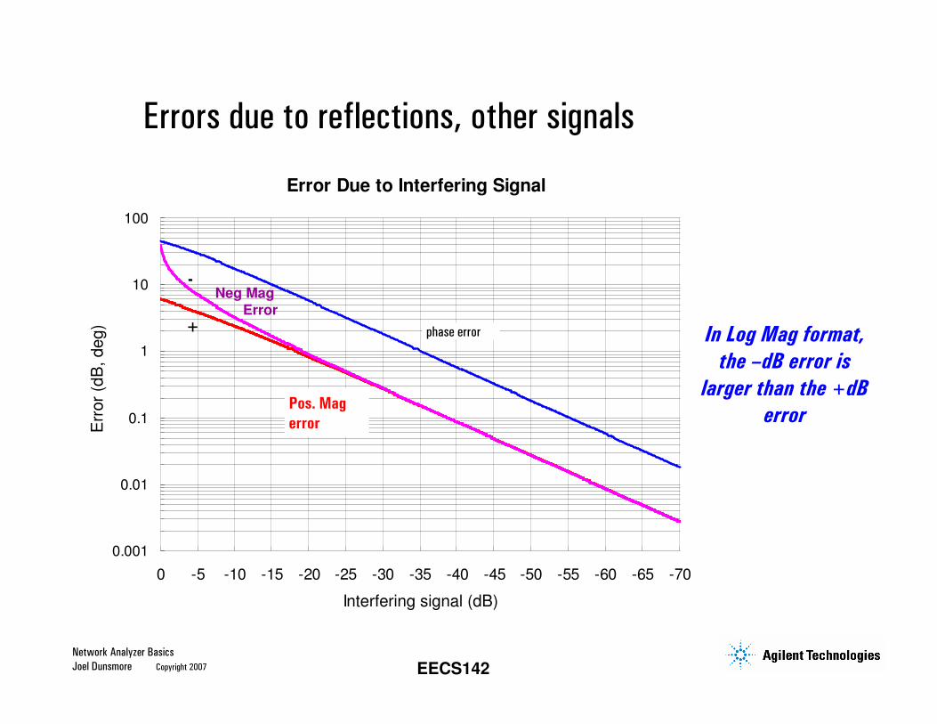
Error Due to Interfering Signal
0.001
0.01
0.1
1
10
100
0 -5 -10 -15 -20 -25 -30 -35 -40 -45 -50 -55 -60 -65 -70
Interfering signal (dB)
Err
or
(dB
, d
eg
) phase error
Pos. Mag
error
+
-
Errors due to reflections, other signals
In Log Mag format,
the –dB error is
larger than the +dB
error
Neg MagError
Network Analyzer Basics
Joel Dunsmore Copyright 2007 EECS142
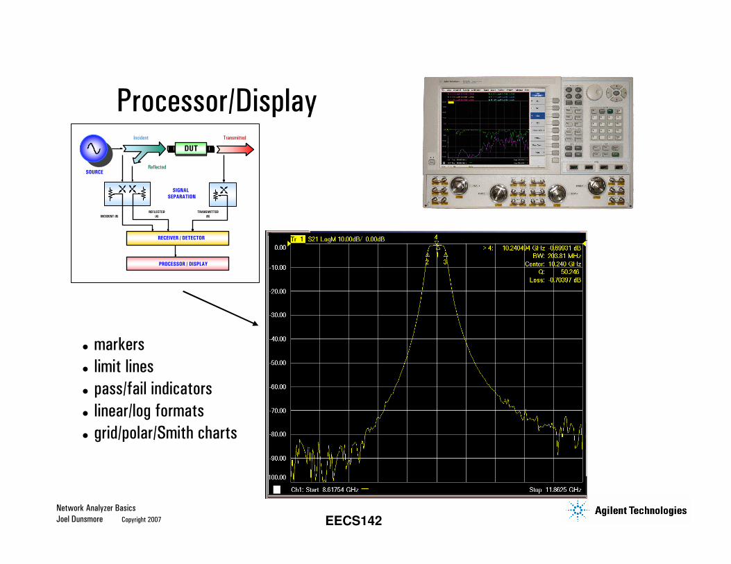
RECEIVER / DETECTOR
PROCESSOR / DISPLAY
REFLECTED
(A)
TRANSMITTED
(B)INCIDENT (R)
SIGNALSEPARATION
SOURCE
Incident
Reflected
Transmitted
DUT
markers
limit lines
pass/fail indicators
linear/log formats
grid/polar/Smith charts
Processor/Display
Network Analyzer Basics
Joel Dunsmore Copyright 2007 EECS142
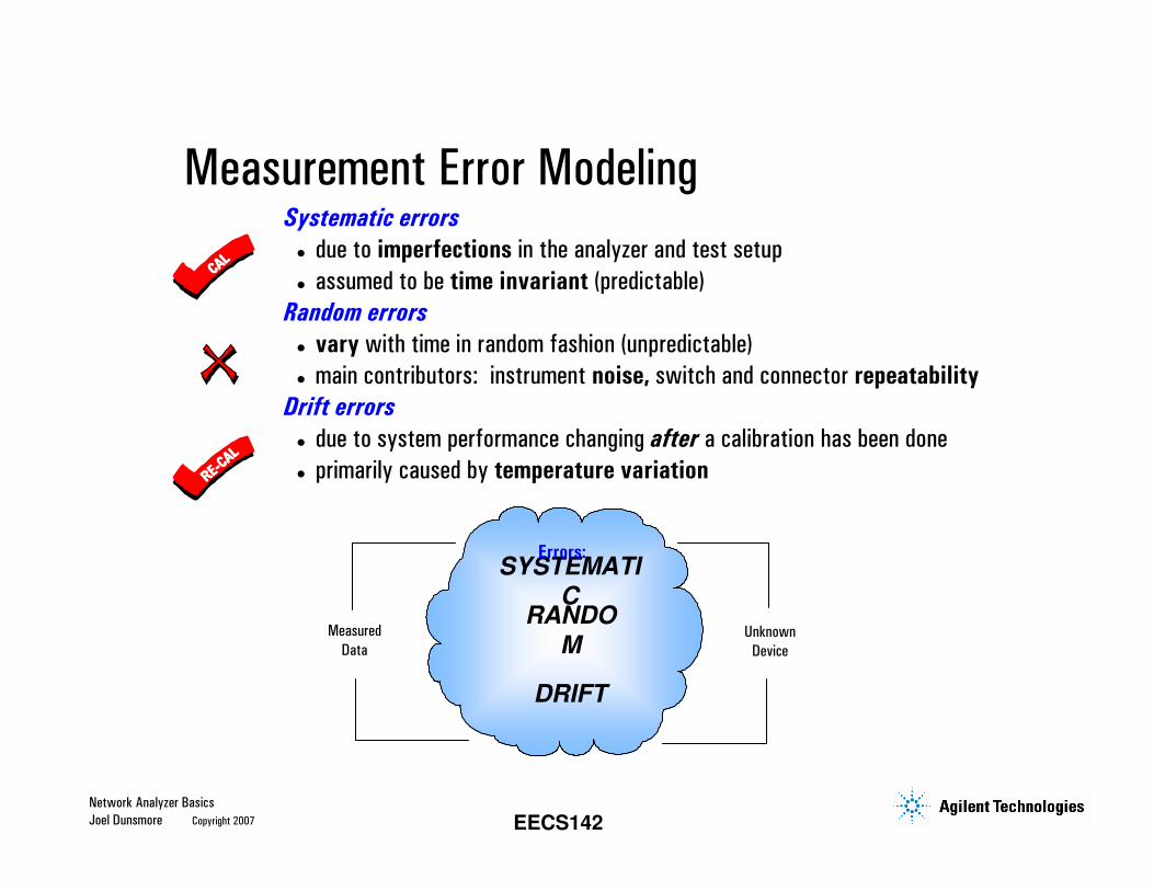
Systematic errors
due to imperfections in the analyzer and test setup
assumed to be time invariant (predictable)
Random errors
vary with time in random fashion (unpredictable)
main contributors: instrument noise, switch and connector repeatability
Drift errors
due to system performance changing after a calibration has been done
primarily caused by temperature variation
Measured
Data
Unknown
Device
SYSTEMATIC
RANDOM
DRIFT
Errors:
CAL
CAL
CAL
CAL
RERERERE----CAL
CAL
CAL
CAL
Measurement Error Modeling
Network Analyzer Basics
Joel Dunsmore Copyright 2007 EECS142
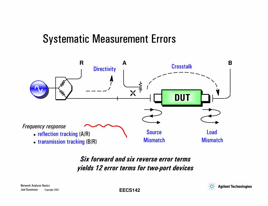
A B
Source
Mismatch
Load
Mismatch
CrosstalkDirectivity
DUT
Frequency response
reflection tracking (A/R)
transmission tracking (B/R)
R
Six forward and six reverse error terms
yields 12 error terms for two-port devices
Systematic Measurement Errors
Network Analyzer Basics
Joel Dunsmore Copyright 2007 EECS142
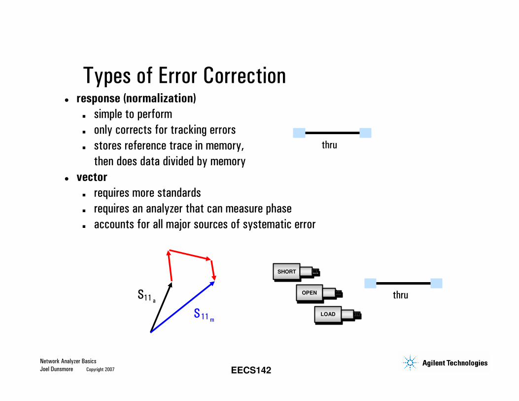
response (normalization)
simple to perform
only corrects for tracking errors
stores reference trace in memory,
then does data divided by memory
vector
requires more standards
requires an analyzer that can measure phase
accounts for all major sources of systematic error
S11 m
S11 a
SHORT
OPEN
LOAD
thru
thru
Types of Error Correction
Network Analyzer Basics
Joel Dunsmore Copyright 2007 EECS142
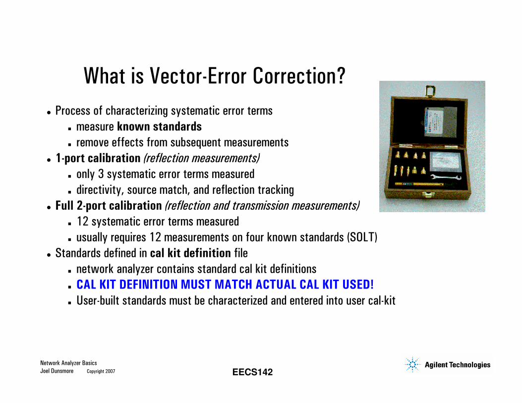
Process of characterizing systematic error terms
measure known standards
remove effects from subsequent measurements
1-port calibration (reflection measurements)
only 3 systematic error terms measured
directivity, source match, and reflection tracking
Full 2-port calibration (reflection and transmission measurements)
12 systematic error terms measured
usually requires 12 measurements on four known standards (SOLT)
Standards defined in cal kit definition file
network analyzer contains standard cal kit definitions
CAL KIT DEFINITION MUST MATCH ACTUAL CAL KIT USED!
User-built standards must be characterized and entered into user cal-kit
What is Vector-Error Correction?
Network Analyzer Basics
Joel Dunsmore Copyright 2007 EECS142
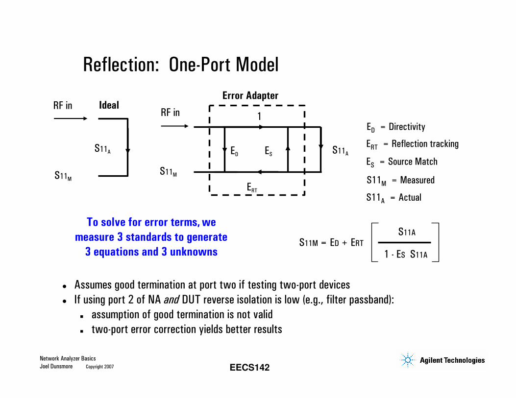
Reflection: One-Port Model
ED = Directivity
ERT = Reflection tracking
ES = Source Match
S11M = Measured
S11A = Actual
To solve for error terms,we
measure 3 standards to generate
3 equations and 3 unknowns
S11M
S11AES
ERT
ED
1RF in
Error Adapter
S11M
S11A
RF in Ideal
Assumes good termination at port two if testing two-port devices
If using port 2 of NA and DUT reverse isolation is low (e.g., filter passband):
assumption of good termination is not valid
two-port error correction yields better results
S11M = ED + ERT
1 - ES S11A
S11A
Network Analyzer Basics
Joel Dunsmore Copyright 2007 EECS142
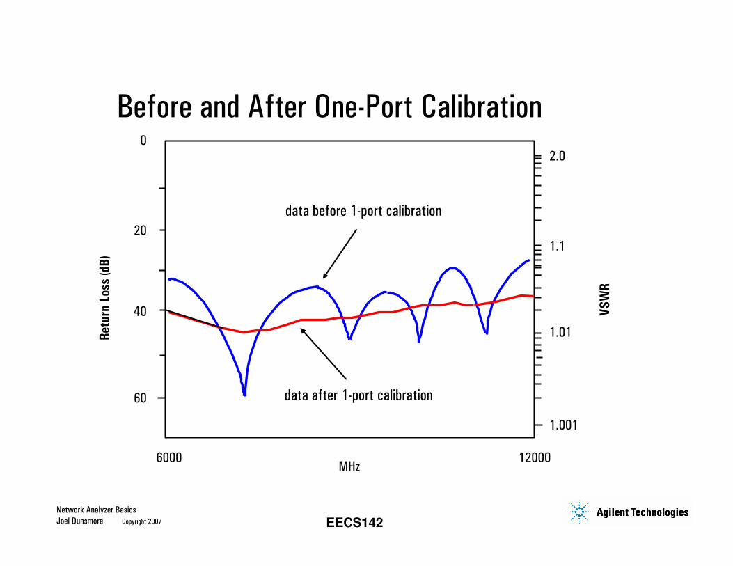
data before 1-port calibration
data after 1-port calibration
0
20
40
60
6000 12000
2.0
Return Loss (d
B)
VSWR
1.1
1.01
1.001
MHz
Before and After One-Port Calibration
Network Analyzer Basics
Joel Dunsmore Copyright 2007 EECS142
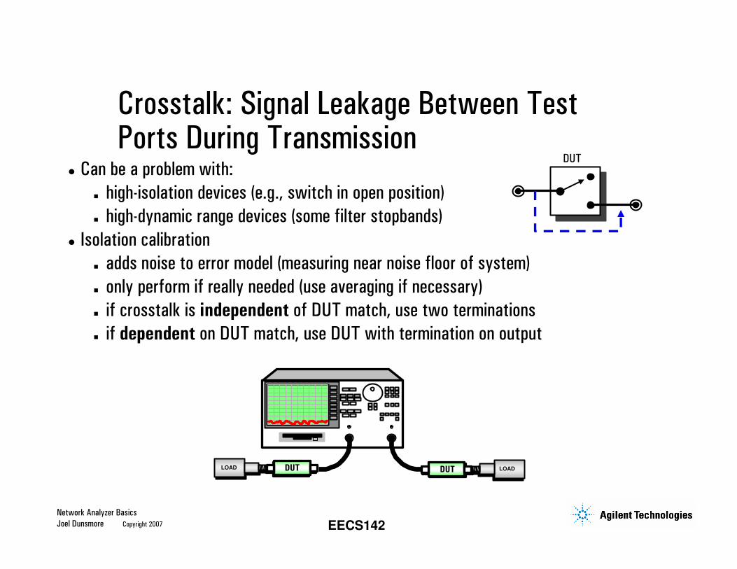
Can be a problem with:
high-isolation devices (e.g., switch in open position)
high-dynamic range devices (some filter stopbands)
Isolation calibration
adds noise to error model (measuring near noise floor of system)
only perform if really needed (use averaging if necessary)
if crosstalk is independent of DUT match, use two terminations
if dependent on DUT match, use DUT with termination on output
DUT
DUT LOADDUTLOAD
Crosstalk: Signal Leakage Between Test Ports During Transmission
Network Analyzer Basics
Joel Dunsmore Copyright 2007 EECS142
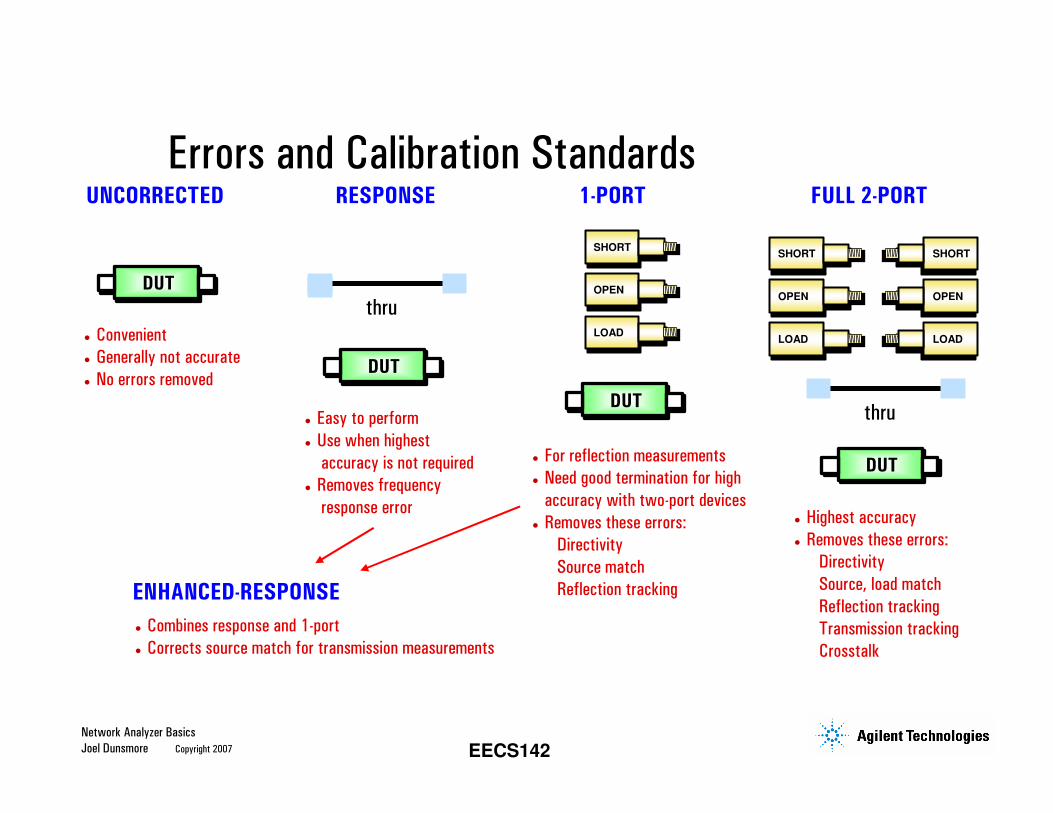
Convenient
Generally not accurate
No errors removed
Easy to perform
Use when highest
accuracy is not required
Removes frequency
response error
For reflection measurements
Need good termination for high
accuracy with two-port devices
Removes these errors:
Directivity
Source match
Reflection tracking
Highest accuracy
Removes these errors:
Directivity
Source, load match
Reflection tracking
Transmission tracking
Crosstalk
UNCORRECTED RESPONSE 1-PORT FULL 2-PORT
DUT
DUT
DUT
DUT
thru
thru
ENHANCED-RESPONSE
Combines response and 1-port
Corrects source match for transmission measurements
SHORT
OPEN
LOAD
SHORT
OPEN
LOAD
SHORT
OPEN
LOAD
Errors and Calibration Standards
Network Analyzer Basics
Joel Dunsmore Copyright 2007 EECS142
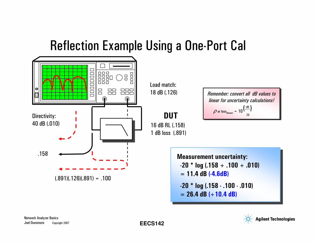
DUT16 dB RL (.158)
1 dB loss (.891)
Load match:
18 dB (.126)
.158
(.891)(.126)(.891) = .100
Directivity:
40 dB (.010)
Measurement uncertainty:
-20 * log (.158 + .100 + .010)
= 11.4 dB (-4.6dB)
-20 * log (.158 - .100 - .010)
= 26.4 dB (+10.4 dB)
Remember: convert all dB values to
linear for uncertainty calculations!
ρ or loss(linear) = 10( )-dB
20
Reflection Example Using a One-Port Cal
Network Analyzer Basics
Joel Dunsmore Copyright 2007 EECS142
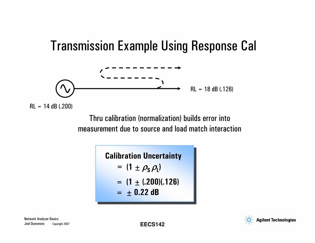
RL = 14 dB (.200)
RL = 18 dB (.126)
Thru calibration (normalization) builds error into
measurement due to source and load match interaction
Calibration Uncertainty
= (1 ± ρρρρS ρρρρL)
= (1 ± (.200)(.126)
= ± 0.22 dB
Transmission Example Using Response Cal
Network Analyzer Basics
Joel Dunsmore Copyright 2007 EECS142
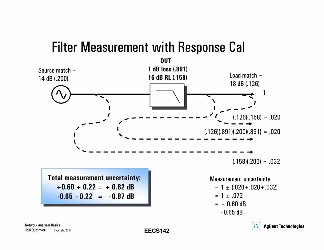
Source match =
14 dB (.200)
1
(.126)(.158) = .020
(.158)(.200) = .032
(.126)(.891)(.200)(.891) = .020
Measurement uncertainty
= 1 ± (.020+.020+.032)
= 1 ± .072
= + 0.60 dB
- 0.65 dB
DUT
1 dB loss (.891)
16 dB RL (.158)
Total measurement uncertainty:
+0.60 + 0.22 = + 0.82 dB
-0.65 - 0.22 = - 0.87 dB
Load match =
18 dB (.126)
Filter Measurement with Response Cal
Network Analyzer Basics
Joel Dunsmore Copyright 2007 EECS142
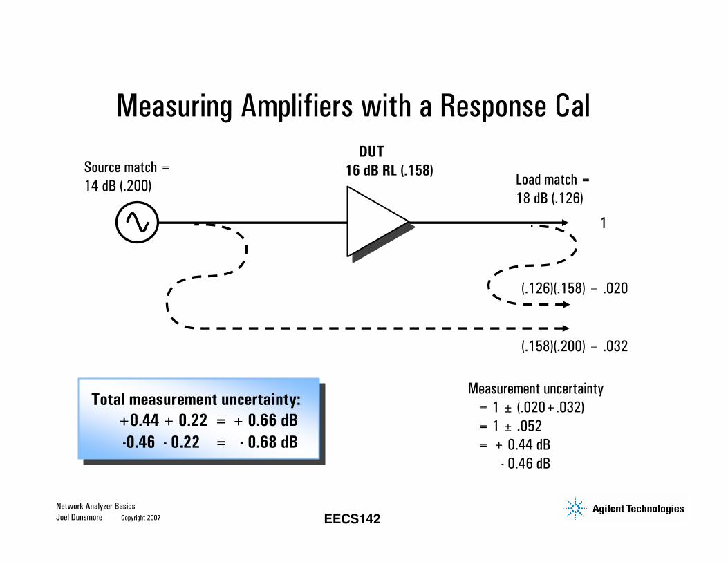
Total measurement uncertainty:
+0.44 + 0.22 = + 0.66 dB
-0.46 - 0.22 = - 0.68 dB
Measurement uncertainty
= 1 ± (.020+.032)
= 1 ± .052
= + 0.44 dB
- 0.46 dB
1
(.126)(.158) = .020
DUT
16 dB RL (.158)
(.158)(.200) = .032
Source match =
14 dB (.200) Load match =
18 dB (.126)
Measuring Amplifiers with a Response Cal
Network Analyzer Basics
Joel Dunsmore Copyright 2007 EECS142
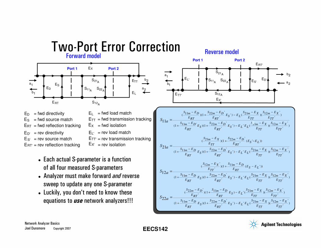
Each actual S-parameter is a function
of all four measured S-parameters
Analyzer must make forward and reverse
sweep to update any one S-parameter
Luckily, you don't need to know these
equations to use network analyzers!!!
Port 1 Port 2E
S11
S21
S12
S22
ESED
ERT
ETT
EL
a1
b1
A
A
A
A
X
a2
b2
Forward model
= fwd directivity
= fwd source match
= fwd reflection tracking
= fwd load match
= fwd transmission tracking
= fwd isolation
ES
ED
ERT
ETT
EL
EX
= rev reflection tracking
= rev transmission tracking
= rev directivity
= rev source match
= rev load match
= rev isolation
ES'
ED'
ERT'
ETT'
EL'
EX'
Port 1 Port 2
S11
S
S12
S22 ES'ED'
ERT'
ETT'
EL'
a1
b1A
A
A
EX'
21A
a2
b2
Reverse modelTwo-Port Error Correction
S a
Sm
ED
ERT
Sm
ED
ERT
ES
EL
Sm
EX
ETT
Sm
EX
ETT
Sm
ED'
ERT
ES
Sm
ED
ERT
ES
EL
EL
Sm
EX
ETT
Sm
EX
ETT
11
111
22 21 12
111
122 21 12
=
−+
−−
− −
+−
+−
−− −
( )('
'' ) ( )(
'
')
( )('
'' ) ' ( )(
'
')
S a
Sm
EX
ETT
Sm
ED
ERT
ES
EL
Sm
ED
ERT
ES
Sm
ED
ERT
ES
EL
21
21 22
111
122
=
−1 +
−−
+−
+−
−
( )('
'( ' ))
( )('
'' ) ' ( )(
'
')E
L
Sm
EX
ETT
Sm
EX
ETT
21 12− −
'S E S E− −(
')( ( ' ))
( )('
'' ) ' ( )(
'
')
m X
ETT
m D
ERT
ES
EL
Sm
ED
ERT
ES
Sm
ED
ERT
ES
EL
EL
Sm
EX
ETT
Sm
EX
ETT
S a
121
11
111
122 21 12
12
+ −
+−
+−
−− −
=
('
')(
(
Sm
ED
ERT
Sm
ED
ERT
S a
22
111
22
−) ' ( )(
'
')
Sm
ED
ERT
ES
EL
Sm
EX
ETT
Sm
EX
ETT
11 21 12−−
− −
+−
=
ES
Sm
ED
ERT
ES
EL
EL
Sm
EX
ETT
Sm
EX
ETT
)('
'' ) ' ( )(
'
')1
22 21 12+
−−
− −
1 +
Network Analyzer Basics
Joel Dunsmore Copyright 2007 EECS142
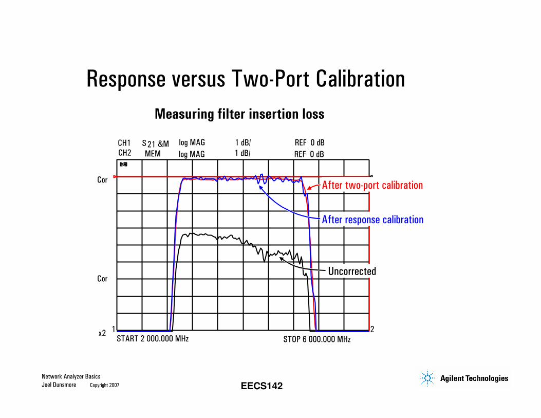
CH1 S 21 &M log MAG 1 dB/ REF 0 dB
Cor
CH2 MEM log MAG REF 0 dB1 dB/
CorUncorrected
After two-port calibration
START 2 000.000 MHz STOP 6 000.000 MHzx2 1 2
After response calibration
Measuring filter insertion loss
Response versus Two-Port Calibration
Network Analyzer Basics
Joel Dunsmore Copyright 2007 EECS142
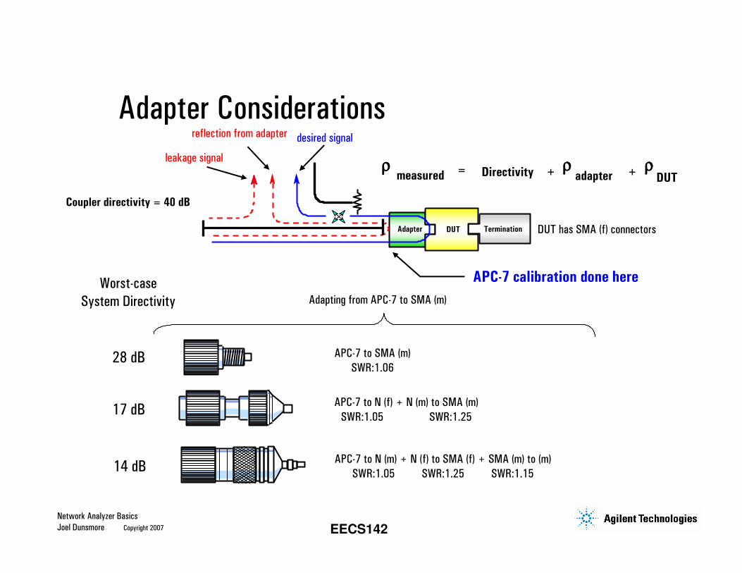
TerminationAdapter DUT
Coupler directivity = 40 dB
leakage signal
desired signalreflection from adapter
APC-7 calibration done here
DUT has SMA (f) connectors
= measured ρρρρ +adapter
ρρρρDUT
ρρρρDirectivity +
Worst-case
System Directivity
28 dB
17 dB
14 dB
APC-7 to SMA (m)
SWR:1.06
APC-7 to N (f) + N (m) to SMA (m)
SWR:1.05 SWR:1.25
APC-7 to N (m) + N (f) to SMA (f) + SMA (m) to (m)
SWR:1.05 SWR:1.25 SWR:1.15
Adapting from APC-7 to SMA (m)
Adapter Considerations
Network Analyzer Basics
Joel Dunsmore Copyright 2007 EECS142
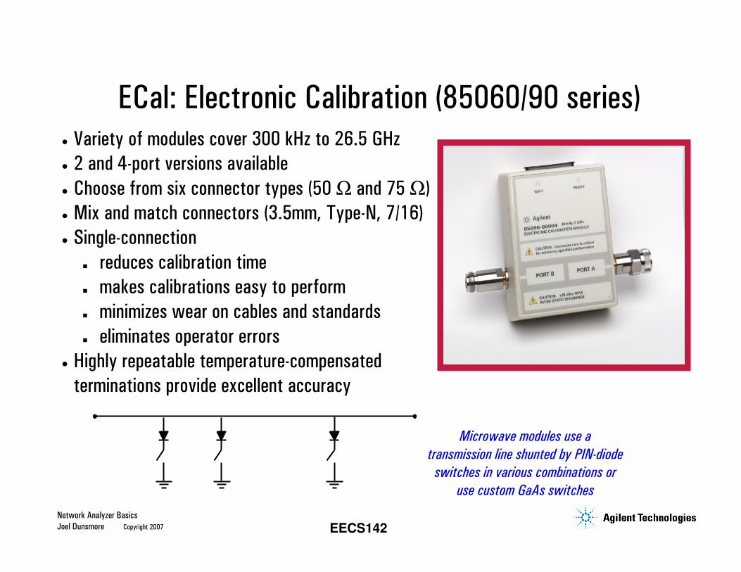
• Variety of modules cover 300 kHz to 26.5 GHz
• 2 and 4-port versions available
• Choose from six connector types (50 Ω and 75 Ω)
• Mix and match connectors (3.5mm, Type-N, 7/16)
• Single-connection
reduces calibration time
makes calibrations easy to perform
minimizes wear on cables and standards
eliminates operator errors
• Highly repeatable temperature-compensated
terminations provide excellent accuracy
85093A Electronic Calibration Module30 kHz - 6 GHz
Microwave modules use a
transmission line shunted by PIN-diode
switches in various combinations or
use custom GaAs switches
ECal: Electronic Calibration (85060/90 series)
Network Analyzer Basics
Joel Dunsmore Copyright 2007 EECS142
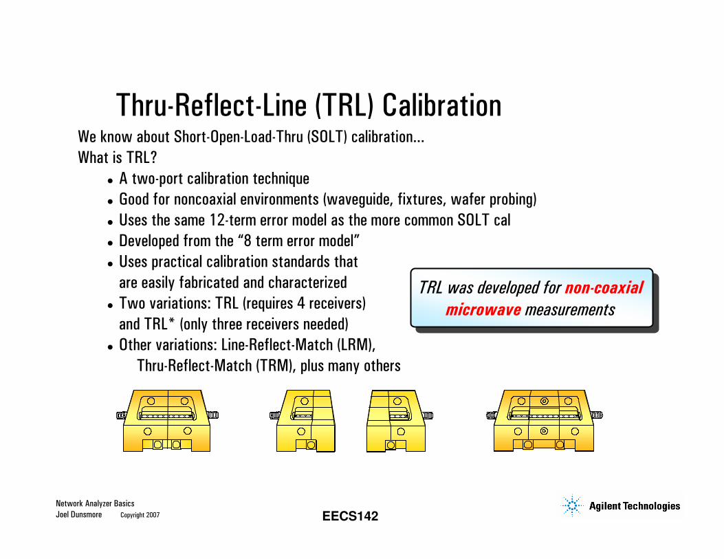
We know about Short-Open-Load-Thru (SOLT) calibration...
What is TRL?
A two-port calibration technique
Good for noncoaxial environments (waveguide, fixtures, wafer probing)
Uses the same 12-term error model as the more common SOLT cal
Developed from the “8 term error model”
Uses practical calibration standards that
are easily fabricated and characterized
Two variations: TRL (requires 4 receivers)
and TRL* (only three receivers needed)
Other variations: Line-Reflect-Match (LRM),
Thru-Reflect-Match (TRM), plus many others
TRL was developed for non-coaxial
microwave measurements
Thru-Reflect-Line (TRL) Calibration
Network Analyzer Basics
Joel Dunsmore Copyright 2007 EECS142
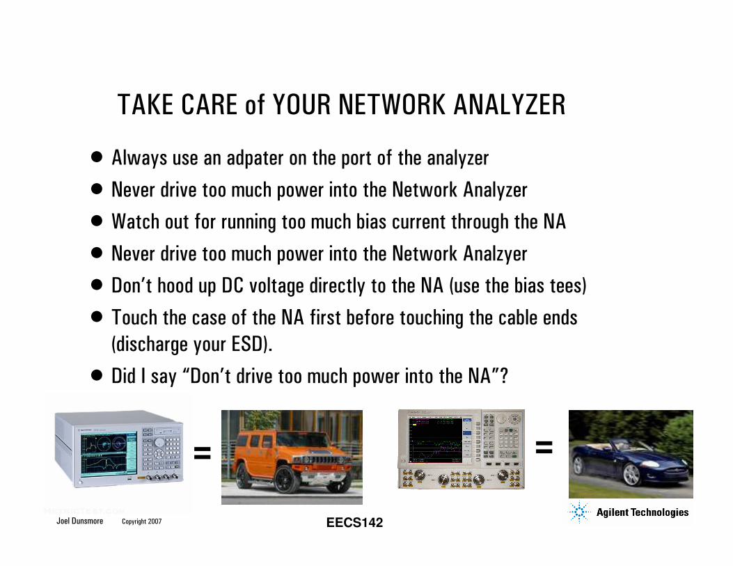
TAKE CARE of YOUR NETWORK ANALYZER
• Always use an adpater on the port of the analyzer
• Never drive too much power into the Network Analyzer
• Watch out for running too much bias current through the NA
• Never drive too much power into the Network Analzyer
• Don’t hood up DC voltage directly to the NA (use the bias tees)
• Touch the case of the NA first before touching the cable ends
(discharge your ESD).
• Did I say “Don’t drive too much power into the NA”?
= =
Network Analyzer Basics
Joel Dunsmore Copyright 2007 EECS142
In Class Demo: Setting up and using the NA
• Start by setting up the start/stop/number of points for your
measurement, under the Stimulus block
• Set the IF BW: 1 KHz for precise measurements, 10 kHz for fast.
• Set the power if you’re measuring an active device, to avoid over
driving the NA
• Select the traces: on the ENA select “display traces” to change
then number of traces shown.
• Hit the Meas key to select what parameter to display
• Hit the MARKER key to put one (or more) markers on the screen
Network Analyzer Basics
Joel Dunsmore Copyright 2007 EECS142
In Class Demo: Setting up and using the NA
• Use the FORMAT to change between Log and Linear
• Use the Scale key to bring up the scale. Use autoscale or select
the scale in dB/div, the reference live value, and reference line
position
• Use the Data->Memory and Data&Mem to save compare traces
(DISPLAY)
• Save your data using “Save S2P”
• Use the equation editor to change the value of your trace
• Use Save/Recall to save your setups


