Network Models Social Media Mining. 2 Measures and Metrics 2 Social Media Mining Network Models Why...

Network Models

Social Media Mining

2Social Media Mining

Measures and Metrics 2Social Media Mining

Network Models

Why should I use network models?

• In may 2011, Facebook had 721 millions users. A Facebook user at the time had an average of 190 users -> a total of 68.5 billion friendships– What are the principal underlying processes

that help initiate these friendships– How can these seemingly independent

friendships form this complex friendship network?

• In social media there are many networks with millions of nodes and billions of edges.– They are complex and it is difficult to analyze

them



Network Models

So, what do we do?

• We design models that generate, on a smaller scale, graphs similar to real-world networks.

• Hoping that these models simulate properties observed in real-world networks well, the analysis of real-world networks boils down to a cost-efficient measuring of different properties of simulated networks– Allow for a better understanding of phenomena

observed in real-world networks by providing concrete mathematical explanations; and

– Allow for controlled experiments on synthetic networks when real-world networks are not available.

• These models are designed to accurately model properties observed in real-world networks



Network Models

Power-law Distribution, High Clustering Coefficient, Small Average Path Length

Properties of Real-World Networks



Network Models

Degree Distribution



Network Models

Degree Distribution

• Consider the distribution of wealth among individuals. Most individuals have average capitals, whereas a few are considered wealthy. In fact, we observe exponentially more individuals with average capital than the wealthier ones.

• Similarly, consider the population of cities. Often, a few metropolitan areas are densely populated, whereas other cities have an average population size.

• In social media, we observe the same phenomenon regularly when measuring popularity or interestingness for entities.



Network Models

Degree Distribution

• Many sites are visited less than a 1,000 times a month whereas a few are visited more than a million times daily.

• Social media users are often active on a few sites whereas some individuals are active on hundreds of sites.

• There are exponentially more modestly priced products for sale compared to expensive ones.

• There exist many individuals with a few friends and a handful of users with thousands of friends

(Degree Distribution)



Network Models

Power Law Distribution

• When the frequency of an event changes as a power of an attribute -> the frequency follows a power-law

• Let p(k) denote the fraction of individuals having degree k.

b: the power-law exponent and its value is typically in the range of [2, 3]a: power-law intercept



Network Models

Power Law Distribution

A typical shape of a power-law distribution• Many real-world networks

exhibit a power-law distribution.

• Power laws seem to dominate in cases where the quantity being measured can be viewed as a type of popularity.

• A power-law distribution implies that small occurrences are common, whereas large instances are extremely rare

Log-Log plot



Network Models

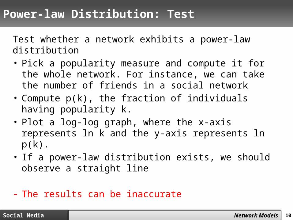
Power-law Distribution: Test

Test whether a network exhibits a power-law distribution• Pick a popularity measure and compute it for the

whole network. For instance, we can take the number of friends in a social network

• Compute p(k), the fraction of individuals having popularity k.

• Plot a log-log graph, where the x-axis represents ln k and the y-axis represents ln p(k).

• If a power-law distribution exists, we should observe a straight line

- The results can be inaccurate



Network Models

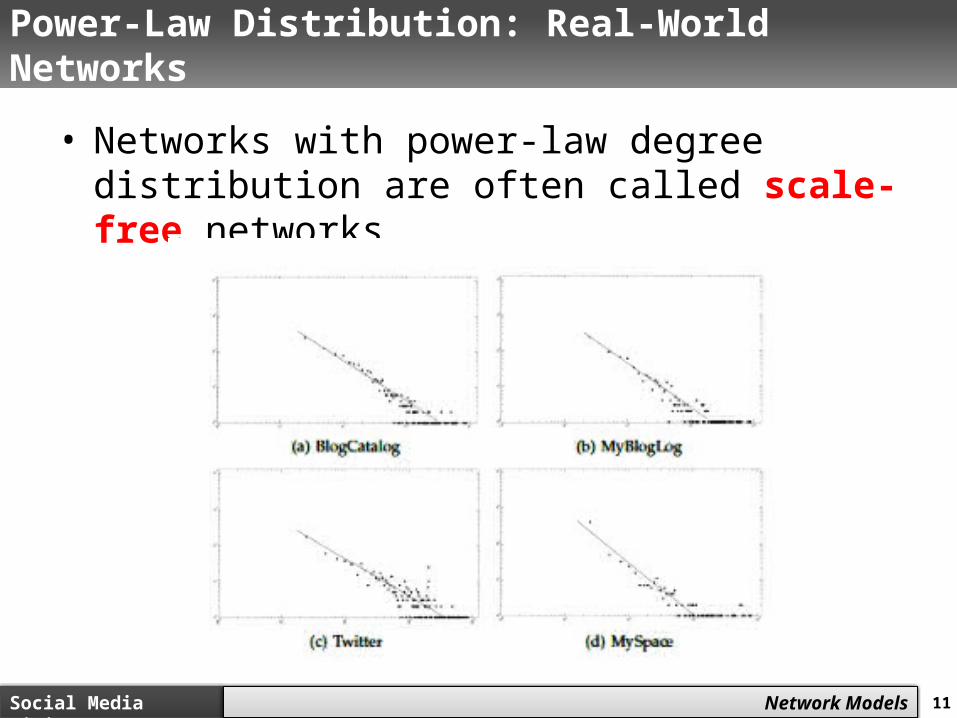
Power-Law Distribution: Real-World Networks

• Networks with power-law degree distribution are often called scale-free networks



Network Models

Clustering Coefficient



Network Models

Clustering Coefficient

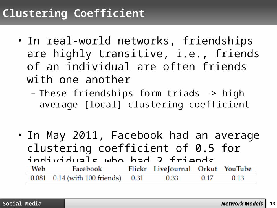
• In real-world networks, friendships are highly transitive, i.e., friends of an individual are often friends with one another– These friendships form triads -> high average

[local] clustering coefficient

• In May 2011, Facebook had an average clustering coefficient of 0.5 for individuals who had 2 friends.



Network Models

Average Path Length



Network Models

The Average Shortest Path

• In real-world networks, any two members of the network are usually connected via short paths. In other words, the average path length is small– Six degrees of separation:

• Stanley Milgram In the well-known small-world experiment conducted in the 1960’s conjectured that people around the world are connected to one another via a path of at most 6 individuals

– Four degrees of separation:• Lars Backstrom et al. in May 2011, the average

path length between individuals in the Facebook graph was 4.7. (4.3 for individuals in the US)



Network Models

Stanley Milgram’s Experiments

• Random people from Nebraska were asked to send a letter (via intermediaries) to a stock broker in Boston

• S/he could only send to someone with whom they were on a first-name basis

Among the letters that reached the target, the average path length was six.

Stanley Milgram (1933-1984)



Network Models

Random Graphs



Network Models

Random Graphs

• We start with the most basic assumption on how friendships are formed.

Random Graph’s main assumption:

Edges (i.e., friendships) between nodes (i.e., individuals) are formed randomly.



Network Models

Random Graph Model – G(n,p)

• We discuss two random graph models• Formally, we can assume that for a graph

with a fixed number of nodes n, any of the edges can be formed independently, with probability p. This graph is called a random graph and we denote it as G(n, p) model.– This model was first proposed independently

by Edgar Gilbert and Solomonoff and Rapoport.

C(n, 2) or is # of combinations of two objects from a set of n objects



Network Models

Random Graph Model - G(n,m)

• Another way of randomly generating graphs is to assume both number of nodes n and number of edges m are fixed. However, we need to determine which m edges are selected from the set of possible edges– Let denote the set of graphs with n nodes and m

edges– There are |Ω| different graphs with n nodes and m edges

• To generate a random graph, we uniformly select one of the |Ω| graphs (the selection probability is 1/|Ω|)This model proposed first by Paul Erdos and Alfred Renyi



Network Models

Modeling Random Graphs, Cont.

• In the limit (when n is large), both models (G(n, p) and G(n, m)) act similarly– The expected number of edges in G(n, p) is– We can set and in the limit, we

should get similar results.

Differences:– The G(n, m) model contains a fixed number of

edges– The G(n, p) model is likely to contain none or

all possible edges



Network Models

Expected Degree

The expected number of edges connected to a node (expected degree) in G(n, p) is c=(n - 1)p• Proof:– A node can be connected to at most n-1 nodes

(or n-1 edges)– All edges are selected independently with

probability p– Therefore, on average, (n - 1)p edges are

selected

• C=(n-1)p or equivalently,



Network Models

Expected Number of Edges

• The expected number of edges in G(n, p) is p

• Proof:– Since edges are selected independently, and

we have a maximum edges, the expected number of edges is p



Network Models

The probability of Observing m edges

Given the G(n, p) process, the probability of observing m edges is binomial distribution

• Proof:– m edges are selected from the possible

edges. – These m edges are formed with probability pm

and other edges are not formed (to guarantee the existence of only m edges) with probability



Network Models

• For a demo:• http://

www.cs.purdue.edu/homes/dgleich/demos/erdos_renyi/er-150.gif

• Create your own demo:• http://www.cs.purdue.edu/homes/dgleich/demos/e

rdos_renyi/

Evolution of Random Graphs

http://www.cs.purdue.edu/homes/dgleich/demos/erdos_renyi/er-150.gif



http://www.cs.purdue.edu/homes/dgleich/demos/erdos_renyi/

http://www.cs.purdue.edu/homes/dgleich/demos/erdos_renyi/



Network Models

The Giant Component

• In random graphs, when nodes form connections, after some time, a large fraction of nodes get connected, i.e., there is a path between any pair of them.

• This large fraction forms a connected component, commonly called the largest connected component or the giant component.

• In random graphs:– p = 0 the size of the giant component is 0– p = 1 the size of the giant component is n



Network Models

The Giant Component

Probability (p)

0.0 0.055 0.11 1.0

Average node degree (c)

0.0 0.8 ~1 n-1 = 9

Diameter 0 2 6 1Giant component size

0 4 7 10

Average path length

0.0 1.5 2.66 1.0



Network Models

Phase Transition

• The point where diameter value starts to shrink in a random graph is called the Phase Transition.

• In a random graph, phase transition happens when average node degree, c = 1, or when p = 1/(n-1)

• At the point of Phase Transition, the following phenomena are observed:– The giant component that just started to

appear, starts grow, and– The diameter that just reached its maximum

value, starts decreasing.



Network Models

Why c=1?

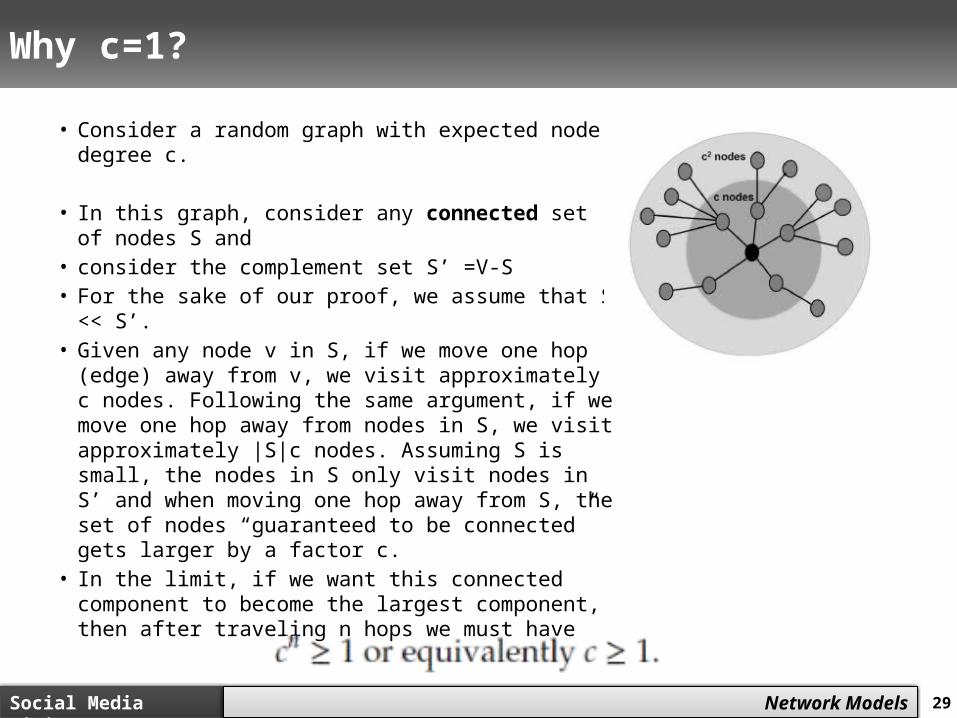
• Consider a random graph with expected node degree c.

• In this graph, consider any connected set of nodes S and

• consider the complement set S’ =V-S• For the sake of our proof, we assume that S

<< S’. • Given any node v in S, if we move one hop

(edge) away from v, we visit approximately c nodes. Following the same argument, if we move one hop away from nodes in S, we visit approximately |S|c nodes. Assuming S is small, the nodes in S only visit nodes in S’ and when moving one hop away from S, the set of nodes “guaranteed to be connected” gets larger by a factor c.

• In the limit, if we want this connected component to become the largest component, then after traveling n hops we must have



Network Models

Properties of Random Graphs



Network Models

Degree Distribution

• When computing degree distribution, we estimate the probability of observing P(dv = d) for node v

• For a random graph generated by G(n,p) this probability is

• This is a binomial degree distribution. In the limit this will become the Poisson degree distribution



Network Models

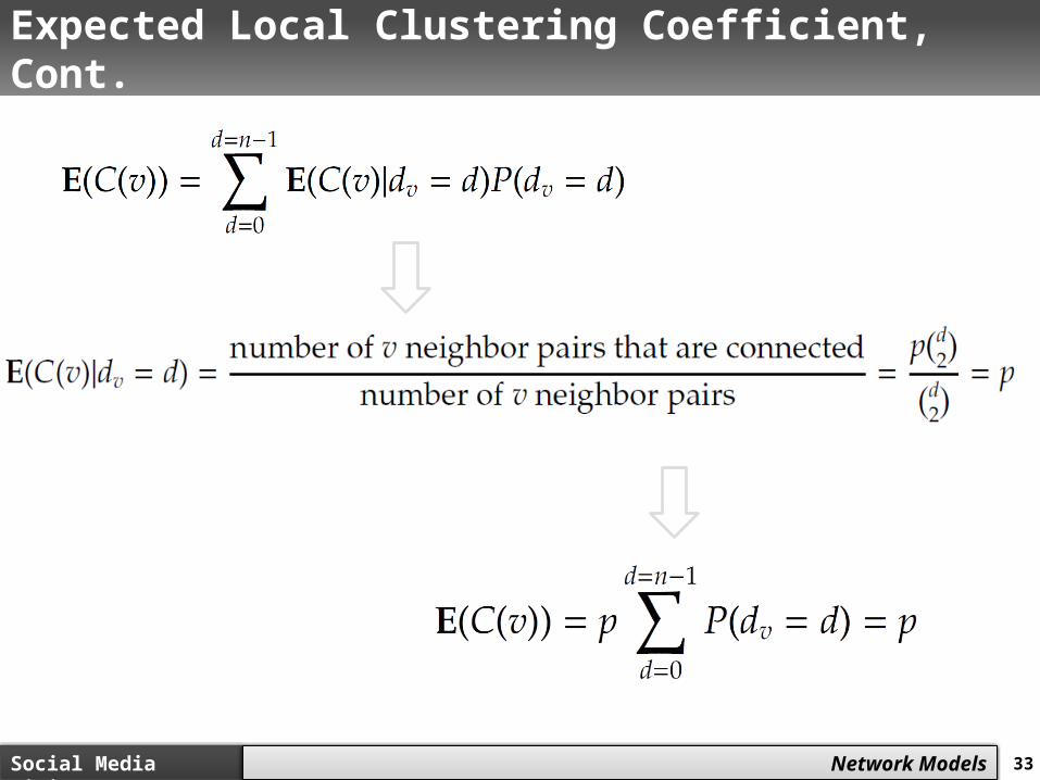
Expected Local Clustering Coefficient

The expected local clustering coefficient for node v of a random graph generated by G(n, p) is p• Proof:

– v can have different degrees depending on the random procedure so the expected value is,



Network Models

Expected Local Clustering Coefficient, Cont.



Network Models

Global Clustering Coefficient

The global clustering coefficient of a random graph generated by G(n, p) is p• Proof:– The global clustering coefficient of any graph

defines the probability of two neighbors of the same node that are connected.

– In a random graph, for any two nodes, this probability is the same and is equal to the generation probability p that determines the probability of two nodes getting connected



Network Models

The Average Path Length

The average path length in a random graph is



Network Models

Modeling Real-World Networks with Random Graphs

• Compute the average degree c, then compute p, by using: c/(n-1)= p, then generate the random graph

• How good is the model?– random graphs perform well in modeling the

average path lengths; however, when considering the transitivity, the random graph model drastically underestimates the clustering coefficient.



Network Models

Real-World Networks and Simulated Random Graphs



Network Models

Small-World Model



Network Models

Small-world Model

• Small-world Model also known as the Watts and Strogatz model is a special type of random graphs with small-world properties, including:– Short average path length and;– High clustering.

• It was proposed by Duncan J. Watts and Steven Strogatz in their joint 1998 Nature paper



Network Models

Small-world Model

• In real-world interactions, many individuals have a limited and often at least, a fixed number of connections

• In graph theory terms, this assumption is equivalent to embedding individuals in a regular network.

• A regular (ring) lattice is a special case of regular networks where there exists a certain pattern on how ordered nodes are connected to one another.

• In particular, in a regular lattice of degree c, nodes are connected to their previous c/2 and following c/2 neighbors. Formally, for node set , an edge exists between node i and j if and only if



Network Models

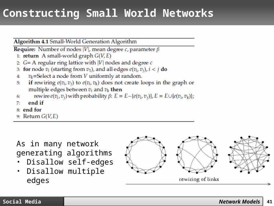
Constructing Small World Networks

As in many network generating algorithms• Disallow self-edges• Disallow multiple

edges



Network Models

Small-World ModelProperties



Network Models

Degree Distribution

• The degree distribution for the small-world model is

• In practice, in the graph generated by the small world model, most nodes have similar degrees due to the underlying lattice.



Network Models

Regular Lattice and Random Graph: Clustering Coefficient and Average Path Length• Regular Lattice:• Clustering Coefficient (high):

• Average Path Length (high): n/2c• Random Graph:• Clustering Coefficient (low): p• Average Path Length (ok!) : ln |V|/

ln c



Network Models

What happens in Between?

• Does smaller average path length mean smaller clustering coefficient?

• Does larger average path length mean larger clustering coefficient?

• Through numerical simulation• As we increase p from 0 to 1• Fast decrease of average

distance• Slow decrease in clustering

coefficient



Network Models

Change in Clustering Coefficient and Average Path Length as a Function of the Proportion of Rewired Edges

10% of links rewired1% of links rewired

No exact analytical solution

Exact analytical solution



Network Models

Clustering Coefficient for Small-world model with rewiring

• The probability that a connected triple stays connected after rewiring consists of two parts 1. The probability that none of the 3

edges were rewired is (1-p)3

2. The probability that other edges were rewired back to form a connected triple is very small and can be ignored

• Clustering coefficient

p



Network Models

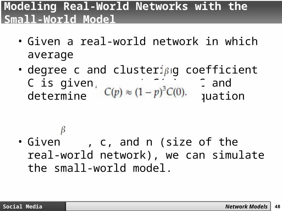
Modeling Real-World Networks with the Small-World Model

• Given a real-world network in which average

• degree c and clustering coefficient C is given, we set C(p) = C and determine (=p) using equation

• Given , c, and n (size of the real-world network), we can simulate the small-world model.



Network Models

Real-World Network and Simulated Graphs



Network Models

Preferential Attachment Model



Network Models

Preferential Attachment: An Example

• Networks:– When a new user joins the network, the

probability of connecting to existing nodes is proportional to the nodes’ degree

• Distribution of wealth in the society:– The rich get richer



Network Models

Constructing Scale-free Networks

• Graph G(V0, E) is given

• For any new node v to the graph– Connect v to a random node vi V0, with

probability



Network Models

Properties of the Preferential Attachment

Model



Network Models

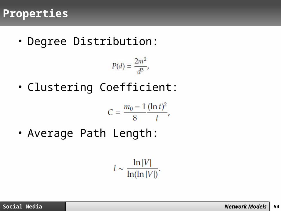
Properties

• Degree Distribution:

• Clustering Coefficient:

• Average Path Length:



Network Models

Modeling Real-World Networks with the Preferential Attachment Model

• Similar to random graphs, we can simulate real-world networks by generating a preferential attachment model by setting the expected degree m (see Algorithm 4.2 – Slide 52)



Network Models

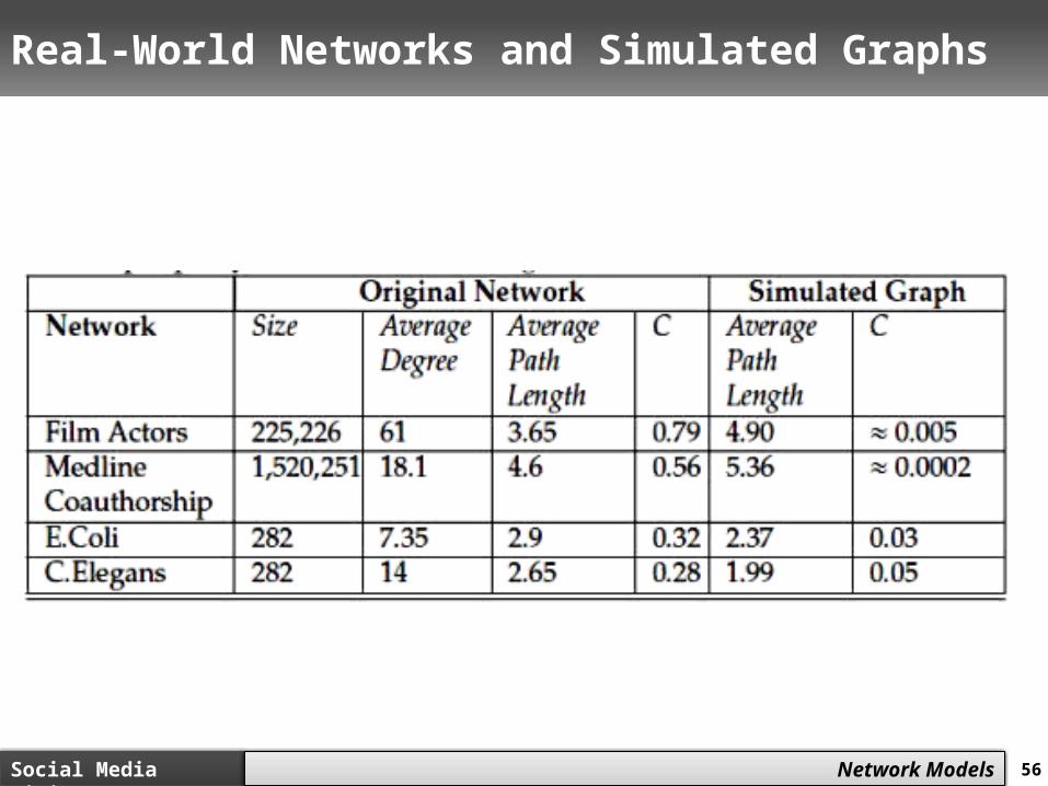
Real-World Networks and Simulated Graphs

Date post:	18-Dec-2015
Category:	Documents
Upload:	owen-dean
View:	218 times
Download:	0 times

Network Models Social Media Mining. 2 Measures and Metrics 2 Social Media Mining Network Models Why...

Documents