109
Prof. Dr.-Ing. I. Willms Network Theory 1 S. 1 Fachgebiet Nachrichtentechnische Systeme NTS Network Theory 1 Analoge Netzwerke Prof. Dr.-Ing. Ingolf Willms and Prof. Dr.-Ing. Peter Laws
Prof. Dr.-Ing. I. Willms Network Theory 1 S. 1
FachgebietNachrichtentechnische Systeme
N T S
Network Theory 1Analoge Netzwerke
Prof. Dr.-Ing. Ingolf Willms and
Prof. Dr.-Ing. Peter Laws

Prof. Dr.-Ing. I. Willms Network Theory 1 S. 2
FachgebietNachrichtentechnische Systeme
N T S
Chapter 1
Introduction and Basics

Prof. Dr.-Ing. I. Willms Network Theory 1 S. 3
FachgebietNachrichtentechnische Systeme
N T S
1.1 Preliminary remarks
Components like resistor, coil etc. are network elements
Two-poles have 2 pins accessible
Two-ports have 4 pins
• Network analysis: gives mathematical description of network properties
• Network synthesis: gives structure and values of components due to given task
Two main tasks of network theory:
Prof. Dr.-Ing. I. Willms Network Theory 1 S. 4
FachgebietNachrichtentechnische Systeme
N T S
1.1 Preliminary remarks
Three solutions steps of network synthesis:
1. Solution step 1: Network characterization by a given characterizing Network function (specification)
2. Solution step 2: Approximation of characterizing Network function by a realizable Network function
3. Solution step 3: Realization of the found realizable network function by a selected circuit (design)

Prof. Dr.-Ing. I. Willms Network Theory 1 S. 5
FachgebietNachrichtentechnische Systeme
N T S
1.1 Preliminary remarks
Solution step 1:
Characterizing network functions can be:
• Impedance function of a LTI two-pole network (one portnetwork)
• A transfer function of a LTI two-port network (or its systemfunction)
• The phase angle or a phase delay or the magnitude of the transfer function
( )cZ j
( )cH
( ) ( )g

Prof. Dr.-Ing. I. Willms Network Theory 1 S. 6
FachgebietNachrichtentechnische Systeme
N T S
1.1 Preliminary remarks
Frequency domain
A tolerance scheme for of a low-pass( )aH
Example of a characterizing network function and its approximation

Prof. Dr.-Ing. I. Willms Network Theory 1 S. 7
FachgebietNachrichtentechnische Systeme
N T S
1.1 Preliminary remarks
Time domain
Characterizing impulse response (Tolerance pattern for an impulse response)

Prof. Dr.-Ing. I. Willms Network Theory 1 S. 8
FachgebietNachrichtentechnische Systeme
N T S
1.1 Preliminary remarks
Realization by:
• finite number of linear elements
• time invariant elements (LTI elements)
• passive elements
Additional possibilities:• active LTI elements
• controlled voltage + current sourcesDanger:
• Poles in right p-plane
• Instability (2 cases) In best case useful only for signal generators
Solution step 2:

Prof. Dr.-Ing. I. Willms Network Theory 1 S. 9
FachgebietNachrichtentechnische Systeme
N T S
1.1 Preliminary remarksTo observe:
Rational real fractional network function cannot realize in general
a) Arbitrary phase function
b) Arbitrary magnitude
c) Thus also no abitrary
( ) ( )c CH
( )cH
Thus differences are always to be expected between desiredfunctions (index c) and realisable functions (index a).
Differences are measured by in a certain range 1 2
will depend on parameters of
( )ch t
( )eH j( )eH j ( )aH j
( ) ( ) ( )e a cH j H H

Prof. Dr.-Ing. I. Willms Network Theory 1 S. 10
FachgebietNachrichtentechnische Systeme
N T S
1.1 Preliminary remarks( )eh tThe typical error function in time domain:
( ) ( ) ( )e a ch t h t h t with approximations intervall 1 2t t t
Approximation criteria:1. CHEBYSHEF criterion or regular approximation:
Limits max. deviation, example see S.6 2. Criterion of the smallest mean square error:
2
1
2min ( )eH d
or2
1
2min ( )t
et
h t dtSolution of the approximation tasks:
- Simple if approx. function linearly depends on approx. parameters
- Leads to solution of linear system of equations and can be extended byweighting functions
2
1
2min ( ) ( )eH Q d
2
1
2min ( ) ( )t
et
h t q t dtor
Prof. Dr.-Ing. I. Willms Network Theory 1 S. 11
FachgebietNachrichtentechnische Systeme
N T S
1.1 Preliminary remarksApproximation criteria:
3. Criterion of maximum smoothing: The error function and its derivatives should show for orders as high as possible the value of zero at a prescribed location within the approximation interval.
4. Interpolation criterion: Adjusting the approximation parameters in such a way that the error function at given discrete points within the approximation interval is zero.
The number of these discrete interpolation points corresponds to the number of approximation parameters.
Disadvantage: Large deviations at many other locations!

Prof. Dr.-Ing. I. Willms Network Theory 1 S. 12
FachgebietNachrichtentechnische Systeme
N T S
1.1 Preliminary remarksSolution step 3: Circuit realization
- Several realization possibilities exist depending on certain defaults:
• a passive or active network
• a pure reactance network
• an active or passive RC network
• a network with passive symmetrical bridges
• arrangements of pieces of line (for MW frequencies)
- Networks composed with a minimum of components should also be preferred

Prof. Dr.-Ing. I. Willms Network Theory 1 S. 13
FachgebietNachrichtentechnische Systeme
N T S
Chapter 1
Introduction
1.2 LTI Concentrated Network Elements
Prof. Dr.-Ing. I. Willms Network Theory 1 S. 14
FachgebietNachrichtentechnische Systeme
N T S
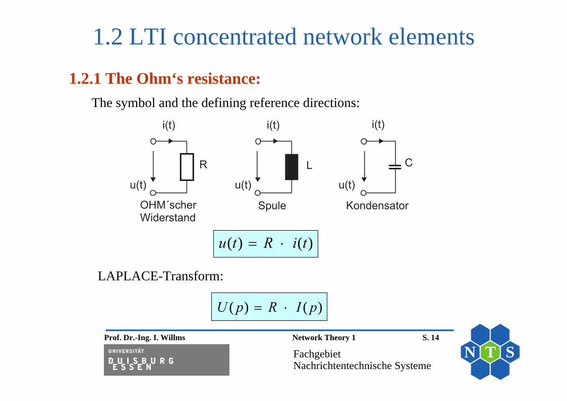
1.2 LTI concentrated network elements1.2.1 The Ohm‘s resistance:
! " #
$
The symbol and the defining reference directions:
( ) ( )u t R i t
LAPLACE-Transform:
( ) ( )U p R I p

Prof. Dr.-Ing. I. Willms Network Theory 1 S. 15
FachgebietNachrichtentechnische Systeme
N T S
1.2 LTI concentrated network elements1.2.2 The capacity C
( )( ) du ti t Cdt
0
01( ) ( ) ( )
t
t
u t u t i dC
The relationship between the current i(t) and voltage u(t) of an electric capacitor is described as:
as well as
Laplace transform:
( ) ( )I p p C U p Admittance: ( )Y p p C
Impedance: Z(p) = 1 / Y(p)

Prof. Dr.-Ing. I. Willms Network Theory 1 S. 16
FachgebietNachrichtentechnische Systeme
N T S
1.2 LTI concentrated network elements1.2.3 The inductivity L
( )( ) di tu t Ldt
and0
01( ) ( ) ( )
t
t
i t i t u dL
Laplace transform:
( ) ( )U p pL I p

Prof. Dr.-Ing. I. Willms Network Theory 1 S. 17
FachgebietNachrichtentechnische Systeme
N T S
1.2 LTI concentrated network elements
1L
1.2.4 The ideal transformer:The transmission characteristics of a lossless transformer with leakage fieldin the time domain:
1 21 1
1 22 2
( )
( )
di diu t L Mdt dtdi diu t M Ldt dt
with: primary inductivity
2L : secondary inductivity
Laplace transform with zero initial condition gives:
1 1 1 2
2 1 2 2
( ) ( ) ( )( ) ( ) ( )
U p pL I p pM I pU p pM I p pL I p

Prof. Dr.-Ing. I. Willms Network Theory 1 S. 18
FachgebietNachrichtentechnische Systeme
N T S
1.2 LTI concentrated network elements
The relation between the ideal transformer and its transmission characteristics:
1 2
1 2
( ) ( )1( ) ( )
u t ü u t
i t i tü
in Laplace transforms:
1 2
1 2
( ) ( )1( ) ( )
U p ü U p
I p I pü
where ü is transformer constant
1 1
2 2
w Lüw L

Prof. Dr.-Ing. I. Willms Network Theory 1 S. 19
FachgebietNachrichtentechnische Systeme
N T S
1.2 LTI concentrated network elements1.2.5 The ideal Gyrator Changes resistance into conductance and vice versa or capacitors to coils
• Voltage-current relationship of ideal gyrators:
1 2( ) ( )i t g u t
2 1( ) ( )i t g u t Laplace transform 1 2( ) ( )I p g U p
2 1( ) ( )I p g U p
(g is gyrator´s value)

Prof. Dr.-Ing. I. Willms Network Theory 1 S. 20
FachgebietNachrichtentechnische Systeme
N T S
1.2 LTI concentrated network elements
1 2( ) ( )I p g U p
%
Symbol of an ideal gyrator with the reference directions
2
1 1( )( )e
a
Z pg Z p
with
1
1
( )( )( )e
U pZ pI p
the input impedance
2
2
( )( )( )a
U pZ pI p
the load impedance
2 1( ) ( )I p g U p 1 2 2
21 2 2
( ) ( ) /( ) ( )( ) ( ) ( )
U p I p g I pI p gU p g U p

Prof. Dr.-Ing. I. Willms Network Theory 1 S. 21
FachgebietNachrichtentechnische Systeme
N T S
1.2 LTI concentrated network elements1Examples A and B with 1 1 1g
g
g mS C F R R kR
32 6 2
1 1 1A: ( ) ( ) 10( ) 10 1a e
a
Z p R Z pg Z p S k
2
6
6 2 6 6 2
1 1B: ( ) 1/ ( )( )
1 10 = 110 1/( 10 ) 10
a ea
Z p pC Z pg Z p
p F p HS p F S

Prof. Dr.-Ing. I. Willms Network Theory 1 S. 22
FachgebietNachrichtentechnische Systeme
N T S
1.2 LTI concentrated network elements1.2.6 Independent sources:
There are two different kinds of independent sources:
1. The independent (ideal) voltage supply:
qu (t)qU (p)
u(t) U(p)
2. The independent (ideal) current supply:
(t)iq (p)Iq
i(t) I(p)independent of
independent of

Prof. Dr.-Ing. I. Willms Network Theory 1 S. 23
FachgebietNachrichtentechnische Systeme
N T S
1.2 LTI concentrated network elements
&
'
' '
(
' (
)
' (
(
*
Symbols of uncontrolled sources and reference directions
1) Independent (ideal) voltage supply
2) Voltage supply with an internal resistance
3) Independent (ideal) current source
4) Current source with an internal resistance

Prof. Dr.-Ing. I. Willms Network Theory 1 S. 24
FachgebietNachrichtentechnische Systeme
N T S
1.2 LTI concentrated network elements1.2.7 Dependent sources:
Symbols of dependent sources (controlled) and reference directions of the electricity
' + '
' ' +
+
' '
'
+ +
'
'
*
, ' + ' , ' +
Voltage-controlled voltage supply Current-controlled voltage supply
Voltage-controlled current source Current-controlled current source
Prof. Dr.-Ing. I. Willms Network Theory 1 S. 25
FachgebietNachrichtentechnische Systeme
N T S
1.2 LTI concentrated network elements
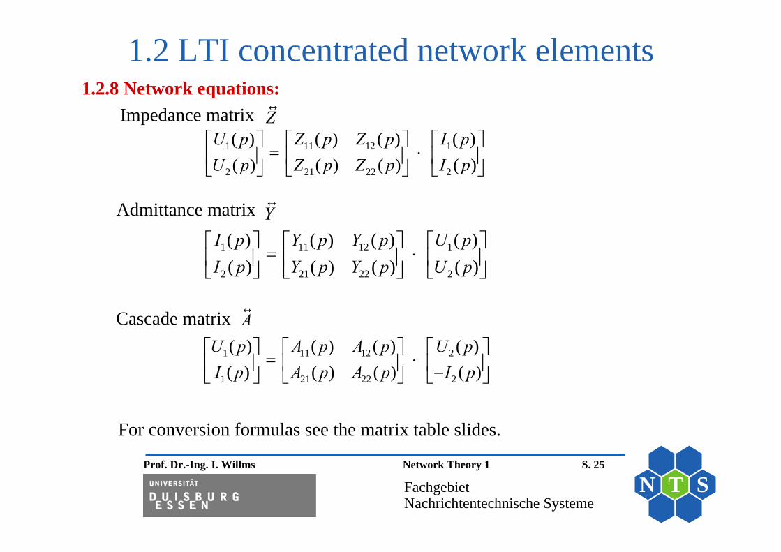
1 11 12 1
2 21 22 2
( ) ( ) ( ) ( )( ) ( ) ( ) ( )
U p Z p Z p I pU p Z p Z p I p
Impedance matrix Z
Admittance matrix Y
1 11 12 1
2 21 22 2
( ) ( ) ( ) ( )( ) ( ) ( ) ( )
I p Y p Y p U pI p Y p Y p U p
Cascade matrix A
1 11 12 2
1 21 22 2
( ) ( ) ( ) ( )( ) ( ) ( ) ( )
U p A p A p U pI p A p A p I p
For conversion formulas see the matrix table slides.
1.2.8 Network equations:

Prof. Dr.-Ing. I. Willms Network Theory 1 S. 26
FachgebietNachrichtentechnische Systeme
N T S
Chapter 1
Introduction
1.3 Network Topology
Prof. Dr.-Ing. I. Willms Network Theory 1 S. 27
FachgebietNachrichtentechnische Systeme
N T S
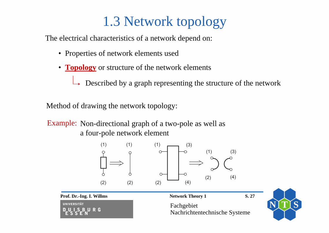
1.3 Network topologyThe electrical characteristics of a network depend on:
• Properties of network elements used
• Topology or structure of the network elements
Described by a graph representing the structure of the network
*
*
Non-directional graph of a two-pole as well as a four-pole network element
Example:
Method of drawing the network topology:

Prof. Dr.-Ing. I. Willms Network Theory 1 S. 28
FachgebietNachrichtentechnische Systeme
N T S
1.3 Network topology
-
*
. . /
-
*. 0
'
'
' 0' . /
' .
' -
' *
'
*
. / 0 .
-
A given network and the nondirectional graph following from it
Prof. Dr.-Ing. I. Willms Network Theory 1 S. 29
FachgebietNachrichtentechnische Systeme
N T S
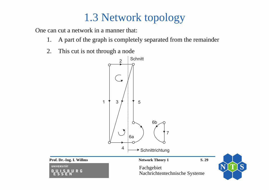
1.3 Network topologyOne can cut a network in a manner that:
1. A part of the graph is completely separated from the remainder
2. This cut is not through a node
-
*
0
. /
%
.
Prof. Dr.-Ing. I. Willms Network Theory 1 S. 30
FachgebietNachrichtentechnische Systeme
N T S
1.3 Network topology
Kirchhoff´s current rule (summation on all branches cut):
( ) 0i t
Laplace transform
( ) 0I p
as well as * ( ) 0I p
where is the complex conjugate of * ( )I p ( )I p
Applying cuts to all branches around a node leads (as charging up of a node cannot happen) to:

Prof. Dr.-Ing. I. Willms Network Theory 1 S. 31
FachgebietNachrichtentechnische Systeme
N T S
1.3 Network topologyKirchhoff´s voltage rule (summation along one loop):
( ) 0u t t
Laplace transformation
( ) 0U p
as well as *( ) 0U p
TELLEGEN’s theory (summation covering all branches):
( )i t ( )u tand are the branch current and branch voltage and it is valid:
1
( ) ( ) 0z
u t i t
*
1( ) ( ) 0
z
U p I p
*
1
( ) ( ) 0z
U p I p
andLaplace trans.

Prof. Dr.-Ing. I. Willms Network Theory 1 S. 32
FachgebietNachrichtentechnische Systeme
N T S
1.3 Network topologyIn a given network only a certain maximum number of branch currents arises, which
1. are independent
2. thereby specifying the remaining branch currents
The independent branches of a network are branches in which the independent currents flow.
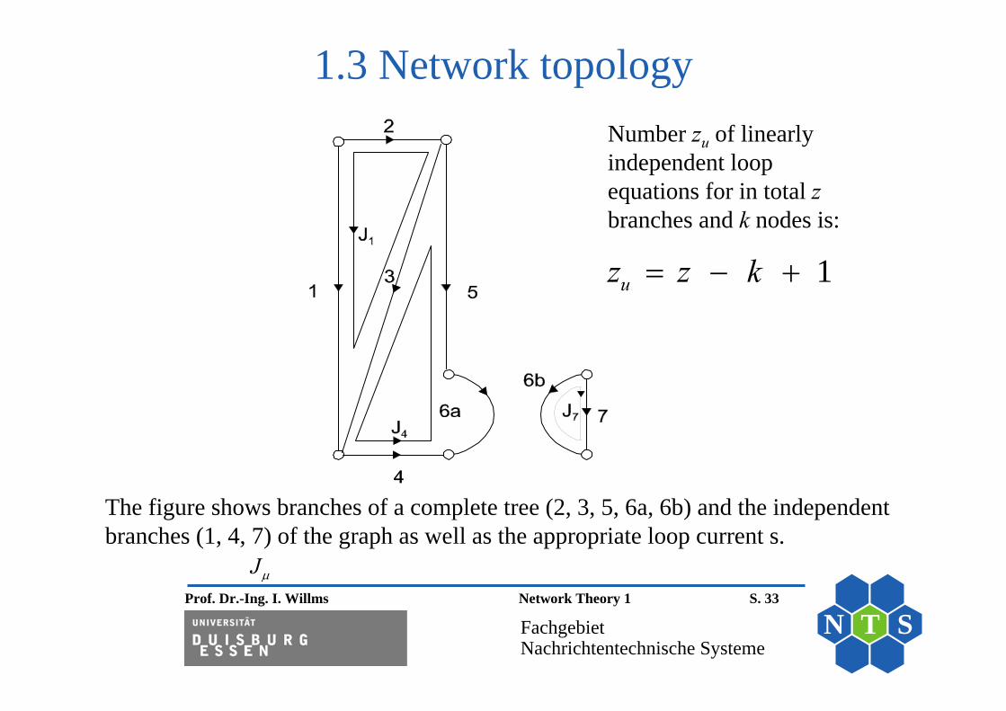
The independent branches of a network are determined by first designing a “complete tree” .
A complete tree of a connected graph is a partial graph which contains all of its nodes and some of its branches, but contains no loops.
Prof. Dr.-Ing. I. Willms Network Theory 1 S. 33
FachgebietNachrichtentechnische Systeme
N T S
1.3 Network topology
The figure shows branches of a complete tree (2, 3, 5, 6a, 6b) and the independent branches (1, 4, 7) of the graph as well as the appropriate loop current s.
J
1uz z k
Number zu of linearlyindependent loopequations for in total zbranches and k nodes is:
Prof. Dr.-Ing. I. Willms Network Theory 1 S. 34
FachgebietNachrichtentechnische Systeme
N T S
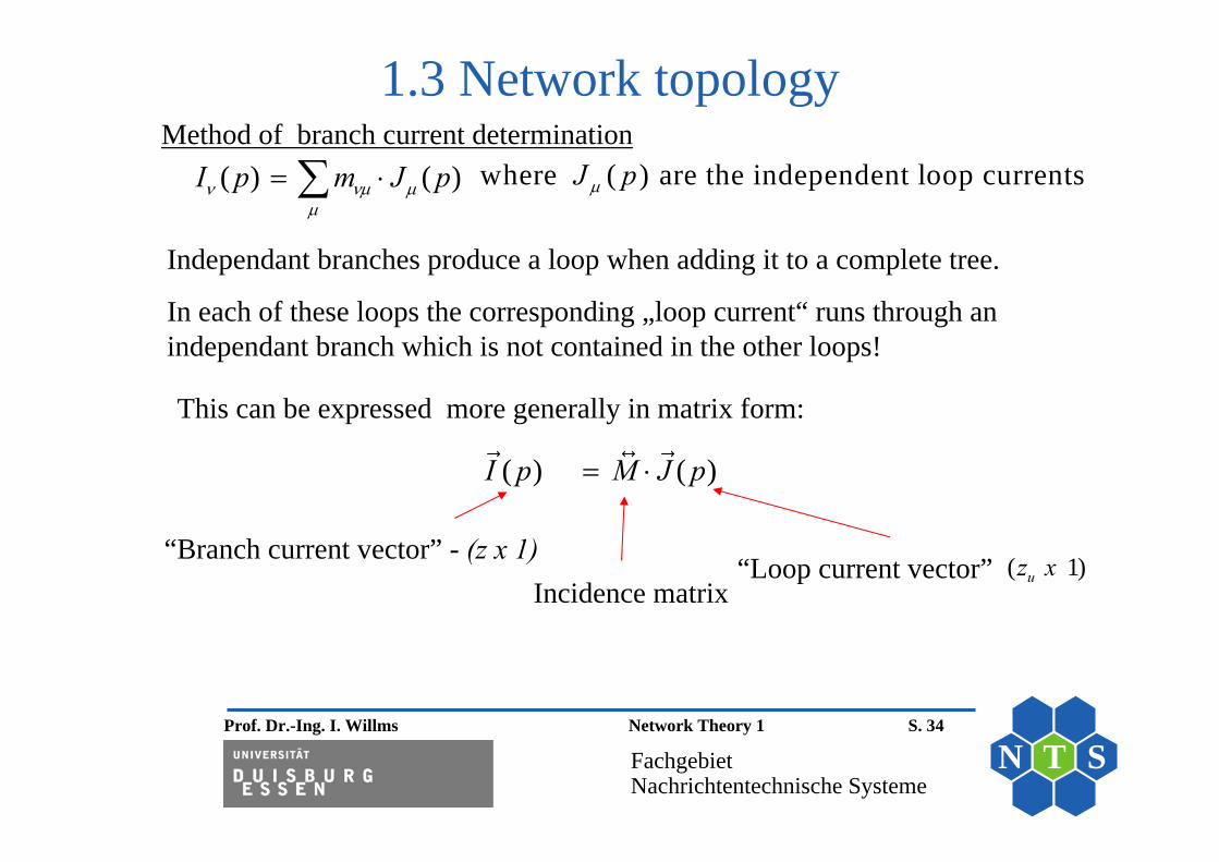
1.3 Network topologyMethod of branch current determination
( ) ( )I p m J p
where ( ) are the independent loop currentsJ p
This can be expressed more generally in matrix form:
( ) ( )I p M J p
“Branch current vector” - (z x 1)“Loop current vector” ( 1)uz x
Incidence matrix
Independant branches produce a loop when adding it to a complete tree.
In each of these loops the corresponding „loop current“ runs through an independant branch which is not contained in the other loops!

Prof. Dr.-Ing. I. Willms Network Theory 1 S. 35
FachgebietNachrichtentechnische Systeme
N T S
1.3 Network topologyIncidence matrix coefficients:
1
1
0
m
if branch v belongs to loop µ; branch and loop directions agree
if branch v belongs to loop µ; branch and loop directions do not agree
if branch v does not belong to loop µ
Kirchhoff’s voltage rule can then be formulated as
1
( ) 0 with ( ) as the voltage of the branch z
m U p U p v
Prof. Dr.-Ing. I. Willms Network Theory 1 S. 36
FachgebietNachrichtentechnische Systeme
N T S
1.3 Network topology
1( )
( ) ( )
( )z
U p
U p U p
U p
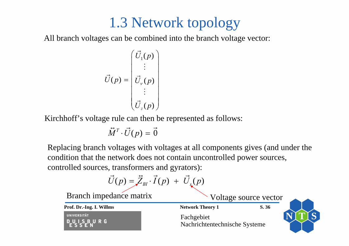
Kirchhoff’s voltage rule can then be represented as follows:
( ) 0TM U p
Replacing branch voltages with voltages at all components gives (and under the condition that the network does not contain uncontrolled power sources, controlled sources, transformers and gyrators):
( ) ( ) ( )BI sU p Z I p U p
Voltage source vectorBranch impedance matrix
All branch voltages can be combined into the branch voltage vector:

Prof. Dr.-Ing. I. Willms Network Theory 1 S. 37
FachgebietNachrichtentechnische Systeme
N T S
1.3 Network topologyBranch impedance matrix: (purely diagonally with z x z elements)
1( ) 0 00 ( ) 00 0 ( )
BI
z
Z pZ Z p
Z p

Prof. Dr.-Ing. I. Willms Network Theory 1 S. 38
FachgebietNachrichtentechnische Systeme
N T S
1.3 Network topology
( ) ( ) ( )BI sU p Z I p U p
( ) ( )I p M J p
Now the following equations will be combined:
( ) ( ) ( )BI sU p Z M J p U p
( ) ( ) ( ) 0T T TBI sM U p M Z M J p M U p
Thus the loop impedance matrix Z(p) appears:
11 12 1
21 2
1
( )
u
u
u u u
z
zTBI
z z z
Z Z Z
Z ZZ p M Z M
Z Z
They give:
Another relation results from using: ( ) 0TM U p
( )u uz x z
Prof. Dr.-Ing. I. Willms Network Theory 1 S. 39
FachgebietNachrichtentechnische Systeme
N T S
1.3 Network topology
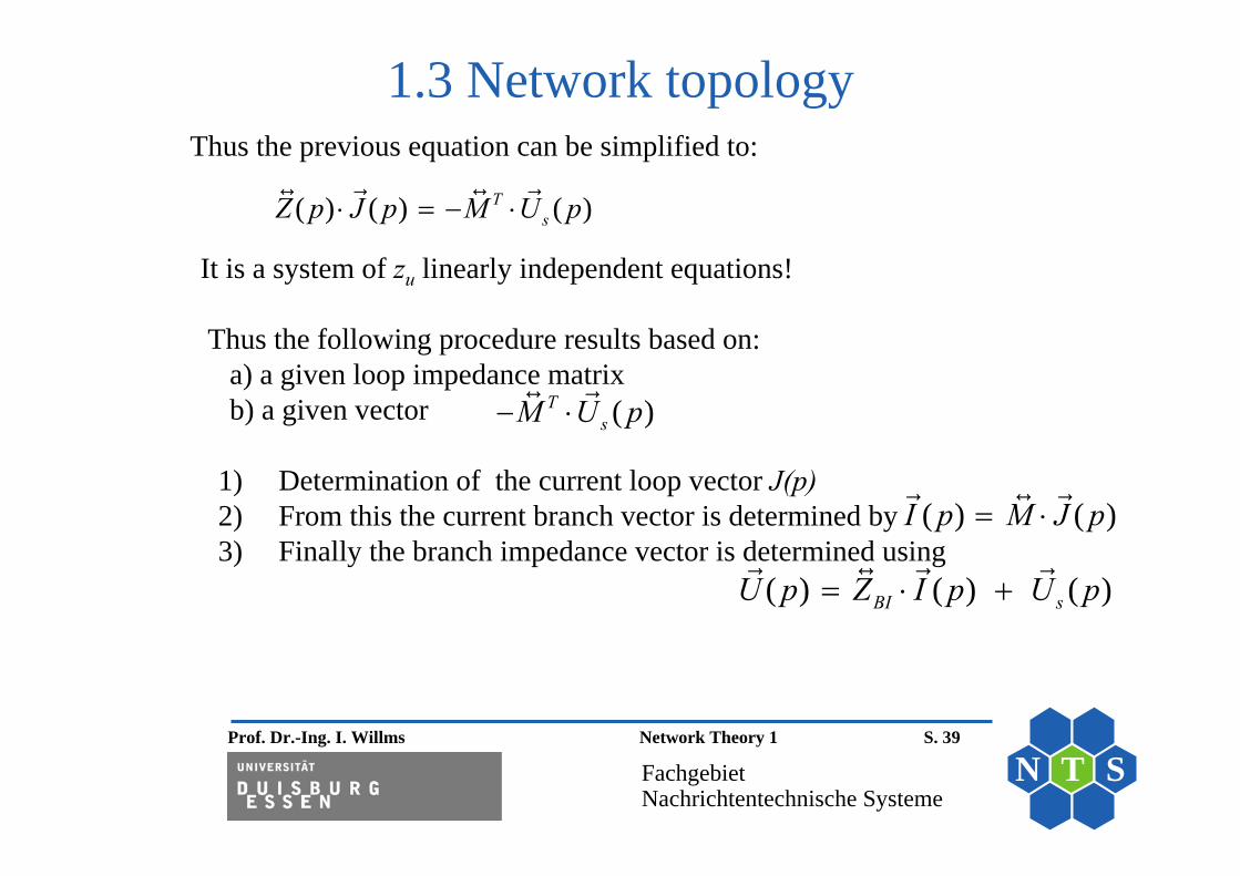
( ) ( ) ( )TsZ p J p M U p
( ) ( )I p M J p
Thus the following procedure results based on:a) a given loop impedance matrixb) a given vector
It is a system of zu linearly independent equations!
( )TsM U p
1) Determination of the current loop vector J(p)2) From this the current branch vector is determined by3) Finally the branch impedance vector is determined using
Thus the previous equation can be simplified to:
( ) ( ) ( )BI sU p Z I p U p

Prof. Dr.-Ing. I. Willms Network Theory 1 S. 40
FachgebietNachrichtentechnische Systeme
N T S
1.3 Network topology
1
1a
mif the direction of loop and at the common branch are equal
n
mIf the direction of loop and at the common branch are not equal
n
for all branches , which belong to loop
Here is the sum of all impedances in a loop.
mm m
mm
Z Z
Z
for all branches , which belong to loop and loop nm v m nZ a Z
For RLC-networks with independent voltage sources the loop impedance matrix can be set up as follows:
Prof. Dr.-Ing. I. Willms Network Theory 1 S. 41
FachgebietNachrichtentechnische Systeme
N T S
Chapter 1
Introduction
1.4 Network Functions
Prof. Dr.-Ing. I. Willms Network Theory 1 S. 42
FachgebietNachrichtentechnische Systeme
N T S
1.4 Network functions
The network function NL(p) is defined as the ratio of the Laplace transform of the response signal and the Laplace transform of the input signal under the conditions that:
1. All network elements are linear and time invariant (in short LTI or LZI)
2. All network elements are in the energyless initial condition (zero state).
If the response signal and the input signal are at the same branch, the network function is called two-terminal function or impedance function or admittance function.

Prof. Dr.-Ing. I. Willms Network Theory 1 S. 43
FachgebietNachrichtentechnische Systeme
N T S
1.4 Network functionsAn example of an impedance function:
( )( )( )
LL
L
U pZ pI p
Input and response signal of a two-port LTI system gives the network impedance function:
( )LI p ( )LU p
( )LvU p
( )LvI p
( )LvU p
Branch v
Two-terminal network
Remainder network

Prof. Dr.-Ing. I. Willms Network Theory 1 S. 44
FachgebietNachrichtentechnische Systeme
N T S
1.4 Network functionsIf the excitation signal and the response are located at different branches of the network or at different ports, then one calls the appropriate network function an effective function
An example of an effective function:
( )( )
( )L
LL
U pH p
U p
Input and the response signal of a two-port LTI network:
( )LU p ( )LU p
( )LH p
.................
.......... ...............
.. ( )LU p
( )I p( )LvI p
Branch v Branch LZI twoport(Remainder network)
( )LvU p
...............
..
..........

Prof. Dr.-Ing. I. Willms Network Theory 1 S. 45
FachgebietNachrichtentechnische Systeme
N T S
1.4 Network functionsModern network theory uses a description of the transmission characteristics of networks in a representation which follows partly that of classical network theory:
The classical representation is in time domain instead of p domain:1 ( ) cos ( )2 eff uu t U t
1 ( ) cos ( )2 eff ui t I t and
.................
.................
..........
...............
..
..........I2
IA
U2
2R
1R
U0
U1
I1
LZI-two port network

Prof. Dr.-Ing. I. Willms Network Theory 1 S. 46
FachgebietNachrichtentechnische Systeme
N T S
1.4 Network functionsFor passive networks it is reasonable to look at both voltagetransmission and current transmission through the network. This is done for a typical case with impedance matching at the input.
1
12 2
11 0
with / 2LU R R L
U U UA RU U I Voltage amplification then is:
Current amplification then is:1
2 2
1 0 1 0 1/ 2 / 2L
AI R R
I I IA
I U R U R
An operation transmission factor then can be defined:
2 2 22 2 2 12
0 0 1 0 1 0 2
/( )
/ 2 / 2 ( / 2) 1/ / 2B U I LB
I U RU U U RA A A H pU U R U R U R
The inverse of this factor leads then to the insertion loss function.

Prof. Dr.-Ing. I. Willms Network Theory 1 S. 47
FachgebietNachrichtentechnische Systeme
N T S
1.4 Network functionsDefinition of the insertion loss function: 2
00
1 22
212
2
141 2( )BD p j
B
UUR RH
A R UUR
This definition follows the idea that the magnitude of the insertion loss function can be expressed using 2 effective powers (related to the input and to the load):
Therefore here the magnitude of the insertion loss function is considered and can be rewritten using the two effective powers.
20
0 max.14
UP
R
22
22
Here voltages represent effective valuesU
PR

Prof. Dr.-Ing. I. Willms Network Theory 1 S. 48
FachgebietNachrichtentechnische Systeme
N T S
1.4 Network functions
Thus we obtain:
0max 2
22 1
12( ) o
BD
UP RHP R U
Here the two effective powers are represented by:
0 max.P The maximum effective power passed to an external load resistance attached to a voltage supply (or the input power)
(The maximum is given in case of )
LR
1LR R
2P The effective power at the load 2R
This definition of the insertion loss function is due to the fact that in early days of communications technology the transmission of telephone/telegraph signals over lossy long lines was quite an important problem.
Prof. Dr.-Ing. I. Willms Network Theory 1 S. 49
FachgebietNachrichtentechnische Systeme
N T S
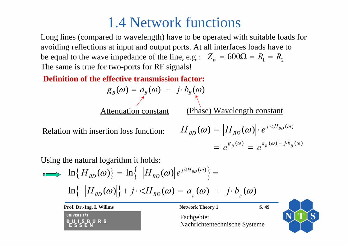
1.4 Network functionsLong lines (compared to wavelength) have to be operated with suitable loads for avoiding reflections at input and output ports. At all interfaces loads have tobe equal to the wave impedance of the line, e.g.:The same is true for two-ports for RF signals!
1 2600wZ R R
Definition of the effective transmission factor:( ) ( ) ( )B B Bg a j b
( )
( ) ( ) ( )
( ) ( ) BD
B B B
j HBD BD
g a j b
H H e
e e
Attenuation constant (Phase) Wavelength constant
Using the natural logarithm it holds:
( )ln ( ) ln ( )
ln ( ) ( ) ( ) ( )
BD
B B
j HBD BD
BD BD
H H e
H j H a j b
Relation with insertion loss function:
Prof. Dr.-Ing. I. Willms Network Theory 1 S. 50
FachgebietNachrichtentechnische Systeme
N T S
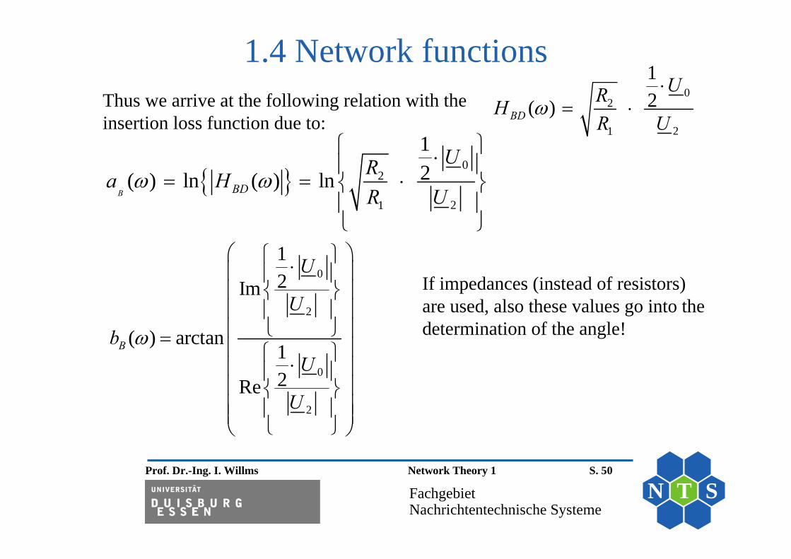
1.4 Network functions
0
2
21
12( ) ln ( ) ln
B BD
URa HR U
0
2
0
2
12Im
( ) arctan12Re
B
U
U
bU
U
Thus we arrive at the following relation with theinsertion loss function due to:
02
21
12( )BD
URHR U
If impedances (instead of resistors) are used, also these values go into thedetermination of the angle!
Prof. Dr.-Ing. I. Willms Network Theory 1 S. 51
FachgebietNachrichtentechnische Systeme
N T S
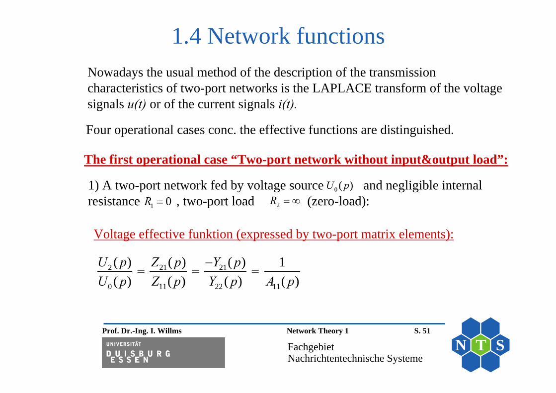
1.4 Network functionsNowadays the usual method of the description of the transmissioncharacteristics of two-port networks is the LAPLACE transform of the voltage signals u(t) or of the current signals i(t).
Four operational cases conc. the effective functions are distinguished.
The first operational case “Two-port network without input&output load”:
1) A two-port network fed by voltage source and negligible internal resistance , two-port load (zero-load):
0 ( )U p
1 0R 2R
2 21 21
0 11 22 11
( ) ( ) ( ) 1( ) ( ) ( ) ( )
U p Z p Y pU p Z p Y p A p
Voltage effective funktion (expressed by two-port matrix elements):

Prof. Dr.-Ing. I. Willms Network Theory 1 S. 52
FachgebietNachrichtentechnische Systeme
N T S
1.4 Network functions2) A two-port network fed by voltage supply source and internalresistance , two-port load and (short-circuit at output)
0 ( )U p
1 0R 2 0R 2 ( ) 0U p
Transmission admittance function:
2121
0 12
( ) ( ) 1( )( ) ( )det
AI p Z p Y pU p A pZ
3) A two-port network fed by power supply source with and internalconductance with load (open circuit).
0 ( )I p
1 1(1/ ) 0Y R 2R
2 2121
0 21
( ) ( ) 1( )( ) ( )det
U p Y pZ pI p A pY
Transmission impedance function:

Prof. Dr.-Ing. I. Willms Network Theory 1 S. 53
FachgebietNachrichtentechnische Systeme
N T S
1.4 Network functions
4) A two-port network fed by power supply source and internalconductance and (closed circuit at output).
0 ( )I p
1 1(1/ ) 0Y R 2 0R
21 21
0 22 11 22
( ) ( ) ( ) 1( ) ( ) ( ) ( )
AI p Z p Y pI p Z p Y p A p
Current effective funktion:
Prof. Dr.-Ing. I. Willms Network Theory 1 S. 54
FachgebietNachrichtentechnische Systeme
N T S
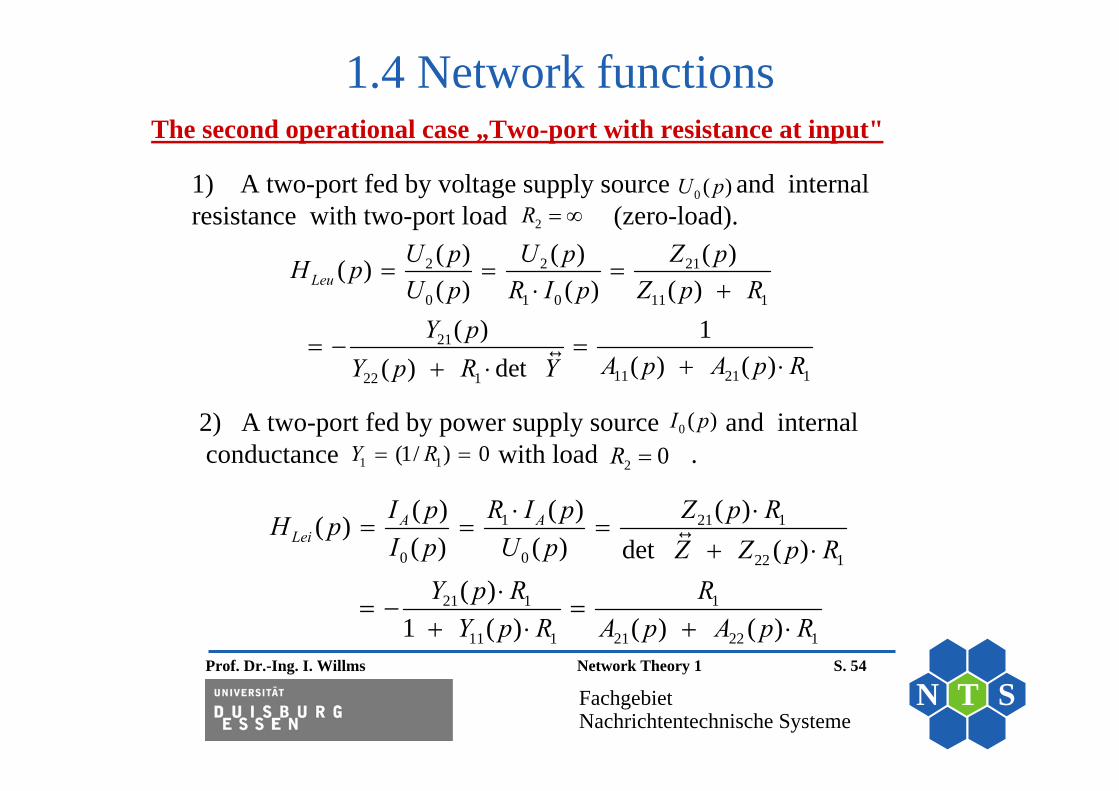
1.4 Network functions
2 2 21
0 1 0 11 1
21
11 21 122 1
( ) ( ) ( )( )( ) ( ) ( )
( ) 1( ) ( )( ) det
LeuU p U p Z pH pU p R I p Z p R
Y pA p A p RY p R Y
1 21 1
0 0 22 1
21 1 1
11 1 21 22 1
( ) ( ) ( )( )( ) ( ) det ( )
( )1 ( ) ( ) ( )
A ALei
I p R I p Z p RH pI p U p Z Z p R
Y p R RY p R A p A p R
The second operational case „Two-port with resistance at input"
1) A two-port fed by voltage supply source and internal resistance with two-port load (zero-load).
0 ( )U p2R
2) A two-port fed by power supply source and internalconductance with load .
0 ( )I p
1 1(1/ ) 0Y R 2 0R

Prof. Dr.-Ing. I. Willms Network Theory 1 S. 55
FachgebietNachrichtentechnische Systeme
N T S
1.4 Network functionsThe third operational case "two-port with output load"(load resistance is finite and nonzero)
1. A two-port fed by voltage supply source and internal resistance with two-port termination gives voltage effective function:
0 ( )U p
2R1 0R
2 2 21 2
0 0 11 2
21 2 22
22 2 12 11 2
( ) ( ) ( )( )( ) ( ) det ( )
( ) ( ) ( )1 ( ) ( ) ( )
ALau
A
U p R I p Z p RH pU p U p Z Z p R
Y p R R with I p I pY p R A p A p R
2. A two-port fed by power supply source with and internalconductance and load gives current effective function:
0 ( )I p
1 1(1/ ) 0Y R 2R
2 21
0 2 0 22 2
21
22 21 211 2
( ) ( ) ( )( )( ) ( ) ( )
( ) 1( ) ( )( ) det
ALai
I p U p Z pH pI p R I p Z p R
Y pA p A p RY p R Y
Prof. Dr.-Ing. I. Willms Network Theory 1 S. 56
FachgebietNachrichtentechnische Systeme
N T S
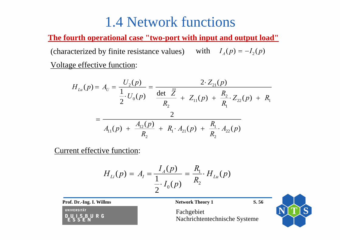
1.4 Network functionsThe fourth operational case "two-port with input and output load"
(characterized by finite resistance values)
Voltage effective function:
2 21
20 11 22 1
2 1
12 111 1 21 22
2 2
( ) 2 ( )( ) 1 det( ) ( ) ( )2
2( )( ) ( ) ( )
Lu UU p Z pH p A
RZU p Z p Z p RR R
A p RA p R A p A pR R
2( ) ( )AI p I p with
1
20
( )( ) ( )1 ( )2
ALi I Lu
I p RH p A H pRI p
Current effective function:

Prof. Dr.-Ing. I. Willms Network Theory 1 S. 57
FachgebietNachrichtentechnische Systeme
N T S
1.4 Network functions
21
2 111 22 1 2
1 21 2
2 11 111 1 2 21 22
1 21 2
( ) ( ) ( )2 ( )
det ( ) ( )
2( )( ) ( ) ( )
LB B Lu LiH p A H p H pZ p
R RZ Z p Z p R RR RR R
R A p RA p R R A p A pR RR R
Combination of corresponding current and voltage effective functionsgive the operation effective function:
The determination of the formula makes use of the the definition of AB , the relations for voltages at input and output and the two-port cascade matrix equations.

Prof. Dr.-Ing. I. Willms Network Theory 1 S. 58
FachgebietNachrichtentechnische Systeme
N T S
1.4 Network functions
Zerostate Response Signal( )
Input SignalL
LH p
L
0( )0 1
0 1
( )( )( ) ( )( ) ( )
L
MMm
imj H pm i
L LN Nn
n kn k
p pa pP pH p A H p eQ p b p p p
Each of these effective functions follows the general definition:
This is often also called “system function” or “system-driving function”.
An alternative representation is made using rational real fractions in p:
0 1..i i Mp
1..k k Np
zeros of the numerator P(p)
zeros of the denominator Q(p)
with
Prof. Dr.-Ing. I. Willms Network Theory 1 S. 59
FachgebietNachrichtentechnische Systeme
N T S
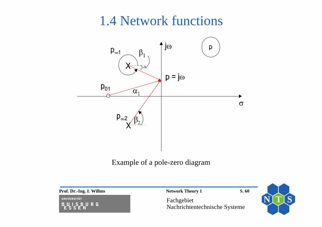
1.4 Network functions
( )0 0( ) ij p
i ip p p p e ( )( ) kj pk kp p p p e
0 1 0 2 0
1 2
( ) ML
N
p p p p p pH p A
p p p p p p
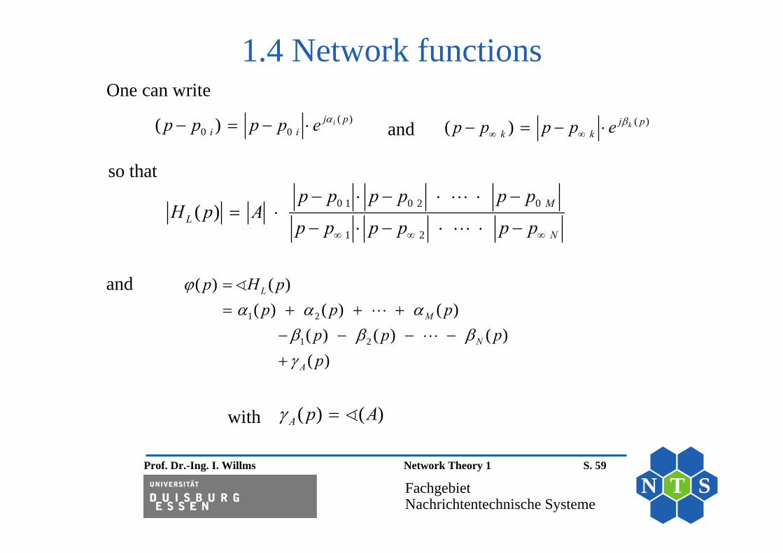
One can write
and
so that
1 2
1 2
( ) ( )( ) ( ) ( )
( ) ( ) ( )( )
L
M
N
A
p H pp p p
p p pp
and
( ) ( )A p A with
Prof. Dr.-Ing. I. Willms Network Theory 1 S. 60
FachgebietNachrichtentechnische Systeme
N T S
1.4 Network functions
Example of a pole-zero diagram
Prof. Dr.-Ing. I. Willms Network Theory 1 S. 61
FachgebietNachrichtentechnische Systeme
N T S
1.4 Network functions
( ) ( )F LH H p j
In practice, one often looks at the corresponding transfer function:
Condition: Poles of must lie in left half p plane( )LH p
In this case the following the equation holds:
0 1 0 2 0
1 2
( ) ( ) ( )( ) ( )
( ) ( ) ( )M
F LN
j p j p j pH H j A
j p j p j p
Re 0kp
Fourier transform gives the impulse response h(t) of the system!
( ) ( )F LH H j h(t) Re 0kp with
Note: This also is possible from the system function usinginverse Laplace transform!

Prof. Dr.-Ing. I. Willms Network Theory 1 S. 62
FachgebietNachrichtentechnische Systeme
N T S
1.4 Network functions
LH (p) 0M N for p
Stability of the two-port network
(with M being the order of the numerator, N being the order of the denominator)
is a condition for subsequent considerations!
1
( )( )
N
L
AH p
p p
The partial fraction method gives for
with the pole factors:
( )
( )
1 ( ) ( )( )!
NN
LNp p
dA H p p pN dp
-fold poles at location :v vN p

Prof. Dr.-Ing. I. Willms Network Theory 1 S. 63
FachgebietNachrichtentechnische Systeme
N T S
1.4 Network functions
1( )p p
sonst0
0tfüre)!1(
t tp1
sonst0
0tfüre)!1(
tA)t(h
N
1
tp1
( )LH p
With the correspondence
the impulse response h(t) thus can be determined as:
1 1
( )( 1)! ( 1)!
p t t j tt th t A e A e e

Prof. Dr.-Ing. I. Willms Network Theory 1 S. 64
FachgebietNachrichtentechnische Systeme
N T S
1.4 Network functionsThus the impulse response h(t) will satisfy the following condition
( )h t W for all t > 0 (W is a finite value)
only under the condition that:
Re 0p 1N for and
max.Re max. 0p 1)1 N for
Amplitude delimitation of h(t) corresponds to the stability definition for two-port systems.
1) In this case a special stability situation is givencharacterized by constant oszillations!
Prof. Dr.-Ing. I. Willms Network Theory 1 S. 65
FachgebietNachrichtentechnische Systeme
N T S
1.4 Network functionsStability of the system with the HURWITZ criterion:
Hurwitz – rational polynomial:
• All coefficients are real numbers
• All zeros are located in the left half of the complex p plane
The stability criterion of a two-port system thus can be expressed:
A two-port with the characteristic function or system function ( ) ( ) / ( )LH p P p Q p is stable if the denominator polynomial Q(p)
is a Hurwitz - polynomial.

Prof. Dr.-Ing. I. Willms Network Theory 1 S. 66
FachgebietNachrichtentechnische Systeme
N T S
1.4 Network functionsModified Hurwitz polynomial:
• All coefficients are real numbers• There may be simple or multiple zeros in the left half p-plane• There may be simple poles on the jω-axis but no multiple ones!
A two-port network with the system function ( ) ( ) / ( )LH p P p Q p is stable if the denominator polynomial Q(p)
is a modified Hurwitz - polynomial.

Prof. Dr.-Ing. I. Willms Network Theory 1 S. 67
FachgebietNachrichtentechnische Systeme
N T S
Chapter 1
Introduction
1.5 Two-terminal networks with special effective functions (System functions)
Prof. Dr.-Ing. I. Willms Network Theory 1 S. 68
FachgebietNachrichtentechnische Systeme
N T S
Then in addition to conjugated complex poles and zeros it holds:
1.5.1 The all-pass networkThe all-pass behaviour is defined by the system function:
( )( )( )L
Q pH p AQ p
with A being real and Q(p)being a Hurwitz - polynomial
0i kp p for corresponding i and k and the system function will be:2
0 1 22
0 1 2
' 1 2
1 2
( )( )( )
( ) ( ) ( )( ) ( ) ( )
NN
L NN
N
N
b b p b p b pQ pH p A AQ p b b p b p b pp p p p p pAp p p p p p
gives square-symmetrical pole zero configuration typical for an all-pass network

Prof. Dr.-Ing. I. Willms Network Theory 1 S. 69
FachgebietNachrichtentechnische Systeme
N T S
1.5.1 The all-pass network
1 2' '
1 2
( ) ( ) ( )( )
( ) ( ) ( )N
LN
j p j p j pH j A A
j p j p j p
For p j the corresponding transfer function gives:
Constant( )
2 1 1 2 1 1
*1,2 01,2 1,2
with ( ) ( ) and for complex conjugated poles:
and
so that here has the same distance to as = !
Fj HL FH j H e
j p j j j p j j
p j p p
A pole with the index k contributes with:
1( ) 2 arctan , 0
Nk
F kk k
H
( ) ( ) arctan( ) arctan( )k kk k k
k k
j p j j
In total it results:
A corresponding zero contributes with:( ) ( ) arctan( )k
ok k kk
j p j j
Prof. Dr.-Ing. I. Willms Network Theory 1 S. 70
FachgebietNachrichtentechnische Systeme
N T S
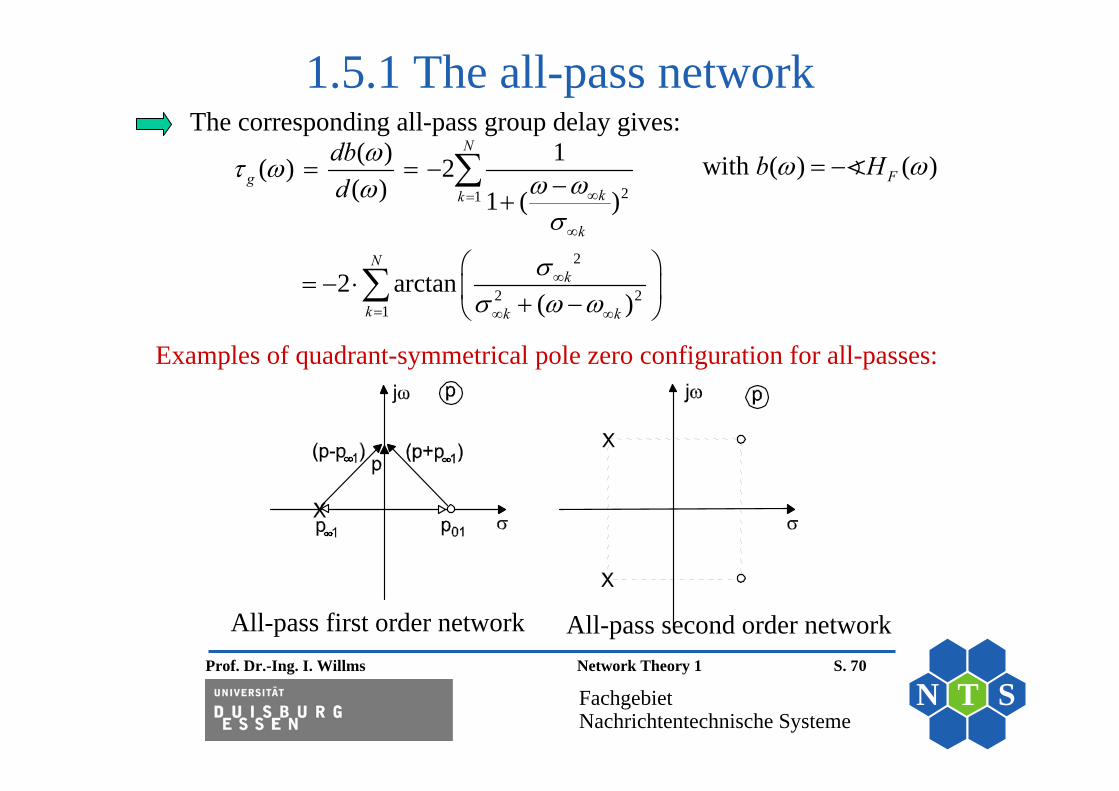
1.5.1 The all-pass network
21
2
2 21
( ) 1( ) 2( ) 1 ( )
2 arctan( )
N
gkk
k
Nk
k k k
dbd
The corresponding all-pass group delay gives:
Examples of quadrant-symmetrical pole zero configuration for all-passes:
All-pass first order network All-pass second order network
with ( ) ( )Fb H
Prof. Dr.-Ing. I. Willms Network Theory 1 S. 71
FachgebietNachrichtentechnische Systeme
N T S
1.5.1 The all-pass network
1
1
1
2
2
2
22
2
!
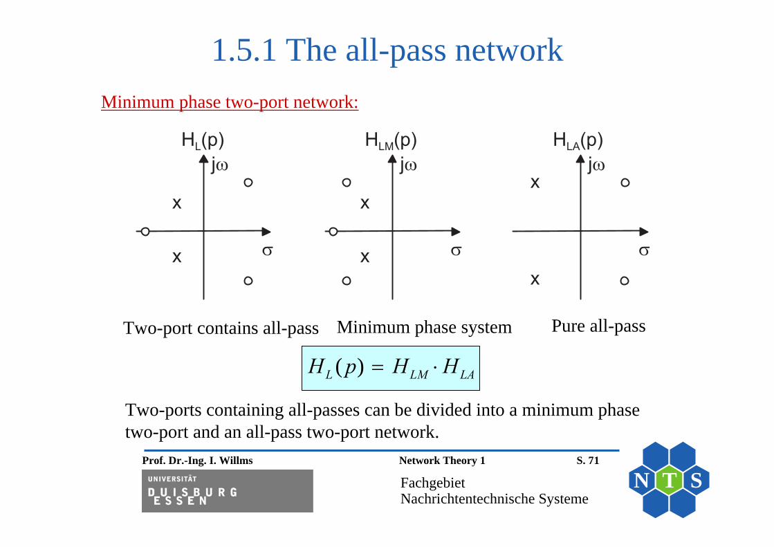
Minimum phase two-port network:
Two-port contains all-pass Minimum phase system Pure all-pass
( )L LM LAH p H H
Two-ports containing all-passes can be divided into a minimum phase two-port and an all-pass two-port network.

Prof. Dr.-Ing. I. Willms Network Theory 1 S. 72
FachgebietNachrichtentechnische Systeme
N T S
1.5.2 Bridge circuits
)
)
)
) /
'
'
)
) /
)
)
' '
*
A special two-port network with interesting properties is represented by:
Bridge connection representation Cross connection representation
Bridge network advantages: Easy synthesis relations (under conditions)
Prof. Dr.-Ing. I. Willms Network Theory 1 S. 73
FachgebietNachrichtentechnische Systeme
N T S
1.5.2 Bridge circuitsThe Z-matrix of the asymmetrical bridge two-port of previous figure:
11 12
21 22
( )( )1( )( )
a d b c b d a c
b d a c a b c da b c d
Z ZZ
Z Z
Z Z Z Z Z Z Z ZZ Z Z Z Z Z Z ZZ Z Z Z
Under the condition of and it results:a c b dZ Z Z Z
11 12
21 22
1 1( ) ( )2 21 1( ) ( )2 2
a b b a
b a b a
Z Z Z ZZ ZZ
Z Z Z Z Z Z

Prof. Dr.-Ing. I. Willms Network Theory 1 S. 74
FachgebietNachrichtentechnische Systeme
N T S
1.5.2 Bridge circuits
)
) /
' '
)
' ' )
…and the system becomes symmetric in structure:
A symmetrical bridge
Its equivalent circuit with an ideal transformer
Two conditions sufficiently and necessary for the symmetry of a two-port (exchange of the ports has no effect) are fulfilled by this circuit:
12 21Z Z
11 22Z Z

Prof. Dr.-Ing. I. Willms Network Theory 1 S. 75
FachgebietNachrichtentechnische Systeme
N T S
1.5.2 Bridge circuitsThe matrix of this symmetrical bridge two-port applies with Y
1a
a
YZ
1
bb
YZ
and
11 12
21 22
1 1( ) ( )2 21 1( ) ( )2 2
a b b a
b a b a
Y Y Y YY YY
Y Y Y Y Y Y
gives the result:
Longitudinal branch impedance aZ and transverse branch impedancebZ
are always positive real functions of p for a passive
symmetrical four-pole network!

Prof. Dr.-Ing. I. Willms Network Theory 1 S. 76
FachgebietNachrichtentechnische Systeme
N T S
1.5.2 Bridge circuitsCondition of a two-port network with symmetrical structure:
The properties of the two-port remains unchanged when exchanging the ports.
Symmetric two-ports can be transformed into equivalent circuits using thesymmetry rule of Bartlett.
1Z
2Z 2Z3Z 3Z
4Z 4Z5Z
. .
. . .
. . ..................................................
11 .2
Z 11 .2
Z
2Z 2Z
3Z 3Z
4Z 4Z52 Z 52 Z
. .
. . . .
. . . .Symmetry line
Prof. Dr.-Ing. I. Willms Network Theory 1 S. 77
FachgebietNachrichtentechnische Systeme
N T S
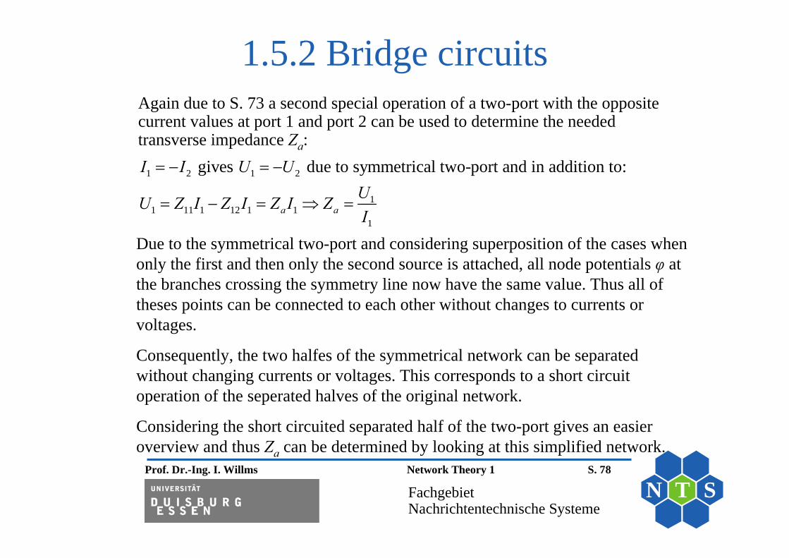
1.5.2 Bridge circuitsDue to S. 73 a special operation condition of a two-port with the same currents at both ports can be used to determine the longitudinal impedance:
1 2 1 2
11 11 1 12 1 1
1
gives due to symmetrical two-port and in addition to:
b b
I I U UUU Z I Z I Z I ZI
Due to the symmetrical two-port all node potentials φ are equal at correspondingnodes of both halfes of the two-port. Thus no current flows through branches crossingthe symmetry line. Consequently, these branches could be extracted from the networkwithout changes to currents or voltages.
Considering the two-port with extracted branches gives an easier overview and corresponds to an open circuit operation of seperated halfes of the original network.
So Zb can also be determined by looking at one separated half of the two-port in opencircuit operation.
Prof. Dr.-Ing. I. Willms Network Theory 1 S. 78
FachgebietNachrichtentechnische Systeme
N T S
1.5.2 Bridge circuits
1 2 1 2
11 11 1 12 1 1
1
gives due to symmetrical two-port and in addition to:
a a
I I U UUU Z I Z I Z I ZI
Again due to S. 73 a second special operation of a two-port with the oppositecurrent values at port 1 and port 2 can be used to determine the neededtransverse impedance Za:
Due to the symmetrical two-port and considering superposition of the cases whenonly the first and then only the second source is attached, all node potentials φ at the branches crossing the symmetry line now have the same value. Thus all of theses points can be connected to each other without changes to currents orvoltages.
Consequently, the two halfes of the symmetrical network can be separatedwithout changing currents or voltages. This corresponds to a short circuitoperation of the seperated halves of the original network.
Considering the short circuited separated half of the two-port gives an easieroverview and thus Za can be determined by looking at this simplified network.
Prof. Dr.-Ing. I. Willms Network Theory 1 S. 79
FachgebietNachrichtentechnische Systeme
N T S
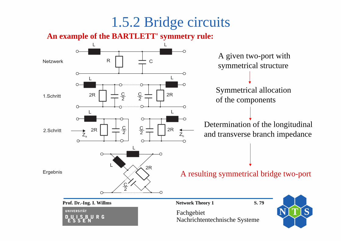
1.5.2 Bridge circuitsAn example of the BARTLETT' symmetry rule:
3 4 5 6
7
7
8 % /
$
$
$
$ $
$
) ) /
A given two-port with symmetrical structure
Symmetrical allocation of the components
Determination of the longitudinal and transverse branch impedance
A resulting symmetrical bridge two-port
Prof. Dr.-Ing. I. Willms Network Theory 1 S. 80
FachgebietNachrichtentechnische Systeme
N T S
1.5.2 Bridge circuitsNote:
• Now a network with loads is considered for determinationof relations with the operation effective function
• Method: Insertion of impedance matrix elements for a bridge network into formula for HLB(p)
• Details are shown in the next slide.

Prof. Dr.-Ing. I. Willms Network Theory 1 S. 81
FachgebietNachrichtentechnische Systeme
N T S
1.5.2 Bridge circuits21
2 111 22 1 2
1 21 2
1 2 21
2 11 1 22 1 2
11 12
21 22
2( ) ( ) ( ) =det
2 = (due to S.57)
det1 ( )2with
LB Lu Li
a b
ZH p H p H pR RZ Z Z R RR RR R
R R ZZ R Z R Z R R
Z ZZ ZZ
Z Z
2 2
1 ( )2
1 1( ) ( )2 2
1 1 and det (( ) ( ) 44 4
b a
b a b a
a b b a a b
Z Z
Z Z Z Z
Z Z Z Z Z Z Z
1 2
1 2 1 2
( ) ( )( ) 1( ) ( ) ( ) ( ) ( )
2
b aLB
a b a b
R R Z p Z pH p
Z p Z p R R Z p Z p R R
Prof. Dr.-Ing. I. Willms Network Theory 1 S. 82
FachgebietNachrichtentechnische Systeme
N T S
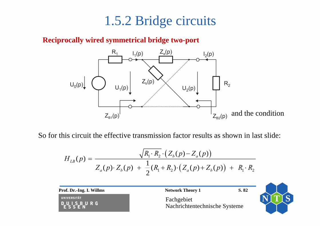
1.5.2 Bridge circuitsReciprocally wired symmetrical bridge two-port
' ' '
) 9 ) 9
) /
) $
$
1 2
1 2 1 2
( ) ( )( ) 1( ) ( ) ( ) ( ) ( )
2
b aLB
a b a b
R R Z p Z pH p
Z p Z p R R Z p Z p R R
So for this circuit the effective transmission factor results as shown in last slide:
and the condition

Prof. Dr.-Ing. I. Willms Network Theory 1 S. 83
FachgebietNachrichtentechnische Systeme
N T S
1.5.2 Bridge circuits
1 2 1 2
1 2
1 2
1 2 1 2
1 ( )( ) 2
( ) ( )( )1 ( )
2
LBa
b a
aLB
R R R R H pZ p R R
Z p Z pZ p R R H pR R R R
After solving for an easily usable relation results (for a given operation effective function and given loads):
( )bZ p
The operation impedances (input and output impedances) can be determined as:
211
1 2
2 ( ) ( ) ( ) ( )( )( )( ) 2 ( ) ( )
a b a bB
a b
Z p Z p R Z p Z pU pZ pI p R Z p Z p
0
122
2 1( ) 0
2 ( ) ( ) ( ) ( )( )( )( ) 2 ( ) ( )
a b a bB
a bU p
Z p Z p R Z p Z pU pZ pI p R Z p Z p
For the input:
For the output:
Prof. Dr.-Ing. I. Willms Network Theory 1 S. 84
FachgebietNachrichtentechnische Systeme
N T S
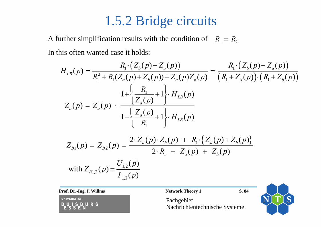
1.5.2 Bridge circuitsA further simplification results with the condition of
In this often wanted case it holds: 1 2R R
1 12
1 1 1 1
( ) ( ) ( ) ( )( )
( ( ) ( )) ( ) ( ) ( ) ( )b a b a
LBa b a b a b
R Z p Z p R Z p Z pH p
R R Z p Z p Z p Z p R Z p R Z p
1
1
1 1 ( )( )
( ) ( )( )1 1 ( )
LBa
b aa
LB
R H pZ p
Z p Z pZ p H p
R
11 2
1
1,21,2
1,2
2 ( ) ( ) ( ) ( )( ) ( )
2 ( ) ( )( )
with ( )( )
a b a bB B
a b
B
Z p Z p R Z p Z pZ p Z p
R Z p Z pU p
Z pI p

Prof. Dr.-Ing. I. Willms Network Theory 1 S. 85
FachgebietNachrichtentechnische Systeme
N T S
1.5.2 Bridge circuitsAnother simplification uses the additional condition 2
1( ) ( ) and gives:a bZ p Z p R
1
1
( )( )( )
aLB
a
R Z pH pR Z p
1
1
( )( )( )
bLB
b
Z p RH pZ p R
or
11 ( )( )1 ( )
LBa
LB
H pZ p RH p
1
1 ( )( )1 ( )
LBb
LB
H pZ p RH p
dissolving
( )bZ p as well as ( )aZ p depend only on the internal resistance and the
Operation effective function!

Prof. Dr.-Ing. I. Willms Network Theory 1 S. 86
FachgebietNachrichtentechnische Systeme
N T S
1.5.2 Bridge circuits
The conditions of realizing rational two-poles just with passive RLCÜelements are:
Im ( ) 0Z p for all p with (DC-case due to 0)p
Re ( ) 0Z p for all p with Re 0p
The last equation means that the two-pole cannot deliver energy (true forall passive two-poles)! (see also S.11 of chapter 2)
These conditions are now considered with respect to the two impedancesof the symmetric bridge circuit.
To observe:Not all effective transmission factors lead to impedances realizable just bypassive RLCÜ elements!
Prof. Dr.-Ing. I. Willms Network Theory 1 S. 87
FachgebietNachrichtentechnische Systeme
N T S
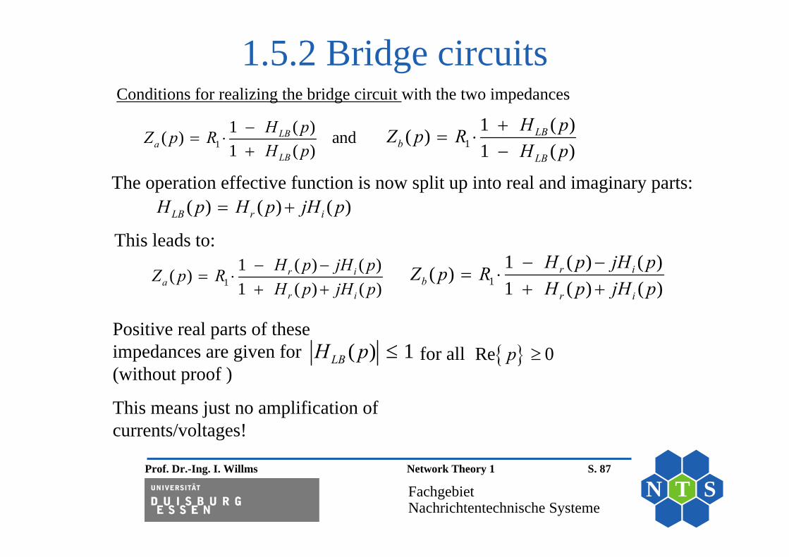
1.5.2 Bridge circuits
11 ( ) ( )( )1 ( ) ( )
r ia
r i
H p jH pZ p RH p jH p
11 ( )( )1 ( )
LBb
LB
H pZ p RH p
11 ( )( ) and1 ( )
LBa
LB
H pZ p RH p
( ) ( ) ( )LB r iH p H p jH p
This leads to:
Positive real parts of these impedances are given for (without proof )
This means just no amplification of currents/voltages!
( ) 1LBH p for all Re 0p
The operation effective function is now split up into real and imaginary parts:
11 ( ) ( )( )1 ( ) ( )
r ib
r i
H p jH pZ p RH p jH p
Conditions for realizing the bridge circuit with the two impedances

Prof. Dr.-Ing. I. Willms Network Theory 1 S. 88
FachgebietNachrichtentechnische Systeme
N T S
1.5.2 Bridge circuitsIt can also be shown that positive real parts of the bridge impedances relies on the additional conditions:
a) The operation effective function has no poles in closed positive p plane
b) It holds 1 2 1( ) ( )B BZ p Z p R
The last relation is also a condition for being able to set up a chain of bridge circuits with in some sense “effectless” or “non-reactive”connections (i.e. no reflections, no effect of a second network on HLB(p)of a first network).
Or: The load of one element in the chain thus has no negative effect on the transmission properties of the previous chain elements.
Reason: The loads of all inputs and outputs are equal to: 1 2R R
Prof. Dr.-Ing. I. Willms Network Theory 1 S. 89
FachgebietNachrichtentechnische Systeme
N T S
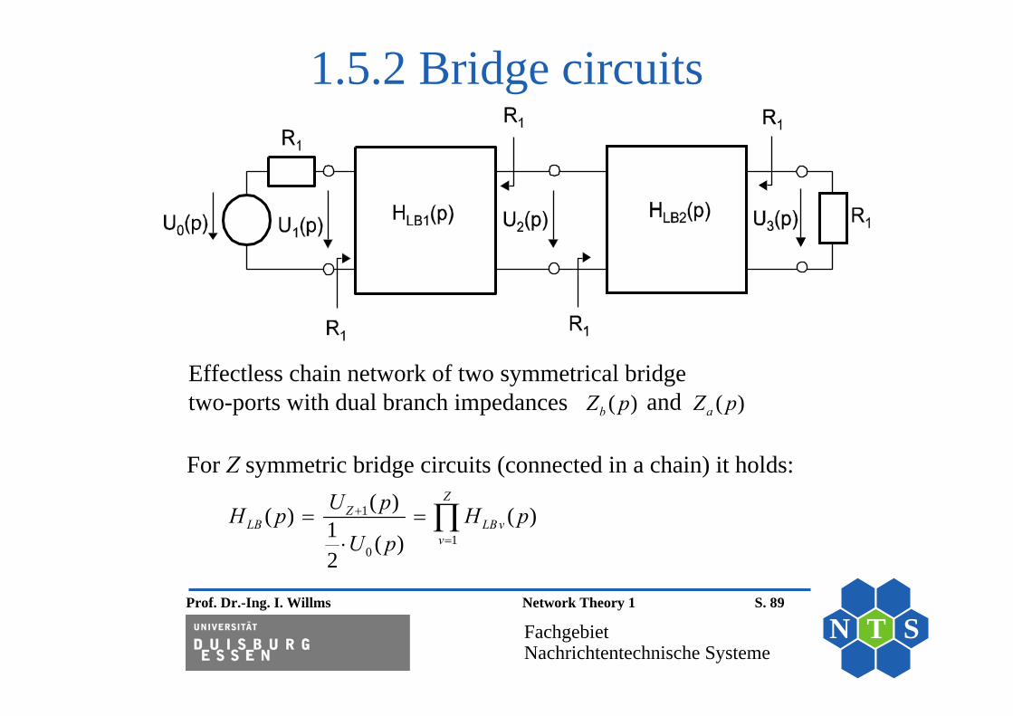
1.5.2 Bridge circuits
Effectless chain network of two symmetrical bridge two-ports with dual branch impedances ( )bZ p and ( )aZ p
1
10
( )( ) ( )1 ( )2
ZZ
LB LBvv
U pH p H pU p
For Z symmetric bridge circuits (connected in a chain) it holds:
Prof. Dr.-Ing. I. Willms Network Theory 1 S. 90
FachgebietNachrichtentechnische Systeme
N T S
1.5.2 Bridge circuits
Thus a given operation effective function can be realized using:• A number of Z chained symmetric bridge circuits• Symmetrical loads• Identical operation input and output impedances• For simplicity: Chain elements of the order of 2 (in addition to
one with the order of 1)

Prof. Dr.-Ing. I. Willms Network Theory 1 S. 91
FachgebietNachrichtentechnische Systeme
N T S
Chapter 1
Introduction
1.6 Normalization Procedures

Prof. Dr.-Ing. I. Willms Network Theory 1 S. 92
FachgebietNachrichtentechnische Systeme
N T S
1.6.1 Normalized representation of network functions
Normalization procedures help to keep the overview in a big network where usally it is hard to compare values.
Normalisations are transforms of variables using reference constants. They can be applied to frequencies and component values.
Typical normalization procedures applied to a network function N(p) might be:
• An impedance-function Z(p) is normalized
• Its argument, the complex frequency is normalized
• An operation effective function is normalized
p j

Prof. Dr.-Ing. I. Willms Network Theory 1 S. 93
FachgebietNachrichtentechnische Systeme
N T S
1.6.1 Normalized representation of network functions
N N N
p j j P
The standardizing auxiliary variable used during the frequency normalization is the normalized complex frequency:
( )nfN PN(p)Frequency normalization
( ) ( )nf NN P N P
( ) ( )nfN
pN p N
or
Prof. Dr.-Ing. I. Willms Network Theory 1 S. 94
FachgebietNachrichtentechnische Systeme
N T S
1.6.1 Normalized representation of network functions
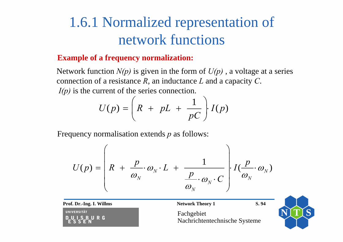
Example of a frequency normalization:
Network function N(p) is given in the form of U(p) , a voltage at a series connection of a resistance R, an inductance L and a capacity C. I(p) is the current of the series connection.
1( ) ( )U p R pL I ppC
Frequency normalisation extends p as follows:
1( ) ( )N NN N
NN
p pU p R L Ip C

Prof. Dr.-Ing. I. Willms Network Theory 1 S. 95
FachgebietNachrichtentechnische Systeme
N T S
1.6.1 Normalized representation of network functions
1( ) ( )nf N nfN
U P R P L I PP C
Thus:
( ) ( ) ( )N N nfN
pI I P I P
and
Example of the resistance normalization:This normalisation is applied to all impedance functions of the network function:
1( ) ( ) ( ) ( )U p R pL I p Z p I ppC
Impedance functions

Prof. Dr.-Ing. I. Willms Network Theory 1 S. 96
FachgebietNachrichtentechnische Systeme
N T S
1.6.1 Normalized representation of network functions
Thus the extension with NR starts with:
( ) ( )NN N
N N N
RR pLU p R R I pR R p C R
( ) ( ) ( )N nwU p R Z p I p
( ) 1 ( )nwN N N N
Z p R pLZ I pR R R p C R
After extraction of the normalization resistance from the parenthesis it results:NR
with
unitless (normalized) impedance

Prof. Dr.-Ing. I. Willms Network Theory 1 S. 97
FachgebietNachrichtentechnische Systeme
N T S
1.6.1 Normalized representation of network functions
Use of auxiliary variables in network normalizationSuch variables can be applied both to normalized voltages/currents or for Laplace transforms.
Example:( ) ( )( ) ( )nu
N N
U p I pU p Z pU U
It is possible to normalize all other elements in formulas describing network functions/elements by applying such a normalization individually!
This is called a complete normalization.

Prof. Dr.-Ing. I. Willms Network Theory 1 S. 98
FachgebietNachrichtentechnische Systeme
N T S
1.6.1 Normalized representation of network functions
An example of the complete normalization:
( ) ( )N N NN N N
N NN N N N N
N
p L R RU p R pU R Ip R CU R R
From this arises:
( )( )nuN
U pU pU
1.
NN
Rr RGR
2. Normalized resistance Normalized resistance
Voltage normalized concerning its value

Prof. Dr.-Ing. I. Willms Network Theory 1 S. 99
FachgebietNachrichtentechnische Systeme
N T S
1.6.1 Normalized representation of network functions
N
N
LlR
3. Normalized inductance
N Nc R C 4. Normalized capacity
N
pP
5. Normalized complex frequency
( ) ( )nf N NN
pI P I I P
6. Frequency normalized current
Prof. Dr.-Ing. I. Willms Network Theory 1 S. 100
FachgebietNachrichtentechnische Systeme
N T S
1.6.1 Normalized representation of network functions
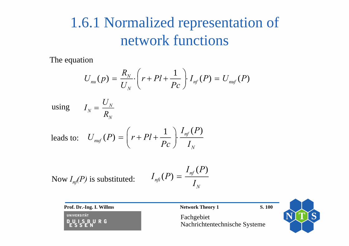
1( ) ( ) ( )Nnu nf nuf
N
RU p r Pl I P U PU Pc
The equation
using NN
N
UIR
( )1( ) nfnuf
N
I PU P r Pl
Pc I
leads to:
( )( ) nf
nfiN
I PI P
INow Inf(P) is substituted:

Prof. Dr.-Ing. I. Willms Network Theory 1 S. 101
FachgebietNachrichtentechnische Systeme
N T S
1.6.1 Normalized representation of network functions
1( ) ( )nuf nfiU P r Pl I PPc
Then the completely normalized network function results:

Prof. Dr.-Ing. I. Willms Network Theory 1 S. 102
FachgebietNachrichtentechnische Systeme
N T S
1.6.1 Normalized representation of network functions
Resistances R and conductances G appear in a network function aftera complete standardization of N(p) in the diagrams as pure numerical values.
'
$
$ 3
' 3
3
:
' :
Diagram and designation of the sizes before (left) and after the normalization (right) of the network function
Prof. Dr.-Ing. I. Willms Network Theory 1 S. 103
FachgebietNachrichtentechnische Systeme
N T S
1.6.2 Normalization in the time and frequency domain
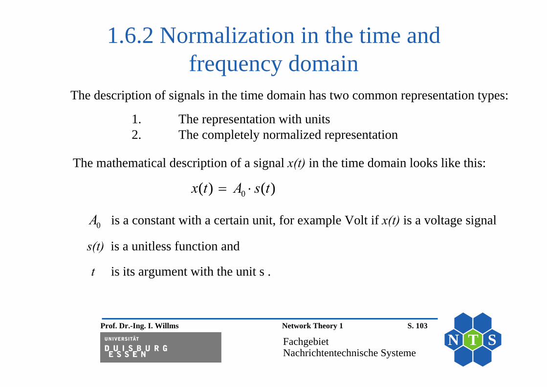
The description of signals in the time domain has two common representation types:
1. The representation with units 2. The completely normalized representation
The mathematical description of a signal x(t) in the time domain looks like this:
0( ) ( )x t A s t
0A is a constant with a certain unit, for example Volt if x(t) is a voltage signal
s(t) is a unitless function and
t is its argument with the unit s .

Prof. Dr.-Ing. I. Willms Network Theory 1 S. 104
FachgebietNachrichtentechnische Systeme
N T S
1.6.2 Normalization in the time and frequency domain
The first normalising operation leads to the dimensionless signal:
The transform of the signal representation with units into the completely standardized representation of the signal happens with the help of two standardization operations.
0( )( ) ( )nN N
Ax tx t s tA A
The second normalising operation leads to dimensionless time:
N
tT
Prof. Dr.-Ing. I. Willms Network Theory 1 S. 105
FachgebietNachrichtentechnische Systeme
N T S
1.6.2 Normalization in the time and frequency domain
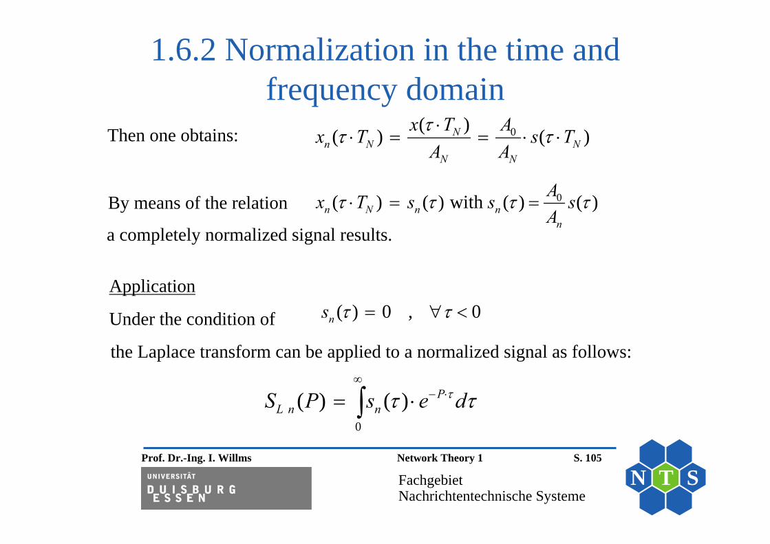
Then one obtains: 0( )( ) ( )Nn N N
N N
x T Ax T s TA A
By means of the relation 0( ) ( ) with ( ) ( )n N n nn
Ax T s s sA
a completely normalized signal results.
Application
Under the condition of ( ) 0 , 0ns
0
( ) ( ) PL n nS P s e d
the Laplace transform can be applied to a normalized signal as follows:
Prof. Dr.-Ing. I. Willms Network Theory 1 S. 106
FachgebietNachrichtentechnische Systeme
N T S
1.6.2 Normalization in the time and frequency domain
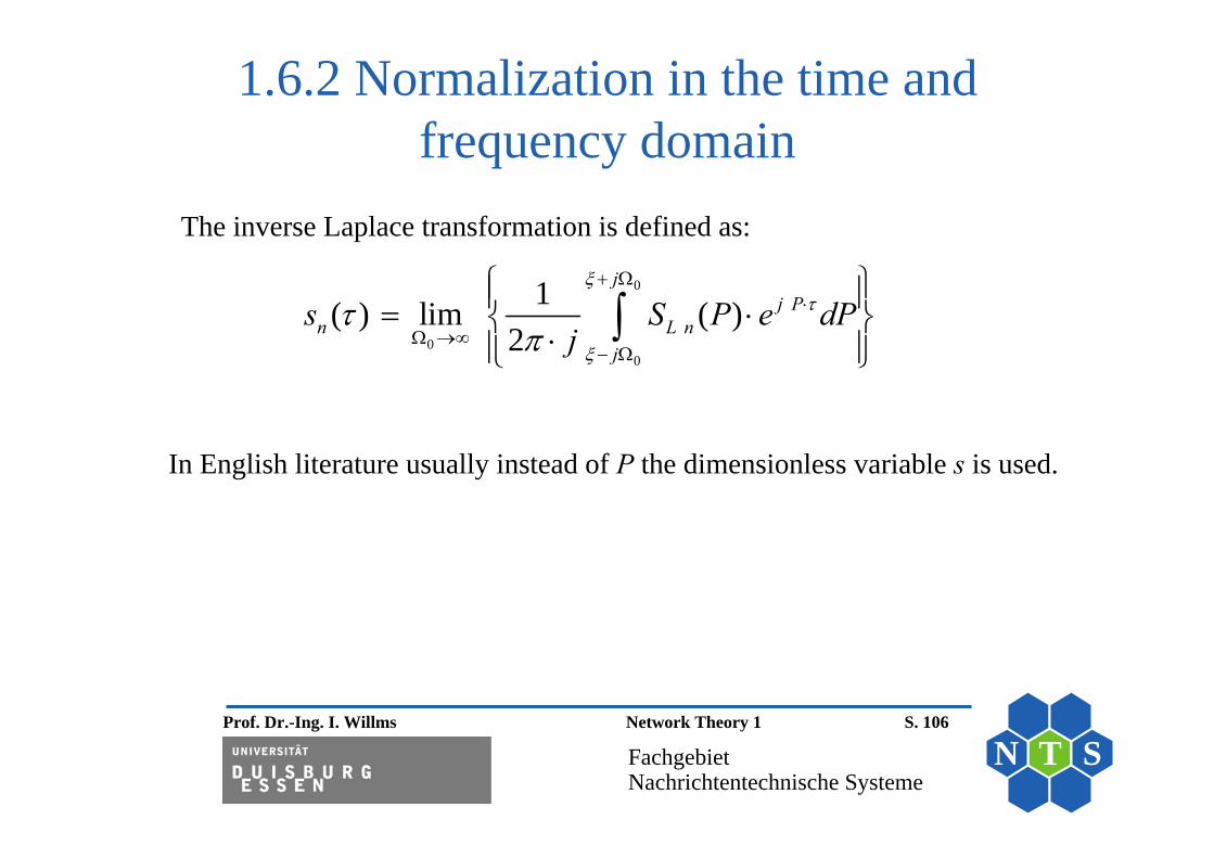
0
00
1( ) lim ( )2
jj P
n L nj
s S P e dPj
The inverse Laplace transformation is defined as:
In English literature usually instead of P the dimensionless variable s is used.
Prof. Dr.-Ing. I. Willms Network Theory 1 S. 107
FachgebietNachrichtentechnische Systeme
N T S
1.6.2 Normalization in the time and frequency domain
!
0
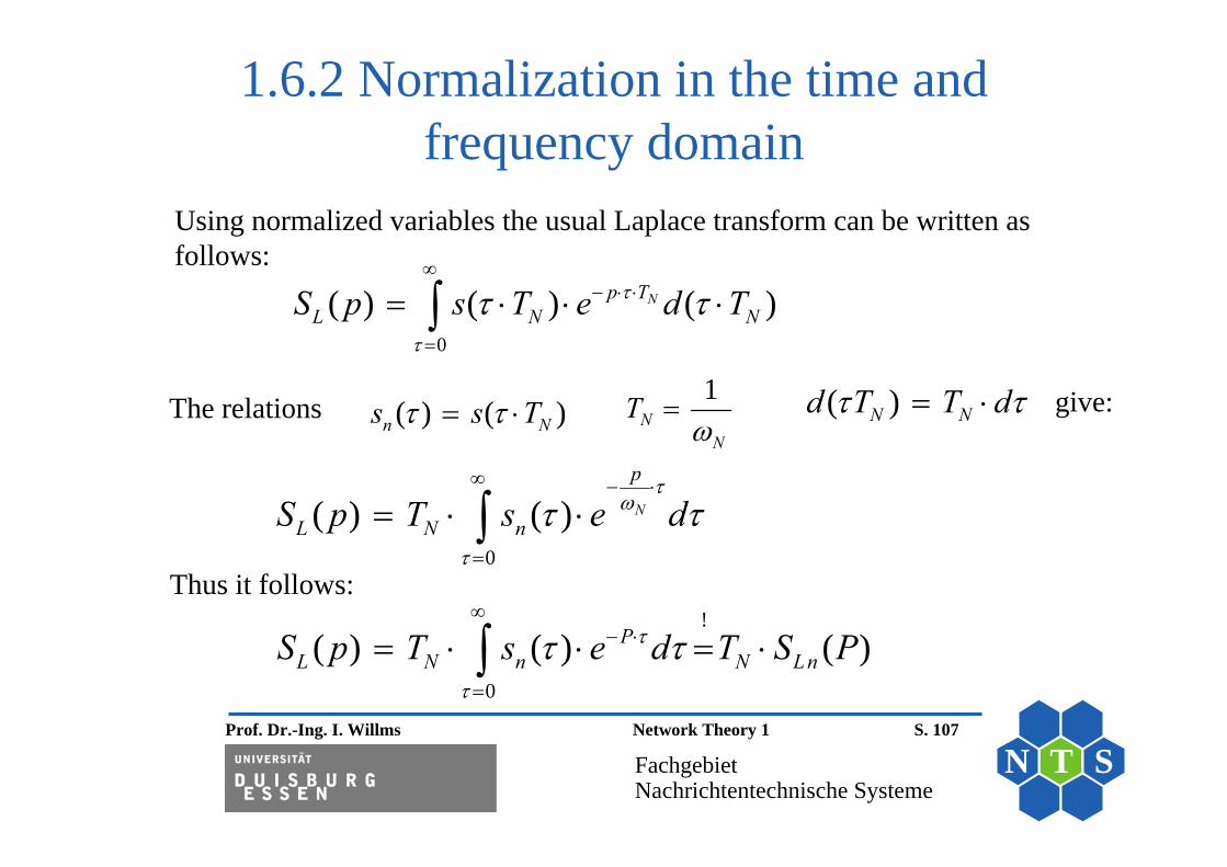
( ) ( ) ( )PL N n N LnS p T s e d T S P
0
( ) ( ) ( )Np TL N NS p s T e d T
Using normalized variables the usual Laplace transform can be written as follows:
The relations ( ) ( )n Ns s T 1
NN
T
0
( ) ( ) N
p
L N nS p T s e d
( )N Nd T T d give:
Thus it follows:
Prof. Dr.-Ing. I. Willms Network Theory 1 S. 108
FachgebietNachrichtentechnische Systeme
N T S
1.6.2 Normalization in the time and frequency domain
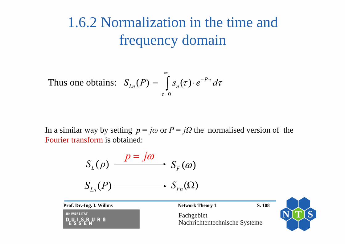
In a similar way by setting p = jω or P = jΩ the normalised version of the Fourier transform is obtained:
( )LS p ( )FS
( )LnS P ( )FnS
p j
0
Thus one obtains: ( ) ( ) PLn nS P s e d

Prof. Dr.-Ing. I. Willms Network Theory 1 S. 109
FachgebietNachrichtentechnische Systeme
N T S
1.6.2 Normalization in the time and frequency domain
( ) ( )F LS S j ( ) ( )Fn LnS S j
( ) ( ) withF N FnS T S
Thus it follows under certain restrictions:
Here the following relationships hold:
( ) ( ) j tFS s t e dt
( ) ( ) jFn nS s e d
and of course:

![U1 [] DSP: Motivation analoge ... · 30 Fouriertransformation DigitaleAudioverarbeitung Fouriertransformation, diskret siehe Matlab-Skript Signalverarbeitung [vdHeide] Digitale Audioverarbeitung](https://static.documents.pub/doc/80x56/5e55ef571c648333f70e9dc9/u1-dsp-motivation-analoge-30-fouriertransformation-digitaleaudioverarbeitung.jpg)


