Neurostereology - Wiley

NeurostereologyUnbiased Stereology of Neural Systems

COPYRIG

HTED M

ATERIAL

Background

Stereology combines mathematical and statistical approaches to estimate three-dimensional (3D) parameters of biological objects based on two-dimensional (2D) observations obtained from sec-tions through arbitrary-shaped objects (for reviews of design-based stereology, see Howard and Reed, 1998 ; Mouton, 2002, 2011 ; Evans et al., 2004 ). Among the fi rst-order parameters quantifi ed using unbiased stereology are length using plane or sphere probes, surface area using lines, volume using points, and number using the 3D disector probe. These approaches estimate stereology parameters with known precision for any object regardless of its shape.

These criteria for stereological estimation of volume and surface area are met by standard magnetic resonance imaging ( MRI ) and computed tomography ( CT ) scans, as well as tissue sec-tions separated by a known distance with systematic random sampling, that is, taking a random fi rst section followed by systematic sampling through the entire reference space ( Gundersen and Jensen, 1987 ; Regeur and Pakkenberg, 1989 ; Roberts et al., 2000 ; Mouton, 2002, 2011 ; García-Fiñana et al., 2003 ; Acer et al., 2008, 2010 ). Numerous studies have been reported using MRI to estimate brain and related volumes by stereologic and segmentation methods in adults ( Gur et al., 2002 ; Allen et al., 2003 ; Acer et al., 2007, 2008 ; Jovicich et al., 2009 ), children ( Knickmeyer et al., 2008 ), and newborns ( Anbeek et al., 2008 ; Weisenfeld and Warfi eld, 2009 ; Nisari et al., 2012 ).

The Cavalieri Principle

Named after the Italian mathematician Bonaventura Cavalieri (1598–1647), the Cavalieri principle estimates the fi rst-order parameter volume (V) from an equidistant and parallel set of 2D slices through the 3D object. As detailed later, the approach uses the area on the cut surfaces of sections through the reference space (region of interest) to estimate size (volume) of whole organs and subregions of interest. The point counting technique for area estimation uses a point-grid system superimposed with random placement onto each section through the reference space ( Gundersen and Jensen, 1987 ). The number of points falling within the reference area is counted for each section (Figure 1.1 ). Total V of a 3D object, x , is estimated by Equation 1.1 :

Stereological Estimation of Brain Volume and Surface Area from MR Images Niyazi Acer 1 and Mehmet Turgut 2 1 Department of Anatomy , Erciyes University School of Medicine , Kayseri , Turkey 2 Department of Neurosurgery , Adnan Menderes University School of Medicine , Aydın , Turkey

1

3

Neurostereology: Unbiased Stereology of Neural Systems, First Edition. Edited by Peter R. Mouton.© 2014 John Wiley & Sons, Inc. Published 2014 by John Wiley & Sons, Inc.

4 NEUROSTEREOLOGY: UNBIASED STEREOLOGY OF NEURAL SYSTEMS

V A x dxa

b

= ∫ ( ) , (1.1)

where A(x) is the area of the section of the object passing through the point x ε ( a , b ), and b is the caliper diameter of the object perpendicular to section planes. The function A ( x ) is bounded and integratable in a bounded domain ( a , b ), which represents the orthogonal linear projection of the object on the sampling axis ( García-Fiñana et al., 2003 ; Kubínová et al., 2005 ).

The Cavalieri estimator of volume is constructed from a sample of equidistant observations of f , with a distance T apart, as follows (Eq. 1.2 ):

V T f x kT T f f f fk Z

n= + = + + + +∈∑ ( ) ( ),0 1 2 3 � (1.2)

where x 0 is a uniform random variable in the interval (0, T ) and { f 1 , f 2 , . . . , f n } is the set of equi-distant observations of f at the sampling points which lie in ( a , b ). In many applications, Q rep-resents the volume of a structure, and f ( x ) is the area of the intersection between the structure and a plane that is perpendicular to a given sampling axis at the point of abscissa x ( García-Fiñana et al., 2003 ; García-Fiñana, 2006 ; García-Fiñana et al., 2009 ).

Cavalieri Principle with Point Counting

Unbiased and effi cient volume estimates with known precision ( Roberts et al., 2000 ; García-Fiñana et al., 2003 ) can be obtained from a set of parallel slices separated by a known distance ( T ), and sampled in a systematic random manner. These criteria are easily obtained from standard sets of MRI and CT scans ( Roberts et al., 2000 ; Acer et al., 2008, 2010 ).

Figure 1.1 Illustration of point counting grid overlaid on one brain section.

STEREOLOGICAL ESTIMATION OF BRAIN VOLUME AND SURFACE AREA FROM MR IMAGES 5

To apply the point-counting method, a square grid system is superimposed with random place-ment onto each Cavalieri section or slice and the number of points falling within the reference area (area of interest) counted on each section (Figure 1.1 ). Finally, an unbiased estimate of volume is calculated from Equation 1.3 :

V T a p P P P Pn= × ( ) × + + + +( ),1 2 3 � (1.3)

where n is the number of sections, P 1 , P 2 , . . . , P n show point counts, a / p represents the area associated with each test point, and T is the sectioning interval.

We used software that allowed the user to automatically sum the area of each slice and determine brain volumes by the Cavalieri principle. An unbiased estimate of volume was obtained as the sum of the estimated areas of the structure transects on consecutive systematic sections multiplied by the distance between sections, that is, V = Σ A • T . The program allowed the user to determine contrast, select true threshold value to estimate the point count automatically ( Denby et al., 2009 ).

Coeffi cient of Error ( CE ) and Confi dence Interval ( CI ) for Volume Estimation

The precision of volume estimation by the Cavalieri method was estimated by CE. Based on the original work of Matheron, the CE was adapted to the Cavalieri volume estimator by Gundersen and Jensen ( 1987 ) and more recently simplied by a number of stereologists ( Gundersen et al., 1999 ; García-Fiñana et al., 2003 ; Cruz-Orive, 2006 ; Ertekin et al., 2010 ; Hall and Ziegel, 2011 ). The CE is useful for estimating the contribution of sampling error to the overall (total) variation for stereological estimates. A pilot study of the mean CE estimate allows the user to optimize sampling parameters, for example, mean CE less than one-half of total variation; to select the appropriate number of MRI sections through the reference space; and to set the optimal density of the point or cycloid grid.

García-Fiñana ( 2006 ) pointed out that the asymptotic distribution of the parameter volume as its variance is strongly connected with the smoothness properties of the measurement function. Using the Cavalieri method, we constructed both CE and a CI value for estimation of brain volumes. The fi rst calculation involved the estimation of volume, variance of the volume estimate, and bounded intervals for the volume by Eq. (1.3) .

Second, Var ( Q T ) was estimated via Eq. (1.4) according to Kiêu ( 1997 ), which fi rst requires calculation of α ( q ), C 0 , C 1 , C 2 , and C 4 (Table 1.1 ):

Var Q q C C C T qTˆ ( ) ( ) , , .( ) = × − + ∈[ ]α 3 4 0 10 1 2

2 (1.4)

Eq. (1.5) leads to

C f f k nk i i k

i

n k

= = −+=

−

∑1

1 2 1, , , .… (1.5)

The quantities C 0 , C 1 , and C 2 can be computed from the systematic data sample ( García-Fiñana et al., 2003 ).

The smoothness constant ( q ) is then estimated from Eq. (1.6) as given in the following:

qC C C

C C C= − +

− +⎡⎣⎢

⎤⎦⎥

−⎧⎨⎩

⎫⎬⎭

max ,log

log( )

( ).0

1

2 2

3 4

3 4

1

20 2 4

0 1 2

(1.6)


The coeffi cient α ( q ) has the following expression:

α ζ ττ

( )( ) ( )cos( )

( ), , ,q

q q qq

q q= + +

−∈[ ]+ −

Γ 2 2 2 2

2 1 20 1

2 2 2 1 (1.7)

where Γ and ζ denote the gamma function and the Riemann zeta function, respectively. For fairly regular, quasi-ellipsoidal objects, q approaches 1, and for irregular objects, q approaches 0. Under these circumstances, α (0) = 0.83 and α ( 1 ) = 0.0041 ( García-Fiñana et al., 2003 ).

The bounded interval for the cerebral volume was obtained by Eq. (1.8) :

ˆ ( )( .Q mT q C C CT qλ α 3 40 1 2− + (1.8)

Note that Eq. (1.8) gives the approximate lower and upper bounds for V 2 − V 1 .

Example for Cerebral Volume, CE , and CI

Examples are provided for estimation of cerebral volume with upper and lower CI values and CE. To estimate brain volume, we used the total data set of 158 images with slice thickness 1 mm split into 15 Cavalieri planes, that is, every 10th magnetic resonance (MR) image with a different random starting point. Thus, each Cavalieri sample represents the area of cerebral cortex of a set of MR images at distance T = 10 • 1 mm = 10 mm apart (Table 1.1 ).

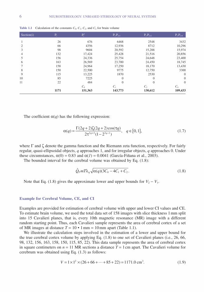
We illustrate the calculation steps involved in the estimation of a lower and upper bound for the true cerebral cortex volume by applying Eq. (1.8) to one set of Cavalieri planes (i.e., 26, 66, 98, 132, 156, 163, 158, 150, 115, 85, 22). This data sample represents the area of cerebral cortex in square centimeters on n = 11 MR sections a distance T = 1 cm apart. The Cavalieri volume for cerebrum was obtained using Eq. (1.3) as follows:

V = × × + + + + =1 1 26 66 85 22 1171 02 3( ) . .� cm (1.9)

Table 1.1 Calculation of the constants C 0 , C 1 , C 2 , and C 4 for brain volume

Section(i) P i Pi2 P i .P i + 1 P i .P i + 2 P i .P i + 4

1 26 676 6468 2548 34322 66 4356 12,936 8712 10,2963 98 9604 20,592 15,288 15,9744 132 17,424 25,428 21,516 20,8565 156 24,336 25,754 24,648 23,4006 163 26,569 23,700 24,450 18,7457 158 24,964 17,250 18,170 13,4308 150 22,500 9775 12,750 33009 115 13,225 1870 2530 0

10 85 7225 0 0 011 22 484 0 0 0

C 0 C 1 C 2 C 4 1171 151,363 143,773 130,612 109,433


C

C0

2 2 2

1

676 4356 484 151363

26 66 66 98 85 22 1454

= + + + == × + × + + × =

( )

( )

�� 889

26 98 66 132 115 22 130612

26 132 66 156 152

4

C

C

= × + × + + × == × + × + +

( )

(

�� 88 22 109433× =) .

(1.10)

The smoothness constant ( q ) is estimated from Eq. (1.6) as follows:

q = × − × +× − × +

01

2 2

3 151363 4 130612 109433

3 151363 4 145489 130,

loglog

6612

1

20 815⎡

⎣⎢⎤⎦⎥

−⎧⎨⎩

⎫⎬⎭

= . . (1.11)

Applying Eq. (1.7) with q = 0.815 leads to α ( q ) as follows:

αζ

τ( . )

( . ) ( . )cos( . . )

( ) .0 815

2 0 815 2 2 0 815 2 3 14 0 815

2 2 0 81= × + × + ×

×

Γ55 2 2 0 815 11 2

0 008+ × −−=

( ). .

. (1.12)

Therefore, the estimate of Var QT( ) obtained via Eq. (1.4) is

Var

Var

ˆ

ˆ .

Q q C C C T

Q

T

T

( ) = ( ) − +( ) ×

( ) = × × − ×

α 3 4 2

0 008 3 151363 4 1454

0 1 2

889 130612 1

22 65

2+( ) × ( )

( ) =Var ˆ . .QT

The CE for this estimate is calculated as shown in Eq. (1.13) :

CE QT( ) . / %.= =22 65 1171 4 (1.13)

Values for CI were calculated using Eq. (1.8) :

1171 3 38 22 65 1171 3 38 22 65 1154 1187

115

3

2 1

− × + ×( ) = −

− =

. . , . . , ( ) cm

V V 44 11873 3cm cm− . (1.14)

This example allowed us to identify the λ value as 3.38 according to García-Fiñana ( 2006 ). Predictive CE values were calculated using the R program using developed R codes to calculate the contribution to the predictive CE. After the initial setup and preparation of the formula, the point counts and other data were entered for each scan, and the fi nal data were obtained automati-cally using the R program (Appendix A ).

Volume Estimation Using Spatial Grid of Points

The method of volume estimation using a spatial grid of points ( Gundersen and Jensen, 1987 ; Cruz-Orive, 1997 ; Kubínová and Janácek, 2001 ) is an effi cient modifi cation of the Cavalieri principle. If a cubic spatial grid of points is applied, the object volume can be estimated by the formula (Eq. 1.15 ):

V u P= ×3 , (1.15)


where u is the grid constant (distance between two neighboring points of the grid), and P is the number of grid points falling into the object.

Using slice thickness and distance between two test points of the grid for the same value such as 1 cm leads to simple estimates of brain volume. A 1 cm × 1 cm × 1 cm grid was chosen, indicating a grid point spacing of 1 cm 3 in the plane of the image and through the depth of the volume.

Surface Area Estimation

Surface area can be estimated on vertical uniform random ( VUR ) and isotropic uniform random ( IUR ) tissue sections ( Baddeley et al., 1986 ). Estimations of surfaces require randomness of slice direction, also known as isotropy, as well as slice position ( Henery and Mayhew, 1989 ; Mayhew et al., 1996 ; Roberts et al., 2000 ).

Estimation of Surface Area Using Vertical Sections

With this approach, surface area is sampled at systematic random positions in 3D and combines the Cavalieri principle with vertical sectioning ( Baddeley et al., 1986 ), thus offering major advan-tages over earlier methods for estimation of surface area ( Mayhew et al., 1990, 1996 ).

The vertical section technique for surface area estimation uses cycloid test probes ( Baddeley et al., 1986 ). A cycloid probe is a line for which the length of arc oriented in a particular direction is proportional to the sine of the angle to vertical. The bias produced by taking VUR as opposed to IUR sections is exactly canceled by the inherent sine weighting of the orientation of the cycloid test lines; thus, IUR and VUR sections with cycloids are equivalent ( Baddeley et al., 1986 ; Gual-Arnau and Cruz-Orive, 1998 ; Gokhale et al., 2004 ).

Vertical sections are planar sections longitudinal to either a fi xed (but arbitrary) axial direction or perpendicular to a given horizontal plane. After rotating the object of interest by ø, the user cuts sections with uniform random position perpendicular to the vertical axis, thereby generating planes of fi xed distance ( T ) apart, all vertical with respect to the horizontal reference plane ( Bad-deley et al., 1986 ; Howard and Reed, 2005 ). For example, if the horizontal plane is an axial section, coronal and sagittal sections will be vertical sections ( Michel and Cruz-Orive, 1988 ; Pache et al., 1993 ). The 3D of objects is divided with uniform random position along each generating orienta-tion to form n Cavalieri series of vertical sections (Figure 1.2 a,b).

Both CT and MRI allow for sampling 3D objects into an exhaustive series of vertical sections in several systematic random orientations, each randomly offset with respect to a fi xed vertical axis ( Roberts et al., 2000 ). Thus, these data sets meet the requirement for isotropic and thus random orientations may be obtained for estimation of surface area as described previously ( Roberts et al., 2000 ; Kubínová and Janácek, 2001 ).

A random direction of the uniform random line in the fi rst orientation was selected as a random angle a from the interval (0°, 180°), then VUR sections generated a fi xed distance T apart, T = 1 cm. Starting with a 5° random angle, the direction of vertical sections in the j th segment is given by the angle aj = a 1 + ( j − 1) × (180°/ m ) ( j = 1, . . . , m ) (Figure 1.3 a–c). For example, if m = 4 and a 1 = 5°, then a 2 = 5° + 1 × (180°/4) = 50°, a 3 = 95°, a 4 = 140° (see Figure 1.3 ).

The relevant formula for estimating surface area from an exhaustive series of vertical sections was calculated from Equation 1.16 ( Roberts et al., 2000 ; Ronan et al., 2006 ; Acer et al., 2010 ):

S T a l I= × × ×2 / . (1.16)


Figure 1.2 (a) The object is fi xed horizontal plane (H), and is given isotropic rotation on the horizontal plane. (b) The object is divided with uniform random position along each generating orientation ( n = 3) to form nine Cavalieri sections of vertical section. Ø 1 = random angle (obtained in the interural π / n , n = number of orientations, T is the interval of the sections. For example, if n = 3 and Ø 1 = 20°, then Ø 2 = 20° + 1 × (180°/3) = 80°, Ø 3 = 140°.

a b Randomsystematicsampling

S

H

VV

12

34

56

7

T

89

∅1 = 20°

Φ1

Φ2

∅2 = 80°

∅

∅3 = 140°

Figure 1.3 (a) An example of four systematic orientations (if n = 4 and a 1 = 5°, then a 2 = 5° + 1 × (180°/4) = 50°, a 3 = 95°, a 4 = 140°. (b) A total of seven Cavalieri sections with slice separation (T) of 2 cm. (c) Illustration of cycloid probe overlaid on one subject all brain sections.

5°a

b

c

50° 95° 140°

We modifi ed the formula for surface area estimations of radiological images as shown in Equa-tion 1.17 :

Sn

Ta l SU

SLI= × × ×⎛

⎝⎜⎞⎠⎟ ×2 /

, (1.17)


where n is the number of random systematic orientation, a/l is the ratio of the test area to the cycloid length, T is the distance between serial sections, “ SU ” is the scale unit of the printed fi lm, “ SL ” is the measured length of the scale printed on the fi lm, and I is the number of intersections on all sections.

Eqs. ( 1.18, 1.19 ) that were used to estimate the surface area of an object by vertical sections are given in the following two formulas:

� …Sn

f f fn n1 1 2= + + +( )π ˆ ˆ ˆ (1.18)

ˆ , , , ,fa

lT I i ni ij

j

ki

= ⋅ ⋅ ⋅ ==

∑21 2

1π

… (1.19)

ˆ .

ˆ .

ˆ

f

f

f

1

2

3

21 1 457 291 109

21 1 426 271 362

21 1 389

= × × × =

= × × × =

= × × ×

π

π

π==

= × × × =

= + +

247 793

21 1 382 243 334

4291 109 271 362 247

4

1

.

ˆ .

( . .

f

Sn

ππ� .. . ) . ,793 243 334 827 0749 2+ = cm

(1.20)

where n represents the number of random systematic orientation about a central vertical axis through the object, a/l represents the ratio of test area to cycloid test length, T represents distance between Cavalieri vertical sections, I ij represent the number of intersections between cycloids and the j th vertical trace of the i th series; k i is the number of nonempty vertical sections in that series ( n = 4, T = 1 cm, a/l = 1 cm, ∑ ==i

niI1 1654):

Sn

Ta

lI I In i

i

n

i ij

i

ki

2

1 1

2= ⋅ ⋅ ⋅ == =

∑ ∑ (1.19)

ˆ

ˆ . .

S

S

n

n

2

22

2 1 1 1654

4

827 074

= × × ×

= cm

(1.21)

Four orientations were used to calculate the a/l using d = 0.637 cm. In our experiment, cycloid test lines had a 1-cm ratio of area associated with each cycloid for a/l according to Eq. 1.22 (Figure 1.4 ). In each orientation, the number of intersections on each of the MRI sections was counted on Cavalieri slices:

a l d/ /= ×π 2 (1.22)

a l/ . . / .= × =3 14 0 637 2 1 cm (1.23)

After transferring MR images to a personal computer, surface area estimation was done using different softwares. The fi rst approach required conversion of the images to analyze format using


ImageJ, which is available free from the NIH ( http://rsb.info.nih.gov/ıj ). After formatting, hdr or img fi le was opened using MRIcro ( http://www.mccauslandcenter.sc.edu/mricro/mricro/index.html ). MRIcro allows for rotation of each image for selection of random angles (Figure 1.3 ). Finally, the stereological parameters were estimated using EasyMeasure software.

Error Prediction for Surface Area for Vertical Section Method

Error prediction was divided into three processes: systematic orientations; systematic parallel sections for each orientation; and intersection counting with a cycloid test system on each section ( Cruz-Orive and Gual-Arnau, 2002 ):

(1) Var Snθ ( )�

, the variance due to n systematic orientations (2) Var Scav n( )

�, the variance due to Cavalieri vertical sections

(3) Var Scyc n( )�

, the variance due to application of cyloid probe,

where n represents the number of orientations. The CE is directly related to the variance of the surface area estimator:

CE SVar S

Sn

n

n

( )( )��

= ×100 (1.24)

CE S CE S CE S CE Sn n cav n cyc n2 2 2 2( ) ( ) ( ) ( )� � � �= + +θ (1.25)

ce S ce S ce S ce Sn cav cyc( ) ,� � � �= ( ) + ( ) + ( )θ2 2 2 (1.26)

where CE θ , CE cav and CE cyc are orientation, Cavalieri, and cycloid CE values, respectively. Although error prediction for surface area on systematic sampled images has not been previ-

ously reported in the literature, Cruz-Orive and Gual-Arnau ( 2002 ) examined precision of circular sytematic sampling and discussed error prediction formulae for the surface area estimator on verti-cal sections. For this approach based on Cruz-Orive and Gual-Arnau ( 2002 ), the variance from each level sampling in vertical section provides useful information for optimization of sample size to design at different stages for estimation of cerebral surface. The error variance var ( )� �m nS based on a global model was calculated from systematic sampling using a semicircle:

var� �m n

m n

m mm

Sr B C C

B B n nT( ) =

− −( )− ( )( ) ⋅

++

+ ++

22 2 0 1

2 2 2 22 3

2

1

ˆ ˆ ˆ

/

νˆ , , , ,νn n m≥ =2 0 1 … (1.27)

Figure 1.4 Cycloid test probe. Area per length ( a/l ) = 1 cm.

2πd

d

0.637 cml=8d

a=4πd22d


The right side of Eq. (1.27) T n2 ν estimates the local error. The constants Ĉ 0 and Ĉ 1 (Table 1.3 )

are determined by

C f f i nk i i k

i

n k

= =+=

−

∑1

1 2, , , , .… (1.28)

B 2 j ( x ) and B 2 j (0) ≡ B 2 j are a Bernoulli polynomal and number, respectively, as shown in Eq. (1.29) :

B x x x B x x x x22

44 3 21 6 2 1 30( ) , ( ) .= − + = − + − (1.29)

Choosing between the two values m = 0, 1 will typically suffi ce:

ˆˆ ˆ ˆˆ ˆ ˆ

( / )

( /D

C C

C C

B B n

B B nm

n

n

m m

m m

= − −− −

− −−

+ +

+ +

0 2

0 1

2 2 2 2

2 2 2 2

2

1

νν ))

, .n ≥ 4 (1.30)

For mB

B B n

n

nm

m m

=−

= −−

+

+ +0

1

2 2

12 2

2 2 2 2

,( / )

( ). (1.31)

For mB B n

B B n

n

nm m

m m

= −−

= −−

+ +

+ +1

2

1

4 2

12 2 2 2

2 2 2 2

2

2,

( / )

( / )

( )

( ). (1.32)

ˆˆ ˆ ˆˆ ˆ ˆ

( ), .D

C C

C C

n

nnn

n

00 2

0 1

2 2

14= − −

− −− −

−≥ν

ν (1.33)

ˆˆ ˆ ˆˆ ˆ ˆ

( )

( ), .D

C C

C C

n

nnn

n

10 2

0 1

2

2

4 2

14= − −

− −− −

−≥ν

ν (1.34)

Input m = 1 and m = 0 into Equation 1.30 and if ˆ ˆD D0 1≤ , then m = 0 and otherwise m = 1. For m = 0, 1 use following Eq. (1.27)

var max ,

var

� �

� �

0 0 1

1

06 1

2ST

nC C n

S

n n

n

( ) =−( )

× − −( )⎧⎨⎩

⎫⎬⎭

≥

(

π νˆ ˆ ˆ , ,

)) =−( )

× − −( )⎧⎨⎩

⎫⎬⎭

≥max ,030 1

20 1π νT

nC C nnˆ ˆ ˆ , .

(1.35)

We must compute νn:

ˆ .ν σn i

i

n

==

∑ 2

1

(1.36)

After computating νn, we have to calculate σi2 following Equation (1.37) . σi

2 is the variance due to Cavalieri sampling in each orientation k :

σπ

α ν νi i i ni i i na

lh q C C C2

22

0 1 22

3 4 4= ×⎛⎝⎜

⎞⎠⎟ × × ( ) × −( ) − +⎡⎣ ⎤⎦ +ˆ ˆ ˆ ˆ ˆ ii i

ki ij i j

j

n k

i

n

C I I k ni

{ } ≥

= = −+=

−

∑

, ,

ˆ , , , , .,

3

0 1 12

1

… (1.37)


We assume that the measurement function has a smoothness constant q i ∈ [0,1] that

a qq q q

qq q

( )( ) ( )cos( )

( ), , .= + +

−∈[ ]+ −

Γ 2 2 2 2

2 1 20 1

2 2 2 1

ζ ττ

(1.7)

The gamma function ( Γ ) and the Reimann zeta function ( ζ ) are tabulated and available in most mathematical software packages. In particular, α (0) = 1/12, α (1) = 1/240, α (1/2) = ζ (3)/(8 π 2 log2).

To estimate α ( q ) we need the smoothness constant q , which in turn can be estimated from the data by Kiêu–Souchet ’ s formula:

qC C C

C C C

n

n

=( )

⋅−( ) − +

−( ) − +

⎛max ,

loglog0

1

2 2

3 4

3 4

0 2 4

0 1 2

ˆ ˆ ˆ ˆ

ˆ ˆ ˆ ˆ

ν

ν⎝⎝⎜

⎞

⎠⎟ −

⎧⎨⎪

⎩⎪

⎫⎬⎪

⎭⎪≥1

27, n (1.38)

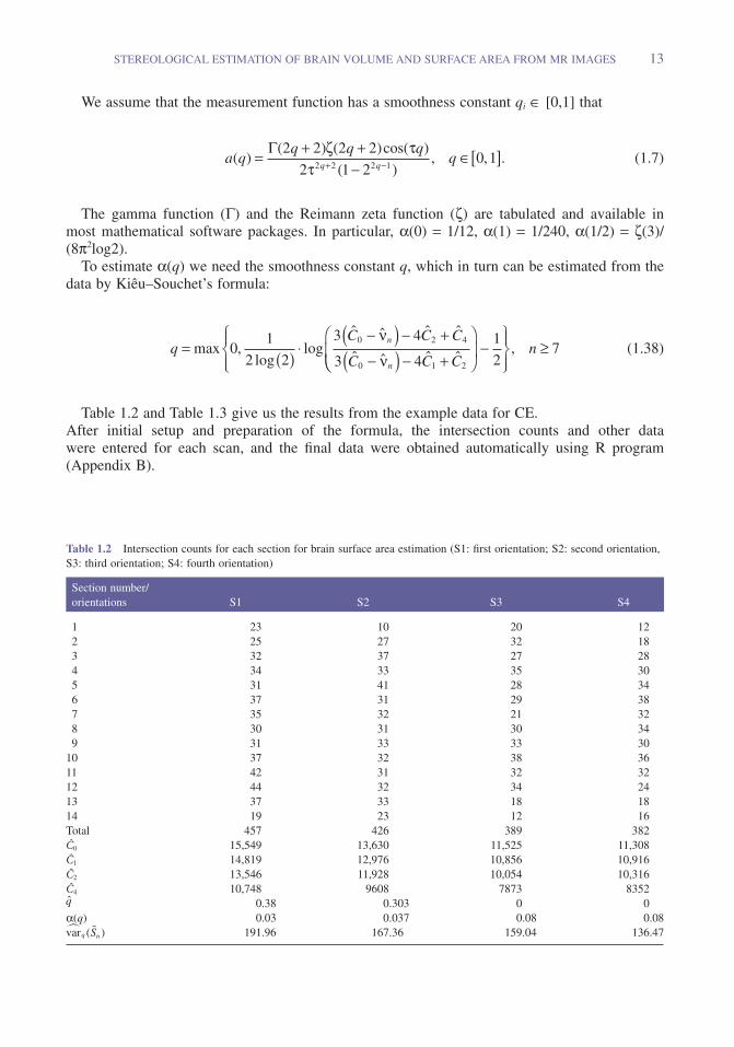
Table 1.2 and Table 1.3 give us the results from the example data for CE. After initial setup and preparation of the formula, the intersection counts and other data were entered for each scan, and the fi nal data were obtained automatically using R program (Appendix B ).

Table 1.2 Intersection counts for each section for brain surface area estimation (S1: fi rst orientation; S2: second orientation, S3: third orientation; S4: fourth orientation)

Section number/orientations S1 S2 S3 S4

1 23 10 20 122 25 27 32 183 32 37 27 284 34 33 35 305 31 41 28 346 37 31 29 387 35 32 21 328 30 31 30 349 31 33 33 30

10 37 32 38 3611 42 31 32 3212 44 32 34 2413 37 33 18 1814 19 23 12 16Total 457 426 389 382 Ĉ 0 15,549 13,630 11,525 11,308 Ĉ 1 14,819 12,976 10,856 10,916 Ĉ 2 13,546 11,928 10,054 10,316 Ĉ 4 10,748 9608 7873 8352 q 0.38 0.303 0 0 α ( q ) 0.03 0.037 0.08 0.08 var ( )� �q nS 191.96 167.36 159.04 136.47


Isotropic Cavalieri Design

According to Cruz-Orive et al. ( 2010 ), isotropic Cavalieri design has two stages:

(1) Choose a sampling axis which isotropically orients with respect to the object. (2) Take Cavalieri sections through entire the object. The sections must be systematic and paral-

lel a fi xed distance thickness ( T ) apart with a random starting interval.

We rotated MR images at random on a horizontal plan, and then cut the series exhaustively with a Cavalieri stack of sections using ImageJ (Figure 1.5 ). The result is an isotropic Cavalieri stack of sections ( Cruz-Orive et al., 2010 ).

All sections from one series were retained for the analyses, with T = 1 cm as the distance between midplane virtual slices. We used ImageJ software for surface area estimation with the following formula:

S T B B B Bn= × × + + + +( / ) ( ).4 1 2 3π � (1.39)

Let B i denote the boundary length i th planar sections:

S

S

= × × + + + + + + + +=

( / ) ( )

. .

4 1 20 42 49 62 69 98 129 112 32

915 92 3

πcm

(1.40)

Sections Analyzed with Independent Grid Design

If the section parameters cannot be measured automatically using ImageJ, then a second-stage sampling design may be applied for the estimate, as described in the following according to Cruz-Orive et al. ( 2010 ).

A given planar test grid was superimposed isotropically and uniformly at random, and indepen-dently, on each of the n sections. For each brain, the grid was superimposed uniformly at random and independently on each section.

Figure 1.6 illustrates the independent grids design with I 1 = 55, I 2 = 51, I 3 = 46, . . . , I 10 = 90. For either the independent or the registered grid designs, the unbiased estimator ˆ S in Equation 1.41 may be used with the two-stage unbiased estimator:

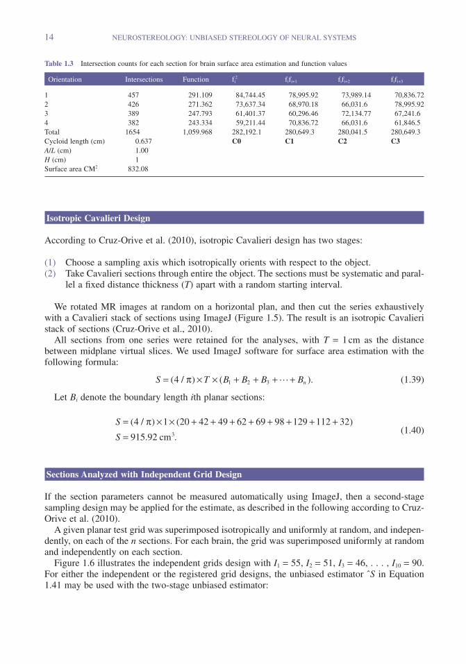
Table 1.3 Intersection counts for each section for brain surface area estimation and function values

Orientation Intersections Function fi2 f i f i + 1 f i f i + 2 f i f i + 3

1 457 291.109 84,744.45 78,995.92 73,989.14 70,836.722 426 271.362 73,637.34 68,970.18 66,031.6 78,995.923 389 247.793 61,401.37 60,296.46 72,134.77 67,241.64 382 243.334 59,211.44 70,836.72 66,031.6 61,846.5Total 1654 1,059.968 282,192.1 280,649.3 280,041.5 280,649.3Cycloid length (cm) 0.637 C0 C1 C2 C3 A / L (cm) 1.00 H (cm) 1Surface area CM 2 832.08


Figure 1.5 Isotropic Cavalieri sections.

S T d I I I In= × × + + + +( )1 2 3 � (1.41)

S

S

= × × + + + + + + + + +=

1 1 55 51 46 59 91 75 86 75 104 90

722 2

( )

.cm (1.42)

A simple formula for variance of the surface area estimate was used according to Cruz-Orive et al. ( 2010 ):

Var V ST STd

V ST

E ( )

var( ) .

�

�

= × + ( ) +⎛⎝⎜

⎞⎠⎟

=

π ζπ360

1

4

3

2

1

6

0 008727

42

3

44 30 056891+ . .STd

(1.43)


Figure 1.6 Independent grid design.

Surface Area Using the Invariator

The object of interest is a nonvoid, compact, and nonrandom subset Y of 3D Euclidean space with a piecewise smooth boundary ∂ Y . The target parameters are the surface area S ( ∂ Y ) and the volume V ( Y ) of Y . The classical construction of a motion invariant test line in 3D consists of choosing fi rst a “pivotal” plane and then a motion invariant point z in this plane. Finally, a straight line normal to the pivotal plane through the point z is a motion invariant test line. The point z may be replaced with an IUR grid of points on the pivotal plane, as described by Cruz-Orive ( 2008 ). If a test line is drawn through each point of the grid and normal to the pivotal plane, the result is an IUR, the so-called unbounded “fakir probe” ( Cruz-Orive, 1997 ; Cruz-Orive et al., 2010 ), a motion invariant test line in 3D. Using this construction to a uniform random grid of points in the pivotal plane, a “pivotal tessellation” is obtained ( Cruz-Orive, 2009 ).

Figure 1.7 a,b illustrates the unbiased estimation of the total surface area of the union of one section embedded in a ball with the invariator. In Figure 1.7 a the equatorial pivotal section plane is isotropic around the ball center. The mentioned equatorial plane is shown in Figure 1.7 a with


a square grid of points superimposed on it. The grid has to be uniformly random, namely, the pivotal point must be uniformly random relative to a basic tile of the grid. Upon this grid, the corresponding invariator grid of test lines is constructed, and the raw data are then collected (Figure 1.7 b). The estimators given by Equation (1.44) remain unbiased because the lines of the invariator grid are, in effect, motion invariant in 3D ( Cruz-Orive et al., 2010 ).

S a I= × ×2 , (1.44)

where a denotes the area of the fundamental tile of the grid (Figure 1.7 b), and I is the (random) total number of intersections between the boundary ∂ Y ( Cruz-Orive et al., 2010 ).

The obvious advantage of this method is that the resulting probe may be applied on a pivotal section using a 2D device ( Cruz-Orive et al., 2010 ).

We considered a new method to estimate surface area of variance according to Cruz-Orive et al. ( 2010 ). The mean for the object of var( s/S ) can be estimated following the formula

mean s S s Svar( / ) var( ) var( ),{ } = − � (1.45)

where var( s ) is the observed sample variance among the r invariator estimators, whereas var( )�S refers to the observable sample variance ( S ) among the r accurate estimators ( Cruz-Orive et al., 2010 ).

Volume and Surface Area Estimation Using Segmentation Method

The parameters of volume and surface area for cortical brain may be calculated using segmented images in combination with semiautomatic and automatic techniques such as the Fuzzy C-Means ( FCM ) algorithms. We used MATLAB software for segmenting MR images into parenchyma for brain volume and the surrounding line for the surface area of the cortex. After preprocessing

Figure 1.7 Invariator. (a) Construction of a p -line with respect to O through a uniform random point z in an isotropic equatorial section and randomly hitting point counting grid. (b) Invariator grid is superimposed for brain section.

a

a

Z

b


(masking), the image matrix size was reduced, and segmentation was carried out using the FCM algorithm ( Suckling et al., 1999 ; Mohamed et al., 2002 ; Tosun et al., 2004 ; Yu-Shen et al., 2010 ).

For calculation of total brain volume, the original brain image was converted to binary format. After defi ning a disc-shaped strell, morphological erode-and-dilate operations were performed and edge detection applied and collected with original brain image. The arithmetic process was done by fi lling in the area of brain as white such that only the brain region appears in the image. Finally, brain volume was obtained from the calculated area of each brain cross section.

Discussion

The Cavalieri principle has been frequently applied to the estimation of total intracranial volume, total brain volume, hippocampus, thalamus, and ventricles volume on MR images ( Roberts et al., 2000 ; Keller et al., 2002, 2012 ; Ronan et al., 2006 ; Acer et al., 2007, 2008, 2011 ; Bas et al., 2009 ; Denby et al., 2009 ; Keller and Roberts, 2009 ). Many different methods exist for estimating brain volume using manual, semiautomated, and automated techniques. Manual approaches such as stereology are considered gold standard because it is assumed that human knowledge and percep-tion is superior to computer algorithms that determine regional brain boundaries ( Keller et al., 2012 ). However, manual segmentation is tedious, requires experiment and high attention to detail, and in many cases returns results with low interrater reliability.

As an alternative to manual approaches, automatic segmentation combined with the Cavalieri-point counting estimator has been widely applied to estimate volume of internal brain compart-ments, such as cerebellum, ventricle, and so on ( Keller et al., 2002, 2012 ; Acer et al., 2007, 2008 ; Bas et al., 2009 ; Keller and Roberts, 2009 ). To assist in these procedures, various image analysis techniques have been developed in recent years to estimate the brain volume and surface area using automated and semiautomated segmentation algorithms, including freely available approaches for MR images ( Fischl et al., 1999 ; Rajendra et al., 2009 ). Of these approaches, two popular fully automated segmentation and quantifi cation software tools exist in the public domain. FreeSurfer performs subcortical and cortical segmentation and assigns a neuroanatomical label to each voxel based on probabilistic information automatically estimated from a large training set of expert measurements ( Fischl et al., 2002 ). The second option, FSL/FIRST, performs subcortical segmentation using Bayesian shape and appearance models.

Fully automatic methods require minimal training and provide highly reproducible results for the same data. The disadvantage, however, is that fully automatic approaches do not allow for human intervention or manipulation, as well as place severe limits on choices available to users performing the segmentation. As a result of these limitations, semiautomatic methods have become the preferred approach for medical image segmentation ( Keller and Roberts, 2009 ).

Semiautomatic segmentation can be divided into two major categories: region-based (region growing, region merging) and boundary-based techniques ( Kevin et al., 2009 ). One example used the Cavalieri-point counting method of design-based stereology to estimate volume for a range of organs such as liver, prostate, and others ( Sahin and Ergur, 2006 ; Acer et al., 2011 ). Stereology has been shown to be at least as precise as tracing and thresholding volumetry techniques and substantially more time effi cient than other semiautomated techniques ( Gundersen et al., 1981 ; Keller et al., 2012 ).

Quantifi cation of brain MR image data using a semiautomated threshold has also been carried out using ImageJ, a public domain image processing and analysis package developed at the National Institutes of Health ( NIH ) software for scientifi c and medical usage. This software can be used to automatically measure areas of user-defi ned ROIs on MR sections according to


the contrast and brightness of thresholded grayscale images. The segmented ROIs may be auto-matically exported to an Excel fi le with fi nal volume calculated as the product of the area and the MRI slice thickness.

For isolated objects and individual particles embedded in a solid material, the invariator ( Cruz-Orive, 2005 ) may be used to estimate surface area, membrane thickness, and volume, and elimi-nates the need for 3D scanning ( Cruz-Orive, 2011 ). Although Cruz-Orive et al. ( 2010 ) demonstrated the invariator for small isolated or embedded objects such as estimation of the external surface and the volume of rat brains, there is no study for nonembedded objects.

In conclusion, we provide examples of point counting and vertical sectioning, isotropic Cava-lieri, independent grid design, and invariator applications for the estimation of fi rst-order param-eter volume and surface area from MR images through human brains. Second, a new CE estimation procedure is given for brain surface using the vertical section design. These studies indicate that counting approximately 400–500 cycloid–brain surface intersections on 14 systematically sampled MR sections with 10-mm section thickness results in a reliable surface area estimate with a CE below 5%.

References

Acer , N. , Sahin , B. , Ba ş , O. , Ertekin , T. , Usanmaz , M. 2007 . Comparison of three methods for the estimation of total intracranial volume: stereologic, planimetric, and anthropometric approaches . Ann Plast Surg 58 ( 1 ): 48 – 53 .

Acer , N. , Sahin , B. , Usanmaz , M. , Tato ğ lu , H. , Irmak , Z. 2008 . Comparison of point counting and planimetry methods for the assessment of cerebellar volume in human using magnetic resonance imaging: a stereological study . Surg Radiol Anat 30 ( 4 ): 335 – 339 .

Acer , N. , Cankaya , M. N. , I ş çi , O. , Ba ş , O. , Camurdano ğ lu , M. , Turgut , M. 2010 . Estimation of cerebral surface area using verti-cal sectioning and magnetic resonance imaging: a stereological study . Brain Res 1310 : 29 – 36 .

Acer , N. , Turgut , A. , Özsunar , Y. , Turgut , M. 2011 . Quantifi cation of volumetric changes of brain in neurodegenerative diseases using magnetic resonance imaging and stereology . In Neurodegenerative Diseases—Processes Prevention, Protection and Monitoring , edited by R. C. Chung Chang , pp. 1 – 26 . Rijeka : InTech Open Access Publisher .

Allen , J. S. , Damasio , H. , Grabowski , T. J. , Bruss , J. , Zhang , W. 2003 . Sexual dimorphism and asymmetries in the gray-white composition of the human cerebrum . Neuroimage 18 ( 4 ): 880 – 894 .

Anbeek , P. , Vincken , L. , Floris , K. , Koeman , G. , Osch , A. , Matthias , J. P. , Grond , J. V. 2008 . Probabilistic brain tissue segmenta-tion in neonatal magnetic resonance imaging . Pediatr Res 63 : 158 – 163 .

Baddeley , A. J. , Gundersen , H. J. G. , Cruz-Orive , L. M. 1986 . Estimation of surface area from vertical sections . J Microsc 142 ( 3 ): 259 – 276 .

Bas , O. , Acer , N. , Mas , N. , Karabekir , H. S. , Kusbeci , O. Y. , Sahin , B. 2009 . Stereological evaluation of the volume and volume fraction of intracranial structures in magnetic resonance images of patients with Alzheimer ’ s disease . Ann Anat 191 : 186 – 195 .

Cruz-Orive , L. M. 1997 . Stereology of single objects . J Microsc 186 : 93 – 107 . Cruz-Orive , L. M. 2005 . A new stereological principle for test lines in three-dimensional space . J Microsc 219 : 18 – 28 . Cruz-Orive , L. M. 2006 . A general variance predictor for Cavalieri slices . J Microsc 222 ( 3 ): 158 – 165 . Cruz-Orive , L. M. 2008 . Comparative precision of the pivotal estimators of particle size . J Microsc 27 : 17 – 22 . Cruz-Orive , L. M. 2009 . The pivotal tessellation . Image Anal Stereol 28 : 101 – 105 . Cruz-Orive , L. M. 2011 . Flowers and wedges for the stereology of particles . J Microsc 243 ( 1 ): 86 – 102 . Cruz-Orive , L. M. , Gual-Arnau , X. 2002 . Precision of circular systematic sampling . J Microsc 207 : 225 – 242 . Cruz-Orive , L. M. , Ramos-Herrera , M. L. , Artacho-Pérula , E. 2010 . Stereology of isolated objects with the invariator . J Microsc

240 ( 2 ): 94 – 110 . Denby , C. E. , Vann , S. D. , Tsivilis , D. , Aggleton , J. P. , Montaldi , D. , Roberts , N. , Mayes , A. R. 2009 . The frequency and extent

of mammillary body atrophy associated with surgical removal of a colloid cyst . AJNR Am J Neuroradiol 30 : 736 – 743 . Ertekin , T. , Acer , N. , Turgut , A. T. , Aycan , K. , Ozçelik , O. , Turgut , M. 2010 . Comparison of three methods for the estimation

of the pituitary gland volume using magnetic resonance imaging: a stereological study . Pituitary 14 ( 1 ): 31 – 38 . Evans , S. M. , Janson , A. M. , Nyengaard , J. 2004 . Quantitative methods . In Neuroscience: A Neuroanatomical Approach , edited

by S. M. Evans , A. M. Janson , and J. R. Nyengaard . Cary, NC : Oxford University Press . Fischl , B. , Sereno , M. I. , Dale , A. M. 1999 . Cortical surface-based analysis. II: Infl ation, fl attening, and a surface-based coordinate

system . Neuroimage 9 ( 2 ): 195 – 207 .


Fischl , B. , Salat , D. H. , Busa , E. , Albert , M. , Dieterich , M. , Haselgrove , C. , van der Kouwe , A. , Killiany , R. , Kennedy , D. , Klaveness , S. , Montillo , A. , Makris , N. , Rosen , B. , Dale , A. M. 2002 . Whole brain segmentation: automated labeling of neuroanatomical structures in the human brain . Neuron 33 ( 3 ): 341 – 355 .

García-Fiñana , M. 2006 . Confi dence intervals in Cavalieri sampling . J Microsc 222 ( 3 ): 146 – 157 . García-Fiñana , M. , Cruz-Orive , L. M. , Mackay , C. E. , Pakkenberg , B. , Roberts , N. 2003 . Comparison of MR imaging against

physical sectioning to estimate the volume of human cerebral compartments . Neuroimage 18 ( 2 ): 505 – 516 . García-Fiñana , M. , Keller , S. S. , Roberts , N. 2009 . Confi dence intervals for the volume of brain structures in Cavalieri sampling

with local errors . J Neurosci Methods 179 ( 1 ): 71 – 77 . Gokhale , A. M. , Evans , R. A. , Mackes , J. L. , Mouton , P. R. 2004 . Design-based estimation of surface area in thick tissue sections

of arbitrary orientation using virtual cycloids . J Microsc 216 : 25 – 31 . Gual Arnau , X. , Cruz-Orive , L. M. 1998 . Variance prediction under systematic sampling with geometric probes . Adv Appl Prob

30 : 889 – 903 . Gundersen , H. J. G. , Jensen , E. B. V. 1987 . The effi ciency of systematic sampling in stereology and its prediction . J Microsc

147 ( 3 ): 229 – 263 . Gundersen , H. J. G. , Boysen , M. , Reith , A. 1981 . Comparison of semiautomatic digitizer-tablet and simple point counting per-

formance in morphometry . Virchows Arch B Cell Pathol Incl Mol Pathol 37 ( 3 ): 317 – 325 . Gundersen , H. J. G. , Jensen , E. B. V. , Kieu , K. , Nielsen , J. 1999 . The effi ciency of systematic sampling in stereology—

reconsidered . J Microsc 193 : 199 – 211 . Gur , R. C. , Gunning-Dixon , F. , Bilker , W. B. , Gur , R. E. 2002 . Sex differences in temporo-limbic and frontal brain volumes of

healthy adults . Cereb Cortex 12 ( 9 ): 998 – 1003 . Hall , P. , Ziegel , J. 2011 . Distribution estimators and confi dence intervals for stereological volumes . Biometrika 98 ( 2 ):

417 – 431 . Henery , C. C. , Mayhew , T. M. 1989 . The cerebrum and cerebellum of the fi xed human brain: effi cient and unbiased estimates

of volumes and cortical surface areas . J Anat 167 : 167 – 180 . Howard , C. V. , Reed , M. G. 1998 . Unbiased Stereology . Oxford : BIOS Scientifi c Publishers . Howard , C. V. , Reed , M. G. 2005 . Unbiased Stereology , 2nd ed . Oxford : BIOS/Taylor & Francis . Jovicich , J. , Czanner , S. , Han , X. , Salat , D. , van der Kouwe , A. , Quinn , B. , Pacheco , J. , Albert , M. , Killiany , R. , Blacker , D. ,

Maguire , P. , Rosas , D. , Makris , N. , Gollub , R. , Dale , A. , Dickerson , B. C. , Fischl , B. 2009 . MRI-derived measurements of human subcortical, ventricular and intracranial brain volumes: reliability effects of scan sessions, acquisition sequences, data analyses, scanner upgrade, scanner vendors and fi eld strengths . Neuroimage 46 ( 1 ): 177 – 192 .

Keller , S. S. , Roberts , N. 2009 . Measurement of brain volume using MRI: software, techniques, choices and prerequisites . J Anthropol Sci 87 : 127 – 151 .

Keller , S. S. , Mackay , C. E. , Barrick , T. R. , Wieshmann , U. C. , Howard , M. A. , Roberts , N. 2002 . Voxel-based morphometric comparison of hippocampal and extrahippocampal abnormalities in patients with left and right hippocampal atrophy . Neuroimage 16 : 23 – 31 .

Keller , S. S. , Gerdes , J. S. , Mohammadi , S. , Kellinghaus , C. , Kugel , H. , Deppe , K. , Ringelstein , E. B. , Evers , S. , Schwindt , W. , Deppe , M. 2012 . Volume estimation of the thalamus using freesurfer and stereology: consistency between methods . Neu-roinformatics 10 ( 4 ): 341 – 350 .

Kevin , K. , Qing , H. , Ye , D. 2009 . A fast, semi-automatic brain structure segmentation algorithm for magnetic resonance imaging . IEEE International Conference on Bioinformatics and Biomedicine, 297 – 302 .

Kiêu , K. 1997 . Three lectures on systematic geometric sampling . Memoirs 13/1997. Department of Theoretical Statistics: Uni-versity of Aarush.

Knickmeyer , R. C. , Gouttard , S. , Kang , C. , Evans , D. , Wilber , K. , Smith , J. K. , Hame , R. M. , Lin , W. , Gerig , G. , Gilmore , J. H. 2008 . A structural MRI study of human brain development from birth to 2 years . J Neurosci 28 ( 47 ): 12176 – 12182 .

Kubínová , L. , Janácek , J. 2001 . Confocal microscopy and stereology: estimating volume, number, surface area and length by virtual test probes applied to three-dimensional images . Microsc Res Tech 53 : 425 – 435 .

Kubínová , L. , Janá č ek , J. , Albrechtová , J. , Karen , P. 2005 . Stereological and digital methods for estimating geometrical charac-teristics of biological structures using confocal microscopy . In From Cells to Proteins: Imaging Nature across Dimensions , edited by V. Evangelista , L. Barsanti , V. Passarelli , and P. Gualtieri , pp. 271 – 321 . Dordrecht, The Netherlands : Springer .

Mayhew , T. M. , Mwamengele , G. L. , Dantzer , V. 1990 . Comparative morphometry of the mammalian brain: estimates of cerebral volumes and cortical surface areas obtained from macroscopic slices . J Anat 172 : 191 – 200 .

Mayhew , T. M. , Mwamengele , G. L. , Dantzer , V. 1996 . Stereological and allometric studies on mammalian cerebral cortex with implications for medical brain imaging . J Anat 189 : 177 – 184 .

Michel , R. P. , Cruz-Orive , L. M. 1988 . Application of the Cavalieri principle and vertical sections method to lung: estimation of volume and pleural surface area . J Microsc 150 : 117 – 136 .

Mohamed , N. A. , Sameh , M. Y. , Nevin , M. , Aly , A. F. , Moriarty , T. 2002 . A modifi ed fuzzy c-means algorithm for bias fi eld estimation and segmentation of MRI data . IEEE Trans Med Imaging 21 ( 3 ): 193 – 199 .

Mouton , P. R. 2002 . Principles and Practices of Unbiased Stereology: An Introduction for Bioscientists . Baltimore, MD : The Johns Hopkins University Press .


Mouton , P. R. 2011 . Unbiased Stereology: A Concise Guide . Baltimore, MD : The Johns Hopkins University Press . Nisari , M. , Ertekin , T. , Ozcelik , O. , Çınar , S. , Do ğ anay , S. , Acer , N. 2012 . Stereological evaluation of the volume and volume

fraction of newborns ’ brain compartment and brain in magnetic resonance images . Surg Radiol Anat April 18 (epub ahead of print).

Pache , J. C. , Roberts , N. , Vock , P. , Zimmermanns , A. , Cruz-Orive , L. M. 1993 . Vertical LM sectioning and parallel CT scanning designs for stereology: application to human lung . J Microsc 170 : 9 – 24 .

Rajendra , A. M. , Petty , C. M. , Xu , Y. , Hayes , J. P. , Wagner , H. R. , Lewis , D. V. , LaBar , K. S. , Styner , M. , McCarthy , G. 2009 . A comparison of automated segmentation and manual tracing for quantifying hippocampal and amygdala volumes . Neu-roimage 45 ( 3 ): 855 – 866 .

Regeur , L. , Pakkenberg , B. 1989 . Optimizing sample design for volume measurement of components of human brain using a stereological method . J Microsc 155 : 113 – 121 .

Roberts , N. , Puddephat , M. J. , McNulty , V. 2000 . The benefi t of stereology for quantitative radiology . Br J Radiol 73 : 679 – 697 .

Ronan , L. , Doherty , C. P. , Delanty , N. , Thornton , J. , Fitzsimons , M. 2006 . Quantitative MRI: a reliable protocol for measurement of cerebral gyrifi cation using stereology . Magn Reson Imaging 24 : 265 – 272 .

Sahin , B. , Ergur , H. 2006 . Assessment of the optimum section thickness for the estimation of liver volume using magnetic reso-nance images: a stereological gold standard study . Eur J Radiol 57 ( 1 ): 96 – 101 .

Suckling , J. , Sigmundsson , T. , Greenwood , K. , Bullmore , E. T. 1999 . A modifi ed fuzzy clustering algorithm for operator inde-pendent brain tissue classifi cation of dual echo MR images . Magn Reson Imaging 17 ( 7 ): 1065 – 1076 .

Tosun , D. , Rettmann , M. E. , Han , X. , Tao , X. , Xu , C. , Resnick , S. M. , Pham , D. L. , Prince , J. L. 2004 . Cortical surface segmen-tation and mapping . Neuroimage 23 : 108 – 118 .

Weisenfeld , N. , Warfi eld , S. K. 2009 . Automatic segmentation of newborn brain MRI . Neuroimage 47 ( 2 ): 564 – 572 . Yu-Shen , L. , Jing , Y. , Hu , Z. , Guo-Qin , Z. , Jean-Claude , P. 2010 . Surface area estimation of digitized 3D objects using quasi-

Monte Carlo methods . Pattern Recognit 43 ( 11 ): 3900 – 3909 .

Webliography

http://rsb.info.nih.gov/ij Image processing and analysis in Java http://www.mccauslandcenter.sc.edu/mricro/mricro/index.html MRIcro for structural and functional analysis of MR images http://www.liv.ac.uk/mariarc EasyMeasure for stereologic estimation of MR images

Appendix A: R Commands for Point Counting Method

library(VGAM) est.ce < -function(sample,shapecoeff,N) { n < -length(sample) cat(‘n’,n,fi ll = T) C0 < -sum(sample*sample) C = NULL for(k in 1:(n-1)) C(k) = sum(sample(1:(n-k))*sample((k + 1):n)) cat(‘C’,c(C0,C),fi ll = T) ss = sum(sample) cat(‘sum of Pi’,ss,fi ll = T) Nugg < -0.0724*shapecoeff*sqrt(n*ss) cat(‘vhat’,Nugg,fi ll = T) if(n < 5) { ans = readline(“Is it a regular object? Type y or n”) if(ans = = “y”) q = 1 if(ans = = “y”) alphaq = 1/240 if(ans = = “n”) q = 0


if(ans = = “n”) alphaq = 1/12 } if(n > = 5) q = max(0,log((3*C0-4*C(2) + C(4))/(3*C0-4*C(1) + C(2)))/(2*log(2))-0.5) cat(‘q’,q,fi ll = T) if(n > = 5) alphaq = (gamma(2*q + 2)*zeta(2*q + 2)*cos(pi*q))/(((2*pi) (2*q + 2))*(1-2 (2*q-1))) cat(‘alphaq’,alphaq,fi ll = T) cev = alphaq*(3*C0-4*C(1) + C(2))/ss 2 sqrtcevp = sqrt(cev)*100 cat(‘sqrt of cev*100’,sqrtcevp,fi ll = T) cePC = Nugg/ss 2 sqrtcePCp = sqrt(cePC)*100 cat(‘sqrt of cePC*100’,sqrtcePCp,fi ll = T) ce = cev + cePC sqrtcep = sqrt(ce)*100 cat(‘sqrt of ce*100’,sqrtcep,fi ll = T) Qhat = shapecoeff*ss*(d*SU/SL) 2 vQhat = alphaq*(3*C0-4*C(1) + C(2))*shapecoeff 2 lambda = function(rq,N){ if(rq = = 0) sqrt(N)*5.49/sqrt(2) else if(rq = = 0.1) sqrt(N)*3.11/sqrt(2) else if(rq = = 0.2) sqrt(N)*3.05/sqrt(2) else if(rq = = 0.3) sqrt(N)*3.1/sqrt(2) else if(rq = = 0.4) sqrt(N)*3.14/sqrt(2) else if(rq = = 0.5) sqrt(N)*3.31/sqrt(2) else if(rq = = 0.6) sqrt(N)*3.4/sqrt(2) else if(rq = = 0.7) sqrt(N)*3.42/sqrt(2) else if(rq = = 0.8) sqrt(N)*3.38/sqrt(2) else if(rq = = 0.9) sqrt(N)*3.3/sqrt(2) else sqrt(N)*3.16/sqrt(2) } rq = round(q,1) lambdaq = lambda(rq,N) cat(‘lambdaq’,lambdaq,fi ll = T) citerm = shapecoeff*lambdaq*sqrt(alphaq*(3*C0-4*C(1) + C(2))) lowerci = Qhat-citerm upperci = Qhat + citerm cat(‘Qhat’,Qhat,fi ll = T) cat(‘T’,shapecoeff,fi ll = T) cat(‘Var(Qhat)’,vQhat,fi ll = T) cat(‘CE(Qhat) %’,(sqrt(vQhat)/Qhat)*100,fi ll = T) cat(‘lower confi dence limit’,lowerci,fi ll = T) cat(‘upper confi dence limit’,upperci,fi ll = T) } sample = c(26,66,98,132,156,163,158,150,115,85,22) shapecoeff = 1 d = 1 SU = 1


SL = 1 est.ce(sample,shapecoeff,2)

Appendix B: R Commands for Vertical Section to Estimate Surface Area

require(VGAM) est.ce < -function(sample,adivl,h) { n < -nrow(sample) I < -rowMeans(sample)*ncol(sample) one < - rep(1, length(I)) sum.I < - t(one) %*% I S = (2*h*adivl*sum.I)/n g < -(2*adivl*h)/pi f < -g*I one2 < - rep(1, length(f)) sum.f < - t(one2) %*% f C0 < -sum(f*f) C1 < -f(1)*f(2) + f(2)*f(3) + f(3)*f(4) + f(4)*f(1) C2 < -f(1)*f(3) + f(2)*f(4) + f(3)*f(1) + f(4)*f(2) C3 < -f(1)*f(4) + f(2)*f(1) + f(3)*f(2) + f(4)*f(3) xyzA < -sample(1,) xyzB < -sample(2,) xyzC < -sample(3,) xyzD < -sample(4,) sampleA < -xyzA(xyzA ! = 0) sampleB < -xyzB(xyzB ! = 0) sampleC < -xyzC(xyzC ! = 0) sampleD < -xyzD(xyzD ! = 0) cat(‘1.oryantasyon’,fi ll = T) nA < -length(sampleA) cat(‘nA’,nA,fi ll = T) CA0 < -sum(sampleA*sampleA) CA = NULL for(k in 1:(nA-1)) CA(k) = sum(sampleA(1:(nA-k))*sampleA((k + 1):nA)) cat(‘CA’,c(CA0,CA),fi ll = T) if(nA < 5) { ans = readline(“Is it a regular object? Type y or n”) if(ans = = “y”) qA = 1 if(ans = = “y”) alphaqA = 1/240 if(ans = = “n”) qA = 0 if(ans = = “n”) alphaqA = 1/12 } if(nA > = 5) qA = max(0,log((3*CA0-4*CA(2) + CA(4))/(3*CA0-4*CA(1) + CA(2)))/(2*log(2))-0.5) if(nA < 7) qA = 0 cat(‘qA’,qA,fi ll = T)


if(nA > = 5) alphaqA = (gamma(2*qA + 2)*zeta(2*qA + 2)*cos(pi*qA))/(((2*pi) (2*qA + 2))*(1-2 (2*qA-1))) cat(‘alphaq A’,alphaqA,fi ll = T) cat(‘ . . . . . . . . . . . . . . . ’,fi ll = T) cat(‘2.oryantasyon’,fi ll = T) nB < -length(sampleB) cat(‘nB’,nB,fi ll = T) CB0 < -sum(sampleB*sampleB) CB = NULL for(k in 1:(nB-1)) CB(k) = sum(sampleB(1:(nB-k))*sampleB((k + 1):nB)) cat(‘CB’,c(CB0,CB),fi ll = T) if(nB < 5) { ans = readline(“Is it a regular object? Type y or n”) if(ans = = “y”) qB = 1 if(ans = = “y”) alphaqB = 1/240 if(ans = = “n”) qB = 0 if(ans = = “n”) alphaqB = 1/12 } if(nB > = 5) qB = max(0,log((3*CB0-4*CB(2) + CB(4))/(3*CB0-4*CB(1) + CB(2)))/(2*log(2))-0.5) if(nB < 7) qB = 0 cat(‘qB’,qB,fi ll = T) if(nB > = 5) alphaqB = (gamma(2*qB + 2)*zeta(2*qB + 2)*cos(pi*qB))/(((2*pi) (2*qB + 2))*(1-2 (2*qB-1))) cat(‘alphaq B’,alphaqB,fi ll = T) cat(‘ . . . . . . . . . . . . . . . ’,fi ll = T) cat(‘3.oryantasyon’,fi ll = T) nC < -length(sampleC) cat(‘nC’,nC,fi ll = T) CC0 < -sum(sampleC*sampleC) CC = NULL for(k in 1:(nC-1)) CC(k) = sum(sampleC(1:(nC-k))*sampleC((k + 1):nC)) cat(‘CC’,c(CC0,CC),fi ll = T) if(nC < 5) { ans = readline(“Is it a regular object? Type y or n”) if(ans = = “y”) qC = 1 if(ans = = “y”) alphaqC = 1/240 if(ans = = “n”) qC = 0 if(ans = = “n”) alphaqC = 1/12 } if(nC > = 5) qC = max(0,log((3*CC0-4*CC(2) + CC(4))/(3*CC0-4*CC(1) + CC(2)))/(2*log(2))-0.5) if(nC < 7) qC = 0 cat(‘qC’,qC,fi ll = T) if(nC > = 5) alphaqC = (gamma(2*qC + 2)*zeta(2*qC + 2)*cos(pi*qC))/(((2*pi) (2*qC + 2))*(1-2 (2*qC-1))) cat(‘alphaq C’,alphaqC,fi ll = T)


cat(‘ . . . . . . . . . . . . . . . ’,fi ll = T) cat(‘4.oryantasyon’,fi ll = T) nD < -length(sampleD) cat(‘nD’,nD,fi ll = T) CD0 < -sum(sampleD*sampleD) CD = NULL for(k in 1:(nD-1)) CD(k) = sum(sampleD(1:(nD-k))*sampleD((k + 1):nD)) cat(‘CD’,c(CD0,CD),fi ll = T) if(nD < 5) { ans = readline(“Is it a regular object? Type y or n”) if(ans = = “y”) qD = 1 if(ans = = “y”) alphaqD = 1/240 if(ans = = “n”) qD = 0 if(ans = = “n”) alphaqD = 1/12 } if(nD > = 5) qD = max(0,log((3*CD0-4*CD(2) + CD(4))/(3*CD0-4*CD(1) + CD(2)))/(2*log(2))-0.5) if(nD < 7) qD = 0 cat(‘qD’,qD,fi ll = T) if(nD > = 5) alphaqD = (gamma(2*qD + 2)*zeta(2*qD + 2)*cos(pi*qD))/(((2*pi) (2*qD + 2))*(1-2 (2*qD-1))) cat(‘alphaq D’,alphaqD,fi ll = T) T = pi/4 sigmaA = (((2/pi)*adivl) 2)*(h 2)*alphaqA*(3*(CA0-I(1))-4*CA(1) + CA(2)) + (((2/pi)*adivl) 2)*(h 2)*I(1) sigmaB = (((2/pi)*adivl) 2)*(h 2)*alphaqB*(3*(CB0-I(2))-4*CB(1) + CB(2)) + (((2/pi)*adivl) 2)*(h 2)*I(2) sigmaC = (((2/pi)*adivl) 2)*(h 2)*alphaqC*(3*(CC0-I(3))-4*CC(1) + CC(2)) + (((2/pi)*adivl) 2)*(h 2)*I(3) sigmaD = (((2/pi)*adivl) 2)*(h 2)*alphaqD*(3*(CD0-I(4))-4*CD(1) + CD(2)) + (((2/pi)*adivl) 2)*(h 2)*I(4) v = sigmaA + sigmaB + sigmaC + sigmaD b2 = 1.3333 b4 = 1.7776 D0 = ((C0-C2-v)/(C0-C1-v))-b2 D1 = ((C0-C2-v)/(C0-C1-v))-b4 if(abs(D0) < = abs(D1)) varSn = (((8/9)*(pi 2)*(C0-C1-v))/64) + ((T 2)*v) if(abs(D0) > abs(D1)) varSn = (((128/135)*(pi 2)*(C0-C1-v))/1024) + ((T 2)*v) cat(‘Brain Surface Area > > . . . . . . . . . . . . . . . ’) cat(‘n’,n) cat(‘ . . . . . . . . . . . . . . . ’) cat(‘S’,S) cat(‘ . . . . . . . . . . . . . . . ’) cat(‘C’,c(C0,C1,C2,C3)) cat(‘ . . . . . . . . . . . . . . . ’) cat(‘varSn’,varSn)


CESn = sqrt(varSn)/S cat(‘ . . . . . . . . . . . . . . . ’) cat(‘CESn’,CESn) } sample < - matrix(c(23,10,20,12,25,27,32,18,32,37,27,28,24,33,35,30,31,41,28,34,37,31,29,38,35,32,21,32,30,31,30,34,31,33,33,30,37,32,38,36,42,31,32,32,44,32,34,24,37,33,18,18,19,23,12,16), nrow = 4) adivl = 1 h = 1 est.ce(sample,adivl,h)

Date post:	27-Nov-2021
Category:	Documents
Upload:	others
View:	1 times
Download:	0 times

Neurostereology - Wiley

Documents