New Formation Flying Testbed for AnalyzingDistributed Estimation and Control

Architectures∗

Space Systems LaboratoryMassachusetts Institute of Technology

Cambridge, MA 02139

Philip Ferguson,† Chan-woo Park,‡ Michael Tillerson,§ and Jonathan How¶

January 20, 2002

Abstract

Formation flying spacecraft has been identified as an enabling technology for many futureNASA and DoD space missions. However, this is still, as yet, an unproven technology.Thus, to minimize the mission risk associated with these new formation flying technologies,testbeds are required that will enable comprehensive simulation and experimentation. Thispaper presents an innovative hardware-in-the-loop testbed for developing and testing esti-mation and control architectures for formation flying spacecraft. The testbed consists ofmultiple computers that each emulate a separate spacecraft in the fleet. These computersare restricted to communicate via serial cables to emulate the actual inter-spacecraft com-munications expected on-orbit. A unique feature of this testbed is that all estimation andcontrol algorithms are implemented in Matlab, which greatly enhances its flexibility andreconfigurability and provides an excellent environment for rapidly comparing numerouscontrol and estimation algorithms and architectures. A multi-tasking/multi-thread softwareenvironment is simulated by simultaneously running several instances of Matlab on eachcomputer. The paper contains initial simulation results using one particular estimation, co-ordination, and control architecture for a fleet of 3 spacecraft, but current work is focused onextending that to larger fleets with different architectures. It is expected that this testbedwill play a pivotal role in determining and validating the data flows and timing requirementsfor upcoming formation flying missions such as Orion and TechSat21.

∗ Submitted to the AIAA Guidance, Navigation, and Control Conference, August 2002† Massachusetts Institute of Technology, philf@mit.edu‡ Massachusetts Institute of Technology, chanwoo@mit.edu§ Massachusetts Institute of Technology, mike t@mit.edu¶ Senior Member AIAA, Massachusetts Institute of Technology, jhow@mit.edu

1

1 Introduction

The concept of autonomous formation flying of satellite clusters has been identified as an

enabling technology for many future NASA and the U.S. Air Force missions [3, 4, 5, 25].

Examples include the Earth Orbiter-1 (EO-1) mission that is currently on-orbit [3], StarLight

(ST-3) [6], the Nanosat Constellation Trailblazer mission [7], and the Air Force TechSat-21

[25] distributed SAR. The use of fleets of smaller satellites instead of one monolithic satellite

should improve the science return through longer baseline observations, enable faster ground

track repeats, and provide a high degree of redundancy and reconfigurability in the event of a

single vehicle failure. If the ground operations can also be replaced with autonomous onboard

control, this fleet approach should also decrease the mission cost at the same time. However,

to reduce the mission risk associated with these new formation flying technologies, testbeds

are required that will enable comprehensive simulation and experimentation [1]. As such,

the objective of this paper is to present a new formation flying testbed under development

at MIT that will enable a comprehensive investigation of both distributed and centralized

relative navigation, coordination, and control approaches.

A key aspect of autonomous formation flying vehicles is the selection of an appropriate es-

timation and control architecture and determining how the chosen architecture impacts the

overall performance of the fleet. Since a common paradigm for formation flying spacecraft

is to have at least one processor present on each spacecraft, there are numerous different

estimation and control architectures that could be developed to exploit the commonality

and distribution of fleet resources. Choosing an appropriate architecture is very complicated

and typically involves several trade-offs that include communication, computation, flexibility,

and expandability, as discussed in Ref. [19]. These issues arise because the computational

and communication requirements of a centralized estimator/controller grow rapidly with the

size of the fleet. However, many of these difficulties could be overcome by developing decen-

tralized approaches for the system. Standard advantages of decentralized systems include

modularity, robustness, flexibility, and extensibility [20]. Note that these advantages are

typically achieved at the expense of degraded performance (due to constraints imposed on

the solution algorithms) and an increase in the communication requirements because the

processing units must exchange information [20].

In choosing which architecture or hybrid is appropriate for a particular fleet estimation and

control scheme, one needs to look closely at not only the data flow between the vehicles in

the fleet, but also to the timing involved in the computation and data transfer. The basic

data rates and computational demands of each algorithm can be analyzed for a selected

architecture, but this analysis would be very complicated when all aspects of the estimation,

coordination, and control are implemented. Thus it is also important to develop testbeds that

can be used to perform a detailed analysis of the distributed informational and computational

flow associated with formation flying spacecraft. Testbeds that focus on high-level data and

2

computational flow rather than low-level, operating system specific implementations can

achieve this goal.

Several hardware-in-the-loop testbeds have already been developed to focus on demonstra-

tions of the basic concepts [9, 10, 8], testing the implementation of the real-time code [2]

and integrating actual flight hardware in the loop [11, 12]. However, none of these testbeds

directly address the inter-spacecraft communication expected on future formation flying mis-

sions, which could be a key factor in comparing control architectures due to the cost, power,

mass and expandability issues that arise when choosing inter-spacecraft communication sys-

tems for small and cheap microsatellites. Furthermore, formation flying explicitly involves

distributed information (measurements and solutions) that must be processed using algo-

rithms on distributed computers (onboard each vehicle), so it is important that a testbed

be available that can be used to analyze the performance (e.g., navigation and control accu-

racy), efficiency (e.g., relative computational load of the various processors), and robustness

(e.g., flexibility to account for changes in the fleet) of the various alternative implementa-

tions. Finally, in stressing the real-time implementation of the software, existing testbeds

require that algorithms be coded in “C” for a new operating environment. While this step is

consistent with the ultimate objectives, it tends to greatly increase the complexity of mod-

ifying the control/estimation architectures, making the testbeds unsuitable for analyzing

various alternatives and combinations.

This paper presents an innovative hardware-in-the-loop testbed for developing and testing

estimation and control architectures for formation flying spacecraft. The testbed consists of

multiple computers that each emulate a separate spacecraft in the fleet. These computers are

restricted to communicate via serial cables to emulate the actual inter-spacecraft communi-

cations expected on-orbit. A unique feature of this testbed is that all estimation and control

algorithms are implemented in Matlab, which greatly enhances its flexibility and reconfig-

urability and provides an excellent environment for rapidly comparing numerous control and

estimation algorithms and architectures. Several instances of Matlab run simultaneously on

each computer, which can be used to emulate the multi-tasking/multi-thread environment

typically planned for spacecraft software. In order to retain realism with the actual envi-

ronment being simulated, “scaling laws”, similar to those used for other testbeds (e.g. in

wind tunnels) are being investigated to compensate for aspects of the testbed that cannot

be accurately modeled. Of course, apart from the benefits described above, the testbed also

enables the estimation and control to be performed in parallel thereby permitting real-time

execution of the code. This is essential because it provides the correct amount of time for

representative inter-spacecraft communication to take place without having to simulate it in

software.

A simulation on the testbed produces a data set that can be post-processed to evaluate

the system performance, efficiency, and robustness. Along with data pertaining to actual

3

FormationVehicles

GPS

Rec

eive

rA

bs/R

el N

av, A

tt.

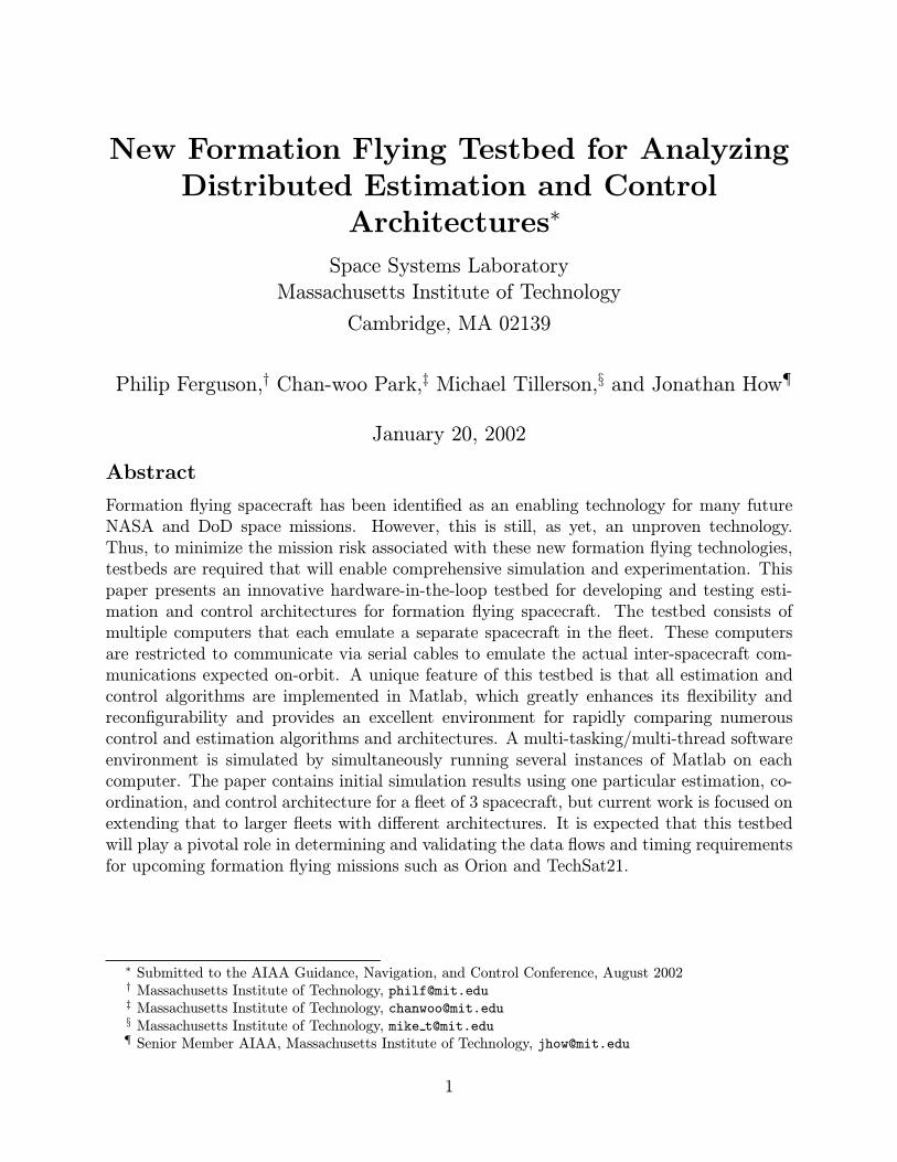
HIGH LEVEL COORDINATIONMultiple VehicleFormation Coordinator GNC Housekeeping

HighData Rate

LowData Rate

X/LINK

ABS/REL NAV ESTIMATOR

N/L ORBIT PROP

ATTITUDE ESTIMATOR

N/L ATT. MODEL

THRUSTER MAPPER

TORQ. COIL MODEL

SAT/CDH

��������������������������������������������������������������������������������

���������������������������������������

������������������������������������������������������������������������������������

������������������������������������������

Measurement Update (Abs)

AUTONOMOUS FORMATION CONTROLAUTONOMOUS FORMATION CONTROL

Measurement Update (Rel)

State Estimate (Abs, Rel) Parametric

Model

On orbitDisturbanceModel

ControlUpdate

State Propagation(Abs, Rel)

State EstimateUpdate (Abs, Rel)

Desired & CurrentStates

ControlUpdate

Parameter& Model Update

FlightModeMeasurement

Update (Att)Att Estimate

Control& ModelUpdate

LOW LEVEL SAT / CONTROLAttitude Control

RegulatorFuel/Time Optimal Planning

Attitude Propagation

Att. Estimate Update

Parameter& Model Update

Tcoil

Tthruster

uO/LuC/L

uFIRING

TFIRING

RawGPSData

Formation Coord.Mean Elm. Update Operations &

Flight Update

Figure 1: Interactions between the autonomous formation flying control algorithms.

position, velocity, attitude and fuel remaining on each spacecraft in the fleet, the data set

also contains information regarding the “distribution performance” which consists of a time

history of the events that occurred on each spacecraft as well as the amount of data that

was communicated. This data (computational load distribution, communication demands,

control performance) can then be used evaluate the trade-offs between the various estimation

and control architectures.

2 Architectures

Figure 1 shows the basic elements and information flow for a typical formation flying control

system [32]. The figure is intentionally complex in an attempt to show the complicated

information flow between the various estimation, coordination, and control algorithms. Some

of these algorithms can naturally be decentralized or distributed, but others require combined

information and thus must be performed within a centralized or hierarchic architecture.

However, to simplify the figure slightly, it is left as implicit that the estimation, coordination,

control algorithms could actually be distributed across the vehicles in the fleet.

Typically, the decision to be made with regards to architecture design is one of distribution.

Splitting up estimation, coordination, or control algorithms for distribution across the fleet

can provide benefits such as robustness, flexibility, speed, and improved autonomy. Fur-

thermore, the modularity inherent in distributed architectures usually lends itself easily to

expansion. Also, splitting up the algorithms for execution across the fleet allows for par-

4

allel processing which, if scaled properly, could dramatically reduce the computation time

compared to a completely centralized architecture. Of course, these benefits of distributed

architectures must be weighed against the apparent disadvantages, which include increased

inter-spacecraft communications, possible non-determinacy of solutions and higher mission

risk stemming from the increase in overall architecture complexity. When analyzing the

degree to which algorithms can be distributed, it is convenient to identify the following

categories:

• Centralized architectures — involve only one entity performing the primary computation

for the fleet using data collected at remote sites.

• Distributed architectures — wherein large parts of the computation are allocated to

other computational nodes in the fleet for parallel processing. Once each node has

completed its own computation, the result is passed back to a central location for

integration into the full solution. These architectures are characterized by the fact

that typically, the intermediate results found at each node before integration are not

meaningful on their own; they must be combined at a central location.

• Decentralized architectures — are similar to distributed architectures in that the overall

algorithm is executed in parallel across the fleet. However, in the case of distributed

architectures, the results that each individual node arrives at are meaningful and often

represent the desired computational solution. In this case, the final solution ends up

distributed across the entire fleet.

• Hierarchic architectures — involve hybrids of the above three architectures. Large fleets

of spacecraft can be split up into smaller clusters of spacecraft that each have their

own architecture.

The distinction between the different types of architectures is of paramount importance when

attempting to integrate several algorithms together. For instance, decentralized architectures

might appear superior as a stand-alone algorithm due to its highly parallel nature. However,

if the final result needs to be used in another algorithm that cannot be effectively distributed,

decentralized architectures could lose some of their advantage because the solution ends up

distributed across the entire fleet.

These architectures all involved distributed computation and significant communication of

both raw data (e.g. GPS carrier phase measurements) and solutions (estimated positions

and velocities, coordination solutions). As such, a sophisticated testbed is required that

can accurately assess the feasibility/performance of the proposed estimation and control

algorithms with correct computational and communication limitations in place.

5

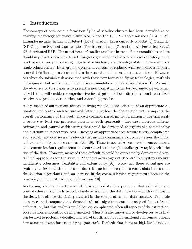
Figure 2: Orion Software Functional Block Diagram

3 Algorithms

One complication when analyzing various information architectures is that estimation, co-

ordination, and control algorithms must be developed for each configuration to correctly

establish the computation and communication requirements. In particular, in order to be

able to make specific statements regarding the benefits and/or disadvantages of certain ar-

chitectures, it is necessary to perform an in-depth analysis of several estimation and control

approaches. Fortunately, much work has been done on the navigation and control for for-

mation flying, and these techniques can be used in our analysis. This section presents

centralized and decentralized versions of an estimator using NAVSTAR GPS signals for nav-

igation, coupled with a fuel optimized decentralized/centralized coordination approach using

linear programming.

The algorithms presented here are part of a larger system that is currently being developed

for the Orion formation flying mission [13, 14]. A functional block diagram of the Orion

software system can be found in Figure 2. Some subsystems must interact with others in the

fleet while others are spacecraft specific. The basic components of the system are as follows:

• Orion Sequencer/Dispatcher: This software subsystem is responsible for sequencing

the events on the Orion spacecraft, including deciding when to run experiments. It

6

also directs all other subsystems over the course of a formation flying experiment. This

is both a vehicle-level and fleet-level problem.

• Navigation: Uses 6 GPS antennas with 3 dual RF front-end receivers to determine

relative and absolute position and velocity as well as spacecraft attitude using Carrier

Phase Differential GPS (CDGPS). This is both a vehicle-level and fleet-level problem.

• Planning/Coordination Control: Responsible for generating and executing fuel optimal

plans for fleet station-keeping and formation-change coordination. This is explicitly a

fleet-level problem.

• Attitude Control System: Controls the spacecraft attitude to enable adequate GPS

satellite visibility and ground communications. This is primarily a vehicle-level prob-

lem.

• Thruster Mapping: Oversees the thrust commands sent to the cold-gas thrusters on

the spacecraft. It feeds back the actual response given the requested ∆V and uses that

data to estimate the actual performance of the thrusters on orbit. This is explicitly a

vehicle-level problem.

• Serial Communication: Controls all serial communication (GPS receivers ⇔ science

computer, and CDH⇔ science computer, which is the path for data from other space-

craft in the fleet). This is primarily a vehicle-level problem.

Currently, only the State Sensing, Coordination Planner and a portion of the Sequencer and

Serial Communication subsystems have been implemented. Current work is focused on im-

plementing the other components of the control software. The following outlines some of the

algorithms currently used in the testbed. These include both centralized and decentralized

versions of the estimation and fleet coordination.

3.1 Estimation Algorithms

For the formation flying applications of interest in this paper, estimation of relative position

and velocity is performed using measurements from the NAVSTAR satellites. Attaching the

formation frame1 to a master vehicle (designated as vehicle m), the measurements from the

NAVSTAR constellation can then be written in vector form [15, 16] as

∆φsmi = Gm

"Xiτi

#+ βsmi + νsmi (1)

where

∆φsmi= differential carrier phase between vehicles m and i using

the NAVSTAR signals

1A local coordinate frame in which the relative states are defined.

7

Gi =

los1i 1

los2i 1...

...

losni 1

Xi = position of vehicle i relative to vehicle m

τi = relative clock bias between receivers on vehicles m and i

βsmi = carrier-phase biases for the single-differences

νsmi = carrier-phase noise of the NAVSTAR signals

Gi is the traditional geometry matrix. The components loski are the line-of-sights from the

ith user vehicle to the kth NAVSTAR satellite in the formation coordinate frame. For an

N -vehicle formation, these measurements are combined into one equation

∆Φs =

Gm 0

Gm. . .

0 Gm

X1τ1...

XN−1τN−1

+

βsm1βsm2...

βsmN−1

+ νs (2)

= GX + βs + νs (3)

where

∆Φs =

∆φsm1∆φsm2...

∆φsmN−1

and it is assumed that the master vehicle m has visibility to all available satellites and all

vehicles track the same set of satellites (See Ref. [23] for full details). This assumption is

consistent with the formation flying missions of interest that have relatively short baselines,

and thus all the vehicles can see the same set of NAVSTAR signals.

Doppler measurements using n NAVSTAR satellite signals can also be represented in vector

form. When differential Doppler measurements are formed between the master vehicle and

vehicle i,

∆φsmi = Gi

"Xiτi

#+ νsmi (4)

where

8

∆φsmi = differential carrier phase Doppler between vehicles m and i using the

NAVSTAR signals

Xi = velocity of vehicle i relative to vehicle m

τi = relative clock drift rate between receivers on vehicles m and i

νsmi = carrier-phase Doppler noise for the single-differences between vehicles

m and i using the NAVSTAR signals

For an N -vehicle formation, these measurements are combined into one equation

∆Φs =

G1 0

G2. . .

0 GN−1

X1τ1...

XN−1τN−1

+ νs (5)

= GvX + νs (6)

where

∆Φs =

∆φsm1∆φsm2...

∆φsmN−1

where it is also assumed that master vehicle m has visibility to all available satellites and all

of the vehicles track the same set of satellites.

These two velocity and position equations for formation vehicles can also be combined into

a single matrix equation"∆Φs

∆Φs

#=

"G 0

0 Gv

#"X

X

#+

"βs

0

#+

"νs

νs

#(7)

= H

"X

X

#+

"βs

0

#+

"νs

νs

#(8)

Decentralized/Centralized EKF: The following discusses the numerical, computational,

and implementation issues in the EKF state estimation problem for a fleet of vehicles. Note

that the formation of the differences indicated in Eqs. 1 and 4 explicitly requires that phase

information measured onboard two separate spacecraft be exchanged so that they can be

differenced. The estimation architecture selection must investigate various alternatives of

where/how to perform these differences. This analysis must include the cost to communi-

cate the basic phase/Doppler information, the computational effort to solve the estimation

9

problems (using extended Kalman filters — see Ref. [23] for full details), and the effort re-

quired to communicate the solutions to the computational nodes performing the coordination

and control calculations.

Note that, building on the work of [18, 20], Ref. [17] developed a different decentralized

approach for the spacecraft formation flying problem using a GPS sensor. However, the

work of [17] does not take full advantage of the decoupled observation structure in the

differential GPS sensing system. By taking this structure into account, this section presents

a simple and efficient decentralized approach to the formation estimation problem.

The sparse nature of the observation matrix H in Eq. 8 provides the basis for developing

the decentralized estimation algorithm, which reduces the processing time and yields better

numerical stability. In fact, the observation matrix H in Eq. 8 is completely block diagonal

if the master vehicle has visibility to all NAVSTAR satellites visible to the entire formation.

This would be the normal case for a closely spaced fleet of spacecraft in LEO, if the spacecraft

carry more than one antenna.2 In this case, Eq. 8 can be divided into N − 1 independent(and small) estimation filters (for N vehicles in the fleet) for each vehicle state relative to

the master vehicle. These estimation problems can then done in parallel by the master

vehicle or can easily be distributed amongst the vehicles in the formation. This simple,

straightforward distribution is possible because the relative dynamic models are also almost

completely decoupled.

This distribution of effort greatly reduces the computational load for the NAVSTAR-only

system, especially when the formation is quite large. As a result, the computational load per

vehicle in the decentralized system is significantly lower than that of the centralized system

and independent of the number of vehicles in the fleet. Note that, since the measurement

matrix decouples naturally, there is no degradation in the estimation performance as a result

of this decentralization.

The decentralized approach also provides a robust and flexible architecture that is less sen-

sitive to a single vehicle failure. For example, with a centralized solution approach, the

master vehicle performs most of the calculations for the fleet, therefore, unless all vehicles

are designed with the same processor as the master vehicle, the entire system could be sus-

ceptible to a single point failure. However, in the decentralized approach, all that is required

is that one spacecraft act as the reference vehicle which serves as the center of the formation

reference frame. The estimation process is then evenly distributed amongst the vehicles in

the fleet. As such, the vehicles could be designed to be identical in terms of their compu-

tational capability — and the CPU’s could be much simpler. Note that if one vehicle failed,

switching the reference vehicle from one spacecraft to another would be a much simpler

2Multiple antennas mounted on a spacecraft facing in different directions dramatically increase sky cov-erage [22, 21].

10

task than switching the master vehicle of the centralized approach. Furthermore, as shown

in Ref. [23], when compared to a centralized estimation scheme, the decentralized CDGPS

estimation process actually reduces the communication requirements between the vehicles.

3.2 Coordination Algorithms

With a large number of vehicles, the computational aspects of the fleet trajectory planning

are complicated by the large information flow and the amount of processing required. This

computational load can be balanced by distributing the effort over the fleet. For example, in

a typical formation flying scenario [25, 24], the vehicles will be arranged as part of a passive

aperture. These apertures provide relatively stable configurations that do not require as

much fuel to perform the science observations. But changing the viewing mode of the fleet

could require that the formation change configuration, moving from one aperture to another.

In this case it is essential to find fuel- and time-efficient ways to move each spacecraft to

their locations in the new aperture, which is a challenging optimization problem with many

possible final configurations.

The following describes a distributed solution to this problem (see [26] for details). The

approach partially alleviates the computational difficulties associated with solving the aper-

ture optimization problem by distributing the effort over the entire fleet, and then using a

coordinator to recombine the results. In this approach, the satellites analyze the possible

final locations in a discrete set of global configurations and associate a cost with each. The

linear programming tools that ship with Matlab are used to compute the fuel costs (and tra-

jectories) to move each spacecraft from their current location to each possible final location.

These simple calculations can be done in parallel by each spacecraft. The result is a list of

predicted fuel costs for every possible final location (called a ∆V map), which are used to

generate the fuel cost to move the fleet to each global configuration. These costs are based

on fuel usage, but they could include other factors, such as the vehicle health.

Note that, in the placement of the formation around the passive aperture, the only re-

quirement is that the vehicles be evenly spaced. Because the spacecraft are assumed to be

identical, their ordering around the aperture is not important, so this corresponds to an

assignment problem. In addition, the rotation of the entire formation around the aperture

is not important. Each rotation angle of the formation around the ellipse corresponds to

what is called a “global configuration.” To consider only a discrete set of configurations,

the aperture is typically discretized at 5◦ intervals. The ∆V maps are given to a centralizedcoordinator to perform the assignment process, which can be done in a number of ways.

To consider this assignment process in more detail, start by selecting one of the possible

locations on the closed-form aperture, and then the N − 1 equally spaced locations fromthat point. The N columns corresponding to these locations are then extracted from the

11

overall ∆V map to form the N ×N matrix

F =

f11 f12 · · · f1Nf21 f22 · · · f2N...

. . .

fN1 · · · · · · fNN

=hf1 f2 · · · fN

i(9)

the elements (fij) of which are the fuel cost for the ith satellite to relocate to the jth position.

The coordinator’s assignment problem can be solved using integer programming (IP) tech-

niques [30, 31, 27, 28]. Define the N ×N matrix Y , the elements yij of which are binary and

can be used to include logical conditions in the optimization. For example, yij = 1 would

correspond to the ith satellite being located at the jth position on the aperture (and yij = 0

if not).

Y =

y11 y12 · · · y1Ny21 y22 · · · y2N...

. . .

yN1 · · · · · · yNN

=hy1 y2 · · · yN

i(10)

With the vectors

F =hfT1 fT2 · · · fTN

i, Y =

y1...

yN

(11)

then the assignment problem for the coordinator can be written as

J?coord = minYF Y (12)

subject to

NXi=1

yij = 1 , ∀ j = 1, . . . , NNXj=1

yij = 1 , ∀ i = 1, . . . , N

yij ∈ {0, 1} ∀ i, j

(13)

Note that F Y calculates the fuel cost associated with each configuration, and the coordinator

selects the configuration that minimizes the total fuel cost for the fleet. The two summation

constraints ensure that each satellite is given a location and that only one vehicle is placed

at each location (an exclusive or condition) [30, 31, 27, 28]. The selection algorithm can be

modified to include the initial fuel conditions of each vehicle and to achieve fuel balancing

across the fleet [26].

With the discretization of the target aperture, this process is not guaranteed to be globally

12

optimal, but this hierarchical approach offers some key benefits in that it:

1. Distributes the computational effort of the reconfiguration optimization since most

calculations are done in parallel on much smaller-sized (LP and IP) problems.

2. Provides a simple method of finding optimized solutions that are consistent with the

global constraints since the centralized coordinator determines the final solution; and

3. Allows the vehicles to include individual decision models (e.g., bidding highly for a

maneuver that requires less re-orientation if there is a reaction wheel failure).

While the heuristic approach is faster to compute on this simple example, the advantage of

the integer optimization approach to the coordination is that it enables the trajectory design

and target aperture assignment to be combined into one centralized algorithm [27, 28].

This allows a centralized coordinator to explicitly include additional constraints, such as

collision avoidance and plume impingement, in the optimization. The technique has been

demonstrated on small fleets (e.g. N = 3), and further extensions are under investigation.

3.3 Formation-keeping Control

Disturbances such as differential drag, J2, and errors in the linearized dynamics will cause the

satellites to drift from the designed periodic motion associated with the passive apertures 3.

So control effort is required to maintain a state that results in the periodic motion. Linear

programming (LP) can be used to develop fuel-optimal control inputs to move the satellite

from the disturbed state back to the desired state, or to maintain the satellite within some

tolerance of the desired state.

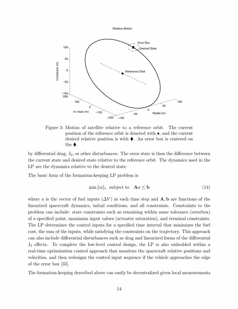
The formation-keeping problem is comprised of two issues. The first issue is what rela-

tive dynamics and initialization procedure should be used to specify the desired state to

maintain the passive aperture formation. The desired state is shown in Figure 3 as ¨ andthe reference orbit position as •. The periodic motion followed in the absence of distur-bances is also shown. The desired state can be determined from the closed form solutions

of the linearized dynamics and the initial conditions [29]. These initial conditions are then

used in the corresponding closed-form solutions to determine the desired state at any other

time. Reference [29] analyzes the use of various models to perform these initializations and

predictions.

The second issue for formation-keeping is which relative dynamics to use in the actual LP

problem. The error box is fixed to the desired state as in Fig. 3. The desired state is centered

in the error box, but the true state of the satellite will be disturbed from the desired state

3Typically short baseline periodic formation configurations that provide good, distributed, Earth imagingwhile reducing the tendency of the vehicles to drift apart.

13

−100−50

050

100

−200

−100

0

100

200−100

−50

0

50

100

Radial (m)

Desired State

Error Box

Reference Orbit

Relative Motion

In−track (m)

Cro

sstr

ack

(m)

Figure 3: Motion of satellite relative to a reference orbit. The currentposition of the reference orbit is denoted with •, and the currentdesired relative position is with ¨. An error box is centered onthe ¨.

by differential drag, J2, or other disturbances. The error state is then the difference between

the current state and desired state relative to the reference orbit. The dynamics used in the

LP are the dynamics relative to the desired state.

The basic form of the formation-keeping LP problem is

min kuk1 subject to Au ≤ b (14)

where u is the vector of fuel inputs (∆V ) at each time step and A,b are functions of the

linearized spacecraft dynamics, initial conditions, and all constraints. Constraints to the

problem can include: state constraints such as remaining within some tolerance (errorbox)

of a specified point, maximum input values (actuator saturation), and terminal constraints.

The LP determines the control inputs for a specified time interval that minimizes the fuel

cost, the sum of the inputs, while satisfying the constraints on the trajectory. This approach

can also include differential disturbances such as drag and linearized forms of the differential

J2 effects. To complete the low-level control design, the LP is also embedded within a

real-time optimization control approach that monitors the spacecraft relative positions and

velocities, and then redesigns the control input sequence if the vehicle approaches the edge

of the error box [33].

The formation-keeping described above can easily be decentralized given local measurements

14

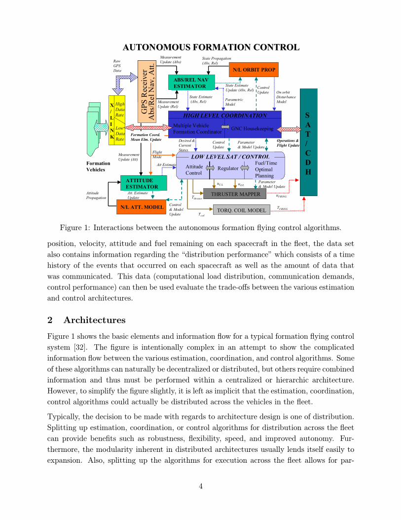
Figure 4: Physical Architecture of the Testbed

of the relative position/velocity of the satellite with respect to the desired state on the passive

aperture. However, this requires distributed knowledge of the desired states, which could, for

example, be obtained by propagating the states associated with a “template” of the desired

passive aperture [34, 35]. This template would be initialized using the GPS measurements

(absolute and relative) from all vehicles in the fleet. Thus formation-keeping algorithms will

involve a combination of centralized (template initialization, propagation, and monitoring)

and decentralized calculations (LP trajectory optimization).

4 Hardware-In-The-Loop Testbed

The testbed described in this paper can be used to simulate formation flying microsatellites

on-orbit from a computational and data flow perspective. The primary goal of the testbed

is to provide an environment wherein the distributed algorithms can easily be developed

and executed in scaled real-time over real communication links in a way that minimizes the

impact of the simulation on the actual algorithmic performance. The physical architecture

of the testbed is shown in Figure 4. The testbed is made up of four defining features:

Matlab: Matlab was chosen as the programming language for the testbed because of its ease

of algorithm implementation. Programming Matlab scripts does not require developers to

15

worry about complicated data management issues such as pointers and data casting. This is

because the primary focus of Matlab is algorithm development as opposed to computational

performance. Another benefit of using Matlab is that any Matlab toolboxes used in prelim-

inary algorithm development can continue to be used in the testbed. Having to re-write the

functions contained in these toolboxes significantly complicates the code development and

hinders the rapid architecture development desired for this testbed. This enables a seam-

less transition of new control and estimation approaches from various investigators to the

testbed. Working in matlab also provides a detailed window into the algorithms, which is

excellent for debugging. Of course, an additional hardware and OS specific analysis of the

software must be done prior to architecture acceptance to ensure it is within the capabilities

of the chosen computer.

A further benefit of Matlab is that it provides a very clean interface to Java, which is well-

known for its easy implementation of sockets and other external communications methods.

This Java extension permits low- and high-level data manipulation and transmission to be

carried out from within a Matlab function or script.

RS232 Serial Connectivity: A key aspect of the testbed is that, to retain as much realism

as possible, all inter-spacecraft communication is carried out through RS232 serial cables.

The RS232 serial protocol is very representative of inter-spacecraft communications modems

planned for most future microsatellite and Nanosat missions (e.g. [13, 14]). Through the use

of Java, the baud rate of the serial connections can be altered for simulation scaling. An

important aspect of inter-spacecraft communications of Nanosats is the method by which

multiple spacecraft can communicate with one another. Cost, power and mass typically

limit Nanosats to having very simple communications systems and thus require sophisticated

multiplexing algorithms to permit multiple spacecraft to use the same communications link.

In order to accurately model communication systems such as these, serial splitters have been

used to force each spacecraft to broadcast every outgoing message to each spacecraft in the

fleet. These are illustrated in Figure 4.

To facilitate 2-way communication amongst spacecraft, a “token bus” architecture is used

to ensure no data collisions occur on the “bus”, thus emulating a TDMA approach to inter-

spacecraft communications. Although TDMA was chosen as the original communications

architecture for the testbed, this can easily be changed to investigate other communications

scenarios such as FDMA or CDMA.

Multi-Threaded Applications: Many spacecraft software systems have several differ-

ent requirements that drive the need for multi-threaded applications. For example, large

optimization algorithms may take upwards of several minutes to compute. It would be im-

practical for all other spacecraft functions to have to wait for this optimization to complete

before addressing low-level tasks such as communications and state sensing. Thus, it is desir-

16

able to implement some tasks as “background” tasks while others occur in the “foreground”.

While Matlab does not have built-in support for multi-threaded applications, such programs

can be implemented on the testbed using several instances of Matlab on each computer.

Using this technique, the “Matlab Threads” communicate to each other on one spacecraft

through TCP/IP sockets. Socket communication provides a fast means of interprocess com-

munication with minimal impact to the rest of the system.

Simulation Engine: In addition to each PC representing a single spacecraft in the fleet,

there is one computer in the testbed that acts as the simulation engine. The purpose of

this computer is to propagate the states (position and attitude) of each spacecraft in the

fleet as well as the states of each GPS satellite for navigational purposes. At each time

step, the simulation computer transmits (via TCP/IP) the current simulation time as well

as simulated GPS signals that would be received by the spacecraft’s GPS antennas. The

data sent to each spacecraft computer from the simulation computer is an exact replica

of what would be received from the GPS receivers onboard each spacecraft. Using a GPS

simulator in the simulation engine forces each spacecraft to perform its own navigation

exactly as it would on-orbit. Since this data would be available virtually instantaneously

onboard each spacecraft, (independent of the inter-spacecraft data traffic) using TCP/IP as

the communications medium for this link alone (as well as for inter-process communication

as stated earlier) does not impact the architecture performance or analysis. Since TCP/IP is

an entirely separate data bus from the serial cables used for inter-spacecraft communications,

the simulation data in no way interferes with the inter-vehicle communications, thus retaining

representative data rates between spacecraft.

Utilizing a separate computer for simulation purposes increases the realism of the simulation

because it removes any code from the spacecraft computers that would not be run in the

actual flight system. Future versions of the testbed could even add a second computer to the

simulation engine for spacecraft visualization purposes. This computer would communicate

to the simulation propagator computer to receive the latest state vector of each spacecraft

and plot their relative positions in real-time.

5 Simulation Results

A preliminary simulation was run for this paper that implemented both the relative navi-

gation and reconfiguration algorithms in a distributed manner. The simulation involves 3

microsatellites on-orbit that are initially separated in-track, but are planning for a reconfig-

uration maneuver. In terms of Orion operational modes, this simulation covers “Compute

Mode” followed by “Active Control Mode”, as described in [14]. Although this presents a

point solution to the fleet estimation and control problem, it is necessary to analyze a par-

ticular solution in detail before statements can be made about distributed control in general.

This is because without real communication, computation and performance data, it is diffi-

17

cult to say anything concrete about the relative benefits of different architectures. Current

efforts are focused on extending these comparisons to other architectures.

For this simulation, both the estimation and planning are distributed across the entire fleet.

While the planning algorithm requires an initial estimate of the spacecraft state, the two

algorithms execute almost entirely independently. The basic computational flow of the al-

gorithms is as follows:

Estimation

1. Upon receipt of its raw GPS data, the master broadcasts the data to all slave spacecraft.

2. Each slave selects the appropriate matching time-tagged data set it has stored and

computes its relative state with respect to the master spacecraft.

Reconfiguration Coordination and Control

1. The master spacecraft decides to execute a reconfiguration maneuver and sends the

reconfiguration parameters to the slave spacecraft.

2. Each slave computes its fuel cost to each discretized position in the new configuration.

3. Each slave sends the fuel cost data to the master spacecraft.

4. The master spacecraft computes the optimal solution and broadcasts it to the slaves

along with a start time for the reconfiguration.

5. Each spacecraft computes its own trajectory corresponding to the optimal solution.

6. When the start time arrives, every spacecraft begins their plan.

Simulation

1. Each spacecraft computer sends its thruster inputs (if any) to the simulation via

TCP/IP.

2. The simulation engine propagates the position and attitude states of the fleet as well

as the GPS constellation.

3. GPS signals are simulated for the appropriate state and are broadcast to the spacecraft

computers via TCP/IP.

4. Steps 1 - 3 repeat every 5 seconds.

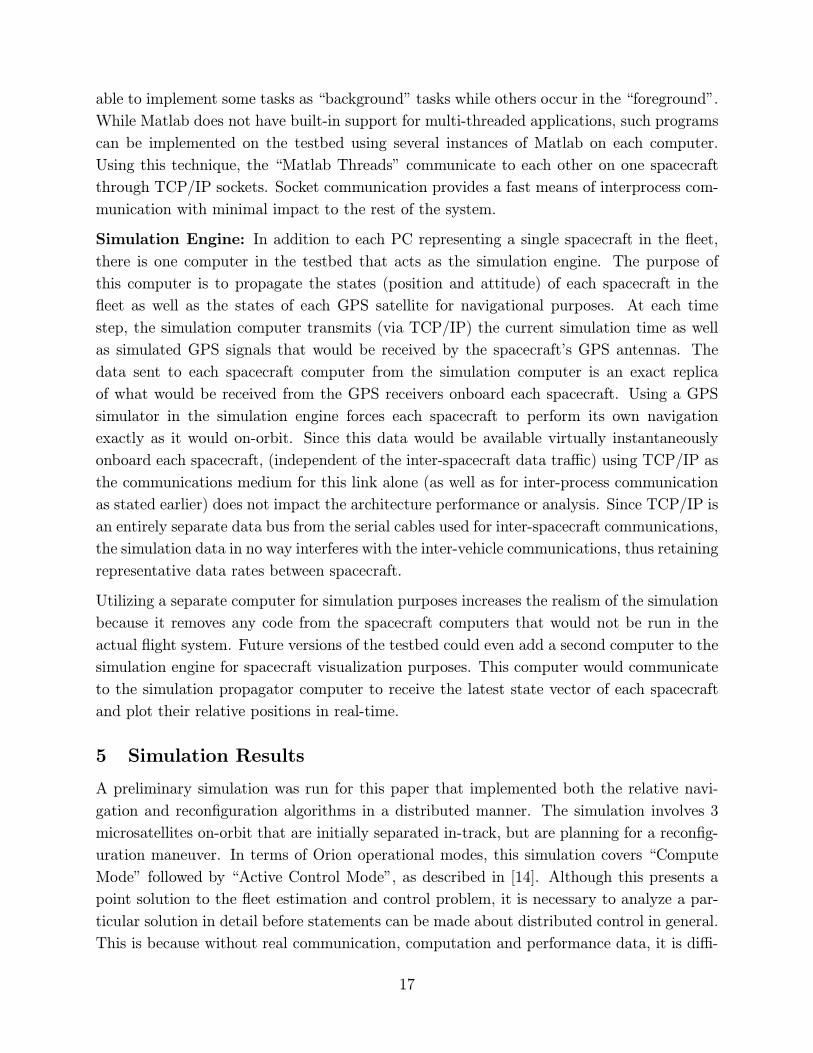
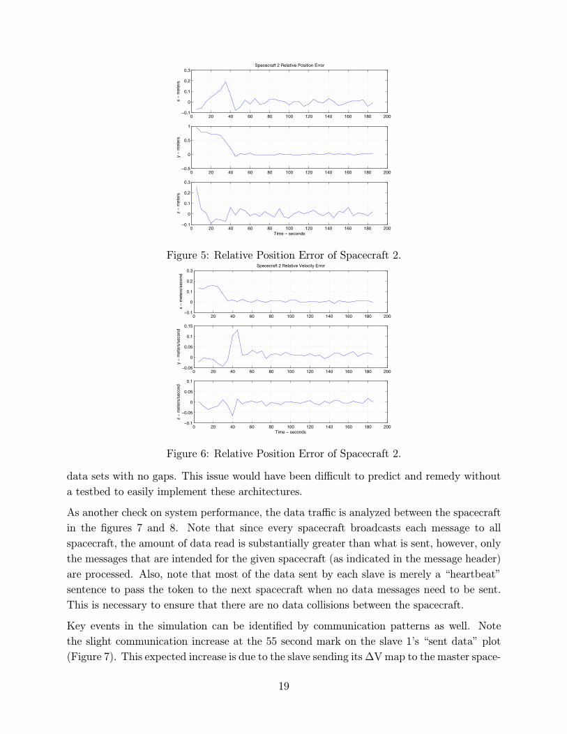
To analyze the performance of the relative navigation estimator, Figures 5 and 6 plot the

relative navigation error compared with the true state as propagated by the simulation

engine. This data indicates a brief settling period for the estimator followed by estimation

accuracies on the order of 2-5cm in position and 1cm/s in velocity. This indicates that the

basic distributed estimator is functioning correctly. The implementation of the decentralized

relative navigation software led to an interesting result that highlights the benefits of this

new testbed. Unstable estimation results indicated that a data synchronization problem was

occurring. A buffering system was needed as an addition to the estimator to ensure matching

18

0 20 40 60 80 100 120 140 160 180 200−0.1

0

0.1

0.2

0.3Spececraft 2 Relative Position Error

x −

met

ers

0 20 40 60 80 100 120 140 160 180 200−0.5

0

0.5

1

y −

met

ers

0 20 40 60 80 100 120 140 160 180 200−0.1

0

0.1

0.2

0.3z

− m

eter

s

Time − seconds

Figure 5: Relative Position Error of Spacecraft 2.

0 20 40 60 80 100 120 140 160 180 200−0.1

0

0.1

0.2

0.3Spececraft 2 Relative Velocity Error

x −

met

ers/

seco

nd

0 20 40 60 80 100 120 140 160 180 200−0.05

0

0.05

0.1

0.15

y −

met

ers/

seco

nd

0 20 40 60 80 100 120 140 160 180 200−0.1

−0.05

0

0.05

0.1

z −

met

ers/

seco

nd

Time − seconds

Figure 6: Relative Position Error of Spacecraft 2.

data sets with no gaps. This issue would have been difficult to predict and remedy without

a testbed to easily implement these architectures.

As another check on system performance, the data traffic is analyzed between the spacecraft

in the figures 7 and 8. Note that since every spacecraft broadcasts each message to all

spacecraft, the amount of data read is substantially greater than what is sent, however, only

the messages that are intended for the given spacecraft (as indicated in the message header)

are processed. Also, note that most of the data sent by each slave is merely a “heartbeat”

sentence to pass the token to the next spacecraft when no data messages need to be sent.

This is necessary to ensure that there are no data collisions between the spacecraft.

Key events in the simulation can be identified by communication patterns as well. Note

the slight communication increase at the 55 second mark on the slave 1’s “sent data” plot

(Figure 7). This expected increase is due to the slave sending its∆Vmap to the master space-

19

0 20 40 60 80 100 120 140 160 180 2000

2000

4000

6000Fleet Data Sent

Sen

t Dat

a −

Mas

ter(

byte

s)0 20 40 60 80 100 120 140 160 180 200

0

50

100

150

200

Sen

t Dat

a −

Sla

ve 1

(byt

es)

0 20 40 60 80 100 120 140 160 180 2000

50

100

150

200S

ent D

ata

− S

lave

2(b

ytes

)

Time − seconds

Figure 7: Data sent for each spacecraft.

0 20 40 60 80 100 120 140 160 180 2000

100

200

300Fleet Data Read

Rea

d D

ata

− M

aste

r(by

tes)

0 20 40 60 80 100 120 140 160 180 2000

1000

2000

3000

Rea

d D

ata

− S

lave

1(b

ytes

)

0 20 40 60 80 100 120 140 160 180 2000

1000

2000

3000

Rea

d D

ata

− S

lave

2(b

ytes

)

Time − seconds

Figure 8: Data read for each spacecraft.

craft for the final coordination optimization. In terms of computational flow performance,

the most illuminating performance metric to analyze is the types of data being transmitted

and received over time for a particular spacecraft. Transmitted data types indicate the types

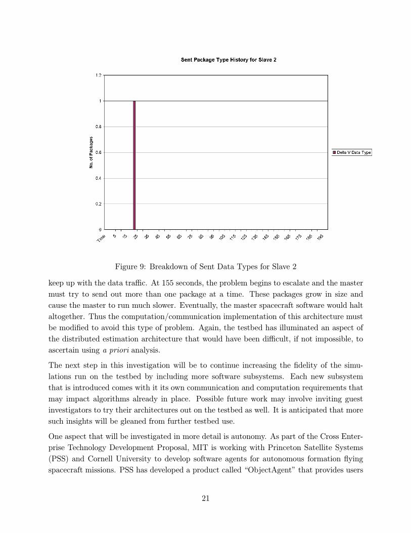
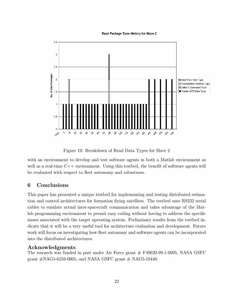
of events that are occurring across the fleet. Figures 9 and 10 illustrate the messages types

received by and sent from slave 2 in the fleet.

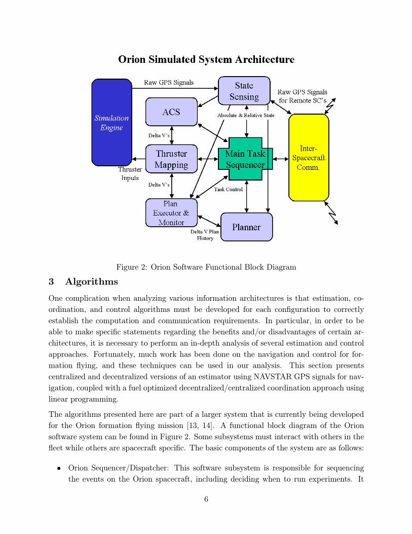
Figure 9 shows that the distribution of the algorithms has almost entirely eliminated the

need for the slaves to send data. The only message that is required is to send the ∆V map

to the master for optimization. This behavior was expected, however, some surprising issues

arise in the Figure 10, the read data history. Most of the data read is of the “Master GPS

Data Type”, which is the data package containing raw GPS measurements sent out by the

master every time-step. However, note that at 20 and 70 seconds, this package is not sent.

This indicates the master spacecraft is too bogged down with the current computations to

20

Figure 9: Breakdown of Sent Data Types for Slave 2

keep up with the data traffic. At 155 seconds, the problem begins to escalate and the master

must try to send out more than one package at a time. These packages grow in size and

cause the master to run much slower. Eventually, the master spacecraft software would halt

altogether. Thus the computation/communication implementation of this architecture must

be modified to avoid this type of problem. Again, the testbed has illuminated an aspect of

the distributed estimation architecture that would have been difficult, if not impossible, to

ascertain using a priori analysis.

The next step in this investigation will be to continue increasing the fidelity of the simu-

lations run on the testbed by including more software subsystems. Each new subsystem

that is introduced comes with it its own communication and computation requirements that

may impact algorithms already in place. Possible future work may involve inviting guest

investigators to try their architectures out on the testbed as well. It is anticipated that more

such insights will be gleaned from further testbed use.

One aspect that will be investigated in more detail is autonomy. As part of the Cross Enter-

prise Technology Development Proposal, MIT is working with Princeton Satellite Systems

(PSS) and Cornell University to develop software agents for autonomous formation flying

spacecraft missions. PSS has developed a product called “ObjectAgent” that provides users

21

Figure 10: Breakdown of Read Data Types for Slave 2

with an environment to develop and test software agents in both a Matlab environment as

well as a real-time C++ environment. Using this testbed, the benefit of software agents will

be evaluated with respect to fleet autonomy and robustness.

6 Conclusions

This paper has presented a unique testbed for implementing and testing distributed estima-

tion and control architectures for formation flying satellites. The testbed uses RS232 serial

cables to emulate actual inter-spacecraft communication and takes advantage of the Mat-

lab programming environment to permit easy coding without having to address the specific

issues associated with the target operating system. Preliminary results from the testbed in-

dicate that it will be a very useful tool for architecture evaluation and development. Future

work will focus on investigating how fleet autonomy and software agents can be incorporated

into the distributed architectures.

AcknowledgmentsThe research was funded in part under Air Force grant # F49620-99-1-0095, NASA GSFC

grant #NAG5-6233-0005, and NASA GSFC grant # NAG5-10440.

22

References

[1] F. H. Bauer, J. O. Bristow, J. R. Carpenter, J. L. Garrison, K. Hartman, T. Lee,

A. Long, D. Kelbel, V. Lu, J. P. How, F. Busse, P. Axelrad, and M. Moreau, “En-

abling Spacecraft Formation Flying through Spaceborne GPS and Enhanced Autonomy

Technologies,” in Space Technology, Vol. 20, No. 4, pp. 175—185, 2001.

[2] Enright, J., Sedwick, R., Miller, D., ”High Fidelity Simulation for Spacecraft Autonomy

Development”, Canadian Aeronautics and Space Journal, Dec. , 2001 (Forthcoming).

[3] F. H. Bauer, J. Bristow, D. Folta, K. Hartman, D. Quinn, J. P. How, “Satellite For-

mation Flying Using an Innovative Autonomous Control System (AUTOCON) Envi-

ronment,” proceedings of the AIAA/AAS Astrodynamics Specialists Conference, New

Orleans, LA, August 11-13, 1997, AIAA Paper 97-3821.

[4] F. H. Bauer, K. Hartman, E. G. Lightsey, “Spaceborne GPS: Current Status and Future

Visions,” proceedings of the ION-GPS Conference, Nashville, TN, Sept. 1998, pp. 1493—

1508.

[5] F. H. Bauer, K. Hartman, J. P. How, J. Bristow, D. Weidow, and F. Busse, “En-

abling Spacecraft Formation Flying through Spaceborne GPS and Enhanced Automa-

tion Technologies,” proceedings of the ION-GPS Conference, Nashville, TN, Sept. 1999,

pp. 369—384.

[6] Available at http://starlight.jpl.nasa.gov/.

[7] Available at http://nmp.jpl.nasa.gov/st5/.

[8] D. Miller et al. “SPHERES: A Testbed For Long Duration Satellite Formation Flying

In Micro-Gravity Conditions,” AAS00-110.

[9] T. Corazzini, A. Robertson, J. C. Adams, A. Hassibi, and J. P. How, “Experimental

demonstration of GPS as a relative sensor for formation flying spacecraft,” Fall issue of

the Journal of The Institute Of Navigation, Vol. 45, No. 3, 1998, pp. 195—208.

[10] E. Olsen, C.-W. Park, and J. How, “3D Formation Flight using Differential Carrier-

phase GPS Sensors,” The J. of The Institute Of Navigation, Spring, 1999, Vol. 146,

No. 1, pp. 35—48.

[11] F. D. Busse, How, J.P., Simpson, J., and Leitner, J., “PROJECT ORION-EMERALD:

Carrier Differential GPS Techniques and Simulation for Low Earth Orbit Formation

Flying,” Presented at IEEE Aerospace Conference, Big Sky, MT, Mar 10-17, 2001

[12] http://dshell.jpl.nasa.gov/

[13] J. How, R. Twiggs, D. Weidow, K. Hartman, and F. Bauer, “ORION: A low-cost

demonstration of formation flying in space using GPS,” AIAA/AAS Astrodynamics

Specialists Conference, Boston, MA, Aug. 1998.

23

[14] P. Ferguson, F. Busse, B. Engberg, J. How, M. Tillerson, N. Pohlman, A. Richards, R.

Twiggs, “Formation Flying Experiments on the Orion-Emerald Mission”, AIAA Space

2001 Conference and Exposition, Albuquerque, New Mexico, Aug. 2001, pp.

[15] E. Olsen, GPS Sensing for Formation Flying Vehicles. Ph.D. Dissertation, Stanford

University, Dept. of Aeronautics and Astronautics, Dec. 1999

[16] T. Corazzini, Onboard Pseudolite Augmentation for Spacecraft Formation Flying. Ph.D.

Dissertation, Stanford University, Dept. of Aeronautics and Astronautics, Aug. 2000

[17] J. R. Carpenter, D. C. Folta, D. A. Quinn NASA/Goddard Space Flight Center “

Integration of Decentralized Linear-Quadratic-Gaussian Control into GSFC’s Universal

3-D Autonomous Formation Flying Algorithm,” Proceedings of the AIAA Guidance

Navigation and Control Conference, Portland, OR, August 1999

[18] J. L. Speyer, “Computation and Transmission Requirements for a Decentralized Linear-

Quadratic-Gaussian Control Problem,” IEEE Trans. Automatic Control, vol. AC-24(2),

1979, pp.266-299.

[19] Schetter, T., Campbell, M., Surka, D., ”Comparison of Multiple Agent Based Organi-

zations for Satellite Constellations,” 2000 FLAIRS AI Conference, Orlando FL, April,

2000.

[20] A. G. O. Mutambara Decentralized Estimation and Control for Multisensor Systems,

CRC Press LLC, 1998

[21] J. C. Adams, Robust GPS Attitude Determination for Spacecraft. Ph.D. Dissertation,

Stanford University, Dept. of Aeronautics and Astronautics, 1999

[22] E. Glenn Lightsey, Development and Flight Demonstration of a GPS Receiver for Space.

Ph.D. Dissertation, Stanford University, Dept. of Aeronautics and Astronautics, Jan.

1997

[23] C. Park and J. P. How, “Precise Relative Navigation using Augmented CDGPS,” pro-

ceedings of the ION-GPS Conference, Sept. 2001

[24] Sedwick, R., Miller, D., Kong, E., “Mitigation of Differential Perturbations in Clusters

of Formation Flying Satellites,” Proceedings of the AAS/AIAA Space Flight Mechanics

Meeting, Breckenridge, CO, Feb. 7-10, 1999. Pt. 1 (A99-39751 10-12), San Diego, CA,

Univelt, Inc. (Advances in the Astronautical Sciences. Vol. 102, pt.1), 1999, p. 323-342.

[25] Das, A., Cobb, R., “TechSat 21 - Space Missions Using Collaborating Constellations

of Satellites,” Proceedings of AIAA/USU 12th Annual Conference on Small Satellites,

Utah State University, Logan, Aug. 31-Sept. 3, 1998, (A99-10826 01-20), Logan, UT,

Utah State University, 1998.

[26] M. Tillerson, G. Inalhan, and How, J. P.,“Coordination and Control of Distributed

Spacecraft Systems Using Convex Optimization Techniques,” accepted for publication

in the International Journal of Robust and Nonlinear Control, July 2001.

24

[27] T. Schouwenaars, B. DeMoor, E. Feron and J. How, “Mixed integer programming for

safe multi-vehicle cooperative path planning,” proceedings of the ECC, Sept 2001.

[28] Richards, A., Schouwenaars, T., How, J., Feron, E., “Spacecraft Trajectory Planning

With Collision and Plume Avoidance Using Mixed Integer Linear Programming,” pro-

ceedings of the AIAA Guidance, Navigation, and Control Conference, August 2001, and

submitted to the AIAA Journal of Guidance, Control and Dynamics, October, 2001.

[29] Tillerson, M. and How, J., “Advance Guidance Algorithms for Spacecraft Formation

Flying,” submitted to the 2002 American Control Conference, Sept 2001.

[30] C. A. Floudas, “Nonlinear and Mixed-Integer Programming — Fundamentals and Ap-

plications,” Oxford University Press, 1995.

[31] H. P. Williams and S. C. Brailsford, “Computational Logic and Integer Programming,”

in Advances in Linear and Integer Programming, Editor J. E. Beasley, Clarendon Press,

Oxford, 1996, pp. 249—281.

[32] G. Inalhan, F. D. Busse, and J. P. How. Precise formation flying control of multiple

spacecraft using carrier-phase differential GPS. AAS 00-109, 2000.

[33] M. Tillerson, G. Inalhan, and J. How, “Coordination and Control of Distributed Space-

craft Systems Using Convex Optimization Techniques,” submitted to the International

Journal of Robust and Nonlinear Control, Nov. 2000.

[34] R. Beard and F. Hadaegh, “Constellation templates: An approach to autonomous for-

mation flying”, in World Automation Congress, (Anchorage, Alaska), May 1998.

[35] J. Tierno “Collective Management of Satellite Clusters,” proceedings of the AFOSR

workshop on Dynamics and Control, August 2000.

25