Jerome F. Hajjar, Ph.D., P.E. Professor and Chair Department of Civil and Environmental Engineering Northeastern University Mark D. Denavit Department of Civil and Environmental Engineering University of Illinois at Urbana-Champaign Third International Symposium on Innovative Design of Steel Structures June 28 & 30, 2011 New Trends for Seismic Engineering of Steel and Composite Structures
Transcript
Jerome F. Hajjar, Ph.D., P.E.Professor and ChairDepartment of Civil and Environmental EngineeringNortheastern University
Mark D. DenavitDepartment of Civil and Environmental EngineeringUniversity of Illinois at Urbana-Champaign
Third International Symposium on Innovative Design of Steel StructuresJune 28 & 30, 2011
New Trends for Seismic Engineering of Steel and Composite Structures
OUTLINE
This image cannot currently be displayed.
Composite Steel/Concrete Systems
Articulated Fuse Self-Centering Systems
AISC Specification and Seismic Provisions
Available from http://www.aisc.org
Rewritten from scratch: 2005 AISC Specification for Structural Steel Buildings2010 AISC Seismic Provisions for Structural Steel Buildings
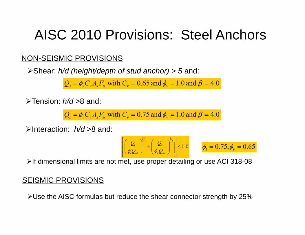
If dimensional limits are not met, use proper detailing or use ACI 318-08
AISC 2010 Provisions: Steel Anchors
New Organization in AISC 341‐10: Composite integrated into provisions
A. General RequirementsB. General Design RequirementsC. AnalysisD. General Member and Connection RequirementsE. Moment Frame SystemsF. Braced‐Frame and Shear‐Wall SystemsG. Composite Moment Frame SystemsH. Composite Braced‐Frame and Shear‐Wall SystemsI. Fabrication and ErectionJ. Quality Assurance and Quality ControlK. Prequalification and Cyclic Qualification Testing
• Composite Moment Frames• Composite Ordinary Moment Frames• Composite Intermediate Moment Frames• Composite Special Moment Frames• Composite Partially‐Restrained Moment Frames
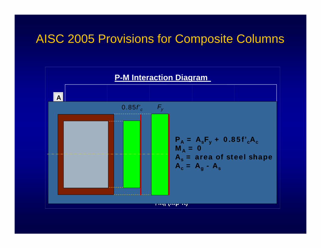
• Design recommendations:– Effective flexural (EIeff) and torsional rigidity (GJeff) for 3D analysis– Critical load (Pn) and column curves (Pn‐λ) for slender CFTs– P‐M interaction for slender CFTs– System behavior factors for composite systems (R, Cd, Ωo)– Direct analysis for composite systems
P/Po
AISCFiber Analysis
Mark D. DenavitUniversity of Illinois at Urbana‐Champaign
Urbana, Illinois
Jerome F. HajjarNortheastern UniversityBoston, Massachusetts
Tiziano PereaUniversidad Autónoma Metropolitana
Mexico DF, Mexico
Roberto T. LeonGeorgia Institute of Technology
Atlanta, Georgia
Sponsors: National Science FoundationAmerican Institute of Steel ConstructionGeorgia Institute of TechnologyUniversity of Illinois at Urbana‐Champaign
Non‐Seismic and Seismic Design of Composite Beam‐Columns and Composite Systems
Introduction
• Experimental assessment of limit surface– Slender CFT beam‐column tests
• Finite element formulation– Mixed beam‐column element– Steel and concrete uniaxial cyclic materials
– Localization and plastic hinge length
• Computational assessment of composite system behavior
Steel Girders
Composite Column
RCFTCCFT
MAST Lab
Specimens designed for
Closing databases gaps in: • L, λ, D/t, fc’
Maximize MAST capabilities:• Pz = 1320 kip• Ux=Uy=+/‐16”• 18’ < L < 26’• Other constraints
Specimen L Steel section Fy fc’ D/tname (ft) HSS D x t (ksi) (ksi)
• Schneider 1998• Johansson and Gylltoft 2002• Varma et al. 2002• Hu et al. 2003
• El‐Tawil and Deierlein 2001• Alemdar and White 2005• Tort and Hajjar 2007
Displacement
Force
Primary Unknown
Mixed
• Hajjar and Gourley 1997• Aval et al. 2002• Alemdar and White 2005
• de Souza 2000• El‐Tawil and Deierlein 2001• Alemdar and White 2005
• Nukala and White 2004• Alemdar and White 2005• Tort and Hajjar 2007
• Hajjar et al. 1998• Aval et al. 2002• Varma et al. 2002• Tort and Hajjar 2007
• Hajjar and Gourley 1997• El‐Tawil and Deierlein 2001• Inai et al. 2004
• Hajjar and Gourley 1997• El‐Tawil and Deierlein 2001
• Hajjar et al. 1998• Aval et al. 2002• Varma et al. 2002• Tort and Hajjar 2007
Mixed Beam‐Column Element• Mixed formulation with both
displacement and force shape functions
• Total‐Lagrangian corotational formulation
• Distributed plasticity fiber formulation: stress and strain modeled explicitly at each fiber of cross section
• Suitable for static and dynamic analysis
• Implemented in the OpenSeesframework
0 L
0
1Shape Functions
Tran
sver
seD
ispl
acem
ent
0 L0
1
Bend
ing
Mom
ent
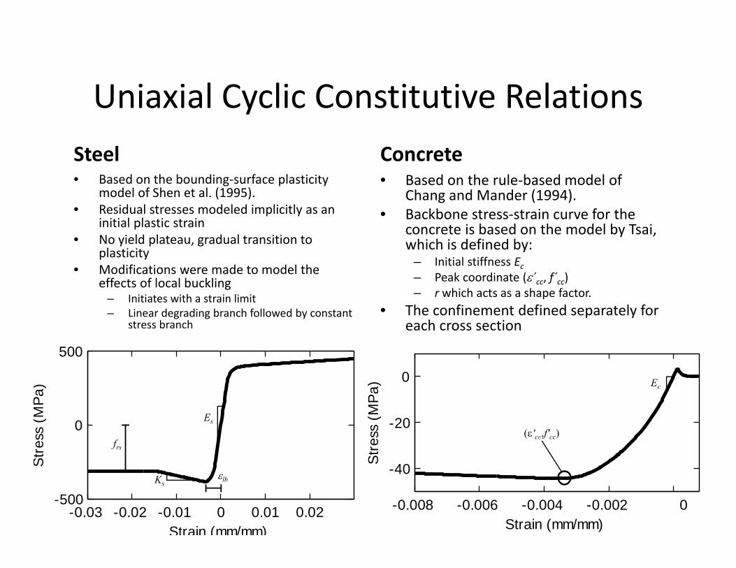
Uniaxial Cyclic Constitutive RelationsSteel• Based on the bounding‐surface plasticity
model of Shen et al. (1995).• Residual stresses modeled implicitly as an
initial plastic strain• No yield plateau, gradual transition to
plasticity• Modifications were made to model the
effects of local buckling– Initiates with a strain limit– Linear degrading branch followed by constant
stress branch
Concrete• Based on the rule‐based model of
Chang and Mander (1994). • Backbone stress‐strain curve for the
concrete is based on the model by Tsai, which is defined by:
– Initial stiffness Ec– Peak coordinate (ε´cc, f´cc)– r which acts as a shape factor.
• The confinement defined separately for each cross section
-0.008 -0.006 -0.004 -0.002 0
-40
-20
0
Strain (mm/mm)
Stre
ss (M
Pa)
(ε′cc,f′cc)
Ec
-0.03 -0.02 -0.01 0 0.01 0.02-500
0
500
Strain (mm/mm)
Stre
ss (M
Pa)
frs
Es
Ksεlb
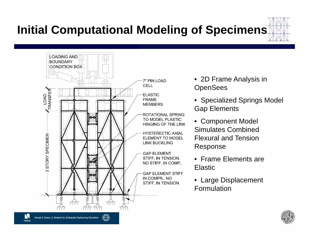
Validation of the Formulation
Specimen Name Reference Type D
(mm)t
(mm)f’c
(MPa)Fy
(Mpa)L
(mm)OtherDetails # of FE
CC4‐D‐4 Yoshioka et al. 1995 SC 450 2.96 40.5 283 1,350 NA 2scv2‐1 Han and Yao 2004 SC 200 3.00 58.5 304 300 NA 2CBC6 Elchalakani et al. 2001 BM 76.2 3.24 23.4 456 800 NA 1TBP005 Wheeler and Bridge 2004 BM 456 6.40 48.0 351 3,800 NA 4C4‐5 Matsui and Tusda 1996 PBC 165 4.50 31.9 414 661 e = 103 mm 4SC‐14 Kilpatrick and Rangan 1999 PBC 102 2.40 58.0 410 1,947 e = 40 mm 4
EC4‐D‐4‐06 Nishiyama et al. 2002 NBC 450 2.96 40.7 283 1,350 P = 4,488 kN 1EC8‐C‐4‐03 Nishiyama et al. 2002 NBC 222 6.47 40.7 834 666 P = 1,515 kN 1
F04I1 Elchalakani and Zhao 2008 CBM 110 1.25 23.1 430 800 NA 2F14I3 Elchalakani and Zhao 2008 CBM 89.3 2.52 23.1 378 800 NA 2
Comparison with Analysis
Specimen: 11C20‐26‐5CCFT 20x0.25
Fy = 44.3 ksi, f’c = 8.1 ksiL = 26 ft, KL = 52 ft
I-end J-end
u
uu
θ
θ
θ
θ
θ
θ
u
u uix
iy
iz jx
jy
jz
ixiy
iz
jxjy
jz
x
z
y
• Standard 3D 12 degree-of-freedom beam element• Effective elastic rigidities and updated Lagrangian geometric nonlinearity• Concentrated plasticity constitutive formulation
Finite Element Concentrated Plasticity “Macro” Model
• Behavior is modeled at member ends (at the centroidal axis) by:- Deformations (displacements and rotations)- Stress-resultants (forces and bending moments)
Element “degrees-of-freedom”
Macro Model Plasticity Formulation
Axial
Moment
Initial Bounding Surface
Final BoundingSurface
Initial LoadingSurface
Final LoadingSurface
{A }LS
{A }BS
{S}
{A} = Surface centroid{S} = Current location of force point
Force
{dS}
{dS} = Current location of force point
•Plastification is handled as a two step process:1. Isotropic hardening2. Kinematic hardening
Common assumption is that plasticity “yield” surfaces may change position and size but not shape
-10 -5 0 5 10-8
-6
-4
-2
0
2
4
6
8
10
X Displacement (in)
Y D
ispl
acem
ent (
in)
Tip Displacement
Load Case 4
-10 -5 0 5 10-8
-6
-4
-2
0
2
4
6
8
10
X Displacement (in)
Y D
ispl
acem
ent (
in)
Tip Displacement
Load Case 4Load Case 5
-10 -5 0 5 10-8
-6
-4
-2
0
2
4
6
8
10
X Displacement (in)
Y D
ispl
acem
ent (
in)
Tip Displacement
Load Case 4Load Case 5Load Case 6
-10 -5 0 5 10-8
-6
-4
-2
0
2
4
6
8
10
X Displacement (in)
Y D
ispl
acem
ent (
in)
Tip Displacement
Load Case 4Load Case 5Load Case 6Load Case 7
-10 -5 0 5 10-8
-6
-4
-2
0
2
4
6
8
10
X Displacement (in)
Y D
ispl
acem
ent (
in)
Tip Displacement
Load Case 4Load Case 5Load Case 6Load Case 7Load Case 8
-10 -5 0 5 10-8
-6
-4
-2
0
2
4
6
8
10
X Displacement (in)
Y D
ispl
acem
ent (
in)
Tip Displacement
Load Case 4Load Case 5Load Case 6Load Case 7Load Case 8Load Case 9
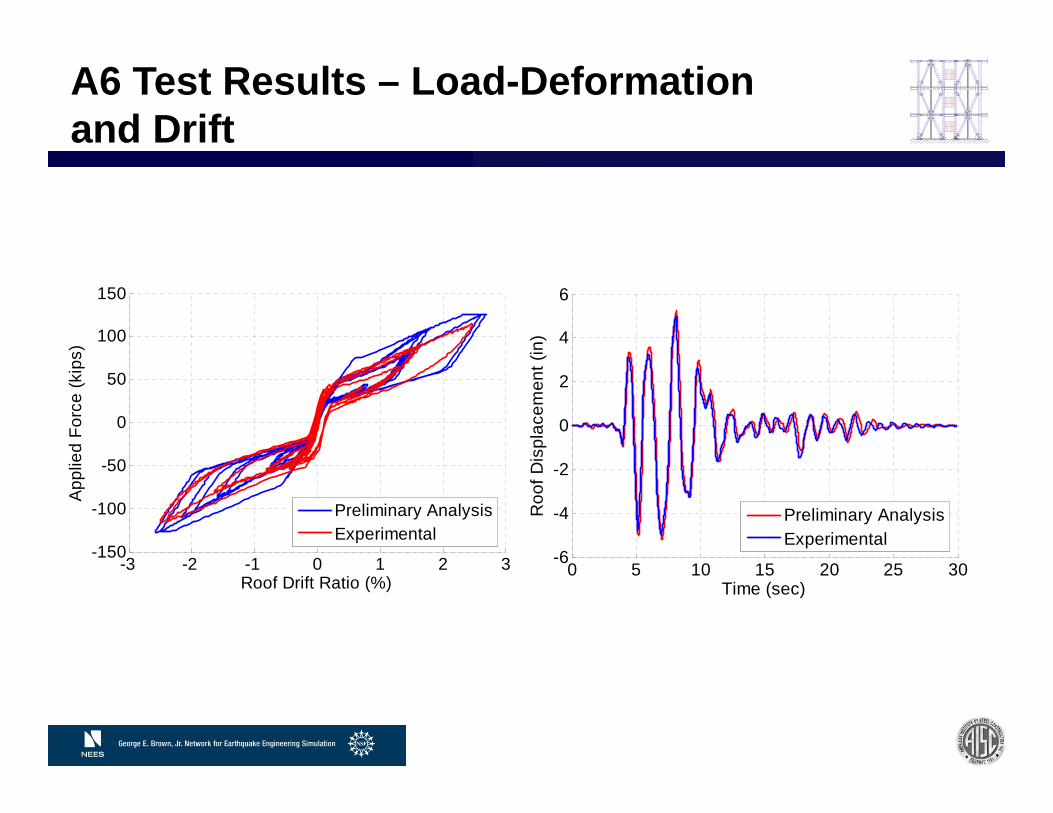
Tsuyoshi Hikino, Hyogo Earthquake Engineering Research Center, NIEDDavid Mar, Tipping & Mar Associates and Greg Luth, GPLA
In-Kind Funding: Tefft Bridge and Iron of Tefft, IN, MC Detailers of Merrillville, IN, Munster Steel Co. Inc. of Munster, IN, Infra-Metals of Marseilles, IN, and
Textron/Flexalloy Inc. Fastener Systems Division of Indianapolis, IN.
41
single frame dual frames
Develop a new structural building system that employs self-centering rocking action and replaceable fuses to provide safe and cost effective earthquake resistance.
-- minimize structural damage and risk of building closure
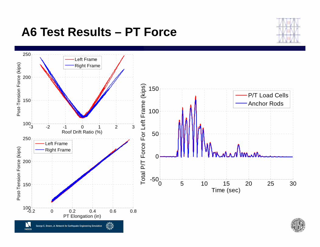
Controlled-Rocking System
• Corner of frame is allowed to uplift.
• Fuses absorb seismic energy
• Post-tensioning brings the structure back to center.
Result is a building where the structural damage is concentrated in replaceable fuses with little or no residual drift
Controlled-Rocking System
This image cannot currently be displayed.
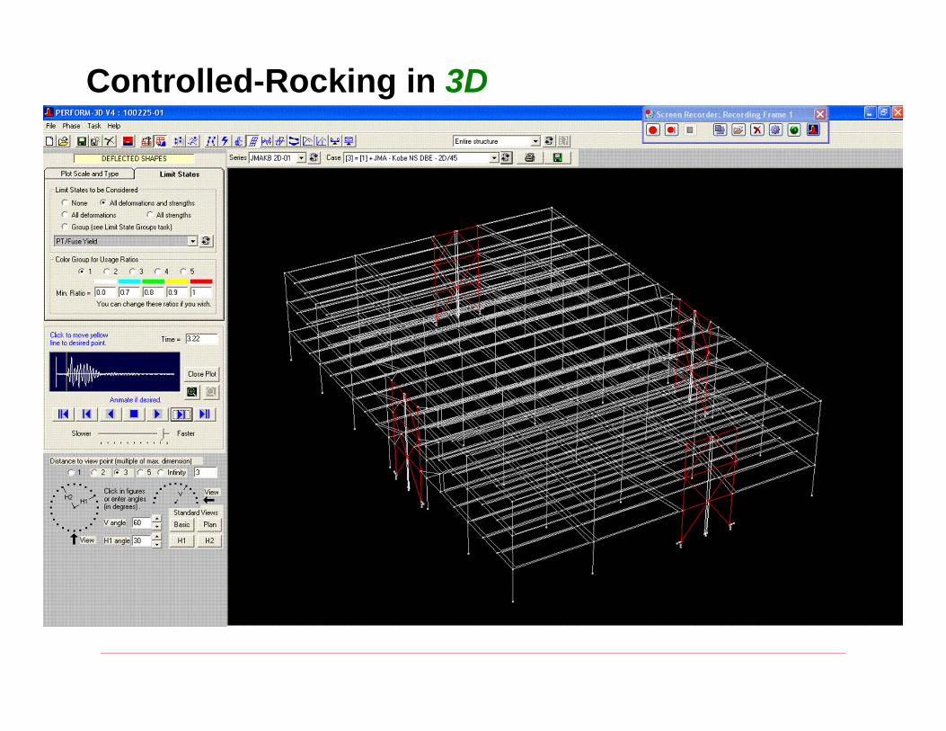
Controlled-Rocking in 3D
Bas
e Sh
ear
Drift
a
b c
d
f
g
Combined System
Origin-a – frame strain + small distortions in fusea – frame lift off, elongation of PTb – fuse yield (+)c – load reversal (PT yields if continued)d – zero force in fusee – fuse yield (-)f – frame contactf-g – frame relaxationg – strain energy left in frame and fuse, small residual displacement
Fuse System
Bas
e Sh
ear
Drifta
b c
d
efg
Fuse Strength Eff. FuseStiffness
PT Strength
PT – Fuse Strength
Pretension/Brace SystemB
ase
Shea
r
Drift
a,f bcde
g PT Strength
Frame Stiffness
e
2x FuseStrength
1. A/B ratio – geometry of frame
2. Overturning Ratio (OT) – ratio of resisting moment to design overturning moment. OT=1.0 corresponds to R=8.0, OT=1.5 means R=5.3
3. Self-Centering Ratio (SC) – ratio of restoring moment to restoring resistance.
4. Initial P/T stress
5. Frame Stiffness
6. Fuse type including degradation
)( BAVFA
MMSC
P
PT
resist
restore
+==
OVT
PPT
OVT
resist
MBAVFA
MMOT )( ++
==
Parametric Study of Prototype: Parameters Studied
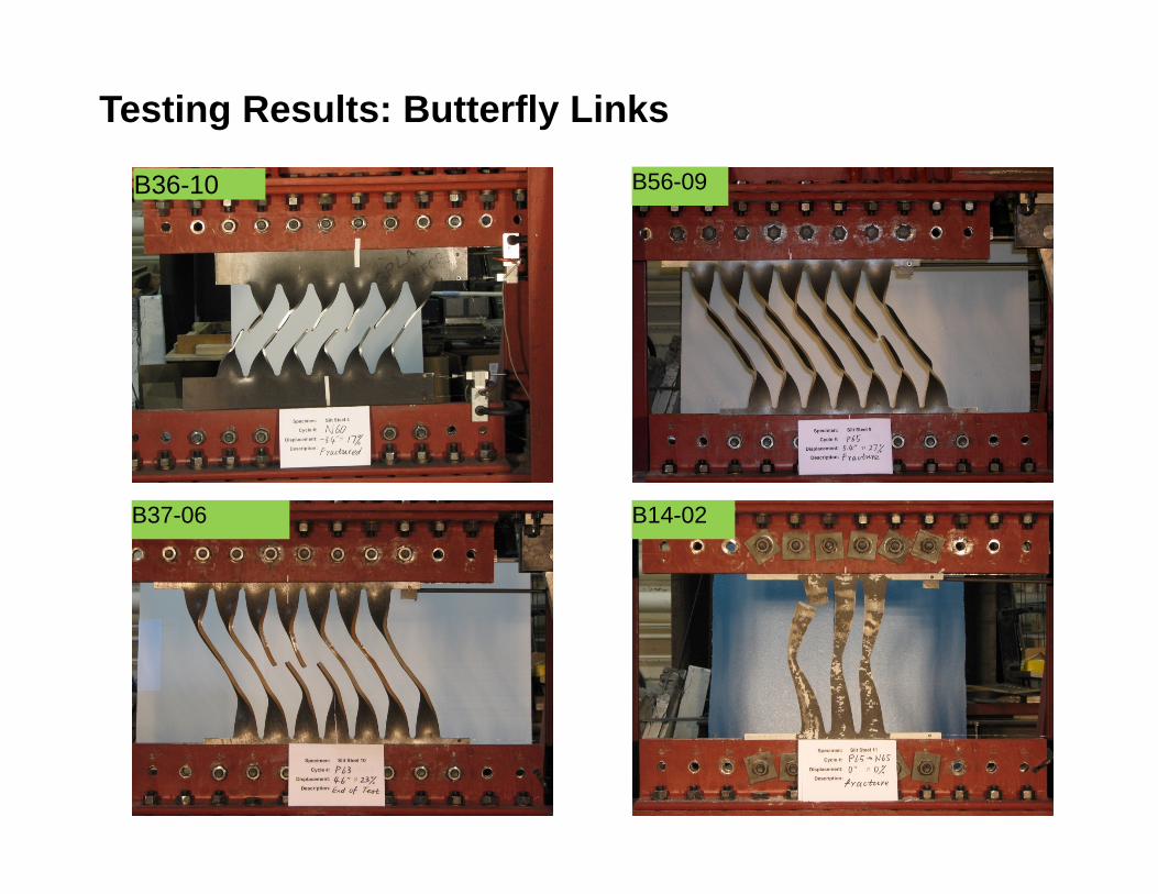
Shear Fuse Testing - Stanford
Panel Size: 400 x 900 mm
Attributes of Fuse- high initial stiffness- large strain capacity- energy dissipation