New Ultrasonic Techniques for Detecting and Quantifying ...

0

New Ultrasonic Techniques for Detecting andQuantifying Railway Wheel-Flats

Jose Brizuela1, Carlos Fritsch1 and Alberto Ibáñez2

1Consejo Superior de Investigaciones Científicas (CSIC)2Centro de Acústica Aplicada y Evaluación No Destructiva - CAEND (CSIC-UPM)

Spain

1. Introduction

The railway transport braking processes are likely to form surface defects on the tread if thewheel locks up and slides along the rail. This action can be produced by a defective, frozenor incorrectly tuned brake, as well as by a low rail-wheel adhesion caused by environmentalconditions (rain, snow, leaves, etc.). The abrasive effect of skidding causes a high wear on therolling surface (a wheel-flat), with lengths ranging typically from 20 to over 100 mm.

The rise in temperature caused by abrasion followed by a fast cooling may lead to theformation of brittle martensite beneath the wheel-flat. This can be associated to the beginningof further flaws like cracks and spalls with the loss of relatively large pieces of tread material.When the wheel rolls over a flat, high impact forces are developed and may cause a rapiddeterioration of both, rolling and fixed railway structures. Moreover, the incidence of hotbearings, broken wheels and rail fractures are coincidental with the number of wheel-flatsand out-of-round wheels (Kumagai et al., 1991; Snyder & Stone, 2003; Vyas & Gupta, 2006;Zakharov & Goryacheva, 2005).

Besides, when a critical speed is reached, a loss of rail-wheel contact occurs which produceshigh-levels of noise and vibrations that also affect passengers comfort. Finally in theworst-case scenario, surface defects on treads can cause a derailment (Wu & Thompson, 2002;Zerbst et al., 2005).

Therefore, there is a great interest in finding methods for an early detection and evaluationof surface defects without dismantling wheelsets due to their complex assembly (Pohl et al.,2004). Ideally, in order to reduce time and costs, inspection systems should be placed atthe end of train-wash stations or at the entrance of maintenance shops, where trains passfrequently at low speed.

Nowadays, many automatic and on-line wheel tread surface defect detection systems havealso been developed for the railway industry. Most of them can be classified into one of thefollowing categories:

Measurement of the impact forces in an instrumented rail: the Wheel Impact Load Detector(WILD) developed by Salient Systems, Inc. (2010) is the most popular system to detectwheel-flats; it consists of a large number of strain gauges mounted in the rail web, which

15

www.intechopen.com

2 Will-be-set-by-IN-TECH

are used to quantify the force applied to the rail through a mathematical relationshipbetween the applied load and the deflection of the foot of the rail. As a result, the wheelshealth and the safe train operations can be ensured by monitoring these impact forces(Stratman et al., 2007). In other cases, accelerometers are used instead (Belotti et al., 2006;Madejski, 2006). These techniques analyse the impacts produced by flats or other kind offlaws, but give no indications about their size.

Wheel radius variations measurement: in this case, the flange is considered perfectly roundand wear-free, being used as a reference to estimate the variations in the wheel radius.Mechanical (Feng et al., 2000; He et al., 2005) and optical (Gutauskas, 1992) systems havebeen designed based on this idea. Nevertheless, the hostile railway environment involvessome disadvantages for these methods, both are sensitive to vibrations and their resolutionis limited. Furthermore, small irregularities or adherences in the flange will lead to falseindications.

Ultrasonic flaw detection and measurement: the Non Destructive Testing (NDT) techniquesby ultrasound are often used for offline wheel examination; most of them require complexinstallations and/or machineries (Kappes et al., 2000). However, recent designs have beendeveloped for online wheel tread inspection using ultrasonic methods. Such systemsconsist in sending an ultrasound pulse over the rolling surface to detect echoes producedby cracks. The interrogating Rayleigh wave is generated by a transducer (EMAT orpiezoelectric) which is fired when the wheel passes over it; the same or other sensor canreceive reflections originated on flaws (Fan & Jia, 2008; Ibáñez et al., 2005; Salzburger et al.,2008). Unfortunately, wheel-flats usually have smooth edges that do not generate echoes,so it is very difficult to detect them by these techniques. Moreover, acoustic couplingbetween transducers and wheels frequently give rise to unreliable measurements due tovariability problems.

The aim of this chapter is to present an innovative ultrasound technique designed to detectand quantify wheel-flats that have been formed on the railway wheel tread. An extendedtheoretical framework supports the proposed method. It can be applied to trains movingat low speed (10-15 Km/h typical) and allows all the wheelsets mounted in a train to beinspected within a few seconds.

2. Alternative methodology

The proposed method differs from other conventional ultrasonic flaw detection approaches,which are based on the reflectivity of static flaws. In this case, surface waves are sent overa measuring rail instead of the rolling surface to interrogate the rail-wheel contact pointposition. Wheel-flats are then detected and sized by analysing the kinematic of the wheel-railcontact point echo.

The proposed technique comes up with many other advantages for railway industry, e.g., nomoving parts are involved in the measuring system; the set of transducer and measuring-railis invariant, so it can be fully characterized once; results are independent of wheel weardegree, no exploring pulses along rolling surface are sent; finally, an optimum ultrasoniccoupling between transducer and rail can be achieved.

Following this methodology two alternatives have been considered to determine wheel-flats:the first one is based on Doppler techniques which are suitable to detect velocity changes of amoving reflector (in this case the rail-wheel contact point). The second consist in measuring

400 Reliability and Safety in Railway

www.intechopen.com

New Ultrasonic Techniques for Detecting and Quantifying Railway Wheel-Flats 3

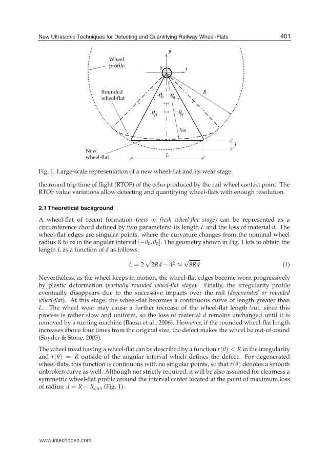
Fig. 1. Large-scale representation of a new wheel-flat and its wear stage.

the round trip time of flight (RTOF) of the echo produced by the rail-wheel contact point. TheRTOF value variations allow detecting and quantifying wheel-flats with enough resolution.

2.1 Theoretical background

A wheel-flat of recent formation (new or fresh wheel-flat stage) can be represented as acircumference chord defined by two parameters: its length L and the loss of material d. Thewheel-flat edges are singular points, where the curvature changes from the nominal wheelradius R to ∞ in the angular interval [−θ0, θ0]. The geometry shown in Fig. 1 lets to obtain thelength L as a function of d as follows:

L = 2√

2Rd − d2 ≈√

8Rd (1)

Nevertheless, as the wheel keeps in motion, the wheel-flat edges become worn progressivelyby plastic deformation (partially rounded wheel-flat stage). Finally, the irregularity profileeventually disappears due to the successive impacts over the rail (degenerated or roundedwheel-flat). At this stage, the wheel-flat becomes a continuous curve of length greater thanL. The wheel wear may cause a further increase of the wheel-flat length but, since thisprocess is rather slow and uniform, so the loss of material d remains unchanged until it isremoved by a turning machine (Baeza et al., 2006). However, if the rounded wheel-flat lengthincreases above four times from the original size, the defect makes the wheel be out-of-round(Snyder & Stone, 2003).

The wheel tread having a wheel-flat can be described by a function r(θ) < R in the irregularityand r(θ) = R outside of the angular interval which defines the defect. For degeneratedwheel-flats, this function is continuous with no singular points, so that r(θ) denotes a smoothunbroken curve as well. Although not strictly required, it will be also assumed for clearness asymmetric wheel-flat profile around the interval center located at the point of maximum lossof radius: d = R − Rmin (Fig. 1).

401New Ultrasonic Techniques for Detecting and Quantifying Railway Wheel-Flats

www.intechopen.com


Fig. 2. Scheme used to determine the wheel-flat loss of material d. The wheel moves towards+ x direction on the reference system (1). Pay attention that ϕ < 0 and the displacements < 0. It is assumed that effects such as creep, spin, and slip, are ignored, so the contact is notlost in the time domain. The contact point Q is defined in system (2) by its polar coordinates(r(θ), θ) = (r(γ − ϕ), γ − ϕ), while in (3) they are (q(γ, ϕ), γ). The rotation angle ϕ at eachinstant represents the difference between fixed and mobile systems, both mounted on thewheel center.

2.1.1 Rail-wheel contact point kinematic

The wheel rotation around its contact point Q can be described by following the scheme inFig. 2, where can be find three reference systems:

1) A coordinate system fixed on the measuring rail.

2) A system linked to the wheel shaft and parallel to the system 1.

3) A coordinate system attached to the wheel center in motion with vector �Q.

Note that, the rail is always tangent to the wheel at the contact point. When the wheel rollsover a perfectly rounded region the wheel center projection P on the rail coincides with thewheel-rail contact point Q (that means P = Q) since, in a circunference, radius and unitarytangent vector (�t) at Q are perpendicular. However, when the wheel rolls over its non circular

region [−θH , θH ] it rotates an angle ϕ, so vectors �Q and�t are not orthogonal. Moreover, thecontact point and the projection are moved apart in a distance s which is a function of ϕ,reflecting an advance or delay of Q in relation to P. In other words:

a) when −θH < ϕ ≤ 0, P leads Q and s ≤ 0;

b) for 0 < ϕ < θH , P lags Q and s > 0.

Fig. 2 shows the situation when ϕ < 0, so the contact point is behind the wheel centerprojection. On the other hand, each point of the wheel tread is described by�r(θ) = (r(θ), θ)on reference system 2, while on system 3 the coordinates are: (r(θ), θ) = (q(γ, ϕ), γ). Then,the transition from one system to another is given by:

q(γ, ϕ) = r(γ − ϕ) (2)


www.intechopen.com


and∂ (q(γ, ϕ))

∂γ=

∂ (r(γ − ϕ))

∂γ= r(γ − ϕ) (3)

Assuming that contact is not lost while the wheel is moving and the train speed ν is constantover the measuring rail. So, the rail-wheel contact point is defined for each rotated angle ϕ asQ =

(

q(γQ, ϕ), γQ

)

, such that its ordinate value q(γ, ϕ) sin(γ) is minimal on γQ, that is:

∂ (q(γ, ϕ) sin(γ))

∂γ

∣

∣

∣

∣

∣

γ=γQ

=∂ (q(γ, ϕ))

∂γ

∣

∣

∣

∣

∣

γ=γQ

sin (γQ) + q(γQ, ϕ) cos (γQ) = 0 (4)

Replacing eqs. (2) and (3) on (4), it is possible to figure out the tangent value at Q, which is:

tan (γQ) = − r(

γQ − ϕ)

r(

γQ − ϕ) (5)

The contact point Q belongs to the instantaneous axis of rotation, which remains steady foreach ϕ value, and the wheel center movement can be described, at all time, as a pure rotationaround Q. Additionally, as the angular velocity ω is an invariant and independent of anyreference systems used, the velocity vector is defined by:

�ν = −�ω × �Q = −�ω ×�r(

γQ − ϕ)

(6)

where

�ω = ω�k (7)

�r(

γQ − ϕ)

=(

q(γQ, ϕ) sin (γQ))

�j +(

q(γQ, ϕ) cos (γQ))

�i (8)

Solving the cross product (6), it yields to:

�ν =

∣

∣

∣

∣

∣

∣

�i �j �k0 0 ω

q(γQ, ϕ) cos γQ q(γQ, ϕ) sin γQ 0

∣

∣

∣

∣

∣

∣

= ωq(γQ, ϕ) sin (γQ)�i−ωq(γQ, ϕ) cos (γQ)�j (9)

As a result, there are two velocity components on (9). The first on�i-direction, means the trainspeed. By taking into account (2):

ν = ω q(γQ, ϕ) sin (γQ) = ω r(

γQ − ϕ)

sin (γQ) (10)

On the other hand, regarding eqs. (5) and (10), the velocity component in the�j-direction is:

�νy = −ω q(γQ, ϕ) cos (γQ) = ω r(

γQ − ϕ)

sin (γQ) = − ν

tan (γQ)(11)

As (11) expresses, for a perfect rounded wheel, the contact point Q will be located at 3π/2,so �νy will be null. Note as well on Fig. 2, that the displacement distance between the contactpoint Q and the wheel center projection P denoted by s(ϕ) is the x-coordinate on the referencesystem 2. That is:

s(ϕ) = −r(

γQ − ϕ)

cos (γQ) = −q(γ, ϕ) cos (γQ) (12)


www.intechopen.com


Fig. 3. Position of points P and Q on the reference system fixed to the rail, when the wheelpasses over an irregularity.

Therefore, the wheel center vertical movement can be related with the displacement s(ϕ) byreplacing (12) on (11):

�νy = ω s(ϕ) (13)

Thus, the wheel center vertical movement is zero for perfectly rounded wheels. However overa wheel-flat irregularity, the wheel center goes down a distance equal to the maximum loss ofmaterial d. Afterwards, it starts to rise again up to reach the radius nominal value just whenthe contact point comes out of the irregularity. As a result, the total wheel center displacementis 2d from the time instant t1 to t2, when the wheel rolls over the irregularity:

2d =∫ t2

t1

∣

∣νy

∣

∣dt =∫ t2

t1

|ω s(ϕ)|dt =∫ ϕH

−ϕH

|s(ϕ)|dϕ (14)

where the limits of integration −ϕH and ϕH correspond to the angular range that determinesthe irregularity. Hence, (14) gives the parameter d as a function of displacements s(ϕ) whichcan be measured; then the original wheel-flat length is obtained by (1). On the other hand, ass(ϕ) is a continuous function even if singular points are present, (14) is valid for any kind ofwheel-flats (new, partially rounded or degenerated). This property can be generalized as:

“For small irregularities, whatever is the wheel-flat wear degree from the original one, the area below|s(ϕ)| is two times the loss of material d”.

As well, since s(ϕ) = 0 in the round part of the wheel (|ϕ| > ϕH), the limits of integration maybe extended to any angle ϕA ≥ ϕ for single or isolated wheel-flats cases. Using an auxiliaryparameter α in order to cover a full wheel revolution (14) can be written as:

d(α) =∫ α+ϕA

αs(ϕ) dϕ where 0 ≤ α ≤ 2π − ϕA and ϕA ≥ ϕ (15)

2.1.2 Rail-wheel contact point velocity

When the wheel moves over the rail the instantaneous position of the wheel center projectionis given by x, while the contact point Q is x + s. Note that the distance x is now measured


www.intechopen.com


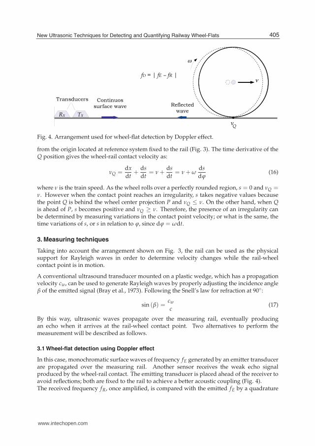
Fig. 4. Arrangement used for wheel-flat detection by Doppler effect.

from the origin located at reference system fixed to the rail (Fig. 3). The time derivative of theQ position gives the wheel-rail contact velocity as:

νQ =dx

dt+

ds

dt= ν +

ds

dt= ν + ω

ds

dϕ(16)

where ν is the train speed. As the wheel rolls over a perfectly rounded region, s = 0 and νQ =ν. However when the contact point reaches an irregularity, s takes negative values becausethe point Q is behind the wheel center projection P and νQ ≤ ν. On the other hand, when Qis ahead of P, s becomes positive and νQ ≥ ν. Therefore, the presence of an irregularity canbe determined by measuring variations in the contact point velocity; or what is the same, thetime variations of s, or s in relation to ϕ, since dϕ = ωdt.

3. Measuring techniques

Taking into account the arrangement shown on Fig. 3, the rail can be used as the physicalsupport for Rayleigh waves in order to determine velocity changes while the rail-wheelcontact point is in motion.

A conventional ultrasound transducer mounted on a plastic wedge, which has a propagationvelocity cw, can be used to generate Rayleigh waves by properly adjusting the incidence angleβ of the emitted signal (Bray et al., 1973). Following the Snell’s law for refraction at 90◦:

sin (β) =cw

c(17)

By this way, ultrasonic waves propagate over the measuring rail, eventually producingan echo when it arrives at the rail-wheel contact point. Two alternatives to perform themeasurement will be described as follows.

3.1 Wheel-flat detection using Doppler effect

In this case, monochromatic surface waves of frequency fE generated by an emitter transducerare propagated over the measuring rail. Another sensor receives the weak echo signalproduced by the wheel-rail contact. The emitting transducer is placed ahead of the receiver toavoid reflections; both are fixed to the rail to achieve a better acoustic coupling (Fig. 4).The received frequency fR, once amplified, is compared with the emitted fE by a quadrature


www.intechopen.com


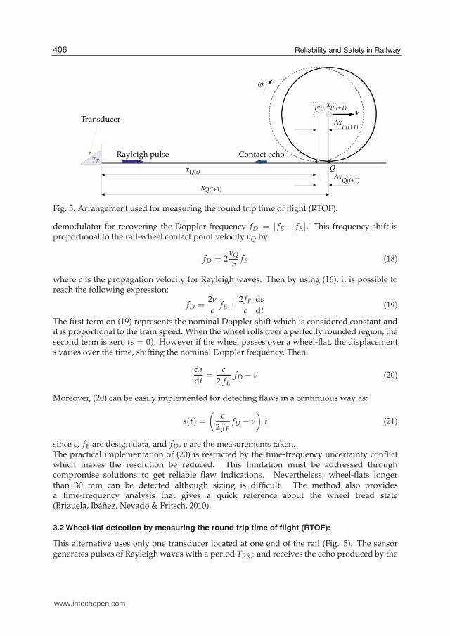
Fig. 5. Arrangement used for measuring the round trip time of flight (RTOF).

demodulator for recovering the Doppler frequency fD = | fE − fR|. This frequency shift isproportional to the rail-wheel contact point velocity νQ by:

fD = 2νQ

cfE (18)

where c is the propagation velocity for Rayleigh waves. Then by using (16), it is possible toreach the following expression:

fD =2ν

cfE +

2 fE

c

ds

dt(19)

The first term on (19) represents the nominal Doppler shift which is considered constant andit is proportional to the train speed. When the wheel rolls over a perfectly rounded region, thesecond term is zero (s = 0). However if the wheel passes over a wheel-flat, the displacements varies over the time, shifting the nominal Doppler frequency. Then:

ds

dt=

c

2 fEfD − ν (20)

Moreover, (20) can be easily implemented for detecting flaws in a continuous way as:

s(t) =

(

c

2 fEfD − ν

)

t (21)

since c, fE are design data, and fD, ν are the measurements taken.The practical implementation of (20) is restricted by the time-frequency uncertainty conflictwhich makes the resolution be reduced. This limitation must be addressed throughcompromise solutions to get reliable flaw indications. Nevertheless, wheel-flats longerthan 30 mm can be detected although sizing is difficult. The method also providesa time-frequency analysis that gives a quick reference about the wheel tread state(Brizuela, Ibáñez, Nevado & Fritsch, 2010).

3.2 Wheel-flat detection by measuring the round trip time of flight (RTOF):

This alternative uses only one transducer located at one end of the rail (Fig. 5). The sensorgenerates pulses of Rayleigh waves with a period TPRF and receives the echo produced by the


www.intechopen.com


moving rail-wheel contact point. The rail-wheel contact position obtained from measuringthe RTOF (TQ(i)) of a pulse i is:

xQ(i) =c TQ(i)

2(22)

where c also means the propagation velocity for Rayleigh waves. Assuming that the trainmoves at a constant speed ν; the wheel center projection over the rail for the same pulse i is:

xP(i) = i TPRF ν (23)

Therefore, the relative displacement between P and Q can be figured out as follows:

s(i) = xQ(i) − xP(i) =c TQ(i)

2− i TPRF ν (24)

On the other hand, a sampled system can approach the integration indicated on (15) as:

dk(M) =ν TPRF

R

k+M

∑i=k

s(i) (25)

where the differential on (15) has been replaced by ∆ϕ = ω ∆t = ν TPRF/R and M is thediscrete version of the angle ϕA. The sum given by (25) is extended over M samples of s(i)which is obtained from (24). Consequently, M should be chosen to cover at least half thelargest irregularity. Since the sampling period of s(i) is TPRF and Lmax is the length of thelargest wheel-flat of interest,

M ≥ Lmax

2 ν TPRF(26)

The measuring process (25) is carried out as a convolution of a rectangular unity window of Msamples with the values of s(i). This way M measurements of d are taken: the sequence dk(M)represents the value of the loss of material d, which is estimated by convolving the k with awindow of size M. Since the window must be wider than the irregularity, the peak value ofthis sequence corresponds to the best estimation of d for isolated wheel-flats. Fig. 6 showsgraphically the measuring process. For a given value of M samples, the resulting sequencedk(M) has two peaks, one negative dN followed by another positive dP, which correspond tothe lead-lag of P respect to Q on the signal displacement s. Their absolute values scaled bythe factor ν TPRF/R, make the result be equal to d. However in real applications where noiseis present, d can be much better estimated by the peak-to-peak average:

dE(M) =ν TPRF

R

|dP(M)|+ |dN(M)|2

(27)

Once the estimated value dE has been found, the length corresponding to the originalwheel-flat LE can be obtained by application of (1).This methodology also provides a suitable possibility of estimating the train speed requiredby (27). The contact point velocity is νQ = ν while the wheel rolls over a defect-free region,otherwise during an irregularity νQ �= ν. Nevertheless, the average speed along the wheel-flatis νQ = ν. Consequently, by calculating the contact point mean-speed for a long enough timeinterval the train speed is obtained with a good accuracy.


www.intechopen.com


0 50 100 150 200 250

−1

−0.5

0

0.5

1

(a) Displacement signal s

0 50 100 150 200 250

0

0.2

0.4

0.6

0.8

1

M

(b) Rectangular unity window w

0 50 100 150 200 250

−15

−10

−5

0

5

10

15 d

P

dN

(c) Resulting sequence dk = s ∗ w.

Fig. 6. Measuring process carried out as a convolution of s with an unit window of Msamples.

The contact point moves a distance ∆xQ(i) between two consecutive pulses. The xQ(i) positionis measured at a time:

t(i) = i TPRF +TQ(i)

2(28)

in the following interrogation pulse, the Q position is sampled at:

t(i+1) = (i + 1) TPRF +TQ(i+1)

2(29)

The elapsed time between measures (28) and (29) is:

∆t(i) = TPRF +∆TQ(i)

2(30)

The Q movement is:∆xQ(i) = νQ(i) ∆t(i) (31)


www.intechopen.com


At the same time, the ultrasound pulse has also to cover the distance advanced by the contactpoint, thus:

∆TQ(i) = 2∆xQ(i)

c(32)

where the constant c is the propagation velocity for Rayleigh waves on the rail. By replacing(31) on (32) and then combining on (30), it yields:

∆TQ(i)

(

c − νQ(i)

c

)

= 2νQ(i)

cTPRF (33)

where the factor (c − νQ(i))/c means a Doppler shift between the frequency at which theinterrogation pulses are emitted (1/TPRF) and at which they are received. As νQ(i) << c

it can be assumed that (c − νQ(i))/c ≈ 1. Therefore, the contact point velocity νQ(i) is obtainedfrom (33) as:

νQ(i) ≈∆TQ(i)

2 TPRFc (34)

where all values in (34) are known and ∆TQ(i) results from the difference of two consecutiveRTOF measures. The νQ(i) value represents the instantaneous velocity estimation of thecontact point by sending a pulse i. Afterwards, the train speed ν can be found out by averagingN measurements of νQ(i):

ν ≈ ν(j) =1

N

⎛

⎝

i=j+N−1

∑i=j

νQ(i)

⎞

(35)

Finally, the measuring process indicated on (27) only requires the knowledge of the wheelradius R, whose value may be smaller than the nominal one due to the wheel wear. Onthe other hand, the product ν TPRF = ∆x represents the spatial sampling interval whichdetermines the length resolution of the irregularity.

4. Measuring process simulation

In practical applications, signals are interfered by electrical and structural noise leading tovariations in the measured position xQ(i). Nevertheless the measuring method is very robustagainst noise due to the integration performed on (25).

Fig. 7(a) shows a simulated sequence s(i) corresponding to a degenerated wheel-flat with d= 0.4 mm in a wheel of R = 500 mm. It has been acquired at intervals ∆x = ν TPRF = 0.6mm in a rail with c = 3000 m/s. In order to test the technique performance, this sequencehas been deeply contaminated with white Gaussian noise and standard deviation increasingwith distance. The signal represents a typical acquisition when the Time-Gain-Compensation(TGC) function, on an ultrasound equipment, has been turned on to receive similar echoamplitudes from different distances . Interferences signify a considerable uncertainty infinding the actual echo position after every pulse i.

The resulting sequence dk obtained from the noisy signal s(i) by application of (25) is shownin Fig. 7(b). It has been used a window size of M = 267 samples, or following (26), thiscorresponds to a maximum wheel-flat length of Lmax = 320 mm. It can be seen the filteringeffect of the sum, as well as the agreement of the negative and positive peaks with the correctd = 0.4 mm value (dN = 0.3898 mm, dP = 0.4824 mm). The averaged estimation is dE =0.4361 mm.


www.intechopen.com


0 500 1000 1500 2000 2500 3000

−10

−8

−6

−4

−2

0

2

4

6

8

10

s [

mm

]

x [mm]

(a) Simulation of a noisy sequence s.

0 500 1000 1500 2000 2500 3000

−0.5

−0.4

−0.3

−0.2

−0.1

0

0.1

0.2

0.3

0.4

0.5

d

k [

mm

]

x [mm]

(b) Resultant dk sequence.

Fig. 7. Simulation parameters: R = 500 mm, c = 3000 m/s, d = 0.4 mm, and ∆x = ν TPRF = 0.6mm.

4.1 Choosing the integration window

In the case of a single wheel-flat, the M value must be strictly chosen greater than thenumber of samples obtained from a cycle of s in order to provide a robust estimation of d.However, for multiple wheel-flats which are frequently formed on modern high speed trainsdue to the failure of disc brakes and wheel slid prevention systems (WSP) (Grosse et al., 2002;Kawaguchi, 2006). In such case, a too large integration window may include informationbelonging to different flats giving wrong results.

Fig. 8(a) shows a simulated s sequence acquired at ∆x = 0.6 mm. The signal corresponds tothree degenerated wheel-flats of d = 0.5, 0.6, and 0.4 mm without overlapping (separated at 157mm) in a wheel of R = 500 mm. The resulting dk sequence using an integration window Mx =∆x M = 150 mm (distance less than wheel-flats separation) provides a wrong information,since no indication is given about the largest defect of d = 0.6 mm (Fig. 8(b)). These effects havebeen originated by the size chosen for the window Mx. So when the integration is performed,s values corresponding to consecutive wheel-flats are combined (note that first and last cycles,corresponding to the extreme flaws, have been correctly evaluated).

Repeating the same procedure but using a smaller window Mx = 75 mm (half of the previouscase), the resulting sequence dk contains information according to the loss of material d of eachwheel-flat: dN1

= 0.5107 mm, dP1= 0.4859 mm, dN2

= 0.5876 mm, dP2= 0.5485, dN3

= 0.4688 mm,dP3

= 0.3678 mm (Fig. 8(c)).

Therefore, the value of M should be determined by a heuristic process trying out differentintegration window sizes for each obtained signal s. From this process, it is interestingto know the greatest estimation which is linked to the deeper wheel-flat. Moreover, fromthe standpoint of railway maintenance, this value indicates whether the wheel should bereprofiled or removed from service. Fig. 8(d) shows the estimations resulting of trying outdifferent window sizes (1 ≤ Mx ≤ 150 mm) on the signal shown in Fig. 8(a). The maximumvalue provides an estimation of the greater wheel-flat characteristic: max [dE(M)] = 0.6326mm which is a value acceptably close to the real one (d3 = 0.6 mm).


www.intechopen.com


0 500 1000 1500 2000 2500 3000−15

−10

−5

0

5

10

15 s [

mm

]

x [mm]

(a) Simulation of a noisy sequence s.

0 500 1000 1500 2000 2500 3000

−0.5

−0.4

−0.3

−0.2

−0.1

0

0.1

0.2

0.3

0.4

d

k [

mm

]

x [mm]

(b) Sequence dk using Mx = 157 mm.

0 500 1000 1500 2000 2500 3000

−0.6

−0.4

−0.2

0

0.2

0.4

0.6

d

k [

mm

]

x [mm]

(c) Sequence dk corresponding to Mx = 75 mm

0 20 40 60 80 100 120 1400

0.1

0.2

0.3

0.4

0.5

0.6

0.7

d

E [

mm

]

Mx [mm]

(d) dE(M) estimated by a multiple windowsprocess.

Fig. 8. Simulation parameters: 3 wheel-flats without overlapping; loss of material for eachwheel-flat d = 0.4, 0.6, 0.5 mm; wheel radius R = 500 mm and ∆x = ν TPRF = 0.6 mm.

5. Prototype inspection system

An UltraSCOPE�, Dasel Sistemas (2010), ultrasonic testing instrument was modified tosupport this methodology. In order to optimize bandwidth and storage requirements, theacquisition time has to be kept small. Thus, a tracking algorithm was developed and hardwareimplemented to make a narrow acquisition window around the rail-wheel contact pointfollows the contact-echo displacement (Brizuela, Ibáñez & Fritsch, 2010).

On the other hand, the acquired signals are interfered by grain noise and many otherpropagation modes in the measuring rail, which cannot be removed by conventional filtering.Fortunately, this kind of noise can be partially removed because it is mostly static. Therefore,a noise cancellation procedure was also included with the tracking algorithm to avoid losingthe contact echo. To this purpose, a vector formed by the difference of the absolute valuesbetween two consecutive acquisitions is obtained. Electrical noise is also reduced by applyinga programmable narrow-bandpass 63-coefficients FIR filter.


www.intechopen.com


(a) Original A-scan. (b) Differential trace.

Fig. 9. Structural noise cancellation. In both cases the wheel is in motion near the same railregion.

Since the acquisition system operates over a differential trace, if the wheel is static ornon-present, A-scans will be null excepting the electrical noise. While the wheel is in motion,A-scans will contain the information about the actual rail-wheel contact point position as apositive indication and the precedent one with negative sign. While the acquisition windowis moving, the noise cancellation algorithm is performed using the samples which correspondto the same spatial point on the rail in consecutive acquisitions. Fig. 9(a) shows a high railstructural noise which masks the wheel contact-echo in the acquired signal. After structuralnoise removal, the wheel echo is clearly visible (Fig. 9(b)).

In addition other functions have been included, such as, Time-Gain-Compensation (TGC) toreceive similar contact-point echo amplitudes from different distances; a programmable burstgenerator to drive transducers through a power stage (pulser). Finally, measurements arelaunched automatically when a wheel is detected over the rail.

The recorded echo signals are sent through a USB 2.0 interface to an evaluation computer,which looks at the position of the signal value maximum in each capture to recover the RTOFTQ(i) required to compute s(i) and νQ(i) on eqs. (24) and (16).

5.1 Test bench

Finally, to evaluate the proposed technique performance, an experimental test bench wasarranged (Fig. 10(a)). A 1 MHz piezoelectric transducer generates Rayleigh wave pulses in a2000 mm long measuring rail. A pair of wheel treads with R = 420 mm were used to performthe experimental work.

Two artificial wheel-flats were mechanized, one on each wheel tread. Figs. 10(b) and 10(d)show the test profiles measured with a mechanical comparator (10(c)). The maximum loss ofmaterial for the wheel-flat #1 is d = 0.46 mm. By application of (1) this corresponds to a newwheel-flat length of L = 39.3 mm. A simple comparative between measured and new profilescan be also done in Fig. 10(b). Note that profile #1 corresponds to an asymmetric partiallyrounded wheel-flat.


www.intechopen.com


(a) Experimental test bench.

−40 −30 −20 −10 0 10 20 30 40

418

418.5

419

419.5

420

[mm]

[m

m]

Wheel profile

New wheel−flat profile

Measured wheel−flat profile

(b) Wheel-flat #1

(c) Mechanical measuring instrument.

−40 −30 −20 −10 0 10 20 30 40

418

418.5

419

419.5

420

[mm]

[m

m]

Wheel profile

New wheel−flat profile

Measured wheel−flat profile

(d) Wheel-flat #2.

Fig. 10. Prototype inspection system used for laboratory testing and artificial wheel-flatprofiles.

On the other hand, the wheel-flat #2 profile shown in Fig. 10(d), has a shape slightly concave(a cavity). This artificial flaw emulates a new wheel-flat, since it is not possible to roll over acavity. The corresponding new wheel-flat is defined by d = 0.20 mm which yields to a lengthof L = 25.9 mm.

6. Experimental results

The wheelset was moved by hand over the measuring rail, so that the speed was not quiteconstant. However, the rail-wheel contact position xQ(i) is obtained by (22) as a function of themeasured RTOF TQ(i) and the ultrasound propagation velocity c = 2970 m/s. Consequently,the mean speed ν can be also estimated for every position in the rail by applying (35).

The wheel-flat #1 was tried out under this procedure. The estimated mean speed near the flatregion was ν ≈ 0.45 m/s and the spatial sampling interval was ∆x = ν TPRF = 0.90 mm.Figure 11(a) shows the contact point distance xQ(i) as a function of the trigger number. Notethe jump in xQ when the wheel rolled over the wheel-flat, which is shown with more detail inFig. 11(c). The current wheel-flat length could be obtained from this graph by observing theslope of xQ which changes between triggers #820 and #860, that is, an interval ∆t = 80 ms at


www.intechopen.com


200 400 600 800 1000 1200 1400

400

600

800

1000

1200

1400

[m

m]

Trigger number

(a) Rail-wheel contact point position xQ .

200 400 600 800 1000 1200−20

−15

−10

−5

0

5

10

15

[m

m]

Trigger number

(b) Displacement signal s.

810 820 830 840 850 860 870 880

980

990

1000

1010

1020

1030

1040

[m

m]

Trigger number

(c) Detailed view of Fig. 11(a).

780 800 820 840 860 880 900

−15

−10

−5

0

5

10

15

[m

m]

Trigger number

(d) Detailed view of Fig. 11(b).

Fig. 11. Wheel position obtained by measuring the RTOF (TQ(i)) and the relativedisplacement between contact point and the wheel center projection as a function of thetrigger number.

TPRF = 2 ms. The wheel-flat length can be easily found out by multiplying the train speedν and ∆t, which yields to L ≈ 36.4 mm. Nevertheless, this measurement method is ratherimprecise, since it depends on finding the points where xQ changes its slope. Moreover, itgives no information about the dimensions of the original new wheel-flat (length and loss ofmaterial). Therefore, it is much better to estimate the original loss of material d by applyingthe area calculation on |s(i)|.Figure 11(b) shows the displacement s around the flat region computed by (24). This sequenceis contaminated by the uncertainty of locating the exact position of the echo signal due toresidual noise (Fig. 11(d)). Then, (25) was applied with different window widths (2 ≤ M ≤250 samples), obtaining dE(M) from (27).

Figure 12(a) shows the resulting estimation of dE as a function of M. It can be seen that,for M values below those indicated by (26), that is, M < 16, the estimated dE value showserrors. Above this figure, the estimation remains steady near the true value (0.46 mm), withan average dEmean

= 0.40 mm and a standard deviation σdE= 0.03 mm, in agreement with

theory. The maximum estimation is obtained when M = 27 (or Mx = 24.30 mm), where dE(27)


www.intechopen.com


50 100 150 200

0.1

0.15

0.2

0.25

0.3

0.35

0.4

0.45

0.5

M

[m

m]

(a) Estimated loss of material dE.

50 100 150 200

15

20

25

30

35

40

M

[m

m]

(b) Estimated new wheel-flat length LE.

Fig. 12. Loss of material d and new wheel-flat length LE estimations as a function of theintegration window size.

Parameter Wheel-flat#1 Wheel-flat#2

Loss of material d [mm] 0.46 0.20Equivalent new wheel-flat length L [mm] 39.3 25.9

Distance to transducer x [mm] 500 1000 2000 700 900 1300Mean speed ν [m/s] 0.33 0.45 0.54 0.21 0.25 0.34Sampling interval ∆x [mm] 0.66 0.90 1.62 0.42 0.50 0.68Highest estimation dEmax [mm] 0.45 0.48 0.56 0.21 0.20 0.16Mean estimation dEmean [mm] 0.40 0.40 0.40 0.17 0.16 0.15Estimated maximum length LEmax [mm] 38.90 40.75 43.72 27.07 26.16 23.57Relative error ε(LEmax)% -1.01 3.68 11.32 4.51 0.10 -8.99Estimated average length LEmean[mm] 35.40 36.61 40.30 24.14 23.02 21.06

Table 1. Wheel-flats evaluation at different distances from the transducer.

= 0.49 mm a value slightly higher than the measured value. In fact, it can be seen that using alarge value for M has little impact in the measurement of isolated wheel-flats.

Figure 12(b) shows the corresponding LE(M) values, using the estimations dE(M) and (1).The average value LEmean

is 36.61 mm with a standard deviation σLE= 1.39 mm. Note that

the equivalent new wheel-flat length is 39.3 mm. These results show a small error by defect,which are due to approaching the integral (15) by a sum (25). The maximum length estimatedis LEmax

= 40.75 mm and it is found at M = 27 as well.

Following this methodology, both artificial wheel-flats were evaluated in several positionsover the measuring rail in order to put them under different conditions of structural noiseinterference. On Table 1 the obtained results of these experiments have been summarized.Note that as the wheel speed has not been controlled, so the spatial sampling interval isdifferent for each test.

For all cases, the lower relative error with regard to the true value is reached when theintegration window extent is close to the defect length, so the estimation is maximum. Theerror increases when measurements are made beyond 1300 mm of the transducer, where


www.intechopen.com


Parameter Wheel-flat #1

Decimation factor n 1 2 3 4 5 6 7 8 9 10

Mean speed ν [m/s] 0.41 0.82 1.24 1.65 2.06 2.48 2.89 3.30 3.72 4.13Spatial sampling interval ∆x [mm] 0.90 1.82 2.72 3.63 4.54 5.45 6.36 7.27 8.18 9.09Window size M [samples] 28 14 12 9 7 6 5 5 4 4Estimated maximum length LEmax [mm] 40.75 40.09 40.60 39.47 39.29 37.72 37.64 41.43 42.32 42.93Relative error ε(LEmax)% 3.69 2.02 3.32 0.45 -0.01 -4.01 -4.22 5.42 7.68 9.25Estimated average length LEmean [mm] 36.42 35.94 35.90 34.77 38.38 36.90 37.13 34.42 34.37 34.05

Table 2. New wheel-flat estimated at different train speed using the recorded signal on Fig.11(b).

interrogation pulse attenuation is important and structural noise interferences on the echosignal are higher, increasing the error on determining the contact point position. Nevertheless,the estimated lengths corresponding to wheel-flat #1 have been obtained with a relative errorbelow 12%. On the other hand, detecting the wheel-flat #2 is more difficult because it issmaller. In this case, the amplitude of the displacement signal s is comparable to the residualnoise. However, lengths have been estimated with an error below 9%, which confirmsexperimentally the method robustness.

6.1 Measures under different speed inspection conditions

The technique behaviour has been also tested by making the measurements at multiple speeds(more than 3m/s). The recorded displacement signals were decimated in order to increase theequivalent wheel speed. Table 2 contains the wheel-flat length estimations corresponding tothe displacement signal shown in Fig. 11(b). In this case, the integration window size wasbounded to Mx = 150 mm. The maximum length estimated is obtained when the windowsize is close to the equivalent new wheel-flat length (39.9 mm), however fewer samples arecontained on M as the speed increases.

The estimated maximum lengths of the new wheel-flat at speeds up to 3 m/s remain close tothe true value with relative errors that do not exceed 5 %, which means an inaccuracy of 1.9mm. For higher train speeds the relative error increases because the spatial sampling intervalwill increase as well. Note also that, as the inspection speed increases the average wheel-flatlengths tend to decrease as a consequence of capturing fewer samples.

Consequently, inspection speeds that exceed a maximum value of 3 m/s should be avoidedto keep enough resolution.

7. Conclusion

Over this chapter, a new concept supported on a theoretical background has been disclosedto detect and measure wheel-flats in the rolling surface of railway wheels. Wheel-flats arequantified by the sum of relative displacements between the wheel-rail contact point and thewheel center projection on the rail, which yields the loss of material produced by abrasion inthe original flat formation. These displacements can be obtained from ultrasonic techniquesby analysing the contact point echo. Two methods based on the same measuring arrangementbut different principles have been described and discussed.


www.intechopen.com


In the first proposed method based on the Doppler effect, wheel-flats can be easilydistinguished. However, this technique does not allow measuring their length due to theuncertainty in the time-frequency analysis. Nevertheless, it provides a reliable wheel-flatindication, which can be very useful to give warning of failure.

On the other hand, the RTOF measuring alternative provides a high resolution which allowssizing wheel-flats. In this technique, the displacement signal s is obtained from the measuredRTOF and the wheel mean speed can be also estimated.

This methodology has been tested by simulation using high noise levels in signals andwheel-flats with different stages of roundness. The simulation results have proven that thistechnique is robust against noise and the measurement is independent of wheels wear degreeand wheel-flats roundness.

An experimental test bench was built to evaluate the technique performance. The specifichardware design provides a robust support for a quantitative measurement of wheel-flats,independently of the hostile railway environment, weather conditions and wheel wear. Twoartificial wheel-flats of 40 and 26 mm length with different wear degree were mechanizedin a railway wheelset for testing. The artificial wheel-flats were placed at different positionsover the measuring rail and the estimated lengths remained close to the true value with a lowrelative error. Thus, simulation and experimental results agree with the theoretically expected.

The inspection speed was also taken into account for the RTOF measuring method. Recordedsignals were decimated in order to increase the equivalent wheel speed. The system resolutiondecreases as the speed increases; nevertheless estimated lengths remained close to the realvalue with relative errors below 5% at maximum speed (3 m/s).

The proposed methodology, as being a dynamic technique without moving parts but with awell-characterized and stable measuring arrangement, is suitable for the railway industry. Thesystem allows a periodical wheel inspection, improving reliability, availability and effectiveoperations of the railway system, guaranteeing high safety standards. Moreover, it allowsreducing the maintenance costs. The inspection procedure can be performed while the trainis getting into a repair shop reducing the time spent in maintenance scheduled tasks. As aresult, frequently inspections can allow to follow-up the wheel wear history by uploading theinformation into a database and optimizing wheels service.

8. References

Baeza, L., Roda, A., Carballeira, J. & Giner, E. (2006). Railway train-track dynamics forwheelflats with improved contact models, Nonlinear Dynamics 45: 385 – 397.

Belotti, V., Crenna, F., Michelini, R. & Rossi, G. (2006). Wheel-flat diagnostic tool via wavelettransform, Mechanical Systems and Signal Processing 20(8): 1953–1966.

Bray, D., Dalvi, N. & Finch, R. (1973). Ultrasonic flaw detection in model railway wheels,Ultrasonics 11(2): 66–72.

Brizuela, J., Ibáñez, A. & Fritsch, C. (2010). NDE system for railway wheel inspection in astandard FPGA, Journal of Systems Architecture 56: 616 – 622.

Brizuela, J., Ibáñez, A., Nevado, P. & Fritsch, C. (2010). Flaw detector for railways wheels bydoppler effect, Physics Procedia 3(1): 811 – 817.

Dasel Sistemas (2010). Ultrasound technology. viewed March 22, 2012,http://www.daselsistemas.com.


www.intechopen.com


Fan, H. & Jia, H. (2008). Study on automatic testing of treads of running railroad wheels,Proceedings of the 17th World Conference on Nondestructive Testing, 17th WCNDT 2008,Shangai, China.

Feng, Q., Cui, J., Zhao, Y., Pi, Y. & Teng, Y. (2000). A dynamic and quantitative method formeasuring wheel flats and abrasion of trains, 15th World Congress on NDT, Rome,Italy.

Grosse, M., Ceretti, M. & Ottlinger, P. (2002). Distribution of radial strain in a disc-brakedrailway wheel measured by neutron diffraction, Applied Physics A: Materials Scienceand Processing 74: 1400 ? 1402.

Gutauskas, P. (1992). Railroad flat wheel detectors. US Patent No. 5 133 521.He, P., You, Z. & Teng, S. (2005). Fast algorithm of flat sliding detection in flat wheel detecting

system, Instrumentation and Measurement Technology Conference, IMTC 2005, Ottawa,Canada.

Ibáñez, A., Parrilla, M., Fritsch, C. & Giacchetta, R. (2005). Inspección mediante ultrasonidosde ruedas de tren en operaciones de mantenimiento, V CORENDE Proceedings,Neuquén, Argentina.

Kappes, W., Kröning, M., Rockstroh, B., Salzburger, H.-J. & Walte, F. (2000). Non-destructivetesting of wheel-sets as a contribution to safety of rail traffic, CORENDE 2000Proceedings, Mar del Plata, Argentina.

Kawaguchi, K. (2006). Development of a wsp system for freight trains, 7th World Congress onRailway Research (WCRR2006 Proceedings)., Montreal, Canada.

Kumagai, N., Ishikawa, H., Haga, K., Kigawa, T. & Nagase, K. (1991). Factors of wheels flatsoccurrence and preventive measures, Wear 144: 277 – 287.

Madejski, J. (2006). Automatic detection of flats on the rolling stock wheels, Journal ofAchievements in Materials and Manufacturing Engineering 16(1-2): 160–163.

Pohl, R., Erhard, A., Montag, H.-J., Thomas, H.-M. & Wüstenberg, H. (2004). NDT techniquesfor railroad wheel and gauge corner inspection, NDT&E International 37: 89 – 94.

Salient Systems, Inc. (2010). Intelligent track solutions. viewed March 22, 2012,http://www.salientsystems.com.

Salzburger, H. J., Wang, L. & Gao, X. (2008). In-motion ultrasonic testing of the tread ofhigh-speed railway wheels using the inspection system AUROPA III, 17th WorldConference on NDT, Shangai, China.

Snyder, T. & Stone, D. H. (2003). Wheel flat and out-of-round formation and growth, Proc.2003 IEEE/ASME Joint Rail Conf., Chicago, Illinois, pp. 143 – 148.

Stratman, B., Liu, Y. & Mahadevan, S. (2007). Structural health monitoring of rail road wheelsusing impact load detectors, Journal of Failure Analysis and Prevention 7(3): 218 – 225.

Vyas, N. S. & Gupta, A. K. (2006). Modeling rail wheel-flat dynamics, Engineering AssetManagement, Springer London, pp. 1222 – 1231.

Wu, T. X. & Thompson, D. J. (2002). A hybrid model for the noise generation due to railwaywheel flats, Journal of Sound and Vibration 251(1): 115 – 139.

Zakharov, S. M. & Goryacheva, I. G. (2005). Rolling contact fatigue defects in freight carwheels, Wear 258: 1142 – 1147.

Zerbst, U., Mädler, K. & Hintze, H. (2005). Fracture mechanics in railway applications – anoverview, Engineering Fracture Mechanics 72(2): 163–194.


www.intechopen.com

Reliability and Safety in RailwayEdited by Dr. Xavier Perpinya

ISBN 978-953-51-0451-3Hard cover, 418 pagesPublisher InTechPublished online 30, March, 2012Published in print edition March, 2012

InTech EuropeUniversity Campus STeP Ri Slavka Krautzeka 83/A 51000 Rijeka, Croatia Phone: +385 (51) 770 447 Fax: +385 (51) 686 166www.intechopen.com

InTech ChinaUnit 405, Office Block, Hotel Equatorial Shanghai No.65, Yan An Road (West), Shanghai, 200040, China

Phone: +86-21-62489820 Fax: +86-21-62489821

In railway applications, performance studies are fundamental to increase the lifetime of railway systems. Oneof their main goals is verifying whether their working conditions are reliable and safety. This task not only takesinto account the analysis of the whole traction chain, but also requires ensuring that the railway infrastructureis properly working. Therefore, several tests for detecting any dysfunctions on their proper operation havebeen developed. This book covers this topic, introducing the reader to railway traction fundamentals, providingsome ideas on safety and reliability issues, and experimental approaches to detect any of these dysfunctions.The objective of the book is to serve as a valuable reference for students, educators, scientists, facultymembers, researchers, and engineers.

How to referenceIn order to correctly reference this scholarly work, feel free to copy and paste the following:

Jose Brizuela, Carlos Fritsch and Alberto Ibáñez (2012). New Ultrasonic Techniques for Detecting andQuantifying Railway Wheel-Flats, Reliability and Safety in Railway, Dr. Xavier Perpinya (Ed.), ISBN: 978-953-51-0451-3, InTech, Available from: http://www.intechopen.com/books/reliability-and-safety-in-railway/ultrasonic-dynamic-technique-for-detecting-and-quantifying-railway-wheel-flats-

© 2012 The Author(s). Licensee IntechOpen. This is an open access articledistributed under the terms of the Creative Commons Attribution 3.0License, which permits unrestricted use, distribution, and reproduction inany medium, provided the original work is properly cited.

http://creativecommons.org/licenses/by/3.0

Date post:	02-Feb-2022
Category:	Documents
Upload:	others
View:	3 times
Download:	0 times

New Ultrasonic Techniques for Detecting and Quantifying ...

Documents