ISOTROPIC-NEMATIC-LIQUID CRYSTAL PHASE TRANSITION: A LATTICE MODEL -* 1 Abstract 2 2 Introduction 3 2.1 History of LC’s ...................................... 3 2.2 Generalities about LC’s .................................. 3 2.3 Chirality in LC’s and helical particles ......................... 6 3 Theoretical Model 8 3.1 Basics of the LC model .................................. 9 3.2 Generalisation to helicoidal particles .......................... 11 4 Computational Methods 12 4.1 General features of the code ............................... 12 4.2 Monte Carlo method and Metropolis algorithm ................... 15 4.3 Boundary Conditions ................................... 16 4.4 Heat capacity and order parameter ........................... 17 5 Results and Discussion 19 6 Conclusions and Outlook 22 Figure 1 Common liquid crystals ............................ 4 Figure 2 LC’s most common phases ........................... 4 Figure 3 Cholesterics and chiral molecules ....................... 6 Figure 4 Features and properties of cholesterics .................... 7 Figure 5 Modelisation of helicoidal molecules ..................... 12 Figure 6 Periodical Boundary Conditions ....................... 17 Figure 7 Rod-like systems reaching estationary phase ................ 20 Figure 8 Nematic - Isotropic phase transition ..................... 21 Figure 9 Heat Capacity .................................. 22 Figure 10 Order Parameter for Nematic - Isotropic phase transitions ........ 23 * Tutor: Giorgio Cinacchi. Departamento de Física Teórica de la Materia Condensada, Universidad Autónoma de Madrid, Madrid, España. 1
Transcript
I S OT R O P I C - N E M AT I C - L I Q U I DC R Y S TA L P H A S E T R A N S I T I O N : A
Figure 10 Order Parameter for Nematic - Isotropic phase transitions . . . . . . . . 23
* Tutor: Giorgio Cinacchi. Departamento de Física Teórica de la Materia Condensada, Universidad Autónoma de Madrid, Madrid,España.
1
abstract 2
1 abstractA study of the nematic-isotropic phase transition in liquid crystals is made here. Sincethis phase transition mainly involves the rotational degrees of freedom of the particles, theLebwohl-Lasher lattice model is used. Using an original computer code, it is reported on thephase transition that takes place in systems of rod-shaped particles arranged on a simple cu-bic lattice. The computer code written in this thesis implements the Monte Carlo method andthe Metropolis algorithm. The energy, heat capacity and order parameter are calculated asproperties that allow the characterisation of the phase transition and are found in very closeagreement with literature data. This proves the validity of the Monte Carlo computer codewritten. The latter thus forms the basis on which to build further developments, namely theextension of the lattice model to handle helicoidal particles and the study of the chiral nematicliquid-crystal phases exhibited by them. In this report, a few comments are made on thesefurther developments.
introduction 3
2 introductionIt is usual to distinguish among three possible states of matter (four if we include plasmastate): gas, liquid and solid. However, there has been a special emphasis in recent years onseveral materials whose properties cannot be classified entirely as belonging to just one of theclassic states of matter, such as liquid crystals, the topic of this thesis.
2.1 History of LC’s
Liquid Crystals (LC’s from now on) are materials that may flow like a liquid but at the sametime their molecules or components have orientational and/or (partial) positional order. Infact at high temperatures they become isotropic conventional liquids. Their history begins in1888, when an Austrian botanical physiologist named Friedich Reinitzer looked into variousphysico-chemical features that exhibited some derivatives of cholesterol. Before that, someresearch had already been done on how cholesterol changed its color depending on the tem-perature, but none of those scientists recognised it as a new phenomenon. Reinitzer foundout that cholesteryl benzoate does not melt as other materials do but instead has two differentmelting points at 145.5 oC and at 178.5 oC with clearly differentiable phases. He contacted OttoLehmann, a physicist from Aachen (Germany), who confirmed that within the range of tem-peratures between the two melting points, the material showed crystallites, what suggestedsome kind of global ordering or crystal structure rather than just an ordinary liquid. Reinitzerpresented these results at a meeting in Vienna in 1888 [1]. Reinitzer gave up the study ofthese materials (which Lehmann would call cholesteric liquid crystals in 1904) after discover-ing three major features of them: the existence of two melting points and the capacity of thesematerials to either reflect circularly polarized light and change the polarization direction ofincident light. Lehmann did comprehend it as a new phenomenon, so his research startedwith cholesteric benzoate, a material with capacity to flow and a partial crystalline order [2].Next years were spent on synthetizing new materials that showed this behavoir [3, 4].
It was not until 1962 that the development of flat panels for electronic devices became im-portant and the research on liquid crystals had an unexpected boost. In that year RichardWilliams, from RCA Laboratories, applied an electric field to a thin layer of a nematic liq-uid crytal (para-azoxyanisole of figure 1a, fairly similar to cholesterol derivatives) at a hightemperature to form a regular pattern. Meanwhile George H. Heilmeier used this very samemolecule to create a flat crystal-based panel to replace the cathode ray vacuum tube used intelevisions. Unfortunately, this material and most of those known by then required very hightemperatures to become liquid crystals, what made them unconvenient to use. NeverthelessJoel E. Goldmacher and Joseph A. Castellano found out that mixtures of what were callednematic materials (fully described in the subsequent section) with subtle differences in thenumber of carbon atoms yielded nematic liquid crystals at room temperatures ( 30 oC) [5], sothe entire field was enhanced. Moreover in 1969 Hans Kelker synthesized MBBA (figure 1b),one of the most popular samples in liquid crystal investigations [6], which is liquid-crystallineat ambient conditions.
The growth of the commercialization of these materials led to the investigation of morestable substances, mostly rod-like particles. Finally, the Nobel Prize was awarded in 1991 toPierre-Gilles de Gennes for "discovering that methods developed for studying order phenomena insimple systems can be generalized to more complex forms of matter, in particular to liquid crystals andpolymers"[7].
2.2 Generalities about LC’s
The various LC’s phases, as soon as they cannot be classified neither as ordinary liquids norcrystal solids, are called mesophases due to their intermediate behaviour, for a LC is a materialin which some degree of anisotropy is present in at least one spatial direction, together withproperties such as fluidity and ordered structure. Furthermore, LC’s can be distinguished bythe physical quantity that has the biggest effect over the system and its composition. This way,
we can divide LC’s into thermotropic, lyotropic and metallotropic phases, each one with its ownsubclasses [8]. However we will focus on thermotropic LC’s as far as this thesis is based onthem rather than the other categories. We shall explain briefly some characteristics of each ofthe above-mentioned categories with special interest in thermotropic LC’s, and within them,nematics and cholesteric phases will occupy the most relevant part of our treatment.
1. Metallotropic LC’s: Composed by low-melting inorganic molecules like ZnCl2 in ad-dittion to other soap-like molecules, their properties depend on the organic-inorganicmolecules ratio and the temperature.
2. Lyotropic LC’s: Consist of organic macromolecules that act as LC’s mixed with solventmolecules filling the space around and giving fluidity to the system, so the propertiesvary with the concentration of particles and the temperature.
3. Thermotropic LC’s: Formed by organic molecules, temperature is the physical quantitythat drives the liquid-crystal phase behaviour.
For each of these groups, phases can be nematics, smectics or columnar. The different types ofmesophases can be distinguished by three characteristics: positional order, orientational orderand lenght-scales over which these types of order exist. These characteristics tell us whetherthe molecules have a partially positionally ordered arrangement, whether the particles arepointing toward the same direction and if this order is extended only to short distances (short-ranged) or to macroscopic lenghts (long-ranged). This gives rise to the next three categories:
(a) Nematic phase (b) Smectic A (c) Columnar phase(top view)
(d) Columnar phase (sideview)
Figure 2: Common liquid-crystal phases. Images were obtained using the free software QMGA(qmga.sourceforge.net).
2.2.1 Nematics
The word for nematics comes from the Greek νηµα which means thread because of the thread-like shape of some defects observed in these materials. Nematics show anisotropic positionalshort-range order but orientational long-range order. This means that a nematic material doesnot organize its molecules on the sites of a lattice but they are disordered in space, whereasalmost all of them share a preferential direction for their orientation, as seen in figure 2a.
introduction 5
molecules Tipically rod-shaped particles have played a main role in the development ofnematics, although there are also some cases in which disk-like or rectangular particles formthe nematic phase so instead of a uniaxial particles there may be a biaxial nematic. Howeverwe will limit ourselves to the uniaxial cases. We have already seen some of the most knownrod-shaped molecules that form a nematic phase in figure 1. For example, p-azoxyanisole(PAA) can be considered as a rigid rod of around 20 A long and width 5 A. Recalling thehistory of LC’s explained above, we saw PAA turns into a LC only at high temperatures(between 116
oC and 135oC) so the discovering of MBBA, which reaches that phase at room
temperature (20 - 47oC) was regarded as a great advance in the experimentation on LC’s. But
MBBA is not so stable as it would be desired, so nowadays it is more common to use othermolecules such as cyanobiphenyls and cyanobicyclohexyl derivatives for these compounds arechemically more stable.
properties There are some features that are remarkably important in nematics so theydefine whether or not a material is nematic:
1. Molecules have no long-range positional order. This characteristic is also shared withconventional liquids and allows for the fluidity of nematics.
2. On the other hand, molecules have directional long-range order along a director vector n,common for all the particles and semi-arbitrary in space (its direction is given by minorforces like the effect of the walls). All the molecules are completely symmetrical about arotation around n. Nematics tend to flow in the direction given by this director.
3. There is no difference in the system between a director vector n or -n.4. A very important feature as we shall see in the next section is that nematic phases are
only present in systems where each constituent is identical to its mirror image, thatis achiral. There are some cases where chiral particles present nematic behaviour, butonly if there is the same proportion of left-handed and right-handed molecules withinthe system. Actually, to a good degree of accuracy, cholesterics and nematics differalmost only in the chirality of their components but this has profound consequencies onthe structure of the phase. However, particle chirality is a necessary but not sufficientcondition for phase chirality.
2.2.2 Smectics
Its name comes from the Greek word σµηγµαwhich means soap. Smectics are usually presentat lower temperatures than nematics, and at the same time represent more ordered systems,defined by one-dimensional quasilong-range order. Smectics are formed by layers of materialwith orientational order but often no positional order within the layers and with a interlayerspacing ranging on the order of the size of the constituent molecules. We shall concentrateonly on the most important classes of smectics known currently: smectics A (figure 2b) andsmectics C, which differ only on how close are the orientations of the particles to a vectorperpendicular to the layers. Smectics A align normal to the surface of the layers, but smecticsC are slightly tilted by a small angle. In particular, if the particles that form a smectic C are notequal to their mirror image, and helicoidal smectic C* appears. In fact, as we will see below,chirality has a huge impact on the behaviour of liquid crystals, even giving rise to new phaseslike cholesterics.
2.2.3 Columnar phases
These are two-dimensionally ordered systems in three dimensions so they form ordered tubesas long as they are composed of stacked piles of discoidal organic molecules like hexasub-stituted phenylesters. A visual representation is showed on figures 2c and 2d. They havethree-dimensional long-range order just as a solid crystal does but molecules can move alongthe columns, the latter making a motion resembling that of sliding doors.
LC’s are not just an academical topic, for the uses and applications of LC’s are many: ly-otropics are fundamental phases in living systems as soon as cell membranes and proteins are
introduction 6
made of phospholipides and similar molecules, which form lyotropic LC’s. On the other hand,nematics are basic components of modern electronic devices, and most of the screens and pan-els seen daily around us are made of LC’s due to their extraordinary optical properties. Otherthermotropic mesophases are cholesterics, which can be a good representation of the DNA atsome stages of its development, and where the chiral nature of the constituent molecules playa major role on their properties.
2.3 Chirality in LC’s and helical particles
As we have seen previously, twisted molecules confer special properties to a LC material andlead to new phases, in particular state C* in smectics C and cholesterics, if we think of themas a special case of nematics (in fact, we shall see that except for the case when the pitch p istoo small, cholesterics can be viewed as twisted nematics). Smectics C* and cholesterics differin the orientational and positional order of the molecules. As the rest of smectics, smectics C*show the molecules arranged in layers but with every particle aligned to the same direction,whereas cholesterics show no long-range positional order within each layer, each of themoriented by a director vector that changes among layers, as can be seen in figure 3a.
(a) (Left) Cholesteric phase of rod-shaped particles. (Right) Cholestericphase of helix-shaped particles. Images obtained using the freesoftware QMGA
(b) General formula of a cholesterol estermolecule.
Figure 3: Rod-like and helical particles in a cholesteric and a chiral molecule that forms this phase.
From now on we shall concentrate on cholesterics, named this way because this phasewas first observed for cholesterol derivatives. Cholesteric mesophases need the constituentmolecules to have chirality i.e. the particle is different that its mirror image, although it isa necessary condition but not sufficient. Most usual molecules in cholesterics are cholesterolesters, whose general formula is showed in figure 3b. The molecular rings are not aromatic andthe structure is not planar but the rings are rigid and the edges of the particle act somehow asflexible tails.
Cholesterics and nematics can be viewed (in a very general way) as two subclasses of thesame mesophase, but nematics need achiral molecules or a racemic combination (1:1) of left-handed and right-handed species, and cholesterics can only take place if the molecules arechiral. Due to this fact, whereas nematogens (molecules of the nematic) align with respect to
introduction 7
a fixed director vector n in space (usually Z direction is taken as reference), cholesterics alignfollowing a director vector that we will call n that is not fixed in space but rotates betweenlayers of the material (see figures 3a and 4a) following the general expression
nx = cos (q0z+φ) (1)
ny = sin (q0z+φ) (2)
nz = 0 (3)
Where q0 has units of m−1. We shall call pitch p the distance over which the LC moleculesundergo a full 2π twist. Because the directions given by n and -n are equivalent, the structurerepeats itself every π radians. This pitch changes with temperature, something that makesthese materials quite interesting from the point of view of their optical properties. Typicalvalues of the pitch are in the range of around 3000 A, much larger than molecular dimensionsbut of similar lenghts of optical wavelengths, resulting in Bragg scattering of light beams.
(a) Structure of a cholesteric. (b) Free energy as a function of twisting q. (top)Nematic phase. (down) Cholesteric phase.
Figure 4: Properties of the cholesteric mesophase. Notice that a cholesteric is defined by the twisting ofthe particles vector and the length of the pitch, which depends on the temperature.
Because of the periodicity of these structures, the pitch can also be written in the followingway:
p =2π
|q0|(4)
The magnitud |q0| allows to look into various features; for example, the sign of q0 distin-guishes between right-handed and left-handed helical molecules, and at a given temperaturethe sign is always the same for a sample. Actually it may happen that at a certain temperatureT, the sign changes. In that very temperature, the system behaves like a conventional nematicmesophase, and once that point is crossed, the physical properties remain almost unchanged.
Previously we said that in cholesterics it is mandatory not to be racemic, i.e. to have sameproportion of left-handed and right-handed particles impedes the formation of this mesophase.Figure 4b presents the free energy per unit volume F as a function of q, the wavevector definedby the general formulas 1, 2 and 3, i.e:
q =∂θ(z)
∂z, (5)
with θ(z) = qz + φ. If the constituent molecules of the material are achiral so the imageof a given particle is the same as that of its mirror image, the free energy function F(q) issymmetrical and then F(q) = F(−q). In nematics, the minimum is located at q = 0, as seenin the upper curve in figure 4b. On the opposite side, if the molecules are chiral F(q) is notsymmetrical and the minimum value of F(q) does not fall at q = 0. This case corresponds tocholesterics, shown in the lower curve of figure 4b.
theoretical model 8
3 theoretical modelWe would need a consistent mathematical model if we would like to describe with a gooddegree of accuracy any physical system. In order to do that, we shall explain two conceptsthat will reveal themselves as fundamental in our treatment of LC’s: the existence of a directorvector and an order tensor [8]. Both will allow us to define any LC nematic system.
order tensor Assuming that the molecules within the LC are rigid rod-shaped, we canintroduce a unit vector u(i) along the axis of the ith molecule which describes its orientation.It is not possible to introduce a vector order parameter analogous to the magnetization vectorin ferromagnetic materials. Rather, a second-rank tensor appears to describe the ordering inLC’s, and its expression is given in equation 6 .
Qαβ(r) =1
N
N∑i=1
(u(i)α u
(i)β −
1
3δαβ
)(6)
where the sum is over all the N molecules in the volume located at the point r: indexesα,β = (x,y, z). There are some properties that make this order tensor interesting to describe aphysical system:
1. As soon as the product u(i)α u(i)β = u
(i)β u
(i)α and δαβ = δβα, it is trivial to show that Qαβ
is a symmetric tensor so:Qαβ = Qβα (7)
2. It is traceless, i.e. its trace Tr(Qαβ) is equal to zero since u is a unit vector:
Tr(Qαβ) =∑
α=(x,y,z)
Qαα =1
N
∑i
[(u(i)x
)2+(u(i)y
)2+(u(i)z
)2−1
33
]= 1− 1 = 0 (8)
This way we pass from a 3 x 3 matrix with 9 independent elements to only 5 elements.3. In the isotropic phase Qαβ = 0. It is easy to understand since every molecule of the
system points to a different orientation, making the average global order vanish.4. In a perfectly aligned nematic phase in which the molecules tend to align along the z
axis,
Q =
−1/3 0 0
0 −1/3 0
0 0 2/3
(9)
These properties tell usQαβ is a very good candidate to describe the order parameter of ourLC systems. It is zero in the isotropic phase when the LC behaves in a conventional liquid-likeway. This tensor is also very sensitive to the average orientation of the constituent molecules.The next question is: how do we know which is the preferred orientation direction of themolecules? The answer is given by the director vector.
director vector It is a feature of special interest in cases where global degree of orderingis not changing very much and therefore only the average orientation of the molecules hasa clear defined meaning. The order tensor explained above can be diagonalised for specificCartesian coordenate systems. Once it is diagonalised, we will mainly pay attention to thebiggest eigenvalue and its associated eigenvector, since the first one yields a way of measuringthe degree of alignment of the molecules with respect to the director vector n(r). Actually ifwe denote the biggest eigenvalue by λB, the value 32λB can be taken as the order parameter S,a scalar quantity that meassures the degree of global ordering. It is worth noticing that it isthe same to work either with the vector n or -n, for there is no physical polarization along thisaxis.
theoretical model 9
3.1 Basics of the LC model
At this point we are ready to introduce theories based on the features explained before (ordertensor and director vector): we shall begin with a cursory descriptionof the Onsanger theoryand Flory model, and after that the Maier-Saupe will be explained briefly in order to finish thesection with a full description of the Lebwohl-Lasher model.
It is worth noticing that all of the theories we are considering are based on statistical physicsand because of that each model has to characterise both the molecules and the interactions.Actually all of them consider the interactions among molecules as mean-field forces wherethe correlations between two molecules are not studied separately but a mean value of theirinteraction is taken into account to calculate the macroscopic properties of the system.
3.1.1 Onsanger’s theory and Flory’s model
It is possible to experimentally prepare solutions of hard-rod macromolecules whose length Land diameter D are well defined. Even in natural biological systems we can find these kind ofmolecules, for example Tobacco Mosaic Virus (TMV). The following assumptions were made in1949 by Onsanger [9] as fundaments of a statistical theory for LC’s:
1. Rods can not interprenetate each other. The only forces of importance are those cor-responding to steric repulsions (and if desired, Coulumb repulsion between chargedrods, even though this can be taken into account effectively by increasing the size of theeffective diameter of the molecules).
2. If we call c to the number density of rods, the volume fraction Φ = 14πcLD
2 is muchsmaller than unity.
3. The rods are very long so L >> D.
4. Let’s call cfadΩ the number of rods per unit volume pointing in a small solid angle dΩaround a direction labelled by the unit vector a. The sum of these solid angles overallwill give the total concentration c: ∫
fadΩ = 1 (10)
With these assumptions it is obtained a non-linear integral equation, and depending onthe ratio ΦL/D, it can give rise to anisotropic solutions. We simply recall that the Onsangersolution leads to an sharp transition between the ordered nematic phase and the isotropicconventional liquid phase. On the other hand, the hard rods become "athermal" molecules inthis model, which is valid for colloidal (lyotropic) LC’s.
The point of view adopted by Flory [10] was similar to the Onsanger one but with subtledifferences: instead of rigid rod-like molecules, a rod is described as a set of points inscribedon a lattice, and the number density of points acts just the same as the ratio L/D. The interestfor this model comes from that it is possible to calculate exactly the partition function of thesystem, something that can not be achieved in Onsanger’s theory. In fact the Onsanger theoryand the Flory’s model complement each other but fail when trying to account for the systemproperties along the entire range of possible c’s.
3.1.2 Maier-Saupe Theory
This theory was developed by Alfred Maier and Wilhelm Saupe and can be regarded as theanalogous in nematics of the approximation made by P. Weiss to describe ferromagnetics [11].There are slight differences depending on wheter the molecules are uniaxial or biaxial, but weshall focus on the uniaxial case as far as that is the shape of the molecules of our model.
Instead of considering the interaction due to every molecule of the volume this model worksthrough a mean-field average of these interactions. The details of the calculations can be foundin [8] and [11]. We will not go further into calculations since the purpose of this thesis is touse the Lebwohl-Lasher model to simulate a LC phase system, which can be considered as
theoretical model 10
the lattice version of the Maier-Saupe model. The latter theoretical model yields a thresholdtemperature Tc defined by equation 11 and an associated value of the order parameter justbefore the phase transition.
kBTc
U(Tc)= 4.55 (11)
where U(Tc) is the energy of the system at temperature Tc. In the original presentation it wasassumed that U is due entirely to van der Waals forces. If the temperature of the system T
is below Tc, the nematic phase is the stable one. The higher the temperature rises, the moredisordered the system becomes until the system is completely isotropic and behaves like aconventional liquid. The order parameter for T just below Tc is
Sc ≡ S(Tc) = 0.44 (12)
This equation yields a universal value for the order parameter at the phase transition. Thishas been in part confirmed by experiments on thermotropic nematics [12, 13].
3.1.3 Lebwohl-Lasher Model
This model, which we shall call LL from now on, is particularly useful in the description ofLC’s. It is a lattice version of the Maier-Saupe theory previously mentioned [14, 15]. It is theone we have used in this study. In the LL model, molecules are placed on the sites of a simplecubic lattice and described by an unit vector representing the orientation of each one of thesemolecules. The interaction among particles is expressed by the equation 13 which is a pairpotential restricted to first nearest neighbours.
H = −ε0∑i,j
P2(cos (θi,j)
)(13)
where ε0 is an energy parameter that measures the strenght of the interaction, and P2(cos (θi,j)
)is the second Legendre polinomial with θi,j the angle between two nerby orientation vectors(equation 14).
P2(z) =1
2
(3z2 − 1
)(14)
It is a matter of convenience to define a set of normalised adimensional units. In order todo so, we shall set the value of ε0 = 1, so from now on, we shall work in units of normalizedtemperature T∗ defined by:
T∗ =kBT
ε0(15)
This makes possible to work with adimensional units for the energy too.Beside these considerations about the description of the molecules and their interactions,
we need to consider which boundary conditions are useful as we will investigate this modelvia a numerical simulation method. In the LL model periodical boundary conditions areused. These conditions lack of physical significance but in some way make the lattice expandto infinite and avoid surface effects. Actually what we do is to establish our built lattice as abuilding block of a bigger system; this way the molecules of one edge surface will interact withtheir first neighbours, which will be in the very same state as the molecules on the oppositeedge surface.
This model has become a prototype for computer simulations on systems which undergoa nematic-isotropic-like orientational phase transition. Its role is fairly similar to the one thatIsing and Heisenberg models play in magnetic phase transitions. Note that in the case ofIsing magnetism, we only deal with spins with two possible states whereas in the LL model aparticle can have any orientation, defined either by two polar angles θ and φ. Thus, computercalculations are heavier to run, as long as for example we have to restrict ourselves to smallsystems with a volume size of around 30 x 30 x 30 molecules instead of the million particlesimulations that are possible for the Ising model [16].
theoretical model 11
3.2 Generalisation to helicoidal particles
In order to handle helicoidal particles and characterise the chiral nematic liquid-crystal phasesthat these sort of molecules undergo [17], a series of modification must be done on the previousmodel, namely the change in the shape of the molecules, no longer rod-like but helix-like,and because of it also the pair interaction among molecules must change. Additionally, newboundary conditions are required for the chiral nematic phases to take place.
new molecular shape Every unit vector we are considering as the orientation vector ofevery molecule must now take an helix-like shape, and ought to be able to rotate along themain axis of the molecule as rod-like molecules do. From a computationally point of view therequired steps are listed below:
1. Every rod-like molecule is divided into N equal segments of length L/N being L the totallength of the rod, in our case we can set L = 1. We can think of this stage as the passagefrom a single-unit to a multi-unit rod.
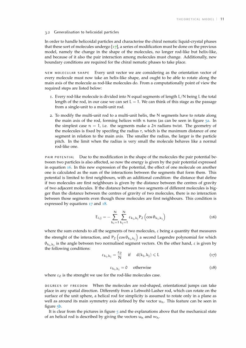
2. To modify the multi-unit rod to a multi-unit helix, the N segments have to rotate alongthe main axis of the rod, forming helices with n turns (as can be seen in figure 5a. Inthe simplest case n = 1, i.e. the segments make a 2π radians twist. The geometry ofthe molecules is fixed by specifing the radius r, which is the maximum distance of onesegment in relation to the main axis. The smaller the radius, the larger is the particlepitch. In the limit when the radius is very small the molecule behaves like a normalrod-like one.
pair potential Due to the modification in the shape of the molecules the pair potential be-tween two particles is also affected, so now the energy is given by the pair potential expressedin equation 16. In this new expression of the potential, the effect of one molecule on anotherone is calculated as the sum of the interactions between the segments that form them. Thispotential is limited to first neighbours, with an additional condition: the distance that defineif two molecules are first neighbours is given by the distance between the centres of gravityof two adjacent molecules. If the distance between two segments of different molecules is big-ger than the distance between the centres of gravity of two molecules, there is no interactionbetween those segments even though those molecules are first neighbours. This condition isexpressed by equations 17 and 18.
Ei,j = −
N∑ki=1
N∑kj=1
εki,kjP2
(cos θki,kj
)(16)
where the sum extends to all the segments of two molecules, ε being a quantity that measures
the strenght of the interaction, and P2(
cos θki,kj)
a second Legendre polynomial for whichθki,kj is the angle between two normalised segment vectors. On the other hand, ε is given bythe following conditions:
εki,kj =ε0N
if d(ki,kj) 6 L (17)
εki,kj = 0 otherwise (18)
where ε0 is the strenght we use for the rod-like molecules case.
degrees of freedom When the molecules are rod-shaped, orientational jumps can takeplace in any spatial direction. Differently from a Lebwohl-Lasher rod, which can rotate on thesurface of the unit sphere, a helical rod for simplicity is assumed to rotate only in a plane aswell as around its main symmetry axis defined by the vector uh. This feature can be seen infigure 5b.
It is clear from the pictures in figure 5 and the explanations above that the mechanical stateof an helical rod is described by giving the vectors uh and wh.
computational methods 12
(a) Helical molecule formed bytwisted segments. The orienta-tional state of the molecule isdefined by two normal vectors,uh and wh.
(b) Degrees of freedom of one molecule. It canrotate only on the plane YZ and around itsmain symmetry axis uh.
Figure 5: Modelisation of a helix-like molecule.
boundary conditions When the pitch of a helix is unknown or even temperature depen-dent, usage of periodic boundary conditions may introduce "frustation" effect, that can causethe system to choose the wrong phase entirely and discontinuos changes in the pitch. A new,self-determined boundary-conditions are required which are known as "spiraling boundary con-ditions" [18].
4 computational methodsThe aim of this section is to explain the original C++ code we have built and used to obtainthe results that are presented in the next section. In order to make it clear, here we shallpresent how the different parts of the model are implemented, showing some lines of the codewhen required. The simulation requires the files "nematics.cpp" and "functions.h". The first oneincludes the main body of the code, with the implementation of the model system, the identifi-cation of all the particles, the equilibration of the system through the Monte Carlo method andthe calculation of some properties of the system that cannot be processed through an externalfunction. When it was possible, those functions were written in the latter file, which containsthe implementation of Marsaglia’s pseudo-random number generator, the calculation of thechange in energy per particle, the Monte Carlo algorithm itself, and the routines for a coupleof properties such as the calculation of the order tensor Qαβ.
4.1 General features of the code
We have used the programming language C++ to build an original code based on arrays andpointers that implements a Monte Carlo numerical simulation for a 20 x 20 x 20 sized lattice.
As in all the theories explained in the previous section, our molecules will be defined asrigid rods, using time-dependant unit vectors to modelize them. So built, the molecules lackof diameter and then they represent infinitely thin rods. The interaction among particles followthe rule given by equation 13, with the potential restricted to first neighbours. Beside that, wework with the normalised and adimensional units defined by the normalised temperature ofequation 15. We have also taken kB = 1 for the sake of simplicity, and from now on theenergies will be normalised by dividing by the factor ε0 present in the pair potential.
computational methods 13
The initial configuration of our model can be of our choice. Three possibilities were consid-ered:
1. To start from a perfectly aligned arrangement of molecules. All of them point towardsthe z-axis with no deviations.
2. To start from a series of molecules with their orientation vectors distributed pseudo-randomly over the unit sphere. To achieve this we make use of Marsaglia’s pseudo-randomnumber generator, which will be explained in detail below.
3. From a previous configuration. It implies to save the vectors of a previous configuration,load them and restart the system from that point.
Before going further into the description of these possibilities, we shall present how weordered the coordinates of the 8000 molecules to arrange them into fixed positions on thelattice and to associate with each of them an energy and an orientation vector. It is shownbelow the code for this feature:
1 const unsigned int N = 20;
2 int Npart = N*N*N;
3 int coord[Npart][3]; //Coordinates of the 8000 particles
4 int ident[N][N][N]; //Auxiliar number to asign a number 0-7999 to each particle
5 for (int i=0;i<N;i++)
6 for (int j=0;j<N;j++)
7 for (int k=0;k<N;k++)
8 ident[i][j][k] = i+N*j+N*N*k;
9 coord[ident[i][j][k]][0] = i;
10 coord[ident[i][j][k]][1] = j;
11 coord[ident[i][j][k]][2] = k;
12
13
14
15 double u[Npart][3]; //Array of orientations
As can be seen, every molecule has an associated identity number between 0 and 7999. Thatnumber depends on the coordinates of each particle (line 8). The arrays called coord and ustore a three dimensional vector with the spatial coordinates and the unit orientational vectorsof each particle, respectively. This identifier number is also valid in the Monte Carlo method,allowing us to pick a particle and access to its properties immediately.
aligned vectors In the simulations we follow the general convention, and the moleculesare aligned along the Z-axis. This will be the configuration of minimum energy of the system,for the scalar product between parallel vectors is equal to the unity, and all the orientation vec-tors are aligned along the very same direction. It is clear that this is also the configuration withthe higher degree of symmetry, so the order parameter should be maximum. It correspondsto a perfect nematic phase, and is only stable at vanishing temperatures.
randomly on the unit sphere Here it is required to present a fully explanation of theMarsaglia method for the generation of pseudo-random numbers on the unit sphere. Withinthis algorithm we chose two pseudo-random numbers, let’s call them x1 and x2 which arein the interval [−1, 1]. To obtain these numbers we make use of the simple rand() functionalready avalaible in C++, and stating the seed of the pseudo-random number generator ona null time pointer. We shall restrict these two numbers to the interior of the unit circle, sonumbers which do not fulfill the constraint x21 + x
22 < 1 are automatically rejected. After
that, we simply make use of the formulas suggested by Marsaglia (lines 7,8 and 9). The threepseudo-randomly generated numbers are saved into a three dimensional array v. The entirealgorithm is shown below:
We cannot simply pick three numbers from the pseudo-random number generator functionrand() included in the standard library of the language because doing so would imply thatstatistically we would find that most of our vectors are poiting towards the poles of the unitsphere.
loading a previous configuration The Monte Carlo algorithm implies very heavy cal-culations and many time steps (of the order 105 at least), so it is really useful to run the codeonce and save the configuration so it is possible to re-run the code again but starting from aconfiguration that is closer to, or already has reached the equilibrium, speeding up the timeof convergence of the method. The way we achieve this is simply by saving the 8000 orienta-tion vectors on an external file that can be loaded when the program is run. The code itselfdetects if the file exists, so if it does not and the program cannot load a previous configura-tion, instantly the system is reinitialized to either an aligned system or a pseudo-randomlydistributed on the unit sphere.
In all of these cases, after setting the array of orientational vectors u, it is still necessary tocalculate the average normalised energy per particle < U∗ >/N. In order to do so, the fol-lowing algorithm calculates the energy due to the first neighbours of a given molecule. Theimplementation operates over the i,j and k directions separately. Here we present the functionfor the i-axis, the others being analogous:
Between lines 9 and 14 we can see the implementation of periodical boundary conditions. Wewill come back to them later. In the code above it is important to notice the contribution fromthe neighbours through the pair potential given in 13 in line 21. The exit value of the functionis the value of the energy difference between the old and the new states of the molecule. Thiswill be later explained better within the Monte Carlo section. This function can be appliedin any situation in which the orientations of the particles are well defined, so these two stepstogether are the previous and required step before applying the Monte Carlo algorithm. Oncewe know the orientation vectors and the total energy of the system, we can proceed to the nextstage.
4.2 Monte Carlo method and Metropolis algorithm
The entire thesis is based on the application of the Monte Carlo method to a physical modelsystem in order to simulate the behaviour of a corresponding real system. In what follows, weshall constraint ourselves to systems in which number of molecules (N), the total volume ofthe system (V) are fixed for a given temperature T .
Suppose we call by A a given observable of the system. The classical thermal average of Ais given by
< A >=
∫dpNdrNA
(pN, rN
)exp
[−H
(pN, rN
)/kBT
]∫dpNdrN exp
[−H
(pN, rN
)/kBT
] (19)
where the quantity Q, defined by the expression 20 is the partition function of the system,with rN being the coordinates of all the particles, pN their corresponding lineal momenta andH the Hamiltonian of the system:
Q = c
∫dpNdrN exp
[−H
(pN, rN
)/kBT
](20)
where c is simple a normalisation constant. When we want to obtain an average of a quantitythat depends on the position of the particles the problem becomes usually impossible to solveby brute force [19]. This trouble gave rise to more creative ways of solving it, and one of themhas become especially important: the algorithm proposed in 1953 by Metropolis et al [20], orimportance sampling algorithm.
The original paper suggested that it was possible to create a general algorithm (and infact, they did develope it) valid to calculate the properties of systems formed by individualmolecules that interact among themselves. The details of the mathematical demonstration arecontained in the literature above mentioned, and we shall only comment the features thatare most important for our system. Esentially the algorithm determines whether a virtualmovement of molecules within the system can be considered as a new stable state. The stepsto follow in the method are the following:
1. A random trial move is made on a particle of the system. In our case,the molecules arefixed at the sites of a lattice, but it is the orientation vector of one chosen molecule whatchanges. We have considered completely random orientational jumps.
2. Calculate the the change in energy due to this new configuration, ∆E.
3. In case the new configuration is more stable to the previous one, ∆E < 0, the system isbrought to a state of lower energy and the move is accepted.
4. If on the opposite side, ∆E > 0, we allow the move with probability exp (−∆E/kBT).In order to do that, we define a new random number ζ between 0 and 1, and if ζ <exp (−∆E/kBT) the move is accepted and the system is brought to the new configuration,even though it was not energetically favourable.
5. If the probability given by ζ is larger than the exponential, the move is rejected and thesystem goes back to the old configuration.
computational methods 16
A very interesting thing of this method is that, either the move is accepted or rejected in atime step, it is equally considered for the global properties of the system. Now we present thecomplete algorithm we have created and which has allowed to obtain all results shown later:
1 double monteCarlo(double u[8000][3],int
2 coord[8000][3],int ident[20][20][20],const unsigned int N,double T)
If we look at line 12 of the code above, we will find that when we change the orientation ofa particle, we do it by adding a unit randomly generated vector to the original one and thenre-normalising. If instead of a unit vector we sum a much smaller one (let’s say u = 0.1*v),we observe that the smaller the orientational jump, the bigger the probability of a move to beaccepted, so much longer simulations are required to obtain the same results.
4.3 Boundary Conditions
As said before, we set periodical boundary conditions for the system. Known the coordinateof a given particle in one direction, we look for the coordinates of the two first neighbours inthat direction. If the chosen particle is placed on an edge surface of the 20 x 20 x 20 lattice, oneof those two neighbours will be out of the limits (i.e. a maximum of three neighbours can beout of the lattice if we consider the three dimensional case). In that case, we consider the firstneighbour is not the one that actually should be but the molecule on the opposite edge surface.For example, if the system consists of a thread of N nodes, the neighbours of the node N areN− 1 and N+ 1, but instead of this last one we will take the node 1 as first neighbour of nodeN. This procedure can be applied to a systems which as many dimensions as desired, andthe idea is exactly the same (an illustration for a two-dimensional case is shown on figure 6).The net effect is that the system becomes in someway infinite, and we avoid the undesirable
computational methods 17
effects due to surface effects. At the end, the cell box we use in our simulation becomes a somesort of brick, with the virtual infinite system composed of these identical bricks. Other wayto imagine the effect of these conditions is to think of the system as an enclosed circle, wherethere is no surface but the "end" of the circle is linked to the "beginning".
Figure 6: Periodical boundary conditions applied to a two-dimensional system. The effect of this condi-tions is that the volume becomes an infinite repetition of the same block, which acts as the unitbuilding block of the system.
Nonetheless, these boundary conditions do not lack of problems, since they have not a phys-ical meaning but computational. We present the few lines that actually contain the periodicalboundary conditions in our code (only the conditions for the i-axis are shown):
1 for (int ibour=-1;ibour<=1;ibour+=2)
2 int is = idin + ibour;
3 if (is == N)
4 is = 0;
5
6 if (is == -1)
7 is = N-1;
8
9 int js = jdin;int ks = kdin;
10 int etivic = ident[is][js][ks];
11
4.4 Heat capacity and order parameter
From the very definition of heat capacity, we already know that
Cv =∂U
∂T(21)
From statistical mechanics we also know that:
Cv =< (∆U∗)2 >
T∗2(22)
where < (∆U∗)2 > are the fluctuations of the energy. The heat capacity can be calculated intwo ways.
We cannot calculate the average energy per molecule until the system has reached the ther-modynamical equilibrium, for what a previous equilibration simulation of at least 106 timesteps is required. Once the system reaches that equilibrium state, we can sum the energy ofthe system at every Monte Carlo step and then divide by that number of time steps. Once wehave done that, and we have a curve that represents < U∗ > as a function of T∗, there are twoways to calculate Cv.
• The most direct way is to use a built-in function to differentiate the experimental pointsobtained computationally, following this way the expression 21.
computational methods 18
• Another option is to calculate at every Monte Carlo step the mean standard deviationfrom the average, σMSD =
√σMQD, defined by expression 23. Taking the averaged
σMSD over all the simulation for a given temperature and sampling over a range of tem-peratures using 22, we should obtain similar results to those calculated by the previousmethod.
σ2MQD =< U2 > − < U >2=< (∆U∗)2 > (23)
Regarding the order tensor and the order parameter, it is also divided into two differentsteps:
1. Calculate the order tensor Qαβ for a given configuration of the system. It will not bediagonal in the general case. The expression for the calculus of the tensor is given in 6,which after some mathematical treatment can be calculated as in the code below.
2 /**** Calculates the elements of matrix Q (order parameter) ****/
3 for (int i=0;i<3;i++)
4 for (int j=0;j<3;j++)
5 Q[i][j] = 0.0;
6
7
8 for (int n=0;n<Npart;n++)
9 for (int i=0;i<3;i++)
10 for (int j=i;j<3;j++)
11 Q[i][j] = Q[i][j] + u[n][i]*u[n][j];
12
13
14
15 for (int i=0;i<3;i++)
16 Q[i][i] = 1.5*Q[i][i]/((double) Npart)-0.5;
17
18 for (int i=0;i<2;i++)
19 for (int j=i+1;j<i+3;j++)
20 Q[i][j] = 1.5*Q[i][j]/Npart;
21 Q[j][i] = Q[i][j];
22
23
24 Q[2][0] = Q[0][2];
25
2. Diagonalise the tensor and take the biggest eigenvalue, for it is the order parameter ofthe system at a given moment. In our case, we have chosen not to diagonalise completelythe matrix but calculate only the biggest eigenvalue (and if desired, the associated eigen-vector). This saves computational time and since we do not really care about the othereigenvalues, is a good idea to make easier the programming task. For this purpose,we have used a method called power’s method [21]. The main feature of this method,which is not valid for a complete diagonalisation, is that it only serves to calculate thebiggest eigenvalue and its associated eigenvector by an iterating algorithm based on theproduct of the matrix by an adaptative vector which ends to be the eigenvector. Theelement of this eigenvector with the biggest value is the associated eigenvalue. Then arenormalisation is done.
1 double eigValue(double A[3][3])
2 /**** Calculates the biggest eigenvalue of a given 3x3 matrix ****/
3 /******************* POWER METHOD ALGORITHM *********************/
4 double eps = 1e-6;
5 double v0[3] = 1,1,1;
6 double v[3];
7 double dif = 0;
results and discussion 19
8 double max = 0;
9 double maxp = 0;
10 double max2 = 0;
11 double sum = 0;
12 double eig = 0;
13 do
14 for (int i=0;i<3;i++)
15 if (fabs(v0[i])>max)max = v0[i];
16
17 for (int i=0;i<3;i++)
18 sum = 0.0;
19 for (int j=0;j<3;j++)
20 sum += A[i][j]*v0[j];
21
22 v[i] = sum;
23
24 max2 = max;
25 maxp = eig;
26 max = 0;
27 for (int i=0;i<3;i++)
28 if (fabs(v[i])>max)max = v[i];
29
30 for (int i=0;i<3;i++)
31 v[i] = v[i]/max;
32
33 eig = max;
34 for (int i=0;i<3;i++)
35 v0[i] = v[i];
36
37 dif = fabs(max-maxp);
38 while(dif>eps);
39 return eig;
40
5 results and discussionNext we present the results obtained by running our codes. All the codes were programmedusing a UNIX machine, so the easiest way to compile is to type: g++ nematics.cpp functions.h -onematics on the shell, creating a executable named nematics which will be run by typing ./nemat-ics. The procedure in Windows-based machines is harder in general and not recommended.Not all the features and graphics are directly calculated at once in the program, and it is up tothe user comment or uncomment the desired lines of the code.
Our first aim was to develop a Monte Carlo method for the system so it should reach anequilibrium state at some stage of the simulation. In figure 7 some examples are shown. Wecan see how the system, starting from a given configuration of the molecules, tend to have anstationary average energy per molecule. No accumulation of the averages of the properties ofthe system can be made until the system is in the stationary phase, what makes this stage ofthe work fundamental, and in fact we spent most of the time improving this part of the code.
There are many things to comment on concerning this key point. First of all, the range oftemperatures. Simulations over a large range of temperatures show that the phase transitiontakes place within the range T∗ = 1.0− 1.3. The temperatures chosen in figure 7 correspondto the limits of pre and post-transitional phases. Second, it is easy to see that it does nottake the same time to reach the equilibrium to all the possible initial configurations, but oncereached, the equilibrium energy is always the same for a given temperature (figures 7a-7c andfigures 7b-7d). This is particularly clear if we compare figures 7a and 7c. In the first casethe equilibrium is reached from a state of minimum energy, for all the molecules are aligned
results and discussion 20
(a) Initially aligned at T∗ = 1.0. (b) Initially aligned at T∗ = 1.3.
(c) Intially isotropic at T∗ = 1.0. (d) Initially isotropic at T∗ = 1.3.
(e) Initially at equilibrium at T∗ = 1.0. (f ) Initially at equilibrium at T∗ = 1.3.
Figure 7: Rod-like systems studied via a Monte Carlo simulation. One can see how, as time increases, allthe systems tend to reach a temperature-dependant average energy independent of the initialconfiguration: compare panels (a), (c), (e) and panels (b), (d), (f).
results and discussion 21
along the same direction from the very beginning. On the other hand, in the latter one thesystem starts from a perfect isotropic configuration, the most similar to a conventional liquidphase, what makes much harder to align the molecules, something that is reflected on the timesteps that are needed. The zero energy at the beginning is easy to understand if we take intoaccount that no order is present in the system so all the orientation vectors point to differentdirections, making the director vector also undefined. At last, in figures 7e and 7f systems inthe equilibrium are shown. It is clear that once the system has reached it, the deviations arequite small compared to the mean value of the energy.
These results show that any system made by rod-like molecules, independently of whetherthe system is in conventional liquid-like phase or starts from an aligned configuration, if thepair interacion is described by equation 13 tend to align always in the same way and becauseof that, to a same average energy per molecule. With this in mind, it is clear that it doesnot really matter much if the temperature-dependant experiments are made on one system oranother as long as the system has reached the equilibrium state.
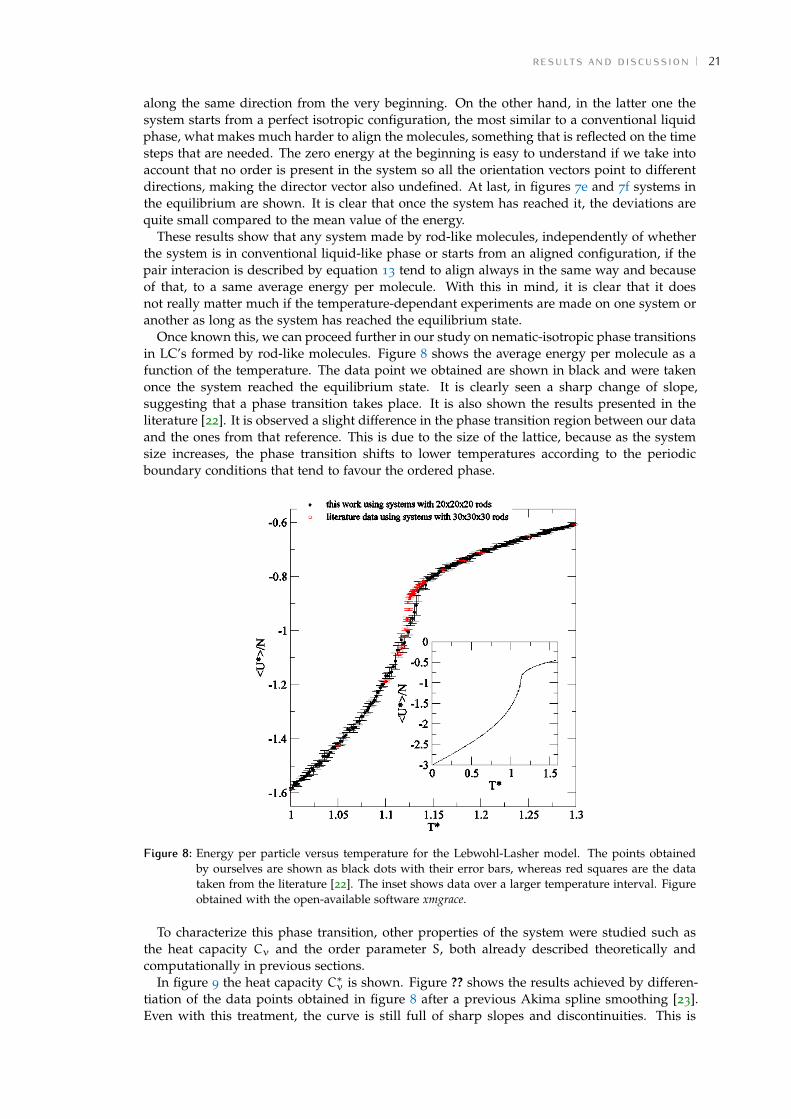
Once known this, we can proceed further in our study on nematic-isotropic phase transitionsin LC’s formed by rod-like molecules. Figure 8 shows the average energy per molecule as afunction of the temperature. The data point we obtained are shown in black and were takenonce the system reached the equilibrium state. It is clearly seen a sharp change of slope,suggesting that a phase transition takes place. It is also shown the results presented in theliterature [22]. It is observed a slight difference in the phase transition region between our dataand the ones from that reference. This is due to the size of the lattice, because as the systemsize increases, the phase transition shifts to lower temperatures according to the periodicboundary conditions that tend to favour the ordered phase.
Figure 8: Energy per particle versus temperature for the Lebwohl-Lasher model. The points obtainedby ourselves are shown as black dots with their error bars, whereas red squares are the datataken from the literature [22]. The inset shows data over a larger temperature interval. Figureobtained with the open-available software xmgrace.
To characterize this phase transition, other properties of the system were studied such asthe heat capacity Cv and the order parameter S, both already described theoretically andcomputationally in previous sections.
In figure 9 the heat capacity C∗v is shown. Figure ?? shows the results achieved by differen-
tiation of the data points obtained in figure 8 after a previous Akima spline smoothing [23].Even with this treatment, the curve is still full of sharp slopes and discontinuities. This is
conclusions and outlook 22
Figure 9: Curve of heat capacity C∗v as function of the temperature T∗ by direct differentiation of the
energy data. Figure obtained with the open-available software xmgrace.
due to the fact that it is harder to reach a good accuracy for a derivative quantity like theheat capacity. None the less,the tendency is right and the predictions are correct. The peakin the heat capacity locates the phase transition temperature at T∗ ' 1.129, according to theliterature, where this temperature is estimated to be T∗ = 1.1232± 0.0006 for a larger system.
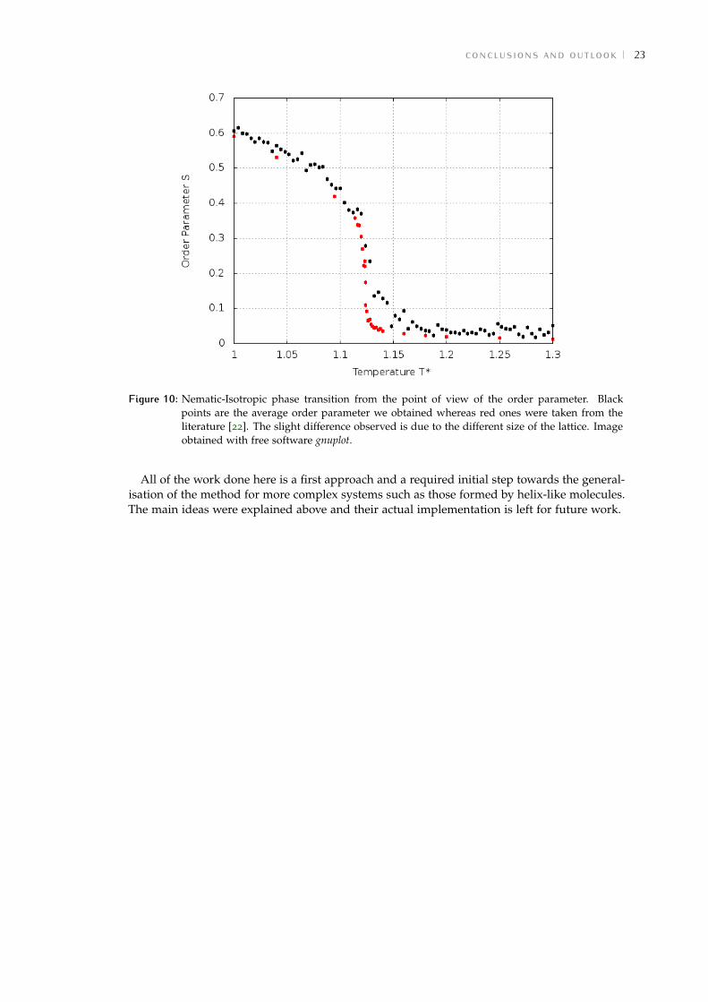
In figure 10 the average value of the order parameter is shown as function of the temperature.For every temperature the system reaches the equilibrium, and then for some large number oftime steps, the order tensorQαβ is calculated and diagonalised, whereas its biggest eigenvalueis averaged together with the ones calculated for previous time steps.
As expected, at low temperatures the order parameter is maximum, as long as the particlesare oriented better along one axis. As the temperature increases, the system undergoes a phasetransition and the order parameter decreases with a steep slope, rapidly becoming a totallydisordered system. However, order parameter’s value never reaches the zero. This is due toperiodical boundary conditions we have chosen, which do not allow the system to be fullydisorderd. That is why the reason that makes this parameter to have very small values oncethe "almost" conventional isotropic phase is reached. In other words, the non-zero value of Sis a finite system size effect.
6 conclusions and outlookWe have succesfully characterised the properties of the Lebwohl-Lasher model for LC’s. Thetransition temperature obtained, is found to be within the range suggested by the literature, ingood agreement with the results in reference [22]. The only slight difference is understood anddue to a smaller system size used that, combined with the usual periodic boundary conditions,have the effect of shifting the nematic-isotropic transition temperature to lower temperaturesas the size of the lattice increases.
According to the results obtained we can say that our code works correctly, providing quanti-tatively accurate data for the heat capacity and order parameter during the entire temperature.More simulations would be needed in order to obtain better results for the heat capacity, andlarger systems would increase the overall accuracy of the various properties.
conclusions and outlook 23
Figure 10: Nematic-Isotropic phase transition from the point of view of the order parameter. Blackpoints are the average order parameter we obtained whereas red ones were taken from theliterature [22]. The slight difference observed is due to the different size of the lattice. Imageobtained with free software gnuplot.
All of the work done here is a first approach and a required initial step towards the general-isation of the method for more complex systems such as those formed by helix-like molecules.The main ideas were explained above and their actual implementation is left for future work.
references 24
references[1] Reinitzer, F. (1888). Monatshefte für Chemie (Wien) 9 (1): 421–441
[2] Lehmann, O. (1889). Zeitschrift für Physikalische Chemie 4: 462–72.
[3] Sluckin, T. J.; Dunmur, D. A. and Stegemeyer, H. (2004). Crystals That Flow – classic papersfrom the history of liquid crystals. London: Taylor & Francis
[4] Stegemeyer, H. (1994). Professor Horst Sackmann, 1921 – 1993. Liquid Crystals Today 4: 1.
[5] Goldmacher, J. E. and Castellano, J. A. Electro-optical Compositions and Devices U.S. Patent3,540,796, Issue date: November 17, 1970.
[6] Castellano, J. A. (2005). Liquid Gold: The Story of Liquid Crystal Displays and the Creation ofan Industry. World Scientific Publishing.
[7] History and Properties of Liquid Crystals. http://www.nobelprize.org.
[8] de Gennes, P.G. & Prost, J. (1993). The Physics of Liquid Crystals, Second Edition, OxfordUniversity Press, Oxford, Great Britain.
[9] Onsanger, L. (1949). Ann. N. Y. Acad Sci. 51, 627.
[10] Flory, P.J. (1956). Proc. Roy. Soc. A234, 73.
[11] Maier W. and Saupe A. (1959). Z. Naturforsch. A 14, 882.
[12] Deloche, B., Cabane, B., and Jérôme, D. (1971). Mol. Cryst. Liquid Cryst. 15, 197.
[14] Lebwohl P. A. and Lasher G. (1972). Phys. Rev. A 6, 426.
[15] Shekhar R., Whitmer J.K., Malshe R., Moreno-Razo J.A., Roberts T. and de Pablo J.J. (2012).J. Chem. Phys. 136, 234503.
[16] Saberi A.A and Dashti-Naserabadi, H. (2011). Europhys. Lett. 92, 67005.
[17] H.B. Kolli, E. Frezza, G. Cinacchi, A. Ferrarini, G. Giacometti, T.S. Hudson. (2014). J.Chem. Phys. Communications 140, 081101; Hima Bindu Kolli, Elisa Frezza, Giorgio Cinac-chi, Alberta Ferrarini, Achille Giacometti, Toby Hudson, Cristiano De Michele, FrancescoSciortino. (2014). Soft Matter 16, 8171.
[18] Saslow, W.M., Gabay, M., Zhang, W.-M. (1992). Phys. Rev. Lett. 68, 3627.
[19] Frenkel, D. and Smit, B., Understanding Molecular Simulation, 2nd Edition (2000), AcademicPress.
[20] Metropolis,N., Rosenbluth, A.W., Rosenbluth, M.N., Teller, A., Teller, E. (1953). J. Chem.Phys. 21, 1087.
[21] Classnotes of the subject "Computación Avanzada", by Prof. Alejandro Gutiérrez duringyear 2014-2015 of the B.Sc. in Physics, Facultad de Ciencias, Universidad Autonónoma deMadrid, Madrid, Spain.
[22] Fabbri, U., Zannoni, C. (1986). Mol. Phys. 58, 763.


![The phase equilibria in the Mg–Ni–Ca systemusers.encs.concordia.ca/~mmedraj/papers/mg-ni-ca.pdf · 3. Mg–Ni System 3.1. Phase diagram Voss [ 10] was the first researcher who](https://static.documents.pub/doc/80x56/5f757c89813ca8101f07da15/the-phase-equilibria-in-the-mganiaca-mmedrajpapersmg-ni-capdf-3-mgani.jpg)


