Page 1
S TRANSFORM :
TIME FREQUENCY ANALYSIS & FILTERING
A Thesis submitted in partial fulfillment
of the requirements for the degree of
Master of Technology
in
Telematics and Signal Processing
by
NITHIN V GEORGE
ROLL NO : 207EC107
Department of Electronics and Communication Engineering
National Institute of Technology
Rourkela, India
2009
Page 2
S TRANSFORM :
TIME FREQUENCY ANALYSIS & FILTERING
A Thesis submitted in partial fulfillment
of the requirements for the degree of
Master of Technology
in
Telematics and Signal Processing
by
NITHIN V GEORGE
ROLL NO : 207EC107
under the guidance of
Dr. G. PANDA
Department of Electronics and Communication Engineering
National Institute of Technology
Rourkela, India
2009
Page 3
National Institute of Technology
Rourkela
CERTIFICATE
This is to certify that the thesis entitled, “ S Transform : Time Frequency Analysis
and Filtering ” submitted by Nithin V George in partial fulfillment of the requirements for
the award of Master of Technology Degree in Electronics & Communication Engineering
with specialization in Telematics and Signal Processing during 2008-2009 at the National
Institute of Technology, Rourkela (Deemed University) is an authentic work carried out by him
under my supervision and guidance.
To the best of my knowledge, the matter embodied in the thesis has not been submitted to
any other University / Institute for the award of any Degree or Diploma.
Date Prof. G. Panda (FNAE, FNASc)
Dept. of Electronics & Communication Engg.
National Institute of Technology
Rourkela-769008
Orissa, India
Page 4
Acknowledgements
I am deeply indebted to Dr. G. Panda, my supervisor on this project, for consistently
providing me with the required guidance to help me in the timely and successful comple-
tion of this project. In spite of his extremely busy schedules, he was always available to
share with me his deep insights, wide knowledge and extensive experience. His advices
have value lasting much beyond this project. I consider it a blessing to be associated
with him.
The completion of the research work that culminates into this thesis wouldn’t have
been possible without the able guidance of Dr. Lalu Mansinha of the University of
Western Ontario, London, Canada. I consider myself highly fortunate to have received
the opportunity to learn from this erudite and equanimous teacher. Although he was
not part of the UWO faculty, he had spared substantial amount of his personal time for
me and gave me the required inputs, advices and assistance. I would like to gratefully
acknowledge all his support and guidance.
I also owe many thanks to Dr. Kristy F Tiampo of the University of Western
Ontario, London, Canada who had supervised my project work at UWO. The energy
and effectiveness inherent in all her involvement had been amazing. I would consider
her a role model for anyone aspiring to be successful in life. I am also grateful to the
University of Western Ontario, London, Canada for granting me the required access to
the resources available at the department of Earth Sciences.
I was also the beneficiary of essential advice and assistance of the faculty and staff
at NIT Rourkela. I gratefully acknowledge the kindness and cooperation extended to
me specially by Dr.S.K.Patra (Head, Department of Electronics and Communication
Engineering), Dr.G.S.Rath, Dr.K.K.Mahapatra, Dr.S.Meher, Dr.S.K.Behera ,
Dr.D.P.Acharya and Prof.A.K.Sahoo . I also remember with gratitude my friends
who have been always available at hand to motivate, encourage and help me out.
Finally I would like to thank the Department of Foreign Affairs and International
Trade (DFAIT), Govt. of Canada, for the scholarship granted to me that had provided
me the financial support to successfully complete my assignments under the Graduate
Student Exchange Programme (GSEP) fellowship at the University of Western Ontario,
London, Canada.
Nithin V George
Page 5
Contents
Contents i
Abstract iv
List of Figures v
List of Tables vii
List of Acronyms viii
1 Introduction 1
2 Time Series Analysis 4
2.1 Introduction . . . . . . . . . . . . . . . . . . . . . . . . . . . . . . . . . . 5
2.2 Trend Analysis . . . . . . . . . . . . . . . . . . . . . . . . . . . . . . . . 6
2.3 Seasonality Analysis . . . . . . . . . . . . . . . . . . . . . . . . . . . . . 6
2.4 Spectral Analysis . . . . . . . . . . . . . . . . . . . . . . . . . . . . . . . 7
2.4.1 Fourier Transform . . . . . . . . . . . . . . . . . . . . . . . . . . . 7
2.4.2 Short Time Fourier Transform(STFT) . . . . . . . . . . . . . . . 9
2.4.3 The Wavelet Transform . . . . . . . . . . . . . . . . . . . . . . . 12
2.5 Discussion . . . . . . . . . . . . . . . . . . . . . . . . . . . . . . . . . . . 14
3 Modified S Transform 15
3.1 Introduction . . . . . . . . . . . . . . . . . . . . . . . . . . . . . . . . . . 16
3.2 Stockwell Transform . . . . . . . . . . . . . . . . . . . . . . . . . . . . . 16
3.3 Comparison of S Transform and CWT . . . . . . . . . . . . . . . . . . . 19
3.4 Generalized S Transform . . . . . . . . . . . . . . . . . . . . . . . . . . . 21
3.5 Modified S Transform . . . . . . . . . . . . . . . . . . . . . . . . . . . . . 22
3.6 Simulation and Discussion . . . . . . . . . . . . . . . . . . . . . . . . . . 25
3.6.1 Example 1 . . . . . . . . . . . . . . . . . . . . . . . . . . . . . . . 25
3.6.2 Example 2 . . . . . . . . . . . . . . . . . . . . . . . . . . . . . . . 25
3.7 Conclusion . . . . . . . . . . . . . . . . . . . . . . . . . . . . . . . . . . . 27
Page 6
CONTENTS
4 Analysis of Business Cycles 28
4.1 Introduction . . . . . . . . . . . . . . . . . . . . . . . . . . . . . . . . . . 29
4.2 Causes of Business cycles . . . . . . . . . . . . . . . . . . . . . . . . . . . 29
4.3 Economic Indicators . . . . . . . . . . . . . . . . . . . . . . . . . . . . . 30
4.4 Types of business cycles . . . . . . . . . . . . . . . . . . . . . . . . . . . 31
4.4.1 Kondratiev cycles . . . . . . . . . . . . . . . . . . . . . . . . . . . 32
4.5 Analysis and Discussion . . . . . . . . . . . . . . . . . . . . . . . . . . . 34
4.6 Conclusion . . . . . . . . . . . . . . . . . . . . . . . . . . . . . . . . . . . 39
5 Time Frequency Filtering
- An Alternate Approach 40
5.1 Introduction . . . . . . . . . . . . . . . . . . . . . . . . . . . . . . . . . . 41
5.2 Literature Survey . . . . . . . . . . . . . . . . . . . . . . . . . . . . . . . 42
5.3 The Proposed Filtering Approach . . . . . . . . . . . . . . . . . . . . . . 44
5.3.1 Background Noise Removal . . . . . . . . . . . . . . . . . . . . . 44
5.3.2 Localised Noise Filtering . . . . . . . . . . . . . . . . . . . . . . . 44
5.4 Simulation and Discussions . . . . . . . . . . . . . . . . . . . . . . . . . . 46
5.4.1 Example 1 . . . . . . . . . . . . . . . . . . . . . . . . . . . . . . . 46
5.4.2 Example 2 . . . . . . . . . . . . . . . . . . . . . . . . . . . . . . . 49
5.5 Conclusion . . . . . . . . . . . . . . . . . . . . . . . . . . . . . . . . . . . 53
6 Application to Geophysics 54
6.1 Introduction . . . . . . . . . . . . . . . . . . . . . . . . . . . . . . . . . . 55
6.2 Basic Concept of GPS . . . . . . . . . . . . . . . . . . . . . . . . . . . . 55
6.2.1 Space segment . . . . . . . . . . . . . . . . . . . . . . . . . . . . . 56
6.2.2 Control segment . . . . . . . . . . . . . . . . . . . . . . . . . . . . 56
6.2.3 User Segment . . . . . . . . . . . . . . . . . . . . . . . . . . . . . 57
6.3 The Structure of the GPS signal . . . . . . . . . . . . . . . . . . . . . . . 57
6.3.1 Modulation of the carrier signals . . . . . . . . . . . . . . . . . . 57
6.4 Errors in GPS . . . . . . . . . . . . . . . . . . . . . . . . . . . . . . . . . 58
6.4.1 Satellite Geometry . . . . . . . . . . . . . . . . . . . . . . . . . . 58
6.4.2 Satellite Orbits . . . . . . . . . . . . . . . . . . . . . . . . . . . . 59
6.4.3 Multipath Effect . . . . . . . . . . . . . . . . . . . . . . . . . . . 59
6.4.4 Atmospheric effects . . . . . . . . . . . . . . . . . . . . . . . . . . 59
6.4.5 Relativistic effects . . . . . . . . . . . . . . . . . . . . . . . . . . . 60
6.5 Literature Survey . . . . . . . . . . . . . . . . . . . . . . . . . . . . . . . 60
ii
Page 7
CONTENTS
6.5.1 Glacial Isostatic Adjustment (GIA) . . . . . . . . . . . . . . . . . 61
6.6 Region of Study . . . . . . . . . . . . . . . . . . . . . . . . . . . . . . . . 61
6.7 S Transform Filtering . . . . . . . . . . . . . . . . . . . . . . . . . . . . . 63
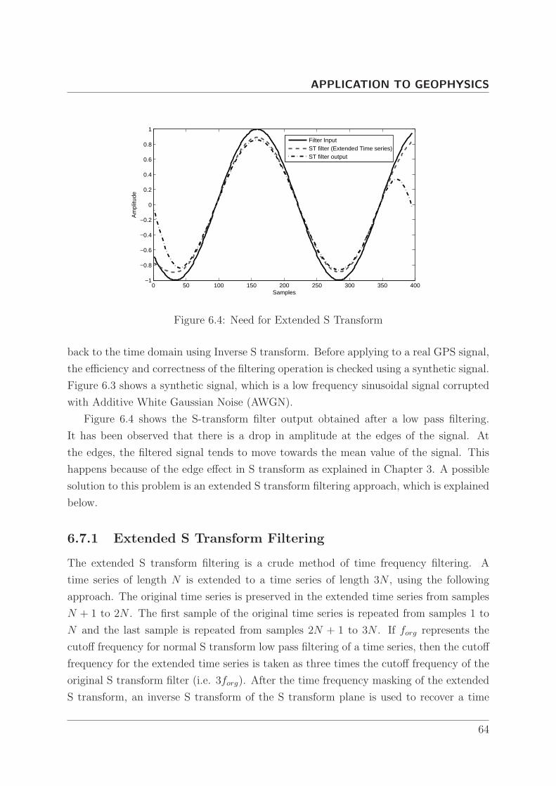
6.7.1 Extended S Transform Filtering . . . . . . . . . . . . . . . . . . . 64
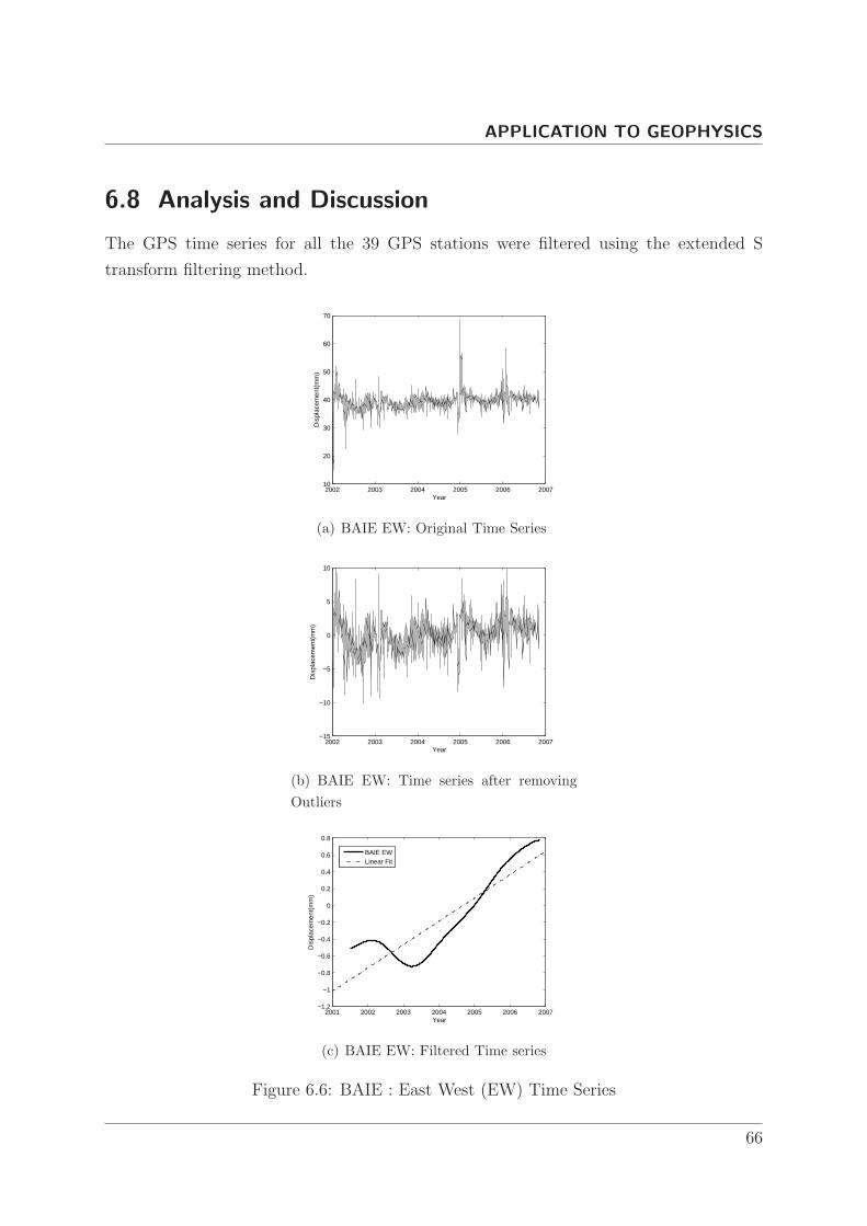
6.8 Analysis and Discussion . . . . . . . . . . . . . . . . . . . . . . . . . . . 66
6.9 Conclusion . . . . . . . . . . . . . . . . . . . . . . . . . . . . . . . . . . . 72
7 Concluding Remarks 73
7.1 Conclusion . . . . . . . . . . . . . . . . . . . . . . . . . . . . . . . . . . . 74
7.2 Scope for Future Work . . . . . . . . . . . . . . . . . . . . . . . . . . . . 74
Bibliography 76
iii
Page 8
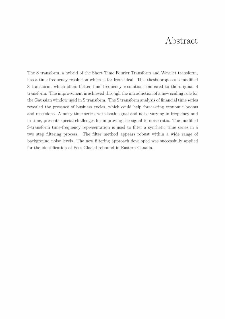
Abstract
The S transform, a hybrid of the Short Time Fourier Transform and Wavelet transform,
has a time frequency resolution which is far from ideal. This thesis proposes a modified
S transform, which offers better time frequency resolution compared to the original S
transform. The improvement is achieved through the introduction of a new scaling rule for
the Gaussian window used in S transform. The S transform analysis of financial time series
revealed the presence of business cycles, which could help forecasting economic booms
and recessions. A noisy time series, with both signal and noise varying in frequency and
in time, presents special challenges for improving the signal to noise ratio. The modified
S-transform time-frequency representation is used to filter a synthetic time series in a
two step filtering process. The filter method appears robust within a wide range of
background noise levels. The new filtering approach developed was successfully applied
for the identification of Post Glacial rebound in Eastern Canada.
Page 9
List of Figures
2.1 Series ‘G’ . . . . . . . . . . . . . . . . . . . . . . . . . . . . . . . . . . . 5
2.2 Fourier Amplitude Spectrum : Fractional Frequencies . . . . . . . . . . . 8
2.3 Fourier Amplitude Spectrum : Stationary Signal . . . . . . . . . . . . . . 9
2.4 Fourier Amplitude Spectrum : Non Stationary Signal . . . . . . . . . . . 10
2.5 Amplitude Spectrum of a 4Hz sinusoidal signal of 1000 samples with a
40Hz signal for a short duration of 30 samples . . . . . . . . . . . . . . . 11
2.6 Short Time Fourier Transform . . . . . . . . . . . . . . . . . . . . . . . . 12
2.7 Mexican Hat Wavelet . . . . . . . . . . . . . . . . . . . . . . . . . . . . . 13
2.8 The Wavelet Transform . . . . . . . . . . . . . . . . . . . . . . . . . . . . 14
3.1 S Transform TFR of test time series . . . . . . . . . . . . . . . . . . . . . 20
3.2 Scaling function γ . . . . . . . . . . . . . . . . . . . . . . . . . . . . . . . 22
3.3 Variation of window width with γ for a particular frequency(25Hz) . . . 23
3.4 Example 1 - TFR Using S Transform and Modified S Transform . . . . . 24
3.5 Example 2 - TFR Using S Transform and Modified S Transform . . . . . 26
4.1 Monthly Average Closing Price - DJIA . . . . . . . . . . . . . . . . . . . 33
4.2 Monthly Average Closing Price - S&P 500 . . . . . . . . . . . . . . . . . 34
4.3 S Transform - DJIA . . . . . . . . . . . . . . . . . . . . . . . . . . . . . . 35
4.4 S Transform - SNP . . . . . . . . . . . . . . . . . . . . . . . . . . . . . . 35
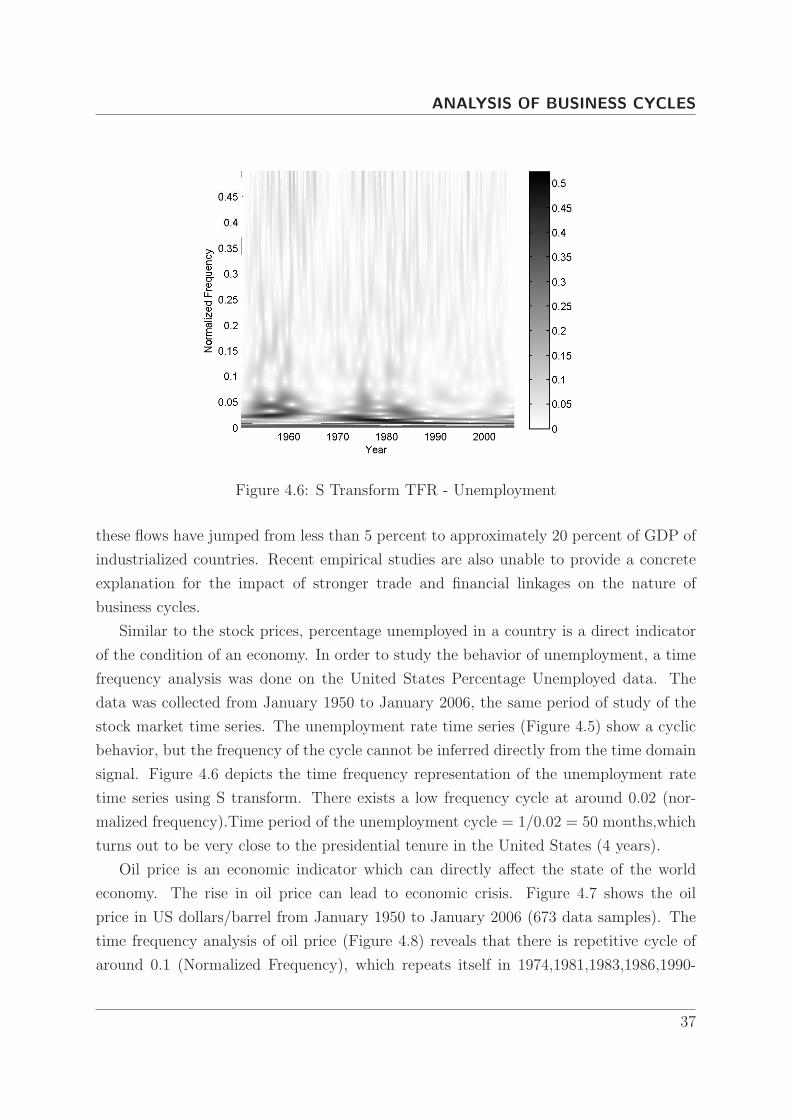
4.5 Percentage Unemployed (U.S) . . . . . . . . . . . . . . . . . . . . . . . . 36
4.6 S Transform TFR - Unemployment . . . . . . . . . . . . . . . . . . . . . 37
4.7 Oil Price (US Dollars/barrel) . . . . . . . . . . . . . . . . . . . . . . . . 38
4.8 S Transform TFR - Oil Price . . . . . . . . . . . . . . . . . . . . . . . . . 38
5.1 Need for LTV filters . . . . . . . . . . . . . . . . . . . . . . . . . . . . . 42
5.2 Example 1 - Input Signal . . . . . . . . . . . . . . . . . . . . . . . . . . . 45
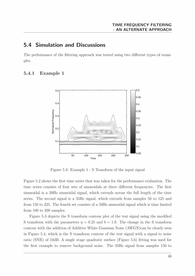
5.3 Example 1 - S Transform of the input signal . . . . . . . . . . . . . . . . 46
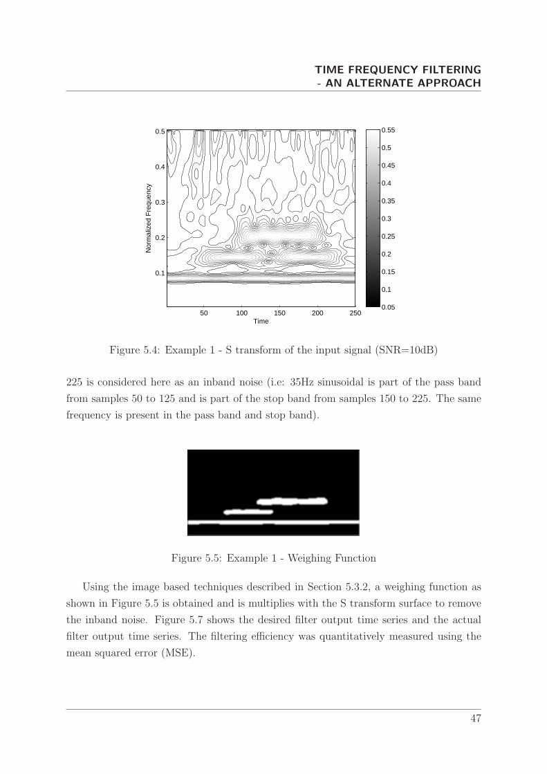
5.4 Example 1 - S transform of the input signal (SNR=10dB) . . . . . . . . . 47
5.5 Example 1 - Weighing Function . . . . . . . . . . . . . . . . . . . . . . . 47
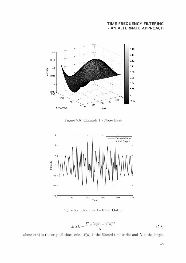
5.6 Example 1 - Noise Base . . . . . . . . . . . . . . . . . . . . . . . . . . . 48
5.7 Example 1 - Filter Output . . . . . . . . . . . . . . . . . . . . . . . . . . 48
Page 10
LIST OF FIGURES
5.8 Example 2 - Input Signal . . . . . . . . . . . . . . . . . . . . . . . . . . . 49
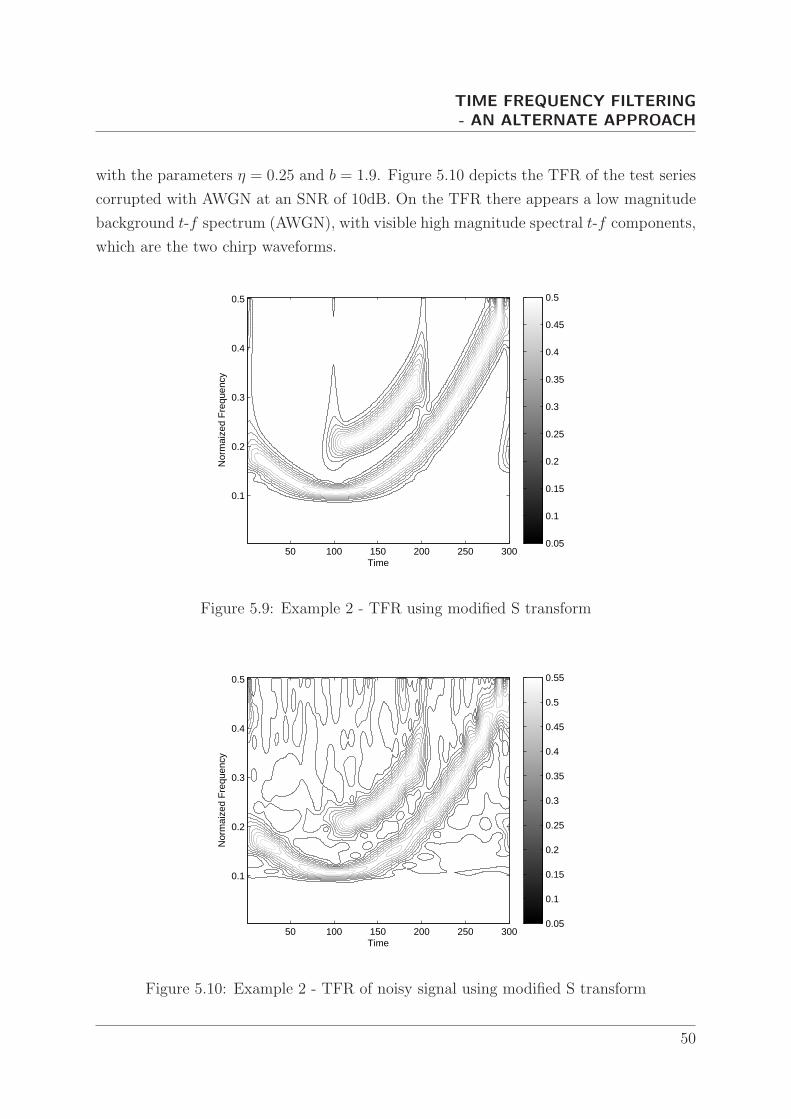
5.9 Example 2 - TFR using modified S transform . . . . . . . . . . . . . . . 50
5.10 Example 2 - TFR of noisy signal using modified S transform . . . . . . . 50
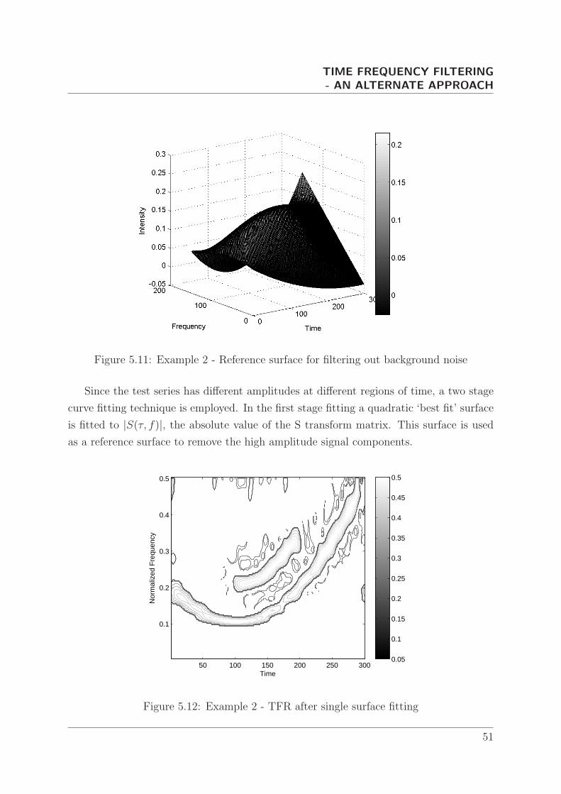
5.11 Example 2 - Reference surface for filtering out background noise . . . . . 51
5.12 Example 2 - TFR after single surface fitting . . . . . . . . . . . . . . . . 51
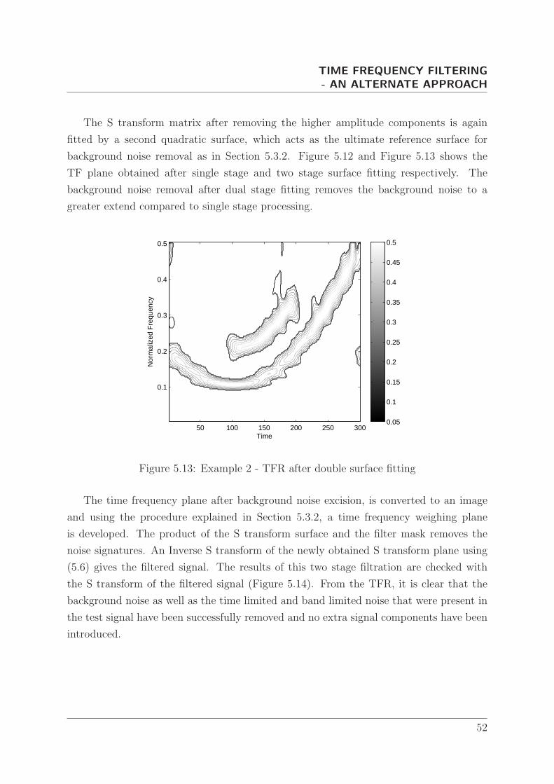
5.13 Example 2 - TFR after double surface fitting . . . . . . . . . . . . . . . . 52
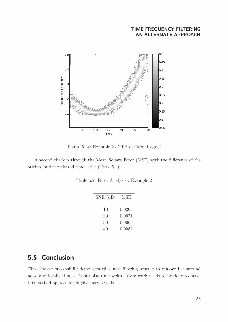
5.14 Example 2 - TFR of filtered signal . . . . . . . . . . . . . . . . . . . . . 53
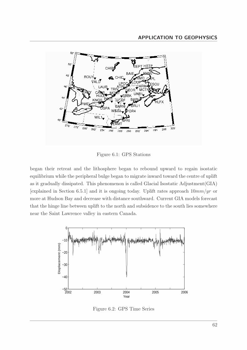
6.1 GPS Stations . . . . . . . . . . . . . . . . . . . . . . . . . . . . . . . . . 62
6.2 GPS Time Series . . . . . . . . . . . . . . . . . . . . . . . . . . . . . . . 62
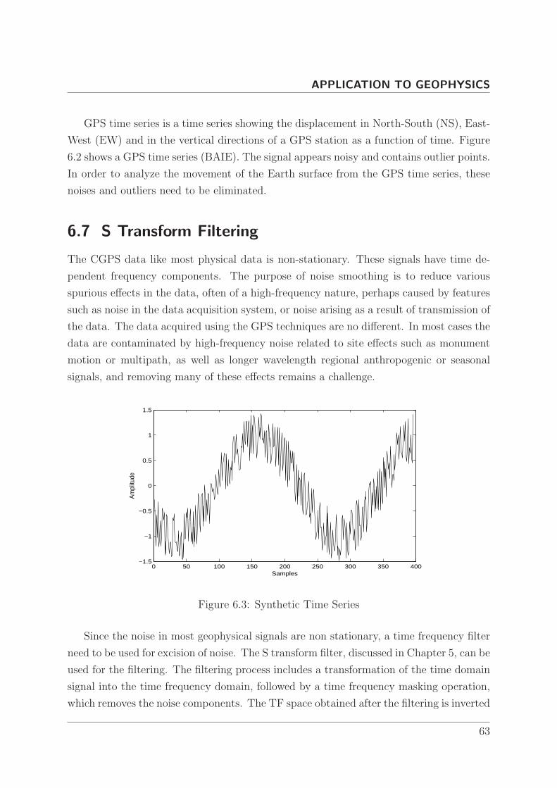
6.3 Synthetic Time Series . . . . . . . . . . . . . . . . . . . . . . . . . . . . . 63
6.4 Need for Extended S Transform . . . . . . . . . . . . . . . . . . . . . . . 64
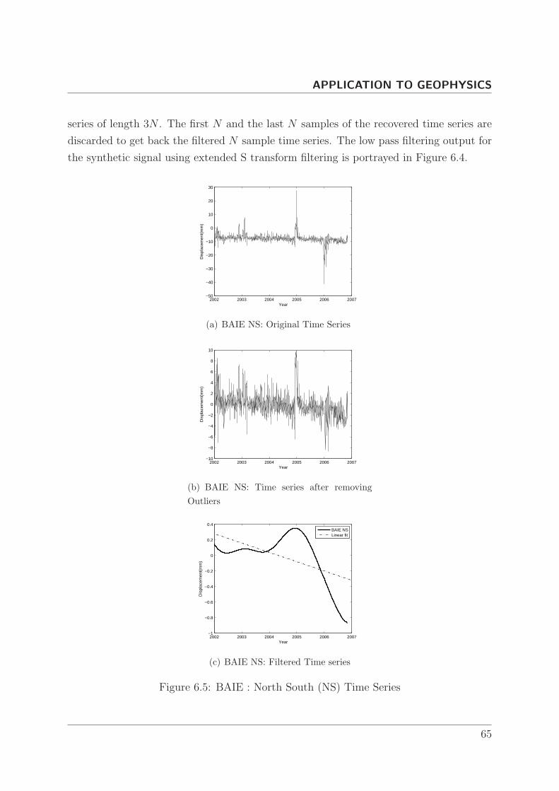
6.5 BAIE : North South (NS) Time Series . . . . . . . . . . . . . . . . . . . 65
6.6 BAIE : East West (EW) Time Series . . . . . . . . . . . . . . . . . . . . 66
6.7 BAIE : Vertical Time Series . . . . . . . . . . . . . . . . . . . . . . . . . 67
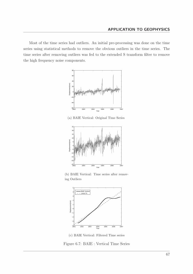
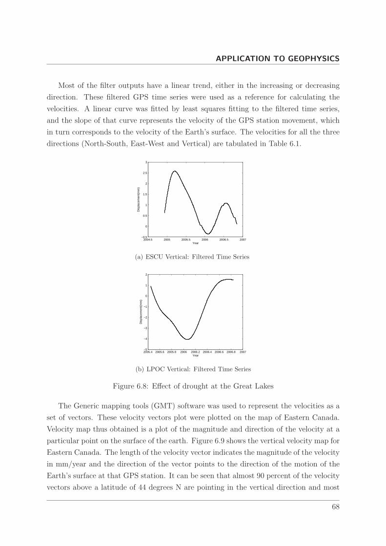
6.8 Effect of drought at the Great Lakes . . . . . . . . . . . . . . . . . . . . 68
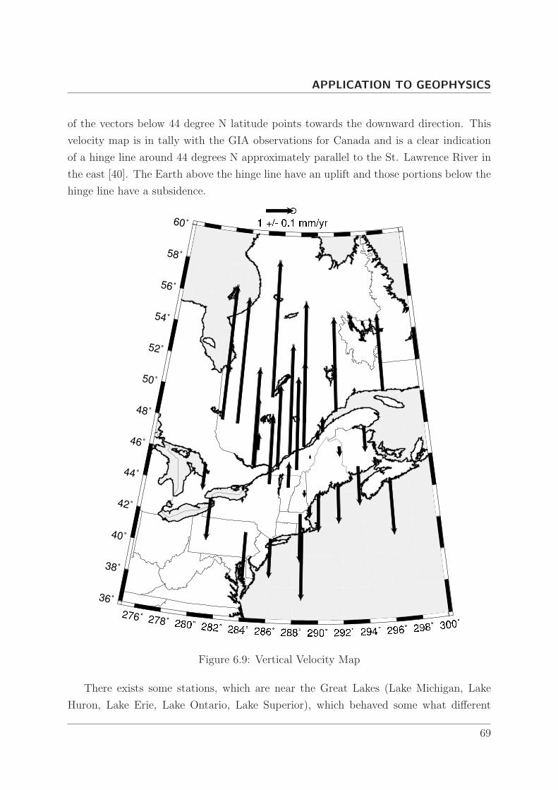
6.9 Vertical Velocity Map . . . . . . . . . . . . . . . . . . . . . . . . . . . . . 69
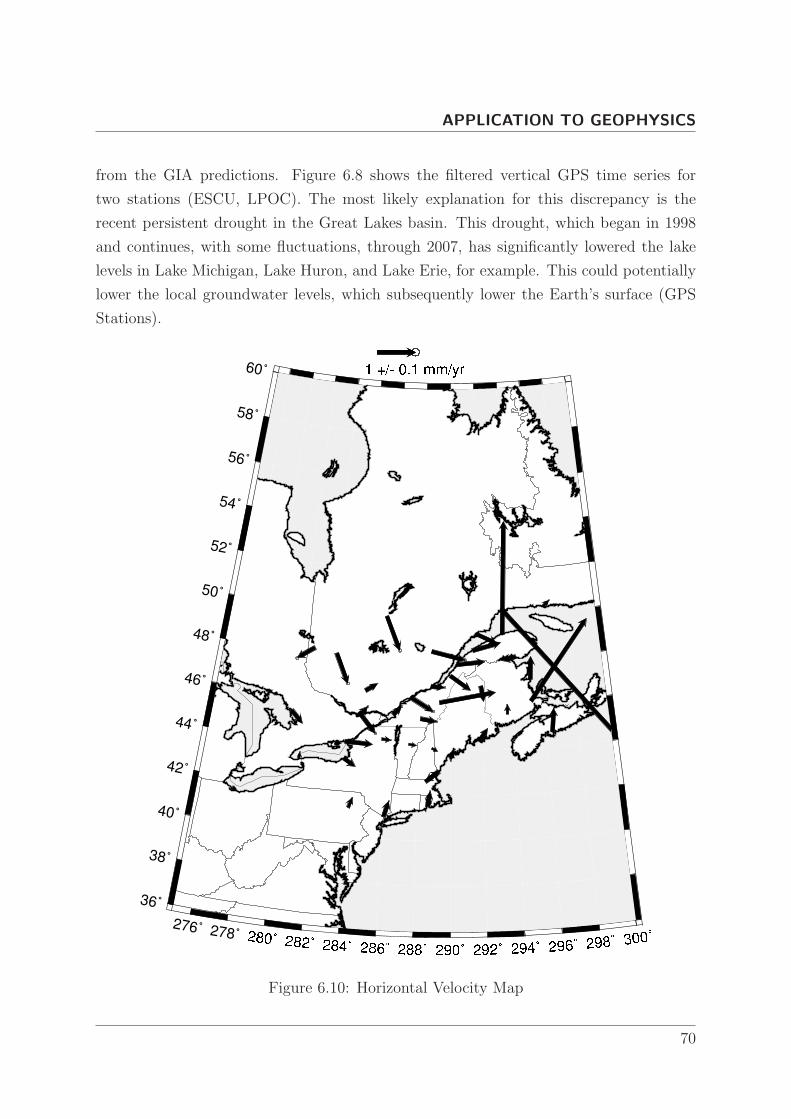
6.10 Horizontal Velocity Map . . . . . . . . . . . . . . . . . . . . . . . . . . . 70
vi
Page 11
List of Tables
4.1 Oil Price Peaks . . . . . . . . . . . . . . . . . . . . . . . . . . . . . . . . 39
5.1 Error Analysis : Example 1 . . . . . . . . . . . . . . . . . . . . . . . . . 49
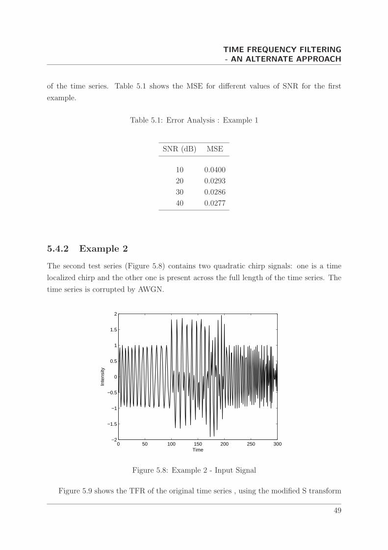
5.2 Error Analysis : Example 2 . . . . . . . . . . . . . . . . . . . . . . . . . 53
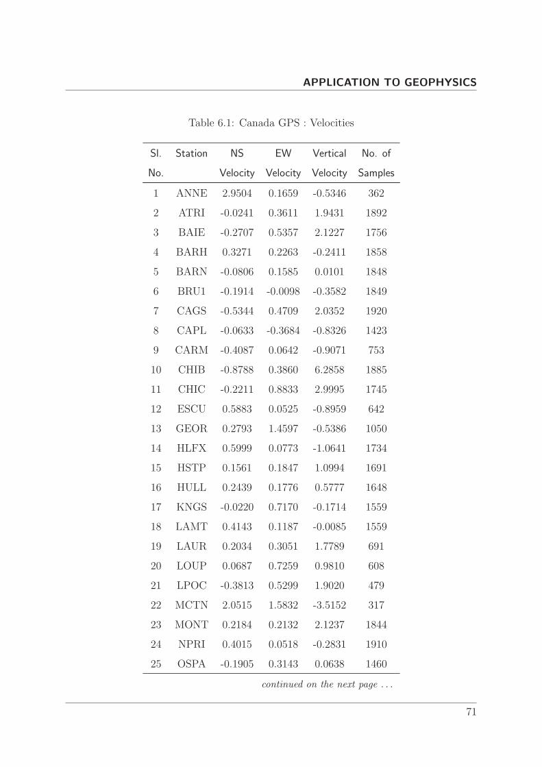
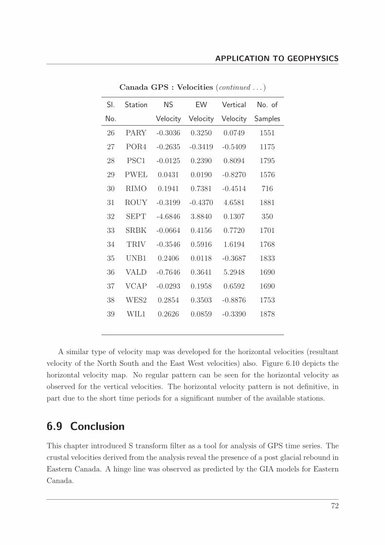
6.1 Canada GPS : Velocities . . . . . . . . . . . . . . . . . . . . . . . . . . . 71
Page 12
List of Acronyms
FT Fourier Transform
STFT Short Time Fourier Transform
WT Wavelet Transform
CWT Continuous Wavelet Transform
DWT Discrete Wavelet Transform
TFR Time Frequency Representation
LTV Linear Time Varying
ST Stockwell Transform
GDP Gross Domestic Product
GPS Global Positioning System
NS North South
EW East West
GIA Glacial Isostatic Adjustment
GMT Generic Mapping Tools
TV Time Variance
Page 14
INTRODUCTION
A time series is a sequence of data points, measured typically at successive times. A
time series x(t) , t = 1, 2, . . . is called a stationary time series if its statistical properties
do not change with time t. Spectral Analysis using the Fourier transform is a powerful
tool for stationary time series analysis. But for non-stationary time series, the statistical
properties changes with time and hence the time averaged amplitude spectrum obtained
using Fourier transform is inadequate to track the changes in the signal magnitude,
frequency or phase. The advent of time frequency analysis techniques using Short Time
Fourier Transform (STFT) and Wavelet Transform made the analysis of non stationary
signals simpler. The fixed resolution of the STFT and the absence of phase information
in the Wavelet transform led to the development of the S transform, which retains the
absolute phase information, in the mean while, have good time frequency resolution for all
frequencies. Even though the S transform has better time frequency resolution compared
to STFT, the resolution if far from ideal. The resolution needs improvement.
Integrating the S transform over time results in the Fourier transform. This direct
relation to the Fourier transform makes the inversion to time domain an easy task. This
property of the S transform led to the development of S transform filters, which uses an
analysis-weighting-synthesis procedure. The extra time dimension in the time frequency
filters gives the designer an enhanced opportunity to clearly define the pass bands and stop
bands. Current literature on time frequency filters using S transform uses a regular shaped
pass band or stop band (e.g. Rectangular), which makes the filtering intricate when
the signal and the noise exists in an irregular intermixed pattern in the time frequency
domain.
The objective of this work is to improve the time frequency resolution of S transform,
develop a simple in-band filtering approach using S transform and to use the filtering
technique for analysis of Geophysical time series. The thesis is organized as follows.
Chapter 2 gives an introduction to time series analysis. It also includes a brief review
of the signal processing tools like the Fourier transform, Short Time Fourier transform and
the Wavelet transform. The short comparison between the advantages and disadvantages
of each method is presented.
Chapter 3 presents the S transform, which is a new time frequency analysis technique.
A modified S transform is proposed , which has better time frequency resolution compared
to the original S transform. The improvement in resolution is demonstrated using a set
of synthetic time series.
In Chapter 4, the S transform is used for the analysis of Business cycles. Stock price
indices are used as an indicator of the business cycles. Valuable information that are
2
Page 15
INTRODUCTION
obvious neither from the time series nor from the Fourier analysis of business data are
obtained using S transform time frequency analysis.
A novel time frequency filtering approach is introduced in Chapter 5. Image process-
ing algorithms are combined with S transform to perform filtering of noisy time series,
with both signal and noise varying in frequency and in time. The filtering procedure is
validated using synthetic signals.
The time frequency filtering procedure introduced in Chapter 5, is applied to real data
in Chapter 6. In Chapter 6, time frequency filters are applied to filter Global Positioning
System (GPS) time series collected for Eastern Canada. The study reveals the presence
of a post glacial rebound. The results are in close match with the Post Glacial Rebound
models for Eastern Canada.
Conclusions are drawn in Chapter 7. Future work has also been discussed in this
chapter.
3
Page 16
2Time Series Analysis
Page 17
TIME SERIES ANALYSIS
2.1 Introduction
A time-series is a set of data recorded over a length of time. It is normally an output
of a measuring instrument. Most time series patterns can be described in terms of two
basic classes of components: trend and seasonality. Trend is a general systematic linear
or nonlinear component that changes over time and does not repeat or at least does not
repeat within the time range of the time series. Seasonality is similar to trend but it
repeats itself in systematic intervals over time. These two general classes of time series
components may coexist in real-life data.
Jan 1949 Dec 19600
100
200
300
400
500
600
700
Month
Inte
rnat
iona
l Airl
ine
Pas
seng
ers
(Tho
usan
ds)
DataLinear Trend
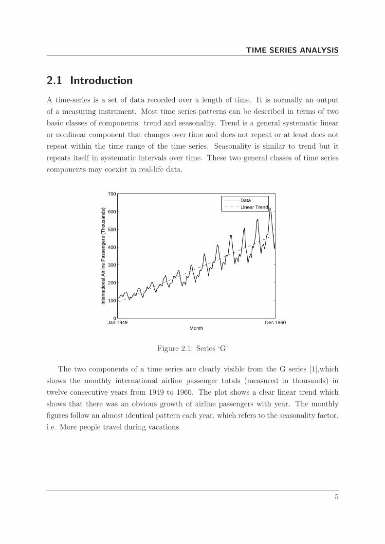
Figure 2.1: Series ‘G’
The two components of a time series are clearly visible from the G series [1],which
shows the monthly international airline passenger totals (measured in thousands) in
twelve consecutive years from 1949 to 1960. The plot shows a clear linear trend which
shows that there was an obvious growth of airline passengers with year. The monthly
figures follow an almost identical pattern each year, which refers to the seasonality factor.
i.e. More people travel during vacations.
5
Page 18
TIME SERIES ANALYSIS
2.2 Trend Analysis
There is no well laid out rule or technique to calculate trend in a time series. If the trend is
either a monotonically increasing or decreasing one, its computation may not be difficult.
If the time series data contain considerable error, then the first step in the process of
trend identification is smoothing. Smoothing normally involves a form of local averaging
of data such that the non systematic components of simultaneous observations cancel each
other out. The most common technique is moving average smoothing which replaces each
element of the series by either the simple or weighted average of N surrounding elements,
where N is the width of the smoothing ‘window’ [1]. Medians can be used instead of
means. The main advantage of median as compared to moving average smoothing is that
its results are less biased by outliers (within the smoothing window). Thus, if there are
outliers in the data, median smoothing typically produces smoother curves than moving
average based on the same window width. The main disadvantage of median smoothing
is that in the absence of clear outliers it may produce more ‘jagged’ curves than moving
average and it does not allow for weighting. A normal trend identification involves a
lower order polynomial, exponential or logarithmic curve fitting to the time series after
removing non linear components by smoothing.
2.3 Seasonality Analysis
Seasonality is defined as correlational dependency of order k between each ith element
of the series and the (i− k)th element and measured by autocorrelation. The parameter
k is usually called the lag. If the time series is devoid of outliers and large measurement
errors, seasonality can be visually identified in the series as a pattern that repeats every
k elements. The seasonality of a time series can be analyzed using a correlogram, which
displays graphically and numerically the autocorrelation function , that is, serial correla-
tion coefficients for consecutive lags in a specified range of lags. Serial dependency for a
particular lag of k can be removed by differencing the series, that is converting each ith
element of the series into its difference from the (i− k)th element. There are two major
reasons for such transformations. First, one can identify the hidden nature of seasonal
dependencies in the series. The second reason for removing serial dependency is to make
the time series stationary (constant mean, variance, and autocorrelation through out the
full length of the time series).
6
Page 19
TIME SERIES ANALYSIS
2.4 Spectral Analysis
Spectral Analysis is a third type of analysis that can be done on a time series. It is used
to study the cyclic nature of a time series apart from the seasonality.
2.4.1 Fourier Transform
Fourier Transform is one of most common spectral analysis technique. It transforms a
time domain signal to a frequency domain signal, which is an alternate representation of
a signal. In most cases the frequency domain shows certain features of the signal that
were not visible in the time domain. Fourier transform changes the delta basis function
in the time domain to infinitely long sinusoidal basis functions in the frequency domain.
The sinusoidal basis functions are the solutions to the mathematical equation describing
a small perturbation of a physical system about a stable equilibrium point [2].
The Fourier transform X(f) of a time series x(t) is given by
X(f) =
∫∞
−∞
x(t)e−i2πftdt (2.1)
and its inverse relationship is given by
x(t) =
∫∞
−∞
X(f)ei2πftdf (2.2)
The discrete version of the Fourier Transform called the Discrete Fourier Transform
(DFT) of a time series of length N is given by
X[ n
NT
]=
1
N
N−1∑
k=0
x(kT )e−( i2πnkN ) (2.3)
where T is the sampling interval of the time series. The inversion relationship is
x(kT ) =N−1∑
n=0
X[ n
NT
]e(
i2πnkN ) (2.4)
Study of the function [X(f)]2 is called Periodogram Analysis. Even though Fourier
transform can estimate all integer frequencies to a certain extend, it has several disad-
vantages :
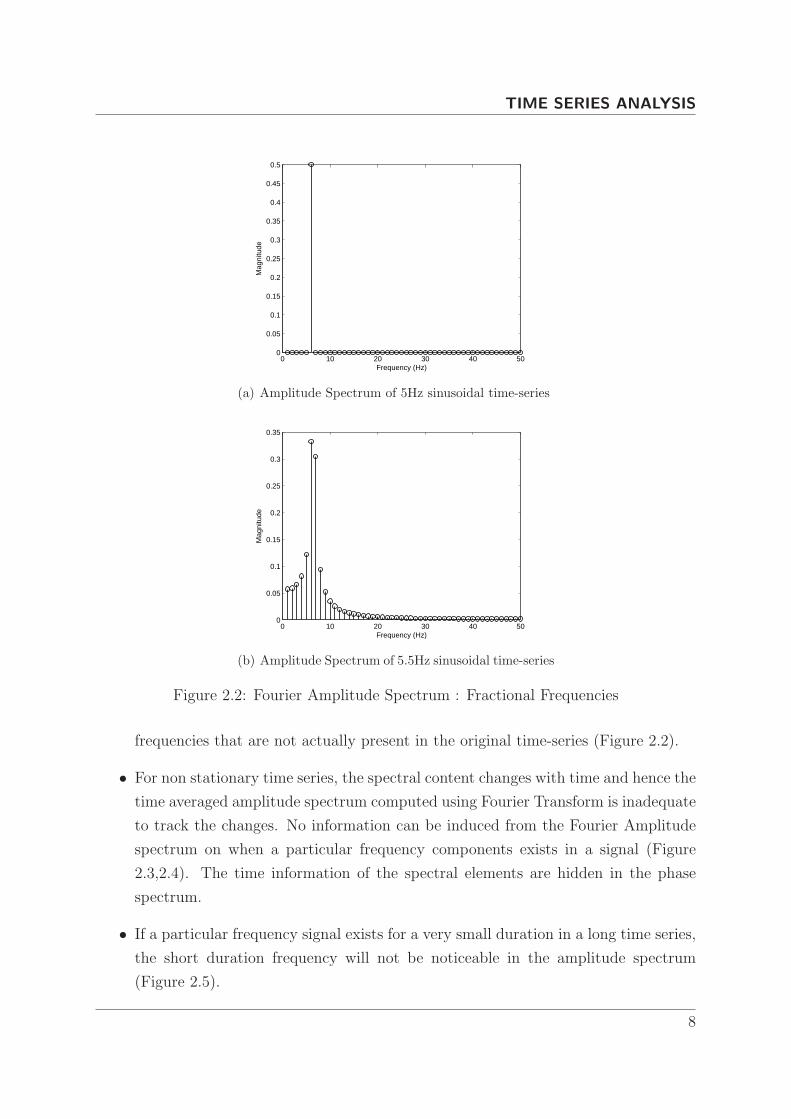
• Fourier Transform cannot estimate fractional frequencies. The Fourier Transform
of signals with fractional frequencies, results in spreading of the spectrum to other
7
Page 20
TIME SERIES ANALYSIS
0 10 20 30 40 500
0.05
0.1
0.15
0.2
0.25
0.3
0.35
0.4
0.45
0.5
Frequency (Hz)
Mag
nitu
de
(a) Amplitude Spectrum of 5Hz sinusoidal time-series
0 10 20 30 40 500
0.05
0.1
0.15
0.2
0.25
0.3
0.35
Frequency (Hz)
Mag
nitu
de
(b) Amplitude Spectrum of 5.5Hz sinusoidal time-series
Figure 2.2: Fourier Amplitude Spectrum : Fractional Frequencies
frequencies that are not actually present in the original time-series (Figure 2.2).
• For non stationary time series, the spectral content changes with time and hence the
time averaged amplitude spectrum computed using Fourier Transform is inadequate
to track the changes. No information can be induced from the Fourier Amplitude
spectrum on when a particular frequency components exists in a signal (Figure
2.3,2.4). The time information of the spectral elements are hidden in the phase
spectrum.
• If a particular frequency signal exists for a very small duration in a long time series,
the short duration frequency will not be noticeable in the amplitude spectrum
(Figure 2.5).
8
Page 21
TIME SERIES ANALYSIS
0 200 400 600 800 1000−2
−1.5
−1
−0.5
0
0.5
1
1.5
2
Time
Mag
nitu
de
(a) A 4Hz sinusoidal time-series added with an 8Hz si-nusoidal time-series
0 10 20 30 40 500
0.05
0.1
0.15
0.2
0.25
0.3
0.35
0.4
0.45
0.5
Frequency (Hz)
Mag
nitu
de
(b) Amplitude Spectrum of the above time series
Figure 2.3: Fourier Amplitude Spectrum : Stationary Signal
The solution to most of the above mentioned difficulties of Fourier Transform is the
Time-Frequency spectral analysis.
2.4.2 Short Time Fourier Transform(STFT)
STFT was one of the first Time-Frequency representation technique. It multiplies the
time series with a series of shifted time windows and calculates the Fourier transform of
that multiplied signal [3]. STFT of a signal x(t) is given by:
STFT (τ, f) =
∫∞
−∞
x(t)w(t− τ)e−i2πftdt (2.5)
9
Page 22
TIME SERIES ANALYSIS
0 200 400 600 800 1000−1
−0.8
−0.6
−0.4
−0.2
0
0.2
0.4
0.6
0.8
1
Time
Mag
nitu
de
(a) Time series with 4Hz sinusoidal for first 500 samplesand with an 8Hz sinusoidal for the next 500 samples
0 10 20 30 40 500
0.05
0.1
0.15
0.2
0.25
Frequency (Hz)
Mag
nitu
de
(b) Amplitude Spectrum of the above time series
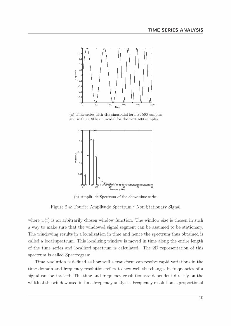
Figure 2.4: Fourier Amplitude Spectrum : Non Stationary Signal
where w(t) is an arbitrarily chosen window function. The window size is chosen in such
a way to make sure that the windowed signal segment can be assumed to be stationary.
The windowing results in a localization in time and hence the spectrum thus obtained is
called a local spectrum. This localizing window is moved in time along the entire length
of the time series and localized spectrum is calculated. The 2D representation of this
spectrum is called Spectrogram.
Time resolution is defined as how well a transform can resolve rapid variations in the
time domain and frequency resolution refers to how well the changes in frequencies of a
signal can be tracked. The time and frequency resolution are dependent directly on the
width of the window used in time frequency analysis. Frequency resolution is proportional
10
Page 23
TIME SERIES ANALYSIS
0 10 20 30 40 500
0.05
0.1
0.15
0.2
0.25
0.3
0.35
0.4
0.45
0.5
Frequency (Hz)
Mag
nitu
de
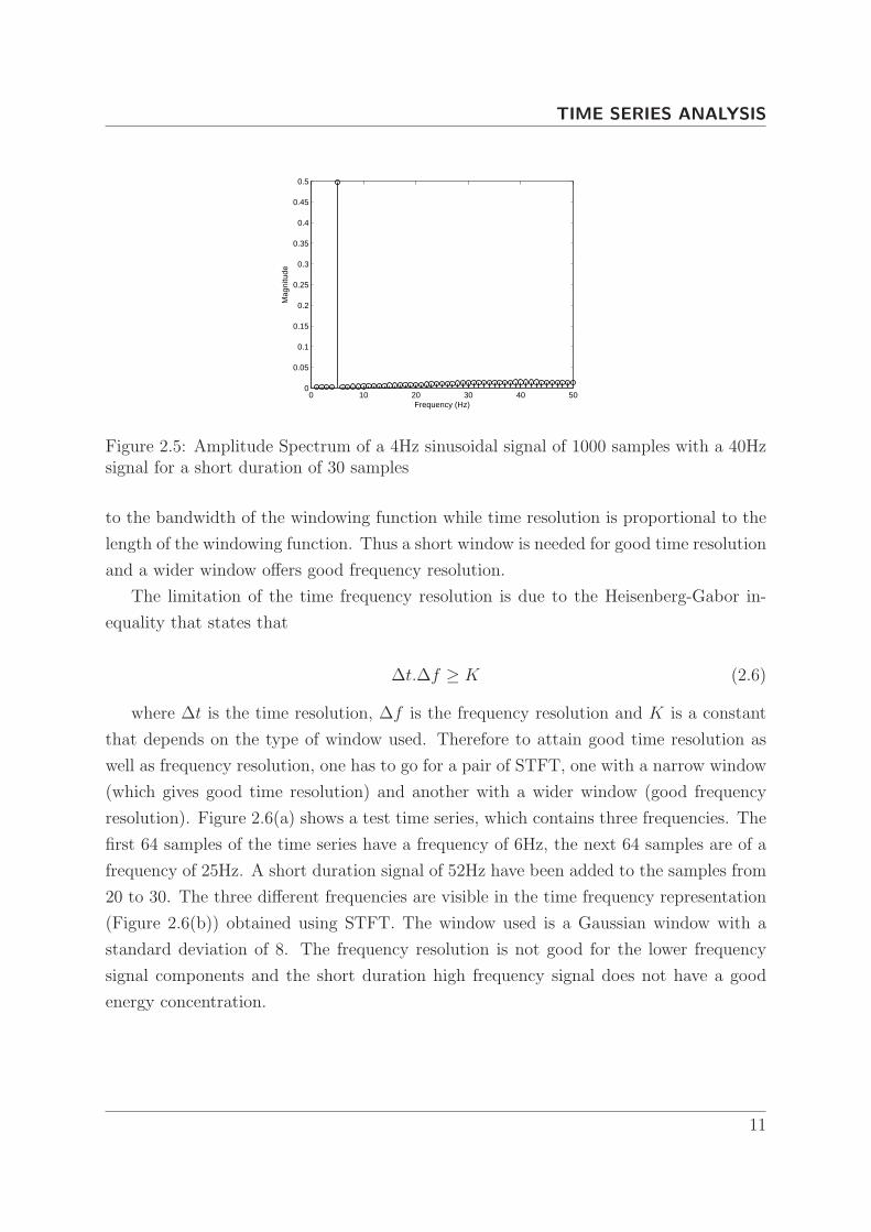
Figure 2.5: Amplitude Spectrum of a 4Hz sinusoidal signal of 1000 samples with a 40Hzsignal for a short duration of 30 samples
to the bandwidth of the windowing function while time resolution is proportional to the
length of the windowing function. Thus a short window is needed for good time resolution
and a wider window offers good frequency resolution.
The limitation of the time frequency resolution is due to the Heisenberg-Gabor in-
equality that states that
∆t.∆f ≥ K (2.6)
where ∆t is the time resolution, ∆f is the frequency resolution and K is a constant
that depends on the type of window used. Therefore to attain good time resolution as
well as frequency resolution, one has to go for a pair of STFT, one with a narrow window
(which gives good time resolution) and another with a wider window (good frequency
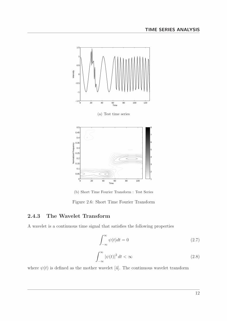
resolution). Figure 2.6(a) shows a test time series, which contains three frequencies. The
first 64 samples of the time series have a frequency of 6Hz, the next 64 samples are of a
frequency of 25Hz. A short duration signal of 52Hz have been added to the samples from
20 to 30. The three different frequencies are visible in the time frequency representation
(Figure 2.6(b)) obtained using STFT. The window used is a Gaussian window with a
standard deviation of 8. The frequency resolution is not good for the lower frequency
signal components and the short duration high frequency signal does not have a good
energy concentration.
11
Page 24
TIME SERIES ANALYSIS
0 20 40 60 80 100 120−1.5
−1
−0.5
0
0.5
1
1.5
Time
Inte
nsity
(a) Test time series
Time
Nor
mal
ized
Fre
quen
cy
0 20 40 60 80 1000
0.05
0.1
0.15
0.2
0.25
0.3
0.35
0.4
0.45
0.5
1
2
3
4
5
6
7
8
(b) Short Time Fourier Transform : Test Series
Figure 2.6: Short Time Fourier Transform
2.4.3 The Wavelet Transform
A wavelet is a continuous time signal that satisfies the following properties
∫∞
−∞
ψ(t)dt = 0 (2.7)
∫∞
−∞
|ψ(t)|2 dt <∞ (2.8)
where ψ(t) is defined as the mother wavelet [4]. The continuous wavelet transform
12
Page 25
TIME SERIES ANALYSIS
W (a, b) =
∫∞
−∞
y(t)ψ∗
a,b(t)dt (2.9)
where y(t) is any square integrable function,a is the dilation parameter, b is the trans-
lation parameter and ψ∗
a,b(t) is the dilation and translation(asterik denotes the complex
conjugate) of the mother wavelet defined as
ψ∗
a,b(t) =1√|a|ψ
(t− b
a
)(2.10)
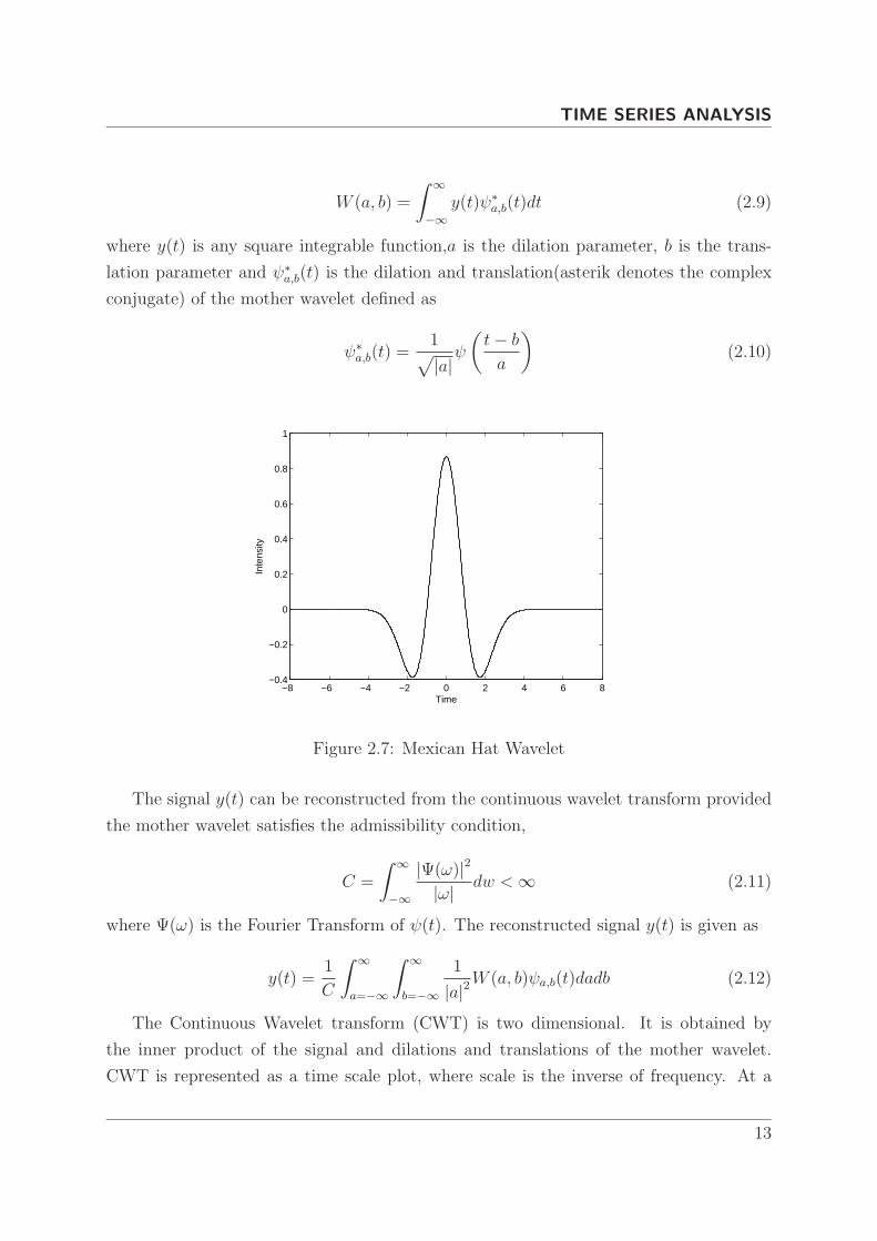
−8 −6 −4 −2 0 2 4 6 8−0.4
−0.2
0
0.2
0.4
0.6
0.8
1
Time
Inte
nsity
Figure 2.7: Mexican Hat Wavelet
The signal y(t) can be reconstructed from the continuous wavelet transform provided
the mother wavelet satisfies the admissibility condition,
C =
∫∞
−∞
|Ψ(ω)|2|ω| dw <∞ (2.11)
where Ψ(ω) is the Fourier Transform of ψ(t). The reconstructed signal y(t) is given as
y(t) =1
C
∫∞
a=−∞
∫∞
b=−∞
1
|a|2W (a, b)ψa,b(t)dadb (2.12)
The Continuous Wavelet transform (CWT) is two dimensional. It is obtained by
the inner product of the signal and dilations and translations of the mother wavelet.
CWT is represented as a time scale plot, where scale is the inverse of frequency. At a
13
Page 26
TIME SERIES ANALYSIS
low scale (high frequency), CWT offers high time resolution and at higher scales (lower
frequencies) CWT gives high frequency resolution. The interpretation of the time scale
representations produced by the wavelet transform require the knowledge of the type of
the mother wavelet (e.g. Mexican Hat (Figure 2.7),Gaussian etc.) used for the analysis.
Thus the visual analysis of the wavelet transform is intricate.
Time
Sca
le
20 40 60 80 100 120
1
2
3
4
5
6
7
8
9
10
50
100
150
200
Figure 2.8: The Wavelet Transform
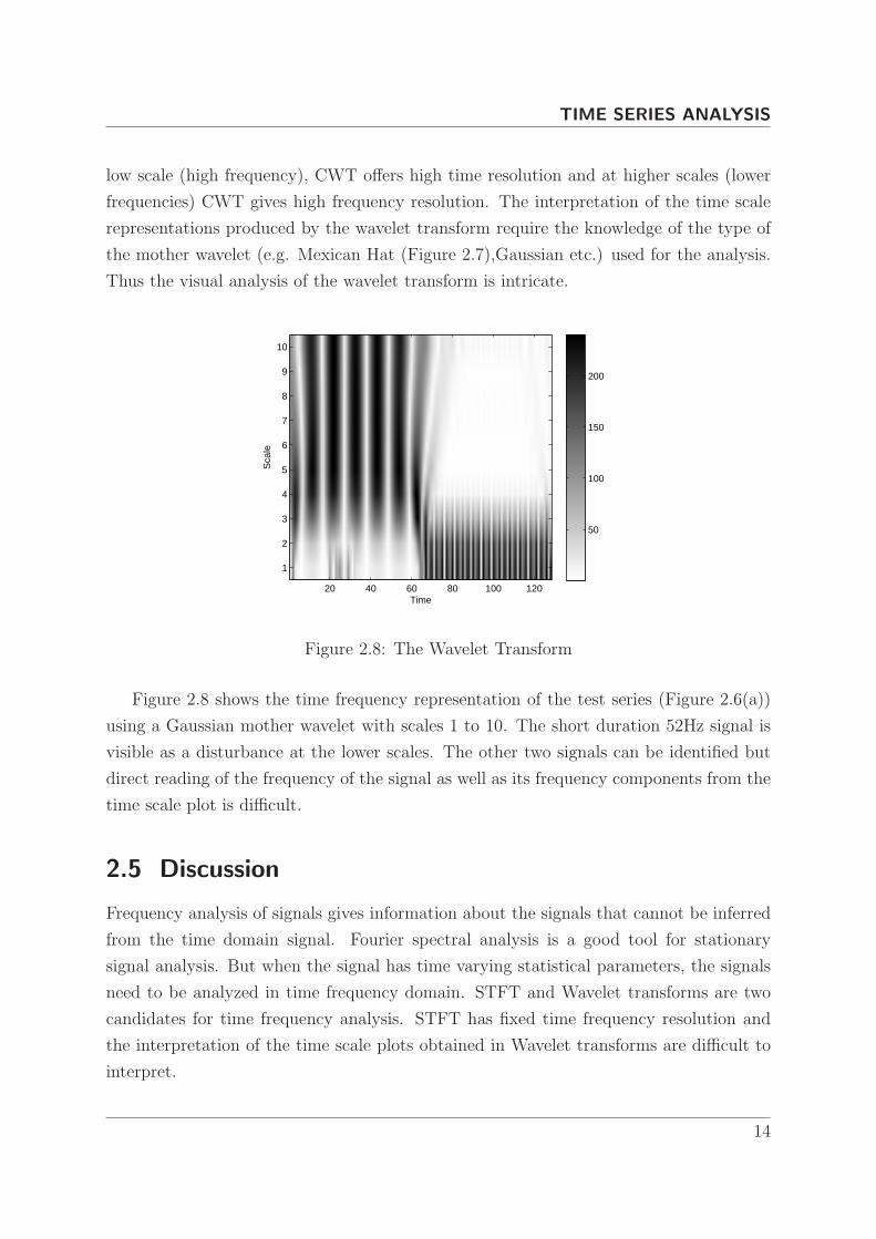
Figure 2.8 shows the time frequency representation of the test series (Figure 2.6(a))
using a Gaussian mother wavelet with scales 1 to 10. The short duration 52Hz signal is
visible as a disturbance at the lower scales. The other two signals can be identified but
direct reading of the frequency of the signal as well as its frequency components from the
time scale plot is difficult.
2.5 Discussion
Frequency analysis of signals gives information about the signals that cannot be inferred
from the time domain signal. Fourier spectral analysis is a good tool for stationary
signal analysis. But when the signal has time varying statistical parameters, the signals
need to be analyzed in time frequency domain. STFT and Wavelet transforms are two
candidates for time frequency analysis. STFT has fixed time frequency resolution and
the interpretation of the time scale plots obtained in Wavelet transforms are difficult to
interpret.
14
Page 27
3Modified S Transform
Page 28
MODIFIED S TRANSFORM
3.1 Introduction
The field of time frequency analysis got an impetus with the development of the Short
Time Fourier Transform (STFT). The STFT is a localized time frequency representation
of a time series. It uses a windowing function to localize the time and the Fourier
transform to localize the frequency. On account of the fixed width of the window function
used, STFT has poor time frequency resolution. The Wavelet Transform (WT) on the
other hand uses a basis function which dilates and contracts with frequency. The WT does
not retain the absolute phase information and the visual analysis of the time scale plots
that are produced by the WT is intricate. A time frequency representation developed
by Stockwell [5], which combines the good features of STFT and WT is called the S
transform. It can be viewed as a frequency dependent STFT or a phase corrected Wavelet
transform.
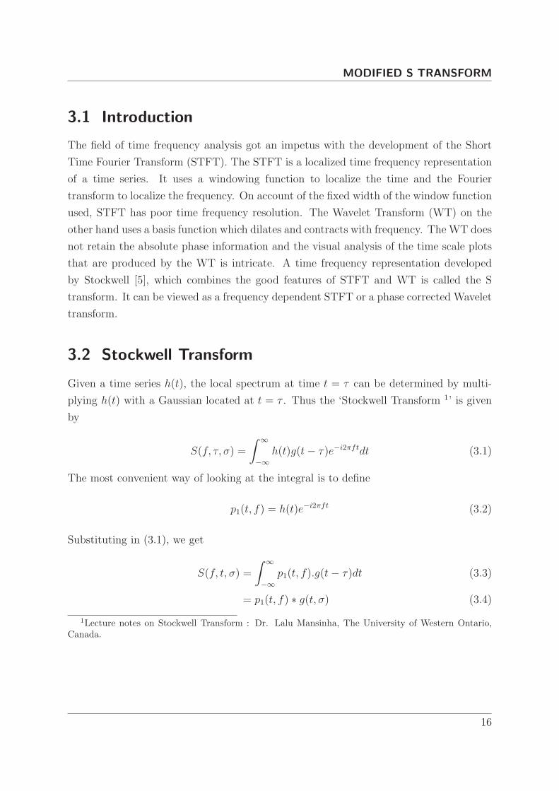
3.2 Stockwell Transform
Given a time series h(t), the local spectrum at time t = τ can be determined by multi-
plying h(t) with a Gaussian located at t = τ . Thus the ‘Stockwell Transform 1’ is given
by
S(f, τ, σ) =
∫∞
−∞
h(t)g(t− τ)e−i2πftdt (3.1)
The most convenient way of looking at the integral is to define
p1(t, f) = h(t)e−i2πft (3.2)
Substituting in (3.1), we get
S(f, t, σ) =
∫∞
−∞
p1(t, f).g(t− τ)dt (3.3)
= p1(t, f) ∗ g(t, σ) (3.4)
1Lecture notes on Stockwell Transform : Dr. Lalu Mansinha, The University of Western Ontario,Canada.
16
Page 29
MODIFIED S TRANSFORM
where ∗ denote the convolution operation. Let S(f, τ, σ) ↔ B(f, α, σ), where B(f, α, σ)
is the Fourier transform of S(f, τ, σ). Thus
S(f, τ, σ) =
∫∞
−∞
B(f, α, σ)e−i2πατdα (3.5)
From convolution theorem, we know that
{p1(t, f) ∗ g(t, σ)} ↔∫
∞
−∞
P1(f, α)e−2παtdα (3.6)
Since p1(f, t) = h(t).ei2πft,
P1(f, α) = H(α) ∗ δ(α− f) (3.7)
B(f, α, σ) = [H(α) ∗ δ(α− f)] .G(α, σ) (3.8)
S(f, τ, σ) =
∫∞
−∞
{[H(α) ∗ δ(α− f)] .G(α, σ)} e−i2πατdα (3.9)
B(f, α, σ) =
∫∞
−∞
S(f, τ, σ)ei2πατdτ (3.10)
B(f, α, σ) = [H(α) ∗ δ(α− f)] .G(α, σ) (3.11)
[H(α) ∗ δ(α− f)] =B(f, α, σ)
G(α, σ)(3.12)
Since H(α) ∗ δ(α − f) is the forward translation of H(α), we can perform a backward
translation to recover H(α) from H(α) ∗ δ(α− f).
H(α) ∗ δ(α− f) = H(α− f) (3.13)
H(α− f) =B(f, α, σ)
G(α, σ)(3.14)
H(α− f) ∗ δ(α, f) =
[B(f, α, σ)
G(α, σ)
]∗ δ(α+ f) (3.15)
H(α) =B(f, α+ f, σ)
G(α+ f, σ)(3.16)
Therefore S(f, τ, σ) is the transform of h(t) at t = τ and σ represents the width of
the Gaussian g(t). The sequence of operations for the calculation of S transform is
17
Page 30
MODIFIED S TRANSFORM
1. Determine
H(α) ↔ h(t)
G(α, σ) ↔ g(t, σ)
2. Calculate H(α) ∗ δ(α− f), which is H(α) translated to f .
3. Multiply G(α, σ) and shifted H(α)
4. Take the inverse Fourier Transform
For the original S transform, Stockwell and Mansinha made σ, the dilation parameter
a function of frequency f .
σ =1
f(3.17)
Thus the Gaussian window
g(t, σ) =1√2πσ
e−t2
2σ2 (3.18)
with σ = 1
fbecomes
g(t, σ) =f√2πσ
e−t2f2
2 (3.19)
and
G(α, f) = e−
2π2α2
f2 (3.20)
Equation 3.20 is derived from the Fourier Transform pair,
e−at2 ↔√π
ae−
ω2
4a (3.21)
which for a Gaussian function
g(t, σ) =1√2πσ
e−t2
2σ2 (3.22)
becomes
1√2πσ
e−t2
2σ2 ↔ 1√2πσ
√π2σ2e−
ω2
42σ2
(3.23)
↔ e−ω2σ2
2 (3.24)
18
Page 31
MODIFIED S TRANSFORM
The S-Transform can be defined as a CWT with a specific mother wavelet multiplied
by a phase factor.
S(τ, f) = ei2πftW (τ, d) (3.25)
where
W (τ, d) =
∫∞
−∞
h(t)w(t− τ)dt (3.26)
is the Wavelet Transform of a function h(t) with a mother wavelet w(t, f), defined as
w(t, f) =|f |√2πe−
t2f2
2 e−i2πft (3.27)
The S transform separates the mother wavelet into two parts,the slowly varying en-
velope (the Gaussian function) which localizes in time,and the oscillatory exponential
kernel e−2πft which selects the frequency being localized. It is the time localizing Gaus-
sian that is translated while the oscillatory exponential kernel remains stationary. By
not translating the oscillatory exponential kernel, the S-Transform localizes the real and
the imaginary components of the spectrum independently, localizing the phase spectrum
as well as the amplitude spectrum. This is referred to as absolutely referenced phase
information. The ST produces a time frequency representation instead of the time scale
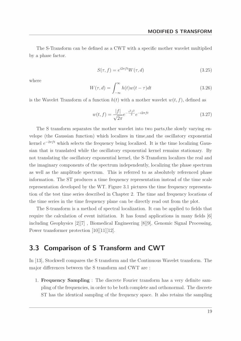
representation developed by the WT. Figure 3.1 pictures the time frequency representa-
tion of the test time series described in Chapter 2. The time and frequency locations of
the time series in the time frequency plane can be directly read out from the plot.
The S-transform is a method of spectral localization. It can be applied to fields that
require the calculation of event initiation. It has found applications in many fields [6]
including Geophysics [2][7] , Biomedical Engineering [8][9], Genomic Signal Processing,
Power transformer protection [10][11][12].
3.3 Comparison of S Transform and CWT
In [13], Stockwell compares the S transform and the Continuous Wavelet transform. The
major differences between the S transform and CWT are :
1. Frequency Sampling : The discrete Fourier transform has a very definite sam-
pling of the frequencies, in order to be both complete and orthonormal. The discrete
ST has the identical sampling of the frequency space. It also retains the sampling
19
Page 32
MODIFIED S TRANSFORM
Time
Nor
mal
ized
Fre
quen
cy
20 40 60 80 100 120
0.1
0.2
0.3
0.4
0.5
0.05
0.1
0.15
0.2
0.25
0.3
0.35
0.4
0.45
Figure 3.1: S Transform TFR of test time series
of the time series. On the other hand WT has a loosely defined scaling. It normally
employs an octave scaling for frequencies,which results in an oversampled represen-
tation at the low frequencies and an under sampled representation at the higher
frequencies.
2. Direct Signal Extraction : The amplitude, frequency and phase at any time
instant can be directly measured from the S transform. A time domain signal can
be extracted form the above measurements.
Signal(t) = A(t)cos(2 ∗ pi ∗ f(t) ∗ t+ φ(t)) (3.28)
where A(t),f(t) and φ(t) are the amplitude, frequency and phase at any time instant
t.This direct extraction of a signal is due to the combination of absolutely referenced
phase information and frequency invariant amplitude of the S-transform, and such
direct extraction cannot be done with Wavelet methods.
3. ST Phase : The ST retains the absolute phase information, where as the phase
information is lost in the WT. The absolutely referenced phase of the S-transform
is in contrast to a wavelet approach, where the phase of the wavelet transform is
relative to the center (in time) of the analyzing wavelet. Thus as the wavelet trans-
lates, the reference point of the phase translates. In ST, the sinusoidal component
20
Page 33
MODIFIED S TRANSFORM
of the basis function remains stationary, while the Gaussian envelope translates in
time. Thus the reference point for the phase remains stationary.
4. ST Amplitude : The unit area localizing function (the Gaussian) preserves the
amplitude response of the S-transform and ensures that the amplitude response of
the ST is invariant to the frequency. In much the same way that the phase of the
ST means the same as the phase of the Fourier transform, the amplitude of the ST
means the same as the amplitude of the Fourier transform. On the other hand, WT
diminishes the higher frequency components.
3.4 Generalized S Transform
McFadden et al. [14] and later Pinnegar and Mansinha [15] introduced a generalized
S-transform which has a greater control over the window function. The generalized S
transform is given by
S(τ, f, β) =
∫∞
−∞
h(t)w(τ − t, f, β)e−j2πftdt (3.29)
where w is the window function of the S transform and β denotes the set of parameters
that determine the shape and property of the window function. τ is a parameter that
controls the position of the Generalized window w on the time axis. For the Gaussian
window wGS [16], γ is the only parameter in β and it controls the width of the window
w(τ − t, f, γ) =|f |
γ√
2πexp
[−f
2(τ − t)2
2γ2
](3.30)
If the generalized window w satisfies the following normalization criteria,
∫∞
−∞
w(τ − t, f, β)dτ = 1 (3.31)
21
Page 34
MODIFIED S TRANSFORM
then
∫∞
−∞
S(τ − t, f, β)dτ =
∫∞
−∞
∫∞
−∞
h(t)e−i2πftw(τ − t, f, β)dtdτ (3.32)
=
∫∞
−∞
h(t)e−i2πft
∫∞
−∞
w(τ − t, f, β)dτdt (3.33)
=
∫∞
−∞
h(t)e−i2πftdt (3.34)
= H(f) (3.35)
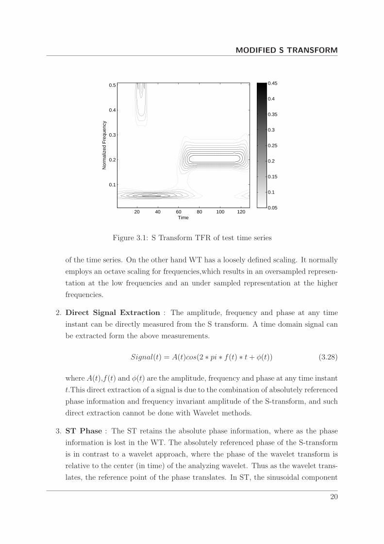
where H(f) is the Fourier transform of the signal h(t).
Frequency (f)
γ
b
Slope= η
Figure 3.2: Scaling function γ
3.5 Modified S Transform
In the modified S transform, we are using a different scaling rule for the Gaussian window.
The scaling function γ is made a linear function of frequency.
γ(f) = ηf + b (3.36)
where η is the slope and b is the intercept. The resolution in time and in frequency
depends on both η and b. We have determined usable values of η and b by trial and error.
22
Page 35
MODIFIED S TRANSFORM
The modified S transform becomes
S(τ, f, η, b) =
∫∞
−∞
h(t)w(τ − t, f, η, b)e−j2πftdt (3.37)
where w denotes the window function of the modified S transform, denoted by
w(τ − t, f, η, b) =|f |√
2π(ηf + b)e−
(τ−t)2f2
2(ηf+b)2 (3.38)
Using (3.37) and (3.38),
S(τ, f, η, b) =
∫∞
−∞
h(t)|f |√
2π(ηf + b)e−
(τ−t)2f2
2(ηf+b)2 e−j2πftdt (3.39)
The modified S transform also satisfies the normalization condition for S transform
windows and hence is invertible.
∫∞
−∞
|f |√2π(ηf + b)
e−
(τ−t)2f2
2(ηf+b)2 dτ = 1 (3.40)
0 20 40 60 80 100 1200
0.1
0.2
0.3
0.4
0.5
0.6
0.7
0.8
0.9
1
Time
Nor
mal
ised
Am
plitu
de
γ =0.5
γ =1
γ =2
Figure 3.3: Variation of window width with γ for a particular frequency(25Hz)
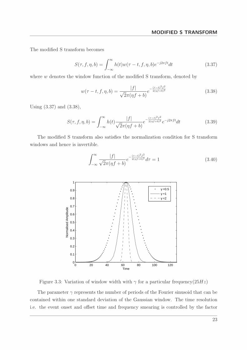
The parameter γ represents the number of periods of the Fourier sinusoid that can be
contained within one standard deviation of the Gaussian window. The time resolution
i.e. the event onset and offset time and frequency smearing is controlled by the factor
23
Page 36
MODIFIED S TRANSFORM
γ. If γ is too small the Gaussian window retains very few cycles of the sinusoid. Hence
the frequency resolution degrades at low frequencies. If γ is too high the window retains
more sinusoids within it and as a result the time resolution degrades at high frequencies.
It indicates that the γ value should be varied with care for better energy distribution in
the time-frequency plane.
Typical range of η is 0.25 − 0.5 and b is 0.5 − 3. The variation of width of window
with γ for a particular frequency component (25 Hz) is illustrated in Fig. 3.3. The value
of η and b need to be selected depending on the type and nature of the signal under
consideration.
Time
Nor
mal
ized
Fre
quen
cy
50 100 150 200 250 300
0.1
0.2
0.3
0.4
0.5
0.05
0.1
0.15
0.2
0.25
0.3
0.35
0.4
0.45
(a) Example 1 - TFR Using S Transform
Time
Nor
mal
ized
Fre
quen
cy
50 100 150 200 250 300
0.1
0.2
0.3
0.4
0.5
0.05
0.1
0.15
0.2
0.25
0.3
0.35
0.4
0.45
(b) Example 1 - TFR Using Modified S Transform
Figure 3.4: Example 1 - TFR Using S Transform and Modified S Transform
24
Page 37
MODIFIED S TRANSFORM
3.6 Simulation and Discussion
The time frequency resolution characteristics of the modified S transform is tested using
a set of test signals.
3.6.1 Example 1
The first test signal is a linear chirp signal. The instantaneous frequency of a linear chirp
signal varies linearly with time. The instantaneous frequency is given by
fi(t) = f0 + κt (3.41)
where
κ = (f1 − f0)/t1 (3.42)
κ ensures that the desired frequency breakpoint f1 at time t1 is maintained. f1 and f0
are two frequency points through which the signal traverses. For this example, the time
t is made to vary from -1 to 1.99 with a sampling period of 0.01 . The test signal can be
generated in MATLAB using the following commands.
t = −1 : 0.01 : 1.99;
h = chirp(t, 10, 1, 20);
Figure 3.4 shows the difference in time frequency resolution using S transform and
modified S transform with η = 0.25 and b = 1.9.
3.6.2 Example 2
The second test signal that is a combination of a linear and a quadratic chirp signal.
The frequency of the quadratic chirp increases quadratically. The linear chirp has a
frequency characteristics, that decreases linearly with time. The instantaneous frequency
of a quadratic chirp signal is given by
fi(t) = f0 + κt2 (3.43)
where
κ = (f1 − f0)/t2
1(3.44)
25
Page 38
MODIFIED S TRANSFORM
Time
Nor
mal
ized
Fre
quen
cy
50 100 150 200 250 300
0.1
0.2
0.3
0.4
0.5
0.1
0.2
0.3
0.4
0.5
0.6
0.7
0.8
(a) Example 2 - TFR Using S Transform
Time
Nor
mal
ized
Fre
quen
cy
50 100 150 200 250 300
0.1
0.2
0.3
0.4
0.5
0.1
0.15
0.2
0.25
0.3
0.35
0.4
0.45
0.5
0.55
0.6
(b) Example 2 - TFR Using Modified S Transform
Figure 3.5: Example 2 - TFR Using S Transform and Modified S Transform
κ ensures that the desired frequency breakpoint f1 at time t1 is maintained. f1 and
f0 are two frequency points through which the signal traverses. If f0 > f1, the chirp
signal will have a convex frequency behavior and if f1 > f0, the signal will have a concave
frequency pattern. The test signal can be generated in MATLAB using the following
commands
t = −1 : 0.01 : 1.99;
h = chirp(t, 10, 1, 15, ‘quadratic′) + chirp(t, 25, 1, 15);
Figure 3.5 depicts the TFR using original S transform and Modified S transform (η = 0.25
and b = 1.9). We can clearly see that the TFR using modified S transform has better
26
Page 39
MODIFIED S TRANSFORM
time frequency resolution compared to the original S transform.
3.7 Conclusion
The effective variation of the width of the Gaussian window can give better control
over the energy concentration for the S-transform. This is achieved by introducing an
additional parameter in the window which varies with frequency and thereby modulates
the S-transform kernel efficiently with the progress of frequency. The proposed scheme is
evaluated and compared with the standard S-transform by using a set of synthetic test
signals. The comparison shows that the proposed method is superior to the standard one,
providing a better time and frequency resolution. Hence the proposed S-transform can
be widely used for analysis of all kinds of signal that need more time as well as frequency
resolution.
27
Page 40
4Analysis of Business Cycles
Page 41
ANALYSIS OF BUSINESS CYCLES
4.1 Introduction
According to Parkin and Bade’s text “Foundations of Economics” [17],a business cycle
is the periodic but irregular up-and-down movements in economic activity, measured by
fluctuations in real GDP and other macroeconomic variables. A business cycle is not a
regular, predictable, or repeating phenomenon like the swing of the pendulum of a clock.
Its timing is random and, to a large degrees, unpredictable. A business cycle is identified
as a sequence of four phases:
• Contraction - A slowdown in the pace of economic activity
• Trough - The lower turning point of a business cycle, where a contraction turns into
an expansion
• Expansion - A speedup in the pace of economic activity
• Peak - The upper turning of a business cycle
A severe contraction is called a recession. A particularly long-lasting and painful
recession is known as a depression.
4.2 Causes of Business cycles
Just as there is no regularity in the timing of business cycles, there is no reason why cycles
have to occur at all[18]. The prevailing view among economists is that there is a level of
economic activity, often referred to as full employment, at which the economy could stay
forever. Full employment refers to a level of production in which all the inputs to the
production process are being used, but not so intensively that they wear out, break down,
or insist on higher wages and more vacations. When the economy is at full employment,
inflation tends to remain constant; only if output moves above or below normal does
the rate of inflation systematically tend to rise or fall. If nothing disturbs the economy,
the full-employment level of output, which naturally tends to grow as the population
increases and new technologies are discovered, can be maintained forever. There is no
reason why a time of full employment has to give way to either an inflationary boom or
a recession.
Business cycles do occur, however, because disturbances to the economy of one sort
or another push the economy above or below full employment. Inflationary booms can
29
Page 42
ANALYSIS OF BUSINESS CYCLES
be generated by surges in private or public spending. For example, if the government
spends a lot to fight a war but does not raise taxes, the increased demand will cause
not only an increase in the output of war matriel, but also an increase in the take-home
pay of defense workers. The output of all the goods and services that these workers
want to buy with their wages will also increase, and total production may surge above
its normal, comfortable level. Similarly, a wave of optimism that causes consumers to
spend more than usual and firms to build new factories may cause the economy to expand
more rapidly than normal. Recessions or depressions can be caused by these same forces
working in reverse. A substantial cut in government spending or a wave of pessimism
among consumers and firms may cause the output of all types of goods to fall.
Another possible cause of recessions and booms is monetary policy. The Federal
Reserve System strongly influences the size and growth rate of the money stock, and thus
the level of interest rates in the economy. Interest rates, in turn, are a crucial determinant
of how much firms and consumers want to spend. A firm faced with high interest rates
may decide to postpone building a new factory because the cost of borrowing is so high.
Conversely, a consumer may be lured into buying a new home if interest rates are low and
mortgage payments are therefore more affordable. Thus, by raising or lowering interest
rates, the Federal Reserve is able to generate recessions or booms. The following section
discusses the Economic indicators [19], which are parameters that are directly or indirectly
related to the economy and could possibly help in the analysis of business cycles.
4.3 Economic Indicators
An economic indicator is any economic statistic, such as the unemployment rate, GDP,
or the inflation rate, which indicate how well the economy is doing and how well the
economy is going to do in the future[18]. There are three major attributes each economic
indicator has:
1. Relation to business cycles
(a) Procyclic - A procyclic economic indicator is one that moves in the same
direction as the economy. So if the economy is doing well, this number is
usually increasing, whereas if we’re in a recession this indicator is decreasing.
The Gross Domestic Product (GDP) is an example of a procyclic economic
indicator.
30
Page 43
ANALYSIS OF BUSINESS CYCLES
(b) Countercyclic - A countercyclic economic indicator is one that moves in the
opposite direction as the economy. The unemployment rate gets larger as the
economy gets worse so it is a countercyclic economic indicator.
(c) Acyclic - An acyclic economic indicator is one that has no relation to the
health of the economy and is generally of little use.
2. Frequency of the Data
In most countries GDP figures are released quarterly (every three months) while
the unemployment rate is released monthly. Some economic indicators, such as the
Dow Jones Index, are available immediately and change every minute.
3. Timing
Economic Indicators can be leading, lagging, or coincident which indicates the
timing of their changes relative to how the economy as a whole changes.
(a) Leading - Leading economic indicators are indicators which change before
the economy changes. Stock market returns are a leading indicator, as the
stock market usually begins to decline before the economy declines and they
improve before the economy begins to pull out of a recession. Leading economic
indicators are the most important type for investors as they help predict what
the economy will be like in the future.
(b) Lagged - A lagged economic indicator is one that does not change direc-
tion until a few quarters after the economy does. The unemployment rate
is a lagged economic indicator as unemployment tends to increase for 2 or 3
quarters after the economy starts to improve.
(c) Coincident - A coincident economic indicator is one that simply moves at
the same time the economy does. The Gross Domestic Product is a coincident
indicator.
4.4 Types of business cycles
In [20], Schumpeter classifies business cycles based on their duration to five different
classes.
• Seasonal cycles - within a year
31
Page 44
ANALYSIS OF BUSINESS CYCLES
• Kitchin cycles - 3 years
• Juglar cycles - 9-10 years
• Kuznets cycles - 15-20 years
• Kondratiev cycles - 48-60 years
He also defines a ‘cycle’ as a loop of four stages : boom-recession-depression-recovery.
Starting from the mean, a boom is a rise which lasts until the peak is reached; a recession
is the drop from the peak back to the mean; a depression is the slide from the mean down
to the trough; a recovery is the rise from the trough back up to the mean. From the
mean, we then move up into another boom and thus the beginning of another four-phase
cycle. In a sense, any cycle of whatever duration can be described as going through these
four phases.
4.4.1 Kondratiev cycles
Kondratiev or K-waves are regular, sinusoidal cycles in the modern world economy. Av-
eraging fifty and ranging from approximately forty to sixty years in length, the cycles
consist of alternating periods between high sectoral growth and periods of slower growth.
Simon Kuznets,(1901-1985) classifies Kondratiev cycles or long waves into four major
classes.
• The Industrial Revolution (1787-1842)- The industrial revolution cycle is the
most famous Kondratiev wave. The boom began in about 1787 and turned into a
recession at the beginning of the Napoleonic age in 1801 and, in 1814, deepened
into a depression. The depression lasted until about 1827 after which there was
a recovery until 1842. As is obvious, this Kondratiev rode on the development of
textile, iron and other steam-powered industries.
• The Bourgeois Kondratiev (1843-1897): After 1842, the boom reemerged and
a new Kondratiev wave began, this one as a result of the development of road and
rail networks in Northern Europe and America and the accompanying expansion
in the coal and iron industries. The boom ended approximately in 1857 when it
turned into a recession. The recession turned into a depression into 1870, which
lasted until about 1885. The recovery began after that and lasted until 1897.
32
Page 45
ANALYSIS OF BUSINESS CYCLES
• The Neo-Mercantilist Kondratiev (1898-1950): The boom began about 1898
with the expansion of electric power and the automobile industry and lasted until
about 1911. The recession which followed turned into depression in about 1925
which lasted until around 1935.
• The Fourth Kondratiev (1950- 2000) : There has been much debate among
econometricians on the dating the Fourth Wave - largely because of the confusions
generated by the low fluctuation in price levels and the issue of Keynesian policies
and hence this debate is yet to be resolved. Perhaps the most acceptable set of
dates is that the boom began around 1950 and lasted until about 1974 wherein
recession set in. In and around 1981 there was a depression followed by a recovery
that lasted upto around 1992.
1950 1960 1970 1980 1990 20000
2000
4000
6000
8000
10000
12000
Year
Mon
thly
Ave
rage
Clo
sing
Pric
e (D
JIA
)
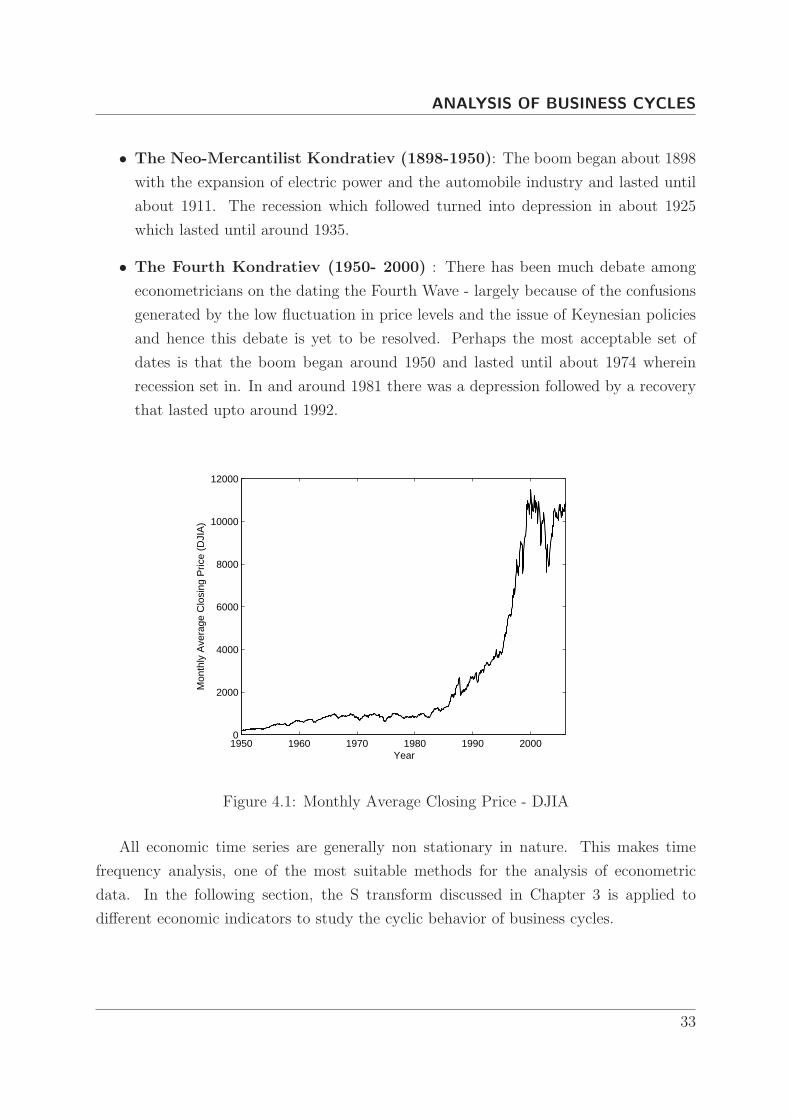
Figure 4.1: Monthly Average Closing Price - DJIA
All economic time series are generally non stationary in nature. This makes time
frequency analysis, one of the most suitable methods for the analysis of econometric
data. In the following section, the S transform discussed in Chapter 3 is applied to
different economic indicators to study the cyclic behavior of business cycles.
33
Page 46
ANALYSIS OF BUSINESS CYCLES
4.5 Analysis and Discussion
1950 1960 1970 1980 1990 20000
200
400
600
800
1000
1200
1400
1600
Year
Mon
thly
Ave
rage
Clo
sing
Pric
e (S
& P
500
)
Figure 4.2: Monthly Average Closing Price - S&P 500
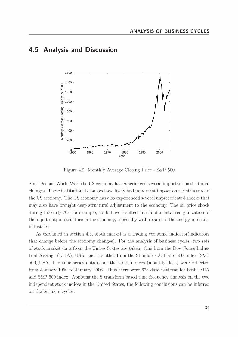
Since Second World War, the US economy has experienced several important institutional
changes. These institutional changes have likely had important impact on the structure of
the US economy. The US economy has also experienced several unprecedented shocks that
may also have brought deep structural adjustment to the economy. The oil price shock
during the early 70s, for example, could have resulted in a fundamental reorganization of
the input-output structure in the economy, especially with regard to the energy-intensive
industries.
As explained in section 4.3, stock market is a leading economic indicator(indicators
that change before the economy changes). For the analysis of business cycles, two sets
of stock market data from the Unites States are taken. One from the Dow Jones Indus-
trial Average (DJIA), USA, and the other from the Standards & Poors 500 Index (S&P
500),USA. The time series data of all the stock indices (monthly data) were collected
from January 1950 to January 2006. Thus there were 673 data patterns for both DJIA
and S&P 500 index. Applying the S transform based time frequency analysis on the two
independent stock indices in the United States, the following conclusions can be inferred
on the business cycles.
34
Page 47
ANALYSIS OF BUSINESS CYCLES
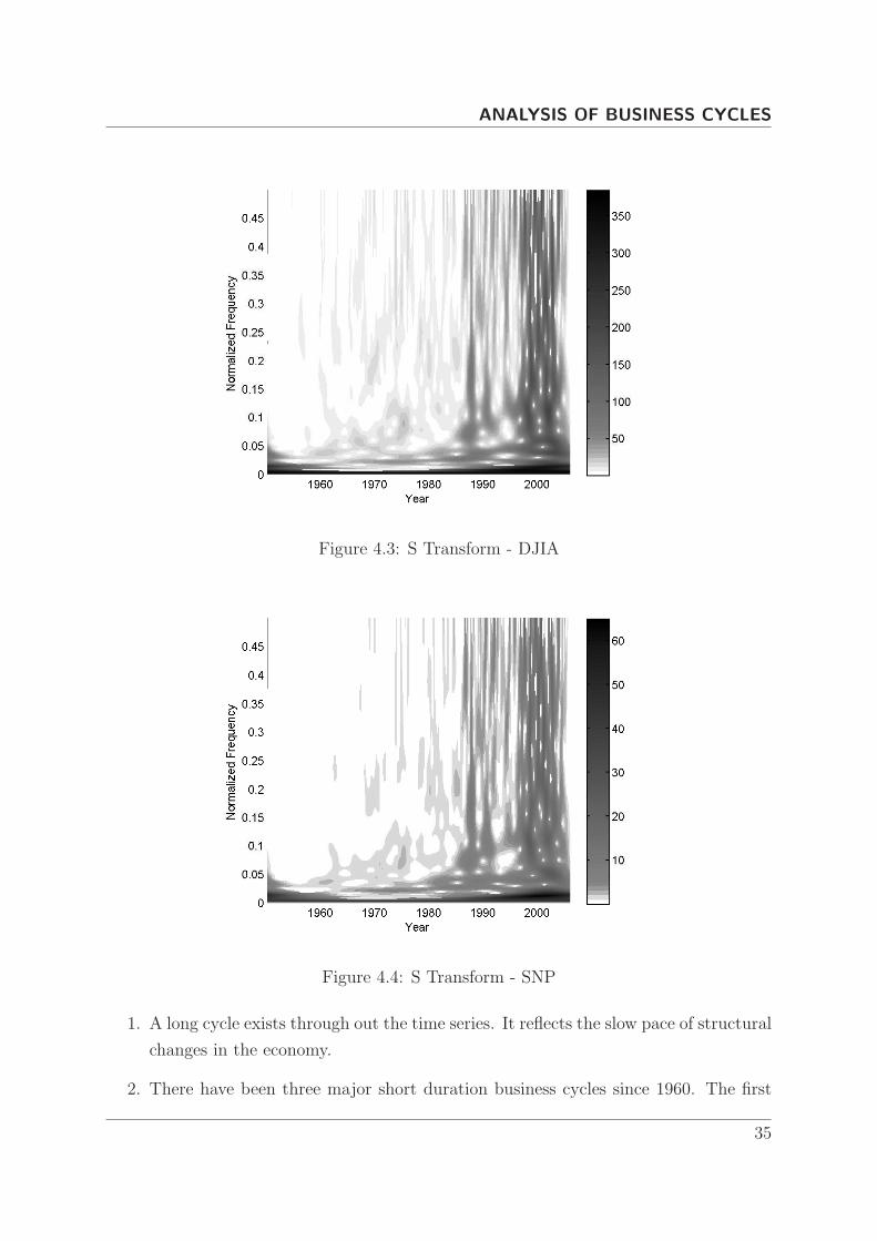
Figure 4.3: S Transform - DJIA
Figure 4.4: S Transform - SNP
1. A long cycle exists through out the time series. It reflects the slow pace of structural
changes in the economy.
2. There have been three major short duration business cycles since 1960. The first
35
Page 48
ANALYSIS OF BUSINESS CYCLES
1950 1960 1970 1980 1990 20002
3
4
5
6
7
8
9
10
11
Year
Per
cent
age
Une
mpl
oyed
(U
.S)
Figure 4.5: Percentage Unemployed (U.S)
occurred in 1961, triggered by a sharp external impulse during that year. The 1961
cycle has a frequency of 30 months per cycle and is short lived.
3. The second major cycle took place in 1973, apparently triggered by two impulses
during 1972 and 1973, and was greatly intensified by another impulse near 1975
[21]. This business cycle lasted about 3-4 years and peaked at the frequency of
about 70 months per cycle).
4. The third major cycle occurred during 1982-1984, apparently triggered by a shock
in 1982. This cycle lasted about 3 years and peaked also at a frequency similar to
the 1973 cycle.
5. There exists a short-lived business cycle in 1966 triggered by an external impulse.
According to International Monetary Fund (IMF) working paper on the evolution
of business cycles [22] , the nature of world business cycles has changed over time due
to ‘globalization’, which is often associated with rising trade and financial linkages. It
is indeed the case that globalization has picked up momentum in recent decades. For
example, the cumulative increase in the volume of world trade is almost three times
larger than that of world output since 1960. More importantly, there has been a striking
increase in the volume of international financial flows during the past two decades as
36
Page 49
ANALYSIS OF BUSINESS CYCLES
Figure 4.6: S Transform TFR - Unemployment
these flows have jumped from less than 5 percent to approximately 20 percent of GDP of
industrialized countries. Recent empirical studies are also unable to provide a concrete
explanation for the impact of stronger trade and financial linkages on the nature of
business cycles.
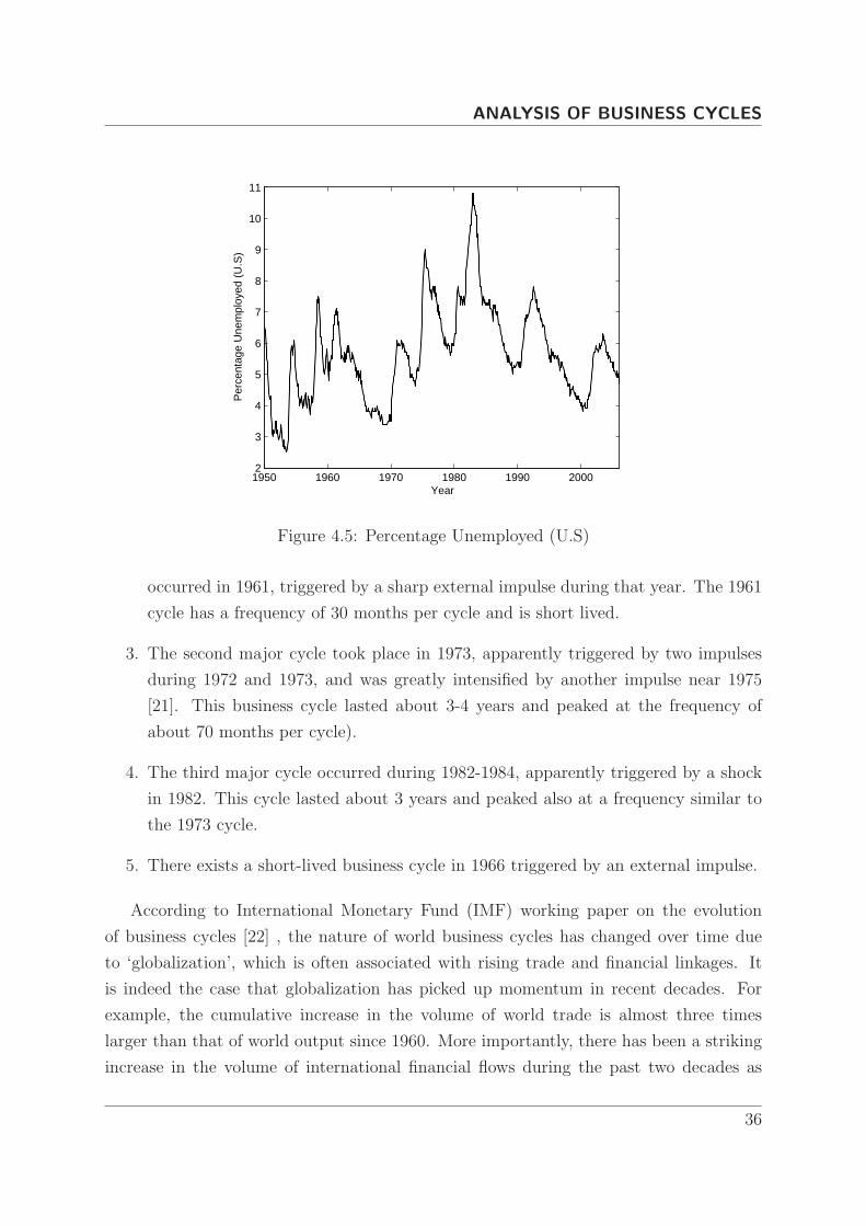
Similar to the stock prices, percentage unemployed in a country is a direct indicator
of the condition of an economy. In order to study the behavior of unemployment, a time
frequency analysis was done on the United States Percentage Unemployed data. The
data was collected from January 1950 to January 2006, the same period of study of the
stock market time series. The unemployment rate time series (Figure 4.5) show a cyclic
behavior, but the frequency of the cycle cannot be inferred directly from the time domain
signal. Figure 4.6 depicts the time frequency representation of the unemployment rate
time series using S transform. There exists a low frequency cycle at around 0.02 (nor-
malized frequency).Time period of the unemployment cycle = 1/0.02 = 50 months,which
turns out to be very close to the presidential tenure in the United States (4 years).
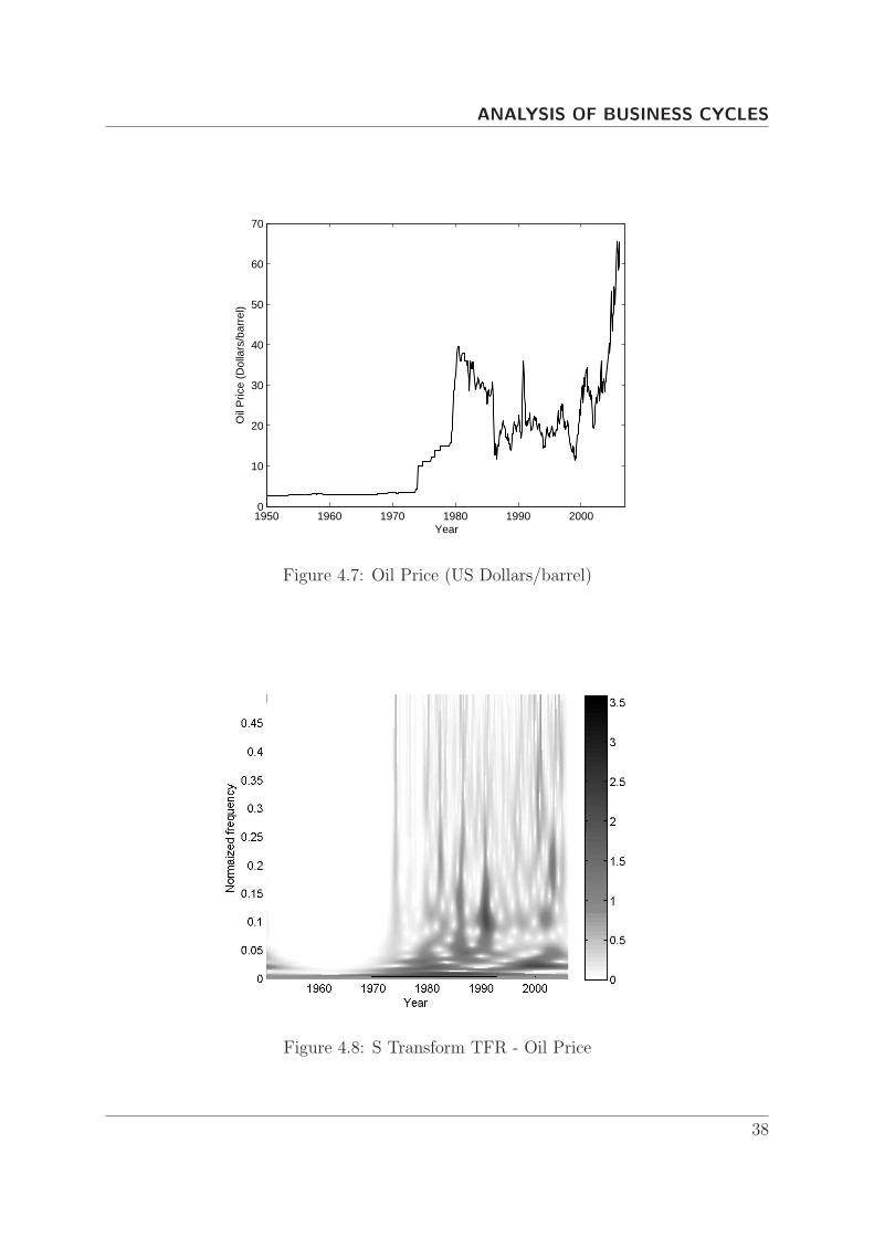
Oil price is an economic indicator which can directly affect the state of the world
economy. The rise in oil price can lead to economic crisis. Figure 4.7 shows the oil
price in US dollars/barrel from January 1950 to January 2006 (673 data samples). The
time frequency analysis of oil price (Figure 4.8) reveals that there is repetitive cycle of
around 0.1 (Normalized Frequency), which repeats itself in 1974,1981,1983,1986,1990-
37
Page 50
ANALYSIS OF BUSINESS CYCLES
1950 1960 1970 1980 1990 20000
10
20
30
40
50
60
70
Year
Oil
Pric
e (D
olla
rs/b
arre
l)
Figure 4.7: Oil Price (US Dollars/barrel)
Figure 4.8: S Transform TFR - Oil Price
38
Page 51
ANALYSIS OF BUSINESS CYCLES
91 and 2001. The possible reason(s) for the 0.1 frequency cycle is pictured in Table
4.1,where the cycles are in close match with the oil price peaks observed by Walter Labys
[23]. There also exists another low frequency component that exists almost through out
the duration of study. The low frequency is around 50 months which is coinciding with
both the unemployment cycle, which in turn almost matches with the US presidency
cycle.
Table 4.1: Oil Price Peaks
Year Possible Reason
1974 Arab oil production embargo
1979 Fall of the Shah of Iran
1981 Afghan War
1983 Afghan War
1986 Iran-Iraq War
1991 Gulf War
2001 Iraq-US War
4.6 Conclusion
The time frequency analysis of economic indicators have revealed the existence of business
cycles of different durations in an econometric time series. The relation between unem-
ployment, oil price and the economic situation of a country could be identified from the
study. The analysis results can be combined with other economic indicators to forecast
the behavior of global economy.
39
Page 52
5Time Frequency Filtering
- An Alternate Approach
Page 53
TIME FREQUENCY FILTERING
- AN ALTERNATE APPROACH
5.1 Introduction
Standard frequency domain filtering approaches have a fixed stop band and pass band
for the entire time duration.Since most of the natural time series are non-stationary,
there is a need for filters with variable pass bands and stop bands. Linear time-varying
(LTV) filter is such type of a filter which have a dynamic cutoff frequency. i.e. The
cutoff frequency varies with time. LTV filters have important applications including
non-stationary statistical signal processing (signal detection and estimation, spectrum
estimation, etc.) and communications over time-varying channels (interference excision,
channel modeling, estimation, equalization, etc.). LTV filters are particularly useful for
weighting, suppressing or separating non-stationary signal components[24].
The input output relation for a linear time varying filter, H, is given by
y(n) = H.x(n) (5.1)
where x(n) is the filter input and y(n) is the LTV filter output.
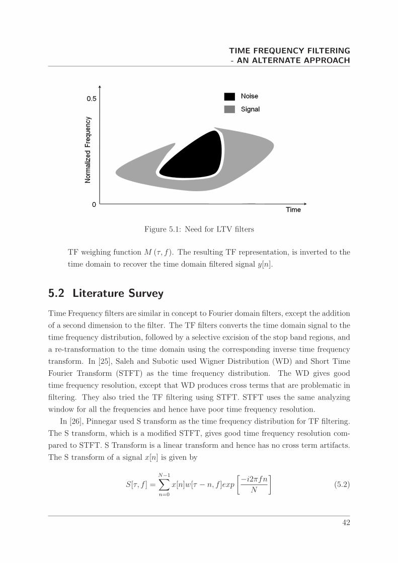
Time Frequency (TF) representations can be used to implement a LTV filter, when
either x(n), y(n) or H is non-stationary. The need for a time varying filter can be
explained using Figure 5.1. The figure represents the time frequency representation of
a synthetic signal. The synthetic signal is composed of two time series. One is a noise
component, which is represented by the black region of the TF representation. The
grey region shows the signal component of the composite signal. A filter need to be
designed to remove the noise component of the composite signal without affecting the
signal component. The filter H should pass the signal components and should block the
noise components. These type of signals cannot be filtered using a Fourier domain filter
as the cutoff frequency is different at different time locations (i.e. varying with time). A
possible solution is the time varying filter, whose cutoff frequency varies with time. The
specification of the filter H can be expressed as a TF weighting function, M (τ, f), which
is effectively ‘1’ over the signal regions and is ‘0’ for the noise regions.
The two different general approaches to designing a Linear Time Varying filters are -
1. Explicit Design - The LTV filter H is designed to closely match the weighing
function,M(τ, f). The filtering is performed in the time domain using (5.1).
2. Implicit Design - The LTV filter H is designed implicitly during the filtering,
which is an analysis-weighting-synthesis procedure. A linear TF representation of
the input signal x[n] is first calculated. The TF representation is multiplied by the
41
Page 54
TIME FREQUENCY FILTERING
- AN ALTERNATE APPROACH
Figure 5.1: Need for LTV filters
TF weighing function M (τ, f). The resulting TF representation, is inverted to the
time domain to recover the time domain filtered signal y[n].
5.2 Literature Survey
Time Frequency filters are similar in concept to Fourier domain filters, except the addition
of a second dimension to the filter. The TF filters converts the time domain signal to the
time frequency distribution, followed by a selective excision of the stop band regions, and
a re-transformation to the time domain using the corresponding inverse time frequency
transform. In [25], Saleh and Subotic used Wigner Distribution (WD) and Short Time
Fourier Transform (STFT) as the time frequency distribution. The WD gives good
time frequency resolution, except that WD produces cross terms that are problematic in
filtering. They also tried the TF filtering using STFT. STFT uses the same analyzing
window for all the frequencies and hence have poor time frequency resolution.
In [26], Pinnegar used S transform as the time frequency distribution for TF filtering.
The S transform, which is a modified STFT, gives good time frequency resolution com-
pared to STFT. S Transform is a linear transform and hence has no cross term artifacts.
The S transform of a signal x[n] is given by
S[τ, f ] =N−1∑
n=0
x[n]w[τ − n, f ]exp
[−i2πfnN
](5.2)
42
Page 55
TIME FREQUENCY FILTERING
- AN ALTERNATE APPROACH
where n and f are integer time and frequency indices. If T represents the sampling
interval, nT gives the time in seconds and f/NT gives the frequency in Hz. The position of
the S transform window w, is given by τ . The major difference between the STFT and the
S transform is in the window function used. In STFT, a sliding window is used, whereas
in S transform, a sliding window which scales in amplitude and width with frequency
is used. A Gaussian window with an inverse relation between standard deviation σ and
frequency f is normally used. The window function w[τ − n, f ] is presented in 5.3.
w[τ − n, f ] =|f |
N√
2πexp
[f 2(τ − n)2
2N2
](5.3)
The width of the Gaussian part of w, as measured between the peak and the point
having 1/√e the peak amplitude, is equal to N/ |f || , the wavelength of the fth Fourier
sinusoid. Thus, at any f , w always retains the same number of Fourier cycles[26]. The S
transform is an invertible time frequency transform. The invertibility of the S transform
depends on the window used in the analysis. For the S transform to be invertible, the
window w should satisfy the normalization condition given by
N−1∑
τ=0
w [τ − n, f ] = 1 (5.4)
When summed over all values of τ , the S transform (5.2) collapses to the Discrete
Fourier Transform(DFT), X(f).
X[f ] =N−1∑
τ=0
S[τ, f ] (5.5)
An inverse DFT recovers the original time domain signal from the time frequency
representation of S transform. The inverse S transform is given by
x[n] =1
N
N/2−1∑
f=−N/2
N−1∑
τ=0
S[τ, f ]exp
[i2πft
N
](5.6)
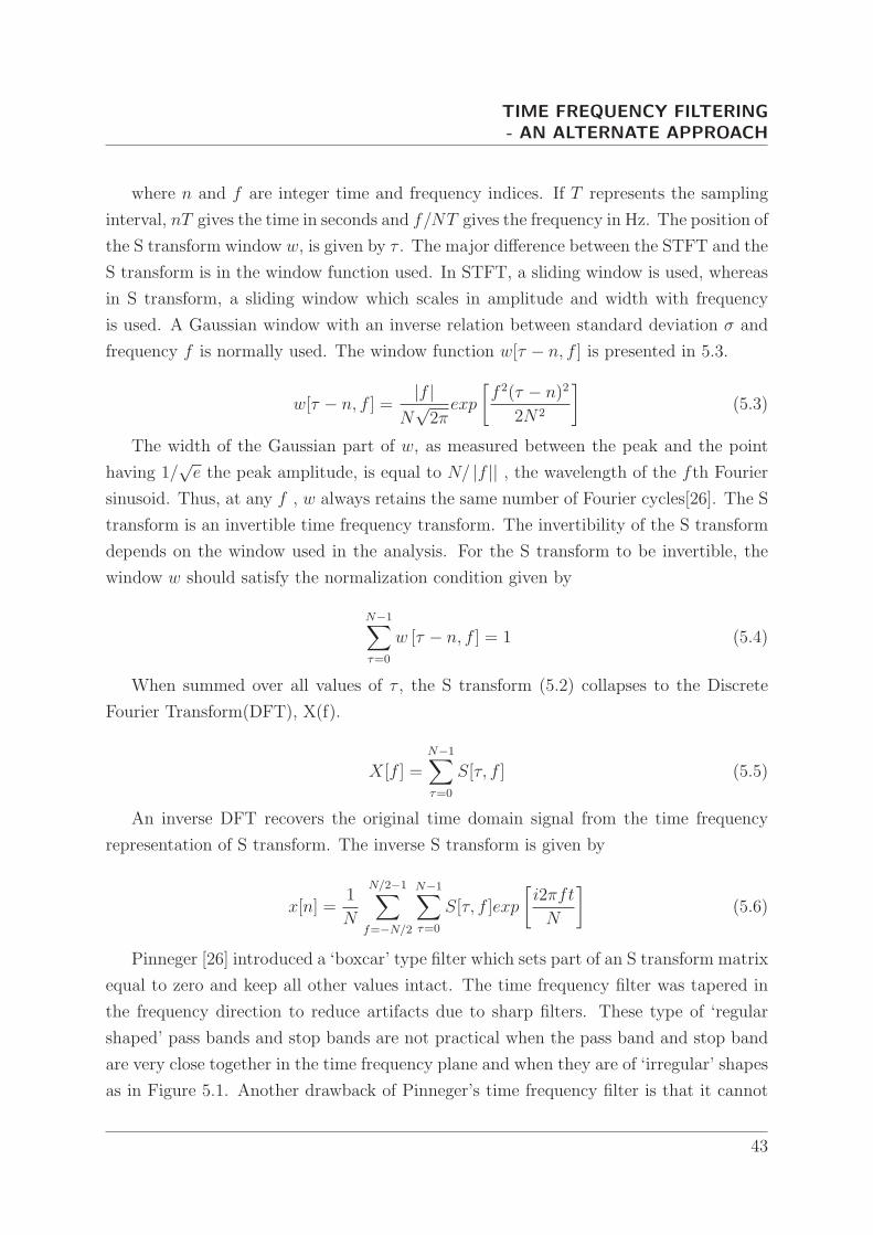
Pinneger [26] introduced a ‘boxcar’ type filter which sets part of an S transform matrix
equal to zero and keep all other values intact. The time frequency filter was tapered in
the frequency direction to reduce artifacts due to sharp filters. These type of ‘regular
shaped’ pass bands and stop bands are not practical when the pass band and stop band
are very close together in the time frequency plane and when they are of ‘irregular’ shapes
as in Figure 5.1. Another drawback of Pinneger’s time frequency filter is that it cannot
43
Page 56
TIME FREQUENCY FILTERING
- AN ALTERNATE APPROACH
remove background noise (Additive white Gaussian (AWG) Noise) , if any, present in the
signal. The AWG noise in the time domain is usually spread across the complete time
frequency plane, including the pass band. The filter in [26][27] can remove the AWG
noise in the stop band as the complete signal in the stop band is removed. But it is not
the case with the pass band. The AWG noise in the pass band of the filter remains in
the filtered signal and hence is difficult to remove. The above mentioned two problems
can be solved to a great extend using the following filtering approach.
5.3 The Proposed Filtering Approach
This novel filtering process is performed in two stages. In the first phase, the background
noise is removed and then in the second stage the time limited and band limited noise
components of the time series is removed. The filtering process kicks off with a time
frequency representation of a time series using the modified S transform developed in
Chapter 2. The modified S transform is used instead of the normal S transform as it
gives better energy concentration than the original S transform.
5.3.1 Background Noise Removal
A low order ‘best fit’ surface is first developed by least square fitting of the |S(τ, f)| . This
surface acts as a reference for removing background noise. The difference between the S
transform plane and the best fit quadratic surface is derived to form an intermediate sur-
face. All data on the intermediate surface, which are less than three standard deviations
of the Fourier transform are considered as part of the background noise spectrum and
are removed from the S transform plane. For time series with very high signal amplitude
compared to the background noise, a two stage fitting process is executed. An initial
surface fitting is used to remove the highly prominent signal components from the time
frequency plane. Another surface is fitted on the new time frequency plane obtained,
which represents the true nature of the background noise, and is used as the reference
surface for excision of background noise.
5.3.2 Localised Noise Filtering
The S transform plane obtained after background noise removal can be used as a foun-
dation for filtering out localized unwanted signal elements. The ST plane is converted
to a gray scale image, and the edges of the image are determined using a ‘Laplacian for
44
Page 57
TIME FREQUENCY FILTERING
- AN ALTERNATE APPROACH
Gaussian’ edge detection technique. The Laplacian is a 2-D isotropic measure of the 2nd
spatial derivative of an image. The Laplacian of an image highlights regions of rapid
intensity change. The Laplacian is applied to the image after smoothing the image with
a spatial Gaussian filter in order to reduce its sensitivity to noise. If I(x, y) denote the
pixel intensity values of an image, the Laplacian, L(x, y) can be calculated as:
L(x, y) =∂2I
∂x2+∂2I
∂y2(5.7)
This operation produces an image that shows the edges of the signal and noise area
as closed loops. The signal signatures which needed to be retained are ‘whiteouted’ using
image filling techniques. Morphological dilation [28] is applied on the image to slightly
‘grow’ the signal regions in all directions on the image. The growth is intentionally made
more prominent in the frequency direction of the S transform plane to reduce the artifacts
of boxcar type filtering. The image after dilation forms a filter mask which is essentially
the weighing function M (τ, f) described in Section 5.1. The product of the S transform
surface and the filter mask removes the noise signatures. An Inverse S transform of the
newly obtained S transform plane using (5.6) gives the filtered signal.
0 50 100 150 200 250−3
−2
−1
0
1
2
3
Time
Mag
nitu
de
Figure 5.2: Example 1 - Input Signal
45
Page 58
TIME FREQUENCY FILTERING
- AN ALTERNATE APPROACH
5.4 Simulation and Discussions
The performance of the filtering approach was tested using two different types of exam-
ples.
5.4.1 Example 1
Time
Nor
mai
zed
Fre
quen
cy
50 100 150 200 250
0.1
0.2
0.3
0.4
0.5
0.05
0.1
0.15
0.2
0.25
0.3
0.35
0.4
0.45
0.5
Figure 5.3: Example 1 - S Transform of the input signal
Figure 5.2 shows the first time series that was taken for the performance evaluation. The
time series consists of four sets of sinusoidals at three different frequencies. The first
sinusoidal is a 20Hz sinusoidal signal, which extends across the full length of the time
series. The second signal is a 35Hz signal, which extends from samples 50 to 125 and
from 150 to 225. The fourth set consists of a 50Hz sinusoidal signal which is time limited
from 100 to 200 samples.
Figure 5.3 depicts the S transform contour plot of the test signal using the modified
S transform with the parameters η = 0.25 and b = 1.9. The change in the S transform
contour with the addition of Additive White Gaussian Noise (AWGN)can be clearly seen
in Figure 5.4, which is the S transform contour of the test signal with a signal to noise
ratio (SNR) of 10dB. A single stage quadratic surface (Figure 5.6) fitting was used for
the first example to remove background noise. The 35Hz signal from samples 150 to
46
Page 59
TIME FREQUENCY FILTERING
- AN ALTERNATE APPROACH
Time
Nor
mal
ized
Fre
quen
cy
50 100 150 200 250
0.1
0.2
0.3
0.4
0.5
0.05
0.1
0.15
0.2
0.25
0.3
0.35
0.4
0.45
0.5
0.55
Figure 5.4: Example 1 - S transform of the input signal (SNR=10dB)
225 is considered here as an inband noise (i.e: 35Hz sinusoidal is part of the pass band
from samples 50 to 125 and is part of the stop band from samples 150 to 225. The same
frequency is present in the pass band and stop band).
Figure 5.5: Example 1 - Weighing Function
Using the image based techniques described in Section 5.3.2, a weighing function as
shown in Figure 5.5 is obtained and is multiplies with the S transform surface to remove
the inband noise. Figure 5.7 shows the desired filter output time series and the actual
filter output time series. The filtering efficiency was quantitatively measured using the
mean squared error (MSE).
47
Page 60
TIME FREQUENCY FILTERING
- AN ALTERNATE APPROACH
Figure 5.6: Example 1 - Noise Base
0 50 100 150 200 250−3
−2
−1
0
1
2
3
Time
Inte
nsity
Desired OutputActual Output
Figure 5.7: Example 1 - Filter Output
MSE =
∑N [x(n) − x̃(n)]2
N(5.8)
where x(n) is the original time series, x̃(n) is the filtered time series and N is the length
48
Page 61
TIME FREQUENCY FILTERING
- AN ALTERNATE APPROACH
of the time series. Table 5.1 shows the MSE for different values of SNR for the first
example.
Table 5.1: Error Analysis : Example 1
SNR (dB) MSE
10 0.0400
20 0.0293
30 0.0286
40 0.0277
5.4.2 Example 2
The second test series (Figure 5.8) contains two quadratic chirp signals: one is a time
localized chirp and the other one is present across the full length of the time series. The
time series is corrupted by AWGN.
0 50 100 150 200 250 300−2
−1.5
−1
−0.5
0
0.5
1
1.5
2
Time
Inte
nsity
Figure 5.8: Example 2 - Input Signal
Figure 5.9 shows the TFR of the original time series , using the modified S transform
49
Page 62
TIME FREQUENCY FILTERING
- AN ALTERNATE APPROACH
with the parameters η = 0.25 and b = 1.9. Figure 5.10 depicts the TFR of the test series
corrupted with AWGN at an SNR of 10dB. On the TFR there appears a low magnitude
background t-f spectrum (AWGN), with visible high magnitude spectral t-f components,
which are the two chirp waveforms.
Time
Nor
mai
zed
Fre
quen
cy
50 100 150 200 250 300
0.1
0.2
0.3
0.4
0.5
0.05
0.1
0.15
0.2
0.25
0.3
0.35
0.4
0.45
0.5
Figure 5.9: Example 2 - TFR using modified S transform
Time
Nor
mai
zed
Fre
quen
cy
50 100 150 200 250 300
0.1
0.2
0.3
0.4
0.5
0.05
0.1
0.15
0.2
0.25
0.3
0.35
0.4
0.45
0.5
0.55
Figure 5.10: Example 2 - TFR of noisy signal using modified S transform
50
Page 63
TIME FREQUENCY FILTERING
- AN ALTERNATE APPROACH
Figure 5.11: Example 2 - Reference surface for filtering out background noise
Since the test series has different amplitudes at different regions of time, a two stage
curve fitting technique is employed. In the first stage fitting a quadratic ‘best fit’ surface
is fitted to |S(τ, f)|, the absolute value of the S transform matrix. This surface is used
as a reference surface to remove the high amplitude signal components.
Time
Nor
mal
ized
Fre
quen
cy
50 100 150 200 250 300
0.1
0.2
0.3
0.4
0.5
0.05
0.1
0.15
0.2
0.25
0.3
0.35
0.4
0.45
0.5
Figure 5.12: Example 2 - TFR after single surface fitting
51
Page 64
TIME FREQUENCY FILTERING
- AN ALTERNATE APPROACH
The S transform matrix after removing the higher amplitude components is again
fitted by a second quadratic surface, which acts as the ultimate reference surface for
background noise removal as in Section 5.3.2. Figure 5.12 and Figure 5.13 shows the
TF plane obtained after single stage and two stage surface fitting respectively. The
background noise removal after dual stage fitting removes the background noise to a
greater extend compared to single stage processing.
Time
Nor
mal
ized
Fre
quen
cy
50 100 150 200 250 300
0.1
0.2
0.3
0.4
0.5
0.05
0.1
0.15
0.2
0.25
0.3
0.35
0.4
0.45
0.5
Figure 5.13: Example 2 - TFR after double surface fitting
The time frequency plane after background noise excision, is converted to an image
and using the procedure explained in Section 5.3.2, a time frequency weighing plane
is developed. The product of the S transform surface and the filter mask removes the
noise signatures. An Inverse S transform of the newly obtained S transform plane using
(5.6) gives the filtered signal. The results of this two stage filtration are checked with
the S transform of the filtered signal (Figure 5.14). From the TFR, it is clear that the
background noise as well as the time limited and band limited noise that were present in
the test signal have been successfully removed and no extra signal components have been
introduced.
52
Page 65
TIME FREQUENCY FILTERING
- AN ALTERNATE APPROACH
Time
Nor
mal
ized
Fre
quen
cy
50 100 150 200 250 300
0.1
0.2
0.3
0.4
0.5
0.05
0.1
0.15
0.2
0.25
0.3
0.35
0.4
0.45
0.5
Figure 5.14: Example 2 - TFR of filtered signal
A second check is through the Mean Square Error (MSE) with the difference of the
original and the filtered time series (Table 5.2).
Table 5.2: Error Analysis : Example 2
SNR (dB) MSE
10 0.0203
20 0.0071
30 0.0063
40 0.0059
5.5 Conclusion
This chapter successfully demonstrated a new filtering scheme to remove background
noise and localized noise from noisy time series. More work needs to be done to make
this method operate for highly noisy signals.
53
Page 66
6Application to Geophysics
Page 67
APPLICATION TO GEOPHYSICS
6.1 Introduction
Geophysics is the study of the Earth’s subsurface and motions on its surface by the
quantitative observation of its physical properties. Geophysical data are used to observe
tectonic plate motions, study the internal structure of the Earth, supplement data pro-
vided by geologic maps, and to nondestructively observe shallow deposits. Geodesy is
a field of geophysics, which is scientific discipline that deals with the measurement and
representation of the Earth in a three-dimensional time-varying space. Points on the
Earth’s surface change their location due to a variety of mechanisms:
• Plate tectonics : It describes the large scale motions of Earth’s lithosphere. The
lithosphere is broken up into what are called tectonic plates. In the case of Earth,
there are eight major and many minor plates. The lithospheric plates ride on the
asthenosphere. These plates move in relation to one another at one of three types
of plate boundaries: convergent, divergent or transform boundaries. Earthquakes,
volcanic activity, mountain-building, and oceanic trench formation occur along plate
boundaries.
• Periodic effects due to Earth tides
• Postglacial land uplift : It is rise of land masses that were depressed by the huge
weight of ice sheets during the last glacial period.
Every motion estimation problem requires a reference point. A reference point on
Earth cannot be used to calculate the relative motion of a point on the surface on the
Earth. A possible solution is a reference point in space. The Global positioning satellites
comes as a handy solution in determining the relative motion of a point on the surface
of Earth.
6.2 Basic Concept of GPS
The Global Positioning System (GPS) is a global navigation satellite system (GNSS)
developed by the United States Department of Defence and managed by the United
States Air Force 50th Space Wing. It uses a constellation of between 24 and 32 medium
Earth orbit satellites that transmit precise radiowave signals, which allow GPS receivers
to determine their current location, the time, and their velocity [29].
55
Page 68
APPLICATION TO GEOPHYSICS
A GPS receiver calculates its position by precisely timing the signals sent by the GPS
satellites high above the Earth. Each satellite continually transmits messages containing
the time the message was sent, precise orbital information , and the general system health
and rough orbits of all GPS satellites. The receiver measures the transit time of each
message and computes the distance to each satellite. Geometric trilateration (A method
for determining the intersections of three sphere surfaces given the centers and radii of
the three spheres) is used to combine these distances with the location of the satellites to
determine the receiver’s location. The position is obtained as a latitude, longitude and
elevation [30].
Three satellites are are enough to calculate the position. However a very small clock
error multiplied by the very large speed of light (the speed at which satellite signals
propagate) results in a large positional error. The receiver uses a fourth satellite to solve
for x,y, z, and t which is used to correct the receiver’s clock.
The GPS system consists of three segments [31]:
• Space segment
• Control segment
• User segment
All these parts operate together to provide accurate three-dimensional positioning, timing
and velocity data to users worldwide.
6.2.1 Space segment
The GPS system constellation has 24 satellites in six 55o orbital planes, with four satellites
in each plane, with room for spares. The orbit period of each satellite is approximately
12 hours at an altitude of 20,183 kilometers. With this constellation, a user receiver has
at least six satellites in view from any point on earth.
6.2.2 Control segment
The GPS control segment consists of a master control station,base stations and data
up-loading stations in locations round the globe. Other configurations are possible for
other satellite navigation systems. The base stations track and monitor the satellites via
their broadcast signals. These signals are passed to the master control station where
56
Page 69
APPLICATION TO GEOPHYSICS
orbital parameters and timing corrections are computed. The resulting corrections are
transmitted back to the satellites via the data up-loading stations.
6.2.3 User Segment
An user segment consists of an equipment which track and receive the satellite signals.
User segment must be capable of simultaneously processing the signals from a minimum
of four satellites to obtain accurate position, velocity and timing measurements.
6.3 The Structure of the GPS signal
The principle of position determination by GPS and the accuracy of the positions strongly
depend on the nature of the signals. GPS satellites transmit two low power radio signals,
designated L1 and L2 [31]. Civilian GPS uses the L1 frequency of 1575.42 MHz in
the UHF band. The signals travel by line of sight, meaning they will pass through
clouds, glass and plastic but will not go through most solid objects such as buildings and
mountains. A GPS signal contains three different bits of information a pseudorandom
code, ephemeris data and almanac data. The pseudorandom code is simply an I.D.
code that identifies which satellite is transmitting information. Ephemeris data, which is
constantly transmitted by each satellite, contains important information about the status
of the satellite (healthy or unhealthy), current date and time. This part of the signal is
essential for determining a position. The almanac data tells the GPS receiver where each
GPS satellite should be at any time throughout the day. Each satellite transmits almanac
data showing the orbital information for that satellite and for every other satellite in the
system.
6.3.1 Modulation of the carrier signals
C/A and P-Code
The carrier phases are modulated by three different binary codes: first there is the C/A
code (coarse acquisition). This code is a 1023 ‘chip’ long code, being transmitted with a
frequency of 1.023 MHz. A ‘chip’ in the same as a ‘bit’, and is described by the numbers
‘one’ or ‘zero’. The name ‘chip’ is used instead of ‘bit’ because no information is carried
by the signal. By this code the carrier signals are modulated and the bandwidth of the
man frequency band is spread from 2 MHz to 20 MHz (spread spectrum). Thus the
57
Page 70
APPLICATION TO GEOPHYSICS
interference liability is reduced. The C/A code is a pseudo random code (PRN) which
looks like a random code but is clearly defined for each satellite. It is repeated every 1023
bits or every millisecond. Therefore each second 1023000 chips are generated. Taking
into account the speed of light the length of one chip can be calculated to be 300 m.
Pseudo Random Numbers (PRNs)
The satellites are identified by the receiver by means of PRN-numbers. Real GPS satel-
lites are numbered from 1 − 32. These PRN-numbers of the satellites appear on the
satellite view screens of many GPS receivers. For simplification of the satellite network
32 different PRN-numbers are available, although only 24 satellites were necessary. The
mentioned PRN-codes are only pseudo random. If the codes were actually random, 21023
possibilities would exist. Of these many codes only few are suitable for the auto correla-
tion or cross correlation which is necessary for the measurement of the signal propagation
time. The 37 suitable codes are referred to as GOLD-codes. For these GOLD-codes the
correlation among each other is particularly weak, making an unequivocal identification
possible.
The C/A code is the base for all civil GPS receivers. The P code ( precise) modulates
the L1 as well as the L2 carrier frequency and is a very long 10.23 MHz pseudo random
code. The code would be 266 days long, but only 7 days are used.For protection against
interfering signals transmitted by an possible enemy, the P-code can be transmitted
encrypted. During this anti-spoofing (AS) mode the P-code is encrypted in a Y-code.
The encrypted code needs a special AS-module for each receiving channel and is only
accessible for authorized personnel in possession of a special key. The P-code and Y-code
are the base for the precise (military) position determination.
6.4 Errors in GPS
6.4.1 Satellite Geometry
Satellite geometry describes the position of the satellites to each other from the view
of the receiver. If a receiver sees 4 satellites and all are arranged for example in the
north-west, this leads to a ‘bad’ geometry. In the worst case, no position determination
is possible at all, when all distance determinations point to the same direction. Even if
a position is determined, the error of the positions may be up to 100150m. If, on the
58
Page 71
APPLICATION TO GEOPHYSICS
other hand, the 4 satellites are well distributed over the whole firmament the determined
position will be much more accurate.
6.4.2 Satellite Orbits
Although the satellites are positioned in very precise orbits, slight shifts of the orbits are
possible due to gravitation forces. Sun and moon have a weak influence on the orbits.
The orbit data are controlled and corrected regularly and are sent to the receivers in the
package of ephemeris data. Therefore the influence on the correctness of the position
determination is rather low, the resulting error being not more than 2m.
6.4.3 Multipath Effect
The multipath effect is caused by reflection of satellite signals on objects. For GPS signals
this effect mainly appears in the neighborhood of large buildings or other elevations. The
reflected signal takes more time to reach the receiver than the direct signal. The resulting
error typically lies in the range of a few meters.
6.4.4 Atmospheric effects
Another source of inaccuracy is the reduced speed of propagation in the troposphere and
ionosphere. While radio signals travel with the velocity of light in the outer space, their
propagation in the ionosphere and troposphere is slower. In the ionosphere (80400km
above Earth’s surface) a large number of electrons and positive charged ions are formed
by the ionizing force of the sun. The electrons and ions are concentrated in four conductive
layers in the ionosphere (D, E, F1, and F2 layer). These layers refract the electromagnetic
waves from the satellites, resulting in an elongated runtime of the signals. These errors
are mostly corrected by the receiver by calculations.
Electromagnetic waves are slowed down inversely proportional to the square of their
frequency while passing the ionosphere. This means that electromagnetic waves with
lower frequencies are slowed down more than electromagnetic waves with higher frequen-
cies. If the signals of higher and lower frequencies which reach a receiver are analyzed
with regard to their differing time of arrival, the ionospheric runtime elongation can be
calculated. Military GPS receivers use the signals of different known frequencies which
are influenced in different ways by the ionosphere and are able to eliminate another
inaccuracy by calculation.
59
Page 72
APPLICATION TO GEOPHYSICS
The tropospheric effect is a further factor elongating the runtime of electromagnetic
waves by refraction. The reasons for the refraction are different concentrations of water
vapour in the troposphere, caused by different weather conditions. The error caused that
way is smaller than the ionospheric error, but can not be eliminated by calculation. It
can only be approximated by a general calculation model.
6.4.5 Relativistic effects
The time is a relevant factor in GPS navigation and must be accurate to 20−30 nanosec-
onds to ensure the necessary accuracy. Therefore the fast movement of the satellites
themselves (nearly 12000 km/h) must be considered. According to the theory of relativ-
ity , time runs slower during very fast movements. For satellites moving with a speed of
3874 m/s, clocks run slower when viewed from earth. This relativistic time dilation leads
to an inaccuracy of time of approximately 7.2 microseconds per day .
The theory of relativity also says that time moves the slower the stronger the field
of gravitation is. For an observer on the earth surface the clock on board of a satellite
is running faster (as the satellite in 20000 km height is exposed to a much weaker field
of gravitation than the observer). And this second effect is six times stronger than the
time dilation explained above. Altogether, the clocks of the satellites seem to run a little
faster. The shift of time to the observer on earth would be about 38 milliseconds per
day and would make up for an total error of approximately 10 km per day. In order that
those error do not have to be corrected constantly, the clocks of the satellites were set to
10.229999995453 MHz instead of 10.23 MHz but they are operated as if they had 10.23
MHz. By this trick the relativistic effects are compensated once and for all.
Another relativistic effect is the Sagnac-Effect and is caused by the movement of the
observer on the earth surface, who also moves with a velocity of up to 500m/s (at the
equator) due to the rotation of the globe. The influence of this effect is very small and
complicate to calculate as it depends on the directions of the movement. Therefore it is
only considered in special cases.
6.5 Literature Survey
GPS signals have been used by geophysicists to study the post seismic deformation follow-
ing an Earthquake. Post seismic deformation or deep earthquakes are small disturbances
that occur after a major Earthquake. The post seismic deformation information is hid-
60
Page 73
APPLICATION TO GEOPHYSICS
den deep inside the GPS signals due to the high amplitude seasonal and plate tectonic
signals. In [32], K. F. Tiampo et. al studied the post seismic deformation following the
Northridge Earth quake using Localized Hartley Transform Filter. Similar study have
been done for many Earthquakes around the globe [33],[34],[35].
6.5.1 Glacial Isostatic Adjustment (GIA)
Glacial Isostatic Adjustment (Post-glacial rebound) is the rise of land masses that were
depressed by the huge weight of ice sheets during the last glacial period, through a process
known as isostatic depression [36]. It is sometimes called continental rebound, isostatic re-
bound, isostatic adjustment or post-ice-age isostatic recovery. It affects northern Europe
, Canada, and the Great Lakes of Canada and the United States. For example, during
the last glaciation which lasted roughly from 100,000 yr to 8,000 yr BP (before present),
wide areas of North America and Scandinavia where covered by ice sheets extending over
thousands of km and having thicknesses of up to 4 km. These loads depressed the earth’s
surface vertically down by hundreds of meters. After these ice sheets had molten away,
the earth rebounded, but because the earth’s mantle reacts like a highly viscous fluid this
occurs rather slowly. These glacial loads are quite substantial.
Researchers have used the changes in the global tide height to measure Post glacial
rebound[37]. Mazotti [38] and Johansson [39] used the GPS measurements to study the
rebound effect. In this chapter we have used the GPS measurements from Eastern Canada
to study the Post Glacial rebound in those regions.
6.6 Region of Study
A subset of the Canadian Base Network (CBN), consisting of thirty-nine GPS stations lo-
cated throughout the region of seismicity of the lower Saint Lawrence valley, and stretches
south through New England, east into southern Ontario, and north was taken for the anal-
ysis . The time period for this analysis begins in June of 2001 and finishes in June of
2006.
While the area of study is currently in an intra-plate tectonic setting, it is the historic
location of several major tectonic events.Ice advanced over the Saint Lawrence valley
during the late Pleistocene, as far east as the Maritime Provinces and south into New
England. The weight of this ice depressed the lithosphere and the resulting viscoelastic
flow in the mantle caused a peripheral bulge. Between 10k and 20k, the ice sheets
61
Page 74
APPLICATION TO GEOPHYSICS
Figure 6.1: GPS Stations
began their retreat and the lithosphere began to rebound upward to regain isostatic
equilibrium while the peripheral bulge began to migrate inward toward the centre of uplift
as it gradually dissipated. This phenomenon is called Glacial Isostatic Adjustment(GIA)
[explained in Section 6.5.1] and it is ongoing today. Uplift rates approach 10mm/yr or
more at Hudson Bay and decrease with distance southward. Current GIA models forecast
that the hinge line between uplift to the north and subsidence to the south lies somewhere
near the Saint Lawrence valley in eastern Canada.
2002 2003 2004 2005 2006−50
−40
−30
−20
−10
0
Year
Dis
pla
ce
me
nt
(mm
)
Figure 6.2: GPS Time Series
62
Page 75
APPLICATION TO GEOPHYSICS
GPS time series is a time series showing the displacement in North-South (NS), East-
West (EW) and in the vertical directions of a GPS station as a function of time. Figure
6.2 shows a GPS time series (BAIE). The signal appears noisy and contains outlier points.
In order to analyze the movement of the Earth surface from the GPS time series, these
noises and outliers need to be eliminated.
6.7 S Transform Filtering
The CGPS data like most physical data is non-stationary. These signals have time de-
pendent frequency components. The purpose of noise smoothing is to reduce various
spurious effects in the data, often of a high-frequency nature, perhaps caused by features
such as noise in the data acquisition system, or noise arising as a result of transmission of
the data. The data acquired using the GPS techniques are no different. In most cases the
data are contaminated by high-frequency noise related to site effects such as monument
motion or multipath, as well as longer wavelength regional anthropogenic or seasonal
signals, and removing many of these effects remains a challenge.
0 50 100 150 200 250 300 350 400−1.5
−1
−0.5
0
0.5
1
1.5
Samples
Am
plitu
de
Figure 6.3: Synthetic Time Series
Since the noise in most geophysical signals are non stationary, a time frequency filter
need to be used for excision of noise. The S transform filter, discussed in Chapter 5, can be
used for the filtering. The filtering process includes a transformation of the time domain
signal into the time frequency domain, followed by a time frequency masking operation,
which removes the noise components. The TF space obtained after the filtering is inverted
63
Page 76
APPLICATION TO GEOPHYSICS
0 50 100 150 200 250 300 350 400−1
−0.8
−0.6
−0.4
−0.2
0
0.2
0.4
0.6
0.8
1
Samples
Am
plitu
de
Filter InputST filter (Extended Time series)ST filter output
Figure 6.4: Need for Extended S Transform
back to the time domain using Inverse S transform. Before applying to a real GPS signal,
the efficiency and correctness of the filtering operation is checked using a synthetic signal.
Figure 6.3 shows a synthetic signal, which is a low frequency sinusoidal signal corrupted
with Additive White Gaussian Noise (AWGN).
Figure 6.4 shows the S-transform filter output obtained after a low pass filtering.
It has been observed that there is a drop in amplitude at the edges of the signal. At
the edges, the filtered signal tends to move towards the mean value of the signal. This
happens because of the edge effect in S transform as explained in Chapter 3. A possible
solution to this problem is an extended S transform filtering approach, which is explained
below.
6.7.1 Extended S Transform Filtering
The extended S transform filtering is a crude method of time frequency filtering. A
time series of length N is extended to a time series of length 3N , using the following
approach. The original time series is preserved in the extended time series from samples
N + 1 to 2N . The first sample of the original time series is repeated from samples 1 to
N and the last sample is repeated from samples 2N + 1 to 3N . If forg represents the
cutoff frequency for normal S transform low pass filtering of a time series, then the cutoff
frequency for the extended time series is taken as three times the cutoff frequency of the
original S transform filter (i.e. 3forg). After the time frequency masking of the extended
S transform, an inverse S transform of the S transform plane is used to recover a time
64
Page 77
APPLICATION TO GEOPHYSICS
series of length 3N . The first N and the last N samples of the recovered time series are
discarded to get back the filtered N sample time series. The low pass filtering output for
the synthetic signal using extended S transform filtering is portrayed in Figure 6.4.
2002 2003 2004 2005 2006 2007−50
−40
−30
−20
−10
0
10
20
30
Year
Dis
plac
emen
t(m
m)
(a) BAIE NS: Original Time Series
2002 2003 2004 2005 2006 2007−10
−8
−6
−4
−2
0
2
4
6
8
10
Year
Dis
plac
emen
t(m
m)
(b) BAIE NS: Time series after removing
Outliers
2002 2003 2004 2005 2006 2007−1
−0.8
−0.6
−0.4
−0.2
0
0.2
0.4
Year
Dis
plac
emen
t(m
m)
BAIE NSLinear fit
(c) BAIE NS: Filtered Time series
Figure 6.5: BAIE : North South (NS) Time Series
65
Page 78
APPLICATION TO GEOPHYSICS
6.8 Analysis and Discussion
The GPS time series for all the 39 GPS stations were filtered using the extended S
transform filtering method.
2002 2003 2004 2005 2006 200710
20
30
40
50
60
70
Year
Dis
plac
emen
t(m
m)
(a) BAIE EW: Original Time Series
2002 2003 2004 2005 2006 2007−15
−10
−5
0
5
10
Year
Dis
plac
emen
t(m
m)
(b) BAIE EW: Time series after removing
Outliers
2001 2002 2003 2004 2005 2006 2007−1.2
−1
−0.8
−0.6
−0.4
−0.2
0
0.2
0.4
0.6
0.8
Year
Dis
plac
emen
t(m
m)
BAIE EWLinear Fit
(c) BAIE EW: Filtered Time series
Figure 6.6: BAIE : East West (EW) Time Series
66
Page 79
APPLICATION TO GEOPHYSICS
Most of the time series had outliers. An initial pre-processing was done on the time
series using statistical methods to remove the obvious outliers in the time series. The
time series after removing outliers was fed to the extended S transform filter to remove
the high frequency noise components.
2002 2003 2004 2005 2006 2007−60
−40
−20
0
20
40
60
80
Year
Dis
plac
emen
t(m
m)
(a) BAIE Vertical: Original Time Series
2002 2003 2004 2005 2006 2007−25
−20
−15
−10
−5
0
5
10
15
20
25
Year
Dis
plac
emen
t(m
m)
(b) BAIE Vertical: Time series after remov-
ing Outliers
2001 2002 2003 2004 2005 2006 2007−4
−3
−2
−1
0
1
2
3
4
5
Year
Dis
plac
emen
t(m
m)
BAIE VerticalLinear Fit
(c) BAIE Vertical: Filtered Time series
Figure 6.7: BAIE : Vertical Time Series
67
Page 80
APPLICATION TO GEOPHYSICS
Most of the filter outputs have a linear trend, either in the increasing or decreasing
direction. These filtered GPS time series were used as a reference for calculating the
velocities. A linear curve was fitted by least squares fitting to the filtered time series,
and the slope of that curve represents the velocity of the GPS station movement, which
in turn corresponds to the velocity of the Earth’s surface. The velocities for all the three
directions (North-South, East-West and Vertical) are tabulated in Table 6.1.
2004.5 2005 2005.5 2006 2006.5 2007−0.5
0
0.5
1
1.5
2
2.5
3
Year
Dis
plac
emen
t(m
m)
(a) ESCU Vertical: Filtered Time Series
2005.4 2005.6 2005.8 2006 2006.2 2006.4 2006.6 2006.8 2007−5
−4
−3
−2
−1
0
1
2
Year
Dis
plac
emen
t(m
m)
(b) LPOC Vertical: Filtered Time Series
Figure 6.8: Effect of drought at the Great Lakes
The Generic mapping tools (GMT) software was used to represent the velocities as a
set of vectors. These velocity vectors plot were plotted on the map of Eastern Canada.
Velocity map thus obtained is a plot of the magnitude and direction of the velocity at a
particular point on the surface of the earth. Figure 6.9 shows the vertical velocity map for
Eastern Canada. The length of the velocity vector indicates the magnitude of the velocity
in mm/year and the direction of the vector points to the direction of the motion of the
Earth’s surface at that GPS station. It can be seen that almost 90 percent of the velocity
vectors above a latitude of 44 degrees N are pointing in the vertical direction and most
68
Page 81
APPLICATION TO GEOPHYSICS
of the vectors below 44 degree N latitude points towards the downward direction. This
velocity map is in tally with the GIA observations for Canada and is a clear indication
of a hinge line around 44 degrees N approximately parallel to the St. Lawrence River in
the east [40]. The Earth above the hinge line have an uplift and those portions below the
hinge line have a subsidence.
Figure 6.9: Vertical Velocity Map
There exists some stations, which are near the Great Lakes (Lake Michigan, Lake
Huron, Lake Erie, Lake Ontario, Lake Superior), which behaved some what different
69
Page 82
APPLICATION TO GEOPHYSICS
from the GIA predictions. Figure 6.8 shows the filtered vertical GPS time series for
two stations (ESCU, LPOC). The most likely explanation for this discrepancy is the
recent persistent drought in the Great Lakes basin. This drought, which began in 1998
and continues, with some fluctuations, through 2007, has significantly lowered the lake
levels in Lake Michigan, Lake Huron, and Lake Erie, for example. This could potentially
lower the local groundwater levels, which subsequently lower the Earth’s surface (GPS
Stations).
Figure 6.10: Horizontal Velocity Map
70
Page 83
APPLICATION TO GEOPHYSICS
Table 6.1: Canada GPS : Velocities
Sl. Station NS EW Vertical No. of
No. Velocity Velocity Velocity Samples
1 ANNE 2.9504 0.1659 -0.5346 362
2 ATRI -0.0241 0.3611 1.9431 1892
3 BAIE -0.2707 0.5357 2.1227 1756
4 BARH 0.3271 0.2263 -0.2411 1858
5 BARN -0.0806 0.1585 0.0101 1848
6 BRU1 -0.1914 -0.0098 -0.3582 1849
7 CAGS -0.5344 0.4709 2.0352 1920
8 CAPL -0.0633 -0.3684 -0.8326 1423
9 CARM -0.4087 0.0642 -0.9071 753
10 CHIB -0.8788 0.3860 6.2858 1885
11 CHIC -0.2211 0.8833 2.9995 1745
12 ESCU 0.5883 0.0525 -0.8959 642
13 GEOR 0.2793 1.4597 -0.5386 1050
14 HLFX 0.5999 0.0773 -1.0641 1734
15 HSTP 0.1561 0.1847 1.0994 1691
16 HULL 0.2439 0.1776 0.5777 1648
17 KNGS -0.0220 0.7170 -0.1714 1559
18 LAMT 0.4143 0.1187 -0.0085 1559
19 LAUR 0.2034 0.3051 1.7789 691
20 LOUP 0.0687 0.7259 0.9810 608
21 LPOC -0.3813 0.5299 1.9020 479
22 MCTN 2.0515 1.5832 -3.5152 317
23 MONT 0.2184 0.2132 2.1237 1844
24 NPRI 0.4015 0.0518 -0.2831 1910
25 OSPA -0.1905 0.3143 0.0638 1460
continued on the next page . . .
71
Page 84
APPLICATION TO GEOPHYSICS
Canada GPS : Velocities (continued . . . )
Sl. Station NS EW Vertical No. of
No. Velocity Velocity Velocity Samples
26 PARY -0.3036 0.3250 0.0749 1551
27 POR4 -0.2635 -0.3419 -0.5409 1175
28 PSC1 -0.0125 0.2390 0.8094 1795
29 PWEL 0.0431 0.0190 -0.8270 1576
30 RIMO 0.1941 0.7381 -0.4514 716
31 ROUY -0.3199 -0.4370 4.6581 1881
32 SEPT -4.6846 3.8840 0.1307 350
33 SRBK -0.0664 0.4156 0.7720 1701
34 TRIV -0.3546 0.5916 1.6194 1768
35 UNB1 0.2406 0.0118 -0.3687 1833
36 VALD -0.7646 0.3641 5.2948 1690
37 VCAP -0.0293 0.1958 0.6592 1690
38 WES2 0.2854 0.3503 -0.8876 1753
39 WIL1 0.2626 0.0859 -0.3390 1878
A similar type of velocity map was developed for the horizontal velocities (resultant
velocity of the North South and the East West velocities) also. Figure 6.10 depicts the
horizontal velocity map. No regular pattern can be seen for the horizontal velocity as
observed for the vertical velocities. The horizontal velocity pattern is not definitive, in
part due to the short time periods for a significant number of the available stations.
6.9 Conclusion
This chapter introduced S transform filter as a tool for analysis of GPS time series. The
crustal velocities derived from the analysis reveal the presence of a post glacial rebound in
Eastern Canada. A hinge line was observed as predicted by the GIA models for Eastern
Canada.
72
Page 85
7Concluding Remarks
Page 86
CONCLUDING REMARKS
7.1 Conclusion
Fourier transforms are limited to the analysis of stationary time series. Time frequency
analysis techniques were developed to overcome this limitation. The Short Time Fourier
transform and the Wavelet transforms have several disadvantages. This led to the de-
velopment of the S transform, which is a hybrid of both the transforms. The original S
transform developed by Stockwell, Mansinha and Lowe suffered from poor time frequency
resolution. This thesis introduced a modified S transform with better time frequency res-
olution. The improvement is achieved through the introduction of a new scaling rule for
the S transform Gaussian window.
The S transform was used in Chapter 4 for the analysis of business cycles. The analysis
revealed the presence of short term cycles in the stock market time series, which were not
visible in the time domain. The business cycles could be used for forecasting economic
upswings and depressions. The analysis of global oil price brought out the occurrence of
short term cycles in oil price that repeats during the times of war.
Chapter 5 presented a new time frequency filtering approach. Image processing tech-
niques were combined with S transform time-frequency representation to design filters
that can remove even time limited and band limited noise through a two stage filtering
process. The filter method appears robust within a wide range of background noise levels.
More work needs to be done to make this method operate for highly noisy signals. The
filtering technique was applied in Chapter 6 for the detection of post glacial rebound
in Eastern Canada. The results obtained are in close agreement with the post glacial
rebound models available.
7.2 Scope for Future Work
Even though the time frequency resolution obtained in S transform and the modified S
transform proposed in this thesis are better than Short Time Fourier Transform, it is still
far from ideal. Heisenberg’s uncertainty principle offers a restriction on the achievable
time frequency resolution. Much remains to be done to achieve perfect time frequency
resolution. The gradient of the local variance can be used to calculate the frequency
trend of a time series, but it requires refinement and the development of a mathematical
basis. S transform can be applied for the analysis of time series from diverse areas. Even
though business cycles were analyzed in detail, more study is necessary on its relationship
to various other factors that affect the GDP of a country. The interest rate is one such
74
Page 87
CONCLUDING REMARKS
factor that may be analyzed.
The S transform of a time series of length N produces an S matrix of size N ×N/2.
Each point in the S matrix is a complex number. Thus the S transform requires a good
amount of memory for storage of the 2D complex matrix. As the Gaussian window gets
wider in the frequency domain, in the higher frequency range, the incremental width of
the Gaussian window with an increase in frequency is often less than one sample interval.
This property of the window can be used to develop a compact S transform, which will
produce a sparse matrix as compared to the N×N/2 complex matrix produced by normal
S transform. Inverting techniques need to be developed to recover the original S transform
from the compact S transform.
The S transform has a frequency step computation procedure. i.e. The N/2 frequency
voices are computed separately one at a time. This increases the computation time of the
S transform. The S transform computation time can be improved by making use of the
properties of a Toeplitz matrix, which is a matrix in which each descending diagonal from
left to right is constant. Time Variance (TV) is another possible candidate for analysis
of a time series. The time variance analysis produces 2D representation of local variance
with time. TV analysis is expected to reveal more detailed information from a time series.
75
Page 88
Bibliography
[1] Box G. E. P. and Jenkins G., Time Series Analysis: Forecasting and Control,
Holden-Day, 1976.
[2] Stockwell R. G. , S–Transform Analysis of Gravity Wave Activity, Ph.D.
Dissertation, Dept. of Physics and Astronomy, The University of Western
Ontario, London, Ontario, Canada, 1999.
[3] Michael R. Portnoff, Time–Frequency Representation of Digital Signals and
Systems Based on Short-Time Fourier Analysis, IEEE Transactions On
Acoustics, Speech, And Signal Processing, Vol. Asp–28, No. 1,(1980), pp:55–
69.
[4] Ingrid Daubechies, The Wavelet Transform, Time–Frequency Localization
and Signal Analysis, IEEE Trans. On Information Theory, Vol.36, No. 5,
(1990), pp:961–1005.
[5] Stockwell R.G, Mansinha L and Lowe RP Localisation of the complex spec-
trum: the S transform, IEEE Trans. Signal Processing, 44, (1996), pp:998-
1001.
[6] Eramian M., Schincariol R., Stockwell R., Lowe R. and Mansinha L., Re-
view of applications of 1D and 2D S–transforms, Wavelet Applications IV
3078,(1996), pp:558–568.
[7] Eramian M., Schincariol R., Mansinha L. and Stockwell, R., Generation of
aquifer heterogeneity maps using two–dimensional spectral texture segmenta-
tion techniques, Mathematical Geology 31, (1999), pp:327–348.
[8] Rakovi P. , Sejdic E., Stankovi L.J. and Jiang J., Time–Frequency Signal
Processing Approaches with Applications to Heart Sound Analysis, Comput-
ers in Cardiology, Vol:33, (2006), pp:197–200.
[9] Assous S., Humeau A., Tartas M., Abraham P., and LHuillier J., S–transform
applied to laser doppler flowmetry reactive hyperemia signals, IEEE Trans.
Biomed. Eng. 53, (2006), pp:1032-1037.
Page 89
BIBLIOGRAPHY
[10] Dash P.K., Samantaray S.R., Panda G. and Panigrahi B.K., Power trans-
former protection using S-transform with complex window and pattern recog-
nition approach, IET Gener. Transm. Distrib., Vol. 1, (2007), pp:278–286.
[11] Dash P. K., Panigrahi B. K., Sahoo D. K., and Panda G., Power Quality Dis-
turbance Data Compression, Detection, and Classification Using Integrated
Spline Wavelet and S-Transform, IEEE Transactions On Power Delivery, Vol.
18, (2003), pp:595–600.
[12] Chien-Chun Huang, Sheng-Fu Liang, Ming-Shing Young and Fu-Zen Shaw,
A novel application of the S–transform in removing powerline interference
from biomedical signals, Physiological Measurement, 30, (2009), pp: 13–27.
[13] Stockwell R.G., Why use the S-Transform?, AMS Pseudo–differential op-
erators: partial differential equations and time–frequency analysis, Vol.
52,(2007), pp:279–309.
[14] McFadden P. D., Cook J. G. and Forster L. M., Decomposition of gear vibra-
tion signals by the generalized S-transform, Mechanical Systems and Signal
Processing, vol. 13, no. 5, (1999), pp:691–707.
[15] Robert Pinnegar C. and Lalu Mansinha, The S–transform with windows of
arbitrary and varying shape, Geophysics, Vol. 68, No. 1, (2003), pp:381-385.
[16] Mansinha L., Stockwell R. G. and Lowe R. P., Pattern analysis with
two-dimensional spectral localisation: Applications of two-dimensional S-
transforms, Physica A, 239, (1997), pp:286-295.
[17] Robin Bade and Michael Parkin, Foundations of Economics, 4th edition,
Addison Wesley, 2007.
[18] Christina D. Romer, Business Cycles, The Concise Encyclopedia of Eco-
nomics,Library of Economics and Liberty, 2008.
[19] Zarnowitz V., Business Cycles: Theory, History, Indicators, and Forecasting,
National Bureau of Economic Research, Studies in Business, 1992.
[20] Joseph A. Schumpeter, Business Cycles: A theoretical, historical and statis-
tical analysis of the Capitalist process, 1939.
77
Page 90
BIBLIOGRAPHY
[21] Yogo and Motohiro, Measuring Business Cycles: A Wavelet Analysis of Eco-
nomic Time Series, Economics Letters, Vol. 100, No. 2, (2008), pp:208–212.
[22] Ayhan Kose M. , Christopher Otrok and Charles H. Whiteman1, Understand-
ing the Evolution of World Business Cycles, IMF Working Paper, (2005),
pp:1–36.
[23] Walter C. Labys, Globalization, Oil Price Volatility, and the US Econ-
omy,Research Paper, West Virginia University, (2006), pp:21–26.
[24] Antonia Papandreou-Suppappola, Applications in Time-Frequency Signal
Processing, CRC Press, 2003.
[25] Saleh B.E.A. and Subotic N.S., Time–variant filtering of signals in the mixed
time–frequency domain, IEEE Trans. ASSP 33, (1985), pp:1479-1485.
[26] Pinnegar C.R., Time-frequency and time-time filtering with the S-transform
and TT-transform, Digital Signal Processing 15, (2005), pp:604-620.
[27] Schimmel M. and Gallart J., The Inverse S-Transform in filters with Time–
Frequency Localization, IEEE Trans. Signal Processing 55 (11), (2005),
pp:4417-4422.
[28] R. M. Haralick ,S. R. Sternberg and X. Zhuang, Image analysis using math-
ematical morphology, IEEE Transactions on Pattern Analysis and Machine
Intelligence,9,(1987), pp: 532–550.
[29] Chris Rizos, Introduction to GPS, Lecture Notes – University of New South
Wales, 1999.
[30] Jay Farrell and Matthew Barth ,The global positioning system and inertial
navigation, McGraw-Hill, 1999.
[31] Sergey V Samsonov, Integration of differential INSAR and GPS measure-
ments for studying of surface deformation, Ph.D Thesis, University of West-
ern Ontario, 2007.
[32] Tiampo K. F., Dawit Assefa, Fernandez J., Mansinha L. and Rasmussen
H.,Postseismic Deformation Following the 1994 Northridge Earthquake Iden-
tified Using the Localized Hartley Transform Filter, Pure Applied Geophysics.
165, (2008), pp:1577-1602.
78
Page 91
BIBLIOGRAPHY
[33] Andrea Donnellan, Jay W. Parker and Gilles Peltzer, Combined GPS and
InSAR Models of Postseismic Deformation from the Northridge Earthquake,
Pure appl. geophys., Vol-159,(2002), pp:2261-2270.
[34] Kuo-En Ching, Ruey-Juin Rau , Jian-Cheng Lee and Jyr-Ching Hu, Contem-
porary deformation of tectonic escape in SW Taiwan from GPS observations,
19952005, Earth and Planetary Science Letters 262, (2007), pp: 601-619.
[35] Reddy C. D. and Sanjay K. Prajapati, GPS measurements of postseismic
deformation due to October 8, 2005 Kashmir earthquake, Springer J Seismol,
(2008).
[36] Mitrovica, J.X., G.A. Milne and J.L. Davis, Glacial isostatic adjustment on
a rotating earth, Geophysical Journal International 147, (2001), pp: 562-578.
[37] Peltier W.R., Postglacial variations in the level of the sea: implications
for climate dynamics and solid–earth geophysics, Reviews of Geophysics 36,
(1998), pp: 603-689.
[38] Sella G.F., Stein S., Dixon T.H., Craymer M., James T.S., Mazzotti S. and
Dokka R.K, Observation of glacial isostatic adjustment in stable North Amer-
ica with GPS, Geophysical Research Letters 34, (2007), L02306.
[39] Johansson J.M., Continuous GPS measurements of postglacial adjustment in
Fennoscandia, Journal of Geophysical Research 107, (2002), pp: 21–57.
[40] Peltier W. R. , Global glacial isostatic adjustment: Palaeogeodetic and space–
geodetic tests of the ICE-4G (VM2) model, J. Quat. Sc., 17, (2002), pp:491–
510.
79