Nitrogen dioxide observations from the Geostationary Trace gas andAerosol Sensor Optimization (GeoTASO) airborne instrument:Retrieval algorithm and measurements duringDISCOVER-AQ Texas 2013Caroline R. Nowlan1, Xiong Liu1, James W. Leitch2, Kelly Chance1, Gonzalo González Abad1, Cheng Liu1,a,Peter Zoogman1, Joshua Cole2, Thomas Delker2, William Good2, Frank Murcray2, Lyle Ruppert2, Daniel Soo2,Melanie B. Follette-Cook3,4, Scott J. Janz4, Matthew G. Kowalewski4, Christopher P. Loughner4,5,Kenneth E. Pickering4, Jay R. Herman6, Melinda R. Beaver7, Russell W. Long7, James J. Szykman7, Laura M. Judd8,Paul Kelley5,9, Winston T. Luke9, Xinrong Ren5,9, and Jassim A. Al-Saadi10
1Harvard-Smithsonian Center for Astrophysics, Cambridge, MA 02138, USA2Ball Aerospace & Technologies Corporation, Boulder, CO 80301, USA3Morgan State University/GESTAR, Baltimore, MD 21251, USA4NASA Goddard Space Flight Center, Greenbelt, MD 20771, USA5University of Maryland, College Park, MD 20742, USA6University of Maryland, Baltimore County, Baltimore, MD 21201, USA7Environmental Protection Agency, Research Triangle Park, NC 27711, USA8University of Houston, Houston, TX 77004, USA9NOAA Air Resources Laboratory, College Park, MD 20740, USA10NASA Langley Research Center, Hampton, VA 23681, USAanow at: University of Science and Technology, Hefei, Anhui, China
Received: 20 November 2015 – Published in Atmos. Meas. Tech. Discuss.: 15 December 2015Revised: 17 May 2016 – Accepted: 31 May 2016 – Published: 23 June 2016
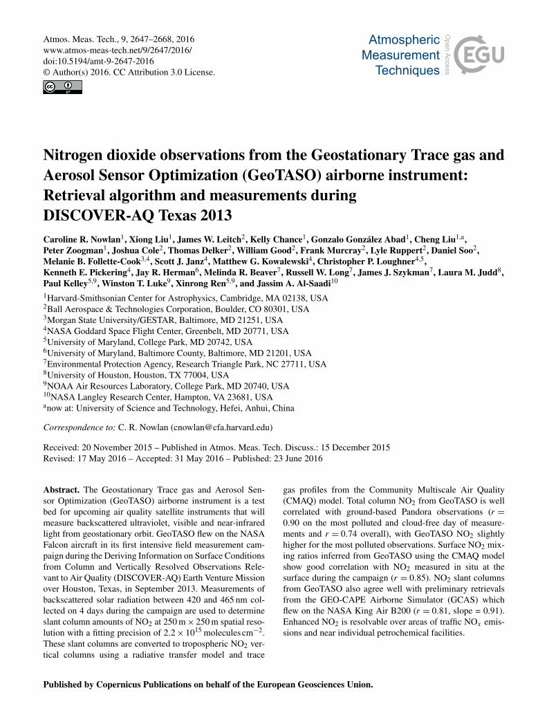
Abstract. The Geostationary Trace gas and Aerosol Sen-sor Optimization (GeoTASO) airborne instrument is a testbed for upcoming air quality satellite instruments that willmeasure backscattered ultraviolet, visible and near-infraredlight from geostationary orbit. GeoTASO flew on the NASAFalcon aircraft in its first intensive field measurement cam-paign during the Deriving Information on Surface Conditionsfrom Column and Vertically Resolved Observations Rele-vant to Air Quality (DISCOVER-AQ) Earth Venture Missionover Houston, Texas, in September 2013. Measurements ofbackscattered solar radiation between 420 and 465 nm col-lected on 4 days during the campaign are used to determineslant column amounts of NO2 at 250 m× 250 m spatial reso-lution with a fitting precision of 2.2× 10¹⁵ moleculescm−2.These slant columns are converted to tropospheric NO2 ver-tical columns using a radiative transfer model and trace
gas profiles from the Community Multiscale Air Quality(CMAQ) model. Total column NO2 from GeoTASO is wellcorrelated with ground-based Pandora observations (r =0.90 on the most polluted and cloud-free day of measure-ments and r = 0.74 overall), with GeoTASO NO2 slightlyhigher for the most polluted observations. Surface NO2 mix-ing ratios inferred from GeoTASO using the CMAQ modelshow good correlation with NO2 measured in situ at thesurface during the campaign (r = 0.85). NO2 slant columnsfrom GeoTASO also agree well with preliminary retrievalsfrom the GEO-CAPE Airborne Simulator (GCAS) whichflew on the NASA King Air B200 (r = 0.81, slope = 0.91).Enhanced NO2 is resolvable over areas of traffic NOx emis-sions and near individual petrochemical facilities.
Published by Copernicus Publications on behalf of the European Geosciences Union.
2648 C. R. Nowlan et al.: NO2 retrievals from GeoTASO
1 Introduction
The next generation of satellite instruments designed for airquality applications will operate from geostationary orbit,providing measurements of trace gases in the Earth’s at-mosphere with unprecedented spatial and temporal resolu-tion. These instruments include the upcoming TroposphericEmissions: Monitoring of POllution (TEMPO) instrument(Chance et al., 2013), which is a component of the NASAdecadal survey mission GEOstationary Coastal and Air Pol-lution Events (GEO-CAPE) (Fishman et al., 2012), the Geo-stationary Environmental Monitoring Spectrometer (GEMS)(Kim, 2012) and the Sentinel-4 mission (Ingmann et al.,2012), which will focus respectively on North America, EastAsia, and Europe and North Africa.
One of the principal trace gas products of these instru-ments is nitrogen dioxide (NO2). Nitrogen oxides (NOx ≡NO+NO2) play a central role in atmospheric air quality. NO2is a toxic gas, and NOx is involved in aerosol production andozone photochemistry. Globally, the major sources of NOxare combustion (primarily from transportation and thermalpower plants), soils and lightning. In urban areas, sources ofNOx are dominated by transportation and industry, with NO2showing a strong correlation with total population (Lamsalet al., 2013).
NO2 has relatively strong spectral absorption features inthe visible region of the spectrum, which have been exploitedover the past 2 decades for remote sensing using measure-ments of backscattered solar radiation from several instru-ments on sun-synchronous satellites (Martin et al., 2002;Boersma et al., 2004; Richter et al., 2011; Bucsela et al.,2013). These instruments are the predecessors of the upcom-ing geostationary air quality instruments.
The Geostationary Trace gas and Aerosol Sensor Opti-mization (GeoTASO) aircraft instrument (Leitch et al., 2014)has been developed by Ball Aerospace under the NASAEarth Science Technology Office Instrument Incubator Pro-gram in support of satellite measurements from geostation-ary orbit. Originally conceived as a test bed instrument forGEO-CAPE, GeoTASO is now also part of the mission riskreduction for TEMPO and GEMS in both instrument designand retrieval algorithm development.
GeoTASO is able to map the atmosphere in two dimen-sions (2-D) under the aircraft’s flight track. GeoTASO oper-ates as a hyperspectral push broom scanner, where the spec-tral information is provided by the y dimension of a 2-Dcharge-coupled device (CCD) array detector, the cross-trackspatial dimension is provided by the x dimension of the ar-ray and the along-track spatial dimension is provided by themovement of the aircraft in its flight path. Pushbroom scan-ner measurements are analogous to the type of measurementsthat will be made by the geostationary satellite instruments,but the satellite instruments will utilize a scan mirror to movethe field of view (FOV).
These types of measurements from aircraft are relativelynew, with push broom NO2 airborne 2-D measurements re-ported recently over the Highveld region of South Africa(Heue et al., 2008), Zurich, Switzerland (Popp et al., 2012),northwest Germany (Schönhardt et al., 2015) and Leices-ter, United Kingdom (Lawrence et al., 2015). General et al.(2014) have also recently reported airborne 2-D observa-tions of volcanic BrO and SO2 over Mt. Etna, BrO and NO2over Alaska and NO2 over Indianapolis using an instrumentequipped with a whisk broom scanner for nadir observationsand a push broom scanner observing in limb geometry forobtaining vertical information. In addition, the GEO-CAPEAirborne Simulator (GCAS) (Kowalewski and Janz, 2014) isa recently developed push broom sensor which had its firstcampaign deployment at the same time as GeoTASO.
This paper introduces the GeoTASO instrument and de-scribes algorithm development and the first trace gas re-trievals of NO2 from this new instrument. Section 2 describesthe GeoTASO optical design and measurement strategy. Sec-tion 3 describes the deployment of GeoTASO during theDeriving Information on Surface Conditions from Columnand Vertically Resolved Observations Relevant to Air Qual-ity (DISCOVER-AQ) Texas 2013 field campaign and intro-duces supporting measurements for validation. Section 4 de-scribes the data analysis for GeoTASO observations includ-ing calibration and spectral fitting for the retrieval of trace gasamounts. Section 5 presents the first results from GeoTASOand validation using data from other instruments collectedduring the DISCOVER-AQ campaign. Section 6 summarizesthe current status of GeoTASO and presents plans for futuredata analysis.
2 GeoTASO instrument
GeoTASO (Leitch et al., 2014) is a hyperspectral instrumentmeasuring nadir backscattered light in the ultraviolet and vis-ible in two channels at wavelengths 290–400 (UV) and 415–695 nm (VIS). Table 1 summarizes the main characteristicsof the instrument.
2.1 Spectrometer design
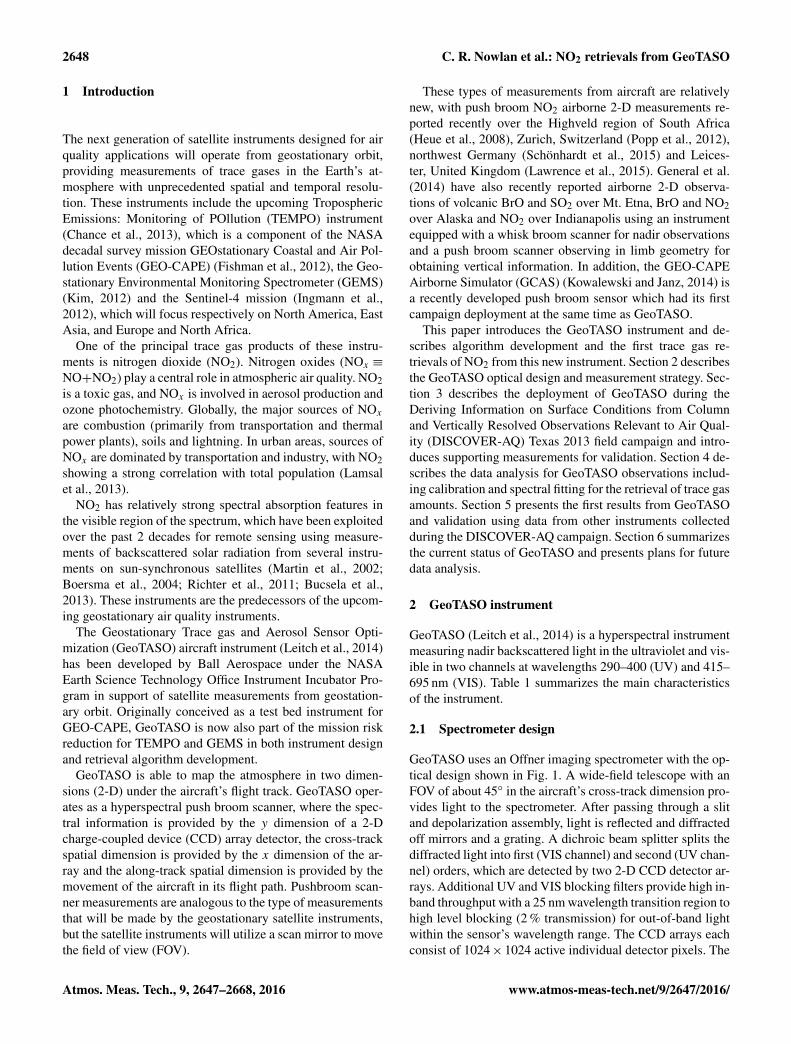
GeoTASO uses an Offner imaging spectrometer with the op-tical design shown in Fig. 1. A wide-field telescope with anFOV of about 45◦ in the aircraft’s cross-track dimension pro-vides light to the spectrometer. After passing through a slitand depolarization assembly, light is reflected and diffractedoff mirrors and a grating. A dichroic beam splitter splits thediffracted light into first (VIS channel) and second (UV chan-nel) orders, which are detected by two 2-D CCD detector ar-rays. Additional UV and VIS blocking filters provide high in-band throughput with a 25 nm wavelength transition region tohigh level blocking (2 % transmission) for out-of-band lightwithin the sensor’s wavelength range. The CCD arrays eachconsist of 1024× 1024 active individual detector pixels. The
C. R. Nowlan et al.: NO2 retrievals from GeoTASO 2649
Table 1. GeoTASO instrument characteristics. Four different slit sizes can be used in a slit holder assembly to give different spectral resolu-tions and spectral sampling values.
Figure 1. GeoTASO spectrometer design. First and second diffrac-tion orders are separated into Vis and UV channels by the beamsplitter and filters.
slit image is slightly smaller than the full array to allow forslight image shifting and to facilitate initial alignment, so thatonly the central 975 pixels in the cross-track dimension arewell illuminated in nadir observations. In the wavelength di-mension, the image covers 740 pixels on the UV detector and1000 pixels on the visible detector. The spectral sampling is0.14 nm for the UV and 0.28 nm for the visible detector.
The GeoTASO instrument design uses a reconfigurableslit and depolarization assembly for testing the sensitivityof trace gas retrievals to changing passband, spectral sam-pling and polarization. The 13 mm long slit can be replacedmanually, in a precision-registered slit holder that maintainsinstrument alignment, by slits of various widths (26.0, 32.5,39.0 and 45.5 µm). Under microscope testing, slit edges werefree of pronounced jaggedness at high spectral frequencies,and were uniform in width to at least ±2 µm, the limit of themicroscope setup. A pair of electronically controlled photoe-lastic modulators (PEMs) positioned before and after the slitserve as a depolarizer (Illing, 2009) that can be turned offand on or adjusted to optimize depolarization at particularwavelengths during the flight. These are flat parallel windows
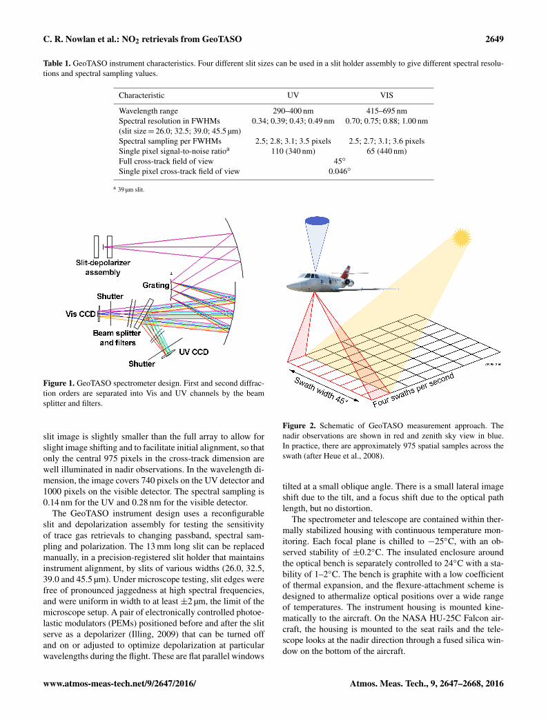
Figure 2. Schematic of GeoTASO measurement approach. Thenadir observations are shown in red and zenith sky view in blue.In practice, there are approximately 975 spatial samples across theswath (after Heue et al., 2008).
tilted at a small oblique angle. There is a small lateral imageshift due to the tilt, and a focus shift due to the optical pathlength, but no distortion.
The spectrometer and telescope are contained within ther-mally stabilized housing with continuous temperature mon-itoring. Each focal plane is chilled to −25◦C, with an ob-served stability of ±0.2◦C. The insulated enclosure aroundthe optical bench is separately controlled to 24◦C with a sta-bility of 1–2◦C. The bench is graphite with a low coefficientof thermal expansion, and the flexure-attachment scheme isdesigned to athermalize optical positions over a wide rangeof temperatures. The instrument housing is mounted kine-matically to the aircraft. On the NASA HU-25C Falcon air-craft, the housing is mounted to the seat rails and the tele-scope looks at the nadir direction through a fused silica win-dow on the bottom of the aircraft.
2650 C. R. Nowlan et al.: NO2 retrievals from GeoTASO
2.2 Measurement strategy
Figure 2 shows the geometry of the GeoTASO observations.At a typical flight altitude of 11 km above the surface, the 45◦
FOV results in a cross-track FOV of 9.1 km for the full field.This results in a cross-track instantaneous FOV (IFOV) of ap-proximately 9 m for each spatial sample. The 1.2 mrad along-track IFOV (39 µm slit) projects to an along-track IFOV of13–15 m at the ground. The along-track FOV is furthermoredetermined by the product of the detector integration timeof 0.25 s and the aircraft ground speed, with some varia-tion due to aircraft pitch. At typical aircraft ground speed(∼ 200 ms−1) and pitch, the along-track FOV is on the orderof 50–80 m.
Nadir measurements are typically interspersed with manu-ally commanded zenith sky reference and dark current obser-vations. GeoTASO collects zenith observations through anoptical fiber bundle that looks out the top of the aircraft. Asa result, the zenith spectra fill only the center of the FOVand are detected with sufficient signal for analysis over about60 pixels in the cross-track dimension. A typical zenith-sky measurement sequence collects about 580 such obser-vations, resulting in approximately 35 000 individual spectraper zenith sequence. Zenith sky spectra are co-added to im-prove the signal-to-noise ratio as described in Sect. 4.2. Darkcurrent observations are also collected periodically by com-manding the closure of shutters immediately in front of theCCD arrays.
3 DISCOVER-AQ campaign
DISCOVER-AQ was a NASA Earth Venture suborbital classmission which involved four field campaigns over 4 years,aimed at improving the ability of satellite observations tobe applied for air quality monitoring (http://discover-aq.larc.nasa.gov/). As part of the campaigns, instruments on theNASA King Air B200 aircraft (remote sensing observations)and the P-3B aircraft (in situ observations) collected a largesuite of trace gas, meteorological and aerosol observations inconcert with stationary and mobile ground-based and ship-based remote sensing and in situ monitoring instruments.GeoTASO flew on the NASA HU-25C Falcon aircraft dur-ing the DISCOVER-AQ field campaigns in September 2013(Texas) and July–August 2014 (Colorado).
3.1 GeoTASO measurements during DISCOVER-AQTexas 2013
During the 2013 campaign, the GeoTASO instrument wasbased in southeast Houston at the William P. Hobby Air-port and flew seven flights on 6 days between 12 and 24September 2013, including inbound and outbound transitsfrom and to the Falcon’s base at NASA Langley ResearchCenter in Virginia. Table 2 summarizes these flights, alongwith the slit size used for each flight. The inbound transit
from Virginia included observations near Atlanta, Georgia,close to large power plants. The 16 September flight made adirect underpass of the Aura satellite as it passed over south-ern Oklahoma. This flight was made with the intention tocompare with retrievals from the Ozone Monitoring Instru-ment (OMI) on Aura; although OMI NO2 measurements onthat day over Texas and Oklahoma were below the detectionlimit, GeoTASO was able to detect NO2 over Forth Worth,Texas. The 17 September observations were made primar-ily over water, in support of the ocean color segment of theGEO-CAPE mission, which aims to derive chlorophyll fluo-rescence and water-leaving radiances in the near-UV, visibleand near-infrared from geostationary orbit. The 13, 14, 18and 24 (Leg 1) September flights occurred over the greaterHouston area and enabled observations of pollution from in-dustrial and urban transportation sources. Leg 2 of the 24September flights passed over three large power plants inNorth Carolina during the aircraft’s transit back to Virginia.In this paper, we examine data from the Houston urban flightson 13, 14, 18 and 24 September.
3.2 Additional data sources
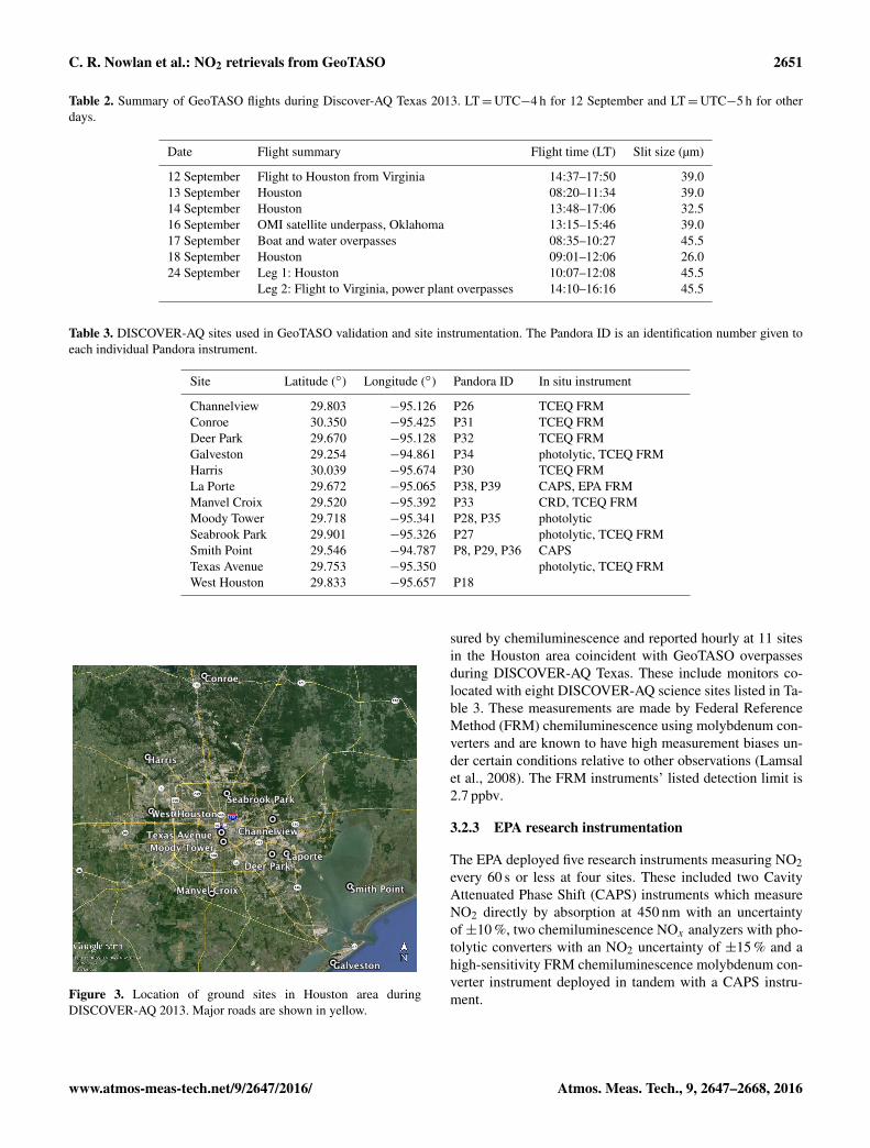
In this study, we use NO2 data from ground, aircraft andsatellite-based measurements, as well as model data pro-duced for the campaign. The surface observations are primar-ily from 12 DISCOVER-AQ campaign sites in the Houstonarea, which are listed in Table 3 along with the instrumentsdeployed at the sites. Figure 3 shows the location of theseDISCOVER-AQ sites.
3.2.1 Pandora
Total column NO2 was measured by Pandora spectrometers(Herman et al., 2009) during DISCOVER-AQ Texas by di-rect sun observation with a temporal resolution of 90 s, a typ-ical precision of 2.7× 10¹⁴ moleculescm−2 and an accuracyof 2.7× 10¹⁵ moleculescm−2. Pandora NO2 is determinedfrom the difference between the direct sun observation anda reference spectrum derived using clean observations on aclear day. Total column NO2 is derived using NO2 cross sec-tions from Vandaele et al. (1998) at an effective temperatureof 250 K derived from NO2 and temperature profiles as de-scribed in Herman et al. (2009). We use column NO2 datafrom 15 Pandora instruments deployed at 11 sites coincidentwith GeoTASO overpasses.
3.2.2 TCEQ SLAMS
The Environmental Protection Agency (EPA) coordinates aseries of sites as part of the national State and Local AirMonitoring Stations (SLAMS) and relevant air quality net-works which monitor ambient air quality in the United Statesat rural, suburban and urban locations. In Texas, these are op-erated by the Texas Commission on Environmental Quality(TCEQ). We use TCEQ SLAMS NO2 measurements mea-
C. R. Nowlan et al.: NO2 retrievals from GeoTASO 2651
Table 2. Summary of GeoTASO flights during Discover-AQ Texas 2013. LT=UTC−4 h for 12 September and LT=UTC−5 h for otherdays.
Date Flight summary Flight time (LT) Slit size (µm)
12 September Flight to Houston from Virginia 14:37–17:50 39.013 September Houston 08:20–11:34 39.014 September Houston 13:48–17:06 32.516 September OMI satellite underpass, Oklahoma 13:15–15:46 39.017 September Boat and water overpasses 08:35–10:27 45.518 September Houston 09:01–12:06 26.024 September Leg 1: Houston 10:07–12:08 45.5
Leg 2: Flight to Virginia, power plant overpasses 14:10–16:16 45.5
Table 3. DISCOVER-AQ sites used in GeoTASO validation and site instrumentation. The Pandora ID is an identification number given toeach individual Pandora instrument.
Site Latitude (◦) Longitude (◦) Pandora ID In situ instrument
Figure 3. Location of ground sites in Houston area duringDISCOVER-AQ 2013. Major roads are shown in yellow.
sured by chemiluminescence and reported hourly at 11 sitesin the Houston area coincident with GeoTASO overpassesduring DISCOVER-AQ Texas. These include monitors co-located with eight DISCOVER-AQ science sites listed in Ta-ble 3. These measurements are made by Federal ReferenceMethod (FRM) chemiluminescence using molybdenum con-verters and are known to have high measurement biases un-der certain conditions relative to other observations (Lamsalet al., 2008). The FRM instruments’ listed detection limit is2.7 ppbv.
3.2.3 EPA research instrumentation
The EPA deployed five research instruments measuring NO2every 60 s or less at four sites. These included two CavityAttenuated Phase Shift (CAPS) instruments which measureNO2 directly by absorption at 450 nm with an uncertaintyof ±10 %, two chemiluminescence NOx analyzers with pho-tolytic converters with an NO2 uncertainty of ±15 % and ahigh-sensitivity FRM chemiluminescence molybdenum con-verter instrument deployed in tandem with a CAPS instru-ment.
2652 C. R. Nowlan et al.: NO2 retrievals from GeoTASO
3.2.4 NOAA instrumentation
A cavity ring-down (CRD) instrument was deployed by theNational Oceanic and Atmospheric Administration (NOAA)and University of Maryland at the Manvel Croix science sitein the south of Houston. The CRD instrument measured am-bient NO2 every 10 s with an uncertainty of ±5 %. The in-strument was calibrated with a NIST-traceable NO2 standardas well as the gas-phase titration method (Brent et al., 2013).A NOAA chemiluminescence photolytic converter monitorwas also deployed at the Galveston site and reported mea-surements every 60 s, with an uncertainty of ±10 %.
3.2.5 University of Houston instrumentation
The University of Houston made measurements of NO2 at al-titudes of 7 and 70 m at the Moody Tower site in downtownHouston. These were collected with a chemiluminescencemonitor fitted with a photolytic converter and have a reporteduncertainty of ±12 %. Data are reported every 5 min.
3.2.6 GCAS
The GCAS instrument (Kowalewski and Janz, 2014) was de-ployed on the NASA King Air B200 aircraft as part of thecampaign’s airborne remote sensing payload, which also in-cluded the NASA High Spectral Resolution Lidar (HSRL)instrument (Hair et al., 2008) for aerosol studies. GCAS op-erates in a similar fashion to GeoTASO, using a 2-D CCD ar-ray detector to map slant columns of NO2 in two dimensions.The instrument uses an Offner imaging spectrometer withtwo 1072×1024 (spectral×spatial) pixel detector arrays inthe UV/visible (300–490 nm) and visible/near-infrared (480–900 nm). The UV/visible channel used for NO2 retrievalshas a spectral sampling of 0.2 nm and a spectral resolutionof 0.57 nm. The full cross-track FOV covers 45◦. At wave-length 440 nm and at a spatial resolution of 250m× 500m,the signal-to-noise ratio is on the order of 540. GCAS isa successor to the Airborne Compact Atmospheric Mapper(ACAM) scanning instrument (Liu et al., 2015) and flew inits first campaign deployment during DISCOVER-AQ Texas.
3.2.7 GOME-2
The Global Ozone Monitoring Experiment-2 (GOME-2) in-struments (Munro et al., 2016) were launched on the EU-METSAT satellites Metop-A in 2006 and Metop-B in 2013.GOME-2 instruments make nadir observations of backscat-tered solar radiation from 240 to 790 nm. Only Metop-Adata are considered here, as there were no cloud-free coin-cidences with Metop-B during DISCOVER-AQ Texas. Asof mid-2013, the GOME-2/Metop-A nominal pixel resolu-tion is 40× 40 km2. We use the publicly available BIRA-IASB/KNMI GOME-2 NO2 product TM4NO2A version 2.3(http://www.temis.nl) (Boersma et al., 2004).
Figure 4. 36, 12 and 4 km CMAQ modeling domains.
3.2.8 CMAQ model
The EPA’s Community Multiscale Air Quality (CMAQ) ver-sion 5.0.2 modeling system (Byun and Schere, 2006) wasused to simulate air quality from 18 August 2013 through 1October 2013. CMAQ used offline meteorology from the Ad-vanced Research Weather Research and Forecasting (WRF-ARW) model (Skamarock et al., 2008) via the Meteorology–Chemistry Interface Processor (MCIP) (Otte and Pleim,2010). This time period covers the entire DISCOVER-AQTexas field deployment in September 2013 plus additionaldays in August to provide adequate model spin-up time. TheCMAQ model simulations used in the GeoTASO analysishave a spatial resolution of 4× 4 km2 and a temporal reso-lution of 20 min. The local bay and sea breezes that affectair quality in this region are best simulated at the high res-olutions of a regional model over those available from mostglobal models. We apply CMAQ and WRF due to previoussuccess capturing local-scale bay and sea breezes with thesemodels (Loughner et al., 2011).
Figure 4 shows the 36, 12 and 4 km modeling domains.The 12 km North American Mesoscale (NAM) model wasused for meteorological initial and boundary conditions.Observational and analysis nudging were performed on alldomains. Observational nudging was done using the Na-tional Centers for Environmental Prediction (NCEP) Auto-mated Data Processing (ADP) Global Surface (http://rda.ucar.edu/datasets/ds461.0/) and Upper Air (http://rda.ucar.edu/datasets/ds351.0/) Observational Weather Data.
WRF was run using an iterative technique developed atthe EPA (Appel et al., 2014). The initial WRF run performedanalysis nudging on all domains based on the 12 km NAM.The second WRF run performed analysis nudging on all do-mains based on the 12 km NAM except for 2 m temperatureand humidity for the 4 km domain, for which 2 m temper-ature and humidity from the 4 km initial WRF simulationwere used for nudging. This modeling technique prevented
Biogenic (BEIS) and lightning emissions calculated within CMAQInitial and boundary conditions MOZART CTM
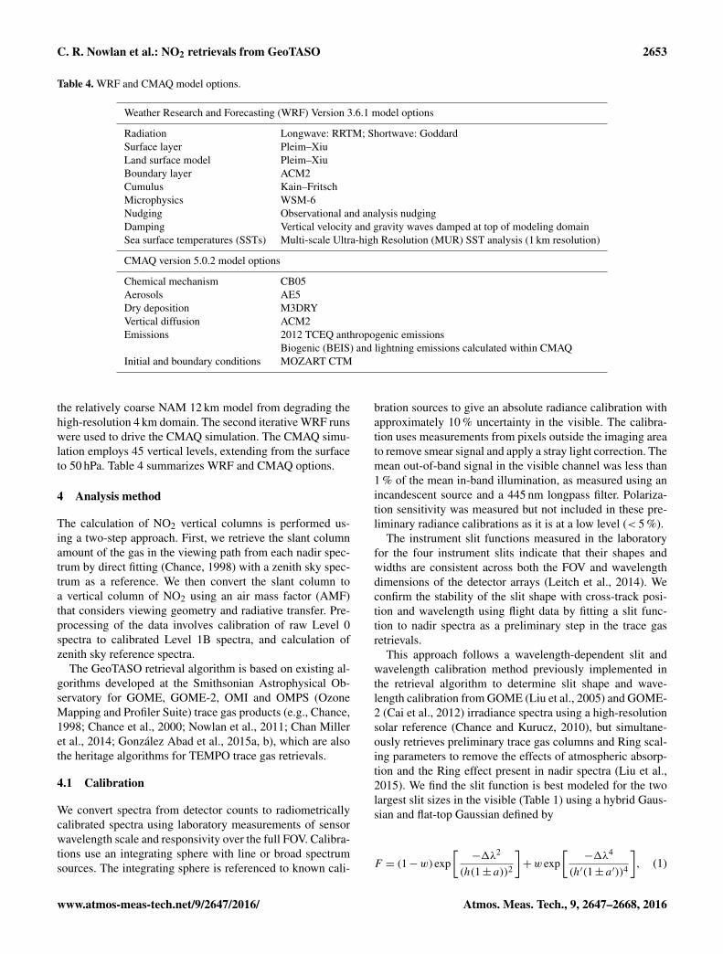
the relatively coarse NAM 12 km model from degrading thehigh-resolution 4 km domain. The second iterative WRF runswere used to drive the CMAQ simulation. The CMAQ simu-lation employs 45 vertical levels, extending from the surfaceto 50 hPa. Table 4 summarizes WRF and CMAQ options.
4 Analysis method
The calculation of NO2 vertical columns is performed us-ing a two-step approach. First, we retrieve the slant columnamount of the gas in the viewing path from each nadir spec-trum by direct fitting (Chance, 1998) with a zenith sky spec-trum as a reference. We then convert the slant column toa vertical column of NO2 using an air mass factor (AMF)that considers viewing geometry and radiative transfer. Pre-processing of the data involves calibration of raw Level 0spectra to calibrated Level 1B spectra, and calculation ofzenith sky reference spectra.
The GeoTASO retrieval algorithm is based on existing al-gorithms developed at the Smithsonian Astrophysical Ob-servatory for GOME, GOME-2, OMI and OMPS (OzoneMapping and Profiler Suite) trace gas products (e.g., Chance,1998; Chance et al., 2000; Nowlan et al., 2011; Chan Milleret al., 2014; González Abad et al., 2015a, b), which are alsothe heritage algorithms for TEMPO trace gas retrievals.
4.1 Calibration
We convert spectra from detector counts to radiometricallycalibrated spectra using laboratory measurements of sensorwavelength scale and responsivity over the full FOV. Calibra-tions use an integrating sphere with line or broad spectrumsources. The integrating sphere is referenced to known cali-
bration sources to give an absolute radiance calibration withapproximately 10 % uncertainty in the visible. The calibra-tion uses measurements from pixels outside the imaging areato remove smear signal and apply a stray light correction. Themean out-of-band signal in the visible channel was less than1 % of the mean in-band illumination, as measured using anincandescent source and a 445 nm longpass filter. Polariza-tion sensitivity was measured but not included in these pre-liminary radiance calibrations as it is at a low level (< 5 %).
The instrument slit functions measured in the laboratoryfor the four instrument slits indicate that their shapes andwidths are consistent across both the FOV and wavelengthdimensions of the detector arrays (Leitch et al., 2014). Weconfirm the stability of the slit shape with cross-track posi-tion and wavelength using flight data by fitting a slit func-tion to nadir spectra as a preliminary step in the trace gasretrievals.
This approach follows a wavelength-dependent slit andwavelength calibration method previously implemented inthe retrieval algorithm to determine slit shape and wave-length calibration from GOME (Liu et al., 2005) and GOME-2 (Cai et al., 2012) irradiance spectra using a high-resolutionsolar reference (Chance and Kurucz, 2010), but simultane-ously retrieves preliminary trace gas columns and Ring scal-ing parameters to remove the effects of atmospheric absorp-tion and the Ring effect present in nadir spectra (Liu et al.,2015). We find the slit function is best modeled for the twolargest slit sizes in the visible (Table 1) using a hybrid Gaus-sian and flat-top Gaussian defined by
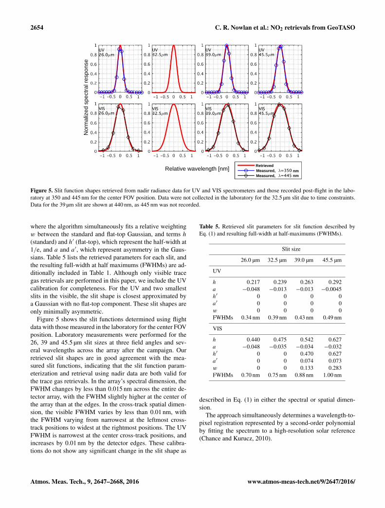
Figure 5. Slit function shapes retrieved from nadir radiance data for UV and VIS spectrometers and those recorded post-flight in the labo-ratory at 350 and 445 nm for the center FOV position. Data were not collected in the laboratory for the 32.5 µm slit due to time constraints.Data for the 39 µm slit are shown at 440 nm, as 445 nm was not recorded.
where the algorithm simultaneously fits a relative weightingw between the standard and flat-top Gaussian, and terms h(standard) and h′ (flat-top), which represent the half-width at1/e, and a and a′, which represent asymmetry in the Gaus-sians. Table 5 lists the retrieved parameters for each slit, andthe resulting full-width at half maximums (FWHMs) are ad-ditionally included in Table 1. Although only visible tracegas retrievals are performed in this paper, we include the UVcalibration for completeness. For the UV and two smallestslits in the visible, the slit shape is closest approximated bya Gaussian with no flat-top component. These slit shapes areonly minimally asymmetric.
Figure 5 shows the slit functions determined using flightdata with those measured in the laboratory for the center FOVposition. Laboratory measurements were performed for the26, 39 and 45.5 µm slit sizes at three field angles and sev-eral wavelengths across the array after the campaign. Ourretrieved slit shapes are in good agreement with the mea-sured slit functions, indicating that the slit function param-eterization and retrieval using nadir data are both valid forthe trace gas retrievals. In the array’s spectral dimension, theFWHM changes by less than 0.015 nm across the entire de-tector array, with the FWHM slightly higher at the center ofthe array than at the edges. In the cross-track spatial dimen-sion, the visible FWHM varies by less than 0.01 nm, withthe FWHM varying from narrowest at the leftmost cross-track positions to widest at the rightmost positions. The UVFWHM is narrowest at the center cross-track positions, andincreases by 0.01 nm by the detector edges. These calibra-tions do not show any significant change in the slit shape as
Table 5. Retrieved slit parameters for slit function described byEq. (1) and resulting full-width at half-maximums (FWHMs).
described in Eq. (1) in either the spectral or spatial dimen-sion.
The approach simultaneously determines a wavelength-to-pixel registration represented by a second-order polynomialby fitting the spectrum to a high-resolution solar reference(Chance and Kurucz, 2010).
C. R. Nowlan et al.: NO2 retrievals from GeoTASO 2655
4.2 Zenith sky reference spectra
We determine a mean zenith sky reference spectrum foreach nadir observation using the nearest three zenith sky se-quences closest in time, which usually occur within 20 min ofthe nadir observation. The signal-to-noise ratio of the result-ing zenith spectrum varies with solar zenith angle and wave-length, but is approximately 1000–2000 in the NO2 fittingwindow. In future, averaging could include even more spec-tra to reduce the influence of zenith noise in the retrievals.
4.3 Spectral fitting
We determine NO2 slant columns from individual spectraat native spatial resolution between wavelengths 420 and465 nm by simultaneously fitting line-of-sight NO2 slantcolumns and other parameters listed in Table 6.
The fit includes molecular absorbers NO2, O3, H2O va-por and O2–O2, as well as the following pseudo-absorbers: aRing spectrum that accounts for filling-in of Fraunhofer linesin the solar spectrum due to rotational Raman scattering; un-dersampling of the spectrum that occurs when spectral sam-pling is less than∼ 3 pixels across the FWHM (Chance et al.,2005), which is necessary for the 26 and 32.5 µm slit sizeswhere sampling is 2.5 and 2.7 pixels/FWHM, respectively;and baseline (fourth order) and scaling (fifth order) polyno-mials to represent low frequency features in the spectrumdue to aerosols, molecular scattering, wavelength-dependentalbedo and low-order effects that may not be accounted forproperly in radiometric calibration. A wavelength shift isalso fit to account for the relative difference in wavelength-detector pixel registration between the nadir radiance and ref-erence spectra.
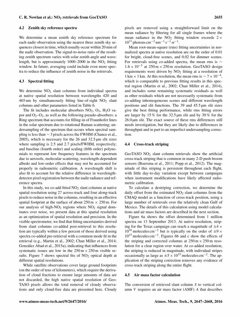
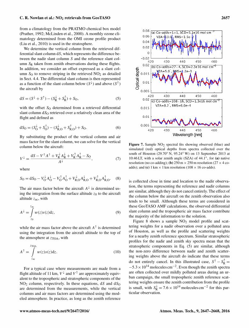
In this study, we co-add fitted NO2 slant columns at nativespatial resolution using 27 across-track and four along-trackpixels to reduce noise in the columns, resulting in an effectivespatial footprint at the surface of about 250 m × 250 m. Forour analysis of high-NO2 regions where NO2 signal dom-inates over noise, we present data at this spatial resolutionas an optimization of spatial resolution and precision. In thevisible spectrometer, we find that fitting uncertainties derivedfrom slant columns co-added post-retrieval to this resolu-tion are typically within a few percent of those derived usingspectra co-added pre-retrieval with a common mode fit in theretrieval (e.g., Martin et al., 2002; Chan Miller et al., 2014;González Abad et al., 2015a), indicating that influences fromsystematic issues are low in the 250 m× 250 m visible re-sults. Figure 7 shows spectral fits of NO2 optical depth atdifferent spatial resolutions.
While satellite observations cover large ground footprints(on the order of tens of kilometers), which require the deriva-tion of cloud fractions to ensure large amounts of data arenot discarded, the high native spatial resolution of Geo-TASO pixels allows the total removal of cloudy observa-tions and only cloud-free data are presented here. Cloudy
pixels are removed using a straightforward limit on themean radiance by filtering for all single frames where themean radiance in the NO2 fitting window exceeds 2×10¹³ photonscm−2 nm−1 s−1 sr−1.
Mean root-mean-square (rms) fitting uncertainties in nor-malized spectra at native resolution are on the order of 0.01for bright, cloud-free scenes, and 0.02 for dimmer scenes.For retrievals using co-added spectra, the mean rms is ∼1.6× 10⁻³ at 250 m× 250 m resolution. GeoTASO designrequirements were driven by NO2 fitting at a resolution of1 km× 1 km. At this resolution, the mean rms is ∼ 7×10⁻⁴,which is comparable to previous fitting results in this spec-tral region (Martin et al., 2002; Chan Miller et al., 2014),and includes some remaining systematic residuals as wellas other residuals which are not necessarily systematic fromco-adding inhomogeneous scenes and different wavelengthpositions and slit functions. The 39 and 45.5 µm slit sizesgive the best fitting performance, while rms fitting errorsare larger by 15 % for the 32.5 µm slit and by 30 % for the26.0 µm slit. The exact source of these rms differences stillneeds investigation, but they are likely due to differences inthroughput and in part to an imperfect undersampling correc-tion.
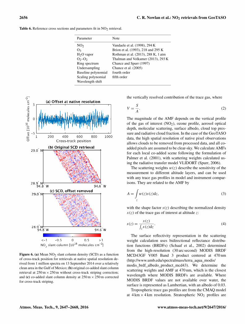
4.4 Cross-track striping
GeoTASO NO2 slant column retrievals show the artificialcross-track striping that is common in many 2-D push broomsensors (Boersma et al., 2011; Popp et al., 2012). The mag-nitude of this striping is persistent throughout each flight,with little day-to-day variation except between campaignswhen instrument modifications have likely affected radio-metric calibration.
To calculate a destriping correction, we determine thedaily offset from the estimated NO2 slant columns from theCMAQ model as a function of cross-track position, using alarge number of retrievals over the relatively clean Gulf ofMexico. The details of this calculation using model calcula-tions and air mass factors are described in the next section.
Figure 6a shows the offset determined from 1 millionspectra on 13 September 2013. At native resolution, strip-ing for the Texas campaign can reach a magnitude of ±4×10¹⁶ moleculescm−2 but is typically on the order of ±9×10¹⁵ moleculescm−2. Figures 6b and c show the effects ofthe striping and corrected columns at 250 m× 250 m reso-lution for a clear region over water. At co-added resolution,the striping is reduced in magnitude, with individual stripesoccasionally as large as ±5× 10¹⁵ moleculescm−2. The ap-plication of the striping correction removes any evidence ofcross-track striping along the entire flight.
4.5 Air mass factor calculation
The conversion of retrieved slant column S to vertical col-umn V requires an air mass factor (AMF) A that describes
2656 C. R. Nowlan et al.: NO2 retrievals from GeoTASO
Table 6. Reference cross sections and parameters fit in NO2 retrieval.
Parameter Note
NO2 Vandaele et al. (1998), 294 KO3 Brion et al. (1993), 218 and 295 KH2O vapor Rothman et al. (2013), 288 K, 1 atmO2–O2 Thalman and Volkamer (2013), 293 KRing spectrum Chance and Spurr (1997)Undersampling Chance et al. (2005)Baseline polynomial fourth orderScaling polynomial fifth orderWavelength shift
Figure 6. (a) Mean NO2 slant column density (SCD) as a functionof cross-track position for retrievals at native spatial resolution de-rived from 1 million spectra on 13 September 2014 over a relativelyclean area in the Gulf of Mexico; (b) original co-added slant columnretrieval at 250 m× 250 m without cross-track striping correction;and (c) co-added slant column density at 250 m× 250 m correctedfor cross-track striping.
the vertically resolved contribution of the trace gas, where
V =S
A. (2)
The magnitude of the AMF depends on the vertical profileof the gas of interest (NO2), ozone profile, aerosol opticaldepth, molecular scattering, surface albedo, cloud top pres-sure and radiative cloud fraction. In the case of the GeoTASOdata, the high spatial resolution of native pixel observationsallows clouds to be removed from processed data, and all co-added pixels are assumed to be clear-sky. We calculate AMFsfor each local co-added scene following the formulation ofPalmer et al. (2001), with scattering weights calculated us-ing the radiative transfer model VLIDORT (Spurr, 2006).
The scattering weights w(z) describe the sensitivity of themeasurement to different altitude layers, and can be usedwith any trace gas profiles in model and instrument compar-isons. They are related to the AMF by
A=
∫z
w(z)s(z)dz, (3)
with the shape factor s(z) describing the normalized densityx(z) of the trace gas of interest at altitude z:
s(z)=x(z)∫zx(z)dz
. (4)
The surface reflectivity representation in the scatteringweight calculation uses bidirectional reflectance distribu-tion functions (BRDFs) (Schaaf et al., 2002) determinedfrom the high-resolution (30 arc second) MODIS BRDFMCD43GF V005 Band 3 product centered at 470 nm(http://www.umb.edu/spectralmass/terra_aqua_modis/modis_brdf_albedo_product_mcd43). We determine thescattering weights and AMF at 470 nm, which is the closestwavelength where MODIS BRDFs are available. WhereMODIS BRDF values are not available over water, thesurface is represented as Lambertian, with an albedo of 0.03.
Tropospheric trace gas profiles are from the CMAQ modelat 4 km× 4 km resolution. Stratospheric NO2 profiles are
C. R. Nowlan et al.: NO2 retrievals from GeoTASO 2657
from a climatology from the PRATMO chemical box model(Prather, 1992; McLinden et al., 2000). A monthly ozone cli-matology determined from the OMI ozone profile product(Liu et al., 2010) is used in the stratosphere.
We determine the vertical column from the retrieved dif-ferential slant column dS, which represents the difference be-tween the nadir slant column S and the reference slant col-umn SR taken from zenith observations during these flights.In addition, we consider an offset expressed as a slant col-umn SO to remove striping in the retrieved NO2 as detailedin Sect. 4.4. The differential slant column is then representedas a function of the slant column below (S↓) and above (S↑)the aircraft by
dS = (S↓+ S↑)− (S↓R + S↑
R)+ SO, (5)
with the offset SO determined from a retrieved differentialslant column dSO retrieved over a relatively clean area of theflight and defined as
dSO = (S↓
O+ S↑
O)− (S↓
R,O+ S↑
R,O)+ SO. (6)
By substituting the product of the vertical column and airmass factor for the slant column, we can solve for the verticalcolumn below the aircraft:
V ↓ =dS−V ↑A↑+V ↓RA
↓
R+V↑
RA↑
R− SO
A↓, (7)
where
SO = dSO−V↓
OA↓
O−V↑
OA↑
O+V↓
R,OA↓
R,O+V↑
R,OA↑
R,O. (8)
The air mass factor below the aircraft A↓ is determined us-ing the integration from the surface altitude z0 to the aircraftaltitude zac, with
A↓ =
zac∫z0
w(z)s(z)dz, (9)
while the air mass factor above the aircraft A↑ is determinedusing the integration from the aircraft altitude to the top ofthe atmosphere at zTOA, with
A↑ =
zTOA∫zac
w(z)s(z)dz. (10)
For a typical case where measurements are made from aflight altitude of 11 km, V ↓ and V ↑ are approximately equiv-alent to the tropospheric and stratospheric components of theNO2 column, respectively. In these equations, dS and dSOare determined from the measurements, while the verticalcolumns and air mass factors are determined using the mod-eled atmosphere. In practice, as long as the zenith reference
Figure 7. Sample NO2 spectral fits showing observed (blue) andsimulated (red) optical depths from spectra collected over thesouth of Houston (29.70◦ N, 95.24◦W) on 13 September 2013 at10:46 LT, with a solar zenith angle (SZA) of 44.1◦, for (a) nativeresolution (no co-adding); (b) 250 m× 250 m resolution (27× 4 co-adds); and (c) 1 km× 1 km resolution (108× 16 co-adds).
is collected close in time and location to the nadir observa-tion, the terms representing the reference and nadir columnsare similar, although they do not cancel entirely. The effect ofthe column below the aircraft on the zenith observation alsotends to be small. Although these terms are considered inthese GeoTASO AMF calculations, the observed differentialslant column and the tropospheric air mass factor contributethe majority of the information to the solution.
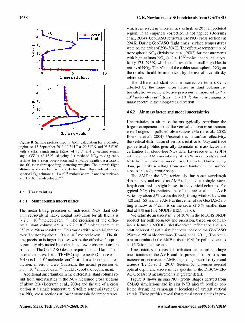
Figure 8 shows a sample NO2 model profile and scat-tering weights for a nadir observation over a polluted areaof Houston, as well as the profile and scattering weightsfor a nearby zenith reference spectrum. Similar stratosphericprofiles for the nadir and zenith sky spectra mean that thestratospheric components in Eq. (5) are similar, althoughthe non-zero difference between nadir and zenith scatter-ing weights above the aircraft do indicate that these termsdo not entirely cancel. In this illustrated case, S↑− S↑R =−5.3×10¹⁴ moleculescm−2. Even though the zenith spectraare often collected over mildly polluted areas during an ur-ban campaign, the small tropospheric zenith reference scat-tering weights ensure the zenith contribution from the profileis small, with S↓R = 7.6× 10¹⁴ moleculescm−2 for this par-ticular observation.
2658 C. R. Nowlan et al.: NO2 retrievals from GeoTASO
Figure 8. Sample profiles used in AMF calculation for a pollutedregion on 13 September 2013 10:31 LT at 29.51◦ N and 95.34◦W,with a solar zenith angle (SZA) of 47.0◦ and a viewing zenithangle (VZA) of 13.2◦, showing (a) modeled NO2 mixing ratioprofiles for a nadir observation and a nearby zenith observation;and (b) their corresponding scattering weights. The aircraft flightaltitude is shown by the black dashed line. The modeled tropo-spheric NO2 column is 1.1×10¹⁶ moleculescm−2 and the retrievedis 2.1× 10¹⁶ moleculescm−2.
4.6 Uncertainties
4.6.1 Slant column uncertainties
The mean fitting precision of individual NO2 slant col-umn retrievals at native spatial resolution for all flights is∼ 2.3× 10¹⁶ moleculescm−2. The precision of the differ-ential slant column dS is ∼ 2.2× 10¹⁵ moleculescm−2 at250 m× 250 m resolution. This varies with scene brightnessover Houston by about±0.4×10¹⁵ moleculescm−2. The fit-ting precision is larger in cases where the effective footprintis partially obstructed by a cloud and fewer observations areco-added. The GeoTASO design requirement at 1km× 1kmresolution derived from TEMPO requirements (Chance et al.,2013) is 1×10¹⁵ moleculescm−2; at 1km×1km spatial res-olution, if errors were Gaussian, the actual precision of5.5× 1014 moleculescm−2 could exceed the requirement.
Additional uncertainties in the differential slant column re-sult from uncertainties in the NO2 measured cross sectionsof about 2 % (Boersma et al., 2004) and the use of a crosssection at a single temperature. Satellite retrievals typicallyuse NO2 cross sections at lower stratospheric temperatures,
which can result in uncertainties as high as 20 % in pollutedregions if an empirical correction is not applied (Boersmaet al., 2004). GeoTASO retrievals use NO2 cross sections at294 K. During GeoTASO flight times, surface temperatureswere on the order of 296–304 K. The effective temperature oftropospheric NO2 (Brinksma et al., 2002) for measurementswith high column NO2 (> 3× 10¹⁵ moleculescm−2) is typ-ically 275–293 K, which could result in a small high bias inretrieved NO2. The effect of the colder stratospheric NO2 onthe results should be minimized by the use of a zenith skyreference.
The differential slant column correction term dSO isaffected by the same uncertainties in slant column re-trievals; however, its effective precision is improved to 7×10¹⁴ moleculescm−2 (rms= 5× 10⁻³) due to averaging ofmany spectra in the along-track direction.
4.6.2 Air mass factor and model uncertainties
Uncertainties in air mass factors typically contribute thelargest component of satellite vertical column measurementerror budgets in polluted observations (Martin et al., 2002;Boersma et al., 2004). Uncertainties in surface reflectivity,the vertical distribution of aerosols relative to NO2 and tracegas vertical profiles generally dominate air mass factor un-certainties for cloud-free NO2 data. Lawrence et al. (2015)estimated an AMF uncertainty of ∼ 8 % in remotely sensedNO2 from an airborne mission over Leicester, United King-dom, primarily resulting from uncertainties in the surfacealbedo and NO2 profile shape.
The AMF in the NO2 region also has some wavelengthdependency, and use of an AMF calculated at a single wave-length can lead to slight biases in the vertical columns. Fortypical NO2 observations, the effects are small; the AMFvaries by about 5 % across the NO2 fitting window between420 and 465 nm. The AMF at the center of the GeoTASO fit-ting window at 442 nm is on the order of 3 % smaller thanthat at 470 nm (the MODIS BRDF band).
We estimate an uncertainty of 20 % in the MODIS BRDFproduct for both accuracy and precision, based on compar-isons between MODIS BRDF-derived reflectance and air-craft observations at a similar spatial scale to the GeoTASO250m×250m observations (Román et al., 2011). The resul-tant uncertainty in the AMF is about 10 % for polluted scenesand 5 % for clean scenes.
Uncertainties in aerosol distribution can contribute largeuncertainties to the AMF, and the presence of aerosols canincrease or decrease the AMF, depending on aerosol type andaltitude (Leitão et al., 2010). Section 5.1 discusses aerosoloptical depth and uncertainties specific to the DISCOVER-AQ GeoTASO measurements in greater detail.
Figure 9 shows median NO2 profile shapes derived fromCMAQ simulations and in situ P-3B aircraft profiles col-lected during the campaign at locations of aircraft verticalspirals. These profiles reveal that typical uncertainties in pro-
C. R. Nowlan et al.: NO2 retrievals from GeoTASO 2659
Figure 9. Normalized median profile shapes from CMAQ modelsimulations and P-3B aircraft NO2 observations at P-3B spiral lo-cations during the DISCOVER-AQ Texas campaign. The profilesuse model output and observations binned to a 250 m altitude grid.
file shape factors are generally less than 20 %; uncertain-ties of this magnitude typically result in a ∼ 5 % uncertaintyin the AMF below the aircraft. Individual partial columnmodel uncertainties are sometimes much larger (>100 %)when compared with P-3B profiles, which can contribute asmall uncertainty through the term V
↓
R in Eq. (7). In addition,we estimate a 30 % uncertainty in NO2 stratospheric columnsfrom the PRATMO model, based on typical differences withOSIRIS limb measurements of NO2 (Bourassa et al., 2011).
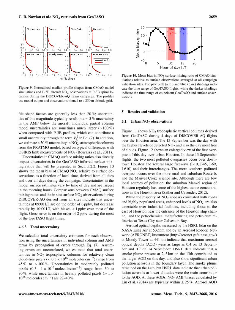
Uncertainties in CMAQ surface mixing ratios also directlyimpact uncertainties in the GeoTASO-inferred surface mix-ing ratios that will be presented in Sect. 5.2.2. Figure 10shows the mean bias of CMAQ NO2 relative to surface ob-servations as a function of local time, derived from all sitesand over all days during the campaign. Uncertainties in themodel surface estimates vary by time of day and are largestin the morning hours. Comparisons between CMAQ surfacemixing ratios and the in situ surface NO2 observations duringDISCOVER-AQ derived from all sites indicate that uncer-tainties at 09:00 LT are on the order of 6 ppbv, but decreaserapidly by 10:00 LT, with biases < 1 ppbv over most of theflight. Gross error is on the order of 2 ppbv during the mostof the GeoTASO flight times.
4.6.3 Total uncertainty
We calculate total uncertainty estimates for each observa-tion using the uncertainties in individual column and AMFterms by propagation of errors through Eq. (7). Assum-ing errors are uncorrelated, we estimate that total uncer-tainties in NO2 tropospheric columns for relatively cleancloud-free pixels (< 0.3× 10¹⁶ moleculescm−2) range from45 % to > 100 %. Uncertainties in moderately pollutedpixels (0.3− 1× 10¹⁶ moleculescm−2) range from 30 to80 %, while uncertainties in heavily polluted pixels (> 1×10¹⁶ moleculescm−2) are 27–40 %.
Figure 10. Mean bias in NO2 surface mixing ratio of CMAQ sim-ulations relative to surface observations averaged at all campaignvalidation sites. The pale pink (a.m.) and blue (p.m.) shadings indi-cate the time range of GeoTASO flights, while the darker shadingsindicate the time range of coincident GeoTASO and surface obser-vations.
5 Results and validation
5.1 Urban NO2 observations
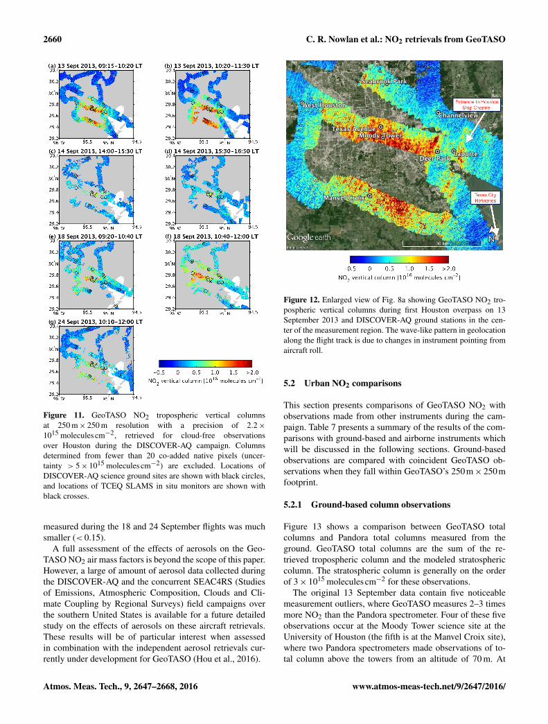
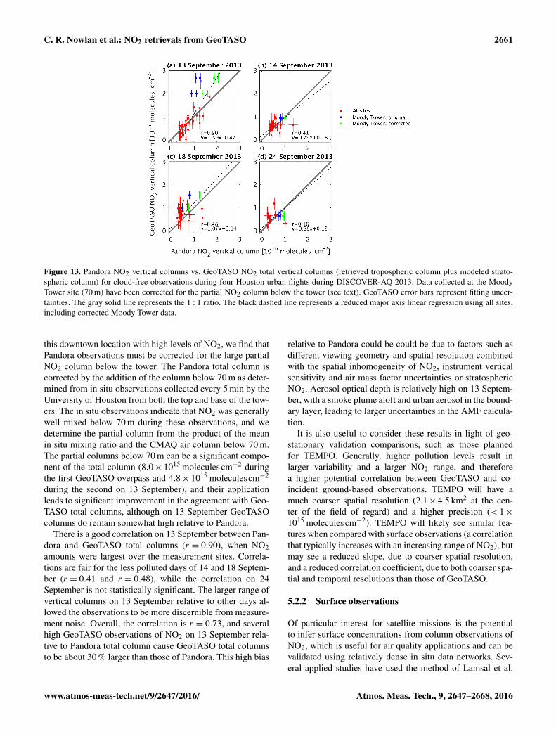
Figure 11 shows NO2 tropospheric vertical columns derivedfrom GeoTASO during 4 days of DISCOVER-AQ flightsover the Houston area. The 13 September was the day withthe highest levels of detected NO2 and also the day most freeof clouds. Figure 12 shows an enlarged view of the first over-pass of this day over urban Houston. In these 13 Septemberflights, the two most polluted overpasses occur over down-town Houston and several large freeways (I-10, I-45, I-69,I-610) and their interchanges. The more southern pollutedoverpass occurs over the more rural and suburban Route 6,and the Manvel Croix science site. Although there are fewlocal sources of pollution, the suburban Manvel region ofHouston regularly has some of the highest ozone concentra-tions in the Houston area (Sather and Cavender, 2012).
While the majority of NO2 appears correlated with roadsand highly populated areas, enhanced levels of NO2 are alsodetectable over industrial facilities, including those to theeast of Houston near the entrance of the Houston ship chan-nel, and the petrochemical manufacturing and petroleum re-fineries at Texas City near Galveston Bay.
Aerosol optical depths measured by the HSRL lidar on theNASA King Air at 532 nm and by an Aerosol Robotic Net-work (AERONET) instrument (http://aeronet.gsfc.nasa.gov/)at Moody Tower at 441 nm indicate that maximum aerosoloptical depths (AOD) were as large as 0.4 on 13 Septem-ber and 0.7 on 14 September. HSRL data indicate that asmoke plume present at 2–3 km on the 13th contributed tothe larger AOD on this day, and also show significant urbanpollution aerosols in the boundary layer. The smoke plumeremained on the 14th, but HSRL data indicate that urban pol-lution aerosols at lower altitudes were the main contributorto the AOD. At these AODs, NO2 AMF biases calculated byLin et al. (2014) are typically within ± 25 %. Aerosol AOD
2660 C. R. Nowlan et al.: NO2 retrievals from GeoTASO
Figure 11. GeoTASO NO2 tropospheric vertical columnsat 250 m× 250 m resolution with a precision of 2.2×10¹⁵ moleculescm−2, retrieved for cloud-free observationsover Houston during the DISCOVER-AQ campaign. Columnsdetermined from fewer than 20 co-added native pixels (uncer-tainty > 5× 10¹⁵ moleculescm−2) are excluded. Locations ofDISCOVER-AQ science ground sites are shown with black circles,and locations of TCEQ SLAMS in situ monitors are shown withblack crosses.
measured during the 18 and 24 September flights was muchsmaller (< 0.15).
A full assessment of the effects of aerosols on the Geo-TASO NO2 air mass factors is beyond the scope of this paper.However, a large of amount of aerosol data collected duringthe DISCOVER-AQ and the concurrent SEAC4RS (Studiesof Emissions, Atmospheric Composition, Clouds and Cli-mate Coupling by Regional Surveys) field campaigns overthe southern United States is available for a future detailedstudy on the effects of aerosols on these aircraft retrievals.These results will be of particular interest when assessedin combination with the independent aerosol retrievals cur-rently under development for GeoTASO (Hou et al., 2016).
Figure 12. Enlarged view of Fig. 8a showing GeoTASO NO2 tro-pospheric vertical columns during first Houston overpass on 13September 2013 and DISCOVER-AQ ground stations in the cen-ter of the measurement region. The wave-like pattern in geolocationalong the flight track is due to changes in instrument pointing fromaircraft roll.
5.2 Urban NO2 comparisons
This section presents comparisons of GeoTASO NO2 withobservations made from other instruments during the cam-paign. Table 7 presents a summary of the results of the com-parisons with ground-based and airborne instruments whichwill be discussed in the following sections. Ground-basedobservations are compared with coincident GeoTASO ob-servations when they fall within GeoTASO’s 250m× 250mfootprint.
5.2.1 Ground-based column observations
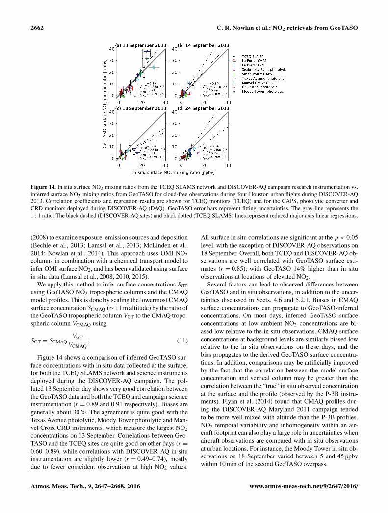
Figure 13 shows a comparison between GeoTASO totalcolumns and Pandora total columns measured from theground. GeoTASO total columns are the sum of the re-trieved tropospheric column and the modeled stratosphericcolumn. The stratospheric column is generally on the orderof 3× 10¹⁵ moleculescm−2 for these observations.
The original 13 September data contain five noticeablemeasurement outliers, where GeoTASO measures 2–3 timesmore NO2 than the Pandora spectrometer. Four of these fiveobservations occur at the Moody Tower science site at theUniversity of Houston (the fifth is at the Manvel Croix site),where two Pandora spectrometers made observations of to-tal column above the towers from an altitude of 70 m. At
C. R. Nowlan et al.: NO2 retrievals from GeoTASO 2661
Figure 13. Pandora NO2 vertical columns vs. GeoTASO NO2 total vertical columns (retrieved tropospheric column plus modeled strato-spheric column) for cloud-free observations during four Houston urban flights during DISCOVER-AQ 2013. Data collected at the MoodyTower site (70 m) have been corrected for the partial NO2 column below the tower (see text). GeoTASO error bars represent fitting uncer-tainties. The gray solid line represents the 1 : 1 ratio. The black dashed line represents a reduced major axis linear regression using all sites,including corrected Moody Tower data.
this downtown location with high levels of NO2, we find thatPandora observations must be corrected for the large partialNO2 column below the tower. The Pandora total column iscorrected by the addition of the column below 70 m as deter-mined from in situ observations collected every 5 min by theUniversity of Houston from both the top and base of the tow-ers. The in situ observations indicate that NO2 was generallywell mixed below 70 m during these observations, and wedetermine the partial column from the product of the meanin situ mixing ratio and the CMAQ air column below 70 m.The partial columns below 70 m can be a significant compo-nent of the total column (8.0× 10¹⁵ moleculescm−2 duringthe first GeoTASO overpass and 4.8× 10¹⁵ moleculescm−2
during the second on 13 September), and their applicationleads to significant improvement in the agreement with Geo-TASO total columns, although on 13 September GeoTASOcolumns do remain somewhat high relative to Pandora.
There is a good correlation on 13 September between Pan-dora and GeoTASO total columns (r = 0.90), when NO2amounts were largest over the measurement sites. Correla-tions are fair for the less polluted days of 14 and 18 Septem-ber (r = 0.41 and r = 0.48), while the correlation on 24September is not statistically significant. The larger range ofvertical columns on 13 September relative to other days al-lowed the observations to be more discernible from measure-ment noise. Overall, the correlation is r = 0.73, and severalhigh GeoTASO observations of NO2 on 13 September rela-tive to Pandora total column cause GeoTASO total columnsto be about 30 % larger than those of Pandora. This high bias
relative to Pandora could be could be due to factors such asdifferent viewing geometry and spatial resolution combinedwith the spatial inhomogeneity of NO2, instrument verticalsensitivity and air mass factor uncertainties or stratosphericNO2. Aerosol optical depth is relatively high on 13 Septem-ber, with a smoke plume aloft and urban aerosol in the bound-ary layer, leading to larger uncertainties in the AMF calcula-tion.
It is also useful to consider these results in light of geo-stationary validation comparisons, such as those plannedfor TEMPO. Generally, higher pollution levels result inlarger variability and a larger NO2 range, and thereforea higher potential correlation between GeoTASO and co-incident ground-based observations. TEMPO will have amuch coarser spatial resolution (2.1× 4.5 km2 at the cen-ter of the field of regard) and a higher precision (< 1×10¹⁵ moleculescm−2). TEMPO will likely see similar fea-tures when compared with surface observations (a correlationthat typically increases with an increasing range of NO2), butmay see a reduced slope, due to coarser spatial resolution,and a reduced correlation coefficient, due to both coarser spa-tial and temporal resolutions than those of GeoTASO.
5.2.2 Surface observations
Of particular interest for satellite missions is the potentialto infer surface concentrations from column observations ofNO2, which is useful for air quality applications and can bevalidated using relatively dense in situ data networks. Sev-eral applied studies have used the method of Lamsal et al.
2662 C. R. Nowlan et al.: NO2 retrievals from GeoTASO
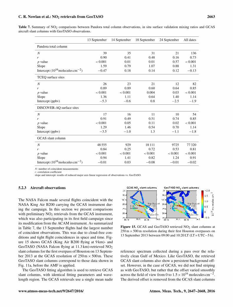
Figure 14. In situ surface NO2 mixing ratios from the TCEQ SLAMS network and DISCOVER-AQ campaign research instrumentation vs.inferred surface NO2 mixing ratios from GeoTASO for cloud-free observations during four Houston urban flights during DISCOVER-AQ2013. Correlation coefficients and regression results are shown for TCEQ monitors (TCEQ) and for the CAPS, photolytic converter andCRD monitors deployed during DISCOVER-AQ (DAQ). GeoTASO error bars represent fitting uncertainties. The gray line represents the1 : 1 ratio. The black dashed (DISCOVER-AQ sites) and black dotted (TCEQ SLAMS) lines represent reduced major axis linear regressions.
(2008) to examine exposure, emission sources and deposition(Bechle et al., 2013; Lamsal et al., 2013; McLinden et al.,2014; Nowlan et al., 2014). This approach uses OMI NO2columns in combination with a chemical transport model toinfer OMI surface NO2, and has been validated using surfacein situ data (Lamsal et al., 2008, 2010, 2015).
We apply this method to infer surface concentrations SGTusing GeoTASO NO2 tropospheric columns and the CMAQmodel profiles. This is done by scaling the lowermost CMAQsurface concentration SCMAQ (∼ 11 m altitude) by the ratio ofthe GeoTASO tropospheric column VGT to the CMAQ tropo-spheric column VCMAQ using
SGT = SCMAQVGT
VCMAQ. (11)
Figure 14 shows a comparison of inferred GeoTASO sur-face concentrations with in situ data collected at the surface,for both the TCEQ SLAMS network and science instrumentsdeployed during the DISCOVER-AQ campaign. The pol-luted 13 September day shows very good correlation betweenthe GeoTASO data and both the TCEQ and campaign scienceinstrumentation (r = 0.89 and 0.91 respectively). Biases aregenerally about 30 %. The agreement is quite good with theTexas Avenue photolytic, Moody Tower photolytic and Man-vel Croix CRD instruments, which measure the largest NO2concentrations on 13 September. Correlations between Geo-TASO and the TCEQ sites are quite good on other days (r =0.60–0.89), while correlations with DISCOVER-AQ in situinstrumentation are slightly lower (r = 0.49–0.74), mostlydue to fewer coincident observations at high NO2 values.
All surface in situ correlations are significant at the p < 0.05level, with the exception of DISCOVER-AQ observations on18 September. Overall, both TCEQ and DISCOVER-AQ ob-servations are well correlated with GeoTASO surface esti-mates (r = 0.85), with GeoTASO 14% higher than in situobservations at locations of elevated NO2.
Several factors can lead to observed differences betweenGeoTASO and in situ observations, in addition to the uncer-tainties discussed in Sects. 4.6 and 5.2.1. Biases in CMAQsurface concentrations can propagate to GeoTASO-inferredconcentrations. On most days, inferred GeoTASO surfaceconcentrations at low ambient NO2 concentrations are bi-ased low relative to the in situ observations. CMAQ surfaceconcentrations at background levels are similarly biased lowrelative to the in situ observations on these days, and thebias propagates to the derived GeoTASO surface concentra-tions. In addition, comparisons may be artificially improvedby the fact that the correlation between the model surfaceconcentration and vertical column may be greater than thecorrelation between the “true” in situ observed concentrationat the surface and the profile (observed by the P-3B instru-ments). Flynn et al. (2014) found that CMAQ profiles dur-ing the DISCOVER-AQ Maryland 2011 campaign tendedto be more well mixed with altitude than the P-3B profiles.NO2 temporal variability and inhomogeneity within an air-craft footprint can also play a large role in uncertainties whenaircraft observations are compared with in situ observationsat urban locations. For instance, the Moody Tower in situ ob-servations on 18 September varied between 5 and 45 ppbvwithin 10 min of the second GeoTASO overpass.
C. R. Nowlan et al.: NO2 retrievals from GeoTASO 2663
Table 7. Summary of NO2 comparisons between Pandora total column observations, in situ surface validation mixing ratios and GCASaircraft slant columns with GeoTASO observations.
13 September 14 September 18 September 24 September All dates
N : number of coincident measurementsr: correlation coefficientslope and intercept: results of reduced major axis linear regression of observations vs. GeoTASO.
5.2.3 Aircraft observations
The NASA Falcon made several flights coincident with theNASA King Air B200 carrying the GCAS instrument dur-ing the campaign. In this section we present comparisonswith preliminary NO2 retrievals from the GCAS instrument,which was also participating in its first field campaign sinceits modification from the ACAM instrument. As summarizedin Table 7, the 13 September flights had the largest numberof coincident observations. This was due to cloud-free con-ditions and tight flight coincidences in space and time. Fig-ure 15 shows GCAS (King Air B200 flying at 9 km)- andGeoTASO (NASA Falcon flying at 11.3 km)-retrieved NO2slant columns for the first overpass of Houston on 13 Septem-ber 2013 at the GCAS resolution of 250m× 500m. TheseGeoTASO slant columns correspond to those data shown inFig. 11a, before the AMF is applied.
The GeoTASO fitting algorithm is used to retrieve GCASslant columns, with identical fitting parameters and wave-length region. The GCAS retrievals use a single mean nadir
Figure 15. GCAS and GeoTASO retrieved NO2 slant columns at250 m× 500 m resolution during their first Houston overpasses on13 September 2013 between 09:00 and 10:20 LT (LT = UTC−5 h).
reference spectrum collected during a pass over the rela-tively clean Gulf of Mexico. Like GeoTASO, the retrievedGCAS slant columns also show a persistent background off-set. However, in the case of GCAS, we did not find stripingas with GeoTASO, but rather that the offset varied smoothlyacross the field of view from 0 to 1.5×10¹⁶ moleculescm−2.The derived offset is removed from the GCAS slant columns
2664 C. R. Nowlan et al.: NO2 retrievals from GeoTASO
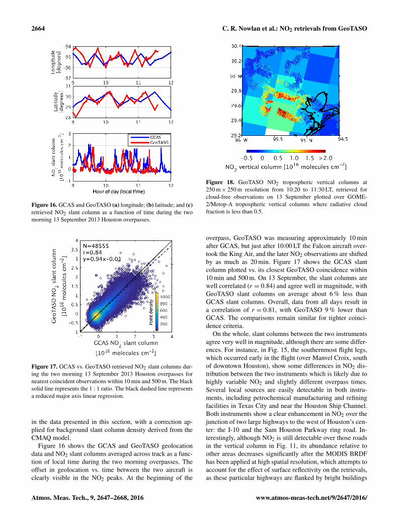
Figure 16. GCAS and GeoTASO (a) longitude; (b) latitude; and (c)retrieved NO2 slant column as a function of time during the twomorning 13 September 2013 Houston overpasses.
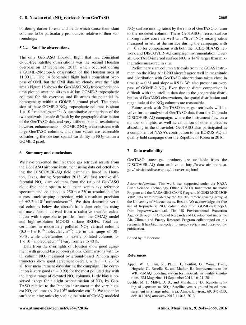
Figure 17. GCAS vs. GeoTASO retrieved NO2 slant columns dur-ing the two morning 13 September 2013 Houston overpasses fornearest coincident observations within 10 min and 500 m. The blacksolid line represents the 1 : 1 ratio. The black dashed line representsa reduced major axis linear regression.
in the data presented in this section, with a correction ap-plied for background slant column density derived from theCMAQ model.
Figure 16 shows the GCAS and GeoTASO geolocationdata and NO2 slant columns averaged across track as a func-tion of local time during the two morning overpasses. Theoffset in geolocation vs. time between the two aircraft isclearly visible in the NO2 peaks. At the beginning of the
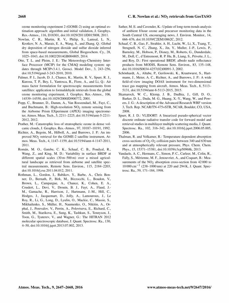
Figure 18. GeoTASO NO2 tropospheric vertical columns at250 m× 250 m resolution from 10:20 to 11:30 LT, retrieved forcloud-free observations on 13 September plotted over GOME-2/Metop-A tropospheric vertical columns where radiative cloudfraction is less than 0.5.
overpass, GeoTASO was measuring approximately 10 minafter GCAS, but just after 10:00 LT the Falcon aircraft over-took the King Air, and the later NO2 observations are shiftedby as much as 20 min. Figure 17 shows the GCAS slantcolumn plotted vs. its closest GeoTASO coincidence within10 min and 500 m. On 13 September, the slant columns arewell correlated (r = 0.84) and agree well in magnitude, withGeoTASO slant columns on average about 6 % less thanGCAS slant columns. Overall, data from all days result ina correlation of r = 0.81, with GeoTASO 9 % lower thanGCAS. The comparisons remain similar for tighter coinci-dence criteria.
On the whole, slant columns between the two instrumentsagree very well in magnitude, although there are some differ-ences. For instance, in Fig. 15, the southernmost flight legs,which occurred early in the flight (over Manvel Croix, southof downtown Houston), show some differences in NO2 dis-tribution between the two instruments which is likely due tohighly variable NO2 and slightly different overpass times.Several local sources are easily detectable in both instru-ments, including petrochemical manufacturing and refiningfacilities in Texas City and near the Houston Ship Channel.Both instruments show a clear enhancement in NO2 over thejunction of two large highways to the west of Houston’s cen-ter: the I-10 and the Sam Houston Parkway ring road. In-terestingly, although NO2 is still detectable over those roadsin the vertical column in Fig. 11, its abundance relative toother areas decreases significantly after the MODIS BRDFhas been applied at high spatial resolution, which attempts toaccount for the effect of surface reflectivity on the retrievals,as these particular highways are flanked by bright buildings
C. R. Nowlan et al.: NO2 retrievals from GeoTASO 2665
bordering darker forests and fields which cause their slantcolumns to be particularly pronounced relative to their sur-roundings.
5.2.4 Satellite observations
The only GeoTASO Houston flight that had coincidentcloud-free satellite observations was the second Houstonoverpass on 13 September 2013, which occurred duringa GOME-2/Metop-A observation of the Houston area at11:00 LT. (The 14 September flight had a coincident over-pass of OMI, but the OMI data are cloudy over the flightarea.) Figure 18 shows the GeoTASO NO2 tropospheric col-umn plotted over the 40km× 40km GOME-2 troposphericcolumns for this overpass, and illustrates the potential in-homogeneity within a GOME-2 ground pixel. The preci-sion of these GOME-2 NO2 tropospheric columns is about1× 1015 molecules cm−2. A quantitative comparison of thetwo retrievals is made difficult by the geographic distributionof the GeoTASO data and very different spatial resolutions;however, enhancements in GOME-2 NO2 are consistent withlarge GeoTASO columns, and mean values are reasonableconsidering the obvious spatial variability in NO2 within aGOME-2 pixel.
6 Summary and conclusions
We have presented the first trace gas retrieval results fromthe GeoTASO airborne instrument using data collected dur-ing the DISCOVER-AQ field campaign based in Hous-ton, Texas, during September 2013. We first retrieve dif-ferential NO2 slant columns from the ratio of GeoTASOcloud-free nadir spectra to a mean zenith sky referencespectrum and co-added to 250m× 250m resolution aftera cross-track striping correction, with a resultant precisionof ±2.2× 10¹⁵ moleculescm−2. We then determine verti-cal columns below the aircraft from slant columns usingair mass factors derived from a radiative transfer calcu-lation with tropospheric profiles from the CMAQ modeland high-resolution MODIS surface BRDFs. Total un-certainties in moderately polluted NO2 vertical columns(0.3− 1× 10¹⁶ moleculescm−2) are in the range of 30–80 %, while uncertainties in heavily polluted columns (>1× 10¹⁶ molecules cm−2) vary from 27 to 40 %.
Data from the overflights of Houston show good agree-ment with ground-based observations. Comparisons with to-tal column NO2 measured by ground-based Pandora spec-trometers show good agreement overall, with r = 0.73 forall four measurement days during the campaign. The corre-lation is very good (r = 0.90) for the most polluted day withthe largest range of elevated NO2 columns. Little bias is ob-served except for a slight overestimation of NO2 by Geo-TASO relative to the Pandora instrument at the very high-est NO2 columns (> 2×10¹⁶ moleculescm−2). We also infersurface mixing ratios by scaling the ratio of CMAQ-modeled
NO2 surface mixing ratios by the ratio of GeoTASO columnto the modeled column. These GeoTASO-inferred surfacemixing ratios correlate well with “true” NO2 mixing ratiosmeasured in situ at the surface during the campaign, withr = 0.85 for comparisons with both the TCEQ SLAMS net-work and DISCOVER-AQ campaign instrumentation. Over-all, GeoTASO-inferred surface NO2 is 14 % larger than mix-ing ratios measured in situ.
Preliminary slant column retrievals from the GCAS instru-ment on the King Air B200 aircraft agree well in magnitudeand distribution with GeoTASO observations taken close intime (r = 0.81 and slope= 0.91). We also present an over-pass of GOME-2 NO2. Even though direct comparison isdifficult with the satellite data due to the geographic distri-bution of GeoTASO observations, the spatial distribution andmagnitude of the NO2 columns are reasonable.
Future work with GeoTASO trace gas retrievals will in-volve further analysis of GeoTASO data from the ColoradoDISCOVER-AQ campaign, where the instrument flew on anumber of flights, as well as validation of other moleculesabsorbing in the ultraviolet. GeoTASO also participated asa component of NASA’s contribution to the KORUS-AQ airquality field campaign over the Republic of Korea in 2016.
7 Data availability
GeoTASO trace gas products are available from theDISCOVER-AQ data archive at http://www-air.larc.nasa.gov/missions/discover-aq/discover-aq.html.
Acknowledgements. This work was supported under the NASAEarth Science Technology Office (ESTO) Instrument IncubatorProgram and the NASA GEO-CAPE Program. MODIS MCD43GFV005 data were provided by the MODIS remote sensing group atthe University of Massachusetts, Boston. We acknowledge the freeuse of tropospheric NO2 column data from GOME-2/Metop-Afrom http://www.temis.nl. The US Environmental ProtectionAgency through its Office of Research and Development under theAir, Climate and Energy Research Program collaborated on thisresearch. It has been subjected to agency review and approved forpublication.
Edited by: F. Boersma
References
Appel, W., Gilliam, R., Pleim, J., Pouliot, G., Wong, D.-C.,Hogrefe, C., Roselle, S., and Mathur, R.: Improvements to theWRF-CMAQ modeling system for fine-scale air quality simula-tions, EM Magazine, 14 September 2014, 16–21, 2014.
Bechle, M. J., Millet, D. B., and Marshall, J. D.: Remote sens-ing of exposure to NO2: Satellite versus ground-based mea-surement in a large urban area, Atmos. Environ., 69, 345–353,doi:10.1016/j.atmosenv.2012.11.046, 2013.
2666 C. R. Nowlan et al.: NO2 retrievals from GeoTASO
Boersma, K. F., Eskes, H. J., and Brinksma, E. J.: Error analysis fortropospheric NO2 retrieval from space, J. Geophys. Res.-Atmos.,109, D04311, doi:10.1029/2003JD003962, 2004.
Boersma, K. F., Eskes, H. J., Dirksen, R. J., van der A, R. J.,Veefkind, J. P., Stammes, P., Huijnen, V., Kleipool, Q. L., Sneep,M., Claas, J., Leitão, J., Richter, A., Zhou, Y., and Brunner, D.:An improved tropospheric NO2 column retrieval algorithm forthe Ozone Monitoring Instrument, Atmos. Meas. Tech., 4, 1905–1928, doi:10.5194/amt-4-1905-2011, 2011.
Bourassa, A. E., McLinden, C. A., Sioris, C. E., Brohede, S., Bath-gate, A. F., Llewellyn, E. J., and Degenstein, D. A.: Fast NO2retrievals from Odin-OSIRIS limb scatter measurements, Atmos.Meas. Tech., 4, 965–972, doi:10.5194/amt-4-965-2011, 2011.
Brent, L. C., Thorn, W. J., Gupta, M., Leen, B., Stehr, J. W., He,H., Arkinson, H. L., Weinheimer, A., Garland, C., Pusede, S. E.,Wooldridge, P. J., Cohen, R. C., and Dickerson, R. R.: Evaluationof the use of a commercially available cavity ringdown absorp-tion spectrometer for measuring NO2 in flight, and observationsover the Mid-Atlantic States, during DISCOVER-AQ, J. Atmos.Chem., 72, 1–19, doi:10.1007/s10874-013-9265-6, 2013.
Brinksma, E., de Haan, J., Boersma, F., Bucsela, E., and Glea-son, J. F.: Appendix A: Air mass factors over polluted scenes, in:OMI Algorithm Theoretical Basis Document, Volume IV: OMITrace Gas Algorithms, edited by: Chance, K., NASA GSFC,Greenbelt, MD, USA, 29–32, 2002.
Brion, J., Chakir, A., Daumont, D., Malicet, J., and Parisse, C.:High-resolution laboratory absorption cross section of O3, Tem-perature effect, Chem. Phys. Lett., 213, 610–612, 1993.
Bucsela, E. J., Krotkov, N. A., Celarier, E. A., Lamsal, L. N.,Swartz, W. H., Bhartia, P. K., Boersma, K. F., Veefkind, J. P.,Gleason, J. F., and Pickering, K. E.: A new stratospheric andtropospheric NO2 retrieval algorithm for nadir-viewing satelliteinstruments: applications to OMI, Atmos. Meas. Tech., 6, 2607–2626, doi:10.5194/amt-6-2607-2013, 2013.
Byun, D. and Schere, K. L.: Review of the governing equations,computational algorithms, and other components of the Models-3 Community Multiscale Air Quality (CMAQ) modeling system,Appl. Mech. Rev., 59, 51–77, doi:10.1115/1.2128636, 2006.
Cai, Z., Liu, Y., Liu, X., Chance, K., Nowlan, C. R., Lang, R.,Munro, R., and Suleiman, R.: Characterization and correctionof global ozone monitoring experiment 2 ultraviolet measure-ments and application to ozone profile retrievals, J. Geophys.Res.-Atmos., 117, D07305, doi:10.1029/2011JD017096, 2012.
Chan Miller, C., Gonzalez Abad, G., Wang, H., Liu, X., Kurosu,T., Jacob, D. J., and Chance, K.: Glyoxal retrieval from theOzone Monitoring Instrument, Atmos. Meas. Tech., 7, 3891–3907, doi:10.5194/amt-7-3891-2014, 2014.
Chance, K. and Kurucz, R. L.: An improved high-resolution solarreference spectrum for Earth’s atmosphere measurements in theultraviolet, visible, and near infrared, J. Quant. Spectrosc. Ra.,111, 1289–1295, doi:10.1016/j.jqsrt.2010.01.036, 2010.
Chance, K.: Analysis of BrO measurements from the Global OzoneMonitoring Experiment, Geophys. Res. Lett., 25, 3335–3338,1998.
Chance, K., Palmer, P. I., Spurr, R. J., Martin, R. V., Kurosu, T. P.,and Jacob, D. J.: Satellite observations of formaldehyde overNorth America from GOME, Geophys. Res. Lett., 27, 3461–3464, 2000.
Chance, K., Kurosu, T. P., and Sioris, C. E.: Undersampling correc-tion for array detector-based satellite spectrometers, Appl. Op-tics, 44, 1296–1304, doi:10.1364/AO.44.001296, 2005.
Chance, K., Liu, X., Suleiman, R. M., Flittner, D. E., Al-Saadi, J.,and Janz, S. J.: Tropospheric emissions: monitoring of pollution(TEMPO), Proc. SPIE 8866, Earth Observing Systems XVIII,8866, 88660D-1–88660D-16, doi:10.1117/12.2024479, 2013.
Chance, K. V. and Spurr, R. J. D.: Ring effect studies: Rayleighscattering, including molecular parameters for rotational Ramanscattering, and the Fraunhofer spectrum, Appl. Optics, 36, 5224–5230, 1997.
Fishman, J., Iraci, L. T., Al-Saadi, J., Chance, K., Chavez, F.,Chin, M., Coble, P., Davis, C., DiGiacomo, P. M., Edwards, D.,Eldering, A., Goes, J., Herman, J., Hu, C., Jacob, D. J., Jor-dan, C., Kawa, S. R., Key, R., Liu, X., Lohrenz, S., Man-nino, A., Natraj, V., Neil, D., Neu, J., Newchurch, M., Picker-ing, K., Salisbury, J., Sosik, H., Subramaniam, A., Tzortziou,M., Wang, J., and Wang, M.: The United States’ next gener-ation of atmospheric composition and coastal ecosystem mea-surements: NASA’s geostationary coastal and air pollution events(GEO-CAPE) mission, B. Am. Meteorol. Soc., 93, 1547–1566,doi:10.1175/bams-d-11-00201.1, 2012.
Flynn, C. M., Pickering, K. E., Crawford, J. H., Lamsal, L.,Krotkov, N., Herman, J., Weinheimer, A., Chen, G., Liu, X.,Szykman, J., Tsay, S.-C., Loughner, C., Hains, J., Lee, P.,Dickerson, R. R., Stehr, J. W., and Brent, L.: Relationshipbetween column-density and surface mixing ratio: Statisticalanalysis of O3 and NO2 data from the July 2011 Mary-land DISCOVER-AQ mission, Atmos. Environ., 92, 429–441,doi:10.1016/j.atmosenv.2014.04.041, 2014.
General, S., Pöhler, D., Sihler, H., Bobrowski, N., Frieß, U., Ziel-cke, J., Horbanski, M., Shepson, P. B., Stirm, B. H., Simpson,W. R., Weber, K., Fischer, C., and Platt, U.: The HeidelbergAirborne Imaging DOAS Instrument (HAIDI) – a novel imag-ing DOAS device for 2-D and 3-D imaging of trace gases andaerosols, Atmos. Meas. Tech., 7, 3459–3485, doi:10.5194/amt-7-3459-2014, 2014.
González Abad, G., Vasilkov, A., Seftor, C., Liu, X., and Chance,K.: Smithsonian Astrophysical Observatory Ozone Mapping andProfiler Suite (SAO OMPS) formaldehyde retrieval, Atmos.Meas. Tech. Discuss., 8, 9209–9240, doi:10.5194/amtd-8-9209-2015, 2015b.
Hair, J. W., Hostetler, C. A., Cook, A. L., Harper, D. B., Fer-rare, R. A., Mack, T. L., Welch, W., Izquierdo, L. R., andHovis, F. E.: Airborne high spectral resolution lidar for pro-filing aerosol optical properties, Appl. Optics, 47, 6734–6752,doi:10.1364/AO.47.006734, 2008.
Herman, J., Cede, A., Spinei, E., Mount, G., Tzortziou, M.,and Abuhassan, N.: NO2 column amounts from ground-based Pandora and MFDOAS spectrometers using the direct-sun DOAS technique: Intercomparisons and application toOMI validation, J. Geophys. Res.-Atmos., 114, D13307,doi:10.1029/2009JD011848, 2009.
C. R. Nowlan et al.: NO2 retrievals from GeoTASO 2667
Heue, K.-P., Wagner, T., Broccardo, S. P., Walter, D., Piketh, S.J., Ross, K. E., Beirle, S., and Platt, U.: Direct observation oftwo dimensional trace gas distributions with an airborne Imag-ing DOAS instrument, Atmos. Chem. Phys., 8, 6707–6717,doi:10.5194/acp-8-6707-2008, 2008.
Hou, W., Wang, J., Xu, X., Reid, J. S., and Han, D.: VLIDORT:An algorithm for hyperspectral remote sensing of aerosols: 1.Development of theoretical framework, J. Quant. Spectrosc. Ra.,178, 400–415, doi:10.1016/j.jqsrt.2016.01.019, 2016.
Illing, R. M. E.: Design and development of the PolZero TimeDomain Polarization Scrambler, Proc. SPIE, 7461, Polariza-tion Science and Remote Sensing IV, 746104-1–746104–10,doi:10.1117/12.826217, 2009.
Ingmann, P., Veihelmann, B., Langen, J., Lamarre, D., Stark, H.,and Courrèges-Lacoste, G. B.: Requirements for the GMESatmosphere service and ESA’s implementation concept:Sentinels-4/-5 and-5p, Remote Sens. Environ., 120, 58–69,doi:10.1016/j.rse.2012.01.023, 2012.
Kim, J.: GEMS (Geostationary Environment Monitoring Spectrom-eter) onboard the GeoKOMPSAT to Monitor Air Quality in highTemporal and Spatial Resolution over Asia-Pacific Region, in:EGU General Assembly Conference Abstracts, edited by: Ab-basi, A. and Giesen, N., Vol. 14, EGU General Assembly Con-ference Abstracts, 22–27 April 2012, Vienna, Austria, p. 4051,2012.
Kowalewski, M. G. and Janz, S. J.: Remote sensing capa-bilities of the GEO-CAPE airborne simulator, Proc. SPIE,9218, Earth Observing Systems XIX, 92181I–92181I–12,doi:10.1117/12.2062058, 2014.
Lamsal, L. N., Martin, R. V., Van Donkelaar, A., Steinbacher, M.,Celarier, E. A., Bucsela, E., Dunlea, E. J., and Pinto, J. P.:Ground-level nitrogen dioxide concentrations inferred from thesatellite-borne Ozone Monitoring Instrument, J. Geophys. Res.-Atmos., 113, D16308, doi:10.1029/2007JD009235, 2008.
Lamsal, L. N., Martin, R. V., Van Donkelaar, A., Celar-ier, E. A., Bucsela, E. J., Boersma, K. F., Dirksen, R.,Luo, C., and Wang, Y.: Indirect validation of tropospheric ni-trogen dioxide retrieved from the OMI satellite instrument:Insight into the seasonal variation of nitrogen oxides atnorthern midlatitudes, J. Geophys. Res.-Atmos., 115, D05302,doi:10.1029/2009JD013351, 2010.
Lamsal, L. N., Martin, R. V., Parrish, D. D., and Krotkov, N. A.:Scaling relationship for NO2 pollution and urban populationsize: a satellite perspective, Environ. Sci. Technol., 47, 7855–7861, doi:10.1021/es400744g, 2013.
Lamsal, L. N., Duncan, B. N., Yoshida, Y., Krotkov, N. A.,Pickering, K. E., Streets, D. G., and Lu, Z.: U. S.NO2 trends (2005–2013): EPA Air Quality System (AQS)data versus improved observations from the Ozone Mon-itoring Instrument (OMI), Atmos. Environ., 110, 130–143,doi:10.1016/j.atmosenv.2015.03.055, 2015.
Lawrence, J. P., Anand, J. S., Vande Hey, J. D., White, J., Leigh,R. R., Monks, P. S., and Leigh, R. J.: High-resolution measure-ments from the airborne Atmospheric Nitrogen Dioxide Imager(ANDI), Atmos. Meas. Tech., 8, 4735–4754, doi:10.5194/amt-8-4735-2015, 2015.
Leitão, J., Richter, A., Vrekoussis, M., Kokhanovsky, A., Zhang, Q.J., Beekmann, M., and Burrows, J. P.: On the improvement ofNO2 satellite retrievals – aerosol impact on the airmass factors,
Leitch, J. W., Delker, T., Good, W., Ruppert, L., Murcray, F.,Chance, K., Liu, X., Nowlan, C., Janz, S. J., Krotkov, N. A.,Pickering, K. E., Kowalewski, M., and Wang, J.: The GeoTASOairborne spectrometer project, Earth Observing Systems XIX,Proc. SPIE, 9218, 92181H–92181H–9, doi:10.1117/12.2063763,2014.
Lin, J.-T., Martin, R. V., Boersma, K. F., Sneep, M., Stammes, P.,Spurr, R., Wang, P., Van Roozendael, M., Clémer, K., and Irie,H.: Retrieving tropospheric nitrogen dioxide from the OzoneMonitoring Instrument: effects of aerosols, surface reflectanceanisotropy, and vertical profile of nitrogen dioxide, Atmos.Chem. Phys., 14, 1441–1461, doi:10.5194/acp-14-1441-2014,2014.
Liu, C., Liu, X., Kowalewski, M. G., Janz, S. J., González Abad, G.,Pickering, K. E., Chance, K., and Lamsal, L. N.: Characterizationand verification of ACAM slit functions for trace-gas retrievalsduring the 2011 DISCOVER-AQ flight campaign, Atmos. Meas.Tech., 8, 751–759, doi:10.5194/amt-8-751-2015, 2015.
Liu, X., Chance, K., Sioris, C. E., Spurr, R. J. D., Kurosu, T. P., Mar-tin, R. V., and Newchurch, M. J.: Ozone profile and troposphericozone retrievals from the global ozone monitoring experiment:algorithm description and validation, J. Geophys. Res.-Atmos.,110, D20307, doi:10.1029/2005JD006240, 2005.
Liu, X., Bhartia, P. K., Chance, K., Spurr, R. J. D., and Kurosu, T. P.:Ozone profile retrievals from the Ozone Monitoring Instrument,Atmos. Chem. Phys., 10, 2521–2537, doi:10.5194/acp-10-2521-2010, 2010.
Loughner, C. P., Allen, D. J., Pickering, K. E., Zhang, D.-L.,Shou, Y.-X., and Dickerson, R. R.: Impact of fair-weather cu-mulus clouds and the Chesapeake Bay breeze on pollutanttransport and transformation, Atmos. Environ., 45, 4060–4072,doi:10.1016/j.atmosenv.2011.04.003, 2011.
Martin, R. V., Chance, K., Jacob, D. J., Kurosu, T. P., Spurr, R. J.,Bucsela, E., Gleason, J. F., Palmer, P. I., Bey, I., Fiore, A. M.,Li, Q., Yantosca, R. M., and Koelemeijer, R. B. A.: An improvedretrieval of tropospheric nitrogen dioxide from GOME, J. Geo-phys. Res.-Atmos., 107, ACH-9, doi:10.1029/2001JD001027,2002.
McLinden, C. A., Olsen, S. C., Hannegan, B., Wild, O.,Prather, M. J., and Sundet, J.: Stratospheric ozone in 3-D models:A simple chemistry and the cross-tropopause flux, J. Geophys.Res.-Atmos., 105, 14653–14665, 2000.
McLinden, C. A., Fioletov, V., Boersma, K. F., Kharol, S. K.,Krotkov, N., Lamsal, L., Makar, P. A., Martin, R. V., Veefkind,J. P., and Yang, K.: Improved satellite retrievals of NO2and SO2 over the Canadian oil sands and comparisons withsurface measurements, Atmos. Chem. Phys., 14, 3637–3656,doi:10.5194/acp-14-3637-2014, 2014.
Munro, R., Lang, R., Klaes, D., Poli, G., Retscher, C., Lind-strot, R., Huckle, R., Lacan, A., Grzegorski, M., Holdak, A.,Kokhanovsky, A., Livschitz, J., and Eisinger, M.: The GOME-2 instrument on the Metop series of satellites: instrument de-sign, calibration, and level 1 data processing – an overview, At-mos. Meas. Tech., 9, 1279–1301, doi:10.5194/amt-9-1279-2016,2016.
Nowlan, C. R., Liu, X., Chance, K., Cai, Z., Kurosu, T. P., Lee, C.,and Martin, R. V.: Retrievals of sulfur dioxide from the global
2668 C. R. Nowlan et al.: NO2 retrievals from GeoTASO
ozone monitoring experiment 2 (GOME-2) using an optimal es-timation approach: algorithm and initial validation, J. Geophys.Res.-Atmos., 116, D18301, doi:10.1029/2011JD015808, 2011.
Nowlan, C. R., Martin, R. V., Philip, S., Lamsal, L. N.,Krotkov, N. A., Marais, E. A., Wang, S., and Zhang, Q.: Globaldry deposition of nitrogen dioxide and sulfur dioxide inferredfrom space-based measurements, Global Biogeochem. Cy., 28,1025–1043, doi:10.1002/2014GB004805, 2014.
Otte, T. L. and Pleim, J. E.: The Meteorology-Chemistry Inter-face Processor (MCIP) for the CMAQ modeling system: up-dates through MCIPv3.4.1, Geosci. Model Dev., 3, 243–256,doi:10.5194/gmd-3-243-2010, 2010.
Palmer, P. I., Jacob, D. J., Chance, K., Martin, R. V., Spurr, R. J.,Kurosu, T. P., Bey, I., Yantosca, R., Fiore, A., and Li, Q.: Airmass factor formulation for spectroscopic measurements fromsatellites: application to formaldehyde retrievals from the globalozone monitoring experiment, J. Geophys. Res.-Atmos., 106,14539–14550, doi:10.1029/2000JD900772, 2001.
Popp, C., Brunner, D., Damm, A., Van Roozendael, M., Fayt, C.,and Buchmann, B.: High-resolution NO2 remote sensing fromthe Airborne Prism EXperiment (APEX) imaging spectrome-ter, Atmos. Meas. Tech., 5, 2211–2225, doi:10.5194/amt-5-2211-2012, 2012.
Prather, M.: Catastrophic loss of stratospheric ozone in dense vol-canic clouds, J. Geophys. Res.-Atmos., 97, 10187–10191, 1992.
Richter, A., Begoin, M., Hilboll, A., and Burrows, J. P.: An im-proved NO2 retrieval for the GOME-2 satellite instrument, At-mos. Meas. Tech., 4, 1147–1159, doi:10.5194/amt-4-1147-2011,2011.
Román, M. O., Gatebe, C. K., Schaaf, C. B., Poudyal, R.,Wang, Z., and King, M. D.: Variability in surface BRDF atdifferent spatial scales (30 m–500 m) over a mixed agricul-tural landscape as retrieved from airborne and satellite spec-tral measurements, Remote Sens. Environ., 115, 2184–2203,doi:10.1016/j.rse.2011.04.012, 2011.
Rothman, L., Gordon, I., Babikov, Y., Barbe, A., Chris Ben-ner, D., Bernath, P., Birk, M., Bizzocchi, L., Boudon, V.,Brown, L., Campargue, A., Chance, K., Cohen, E. A.,Coudert, L., Devi, V., Drouin, B. J., Fayt, A., Flaud, J.-M., Gamache, R., Harrison, J., Hartmann, J.-M., Hill, C.,Hodges, J., Jacquemart, D., Jolly, A., Lamouroux, J., LeRoy, R., Li, G., Long, D., Lyulin, O., Mackie, C., Massie, S.,Mikhailenko, S., Müller, H., Naumenko, O., Nikitin, A., Or-phal, J., Perevalov, V., Perrin, A., Polovtseva, E., Richard, C.,Smith, M., Starikova, E., Sung, K., Tashkun, S., Tennyson, J.,Toon, G., Tyuterev, V., and Wagner, G.: The HITRAN 2012molecular spectroscopic database, J. Quant. Spectrosc. Ra., 130,4–50, doi:10.1016/j.jqsrt.2013.07.002, 2013.
Sather, M. E. and Cavender, K.: Update of long-term trends analysisof ambient 8 hour ozone and precursor monitoring data in theSouth Central US, encouraging news, J. Environ. Monitor., 14,666–676, doi:10.1039/C2EM10862C, 2012.
Schaaf, C. B., Gao, F., Strahler, A. H., Lucht, W., Li, X., Tsang, T.,Strugnell, N. C., Zhang, X., Jin, Y., Muller, J.-P., Lewis, P.,Barnsley, M., Hobson, P., Disney, M., Roberts, G., Dunderdale,M., Doll, C., d’Entremont, R. P. Hu, B., Liang, S., Privette, J. L.,and Roy, D.: First operational BRDF, albedo nadir reflectanceproducts from MODIS, Remote Sens. Environ., 83, 135–148,doi:10.1016/S0034-4257(02)00091-3, 2002.
Schönhardt, A., Altube, P., Gerilowski, K., Krautwurst, S., Hart-mann, J., Meier, A. C., Richter, A., and Burrows, J. P.: A widefield-of-view imaging DOAS instrument for two-dimensionaltrace gas mapping from aircraft, Atmos. Meas. Tech., 8, 5113–5131, doi:10.5194/amt-8-5113-2015, 2015.
Skamarock, W. C., Klemp, J. B., Dudhia, J., Gill, D. O.,Barker, D. L., Duda, M. G., Huang, X.-Y., Wang, W., and Pow-ers, J. G.: A description of the Advanced Research WRF version3, Tech. Rep. NCAR/TN-475+STR, NCAR, Boulder, CO, USA,2008.
Spurr, R. J. D.: VLIDORT: A linearized pseudo-spherical vectordiscrete ordinate radiative transfer code for forward model andretrieval studies in multilayer multiple scattering media, J. Quant.Spectrosc. Ra., 102, 316–342, doi:10.1016/j.jqsrt.2006.05.005,2006.
Thalman, R. and Volkamer, R.: Temperature dependent absorptioncross-sections of O2-O2 collision pairs between 340 and 630 nmand at atmospherically relevant pressure, Phys. Chem. Chem.Phys., 15, 15371–15381, doi:10.1039/c3cp50968k, 2013.
Vandaele, A. C., Hermans, C., Simon, P. C., Carleer, M., Colin, R.,Fally, S., Mérienne, M. F., Jenouvrier, A., and Coquart, B.: Mea-surements of the NO2 absorption cross-section from 42 000 to10 000 cm−1 (238–1000 nm) at 220 and 294 K, J. Quant. Spec-trosc. Ra., 59, 171–184, 1998.