NOAA Technical Memorandum ERL PMEL·103

TSUNAMI INUNDATION MODEL STUDY OF EUREKA AND CRESCENT CITY, CALIFORNIA

E. Bernard C. Mader G. Curtis K. Satake

Pacific Marine Environmental Laboratory Seattle, Washington November 1994

NATIONAL OCEANIC AND / Environmental Research ATMOSPHERIC ADMINISTRATION Laboratoriesn0 aa

NOAA Technical Memorandum ERL PMEL-103

TSUNAMI INUNDATION MODEL STUDY OF EUREKA AND CRESCENT CITY, CALIFORNIA

E. Bernard Pacific Marine Environmental Laboratory

C. Mader G. Curtis . JointJInstitute for Marine and Atmospheric Research University of Hawaii Honolulu, Hawaii

K. Satake University ofMichigan .Department of Geological Sciences Ann Arbor,Michigan

Pacific Marine Environmental Laboratory Seattle, Washington November 1994

UNITED STATES NATIONAL OCEANIC AND Environmental Research DEPARTMENT OF COMMERCE ATMOSPHERIC ADMINISTRATION Laboratories

Ronald H. Brown D. JAMES BAKER James L. Rasmussen DirectorSecretary Under Secrelary for Oceans

and Atmosphere/Administrator

, .

NOTICE

Mention of a commercial company or product does not constitute an endorsement by NOAAlERL. Use of information from this publication concerning proprietary products or the· tests of such products for publicity or advertising purposes is not authorized.

CAUTIONARY NOTE

The results of this study are intended for emergency planning purposes. Appropriate use would include the identification of evacuation zones. This study should WI be used for flood insurance purposes, because it is not based on a frequency analysis.

Contribution No. 1536 from NOAAlPacific Marine Environmental Laboratory

For sale by the National Technical Information Service, 5285 Port Royal Road Springfield, VA 22161

ii

CONTENTS PAGE

I ..INTRODUCTION· 1

2. TECHNICAL BACKGROUND ; 2

3. VALIDATION OF TSUNAMI MODELS 3

4. SCENARIOS OF POSSIBLE TSUNAMIS 4

5. TSUNAMI HAZARD IMPLICATIONS 6

6. CAUTIONARY NOTE ; 7

7. ACKNOWLEDGMENTS 7

8. REFERENCES ~ 7

Appendix A: Model Regional Descriptions (K. Satake) ; 9

Appendix B: Inundation Model Description (C.L. Mader) 15

Appendix C: The JIMAR Tsunami Research Effort Engineering Model for Tsunami Inundation (G.D. Curtis) 21

Appendix D: Regional Model Verification (K. Satake) 23

Appendix E: Modeling of the April 1992 Eureka Tsunami (C.L. Mader) 29

Appendix F: Verification of Crescent City Inundation Model 35

Appendix G: Earthquake Scenario Study with Regional Tsunami Model (K. Satake) 43­

Appendix H: Tsunami Inundation (C.L. Mader and G. Curtis) 67

Appendix I: Casca,dia Subduction Zone Earthquake Scenario Meeting ; 75

iii

Tsunami Inundation Model Study of Eureka and . Crescent City, California

E.N. BernardI, C. Made~, G. Curtis2, and K. Satake3

1. INTRODUCTION On April 25, 1992, a series of strong earthquakes occurred near Cape Mendocino, California.

The sequence began with an M -7.1 tremor at 11:06 a.m. (local time) on April 25. Strong aftershocks s

with 6.6 and 6.7 magnitudes occurred on April 26 at 00:41 a.m. and 4:18 a.m., respectively. These

three earthquakes and more than 2,000 recorded aftershocks illuminated the configuration of the

Mendocino Triple Junction, where the Pacific, North America, and southerninost Gorda plates meet.

The Ms-7.1 earthquake generated a small tsunami that was recorded by tide gauges from Oregon to

southern California. After detailed study of this earthquake, Oppenheimer et al. (1993) concluded

that

"The Cape Mendocino earthquake sequence provided seismological evidence that the

relative motion between the North America and Gorda plates results in significant thrust

earthquakes. In addition to the large ground motions generated by such shocks, they can

trigger equally hazardous aftershock sequences offshore in the Gorda plate and on the

Gorda-Pacific plate boundary. This sequence illustrates how a shallow thrust event, such as

the one of moment magnitude (M ) 8.5 that is forecast for the entire Cascadia subduction w

zone, could generate a tsunami of greater amplitude than the Cape Mendocino main shock.

Not only would this tsunami inundate communities along much of the Pacific Northwest

coast within minutes of the main shock, but it could persist for 8 hours at some locales."

On May 9, 1992, the Federal Emergency Management Agency (FEMA) hosted an after-action

discussion meeting with the scientificcommunity at the Presidio of San Francisco, California. From

these discussions, eight recommendations were formulated, including one to produce tsunami

inundation maps for northern California. The tsunami inundation study was ranked number two of

the eight and was identified as time-sensitive. NOAA responded to this recommendation by offering

to cost-share the study with FEMA and transmitted a proposal to FEMA on August 24, 1992. On

December 22, 1992, FEMA decided to fund the project, and funds were delivered to NOAA on

Pacific Marine Environmental Laboratory, National Oceanic and Atmospheric Administration, 7600 Sand Point Way NE, Seattle, WA 98115-0070.

2 Joint Institute for Marine and Atmospheric Research, University of Hawaii, 1000 Pope Road, Honolulu, HI 96822. .3 Department of Geological Sciences, University of Michigan, Ann Arbor, MI 48109-1063.

I

May 5, 1993. The project was completed on May 4, 1994, with this report representing a summary

of the study.

FEMA also funded the California Office of Emergency Services to examine other effects of a

larger Cascadia Subduction Zone earthquake-such as' ground shaking, liquefaction, and landslides.

A report entitled "Planning Scenario in Humboldt and Del Norte Counties for a Great Earthquake

on the Cascadia Subduction Zone" by Toppozada et al. includes hazards maps for emergency

planning purposes. This tsunami study was coordinated with the earthquake study through

discussions and meetings between Eddie Bernard and Tousson Toppozada of the California Division

of Mines and Geology. The tsunami effects described in the Toppozada et al. report were based on

the tsunami inundation maps described in this report.

The summary report consists of a project overview with appendixes to document the

scientific/technical details of each phase of the project. This format was chosen to provide an

overview for the nonspecialist while supplying scientific/technical details for the specialist. In this

way, we hope to reach a wide audience of readers interested in the tsunami hazard and illustrate the

use of some technical tools for emergency preparedness. E.N. Bernard (NOAA) prepared the

summary report while C.L. Mader (University of Hawaii) wrote the technical appendixes on

inundation modeling and K. Satake (University of Michigan) authored the technical appendixes on

earthquakes and regional modeling. George Curtis (University of Hawaii) wrote the appendix on an

engineering model.

2. TECHNICAL BACKGROUND The propagation of a tsunami from its source to a coastal area and the resultant flooding can be

mathematically depicted with reasonable accuracy by sets of coupled, partial-differential equations.

Analytical solutions of these equations are usually unattainable except in certain simplified cases.

However, solutions can be closely approximated, even in very difficult cases, by means of a number

of techniques well suited to use by computers. These solution schemes, referred to as numerical

models, can provide great insight into the nature of the process under study. Two such numerical

models, one a regional propagation model and the other an inundation model, have been applied to

the problem of examining the impact that a large, locally generated tsunami could have on

California. The models are described in detail in Appendixes. A and B. A third model, developed by

George Curtis (University of Hawaii), termed an engineering model, is presented in Appendix C.

The engineering model was used as an independent check on the Mader inundation model.

Redundancy such as the engineering model is desirable in studies for emergency preparedness.

Although the details of these models are described in Appendixes A, B, and C, two major items of

information needed to implement the models should be understood.

In the first place, if a model is to describe realistically the evolution of a tsunami from its source

to its termination, it must be provided with an accurate rendition of the shape of both the seafloor

over which the wave travels and the shape of the ground it potentially floods. This is accomplished

2

by compiling the bottom depths and land elevations of the area of interest. (See Appendixes A and

B for details.) For mathematical reasons, the model cannot use a continuously varying depiction of

topography butmust deal with discrete depths and elevations that have been averaged over a certain,

finite area. In the case of the regional model, the topography is provided on a model grid made up

of grid squares measuring 1.6 kIn on a side. For the inundation models, Crescent City is represented

by a 25-m grid while Humboldt Bay is modeled using a 100-m grid.

Knowledge of the nature of the numerical grid used in the model is the key to understanding the

results. Any topographic data point in the model represents the average depth/elevation over the

appropriate grid box. Quantities calculated by the model likewise represent average quantities over

the same areas. A calculated wave elevation of, say, 3.1 m above sea level does not mean that the

water everywhere in the appropriate grid would be uniformly 3.1 m above sea level. Rather, it means

that the water depth on that particular grid block averages roughly 3.1 m. In the same sense, if

flooding is indicated by the model in a grid block that contains both high and low elevations, this

does not necessarily imply flooding at the highest elevations. The point is that simulation results

must not be taken too literally but should be interpreted with a measure of common sense.

The second type of information needed to conduct tsunami simulations concerns the nature of

the waves approaching the threatened area. For this study, the regional model is first used to

generate the tsunami at the source and propagate the tsunami to the input boundary of the inundation

model, which can then perform the flooding computations.

Tsunami generation in the regional model is not a trivial matter and involves the depiction of

seafloor deformation by a major thrust earthquake. Based on our present understanding of tsunami

generation, however, vertical seafloor deformation (both uplift and subsidence) defines the initial

amplitude of the tsunami. Several different models exist that can calculate deformation patterns

based on assumptions about the slip, depth, length, width, and dip angle of the earthquake fault

plane. The problem becomes one of making intelligent estimates of these. parameters. To assist in

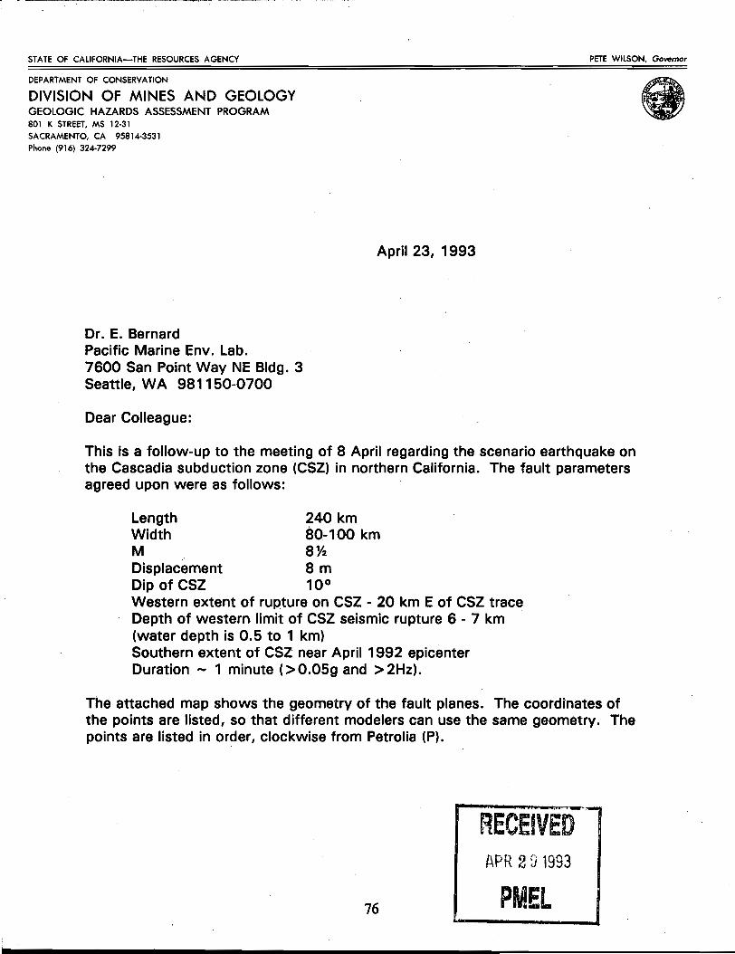
this process, Bernard and Satake attended a meeting of specialists to discuss the nature of

earthquakes in the Cascadia Subduction Zone on April 8, 1993, at the California Division of Mines

and Geology in Sacramento, California (see Appendix I); As a result of this meeting, four

earthquake scenarios were developed along with their corresponding fault-plane parameter sets

(Appendix I).

3. VALIDATION OF TSUNAMI MODELS The models used in this study have been tested extensively and have been applied toa variety

of cases publishe~ in the scientific literature (see Appendix A, B, and C). However, because ofthe

complexity of these models, it is always appropriate to compare simulations with observed data to

avoid errors. For this study, we used a combination of model results/data comparisons, and we used

independent computations with a third model for redundancy. Our principal data set was the 1992

3

Cape Mendocino earthquake/tsunami. The details of the comparison experiments are described in

Appendixes D and E. The regional model (1.6-km grid) used by Satake produced good agreement with eight tide

gauges that recorded this tsunami. He used the fault-plane parameters estimated by Oppenheimer

et at. (1993) to compute seafloor deformation and tsunami generation, and this produced a 30-cm

wave with period of about 30 min in an area offshore of Humboldt Bay (see Appendix D). As a

check, Mader used a l-km grid regional model with a slightly different generating mechanism and

obtained similar results offshore of Humboldt Bay (see Appendix E). The 30-cm wave with 30-min

period was then used as input for the inundation model. Good agreement was found between the tide

gauge record within Humboldt Bay at North Spit and the computed wave form (see Fig. E-3). We

were encouraged by these results since the model simulation produced both the amplitude and the

time sequence observed at the tide gauge. Inundation computations could not be checked because

this tsunami arrived at low tide and did not flood any areas. Furthermore, to our knowledge, no

tsunami inundation data exist for Humboldt Bay.

However, inundation data are available for the extensive flooding of Crescent City by the 1964

Alaska tsunami. These data were used to check an inundation model of Crescent City. The

numerical experiment is described in Mader and Bernard (1993), and the data/model comparison

is shown in Fig. 3 of that study (Appendix F).

In summary, the regional model was checked against the 1992 Cape Mendocino event and an

independent model run. The Humboldt Bay inundation model was checked against the 1992 tsunami

record at North Spit, and the Crescent City inundation model was checked against the 1964 Alaska

tsunami flooding survey.

4. SCENARIOS OF POSSIBLE TSUNAMIS We originally envisioned a straightforward approach to the development of earthquake

fault-plane estimates that would be used in regional models to provide tsunami input for the

inundation models. This worked well for the simulation of the 1992 Cape Mendocino earthquake

and was accepted practice in August 1992 (whenthe proposal for this study was submitted). We met

with specialists on the Cascadia Subduction Zone to define the type of earthquake that might be

expected from this area. These specialists are part of a different FEMA study to examine other

earthquake effects in this region such as ground shaking, liquefaction, and landslides. The results

of a I-day meeting on possible earthquake scenarios from the Cascadia Subduction Zone are

described in Appendix I where the expected eaf!hquake would be a magnitude Mw 8.4 affecting an

area of 240 km x 80km with a vertical deformation of 1QO-400 em. Based on follow.;up discussions

with these specialists, Satake refined the possible fault ruptures into four cases for a 240-km-Iong

earthquake. The details of his investigation are presented in Appendix G.

He then used these four cases to generate four different tsunamis that are presented in

Appendix G. Based on his study, the 240-km-Iong earthquakes would produce tsunamis of

4

maximum amplitudes of about 280 .cm .in 50 m water depth offshore of Humboldt Bay and

maximum amplitudes of about 250 cm offshore of Crescent City. Based on the fault plane solution

technique, the range of incident tsunami waves for the inundation models would be 2.9 m for the

240-kIn-long earthquake.

Our original plans were modified by new field observations related to tsunami generation

dynamics. Three large tsunamis were generated in Nicaragua (September 1992), Indonesia

(December 1992), and Japan (July 1993) by M -7.7-7.8 earthquakes. These tsunamis werew

surprisingly large when viewed in the context of a single fault-plane model seafloor displacement

pattern. The Nicaragua tsunami was generated by a very slow earthquake that produced lO-m runup

along the coastline. The fault plane solution given by the earthquake parameters yielded a vertical

deformation of only 37 cm over an area of 200 Ion x 100 Ion (Imamura et ai., 1993). Using this

uplift as initial conditions for a regional tsunami model produced tsunami heights that weretoo low,

by a factor of 5.6 to 10, to explain the observed lO-m runup values on the coast (Abe et at., 1993).

A similar problem was reported by Yeh et at. (1993) in the case of the Indonesia tsunami. The fault­

plane solution for the M -7.8 Indonesia earthquake yielded a maximum vertical displacement ofw

125 cm-much too small to produce tsunami wave amplitudes responsible for the observed 26-m

runup values. Most recently, the M -7.8 earthquake in July 1993 in the Sea of Japan was initially w

described by a fault-plane solution that produced a vertical displacement of about 200 cm. Again,

regional tsunami model simulations produced waves too low to account for the 2Q-30-m runup

values that were observed (personal communication, Nobuo Shuto). The Indonesia event was

estimated to deform an area 100 Ion x 50 kIn (Yehet at., 1993), and the Sea of Japan earthquake

was computed to be 150 Ion x 50 km (Somerville, 1993). Focal mechanisms of these earthquakes

were both thrust fault type.

One hypothesis to explain the surprisingly large tsunamis generated by these earthquakes is that

the earthquakes triggered underwater slumps (Yeh et at., 1993). It also has been pointed out

(Gonzalez et at., 1993) that the fault-plane solutions only provide average displacements overthe

deformation zone without detailing the roughness characterizing the deformation; i.e., some areas

could deform vertically more than 10m, but could be compensated by other areas that suffer little

or no displacement in such a way that the average over the entire area remains only 1-2 m.

The important point here is that we can expect that, in many cases, tsunami wave amplitudes will

be much higher than afautt-plane generating mechanism might indicate. Not only maya fault-plane

solution underestimate vertical seafloor displacement, it also fails to replicate all

earthquake/slumping dynamics that could contribute to tsunami generation. For example, offshore

slumping is a significant portion of the overall tsunami threat to California (McCarthy et at., 1993).

Therefore, our tsunami hazard assessment must take into account the potential inadequacy of the

fault-plane formalism to provide realistic estimates of offshore tsunami amplitudes. To do this, we

examined two well-studied earthquakes that generated tsunamis. One case was the 1993 Hokkaido

tsunami, which was generated by a smaller earthquake .than the scenario considered in this study.

5

The second case was the 1964 Alaska tsunami, which was generated by a larger earthquake than this

scenario study. We reasoned that these two events would bracket the scenario event and guide us

in estimating the scenario tsunami empirically.

The 1964 Alaska tsunami was generated by an M -9.2 magnitude earthquake that deformed an w

area 700 km x 150 km with some areas of vertical deformation in excess of 17 m. Numerous slumps

and landslides generated local tsunamis that ran up as high as 55 m in fjord-like embayments. Runup

values of 25-30 m were measured throughout Prince William Sound (Cox, 1972). Extensive studies

of the earthquake and resultant tsunami have led researchers to infer that the incident waves in the

generation area were 10-15 m (Cox, 1972).

For the more recent 1993 Hokkaido tsunami, the M -7.8 earthquake deformed an area of 100 kmw

x 50 km, roughly half the size of the scenario earthquake. The resultant tsunami ran up 20-30 m

near the source. Using numerical models, Shuto estimated that the incident wave had to be about

8 m in 50-m depth of water (personal communication).

Using these two cases as a guide, we concluded that a lO-m incident wave as input for the

inundation model was a reasonable estimate. That is, it fell between the estimated values of incident

waves for the 1993 Hokkaido earthquake (8 m) and the 1964 Alaska earthquake (10-15 m). We

selected a period of 30 min for the lO-m amplitude based on observations from the 1992

Cape Mendocino tsunami. It should be noted that in a similar study to produce inundation maps for

Valparaiso, Chile (Bernard et al., 1988), the incident wave for the inundation model was 10 m

(Hebenstreit, 1984).

The results of using a lO-m incident wave for the Humboldt Bay and Crescent City inundation

model are presented in Appendix H. The results have been compared with computations using the

JIMAR Tsunami Research Effort engineering model as a check on the accuracy. Favorable

comparisons give us the confidence that the models are functioning properly. The results from these

inundation model runs are considered to be the most reasonable estimates of an Mw-8.4 scenario and

have been transferred to 1:24,000-scale maps that are located in the envelope on the back cover of

this report.

S.TSUNAMI HAZARD IMPLICATIONS This study illustrates two approaches to estimating the potential flooding of tsunamis along a

seismically active coastline. The first is to seek seismic/geological expertise to define the earthquake

as accurately as possible and use fault-plane modeling for tsunami generation that then provides an

estimate of offshore tsunami amplitude. Present knowledge of the Cascadia Subduction Zone is very

limited, but, as of May 1994, we feel our estimate of 3 m offshore tsunami amplitude based on

scenario earthquake represents state of the art. A second approach is to base estimates of the

offshore tsunami amplitude on case studies of appropriate historical events. At this stage in our

research on tsunami generation dynamics, this leads to a 10 m offshore tsunamiarnplitude estimates

and is therefore a more conservative approach. A key element in either approach is cross-checking

6

the tsunami models. For this study, two regional tsunami models were run for redundancy, and the

inundation model was cross-checked with an engineering model. In this way, we feel we have

guarded against some gross error in numerical modeling. Finally, it should be emphasized that this

study represents the first attempt at integrating seismology and oceanography in an interdisciplinary

project to study locally generated tsunamis. We hope future attempts will improve upon this

procedure, but we also hope that future investigators appreciate the effort required to conduct

interdisciplinary research.

In using the results of this study, we recommend .. that a series of meetings be held with the

scientists who produced the earthquake/tsunami scenarios and the users of the information. In

dealing with this much uncertainty,· knowledge of the process is critical for public policy·

formulation. We hope this study provides a framework to deal with tsunami hazard mitigation along

the U.S. west coast in an informed, rational way.

6. CAUTIONARY NOTE The results of this study are intended for emergency planning purposes. Appropriate use would

include the identification of evacuation zones. This study should ~ be used for flood insurance

purposes, because it is notbased on a frequency analysis.

7. ACKNOWLEDGMENTS This study was funded by NOAA (Coastal Ocean Program and PMEL) and FEMA with in-kind

support from the California Division of Mines and Geology (1. Davis and T. Toppozada), the

California Seismic Safety Commission (T. Tobin and R. McCarthy), the U.S. Geological Survey

(D. Oppenheimer and S. Clarke), Humboldt State University (G. Carver), the University of Hawaii

(C: Mader and G. Curtis), and the University of Michigan (K. Satake). All support is gratefully

acknowledged.

8. REFERENCES Abe, K., K. Abe, Y. Tsuji, F. Imamura, H. Katao, Y. Iio, K. Satake, J. Bourgeois, E. Noguera, and

F. Estrada (1993): Survey of the Nicaragua earthquake and tsunami of 2 September 1992. Proc.

/UGGI/OC Int. Tsunami Symp., August 1993, Wakayama, Japan, 803-813.

Bernard, E.N., R.R. Behn, G.T. Hebenstreit, F.I. Gonzalez, P. Krum~e, J.F. Lander, E. Lorca, P.M.

McManamon, and H.B. Milburn (1988): On mitigating rapid onset natural disasters: Project

THRUST. Eos, Trans. AGU, 69(24),649.

Cox, D.C. (1972): Review of the tsunami. The Great Alaska Earthquake of 1964. Oceanography and

Coastal Engineering, National Academy of Sciences, 354-360.

Gonzalez, F., S. Sutisna, P. Hadi, E. Bernard, and P. Winarso (1993): Some observations related to

the Flores Island earthquake and tsunami. Proc. /UGGI/OC Int. Tsunami Symp., August 1993,

Wakayama, Japan, 789-801.

7

Hebenstreit, G.T. (1984): Thrust model results for Valparaiso, Chile. Projectreport SAIC-84/1828.

Science Applications International Corp., McLean, VA 22102.

Imamura, F., N. Shuto, S. Ide, Y. Yoshida, and K. Abe (1993): Estimate of the tsunami source of

the 1992 Nicaraguan earthquake from tsunami data. Geophys. Res. Lett., 20,1515-1518. Oppenheimer, D., G. Beroza, G. Carver, L. Denglar, J. Eaton, L. Gee, F. Gonzalez, A. Jayko, W.H.

Li, M. Lisowski, M. Magee, G. Marshall, M. Murray, R McPherson, B. Romanowicz, K.

Satake, R Simpson, P. Somerville, R Stein, and D. Valentine (1993): The Cape Mendocino

earthquake sequence of April 1992. Science, 261,433-438.

McCarthy, RJ., E.N. Bernard, and M.R. Legg (1993): The Cape Mendocino earthquake: A local

tsunami wakeup call? Proc. 8th Symp. on Coastal and Ocean Management, July 19-23, 1993,

New Orleans, Louisiana, 2812-2828.

Somerville, P. (1993): The July 12, 1993 Hokkaido Nansei Oki earthquake: Earthquake mechanism

and strong ground motion. Chapter in EERI Reconnaissance Report-in review. Toppozada, T., G. Borchardt, W. Haydon, and M. Peterson (1994): Planning scenario in Humboldt

and Del Norte Counties for a great earthquake on the Cascadia Subduction Zone. California

Department of Conservation, Division of Mines and Geology, Sacramento, CA, Special

Publication 115, November 1994.

Yeh, H., F. Imamura, C. Synolakis, Y. Tsuji, P. Liu, and S. Shi (1993): The Flores Island tsunamis.

Eos, Trans. AGU, 74(33),369-371.

8

Appendix A: Model RegionalDescriptions Kenji Satake

At. Regional Modeling

Tsunamis can be approximated as linear long-waves as long as their amplitudes are much less

than the water depth. Previous studies show that the tsunami waveforms recorded on tide gauges,

particularly the first few cycles, can be modeled as linear long-waves. The linear theory is

inadequate for prediction of tsunami runup, in which the amplitude becomes larger while the water

depth becomes smaller and eventually becomes zero. An accurate prediction of tsunami runup must

include nonlinear effects and also requires very finely spaced and accu(ate topographical data as

well as bathymetry data. The linearity of our computation carries with it one major advantage. Since

the slip amount on the fault and the crustal deformation are linearly related, the tsunami amplitude

is also linearly related to the slip amount. Therefore, once we compute tsunamis for a certain amount

of slip, tsunami amplitude for different slip amount can be easily estimated by multiplication of the

appropriate factor.

Studies of recent earthquake tsunamis showed that the runup heights are generally several times

larger than the linearly predicted amplitudes. The amplification factor (the ratio of maximum runup

height to linearly predIcted amplitude) is 2 to 5 for the 1992 Nicaragua earthquake. and about 4

around Okushiri Island for the 1993 Hokkaido earthquake. It may also be possible to use an

empirical relationship to estimate the possible tsunami runup heights.

Ai.i. Method ofRegional Tsunami Modeling For long-waves, the initial condition on the water surface is the same as the vertical crustal

deformation pattern on the bottom. The bottom deformation can be computed ifthe fault parameters

are known, as we discuss later. Once the initial condition is established, linear, long-wave theory

is used to simulate tsunami propagation on a regional scale. The equations of motion and continuity

are

aQ (AI)- = -gdVhat and

ah- =-V'Q (A2)at where'Q is the flux vector, or vertically integrated horizontal velocity,g is the gravitational

acceleration, d is the water depth, and h is the water height above still sea level. In the spherical

coordinate system (longitude 1/J and colatitude fJ),thesecan be written as

9

gd.~ Rsine a",

(A3) aQa = _ gd ah at R ae

and

ah 1 [a . aQ.] (A4)- sme +-­at R sineae (Qa ) a",

where R is the radius of the Earth. Equations (A3) and (A4) are solved by a finite difference method.

The time step of computation is determined to satisfy the stability condition of finite difference

computation. Inthis particular case, it is set at 5 s from the grid size (l min) and the maximum water·

depth (4,700 m).

At the open boundaries of the outer ocean, the radiation condition, in which the waves are

assumed to leave the region without changing shape, is used. At the land boundaries, total reflection

is assumed. We store and output the waveforms at grid points corresponding to tide gauge stations

and points offshore of Eureka and Crescent City.

Al.2. Regional Model Bathymetry Data

We use bathymetry data with a grid size of I min (about 1.6 km, varies with latitude). The

computational area extends from 37°N to 49°N and 128°W to 122°W. The total number of grid

points is 259,200 (720 x 360). The bathymetry data were compiled in the following way.

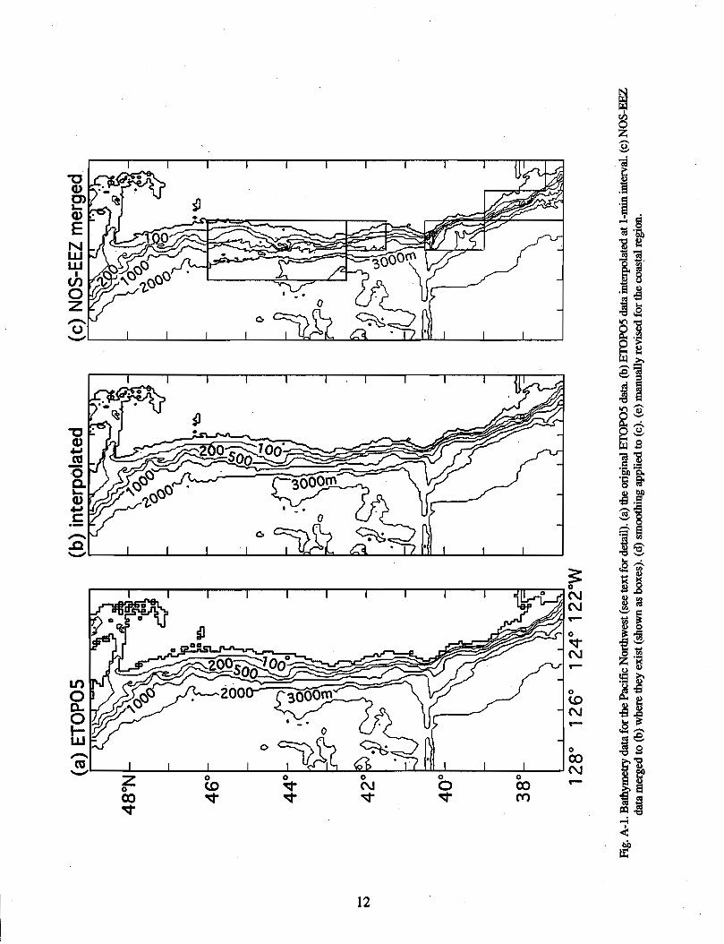
We started from ETOP05, a public domain bathymetry/topography data base with a grid size

of 5 min. Figure A-la shows the original ETOP05 data in our computation area. The ETOP05

bathymetry data are reasonably accurate in the deep (>500 m) ocean but are known to be inaccurate

in coastal water. Further, coastal shape cannot be accurately represented by 5-min grids. We first

interpolated the ETOP05 data to generate a I-min-grid bathymetry database (Fig. A-Ib). Obviously

the accuracy of these data is determined by that of the original ETOP05 data. For limited areas

within the U.S. Exclusive Economic Zone, gridded data with a lA-min interval are available from

National Ocean Service (NOS) on a CD-ROM. We averaged the lA-min data for each minute and

merged these to our interpolated data (Fig. A-Ie). The NOS-EEZ dat:a are compiled from multibeam

sounding data, and the coverage is shown in the boxed area in the figure. Within the boxed area, the

shallowest depth covered by the multibeam data is about 100 m. We then applied smoothing to the

merged data. As can be seen in Fig. A-Ie, the NOS-EEZdata show some irregularity. Tsunami

propagation is sensitive to the long wavelength bathymetry feature. Figure A4d shows the smoothed .

data. Finally, we manually updated the bathymetry data using NOAA bathymetry charts. The

manual editing was done from the coastline to the depth where the bathymetry charts and the

10

smoothed data are in reasonable agreement. This depth is about 100 m where we have NOS-EEZ data, but as deep as 1000 m where no NOS-EEZ data are available. The final bathymetry data we use for our computation are shown in Fig. A-Ie.

11

48°N

46

0

o

44

0

..­ N

380

12

80

12

60 1

240

122°

W

Fig

. A-I

. Bat

hym

etry

dat

a fo

r the

Pac

ific

Nor

thw

est (

see

text

for d

etai

l). (

a) th

e or

igin

al E

rOP

05

dat

a. (

b) E

rOP

05

dat

a in

terp

olat

ed a

t I-m

in in

terv

al. (

t:) N

OS

-EE

Z

data

mer

ged

to (

b) w

here

they

exi

st (s

how

n as

box

es).

(d)

sm

ooth

ing

appl

ied

to (

c).

(e)

man

uall

y re

vise

d fo

r th

e coas~

regi

on.

0

V N ~

0

to N ~

0.......... Q) CO

........... N .l'.§

~

~ '-' ...;

<I

oil t£:

'"C Q)

..c .f.J 0 0 E (J)

13

Appendix B: Inundation Model Description Charles L. Mader

Bl. Method of Inundation Modeling

Tsunami waves and their interaction with various topographies are numerically modeled using

the SWAN code. The SWAN code solves the incompressible, shallow-water, long-wave equations.

It is described in detail in the monograph Numerical Modeling o/Water Waves (Mader, 1988).

The incompressible, shallow-water, long-wave equations solved by the SWAN code are

aux au au aH u(lP. + u2Y> + u_x + u _x + g_ = FU + F(x) _ g x x yj (A5)

xat ax y ay ax C2(D + H-R)'Y

au· au au a'u u(lP. + U2r _Y + U-Y + U-Y + g_ll_ = -FU + F(Y)-g Y x y

at x ax Y x I )'ay ay C\D + H-R (A6)

and aH + a(D + H-R)Ux + a(D + Ji-R)Uy aR = 0 (A7) at ax ay at'

where U is velocity in x direction, Uy is velocity in y direction, g is gravitational acceleration, t isx

time, H is wave height above mean water level, R is bottom motion, F is Coriolis parameter, Cis

coefficient of DeChezy for bottom friction, p(x) and P(y) are forcing functions of wind stress in x and

y direction, and D is depth.

Flooding is described using positive values for depths below normal water level and negative

values for elevations above normal water level. Only positive values of the (D + H) terms in the

above equations were permitted. This method results in both flooding and receding surfaces being

described by the SWAN code.

The SWAN code has been used to study the interaction of tsunami waves with continental slopes

and shelves, as described in Mader (1975). Comparison with two-dimensional Navier-Stokes

calculations of the same problems showed similar results, except for short wavelength tsunamis.

The SWAN code was used to model the effects of tides on the Musi-Upang estuaries, South

Sumatra, Indonesia, by Hadi (1985). The computed tide and water discharge were in good agreement

with experimental data.

The SWAN code was used to model the large waves that were observed to occur inside Waianae

Harbor under high surf conditions (Mader and Lukas, 1985). These waves have broken moorings :r "

of boats and sent waves up the boat-loading ramps into the parking lot. The numerical mo~el was

able to reproduce act,ual wave measurements. The SWAN code was used to evaluate various.

proposals for decreasing the amplitude of the waves inside the Harbor. From the calculated results,

it was determined that a significant decrease of the waves inside the Harbor could be achieved by

decreasing the harbor entrance depth.

15

The effect of the shape of a Harbor cut through a reef on mitigating waves from the deep ocean

was studied using the SWAN code (Mader et ai., 1986). It was concluded that a significant amount

of the wave energy is dissipated over the reef regardless of the design of the Harbor. The reef

decreased the wave height by a factor of 3. The wave height at the shore can be further decreased

by another factor of 2 by a "V"-shaped or parabolic bottom design.

Other examples of applications of the SWAN code are presented in Mader and Lukas (1985).

They include the wave motion resulting from tsunami waves interacting with a circular and

triangular island surrounded by a 1/15 continental slope and from surface deformations in the ocean

surface near the island. The effects of a surface deformation in the Sea of Japan similar to that of

the May 1983 tsunami was modeled.

The SWAN code was used to model the effect of wind and tsunami waves on Maunalua Bay,

Oahu, as described by the State Department of Transportation (1988). The model reproduced the

observed wave behavior at various locations in the bay for a 1.2-m south swell with a 15-s period.

The code was used to model the interaction with Maunalua Bay of waves outside the Bay having

periods of 15,30, and 60 seconds and a tsunami wave with a 15-min period. Wave amplitudes of

0.3 to 1.8 m were considered with tides from mean lower low water to high tide (a 0.55-m range).

The 15-min period tsunami wave doubled in amplitude as it passed over the bay and was highest at

high tide. Severe flooding in the regions near the shore line was predicted. The calculated wave

behavior at any location in the Bay was a strong function of the entire Bay with a complicated and

time varying pattern of wave reflections and interactions.

The interaction of a tsunami wave with a site of well documented topography on the South

Kohala Coast of the Island of Hawaii was described by Mader (1990a). The tsunami wave was

calculated to flood the land to the 3-m level and inundate the land between 90 and 120 m from the

shoreline. These results agree with the results obtained using the procedures developed and applied

for flood insurance purposes by the U.S. Army Corps of Engineers and the recent study by JIMAR

at the University of Hawaii of tsunami evacuation zones for the region (Curtis and Smaalders, 1989).

The effect of tsunami wave period, amplitude, bottom slope angle, and friction on tsunami

shoaling and flooding has been investigated using the SWAN code, and a Navier-Stokes model was

reported by Mader (1990b).

The study shows higher wave shoaling and flooding for waves interacting with steeper slopes,

for waves with longer periods, and for waves from deeper water. The shallow-water waves shoal

higher, steeper, and faster than the Navier-Stokes waves. The differences increase as the periods

become shorter and slopes less steep with large difference for periods less than 500 s and slopes less

than 2 percent.

The interaction of the reflected first wave with the later waves often results in the second or third

runup being much different than the first runup. The magnitude and direction of the effect depends

upon both the slope and the wave period. For higher period waves, the second wave is as much as

a third larger than the first wave. The 1987-88 Alaskan Bight tsunamis were modeled by Gonzalez

16

et al. (1990) using the SWAN code. The deep-sea pressure gauge measurements for those tsunamis

could be described using realistic source models for the tsunamis.

An extensive numerical modeling study was performed by Mader and Curtis (l991a and b) of

the generation, propagation, and flooding of tsunami waves with Hilo, Hawaii. The flooding of Hilo,

Hawaii, by the tsunamis of April 1, 1946, May 23, 1960, and March 28, 1964, were numerically

modeled using the nonlinear shallow water code SWAN including the Coriolis and friction effects.

The modeling of each tsunami generation and propagation across the Pacific Ocean to the Hawaiian

Island chain was performed using a 20-min grid of ocean depths. This furnished a realistic input

direction and profile for the modeling of the tsunami interaction with the Hawaiian Islands on a

5-min grid. The resultant wave profile and direction arriving outside Hilo Bay was used to model

the tsunami wave interaction with the bay, harbor and town on a 100-m grid. Each element of the

grid was described by its height above or below sea level and by a DeChezy friction coefficient

determined from the nature of the topography.

The 1946 and 1964 tsunamis were generated by earthquakes in Alaska. The 7.5-magnitude 1946

tsunami flooding of Hilo was much greater than the 8A-magnitude 1964 tsunami. This was

reproduced by the numerical model. The directionality of the tsunami from its source was the

primary cause for the smaller earthquake resulting in greater flooding of Hilo. The 1960 tsunami was

generated by an earthquake in Chile. The observed largest wave was the third bore-like wave. The

numerical model reproduced this behavior. The observed levels of flooding" for each event was

reproduced by the numerical model with the largest differences occurring in the Reeds Bay area

where the local topography is poorly described bya 100-m grid. The observed levels of flooding at

individual locations were not well described by the 100-m grid, so a lO-m grid of Hilo was

developed to resolve the flooding at individual locations and around large buildings.

The high-resolution, lO-m grid of Hilo was used to model the flooding around Hilo Theater by

the 1960 tsunami wave. Hilo Theater was located near the shore. in flat and "unobstructed terrain

2.7 m above sea level. The tsunami flooded level reached 8.5 m at the seaward side and 6.7 m at the

rear of Hilo Theater. The third bore-like wave arriving at the harbor entrance in the 100-m grid

model was used as the tsunami source for the high-resolution study of flooding around Hilo Theater.

The maximum level of flooding observed at Hilo Theater was reproduced by the high-resolution

numerical model. The lO-m Hilo model now includes the major buildings in the city of Hilo and is

used to evaluate the effects of previous and potential tsunamis on the current topography, including

buildings.

The flooding of Crescent City, CalifoJllia, by the tsunami of March 28, 1964, has been

numerically modeled using the nonlinear shallow water code SWAN including the Coriolis and

friction effects. The results of the study are described in Appendix C (Mader and Bernard, 1993).

The modeling of the tsunami generation and propagation across the Pacific Ocean to the U.S. west

coast followed by modeling of the tsunami interaction with the west coast on a finer grid and then

17

modeling the tsunami wave interaction with Crescent City harbor and town using a high-resolution grid that reproduce the observed inundation limits.

The 1946 and 1964 tsunamis were.generated by earthquakes in Alaska. The 7.5-magnitude 1946 tsunami flooding of Hilo was much greater than the 8A-magnitude 1964 tsunami while the reverse was observed for Crescent City, California. This was reproduced by the numerical model. The directionality of the tsunami from its source was the primary cause for the smaller 1946 earthquake resulting in greater flooding of Hilo than the large 1964 earthquake. The directionality of the tsunami was also the primary cause for the extensive flooding of Crescent City by the 1964 event.

The tsunami wave generation, propagation, and runup modeling was performed using the SWAN code and the techniques that successfully reproduced the 1946, 1960, and 1964 tsunami inundation of Hilo, Hawaii, described by Mader and Curtis (l991a and b) and of Crescent City in Appendix C (Mader and Bernard, 1993).

B2. Inundation Model Bathymetry and Topography The numerical modeling of tsunami wave flooding requires detailed topographies of the region

of interest. The generation of the topography grids consists of first collecting all the data available for the area of interest, which are generally U.S. Geological Survey (USGS) topographic and NOAA bathymetry charts. The data are digitized using a Sumagraphic device. The grid resolution needed forthe numerical modelis chosen, and the SURFER software package generates the required grid from the digitized map data. The Krigging method was found to be the best SURFER option for preserving the important features of the digitized data. The details (e.g., coastal, river) that were lost in the Krigging process are edited by hand into the data files. The grids are tested in the SWAN code, and necessary corrections are again edited by hand into the data files. The topographic profiles for the Humboldt Bay and Eel River region, the Crescent City Bay and Harbor region, and the west coast are included in this appendix as contour plots and picture plots.

The Humboldt Bay and Eel River grid was generated using the USGS 7.5-min topo quads, 1:24,000, 1959, of Arcata North, Arcata South; Cannibal Island, Eureka, Fields Landing, Tyee City,

and the NOAA Nautical Bathymetry chart of Humboldt Bay, 1:25,000, 1983. The resolution of the grid was 100 m in the X and Y directions. The SURFER software package Krigging method was used for interpolation. The data represent the condition at approximately mean high tide.

The Crescent City grid was generated using the USGS topographic maps Crescent City, California, 1:24,000, 1966, and the Sister Rocks, California, 1:24,000, 1966 maps. The resolution of the grid was 25 m in the X and Y directions. The SURFER software package Krigging method was used for interpolation. The data files represent the high tide elevations and depths. The mean

range of the tide is approximately 2 m in the Crescent City region. The west coast from Humboldt County, California, to Flor~nce, Oregon, grid was generated

using the topographic maps ofWestern United States; Crescent City, 1:250,000, 1958, and Western United States; Eureka, 1:250,000, 1958, and the ETOPO data file 5-min grid.

18

Also used was Coos Bay, Oregon, 1:250,000, USGS 1958, Revised 1973; United States; Oregon­

Washington (Cape Blanco-Cape Flattery) 1:736,560, NOAA chart and the United States West Coast;

California-Oregon (Monterey Bay-Coos Bay) 1:811,980, NOAA chart.

The resolution of the grid was 1 kIn in the X and Y directions. The SURFER software package

Krigging method was used for interpolation. The data represent the condition at approximately mean

high tide.

B3. References

Curtis, G.D., and M. Smaalders (1989): A methodology for developing tsunami evacuation zones.

Proc. ofInternational Tsunami Symposium 89.

Gonzalez, F.I., C.L. Mader, M.C. Eble, and E.N. Bernard (1990): The 1987-88 Alaskan Bight

tsunamis: deep ocean data and model comparisons. Int. J. ofNatural Hazards, 4, 119-140..

Hadi, S. (1985): A numerical tidal model of Musi-Upang estuaries. A dissertation submitted to

Oceanography Department of University of Hawaii.

Mader, C.L. (1990a): Modeling tsunami flooding. Proc. ofPacific Congress on Marine Science and

Technology, PACON 90.

Mader, C.L. (1990b): Numerical tsunami flooding study-I. Science ofTsunami Hazards, 8, 79-96.

Mader, C.L. (1988): Numerical Modeling of Water Waves. University of California Press, Berkeley,

California.

Mader, c.L. (1975): Numerical simulation oftsunamis. J. Phys. Oceanogr., 5, 75-82.

Mader, C.L., and E.N. Bernard (1993): Modeling tsunami flooding of Crescent City. Proc. of

International Tsunami Symposium, TSUNAMI '93.

Mader, C.L., and G. Curtis (1991a): Modeling Hilo, Hawaii tsunami. Science ofTsunami Hazards,

91,85-94,

Mader, C.L., and G.D. Curtis (1991b): Numerical modeling oftsuna~ inundation ofHilo Harbor.

Joint Institute for Marine and Atmospheric Research contribution 91-251.

Mader, c.L., G.D. Curtis, and G. Nabeshima (1993): Modeling tsunami flooding of Hilo, Hawaii.

Proc. of Pacific Congress on Marine Science and Technology, PACON 92.

Mader, C.L., and S. Lukas (1985a): Numerical modeling of Waianae Harbor. Proc. 'Aha Huliko'a

Hawaiian Winter Workshop (January 1985).

Mader, C.L., and S. Lukas (1985b): SWAN-A shallow water, long wave code: Applications to

tsunami models. Joint Institute for Marine and Atmospheric Research report JIMAR 85-077.

Mader, C.L., M. Vitousek, and S. Lukas (1986): Numerical modeling of Atoll Reef Harbors. Proc.

International Symposium on Natural and Man-Made Hazards, Itimouski.

State Department of Transportation, Harbors Division (1988): Oahu Intraisland Ferry

System-Draft Environmental Impact Statement.

19

Appendix C: The JIMAR Tsunami Research Effort Engineering Model for Tsunami Inundation

George D. Curtis

Tsunami waves and their interaction with various topographies and the resultant inundation from known wave heights have been determined at JIMAR (Joint Institute for Marine and Atmospheric Research) for all of the coastlines in the State of Hawaii using the engineering technique described by Curtis and Smaalders (1989) and Curtis (l991a and b). The JIMAR Tsunami Research Effort (JTRE) engineering tsunami inundation and evacuation method was applied to Humboldt Bay, Eel River, and Crescent City. The method was developed for coastlines along the ocean. The method is less reliable or tested for enclosed bays such as Humboldt Bay and complex areas such as Crescent City Harbor.

The current set of tsunami evacuation maps for the State of Hawaii was generated at JTRE and. approved on January 31, 1991. The evacuation maps are published in the front of the telephone books for each of the islands and used by Civil Defense and local authorities.

The analytical method of Bretschneider and Wybro (1976) is used to estimate the inundation from waves with assumed constant heights and infinite periods at the shore line. Various cross

sectipns are taken of the topography from the shoreline and the limit of inundation for each cross section is determined. The friction along the cross section is described using Manning's friction

coefficient. The original formula was

2 2 113 2 h

2 = hl-~e + n g F h- ] [F + 1}1 Ax

~ (1.486)2 2 J

and had been rearranged for routine use as

(1.486)2

where h =wave height x =horizontal distance

hA =average depth F =Froude number

tan 8 =ground slope

Ax and Ah =incremental distance and height

n =Manning's friction coefficient

g =gravity

21

The runup height and inundation limit are calculated for each cross section and assumed wave

height at shoreline. The runup height is defined as the elevation of the ground above mean sea level

that the water will reach. This is usually not equal to the wave height, or inundation depth, at the

shore line. The inundation limit is the inland limit of wetting, measured horizontally from the mean

sea level line. The inundation limits are defined by connecting the limit points calculated for each

cross section along the appropriate topographic contours.

The JTRE model was applied to determine the tsunami inundation of Crescent City by a 10-,

5·, and 2-m wave and of the Humboldt Bay-Eel River area by'a 10- and a 2-m wave. Five cross

sections were modeled for Crescent City (see Fig. H-3). Cross sections perpendicular to the town

of Eureka, perpendicular to Fields Landing; and parallel to the Eel River were modeled for

Humbo~dt Bay and Eel River{see Fig. H-l). The friction was described using Manning's friction

coefficients, which were equivalent to the DeChezy friction coefficients used in the. numerical

models. The JTRE model and the numerical model gave similar inundation limits for Crescent City,

Humboldt Bay, and Eel River. This increases our confidence in our ability to model the inundation

limits and the reliability of our models for determining the inundation limits for the scenario

tsunami.

References

Bretschneider, C.L, and P.G. Wybro (1976): Tsunami inundation prediction. Proc. of 15th

Conference on Coastal Engineering, ASCE, Ch60.

Curtis, G.D. (1991a): Hawaii tsunami inundation evacuation map project. Joint Institute for Marine

and Atmospheric Research contribution 91-327.

Curtis, G.D. (l991b): Maximum expectable inundation from tsunami waves. Proc. ofInternational

Workshop on Long Wave Runup.

Curtis, G.D., and M. Smaalders (1989): A methodology for developing tsunami evacuation zones.

Proc. ofInternational Tsunami Symposium '89.

22�

Appendix D: Regional Model Verification Kenji Satake

Dl. Regional Model Calibration: The 1992 Petrolia Earthquake Tsunami To test the regional tsunami model described in Appendix A, we computed tsunamis from the

1992 Petrolia earthquake. We used fault parameters estimated from seismological and geodetic

analyses (Oppenheimer et aI., 1993). Figure D-l shows these parameters and the computed crustal

deformation, which predict the coast line uplift of 60 cm. This uplift was confirmed by field survey

(Oppenheimer et al., 1993).

We saved the computed tsunami waveforms at eight tide locations corresponding to existing

tide gauge stations. Figure D-2 shows comparisons of the observed and computed tsunami

waveforms (the tide has been removed from the observed records). One of the interesting features

of the observed tsunami waveforms is that they consist of two wave packets. This can be clearly

seen on the records at Crescent City, Point Reyes, or Monterey. More importantly, the maximum

height was registered by the second packet at more than a few hours after the first arrival of the

tsunami. The computed waveforms approximately reproduced these features. The amplitude and

waveforms do not exactly match at each station, but the overall agreement is quite good.

The numerical computation also shows the possible cause of the second packet. Figure D-3

shows the water height distribution at I-h intervals after the origin time of the earthquake. It is seen .

in the figures that the amplitudes are large along the coast for more than a few hours. At 1 h, the

largest peak (about 15 cm) is just outside the Eureka Bay entrance (40 0 40'). At 2 h, the largest peak

is at 41 o. If this movement of the peak represents a propagating wave, the apparent velocity is about

50 km/h. This corresponds to the velocity of a gravity wave for a depth of 20 m. Hence, this may

represent an edge wave, a kind of wave whose energy is trapped on the edge of the coast. The

observed late and large tsunamis are likely to be edge waves (Gonzalez etal., 1992).

D2. References Oppenheimer, D., G. Beroza, G. Carver, L. Denglar, J. Eaton, L. Gee, F. Gonzalez, A. Jayko, W.H.

Li, M. Lisowski, M. Magee, G. Marshall, M. Murray, R. McPherson, B. Romanowicz, K.

Satake, R. Simpson, P. Somerville, R. Stein, and D. Valentine (1993): The cape Mendocino

earthquake sequence of April 1992. Science, 261,433-438.

Gonzalez, F.I., E.N. Bernard, K. Satake, and Y. Tanioka (l992):'The Cape Mendocino tsunami,

25 April 1992 (abstract). Eos, Trans. AGU, Supplement, 505.

23

crustal deformation contour interval 20 cm 41 jJ

3()()() ~. --~

z ~'" ----\ -------'~'-,- ­

fault mode'···" \l\ -' - length: 21.5 km~ &~)

width: 16 knl ~.l ( .. depth: 6.03 krn (~~ 8 t

slip: 2.7 m ._- 0 0 I 39 ~ \\

126 125 124 123 longitude, W

Fig. 0-1. Crustal defonnation pattern computed from a fault model of the 1992 Petrolia earthquake by Oppenheimer et al. (1993). The solid and dashed contour lines show uplift and subsidence, respectively, with a 20-cm interval.

24

Po

rt

Orf

ord

10iii iii iii

iI

o

o

co

mp

ute

d

o

12

3 ~v

V5

0

12

34

5 ti

me

,ho

ur

D:.

50

E,SPi~

~

10

ri~

t ~e

yes

It

ob

serv

ed

o

bse

rve

d

O~A!\~~

.0

A

com

pu

ted

o1

23

45

o1

23

5 ti

me

,ho

ur

tim

e,h

ou

r

Fig.

0-2

. The

obs

erve

d (t

op)

and

com

pute

d (b

otto

m)

tsun

ami w

avef

orm

s at

eig

ht ti

de g

auge

sta

tion

s on

the

wes

t coa

st o

f the

Uni

ted

Sta

tes.

The

am

plit

ude

scal

es a

re

diff

eren

t for

eac

h st

atio

n bu

t the

sam

e fo

r th

e ob

serv

ed a

nd c

ompu

ted

wav

efor

ms.

The

tida

l com

pone

nts

wer

e re

mov

ed fr

om th

e ob

serv

ed w

avef

orm

s. T

ime

scal

e st

arts

at t

he o

rigi

n ti

me

of t

he e

arth

quak

e.

.

Fo

rt

Po

int

5 I

bi

I diii

I o

serv

e

o

iIi

I

o

co

mp

ute

d

co

mp

ute

d

o 5

o 5

tv

~

5 iii iii iii

o

i ,

Po

rt

San

L

uis

o 10

iii iii iii

i •

co

mp

ute

d

o 2

'3

tim

e,h

ou

r 5

o 1

2 3

. ti

me

,ho

ur

4 5

Fig

. D-2

. (co

ntin

ued)

.

Wat

er H

eigh

t D

istr

ibut

ion

2 hr

s 3

hrs

42oN

·L,

l--,~_

r-'-.-

---..-

-<::J~

~" ­

~

41°.

­

a

40

, 25

0W

12

4°

cont

our

inte

rval

: 5

cm

Fig

ure

D-3

. The

Com

pute

dw

ater

heig

htdi

stri

buti

ons ~t

eve

ry h

our a

fter t

he e

arth

quak

e al

ong

the

nort

hern

Cal

ifor

nia

coas

t. T

he so

lid ~d

das

hed

cont

our l

ines

indi

cate

po

siti

ve a

nd n

egat

ive

wat

er le

vels

, res

pect

ivel

y. w

ith

a 5-

cm in

terv

al.

Appendix E: Modeling of the April 1992 Eureka Tsunami Charles L. Mader

The tsunami of April 25, 1992, was caused by an earthquake centered south of Humboldt Bay

at Cape Mendocino with a magnitude of 6.9. The earthquake description used in the modeling was

developed by Frank Gonzalez of Pacific Marine Environmental Laboratory. The earthquake fault

parameters he used were 21.5-Ian long, 16-Ian wide, 6.3-Ian depth, 12-deg dip, 350-deg strike, and

94-deg rake. These parameters give the earthquake surface displacement shown in Fig. E-l. The axis

scale is 1 Ian.

A I-Ian grid along the Northern California coast was used to model the tsunami resulting from

the earthquake displacement. The I-Ian grid was 256 cells in the east-west direction and 221 cells

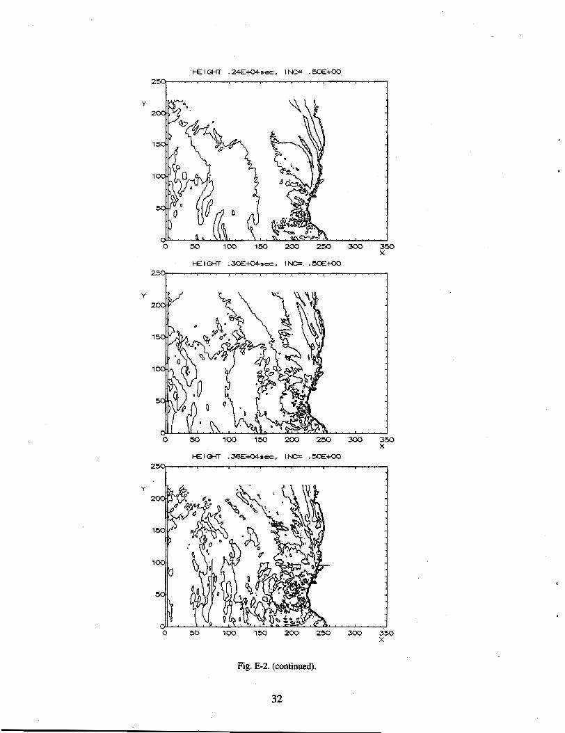
in the north-south direction for a total of 56,576 cells. The propagation of the tsunami from its

source is shown in Fig. E-2. Outside of Humboldt Bay, the tsunami wave had a complicated wave

train with a maximum height of 0.3 m. It was approximated as a sine wave with a height of 0.3 m,

a period of 1800 s, and an initially negative displacement. Outside of Crescent City, the tsunami

wave was a complicated wave train with a maximum height of 0.1 m and a period of 1,600 s. The

initial displacement was positive.

The interaction of a O.3-m-high, 1,800-s-periodtsunami wave outside of Humboldt Bay with

Humboldt Bay was modeled using a 100-m grid of Humboldt Bay (see Fig. H-l). The grid was

192 cells in the east-west direction and 255 cells in the north-south direction. The calculated wave

profile near the North Spit tide gauge and the smoothed gauge record are shown in Fig. E-3.

The interaction of a O.I-m-high, 1,600-s-period tsunami wave outside of Crescent City was

modeled using a 25-m grid (see Fig. H-3). The grid was 160 cells in the east-west direction and

240 cells in the north-south direction. The observed tide gauge record at Crescent City was higher

than the North Spit tide gauge and had a train of waves with a peak amplitude three times higher

than the maximum North Spit tide gauge amplitude and arrived 2 h after the first tsunami wave.

Only the arrival time of the first wave at Crescent City was reproduced by the numerical model. The

effects of tides were included in the calculations, but they did not significantly change the results.

29

1992 Eureka Quake Inc .4CE:+OO

r~ /

""------',_ I

(~,r[l] \,

o 10 20 30 40 50 50 70 X

1992 Eureka Quake Inc = .20E+OO

Fig. E-1. The April 25, 1992, Eureka earthquake surface displacement. The axis scale is 1 km.

30

I-EIGKT •20E+01 sec. INC= .5OE+OO

y

o 100 150 200 250 350 X

I-EIGKT • 12E+04sec•. INC= .5OE+OO

y

o

I-EIGKT .1SE+04sec. INC: .5OE+OO

25Or.......- .........---........"""'T""~---....,....~~ .........--~~ ...............---,

y

o 100 150 200 250 350 X

Figure E-2. The propagation of the April 25, 1992, Eureka tsunami from its source. Half-meter contour intervals are shown.

31

·I-EIGHT . 24E+04sec. INC= .5OE+OO

y

350 X

I-E I GHT • 3OE+04sec. I NC=. .5OE+OO

y

350 X

1-1:: I GHT •36E+04sec. INC= .5OE+OO

y

50 100 150 200 300 350 X

Fig. E-2. (continued).

32

Wove Height ot Locotion 7 0.6

__ NORTH SPIT H 0.4 TIDE GAUGE E I

G H 0.2 T

-0.0

-0.2

-0.4

-0.6 o 1000 2000 3000 4000 5000

Time

Figure E-3. The calculated wave profile near the North Spit tide gauge and the smoothed gauge record.

33

Appendix F: Verification of Crescent City Inundation Model

Reprint of Paper Appearing in Tsunami '93,

Proceedings of the IUGGIIOC International Tsunami Symposium

August 1993

35

TSUNAMI '93 Proceedings of the IUGG/IOC International Tsunami Symposium

International Tsunami Symposium of the Tsunami Commission of the International Union of Geodesy and Geophysics, and the International Coordination Group of the'lnternational Oceanographic Commission

Wakayama, ~apan

August 23-27, I 993

Organized by the •~apan Society of Civil Engineers

36

MODELING TSUNAMI FLOODING OF CRESCENT CITY

Charles L. Mader

Senior Fellow, JTRE - JIMAR 'l'sunami Research Effort University of Hawaii, Honolulu, HI., U.S.A.

E. N. Bernard

Director, Pacific Marine Environmental Laboratory

Seattle, WA., U.S.A.

ABSTRACT

The generation, propagation and interaction of tsunami waves with Crescent City, California is being numerically modeled for specific historical events. The modeling is performed using the SWAN code which solves the nonlinear long wave equations.

The March 28, 1964 tsunami was caused by an Alaskan earthquake. The tsunami generation and propagation across the Pacific was modeled using a 20 minute grid for the North Pacific. The wave arriving in the region of the U.S. west coast was modeled using a 5 minute grid. The wave arriving outside of Crescent City harbor was then modeled using a 25 meter grid of the harbor and town. The model gives approximately the observed maximum area of flooding of Crescent City. The large amount of flooding of Hilo, Hawaii from the 7.6 magnitude 1946 Alaskan earthquake and small amount offlooding from the 8.4 magnitude 1964 Alaskan earthquake at HHo while extensively flooding Crescent City was reproduced· by the numerical model. The effect of the tide was modeled and found to· be small.

37

MODELING

The flooding of Crescent City, California by the tsunami of 1964 was modeled using the SWAN non-linear shallow water code which includes Coriolis and frictional effects. The SWAN codeis deacribe4 in Reference 1. Most of tq.e calcul~tions were performed onan IBM PS/2 model 95~Hh16 megabyteaof memory. The 20 arid 5 minute topography

i.was obtained from the NOAA ETOPO 5 minute grid of the earth. The 25 meter grid \

topography was obtained using availabl~ USGS and other topographic maps, photographs and reports. The extent of flooding for the event is well documented.

The following calculations performed similar to the study of tsunami wave inundation of Hilo, Hawaii described in references references 2 and 3.

First - A 20 minute grid calculation of the North Pacific was performed to model the tsunami generation and propagation to the region of the West Coast of the United States. The 20 minute North Pacific grid was from 120 E to 110 W and 10 N to 65 Nand 390 by 165 cells. The wave profile arriving in the region of West Coast was used to select a realistic input direction and profile for the second step.

Second - A 5 minute grid calculation of the tsunami wave from the first step interacting with the West Coast was performed. The 5 minute West Coast grid was from 10 N to 60 Nand 240 by 480 cells. The wave direction and profile arriving in the region of Crescent City harbor was used to select a realistic input direction and profile for the third step.

Third - A 25 meter grid calculation of the tsunami wave from the second step interacting with Crescent City harbor and town, and the resulting flooding was performed using the input wave direction and profile from the second step. The 25 square meter Crescent City grid was 160 by 240 cells..

The results of the calculations were compared with the available Crescent City flooding levels for the 1964 tsunami.

The tsunami of March 28, 1964 was caused by an earthquake of 8.4 magnitude in Alaska near Prince William sound at 61 N, 147.5 W, 13:36 GMT.

The modeling of the tsunami wave formed by the earthquake and its interaction with Hilo, Hawaii was described in references 2 and 3. A summary of the results follows. The tsunami arrived at Hilo at about 17:30 HST. The second wave of the tsunami wave train was the largest. Using the first measurable half-wave period, the period was determined from the Hilo tide gage to be 50 minutes. The modeling of the tsunami wave formed by the earthquake and its interaction with Hilo, Hawaii was described in references 2 and 3. The earthquake source was studied in detail by Plafker (Ref. 5.). The source was 300 km wide and 800 km long aligned along a SW-NE direction. The source was 7 cells wide. The initial amplitudes from ocean to land had heights of +5.0, +9.0, +10.0, +9.0, +5.0, +1.0, -2.0 meters. This source resulted in a wave at Wake Island similar to that observed by Van Dorn (Ref. 4) as shown in references 2 and 3. The wave observed at Wake Island was 15 cm high with a 50 minute period.

The wave arriving north of the Hawaiian Islands was a half-wave with a period of 4000 sec, followed by a 0.1 meter high half-wave with a period of 2000 sec,then by a 0.25 meter high full wave with a period of 1750 sec.

The tsunami wave interacted with the Hawaiian Islands and refracted around the island of Hawaii such that the tsunami arrived from the North-East on the Hilo side ofthe island.

38

The wave arriving outside Hilo Bay had an initial positive amplitude of 1.0 meters, 4000 second period half-wave, followed by a 1.0 meter 2000 second period half wave, then by a 1.0 meter, 1750 period full wave. This wave was used as the source for the Hilo Bay calculation.

The calculated and observed inundation limits were much smaller than for the April 1, 1946 tsunami. Both the 1946 and 1964 tsunamis were generated by' earthquakes in Alaska. The 7.5 magnitude 1946 tsunami flooding of Hilo was much greater than the 8.4 magnitude 1964 tsunami. This was reproduced by the numerical model. The directionality of the tsunami from its source was the primary cause for the smaller earthquake resulting in greater flooding of Hilo. The 1946 tsunami wave peak energy was directed toward Hawaii while the 1964 tsunami wave peak energy was directed east of Hawaii toward the Pacific coast of North America as shown in Figure 1.

At the northern end of the West Coast of the United States the tsunami wave shown in Figure 1 has a period of 1500 seconds and a half-wave amplitude of about 2.0 meters shown as Location 7 in Figure 1. In the deep ocean the wave is coming from the North-West. It refracts as it travels down the coast and is coming from the West as it interacts with the region of Crescent city with height's of 4 meters as shown in Figure 2, Locations 6 and 7.

Figure 3 shows the calculated and observed inundation limit for Crescent City. The observed inundation limit was described in reference 6. The tsunami wave outside of the harbor had a height of 4.0 meters and a period of 1500 seconds. A constant DeChezy friction coefficient of 30 was used. The 1964 tsunami arrived just after high tide which contributed to the level of flooding. The tide was included in the model and the ebbing tide decreased the maximum water levels by less than 10 percent.

CONCLUSIONS

The flooding of Crescent City, California by the tsunami of March 28, 1964 has been numerically modeled using the non-linear shallow water code SWAN including the Coriolis and friction effects. The modeling of the tsunami generation and propagation across the Pacific Ocean to the U. S. West Coast followed by modeling of the tsunami interaction with the West Coast on a finer grid and then modeling the tsunami wave interaction with Crescent City harbor and town using a high resolution grid results in inundation limits that reproduce the observed inundation limits.

The 1946 and 1964 tsunamis were generated by earthquakes in Alaska. The 7.5 magnitude 1946 tsunami flooding of Hilo was much greater than the 8.4 magnitude 1964 tsunami while the reverse was observed for Crescent City, California. This was reproduced by the numerical model. The directionality of the tsunami from its source was the primary cause for the'smaller 1946 earthquake resulting in greater flooding of Hilo than the large 1964 earthquake. The directionality of the tsunami was also the primary cause for the extensive flooding of Crescent City by the 1964 event.

Acknowledgments

The authors gratefully acknowledge the contributions of George Curtis, Dr. Gus Furamoto, Dr. Harold Loomis, Dr. Lester Spielvogel, Dr. Doak Cox, Dr. Dennis Moore, Dr. Walter Dudley, Dr. George Carrier, Dr. Frank Gonzalez and the Pacific Tsunami Warning Center. George Nabeshima generated the 25 meter grids.

39

.6OE+02.ec. 1f'.C= .~+OO Wove Height at Location 2

H 2 E I

G H 1 T

/\ ­v v

-1

o 20 ..0 60 80 100 120 1..0 X

.7:£+04aec. INCa .~+OO

o 10000 1= y

Wove He 1g,t at Loeot Ion 7

H 2 E I G H 1 T

20 40 60 80 '00 120 140 X

.l4E+OealllC. INCa .~+OO -1

y -2

o 10000 20000 2eIOOO1= TIme

20 40 60 80 100 120 1..0 X

. leE+oe.aec. I NC= . 3e£+00 Figure 1. The March 28, 1964 tsunami wave movmg across the North Pacific Ocean. The contour interval is 0.35 meter. . Location 2 1S east of the island of Hawaii m 301 meters of water. Location 7 is west of Seattle, Washington in 2803 meters of water. and the tsunami wave for the West Coast calculation.

20 ..0 60 eo 100 120 1..0 X

40

. 1~+04.ec. INl> .70E+OO Way. He 1~t at Locat 1en ,

H E I .~ ~

....

2'CXO)l.....~.......,.l!>--~,O~--,."..l!> -~""20---=!2l!>· o 2000 4000 x

y

2'e<;O)l.....~.......,.l!>--~,O~-'-:,."..l!>-~""20:---'-~2l!> o 2000 4000 X

.6OE+04-."". 'NOW .701£+00 Wo". Heig,t ot Locat lon 7

y H

jE I G H ~

-. ....

2'CXO~---"l!>'-----:'::'O:---'-'-:'':-l!>-~~20::--~-:2l!> o 2000 4000 6000 X

. 7!)£+04sec. INC-. ?OE+OO

y

Figure 2. The March 28, 1964 tsunami wave interacting with the U. S. West coast. The contour interval is 0.70 meter. Location 1· is west of Seattle, Washington in .3660 meters of water. Location 6 is outside of Crescent City

2:CXOoJ--~""""'~---'-,O~--'''''~--""20--~.fl!> in 45 meters of w~ter and the tsunami wave for the Crecent City calculation. Location 7 is at the shore line of Crescent City.

.41

REFERENCES

1. Charles L. Mader Numerical Modeling of Water Wave8, University of California Press, Berkeley, California (1988).

2. Charles L. Mader and George D. Curtis "Numerical Modeling of Tsunami Inundation of Hilo Harbor" , JIMAR Contribution No. 91-251 (1991):

3. Charles L. Mader and George Curtis "Modeling Hilo, Hawaii Tsunami Inundation", Science of Tsunami Hazards, Vol 9, 85-94 (1991).

4. William G. Van Dorn, "Tsunami Response at Wake Island," Journal of Marine Research, Vol 28, no 3, 336-344 (1970).

5. G. Plafker, "Tectonics of the March 27, 1964 Alaska Earthquake," U. S. Geological Survey Professional Paper 543-1,11-174 (1969).

6. "The Great Alaska Earthquake of 1964," National Academy of Sciences (1972).

80 ~

,.---'" y ./

.... ~ 6

20

o 20 40 60 80 100 120 X

Figure 3. The calculated and observed inundation limits for Crescent City are shown for the tsunami of March 28, 1964. The observed limit is shown by a dashed line.

42

Appendix G: Earthquake Scenario Study with Regional Tsunami Model Kenji Satake

G1. Earthquakes

Testing the regional model by simulating the 1992 Petrolia earthquake/tsunami gave us the

confidence to model other earthquakes that might generate larger tsunamis. Using the regional

model, we generated four magnitude-8.4 earthquakes in the southern Cascadia Subduction Zone

(CSZ) and computed the propagation of the resultant tsunamis over a wide area of the U.S. west

coast. We .computed crustal deformation from realistic fault parameters and used it as an initial

condition for linear, long-wave propagation. The objectives of the regional computation were (1)

to model the generation and propagation of tsunamis on a regional scale and (2) to provide accurate

boundary conditions for local nonlinear inundation computations such as those presented in

Appendix B.

01.1. Seismological and Oeological Estimates ofFault Parameters

Figure G-1 defines the fault parameters. The vertical crustal deformation pattern can be

computed from these fault parameters using elastic dislocation theory (e.g., Okada, 1985,) .

01.1.1. Fault Length. The Cascadia Subduction Zone (CSZ) extends from the Mendocino

Fracture Zone on the south all the way to Queen Charlotte Fault, north of Vancouver Island (Fig.

G-2). The length ofthe entire CSZ is 1200 km. The length of the southern segment, south of Blanco

Fracture Zone, where Gorda plate is subducting beneath the North American plate, is 240 km. Thus,

earthquakes occurring within the southern segment of CSZ have.a maximum fault length of 240 km

(Clarke and Carver, 1992). If the rupture extends to the north, the fault may be longer, and the

earthquake may be as large as M=9. In southwestern Japan, a tectonically similar subduction zone

to CSZ (Heaton and Hartzell, 1987) exists where earthquakes with M=8 occurred periodically (Fig.

G-2).

01.1.2. Fault Width and Depth. Clarke and Carver (1992) hypothesized the fault width of the

Southern Cascadian event was 70 to 80 km. They assumed that the rupture extended seaward to the

western limit of strong coupling (seismic front or structural discontinuity), which is about 20 km

east of the CSZ (deformation front). The landward limit (aseismic front) is estimated to be where

the dip of the downgoing plate increases from -11 0 to 25 0 • This area also corresponds to the shallow

crustal seismicity. For tsunami generation, however, we also considered slips in shallower

extensions between the seismic front and CSZ. Studies of tsunamis in other places show that fault

slips generally extend all the way to the ocean bottom (e.g., 1946 Nankaidoearthquake or 1992

Nicaragua earthquake). The slip on the shallower part may be passive, or caused by the deeper slip,

but may affect the tsunami generation. We therefore considered two different fault widths: 80 km

and 100 km. The wider fault (100 km) extends to the ocean bottom at CSZ, while the narrower fault

43

latitude, longitude and depth North

'" ~,ete~ strike slip u

lengthL

Fig. 0-1. Fault parameters needed to compute crustal deformation pattern.

44

~ ... '"

"""

13

00 E

4A

3A J

. ~ -

... ••••••

• -" /".

~~~;:-

/

\.

7t'i )1·

7'.:?

"I J.

[\

.. .. .. 13

S0E

SOO

N

~

.. ..

'~l~

j!~

/)18~'b""'~

: o~~

......

......

..

: ~!;$fiA,~

2, '/

('

.. .. .. .. ..

4S0N

30

0 N

3S

0N

,

13

00 W

'!endo£..~Z.

, ,

, I

_ I

I I

,),

, !

.. , '4

0o N

1

20

0 W

Fig

. G-2

. Com

pari

son

oft

he C

asca

dia

Sub

duct

ion

Zon

e w

ith

the

sout

hwes

tern

Jap

an s

ubdu

ctio

n zo

ne w

here

M=

8 ea

rthq

uake

s oc

cur p

erio

dica

lly.

The

ori

gina

l fig

ure

is f

rom

Hea

ton

and

Har

tzel

l (19

87),

and

the

map

sca

les

are

appr

oxim

atel

y th

e sa

me.

extends only to the seismic front. Figure G-3.shows the cross sections of crustal deformation for

narrow and wide faults for the average slip of 8 m.

Gl.I.3. Fault Dip. The dip of seismicity is 10-200 in the northern CSZ (Crosson and Owen,

1987) and about 6 0 in the southern CSZ (Oppenheimer, personal communication, 1993). We

assumed that the dip angleis 100 and constant down to the aseismic front. Then the depth of the

seismic front or the upper edge of the narrower fault is about 5 km beneath sea level and the depth

of tlle aseismic front, or the deeper end of the fault, is about 20 km.

GI.IA. Average Slip on the Fault. The average slip is assumed to be 8 m on the main fault.

The convergence rate between the Gorda and North American plates is 30-40 mmlyr, and the

recurrence interval is 300 yr or longer (Heaton and Kanamori, 1984). There is no information on

what percentage of the slip is released seismically. One extreme is that the slip is aseismic; in this

case, there will be no large subduction earthquake. The other extreme is that the CSZ is completely

locked and there is no aseismic slip. Our estimate of 8 m is close to this case, assuming that an

earthquake of similar size occurred 300 years ago.

It is not critical that the slip estimate lJe exactly correct. As stated in Appendix A, tsunami

amplitude is linearly related to the average slip on the fault· as long as we use linear, long-wave

computation. Therefore, it is trivial to estimate tsunami amplitudes for different slip amounts.

GI.2. Slip Partitioning to Subsidiary Faults

Clarke and Carver (1992) put forward evidence of coseismic slip of the Little Salmon Fault

in Eureka Bay associated with the megathrust event. The Little Salmon Fault is part of a fault system

continuing out to sea in the accretionary prism. We therefore considered a case that the fault slip is

partitioned on these subsidiary faults.

Similar slip partitioning was observed for the 1964 Alaskan earthquake. The slip partitioning

onto a fault in shallow sediments has been proposed as a mechanism of a "tsunami" earthquake,

which produces tsunamis considerably larger than would be expected from seismic wave data

(Kanamori, 1972; Fukao, 1979).

Figure G-3 (bottom) shows the cross sections of crustal deformation for the slip partitioning

case. The 8-m slip is partitioned onto a subsidiary fault with a larger dip angle as well as onto the

extension of the main fault. The deformation pattern and amount is different from the above cases

and the tsunami excitation is expected to be different.

G13. Four Scenario Earthquakes.

We modeled four different scenario earthquakes. They are tabulated in Table G-l. Parameters

and computed crustal deformation are shown in Fig. G-4.

The model SW represents a rupture on wide (100 km) fault. The model SN represents a rupture

on a narrow (80 Ion) fault. The average slip· on these faults is 8 m. The seismic moments are

4.6 x 1028 dyne cm (1021 Nm) for the SN model and 5.8 x 1028 dyne cm (1021 Nm) for the

46

400

E Inarrow fault I u

+1' c cu E o Q) u ('lJ

C. .~ "'C

-400 -50 o 50 100 150

distance from CSZ, km

400

E Iwide fault I u

+1' c Q)

E Q)

0 CSZ

u ('lJ

c. (I)

.:0 o km

(OF)

I I

-400 -50 0 50 100 150

distance from CSZ, km

E400 I slip partitioned u

+1' c: Q)E

0

cu u ('lJ

a. (I)

:0

-400 -50 o 50 100 150

distance from CSZ, km

Fig. G-3. Cross section perpendicular to the fault strike (roughly east-west) showing the fault geometry and crustal deformation for three different models.

47

Table G~ 1. Fault parameters of four scenario earthquakes.

Fault Length

Case Main Subsidiary .Fault Width Top Depth Average Slip

SW(Wide 240km nla lOOkm Okm 8m SN (Narrow) 240km nla 80km 4km 8m SP 1 (Slip partitioning 1) 240km 235km lOOkm Okm 8m

(partitioned) SP 2 (Slip partitioning 2) 240km 85km l00km Okm 8m

(partitioned)

SW model, a~suming the rigidity is 3 x 1011 dyne/cm2• The moment magnitude, M ' for both cases w

is 8.4.

The models SP1 and SP2 represent the slip-partitioned cases. In model SP1, the slip is

partitioned onto the Little Salmon fault and its offshore extension, whereas in model SP2 the slip

partitioning occurs only on the Little Salmon fault. As can be seen in Fig. G-5 (c and d), the slip

partitioning gives very different crustal deformation in the Eureka area. The seismic moment is 5.2 x

1028 dyne cm for the SP1 model and 5.5 x 1028 dyne cm for the SP2 model. Both give M = 8.4.w

G2. Results of Regional Computations

G2.1. Eureka Area

The tsunami waveforms in the Eureka area from four earthquakes are shown in Fig. G-7 (see

Fig. G-6 for the locations). Among the four models, the tsunami amplitudes are largest from the case

SN at output points 1,2, and 3, while those from the models'SPl and SP2 become largest at output

points 4, 5, and 6. This local variation is due to the fact that the initial condition varies locally (see

Fig. 0-5). In fact, some of the largest amplitudes are associated with the crustal deformation; an

instantaneous uplift of the ocean bottom lifts the water mass above it. The predominant period of

tsunami is 50-60 min for all the cases, and the largest amplitude is 2.8 m (from SN) at 50-m depth.

At the North Spit tide gauge station, the maximum amplitude is 4 m from the model SN at about 3 h

after the earthquake. However, this amplitude is close to the water depth, and the nonlinear effect,

which was ignored in the computation, should become important to accurately evaluate the

amplitudes of such large tsunamis. Because this station is right above the Little Salmon Fault, the

coseismic deformation is larger than tsunamis for the models SP1 and SP2.

G2.2. Crescent City Area'

The tsunami waveforms in the Crescent City area are shown in Fig. 0-9 (see Fig. 0-8 for

locations). The tsunami waveforms from the four models are similar; three large waves arrive at

. about 15 min, 90 min, and 160 mins after the earthquake with similar amplitudes. The predominant

48

Case SW (Wide Fault) megathrust 'extends to the ocean bottom .

depth to the top edg.e= 0 km1w= lOa km

L = 150 km

strike N1OOW

dip 10°

400 58 1 N 124° 54 1W

slip 8 m L = 90 km (pure dip-slip) strike N200W dip 10°

40°1 1IN 124° 30'W r

depth to the top edge= 0 km

Fig. 0-4. Fault parameters for the four scenario earthquakes. See Figure 0-1 for the definitions of the parameters.

49

Case SN (Narrow Fault) . slip on seismogenic zone on megathrust

depth to the top edge= 4· km

1W==80km~.

L = 150 km

stri ke N1OOW

dip 10°

41 oN 124° 40'W

slip 8 m L = 90 km (pure dip-slip)

strike N200W· dip 10°

400 15'N 124°17'W

depth to the top edge= 4 km

Fig. 0-4. (continued).

50

Case SP1 case SN plus slip partitioning on Little Salmon Fault and its offshore extension

L: 1SO km .--t-t~

W: 30 km strike: N1OOW dip: 10° depth: 0 km slip: 4 m

L:90km W: 30 km strike: N20'W dip: 10° depth: 0 km slip: 4 m

L: 1SO km W: 70 km strike: N1OOW dip: 10° depth: 5 km

slip: 8 m

L: 1SO km W: 10 km strike: N100 W dip: 30° depth: 0 km slip: ·4 m

L =85 km W = 10 km strike NSOoW dip 20° depth 0 km slip 4 m

. 400 30.S'N 123° 54'W

L: 90 km W: 70 km

strike: N 200 W dip: 10° depth: 5 km

slip: 8 m

Fig. 0-4. (continued).

51

Case SP2 case SN plus slip partitioning only on Little Salmon Fault

L:90 km W: 30km strike: N200W dip: 10° depth: 0 km slip: 4 m

400 17'N 124°10'W

Fig. 0·4. (continlled).

52

L: 150 km W: 100 km strike: N1OOW dip: 10° depth: 0 km slip: 8 m

L =85 km W = 10 km strike NSOOW dip 200

depth 0 km slip 4 m

400 30.5'N 1230 54'W

L: 90 km W: 70 km

strike: N 200 W dip: 10° depth: 5 km slip: 8 m

Cas

e S

NC

ase

SW

43

1\

i

\(

II J

I )iii

iI 43

U'I

W

, --

... 1

'"

,•

I ,

'\ I

I '\

'\

; I :\ "

"

",

' ,

,",

' ,

,,'

" ,

,"

" ,

,.,

" ,

,II

" ,

,' ,

" ,

",

" ,

,' ,

" ,

,' ,

" ,

",

" ,

",

" ,

",

" ,

",

" ,

",

" ,

,n

" ,

" "

,~"

I,

" ,

", '

" ,

'11\

""

'I'

""

'",

""

,,,'

I "

, '\

\,"

" "

,\\

' "

,\\'

" ,

",

" ,

",

" ,

",

" ,

,\'

, , ,

\

\ \,

I ,

• \

\ J

I ,

\ \,

I,

\ '..

, /

\ I

'-'

41

42

<l>

'U

::J

-+oJ

-+oJ

o z

... -

.... ,

I ,

I _

....

'\

I'

'\

'\ I

" I

I ~"

,

,I

,"I"

, , ,'"

" ,

,"

" ,

,"

" ,

,"

" ,

,"

" ,

,"

" ,

, "

','

,",

" ,

",

" ,

",

" ,

I', II,

n,

",'

,

",

" ,

'" "

,,,

" , ,

'" "

,"'

''"'

",

'\t'

.' \\

' ,

H,' "',

"'\ "',

""

",

,"

"'it,

\\,

,\

, ,'

\\

It,

'" "

,'"

" ,

\\

'\ "

, \\

'\ "

, \\\

t ~

I '\

'\ "

• I

'\ '

\ ,

' ',

' , "

' "

41

42 z <l>

"'

0

::J

-+oJ

-+oJ

o

I

126

"'"

124

W

125 lo

ng

itu

de

.

'"

>,,

",

I I

, 4

0

123

I

126

\I'>

125 lo

ng

itu

de

.

I "I

'>

124

W

J1'

I I

, 4

0

123

Fig

. 0-5

. The

com

pute

d cr

usta

l def

orm

atio

n pa

tter

ns f

rom

the

give

n fa

ult p

aram

eter

s. T

he

soli

d an

d da

shed

con

tour

s in

dica

te th

e up

lift

and

sub

side

nce,

res

pect

ivel

y,

wit

h a

50-e

m in

terv

al.

Cas

e S

P1

Cas

e S

P2

43

'-',

,

"',-,

\

I,

\\

1\.

,;"

II'

, ,

III'"

,1\'

"

""

,,"

'",'II"

42

,II

".

I ,II

" ,

,'1

'1'

,II

I,

,

,II I,'z

," "

,,II

" ,

,'I

" ,

i"'"

.C

1)

~

I I

\ \\U

\1\\

\ \

1\\\\

\\ \

-g.II,

",

­""""

_ I,..

'.

"

, 0

',,,

," ,

',\\

I" ,

"\"

I,

,

, \\ .

..1 '"

41

\\\

",

,t\

" ,

,t\

" ,

,I'

" ,

,""1

""'1

,"'I

I'\

\.....

,1

\"

"

\'-'

"

' .....

.' -­

40

I \,

'\

I"'. '>

126

125

124

123

126

125

lon

git

ud

e.

W

lon

git

ud

e.

43

'-',

,I

-,

" \

" \

\I"

II"

,,

\1

",

,'I

",

I~

\"

, ,

'"

,I~",

--14

2 II,

" ,

,~,

'I

, ,

'"

,,~

",

"'I

,",

'I,

I Z

II ~

I'

, II

'"

,I'"

,

~

C1)

\\\

\\..

. -g

III

",

_,II"",

:;:i

II".

, "

, 0

""'"

,

,ll,

'"

,,\\,

I"

,

", ...

' '"

--I 4

1\\

\,"

, '\'

" ,

\\t

" ,

'""

,"""

"""

',"'1

',\1

1,

\\..

I ,

\'

...,' "

',_

.... '

"'

I I

, 4

0

124

123

W

Fig

. G-5

. (co

ntin

ued)

.

41°N J ~ \ c c ~

....... ~

40°50'

Fig. 0-6. The grid system used for the regional modeling around the Eureka area. The computed waveforms are output at six points on the 50-m depth and the North Spit tide gauge location, as shown by solid squares.

55

(a)�

(b

)

off

E

urek

a 1�

o

ff

Eu

reka

2

em

em

20

0

ma

x:

20

0�

ma

x:

282.

� 22

6.

SN

0�

S

N

0m

in:�

m

in:

-21

9.�

...

.;206

.

20

0

ma

x:

20

0�

ma

x: .

22

8.�

196.

SW

0�

SW

0m

in:�

m

in:

-19

8.�

-1

85

.

(.It

0

'\

20

0�

ma

x:

20

0

ma

x:

21

3.�

20

4.S

P1

0�

SP

1 0

min

:�

min

: -2

18

.�

-:22

2.

20

0

ma

x:

20

0�

ma

x:

21

7.�

20

3.S

P2

0�

SP

2 0

min

:�

min

:·

"'2

16

.�

-20

8.

1"",1

"",1

"",1

"",1

�I"", I

"", I

"", I

"", I

o�

1

23

4

o 1

23

4

tim

e,.

ho

ur

tim

e,

ho

ur

Fig

. 0-7

. The

com

pute

d ts

unam

i wav

efor

ms

from

the

four

mod

els

at s

ix o

utpu

t poi

nts

at 5

0-m

dep

th (

a-t)

and

at N

orth

Spi

t tid

e ga

uge

stat

ion

(g).

(c)

(d)

em

200

SN

0

off

E

ure

ka

3 m

ax:

223.

m

in:

-25

1.

em

200

SN

0

off

E

ure

ka

4 m

ax:

224.

m

in:

-21

9.

200

SW

0

max

: 18

5.

min

: -1

80

.

200

SW

0

max

: 15

6.

min

: -1

95

. V

I-:a

20

0

SP

l 0

max

: 2

16

. m

in:

-21

2.

200

SP

l 0

max

: 25

9.

min

: -1

82

.

200

SP

2 0

max

:' 207.

m

in:

-19

9.

200

SP

2 0

max

: ·2

55

. m

in:

-17

9.

1"",1

"'1

11

"",1

"",1

o 1

23

4

tim

e,

ho

ur

1"",1

"",1

"",1

"",1

o 1

23

4

tim

e,

ho

ur

Fig

. G-7

. (co

ntin

ued)

.

(e)

SN

em

20

0

0

off

E

ure

ka

5

20

0

SW

0

Vl

00

2

00

SPl

0

20

0

SP2

0

1 I

o I

I I

I 1

I

1 I

I I

I 1

I I II

I 1

I I

I I

I 1

23

4

tim

e.

ho

ur

max

: 23

2.

min

: -2

32

.

max

: 14

5.

min

: -1

92

.

max

: 27

0.

min

: -1

72

.

max

: 27

7.

min

: -1

69

.

SN

SW

(f) . o

ff

Eu

reka

6

em

20

0

0

20

0

0

200

SP

l 0

20

0

SP2

0

11

11

11

I1

11

11

11

11

11

11

11

11

1

o�

1 2

34

ti

me

. h

ou

r

max

: 23

1.

min

: -2

24

.

max

: 14

4.

min

:. -1

93

.

max

: 24

9.

min

: -1

75

.

max

: 25

7.

min

: -1

69

.

Fig

. G-7

. (co

ntin

ued)

.

(9)

SN

em

500 0

No

rth

S

pit

m

ax:

400.

m

in:

-29

7.

500

SW

0

max

: 35

8.

min

: -2

46

.

VI

\.0

50

0

SP

1 0

max

: 26

5.

min

: -2

94

.

500

SP

2 m

ax:

244.

m

in:

-27

0.

o 1

2 3

tim

e.

ho

ur

1"",1

"",1

"",1

"",1 4

Fig

. G-7

. (co

ntin

ued)

.

41 °50'

N o o "3

Fig. G~8. The grid system used for the regional modeling around the Crescent City area. The computed waveforms are output at six points on the 50-m depth and the Crescent City tide gauge location. as shown by solid squares.

60�

(a)

(b)

em

off

C

resc

en

t C

ity

1 em

o

ff

Cre

sce

nt

City

2

20

0

max

: 2

00

m

ax:

SN

26

2.

min

: S

N

221.

m

in:

-24

0.

-26

5.

max

: 2

00

m

ax:

158.

m

in:

SW

0 18

2.

min

: -1

88

. -1

93

.

0\ -

max

: m

ax:

218.

21

2.

min

: m

in:

-20

7.

-23

6.

max

: m

ax:

159.

m

in:

SP2

204.

m

in:

-18

7.

-19

1.

'1

11

11

'1

11

11

'1

11

11

'1

11

11

'

'1

11

11

11

11

11

'1

11

11

11

11

11

'

o 1

23

4

o 1

23

4

tim

e•.

ho

ur

tim

e.

ho

ur

Fig

. G-9

. The

com

pute

dts

unam

i w

avef

orm

s fr

om t

he f

our

mod

els

at s

ix o

utpu

t poi

nts

(a-f

) an

d C

resc

ent C

ity

tide

gau

ge s

tati

on (g

).

(c)

(d)

off

C

resc

en

t C

ity

3 e

m

. e

m

off

C

resc

e,n

tCit

y 4

SN

20

0 0

ma

x:

250.

m

in:

-26

9.

SN

20

0 o

ma

x:

242.

m

in:

-23

6.

20

0

SW

0

ma

x:

21

8.

min

: -2

07

. o

20

0

SW

ma

x:

232.

m

in:

-19

6..

~

20

0

SP

1 0

ma

x:

,,258

. m

in:

-23

3..

20

0

SP

1 0

ma

x:

245.

m

in:

-22

2.

20

0

ma

x:

20

0

ma

x:

SP

2 0

235.

m

in:

SP

2 0

231.

m

in:

-21

1.

-20

3.

1"",1

"'1

,1"",1

"",1

o 1

23

4

1"'1

,1"'1

11

"",1

"",1

o 1

23

4

tim

e,

ho

ur

tim

e,

ho

ur

Fig

. G-9

. (co

ntin

ued)

.

(e)

(f)

off

C

resc

en

t C

ity

5 em

o

ff

Cre

sce

nt

City

6

em

SN 20

0 0

ma

x:

244.

m

in:

-23

2.

SN 20

0 0

ma

x:

250.

m

in:

-28

3.

200

SW

0

ma

x:

240.

m

in:

-19

1.

200

SW

0

ma

x:

253.

m

in:

-21

7.

0\

w

200

SP

1 0

ma

x:

257.

m

in:

-21

6.

200

SP

1 0

ma

x:

258.

m

in:

-23

3.

200

ma

x:

200

ma

x:

SP

2 0

244.

m

in:

SP

2 0

256.

m

in:

-22

0.

-21

3.

1 ••••• 1

••••• 1

••••• 1

••••• 1

1 ••••• 1

••••• 1

••••• 1

••••• 1

o

1 2

34

o

1 2

34

ti

me

, h

ou

r ti

me

, h

ou

r

Fig.

0-9

. (co

ntin

ued)

.

(9) .C

resc

en

t C

ity

em

50

0

ma

x:

567.

S

N

0 m

in:

-46

4.

50

0

ma

x:

46

3.

SW

0 m

in:

-43

7.

~

50

0

ma

x:

573.

SP

1 0

min

: -4

41

.

50

0

ma

x:

536.

SP

2

0 m

in:

-42

1.

I!

!.!

! !

II

!!

I!

II

!!

I!

I!

! !

!!

I o

1 2

34

ti

me

, h

ou

r

Fig.

0-9

. (co

ntin

ued)

.

period of 60-80 min and the amplitude is about 2.5 m at 50-m depth. At the Crescent City tide gauge

location, the maximum tsunami height is about 5 m from all the models, and it occurs about 160 min

after the earthquake. Again, the estimates of tsunami heights at tide gauge station is not very

accurate, because of the nonlinearity. Further, our computation for the 1992 Petrolia earthquake

(Fig. D-2) underestimated the tsunami height at this tide gauge station.

G3. Conclusion The regional tsunami modeling was made for four M -8.4 earthquakes and tsunami waveforms w

are computed at 50-m depth offshore Eureka and Crescent City. The worst-case

tsunami has an amplitude of 2.9 m and a period of 5Q-60 min offshore Eureka, 2.5-m amplitude, and

60-80-min period offshore Crescent City. These provide realistic boundary conditions for mode­

detailed inundation modeling for both areas.

G4. References Clarke, S.H., and G.A. Carver (1992): Late Holocene tectonics and paleoseismicity, southern

Cascadia Subduction Zone. Science, 255, 188-192.

Crosson, RS., and TJ. Owen (1987): Slab geometry of the Cascadia Subduction Zone beneath

Washington from earthquake hypocenters and teleseismic converted waves. Geophys. Res.

Lett., 14, 824-827.

Fukao, Y. (1979): Tsunami earthquakes and subduction processes near deep-sea trenches.

J. Geophys. Res., 84,2303-2314.

Heaton, T.H., and S.H. Hartzell (1987): Earthquake hazards on the Cascadia Subduction Zone.

Science, 236, 162-168.

Heaton, T.H., and H. Kanamori (1984): Seismic potential associated with subduction in the

northwestern United States. Bull. Seism. Soc. Am., 74,933-941.

Kanamori, H. (1972): Mechanism oftsunami earthquakes. Phys. Earth Planet. Inter., 6,246-259.

Okada, Y. (1985): Surface deformation due to shear and tensile faults in a half-space, Bull. Seism.

Soc. Am., 75, 1135-1154.

Oppenheimer, D., G. Beroza, G. Carver, L. Denglar, J. Eaton, L. Gee, F. Gonzalez, A. Jayko, W.H.

Li,M. Lisowski, M. Magee, G. Marshall, M. Murray, RMcPherson, B. Romanowicz, K.

Satake, R Simpson, P. Somerville, R Stein, and D. Valentine (1993): The Cape Mendocino

earthquake sequence of April 1992. Science, 261,433-438.

65�

Appendix H: Tsunami Inundation� Charles L. Mader and George Curtis�

HI. Eureka The interaction of a tsunami wave similar in maximum amplitude to the April 1992 Eureka

tsunami and a lO-m incident tsunami with Humboldt Bay and Eel River was modeled. The

topographic grid was 100 m square, and the friction was described with a DeChezy coefficient. The

areas normally under water had a coefficient of 40, while most of the land areas had a coefficient

. of 30. Populated areas with buildings had a coefficient of 10 as did regions with heavy timber. The

model had 192 cells in the east-west direction and 375 cells in the north-south direction for a total

of72,000 cells. The calculations were performed on 50-MHz, 486 personal computers using the

OS/2 operating system and the SWAN computer code with MCGRAPH graphics.

The tsunami wave similar to the April 1992 event was described by a2-m-high tsunami wave

in 50 m of water with a period of 33.3 min. The southern end of the Humboldt spit was flooded. The

Eel River region was flooded inland as much as 2.5 km. Only the region across from the Bay

entrance was flooded inside the Bay.

The Cascadia Subduction Zone earthquake was modeled using a lO-m-high tsunami wave in

50 m of water with a 33.3-min period. All the Humboldt spit was flooded. The inundation levels

inside the harbor reached 3 m at some locations and extended inland over 5.0 km in the Eel River

region.

The inundation area for the lO-m tsunami is shown in Fig. H-1 with the X and Y axis being

the grid number or 100 m. The lines labeled A, B, and C are the one-dimensional engineering model

locations used to cross check the inundation model. Favorable comparisons led to the conclusion

that the inundation model was performing properly.

H2. Crescent City The interaction of a tsunami wave similar to the April 1964 event and a lO-m incident tsunami

with Crescent City harbor and town was modeled. The topographic grid was 25-m square, and the

friction was described with a DeChezy coefficient of 30, which is appropriate for most of the

flooded area. The model had 160 cells in the east-west direction and 240 cells in the north-south

direction for a total of 38,400 cells. The calculations were performed on 50-MHz, 486 personal

computers using the OS/2 operating system and the SWAN computer code with MCGRAPH

graphics.

The tsunami wave similar to the April 1964 event was described by a 5-m-high tsunami wave

in 50 m of water with a period of 33.3 min. All the land below 2-m elevation was flooded, and the

inundation levels inside the harbor reached 4 m at some locations and extended inland over 600·m.

The Cascadia Subduction Zone earthquake was described by a lO-m-high tsunami wave in

50 m of water with a 33.3...min period. All the land below 4 m elevation was flooded and the

67�

Humboldt Bay� Tsunami Inundation Limits�

400

350 ­

300 ­

250 - A -------'

200 ­

B ----~"----__'8!I.

150 ­

100 ­

50 ­

c�

o� o 100 200 300

100 Meter Increments

Fig. H- I. The Humboldt Bay and the Eel River region inundation areas for a IO-m, 33.3-min-period high tsunami. Lines labeled A, B, and C represent the locations of the engineering model used to cross check the inundation model calculations. The length of the line represents the extent of flooding estimated by the engineering model.

68�

inundation levels inside the harbor reached 6 m at some locations and extended inland over 1.3 lan.

The wave heights as a function of time at seven locations are shown in Fig. H-2. The locations are

shown as dots with their location numbers. The depths at the various locations are, in order, 22.6 m,

7.9 m, and 6.4 m below high tide and 3.1 m, 0.2 m, 3.0 m, and 2.7 m above high tide. The maximum

water level over land was 8 m for locations 4, 5, and 6.

The inundation area for the lO-m tsunami is shown in Fig. H-3 with the X and Y axis being

the grid number or 25.0 m. The lines labeled A through E correspond to the locations of the one­

dimensional engineering model used to cross check the inundation model performance.

69�

y . 1 LOCATIONS

o 100 1&l 200

Wave I-Ie i g,t at Locot ion 1

-1"'-~~"""'--~"""'--~"""'-----"""-----:':' o &>0 1000 1&>0 2000 2&>0 Time

Wave I-Ie i g,t at Locot ion 2

H� E� I�

G� H� T�

_1Q1-_~_--'----,.__""""' ..........J"""" """'__.....-J�

o 1000 1&>0 2000 2&>0 Time

Fig. B-2. The wave heights as a function of time at various Crescent City locations for a 10-m-high tsunami wave in 50 m of water with a 33.3-min period. .

70�

WQve He i Q-tt Qt LoQQt i en 4

H e: I

G H .T

1000 2000 2eoo Time

H e: I

G H T

. _ 101-...... ""­__~-10 ......__.J.-_~_--l. --'

o 1000 1&>0 2000 2&>0 Time

Fig. H·2. (continlied)~

71

Wove Hei 9"'t ot I.QCCIt ion .6

H� E� I�

G H T

-1cJ­ -'­ -'­ -'-_......_-'-_................J

o ~ 1000 11JOOZXlO ~ Time

Wove He i 9"'t ot l.=t ion 7

H E I

G H T

-1o-_........_ ...... ...... ..... ...... ..J�

o� . 1000 ,:.00 2000 2:$00 Time

72�

Crescent City� Tsunami Inundation Limits�

250 ~-----------------------------,

A

200

150

100

N

~

50

o o 50 100 150

25 Meter Increments

Fig. H-3. The Crescent City inundation areas for a lO-m, 33.3-min-period high tsunami. Lines labeled A, B, C, D, and E represent the locations of the engineering model used to cross check the inundation model calculations. The length of the line represents the extent of flooding estimated by the engineering model.

73

Appendix I: Cascadia Subduction Zone Earthquake Scenario Meeting

Attendees at Cascadia Subduction Zone Scenario Earthquake Meeting

Held April 8, 1993, at California Division of Mjnes and Geology, Sacramento, California

U.S. Geological Survey� David Oppenheimer� Samuel H. Clarke�

Federal Emergency Management Agency� Jim Buika-Region 9� Christine Jonientz-Trisler-Region 10�

National Oceanic and Atmospheric Administration� Eddie Bernard-.Pacific Marine Environmental Laboratory�

California Division of Mines and Geology� James Davis� Tousson Toppozada� Michael Reichle� Glenn Bornhardt�

California Office of Emergency Services� Ed Bortugno� Paula Schulz�

California Seismjc Safety Commission� Richard McCarthy�

University of California at Berkeley� Robert Olson�

Humboldt State University� Gary Carver�

University of ,Michigan� Kenji Satake�

Woodward-Clyde Consultants� Ivan Wong�

·75

STATE OF CALIFORNIA-THE RESOURCES AGENCY PETE WILSON, Governor

DEPARTMENT OF CONSERVATION

DIVISION OF MINES AND GEOLOGY GEOLOGIC HAZARDS ASSESSMENT PROGRAM 801 K STREET, MS 12-31 SACRAMENTO, CA 95814·3531 Phone (916) 324·7299

April 23, 1993

Dr. E. Bernard� Pacific Marine Env. lab.� 7600 San Point Way NE Bldg. 3� Seattle, WA 981150-0700�

Dear Colleague:

This is a follow-up to the meeting of 8 April regarding the scenario earthquake on the Cascadia subduction zone (CSZ) in northern California. The fault parameters agreed upon were as follows:

length 240 km� Width 80-100 km� M 8% Displacement 8 m Dip of CSZ 10° Western extent of rupture on CSZ - 20 km E of CSZ trace Depth of western limit of CSZ seismic rupture 6 - 7 km (water depth is 0.5 to 1 km) Southern extent of CSZ near April 1992 epicenter Duration - 1 minute (>0.05g and >2Hz).

The attached map shows the geometry of the fault planes. The coordinates of the points are listed, so that different modelers can use the same geometry. The points are listed in order, clockwise from Petrolia (P).

. -­RECEIVED APR 2 J 1993

76 PMEL

-2­April 23, 1993

P 40°20' 124°17' AB�

41 °0' 124°40'� 41 ° 17' 124°49'�

C 41 °52' 125°0'� oE�

42°19' 125°0'� 42°19' 123°40'�

F 40°36.5' 123°40' G 40°30.5' 123°54' H 40°32.5' 124°0' I 40°35.6' 124°7' J� 40°38.6' 124°10.3'� K 40°41.3' 124°11.6'�

The area (PABCDEF) is about 19,000 km2 , leading to Mw 8.4 using Wyss (1979).

Gary Carver suggested that the 8 m displacement on the CSZ be partitioned, with 4 m going to the Little Salmon fault (LSF), which dips about 20°. In that case, .. d = 8 m on CSZ between points 0 and A, and d =4 m between A and P, and d =4 on LSF between A and G. We are not yet sure how to model the shaking intensities from a combined CSZ-LSF event.

I would appreciate any comments you may have on the fault parameters or geometr·y. Thank you very much for your cooperation.

Sincerely,

~~ T.~a~ Senior Seismologist

TRT:vw

attachment

77�

State of California The Resource Agency

Memorandum

To: Kenji Satake. Mark Murray. David Oppenheimer Date: May 4. 1993

From: Tousson R. Toppozada Department of Conservation Division of Mines and Geology

~??/ ~..-r[ ./. 1 801 K Street. MS 12-31 Sacramento 95814-3531

Subject: Cascadia Fault Parameters

I have received e-mail from David and Kenji at CDMG @andreas.wr.usgs.gov, regarding my

letter and map of April 23rd. I will address my comments to the question numbers used by

them.

1. What is the geometry of the Little Salmon Fault? Kenji has answered David's question.

3. Could the fault be treated as a rectangular fault instead of the wavy line shown in the

map? I thought David was still referring to LSF. But Kenji is referring to CSZ.

Kenji, it is ok to ignore line EF, and to measure 80 km east of points D, C, B, A, and P, to

have a uniform width of the seismogenic segment of the CSZ.

4. What is the boundary between 4 and 8 meter slip region of the CSZ? Point A to where?

(keep latitude of 41 degrees?) David's question of where the EW boundarioes intersect line EF

is addressed in the previous paragraph.

In addition to the two cases mentioned by Kenji, there is a third case that Sam Clarke

and Gary Carver indicate was discussed in the April 8 meeting:

4 m on AP, 4 m on AG, which is the same as Kenji's case (2) south of A. Then north

78�

from A, 4 m on ABCD, and 4 m on A'B'C'D', where A' is on CSZ map trace, 20 km W of

A, and so on for B'C' and 0 ' . This third case is the only one that has surface rupture 14m)

branching up on a steep splay to the ocean bottom at the western edge of the seisomgenic

zone at ABeD. Cases 1 and 2 have the 8m rupture propagating from ABCD aseismically tJp­

dip at .... 10° to the ocean bottom surface at A/B/C/D/.

This third possible case has no effect on the intensities on land.

5. What is the strike of the "two" CSZ faults and the rake of all "three" faults? Kenji

addresses this question adequately. I would like to note that BP is a straight line, so that

the strikes of BA and AP are equal. A is just the projected intersection of LSF with BP.

A pure dip-slip "rake of 90 0 is reasonable. Clarke also noted the length of 230 km for

DCBAP, and indicated that it could be extended to 240 km by moving point P some 10 km

due S (or 10 km ESE along BAP).

6. What is the elevation datum for the region of interest (Le., the seafloor)? Is a single flat

surface layer sufficient? I have no comment on the datum.

cc:� Eddie Bernard

Gary Carver

Sam Clarke

Ivan Wong

79�

o

I\i--\\ ·.-----.....-----r--r Iff'

. I

t, z" --~---"..... -44;:·,,,-,

~ Anllcllne

f Syncline

J-.A.. Th,,,sl faull . . barbs on upper pia I Q

...

80 * u.s. GOVERNMENT PRINTING OFFICE 673-886